Topics in Shear Flow Front Matter Donald Coles �

Professor of Aeronautics, Emeritus

California Institute of Technology Pasadena, California

Assembled and Edited by

�Kenneth S. Coles and Betsy Coles

Copyright 2017 by the heirs of Donald Coles

Except for figures noted as published elsewhere, this work is licensed under a Creative Commons Attribution-NonCommercial-ShareAlike 4.0 International License

DOI: 10.7907/Z90P0X7D

The current maintainers of this work are Kenneth S. Coles (kcoles@iup.edu) and Betsy Coles (betsycoles@gmail.com)

Version 1.0 December 2017

Topics in Shear Flow

Version 1.0

Topics in Shear Flow

Donald ColesProfessor of Aeronautics, EmeritusCalifornia Institute of Technology

Pasadena, California

Assembled and Editedby Kenneth S. Coles and Betsy Coles

December 2017

c©Copyright 2017 by the heirs of Donald Coles

Except for figures noted as published elsewhere, this work islicensed under a Creative Commons

Attribution-NonCommercial-ShareAlike 4.0 International License

DOI: 10.7907/Z90P0X7D

The current maintainers of this work are Kenneth S. Coles(kcoles@iup.edu) and Betsy Coles (betsycoles@gmail.com)

Version 1.0 December 2017

Suggested citation: Coles, Donald (2017). Topics in Shear Flow.DOI: 10.7907/Z90P0X7D

Contents

Preface xxv

1 INTRODUCTION 1

1.1 Generalities . . . . . . . . . . . . . . . . . . . . . . . . 1

1.2 Analytical prologue . . . . . . . . . . . . . . . . . . . . 5

1.2.1 Definitions and identities . . . . . . . . . . . . 5

1.2.2 Equations of motion . . . . . . . . . . . . . . . 7

1.2.3 Incompressible fluids . . . . . . . . . . . . . . 15

1.2.4 Low-speed heat transfer . . . . . . . . . . . . . 21

1.2.5 The Boussinesq approximation . . . . . . . . . 25

1.2.6 Coordinate systems . . . . . . . . . . . . . . . 29

1.3 Operational prologue . . . . . . . . . . . . . . . . . . . 29

1.3.1 Stream functions . . . . . . . . . . . . . . . . . 29

1.3.2 Boundary-layer approximations . . . . . . . . 30

1.3.3 Subcharacteristics . . . . . . . . . . . . . . . . 40

1.3.4 Reynolds averaging . . . . . . . . . . . . . . . 44

1.3.5 Dimensions and similarity . . . . . . . . . . . 48

2 PIPE FLOW 59

i

ii CONTENTS

2.1 Generalities . . . . . . . . . . . . . . . . . . . . . . . . 59

2.1.1 Equations of motion . . . . . . . . . . . . . . . 60

2.1.2 Laminar flow . . . . . . . . . . . . . . . . . . . 64

2.1.3 An extremum principle . . . . . . . . . . . . . 68

2.2 Development length . . . . . . . . . . . . . . . . . . . 71

2.2.1 Laminar flow . . . . . . . . . . . . . . . . . . . 71

2.2.2 Capillary-tube viscometry . . . . . . . . . . . 76

2.2.3 Turbulent flow . . . . . . . . . . . . . . . . . . 98

2.3 Transition . . . . . . . . . . . . . . . . . . . . . . . . . 103

2.3.1 Intermittency . . . . . . . . . . . . . . . . . . 103

2.3.2 Methods of measurement . . . . . . . . . . . . 109

2.3.3 The puff and the plug . . . . . . . . . . . . . . 114

2.3.4 Short account of flow in coiled pipes . . . . . . 120

2.3.5 Splitting . . . . . . . . . . . . . . . . . . . . . 121

2.3.6 Celerity . . . . . . . . . . . . . . . . . . . . . . 124

2.4 Turbulent flow in a smooth pipe . . . . . . . . . . . . 128

2.4.1 Early work . . . . . . . . . . . . . . . . . . . . 128

2.4.2 The Nikuradse problem . . . . . . . . . . . . . 144

2.4.3 A consensus on friction . . . . . . . . . . . . . 150

2.5 Similarity Laws . . . . . . . . . . . . . . . . . . . . . . 154

2.5.1 The mixing length and the law of the wall . . 154

2.5.2 The Izakson-Millikan argument . . . . . . . . 162

2.5.3 The power-law profile . . . . . . . . . . . . . . 163

2.5.4 The dimensional argument . . . . . . . . . . . 166

2.5.5 Interpolation formulas for the sublayer . . . . 167

2.5.6 Fully developed flow . . . . . . . . . . . . . . . 177

CONTENTS iii

2.5.7 Karman’s constants κ and c . . . . . . . . . . 182

2.5.8 The defect law . . . . . . . . . . . . . . . . . . 191

2.5.9 The limit Re→∞ . . . . . . . . . . . . . . . 191

2.5.10 The formal friction law . . . . . . . . . . . . . 191

2.5.11 The Reynolds stresses . . . . . . . . . . . . . . 192

2.6 Roughness . . . . . . . . . . . . . . . . . . . . . . . . . 192

2.6.1 Friction . . . . . . . . . . . . . . . . . . . . . . 192

2.7 Polymers . . . . . . . . . . . . . . . . . . . . . . . . . 197

2.7.1 Friction . . . . . . . . . . . . . . . . . . . . . . 197

2.7.2 Mean velocity . . . . . . . . . . . . . . . . . . 198

2.7.3 Re Stresses . . . . . . . . . . . . . . . . . . . . 198

2.8 Heat transfer . . . . . . . . . . . . . . . . . . . . . . . 199

2.8.1 Friction . . . . . . . . . . . . . . . . . . . . . . 199

2.8.2 Mean temperature . . . . . . . . . . . . . . . . 199

2.8.3 Consensus on heat transfer . . . . . . . . . . . 199

2.9 Variations on classical pipe flow . . . . . . . . . . . . . 199

2.9.1 Odd shapes . . . . . . . . . . . . . . . . . . . . 199

2.9.2 Coiled pipes . . . . . . . . . . . . . . . . . . . 199

2.9.3 Area change . . . . . . . . . . . . . . . . . . . 199

2.9.4 Non-steady flow . . . . . . . . . . . . . . . . . 199

2.9.5 Swirl . . . . . . . . . . . . . . . . . . . . . . . 199

2.9.6 Wall suction, blowing . . . . . . . . . . . . . . 199

3 CHANNEL FLOW 201

3.1 Generalities . . . . . . . . . . . . . . . . . . . . . . . . 201

3.1.1 Preamble . . . . . . . . . . . . . . . . . . . . . 201

3.1.2 Equations and integrals . . . . . . . . . . . . . 201

iv CONTENTS

3.1.3 Laminar flow . . . . . . . . . . . . . . . . . . . 203

3.1.4 Development length . . . . . . . . . . . . . . . 203

4 THE BOUNDARY LAYER 205

4.1 Generalities . . . . . . . . . . . . . . . . . . . . . . . . 205

4.1.1 The momentum-integral equation . . . . . . . 208

4.2 Laminar equilibrium flow . . . . . . . . . . . . . . . . 212

4.2.1 The affine transformation . . . . . . . . . . . . 212

4.2.2 The Falkner-Skan equation . . . . . . . . . . . 215

4.2.3 Normalization . . . . . . . . . . . . . . . . . . 217

4.2.4 Potential flow past a wedge . . . . . . . . . . . 221

4.3 Morphology of the Falkner-Skan flows . . . . . . . . . 223

4.3.1 The parameter β or m . . . . . . . . . . . . . 223

4.3.2 Some numerical particulars . . . . . . . . . . . 225

4.3.3 Solution maps . . . . . . . . . . . . . . . . . . 239

4.4 Some special cases . . . . . . . . . . . . . . . . . . . . 247

4.4.1 Blasius flow; the case β = 0, m = 0 . . . . . . 247

4.4.2 Constant wall friction; the case β = 1/2, m =1/3 . . . . . . . . . . . . . . . . . . . . . . . . . 254

4.4.3 Stagnation-point flow; the case β = 1, m = 1 254

4.4.4 Sink flow; the case β =∞, m = −1 . . . . . . 256

4.4.5 Separating flow; the case β = −0.1988, m =−0.0904 . . . . . . . . . . . . . . . . . . . . . . 261

4.4.6 The singularity at β = 2, m =∞ . . . . . . . 262

4.4.7 The Stewartson flows; −0.1988 < β < 0 . . . . 269

4.5 Connections . . . . . . . . . . . . . . . . . . . . . . . . 270

4.5.1 The shear layer . . . . . . . . . . . . . . . . . 270

CONTENTS v

4.5.2 The wall jet . . . . . . . . . . . . . . . . . . . 272

4.5.3 The plane jet . . . . . . . . . . . . . . . . . . . 276

4.6 Laminar non-equilibrium flow . . . . . . . . . . . . . . 282

4.6.1 The Thwaites method . . . . . . . . . . . . . . 282

4.6.2 The leading-edge problem . . . . . . . . . . . . 289

4.7 Transition . . . . . . . . . . . . . . . . . . . . . . . . . 291

4.8 Instrumentation . . . . . . . . . . . . . . . . . . . . . . 291

4.8.1 Wall shearing stress . . . . . . . . . . . . . . . 291

4.8.2 Velocity . . . . . . . . . . . . . . . . . . . . . . 294

4.8.3 Flow visualization . . . . . . . . . . . . . . . . 294

4.9 Similarity laws for turbulent flow . . . . . . . . . . . . 294

4.9.1 Preamble . . . . . . . . . . . . . . . . . . . . . 294

4.9.2 The law of the wall and the law of the wake . . 294

4.9.3 The boundary-layer thickness δ . . . . . . . . . 294

4.10 Hypotheses turbulent equilibrium flow . . . . . . . . . 302

4.10.1 Recapitulation . . . . . . . . . . . . . . . . . . 302

4.10.2 Flow near a wall . . . . . . . . . . . . . . . . . 303

4.10.3 External flow . . . . . . . . . . . . . . . . . . . 306

4.10.4 Equilibrium parameters . . . . . . . . . . . . . 307

4.10.5 The hypothesis D = constant . . . . . . . . . 312

4.11 Morphology turbulent equilibrium flow . . . . . . . . . 313

4.11.1 Pure wall flow . . . . . . . . . . . . . . . . . . 313

4.11.2 Pure wake flow . . . . . . . . . . . . . . . . . . 321

4.11.3 The momentum-integral equation . . . . . . . . 324

4.11.4 Flow at constant pressure . . . . . . . . . . . . 328

4.11.5 Entrainment . . . . . . . . . . . . . . . . . . . 331

vi CONTENTS

4.11.6 Experiments in equilibrium flow . . . . . . . . 338

4.11.7 The function D(P ) . . . . . . . . . . . . . . . . 339

5 THE SHEAR LAYER 341

5.1 Plane laminar shear layer . . . . . . . . . . . . . . . . 341

5.1.1 Equations of motion . . . . . . . . . . . . . . . 342

5.1.2 Similarity . . . . . . . . . . . . . . . . . . . . . 344

5.1.3 Normalization . . . . . . . . . . . . . . . . . . 347

5.2 Plane turbulent mixing layer . . . . . . . . . . . . . . 352

5.2.1 The boundary-layer approximation . . . . . . 356

5.2.2 Structure of the shear layer . . . . . . . . . . . 361

6 THE ROUND WAKE 369

7 THE PLANE WAKE 371

8 THE ROUND JET 373

8.1 Laminar round jet into fluid at rest . . . . . . . . . . . 374

8.1.1 Preview . . . . . . . . . . . . . . . . . . . . . . 374

8.1.2 Dimensional argument . . . . . . . . . . . . . 375

8.1.3 The exact solution . . . . . . . . . . . . . . . . 378

8.1.4 The boundary-layer approximation . . . . . . 385

8.1.5 The boundary-layer Solution . . . . . . . . . . 387

8.1.6 The inner limit . . . . . . . . . . . . . . . . . 389

8.1.7 The outer limit . . . . . . . . . . . . . . . . . 390

8.1.8 Miscellaneous remarks . . . . . . . . . . . . . 394

8.2 Laminar round jet into moving fluid . . . . . . . . . . 395

8.3 Transition . . . . . . . . . . . . . . . . . . . . . . . . . 395

CONTENTS vii

8.4 Turbulent round jet into fluid at rest . . . . . . . . . . 397

9 THE PLANE JET 407

9.1 Laminar plane jet into fluid at rest . . . . . . . . . . . 409

9.1.1 The equations of motion . . . . . . . . . . . . 409

9.1.2 Dimensional properties . . . . . . . . . . . . . 411

9.1.3 The boundary-layer solution . . . . . . . . . . 419

9.1.4 Normalization . . . . . . . . . . . . . . . . . . 424

9.1.5 Entrainment . . . . . . . . . . . . . . . . . . . 430

9.1.6 The composite expansion . . . . . . . . . . . . 437

9.1.7 Experimental evidence . . . . . . . . . . . . . 444

9.2 Laminar plane jet into moving fluid . . . . . . . . . . . 447

9.2.1 Similarity . . . . . . . . . . . . . . . . . . . . . 447

9.3 Turbulent plane jet into fluid at rest . . . . . . . . . . 454

9.3.1 Dimensional preamble . . . . . . . . . . . . . . 454

9.3.2 The affine transformation . . . . . . . . . . . . 456

9.3.3 Normalization . . . . . . . . . . . . . . . . . . . 462

9.3.4 Entrainment and composite flow . . . . . . . . 463

9.3.5 The boundary-layer approximation . . . . . . . 465

9.3.6 Experimental evidence . . . . . . . . . . . . . . 467

9.4 Turbulent plane jet into moving fluid . . . . . . . . . . 475

9.5 The jet ejector . . . . . . . . . . . . . . . . . . . . . . 475

9.6 The Coanda effect . . . . . . . . . . . . . . . . . . . . 475

9.7 Multiple jets . . . . . . . . . . . . . . . . . . . . . . . 475

9.8 The jet flap . . . . . . . . . . . . . . . . . . . . . . . . 475

9.8.1 Potential flow . . . . . . . . . . . . . . . . . . . 475

9.8.2 Experiment . . . . . . . . . . . . . . . . . . . . 480

viii CONTENTS

9.9 The radial jet . . . . . . . . . . . . . . . . . . . . . . . 481

9.9.1 Dimensional preamble . . . . . . . . . . . . . . 481

9.9.2 Laminar similarity . . . . . . . . . . . . . . . . 483

9.9.3 The Mangler transformation . . . . . . . . . . 489

9.9.4 Entrainment and composite flow . . . . . . . . 495

9.9.5 Turbulent similarity . . . . . . . . . . . . . . . 497

10 THE WALL JET 501

10.1 Laminar plane wall jet . . . . . . . . . . . . . . . . . . 503

10.1.1 The eigenvalue problem . . . . . . . . . . . . . 503

10.1.2 Similarity . . . . . . . . . . . . . . . . . . . . . 512

10.1.3 The boundary-layer solution . . . . . . . . . . 514

10.1.4 Normalization . . . . . . . . . . . . . . . . . . 517

10.1.5 Entrainment and composite flow . . . . . . . . 521

10.1.6 The laminar radial wall jet . . . . . . . . . . . 524

10.1.7 Stability and transition . . . . . . . . . . . . . 524

10.2 Laminar plane wall jet into moving fluid . . . . . . . . 524

10.2.1 Similarity . . . . . . . . . . . . . . . . . . . . . 524

10.3 Turbulent plane wall jet . . . . . . . . . . . . . . . . . 524

10.3.1 Similarity . . . . . . . . . . . . . . . . . . . . . 524

10.3.2 The law of the jet . . . . . . . . . . . . . . . . 526

10.3.3 Entrainment and composite flow . . . . . . . . 527

10.3.4 Coanda effects . . . . . . . . . . . . . . . . . . 527

10.4 The turbulent radial wall jet . . . . . . . . . . . . . . 527

10.4.1 Similarity . . . . . . . . . . . . . . . . . . . . . 527

10.5 Turbulent plane wall jet into moving fluid . . . . . . . 532

10.5.1 Similarity . . . . . . . . . . . . . . . . . . . . . 532

CONTENTS ix

10.5.2 Relaxation . . . . . . . . . . . . . . . . . . . . 532

10.5.3 Effectiveness . . . . . . . . . . . . . . . . . . . 532

10.5.4 Boundary-layer control . . . . . . . . . . . . . . 532

10.6 Three-dimensional wall jets . . . . . . . . . . . . . . . 532

10.6.1 Single jets . . . . . . . . . . . . . . . . . . . . . 532

10.6.2 Film cooling through holes . . . . . . . . . . . 532

11 THE PLANE PLUME 533

11.1 Generalities . . . . . . . . . . . . . . . . . . . . . . . . 533

11.1.1 Dimensional preamble . . . . . . . . . . . . . . 533

11.1.2 The plane turbulent plume . . . . . . . . . . . 544

12 FLOW CONTROL 551

Appendix A 571

List of Figures

1.1 The Bernoulli integral for an incompressible fluid andfor a perfect gas with γ = 1.4. . . . . . . . . . . . . . . 20

1.2 The laminar velocity profile for impulsive motion ofan infinite flat plate in its own plane. . . . . . . . . . . 50

1.3 Caption for Figure with label Fig1-10 (missing). . . . 56

1.4 Topological cartoons of the vortex street and the mix-ing layer (caption by K. Coles). . . . . . . . . . . . . . 57

1.5 Caption for Figure with label Fig1-12 (missing). . . . 58

2.1 Cylindrical polar coordinate system and notation forpipe flow. . . . . . . . . . . . . . . . . . . . . . . . . . 61

2.2 The parabolic mean-velocity profile and the linear shear-ing-stress profile for steady laminar flow in a circularpipe. . . . . . . . . . . . . . . . . . . . . . . . . . . . . 64

2.3 A schematic diagram of flow in the laminar develop-ment region of a circular pipe with uniform entranceflow. . . . . . . . . . . . . . . . . . . . . . . . . . . . . 71

2.4 Some analytical results for laminar flow developmentin a smooth pipe. The dependent variable uc/u hasan asymptotic limit of 2. . . . . . . . . . . . . . . . . . 73

xi

xii LIST OF FIGURES

2.5 Several examples from the experimental literature show-ing non-axisymmetric laminar flow in circular pipes.The most likely cause is secondary flow due to thermalinhomogeneity in a gravitational field or asymmetry ofthe upstream channel. . . . . . . . . . . . . . . . . . . 77

2.6 A schematic representation of the pressure distribu-tion along a tube of length L with uniform entranceflow at x = 0. The flow may be laminar or turbulentand the cross section need not be circular. . . . . . . . 79

2.7 The raw friction data of MICKELSON (1964) for tencapillary tubes of fixed diameter and various lengthsranging from L/D = 15 to L/D = 510. The fluid iswater at 30 ◦C. The curve for turbulent flow at theright is faired through Nikuradse’s data. Note thattransition is slightly delayed for the two longest tubes. 85

2.8 The ideal friction coefficient as inferred by differenti-ation of Mickelson’s data. The circles represent theslope of a fitted straight line in a plot of Cf L/Dagainst L/D for constant Re. The curve for turbulentflow at the right is faired through Nikuradse’s data. . 87

2.9 The laminar flow-development parameter m as a func-tion of Re for a square-cut entrance according to Mick-elson’s data. The open circles show twice the interceptof a fitted straight line in a plot of CfL/D against L/Dfor constant Re. In the laminar range, the small filledcircles are from equation (2.57). . . . . . . . . . . . . . 88

2.10 Mickelson’s data from the previous FIGURE 2.7, re-plotted according to equation (2.57). The Reynoldsnumber Re increases from right to left. The quantitym is defined by the flat laminar region at the lowerright. . . . . . . . . . . . . . . . . . . . . . . . . . . . . 89

LIST OF FIGURES xiii

2.11 A modern representation of POISEUILLE’s data (1846)for flow in capillary tubes. Note the displaced scales.The first series is suitable for determining the viscos-ity. The second series in uncorrected form is not. Thelowest display shows the second series after a correc-tion for flow development. The residual scatter heremay be caused by inaccurate measurement of tubelength. . . . . . . . . . . . . . . . . . . . . . . . . . . . 94

2.12 Typical experimental results for turbulent flow devel-opment in a smooth pipe when transition occurs inthe boundary layer well downstream, near the peakin the curve of uc against x. The turbulent asymp-totic limit for uc/u depends on Reynolds number andis here approached from above. . . . . . . . . . . . . . 99

2.13 Typical experimental results for turbulent flow devel-opment in a smooth pipe when transition occurs inthe boundary layer very close to the entry. The tur-bulent asymptotic limit for uc/u depends on Reynoldsnumber and is approached from below. . . . . . . . . . 100

2.14 Two photographic sequences of instantaneous exit-jettrajectories according to SACKMANN (1954) for pipeflow in the transition range. The upper and lower pic-tures correspond to passage of the leading and trailingedges of a puff. . . . . . . . . . . . . . . . . . . . . . . 105

2.15 The mean intermittency γ for pipe flow with highlydisturbed entry. The data are from various sources,using the exit-jet method, streaming birefringence, hot-wire anemometry, or laser-Doppler velocimetry (figure1 of COLES 1962) . . . . . . . . . . . . . . . . . . . . 107

2.16 The intermittency frequency fD/u for pipe flow withhighly disturbed entry. The data are from varioussources, using the exit-jet method, streaming bire-fringence, hot-wire anemometry, or laser-Doppler ve-locimetry (figure 3 of COLES 1962) . . . . . . . . . . 107

xiv LIST OF FIGURES

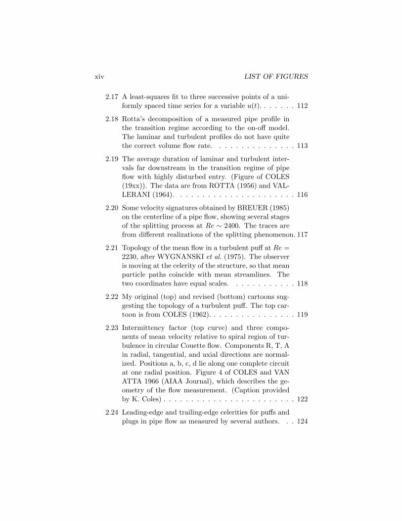
2.17 A least-squares fit to three successive points of a uni-formly spaced time series for a variable u(t). . . . . . . 112

2.18 Rotta’s decomposition of a measured pipe profile inthe transition regime according to the on-off model.The laminar and turbulent profiles do not have quitethe correct volume flow rate. . . . . . . . . . . . . . . 113

2.19 The average duration of laminar and turbulent inter-vals far downstream in the transition regime of pipeflow with highly disturbed entry. (Figure of COLES(19xx)). The data are from ROTTA (1956) and VAL-LERANI (1964). . . . . . . . . . . . . . . . . . . . . . 116

2.20 Some velocity signatures obtained by BREUER (1985)on the centerline of a pipe flow, showing several stagesof the splitting process at Re ∼ 2400. The traces arefrom different realizations of the splitting phenomenon. 117

2.21 Topology of the mean flow in a turbulent puff at Re =2230, after WYGNANSKI et al. (1975). The observeris moving at the celerity of the structure, so that meanparticle paths coincide with mean streamlines. Thetwo coordinates have equal scales. . . . . . . . . . . . 118

2.22 My original (top) and revised (bottom) cartoons sug-gesting the topology of a turbulent puff. The top car-toon is from COLES (1962). . . . . . . . . . . . . . . . 119

2.23 Intermittency factor (top curve) and three compo-nents of mean velocity relative to spiral region of tur-bulence in circular Couette flow. Components R, T, Ain radial, tangential, and axial directions are normal-ized. Positions a, b, c, d lie along one complete circuitat one radial position. Figure 4 of COLES and VANATTA 1966 (AIAA Journal), which describes the ge-ometry of the flow measurement. (Caption providedby K. Coles) . . . . . . . . . . . . . . . . . . . . . . . . 122

2.24 Leading-edge and trailing-edge celerities for puffs andplugs in pipe flow as measured by several authors. . . 124

LIST OF FIGURES xv

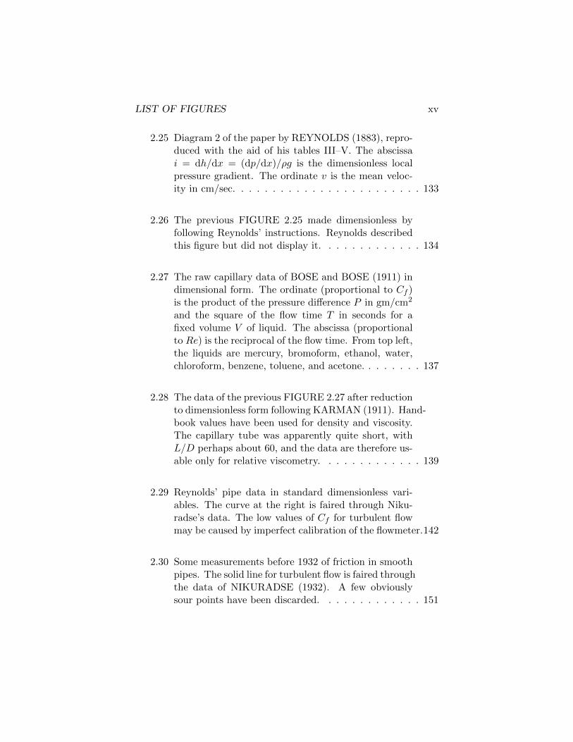
2.25 Diagram 2 of the paper by REYNOLDS (1883), repro-duced with the aid of his tables III–V. The abscissai = dh/dx = (dp/dx)/ρg is the dimensionless localpressure gradient. The ordinate v is the mean veloc-ity in cm/sec. . . . . . . . . . . . . . . . . . . . . . . . 133

2.26 The previous FIGURE 2.25 made dimensionless byfollowing Reynolds’ instructions. Reynolds describedthis figure but did not display it. . . . . . . . . . . . . 134

2.27 The raw capillary data of BOSE and BOSE (1911) indimensional form. The ordinate (proportional to Cf )is the product of the pressure difference P in gm/cm2

and the square of the flow time T in seconds for afixed volume V of liquid. The abscissa (proportionalto Re) is the reciprocal of the flow time. From top left,the liquids are mercury, bromoform, ethanol, water,chloroform, benzene, toluene, and acetone. . . . . . . . 137

2.28 The data of the previous FIGURE 2.27 after reductionto dimensionless form following KARMAN (1911). Hand-book values have been used for density and viscosity.The capillary tube was apparently quite short, withL/D perhaps about 60, and the data are therefore us-able only for relative viscometry. . . . . . . . . . . . . 139

2.29 Reynolds’ pipe data in standard dimensionless vari-ables. The curve at the right is faired through Niku-radse’s data. The low values of Cf for turbulent flowmay be caused by imperfect calibration of the flowmeter.142

2.30 Some measurements before 1932 of friction in smoothpipes. The solid line for turbulent flow is faired throughthe data of NIKURADSE (1932). A few obviouslysour points have been discarded. . . . . . . . . . . . . 151

xvi LIST OF FIGURES

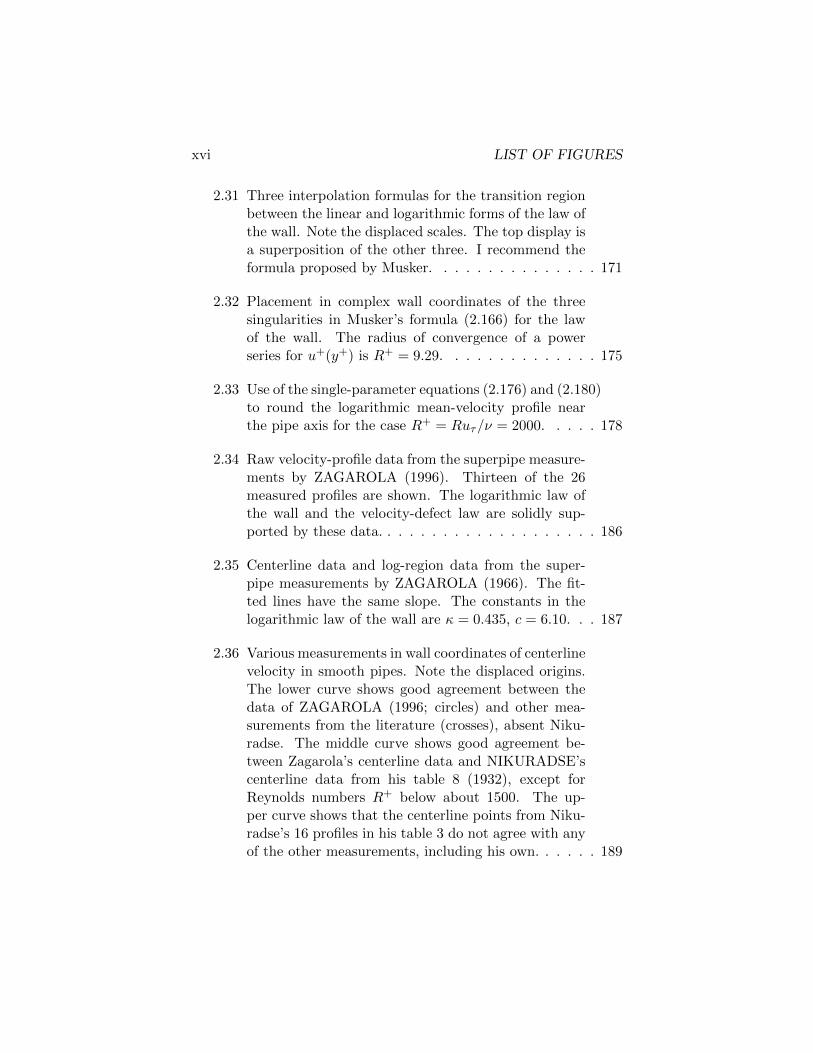
2.31 Three interpolation formulas for the transition regionbetween the linear and logarithmic forms of the law ofthe wall. Note the displaced scales. The top display isa superposition of the other three. I recommend theformula proposed by Musker. . . . . . . . . . . . . . . 171

2.32 Placement in complex wall coordinates of the threesingularities in Musker’s formula (2.166) for the lawof the wall. The radius of convergence of a powerseries for u+(y+) is R+ = 9.29. . . . . . . . . . . . . . 175

2.33 Use of the single-parameter equations (2.176) and (2.180)to round the logarithmic mean-velocity profile nearthe pipe axis for the case R+ = Ruτ/ν = 2000. . . . . 178

2.34 Raw velocity-profile data from the superpipe measure-ments by ZAGAROLA (1996). Thirteen of the 26measured profiles are shown. The logarithmic law ofthe wall and the velocity-defect law are solidly sup-ported by these data. . . . . . . . . . . . . . . . . . . . 186

2.35 Centerline data and log-region data from the super-pipe measurements by ZAGAROLA (1966). The fit-ted lines have the same slope. The constants in thelogarithmic law of the wall are κ = 0.435, c = 6.10. . . 187

2.36 Various measurements in wall coordinates of centerlinevelocity in smooth pipes. Note the displaced origins.The lower curve shows good agreement between thedata of ZAGAROLA (1996; circles) and other mea-surements from the literature (crosses), absent Niku-radse. The middle curve shows good agreement be-tween Zagarola’s centerline data and NIKURADSE’scenterline data from his table 8 (1932), except forReynolds numbers R+ below about 1500. The up-per curve shows that the centerline points from Niku-radse’s 16 profiles in his table 3 do not agree with anyof the other measurements, including his own. . . . . . 189

LIST OF FIGURES xvii

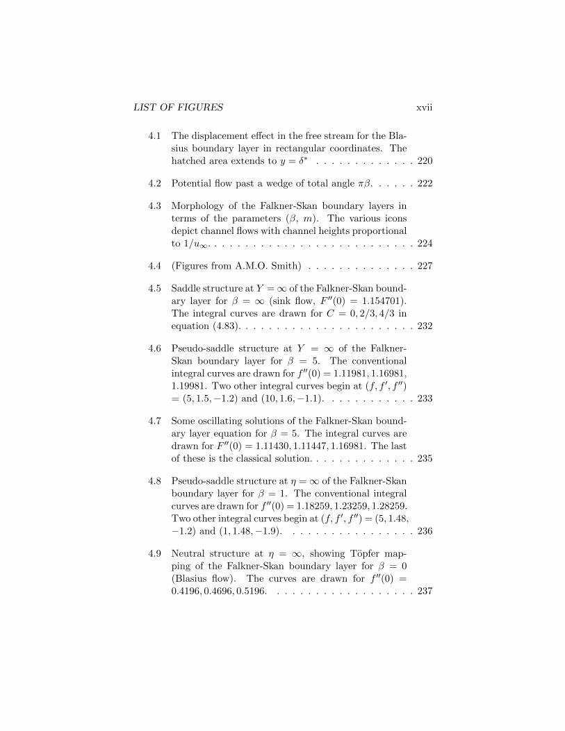
4.1 The displacement effect in the free stream for the Bla-sius boundary layer in rectangular coordinates. Thehatched area extends to y = δ∗ . . . . . . . . . . . . . 220

4.2 Potential flow past a wedge of total angle πβ. . . . . . 222

4.3 Morphology of the Falkner-Skan boundary layers interms of the parameters (β, m). The various iconsdepict channel flows with channel heights proportionalto 1/u∞. . . . . . . . . . . . . . . . . . . . . . . . . . . 224

4.4 (Figures from A.M.O. Smith) . . . . . . . . . . . . . . 227

4.5 Saddle structure at Y =∞ of the Falkner-Skan bound-ary layer for β = ∞ (sink flow, F ′′(0) = 1.154701).The integral curves are drawn for C = 0, 2/3, 4/3 inequation (4.83). . . . . . . . . . . . . . . . . . . . . . . 232

4.6 Pseudo-saddle structure at Y = ∞ of the Falkner-Skan boundary layer for β = 5. The conventionalintegral curves are drawn for f ′′(0) = 1.11981, 1.16981,1.19981. Two other integral curves begin at (f, f ′, f ′′)= (5, 1.5,−1.2) and (10, 1.6,−1.1). . . . . . . . . . . . 233

4.7 Some oscillating solutions of the Falkner-Skan bound-ary layer equation for β = 5. The integral curves aredrawn for F ′′(0) = 1.11430, 1.11447, 1.16981. The lastof these is the classical solution. . . . . . . . . . . . . . 235

4.8 Pseudo-saddle structure at η =∞ of the Falkner-Skanboundary layer for β = 1. The conventional integralcurves are drawn for f ′′(0) = 1.18259, 1.23259, 1.28259.Two other integral curves begin at (f, f ′, f ′′) = (5, 1.48,−1.2) and (1, 1.48,−1.9). . . . . . . . . . . . . . . . . 236

4.9 Neutral structure at η = ∞, showing Topfer map-ping of the Falkner-Skan boundary layer for β = 0(Blasius flow). The curves are drawn for f ′′(0) =0.4196, 0.4696, 0.5196. . . . . . . . . . . . . . . . . . . 237

xviii LIST OF FIGURES

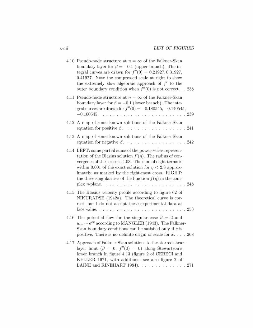
4.10 Pseudo-node structure at η = ∞ of the Falkner-Skanboundary layer for β = −0.1 (upper branch). The in-tegral curves are drawn for f ′′(0) = 0.21927, 0.31927,0.41927. Note the compressed scale at right to showthe extremely slow algebraic approach of f ′ to theouter boundary condition when f ′′(0) is not correct. . 238

4.11 Pseudo-node structure at η = ∞ of the Falkner-Skanboundary layer for β = −0.1 (lower branch). The inte-gral curves are drawn for f ′′(0) =−0.180545,−0.140545,−0.100545. . . . . . . . . . . . . . . . . . . . . . . . . 239

4.12 A map of some known solutions of the Falkner-Skanequation for positive β. . . . . . . . . . . . . . . . . . 241

4.13 A map of some known solutions of the Falkner-Skanequation for negative β. . . . . . . . . . . . . . . . . . 242

4.14 LEFT: some partial sums of the power-series represen-tation of the Blasius solution f ′(η). The radius of con-vergence of the series is 4.03. The sum of eight terms iswithin 0.001 of the exact solution for η < 2.8 approx-imately, as marked by the right-most cross. RIGHT:the three singularities of the function f(η) in the com-plex η-plane. . . . . . . . . . . . . . . . . . . . . . . . 248

4.15 The Blasius velocity profile according to figure 62 ofNIKURADSE (1942a). The theoretical curve is cor-rect, but I do not accept these experimental data atface value. . . . . . . . . . . . . . . . . . . . . . . . . . 253

4.16 The potential flow for the singular case β = 2 andu∞ ∼ ecx according to MANGLER (1943). The Falkner-Skan boundary conditions can be satisfied only if c ispositive. There is no definite origin or scale for x. . . . 268

4.17 Approach of Falkner-Skan solutions to the starred shear-layer limit (β = 0, f ′′(0) = 0) along Stewartson’slower branch in figure 4.13 (figure 2 of CEBECI andKELLER 1971, with additions; see also figure 2 ofLAINE and RINEHART 1984). . . . . . . . . . . . . . 271

LIST OF FIGURES xix

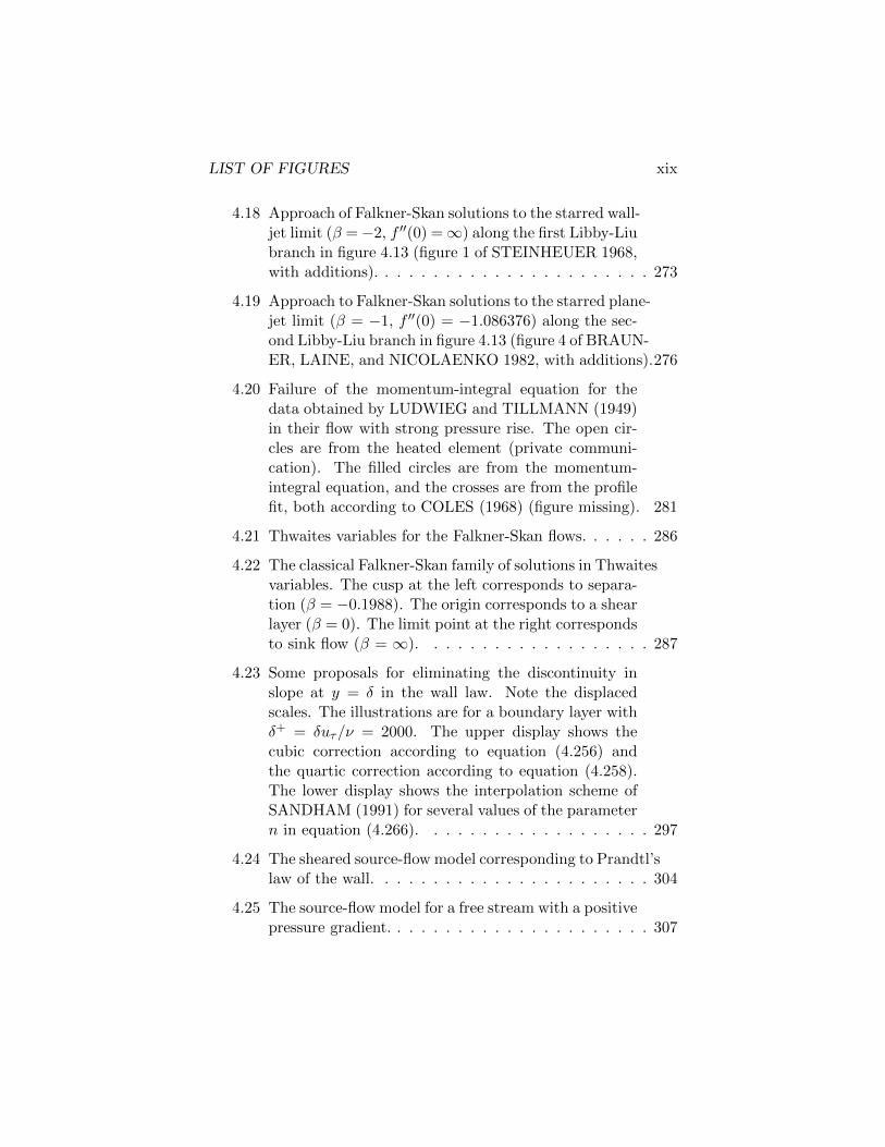
4.18 Approach of Falkner-Skan solutions to the starred wall-jet limit (β =−2, f ′′(0) =∞) along the first Libby-Liubranch in figure 4.13 (figure 1 of STEINHEUER 1968,with additions). . . . . . . . . . . . . . . . . . . . . . . 273

4.19 Approach to Falkner-Skan solutions to the starred plane-jet limit (β = −1, f ′′(0) = −1.086376) along the sec-ond Libby-Liu branch in figure 4.13 (figure 4 of BRAUN-ER, LAINE, and NICOLAENKO 1982, with additions).276

4.20 Failure of the momentum-integral equation for thedata obtained by LUDWIEG and TILLMANN (1949)in their flow with strong pressure rise. The open cir-cles are from the heated element (private communi-cation). The filled circles are from the momentum-integral equation, and the crosses are from the profilefit, both according to COLES (1968) (figure missing). 281

4.21 Thwaites variables for the Falkner-Skan flows. . . . . . 286

4.22 The classical Falkner-Skan family of solutions in Thwaitesvariables. The cusp at the left corresponds to separa-tion (β = −0.1988). The origin corresponds to a shearlayer (β = 0). The limit point at the right correspondsto sink flow (β = ∞). . . . . . . . . . . . . . . . . . . 287

4.23 Some proposals for eliminating the discontinuity inslope at y = δ in the wall law. Note the displacedscales. The illustrations are for a boundary layer withδ+ = δuτ/ν = 2000. The upper display shows thecubic correction according to equation (4.256) andthe quartic correction according to equation (4.258).The lower display shows the interpolation scheme ofSANDHAM (1991) for several values of the parametern in equation (4.266). . . . . . . . . . . . . . . . . . . 297

4.24 The sheared source-flow model corresponding to Prandtl’slaw of the wall. . . . . . . . . . . . . . . . . . . . . . . 304

4.25 The source-flow model for a free stream with a positivepressure gradient. . . . . . . . . . . . . . . . . . . . . . 307

xx LIST OF FIGURES

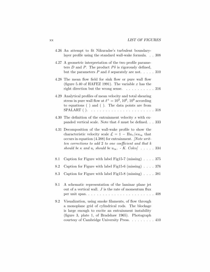
4.26 An attempt to fit Nikuradse’s turbulent boundary-layer profile using the standard wall-wake formula. . . 308

4.27 A geometric interpretation of the two profile parame-ters D and P . The product Pδ is rigorously defined,but the parameters P and δ separately are not. . . . . 310

4.28 The mean flow field for sink flow or pure wall flow(figure 5.40 of HAFEZ 1991). The variable x has theright direction but the wrong sense. . . . . . . . . . . 316

4.29 Analytical profiles of mean velocity and total shearingstress in pure wall flow at δ+ = 103, 106, 109 accordingto equations ( ) and ( ). The data points are fromSPALART ( ). . . . . . . . . . . . . . . . . . . . . . . 318

4.30 The definition of the entrainment velocity s with ex-panded vertical scale. Note that δ must be defined. . . 333

4.31 Decomposition of the wall-wake profile to show thecharacteristic velocity scale L = 1 − Πuτ/κu∞ thatoccurs in equation (4.388) for entrainment. [Note writ-ten corrections to add 2 to one coefficient and that kshould be κ and uι should be u∞. - K. Coles] . . . . . 334

8.1 Caption for Figure with label Fig15-7 (missing) . . . . 375

8.2 Caption for Figure with label Fig15-6 (missing) . . . . 376

8.3 Caption for Figure with label Fig15-8 (missing) . . . . 381

9.1 A schematic representation of the laminar plane jetout of a vertical wall. J is the rate of momentum fluxper unit span. . . . . . . . . . . . . . . . . . . . . . . . 408

9.2 Visualization, using smoke filaments, of flow througha monoplane grid of cylindrical rods. The blockageis large enough to excite an entrainment instability(figure 3, plate 1, of Bradshaw 1965). Photographcourtesy of Cambridge University Press. . . . . . . . . 410

LIST OF FIGURES xxi

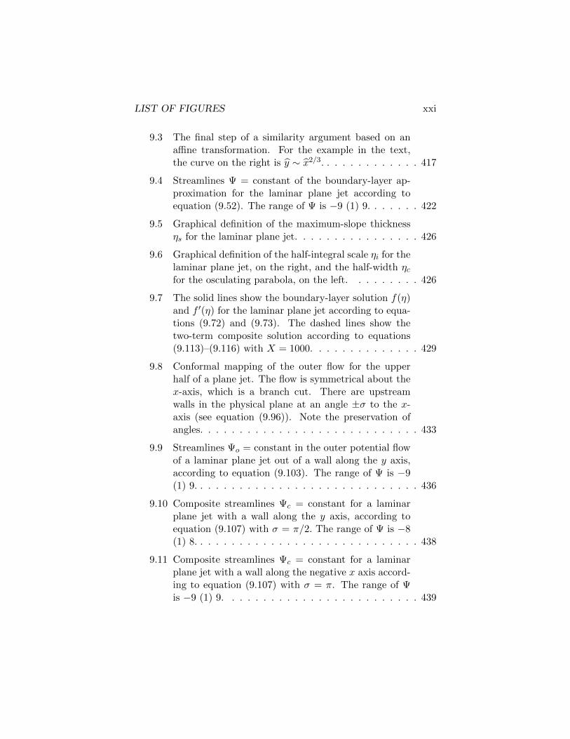
9.3 The final step of a similarity argument based on anaffine transformation. For the example in the text,the curve on the right is y ∼ x2/3. . . . . . . . . . . . . 417

9.4 Streamlines Ψ = constant of the boundary-layer ap-proximation for the laminar plane jet according toequation (9.52). The range of Ψ is −9 (1) 9. . . . . . . 422

9.5 Graphical definition of the maximum-slope thicknessηs for the laminar plane jet. . . . . . . . . . . . . . . . 426

9.6 Graphical definition of the half-integral scale ηi for thelaminar plane jet, on the right, and the half-width ηcfor the osculating parabola, on the left. . . . . . . . . 426

9.7 The solid lines show the boundary-layer solution f(η)and f ′(η) for the laminar plane jet according to equa-tions (9.72) and (9.73). The dashed lines show thetwo-term composite solution according to equations(9.113)–(9.116) with X = 1000. . . . . . . . . . . . . . 429

9.8 Conformal mapping of the outer flow for the upperhalf of a plane jet. The flow is symmetrical about thex-axis, which is a branch cut. There are upstreamwalls in the physical plane at an angle ±σ to the x-axis (see equation (9.96)). Note the preservation ofangles. . . . . . . . . . . . . . . . . . . . . . . . . . . . 433

9.9 Streamlines Ψo = constant in the outer potential flowof a laminar plane jet out of a wall along the y axis,according to equation (9.103). The range of Ψ is −9(1) 9. . . . . . . . . . . . . . . . . . . . . . . . . . . . . 436

9.10 Composite streamlines Ψc = constant for a laminarplane jet with a wall along the y axis, according toequation (9.107) with σ = π/2. The range of Ψ is −8(1) 8. . . . . . . . . . . . . . . . . . . . . . . . . . . . . 438

9.11 Composite streamlines Ψc = constant for a laminarplane jet with a wall along the negative x axis accord-ing to equation (9.107) with σ = π. The range of Ψis −9 (1) 9. . . . . . . . . . . . . . . . . . . . . . . . . 439

xxii LIST OF FIGURES

9.12 Exploratory view of streamlines near the stagnationpoint that appears at X = 0.1925 in the compositeexpansion of a plane laminar jet out of a vertical wall.The streamlines are not equally spaced in Ψ. Thiscurious result is not real; it is an artifact created byuse of the boundary approximation at low Reynoldsnumber. . . . . . . . . . . . . . . . . . . . . . . . . . . 441

9.13 Elements of the linearized jet flap. . . . . . . . . . . . 475

9.14 Detail of the flow near the jet. . . . . . . . . . . . . . . 476

10.1 Schematic connection between the laminar plane freejet and wall jet. . . . . . . . . . . . . . . . . . . . . . . 502

10.2 Streamlines of the boundary-layer model for the lam-inar plane wall jet according to equation (10.71). Therange of........ . . . . . . . . . . . . . . . . . . . . . . . 517

10.3 Mapping of the outer entrained flow for the laminarplane wall jet. . . . . . . . . . . . . . . . . . . . . . . . 521

10.4 Streamlines Ψ = constant of the composite model forthe laminar plane wall jet into a stagnant fluid accord-ing to equation (10.103). . . . . . . . . . . . . . . . . . 523

11.1 Steady laminar plane plume. (Caption provided by B.Coles) . . . . . . . . . . . . . . . . . . . . . . . . . . . 535

12.1 Flow through a screen. (Figure and caption added byK. Coles.) . . . . . . . . . . . . . . . . . . . . . . . . . 552

12.2 Flow in a channel modified by a single shaped screen.(Figure and caption added by K. Coles.) . . . . . . . . 560

A.1 Caption for Figure with label 7.40 (figure on p. 54 ofCOLES 1962). . . . . . . . . . . . . . . . . . . . . . . 572

A.2 Caption for Figure with label 7.41 (figures 10 and 11on p. 56 of COLES 1962). . . . . . . . . . . . . . . . . 573

LIST OF FIGURES xxiii

A.3 Caption for Figure with label 7.43 (figures 12 and 13on p. 58 of COLES 1962). . . . . . . . . . . . . . . . . 573

Preface

AUTHOR’S DRAFT PREFACE

This section was found in an early draft of this monograph. Whileit was not revised after the author added much of the content of thiswork, we include it as it conveys his motivation and approach.– K. Coles

Even limited exposure to industrial problems involving fluid mechan-ics shows that there is a pervasive need for a comprehensive, criticalcompilation of empirical knowledge in the field of turbulent shearflow. The enormous experimental literature published during thelast fifty years, literally thousands of papers, is still mostly undi-gested. This literature is generated in governmental and industrialresearch laboratories and in university departments of aeronautical,chemical, civil, environmental, and mechanical engineering at insti-tutions all over the world. There are also important applications inocean engineering, vehicle and building aerodynamics, dynamic me-teorology and physical oceanography, and even in planetary physicsand astrophysics.

With industrial problems in mind, Anatol Roshko and I havedeveloped over the past 20 years a graduate course in aeronauticsat Caltech called “Technical Fluid Mechanics.” The emphasis isstrongly on turbulent shear flow. The course is normally given everyyear and is well attended. It draws graduate students from severalengineering options other than aeronautics and is also open to se-

xxv

xxvi PREFACE

lected undergraduates who have had at least a first course in fluidmechanics.

For various reasons, none of the existing monographs thatmight be consulted by engineers or used as textbooks in advancedengineering courses on turbulent flow is a satisfactory reference forsuch a course. The most common defect is a lack of adequate ex-perimental content. When I took the decision in 1986 to write thismonograph, much of the lecture material for the course had alreadybeen laboriously collected from the experimental literature, althoughwithout much critical compilation or comparison of data from differ-ent sources. Nevertheless, a large part of the necessary bibliographi-cal preparation and interpretation of data had been carried out, anda solid foundation for a monograph on technical fluid mechanics didexist. To produce this book has involved a substantial commitmentfor several years, once adequate support was obtained for assemblingand collating experimental data.

The fundamental premise for the book is that the only reliableinformation about turbulent flow is experimental information. Thisvaries greatly in quality and completeness, and needs to be carefullyscreened. Some additional premises will be self-evident in the text.First, it is advisable to understand thoroughly the laminar versionof a particular flow, because some conceptual problems are not pe-culiar to turbulent flow; e.g., the third boundary condition for themixing layer, or the integral invariant for the wall jet. Second, themost powerful organizing principle so far available for both laminarand turbulent flow is the principle of similarity. Third, the mostimportant phenomenological concept for many turbulent flows is theconcept of entrainment. The need of the user is often likely to be forhard numbers and practical insights, rather than for elegance. I havetherefore made some use of mixing-length and eddy-viscosity ideas,and even power-law methods, as primitive links between fundamentaland technical problems.

Each chapter of the book deals with one of the classical shearflows (mixing layers, jets, plumes, wakes, boundary layers, pipe flow,and so on ) and with its ramifications, or with an important technicalproblem such as flow management. Wherever possible, the presen-

xxvii

tation is intended to suggest how various flow problems might beconnected analytically and experimentally one to another, using asfar as possible a consistent notation and a consistent level of rigorand detail.

In practically all cases, I have organized and presented the datain the language of the Reynolds-averaged equations of motion, sincethere is general agreement that these equations, although incomplete,are at least correct. The important areas of turbulence modeling andnumerical simulation are served indirectly, by extensive documenta-tion of the experimental facts that modeling and simulation attemptto reproduce. I have made every effort to ensure that the mate-rial of the monograph will not quickly become dated. The rapidlyevolving subject of coherent structure is therefore discussed only incases where the Reynolds-averaged equations clearly do not sufficefor describing the phenomenology of particular turbulent flows. Anexample is the sublayer of a turbulent flow near a smooth wall.

Finally, I found it essential to limit the objectives of the book.Combustion is not discussed. Neither is the very large subject ofcompressibility, including aerodynamic noise. Transition is viewedprimarily from the turbulent side, with the elements of randomnessand three-dimensionality already present. Effects of body forces as-sociated with buoyancy or curvature are discussed, but not in thecontext of the classical Benard or Couette flows. Grid turbulence ismentioned mainly in connection with flow management. Instrumen-tation and experimental techniques are discussed mainly in connec-tion with questions of good experimental practice.

The list of references cited in this monograph is extensive butnot exhaustive. The list is most complete when my objective is toassemble and compare the experimental evidence on some specialtopic. In the face of a large volume of material, my task has beenmade easier by the evolution of the scientific literature from archivaljournals to abstract journals to survey and review volumes. I havemade heavy use of Science Citation Index and of the surveys thatare a common component of Ph.D. theses. I have also used the seriesof unpublished reports prepared by various groups of experts for thesecond (1980-1981) Stanford conference on computation of turbulent

xxviii PREFACE

flow. Finally, I have taken the time to study most of the originalpapers that have laid the foundations of fluid mechanics since themiddle of the 19th century. This study changed my ideas about theway that classical contributions to mechanics have been introducedand developed. It also influenced this monograph in a way that Ihope will be seen as respect for the uses of the past.

In a real sense, the part of fluid mechanics treated in this mono-graph is a mature subject. A histogram in time constructed for thereferences cited here shows that paper production is level or decreas-ing. A reasonable inference is that the classical turbulent shear flowsare thought, rightly or wrongly, to be under good control. Activityis shifting to study of coherent structure and to exploitation of thepower of large computing machines. Another area developing slowlybut promising important contributions is the relationship of turbu-lence to dynamical systems theory. I hope that this monograph willbe useful in support of these efforts as well as in solution of engineer-ing problems.

D.C.(July 1995)

EDITOR’S NOTE

The pages that follow represent an attempt to reconstruct the un-finished book left by Donald Coles at his death in May of 2013.Combining a large number of computer files, drafts and printoutsof figures, and various scraps of manuscript and lecture notes hasproven challenging. In places internal clues indicate the intent of theauthor the last time he reviewed or revised a section. The editingwas done between late 2013 and the present by myself and BetsyColes, who also assembled and updated the computer files.

Don Coles often said he wanted to write this work, and overtwenty years ago he began writing to colleagues requesting originalexperimental data so he could replot them in a uniform way. Thetask of creating the plots for figures, with the help of assistants he

xxix

hired, occupied the great majority of time and effort in the author’slater years. His intention to complete the figures before turning hisattention to revising the respective chapters accounts for the frag-mentary state of parts of the text.

The working title was “Topics in turbulent shear flow.” Weshortened this title at the suggestion of Prof. Anatol Roshko, whopointed out that the author treats laminar flow, typically at length,before considering corresponding turbulent flows. We did not trackdown many of the references to unspecified sections or figures else-where in the work; some were never created or have not been found.

The manuscript used arbitrary chapter numbers. Some refer-ences (e.g., to missing figures) use these old numbers rather thanthe consecutive chapter numbers of this edition. The author’s typo-graphic conventions, which we have followed where possible, include:

CAPITALS: Names of cited or referenced authors; numbered figuresand tables; cited sections of this work.Boldface: Notes to self, such as items to check or add.Italic: Early draft or tentative material; longer notes about topics tobe covered or material to be included.

Clearly the work is incomplete. Some figures and text may yetturn up in paper files, amounting to 50 to 75 cubic feet, that survive.While it is my intent to survey these, it does not make sense to delaypublication of this work in the name of what will be a lengthy processthat may add little. Similarly, we have not attempted to reconstructa bibliography of the numerous literature references. We would behappy to hear from anyone who cares to compile any of these or whocan suggest errors, omissions, or possible alternate readings of thetext to include in a future edition. In the words of Anatol Roshko, “Itpained [Don] to see anything not done absolutely as well as it couldpossibly be done.” He would be frustrated that this work appears inless than complete and correct form. Nevertheless, we suspect it stillcontains much that may be useful and chose to share what we have.It is time for others to pursue the ideas that lie herein. We simplyask that those who make use of this work credit it by citation in theusual and customary manner of scholars.

xxx PREFACE

We owe thanks to many. Over the years Don Coles was as-sisted by a number of people. We do not have all their names, butthey included Dr. Paul Schatzle, Dr. Misha Pesenson, Dr. GregoryCardell, Jim Edberg, and Evan Coles-Harris. Prof. Emeritus Ana-tol Roshko (Caltech) and Prof. Hassan Nagib (Illinois Tech) gavehelpful input and suggestions. While no dedication survives, we donot need that evidence to know to whom Don Coles would have ded-icated this book: Ellen Coles, the lifelong companion who assistedhim with everything he wrote.

Ken ColesIndiana, PennsylvaniaNovember 2017