RESEARCH ARTICLE

Flow visualization and wall shear stress of a flapping modelhummingbird wing

Erik W. M. Swanton • Blake A. Vanier •

Kamran Mohseni

Received: 13 March 2009 / Revised: 1 October 2009 / Accepted: 20 January 2010

� Springer-Verlag 2010

Abstract The unsteady low Reynolds number aerody-

namics of flapping flight was investigated experimentally

through flow visualization by suspended particle imagery

and wall shear stress measurement from micro-array

hot-film anemometry. In conjunction, a mechanism was

developed to create a flapping motion with three degrees of

freedom and adjustable flapping frequency. The flapping

kinematics and wing shape were selected for dynamic

similarity to a hummingbird during hovering flight. Flow

visualization was used to validate the anemometry obser-

vations of leading edge vortex (LEV) characteristics and

to investigate the necessity of spanwise flow in LEV sta-

bility. The shear sensors determined LEV characteristics

throughout the translation section of the stroke period for

various wing speeds. It was observed that a minimum fre-

quency between 2 and 3.5 Hz is required for the formation

and stabilization of a LEV. The vortex strength peaked

around 30% of the flapping cycle (corresponding to just past

the translation midpoint), which agrees with results from

previous studies conducted by others. The shear sensors

also indicated a mild growth in LEV size during translation

sections of the wing’s motion. This growth magnitude was

nearly constant through a range of operating frequencies.

1 Introduction

Although most researchers agree that existence of an

attached leading edge vortex (LEV) is a significant con-

tributor to the strong lift forces observed in flapping fliers,

the structure and stability methods of attached vorticity are

still a point of controversy (Birch and Dickinson 2001;

Bomphrey et al. 2005; van den Berg and Ellington 1997a,

b; Srygley and Thomas 2002). Specifically, three major

characteristics of the flow are questioned: growth of the

separation bubble during each half-stroke, location and

continuity of the LEV, and presence of axial flow.

Many studies have concluded that attachment of the

LEV throughout translation implies that a dynamic stall

condition is produced, which has been known to induce

large lift forces in fixed-wing aircraft (Sane 2003). One of

the first studies to investigate attached vorticity in flapping

flight was by Maxworthy who was attempting to expand on

the ‘clap and fling’ mechanisms that had been observed in

wasps (Weis-Fogh 1973; Maxworthy 1979). During the

‘fling’ motion, he observed LEV structures that merged

into tip vortices and root vortices at the ends of each wing.

Both the tip and root vortices swept back and connected

with the LEV from the opposing wing to create a contin-

uous complex loop. The vortices remained attached and

stable through the entire downstroke, explaining the

underestimates of lift production by inviscid models. He

also described a helical structure of the LEV where sig-

nificant axial flow near the leading edge transported vor-

ticity from the LEV core to the wingtips; thereby inhibiting

the shedding that would be expected in a two-dimensional

analysis.

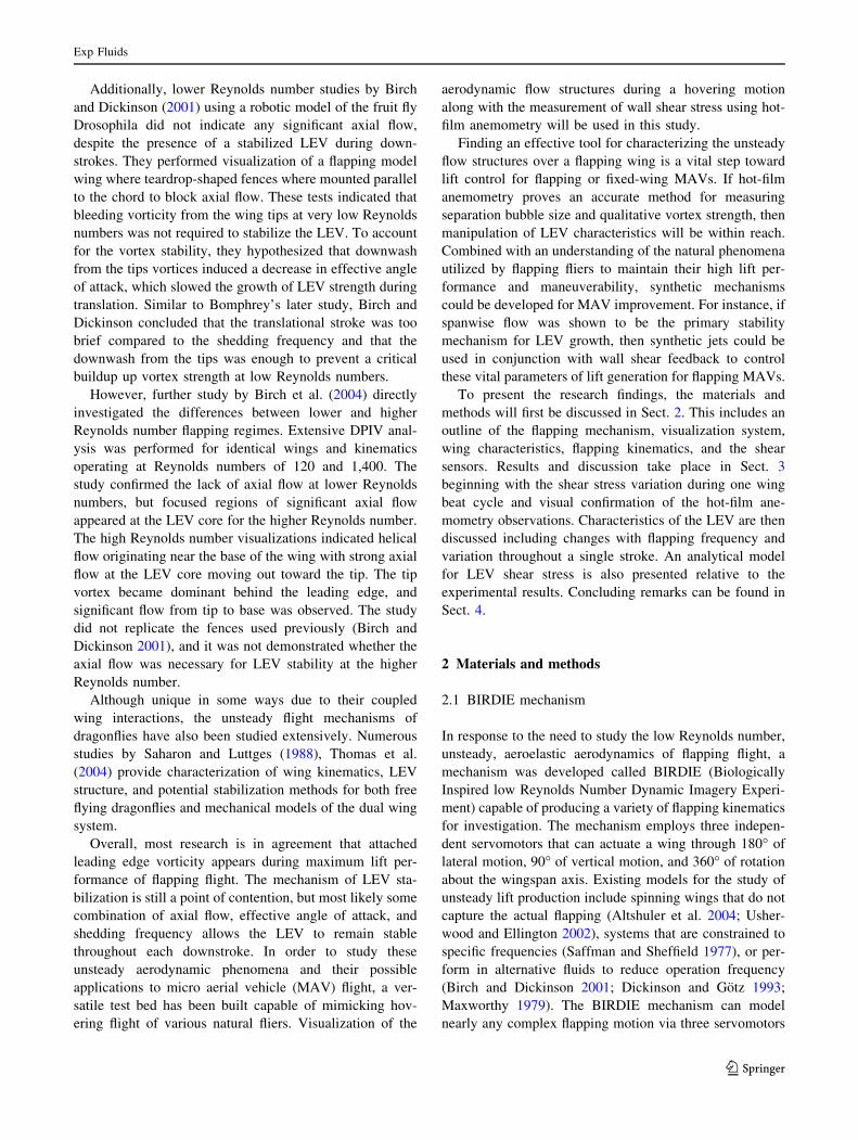
More recently, van den Berg and Ellington visualized

flow around a mechanical model of the flying hawkmoth,

Manduca sexta, and demonstrated a similar LEV forming

at the base of the wing and spiraling outward to join the tip

vortices (Fig. 1) (van den Berg and Ellington 1997b). The

LEV was helical over the wing with significant axial flow

moving from a surface bound focus at the base to the

connected tip vortex that swept backward (Fig. 2b). This

E. W. M. Swanton � B. A. Vanier � K. Mohseni (&)

Department of Aerospace Engineering Sciences,

University of Colorado, Boulder, CO 80309-429, USA

e-mail: mohseni@colorado.edu

123

Exp Fluids

DOI 10.1007/s00348-010-0832-1

corroborates the observations by Maxworthy, except that

Ellington’s single wing hovering motion could not simulate

interaction with an opposing wing and thus did not recreate

Maxworthy’s connected root vortices. By observing smoke

blobs released from the base of the wing, axial flow

velocity at the middle of the wing was calculated as high as

the mean velocity of the wing tip. This strong axial flow

was proposed as the mechanism for maintaining the sta-

bility of LEV by bleeding energy out into the tip vortex.

This similar conclusion was reached despite the order of

magnitude increase in Reynolds number compared to

Maxworthy’s model.

While other researchers have similarly observed stable

LEV structures attached to flapping wings, some have not

noted the same prominent axial flow. For example, Bom-

phrey has questioned the role of axial flow in LEV sta-

bilization using DPIV and smoke visualizations of a

tethered hawkmoth (Bomphrey et al. 2005). The LEV was

observed, but not in the helical form noted by Ellington. In

fact, the LEV maintained relatively constant diameter

across the entire leading edge and was continuous across

the thorax (Fig. 2a). Axial flow components were not

measured, but it was deduced that if axial velocity was

present in the flow, it must have been \15% of the tip

velocity. At this maximum value, it would be a signifi-

cantly smaller percentage than the relative axial velocity

found in delta-winged aircraft experiencing dynamic stall.

Bomphrey suggests that the Strouhal number of the flight

regime is such that vorticity does not build fast enough to

be shed before the end of each stroke.

A wide variety of flapping insects have been similarly

studied. Flow visualization performed by Srygley and

Thomas of free flying red admiral butterflies, Vanessa

atalanta, did not exhibit helical LEV structures, significant

spanwise flow, or the increasing vortex size that is char-

acteristic of a dynamic stall condition (Srygley and Thomas

2002). The LEV did not grow significantly throughout each

stroke and was continuous across the thorax (Fig. 2a). This

equilibrium without axial flow indicated that something

else must be stabilizing the vortex. Additionally, the but-

terflies employed an array of unsteady aerodynamic lift

mechanisms, and an attached LEV did not appear during

every stroke but only when high lift was required. Because

the butterflies were flying freely in a 1.5 ms-1 flow instead

of hovering, maximum lift was unnecessary and would

have caused excessive drag. Srygley and Thomas postu-

lated that the consistent LEV observed in tethered

Hawkmoths was an artifact of the tethering and that they

would likely not employ that technique during free

hovering flight.

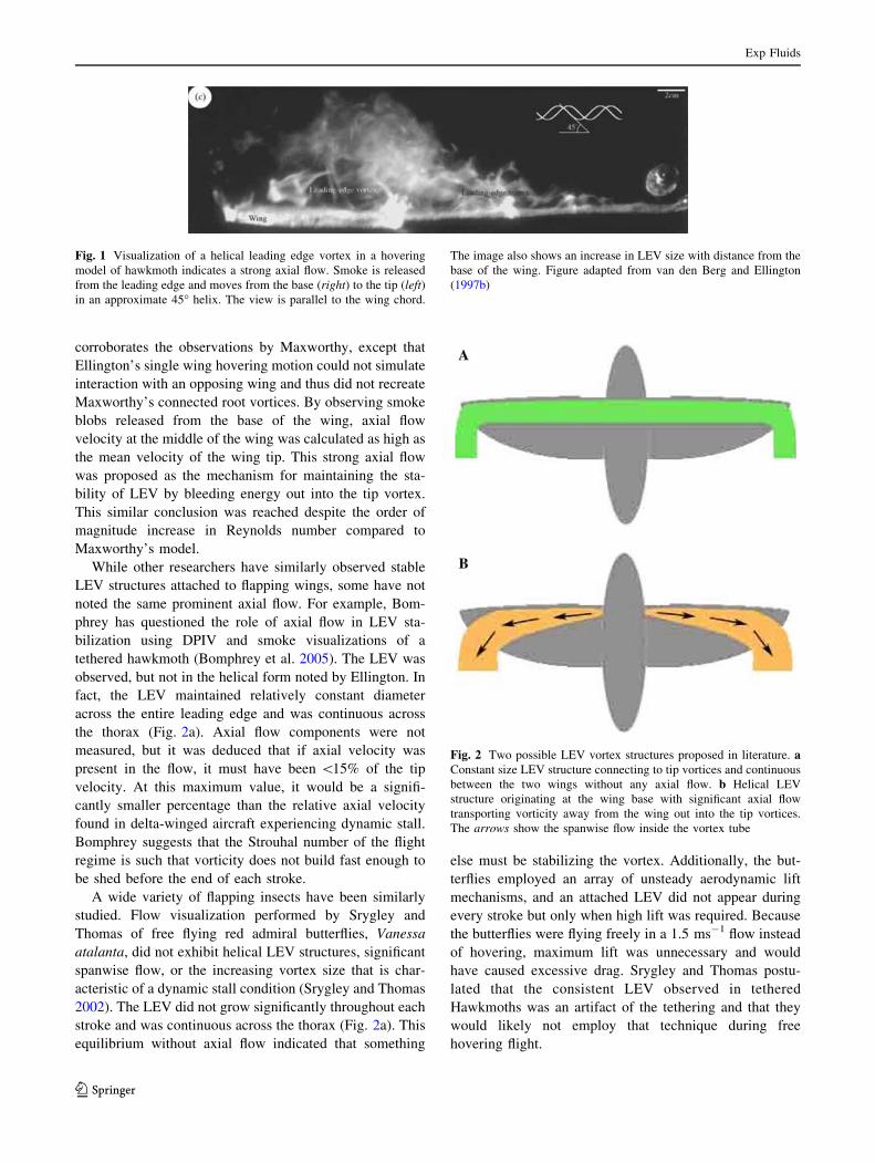
Fig. 1 Visualization of a helical leading edge vortex in a hovering

model of hawkmoth indicates a strong axial flow. Smoke is released

from the leading edge and moves from the base (right) to the tip (left)in an approximate 45� helix. The view is parallel to the wing chord.

The image also shows an increase in LEV size with distance from the

base of the wing. Figure adapted from van den Berg and Ellington

(1997b)

Fig. 2 Two possible LEV vortex structures proposed in literature. aConstant size LEV structure connecting to tip vortices and continuous

between the two wings without any axial flow. b Helical LEV

structure originating at the wing base with significant axial flow

transporting vorticity away from the wing out into the tip vortices.

The arrows show the spanwise flow inside the vortex tube

Exp Fluids

123

Additionally, lower Reynolds number studies by Birch

and Dickinson (2001) using a robotic model of the fruit fly

Drosophila did not indicate any significant axial flow,

despite the presence of a stabilized LEV during down-

strokes. They performed visualization of a flapping model

wing where teardrop-shaped fences where mounted parallel

to the chord to block axial flow. These tests indicated that

bleeding vorticity from the wing tips at very low Reynolds

numbers was not required to stabilize the LEV. To account

for the vortex stability, they hypothesized that downwash

from the tips vortices induced a decrease in effective angle

of attack, which slowed the growth of LEV strength during

translation. Similar to Bomphrey’s later study, Birch and

Dickinson concluded that the translational stroke was too

brief compared to the shedding frequency and that the

downwash from the tips was enough to prevent a critical

buildup up vortex strength at low Reynolds numbers.

However, further study by Birch et al. (2004) directly

investigated the differences between lower and higher

Reynolds number flapping regimes. Extensive DPIV anal-

ysis was performed for identical wings and kinematics

operating at Reynolds numbers of 120 and 1,400. The

study confirmed the lack of axial flow at lower Reynolds

numbers, but focused regions of significant axial flow

appeared at the LEV core for the higher Reynolds number.

The high Reynolds number visualizations indicated helical

flow originating near the base of the wing with strong axial

flow at the LEV core moving out toward the tip. The tip

vortex became dominant behind the leading edge, and

significant flow from tip to base was observed. The study

did not replicate the fences used previously (Birch and

Dickinson 2001), and it was not demonstrated whether the

axial flow was necessary for LEV stability at the higher

Reynolds number.

Although unique in some ways due to their coupled

wing interactions, the unsteady flight mechanisms of

dragonflies have also been studied extensively. Numerous

studies by Saharon and Luttges (1988), Thomas et al.

(2004) provide characterization of wing kinematics, LEV

structure, and potential stabilization methods for both free

flying dragonflies and mechanical models of the dual wing

system.

Overall, most research is in agreement that attached

leading edge vorticity appears during maximum lift per-

formance of flapping flight. The mechanism of LEV sta-

bilization is still a point of contention, but most likely some

combination of axial flow, effective angle of attack, and

shedding frequency allows the LEV to remain stable

throughout each downstroke. In order to study these

unsteady aerodynamic phenomena and their possible

applications to micro aerial vehicle (MAV) flight, a ver-

satile test bed has been built capable of mimicking hov-

ering flight of various natural fliers. Visualization of the

aerodynamic flow structures during a hovering motion

along with the measurement of wall shear stress using hot-

film anemometry will be used in this study.

Finding an effective tool for characterizing the unsteady

flow structures over a flapping wing is a vital step toward

lift control for flapping or fixed-wing MAVs. If hot-film

anemometry proves an accurate method for measuring

separation bubble size and qualitative vortex strength, then

manipulation of LEV characteristics will be within reach.

Combined with an understanding of the natural phenomena

utilized by flapping fliers to maintain their high lift per-

formance and maneuverability, synthetic mechanisms

could be developed for MAV improvement. For instance, if

spanwise flow was shown to be the primary stability

mechanism for LEV growth, then synthetic jets could be

used in conjunction with wall shear feedback to control

these vital parameters of lift generation for flapping MAVs.

To present the research findings, the materials and

methods will first be discussed in Sect. 2. This includes an

outline of the flapping mechanism, visualization system,

wing characteristics, flapping kinematics, and the shear

sensors. Results and discussion take place in Sect. 3

beginning with the shear stress variation during one wing

beat cycle and visual confirmation of the hot-film ane-

mometry observations. Characteristics of the LEV are then

discussed including changes with flapping frequency and

variation throughout a single stroke. An analytical model

for LEV shear stress is also presented relative to the

experimental results. Concluding remarks can be found in

Sect. 4.

2 Materials and methods

2.1 BIRDIE mechanism

In response to the need to study the low Reynolds number,

unsteady, aeroelastic aerodynamics of flapping flight, a

mechanism was developed called BIRDIE (Biologically

Inspired low Reynolds Number Dynamic Imagery Experi-

ment) capable of producing a variety of flapping kinematics

for investigation. The mechanism employs three indepen-

dent servomotors that can actuate a wing through 180� of

lateral motion, 90� of vertical motion, and 360� of rotation

about the wingspan axis. Existing models for the study of

unsteady lift production include spinning wings that do not

capture the actual flapping (Altshuler et al. 2004; Usher-

wood and Ellington 2002), systems that are constrained to

specific frequencies (Saffman and Sheffield 1977), or per-

form in alternative fluids to reduce operation frequency

(Birch and Dickinson 2001; Dickinson and Gotz 1993;

Maxworthy 1979). The BIRDIE mechanism can model

nearly any complex flapping motion via three servomotors

Exp Fluids

123

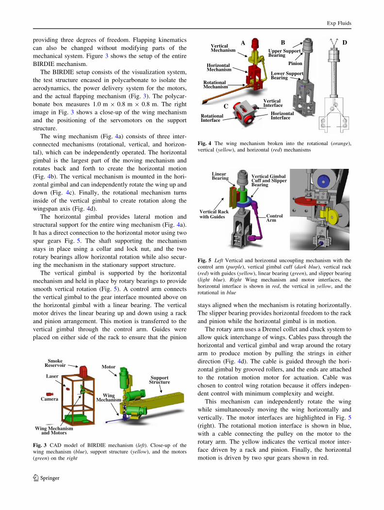
providing three degrees of freedom. Flapping kinematics

can also be changed without modifying parts of the

mechanical system. Figure 3 shows the setup of the entire

BIRDIE mechanism.

The BIRDIE setup consists of the visualization system,

the test structure encased in polycarbonate to isolate the

aerodynamics, the power delivery system for the motors,

and the actual flapping mechanism (Fig. 3). The polycar-

bonate box measures 1.0 m 9 0.8 m 9 0.8 m. The right

image in Fig. 3 shows a close-up of the wing mechanism

and the positioning of the servomotors on the support

structure.

The wing mechanism (Fig. 4a) consists of three inter-

connected mechanisms (rotational, vertical, and horizon-

tal), which can be independently operated. The horizontal

gimbal is the largest part of the moving mechanism and

rotates back and forth to create the horizontal motion

(Fig. 4b). The vertical mechanism is mounted in the hori-

zontal gimbal and can independently rotate the wing up and

down (Fig. 4c). Finally, the rotational mechanism turns

inside of the vertical gimbal to create rotation along the

wingspan axis (Fig. 4d).

The horizontal gimbal provides lateral motion and

structural support for the entire wing mechanism (Fig. 4a).

It has a direct connection to the horizontal motor using two

spur gears Fig. 5. The shaft supporting the mechanism

stays in place using a collar and lock nut, and the two

rotary bearings allow horizontal rotation while also secur-

ing the mechanism in the stationary support structure.

The vertical gimbal is supported by the horizontal

mechanism and held in place by rotary bearings to provide

smooth vertical rotation (Fig. 5). A control arm connects

the vertical gimbal to the gear interface mounted above on

the horizontal gimbal with a linear bearing. The vertical

motor drives the linear bearing up and down using a rack

and pinion arrangement. This motion is transferred to the

vertical gimbal through the control arm. Guides were

placed on either side of the rack to ensure that the pinion

stays aligned when the mechanism is rotating horizontally.

The slipper bearing provides horizontal freedom to the rack

and pinion while the horizontal gimbal is in motion.

The rotary arm uses a Dremel collet and chuck system to

allow quick interchange of wings. Cables pass through the

horizontal and vertical gimbal and wrap around the rotary

arm to produce motion by pulling the strings in either

direction (Fig. 4d). The cable is guided through the hori-

zontal gimbal by grooved rollers, and the ends are attached

to the rotation motion motor for actuation. Cable was

chosen to control wing rotation because it offers indepen-

dent control with minimum complexity and weight.

This mechanism can independently rotate the wing

while simultaneously moving the wing horizontally and

vertically. The motor interfaces are highlighted in Fig. 5

(right). The rotational motion interface is shown in blue,

with a cable connecting the pulley on the motor to the

rotary arm. The yellow indicates the vertical motor inter-

face driven by a rack and pinion. Finally, the horizontal

motion is driven by two spur gears shown in red.

Camera

SmokeReservoir

Wing Mechanism and Motors

WingMechanism

Motor

SupportStructure

Laser

Fig. 3 CAD model of BIRDIE mechanism (left). Close-up of the

wing mechanism (blue), support structure (yellow), and the motors

(green) on the right

VerticalMechanism

Horizontal Mechanism

RotationalMechanism

A D

RotationalInterface

VerticalInterface

HorizontalInterface

C

BUpper SupportBearing

Lower SupportBearing

Pinion

Fig. 4 The wing mechanism broken into the rotational (orange),

vertical (yellow), and horizontal (red) mechanisms

Vertical Rack with Guides

LinearBearing Vertical Gimbal

Cuff and SlipperBearing

ControlArm

Fig. 5 Left Vertical and horizontal uncoupling mechanism with the

control arm (purple), vertical gimbal cuff (dark blue), vertical rack

(red) with guides (yellow), linear bearing (green), and slipper bearing

(light blue). Right Wing mechanism and motor interfaces, the

horizontal interface is shown in red, the vertical in yellow, and the

rotational in blue

Exp Fluids

123

2.2 Visualization

To determine the geometry and stability of the LEV, sus-

pended particle imagery (SPI) was employed using fine

particulate oil smoke and high-speed videography. Smoke

was delivered from a diffuser above the wing, creating a

laminar stream of particulates across the test section.

As the wing passed through the smoke, a thin section of

the wing was illuminated by a laser beam split with a

beveled line-generating lens. For adequate power, an Aixiz

Service and International AIX-532-1000 laser was used

operating at a 532 nm wavelength and 1,000 mW. The lens

was an Edmond Optics line generator with a divergence of

15� to minimize variation of the laser sheet with distance.

The PS31ST Oil Based Smoke Generator provided very

fine particles (0.2–0.3 micron diameter), high reflectivity,

and no residue on the wing. See Fig. 6 for an image of the

test setup.

Images of the visualization were gathered using a Vision

Research Phantom v4.3 color high-speed camera operating

between 500 and 1,200 fps depending on the flapping

frequency.

2.3 Model wing and kinematics

Although insects are the most common animals capable of

hovering flight, hummingbirds may provide an improved

basis for investigation into MAV design due to their size,

maneuverability, and lift capabilities. However, to achieve

a reproducible mechanism that loosely mimics humming-

bird flight, some simplifications were used to create the

model wing and its associated movement. The model wing

is a simple rectangular shape shown in Fig. 7, with a span

of 15 cm and a chord length of 4 cm. The aspect ratio was

chosen according to the average wing dimensions of the

Rufus hummingbird (Tobalske et al. 2007). The matte

white border was thinly painted onto the wing to increase

the visibility of the edge during motion. The structure was

made of a carbon fiber spar wrapped in bidirectional carbon

fiber weave to produce a stiff yet light wing platform. The

high stiffness was intended to reduce the possible effects of

wing tip deflection. Although wing twisting and tip

deflection are utilized by free flying hummingbirds, espe-

cially during pitch and roll maneuvers, a stiff wing was

chosen to reduce the complexities of the model and focus

on LEV stability (Warrick et al. 2005). The hot-film ane-

mometry sensor is mounted near the base of the wing. For

continuity throughout testing, all the cross-sectional

structure comparisons were made 50 mm from the base of

the wing (Fig. 7).

For simplicity, the mechanism was programmed so that

the leading edge traced a basic figure eight shape if viewed

in a plane perpendicular to the span axis. While not strictly

a reproduction of hummingbird wing kinematics, the

motion resembles the general hovering stroke parameters

of most natural fliers.

The periodic figure eight motion was modeled using

three sinusoidal functions where the vertical motion was

twice the frequency of the horizontal and rotational motion

(Fig. 8). The actual parameters of motion for the model

were chosen based on a study of the wing kinematics of a

hummingbird during hovering flight (Tobalske et al. 2007).

The motion amplitudes used during testing were 70� hor-

izontally, 20� vertically, and 70� rotationally about the

wing axis. This provided a 20� geometric angle of attack

during mid-downstroke, a stroke amplitude of 140�, and a

Fig. 6 Visualization test setup.

The reservoir above feeds

smoke through the diffuser to

the test section where the wing

is located. Below the test

section is a second diffuser with

a low suction exhaust. The

image is viewed from the same

position as the high-speed

camera, with the laser

positioned on the right and

aimed into the structure

Exp Fluids

123

maximum stroke deviation of 20� (Sane and Dickinson

2001). For analysis of the accuracy of the mechanism in

producing the proposed motion, see the work by Vanier

(2008).

For hovering flight in three dimensions, using the wing

tip as the reference and accounting for both the span and

the cord, the Reynolds number is defined as (Shyy et al.

2008):

Ref 3 ¼/f R2

m4

AR

� �; ð1Þ

where / is the amplitude of the horizontal wing motion in

radians (see Fig. 8), f is the frequency, R is the wing length,

m is the kinematic viscosity, AR is the aspect ratio, where

AR = (2R)2/S, and S is the total surface area of the wings,

and the subscript Ref3 represents the Reynolds number for a

3D flapping wing in hovering flight. For this study, Rey-

nolds numbers ranged from *1,000 to 5,100, or very

nearly 1,000 times the experimental flapping frequency.

2.4 Wall shear sensors

To provide feedback that can assist in the control of flap-

ping flight, a sensor was selected capable of characterizing

the aerodynamic flow structures over the wing. Hot-film

anemometry provides a light but sensitive means of

determining the size of the leading edge separation bubble

through estimation of flow reattachment along the wing

chord. Monitoring the evolution of the separation bubble

and wall shear provides insight into lift production and

therefore could enable flight control.

2.4.1 Hot-film calibration

The preliminary focus of the hot-film sensors is to detect

LEV existence and any variation in the flow reattachment

point; therefore, an absolute calibration is not necessary. A

relative calibration of the sensors is adequate because the

voltage signal from the circuit directly relates to the flow

conditions. The calibration was performed by subjecting

the sensors to a reference flow and then normalizing the

subsequent voltage responses. All sensors are normalized

relative to one reference sensor, in our case hot-film sensor

number five. This ensures a similar response of each sen-

sor, accounting for the differences in each element and the

components in each constant temperature circuit. These

voltages can then be used to determine the wall shear stress

at any location relative to the reference hot-film sensor.

In order to generate consistent flow conditions for a

normalization of the elements, a small tube provided a

steady flow velocity. With the wing and sensor array

secured on a platform, slides were placed to allow smooth

platform movement along a fixed path. The tube was then

positioned with an adjustable vice so that its exit aimed

along the sensor array with a shallow angle, just a few

millimeters off the wing surface.

The activated sensor array was guided under the tube at

a constant velocity, the data were logged, and the proce-

dure repeated while alternating between the front and rear

sensors entering the calibration flow first. A sample result

of the sensor output voltage during the calibration process

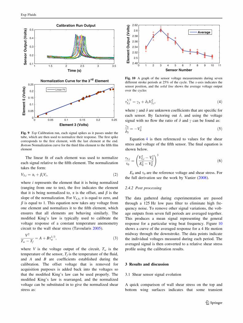
is shown in Fig. 9.

Once the output spikes are captured, the baseline voltage

response (with no applied airflow) is subtracted from the

signal to obtain the pure response. The values are then

plotted against the fifth sensor response to determine a

relative scaling factor using a linear regression shown in

Fig. 9.

40 mm

150 mm

50 mm

9.5 mm

32 mm

Sensor 1

Sensor 10

SensingElements

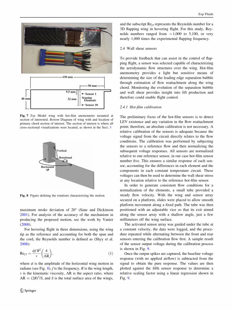
Fig. 7 Top Model wing with hot-film anemometer mounted at

section of interested. Bottom Diagram of wing with and location of

primary chord section of interest. The section of interest is where all

cross-sectional visualizations were located, as shown in the Sect. 3

Horizontal(φφ)

Vertical

Rotational

Fig. 8 Figure defining the rotations characterizing the motion

Exp Fluids

123

The linear fit of each element was used to normalize

each signal relative to the fifth element. The normalization

takes the form:

V5;i ¼ ai þ biVi; ð2Þ

where i represents the element that it is being normalized

(ranging from one to ten), the five indicates the element

that it is being normalized to, a is the offset, and b is the

slope of the normalization. For V5,5, a is equal to zero, and

b is equal to 1. This equation now takes any voltage from

one element and normalizes it to the fifth element, which

ensures that all elements are behaving similarly. The

modified King’s law is typically used to calibrate the

voltage response of a constant temperature anemometry

circuit to the wall shear stress (Tavoularis 2005).

V2

Tw � Tf¼ Aþ Bs1=3

w ; ð3Þ

where V is the voltage output of the circuit, Tw is the

temperature of the sensor, Tf is the temperature of the fluid,

and A and B are coefficients established during the

calibration. The offset voltage that is removed for

acquisition purposes is added back into the voltages so

that the modified King’s law can be used properly. The

modified King’s law is rearranged, and the normalized

voltage can be substituted in to give the normalized shear

stress as:

s1=35;i ¼ c5 þ d5V2

5;i; ð4Þ

where c and d are unknown coefficients that are specific for

each sensor. By factoring out d, and using the voltage

signal with no flow the ratio of d and c can be found as:

c5

d5

¼ �V20 ð5Þ

Equation 4 is then referenced to values for the shear

stress and voltage of the fifth sensor. The final equation is

shown below.

s5;i

s0

¼V2

5;i � V20

E20 � V2

0

!3

ð6Þ

E0 and s0 are the reference voltage and shear stress. For

the full derivation see the work by Vanier (2008).

2.4.2 Post processing

The data gathered during experimentation are passed

through a 125 Hz low pass filter to eliminate high fre-

quency noise. To remove other signal variations, the volt-

age outputs from seven full periods are averaged together.

This produces a mean signal representing the general

response for a particular wing beat frequency. Figure 10

shows a curve of the averaged response for a 4 Hz motion

midway through the downstroke. The data points indicate

the individual voltages measured during each period. The

averaged signal is then converted to a relative shear stress

profile using the calibration results.

3 Results and discussion

3.1 Shear sensor signal evolution

A quick comparison of wall shear stress on the top and

bottom wing surfaces indicates that some transient

0 0.05 0.1 0.15 0.2 0.250

0.05

0.1

0.15

0.2

0.25

Element 3 (Volts)

Ele

men

t 5

(Vo

lts)

Normalization Curve for the 3rd Element

Linear Fit

1 1.5 2 2.5 3 3.50.1

0.2

0.3

0.4

0.5

Time (s)

Sen

sor

Ou

tpu

t (V

olt

s)Calibration Run Output

Fig. 9 Top Calibration run, each signal spikes as it passes under the

tube, which are then used to normalize their response. The first spike

corresponds to the first element, with the last element at the end.

Bottom Normalization curve for the third film element to the fifth film

element

0 1 2 3 4 5 6 7 8 9 10 112.48

2.5

2.52

2.54

2.56

2.58

2.6

2.62

Sensor Number

Ele

men

t O

utp

ut

(Vo

lts)

Average

Fig. 10 A graph of the sensor voltage measurements during seven

different stroke periods at 25% of the cycle. The x-axis indicates the

sensor position, and the solid line shows the average voltage output

over the cycles

Exp Fluids

123

phenomenon occurs over the top of the wing through each

downstroke (Fig. 11). During the half-cycle with the sensor

on top of the wing, a large increase in shear stress is

observed, which disappears as the wing decelerates at the

end of the stroke. This is likely due to formation of the

LEV, since trapped vorticity above the wing would locally

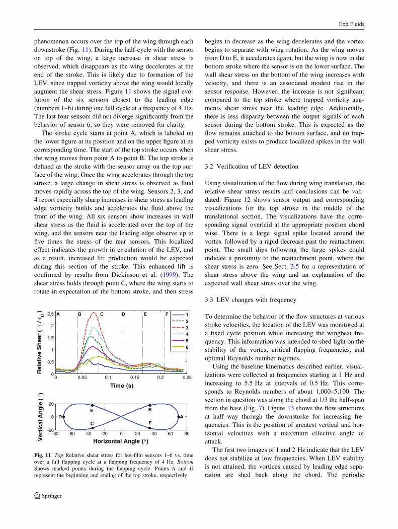
augment the shear stress. Figure 11 shows the signal evo-

lution of the six sensors closest to the leading edge

(numbers 1–6) during one full cycle at a frequency of 4 Hz.

The last four sensors did not diverge significantly from the

behavior of sensor 6, so they were removed for clarity.

The stroke cycle starts at point A, which is labeled on

the lower figure at its position and on the upper figure at its

corresponding time. The start of the top stroke occurs when

the wing moves from point A to point B. The top stroke is

defined as the stroke with the sensor array on the top sur-

face of the wing. Once the wing accelerates through the top

stroke, a large change in shear stress is observed as fluid

moves rapidly across the top of the wing. Sensors 2, 3, and

4 report especially sharp increases in shear stress as leading

edge vorticity builds and accelerates the fluid above the

front of the wing. All six sensors show increases in wall

shear stress as the fluid is accelerated over the top of the

wing, and the sensors near the leading edge observe up to

five times the stress of the rear sensors. This localized

effect indicates the growth in circulation of the LEV, and

as a result, increased lift production would be expected

during this section of the stroke. This enhanced lift is

confirmed by results from Dickinson et al. (1999). The

shear stress holds through point C, where the wing starts to

rotate in expectation of the bottom stroke, and then stress

begins to decrease as the wing decelerates and the vortex

begins to separate with wing rotation. As the wing moves

from D to E, it accelerates again, but the wing is now in the

bottom stroke where the sensor is on the lower surface. The

wall shear stress on the bottom of the wing increases with

velocity, and there is an associated modest rise in the

sensor response. However, the increase is not significant

compared to the top stroke where trapped vorticity aug-

ments shear stress near the leading edge. Additionally,

there is less disparity between the output signals of each

sensor during the bottom stroke. This is expected as the

flow remains attached to the bottom surface, and no trap-

ped vorticity exists to produce localized spikes in the wall

shear stress.

3.2 Verification of LEV detection

Using visualization of the flow during wing translation, the

relative shear stress results and conclusions can be vali-

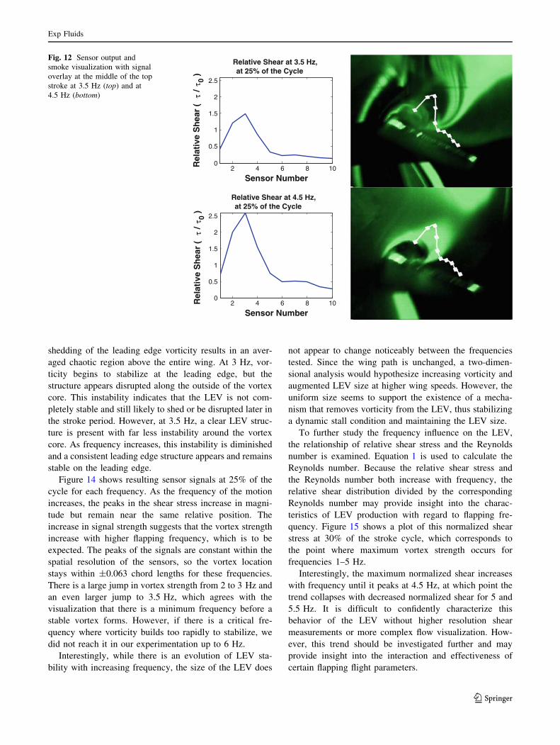
dated. Figure 12 shows sensor output and corresponding

visualizations for the top stroke in the middle of the

translational section. The visualizations have the corre-

sponding signal overlaid at the appropriate position chord

wise. There is a large signal spike located around the

vortex followed by a rapid decrease past the reattachment

point. The small dips following the large spikes could

indicate a proximity to the reattachment point, where the

shear stress is zero. See Sect. 3.5 for a representation of

shear stress above the wing and an explanation of the

expected wall shear stress over the wing.

3.3 LEV changes with frequency

To determine the behavior of the flow structures at various

stroke velocities, the location of the LEV was monitored at

a fixed cycle position while increasing the wingbeat fre-

quency. This information was intended to shed light on the

stability of the vortex, critical flapping frequencies, and

optimal Reynolds number regimes.

Using the baseline kinematics described earlier, visual-

izations were collected at frequencies starting at 1 Hz and

increasing to 5.5 Hz at intervals of 0.5 Hz. This corre-

sponds to Reynolds numbers of about 1,000–5,100. The

section in question was along the chord at 1/3 the half-span

from the base (Fig. 7). Figure 13 shows the flow structures

at half way through the downstroke for increasing fre-

quencies. This is the position of greatest vertical and hor-

izontal velocities with a maximum effective angle of

attack.

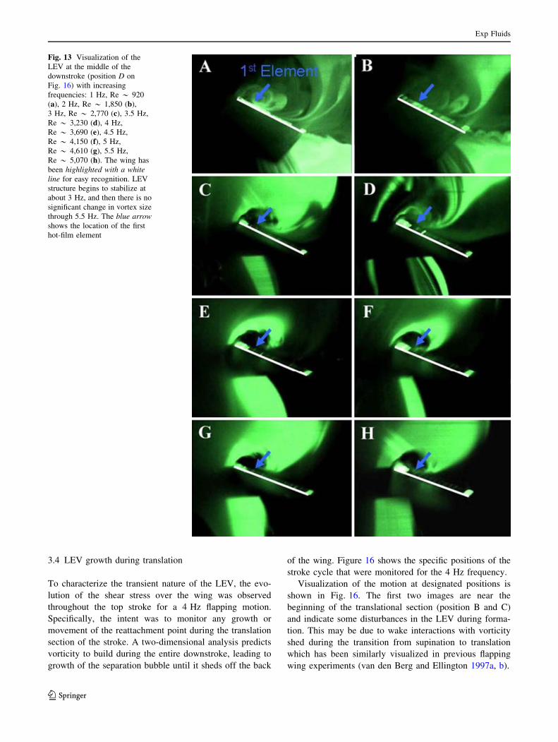
The first two images of 1 and 2 Hz indicate that the LEV

does not stabilize at low frequencies. When LEV stability

is not attained, the vortices caused by leading edge sepa-

ration are shed back along the chord. The periodic

0 0.05 0.1 0.15 0.2 0.250

0.5

1

1.5

2

2.5

Rel

ativ

e S

hea

r (

τ / τ

0 )

Time (s)

A B C D E F 123456

-80 -60 -40 -20 0 20 40 60 80-20

0

20

Horizontal Angle (°°)Ver

tica

l An

gle

(°)

A

B

CD

E

F

Fig. 11 Top Relative shear stress for hot-film sensors 1–6 vs. time

over a full flapping cycle at a flapping frequency of 4 Hz. BottomShows marked points during the flapping cycle. Points A and Drepresent the beginning and ending of the top stroke, respectively

Exp Fluids

123

shedding of the leading edge vorticity results in an aver-

aged chaotic region above the entire wing. At 3 Hz, vor-

ticity begins to stabilize at the leading edge, but the

structure appears disrupted along the outside of the vortex

core. This instability indicates that the LEV is not com-

pletely stable and still likely to shed or be disrupted later in

the stroke period. However, at 3.5 Hz, a clear LEV struc-

ture is present with far less instability around the vortex

core. As frequency increases, this instability is diminished

and a consistent leading edge structure appears and remains

stable on the leading edge.

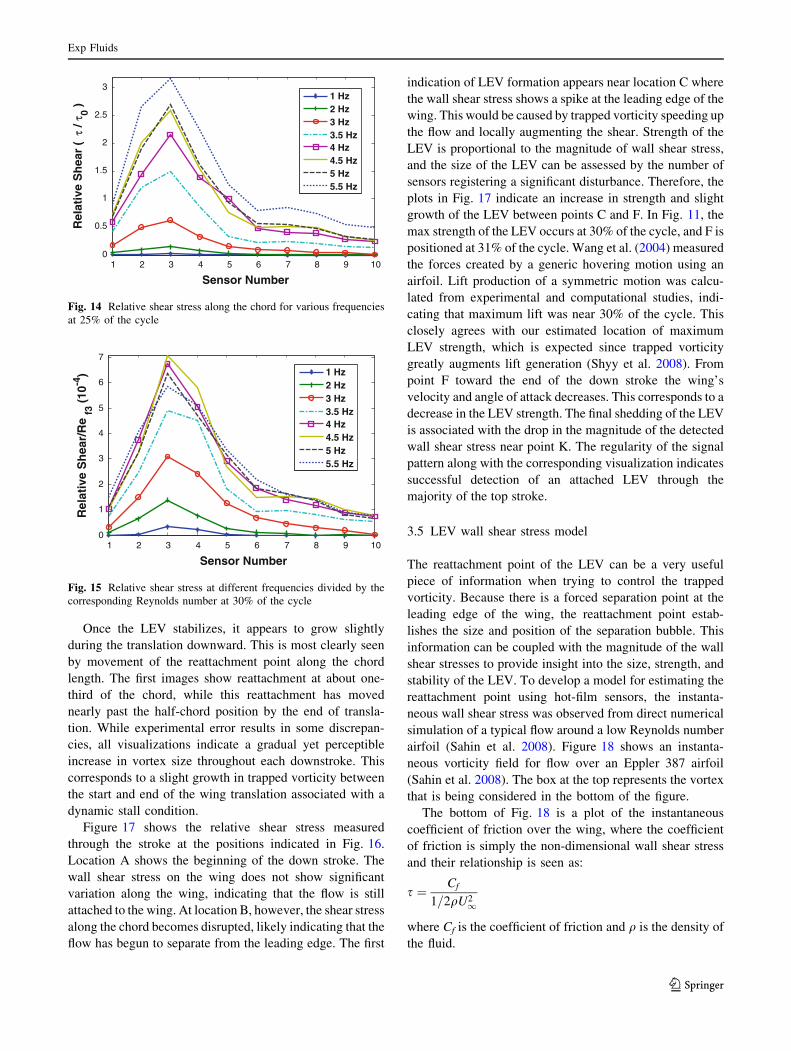
Figure 14 shows resulting sensor signals at 25% of the

cycle for each frequency. As the frequency of the motion

increases, the peaks in the shear stress increase in magni-

tude but remain near the same relative position. The

increase in signal strength suggests that the vortex strength

increase with higher flapping frequency, which is to be

expected. The peaks of the signals are constant within the

spatial resolution of the sensors, so the vortex location

stays within ±0.063 chord lengths for these frequencies.

There is a large jump in vortex strength from 2 to 3 Hz and

an even larger jump to 3.5 Hz, which agrees with the

visualization that there is a minimum frequency before a

stable vortex forms. However, if there is a critical fre-

quency where vorticity builds too rapidly to stabilize, we

did not reach it in our experimentation up to 6 Hz.

Interestingly, while there is an evolution of LEV sta-

bility with increasing frequency, the size of the LEV does

not appear to change noticeably between the frequencies

tested. Since the wing path is unchanged, a two-dimen-

sional analysis would hypothesize increasing vorticity and

augmented LEV size at higher wing speeds. However, the

uniform size seems to support the existence of a mecha-

nism that removes vorticity from the LEV, thus stabilizing

a dynamic stall condition and maintaining the LEV size.

To further study the frequency influence on the LEV,

the relationship of relative shear stress and the Reynolds

number is examined. Equation 1 is used to calculate the

Reynolds number. Because the relative shear stress and

the Reynolds number both increase with frequency, the

relative shear distribution divided by the corresponding

Reynolds number may provide insight into the charac-

teristics of LEV production with regard to flapping fre-

quency. Figure 15 shows a plot of this normalized shear

stress at 30% of the stroke cycle, which corresponds to

the point where maximum vortex strength occurs for

frequencies 1–5 Hz.

Interestingly, the maximum normalized shear increases

with frequency until it peaks at 4.5 Hz, at which point the

trend collapses with decreased normalized shear for 5 and

5.5 Hz. It is difficult to confidently characterize this

behavior of the LEV without higher resolution shear

measurements or more complex flow visualization. How-

ever, this trend should be investigated further and may

provide insight into the interaction and effectiveness of

certain flapping flight parameters.

2 4 6 8 100

0.5

1

1.5

2

2.5

Relative Shear at 4.5 Hz, at 25% of the Cycle

Sensor Number

Rel

ativ

e S

hea

r (

τ /

τ 0 )

2 4 6 8 100

0.5

1

1.5

2

2.5

Relative Shear at 3.5 Hz,at 25% of the Cycle

Sensor Number

Rel

ativ

e S

hea

r (

τ /

τ 0 )

Fig. 12 Sensor output and

smoke visualization with signal

overlay at the middle of the top

stroke at 3.5 Hz (top) and at

4.5 Hz (bottom)

Exp Fluids

123

3.4 LEV growth during translation

To characterize the transient nature of the LEV, the evo-

lution of the shear stress over the wing was observed

throughout the top stroke for a 4 Hz flapping motion.

Specifically, the intent was to monitor any growth or

movement of the reattachment point during the translation

section of the stroke. A two-dimensional analysis predicts

vorticity to build during the entire downstroke, leading to

growth of the separation bubble until it sheds off the back

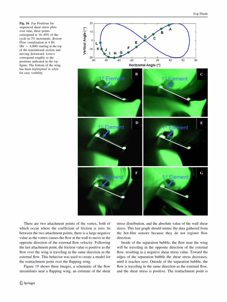
of the wing. Figure 16 shows the specific positions of the

stroke cycle that were monitored for the 4 Hz frequency.

Visualization of the motion at designated positions is

shown in Fig. 16. The first two images are near the

beginning of the translational section (position B and C)

and indicate some disturbances in the LEV during forma-

tion. This may be due to wake interactions with vorticity

shed during the transition from supination to translation

which has been similarly visualized in previous flapping

wing experiments (van den Berg and Ellington 1997a, b).

Fig. 13 Visualization of the

LEV at the middle of the

downstroke (position D on

Fig. 16) with increasing

frequencies: 1 Hz, Re * 920

(a), 2 Hz, Re * 1,850 (b),

3 Hz, Re * 2,770 (c), 3.5 Hz,

Re * 3,230 (d), 4 Hz,

Re * 3,690 (e), 4.5 Hz,

Re * 4,150 (f), 5 Hz,

Re * 4,610 (g), 5.5 Hz,

Re * 5,070 (h). The wing has

been highlighted with a whiteline for easy recognition. LEV

structure begins to stabilize at

about 3 Hz, and then there is no

significant change in vortex size

through 5.5 Hz. The blue arrowshows the location of the first

hot-film element

Exp Fluids

123

Once the LEV stabilizes, it appears to grow slightly

during the translation downward. This is most clearly seen

by movement of the reattachment point along the chord

length. The first images show reattachment at about one-

third of the chord, while this reattachment has moved

nearly past the half-chord position by the end of transla-

tion. While experimental error results in some discrepan-

cies, all visualizations indicate a gradual yet perceptible

increase in vortex size throughout each downstroke. This

corresponds to a slight growth in trapped vorticity between

the start and end of the wing translation associated with a

dynamic stall condition.

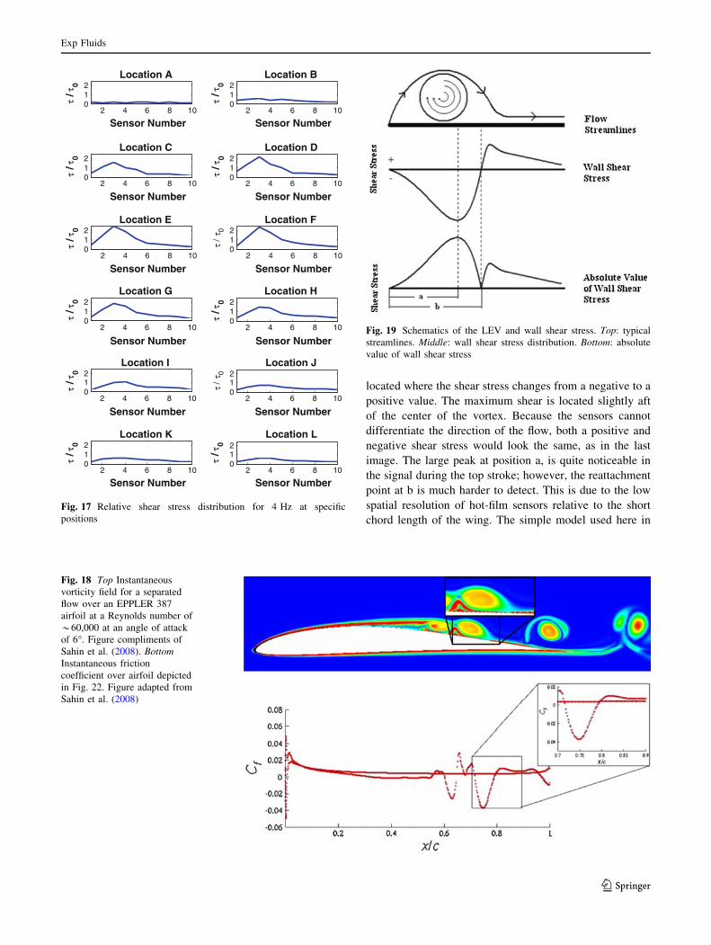
Figure 17 shows the relative shear stress measured

through the stroke at the positions indicated in Fig. 16.

Location A shows the beginning of the down stroke. The

wall shear stress on the wing does not show significant

variation along the wing, indicating that the flow is still

attached to the wing. At location B, however, the shear stress

along the chord becomes disrupted, likely indicating that the

flow has begun to separate from the leading edge. The first

indication of LEV formation appears near location C where

the wall shear stress shows a spike at the leading edge of the

wing. This would be caused by trapped vorticity speeding up

the flow and locally augmenting the shear. Strength of the

LEV is proportional to the magnitude of wall shear stress,

and the size of the LEV can be assessed by the number of

sensors registering a significant disturbance. Therefore, the

plots in Fig. 17 indicate an increase in strength and slight

growth of the LEV between points C and F. In Fig. 11, the

max strength of the LEV occurs at 30% of the cycle, and F is

positioned at 31% of the cycle. Wang et al. (2004) measured

the forces created by a generic hovering motion using an

airfoil. Lift production of a symmetric motion was calcu-

lated from experimental and computational studies, indi-

cating that maximum lift was near 30% of the cycle. This

closely agrees with our estimated location of maximum

LEV strength, which is expected since trapped vorticity

greatly augments lift generation (Shyy et al. 2008). From

point F toward the end of the down stroke the wing’s

velocity and angle of attack decreases. This corresponds to a

decrease in the LEV strength. The final shedding of the LEV

is associated with the drop in the magnitude of the detected

wall shear stress near point K. The regularity of the signal

pattern along with the corresponding visualization indicates

successful detection of an attached LEV through the

majority of the top stroke.

3.5 LEV wall shear stress model

The reattachment point of the LEV can be a very useful

piece of information when trying to control the trapped

vorticity. Because there is a forced separation point at the

leading edge of the wing, the reattachment point estab-

lishes the size and position of the separation bubble. This

information can be coupled with the magnitude of the wall

shear stresses to provide insight into the size, strength, and

stability of the LEV. To develop a model for estimating the

reattachment point using hot-film sensors, the instanta-

neous wall shear stress was observed from direct numerical

simulation of a typical flow around a low Reynolds number

airfoil (Sahin et al. 2008). Figure 18 shows an instanta-

neous vorticity field for flow over an Eppler 387 airfoil

(Sahin et al. 2008). The box at the top represents the vortex

that is being considered in the bottom of the figure.

The bottom of Fig. 18 is a plot of the instantaneous

coefficient of friction over the wing, where the coefficient

of friction is simply the non-dimensional wall shear stress

and their relationship is seen as:

s ¼ Cf

1=2qU21

where Cf is the coefficient of friction and q is the density of

the fluid.

1 2 3 4 5 6 7 8 9 100

0.5

1

1.5

2

2.5

3

Sensor Number

Rel

ativ

e S

hea

r (

τ / τ

0 )

1 Hz2 Hz3 Hz3.5 Hz4 Hz4.5 Hz5 Hz5.5 Hz

Fig. 14 Relative shear stress along the chord for various frequencies

at 25% of the cycle

1 2 3 4 5 6 7 8 9 100

1

2

3

4

5

6

7

Sensor Number

Rel

ativ

e S

hea

r/R

ef3

(10

-4) 1 Hz

2 Hz3 Hz3.5 Hz4 Hz4.5 Hz5 Hz5.5 Hz

Fig. 15 Relative shear stress at different frequencies divided by the

corresponding Reynolds number at 30% of the cycle

Exp Fluids

123

There are two attachment points of the vortex, both of

which occur where the coefficient of friction is zero. In

between the two attachment points, there is a large negative

value as the vortex causes the flow at the wall to move in the

opposite direction of the external flow velocity. Following

the last attachment point, the friction value is positive as the

flow over the wing is traveling in the same direction as the

external flow. This behavior was used to create a model for

the reattachment point over the flapping wing.

Figure 19 shows three images, a schematic of the flow

streamlines near a flapping wing, an estimate of the shear

stress distribution, and the absolute value of the wall shear

stress. This last graph should mimic the data gathered from

the hot-film sensors because they do not register flow

direction.

Inside of the separation bubble, the flow near the wing

will be traveling in the opposite direction of the external

flow, resulting in a negative shear stress value. Toward the

edges of the separation bubble the shear stress decreases,

until it reaches zero. Outside of the separation bubble, the

flow is traveling in the same direction as the external flow,

and the shear stress is positive. The reattachment point is

Fig. 16 Top Positions for

sequenced shear stress plots

over time, these points

correspond to 16–49% of the

cycle in 3% increments. BottomFlow visualization at 4 Hz

(Re * 4,000) starting at the top

of the translational section and

moving downward. Letterscorrespond roughly to the

positions indicated in the topfigure. The bottom of the wing

has been highlighted in whitefor easy visibility

Exp Fluids

123

located where the shear stress changes from a negative to a

positive value. The maximum shear is located slightly aft

of the center of the vortex. Because the sensors cannot

differentiate the direction of the flow, both a positive and

negative shear stress would look the same, as in the last

image. The large peak at position a, is quite noticeable in

the signal during the top stroke; however, the reattachment

point at b is much harder to detect. This is due to the low

spatial resolution of hot-film sensors relative to the short

chord length of the wing. The simple model used here in

2 4 6 8 10012

Location A

Sensor Number

τ / τ

0

2 4 6 8 10012

Location B

Sensor Number

τ / τ

0

2 4 6 8 10012

Location C

Sensor Number

τ / τ

0

2 4 6 8 10012

Location D

Sensor Number

τ / τ

0

2 4 6 8 10012

Location E

Sensor Number

τ / τ

0

2 4 6 8 10012

Location F

Sensor Number

τ /

τ 0

2 4 6 8 10012

Location G

Sensor Number

τ / τ

0

2 4 6 8 10012

Location H

Sensor Number

τ / τ

0

2 4 6 8 10012

Location I

Sensor Number

τ / τ

0

2 4 6 8 10012

Location J

Sensor Number

τ /

τ 0

2 4 6 8 10012

Location K

Sensor Number

τ / τ

0

2 4 6 8 10012

Location L

Sensor Number

τ / τ

0

Fig. 17 Relative shear stress distribution for 4 Hz at specific

positions

Fig. 18 Top Instantaneous

vorticity field for a separated

flow over an EPPLER 387

airfoil at a Reynolds number of

*60,000 at an angle of attack

of 6�. Figure compliments of

Sahin et al. (2008). BottomInstantaneous friction

coefficient over airfoil depicted

in Fig. 22. Figure adapted from

Sahin et al. (2008)

Fig. 19 Schematics of the LEV and wall shear stress. Top: typical

streamlines. Middle: wall shear stress distribution. Bottom: absolute

value of wall shear stress

Exp Fluids

123

order to determine the reattachment point assumes that the

ratio of a and b is constant regardless of the vortex size.

This ratio was determined experimentally by analyzing

flow visualizations with a visible reattachment point and

comparing them with the measured shear distribution. The

peak point in the signal was determined and then fit to a

parabolic curve with the adjacent sensor reading. The

maximum value of the parabolic curve is then taken as

position a. Comparing with the reattachment position in the

visualization, the ratio b/a was calculated to be 1.22.

Because this type of analysis is particularly sensitive to the

signal and noise level, a linear regression was fit to each

signal to show the trend of reattachment behavior. The

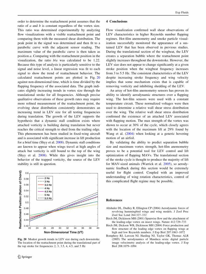
calculated reattachment points are plotted in Fig. 20

against non-dimensional time, which is time divided by the

flapping frequency of the associated data. The graph indi-

cates slightly increasing trends in vortex size through the

translational stroke for all frequencies. Although precise

qualitative observations of these growth rates may require

more refined measurement of the reattachment point, the

evolving shear distribution consistently demonstrates an

increasing trend in LEV size for all testing frequencies

during translation. The growth of the LEV supports the

hypothesis that a dynamic stall condition exists where

attached vorticity is building during translation but never

reaches the critical strength to shed from the trailing edge.

This phenomenon has been studied in fixed-wing aircraft

and is associated with significant increase in lift production

for a brief time (Shyy et al. 2008). Dynamic stall conditions

are known to appear when wings travel at high angles of

attack but vorticity is still bound to the top of the wing

(Shyy et al. 2008). While this gives insight into the

behavior of the trapped vorticity, the source of the LEV

stability is still in question.

4 Conclusions

Flow visualization confirmed wall shear observations of

LEV characteristics in higher Reynolds number flapping

regimes. Hot-film anemometry and smoke particle visual-

ization successfully monitored the appearance of a sus-

tained LEV that has been observed in previous studies.

During the translational section of the wingbeat, the LEV

creates a separation bubble where the reattachment point

slightly increases throughout the downstroke. However, the

LEV size does not appear to change significantly at a given

stroke position when the wingbeat frequency increases

from 3 to 5.5 Hz. The consistent characteristics of the LEV

despite increasing stroke frequency and wing velocity

implies that some mechanism exists that is capable of

removing vorticity and inhibiting shedding of the LEV.

An array of hot-film anemometry sensors has proven its

ability to identify aerodynamic structures over a flapping

wing. The hot-film sensors were used with a constant

temperature circuit. These normalized voltages were then

used to determine a relative wall shear stress distribution

over the wing. The relative wall shear stress distribution

confirmed the existence of an attached LEV associated

with flapping motion. The max strength of the vortex was

shown to occur at 30% of the cycle, which closely agrees

with the location of the maximum lift at 29% found by

Wang et al. (2004) when looking at a generic hovering

motion of an airfoil.

By validating the ability to predict separation bubble

size and maximum vortex strength, hot-film anemometry

proves to be a potential tool for LEV control and lift

optimization of flapping MAVs. The translational section

of the stroke cycle is thought to produce the majority of lift

for MAV-sized animals (Warrick et al. 2005), so aerody-

namic feedback during this section would be extremely

useful for flight control. Coupled with an improved

understanding of wing rotation characteristics, control of

this complicated flight regime may be possible.

References

Altshuler DL, Dudley R, Ellington CP (2004) Aerodynamic forces of

revolving hummingbird wings and wing models. J Zool Proc

Zool Soc Lond 264:327–332

Birch JM, Dickinson MH (2001) Spanwise flow and the attachment of

the leading-edge vortex on insect wings. Nature 412:729–733

Birch JM, Dickson WB, Dickinson MH (2004) Force production and

flow structure of the leading edge vortex on flapping wings at

high and low Reynolds numbers. J Exp Biol 207:1063–1072

Bomphrey RJ, Lawson NJ, Harding NJ, Taylor GK, Thomas ALR

(2005) The aerodynamics of Manduca sexta: digital particle

image velocimetry analysis of the leading-edge vortex. J Exp

Biol 208:1079–1094

22 24 26 28 30 32 34 36 38 400.42

0.44

0.46

0.48

0.5

0.52

0.54

0.56

0.58

0.6

Non-Dimensional Time (t/T)

Rea

ttac

hm

ent

Po

siti

on

(R

atio

n o

f C

ho

rd)

2 Hz3 Hz3.5 Hz4 Hz4.5 Hz5 Hz5.5 Hz

Fig. 20 Modest growth trends in LEV size during each downstroke.

The location of the reattachment point during the translational part of

the top stroke for frequencies 2, 3, 3.5, 4, 4.5, and 5 Hz

Exp Fluids

123

Dickinson MH, Gotz KG (1993) Unsteady aerodynamic performance

of model wings at low Reynolds numbers. J Exp Biol 174:45–64

Dickinson MH, Lehmann FO, Sane SP (1999) Wing rotation and the

aerodynamic basis of insect flight. Science 284:1954–1960

Maxworthy T (1979) Experiments on the Weis-Fogh mechanism of

lift generation by insects in hovering flight. Part 1. Dynamics of

the ‘fling’. J Fluid Mech 93:47–63

Saffman PG, Sheffield JS (1977) Flow over a wing with an attached

free vortex. Stud Appl Math 57:107–117

Saharon D, Luttges MW (1988) Visualization of unsteady separated

flow produces by mechanically driven dragonfly wing kinemat-

ics model. AIAA J 88-0569:1–23

Sahin M, Hall J, Mohseni K (2008) Direct numerical simulation of

separated low-reynolds number flows around an Eppler 387

Airfoil. 46th AIAA Aerospace Sciences Meeting and Exhibit.

Reno, NV, 7–10 Jan 2008

Sane SP (2003) The aerodynamics of insect flight. J Exp Biol

206:4149–4208

Sane SP, Dickinson MH (2001) The control of flight force by a flapping

wing: lift and drag production. J Exp Biol 204:2607–2626

Shyy W, Lian Y, Tang J, Viieru D, Liu H (2008) Aerodynamics of low

Reynolds number flyers. Cambridge University Press, New York

Srygley RB, Thomas LR (2002) Unconventional lift-generating

mechanisms in free-flying butterflies. Nature 420:660–664

Tavoularis S (2005) Measurement in fluid mechanics. Cambridge

University Press, New York

Thomas LR, Taylor GK, Srygley RB, Nudds RL, Bomphrey RJ (2004)

Dragonfly flight: free-flight and tethered flow visualizations

reveal a diverse array of unsteady lift-generating mechanisms,

controlled primarily via angle of attack. J Exp Biol 207:4299–

4323

Tobalske BW, Warrick DR, Clark CJ, Powers DR, Hedrick TL,

Hyder GA, Biewener AA (2007) Three-dimensional kinematics

of hummingbird flight. J Exp Biol 210:2368–2382

Usherwood JR, Ellington CP (2002) The aerodynamics of revolving

wings (I. Model hawkmoth wings). J Exp Biol 205:1547–1564

van den Berg C, Ellington CP (1997a) The vortex wake of a

‘hovering’ model hawkmoth. Phil Trans R Soc Lond B 352:317–

328

van den Berg C, Ellington CP (1997b) The three-dimensional leading-

edge vortex of a ‘hovering’ model hawkmoth. Phil Trans R Soc

Lond B 352:329–340

Vanier B (2008) Detection of aerodynamic flow structures during

hummingbird like flapping motion using hot film anemometry

tavoularix. Master’s Thesis. University of Colorado at Boulder

Wang ZJ, Birch JM, Dickinson MH (2004) Unsteady forces and flows

in a low Reynolds number hovering flight: two-dimensional

computations vs. robotic wing experiments. J Exp Biol 207:449–

460

Warrick DR, Tobalske BW, Powers DR (2005) Aerodynamics of the

hovering hummingbird. Nature 435:1094–1097

Weis-Fogh T (1973) Quick estimates of flight fitness in hovering

animals, including novel mechanisms for lift production. J Exp

Biol 59:169–230

Exp Fluids

123