Embed Size (px)
Citation preview

IOP PUBLISHING JOURNAL OF PHYSICS: CONDENSED MATTER
J. Phys.: Condens. Matter 24 (2012) 213202 (23pp) doi:10.1088/0953-8984/24/21/213202
TOPICAL REVIEW
First-principle calculations of the Berrycurvature of Bloch states for charge andspin transport of electrons
M Gradhand1,2, D V Fedorov1,3, F Pientka3,4, P Zahn3,5, I Mertig1,3 and
B L Gyorffy2
1 Max Planck Institute of Microstructure Physics, Weinberg 2, 06120 Halle, Germany2 H H Wills Physics Laboratory, University of Bristol, Bristol BS8 1TH, UK3 Institute of Physics, Martin Luther University Halle-Wittenberg, 06099 Halle, Germany4 Dahlem Center for Complex Quantum Systems and Fachbereich Physik, Freie Universitat Berlin,
14195 Berlin, Germany5 Institute of Ion Beam Physics and Materials Research, Helmholtz-Zentrum Dresden-Rossendorf e.V.,
PO Box 510119, 01314 Dresden, Germany
E-mail: [email protected]
Received 15 February 2012, in final form 3 April 2012
Published 11 May 2012
Online at stacks.iop.org/JPhysCM/24/213202
Abstract
Recent progress in wave packet dynamics based on the insight of Berry pertaining to adiabatic
evolution of quantum systems has led to the need for a new property of a Bloch state, the
Berry curvature, to be calculated from first principles. We report here on the response to this
challenge by the ab initio community during the past decade. First we give a tutorial
introduction of the conceptual developments we mentioned above. Then we describe four
methodologies which have been developed for first-principle calculations of the Berry
curvature. Finally, to illustrate the significance of the new developments, we report some
results of calculations of interesting physical properties such as the anomalous and spin Hall
conductivity as well as the anomalous Nernst conductivity and discuss the influence of the
Berry curvature on the de Haas–van Alphen oscillation.
(Some figures may appear in colour only in the online journal)
Contents
1. Introduction: semiclassical electronic transport in
solids, wave packet dynamics, and the Berry
curvature 2
1.1. New features of the Boltzmann equation 2
1.2. Berry phase, connection and curvature of Bloch
electrons 3
1.3. Abelian and non-Abelian curvatures 4
1.4. Symmetry, topology, codimension and the
Dirac monopole 5
1.5. The spin polarization gauge 6
2. First-principle calculations of the Berry curvature forBloch electrons 8
2.1. KKR method 8
2.2. Tight-binding model 10
2.3. Wannier interpolation scheme 13
2.4. Kubo formula 15
3. Intrinsic contribution to the charge and spinconductivity in metals 17
4. De Haas–van Alphen oscillation and the Berry phases 20
5. Conclusion 21
Acknowledgments 22
References 22
10953-8984/12/213202+23$33.00 c© 2012 IOP Publishing Ltd Printed in the UK & the USA

J. Phys.: Condens. Matter 24 (2012) 213202 Topical Review
1. Introduction: semiclassical electronic transport insolids, wave packet dynamics, and the Berrycurvature
Some recent, remarkable advances in the semiclassical
description of charge and spin transport by electrons in
solids motivate a revival of interest in a detailed k-point by
k-point study of their band structure. A good summary of
the conceptual developments and the experiments they have
stimulated has been given by Di Xiao et al [1]. Here we
wish to review only the role and prospects of first-principle
electronic structure calculations in this rapidly moving field.
1.1. New features of the Boltzmann equation
Classically, particle transport is considered to take place in
phase space, whose points are labeled by the position vector
r and the momentum p, and is described by the distribution
function f (r, p, t), which satisfies the Boltzmann equation.
Electrons in solids fit into this framework if we view the
particles as wave packets constructed from the Bloch waves,
9nk (r) = eik·run(r, k), eigenfunctions of the unperturbed
crystal Hamiltonian H0 with band index n and the dispersion
relation Enk. If such a wave packet is strongly centered at
kc in the Brillouin zone, it predominantly includes Bloch
states with quantum numbers k close to kc and the particle
can be said to have a momentum hkc. Then, if we call its
spatial center rc its position, the transport of electrons can
be described by an ensemble of such quasiparticles. One of
them is described by the distribution function fn(rnc, kn
c, t).
For simplicity, the band index n is dropped in the following
for f , rc, and kc. As f (rc, kc, t) evolves in phase space, the
usual form of the Boltzmann equation, which preserves the
total probability, is given by
∂tf + rc ·∇rc f + kc ·∇kc f =(
δf
δt
)
scatt
. (1)
Here the first term on the left hand side is the derivative with
respect to the explicit time dependence of f , the next two
terms account for the time dependence of rc and kc, and the
term on the right-hand side describes the scattering of electron
states, by defects and other perturbations, in and out of the
considered phase space volume centered at rc and kc. The
time evolution of rc(t) and kc(t) is given by semiclassical
equations of motion, which in the presence of external electric
E and magnetic B fields take conventionally the following
form:
rc = 1
h
∂Enk
∂k
∣∣∣∣k=kc
= vn(kc), (2)
hkc = −eE − erc × B. (3)
Here, the group velocity vn(kc) involves the unperturbed
band structure. In the presence of a constant electric E =(Ex, 0, 0) and magnetic B = (0, 0, Bz) field, the solution of the
above equations yields the Hall resistivity ρxy ∝ Bz. However,
for a ferromagnet with magnetization M = (0, 0, Mz)
the above theory cannot account for the experimentally
observed (additional) anomalous contribution ρxy ∝ Mz. For
a necessary correction of the theory, one needs to construct a
wave packet [2]
Wkc,rc(r, t) =∑
k
ak(kc, t)9nk(r), (4)
carefully taking into account the phase of the weighting
function ak(kc, t). Requiring the wave packet to be
centered at rc = 〈Wkc,rc |r|Wkc,rc〉 and considering zero
order in the magnetic field only, it follows that ak(kc, t) =|ak(kc, t)|ei(k−kc)·An(kc)−ik·rc [2], where
An(kc) = i
∫
u.c.
d3r u∗n(r, kc)∇kun(r, kc) (5)
is the Berry connection, as will be discussed in detail in
section 1.2. Note that the integral is restricted to only one unit
cell (uc). Now, using the wave packet of equation (4), one can
construct the Lagrangian
L(t) = 〈W| ih∂t − H |W〉 (6)
and minimize the action functional S[rc(t), kc(t)] =∫ t
dt′L(t′)with respect to arbitrary variations in rc(t) and kc(t).
This maneuver replaces the quantum mechanical expectation
values with respect to Wkc,rc(r, t) by the classical equations
of motion for rc(t) and kc(t). From the Euler–Lagrange
equations
d
dt
∂L
∂kc
− ∂L
∂kc= 0 and
d
dt
∂L
∂ rc− ∂L
∂rc= 0, (7)
one gets
rc = 1
h
∂Enk
∂k|k=kc − kc × Ωn (kc) , (8)
hkc = −eE − erc × B. (9)
Here Ωn(kc) is the so-called Berry curvature, defined as
Ωn(kc) = ∇k × An(k)|k=kc , (10)
the main subject of this review. For simplicity, several further
terms in equations (8) and (9) were neglected. These are fully
discussed in [1, 2]. For the purpose of this review the above
form is sufficient to highlight the occurrence of the Berry
curvature in the equations of motion.
In comparison to equation (2), the new equation of
motion for rc(t) given by equation (8) has an additional term
proportional to the electric field called the anomalous velocity
van(kc) = e
hE × Ωn (kc) . (11)
The presence of this velocity provides the anomalous
contribution to the Hall current jHy = jH,↑y + j
H,↓y , where the
spin-resolved currents may be written as
jH,↑y = −e
∫
BZ
d3kc
(2π)3r
yc↑(kc)f↑(kc) = σ↑
yx(Mz)Ex. (12)
jH,↓y = −e
∫
BZ
d3kc
(2π)3r
yc↓(kc)f↓(kc) = σ↓
yx(Mz)Ex. (13)
2

J. Phys.: Condens. Matter 24 (2012) 213202 Topical Review
Figure 1. (a) The anomalous Hall effect and (b) the spin Hall effect.
In this notation f↑(kc) and f↓(kc) are the spin-resolved
distribution functions which are solutions of equation (1).
Here rc and t are dropped due to homogeneous and
steady state conditions. In the limit of no scattering they
reduce to the equilibrium distribution functions and only the
intrinsic mechanism, governed by the anomalous velocity of
equation (11), contributes to the Hall component. In general,
jH,↑y and j
H,↓y have opposite signs because of rc↓(kc) and
rc↑(kc). However, the resulting charge current is nonvanishing
(see figure 1(a)) due to the fact that the numbers of spin-up
and spin-down electrons differ in ferromagnets with a finite
magnetization M 6= 0. In contrast to the anomalous Hall effect
(AHE) in ferromagnets, the absence of the magnetization
in normal metals leads to the presence of time inversion
symmetry and, as a consequence, jH,↑y = −j
H,↓y . This implies a
vanishing charge current, i.e. Hall voltage, but the existence of
a pure spin current as depicted in figure 1(b), which is known
as the spin Hall effect (SHE).
1.2. Berry phase, connection and curvature of Blochelectrons
Here we introduce briefly the concept of such relatively novel
quantities as the Berry phase, connection, and curvature which
arise in the case of an adiabatic evolution of a system.
1.2.1. Adiabatic evolution and the Berry phase. Let us
consider an eigenvalue problem of the following form:
H(r, λ1, λ2, λ3)8n(r; λ1, λ2, λ3)
= En(λ1, λ2, λ3)8n(r; λ1, λ2, λ3), (14)
where H is a differential operator, 8n and En are the nth
eigenfunction and eigenvalue, respectively, the vector r is
a variable, and λ1, λ2, λ3 are parameters. A mathematical
problem of general interest is the way such eigenfunctions
change if the set λ = (λ1, λ2, λ3) changes slowly with
time. If it is assumed that the process is adiabatic, that
is to say there is no transition from one to another state,
then for a long time it was argued that a state 8n(r, λ, t)
evolves in time as 8n(r, λ, t) = 8n(r, λ) exp(− ih
∫ t
0 dt′En
(λ1(t′), λ2(t
′), λ3(t′)) + iγn(t)), where the phase γn(t) is
meaningless as it can be gauged away. In 1984 Berry [3]
discovered that, while this is true for an arbitrary open path
in the parameter space, for a path that returns to the starting
values λ1(0), λ2(0), and λ3(0) the accumulated phase is
gauge invariant and is therefore a meaningful and measurable
Figure 2. A closed path in the parameter space.
quantity. In particular, he showed that for a closed path,
labeled C in figure 2, the phase γn, called the Berry phase
today, can be described by a line integral as
γn =∮
C
dλ · An(λ), (15)
where the connection An(λ) is given by
An(λ) = i
∫d3r 8∗
n(r, λ)∇λ8n(r, λ). (16)
The surprise is that, although the connection is not gauge
invariant, γn and even more interestingly the curvature
Ωn(λ) = ∇λ × An(λ) (17)
are. As will be shown presently, these ideas are directly
relevant for the dynamics of wave packets in the transport
theory discussed above.
1.2.2. Berry connection and curvature for Bloch states.
Somewhat surprisingly, the above discussion has a number
of interesting things to say about the wave packets in the
semiclassical approach for spin and charge transport of
electrons in crystals. Its relevance becomes evident if we take
the Schrodinger equation for the Bloch state
(− h2
2m∇
2r + V(r)
)9nk(r) = Enk9nk(r) (18)
3

J. Phys.: Condens. Matter 24 (2012) 213202 Topical Review
and rewrite it for the periodic part of the Bloch function
(− h2
2m(∇r + ik)2 + V(r)
)un(r, k) = Enkun(r, k). (19)
The point is that the differential equation for 9nk(r), a
simultaneous eigenfunction of the translation operator and the
Hamiltonian, does not depend on the wave vector, since k only
labels the eigenvalues of the translation operator. However, in
equation (19) k appears as a parameter and hence the above
discussion of the Berry phase, the corresponding connection,
and curvature applies directly to the periodic part of the
wave function un(r, k). In short, for each band n there is a
connection associated with every k given by
An(k) = i
∫
uc
d3r u∗n(r, k)∇kun(r, k). (20)
Furthermore, the curvature
Ωn(k) = ∇k × An(k)
= i
∫
uc
d3r∇ku∗n(r, k) × ∇kun(r, k) (21)
is the quantity that appears in the semiclassical equation
of motion for the wave packet in equation (8). Thus,
the curvature and the corresponding anomalous velocity in
equations (11) associated with the band n are properties of
un(r, k). To emphasize this point, we note that the Bloch
functions 9nk(r) are orthogonal to each other
〈9nk|9n′k′〉 =∫
crystal
d3r 9∗nk(r)9n′k′(r) = δk,k′δn,n′ , (22)
and hence k is not a parameter. In contrast, un(r, k) is
orthogonal to un′(r, k) but not necessarily to un(r, k′), as this
is an eigenfunction of a different Hamiltonian.
The observation that the above connection and curvature
are properties of the periodic part of the Bloch function
prompts a further comment. Note that for vanishing periodic
potential the Bloch functions would reduce to plane waves.
Constructing the wave packet from plane waves means
un(r, k) = 1. Evidently, this means that Ωn(k) and An(k)
vanish, and this fact is consistent with the general notion that
the connection and the curvature arise from including only
one or in any case a finite number of bands in constructing
the wave packet. The point is that the neglected bands are the
‘outside world’ referred to in the original article of Berry [3].
In contrast, the expansion in terms of plane waves does not
neglect any bands since there is just one band. Thus, the
physical origin of the connection and the curvature is due to
the periodic crystal potential breaking up the full spectrum of
the parabolic free particle dispersion relation into bands. They
are usually separated by gaps, and we select states only from
a limited number of such bands to represent the wave packet.
1.3. Abelian and non-Abelian curvatures
So far we have introduced the Berry connection and
curvature for a nondegenerate band. In the case of degenerate
bands the conventional adiabatic theorem fails. In the
semiclassical framework a correct treatment incorporates a
wave packet constructed from the degenerate bands [4, 5].
As a consequence, the Berry curvature must be extended to
a tensor definition in analogy to non-Abelian gauge theories.
This extension is originally due to Wilczek and Zee [6].
Let us consider the eigenspace |ui(k)〉 : i ∈ 6 of some
N-fold degenerate eigenvalue. For Bloch states the elements
of the non-Abelian Berry connection ¯A(k) read
Aij(k) = i〈ui(k)|∇kuj(k)〉 i, j ∈ 6, (23)
where 6 = 1, . . . , N contains all indices of the degenerate
subspace. The definition of the curvature tensor ¯Ω(k) in a
non-Abelian gauge theory has to be extended by substituting
the curl with the covariant derivative as [5]
¯Ω(k) = ∇k × ¯A(k) − i ¯A(k) × ¯A(k),
Ωij(k) = i
⟨∂ui(k)
∂k
∣∣∣∣×∣∣∣∣∂uj(k)
∂k
⟩
+ i∑
l∈6
⟨ui(k)
∣∣∣∣∂ul(k)
∂k
⟩×⟨ul(k)
∣∣∣∣∂uj(k)
∂k
⟩.
(24)
The subspace of degenerate eigenstates is subject to a U(N)
gauge freedom and observables should be invariant with
respect to a gauge transformation of the basis set∑
i
Uji(k) |ui(k)〉 : i ∈ 6
with ¯U(k) ∈ U(N).
(25)
Consequently, the Berry connection and curvature are
transformed according to
¯A′(k) = ¯U
†(k) ¯A(k) ¯U(k) + i ¯U
†(k)∇k
¯U(k), (26)
¯Ω
′(k) = ¯U
†(k) ¯
Ω(k) ¯U(k). (27)
The curvature is now a covariant tensor and thus not directly
observable. However, there are gauge invariant quantities that
may be derived from it. From gauge theories it is known that
the connection and the curvature must lie in the tangent space
of the gauge group U(N), i.e., the Lie algebra u(N). The above
definition of the Lie algebra differs by an unimportant factor
of i from the mathematical convention.
The most prominent example of a non-Abelian Berry
curvature appears in materials with time-reversal (T) and
inversion (I) symmetry. For each k point there exist two
orthogonal states |9n↑k〉 and |9n↓k〉 = TI|9n↑k〉 with the
same energy, the Kramers doublet. In general, a choice for
|9n↑k〉 determines the second basis state |9n↓k〉 only up
to a phase. However, the symmetry transformation fixes the
phase relationship between the two basis states. This reduces
the gauge freedom to SU(2) and, consequently, the Berry
connection will be an su(2) matrix, which means the trace
of the 2 × 2 matrix vanishes. This is verified easily
〈un↓(k)|∇kun↓(k)〉 = 〈TI un↑(k)|∇kTI un↑(k)〉= 〈TI un↑(k)|TI ∇kun↑(k)〉= −〈un↑(k)|∇kun↑(k)〉. (28)
4

J. Phys.: Condens. Matter 24 (2012) 213202 Topical Review
Figure 3. Left: conical intersection of energy surfaces. Right: direction of the monopole field Ω+(k).
For the Kramers doublet the Berry curvature must always be
an su(2) matrix even in the case of a u(2) connection because
a gauge transformation induces a unitary transformation
of the curvature which does not alter the trace. Indeed,
TI Ωn↑↑(k) = −Ωn↑↑(k) = Ωn↓↓(k), which proves that the
trace is equal to zero. Therefore, in contrast to the spinless
case, discussed in the next section, the Berry curvature may
be nontrivial even in nonmagnetic materials with inversion
symmetry.
Despite the Berry curvature being gauge covariant, we
may derive several observables from it. As we have seen,
the trace of the Berry curvature is gauge invariant. In
the multiband formulation of the semiclassical theory, the
expectation value of the curvature matrix with respect to the
spinor amplitudes enters the equations of motion [4, 5]. In the
context of the spin Hall effect one is interested in Tr( ¯Sα ¯
β),
where ¯Sα
is the αth component of the vector-valued su(2) spin
matrix (cf section 2.4.2).
1.4. Symmetry, topology, codimension and the Diracmonopole
It is expedient to exploit symmetries of the Hamiltonian for
the evaluation of the Berry curvature. From equations (20)
and (21) we may easily determine the behavior of Ωn(k)
under symmetry operations. In crystals with a center of
inversion, the corresponding symmetry operation leaves Enk
invariant while r, r, k, and k change sign, and hence Ωn(k) =Ωn(−k). On the other hand, when time-reversal symmetry is
present, Enk, r, and k remain unchanged while r and k are
inverted, which leads to an antisymmetric Berry curvature
Ωn(k) = −Ωn(−k). Thus, if time-reversal and inversion
symmetry are present simultaneously the Berry curvature
vanishes identically [7]. This is true for spinless particles
only. Taking into account spin, we have to acknowledge the
presence of a twofold degeneracy of all bands throughout the
Brillouin zone [8, 9], the Kramers doublet, discussed in the
previous section.
As was mentioned already in section 1.2.2, the Berry
curvature of a band arises due to the attempt of a single-band
description; e.g., in the semiclassical theory it keeps the
information about the influence of other adjacent bands.
If a band is well separated from all other bands by an
energy scale large compared to one set by the time scale of
the adiabatic evolution, the influence of the other bands is
negligible. In contrast, degeneracies of energy bands deserve
special attention, since the conventional adiabatic theorem
fails in this case. Special attention has been paid to point-like
degeneracies, where the intersection of two energy bands is
shaped like a double cone or a diabolo. These degeneracies
are called diabolical points [10]. A typical one, studied within
a tight-binding model in [11], is shown in figure 3.
In general, a Hermitian Hamiltonian H(k) with three
parameters kx, ky, kz has degeneracies (band crossings) at
points k∗. Taking k∗ as the origin and assuming that
H(k) depends linearly on the k measured from k∗, a generic
example for two bands crossing can be constructed as follows.
At k = k∗ there are two orthogonal states |a〉 and |b〉whose energies are the same, Ea = Eb = 0, which we take
to be the energy zero. In the vicinity of the point k∗ we can
express the eigenstates in terms of the two states
|un(k)〉 = can(k) |a〉 + cbn(k) |b〉 (29)
where n = +, − and the coefficients can(k) and cbn(k) are
determined by the eigenvalue problem
H(k) |un(k)〉 = Enk |un(k)〉 . (30)
Using the expansion of equation (29), little is lost in generality
by taking H(k) in the representation of the two states |a〉 and
|b〉 to be of the form [3]
H(k) =(
kz kx − iky
kx + iky −kz
), (31)
and hence the eigenvalue equation can be written as
(kz kx − iky
kx + iky −kz
)(can(k)
cbn(k)
)= Enk
(can(k)
cbn(k)
). (32)
The solution of this eigenvalue problem is
E±k = ±√
k2z + k2
x + k2y = ± |k| = ±k (33)
5

J. Phys.: Condens. Matter 24 (2012) 213202 Topical Review
and the two eigenvectors are
u+(k) ≡(
ca+(k)
cb+(k)
)=
√k + kz
2ke−i
δ+2
√k − kz
2ke+i
δ+2
(34)
δ+ = tan−1
(ky
kx
)(35)
u−(k) ≡(
ca−(k)
cb−(k)
)=
√k − kz
2ke−i
δ−2
−√
k + kz
2ke+i
δ−2
(36)
δ− = tan−1
(ky
kx
)(37)
where we used the shortcut u±(k) for the two component
eigenvectors representing the expansion coefficients of
|un(k)〉. Clearly, δ+ = δ− ≡ δ holds.
Calculating the connection
A+(k) = i u†+(k)∇ku+(k) (38)
and the curvature as
Ω+(k) = −Imu
†+(k)∇kH(k)u−(k) × u
†−(k)∇kH(k)u+(k)
(E+k − E−k)2
(39)
one finds
Ω±(k) = ∓1
2
k
k3. (40)
This is precisely the form of the magnetic field due to a
Dirac monopole, if k is replaced by the real space vector
r, with the magnetic charges ∓ 12 [3] (see figure 3, right).
Diabolical points always have this charge, while nonlinear
intersections may have higher charges [12]. In general, the
monopole charge is a topological invariant and quantized
to integer multiples of 1/2. This is a consequence of the
quantization of the Dirac monopole [13].
In more general language, the Berry curvature flux
through a closed two-dimensional manifold ∂M is the first
Chern number Cn of that manifold and thus an integer.
Since the (Abelian) curvature is defined as the curl of
the connection, it must be divergence free except for the
monopoles. We can then exploit Gauss’s theorem
Cn = 1
2π
∫
∂M
dσ Ωn(k)n(k)
= 1
2π
∫
M
d3k∇k ·Ωn = m, m ∈ N. (41)
Here n is the normal vector of the surface element. If we
assume that each monopole contributes a Chern number of
±1 the above equation implies for the Berry curvature ∇k ·
Ω(k) = 4π∑
jgjδ(k − k∗j ), where gj = ±1/2. The solution of
this differential equation yields the source term of the Berry
curvature
Ω(k) =∑
j
gj
k − k∗j
|k − k∗j |3
+ ∇k × A(k), (42)
which proves that there are monopoles with a charge
quantized to 1/2 times an integer.
The mathematical interpretation of the Berry cur-
vature in terms of the theory of fiber bundles and
Chern classes and the connection to the theory of the
quantum Hall effect, where the Chern number appears
as the Thouless–Kohmoto–Nightingale–den Nijs (TKNN)
integer [14] was first noticed by Simon [15].
However, monopoles are interesting not only in a
mathematical sense but also for actual physical quantities
such as the anomalous Hall conductivity. On the one hand,
singularities of the Berry curvature near the Fermi surface
greatly influence the numerical stability of calculations of
physical properties. On the other hand, as Haldane [16] has
pointed out, the Chern number and thus the anomalous Hall
conductivity can be changed by creation and annihilation of
Berry curvature monopoles.
To identify monopoles in a parameter space, one is
interested in degeneracies that do not occur on account of
any symmetry and have thus been called accidental. For a
single Hamiltonian without symmetries the occurrence of
degeneracies in the discrete spectrum is infinitely unlikely.
For Hamiltonians that depend on a set of parameters one can
ask how many parameters are needed in order to encounter
a twofold degenerate eigenvalue. This number is called the
codimension. According to a theorem by von Neumann and
Wigner [17], for a generic Hamiltonian the answer is three. In
other words, degeneracies are points in a three-dimensional
parameter space like the Brillouin zone. For this reason
accidental degeneracies are diabolical points.
If the Hamiltonian is real, which is equivalent to
being invariant with respect to time reversal, the number of
parameters we have to vary reduces to two [18]. However,
we have seen that in the case of nonmagnetic crystals with
inversion symmetry each band is twofold degenerate. This
degeneracy arises due to a symmetry and is not accidental.
The theorem of von Neumann and Wigner does not apply. As
a consequence, accidental degeneracies of two different bands
would have to be fourfold. In this case the codimension is five
and the occurrence of an accidental degeneracy is infinitely
unlikely in the Brillouin zone. This is the reason why we
only observe avoided crossings for nonmagnetic crystals with
inversion symmetry. All accidental crossings are lifted by
spin–orbit coupling. In order to encounter accidental twofold
degeneracies of codimension three, we would, thus, need
to consider a nonmagnetic band structure without inversion
symmetry of the lattice.
1.5. The spin polarization gauge
As has been discussed in the previous sections, in spinless
crystals with time-reversal and inversion symmetry the Berry
curvature vanishes at every k point [7]. If spin degrees of
freedom are taken into account the band structure is twofold
6

J. Phys.: Condens. Matter 24 (2012) 213202 Topical Review
degenerate throughout the Brillouin zone due to Kramers
degeneracy plus inversion symmetry, and consequently the
Berry curvature is represented by an element of the Lie
algebra su(2). In contrast to the Abelian case, this matrix
is gauge covariant and hence not observable. However, at
least two gauge invariant quantities can be derived from
the Berry curvature matrix. First of all, the trace is gauge
invariant but equal to zero at all k points in the considered
situation of nonmagnetic, inversion symmetric systems. In
addition, the determinant of the covariant matrix is gauge
invariant, which might be used to visualize the non-Abelian
Berry curvature. Since this quantity is gauge invariant it
should be observable. In general, a correct non-Abelian theory
for physical observables must be derived to make use of
the full Berry curvature matrix. Nevertheless a simplified
single-band picture, where just the diagonal elements of the
Berry curvature are used, might be helpful if an approximate
theory is applied. Then a certain gauge has to be chosen.
For example, in the case of the spin Hall conductivity it
was shown [19] that the diagonal element of the Berry
curvature in a certain gauge leads to good approximation to
the results from full quantum mechanical approaches. With
respect to first-principle calculations the necessary choice of
gauge was discussed in the literature [20–22]. The idea of this
section is to discuss two possible gauges and to compare their
implications for matrix quantities such as the spin polarization
and the Berry curvature.
One natural choice of a gauge, let us call it gauge I, is to
ensure that the spin polarization of one Kramers state |9↑k〉 is
parallel to the z direction and positive [22], that is
〈9↑k|σx|9↑k〉 = 0,
〈9↑k|σy|9↑k〉 = 0,
〈9↑k|σz|9↑k〉 > 0.
(43)
This means that for the second Kramers state |9↓k〉
〈9↓k|σz|9↓k〉 = −〈9↑k|σz|9↑k〉 < 0. (44)
More generally, we will discuss the spin polarization as an
su(2) matrix ( ¯Sn(k))ij = 〈9ik|σ|9jk〉 with i, j =↑, ↓, as it
appears in the context of the spin Hall effect. Conditions (43)
then imply that the diagonal elements are aligned along the z
direction in this gauge. The positiveness of the first diagonal
element is essential, since in this way we can distinguish
the two degenerate states. However, this fails when the spin
polarization goes to zero within this gauge.
As a result of the theorem by von Neumann and
Wigner [17] discussed in section 1.4, we do not expect
accidental degeneracies in nonmagnetic materials. They are
lifted by spin–orbit coupling. When two bands get close at
some point in the Brillouin zone they ‘repel’ each other
depending on the strength of spin–orbit coupling. The lifting
of accidental degeneracies by spin–orbit coupling, at a certain
point Q in momentum space, is illustrated in figure 4 with
and without spin–orbit interaction, displayed in red and black,
respectively. Similar to real crossings in the magnetic case,
there are peaks of the Berry curvature at these points, since
the two degenerate bands under consideration are significantly
Figure 4. Band structure with (red) and without (black) spin–orbitcoupling around point Q obtained within tight-bindingcalculations [11]. The fourfold accidental degeneracy of thenonmagnetic band structure is lifted.
influenced by the neighboring bands. However, in contrast to
the magnetic case, the curvature remains finite.When introducing gauge I, we remarked that it is
necessary to enforce a positive sign of 〈9↑k|σz|9↑k〉 in
addition to the alignment of the spin polarization along the
z axis. By doing so one can distinguish the two degenerate
Kramers states |9↑k〉 and |9↓k〉 according to their spin
polarization. This criterion becomes useless once there is
a point where the spin polarization vanishes in the chosen
gauge. This is exactly the case when the avoided crossing
originates from an accidental degeneracy lifted by spin–orbit
coupling.This situation is illustrated in figure 5, where the
spin polarization for both Kramers states of the lower
doublet is shown. The spin polarization becomes zero at the
avoided crossing. In fact, the picture suggests that the spin
polarizations of both states change sign, which means that
by enforcing gauge I we have changed from the first to the
second Kramers state while crossing point Q. Indeed, this
is verified by the graph of the first diagonal element of the
Berry curvature in this gauge presented in figure 5. Exactly
at the point where the spin polarization vanishes, the Berry
curvature changes sign, jumping from one degenerate state
of the band to the other. This jump is unsatisfactory, since it
does not allow us to follow the Berry curvature consistently
throughout the BZ without adjustment by hand. A way out is
provided by a different gauge.This new gauge (let us call it gauge II) describes the
nonmagnetic crystal as the limit of vanishing exchange
splitting in a magnetic crystal. The task is then to find
the unitary transformation that diagonalizes the perturbation
operator Hxc in the degenerate subspace of the Kramers
doublet. This amounts to the condition
〈9↑k|Hxc|9↓k〉 ∝ 〈9↑k|σz|9↓k〉 = 0. (45)
The above equation accounts for the two free parameters we
have to fix. Furthermore, we choose the sign as
〈9↑k|σz|9↑k〉 > 0. (46)
In gauge II the diagonal elements of the nonmagnetic spin
expectation value of each state represent the analytical
7

J. Phys.: Condens. Matter 24 (2012) 213202 Topical Review
Figure 5. The band structure of two bands (black dotted lines) near an avoided crossing at point Q in momentum space (see figure 4). Left:both diagonal elements of the su(2) spin polarization (blue full lines) of the Kramers doublet of the lower band in gauge I. Right: the firstdiagonal element of the su(2) Berry curvature ↑↑,z (red full lines) of the same band jumps in gauge I. a denotes the lattice parameter. Seealso [23].
Figure 6. The band structure of two bands (black dotted lines) near an avoided crossing at point Q in momentum space (see figure 4). Left:both diagonal elements of the nonmagnetic spin polarization (blue) of the lower doublet in gauge II. Right: the first diagonal element of thesu(2) Berry curvature—see figure 5 (red)—remains continuous in gauge II. See also [23].
continuation of the magnetic spin polarizations with vanishing
exchange splitting.
In figure 6 the same avoided crossing as in figure 5 is
shown while gauge II has been imposed. The spin polarization
now remains finite and the Berry curvature is continuous,
thus we have resolved the ambiguity. This result is clearly an
advantage of gauge II in comparison to gauge I. Furthermore,
it can be shown that gauge II maximizes the diagonal element
of the σz operator [23] with respect to all possible gauges.
This implies that, for a proper discussion of spin hot spots,
the vanishing of the spin expectation value, gauge II has to be
chosen. A comparative study of the implications of the gauge
choice in actual first-principle calculation will be presented
elsewhere [23].
2. First-principle calculations of the Berrycurvature for Bloch electrons
2.1. KKR method
2.1.1. Berry connection. In this section we describe the
most recent of four methods developed for calculating the
Berry curvature within first-principle computational schemes.
This approach [19] is based on the screened version of
the venerable Korringa–Kohn–Rostoker (KKR) method [24,
25] and is motivated by the fact that in the multiple
scattering theory the wave vector k enters the problem only
through the structure constants GsQQ′(E ; k). These depend
on the geometrical arrangement of the scatterers but not
on the scattering potentials at the lattice sites. Hence the
sort of k derivative that occur in the definition of the
connection in equation (20) should involve only the derivative
∇kGsQQ′(E ; k), easy to calculate within the screened KKR
method. In what follows we demonstrate that such an
expectation can indeed be realized, and an efficient algorithm
is readily constructed which takes full advantage of these
features.
As is clear from equations (20) and (21), the connection
An(k) and the curvature Ωn(k) are the properties of the
periodic component un(r, k) of the Bloch state 9nk(r).
However, as in most band theory methods, in the KKR one
calculates the Bloch wave. Thus, to facilitate the calculation of
An(k) and Ωn(k) from 9nk(r), one must recast the problem.
A useful way to proceed with it is to rewrite
An(k) = i
∫
uc
d3r u†n(r, k)∇kun(r, k)
= i
∫
uc
d3r 9∗nk(r)∇k9nk(r)
+∫
uc
d3r 9∗nk(r)r9nk(r), (47)
where the integrals are performed over the unit cell.
8

J. Phys.: Condens. Matter 24 (2012) 213202 Topical Review
Since the most interesting physical consequences of the
Berry curvature occur in spin–orbit coupled systems, the
theory is developed in terms of a fully relativistic multiple
scattering theory based on the Dirac equation. In short, the
four component Dirac Bloch wave [26] is expanded around
the sites within the unit cell in terms of the local scattering
solutions 8Q(E ; r) of the radial Dirac equation as [19]
9nk(r) =∑
Q
Cn,Q(k)8Q(E ; r), (48)
where Q comprises site and spin-angular momentum indices.
In such a representation the expansion coefficients Cn,Q(k) are
solutions of the eigenvalue problem
¯M(E ; k)Cn(k) = λn(E ; k)Cn(k)
with Cn(k) = Cn,Q(k) (49)
for the KKR matrix [19]
MQQ′(E ; k) = GsQQ′(E ; k)1tsQ′(E ) − δQQ′ , (50)
where GsQQ′(E ; k) are the relativistic screened structure
constants, 1tsQ′(E ) is the corresponding t matrix of
the reference system with respect to the system under
consideration [24] and the eigenvalues λn(E , k) vanish for
E = Enk.
Note that the eigenvalue problem equation (49) depends
parametrically on k. Therefore, one can formally deploy the
original arguments of Berry [3] to derive an expression for
the curvature associated with this problem. Namely, one finds
(here for the sake of simplicity we assume the matrix ¯M to be
Hermitian) [3, 19]
ΩKKRn (k) = −Im
∑
m6=n
C†n∇k
¯MCm × C†m∇k
¯MCn
(λn − λm)2
. (51)
The rhs has to be evaluated at an energy E = Enk, so λn is
equal to zero. Evidently, this curvature is a property of the
KKR matrix ¯M(E ; k). What is important about this result is
the fact that the k derivative operates only on ¯M(E ; k) and
therefore it can be expressed simply by
∂ ¯Gs(E ; k)/∂k = i
∑
R
R eikR ¯Gs(E ; R), (52)
which can be easily evaluated since the screened real space
structure constants ¯Gs(E ; R) are short ranged. While this is
reassuringly consistent with the expectation at the beginning
of this section, it is not the whole story. The curvature of the
KKR matrix is not that of the Hamiltonian
Hk(r) = e−ik·rH(r) eik·r, (53)
whose eigenfunctions are the periodic components un(r, k).
In fact, when we evaluate equation (47) we find
An(k) = Akn(k) + Ar
n(k) = AKKRn (k) + Av
n(k) + Arn(k). (54)
Here we have the KKR part
AKKRn (k) = iC†
n∇kCn = −ImC†n∇kCn, (55)
the velocity part
Avn(k) = ihvnC†
n¯1Cn = −hvnImC†
n¯1Cn, (56)
with
( ¯1)QQ′(E ) = δQQ′
∫
uc
d3r 8†Q(E ; r)
∂8Q′(E ; r)
∂E, (57)
and the dipole part
Arn(k) = C†
n(k) ¯rCn(k), (58)
with the matrix elements of the position operator
( ¯r)QQ′(E ) =∫
uc
d3r 8†Q(E ; r)r8Q′(E ; r). (59)
As will be shown, the contribution from the first term of the
rhs of equation (54) provides the curvature associated with the
KKR matrix in equation (51), while the velocity term Avn(k)
and dipole term Arn(k) lead to small corrections.
2.1.2. Abelian Berry curvature. Starting from the Berry
connection introduced above it is straightforward to extend the
method to the Berry curvature expressions. For the Abelian
case the Berry curvature is given by three contributions
Ωn(k) = ∇k × An(k) = Ωkn(k) + Ω
rn(k)
= ΩKKRn (k) + Ω
vn(k) + Ω
rn(k), (60)
stemming from the analog terms in equation (54). Here,
the KKR part, which is shown to be the dominant
contribution [19], takes the simple form
ΩKKRn (k) = i∇kC†
n × ∇kCn = −Im∇kC†n × ∇kCn, (61)
where just the expansion coefficients are involved. Now,
an important step is to shift the k derivative towards the
k-dependent KKR matrix. Actually, because of the chosen
KKR-basis set in equation (48), one has to deal with a
non-Hermitian KKR matrix. However, in order to simplify the
further discussion and to have a clear insight into the presented
approach, here the matrix ¯M is assumed to be Hermitian.
Then, introducing a complete set of eigenvectors of the KKR
matrix leads to equation (51), which is quite similar to that
obtained in the original paper of Berry [3]. The difference
is just that the k-dependent Hamiltonian is replaced by the
k-dependent KKR matrix of finite dimension. As was already
discussed, the partial k derivative of the KKR matrix can be
calculated analytically within the screened KKR method. In
a similar way the velocity and the dipole terms, vn(k) and
rn(k), can be treated. Both contributions are typically one
order of magnitude smaller than the KKR part [19]. Moreover,
the velocity part of the Berry curvature is always strictly
perpendicular to the group velocity. This fact is a technically
very important feature, since for a Fermi surface integral over
the Berry curvature this contribution vanishes.
2.1.3. Non-Abelian Berry curvature. For a treatment of
the non-Abelian Berry curvature not only the conventional
connection has to be taken into account, but also the
9
J. Phys.: Condens. Matter 24 (2012) 213202 Topical Review
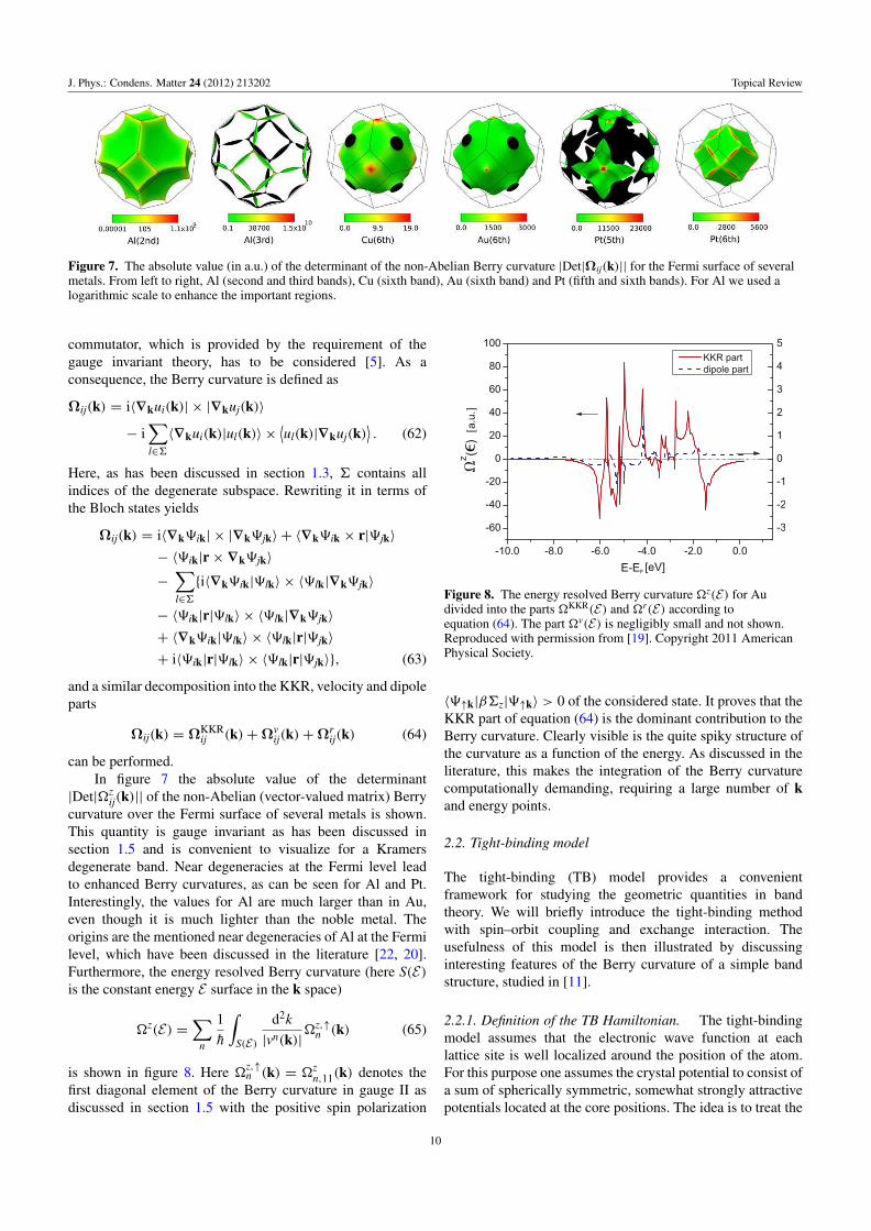
Figure 7. The absolute value (in a.u.) of the determinant of the non-Abelian Berry curvature |Det|Ωij(k)|| for the Fermi surface of severalmetals. From left to right, Al (second and third bands), Cu (sixth band), Au (sixth band) and Pt (fifth and sixth bands). For Al we used alogarithmic scale to enhance the important regions.
commutator, which is provided by the requirement of the
gauge invariant theory, has to be considered [5]. As a
consequence, the Berry curvature is defined as
Ωij(k) = i〈∇kui(k)| × |∇kuj(k)〉
− i∑
l∈6
〈∇kui(k)|ul(k)〉 ×⟨ul(k)|∇kuj(k)
⟩. (62)
Here, as has been discussed in section 1.3, 6 contains all
indices of the degenerate subspace. Rewriting it in terms of
the Bloch states yields
Ωij(k) = i〈∇k9ik| × |∇k9jk〉 + 〈∇k9ik × r|9jk〉− 〈9ik|r × ∇k9jk〉−∑
l∈6
i〈∇k9ik|9lk〉 × 〈9lk|∇k9jk〉
− 〈9ik|r|9lk〉 × 〈9lk|∇k9jk〉+ 〈∇k9ik|9lk〉 × 〈9lk|r|9jk〉+ i〈9ik|r|9lk〉 × 〈9lk|r|9jk〉, (63)
and a similar decomposition into the KKR, velocity and dipole
parts
Ωij(k) = ΩKKRij (k) + Ω
vij(k) + Ω
rij(k) (64)
can be performed.
In figure 7 the absolute value of the determinant
|Det|zij(k)|| of the non-Abelian (vector-valued matrix) Berry
curvature over the Fermi surface of several metals is shown.
This quantity is gauge invariant as has been discussed in
section 1.5 and is convenient to visualize for a Kramers
degenerate band. Near degeneracies at the Fermi level lead
to enhanced Berry curvatures, as can be seen for Al and Pt.
Interestingly, the values for Al are much larger than in Au,
even though it is much lighter than the noble metal. The
origins are the mentioned near degeneracies of Al at the Fermi
level, which have been discussed in the literature [22, 20].
Furthermore, the energy resolved Berry curvature (here S(E )
is the constant energy E surface in the k space)
z(E ) =∑
n
1
h
∫
S(E )
d2k
|vn(k)|z,↑n (k) (65)
is shown in figure 8. Here z,↑n (k) = z
n,11(k) denotes the
first diagonal element of the Berry curvature in gauge II as
discussed in section 1.5 with the positive spin polarization
Figure 8. The energy resolved Berry curvature z(E ) for Audivided into the parts KKR(E ) and r(E ) according toequation (64). The part v(E ) is negligibly small and not shown.Reproduced with permission from [19]. Copyright 2011 AmericanPhysical Society.
〈9↑k|β6z|9↑k〉 > 0 of the considered state. It proves that the
KKR part of equation (64) is the dominant contribution to the
Berry curvature. Clearly visible is the quite spiky structure of
the curvature as a function of the energy. As discussed in the
literature, this makes the integration of the Berry curvature
computationally demanding, requiring a large number of k
and energy points.
2.2. Tight-binding model
The tight-binding (TB) model provides a convenient
framework for studying the geometric quantities in band
theory. We will briefly introduce the tight-binding method
with spin–orbit coupling and exchange interaction. The
usefulness of this model is then illustrated by discussing
interesting features of the Berry curvature of a simple band
structure, studied in [11].
2.2.1. Definition of the TB Hamiltonian. The tight-binding
model assumes that the electronic wave function at each
lattice site is well localized around the position of the atom.
For this purpose one assumes the crystal potential to consist of
a sum of spherically symmetric, somewhat strongly attractive
potentials located at the core positions. The idea is to treat the
10

J. Phys.: Condens. Matter 24 (2012) 213202 Topical Review
overlap matrix elements as a perturbation and consequently
expand the wave function in a basis of atomic orbitals φα(r−R). The ansatz
9nk(r) = 1√NR
∑
R
eikR∑
α
Cnα(k)φα(r − R) (66)
ensures that 9nk fulfils the Bloch theorem with the lattice
vectors R. The simplest case involves neglecting the overlap
matrix elements of the wave function
〈φβ(r − R)|φα(r − R′)〉 ∼ δα,βδR,R′ . (67)
The normalized eigenfunctions in this on-site approximation
are subject to the eigenvalue problem 〈9nk|H|9nk〉 =Enk. The solution to this problem in the tight-binding
formulation of equation (66) requires the diagonalization of
the tight-binding matrix
Hαβ(k) =∑
R,R′eik(R−R′)〈φα(r − R′)|H|φβ(r − R)〉. (68)
Then the coefficients Cnα(k) are obtained as the components
of the eigenvector of this matrix and thus the eigenstates
necessary for the evaluation of the Berry curvature are easily
accessible.
The matrix elements in equation (68) can be parametrized
by the method of Slater and Koster [27]. In order to observe
a nontrivial Berry curvature we need to take into account
spin degrees of freedom. This doubles the number of bands
compared to the spinless case. Within the scope of the
tight-binding model the spin–orbit interaction is treated as a
perturbation
VSOC = h
4m2c2(∇rV(r) × p) S = 2λ
h2LS (69)
to the Hamiltonian. Here a spherically symmetric potential is
assumed and the parameter λ is considered to be small with
respect to the on-site and hopping energies in equation (68).
The matrix elements of this operator have been listed
elsewhere for basis states of p, d and f symmetry [28] in an
on-site approximation, although the formalism presented here
does not require this approximation.
Furthermore, one can use this model to describe
a ferromagnetic material by incorporating an exchange
interaction term. The simplest formulation originates from
the mean-field theory. Without taking into account any
temperature dependence, a constant exchange field is assumed
and the z axis is chosen as the quantization direction
Hxc = −Vxc σ = −Vxcσz, (70)
where Vxc is a positive real number.
2.2.2. Berry curvature. As in the case of the KKR
method discussed in section 2, solving the eigenproblem
of the tight-binding matrix gives the Bloch wave |9nk〉instead of the periodic function |un(k)〉. Hence, one also
needs to consider the two parts, Ωk(k) and Ω
r(k), of the
Berry curvature introduced by equation (60). Exploiting the
on-site approximation of equation (67) and the normalization
condition for the coefficients, one gets the first term for the
Abelian case in a well known form
Ωkn(k) = i 〈∇k9nk| × |∇k9nk〉uc = i∇kC
†n(k) × ∇kCn(k)
= − Im∑
m6=n
C†n(k)∇k
¯H(k)Cm(k)×C†m(k)∇k
¯H(k)Cn(k)
(Enk−Emk)2.
(71)
The second, the dipole term, is given by
Ωrn(k) = ∇k × 〈9nk|r|9nk〉cell = ∇k × (C
†n(k) ¯r Cn(k))
=∑
m6=n
2 Re
[C
†n(k)∇k
¯H(k)Cm(k)
Enk − Emk
× (C†m(k) ¯r Cn(k))
], (72)
where we have introduced the vector-valued matrix ¯r with the
components rαβ = 〈φβ(r)|r|φα(r)〉. Similar to the screened
KKR method, the k derivative of ¯H(k) in the equations above
may be performed analytically and no numerical derivative is
needed.
In the case of degenerate bands, the non-Abelian Berry
curvature Ωij(k) = Ωkij(k) + Ω
rij(k) is expressed in the
following terms (according to section 1.3, 6 contains all
indices of the degenerate subspace):
Ωkij(k) = i
∑
m6∈6
C†i (k)∇k
¯H(k)Cm(k)×C†m(k)∇k
¯H(k)Cj(k)
(Eik−Emk)(Ejk−Emk),
(73)
Ωrij(k) =
∑
m6∈6
[−(C
†i (k) ¯r Cm(k)) × C
†m(k)∇k
¯H(k)Cj(k)
Ejk − Emk
+ C†i (k)∇k
¯H(k)Cm(k)
Eik − Emk
× (C†m(k) ¯r Cj(k))
]
− i∑
l∈6
(C†i (k) ¯r Cl(k)) × (C
†l (k) ¯r Cj(k)). (74)
Here only the last term is not a direct generalization of the
Abelian Berry curvature. Again it is possible to circumvent
the numerical derivative by a summation over all states that
do not belong to the degenerate subspace. The last term does
not involve any derivative, therefore the sum runs only over
the degenerate bands.
2.2.3. Diabolical points. To illustrate the behavior of the
Berry curvature near degeneracies, we present calculations
of a simple band structure using the tight-binding method.
We consider a ferromagnetic simple cubic crystal with
eight bands including one band with s symmetry and three
bands with p symmetry for each spin direction. Due to the
exchange interaction there is no time-reversal symmetry and
the codimension of degeneracies is three.
Regions of the parameter space with a higher symmetry
(e.g. high-symmetry lines in the Brillouin zone) are
more likely to support accidental degeneracies because the
11

J. Phys.: Condens. Matter 24 (2012) 213202 Topical Review
Figure 9. Left: the crossing of some p bands of a ferromagnetic simple cubic band structure near the center of the Brillouin zone. Right:conical intersection of energy surfaces near point P. The z axis represents the energy dispersion of two intersecting bands over an arbitraryplane in k space through the diabolical point. The color scale denotes the spin polarization corresponding to each band.
Figure 10. Left: absolute value of the Berry curvature |Ω| plotted over a plane in k space through the degeneracy point P. Right: inversesquare root of the absolute value, i.e. 1/
√|Ω|.
symmetry possibly reduces the codimension only in this
region. Level crossings on a high-symmetry line in the
Brillouin zone do not necessarily occur on account of
symmetry as long as the bands are not degenerate at points
nearby which have the same symmetry.
As an example, in figure 9 a few bands of the band
structure near the Ŵ point along a high-symmetry line
are plotted. There occur three crossings between different
bands. On the right-hand side, the energy dispersion in a
plane through the degeneracy marked by P is displayed
in order to show the cone shape of the intersection. The
color scale represents the spin polarization 〈9|σz|9〉 of the
corresponding band. Within one band the spin polarization
rapidly changes in the vicinity of the degeneracy. At the
degeneracy itself it jumps due to the cusp of the corresponding
band. However, when passing the intersection along a straight
line in k space and jumping from the lower to the upper band
apparently the spin polarization does not change at all. This
is a clear indication that the character of the two bands is
exchanged at the intersection.
The behavior of the spin polarization near the diabolical
point illustrates how observables are influenced by other
bands nearby. The Berry curvature can be viewed as a measure
of this coupling, which becomes evident from equations (71)
and (72), where a sum over all other bands is performed
weighted by the inverse energy difference. Hence, the Berry
curvature of a single Bloch band generally arises due to
the restriction to this band and it becomes large when other
bands are close. As we have seen before, a degeneracy
produces a singularity of the Berry curvature and the adiabatic
single-band approximation fails.
In our case, the origin of the Berry curvature is the
spin–orbit coupling. Since degenerate or almost degenerate
points in the band structure produce large spin mixing of the
involved bands, a peak in the Berry curvature can also be
understood from this point of view.
As discussed in section 1.4, we would expect the
curvature around the degeneracy to obey the 1/|k − k∗|2 law
of a Coulomb field. The asymptotic behavior becomes evident
when plotting 1/√
|Ω| in a plane in which the degeneracy is
located (see figure 10 with k∗ = (0, 0, kP)). We observe an
absolute value function |k − k∗|, which proves that the Berry
curvature really has the form of the monopole field strength
given by equation (40).
Besides the absolute value we can also examine the
direction of the Berry curvature vector. In figure 11, we
recognize the characteristic monopole field. In the lower band
the monopole is a source, in the upper band a drain, of the
Berry curvature. This has been expected because a monopole
in one band has to be matched by a monopole of opposite
charge in the other band involved in the degeneracy.
In general, we may assign a ‘charge’ g to the monopole
as in equation (42). This charge is quantized to be either
integer or half integer. In order to determine the charge
numerically one could perform a fit of the numerical data with
the monopole field strength. However, there is no reason to
12

J. Phys.: Condens. Matter 24 (2012) 213202 Topical Review
Figure 11. Normalized Berry curvature vector around P (compare figure 9, right panel).
Figure 12. The value of the integral equation (75) over a sphericalsurface for the upper band is plotted against the radius of the sphere.
believe that all directions in k space must be equivalent. Some
distortion in a certain direction might result in ellipsoidal
isosurfaces of |Ω| instead of spherical ones. A different
approach, independent from the coordinate system, exploits
equation (41)∫
V
d3k ∇k ·Ωn(k) =∫
∂V
ds n ·Ωn(k) = 2πm m ∈ Z,
(75)
where the vector n is normal on the bounding surface ∂V of
some arbitrary volume V . Performing the numerical surface
integration causes no problem since the Berry curvature is
analytical on the surface, unlike the case at the degeneracy. So
as to validate this formula, the Berry curvature flux through
a sphere of radius |k − k0| centered at a generic point k0 in
the Brillouin zone near P (see figure 9) is evaluated. This flux
divided by 2π as a function of the sphere’s radius is plotted in
figure 12.
The integral is observed to be quantized to integer
multiples of 2π . When increasing the radius of the sphere
the surface crosses various diabolical points. Each time this
happens the flux jumps by ±2π depending on whether
the charge of the Berry curvature monopole is positive or
negative. According to equation (75), this confirms that
the charges of the monopoles created by the point-like
degeneracies are g = ±1/2. Altogether there are six jumps,
which means there are six diabolical points in the vicinity of
the point P (see figure 9). Two of the monopoles in the upper
band have a negative, the other four a positive, charge of 1/2.
A generic point such as the center of the integration sphere is
chosen to avoid crossing more than one diabolical point at a
time. The deviations from a perfect step function are due to the
discretization of the integral, which increases the error when
the surface crosses a monopole. The step functions also verify
the statement that monopoles are the only possible sources of
the Berry curvature.
Haldane [16] describes the dynamics of these degenera-
cies with respect to the variation of some control parameter,
including the creation of a pair of diabolical points and
their recombination after relative displacement of a reciprocal
lattice vector. In the considered case an obvious choice for the
control parameters would be λ or Vxc, regulating the strength
of spin–orbit coupling or exchange splitting, respectively.
Thus, the tight-binding code provides an excellent tool for
an investigation of the effects connected with the accidental
degeneracy of bands (see for instance, [16]) since one may
scan through a whole range of parameters without consuming
many computational resources and still obtain qualitatively
reliable results.
2.3. Wannier interpolation scheme
The first method developed specifically for calculating the
Berry curvature of Bloch electrons using the full machinery
of the density functional theory (DFT) was based on the
Wannier interpolation code of Marzari et al [29]. As in the
case of the KKR method presented in section 2.1, the essence
of this approach by Wang et al [21] is that it avoids taking
the derivative of the periodic part of the Bloch function
un(r, k) with respect to k numerically by finite differences.
A second almost equally important feature is that it offers
various opportunities to interpolate between different k points
in the Brillouin zone and hence reduces the number of points
at which full ab initio calculations need to be performed.
Note that the formulas, naturally arising in wave packet
dynamics, for the Berry connection and curvature, given by
equations (20) and (21), involve the real space integrals over a
unit cell only. Extending them to cover all space by using the
13

J. Phys.: Condens. Matter 24 (2012) 213202 Topical Review
Wannier functions defined as
|Rn〉 = Vuc
(2π)3
∫
BZ
d3k e−ik·R |9nk〉 , (76)
the Bloch theorem and some care with the algebra, one finds
the following remarkably simple results [21, 30]:
An(k) =∑
R
〈0n| r |Rn〉 eik·R and
Ωn(k) = i∑
R
〈0n| R × r |Rn〉 eik·R.(77)
The matrix elements with respect to the Wannier states,
as usual, involve integrals over all space. These formulas
turn up and play a central role in the method of Wang
et al [21] and make the Wannier interpolation approach
look different from that based on the KKR method, which
makes use of expansions and integration within a single
unit cell only. The lattice sums in equations (77) do not
have convenient convergence properties, as they depend on
the tails of the Wannier functions in real space. Important
to note is the fact that the phase freedom of the Bloch
states allows for an optimization of these tails to reduce
the numerical effort. By now an efficient procedure giving
‘maximally localized’ Wannier functions [29, 30] has been
developed to deal with this issue. Interestingly, in this
procedure matrix elements of both ∇k and r, as in the KKR
method discussed in section 2.1, occur. Reassuringly, it is
found that in both approaches an easy to evaluate matrix
element of ∇k dominates over what is frequently called
the dipole contribution involving matrix elements of r. The
Wannier orbitals are localized but, unlike the orbitals in
the tight-binding method, exact representations of the band
structure of a periodic solid within this method are possible
only for a limited energy range. For metals, its use in modern
first-principle calculations is based on the unique ‘maximally
localized orbitals’ and its power and achievements are well
summarized in [29]. Here we wish to recall only the bare
outline of the new development occasioned by the current
interest in the geometrical and topological features of the
electronic structure of crystals.
The method based on the Wannier interpolation scheme,
fully described in [21], starts with a conventional DFT
calculation of Bloch states |9nq〉 in a certain energy range
and on a selected mesh of q points based on a plane-wave
expansion. Then the matrix elements of various operators may
be constructed with respect to a set of maximally localized
Wannier states |Rn〉. It should be mentioned that generally
these states are distinct from the Wannier states defined in
equation (76) since they are solutions of a procedure to
minimize the real space spread of the Wannier functions [30].
The minimization is always possible due to the freedom
choosing an arbitrary phase in the definition of Bloch states
as mentioned above. In general, this freedom in defining the
Bloch states can be written in terms of a unitary operator. If
we assume a set of Wannier states chosen according to this
procedure, the phase sum of these states
〈r|uWn (k)〉 =
∑
R
e−ik·(r−R) 〈r|Rn〉 (78)
can be defined for an arbitrary k point, which may be at or
in between the first-principle q-point mesh. It can be regarded
as a ‘Wannier gauge’ representation of the periodic part of
a Bloch state but they are generally no eigenstates of the
k-dependent Hamiltonian. In the following one has to evaluate
the matrix elements with respect to the constructed states
HWnm(k) =
∑
R
e+ik·R 〈0n| H |Rm〉 ,
∇HWnm(k) =
∑
R
e+ik·RiR 〈0n| H |Rm〉 ,
AWnm(k) =
∑
R
e+ik·R 〈0n| r |Rm〉 ,
ΩWnm(k) = i
∑
R
e+ik·R 〈0n| R × r |Rm〉 .
(79)
Actually, all of them are given in the same ‘Wannier gauge’.
The indices n and m refer to the full bundle of Wannier states
selected to represent the real bands up to a certain energy
above the Fermi level.
The next step is to find unitary matrices ¯U(k) such that
¯U†(k) ¯H
W(k) ¯U(k) = ¯H
H(k) with
HHnm(k) = Enkδnm, (80)
where the eigenvalues Enk should agree with the first-principle
dispersion relation of the bands chosen to be represented. The
corresponding eigenfunctions
|uHn (k)〉 =
∑
m
Unm(k)|uWm (k)〉 (81)
should reproduce the periodic part of these states.
Thus, |uHn (k)〉 can be used to evaluate equations (20)
and (21) for the Berry connection and the curvature in the
standard way. However, such direct calculations are precisely
not what one would like to do. The point of Wang et al is that
the above preamble offers an alternative. Namely, the unitary
transformation ¯U(k) transforms all states and operators from
the ‘Wannier gauge’ to another gauge which is called the
‘Hamiltonian (H) gauge’ and one can transform all the easy to
evaluate ‘Wannier gauge’ operators in equation (79) into their
‘Hamiltonian gauge’ form. Of course, ΩHnm(k) is of particular
interest. Unfortunately, due to the k dependence of Unm(k) the
form of equations (20) and (21) is not covariant under such a
transformation. For instance, the connection is given by
AH = U†AWU + iU†∇U = A
H + iU†∇U, (82)
where for clarity the momentum dependency has been
dropped as we will mainly do within this section. All products
are matrix multiplications and the gradient is taken with
respect to k. A similar, but more complicated formula can
be derived for ΩH. The matrices A
H,Ω
H, and H
Hdenote
the covariant components, that is to say the part of the
transformed operator which does not contain U†∇U, of AH
and HH, respectively. If we write ΩH = U†
ΩWU and
DHnm = (U†
∇U)nm = (U†∇HWU)nm
Em − En
(1 − δnm), (83)
14

J. Phys.: Condens. Matter 24 (2012) 213202 Topical Review
Figure 13. Left: Berry curvature z(k) of Fe along symmetry lines with a decomposition into three different contributions of equation (84)(note the logarithmic scale). Right: Fermi surface in the (010) plane (solid lines) and the total Berry curvature −z(k) in atomic units (colormap). Reproduced with permission from [21]. Copyright 2006 American Physical Society.
the final formula for the total Berry curvature Ω(k) =∑nfnΩn(k), including the sum over all occupied states, reads
as follows:
Ω(k) =∑
n
fnΩHnn +
∑
n,m
(fm − fn) DHnm × A
Hmn + Ω
DD, (84)
where the last term takes the form
ΩDD = i/2
∑
n,m
(fn − fm)(U†
∇HWU)nm × (U†∇HWU)mn
(Em − En)2.
(85)
Here fn ≡ fn(k) and fm ≡ fm(k) are the equilibrium
distribution functions for bands n and m, respectively. The
sums in equation (84) run over all Wannier states used for an
accurate description of the occupied states. Interestingly, this
is the standard form of the Berry curvature for a Hamiltonian
which depends parametrically on k and it also shows up as
one of the contributions in the KKR and the tight-binding
approaches discussed in sections 2.1 and 2.2. Reassuringly,
computations by all three methods find the contribution
from such terms as equation (85) dominant and almost
exclusively responsible for the spiky features as functions of
k. As noted in the introduction, these features originate from
band crossings or avoided crossings and have a variety of
interesting physical consequences.
For instance, the Berry curvature calculated by Wang
et al [21, 31], shown in figure 13, leads directly to a
good quantitative account of the intrinsic contribution to the
anomalous Hall effect in Fe. The left panel of figure 13
shows the decomposition of the Berry curvature in different
contributions arising from the expansion of the states into
a Wannier basis (see equation (84)). Noting the logarithmic
scale, it is evident that the dominant contribution stems from
the Berry curvature ΩDD(k) of the k-dependent Hamiltonian
HH(k) according to equation (85). The other terms including
matrix elements of the position operator r are negligible,
which is similar to what turned out to be the case within the
KKR method. Further applications of the considered method
to the cases of fcc Ni and hcp Co [31, 32] are equally
impressive.
2.4. Kubo formula
2.4.1. Anomalous Hall conductivity and the Berry curvature.
Most conventional approaches to the electronic transport insolids are based on the very general linear response theoryof Kubo [33]. Indeed, the first insight into the cause ofthe anomalous Hall effect by Karplus and Luttinger [34]was gained by deploying the Kubo formula for a simplemodel Hamiltonian of electrons with spin. In this sectionwe review briefly the first-principle implementation of theKubo formula in aid of calculating the Berry curvature. Thesimple observation which makes this possible is that boththe semiclassical description and the Kubo formula approachyield the same expression for the intrinsic contribution to theanomalous Hall conductivity (AHC). Hence, by comparingthe two, a Kubo-like expression for the Berry curvature canbe extracted. Here we examine the formal connection betweenthe two formulas for the Berry curvature and demonstratethat they are equivalent, as was mentioned already by Wanget al [21].
The Kubo formula for the AHC in the static limit fordisorder-free noninteracting electrons is given by [35]
σxy = e2h
∫
BZ
d3k
(2π)3
∑
n
∑
m6=n
fn(k)
× Im[〈9nk|v|9mk〉 × 〈9mk|v|9nk〉]z
(Enk − Emk)2, (86)
whereas in the semiclassical approach it is expressed in termsof the Berry curvature [7, 14, 34, 41]
σxy = −e2
h
∑
n
∫
BZ
d3k
(2π)3fn(k)z
n(k). (87)
Assuming the equivalence of the two approaches, acomparison of equations (86) and (87) yields a Kubo-likeformula for the Berry curvature. However, the equivalence isnot a priori evident and has to be proven, which will be donein the following.
The starting point is the Berry curvature written in termsof the periodic part of the Bloch function
Ωn(k) = i 〈∇kun(k)| × |∇kun(k)〉 . (88)
15

J. Phys.: Condens. Matter 24 (2012) 213202 Topical Review
Let us follow the route given by Berry [3] to rewrite this
expression. Introducing the completeness relation with respect
to the N present bands, 1 =∑N
m=1|um〉〈um|, excluding the
vanishing term with m = n and using the relation
〈∇un(k)|um(k)〉 = 〈un(k)| ∇kH(k) |um(k)〉Enk − Emk
, (89)
which follows from 〈un(k)|H(k)|um(k)〉 = Emk〈un(k)|um(k)〉= 0, yields
Ωn(k) =
i∑
m6=n
〈un(k)| ∇kH(k) |um(k)〉 × 〈um(k)|∇kH(k)|un(k)〉(Enk − Emk)2
.
(90)
If we reformulate it with respect to the Bloch functions
Ωn(k) = i∑
m6=n
〈9nk|eikr∇kH(k)e−ikr|9mk〉
× 〈9mk|eikr∇kH(k)e−ikr|9nk〉
× (Enk − Emk)2−1
(91)
and use the relations
H(k) = e−ikrHeikr, (92)
∇kH(k) = ie−ikr[Hr − rH
]eikr = h e−ikrveikr, (93)
we end up with a Kubo-like formula widely used in the
literature [37, 38]
Ωn(k) = ih2∑
m6=n
〈9nk|v|9mk〉 × 〈9mk|v|9nk〉(Enk − Emk)2
. (94)
This formula proves the equivalence of the two approaches
for calculating the AHC as given by equations (86) and
(87). In principle, all occupied and unoccupied states have to
be accounted for in the sum of equation (94). However, in
practice only states with energies close to Enk play a role. An
important feature of this form is that it is expressed in terms
of the off-diagonal matrix elements of the velocity operator
with respect to the Bloch states. To deal with them a technique
was adopted, which served well for computing the optical
conductivities [39, 40], where the same matrix elements have
been required.
The first ab initio calculation of the Berry curvature was
actually performed for SrRuO3 by Fang et al [36] using
equation (94). The authors nicely illustrate the existence of
a magnetic monopole in the crystal momentum space, which
is shown in figure 14. The origin of this sharp structure
is the near degeneracy of bands. It acts as a magnetic
monopole. A similar effect was found for Fe by Yao et al [41].
They demonstrate that for k points near the spin–orbit
driven avoided crossings of the bands the Berry curvature
is extremely enhanced as shown in figure 15. In addition,
the agreement between the right panels of figures 13 and 15
shows impressively the equivalence between the two different
methods.
Figure 14. Calculated Berry curvature (in [36] called flux bz)z(k) =
∑n∈t2g
zn(k) distribution in k space for t2g bands as a
function of (kx, ky) with kz = 0 for SrRuO3 with cubic structure.Reproduced with permission from [36]. Copyright 2003 AAAS.
2.4.2. Spin Hall conductivity and the Berry curvature. Of
course, the fact that the results of the semiclassical transport
theory and the quantum mechanical Kubo formula agree
exactly, as was shown above, is surprising. In general, it
cannot be expected for all transport coefficients. Indeed, as
we shall now demonstrate, the situation is quite different for
the spin Hall conductivity.
Evidently, the Kubo approach is readily adopted to
calculate the spin-current response to an external electric field
E. Although there is still a controversy about an expression
for the spin-current operator to be taken [42–45], frequently
the following tensor product of the relativistic spin operator
βΣ and the velocity operator v is used:
JSpin = βΣ ⊗ v, βΣ =(σ 0
0 −σ
). (95)
Furthermore, the symmetrized version of the tensor product
is often used in literature and the spin-current response is
calculated as the expectation value of the operator JSpin.
However, within the Dirac approach we have
v = cα = c
(0 σ
σ 0
)and
β6ivj − vjβ6i = 0, if i 6= j.
(96)
Similar to the formula for the charge Hall conductivity, one
finds for the spin Hall conductivity with spin polarization in
the z direction [43, 37, 38]
σ zxy = e2
h
∑
k,n
σ zxy;n(k)fn(k), (97)
where the k and band resolved conductivity σ zxy;n(k) in the
framework of the Kubo formula (Kubo) is given by
σ zxy;n(k)Kubo =
− h2∑
m6=n
Im[〈9nk|β6zvx|9mk〉〈9mk|vy|9nk〉](Enk − Emk)2
. (98)
16

J. Phys.: Condens. Matter 24 (2012) 213202 Topical Review
Figure 15. Left: band structure of bulk Fe near Fermi energy (upper panel) and Berry curvature z(k) (lower panel) along symmetry lines.Right: Fermi surface in (010) plane (solid lines) and Berry curvature −z(k) in atomic units (color map). Reproduced with permissionfrom [41]. Copyright 2004 American Physical Society.
In the literature, this quantity is sometimes even called spin
Berry curvature [38], analogously to the AHE. This notation
is misleading and should not be used.
Let us tackle the same problem from the point of view of
the semiclassical theory (sc). This suggests that one should
take the velocity in equations (95) to be the anomalous
velocity given by equation (11). This argument leads to [5,
42]
σ zxy;n(k)sc = Tr[ ¯S
z
n(k) ¯z
n(k)]. (99)
Here ( ¯Sz
n(k))ij = 〈9nik|β6z|9njk〉 is the spin matrix for a
Kramers pair labeled by i, j and ¯z
n(k) is the non-Abelian
Berry curvature [19] introduced in section 1.3. The point
we wish to make here is that this formula is not equivalent
to the Kubo form in equation (98). The reason is that
the band off-diagonal terms of the spin matrix were
neglected in the derivation from the wave packet dynamics
of equation (99) [5].
Evidently, σ zxy;n(k)Kubo cannot be written as a single-band
expression, in contrast to the case of the AHC, which turned
out to be exactly the conventional Berry curvature (see
section 2.4.1). The contributions of equation (98) which were
neglected in equation (99) are of quantum mechanical origin
and are not accounted for in the semiclassical derivation.
Culcer et al [42] tackled the problem and identified the
neglected contributions, without giving up the wave packet
idea, as spin and torque dipole terms. Nevertheless, it was
shown that under certain approximations a semiclassical
description may result in quantitatively comparable results to
the Kubo approach [19]. This will be discussed in section 3.
3. Intrinsic contribution to the charge and spinconductivity in metals
Here we discuss applications of the computational methods
for the Berry curvature discussed in section 2. We will focus
on first-principle calculations of the anomalous and spin Hall
conductivities. The anomalous Nernst conductivity, closely
related to it, will be also discussed briefly.
The first ab initio studies of the AHE, based on
equation (87) with Ωn(k) defined by equation (94), were
reported in [36, 46]. As is well known, the conventional
expression for the Hall resistivity
ρxy = R0Bz + 4πRsMz (100)
(where Bz is the magnetic field in the z direction and R0
and Rs are the normal and the anomalous Hall coefficient,
respectively) assumes a monotonic behavior of ρxy as well
as σxy as a function of the magnetization M. By means
of first-principle calculations based on the pseudopotential
method (STATE code), Fang et al [36] have shown that the
unconventional nonmonotonic behavior of the AHC measured
in SrRuO3 (figure 16, left) is induced by the presence of a
magnetic monopole (MM) in momentum space (see figure 14
and the corresponding discussion in section 2.4.1). The
existence of MMs causes the sharp and spiky structure of the
AHC as a function of the Fermi-level position, shown in the
right panel of figure 16. At the self-consistently determined
Fermi level, the calculated value σxy = −60 ( cm)−1 is
comparable with the experimentally observed conductivity
of about −100 ( cm)−1. Obviously, a small change in the
Fermi level would cause dramatic changes in the resulting
AHC. Indeed, as was shown in [46], the calculated AHC
of ferromagnetic Gd2Mo2O7 and Nd2Mo2O7 is strongly
changed by the choice of the Coulomb repulsion U varied in
the used mean-field Hartree–Fock approach.
A year later, results for the intrinsic AHC in ferromag-
netic bcc Fe, based on the full-potential linearized augmented
plane-wave method (WIEN2K code), were published [41].
The authors used the same Kubo formula approach to describe
the transversal transport. In particular, a close agreement
between theory, σxy = 751 ( cm)−1, and experiment, σxy =1032 ( cm)−1, was found, that points to the dominance of
the intrinsic contribution in Fe. A slow convergence of the
calculated value for the AHC with respect to the number
of k points was reported. The reason for the convergence
17
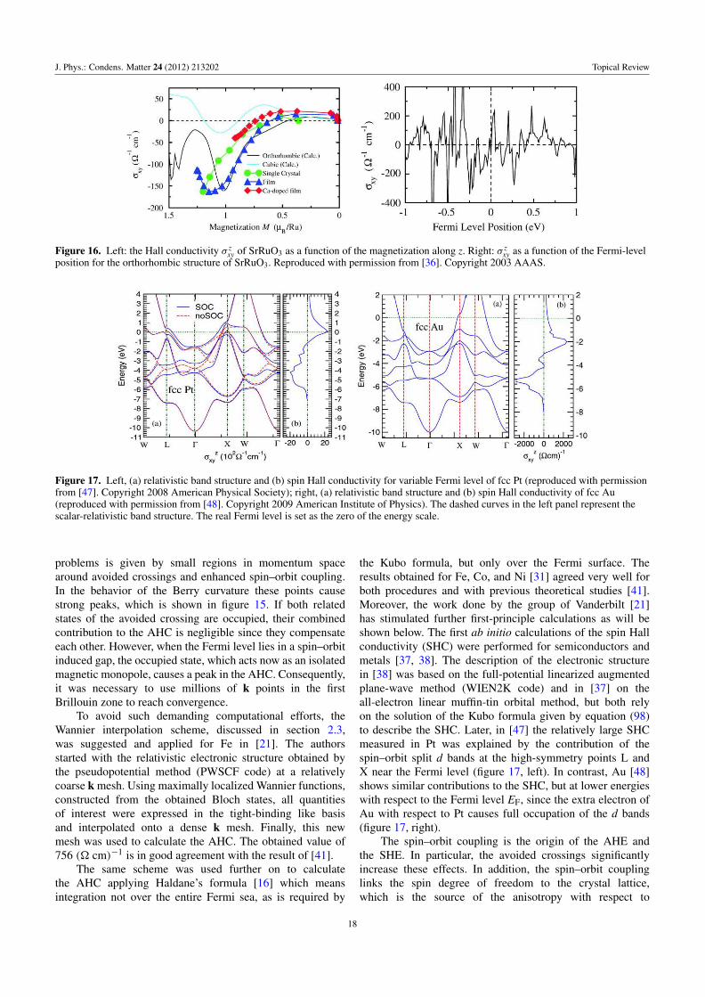
J. Phys.: Condens. Matter 24 (2012) 213202 Topical Review
Figure 16. Left: the Hall conductivity σ zxy of SrRuO3 as a function of the magnetization along z. Right: σ z
xy as a function of the Fermi-levelposition for the orthorhombic structure of SrRuO3. Reproduced with permission from [36]. Copyright 2003 AAAS.
Figure 17. Left, (a) relativistic band structure and (b) spin Hall conductivity for variable Fermi level of fcc Pt (reproduced with permissionfrom [47]. Copyright 2008 American Physical Society); right, (a) relativistic band structure and (b) spin Hall conductivity of fcc Au(reproduced with permission from [48]. Copyright 2009 American Institute of Physics). The dashed curves in the left panel represent thescalar-relativistic band structure. The real Fermi level is set as the zero of the energy scale.
problems is given by small regions in momentum spacearound avoided crossings and enhanced spin–orbit coupling.In the behavior of the Berry curvature these points causestrong peaks, which is shown in figure 15. If both relatedstates of the avoided crossing are occupied, their combinedcontribution to the AHC is negligible since they compensateeach other. However, when the Fermi level lies in a spin–orbitinduced gap, the occupied state, which acts now as an isolatedmagnetic monopole, causes a peak in the AHC. Consequently,it was necessary to use millions of k points in the firstBrillouin zone to reach convergence.
To avoid such demanding computational efforts, theWannier interpolation scheme, discussed in section 2.3,was suggested and applied for Fe in [21]. The authorsstarted with the relativistic electronic structure obtained bythe pseudopotential method (PWSCF code) at a relativelycoarse k mesh. Using maximally localized Wannier functions,constructed from the obtained Bloch states, all quantitiesof interest were expressed in the tight-binding like basisand interpolated onto a dense k mesh. Finally, this newmesh was used to calculate the AHC. The obtained value of756 ( cm)−1 is in good agreement with the result of [41].
The same scheme was used further on to calculatethe AHC applying Haldane’s formula [16] which meansintegration not over the entire Fermi sea, as is required by
the Kubo formula, but only over the Fermi surface. Theresults obtained for Fe, Co, and Ni [31] agreed very well forboth procedures and with previous theoretical studies [41].Moreover, the work done by the group of Vanderbilt [21]has stimulated further first-principle calculations as will beshown below. The first ab initio calculations of the spin Hallconductivity (SHC) were performed for semiconductors andmetals [37, 38]. The description of the electronic structurein [38] was based on the full-potential linearized augmentedplane-wave method (WIEN2K code) and in [37] on theall-electron linear muffin-tin orbital method, but both relyon the solution of the Kubo formula given by equation (98)to describe the SHC. Later, in [47] the relatively large SHCmeasured in Pt was explained by the contribution of thespin–orbit split d bands at the high-symmetry points L andX near the Fermi level (figure 17, left). In contrast, Au [48]shows similar contributions to the SHC, but at lower energieswith respect to the Fermi level EF, since the extra electron ofAu with respect to Pt causes full occupation of the d bands(figure 17, right).
The spin–orbit coupling is the origin of the AHE andthe SHE. In particular, the avoided crossings significantlyincrease these effects. In addition, the spin–orbit couplinglinks the spin degree of freedom to the crystal lattice,which is the source of the anisotropy with respect to
18

J. Phys.: Condens. Matter 24 (2012) 213202 Topical Review
Figure 18. Spin Hall conductivities σ xyz and σ z
xy for several hcp nonmagnetic metals and for antiferromagnetic Cr. Reproduced withpermission from [49]. Copyright 2010 American Physical Society.
Figure 19. The intrinsic spin Hall conductivity for fcc Pt (left) and Au (right) [19]. The Fermi level is set to zero on the energy scale.Reproduced with permission from [19]. Copyright 2011 American Physical Society.
the chosen quantization axis; this means σ xyz and σ z
xy may
differ. This was demonstrated first for the AHE in hcp
Co [32] and later for the SHE in several nonmagnetic hcp
metals [49] (figure 18). Here, the pseudopotential method
(PWSCF code) and the full-potential linearized augmented
plane-wave method (FLEUR code) were used for the AHE
and SHE, respectively. To reduce the computational efforts,
the Berry curvature calculations were based on the Wannier
interpolation scheme according to [21]. These methods were
applied to several situations in ordered alloys [50] where the
anisotropy of the AHC [51] was discussed as well and the
roles of spin-conserving and non-spin-conserving parts of the
SOC were discussed in detail [52]. Very recently the same
group calculated the scattering-independent contribution to
the side jump mechanism for the anomalous Hall effect [53].
The used approach is based on a model assuming short-range
uncorrelated disorder and involves the Berry connection of the
Bloch states as an essential part [54].
Finally, an approach for calculating the SHC based on
the KKR method was proposed ([19], section 2.1). For
the description of the transversal spin transport the authors
applied an approach different from the widely used Kubo
formula. Their calculations are based on the expression for
the SHC in the non-Abelian case suggested in [5]. This
expression was simplified further by the approximation that
the expectation value of the β6z operator is assumed to
be +1 and −1 for the two spin degenerate states, arising
in nonmagnetic crystals with inversion symmetry. Thus, the
semiclassical treatment was reduced to the two current model
with the final expression for the SHC in terms of the usual
formula for the AHC at zero temperature
σ zxy = e2
h(2π)3
∫ EF
dE z(E ), (101)
where z(E ) is defined by equation (65). The spin Hall
conductivities σ zxy(E ) considered for a variable Fermi level,
and calculated for Pt and Au in such an approach (figure 19),
are quantitatively in good agreement with the ones obtained
by the Kubo-like formula (see figure 17).Related to the already discussed calculation of the
intrinsic spin and anomalous Hall conductivities is the
intrinsic mechanism of the anomalous Nernst effect. It is
driven by an applied thermal gradient instead of the applied
electric field. The two driving forces are of physically
different nature. The electric field is a mechanical force in
contrast to the statistical force of a temperature gradient.
Nevertheless, as was shown by Xiao et al [55], the final
expression for the anomalous Nernst conductivity αxy at low
temperatures is simply given by the Mott relation
αxy = π2
3
k2BT
eσ ′
xy(EF). (102)
Here σ ′xy(EF) is the first energy derivative at EF of the
intrinsic anomalous Hall conductivity, defined in terms of
19

J. Phys.: Condens. Matter 24 (2012) 213202 Topical Review
Figure 20. The intrinsic anomalous Nernst conductivity (dividedby the temperature T) of the CuCr2Se4−xBrx alloy as a function ofthe Br content x. Reproduced with permission from [55]. Copyright2006 American Physical Society.
the Berry curvature in equation (87). All the above methods
to calculate the Berry curvature can be applied to compute
the anomalous Nernst conductivity as well. In figure 20 a
comparison between experimental results and first-principle
calculations for the alloy CuCr2Se4−xBrx are shown. The
concentration dependence is described by using a rigid band
model. The agreement is relatively good despite the fact
that the experiment cannot resolve the peak–valley structure
around x = 0.2.
4. De Haas–van Alphen oscillation and the Berryphases
Other phenomena related to the topic of this review are
various quantum oscillations. For their proper description
typically the Berry phase accumulated along a closed orbit in
parameter space is needed, which can be expressed via the
Berry curvature of the system. For instance, in the case of
the de Haas–van Alphen effect, the semiclassical formula for
the quantized energies of the Landau levels includes a term
involving the Berry phase of the corresponding orbits in k
space. This was pointed out by Mikitik and Sharlai [56, 57],
who have discussed a number of interesting experiments in
these terms [58, 59]. They argue that the quasiparticles which
move along closed orbits in response to an external magnetic
field B are wave packets, in the sense of the semiclassical
theory, and therefore their semiclassical equations (8) and
(9) are subject to corrections arising from Berry phases
and curvatures. In short, a closed orbit is defined by the
requirement that the energy of the wave packet Enk − M(k)B
is equal to E = constant for all k along the orbit. Here M(k)
is the spin plus the orbital magnetic moment of the electron
along the path. Then the Bohr–Sommerfeld quantization
condition for E = Eν to be a Landau level is [1, 57, 60]
S(Eν, kz) = 2π heBz
(ν + 1
2− γn
2π
), (103)
where S(Eν, kz) is the area enclosed by the orbit in k space.
The Berry phase accumulated along the orbit labeled by C is
given by
γn =∮
C
dk · An(k) =∫∫
Sc
dS ·Ωn(k), (104)
where Sc is any surface in k space whose boundary is C.
Clearly, the presence of the orbital magnetization in the theory
indicates that the change of the band energy due to spin and
orbital motion is taken into account. This important fact is
more evident if equation (103) is recast as
S0(Enk, kz) = 2π heBz
×(
ν + 1
2− γn
2π− 1
2π
∮
C0
Mz(k) dk
|∂Enk/∂k⊥|
),
(105)
where S0(Enk, kz) is the area enclosed by an orbit C0 on an
iso-energetic surface of the actual band structure. From the
point of view of analyzing the high quality data available
from de Haas–van Alphen measurements, the physical content
of the above formula is of considerable general interest,
and shows the necessary correction of the common theory.
However, to calculate the loop integral in equation (105) for
the general case with spin–orbit coupling is a real challenge,
which has been, so far, only partially implemented6.
The full theory has already been presented by Roth in
1966 [61], although never applied to analyze experimental
data. Only recently the formulas have been revisited in view
of the new light cast on them by advances in describing wave
packets driven by external fields and the associated Berry
phases.
To highlight the significance of the Berry phase and
curvature in the present context, we shall now consider the
simple case where the spin, and therefore the spin–orbit
coupling, is altogether neglected and it is assumed that the
system is time-reversal and inversion symmetric. In this case
one might think that the Berry phase would vanish since the
Berry curvature is zero over the full Brillouin zone. However,
as was shown by Mikitik and Sharlai [56, 57], this is not true
if the semiclassical orbit encloses a line of degeneracy. As was
shown in [58, 59] for several materials, such lines exist in the
absence of spin–orbit coupling and have a significant effect on
the observable de Haas–van Alphen frequencies.
Here we focus on two hexagonal systems, Mg and Tl, and
discuss the results for γn, given by equation (104), obtained
with the KKR method [22, 19]. In figure 21 the band structure
of Mg along the ŴM direction clearly shows an accidental
degeneracy, which is actually part of a full line in the kz = 0
plane as shown in the right panel of figure 21. Furthermore,
this line is enclosed by one sheet of the Fermi surface, which
allows us to study the effect. If the magnetic field is applied in
different directions as shown in figure 22, orbits either enclose
the line of degeneracy, as in the case shown in red, or they do
not, shown in black. We have evaluated the integrals over a
selection of those loops numerically and found γn = π for
all orbits which enclose the line and γn = 0 for all those
which do not. The important fact is that the integral value
6 See for example [63] and citations [9–30] in [62].
20

J. Phys.: Condens. Matter 24 (2012) 213202 Topical Review
Figure 21. Left panel: band structure of hcp Mg along the ŴM direction. The accidental degeneracy of two bands is part of a line ofdegeneracy in the kz = 0 plane. The inset shows the lifting of the degeneracy due to spin–orbit coupling. Right panel: the full line ofdegeneracy which is enclosed by the Fermi surface of the second band.
Figure 22. Fermi surfaces for Cu (a) and Mg (b) with extremal orbits for different directions of the applied magnetic field. For Tl (c) aconstant energy surface slightly above the Fermi energy (EF + 0.02 Ryd) was chosen to create extremal orbits enclosing a line of contactpoints. These orbits on tiny ellipsoids in the ŴM direction are shown in red and black for B fields parallel and perpendicular to the hcp baseplane respectively. The lines of degeneracy are shown as blue dashed lines.
is independent of the actual form of the loop. The effect is
topological since only whether the line penetrates the orbit or
not is relevant. This result dramatically affects the analysis
of de Haas–van Alphen experiments since the quantization
condition of equation (103) will be either
S(Eν, kz) = 2π heBzν (106)
or
S(Eν, kz) = 2π heBz(ν + 12 ) (107)
depending on whether the orbit encloses a line of degeneracies
or not, respectively.
Clearly, what happens to such lines of degeneracies in
the presence of spin and spin–orbit coupling is an interesting
and fundamental question, since in that case the bands
are formed from states that are Kramers doublets and two
such doublets are infinitely unlikely to be degenerate. In
the limit of small spin–orbit coupling this question was
investigated by Mikitik and Sharlai [62]. They found that the
Berry phase contribution becomes zero, but for nonmagnetic
inversion symmetric systems there is a contribution to the area
enclosed by a Landau orbit arising from the magnetization
part of equation (105). However, the case of strong spin–orbit
coupling remains an open problem.
5. Conclusion
In the presence of a periodic crystal potential the free electron
spectrum Ek = h2k2
2mbreaks up into bands with nontrivial
dispersion relations Enk. It turns out that the adiabatic
dynamics of wave packets, constructed by superposition
of all k states but a limited number of bands n, features
a Berry connection An(k) and a corresponding curvature
Ωn(k), which account for the influence of the neglected
bands [6, 7]. Moreover, these geometrical properties of the
band structure play an essential role in describing a number
of important physical phenomena such as spin and charge
transport, electric polarization and orbital magnetization [1].
What makes these remarkable developments particularly
interesting from the point of view of first-principle electronic
structure calculations is the fact that the curvature Ωn(k) is a
very rapidly varying function of k and it depends on intricate
details of the band structure. Consequently, devising methods
for computing Ωn(k) have recently become a very active
21

J. Phys.: Condens. Matter 24 (2012) 213202 Topical Review
field of research. In this paper we sketched three approaches
to the problem: one is based on multiple scattering theory
(KKR, similarly LMTO), another one on the Wannier function
representation of first-principle bands and the third one on
direct evaluation of a Kubo-like formula. We pointed out
the differences and highlighted the similarities in the way
the derivatives with respect to the wave vector k enter the
problem. We stressed the importance of level crossings which
give rise to curvatures Ωn(k) whose k dependence is that of
the Dirac monopole and the more exotic avoided crossings of
Kramers degenerate bands whose curvature is a non-Abelian
gauge field. As illustrations of results by the various methods,
we presented calculations of the intrinsic contribution to the
anomalous and spin Hall conductivity and the Berry curvature
for a variety of systems as well as the manifestation of the
Berry phase in de Haas–van Alphen oscillations.
In that review we concentrated on the Berry curvature
caused by the parameter k in the Hamiltonian for Bloch
electrons. However, from the general point of view any slowly
changing parameter in a Hamiltonian causes curvatures which
might be of interest in future considerations. From that
perspective, curvatures associated with spatial or temporal
parameters will represent new computational challenges.
Very recently, after finalizing this manuscript, another
method calculating the Berry curvature was published [64]. It
is based on a finite-differences approach within the augmented
spherical wave scheme. The method was originally developed
for calculating directly the Z2 invariants of topological
insulators and not for expressing the Berry curvature k-point
by k-point [65, 66]. This is the reason why we missed it. We
would like to thank Professor Jurgen Kubler for discussing
this new method with us.
Acknowledgments
One of us (BLG) would like to thank Professor Michael Berry
for many fruitful conversations on the topic of this article. MG
acknowledges support from the German Research Foundation
(DFG) via a Research Fellowship (GR 3838/1-1). In addition,
this work was supported by the DFG via SFB 762.
References
[1] Xiao D, Chang M-C and Niu Q 2010 Berry phase effects onelectronic properties Rev. Mod. Phys. 82 1959
[2] Marder M P 2000 Condensed Matter Physics (New York:Wiley)
[3] Berry M V 1984 Quantal phase factors accompanyingadiabatic changes Proc. R. Soc. A 392 45
[4] Culcer D, Yao Y and Niu Q 2005 Coherent wave-packetevolution in coupled bands Phys. Rev. B 72 085110
[5] Shindou R and Imura K-I 2005 Noncommutative geometryand non-Abelian Berry phase in the wave-packet dynamicsof Bloch electrons Nucl. Phys. B 720 399–435
[6] Wilczek F and Zee A 1984 Appearance of gauge structure insimple dynamical systems Phys. Rev. Lett. 52 2111
[7] Sundaram G and Niu Q 1999 Wave-packet dynamics in slowlyperturbed crystals: gradient corrections and Berry-phaseeffects Phys. Rev. B 59 14915
[8] Kramers H A 1930 General theory of paramagnetic rotation incrystals Proc. R. Acad. Sci. Amsterdam 33 959
[9] Elliott R J 1954 Theory of the effect of spin–orbit coupling onmagnetic resonance in some semiconductors Phys. Rev.
96 266[10] Berry M V and Wilkinson M 1984 Diabolical points in the
spectra of triangles Proc. R. Soc. A 392 15[11] Pientka F 2010 Geometrical concepts in the band theory of
solids Diploma Thesis University Halle-Wittenberg http://www.physik.uni-halle.de/theorie/ag/qtfk/mitarbeiter/pientka/
[12] Hals K M D, Nguyen A K, Waintal X and Brataas A 2010Effective magnetic monopoles and universal conductancefluctuations Phys. Rev. Lett. 105 207204
[13] Dirac P A M 1948 The theory of magnetic poles Phys. Rev.
74 817[14] Thouless D J, Kohmoto M, Nightingale M P and
den Nijs M 1982 Quantized Hall conductance in atwo-dimensional periodic potential Phys. Rev. Lett. 49 405
[15] Simon B 1983 Holonomy, the quantum adiabatic theorem, andBerry’s phase Phys. Rev. Lett. 51 2167
[16] Haldane F D M 2004 Berry curvature on the Fermi surface:anomalous Hall effect as a topological Fermi-liquidproperty Phys. Rev. Lett. 93 206602
[17] von Neumann J and Wigner E 1929 Uber das verhalten voneigenwerten bei adiabatischen prozessen Phys. Z. 30 467
[18] Bohm A, Mostafazadeh A, Koizumi H, Niu Q andZwanziger J 2003 The Geometric Phase in Quantum
Systems (Berlin: Springer)[19] Gradhand M, Fedorov D V, Pientka F, Zahn P, Mertig I and
Gyorffy B L 2011 On calculating the Berry curvature ofBloch electrons using the KKR method Phys. Rev. B84 075113
[20] Fabian J and Das Sarma S 1998 Spin relaxation of conductionelectrons in polyvalent metals: theory and a realisticcalculation Phys. Rev. Lett. 81 5624
[21] Wang X, Yates J R, Souza I and Vanderbilt D 2006 Ab initio
calculation of the anomalous Hall conductivity by Wannierinterpolation Phys. Rev. B 74 195118
[22] Gradhand M, Czerner M, Fedorov D V, Zahn P,Yavorsky B Yu, Szunyogh L and Mertig I 2009 Spinpolarization on Fermi surfaces of metals by the KKRmethod Phys. Rev. B 80 224413
[23] Pientka F, Gradhand M, Fedorov D V, Mertig I andGyorffy B L 2012 Gauge freedom for degenerate Blochstates Phys. Rev. B submitted
[24] Zeller R, Dederichs P H, Ujfalussy B, Szunyogh L andWeinberger P 1995 Theory and convergence properties ofthe screened Korringa–Kohn–Rostoker method Phys. Rev.
B 52 8807[25] Szunyogh L, Ujfalussy B, Weinberger P and Kollar J 1994
Self-consistent localized KKR scheme for surfaces andinterfaces Phys. Rev. B 49 2721
[26] Strange P 1998 Relativistic Quantum Mechanics with
Applications in Condensed Matter and Atomic Physics
(Cambridge: Cambridge University Press)[27] Slater J C and Koster G F 1954 Simplified LCAO method for
the periodic potential problem Phys. Rev. 94 1498[28] Jones M D and Albers R C 2009 Spin–orbit coupling in an
f-electron tight-binding model: electronic properties of Th,U, and Pu Phys. Rev. B 79 045107
[29] Marzari N, Souza I and Vanderbilt D 2003 An introduction tomaximally-localized wannier functions Psi-k Newsletter
57 129 (Scientific Highlight of the Month) http://www.psi-k.org/newsletters/News 57/Highlight 57.pdf
[30] Marzari N and Vanderbilt D 1997 Maximally localizedgeneralized Wannier functions for composite energy bandsPhys. Rev. B 56 12847
[31] Wang X, Vanderbilt D, Yates J R and Souza I 2007Fermi-surface calculation of the anomalous Hallconductivity Phys. Rev. B 76 195109
22

J. Phys.: Condens. Matter 24 (2012) 213202 Topical Review
[32] Roman E, Mokrousov Y and Souza I 2009 Orientationdependence of the intrinsic anomalous Hall effect in hcpCobalt Phys. Rev. Lett. 103 097203
[33] Kubo R 1957 Statistical–mechanical theory of irreversibleprocesses J. Phys. Soc. Japan 12 570
[34] Karplus R and Luttinger J M 1954 Hall effect inferromagnetics Phys. Rev. 95 1154
[35] Sinova J, Jungwirth T, Kucera J and MacDonald A H 2003Infrared magneto-optical properties of (III,Mn)Vferromagetic semiconductors Phys. Rev. B 67 235203
[36] Fang Z, Nagaosa N, Takahashi K S, Asamitsu A, Mathieu R,Ogasawara T, Yamada H, Kawasaki M, Tokura Y andTerakura K 2003 The anomalous Hall effect and magneticmonopoles in momentum space Science 302 92
[37] Guo G Y, Yao Y and Niu Q 2005 Ab initio calculation of theintrinsic spin Hall effect in semiconductors Phys. Rev. Lett.94 226601
[38] Yao Y and Fang Z 2005 Sign changes of intrinsic spin Halleffect in semiconductors and simple metals: first-principlescalculations Phys. Rev. Lett. 95 156601
[39] Wang C S and Callaway J 1974 Band structure of nickel:spin–orbit coupling, the Fermi surface, and the opticalconductivity Phys. Rev. B 9 4897
[40] Guo G Y and Ebert H 1995 Band-theoretical investigation ofthe magneto-optical Kerr effect in Fe and Co multilayersPhys. Rev. B 51 12633
[41] Yao Y, Kleinman L, MacDonald A H, Sinova J, Jungwirth T,Wang D, Wang E and Niu Q 2004 First principlescalculation of anomalous hall conductivity in ferromagneticbcc Fe Phys. Rev. Lett. 92 037204
[42] Culcer D, Sinova J, Sinitsyn N A, Jungwirth T,MacDonald A H and Niu Q 2004 Semiclassical spintransport in spin–orbit-coupled bands Phys. Rev. Lett.93 046602
[43] Sinova J, Culcer D, Niu Q, Sinitsyn N A, Jungwirth T andMacDonald A H 2004 Universal intrinsic spin Hall effectPhys. Rev. Lett. 92 126603
[44] Vernes A, Gyorffy B L and Weinberger P 2007 Spin currents,spin-transfer torque, and spin-Hall effects in relativisticquantum mechanics Phys. Rev. B 76 012408
[45] Lowitzer S, Gradhand M, Kodderitzsch D, Fedorov D V,Mertig I and Ebert H 2011 Extrinsic and intrinsiccontributions to the spin Hall effect of alloys Phys. Rev.Lett. 106 056601
[46] Solovyev I V 2003 Effects of crystal structure and on-siteCoulomb interactions on the electronic and magneticstructure of A2Mo2O7 (A = Y, Gd, and Nd) pyrochloresPhys. Rev. B 67 174406
[47] Guo G Y, Murakami S, Chen T-W and Nagaosa N 2008Intrinsic spin Hall effect in platinum: first-principlescalculations Phys. Rev. Lett. 100 096401
[48] Guo G Y 2009 Ab initio calculation of intrinsic spin Hallconductivity of Pd and Au J. Appl. Phys. 105 07C701
[49] Freimuth F, Blugel S and Mokrousov Y 2010 Anisotropic spinHall effect from first principles Phys. Rev. Lett. 105 246602
[50] Seemann K M, Mokrousov Y, Aziz A, Miguel J, Kronast F,Kuch W, Blamire M G, Hindmarch A T, Hickey B J,Souza I and Marrows C H 2010 Spin–orbit strength drivencrossover between intrinsic and extrinsic mechanisms of theanomalous Hall effect in the epitaxial L10-orderedferromagnets FePd and FePt Phys. Rev. Lett. 104 076402
[51] Zhang H, Blugel S and Mokrousov Y 2011 Anisotropicintrinsic anomalous Hall effect in ordered 3dPt alloys Phys.
Rev. B 84 024401[52] Zhang H, Freimuth F, Blugel S and Mokrousov Y 2011 Role
of spin–flip transitions in the anomalous Hall effect of FePtalloy Phys. Rev. Lett. 106 117202
[53] Weischenberg J, Freimuth F, Sinova J, Blugel S andMokrousov Y 2011 Ab initio theory of thescattering-independent anomalous Hall effect Phys. Rev.
Lett. 107 106601[54] Kovalev A A, Sinova J and Tserkovnyak Y 2010 Anomalous
Hall effect in disordered multiband metals Phys. Rev. Lett.
105 036601[55] Xiao D, Yao Y, Fang Z and Niu Q 2006 Berry-phase effect in
anomalous thermoelectric transport Phys. Rev. Lett.
97 026603[56] Mikitik G P and Sharlai Yu V 1998 Semiclassical energy
levels of electrons in metals with band degeneracy linesJ. Exp. Theor. Phys. 87 747
[57] Mikitik G P and Sharlai Yu V 1999 Manifestation of Berry’sphase in metal physics Phys. Rev. Lett. 82 2147
[58] Mikitik G P and Sharlai Yu V 2004 Berry phase andde Haas–van Alphen effect in LaRhIn5 Phys. Rev. Lett.
93 106403[59] Mikitik G P and Sharlai Yu V 2007 The phase of the
Haas–van Alphen oszillations, the Berry phase, andband-contact lines in metals Low Temp. Phys. 33 439
[60] Gosselin P, Boumrar H and Mohrbach H 2008 Semiclassicalquantization of electrons in magnetic fields: the generalizedPeierls substitution Europhys. Lett. 84 50002
[61] Roth L M 1966 Semiclassical theory of magnetic energy levelsand magnetic susceptibility of Bloch electrons Phys. Rev.
145 434[62] Mikitik G P and Sharlai Yu V 2002 g factor of conduction
electrons in the de Haas–van Alphen effect Phys. Rev. B65 184426
[63] Erikson O, Ohlsen H and Calais J L 1989 Conduction-electronZeeman splitting in the noble metals Phys. Rev. B 40 5961
[64] Kubler J and Felser C 2012 Berry curvature and the anomalousHall effect in Heusler compounds Phys. Rev. B 85 012405
[65] Xiao D, Yao Y, Feng W, Wen J, Zhu W, Chen X,Stocks G M and Zhang Z 2010 Half-Heusler compounds asa new class of three-dimensional topological insulatorsPhys. Rev. Lett. 105 096404
[66] Fukui T and Hatsugai Y 2007 Quantum spin Hall effect inthree dimensional materials: lattice computation of Z2
topological invariants and its application to Bi and SbJ. Phys. Soc. Jap. 76 053702
23