Embed Size (px)
Citation preview
Working Document of the NPC Global Oil & Gas Study Made Available July 18, 2007
TOPIC PAPER #2
Cultural/Social/Economic Trends
On July 18, 2007, The National Petroleum Council (NPC) in approving its report, Facing the Hard Truths about Energy, also approved the making available of certain materials used in the study process, including detailed, specific subject matter papers prepared or used by the Task Groups and their Subgroups. These Topic Papers were working documents that were part of the analyses that led to development of the summary results presented in the report’s Executive Summary and Chapters. These Topic Papers represent the views and conclusions of the authors. The National Petroleum Council has not endorsed or approved the statements and conclusions contained in these documents but approved the publication of these materials as part of the study process. The NPC believes that these papers will be of interest to the readers of the report and will help them better understand the results. These materials are being made available in the interest of transparency. The attached Topic Paper is one of 38 such working document used in the study analyses. Also included is a roster of the Subgroup that developed or submitted this paper. Appendix E of the final NPC report provides a complete list of the 38 Topic Papers and an abstract for each. The printed final report volume contains a CD that includes pdf files of all papers. These papers also can be viewed and downloaded from the report section of the NPC website (www.npc.org).
Working Document of the NPC Global Oil & Gas Study Made Available July 18, 2007
* Individual has since changed organizations but was employed by the specified company while participating on the study.
NATIONAL PETROLEUM COUNCIL
CULTURAL, SOCIAL, & ECONOMIC SUBGROUP OF THE
DEMAND TASK GROUP OF THE
NPC COMMITTEE ON GLOBAL OIL AND GAS
TEAM LEADER
Joseph W. Loper Vice President
Research and Analysis Alliance to Save Energy
MEMBERS Steve Capanna Research Associate Alliance to Save Energy
Helen M. Currie* Director, Chief Economist’s Office Planning, Strategy & Corporate Affairs ConocoPhillips
D. Olandan Davenport Attorney Davenport & Associates
Zachary Henry Manager Americas Strategic Research & Planning Group Toyota Motor North America, Inc.
F. Jerome Hinkle Vice President Policy and Government Affairs National Hydrogen Association
Paul D. Holtberg Director, Demand and Integration Division Office of Integrated Analysis and Forecasting Energy Information Administration U.S. Department of Energy
Marianne S. Kah Chief Economist ConocoPhillips John A. Laitner Visiting Fellow and Senior Economist American Council for an Energy-Efficient Economy Deron W. Lovaas Vehicles Campaign Director Natural Resources Defense Council Kevin P. Regan Manager Long-Term Energy Forecasting Chevron Corporation Jaime Spellings General Manager, Corporate Planning Exxon Mobil Corporation David P. Teolis Manager, European Economics and Industry Forecasting Adam Opel GmbH General Motors Europe Michael A. Warren National Manager Americas Strategic Research & Planning Group Toyota Motor North America, Inc.
Working Document of the NPC Global Oil & Gas Study Made Available July 18, 2007
1
Overview
The Cultural/Social/Economic Subgroup was tasked with a broad mandate and had to select from the multitude of issues that could fall within their mandate. While certain that additional issues should also be highlighted, we ultimately felt the stories we’ve told in the report were the most important. We relied most heavily on the reference case projections in the International Energy Agency’s World Energy Outlook 2006 (WEO 2006), the US Energy information Administration’s International Energy Outlook 2006 (IEO 2006) and Annual Energy Outlook 2006 (AEO 2006). The stories can be summarized as follows: 1. Income is the biggest determinant of demand for energy. Due to the strong influence of income on energy demand, even small changes in assumptions about Gross Domestic Product (GDP) have major implications for energy growth. If we assume economic growth is a given, then to maintain current US energy consumption levels given projected GDP growth through 2030, projected in the 2006 World Energy Outlook reference case, would require a 45% reduction in energy intensity by 2030. To maintain current developing country energy consumption levels would require a 70% reduction in global energy intensity by 2030. To put this in perspective, over the last 55 years or so (1949-2005), US energy intensity has fallen by a little more than half. To fix energy consumption at current levels would require a global intensity reduction of roughly twice that amount. Aside from structural changes in the economy, the only way to reduce energy is through efficiency and conservation. Importantly, the efficiency potential suggested by these studies will not be realized without significant government intervention. For example, businesses and consumers have shown their unwillingness to make investments with returns of 10% – 2-year paybacks for businesses are often cited as the minimum for energy efficiency investments and consumers often make decisions that imply returns of 50% or more. Lack of awareness and know-how are examples of barriers to investments in improved energy efficiency.
Working Document of the NPC Global Oil & Gas Study Made Available July 18, 2007
2
If history is our guide, without significant government intervention, energy intensity reductions resulting from improved efficiency and structural change will be largely offset by increased demand for energy services. For example, technology that could have been used to increase vehicle miles per gallon (mpg) in light duty vehicle energy efficiency has been used to increase vehicle horsepower and weight; likewise, improvements in the efficiency (energy use per unit of service) of appliances and buildings codes have been offset by increased number of appliances in homes and home size. While policies to promote improved energy efficiency may be more politically palatable than policies to restrict demand for energy services, the former may not be sufficient if significant reductions from baseline projected energy demand are required. 2. Oil and natural gas demand are projected to increase rapidly in coming decades Global oil consumption is expected to increase by 40 percent from 2005 levels by 2030. Global natural gas demand is expected to increase by two-thirds by 2030; US demand is expected to increase more slowly. The increase in demand for fossil fuels in non-OECD countries will be far more rapid than in OECD countries, both in absolute and percentage terms – this is consistent with the more rapid economic growth in the non-OECD economies. Transportation, industry and “other” (mostly building heating) are the major sources of oil demand growth in the WEO 2006 – power sector demand is expected to decrease by about 1 million barrels per day (mbd). Oil demand growth in the transportation sector will exceed growth for all other uses combined. Projected industry and “other” category oil consumption are expected to increase by a large amount as well. These categories are expected to grow by 13 mbd which compares with a transportation oil consumption growth of around 22 mbd. Globally, electric power generation and industry are the major sources of natural gas demand growth. Natural gas demand for electric generation and industry are expected to double. Natural gas use for building heating is also expected to increase significantly. Perhaps less obvious, electricity use in buildings will indirectly be a major source of gas demand growth. Appliances and other “buildings” related energy uses represent the largest electricity demand growth, and thus having major impact on the demand for natural gas. A large portion of that electric generation growth is expected to be fueled by natural gas. 3. Carbon dioxide from fossil fuel combustion is growing
Working Document of the NPC Global Oil & Gas Study Made Available July 18, 2007
3
Global CO2 emissions are expected to increase by about half between 2004 and 2030, from around 27 billion tons to 40 billion tons. With slow growth in nuclear energy and renewable energy growing fast but starting from a low base, the carbon intensity of the global energy economy is projected to increase. The biggest contributor to global CO2 emissions is coal, followed closely by oil and natural gas. In the US, oil CO2 emissions exceed those from coal. Outside of China, India and the US – all of which have large coal reserves – natural gas is expected to contribute significantly to the increase in CO2 emissions. The power sector is expected to be the dominant source of CO2 emissions in the US and globally – increasing from 40% in 2004 to 44% in 2030 worldwide. While the transportation sector, which is dominated by oil, will continue to be responsible for about one-fifth of CO2 emissions throughout the forecasts, much of the growth in electricity demand is in residential and commercial buildings, which are already the largest single sector source of CO2 emissions when CO2 emissions produced by generating the electricity used in buildings is included.. 4. Keeping China in perspective Chinese energy use will exceed the US’ energy use some time in the second half of the next decade, as will its GDP. Chinese oil demand -- projected to increase by twice as much as the US through 2030 -- is often cited as one of the major causes of higher global oil prices. The fastest CO2 emissions growth among major countries is occurring in China. Chinese emissions growth in 2000-2004 exceeded the rest of the world’s combined growth due to increased use of the country’s large coal resources and rapidly growing petroleum demand. Chinese CO2 emissions are projected to pass US emissions late in this decade. While it is hard to overstate the ever-increasing importance of China in global energy markets and as a carbon emitter, it is important to put these numbers in perspective. The US has had fast rates of energy and emissions growth for decades. As recently as the last decade (1990-2000) US emissions growth was nearly as fast as China’s is today. And even in 2030, China’s projected oil demand will still pale compare to the oil demand projected for US, both in per capita and absolute terms.
Working Document of the NPC Global Oil & Gas Study Made Available July 18, 2007
4
China has made major strides in reducing the carbon intensity of its economy (CO2 per GDP). China’s carbon intensity is roughly equal to that of the US and the intensities of both countries are projected to decrease at the same rate – 1.7 percent annually, in line with the world average -- over the next couple of decades. Nevertheless, while Chinese carbon intensity will be on par with the US next decade, per capita carbon emissions in China will still be far lower than the US. Likewise, on a per capita basis, US oil demand is ten times China’s and the US will still consume six times as much as China in 2030. 5. New technologies don’t necessarily lead to reduced energy consumption There are any number of ways that information technologies could be used to reduce energy consumption, including telecommuting, dematerialization (e.g., the paperless office), and energy-efficient digital control systems in cars, buildings and factories. The rapid penetration of information technologies in the economy has led some observers to predict accelerated reductions in US and global energy intensity. While the notion that technology development will lead to net reductions in energy use is seductive (we could have our cake and eat it too), is it proven, or even likely? Increased electric plug loads associated with computers and other types of office equipment and growing energy demand resulting from increased economic growth fueled by new information technologies could induce a net increase in energy demand rather than a net decrease. Based on various studies of information technology energy use, we estimated that information technology equipment currently uses about 210 TWh, or about 5 percent of US electricity consumption. This is almost as much electricity as could be saved by 2010 through efficiency measures with a cost of 10 cents or less. In other words, the electricity consumed by information technologies in the US, most of which have been introduced over the last decade, exceeds the electricity-savings potential for refrigerators, washers, dryers, televisions, and the multitude of other electricity consuming appliances and equipment. Technology advance makes projecting energy use trends particularly difficult. And projecting accurately is important. If excessive technological optimism causes us to underestimate future energy demand requirements, we could be forced to develop new energy sources hastily in the future, at potentially great financial and environmental costs. And overly optimistic predictions that information
Working Document of the NPC Global Oil & Gas Study Made Available July 18, 2007
5
technology (or any other technology) will reduce our reliance on fossil fuels might send the message that addressing energy challenges will not require any hard choices. There are few historical precedents for new technologies actually reducing energy use (as opposed to just reducing energy intensity). New technologies often create new service demands at the same time they improve the efficiency of existing service demands – the technology has the potential to reduce energy use, but gets called on for other purposes or allows (even encourages) increased demand for new and additional energy services. For example, refrigerators are far more efficient (per cubic foot) than they were two decades ago, but more households have more than one refrigerator and refrigerators have gotten bigger. Likewise, homes are better insulated and air conditioning and heating systems have gotten more efficient, but at the same time homes have gotten larger. And cars, as discussed below, have gotten far more efficient, but that efficiency has been offset by increase horsepower, size and weight of vehicles. In sum, we should be careful about counting on technology – information age or other – to autonomously reduce energy use (and related impacts on the climate and national security). Without government policies that force technologies to be used for reducing energy, the technologies, quite possibly, could be used in ways that increase energy use. 6. Large untapped potential for improved fuel economy in light duty vehicles Driven by rising incomes, global light-duty vehicle (LDV) ownership rates are expected to increase from 100 vehicles per 1000 persons today to 170 in 2030. As a result, LDVs in use worldwide are expected to double, from 650 million in 2005 to 1.4 billion in 2030. Whereas US and Japanese markets, for example, are expected to increase along with population, vehicle sales are expected to triple in non-OECD countries by 2030. Vehicle fuel use efficiency has increased. One recent study found that fuel use efficiency has increased by about one percent per year since 1987 which could have resulted in a miles per gallon increase of 0.2 miles per gallon. However, gains in efficiency have been overwhelmed by increases in vehicle weight, size, power and accessories. If these factors had instead remained constant from 1987, average fuel economy would be 3-4 mpg higher for both cars and trucks than it currently is. Consequently, vehicle fuel economies (mpg) in the US have stagnated. Low fuel prices, combined with no increase in Corporate Average Fuel Economy, or CAFÉ standards, have led to flat U.S. light-duty vehicle fleetwide fuel economy since the mid 1980s. At the same time, a loophole in the CAFÉ standards has led to increased purchase of light trucks (SUVs, pick-ups and minivans), which
Working Document of the NPC Global Oil & Gas Study Made Available July 18, 2007
6
are subject to less stringent fuel economy requirements. Cars still make up more than 60 percent of total vehicle miles traveled (VMT), but light trucks now account for more than half of light duty vehicle sales in the US, up from 20% in the 1976 to 53% in 2003. The period since the mid 1980s stands in stark contrast to the previous decade (1975-85) in which the fuel economy of America’s light duty vehicles increased by two-thirds, driven by high fuel prices and/or CAFÉ standards which ratcheted up annually. There is a lot of uncertainty about business-as-usual trends in fuel economy. AEO 2006 projects that LDV fuel economy in the US will increase 18 percent from 24.9 mpg in 2004 to 29.2 mpg in 2030, in spite of an increase in horsepower of 30 percent. ExxonMobil expects a similar boost in its latest outlook. WEO 2006, however, projects an increase of just 2.5 percent. Baseline expectations on improved fuel economy make a big difference in terms of how much energy savings we could expect from changes in CAFÉ standards or other policies. Higher gasoline prices – if sustained – could result in purchase of vehicles with better fuel economy, especially if fuel economy improvements can be gotten with little increase in price or reduced performance. There are several technologies that could be utilized without shortchanging vehicle performance, including continuously variable transmission, engine supercharging and turbocharging, variable valve timing, cylinder deactivation, aerodynamic design, integrated starter/generator, and low-resistance tires. In its 2002 report on fuel economy standards, the National Research Council (2002) found that a combination of various technologies could boost LDV fuel economy by one-third and would be cost-effective for the consumer (would pay back over the life of the vehicles). With much higher gasoline prices as we’ve seen over the last couple years, that potential is even greater. Note that all of these technological improvements could be used to improve other aspects of vehicle performance besides fuel economy. Realizing the fuel economy potential will likely require a range of policies to encourage improved fuel economy, including: increasing and/or reforming vehicle fuel economy standards, fuel taxes, vehicle “feebates” (i.e., fee for low-MPG vehicles, rebate for high-MPG vehicles), and more. 7. Prices matter Rising prices, along with growing concerns about international energy security and global climate change have put energy in the news. Policymakers and business leaders want to know how much and when demand will respond to these high prices; and whether new policies and measures might stimulate the development of new energy resources and the more efficient use of existing energy resources.
Working Document of the NPC Global Oil & Gas Study Made Available July 18, 2007
7
Conventional wisdom, for example, suggests that there will be little quantity response to these higher energy prices, at least in the short run. Decades of econometric work suggests over time consumers and businesses do adjust. Based on a meta-analysis by Carol Dahl (2006), which reviewed findings from 190 studies of elasticities conducted 1990 through 2005, short run price elasticities appear to range from around -0.1 to -0.3. In the long run demand for various types of energy is roughly three times as responsive to price changes. However, demand is far more responsive to income than to price. Past elasticities are not necessarily indicative of price responsiveness in the future. The magnitudes of all elasticities are influenced by changes in technology, consumer preferences, beliefs and habits. Furthermore, there have been no sustained price increases over the 1990-2005 period – it is entirely conceivable that a sustained period of high energy prices (say 5-10 years) could induce far greater percentage changes in quantity of energy demand. Elasticities could also be changed by policies. But given the relative importance of income compared to prices, if policies focus only on rising price signals without providing alternatives to current transportation and lifestyle patterns, consumers and businesses may view those policies as more punitive than productive. 8. Fuel switching capabilities declining in industry and increasing in transportation The ability to substitute fuels in a given sector affects how vulnerable the sector is to supply disruptions and associated price spikes. The ability to substitute fuels during a disruption lessens demand for the disrupted fuel, thereby reducing the size of the shortfall and the associated price spike. Lacking the ability to substitute fuels, prices need to rise to fairly high levels in times of shortage in order to reduce the activity that is generating the demand for fuel. In the US, the buildings sectors have very little ability (less than 5%) to switch fuel. Fuel-switching capabilities are higher, but falling in the power and industrial sectors. Capability is low but increasing in the transportation sector. The transportation sector, which is heavily reliant on petroleum, has little fuel substitution capability. About 5 million light duty vehicles in the United States have flexible fuel capability, representing about 2 percent of the total light duty fleet. By 2030, roughly one in ten light duty vehicle sales will have E-85 flex fuel capability and another one percent will be operable on CNG or LPG. To make the widespread supply of E-85 economical will require more flex-fuel vehicles, substantial investments in the distribution system and development of a second generation feedstock that is not used for food (i.e., cellulosic ethanol). And even then, ethanol’s
Working Document of the NPC Global Oil & Gas Study Made Available July 18, 2007
8
ability to reduce price volatility for motor fuels will be limited, unless there is spare ethanol production capacity. Meanwhile, increased reliance on ethanol could result in increased price volatility due to weather factors reducing crop size, transportation bottlenecks, high rail costs and other local supply and demand factors.
Power Generation appears to engage in significant short-term fuel switching, especially during times of high natural gas prices. This capability has declined over the last decade, from one third of power generation gas boilers that were able to use residual fuel oil as a second fuel source in the mid-1990s to about one quarter now. The reasons for the decline in fuel switching capability include environmental restrictions, costs for additional storage of secondary fuels, and siting and related permitting complications that arise with multi-fuel generation facilities. In the industrial sector, roughly one-fifth of the natural gas consumed by industry is switchable. While the chemical industry has that largest fuel switching capability in absolute terms, the textile mills and paper industry has the largest capability in percentage terms. In general, it appears that the industries with the highest natural gas demand and most reason to have fuel-switching capability (chemicals, refineries, primary metals) actually have the lowest percentage of switching capacity. Protection from highly volatile energy prices for Residential and Commercial consumers can be had indirectly via the other consuming sectors. To the extent that fuel flexibility and switching in the Transportation, Power and Industrial sectors mitigates price spikes and volatility, a spillover benefit accrues to the Residential and Commercial sectors.
Working Document of the NPC Global Oil & Gas Study Made Available July 18, 2007
9
Background Reports
Working Document of the NPC Global Oil & Gas Study Made Available July 18, 2007
10
Overcoming Income Effects on Energy Demand Leads: Joe Loper and Steve Capanna (Alliance to Save Energy)
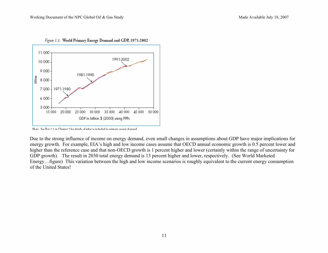
Income is the biggest determinant of demand for energy… Global and national incomes are the most significant determinant of energy demand. Long term price elasticities of demand are by some estimates as high as or higher than income elasticities of demand (in absolute values), but prices tend to go up and down (in real terms), whereas income historically increases year after year due to increases in population and per capita incomes. While the impact of energy price increases on energy demand are offset to some degree by energy price decreases, in normal times national and global incomes do not tend to move in reverse. Energy projections by the IEA and EIA are highly sensitive to GDP assumptions. In the WEO, one percent growth in global GDP results in a 0.5 percent increase in primary energy consumption. This is consistent with assumption reflects the observation that the income elasticity of demand fell from the 0.7 in the 1970s to 0.4 from 1991-2002 (see figure World Primary Energy…). WEO cites warmer winter weather in the northern hemisphere (which reduced heating fuel demand) and improved energy efficiency for the reduction in income elasticity for energy as a whole between the two periods (WEO 2006, p. 57). The income elasticities of demand for various energy resources vary, of course – e.g., the income elasticities of demand for electricity and transport fuels have remained constant (WEO says “linear”), though at a slower rate than, GDP since the 1970s (WEO 2006, p.58).
Working Document of the NPC Global Oil & Gas Study Made Available July 18, 2007
11
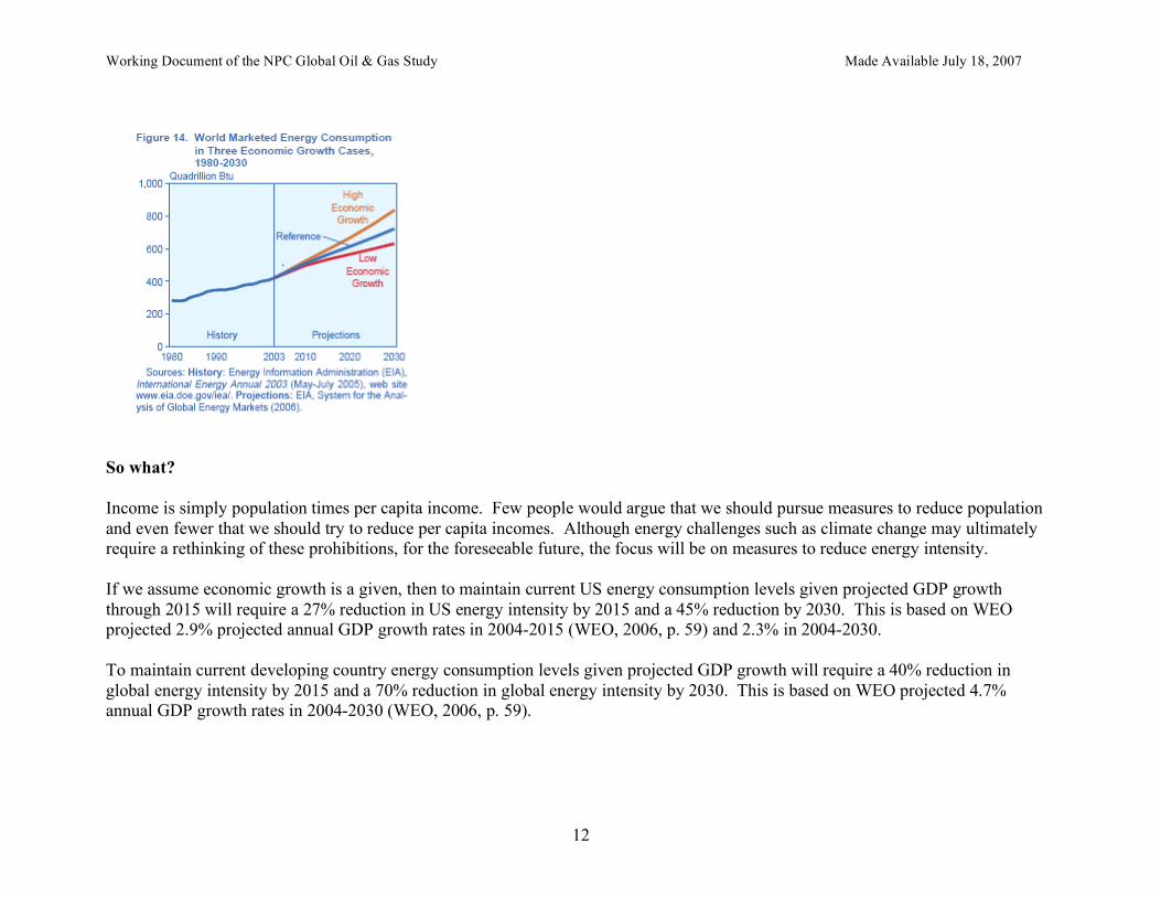
Due to the strong influence of income on energy demand, even small changes in assumptions about GDP have major implications for energy growth. For example, EIA’s high and low income cases assume that OECD annual economic growth is 0.5 percent lower and higher than the reference case and that non-OECD growth is 1 percent higher and lower (certainly within the range of uncertainty for GDP growth). The result in 2030 total energy demand is 13 percent higher and lower, respectively. (See World Marketed Energy…figure) This variation between the high and low income scenarios is roughly equivalent to the current energy consumption of the United States!
Working Document of the NPC Global Oil & Gas Study Made Available July 18, 2007
12
So what? Income is simply population times per capita income. Few people would argue that we should pursue measures to reduce population and even fewer that we should try to reduce per capita incomes. Although energy challenges such as climate change may ultimately require a rethinking of these prohibitions, for the foreseeable future, the focus will be on measures to reduce energy intensity. If we assume economic growth is a given, then to maintain current US energy consumption levels given projected GDP growth through 2015 will require a 27% reduction in US energy intensity by 2015 and a 45% reduction by 2030. This is based on WEO projected 2.9% projected annual GDP growth rates in 2004-2015 (WEO, 2006, p. 59) and 2.3% in 2004-2030. To maintain current developing country energy consumption levels given projected GDP growth will require a 40% reduction in global energy intensity by 2015 and a 70% reduction in global energy intensity by 2030. This is based on WEO projected 4.7% annual GDP growth rates in 2004-2030 (WEO, 2006, p. 59).
Working Document of the NPC Global Oil & Gas Study Made Available July 18, 2007
13
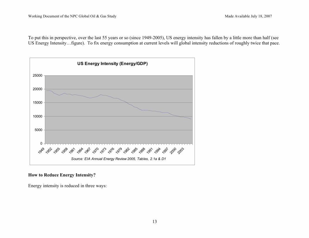
To put this in perspective, over the last 55 years or so (since 1949-2005), US energy intensity has fallen by a little more than half (see US Energy Intensity…figure). To fix energy consumption at current levels will global intensity reductions of roughly twice that pace.
US Energy Intensity (Energy/GDP)
0
5000
10000
15000
20000
25000
1949
1952
1955
1958
1961
1964
1967
1970
1973
1976
1979
1982
1985
1988
1991
1994
1997
2000
2003
Source: EIA Annual Energy Review 2005, Tables, 2.1a & D1
How to Reduce Energy Intensity? Energy intensity is reduced in three ways:
Working Document of the NPC Global Oil & Gas Study Made Available July 18, 2007
14
1) Structural changes in the economy – reduced share of energy-intensive activities in the economy. For example, as services have taken a larger share of the national and global economy (relative to heavy industry for example) the energy intensity of the national and global economies has fallen. Note that this does not mean that the amount of heavy industry has declined in absolute terms, just that the share of heavy industry has fallen and the share of less energy intensive industry has increased. 2) Energy efficiency – reduced energy per unit of energy services provided. Energy efficiency can be increased through technological improvement embedded in hardware (increased copper windings in electric motors, electronic lighting ballasts, electronic controls in buildings and vehicles, aerodynamic designs and lightweight materials for vehicles, etc). Alternatively, operations and management practices can be improved (e.g., building commissioning practices, replacement of air filters, adjusting tire pressures, etc.). 3) Energy conservation -- reduced demand for energy services as a share of total global consumption of products and services. For example, we can reduce vehicle miles traveled, horsepower and weight for vehicles. Similarly, we can reduce the size, plug loads and air conditioning in homes.1
Reductions in energy intensity are occurring naturally, without government interventions. As noted above, the energy intensity of the US economy is half what it was a few decades ago. Energy intensity reductions will continue, driven by increased energy efficiency and continued growth in the share of services in the global economy. On a national level, structural changes can be induced to reduce energy intensity. US policies could encourage heavy industry to move abroad, for example. If the policy objective is energy security, this could be advantageous, assuming, of course, that energy dependence isn’t replaced with similar dependence on the product of the heavy industry, which could even be more problematic. If the objective is to reduce global energy use -- e.g., to address global (as opposed to local) resource depletion concerns or reduce energy-related carbon emissions -- a policy to move heavy industry offshore could have deleterious impacts – for example, if the offshore factory is less efficient than the on shore factory it replaces.
1 The distinction between conservation and energy efficiency is not always clear– for example, depending on how you look at it, turning off lights when not in the room could be considered efficiency or conservation. Certainly if you turn lights off when you’re in the room and trying to read, that would be conservation. But turning lights off when you leave the room – and there is no reduction in energy services such as security – is more efficient.
Working Document of the NPC Global Oil & Gas Study Made Available July 18, 2007
15
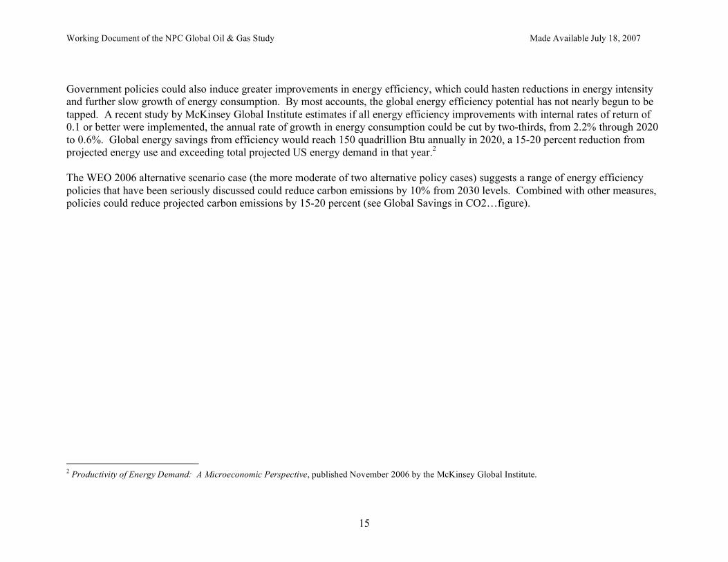
Government policies could also induce greater improvements in energy efficiency, which could hasten reductions in energy intensity and further slow growth of energy consumption. By most accounts, the global energy efficiency potential has not nearly begun to be tapped. A recent study by McKinsey Global Institute estimates if all energy efficiency improvements with internal rates of return of 0.1 or better were implemented, the annual rate of growth in energy consumption could be cut by two-thirds, from 2.2% through 2020 to 0.6%. Global energy savings from efficiency would reach 150 quadrillion Btu annually in 2020, a 15-20 percent reduction from projected energy use and exceeding total projected US energy demand in that year.2 The WEO 2006 alternative scenario case (the more moderate of two alternative policy cases) suggests a range of energy efficiency policies that have been seriously discussed could reduce carbon emissions by 10% from 2030 levels. Combined with other measures, policies could reduce projected carbon emissions by 15-20 percent (see Global Savings in CO2…figure).
2 Productivity of Energy Demand: A Microeconomic Perspective, published November 2006 by the McKinsey Global Institute.
Working Document of the NPC Global Oil & Gas Study Made Available July 18, 2007
16
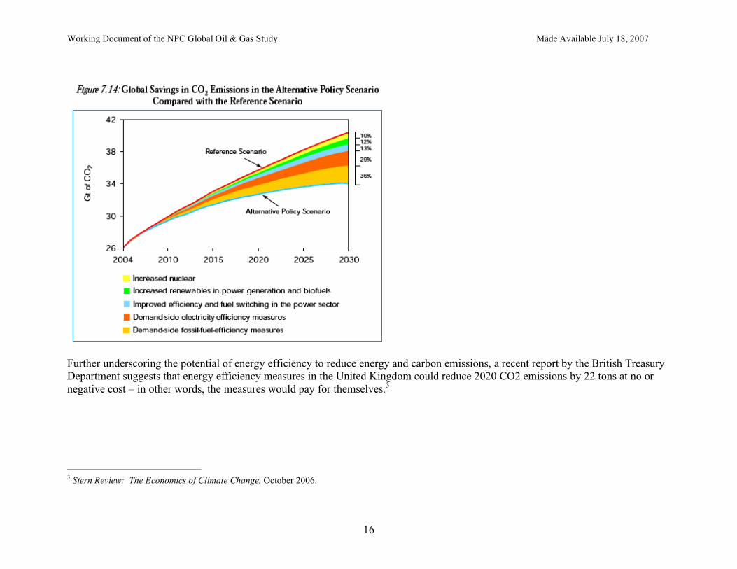
Further underscoring the potential of energy efficiency to reduce energy and carbon emissions, a recent report by the British Treasury Department suggests that energy efficiency measures in the United Kingdom could reduce 2020 CO2 emissions by 22 tons at no or negative cost – in other words, the measures would pay for themselves.3 3 Stern Review: The Economics of Climate Change, October 2006.
Working Document of the NPC Global Oil & Gas Study Made Available July 18, 2007
17
Importantly, the efficiency potential suggested by these studies will not be realized without significant government interventions. For example, businesses and consumers have shown over and again their unwillingness to make investments with returns of 10% – 2-year paybacks for businesses are often cited as the minimum for energy efficiency investments and consumers often make decisions that imply returns of 50% or more. Lack of awareness and know-how are two additional examples of barriers to investments in improved energy efficiency. And if history is our guide, without government interventions, energy intensity reductions resulting from improved efficiency and structural change will be largely offset by increased demand for energy services. For example, improvements in vehicle energy efficiency have been swamped by increases in vehicle horsepower and weight; likewise, improvements in the efficiency of appliances and buildings codes have been offset by increased number of appliances in homes and home size.
Working Document of the NPC Global Oil & Gas Study Made Available July 18, 2007
18
While policies to promote improved energy efficiency may be more politically palatable than policies to restrict demand for energy services, the former may not be sufficient if significant reductions from baseline in energy demand are required. Take Away Points
1. Income is the most important determinant of energy demand. 2. Income (= population x per capita income) is off limits. 3. Must target energy intensity instead -- i.e., structural change, energy efficiency, and demand for energy services. 4. Autonomous energy efficiency improvements and structural changes will have a large impact on energy intensity. 5. Government policy can induce additional energy efficiency improvements. 6. But growing demand for energy services will offset much of reductions in energy intensity resulting from efficiency and
structural change. 7. Government policy may also need to address growing demand for energy services
Working Document of the NPC Global Oil & Gas Study Made Available July 18, 2007
19
Oil and Gas Continue to Play a Large Role in Our Energy Future Leads: Joe Loper and Steve Capanna (Alliance to Save Energy)
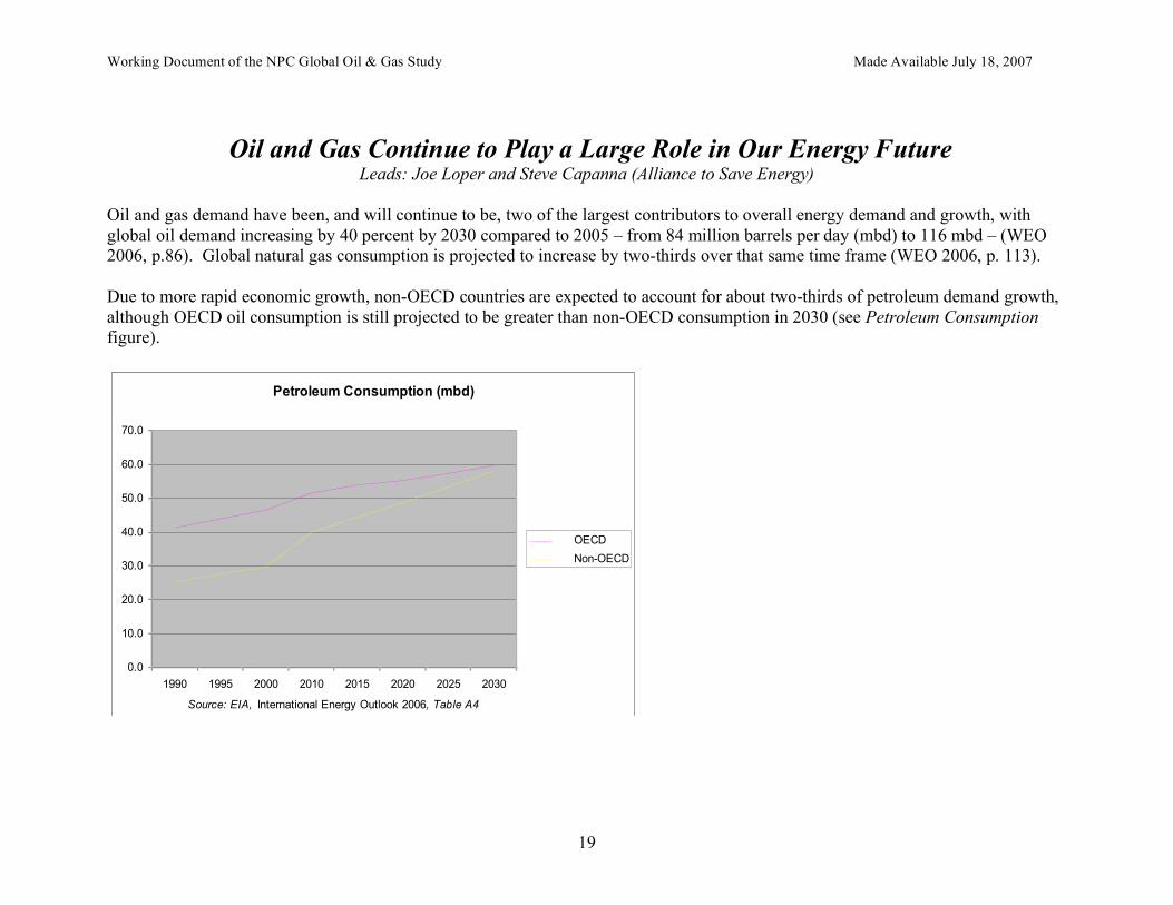
Oil and gas demand have been, and will continue to be, two of the largest contributors to overall energy demand and growth, with global oil demand increasing by 40 percent by 2030 compared to 2005 – from 84 million barrels per day (mbd) to 116 mbd – (WEO 2006, p.86). Global natural gas consumption is projected to increase by two-thirds over that same time frame (WEO 2006, p. 113). Due to more rapid economic growth, non-OECD countries are expected to account for about two-thirds of petroleum demand growth, although OECD oil consumption is still projected to be greater than non-OECD consumption in 2030 (see Petroleum Consumption figure).
Petroleum Consumption (mbd)
0.0
10.0
20.0
30.0
40.0
50.0
60.0
70.0
1990 1995 2000 2010 2015 2020 2025 2030
Source: EIA, International Energy Outlook 2006, Table A4
OECD
Non-OECD
Working Document of the NPC Global Oil & Gas Study Made Available July 18, 2007
20
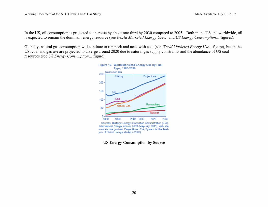
In the US, oil consumption is projected to increase by about one-third by 2030 compared to 2005. Both in the US and worldwide, oil is expected to remain the dominant energy resource (see World Marketed Energy Use… and US Energy Consumption… figures). Globally, natural gas consumption will continue to run neck and neck with coal (see World Marketed Energy Use…figure), but in the US, coal and gas use are projected to diverge around 2020 due to natural gas supply constraints and the abundance of US coal resources (see US Energy Consumption… figure).
US Energy Consumption by Source
Working Document of the NPC Global Oil & Gas Study Made Available July 18, 2007
21
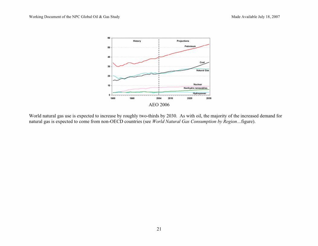
AEO 2006
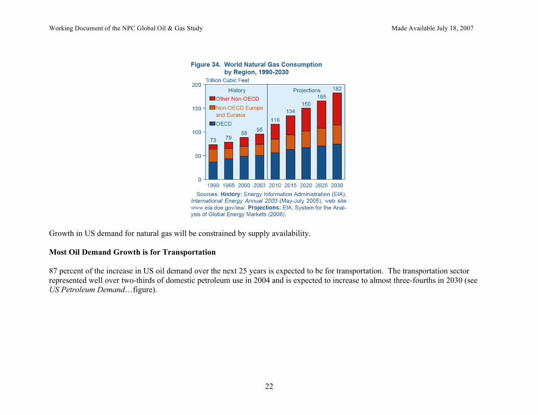
World natural gas use is expected to increase by roughly two-thirds by 2030. As with oil, the majority of the increased demand for natural gas is expected to come from non-OECD countries (see World Natural Gas Consumption by Region…figure).
Working Document of the NPC Global Oil & Gas Study Made Available July 18, 2007
22
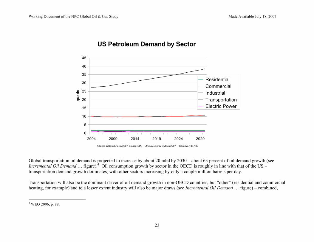
Growth in US demand for natural gas will be constrained by supply availability. Most Oil Demand Growth is for Transportation 87 percent of the increase in US oil demand over the next 25 years is expected to be for transportation. The transportation sector represented well over two-thirds of domestic petroleum use in 2004 and is expected to increase to almost three-fourths in 2030 (see US Petroleum Demand…figure).
Working Document of the NPC Global Oil & Gas Study Made Available July 18, 2007
23
US Petroleum Demand by Sector
0
5
10
15
20
25
30
35
40
45
2004 2009 2014 2019 2024 2029
Alliance to Save Energy 2007, Source: EIA, Annual Energy Outlook 2007 , Table A2, 138-139
qu
ad
s Residential
Commercial
Industrial
Transportation
Electric Power
Global transportation oil demand is projected to increase by about 20 mbd by 2030 – about 63 percent of oil demand growth (see Incremental Oil Demand … figure).4 Oil consumption growth by sector in the OECD is roughly in line with that of the US – transportation demand growth dominates, with other sectors increasing by only a couple million barrels per day. Transportation will also be the dominant driver of oil demand growth in non-OECD countries, but “other” (residential and commercial heating, for example) and to a lesser extent industry will also be major draws (see Incremental Oil Demand … figure) – combined,
4 WEO 2006, p. 88.
Working Document of the NPC Global Oil & Gas Study Made Available July 18, 2007
24
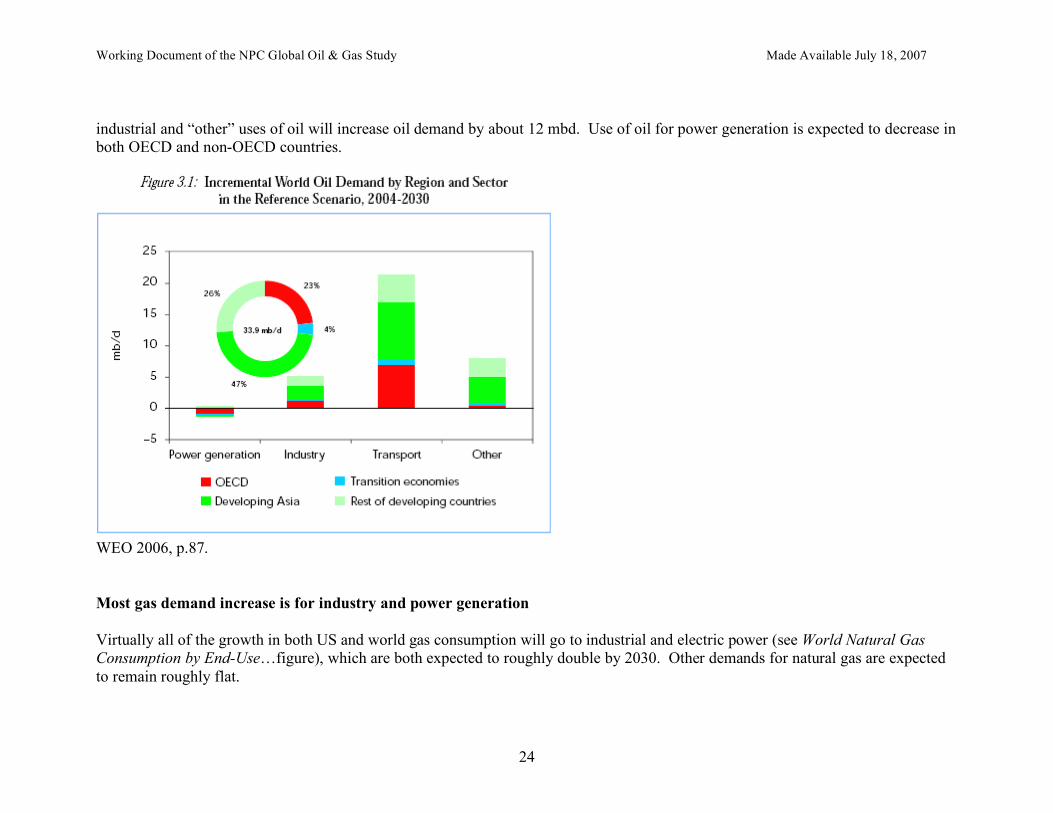
industrial and “other” uses of oil will increase oil demand by about 12 mbd. Use of oil for power generation is expected to decrease in both OECD and non-OECD countries.
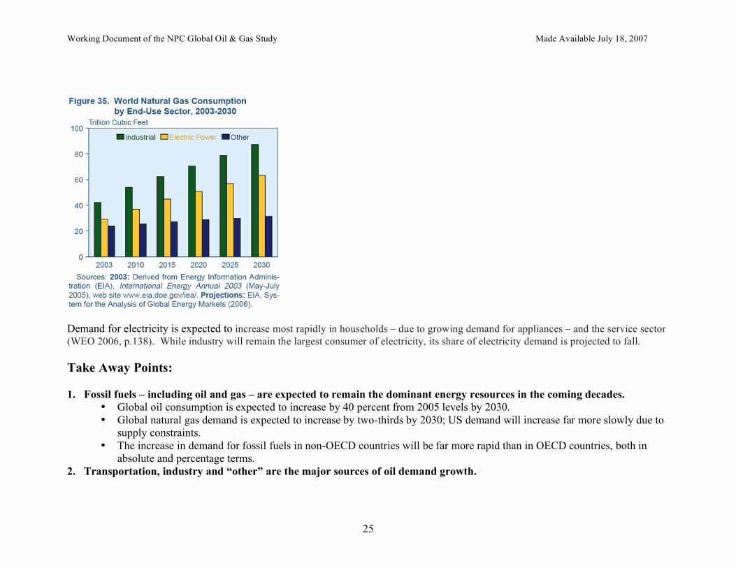
WEO 2006, p.87. Most gas demand increase is for industry and power generation Virtually all of the growth in both US and world gas consumption will go to industrial and electric power (see World Natural Gas Consumption by End-Use…figure), which are both expected to roughly double by 2030. Other demands for natural gas are expected to remain roughly flat.
Working Document of the NPC Global Oil & Gas Study Made Available July 18, 2007
25
Demand for electricity is expected to increase most rapidly in households – due to growing demand for appliances – and the service sector (WEO 2006, p.138). While industry will remain the largest consumer of electricity, its share of electricity demand is projected to fall. Take Away Points: 1. Fossil fuels – including oil and gas – are expected to remain the dominant energy resources in the coming decades.
• Global oil consumption is expected to increase by 40 percent from 2005 levels by 2030. • Global natural gas demand is expected to increase by two-thirds by 2030; US demand will increase far more slowly due to
supply constraints. • The increase in demand for fossil fuels in non-OECD countries will be far more rapid than in OECD countries, both in
absolute and percentage terms. 2. Transportation, industry and “other” are the major sources of oil demand growth.
Working Document of the NPC Global Oil & Gas Study Made Available July 18, 2007
26
• Oil demand growth in the transportation sector will exceed growth for all other uses combined. • But projected industry and “other” category oil consumption are expected to increase by a large amount: 13 mbd.
3. Electric power generation and industry are the major sources of natural gas demand growth. • Natural gas demand for electric generation and industry are expected to double. • Other uses of natural gas are expected to remain roughly flat.
4. Less obvious, energy use in buildings will be a major source of oil and gas demand growth. • Appliances and other “buildings” related energy uses represent the largest electricity demand growth, and thus having
major impact on the demand for natural gas. • “Other” (including building heating) is a major source of oil demand growth.
Working Document of the NPC Global Oil & Gas Study Made Available July 18, 2007
27
Light Duty Vehicle Trends Leads: Deron Lovaas (Natural Resources Defense Council)
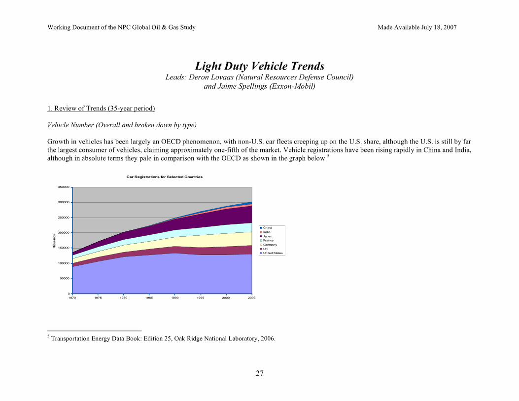
and Jaime Spellings (Exxon-Mobil) 1. Review of Trends (35-year period) Vehicle Number (Overall and broken down by type) Growth in vehicles has been largely an OECD phenomenon, with non-U.S. car fleets creeping up on the U.S. share, although the U.S. is still by far the largest consumer of vehicles, claiming approximately one-fifth of the market. Vehicle registrations have been rising rapidly in China and India, although in absolute terms they pale in comparison with the OECD as shown in the graph below.5
Car Registrations for Selected Countries
0
50000
100000
150000
200000
250000
300000
350000
1970 1975 1980 1985 1990 1995 2000 2003
thou
sand
s
China
India
Japan
France
Germany
UK
United States
5 Transportation Energy Data Book: Edition 25, Oak Ridge National Laboratory, 2006.
Working Document of the NPC Global Oil & Gas Study Made Available July 18, 2007
28
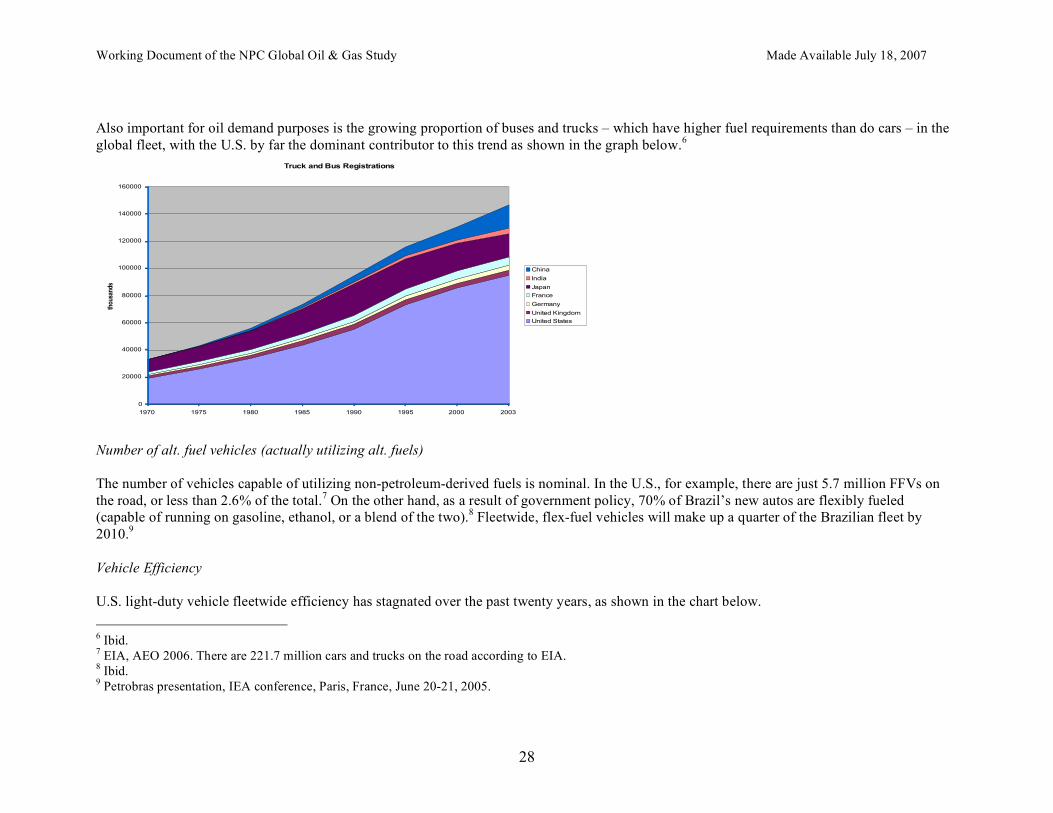
Also important for oil demand purposes is the growing proportion of buses and trucks – which have higher fuel requirements than do cars – in the global fleet, with the U.S. by far the dominant contributor to this trend as shown in the graph below.6
Truck and Bus Registrations
0
20000
40000
60000
80000
100000
120000
140000
160000
1970 1975 1980 1985 1990 1995 2000 2003
thou
sand
s
China
India
Japan
France
Germany
United Kingdom
United States
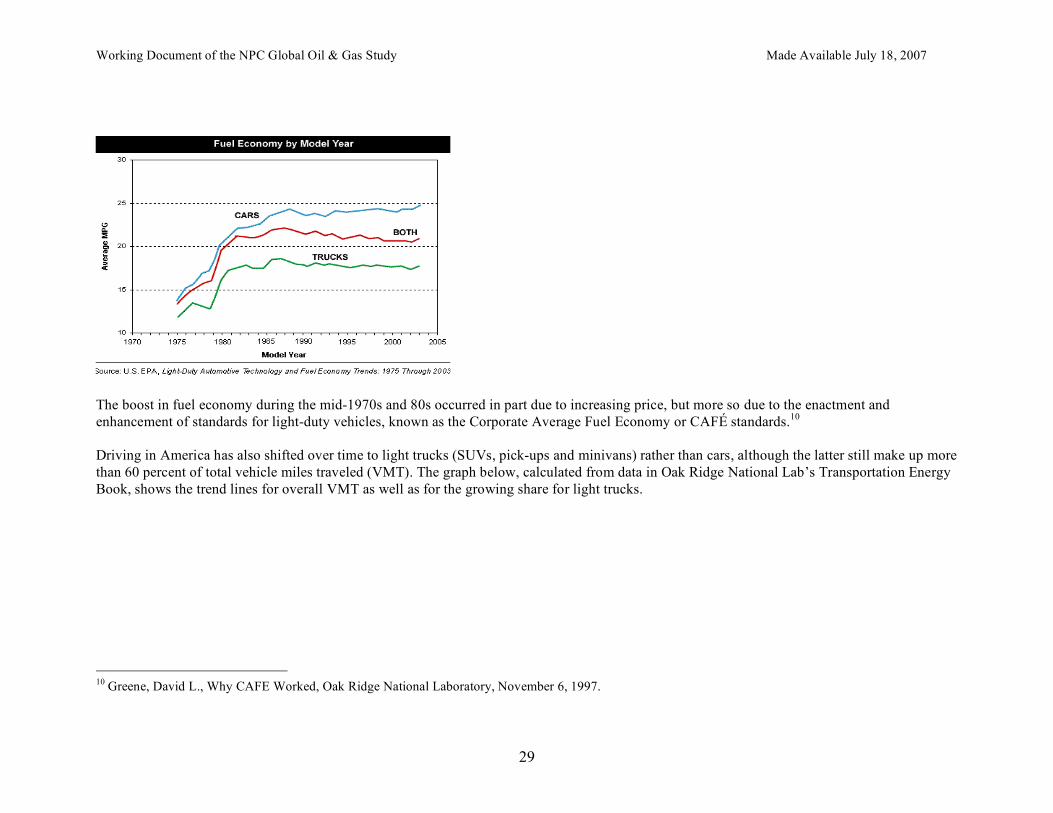
Number of alt. fuel vehicles (actually utilizing alt. fuels) The number of vehicles capable of utilizing non-petroleum-derived fuels is nominal. In the U.S., for example, there are just 5.7 million FFVs on the road, or less than 2.6% of the total.7 On the other hand, as a result of government policy, 70% of Brazil’s new autos are flexibly fueled (capable of running on gasoline, ethanol, or a blend of the two).8 Fleetwide, flex-fuel vehicles will make up a quarter of the Brazilian fleet by 2010.9 Vehicle Efficiency U.S. light-duty vehicle fleetwide efficiency has stagnated over the past twenty years, as shown in the chart below. 6 Ibid. 7 EIA, AEO 2006. There are 221.7 million cars and trucks on the road according to EIA. 8 Ibid. 9 Petrobras presentation, IEA conference, Paris, France, June 20-21, 2005.
Working Document of the NPC Global Oil & Gas Study Made Available July 18, 2007
29
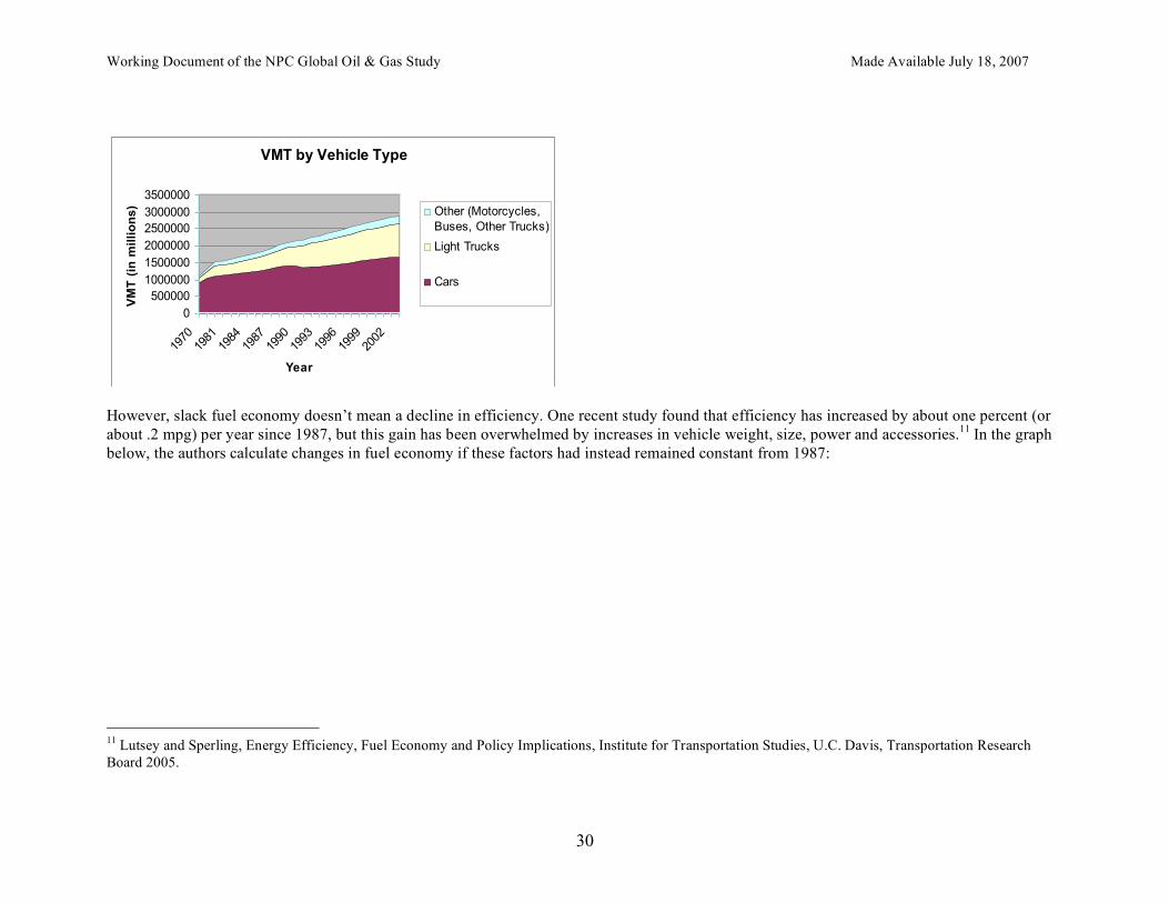
The boost in fuel economy during the mid-1970s and 80s occurred in part due to increasing price, but more so due to the enactment and enhancement of standards for light-duty vehicles, known as the Corporate Average Fuel Economy or CAFÉ standards.10 Driving in America has also shifted over time to light trucks (SUVs, pick-ups and minivans) rather than cars, although the latter still make up more than 60 percent of total vehicle miles traveled (VMT). The graph below, calculated from data in Oak Ridge National Lab’s Transportation Energy Book, shows the trend lines for overall VMT as well as for the growing share for light trucks.
10 Greene, David L., Why CAFE Worked, Oak Ridge National Laboratory, November 6, 1997.
Working Document of the NPC Global Oil & Gas Study Made Available July 18, 2007
30
VMT by Vehicle Type
0
500000
1000000
1500000
2000000
2500000
3000000
3500000
1970
1981
1984
1987
1990
1993
1996
1999
2002
Year
VM
T (
in m
illi
on
s) Other (Motorcycles,
Buses, Other Trucks)
Light Trucks
Cars
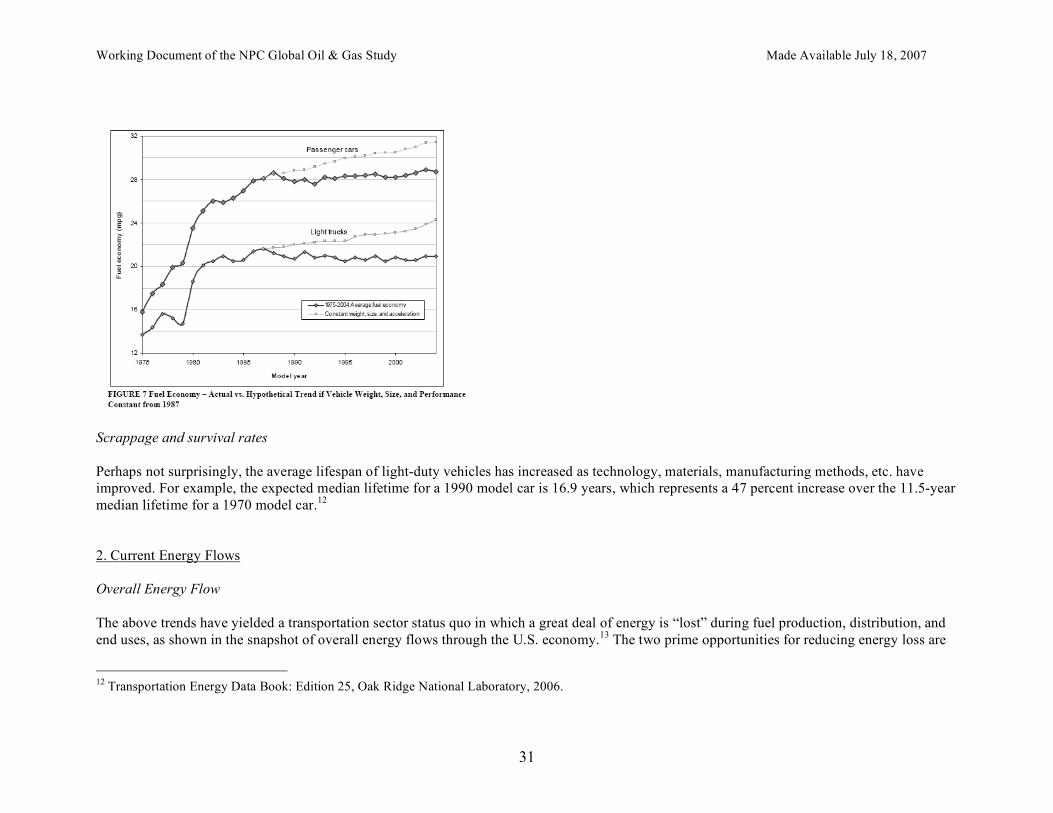
However, slack fuel economy doesn’t mean a decline in efficiency. One recent study found that efficiency has increased by about one percent (or about .2 mpg) per year since 1987, but this gain has been overwhelmed by increases in vehicle weight, size, power and accessories.11 In the graph below, the authors calculate changes in fuel economy if these factors had instead remained constant from 1987:
11 Lutsey and Sperling, Energy Efficiency, Fuel Economy and Policy Implications, Institute for Transportation Studies, U.C. Davis, Transportation Research Board 2005.
Working Document of the NPC Global Oil & Gas Study Made Available July 18, 2007
31
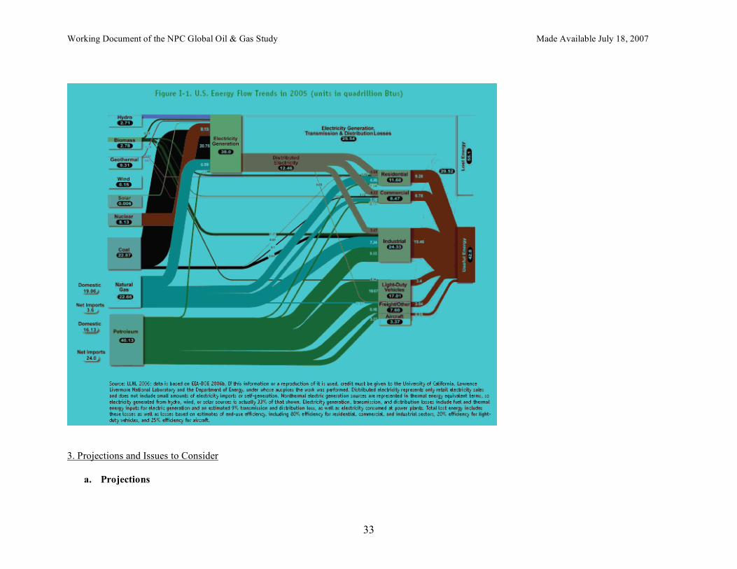
Scrappage and survival rates Perhaps not surprisingly, the average lifespan of light-duty vehicles has increased as technology, materials, manufacturing methods, etc. have improved. For example, the expected median lifetime for a 1990 model car is 16.9 years, which represents a 47 percent increase over the 11.5-year median lifetime for a 1970 model car.12 2. Current Energy Flows Overall Energy Flow The above trends have yielded a transportation sector status quo in which a great deal of energy is “lost” during fuel production, distribution, and end uses, as shown in the snapshot of overall energy flows through the U.S. economy.13 The two prime opportunities for reducing energy loss are
12 Transportation Energy Data Book: Edition 25, Oak Ridge National Laboratory, 2006.

Working Document of the NPC Global Oil & Gas Study Made Available July 18, 2007
32
clearly illustrated by this graph: 1) electricity generation, where 67 percent of energy is lost, and 2) transportation end uses, where 76% percent of energy is lost (80% from light-duty vehicles alone).
13 Created by the University of California, Lawrence Livermore National Laboratory and DOE for the President’s Council of Advisors on Science and Technology based on 2006 EIA data.
Working Document of the NPC Global Oil & Gas Study Made Available July 18, 2007
33
3. Projections and Issues to Consider
a. Projections
Working Document of the NPC Global Oil & Gas Study Made Available July 18, 2007
34
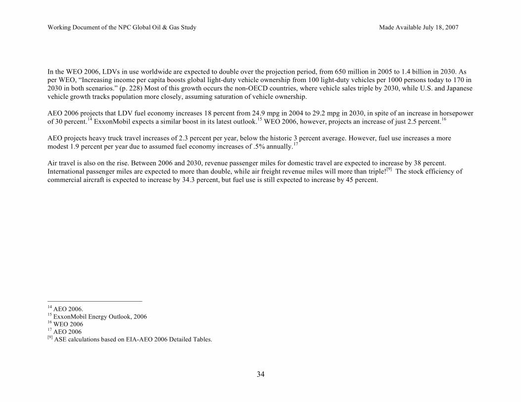
In the WEO 2006, LDVs in use worldwide are expected to double over the projection period, from 650 million in 2005 to 1.4 billion in 2030. As per WEO, “Increasing income per capita boosts global light-duty vehicle ownership from 100 light-duty vehicles per 1000 persons today to 170 in 2030 in both scenarios.” (p. 228) Most of this growth occurs the non-OECD countries, where vehicle sales triple by 2030, while U.S. and Japanese vehicle growth tracks population more closely, assuming saturation of vehicle ownership. AEO 2006 projects that LDV fuel economy increases 18 percent from 24.9 mpg in 2004 to 29.2 mpg in 2030, in spite of an increase in horsepower of 30 percent.14 ExxonMobil expects a similar boost in its latest outlook.15 WEO 2006, however, projects an increase of just 2.5 percent.16 AEO projects heavy truck travel increases of 2.3 percent per year, below the historic 3 percent average. However, fuel use increases a more modest 1.9 percent per year due to assumed fuel economy increases of .5% annually.17 Air travel is also on the rise. Between 2006 and 2030, revenue passenger miles for domestic travel are expected to increase by 38 percent. International passenger miles are expected to more than double, while air freight revenue miles will more than triple![9] The stock efficiency of commercial aircraft is expected to increase by 34.3 percent, but fuel use is still expected to increase by 45 percent.
14 AEO 2006. 15 ExxonMobil Energy Outlook, 2006 16 WEO 2006 17 AEO 2006 [9] ASE calculations based on EIA-AEO 2006 Detailed Tables.
Working Document of the NPC Global Oil & Gas Study Made Available July 18, 2007
35
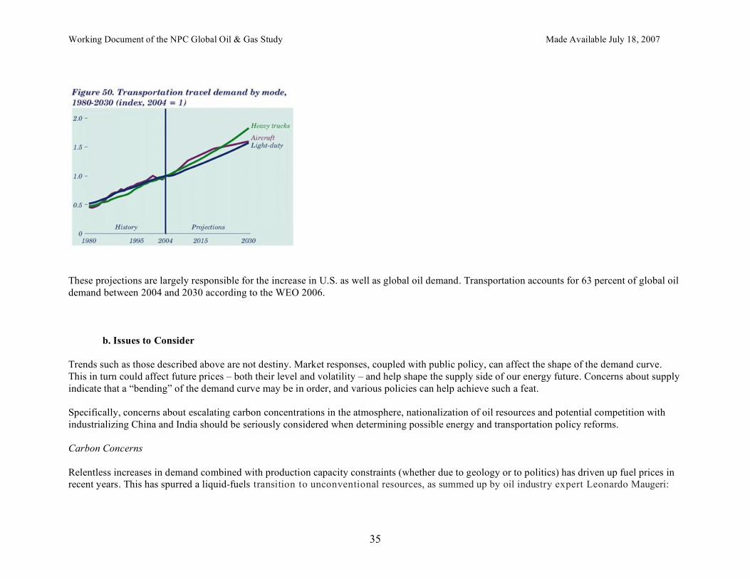
These projections are largely responsible for the increase in U.S. as well as global oil demand. Transportation accounts for 63 percent of global oil demand between 2004 and 2030 according to the WEO 2006. b. Issues to Consider Trends such as those described above are not destiny. Market responses, coupled with public policy, can affect the shape of the demand curve. This in turn could affect future prices – both their level and volatility – and help shape the supply side of our energy future. Concerns about supply indicate that a “bending” of the demand curve may be in order, and various policies can help achieve such a feat. Specifically, concerns about escalating carbon concentrations in the atmosphere, nationalization of oil resources and potential competition with industrializing China and India should be seriously considered when determining possible energy and transportation policy reforms. Carbon Concerns Relentless increases in demand combined with production capacity constraints (whether due to geology or to politics) has driven up fuel prices in recent years. This has spurred a liquid-fuels transition to unconventional resources, as summed up by oil industry expert Leonardo Maugeri:
Working Document of the NPC Global Oil & Gas Study Made Available July 18, 2007
36
Indeed, a process of “deconventionalization” of reserves is taking place that will probably make the future supply of oil the result of a mosaic of many increments, many of them relatively small, coming from both new and traditional producing countries, and from unconventional sources such as gas liquids, ultra-deep offshore deposits, ultra-heavy oils, shale oils, and tar sands.18
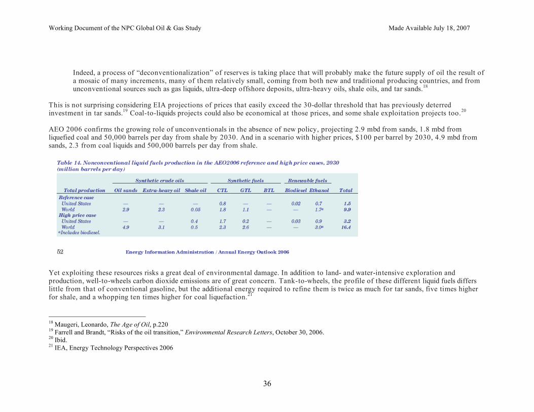
This is not surprising considering EIA projections of prices that easily exceed the 30-dollar threshold that has previously deterred investment in tar sands.19 Coal-to-liquids projects could also be economical at those prices, and some shale exploitation projects too.20 AEO 2006 confirms the growing role of unconventionals in the absence of new policy, projecting 2.9 mbd from sands, 1.8 mbd from liquefied coal and 50,000 barrels per day from shale by 2030. And in a scenario with higher prices, $100 per barrel by 2030, 4.9 mbd from sands, 2.3 from coal liquids and 500,000 barrels per day from shale.
Yet exploiting these resources risks a great deal of environmental damage. In addition to land- and water-intensive exploration and production, well-to-wheels carbon dioxide emissions are of great concern. Tank-to-wheels, the profile of these different liquid fuels differs little from that of conventional gasoline, but the additional energy required to refine them is twice as much for tar sands, five times higher for shale, and a whopping ten times higher for coal liquefaction.21 18 Maugeri, Leonardo, The Age of Oil, p.220 19 Farrell and Brandt, “Risks of the oil transition,” Environmental Research Letters, October 30, 2006. 20 Ibid. 21 IEA, Energy Technology Perspectives 2006
Working Document of the NPC Global Oil & Gas Study Made Available July 18, 2007
37
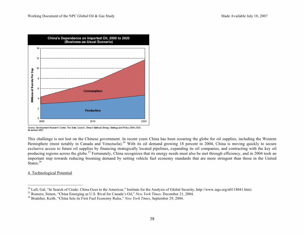
Energy Security Concerns Many have expressed concern about the re-ascendance of the national oil companies, especially those where geopolitical or ideological agendas may trump commercial ones (i.e., Iran, Venezuela, and sadly perhaps Iraq someday). Others have concern about the growth of China, which is forging deals with countries far afield, including in the Western Hemisphere (i.e., Venezuela). While per capita petroleum consumption is just six percent of the U.S. figure, rapid industrialization and a growing consumer culture mean China’s demand for imported oil is projected to grow from less than 2 million barrels per day in 2004 to nearly 8 million barrels per day by 2020 (see graph below).22 While U.S. import dependence will rise to nearly 70 percent by 2025, India already imports 70 percent of its oil and the import share in China is expected to grow from 40 to 75 percent over the same time period.23 Business as usual keeps the United States on a path fraught with increasingly tight competition with other oil-needy nations.
22 International Energy Agency cited by Interfax, “Foreign Investment to Play Key Role in Development of China’s Oil and Gas,” China Weekly Energy Report, May 22-28, 2004. 23 Manjeet Kripalani, Dexter Roberts, Jason Bush. India And China: Oil-Patch Partners? Businessweek, February 7, 2005.
Working Document of the NPC Global Oil & Gas Study Made Available July 18, 2007
38
This challenge is not lost on the Chinese government. In recent years China has been scouring the globe for oil supplies, including the Western Hemisphere (most notably in Canada and Venezuela).24 With its oil demand growing 18 percent in 2004, China is moving quickly to secure exclusive access to future oil supplies by financing strategically located pipelines, expanding its oil companies, and contracting with the key oil producing regions across the globe.25 Fortunately, China recognizes that its energy needs must also be met through efficiency, and in 2004 took an important step towards reducing booming demand by setting vehicle fuel economy standards that are more stringent than those in the United States.26 4. Technological Potential
24 Luft, Gal, “In Search of Crude: China Goes to the Americas,” Institute for the Analysis of Global Security, http://www.iags.org/n0118041.htm) 25 Romero, Simon, “China Emerging as U.S. Rival for Canada’s Oil,” New York Times, December 21, 2004. 26 Bradsher, Keith, “China Sets its First Fuel Economy Rules,” New York Times, September 29, 2004.
Working Document of the NPC Global Oil & Gas Study Made Available July 18, 2007
39
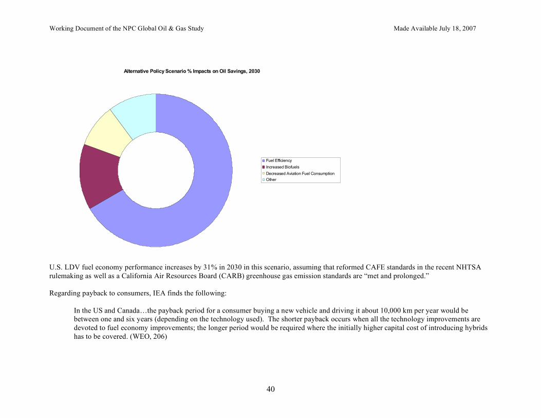
Conventional Technology There are several technologies that could be utilized without shortchanging vehicle performance, including continuously variable transmission, engine supercharging and turbocharging, variable valve timing, cylinder deactivation, aerodynamic design, integrated starter/generator, and low-resistance tires. In fact, in its 2002 report on fuel economy standards, the National Research Council (2002) found that a combination of various technologies could boost LDV fuel economy performance by one-third.27 Spurred by increased demand for fuel economy in the marketplace, engineers continue to develop new techniques for boosting efficiency. For example, MIT is working with Ford on engine modifications which use an ethanol mist sprayed directly into hot cylinders, boosting performance by an impressive 30% at the cost of $1,000 per vehicle.28 Advanced Technology In its WEO 2006 Alternative Policy Scenario, IEA also looks to increases in efficiency using conventional technology coupled with advanced technology. In order to save 7.6 mbd while addressing both energy security and climate concerns, IEA assumes improvements such that 60% of new LDV sales are “mild hybrids” and 18% are “full hybrids,” that biofuels makes up 7% of the liquid fuel mix as opposed to 4% in the reference case, and that aviation oil consumption drops 7% due to increased efficiency and a modal shift to high-speed rail. The graph below shows the necessary, if insufficient, role that vehicle efficiency gains play in this scenario.
27 Effectiveness and Impact of Corporate Average Fuel Economy (CAFE) Standards (2002), National Research Council, NAS 28 “Developments to Watch,” BusinessWeek, November 20, 2006.
Working Document of the NPC Global Oil & Gas Study Made Available July 18, 2007
40
Alternative Policy Scenario % Impacts on Oil Savings, 2030
Fuel Efficiency
Increased Biofuels
Decreased Aviation Fuel Consumption
Other
U.S. LDV fuel economy performance increases by 31% in 2030 in this scenario, assuming that reformed CAFE standards in the recent NHTSA rulemaking as well as a California Air Resources Board (CARB) greenhouse gas emission standards are “met and prolonged.” Regarding payback to consumers, IEA finds the following:
In the US and Canada…the payback period for a consumer buying a new vehicle and driving it about 10,000 km per year would be between one and six years (depending on the technology used). The shorter payback occurs when all the technology improvements are devoted to fuel economy improvements; the longer period would be required where the initially higher capital cost of introducing hybrids has to be covered. (WEO, 206)
Working Document of the NPC Global Oil & Gas Study Made Available July 18, 2007
41
IEA recognizes, however, that even its Alternative Policy Scenario falls short of shoring up either energy security or climate goals by leaving the world 77% dependent on fossil fuels and emitting an additional 8 gigatons of heat-trapping CO2. The transportation sector plays a substantial role in a more aggressive scenario in which CO2 emissions level off at their 2004 levels. The IEA specifically includes under its Beyond the Alternative Policy Scenario (BAPS) increasing “full hybrid” penetration to 60% (instead of 18%), promoting plug-in hybrids in the marketplace, and doubling the use of biofuels by 2030. By 2030, this would save 14.6 mbd, as opposed to 7 mbd saved in the Alternative Policy Scenario. Policy Options In evaluating policy options related to transportation, one must begin with a clear understanding of the problem to be solved. Today, there are several candidate problems: high prices, volatile prices, energy security, energy dependency, air pollution (or health impacts) and global warming. The request for this study arose out of a concern that supply for oil and gas may not be available to meet growing demand. This concern encompasses both today's high prices and volatile prices. In addition, there is a related concern that supplies of oil and gas crucial to meeting current and growing future world demand are found in unstable or unfriendly countries. Dependence on exports from these countries creates unease. In addition, there is a completely separate concern about the need to restrain carbon emissions in order to reduce the risk of harmful climate change. Listed below are policy options for petroleum demand reduction. Fuel Economy Standards The Corporate Average Fuel Economy (CAFE) standard was enacted in 1975 in response to the first oil shocks and set separate standards for passenger cars and light trucks, including sport utility vehicles (SUVs) and minivans. The standards, combined with significant fuel price increases, led to a near doubling of fuel economy for passenger cars and a 50 percent increase for light trucks (NRC 2002, 14). Without CAFE standards, the U.S. would have used about 2.8 million barrels a day more gasoline in 2000 (NRDC 2002, 20). Average fuel economy for the combined fleet peaked in 1988 at 22.1 mpg and has declined since then due to two main reasons. First, the passenger car fleet standards have not been increased since 1990 and remain at 27.5 mpg. Second, the share of light duty trucks has increased to ~50% of new vehicle sales due to the rise in popularity of SUVs and minivans. Because this category was originally dominated by “work trucks” (pickups) and these vehicles tend to be heavier and less aerodynamic than cars, they have been held to a lower fuel economy standard. The significant shift in consumer vehicle buying patterns and the lack of
Working Document of the NPC Global Oil & Gas Study Made Available July 18, 2007
42
policy response have significantly eroded the effectiveness of the CAFE standards. This illustrates a problem in writing any class-based standards without a requirement for aggregate improvement – something that a bipartisan group of Senators recently proposed -- and the need to move towards a standard that doesn’t encourage shifting among control categories. In 2003, the Bush administration revised the rules as applicable to light trucks and SUVs. In doing so, they created a new attribute-based standard system that allows manufacturers to have different CAFE standards depending on the sales-weighted mix of their vehicle fleet’s “footprint” (i.e., width times wheelbase). This has the advantage of avoiding one of the original critiques of CAFE--that it led automakers to reduce car size, which in turn made the cars less safe. A National Academies report on CAFE found that, although there were many complex issues involved, reducing vehicle weight did tend to make cars less safe, although there was a dissenting opinion written by two of the members because they believed the data confounded the issue of whether size or weight was the key factor. An idea to reduce the cost of compliance with higher CAFE standards is to establish a trading system for CAFE credits. In this system a manufacturer that was able to increase their fleet's performance at low cost could generate credits to be sold to other manufacturers whose cost of improvement was higher. The CBO estimated that a trading system could reduce the overall economic cost of a moderate (3.8 MPG) increase in CAFE by 16%. In considering the effectiveness of CAFE as a policy, one must as always be clear about the objective. CAFE, or any system of vehicle standards, requires automakers to manufacture products that must meet certain minimum standards, thereby affecting the fuel economy levels of vehicles that consumers are allowed to buy. As such, it can and does directly change the result that an otherwise free market would produce and raises the efficiency of new vehicles. Economic theory maintains that in the case of “externalities” where the full cost of using a product is not included in the private cost, it can be appropriate for government to intervene in the marketplace. Remediation of global warming and national security concerns related to petroleum use are all potential bases for government intervention in the market in order to improve overall societal welfare. Ideally, the costs of policy options for reducing fuel use should be weighed against the benefits, and that the most cost-effective policy be chosen to limit its impact on U.S. economic competitiveness. Another option to reduce gasoline use would be to raise the price by increasing fuel taxes, which might be justified as including the externality cost. Changes in CAFE policy, however, only affect new cars sold after the effective date and therefore take a long time to affect the overall fleet. In addition, by reducing the marginal cost of driving, an increase in CAFE could actually increase total vehicle miles traveled. While theory would say that consumers should be able to weigh the cost of more efficient vehicles against the future
Working Document of the NPC Global Oil & Gas Study Made Available July 18, 2007
43
fuel savings and make the optimal choice, some proponents of CAFE argue that consumers do not behave rationally in weighing current costs against future benefits. Recent evidence of elasticities suggests that affecting meaningful near-term reductions in petroleum use through prices alone would require extremely large increases in fuel prices. Transportation analysts have hypothesized that changing land-use patterns, increase in multiple income households and per capita disposable income, as well as decrease in the availability of the non-auto modes of transportation over the last thirty years has made the US consumer’s response to gasoline prices almost inelastic.29 A thoughtful review of policies should consider how standards and fuel prices might work together in a mutually complementary manner to ensure public policy goals are met. Fuel Taxes Some have proposed higher gasoline taxes as a way to reduce our dependence on oil. Current nationwide gasoline taxes total 46.8 cents per gallon and are comprised of an 18.4 cent per gallon federal excise tax used to support mass transit and highway programs and various state and local taxes. Gasoline taxes have declined about 13 percent since 1995 on an inflation-adjusted basis (2006 cents, source: API). If dependence on oil is the problem then higher taxes will (all other things being equal) discourage demand. Unlike CAFE regulations, a tax increase would be less of a direct intervention in the vehicle and fuels marketplace as consumers would theoretically be free to choose to either drive less or to purchase more fuel efficient vehicles or shift spending from other expenses to fuels. However, as stated above this is true only insofar as consumers actually have options -- in the near-term, some consumers will realistically not. This is one reason some experts have proposed a combination of higher standards and higher fuel taxes, and this would also argue for increased investment in alternatives to driving such as public transit. Key considerations in the development of a tax policy are public and political resistance to increasing taxes, addressing the disproportionate impact on low income consumers and equitably redistributing the additional government revenue generated by the tax. Assuming a large enough tax to overcome low elasticities yet designed to address inequitable distributional effects, some studies show that the near term impact on demand would be larger for a tax increase than for a change in CAFE standards as the former would impact all vehicles immediately while the latter only impacts new vehicles entering the fleet. A 2004 CBO study that considered both CAFE and tax policies that achieved the same long term reduction in fuel consumption concluded that the near-term fuel savings
29 J. E. Hughes, C. R. Knittel, D. Sperling, ITS Publication 06-16, U. of California, Davis, 2006.
Working Document of the NPC Global Oil & Gas Study Made Available July 18, 2007
44
would be 42% greater under the tax approach. If higher taxes resulted in a reduction in vehicle miles traveled, then additional benefits might be realized through reductions in congestion and vehicle accidents. Because both a gasoline tax and CAFE standards can result in reduced fuel consumption, an analysis of the options needs to consider the interaction between the two. For example, some analysts have proposed that higher CAFE standards could be justified if the gasoline tax was first increased, since internalizing costs of driving (pollution, congestion, and fatalities) would increase consumer support for higher standards. However, some claim that this approach fails to account for the cumulative costs of the two policies. Ethanol Ethanol as a component of transportation fuel directionally reduces petroleum consumption and increases natural gas use; however its impact is limited because the scale of corn-based ethanol is limited. Current federal law provides an excise tax credit for the blending of ethanol into gasoline of 51 cents per gallon of ethanol used as well as a CAFE credit for flex-fuel vehicles (those capable of running on 85% ethanol / 15% gasoline blend). Currently ethanol can be used either as E10 (up to 10% by volume) or as E85 (85% by volume). E10 is compatible with almost all cars on the road today as well as with existing fueling infrastructure. It does, however, incur additional distribution costs as the ethanol must remain segregated from gasoline in the distribution system in order avoid contamination from water. Use of ethanol as E10 shows increased emissions of volatile organic compounds and nitrogen oxides, and decreased in carbon monoxide emissions; however these emissions changes are small compared to changes in vehicle emissions standards. E85 on the other hand is a fundamentally different fuel that requires significant changes to the distribution and retailing fueling infrastructure as well as vehicles designed specifically to run on the fuel. There is limited data to assess emissions from E85, however, we expect emissions from vehicles using E85 to be similar to conventional vehicles using E0 or E10. The price of E85 is usually higher than that of gasoline (especially on an energy content basis), reflecting the limited supply of ethanol and high demand for blending as E10. The cost of producing ethanol from corn is roughly equal to the cost of producing gasoline from oil when oil is $40-$60 per barrel. The high prices of ethanol over much of 2006 have driven a tremendous investment in increased capacity. However the current corn-based ethanol production in the United States is estimated to have an economic limit of about 12-15 billion gallons per year.
Working Document of the NPC Global Oil & Gas Study Made Available July 18, 2007
45
Cellulose provides a potential feedstock for ethanol production that could be substantially larger than corn in the US, however at present the technology does not exist to produce cellulosic ethanol competitively with corn ethanol. Also, the impact of large scale production of cellulosic ethanol on land use, water consumption, quality of water table, etc. are not known. There are significant academic, government and commercial research activities underway that are seeking breakthroughs that could lower the production cost. There are differing opinions about the need for additional policy support for E85 vehicles and fueling infrastructure. Currently, the CAFE rules provide an incentive for automakers to supply flex fuel vehicles, and a tax credit exists for installing E85 fueling infrastructure. Some maintain that E85 should be further promoted to minimize the air pollution impacts associated with E10 and to allow steady growth in the ethanol industry. Others observe that the US could use three times today's ethanol production as E10 in the current vehicle fleet, and that the market will respond as evidenced by the growing percentage of retail outlets with E85 capability. Feebates Feebates are an alternative policy measure that has been proposed as a way to increase the average fuel economy of the fleet without mandating increases in CAFE standards, or possibly in concert with CAFE standards to provide an incentive for consumer support. Under this system consumers who purchase a vehicle with higher than average fuel economy would receive a rebate while those who purchase a vehicle with lower than average fuel economy would pay a fee. A feebate system would preserve free market choice for both consumers and vehicle producers and if properly implemented the system could be revenue neutral. A feebate system could take many different forms. A 2005 study led by Oak Ridge National Labs concluded that a moderate feebate ($500 to $1000) could improve the average fuel economy of new vehicles by between 8 and ~50% versus a no policy case depending on the details of the program. In most cases the government expenditures associated with the programs were 300M$ or less. Pay-As-You-Drive Insurance and Other Proposals for Making Fixed Costs Variable Other policies would provide economic incentives for reduced driving, providing societal benefits in the form of reduced congestion, fatalities and pollution. For example, Oregon provides incentives and Texas authorizes companies to offer pay-per-mile auto insurance, and Progressive Insurance piloted such a program from 1998-2001. A 2005 analysis by Resources for the Future found that a national program could reduce gasoline demand by 9.1% and provide significantly higher societal benefits than a gasoline tax calibrated to achieve similar savings due in part to reduced driving by riskier drivers.

Working Document of the NPC Global Oil & Gas Study Made Available July 18, 2007
46
Other policies could similarly make variable costs of driving which are currently fixed, such as mileage-based registration, leasing and rental fees. Such programs could also work in tandem with an increase in CAFE standards, mitigating or eliminating the VMT “rebound effect.”
Working Document of the NPC Global Oil & Gas Study Made Available July 18, 2007
47
Carbon Emissions Growing as Fast as Energy Consumption Leads: Joe Loper and Steve Capanna (Alliance to Save Energy)
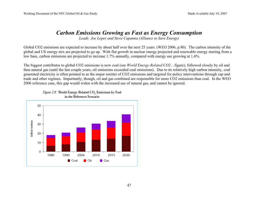
Global CO2 emissions are expected to increase by about half over the next 25 years. (WEO 2006, p.80). The carbon intensity of the global and US energy mix are projected to go up. With flat growth in nuclear energy projected and renewable energy starting from a low base, carbon emissions are projected to increase 1.7% annually, compared with energy use growing at 1.6%. The biggest contributor to global CO2 emissions is now coal (see World Energy-Related CO2…figure), followed closely by oil and then natural gas (until the last couple years, oil emissions exceeded coal emissions). Due to its relatively high carbon intensity, coal generated electricity is often pointed to as the major emitter of CO2 emissions and targeted for policy interventions through cap and trade and other regimes. Importantly, though, oil and gas combined are responsible for more CO2 emissions than coal. In the WEO 2006 reference case, this gap would widen with the increased use of natural gas, and cannot be ignored.
Working Document of the NPC Global Oil & Gas Study Made Available July 18, 2007
48
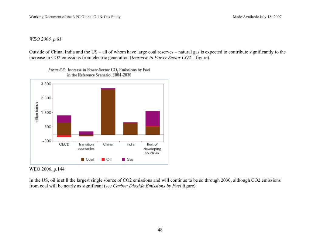
WEO 2006, p.81.
Outside of China, India and the US – all of whom have large coal reserves – natural gas is expected to contribute significantly to the increase in CO2 emissions from electric generation (Increase in Power Sector CO2…figure).
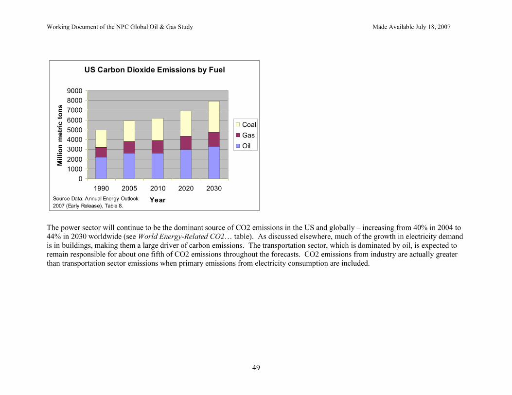
WEO 2006, p.144. In the US, oil is still the largest single source of CO2 emissions and will continue to be so through 2030, although CO2 emissions from coal will be nearly as significant (see Carbon Dioxide Emissions by Fuel figure).
Working Document of the NPC Global Oil & Gas Study Made Available July 18, 2007
49
US Carbon Dioxide Emissions by Fuel
0
1000
2000
3000
4000
5000
6000
7000
8000
9000
1990 2005 2010 2020 2030
Year
Mil
lio
n m
etr
ic t
on
s
Coal
Gas
Oil
Source Data: Annual Energy Outlook
2007 (Early Release), Table 8.
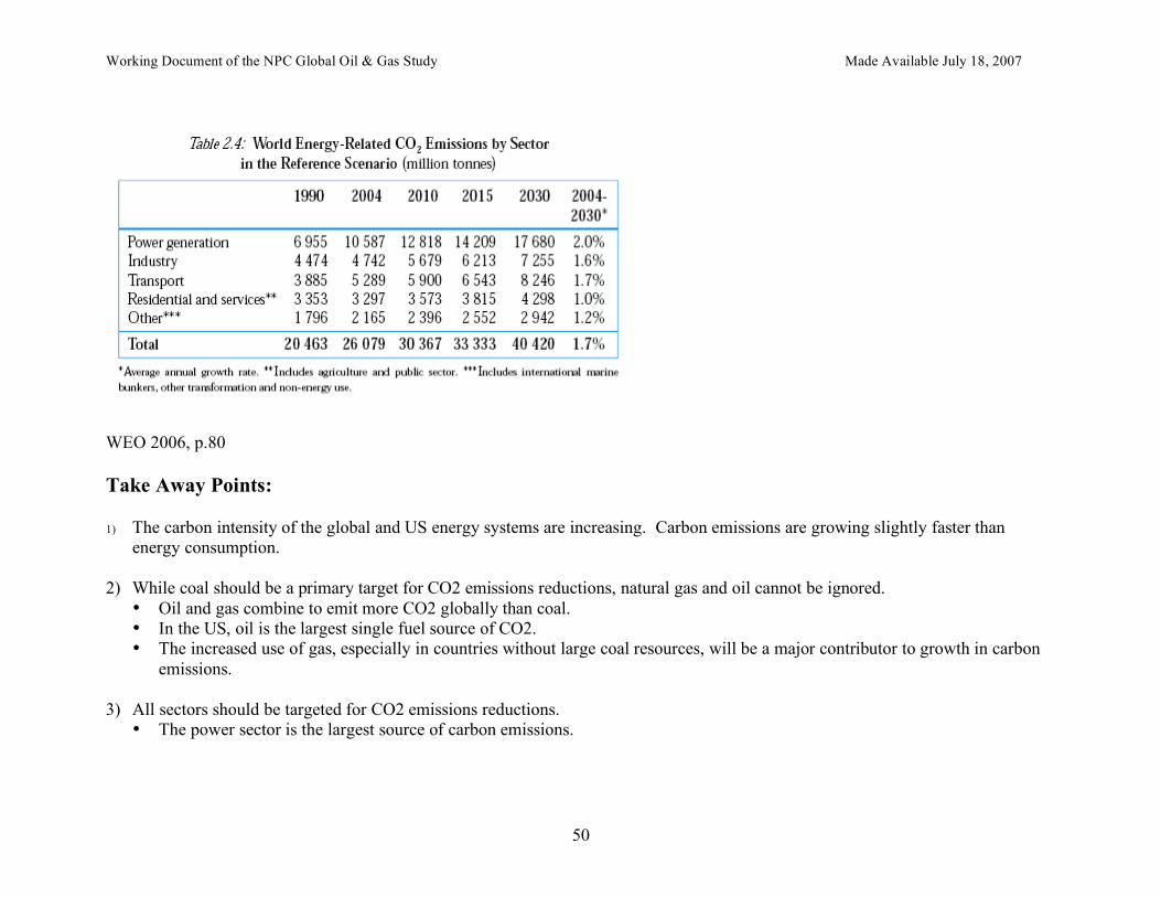
The power sector will continue to be the dominant source of CO2 emissions in the US and globally – increasing from 40% in 2004 to 44% in 2030 worldwide (see World Energy-Related CO2… table). As discussed elsewhere, much of the growth in electricity demand is in buildings, making them a large driver of carbon emissions. The transportation sector, which is dominated by oil, is expected to remain responsible for about one fifth of CO2 emissions throughout the forecasts. CO2 emissions from industry are actually greater than transportation sector emissions when primary emissions from electricity consumption are included.
Working Document of the NPC Global Oil & Gas Study Made Available July 18, 2007
50
WEO 2006, p.80
Take Away Points: 1) The carbon intensity of the global and US energy systems are increasing. Carbon emissions are growing slightly faster than
energy consumption. 2) While coal should be a primary target for CO2 emissions reductions, natural gas and oil cannot be ignored.
• Oil and gas combine to emit more CO2 globally than coal. • In the US, oil is the largest single fuel source of CO2. • The increased use of gas, especially in countries without large coal resources, will be a major contributor to growth in carbon
emissions. 3) All sectors should be targeted for CO2 emissions reductions.
• The power sector is the largest source of carbon emissions.
Working Document of the NPC Global Oil & Gas Study Made Available July 18, 2007
51
• Most of the growth in electricity demand results from the increase in electricity consumption in homes and commercial buildings.
• When emissions from electricity generation are counted, buildings are responsible for more CO2 emissions than the transportation sector.
Working Document of the NPC Global Oil & Gas Study Made Available July 18, 2007
52
China in Perspective Leads: Joe Loper and Steve Capanna (Alliance to Save Energy)
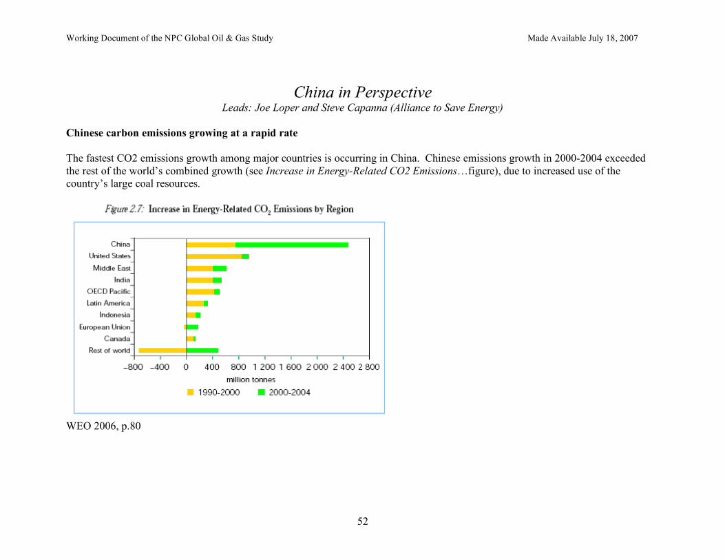
Chinese carbon emissions growing at a rapid rate The fastest CO2 emissions growth among major countries is occurring in China. Chinese emissions growth in 2000-2004 exceeded the rest of the world’s combined growth (see Increase in Energy-Related CO2 Emissions…figure), due to increased use of the country’s large coal resources.
WEO 2006, p.80
Working Document of the NPC Global Oil & Gas Study Made Available July 18, 2007
53
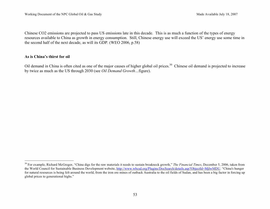
Chinese CO2 emissions are projected to pass US emissions late in this decade. This is as much a function of the types of energy resources available to China as growth in energy consumption. Still, Chinese energy use will exceed the US’ energy use some time in the second half of the next decade, as will its GDP. (WEO 2006, p.58) As is China’s thirst for oil Oil demand in China is often cited as one of the major causes of higher global oil prices.30 Chinese oil demand is projected to increase by twice as much as the US through 2030 (see Oil Demand Growth…figure).
30 For example, Richard McGregor, “China digs for the raw materials it needs to sustain breakneck growth,” The Financial Times, December 5, 2006, taken from the World Council for Sustainable Business Development website, http://www.wbcsd.org/Plugins/DocSearch/details.asp?ObjectId=MjIwMDU. “China's hunger for natural resources is being felt around the world, from the iron ore mines of outback Australia to the oil fields of Sudan, and has been a big factor in forcing up global prices to generational highs.”
Working Document of the NPC Global Oil & Gas Study Made Available July 18, 2007
54
Oil Demand Growth by 2030 (mbd)
China
USA
0
1
2
3
4
5
6
7
8
9
10
Source: IEA World Energy Outlook 2006, Table 3.1
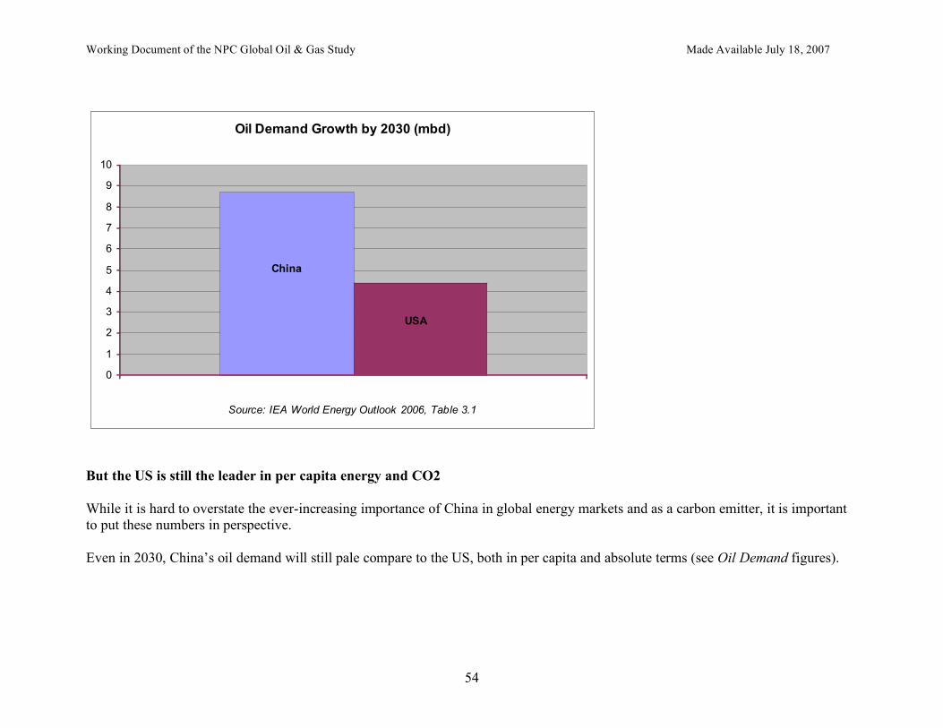
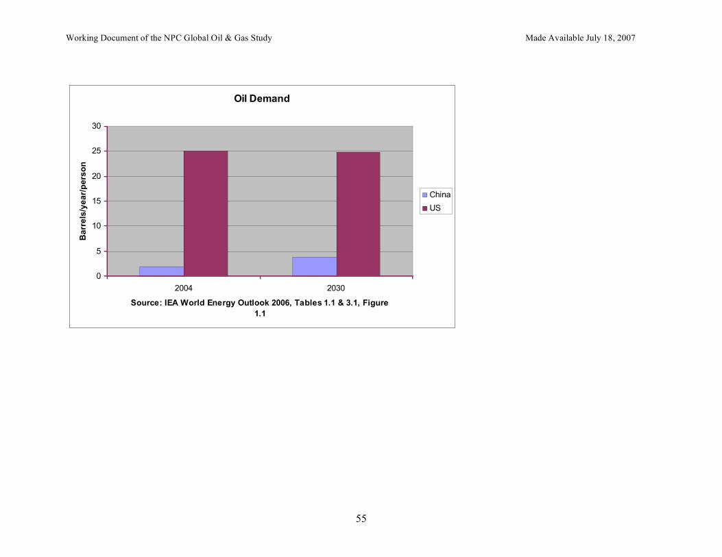
But the US is still the leader in per capita energy and CO2 While it is hard to overstate the ever-increasing importance of China in global energy markets and as a carbon emitter, it is important to put these numbers in perspective. Even in 2030, China’s oil demand will still pale compare to the US, both in per capita and absolute terms (see Oil Demand figures).
Working Document of the NPC Global Oil & Gas Study Made Available July 18, 2007
55
Oil Demand
0
5
10
15
20
25
30
2004 2030
Source: IEA World Energy Outlook 2006, Tables 1.1 & 3.1, Figure
1.1
Ba
rre
ls/y
ea
r/p
ers
on
China
US
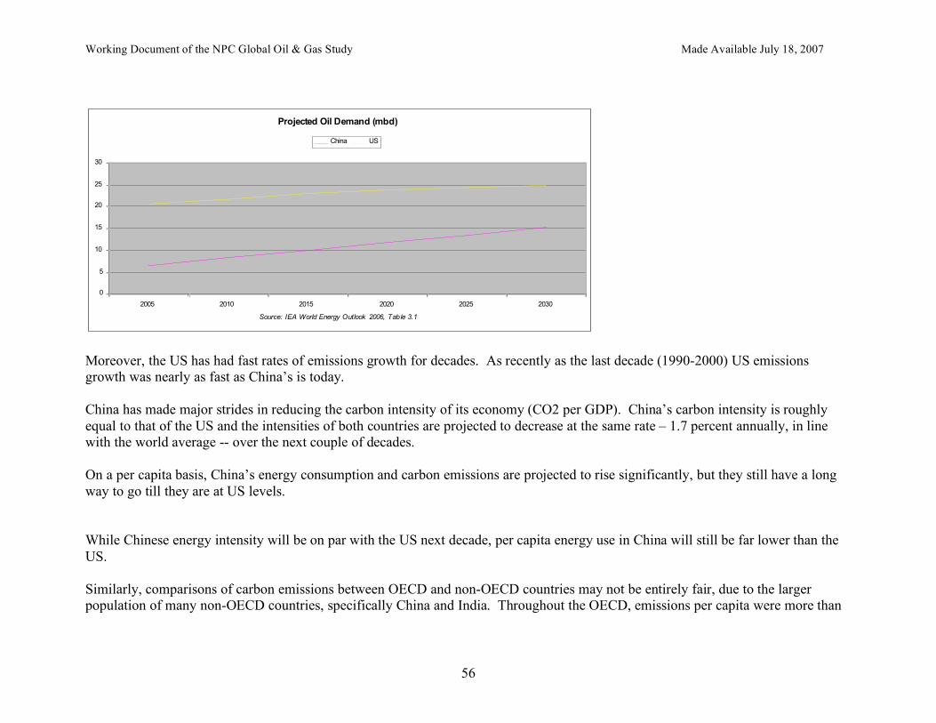
Working Document of the NPC Global Oil & Gas Study Made Available July 18, 2007
56
Projected Oil Demand (mbd)
0
5
10
15
20
25
30
2005 2010 2015 2020 2025 2030
Source: IEA World Energy Outlook 2006, Table 3.1
China US
Moreover, the US has had fast rates of emissions growth for decades. As recently as the last decade (1990-2000) US emissions growth was nearly as fast as China’s is today. China has made major strides in reducing the carbon intensity of its economy (CO2 per GDP). China’s carbon intensity is roughly equal to that of the US and the intensities of both countries are projected to decrease at the same rate – 1.7 percent annually, in line with the world average -- over the next couple of decades. On a per capita basis, China’s energy consumption and carbon emissions are projected to rise significantly, but they still have a long way to go till they are at US levels. While Chinese energy intensity will be on par with the US next decade, per capita energy use in China will still be far lower than the US. Similarly, comparisons of carbon emissions between OECD and non-OECD countries may not be entirely fair, due to the larger population of many non-OECD countries, specifically China and India. Throughout the OECD, emissions per capita were more than
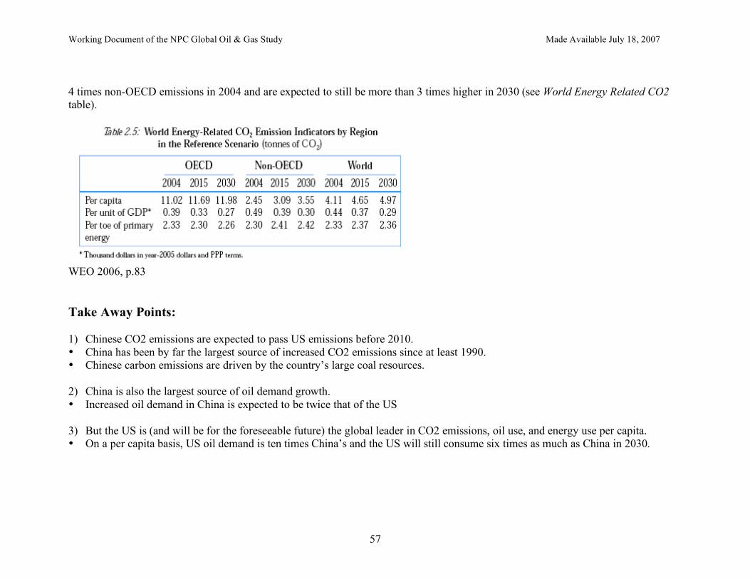
Working Document of the NPC Global Oil & Gas Study Made Available July 18, 2007
57
4 times non-OECD emissions in 2004 and are expected to still be more than 3 times higher in 2030 (see World Energy Related CO2 table).
WEO 2006, p.83 Take Away Points: 1) Chinese CO2 emissions are expected to pass US emissions before 2010. • China has been by far the largest source of increased CO2 emissions since at least 1990. • Chinese carbon emissions are driven by the country’s large coal resources. 2) China is also the largest source of oil demand growth. • Increased oil demand in China is expected to be twice that of the US 3) But the US is (and will be for the foreseeable future) the global leader in CO2 emissions, oil use, and energy use per capita. • On a per capita basis, US oil demand is ten times China’s and the US will still consume six times as much as China in 2030.
Working Document of the NPC Global Oil & Gas Study Made Available July 18, 2007
58
The Information Age – Boon or Bane? Leads: Joe Loper and Steve Capanna (Alliance to Save Energy)
Information technologies are an integral part of people’s lives throughout the world, especially in developed countries. Massive computational power and data storage, combined with global networking, has facilitated enormous improvements in living standards through, medical science breakthroughs, improved disaster preparedness, education of poor people in remote areas, on-line shopping and banking, and instant written communications and access to music and videos. There are any number of ways that information technologies could be used to reduce energy consumption, including telecommuting, dematerialization (e.g., the paperless office), and energy-efficient digital control systems in cars, buildings and factories. In addition, conventional wisdom holds that the information-based economy is less energy intensive than the economy as a whole. The rapid penetration of information technologies in the economy has led some observers to predict accelerated reductions in US and global energy intensity. The implications, if such predictions were to come to pass, are not always clear. By definition, energy use per dollar of GDP would be lower. But does it mean that energy use (or related carbon dioxide emissions and other impacts) will be lower as a result? Could absolute energy consumption actually increase (both compared to current levels and/or compared to future baseline levels) as increased plug loads are enabled by new information technologies (e.g. computers and peripherals, mp3 players, cell phones)? Could energy demand actually increase as economies boom in response to the new business and consumption opportunities created by information technologies? Could the efficiencies that information technologies deliver be less than the new energy uses that information technologies create? Of course, there is no way to put the information age genie back in the bottle, even if we wanted to. At the same time, we should be careful not to be overly optimistic that information technologies will help, rather than hinder, efforts to reduce energy demand and carbon emissions. While the notion that technology development will lead to net reductions in energy use is seductive (we could have our cake and eat it too), is it proven, or even likely? Increased electric plug loads associated with computers and other types of office equipment and growing energy demand resulting from increased economic growth fueled by new information technologies could induce a net increase in energy demand rather than a net decrease.
Working Document of the NPC Global Oil & Gas Study Made Available July 18, 2007
59
Without government intervention to encourage information technologies to be used to reduce energy consumption, they could prove to be a boon to the economy (at least in the short run) and a bane for reducing energy use (which could have adverse consequences on the economy in the long run). This article attempts to shine some light on this subject, focusing on the following questions specifically:
1. How much energy is being saved by information technologies? What evidence (anecdotal or otherwise) exists that information technologies are contributing significantly to improved energy efficiency and reduced energy intensity?
2. How much energy is being consumed directly by information technologies (e.g., computers, office equipment, data servers)? 3. How much energy is being consumed as a result of economic growth induced by information technologies?
IT Potential to Reduce Energy Use Computers and the internet have enormous potential to increase energy efficiency economy-wide through improved management and control of energy-using systems in utilities, industry, buildings and vehicles. For instance, by using advanced two-way interval meters, large commercial facilities can manage their electric loads, develop more sophisticated bill allocation practices and identify and eliminate energy leaks. The savings from these measures can easily exceed the amount of energy used to power the meters. IT has the potential to decrease the demand for energy in other ways as well. For example, roughly 30 million Americans (80 million people worldwide) telecommute at least once a month, reducing gasoline use. In Finland, more than ten percent of workers telecommute at least one day per week as do four percent of workers in Western Europe overall (See Table 3). Still, potential for increased telecommuting is significant, though not huge. In the US, more than 97 million workers (76%) drive to work alone, and only 3.2% work at home. If half of car commuters telecommuted one day per week – or used flex time scheduling – commuting VMT (vehicle miles traveled) could potentially be reduced by 20% and total personal vehicle VMT could be reduced by about 5% nationally (commuting is about 27% of personal VMT), saving almost a quad annually.31
31 DOE, Transportation Energy Data Book, 25th Edition, Oak Ridge National Laboratory, 2006, Tables 2.1 and 8.8.
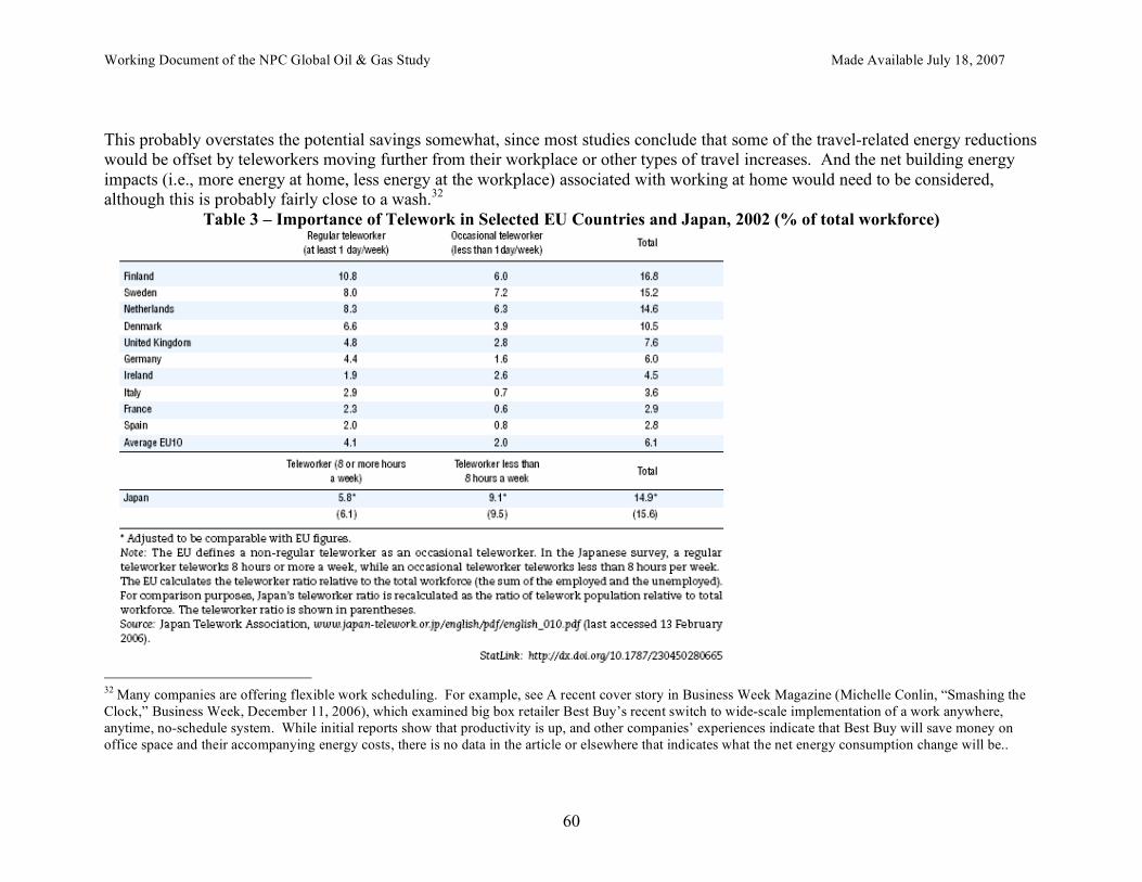
Working Document of the NPC Global Oil & Gas Study Made Available July 18, 2007
60
This probably overstates the potential savings somewhat, since most studies conclude that some of the travel-related energy reductions would be offset by teleworkers moving further from their workplace or other types of travel increases. And the net building energy impacts (i.e., more energy at home, less energy at the workplace) associated with working at home would need to be considered, although this is probably fairly close to a wash.32
Table 3 – Importance of Telework in Selected EU Countries and Japan, 2002 (% of total workforce)
32 Many companies are offering flexible work scheduling. For example, see A recent cover story in Business Week Magazine (Michelle Conlin, “Smashing the Clock,” Business Week, December 11, 2006), which examined big box retailer Best Buy’s recent switch to wide-scale implementation of a work anywhere, anytime, no-schedule system. While initial reports show that productivity is up, and other companies’ experiences indicate that Best Buy will save money on office space and their accompanying energy costs, there is no data in the article or elsewhere that indicates what the net energy consumption change will be..
Working Document of the NPC Global Oil & Gas Study Made Available July 18, 2007
61
There could also be reduced travel associated with online shopping. In some sectors, internet sales are already a significant part of business. Overall, internet sales represented about $170 billion in 2005 alone (22 percent more than in 2004)33 and $30 billion just during the holiday season.34 Sector sales from the internet in 2005 were, for: computer hardware and software (48%), tickets (28%), travel (26%), books (20%), consumer electronics (13%), cosmetics and fragrances (12%), toys and video games (12%), and flowers, cards, and gifts (10%).35 Some music, too, is increasingly being purchased via the internet, as evidenced by the success of iTunes and the demise of traditional retailers (e.g., Tower Records). Unfortunately, we have seen no studies of the impacts of online sales on energy consumption and dematerialization. It’s actually not clear whether the impacts are even positive – whether a UPS truck consumes more fuel per package than a shopper (who may buy numerous items on a trip) is unclear. Likewise, to our knowledge there are no studies examining other forms of dematerialization, including the savings from reduction of newspaper printing as more people get their news online, online bill paying, etc. And according to the Direct Marketing Association, companies mailed 19.16 billion catalogs in 2006, up 15% from 2000 – customers apparently like to browse catalogs before buying online.36 IT-related Energy Consumption Plug loads associated with computers, office equipment, and the internet have increased over the last several years, and will continue to increase for at least the next fifteen years in the US,37 and for much longer than that globally. EIA estimates that primary electricity consumption of residential and commercial personal computers in the US was about 80 TWh in 2005 and that it will increase to around 170 TWh by 2020, when consumption growth in the commercial sector will flatten while the
33 Shop.org, “Online Retail Sales, Profitablity Continue Climb, According to Shop.org/Forrester Research,” May 24, 2005, http://www.shop.org/press/05/052405.asp. 34 Internet shopping represented either 6 or 7 percent of holiday shopping sales. Either 23% more than 2005 to $27 billion or 18% more than 2005 to $32 billion, depending on which research group you trust. http://www.signonsandiego.com/news/business/20061126-9999-mz1b26shoppi.html . Or https://mr.pricegrabber.com/december_2006_holiday_shopping_trends.pdf. 35 Shop.org. 36 Amy Merrick, “Victoria’s Secret Goes Green on Paper for Catalogs,” Wall Street Journal, December 7, 2006, p. B2. 37 Energy Information Administration, Annual Energy Outlook 2007, Tables A4 & A5, http://www.eia.doe.gov/oiaf/aeo/aeoref_tab.html.
Working Document of the NPC Global Oil & Gas Study Made Available July 18, 2007
62
residential sector continues to trend upward.38 Since total US electricity consumption was equal to 3,653 TWh in 2005, PC electric consumption represents about 2 percent of current total US electric consumption.39 By 2020, total US electricity consumption is projected to be 4,844 TWh, of which PCs will account for 3.5 percent.40 According to a study prepared by TIAX LCC for the U.S. Department of Energy in March 2006, residential sector IT electricity consumption is 42 TWh annually (this includes PCs, routers, laptops, monitors, broadband access, printers and other peripherals.) Its estimate of 2005 residential PC electric consumption is 22.5 TWh, roughly equal to the AEO’s estimate for residential personal computers. Only time will tell whether current projections about information technology hold up – past reports have tended to underestimate IT energy use fairly dramatically, at least in the residential sector. The TIAX study, for example, estimates IT consumption to be more than twice an earlier estimate by LBL (Nordman and Meier, 2004),41 and about 75 percent higher than Rand (2001) projections, which projected 2006 residential IT use would be about 24 TWh. EIA’s 2001 Residential Energy Consumption Survey reported that residential PCs and printers alone were consuming roughly 23 TWh, so the RAND estimate is almost certainly low. And EIA’s 2000 Annual Energy Outlook projected that residential PC energy consumption would equal only 32 TWh in 2020, while the 2007 version is projecting 52 TWh for that same year. Our goal is not to highlight errors in previous projections, but to demonstrate that actual IT energy use tends to exceed estimates and projections. TIAX projects three different scenarios for 2010, with residential IT electricity consumption ranging from 31 TWh to 101 TWh annually. Residential desktop and laptop PC electricity consumption ranges from 14.6 TWh to 70.6 TWh depending on the projection. The wide range of TIAX’s projections highlights the importance of different policies in determining energy consumption, as well as the unpredictable nature of consumer preferences.42 According to TIAX’s “PC Reigns” scenario, which projects the highest residential IT electricity consumption, in 2010, residential IT appliances will consume 101 TWh, while residential PCs alone will consume almost 71 TWh – almost twice the 2007 AEO’s 38 EIA Annual Energy Outlook 2007, Tables A4 and A5. 39 EIA Annual Energy Review 2005, Table 8.9. 40 EIA Annual Energy Outlook 2005, Table 8. 41 As quoted in the TIAX study 42 Two of the three projections (the “Ubiquitous” and “Greening” scenarios) predict fewer residential desktop PCs in 2010 than in 2005, although all three scenarios predict an increase in the number of laptop computers.
Working Document of the NPC Global Oil & Gas Study Made Available July 18, 2007
63
projected residential PC electricity consumption for 2010. The range of these relatively recent TIAX projections is far higher than previous projections, for example by Rand (2001), which projected residential computer equipment to consume roughly 25 TWh in 2021 in its reference case.43 The 2007 AEO estimates current electricity use by information and communications equipment in the commercial sector to be around 170 TWh per year. Using the TIAX residential estimates, residential and commercial information technology equipment currently use about 210 TWh, or about 5 percent of US electricity consumption. IT a Relatively Small, but Rapidly Growing, Share of Energy Use While IT energy use is growing rapidly, it still appears to be a relatively small portion of overall electricity use (five percent of US and two percent of global energy consumption). Through 2030, EIA projects residential energy use from PCs to increase nearly 4 percent annually, far faster than any other end-use category. PC energy use is expected to more than double by 2030 compared to less than a 40% increase in overall electric use. Still, energy consumption from PCs will increase by less than 40 TWh between 2005 and 2030, which is less than the predicted increase in energy use for lighting, televisions, heating, or “other” (undefined) end-uses (Figure 6). Computers and office equipment, along with other IT-related energy use lumped into the “other” category (e.g., telecommunications equipment), could comprise the majority of increased electricity consumption in commercial buildings from 2005-2030 (Figure 7).
43 Although RAND has four 2021 scenarios, in each of them residential computer equipment electricity consumption is lower than what was predicted for 2021 by the 2001 AEO.
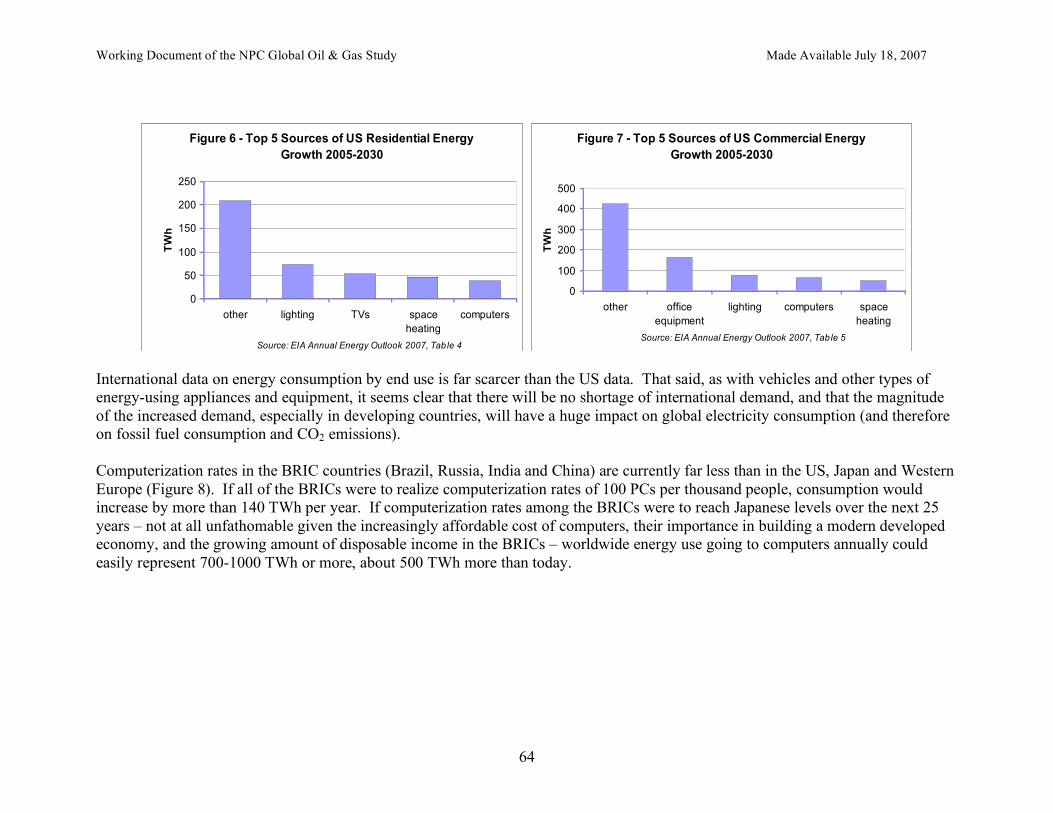
Working Document of the NPC Global Oil & Gas Study Made Available July 18, 2007
64
Figure 6 - Top 5 Sources of US Residential Energy
Growth 2005-2030
0
50
100
150
200
250
other lighting TVs space
heating
computers
Source: EIA Annual Energy Outlook 2007, Table 4
TW
h
Figure 7 - Top 5 Sources of US Commercial Energy
Growth 2005-2030
0
100
200
300
400
500
other office
equipment
lighting computers space
heating
Source: EIA Annual Energy Outlook 2007, Table 5
TW
h
International data on energy consumption by end use is far scarcer than the US data. That said, as with vehicles and other types of energy-using appliances and equipment, it seems clear that there will be no shortage of international demand, and that the magnitude of the increased demand, especially in developing countries, will have a huge impact on global electricity consumption (and therefore on fossil fuel consumption and CO2 emissions). Computerization rates in the BRIC countries (Brazil, Russia, India and China) are currently far less than in the US, Japan and Western Europe (Figure 8). If all of the BRICs were to realize computerization rates of 100 PCs per thousand people, consumption would increase by more than 140 TWh per year. If computerization rates among the BRICs were to reach Japanese levels over the next 25 years – not at all unfathomable given the increasingly affordable cost of computers, their importance in building a modern developed economy, and the growing amount of disposable income in the BRICs – worldwide energy use going to computers annually could easily represent 700-1000 TWh or more, about 500 TWh more than today.
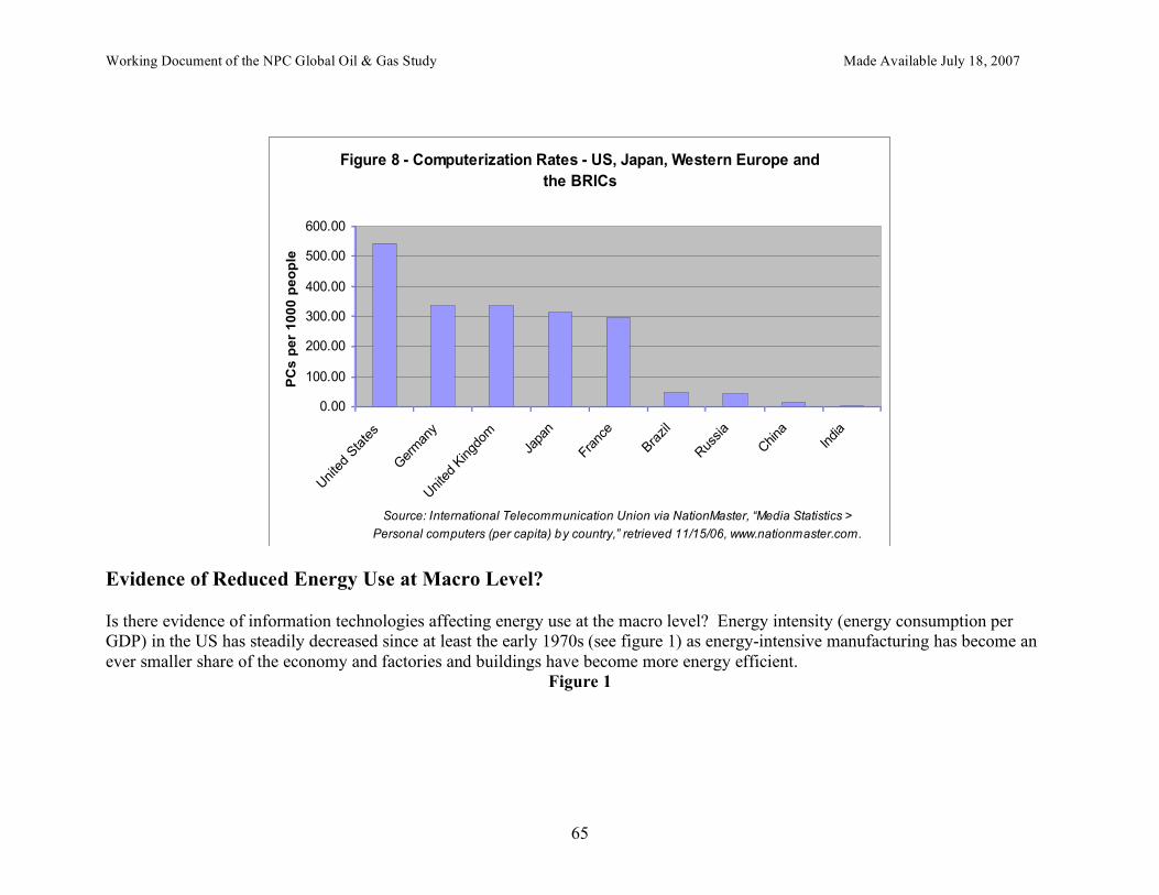
Working Document of the NPC Global Oil & Gas Study Made Available July 18, 2007
65
Figure 8 - Computerization Rates - US, Japan, Western Europe and
the BRICs
0.00
100.00
200.00
300.00
400.00
500.00
600.00
Unite
d Sta
tes
Ger
man
y
Unite
d Kingd
om
Japa
n
Franc
e
Bra
zil
Rus
sia
China
India
Source: International Telecommunication Union via NationMaster, “Media Statistics >
Personal computers (per capita) by country,” retrieved 11/15/06, www.nationmaster.com.
PC
s p
er
10
00
pe
op
le
Evidence of Reduced Energy Use at Macro Level? Is there evidence of information technologies affecting energy use at the macro level? Energy intensity (energy consumption per GDP) in the US has steadily decreased since at least the early 1970s (see figure 1) as energy-intensive manufacturing has become an ever smaller share of the economy and factories and buildings have become more energy efficient.
Figure 1
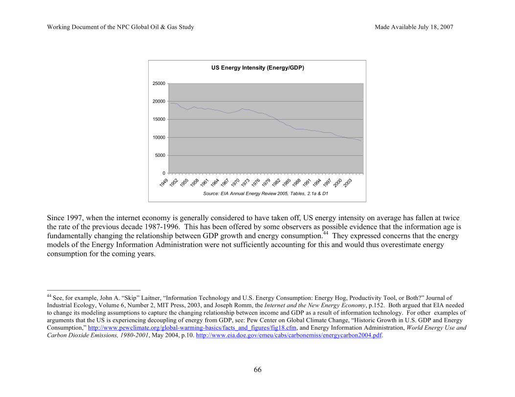
Working Document of the NPC Global Oil & Gas Study Made Available July 18, 2007
66
US Energy Intensity (Energy/GDP)
0
5000
10000
15000
20000
25000
1949
1952
1955
1958
1961
1964
1967
1970
1973
1976
1979
1982
1985
1988
1991
1994
1997
2000
2003
Source: EIA Annual Energy Review 2005, Tables, 2.1a & D1
Since 1997, when the internet economy is generally considered to have taken off, US energy intensity on average has fallen at twice the rate of the previous decade 1987-1996. This has been offered by some observers as possible evidence that the information age is fundamentally changing the relationship between GDP growth and energy consumption.44 They expressed concerns that the energy models of the Energy Information Administration were not sufficiently accounting for this and would thus overestimate energy consumption for the coming years.
44 See, for example, John A. “Skip” Laitner, “Information Technology and U.S. Energy Consumption: Energy Hog, Productivity Tool, or Both?” Journal of Industrial Ecology, Volume 6, Number 2, MIT Press, 2003, and Joseph Romm, the Internet and the New Energy Economy, p.152. Both argued that EIA needed to change its modeling assumptions to capture the changing relationship between income and GDP as a result of information technology. For other examples of arguments that the US is experiencing decoupling of energy from GDP, see: Pew Center on Global Climate Change, “Historic Growth in U.S. GDP and Energy Consumption,” http://www.pewclimate.org/global-warming-basics/facts_and_figures/fig18.cfm, and Energy Information Administration, World Energy Use and Carbon Dioxide Emissions, 1980-2001, May 2004, p.10. http://www.eia.doe.gov/emeu/cabs/carbonemiss/energycarbon2004.pdf.
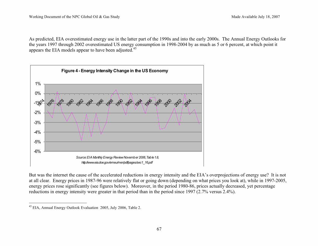
Working Document of the NPC Global Oil & Gas Study Made Available July 18, 2007
67
As predicted, EIA overestimated energy use in the latter part of the 1990s and into the early 2000s. The Annual Energy Outlooks for the years 1997 through 2002 overestimated US energy consumption in 1998-2004 by as much as 5 or 6 percent, at which point it appears the EIA models appear to have been adjusted.45
Figure 4 - Energy Intensity Change in the US Economy
-6%
-5%
-4%
-3%
-2%
-1%
0%
1%
1974
1976
1978
1980
1982
1984
1986
1988
1990
1992
1994
1996
1998
2000
2002
2004
Source: EIA Monthly Energy Review November 2006, Table 1.8,
http://www.eia.doe.gov/emeu/mer/pdf/pages/sec1_16.pdf But was the internet the cause of the accelerated reductions in energy intensity and the EIA’s overprojections of energy use? It is not at all clear. Energy prices in 1987-96 were relatively flat or going down (depending on what prices you look at), while in 1997-2005, energy prices rose significantly (see figures below). Moreover, in the period 1980-86, prices actually decreased, yet percentage reductions in energy intensity were greater in that period than in the period since 1997 (2.7% versus 2.4%).
45 EIA, Annual Energy Outlook Evaluation 2005, July 2006, Table 2.
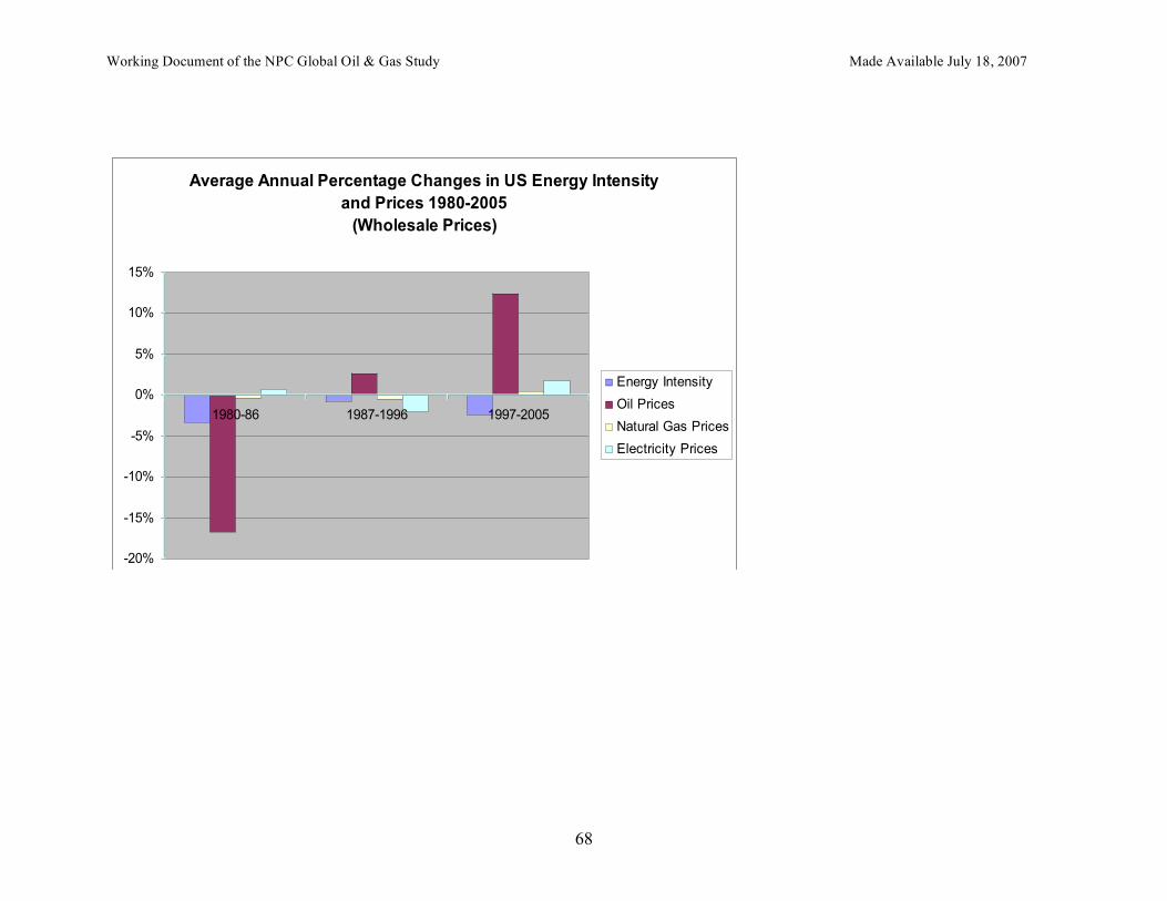
Working Document of the NPC Global Oil & Gas Study Made Available July 18, 2007
68
Average Annual Percentage Changes in US Energy Intensity
and Prices 1980-2005
(Wholesale Prices)
-20%
-15%
-10%
-5%
0%
5%
10%
15%
1980-86 1987-1996 1997-2005
Energy Intensity
Oil Prices
Natural Gas Prices
Electricity Prices
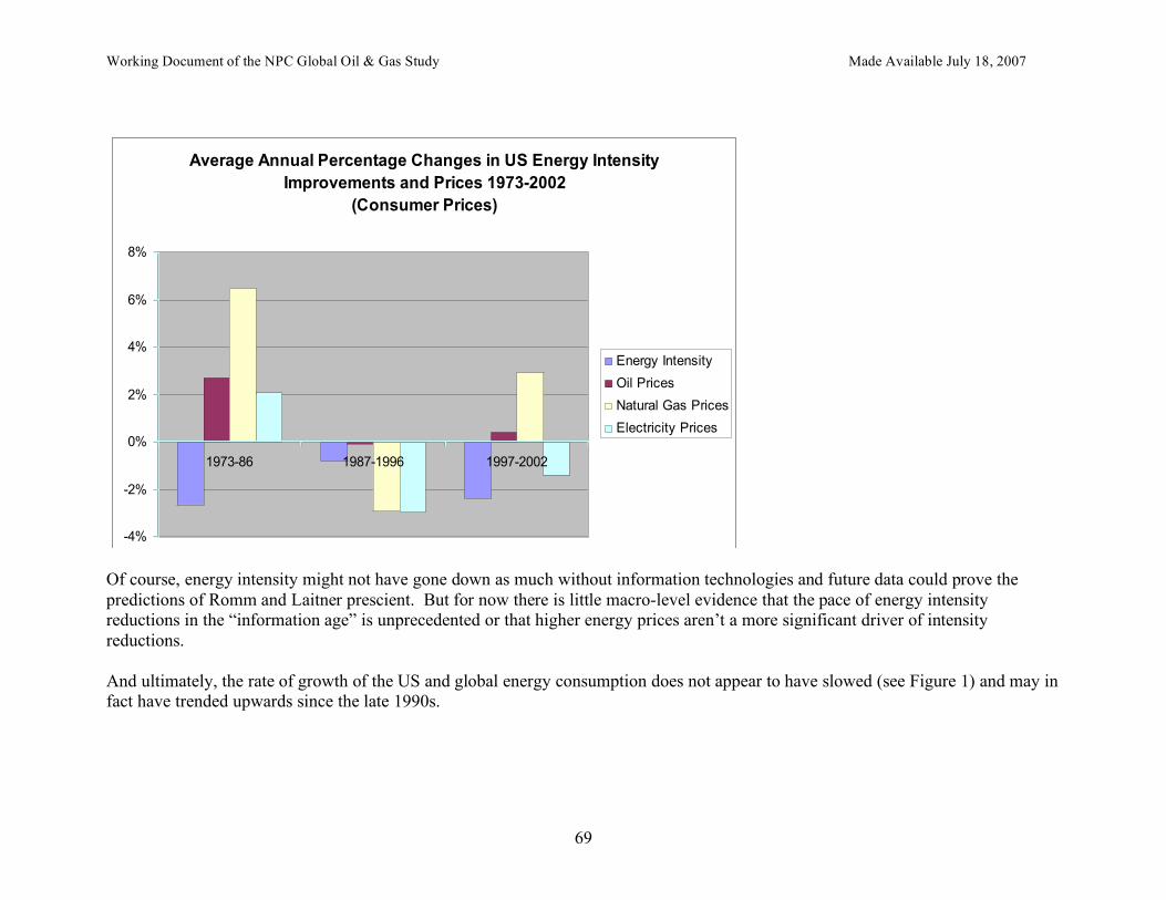
Working Document of the NPC Global Oil & Gas Study Made Available July 18, 2007
69
Average Annual Percentage Changes in US Energy Intensity
Improvements and Prices 1973-2002
(Consumer Prices)
-4%
-2%
0%
2%
4%
6%
8%
1973-86 1987-1996 1997-2002
Energy Intensity
Oil Prices
Natural Gas Prices
Electricity Prices
Of course, energy intensity might not have gone down as much without information technologies and future data could prove the predictions of Romm and Laitner prescient. But for now there is little macro-level evidence that the pace of energy intensity reductions in the “information age” is unprecedented or that higher energy prices aren’t a more significant driver of intensity reductions. And ultimately, the rate of growth of the US and global energy consumption does not appear to have slowed (see Figure 1) and may in fact have trended upwards since the late 1990s.
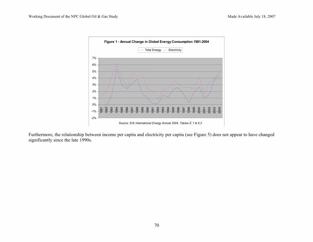
Working Document of the NPC Global Oil & Gas Study Made Available July 18, 2007
70
Figure 1 - Annual Change in Global Energy Consumption 1981-2004
-2%
-1%
0%
1%
2%
3%
4%
5%
6%
7%
1981
1982
1983
1984
1985
1986
1987
1988
1989
1990
1991
1992
1993
1994
1995
1996
1997
1998
1999
2000
2001
2002
2003
2004
Source: EIA International Energy Annual 2004, Tables E.1 & 6.2
Total Energy Electricity
Furthermore, the relationship between income per capita and electricity per capita (see Figure 5) does not appear to have changed significantly since the late 1990s.
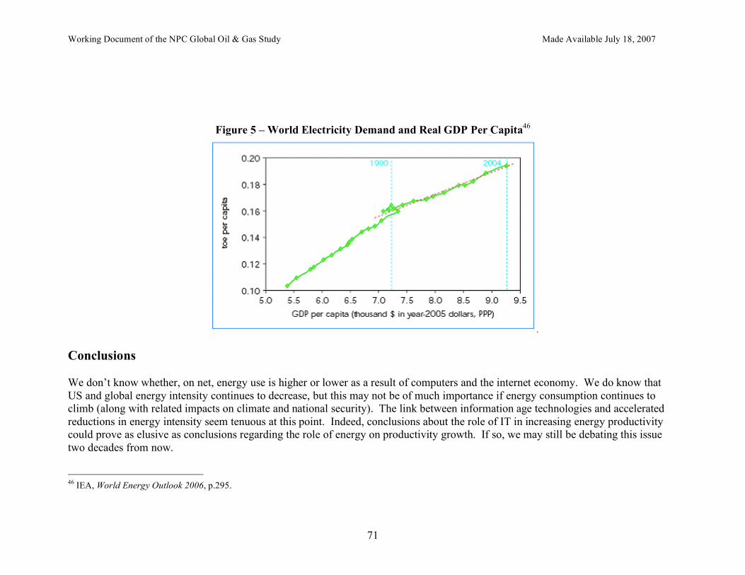
Working Document of the NPC Global Oil & Gas Study Made Available July 18, 2007
71
Figure 5 – World Electricity Demand and Real GDP Per Capita46
. Conclusions We don’t know whether, on net, energy use is higher or lower as a result of computers and the internet economy. We do know that US and global energy intensity continues to decrease, but this may not be of much importance if energy consumption continues to climb (along with related impacts on climate and national security). The link between information age technologies and accelerated reductions in energy intensity seem tenuous at this point. Indeed, conclusions about the role of IT in increasing energy productivity could prove as elusive as conclusions regarding the role of energy on productivity growth. If so, we may still be debating this issue two decades from now. 46 IEA, World Energy Outlook 2006, p.295.

Working Document of the NPC Global Oil & Gas Study Made Available July 18, 2007
72
But the importance of this issue is not diminished by its difficulty. On the one hand, overestimating future energy demand (by not accounting for information technologies’ potential to make the global economy more energy efficient) could lead to overdevelopment of energy supplies, in which case suppliers could be induced to encourage greater energy demand to rid themselves of excess capacity. On the other hand, if excessive optimism causes us to underestimate future energy demand requirements, we could be forced to develop new energy sources hastily in the future, at potentially great financial and environmental costs. And overly optimistic predictions that information technology (or any other technology) will reduce our reliance on fossil fuels might send the message that addressing energy challenges will not require any hard choices. There are seemingly few historical precedents for new technologies actually reducing energy use (as opposed to just reducing energy intensity). New technologies often create new service demands at the same time they improve the efficiency of existing service demands – the technology has the potential to reduce energy use, but gets called on for other purposes or allows (even encourages) increased demand for new and additional energy services.47 The point is that we cannot count on technology – information age or other – to autonomously reduce energy use (and related impacts on the climate and national security). Without significant government policies, including (depending on the objective) significant taxes and regulations, to force technologies to be used for reducing energy, there seems every likelihood that the technologies will be used in ways that increase energy use instead.
47 Many examples come to mind: vehicle fuel efficiency has increased, but vehicle fuel economies stay the same as vehicles become heavier and more powerful and have more amenities; as refrigerator efficiencies have increased, so have their size, the number of amenities and households with two refrigerators; homes have become more efficient but bigger.
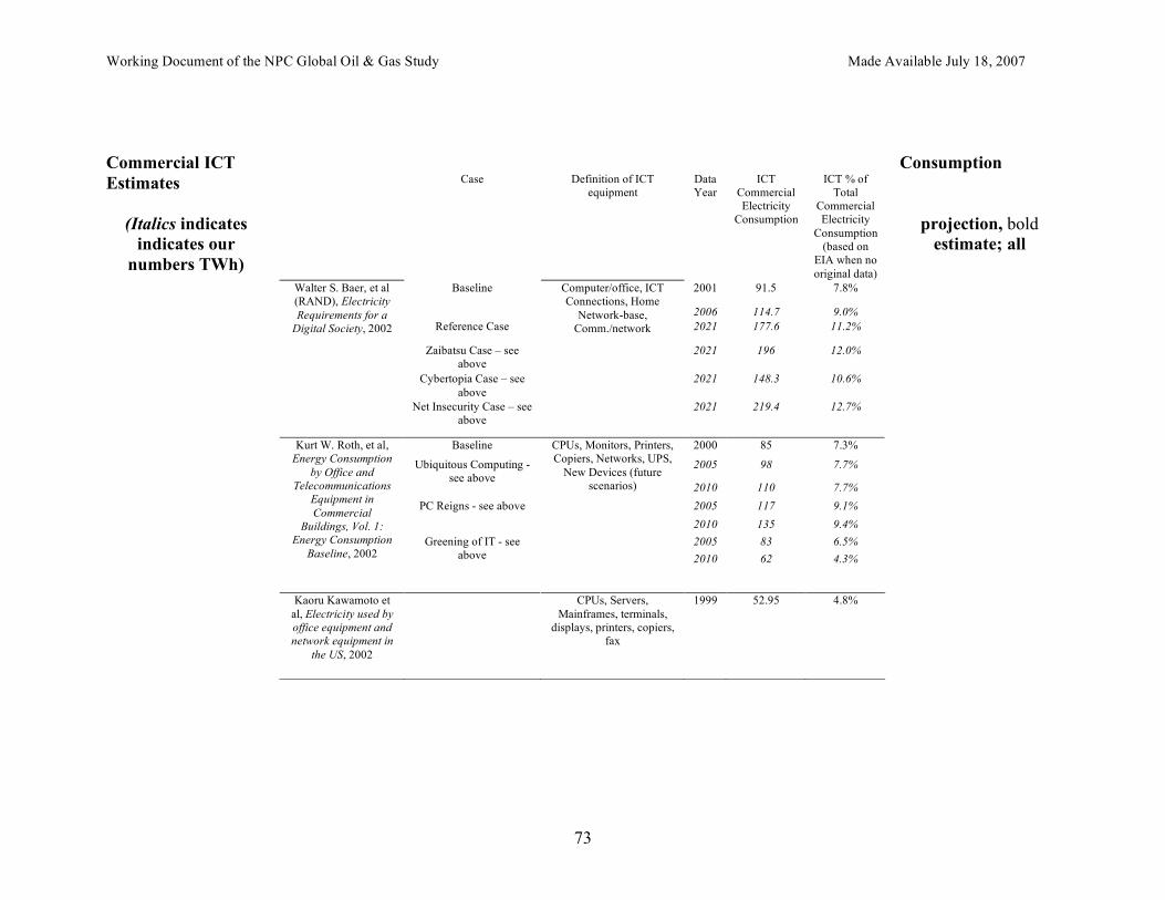
Working Document of the NPC Global Oil & Gas Study Made Available July 18, 2007
73
Commercial ICT Consumption Estimates
(Italics indicates projection, bold
indicates our estimate; all numbers TWh)
Case Definition of ICT equipment
Data Year
ICT Commercial Electricity
Consumption
ICT % of Total
Commercial Electricity
Consumption (based on
EIA when no original data)
2001 91.5 7.8% Baseline
2006 114.7 9.0% Reference Case 2021 177.6 11.2%
Zaibatsu Case – see above
2021 196 12.0%
Cybertopia Case – see above
2021 148.3 10.6%
Walter S. Baer, et al (RAND), Electricity Requirements for a
Digital Society, 2002
Net Insecurity Case – see above
Computer/office, ICT Connections, Home
Network-base, Comm./network
2021 219.4 12.7%
Baseline 2000 85 7.3%
2005 98 7.7% Ubiquitous Computing - see above
2010 110 7.7% 2005 117 9.1% PC Reigns - see above 2010 135 9.4% 2005 83 6.5%
Kurt W. Roth, et al, Energy Consumption
by Office and Telecommunications
Equipment in Commercial
Buildings, Vol. 1: Energy Consumption
Baseline, 2002 Greening of IT - see
above
CPUs, Monitors, Printers, Copiers, Networks, UPS,
New Devices (future scenarios)
2010 62 4.3%
Kaoru Kawamoto et al, Electricity used by office equipment and network equipment in
the US, 2002
CPUs, Servers, Mainframes, terminals,
displays, printers, copiers, fax
1999 52.95 4.8%
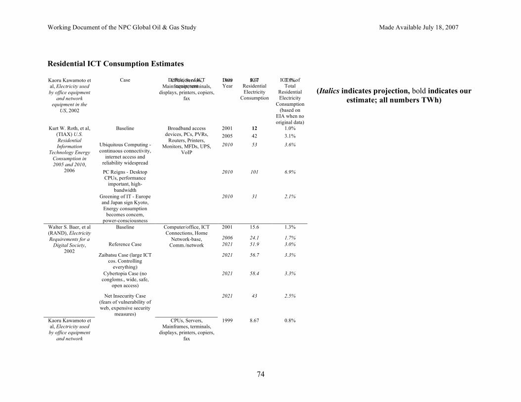
Working Document of the NPC Global Oil & Gas Study Made Available July 18, 2007
74
Residential ICT Consumption Estimates
(Italics indicates projection, bold indicates our
estimate; all numbers TWh)
Case Definition of ICT equipment
Data Year
ICT Residential Electricity
Consumption
ICT % of Total
Residential Electricity
Consumption (based on
EIA when no original data)
2001 12 1.0% Baseline 2005 42 3.1%
Ubiquitous Computing - continuous connectivity,
internet access and reliability widespread
2010 53 3.6%
PC Reigns - Desktop CPUs, performance
important, high-bandwidth
2010 101 6.9%
Kurt W. Roth, et al, (TIAX) U.S. Residential Information
Technology Energy Consumption in 2005 and 2010,
2006
Greening of IT - Europe and Japan sign Kyoto, Energy consumption
becomes concern, power-consciousness
Broadband access devices, PCs, PVRs,
Routers, Printers, Monitors, MFDs, UPS,
VoIP
2010 31 2.1%
2001 15.6 1.3% Baseline
2006 24.1 1.7% Reference Case 2021 51.9 3.0%
Zaibatsu Case (large ICT cos. Controlling
everything)
2021 56.7 3.3%
Cybertopia Case (no congloms., wide, safe,
open access)
2021 58.4 3.3%
Walter S. Baer, et al (RAND), Electricity Requirements for a
Digital Society, 2002
Net Insecurity Case (fears of vulnerability of web, expensive security
measures)
Computer/office, ICT Connections, Home
Network-base, Comm./network
2021 43 2.5%
Kaoru Kawamoto et al, Electricity used by office equipment
and network equipment in the
US, 2002
CPUs, Servers, Mainframes, terminals,
displays, printers, copiers, fax
1999 8.67 0.8%
Kaoru Kawamoto et al, Electricity used by office equipment
and network equipment in the
US, 2002
CPUs, Servers, Mainframes, terminals,
displays, printers, copiers, fax
1999 8.67 0.8%
Working Document of the NPC Global Oil & Gas Study Made Available July 18, 2007
75
Energy Elasticities: Measuring Market Responsiveness to Income and Prices Lead: John “Skip” Laitner (American Council for an Energy Efficient Economy)
Introduction Growing demand for energy worldwide together with tight oil and gas markets has resulted in highly volatile and rapidly rising energy prices. Both rising prices and growing concerns about international energy security and global climate change have again put energy in the news. Both policymakers and business leaders want to know how much and when demand will respond to these high prices; and whether new policies and measures might stimulate the development of new energy resources and the more efficient use of existing energy resources. Conventional wisdom, for example, suggests that there will be little quantity response to these energy prices, at least in the short run. However, decades of econometric work suggests over time consumers and businesses do adjust. This paper reviews and analyzes the existing research that evaluates the responsiveness of consumers and businesses to changes in incomes, prices and policies as they all impact energy production and consumption. This document discusses historical trends in fuel switching capability and long-term fuel choice. The majority of the content focuses on the United States given the dearth of data about the rest of the world. Data on European and Asian countries are included in the discussion to the greatest extent possible. Understanding Elasticities In brief, elasticities are a measure of how a change in one variable responds to a change in another variable. Hence, elasticities are a measure of responsiveness. More formally, elasticities measure the percentage change in one variable with respect to a percentage change in another variable. Measures of elasticity tend to be carried out for relatively small changes in the variable that causes the response. For purposes of discussion, we consider four categories of demand elasticities: price, income and cross elasticities. 1. Own Price Elasticity of Demand — Price elasticity measures the change in demand for a given quantity (such as energy) that might result from a change in its own price. To avoid the measure of elasticity being sensitive to the units measured, the elasticity of demand is expressed as the percentage change in demand that occurs in response to a percentage change in its own price.
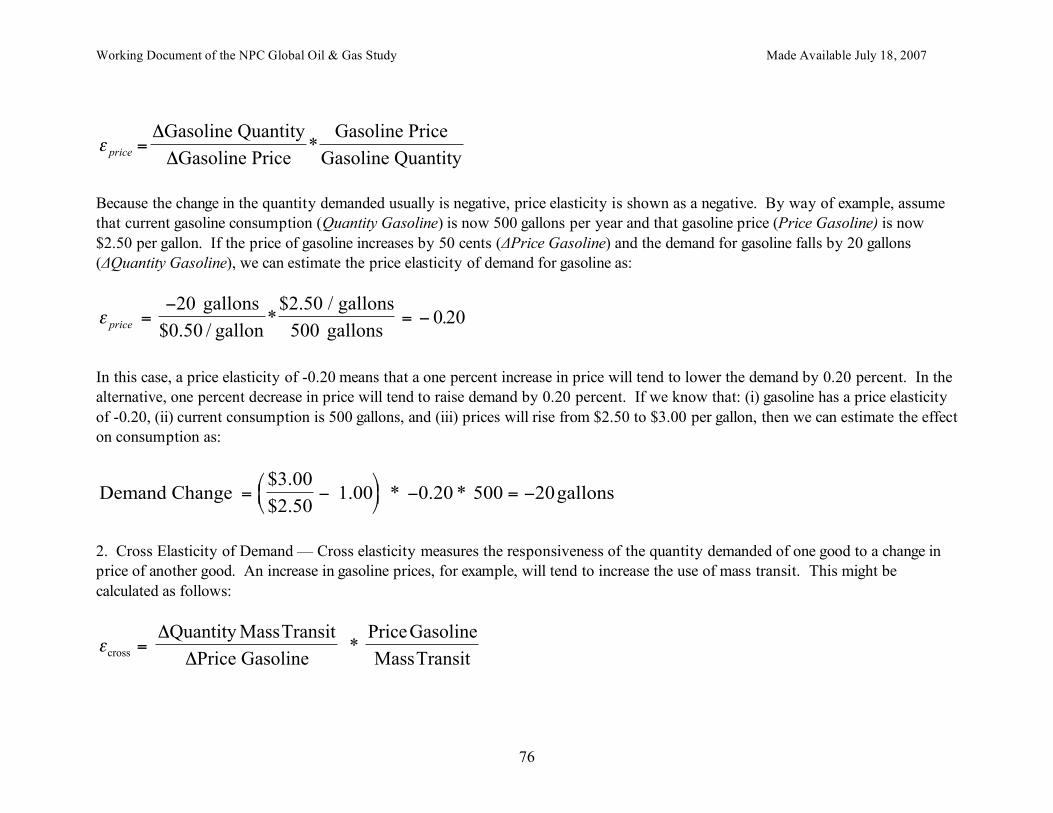
Working Document of the NPC Global Oil & Gas Study Made Available July 18, 2007
76
!price
="
"
Gasoline Quantity
Gasoline Price
Gasoline Price
Gasoline Quantity*
Because the change in the quantity demanded usually is negative, price elasticity is shown as a negative. By way of example, assume that current gasoline consumption (Quantity Gasoline) is now 500 gallons per year and that gasoline price (Price Gasoline) is now $2.50 per gallon. If the price of gasoline increases by 50 cents (ΔPrice Gasoline) and the demand for gasoline falls by 20 gallons (ΔQuantity Gasoline), we can estimate the price elasticity of demand for gasoline as:
!price
="
= "20 gallons
$0.50 / gallon
$2.50 / gallons
500 gallons* .0 20
In this case, a price elasticity of -0.20 means that a one percent increase in price will tend to lower the demand by 0.20 percent. In the alternative, one percent decrease in price will tend to raise demand by 0.20 percent. If we know that: (i) gasoline has a price elasticity of -0.20, (ii) current consumption is 500 gallons, and (iii) prices will rise from $2.50 to $3.00 per gallon, then we can estimate the effect on consumption as:
Demand Change $3.00
$2.50 1.00 * 0.20 * 500 20gallons= !
"#$
%&' ! = !
2. Cross Elasticity of Demand — Cross elasticity measures the responsiveness of the quantity demanded of one good to a change in price of another good. An increase in gasoline prices, for example, will tend to increase the use of mass transit. This might be calculated as follows:
!cross Quantity MassTransit
Price Gasoline *
PriceGasoline
MassTransit="
"
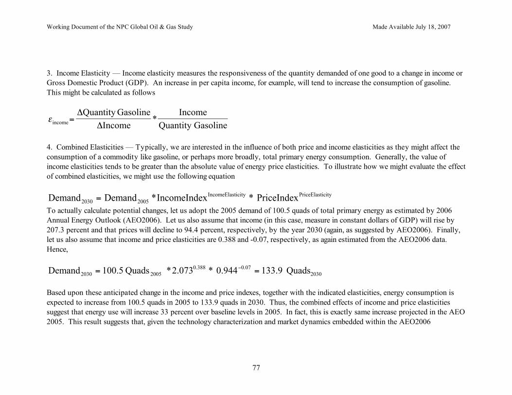
Working Document of the NPC Global Oil & Gas Study Made Available July 18, 2007
77
3. Income Elasticity — Income elasticity measures the responsiveness of the quantity demanded of one good to a change in income or Gross Domestic Product (GDP). An increase in per capita income, for example, will tend to increase the consumption of gasoline. This might be calculated as follows
!income Quantity Gasoline
Income *
Income
Quantity Gasoline="
"
4. Combined Elasticities — Typically, we are interested in the influence of both price and income elasticities as they might affect the consumption of a commodity like gasoline, or perhaps more broadly, total primary energy consumption. Generally, the value of income elasticities tends to be greater than the absolute value of energy price elasticities. To illustrate how we might evaluate the effect of combined elasticities, we might use the following equation Demand Demand *IncomeIndex * PriceIndex2030 2005
IncomeElasticity PriceElasticity=
To actually calculate potential changes, let us adopt the 2005 demand of 100.5 quads of total primary energy as estimated by 2006 Annual Energy Outlook (AEO2006). Let us also assume that income (in this case, measure in constant dollars of GDP) will rise by 207.3 percent and that prices will decline to 94.4 percent, respectively, by the year 2030 (again, as suggested by AEO2006). Finally, let us also assume that income and price elasticities are 0.388 and -0.07, respectively, as again estimated from the AEO2006 data. Hence, Demand 100.5 Quads *2.073 * 0.944 133.9 Quads2030 2005
0.388 0.07
2030= =!
Based upon these anticipated change in the income and price indexes, together with the indicated elasticities, energy consumption is expected to increase from 100.5 quads in 2005 to 133.9 quads in 2030. Thus, the combined effects of income and price elasticities suggest that energy use will increase 33 percent over baseline levels in 2005. In fact, this is exactly same increase projected in the AEO 2005. This result suggests that, given the technology characterization and market dynamics embedded within the AEO2006
Working Document of the NPC Global Oil & Gas Study Made Available July 18, 2007
78
projections, the elasticities used in this example are reasonable estimates of the relationship between price and income as they impact total energy consumption within the United States. 5. Other Elasticities of Interest — Although price and income demand elasticities are the primary elasticities of interest (perhaps together with cross elasticities), there are two others which, if properly evaluated in context, may also inform policy makers about appropriate policy implications. The first are elasticities of substitution. On an energy basis, these typically estimate the responsiveness of industry sectors and households who might substitute more productive capital (in the form of new energy-efficient technologies) for current or anticipated energy use. As an example, if prices rise by, say, 50 percent, over a period of several years, consumers might invest in more energy-efficient technologies in ways that reduce energy use by 10 percent (assuming a price elasticity of -0.25). To achieve that savings, they might increase cost-effective investments by 15 percent (assuming a positive elasticity for capital of 0.35). The absolute value of both elasticities is roughly the equivalent of a substitution elasticity of 0.60. The second set of elasticities that are of interest are those for energy supplies. These provide the level of responsiveness for new production of energy resources given changes in both incomes and prices. What the Evidence Suggests Dahl (2006) reviews the findings of 190 studies of elasticities conducted 1990 through 2005.
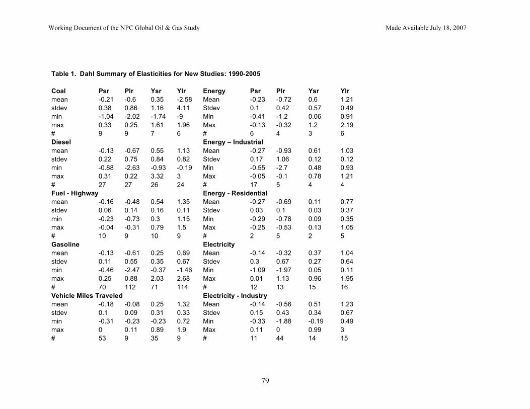
Working Document of the NPC Global Oil & Gas Study Made Available July 18, 2007
79
Table 1. Dahl Summary of Elasticities for New Studies: 1990-2005 Coal Psr Plr Ysr Ylr Energy Psr Plr Ysr Ylr mean -0.21 -0.6 0.35 -2.58 Mean -0.23 -0.72 0.6 1.21 stdev 0.38 0.86 1.16 4.11 Stdev 0.1 0.42 0.57 0.49 min -1.04 -2.02 -1.74 -9 Min -0.41 -1.2 0.06 0.91 max 0.33 0.25 1.61 1.96 Max -0.13 -0.32 1.2 2.19 # 9 9 7 6 # 6 4 3 6 Diesel Energy – Industrial mean -0.13 -0.67 0.55 1.13 Mean -0.27 -0.93 0.61 1.03 stdev 0.22 0.75 0.84 0.82 Stdev 0.17 1.06 0.12 0.12 min -0.88 -2.63 -0.93 -0.19 Min -0.55 -2.7 0.48 0.93 max 0.31 0.22 3.32 3 Max -0.05 -0.1 0.78 1.21 # 27 27 26 24 # 17 5 4 4 Fuel - Highway Energy - Residential mean -0.16 -0.48 0.54 1.35 Mean -0.27 -0.69 0.11 0.77 stdev 0.06 0.14 0.16 0.11 Stdev 0.03 0.1 0.03 0.37 min -0.23 -0.73 0.3 1.15 Min -0.29 -0.78 0.09 0.35 max -0.04 -0.31 0.79 1.5 Max -0.25 -0.53 0.13 1.05 # 10 9 10 9 # 2 5 2 5 Gasoline Electricity mean -0.13 -0.61 0.25 0.69 Mean -0.14 -0.32 0.37 1.04 stdev 0.11 0.55 0.35 0.67 Stdev 0.3 0.67 0.27 0.64 min -0.46 -2.47 -0.37 -1.46 Min -1.09 -1.97 0.05 0.11 max 0.25 0.88 2.03 2.68 Max 0.01 1.13 0.96 1.95 # 70 112 71 114 # 12 13 15 16 Vehicle Miles Traveled Electricity - Industry mean -0.18 -0.08 0.25 1.32 Mean -0.14 -0.56 0.51 1.23 stdev 0.1 0.09 0.31 0.33 Stdev 0.15 0.43 0.34 0.67 min -0.31 -0.23 -0.23 0.72 Min -0.33 -1.88 -0.19 0.49 max 0 0.11 0.89 1.9 Max 0.11 0 0.99 3 # 53 9 35 9 # 11 44 14 15
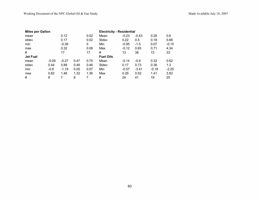
Working Document of the NPC Global Oil & Gas Study Made Available July 18, 2007
80
Miles per Gallon Electricity - Residential mean 0.12 0.02 Mean -0.23 -0.43 0.28 0.6 stdev 0.17 0.02 Stdev 0.22 0.5 0.18 0.88 min -0.36 0 Min -0.95 -1.5 0.07 -0.15 max 0.32 0.08 Max -0.12 0.65 0.71 4.34 # 17 17 # 13 38 13 33 Jet Fuel Fuel Oils mean -0.09 -0.27 0.47 0.75 Mean -0.14 -0.9 0.32 0.62 stdev 0.44 0.88 0.46 0.46 Stdev 0.17 0.73 0.38 1.3 min -0.8 -1.19 0.05 0.07 Min -0.57 -3.41 -0.18 -2.25 max 0.82 1.46 1.32 1.36 Max 0.29 0.02 1.41 3.83 # 8 7 8 7 # 24 41 19 25
Working Document of the NPC Global Oil & Gas Study Made Available July 18, 2007
81
Elasticities over Time None of the elasticities described to this point are anchored to an unwavering assumption that the future is necessarily identical to the past. Indeed, the magnitudes of all elasticities are influenced by changes technology, consumer preferences, beliefs and habits. They could also be changed by policies. For greater insights it is also useful to see how those elasticities might change over time. The figure on the following page illustrates this point. Using data from the EIA’s 2005 Annual Energy Review (AER 2005), Laitner (2006) updated a series of long-run price and income elasticities for total primary energy consumption in the United States. These elasticities are based on GDP (in 2000 dollars) and average energy prices (total expenditures divided by total primary energy consumption adjusted for the CPI-U in 1982-84 dollars) for the period 1970 through 2002. This is the latest year for which the Energy Information Administration (EIA) has publicly available data on energy expenditures. As shown in the chart below, the long-run income elasticities rise steadily while the (absolute value of) long-run price elasticities show considerably more volatility, peaking in the early 1980s and declining steadily since then. As other analysts have suggested elsewhere, income matters more than price, and policies which seek a balance between both energy efficiency and energy supply should reflect that point.
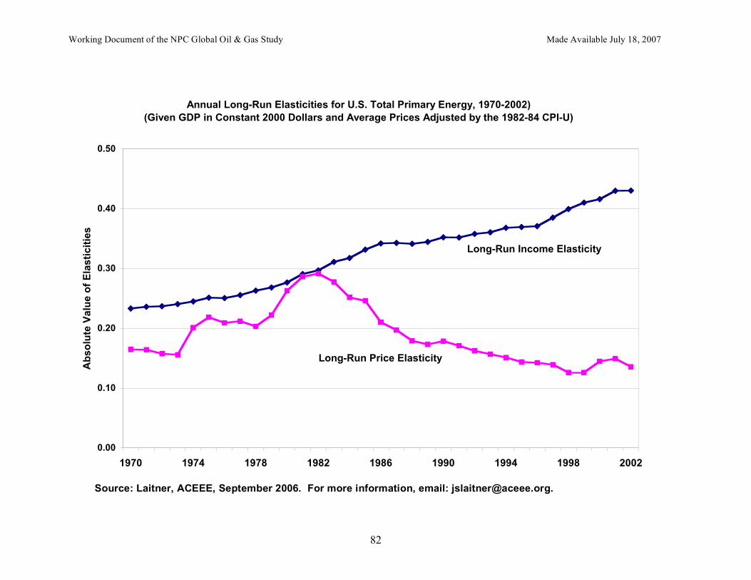
Working Document of the NPC Global Oil & Gas Study Made Available July 18, 2007
82
Annual Long-Run Elasticities for U.S. Total Primary Energy, 1970-2002)
(Given GDP in Constant 2000 Dollars and Average Prices Adjusted by the 1982-84 CPI-U)
0.00
0.10
0.20
0.30
0.40
0.50
1970 1974 1978 1982 1986 1990 1994 1998 2002
Ab
so
lute
Va
lue
of
Ela
sti
cit
ies
Long-Run Income Elasticity
Long-Run Price Elasticity
Source: Laitner, ACEEE, September 2006. For more information, email: [email protected].
Working Document of the NPC Global Oil & Gas Study Made Available July 18, 2007
83
Policy Insights Based on the available evidence, several policy insights emerge which are discussed below. 1. Income is more critical than price with respect to demand for energy. If policies focus only on rising price signals without providing alternatives to continued patterns, consumers and businesses may view those policies as more punitive than productive. On the other hand, policies which enable the adoption of more energy efficient technologies or which provide incentives to encourage greater energy efficiencies may be useful complements to price signals. 2. There are regional variations that may affect programs or policies that promote greater improvements in energy efficiency. 3. While there is evidence of significant reduction in the short run elasticities for gasoline, the evidence suggests that long term responsiveness to both price and policy signals may still be significant. 4. Price elasticities could be different when real prices are increasing (e.g., in last couple years), especially if real prices increase relative to real incomes. Most analyses are based on years when prices were decreasing relative to incomes. 5. Elasticities vary significantly over time suggesting that optimal policies may also need to vary in response to the capacity of consumers and businesses to adapt to changing market conditions. References Azevedo, Inês M. L. (2006) Bernstein, Mark A. and James Griffin (2005) Dahl, Carol (2006) Energy Information Administration (2006) Hughes, Jonathan E., Christopher R. Knittel, and Daniel Sperling (2006) International Energy Agency (2006) Laitner, John A. “Skip” (2006) Romani, Mattia, Orestes Soldatos, and Arthur van Benthem (2006)
Working Document of the NPC Global Oil & Gas Study Made Available July 18, 2007
84
Fuel Switching Trends Leads: Marianne Kah and Helen Currie (Conoco-Philips)
Introduction The ability to substitute fuels in a given sector impacts how vulnerable the sector is to supply disruptions and associated price spikes. The ability to substitute fuels during a disruption lessens demand for the disrupted fuel, thereby reducing the size of the shortfall and the associated price spike. Lacking the ability to substitute fuels, prices need to rise to fairly high levels in times of shortage in order to reduce the activity that is generating the demand for fuel. Why Energy Supply Disruptions and Price Volatility are Relevant to the Economy Major oil supply disruptions can lead to global oil price shocks, which have adverse economic consequences. A disruption and resulting oil price shock would hurt the economy by: • Increasing the wealth transferred from consuming to producing nations because
imports become more expensive, • Reducing domestic production of goods and services as a consequence of lower oil
consumption, and • Reducing total domestic output because non-oil markets cannot adjust efficiently to
the higher price of oil.48 The first two categories of disruption costs may be anticipated and adjusted to by private agents. However, the disruption costs arising from non-oil markets not immediately and completely adjusting to the sudden jump in the oil price may not be fully accounted for by the private sector. Furthermore, these changes result in productivity declines and reductions in employment and output.49 This large public cost of supply disruptions has been used in the past to justify government policies that lessen the impacts of a supply disruption (e.g., strategic petroleum reserves, IEA emergency oil sharing). Power blackouts in recent years, and damage inflicted by Hurricanes Katrina and Rita in the U.S. Gulf of Mexico in 2005 also demonstrate that domestic energy production and infrastructure are vulnerable to disruption. Energy supply security issues are much larger than imported oil.
In addition to major supply disruptions, prices in deregulated markets can be extremely volatile due to such supply and demand drivers as growth trends, weather, storage levels, and perceived market trends. Price volatility is a natural occurrence in mature, liquid, 48 Douglas R. Bohi & W. David Montgomery, “Oil Prices, Energy Security and Import Policy”, Resources for the Future Inc., 1982, page 91 49 Ibid., page 96
Working Document of the NPC Global Oil & Gas Study Made Available July 18, 2007
85
well functioning markets when new information is received by various market participants. Thus, the price level and volatility surrounding it reflect current information and expected future events relevant to the market. These price signals foster rational decision making by buyers and sellers and help steer the market towards an efficient allocation of resources. The private sector can also take action to mitigate price volatility. Consumers and producers have a broad range of physical and financial tools to mitigate the effects of price volatility if they so choose to bear the cost.
However, extreme price volatility has adverse consequences for consumers and manufacturers who have not been able to hedge the price of their energy supplies or do not otherwise have access to reasonably priced alternative fuels. For example, natural gas-intensive industries in the U.S., like the fertilizer industry, have needed to shut in capacity during periods of higher gas prices because the high feedstock cost made operations uneconomic. For other gas-intensive industries, like the petrochemicals industry, gas price spikes make it difficult for U.S. capacity to compete internationally since European and Asian competitors have oil-based feedstock.
High price volatility also hurts energy producers by increasing uncertainty and thereby raising their costs of capital. It could also reduce investment by increasing uncertainty around what the long-term equilibrium price will be. Extreme price volatility can be exacerbated by low elasticity of demand in the short-run. Demand can be inelastic in the short-term if there is a lack of alternative fuels to substitute. Given the adverse consequences of supply disruptions and extreme price volatility, there would be a benefit to increasing the ability of energy consumers to switch to alternative fuels. The remainder of this paper focuses on fuel-switching capability in the U.S. and other countries and what might be done to promote greater fuel-switching capability. The majority of the content focuses on the United States given the dearth of data in the rest of the world.
Working Document of the NPC Global Oil & Gas Study Made Available July 18, 2007
86
U.S. Fuel Switching and Flexibility a. U.S. Transportation Sector Fuel Switching and Flexibility Today there are only about 5 million light duty vehicles in the United States that have flexible fuel capability, representing about 2 percent of the total light duty fleet. About 13% of these flex-fuel vehicles are cars, and 87% are light trucks. The U.S. Department of Energy projects that by 2030 10% of new light duty vehicle sales will have E-85 flex fuel capability and an additional 1.3% will be CNG or LPG bi-fuel capable. By 2030, DOE projects that flexible fuel vehicle stocks account for 31 million vehicles or 7.7% of the light vehicle stock. LPG and CNG bi-fuel vehicles account for 1.3 million vehicles or 1.2% of the light vehicle stock. There is some fuel-switching capability in the U.S. based on the ability to blend more ethanol into gasoline. Given that ethanol production is rising at a faster rate than federal ethanol mandates, there will be additional capacity to use more ethanol if its price is below other high octane components for conventional gasoline. The ability to blend more ethanol would be helpful during an oil supply disruption. As long as the ethanol blend isn’t greater than 10 percent, existing vehicles and distribution systems can be utilized. On the other hand, an 85% blend would require flex-fuel vehicles and substantial investments in the distribution system. Today, there are 1000 filling stations in the U.S. that offer 29 million gallons of E-85, and that number is expected to grow as more flex-fuel vehicles are sold. However, E-85 growth will be limited until ethanol can be sourced by second generation feedstock that is not used for food. Consumers also need to be made aware of the 25 percent loss in fuel efficiency of E-85 versus conventional gasoline. In addition, automobile manufacturers need to insure that E-85 won’t adversely impact the durability of the vehicle. The fuels industry needs to make sure E-85 fuel specifications are updated. There are concerns about durability in terms of engine and fuel system deposits that could over time compromise drivability if specifications for ethanol sulfates, for example, are not updated. The volatility specifications for E-85 are also outdated and cannot be routinely met with market available components and blending constraints. The problem with not having a substantial volume of fuel substitution capability is that it leaves consumers exposed to price spikes during periods of market tightness. The price spikes could be minimized if there were substitute fuels that could be made available. While the prices of many fuel sources are correlated with oil prices, the correlation is not perfect, and thus the ability to use another fuel will directly help the consumer minimize price volatility. The availability of substitutes to oil will also help reduce oil price volatility since demand for oil can quickly be reduced during oil supply disruptions. Substitute fuel capacity will only help if there is excess capacity to produce the alternative fuel. Substantial excess capacity in an industry likely results in weak profitability and reduced investment. This issue would need to be dealt with to have real
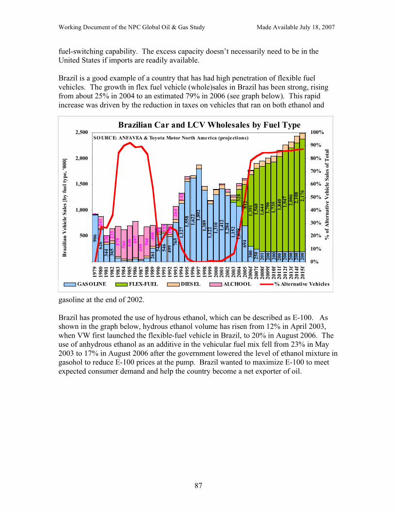
Working Document of the NPC Global Oil & Gas Study Made Available July 18, 2007
87
fuel-switching capability. The excess capacity doesn’t necessarily need to be in the United States if imports are readily available. Brazil is a good example of a country that has had high penetration of flexible fuel vehicles. The growth in flex fuel vehicle (whole)sales in Brazil has been strong, rising from about 25% in 2004 to an estimated 79% in 2006 (see graph below). This rapid increase was driven by the reduction in taxes on vehicles that ran on both ethanol and
gasoline at the end of 2002.
Brazil has promoted the use of hydrous ethanol, which can be described as E-100. As shown in the graph below, hydrous ethanol volume has risen from 12% in April 2003, when VW first launched the flexible-fuel vehicle in Brazil, to 20% in August 2006. The use of anhydrous ethanol as an additive in the vehicular fuel mix fell from 23% in May 2003 to 17% in August 2006 after the government lowered the level of ethanol mixture in gasohol to reduce E-100 prices at the pump. Brazil wanted to maximize E-100 to meet expected consumer demand and help the country become a net exporter of oil.
90
6 6
26
34
4 3
65
26
1 54
3
54
6 4
99 7
65 1
,12
7 1,5
58
1,6
22
1,8
02
1,3
89
1,1
22
1,3
10
1,4
12
1,2
84
1,1
52
1,0
78
69
4
30
0 2
50
20
1
20
0
20
0 2
00
20
0
32
8
1,5
60
1,6
44
1,7
06
1,7
35
1,8
40
1,9
47
2,0
06
2,1
08
2,1
76
32
41
13
6 23
3
57
9
56
66
46 69
74
59 5
66 4
00
82 15
11
96
26
4
14
2
20
0
20
0 2
00
1,3
9181
2
500
1,000
1,500
2,000
2,500
19
79
19
80
19
81
19
82
19
83
19
84
19
85
19
86
19
87
19
88
19
89
19
90
19
91
19
92
19
93
19
94
19
95
19
96
19
97
19
98
19
99
20
00
20
01
20
02
20
03
20
04
20
05
20
06
f2
00
7f
20
08
f2
00
9f
20
10
f2
01
1f
20
12
f2
01
3f
20
14
f2
01
5f
0%
10%
20%
30%
40%
50%
60%
70%
80%
90%
100%
GASOLINE FLEX-FUEL DIESEL ALCHOOL % Alternative Vehicles
Bra
zili
an
Veh
icle
Sale
s [b
y f
uel
typ
e, '
000]
Brazilian Car and LCV Wholesales by Fuel Type
SO URCE: ANFAVEA & Toyota Motor North America (projections)
% o
f A
lter
nati
ve
Veh
icle
Sale
s of
Tota
l
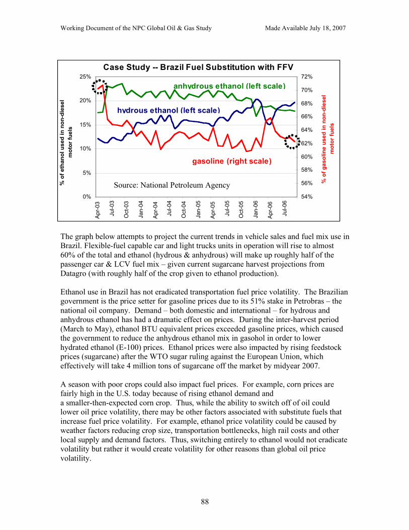
Working Document of the NPC Global Oil & Gas Study Made Available July 18, 2007
88
The graph below attempts to project the current trends in vehicle sales and fuel mix use in Brazil. Flexible-fuel capable car and light trucks units in operation will rise to almost 60% of the total and ethanol (hydrous & anhydrous) will make up roughly half of the passenger car & LCV fuel mix – given current sugarcane harvest projections from Datagro (with roughly half of the crop given to ethanol production). Ethanol use in Brazil has not eradicated transportation fuel price volatility. The Brazilian government is the price setter for gasoline prices due to its 51% stake in Petrobras – the national oil company. Demand – both domestic and international – for hydrous and anhydrous ethanol has had a dramatic effect on prices. During the inter-harvest period (March to May), ethanol BTU equivalent prices exceeded gasoline prices, which caused the government to reduce the anhydrous ethanol mix in gasohol in order to lower hydrated ethanol (E-100) prices. Ethanol prices were also impacted by rising feedstock prices (sugarcane) after the WTO sugar ruling against the European Union, which effectively will take 4 million tons of sugarcane off the market by midyear 2007. A season with poor crops could also impact fuel prices. For example, corn prices are fairly high in the U.S. today because of rising ethanol demand and a smaller-then-expected corn crop. Thus, while the ability to switch off of oil could lower oil price volatility, there may be other factors associated with substitute fuels that increase fuel price volatility. For example, ethanol price volatility could be caused by weather factors reducing crop size, transportation bottlenecks, high rail costs and other local supply and demand factors. Thus, switching entirely to ethanol would not eradicate volatility but rather it would create volatility for other reasons than global oil price volatility.
Case Study -- Brazil Fuel Substitution with FFV
0%
5%
10%
15%
20%
25%
Apr-03
Jul-03
Oct-03
Jan-04
Apr-04
Jul-04
Oct-04
Jan-05
Apr-05
Jul-05
Oct-05
Jan-06
Apr-06
Jul-06
% o
f e
tha
no
l u
se
d i
n n
on
-die
se
l
mo
tor
fuels
54%
56%
58%
60%
62%
64%
66%
68%
70%
72%
% o
f g
as
oli
ne
us
ed
in
no
n-d
ies
el
mo
tor
fuels
gasoline (right scale)
hydrous ethanol (left scale)
anhydrous ethanol (left scale)
Source: National Petroleum Agency
Working Document of the NPC Global Oil & Gas Study Made Available July 18, 2007
89
However, the ability to switch between fuels should allow the consumer to use whichever fuel has the lowest cost. This should reduce the volatility of fuel prices faced by consumers. It is important to note that outside of oil supply disruptions or periods of very tight oil supply/demand balances, ethanol costs have been significantly higher than conventional gasoline prices, particularly when adjusting for the lower energy content than conventional gasoline.
b. U.S. Power Sector Fuel Switching Power Generation appears to engage in short term fuel switching, especially during times of high natural gas prices. A 2002 EIA survey (reported in EEA report Natural Gas Issues for U.S. Power Generation, February 2004) reports that 36% (or 37.5 GW) of the 105 GW of power generation gas boilers had residual fuel oil as a 2nd fuel source. Between January 2000 and December 2002, 32% (33 GW) of the capacity used residual fuel oil at some time. The estimated gas equivalent of the fuel switching observed was ~8.5 BCF/D. Most the gas boiler capacity that used residual oil was in California, Florida, Illinois, Louisiana, Mississippi, New York and Texas. However, from CERA’s report Duel-fuel Steam Generation (November 2006), Texas and California have not demonstrated any fuel-switching capability. From the CERA report, the estimated demonstrated fuel switching capability ranges from 0.9 BCF/d to 1.5 BFC/d. The nameplate capacity for duel-fuel steam plants is reported as approximately 34 GW. CERA estimates 9 BCF/d of switching capability based on an estimated heat rate of 10,800 btu per kWh. Since the duel-fuel plants have been shown to be high on the dispatch stack for power generation (average utilization of ~26%) , the estimate peak is ~1.5 BCF/d. Most of this fuel switching capability is in the Northeast and the South. New York, Florida, Mississippi, and Louisiana are the states with the most fuel switching capability. The graph below illustrates that demand for natural gas for power generation is sensitive to relative prices. As the oil-to-gas price ratio increases (i.e., gas becomes cheaper relative to oil), natural gas consumption also increases. When the ratio falls, so does natural gas consumption. From this graph, there is a strong indication that there has been short term fuel switching from oil to gas as the price ratio between the two fuels moves.
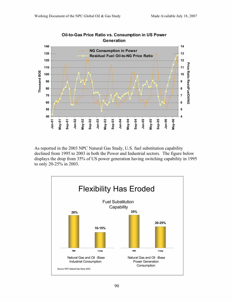
Working Document of the NPC Global Oil & Gas Study Made Available July 18, 2007
90
Oil-to-Gas Price Ratio vs. Consumption in US Power
Generation
40
50
60
70
80
90
100
110
120
130
140
Ja
n-0
1
Ma
y-0
1
Se
p-0
1
Ja
n-0
2
Ma
y-0
2
Se
p-0
2
Ja
n-0
3
Ma
y-0
3
Se
p-0
3
Ja
n-0
4
Ma
y-0
4
Se
p-0
4
Ja
n-0
5
Ma
y-0
5
Se
p-0
5
Ja
n-0
6
Ma
y-0
6
Th
ou
san
d B
OE
4
5
6
7
8
9
10
11
12
13
14P
rice R
atio
Resid
Fu
elO
il/NG
NG Consumption in Power
Residual Fuel Oil-to-NG Price Ratio
As reported in the 2003 NPC Natural Gas Study, U.S. fuel substitution capability declined from 1995 to 2003 in both the Power and Industrial sectors. The figure below displays the drop from 35% of US power generation having switching capability in 1995 to only 20-25% in 2003.
Flexibility Has Eroded
1995 Today
Fuel Substitution
Capability
1995 Today
26%
10-15%
35%
20-25%
Natural Gas and Oil -Base
Industrial Consumption
Natural Gas and Oil -Base
Power Generation
ConsumptionSource: NPC Natural Gas Study 2003
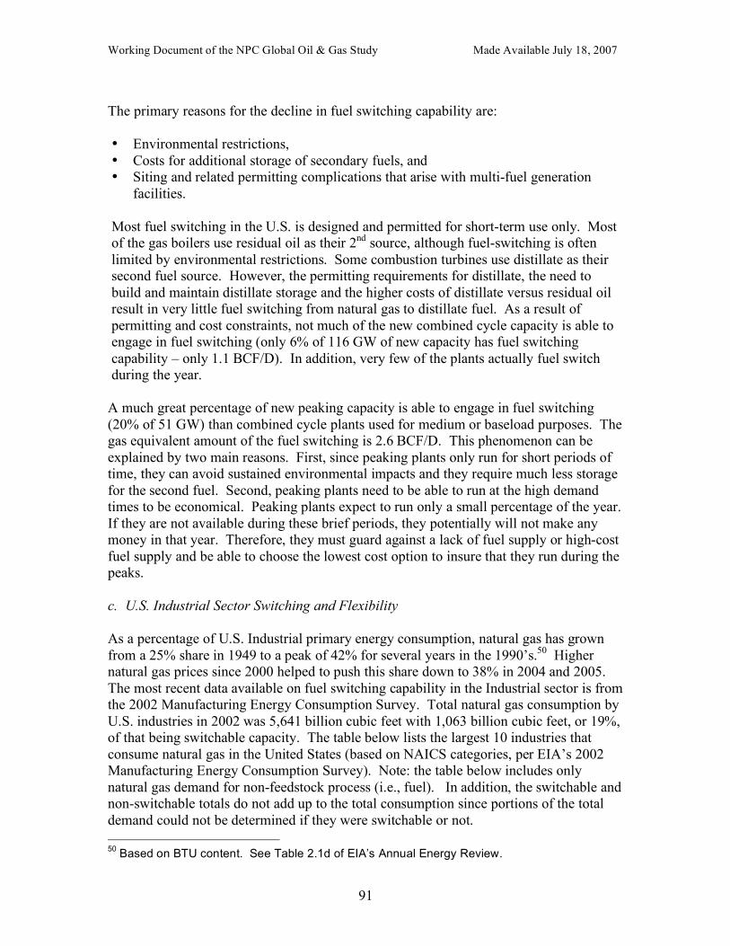
Working Document of the NPC Global Oil & Gas Study Made Available July 18, 2007
91
The primary reasons for the decline in fuel switching capability are: • Environmental restrictions, • Costs for additional storage of secondary fuels, and • Siting and related permitting complications that arise with multi-fuel generation
facilities. Most fuel switching in the U.S. is designed and permitted for short-term use only. Most of the gas boilers use residual oil as their 2nd source, although fuel-switching is often limited by environmental restrictions. Some combustion turbines use distillate as their second fuel source. However, the permitting requirements for distillate, the need to build and maintain distillate storage and the higher costs of distillate versus residual oil result in very little fuel switching from natural gas to distillate fuel. As a result of permitting and cost constraints, not much of the new combined cycle capacity is able to engage in fuel switching (only 6% of 116 GW of new capacity has fuel switching capability – only 1.1 BCF/D). In addition, very few of the plants actually fuel switch during the year.
A much great percentage of new peaking capacity is able to engage in fuel switching (20% of 51 GW) than combined cycle plants used for medium or baseload purposes. The gas equivalent amount of the fuel switching is 2.6 BCF/D. This phenomenon can be explained by two main reasons. First, since peaking plants only run for short periods of time, they can avoid sustained environmental impacts and they require much less storage for the second fuel. Second, peaking plants need to be able to run at the high demand times to be economical. Peaking plants expect to run only a small percentage of the year. If they are not available during these brief periods, they potentially will not make any money in that year. Therefore, they must guard against a lack of fuel supply or high-cost fuel supply and be able to choose the lowest cost option to insure that they run during the peaks. c. U.S. Industrial Sector Switching and Flexibility As a percentage of U.S. Industrial primary energy consumption, natural gas has grown from a 25% share in 1949 to a peak of 42% for several years in the 1990’s.50 Higher natural gas prices since 2000 helped to push this share down to 38% in 2004 and 2005. The most recent data available on fuel switching capability in the Industrial sector is from the 2002 Manufacturing Energy Consumption Survey. Total natural gas consumption by U.S. industries in 2002 was 5,641 billion cubic feet with 1,063 billion cubic feet, or 19%, of that being switchable capacity. The table below lists the largest 10 industries that consume natural gas in the United States (based on NAICS categories, per EIA’s 2002 Manufacturing Energy Consumption Survey). Note: the table below includes only natural gas demand for non-feedstock process (i.e., fuel). In addition, the switchable and non-switchable totals do not add up to the total consumption since portions of the total demand could not be determined if they were switchable or not. 50 Based on BTU content. See Table 2.1d of EIA’s Annual Energy Review.
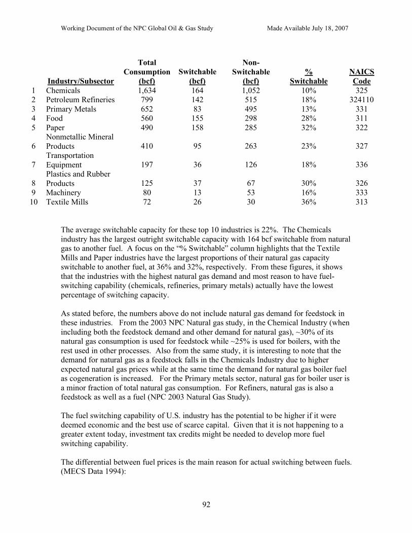
Working Document of the NPC Global Oil & Gas Study Made Available July 18, 2007
92
Industry/Subsector
Total Consumption
(bcf) Switchable
(bcf)
Non-Switchable
(bcf) %
Switchable NAICS Code
1 Chemicals 1,634 164 1,052 10% 325 2 Petroleum Refineries 799 142 515 18% 324110 3 Primary Metals 652 83 495 13% 331 4 Food 560 155 298 28% 311 5 Paper 490 158 285 32% 322
6 Nonmetallic Mineral Products 410 95 263 23% 327
7 Transportation Equipment 197 36 126 18% 336
8 Plastics and Rubber Products 125 37 67 30% 326
9 Machinery 80 13 53 16% 333 10 Textile Mills 72 26 30 36% 313
The average switchable capacity for these top 10 industries is 22%. The Chemicals industry has the largest outright switchable capacity with 164 bcf switchable from natural gas to another fuel. A focus on the “% Switchable” column highlights that the Textile Mills and Paper industries have the largest proportions of their natural gas capacity switchable to another fuel, at 36% and 32%, respectively. From these figures, it shows that the industries with the highest natural gas demand and most reason to have fuel-switching capability (chemicals, refineries, primary metals) actually have the lowest percentage of switching capacity. As stated before, the numbers above do not include natural gas demand for feedstock in these industries. From the 2003 NPC Natural gas study, in the Chemical Industry (when including both the feedstock demand and other demand for natural gas), ~30% of its natural gas consumption is used for feedstock while ~25% is used for boilers, with the rest used in other processes. Also from the same study, it is interesting to note that the demand for natural gas as a feedstock falls in the Chemicals Industry due to higher expected natural gas prices while at the same time the demand for natural gas boiler fuel as cogeneration is increased. For the Primary metals sector, natural gas for boiler user is a minor fraction of total natural gas consumption. For Refiners, natural gas is also a feedstock as well as a fuel (NPC 2003 Natural Gas Study). The fuel switching capability of U.S. industry has the potential to be higher if it were deemed economic and the best use of scarce capital. Given that it is not happening to a greater extent today, investment tax credits might be needed to develop more fuel switching capability. The differential between fuel prices is the main reason for actual switching between fuels. (MECS Data 1994):
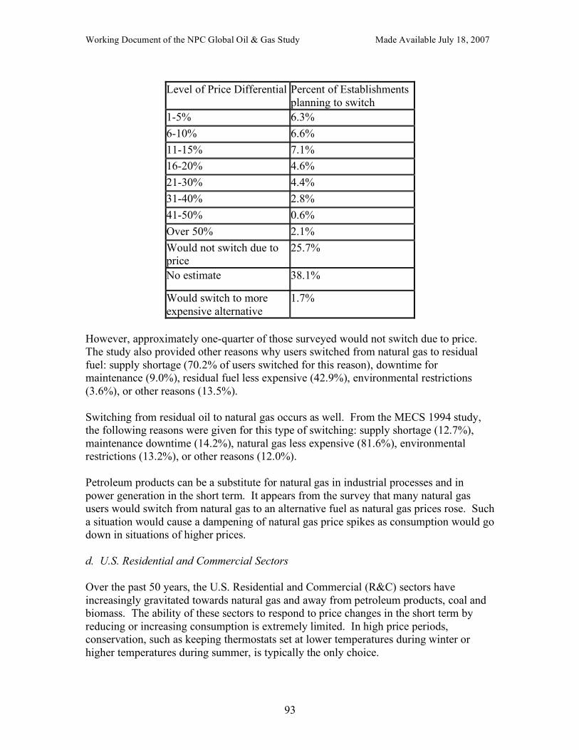
Working Document of the NPC Global Oil & Gas Study Made Available July 18, 2007
93
Level of Price Differential Percent of Establishments
planning to switch 1-5% 6.3% 6-10% 6.6% 11-15% 7.1% 16-20% 4.6% 21-30% 4.4% 31-40% 2.8% 41-50% 0.6% Over 50% 2.1% Would not switch due to price
25.7%
No estimate 38.1%
Would switch to more expensive alternative
1.7%
However, approximately one-quarter of those surveyed would not switch due to price. The study also provided other reasons why users switched from natural gas to residual fuel: supply shortage (70.2% of users switched for this reason), downtime for maintenance (9.0%), residual fuel less expensive (42.9%), environmental restrictions (3.6%), or other reasons (13.5%). Switching from residual oil to natural gas occurs as well. From the MECS 1994 study, the following reasons were given for this type of switching: supply shortage (12.7%), maintenance downtime (14.2%), natural gas less expensive (81.6%), environmental restrictions (13.2%), or other reasons (12.0%). Petroleum products can be a substitute for natural gas in industrial processes and in power generation in the short term. It appears from the survey that many natural gas users would switch from natural gas to an alternative fuel as natural gas prices rose. Such a situation would cause a dampening of natural gas price spikes as consumption would go down in situations of higher prices. d. U.S. Residential and Commercial Sectors Over the past 50 years, the U.S. Residential and Commercial (R&C) sectors have increasingly gravitated towards natural gas and away from petroleum products, coal and biomass. The ability of these sectors to respond to price changes in the short term by reducing or increasing consumption is extremely limited. In high price periods, conservation, such as keeping thermostats set at lower temperatures during winter or higher temperatures during summer, is typically the only choice.
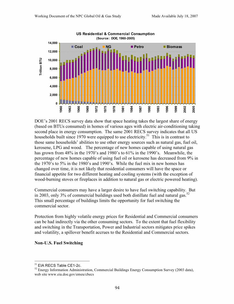
Working Document of the NPC Global Oil & Gas Study Made Available July 18, 2007
94
US Residential & Commercial Consumption (Source: DOE, 1960-2005)
0
2,000
4,000
6,000
8,000
10,000
12,000
14,000
1960
1963
1966
1969
1972
1975
1978
1981
1984
1987
1990
1993
1996
1999
2002
2005
Tri
llio
n B
TU
Coal NG Petro Biomass
DOE’s 2001 RECS survey data show that space heating takes the largest share of energy (based on BTUs consumed) in homes of various ages with electric air-conditioning taking second place in energy consumption. The same 2001 RECS survey indicates that all US households built since 1970 were equipped to use electricity.51 This is in contrast to those same households’ abilities to use other energy sources such as natural gas, fuel oil, kerosene, LPG and wood. The percentage of new homes capable of using natural gas has grown from 48% in the 1970’s and 1980’s to 61% in the 1990’s. Meanwhile, the percentage of new homes capable of using fuel oil or kerosene has decreased from 9% in the 1970’s to 5% in the 1980’s and 1990’s. While the fuel mix in new homes has changed over time, it is not likely that residential consumers will have the space or financial appetite for two different heating and cooling systems (with the exception of wood-burning stoves or fireplaces in addition to natural gas or electric powered heating). Commercial consumers may have a larger desire to have fuel switching capability. But in 2003, only 3% of commercial buildings used both distillate fuel and natural gas.52 This small percentage of buildings limits the opportunity for fuel switching the commercial sector. Protection from highly volatile energy prices for Residential and Commercial consumers can be had indirectly via the other consuming sectors. To the extent that fuel flexibility and switching in the Transportation, Power and Industrial sectors mitigates price spikes and volatility, a spillover benefit accrues to the Residential and Commercial sectors. Non-U.S. Fuel Switching
51 EIA RECS Table CE1-2c. 52 Energy Information Administration, Commercial Buildings Energy Consumption Survey (2003 data), web site www.eia.doe.gov/emeu/cbecs
Working Document of the NPC Global Oil & Gas Study Made Available July 18, 2007
95
European industrial and residential fuel switching capabilities at a single site are very low. In addition, there are few power plants in Europe that have dual fuel capabilities. Fuel switching in Europe generally occurs when large power companies, who own different types of power generation plants, run the plants that have the lowest cost fuels. In essence, fuel switching is not observed at a single plant, but rather over a portfolio of plants. For the Far East, no data was readily available for this study. Summary Fuel switching capability in the United States seems to be more developed than the capability in Europe. Given the short time fuse of this study, data on Asian fuel switching capability was not available. In the Transportation sector, flexible fueled vehicles enable the consumer to choose the lowest cost fuel, thereby providing some insulation from price spikes in any one fuel source. There would have to be excess production capacity either domestically or from imported sources for the alternative fuel source for fuel switching to actually occur during an oil supply disruption. The United States has some fuel-switching capability due to the ability to blend more ethanol into gasoline. Brazil serves as the best example of a country with a high penetration of flexible fuel vehicles where the growth in demand for flex-fuel vehicles was spurred by favorable tax treatment. Consumers can be somewhat protected from price shocks in one fuel if a significant portion of the vehicle fleet can run on multiple fuels. In the Power sector, government permitting and tax policies and construction costs are major influencers of fuel switching capacity, and neither favors building flexible fuel facilities today. Facilities that can utilize multiple fuels tend to require more storage space for those fuels. This larger footprint can pose problems with siting the facility. It is not unusual for there to be local opposition to the size of the facility or to other aspects such as additional access roads and truck traffic that may be associated with having fuel flexibility. Without the appropriate economic incentives and more favorable government policies (at local, state and national levels), consumers could face rolling blackouts or forced outages when peak demand exceeds short term baseload generation capacity. In the Industrial sector, the United States has some short-term fuel switching capability as shown in past studies but it has diminished over time. Surveys of major consumers reveal that fuel switching occurs in response to short term price dynamics or logistical constraints, with prices being the primary reason for fuel switching. The gas-intensive industries would most likely garner greatest benefit from having fuel flexibility in their operations but cannot do so primarily because gas is used as a feedstock as well as a fuel. The alternatives for fuel switching in the Residential and Commercial sectors are somewhat limited as natural gas has grown to be the single dominant energy source consumed. Protection from highly volatile energy prices for Residential and Commercial
Working Document of the NPC Global Oil & Gas Study Made Available July 18, 2007
96
consumers can be had indirectly via the other consuming sectors. To the extent that fuel flexibility and switching in the Transportation, Power and Industrial sectors mitigates price spikes and volatility, a spillover benefit accrues to the Residential and Commercial sectors. Policy Recommendations
Given the impact that a lack of fuel-switching capability has on energy security and associated price volatility, government policies should:
• Use tax credits to provide incentives to invest in dual-fuel capability in the industrial and power sectors
• Avoid policies that prevent fuel switching during supply disruptions. For example, governments should adopt emissions regulations that promote customer alternate fuel options and switchability (particularly for new power plant installations) during supply disruptions. Presently emissions regulations are limited fuel switching in the power and industrial sectors.
• Promote free market solutions to market issues.
– Let market signals tell the private sector when to switch
Private market participants can respond to price signals faster than the government. Thus, they are in a better position to decide when to switch then the government
– Avoid regulations or behavior that provides disincentives to fuel-switching


![Cultural Heritage and Technology. 10 Upcoming Trends. [ENG]](https://img.pdfslide.us/doc/110x75/587d56ee1a28abee158b5c73/cultural-heritage-and-technology-10-upcoming-trends-eng.jpg)