Embed Size (px)
Citation preview
BUSINESS
SCHOOL
Topic Seven: Risk and Return
Evelyn Lai

This lecture
› In this lecture, we will cover the following:
- Calculate realised and expected rates of return and risk for
individual assets
- Calculate the risk and return of portfolios
- Examine the components of total risk
›Readings: BMA Chapter 7

BUSINESS
SCHOOL
Risk and Return Calculations
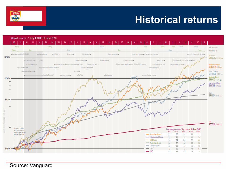
Historical returns
Source: Vanguard

Realised returns
› Realised return or cash return measures the gain or loss on
an investment.
11 )( ReturnCash
Stream IncomeGain CapitalReturnCash
ttt DivPP

Rate of return
› The rate of return is simply the cash return divided by the
beginning asset price.
t
ttt
t
tttt
P
DivP R
P
Div)P(P R
111
111
ln
Yield DividendYieldGain CapitalReturn of Rate
Price inningReturn/BegCash Return of Rate

Example
You invested in 1 share of Macquarie Group (MQG)
for $95 and sold a year later for $200. The company
did not pay any dividend during that period. What will
be the cash return on this investment? What is the
rate of return? How would these change if the
company paid a $10 dividend at the end of the
period?
_____________________________________________________
Rate of return

1. Expected return and risk – Historical time series
› Expected or mean return is what the investor expects to
earn from an investment in the future.
› The expected return is the arithmetic average of actual
returns over a specific period.
n
t
tn r
nn
rrrrrE
1
21 1)...()(
1. Expected return and risk – Historical time series
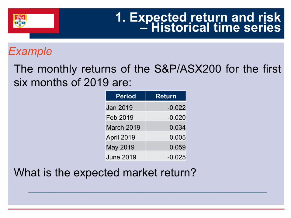
Example
The monthly returns of the S&P/ASX200 for the first
six months of 2019 are:
What is the expected market return?
_____________________________________________________
Period Return
Jan 2019 -0.022
Feb 2019 -0.020
March 2019 0.034
April 2019 0.005
May 2019 0.059
June 2019 -0.025
1. Expected return and risk – Historical time series
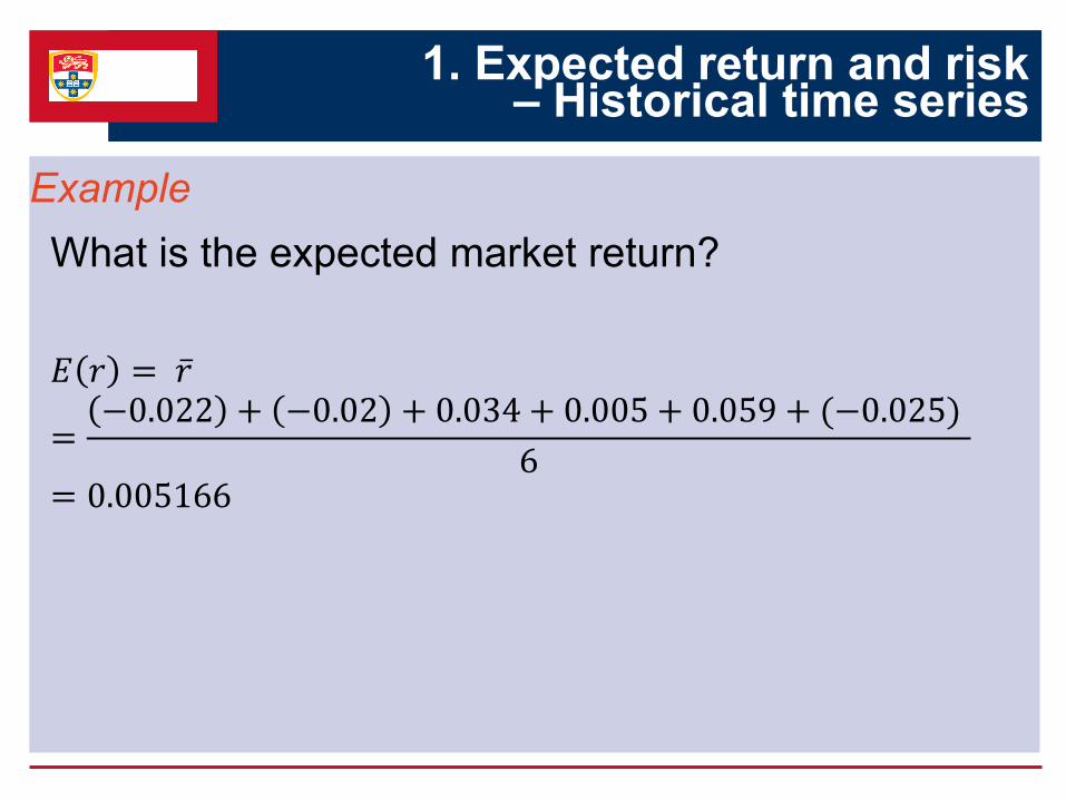
Example
What is the expected market return?
𝐸 𝑟 = 𝑟
=−0.022 + −0.02 + 0.034 + 0.005 + 0.059 + (−0.025)
6= 0.005166

Geometric vs arithmetic average rates of return
› The arithmetic average rate of return answers the question,
“What was the average of the rates of return per period?”
› The geometric or compound average rate of return answers
the question, “What was the growth rate of your investment?”
1. Expected return and risk – Historical time series
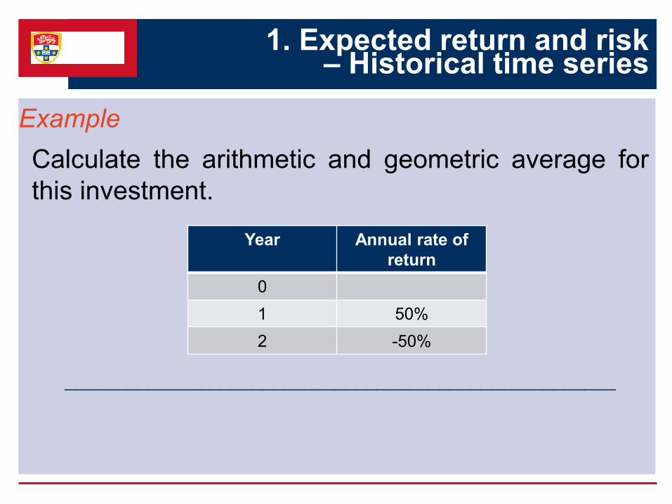
Example
Calculate the arithmetic and geometric average for
this investment.
_____________________________________________________
Year Annual rate of
return
0
1 50%
2 -50%

1. Expected return and risk – Historical time series
Example
I am considering investing in the S&P500 total returns index. I
would like to save $3 million over 30 years. How much would I
need to contribute each year to reach this goal? What
difference does arithmetic and geometric averages make?
_____________________________________________________2003 2004 2005 2006 2007 2008 2009 2010 2011 2012 2013 2014 2015 2016 2017 2018
S&P500 Total Returns 28.7 10.9 4.9 15.8 5.5 -37 -9.2 15.1 2.1 15.8 32.4 13.7 1.4 -22.1 -11.9 26.5
-40
-30
-20
-10
0
10
20
30
40
Retu
rns (
%)

1. Expected return and risk – Historical time series
› Total risk is the extent to which payoffs on an asset are
expected to vary from their average or expected value.
0%
10%
20%
30%
40%
50%
60%
70%
80%
90%
100%
-20.00%
-15.00%
-10.00%
-5.00%
0.00%
5.00%
10.00%
15.00%
20.00%
01-J
ul-9
2
01-F
eb
-93
01-S
ep
-93
01-A
pr-
94
01-N
ov-9
4
01-J
un-9
5
01-J
an-9
6
01-A
ug
-96
01-M
ar-
97
01-O
ct-
97
01-M
ay-9
8
01-D
ec-9
8
01-J
ul-9
9
01-F
eb
-00
01-S
ep
-00
01-A
pr-
01
01-N
ov-0
1
01-J
un-0
2
01-J
an-0
3
01-A
ug
-03
01-M
ar-
04
01-O
ct-
04
01-M
ay-0
5
01-D
ec-0
5
01-J
ul-0
6
01-F
eb
-07
01-S
ep
-07
01-A
pr-
08
01-N
ov-0
8
01-J
un-0
9
01-J
an-1
0
01-A
ug
-10
01-M
ar-
11
01-O
ct-
11
01-M
ay-1
2
01-D
ec-1
2
01-J
ul-1
3
01-F
eb
-14
01-S
ep
-14
01-A
pr-
15
01-N
ov-1
5
01-J
un-1
6
01-J
an-1
7
01-A
ug
-17
01-M
ar-
18
01-O
ct-
18
01-M
ay-1
9
Commonwealth Bank of Australia (CBA)
Monthly Returns Average Return (0.910%)
1. Expected return and risk – Historical time series
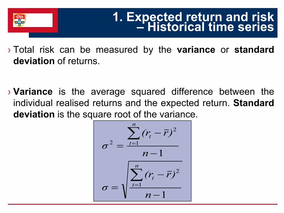
› Total risk can be measured by the variance or standard
deviation of returns.
› Variance is the average squared difference between the
individual realised returns and the expected return. Standard
deviation is the square root of the variance.
1
1
1
2
1
2
2
n
)r(r
σ
n
)r(r
σ
n
t
t
n
t
t

1. Expected return and risk – Historical time series
Example
The monthly returns of the S&P/ASX200 for the first
six months of 2019 are:
What is the risk of this market index?
_____________________________________________________
Period Return
Jan 2019 -0.022
Feb 2019 -0.020
March 2019 0.034
April 2019 0.005
May 2019 0.059
June 2019 -0.025
1. Expected return and risk – Historical time series
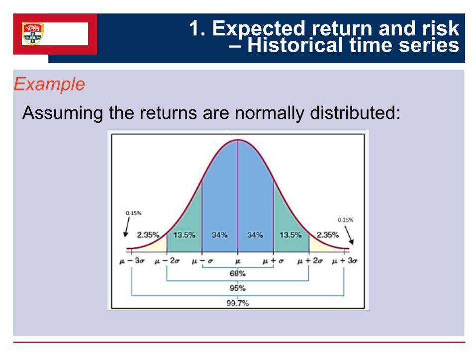
Example
Assuming the returns are normally distributed:
2. Expected return and risk – Probability distribution
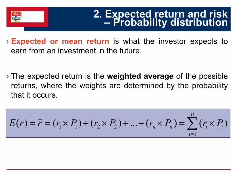
› Expected or mean return is what the investor expects to
earn from an investment in the future.
› The expected return is the weighted average of the possible
returns, where the weights are determined by the probability
that it occurs.
n
i
iinn PrPrPrPrrrE1
2211 )()(...)()()(
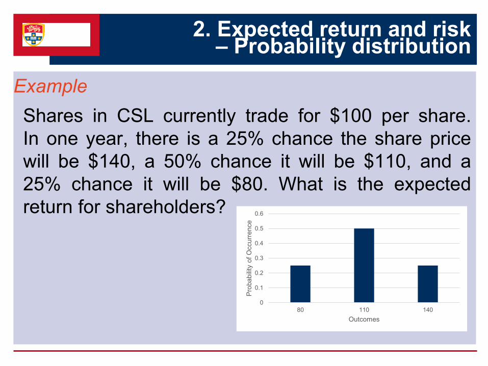
Example
Shares in CSL currently trade for $100 per share.
In one year, there is a 25% chance the share price
will be $140, a 50% chance it will be $110, and a
25% chance it will be $80. What is the expected
return for shareholders?
0
0.1
0.2
0.3
0.4
0.5
0.6
80 110 140
Pro
babili
ty o
f O
ccurr
ence
Outcomes
2. Expected return and risk – Probability distribution

2. Expected return and risk – Probability distribution
› When an investment is risky, there are different returns it may
earn. Each possible return has some likelihood of occurring.
This information is summarised with a probability distribution,
which assigns a probability that each possible return will
occur.
› The total risk is the weighted average of the possible returns,
where the weights are determined by the probability that it
occurs.
Pi
n
i
i rr 1
22

2. Expected return and risk – Probability distribution
› In finance, the standard deviation of a return is also referred
to as volatility. The standard deviation is easier to interpret
because it is in the same units as the returns themselves.
Pi
n
i
i rr 1
2

Example
Shares in CSL currently trade for $100 per share.
In one year, there is a 25% chance the share price
will be $140, a 50% chance it will be $110, and a
25% chance it will be $80. What is the variance of
returns?
0
0.1
0.2
0.3
0.4
0.5
0.6
80 110 140
Pro
babili
ty o
f O
ccurr
ence
Outcomes
2. Expected return and risk – Probability distribution
BUSINESS
SCHOOL
Risk and Return - Practical Application
A brief history of the financial markets
› Investors have historically earned higher rates of return on
riskier investments. However, having a higher expected rate of
return simply means that investors ‘expect’ to realise a higher
return. Higher return is not guaranteed.
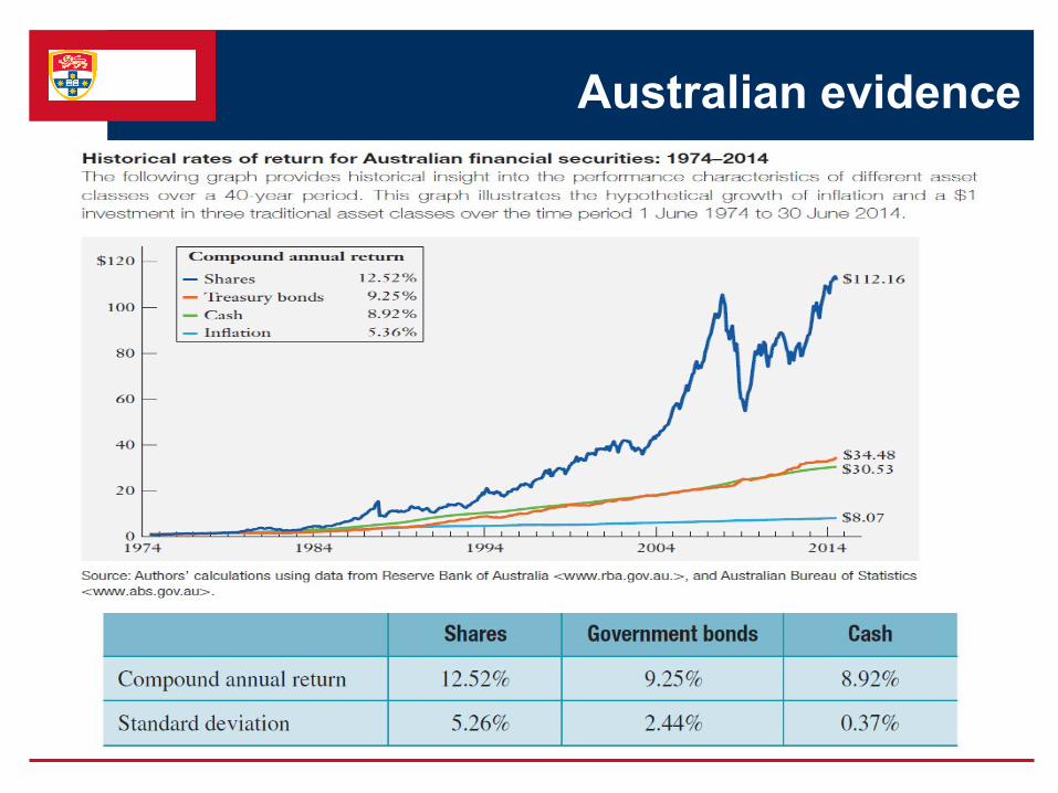
Australian evidence

US evidence
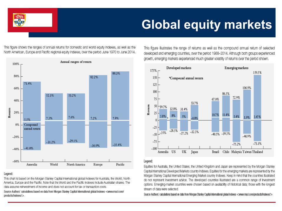
Global equity markets
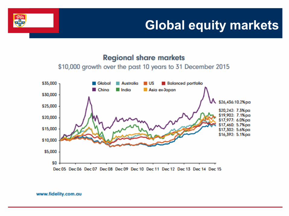
Global equity markets
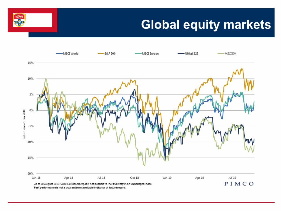
Global equity markets
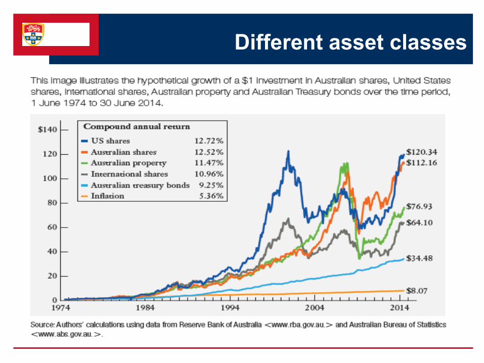
Different asset classes

BUSINESS
SCHOOL
Risk and Return of Portfolios

› A portfolio is a group of assets held by an investor.
› Holding a portfolio of assets reduces investment risk, but
often with no effect on overall returns, because:
- Within the portfolio, individual assets are more volatile than
the overall portfolio
- Poor returns on some assets could be offset by stronger
returns on others
- The overall portfolio return is “smoothed out”
Portfolios

› The portfolio expected return is a weighted average of the
expected returns on individual securities that make up the
portfolio, where weights correspond to the proportion of the
portfolio accounted by each of the respective component
assets.
𝐸 𝑟𝑝 = 𝑟𝑝 =
𝑖=1
𝑛
𝑤𝑖 𝐸(𝑟𝑖)
The return of portfolios
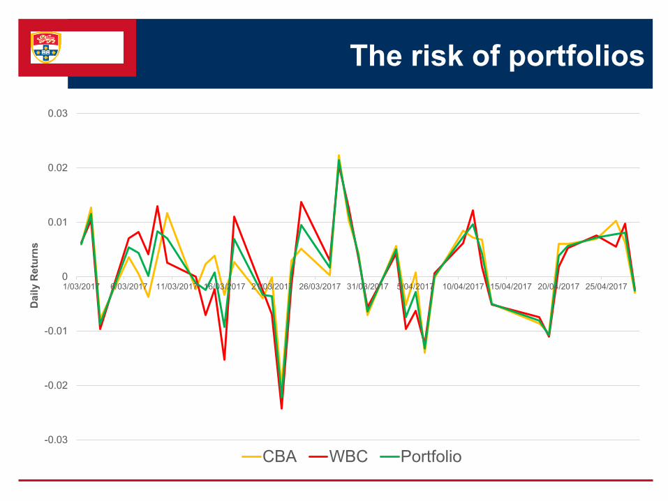
The risk of portfolios
-0.03
-0.02
-0.01
0
0.01
0.02
0.03
1/03/2017 6/03/2017 11/03/2017 16/03/2017 21/03/2017 26/03/2017 31/03/2017 5/04/2017 10/04/2017 15/04/2017 20/04/2017 25/04/2017
Da
ily R
etu
rns
CBA WBC Portfolio
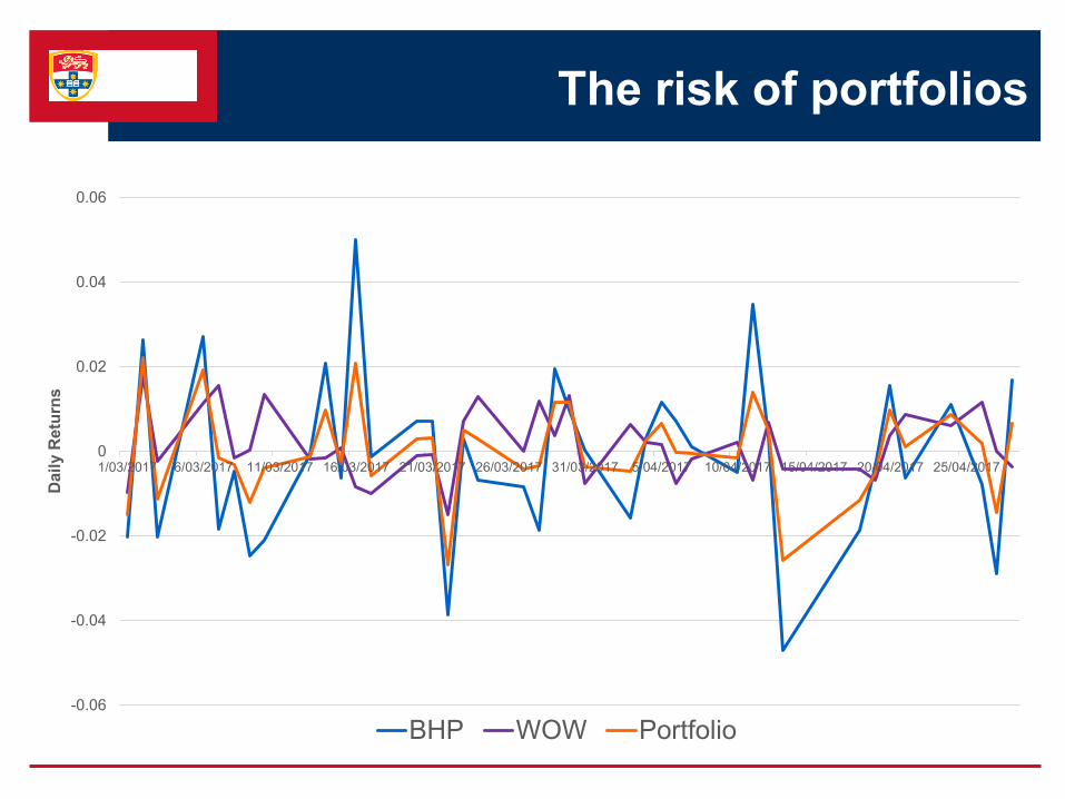
The risk of portfolios
-0.06
-0.04
-0.02
0
0.02
0.04
0.06
1/03/2017 6/03/2017 11/03/2017 16/03/2017 21/03/2017 26/03/2017 31/03/2017 5/04/2017 10/04/2017 15/04/2017 20/04/2017 25/04/2017
Da
ily R
etu
rns
BHP WOW Portfolio
The risk of portfolios
› The risk of a portfolio is measured by the variability or
dispersion of the portfolio return around its mean or expected
value.
› Unlike the expected return of a portfolio, risk of a portfolio is
not a simple weighted average of the risk of individual
security returns.
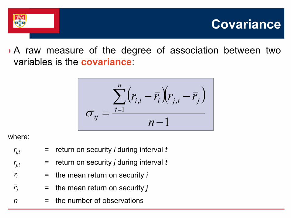
› A raw measure of the degree of association between two
variables is the covariance:
where:
ri,t = return on security i during interval t
rj,t = return on security j during interval t
= the mean return on security i
= the mean return on security j
n = the number of observations
1
1
,,
n
rrrrn
t
jtjiti
ij
jr
ir
Covariance
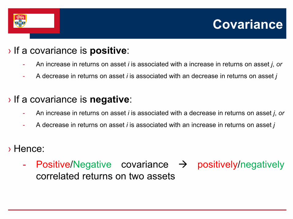
Covariance
› If a covariance is positive:
- An increase in returns on asset i is associated with a increase in returns on asset j, or
- A decrease in returns on asset i is associated with an decrease in returns on asset j
› If a covariance is negative:
- An increase in returns on asset i is associated with a decrease in returns on asset j, or
- A decrease in returns on asset i is associated with an increase in returns on asset j
› Hence:
- Positive/Negative covariance positively/negatively
correlated returns on two assets
Covariance
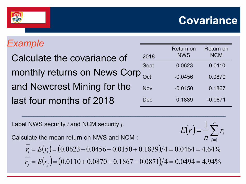
Example
Calculate the covariance of
monthly returns on News Corp
and Newcrest Mining for the
last four months of 2018
__________________________________________________________________________________________
Label NWS security i and NCM security j.
Calculate the mean return on NWS and NCM :
2018
Return on
NWS
Return on
NCM
Sept 0.0623 0.0110
Oct -0.0456 0.0870
Nov -0.0150 0.1867
Dec 0.1839 -0.0871
n
t
trn
rE1
1
%94.40494.040871.01867.00870.00110.0
%64.40464.041839.00150.00456.00623.0
jj
ii
rEr
rEr
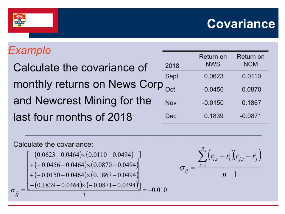
Covariance
Example
Calculate the covariance of
monthly returns on News Corp
and Newcrest Mining for the
last four months of 2018
__________________________________________________________________________________________
Calculate the covariance:
2018
Return on
NWS
Return on
NCM
Sept 0.0623 0.0110
Oct -0.0456 0.0870
Nov -0.0150 0.1867
Dec 0.1839 -0.0871
010.0
3
0494.00871.00464.01839.0
0494.01867.00464.00150.0
0494.00870.00464.00456.0
0494.00110.00464.00623.0
ij
1
1
,,
n
rrrrn
t
jtjiti
ij

Correlation coefficient
› An alternative, and closely related, measure of the degree of
association between two securities is the correlation
coefficient:
where:
σij = covariance between returns on securities i and j
σi = standard deviation of security i
σj = standard deviation of security j
ij ij
i j
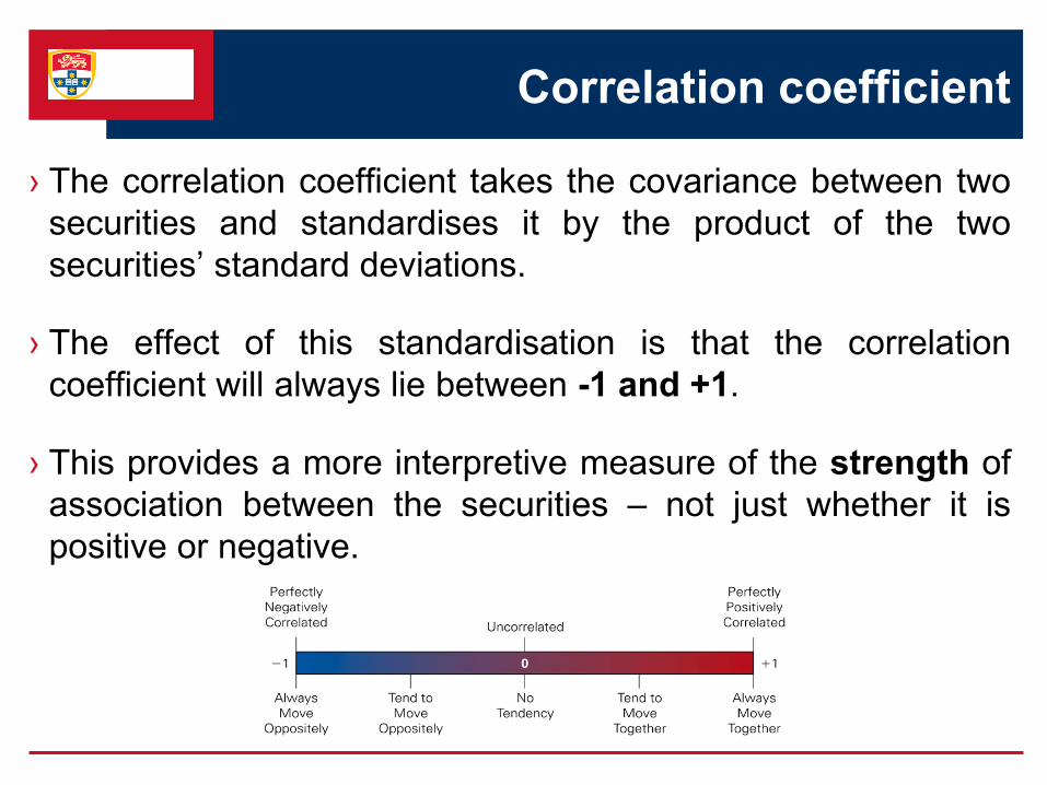
Correlation coefficient
› The correlation coefficient takes the covariance between two
securities and standardises it by the product of the two
securities’ standard deviations.
› The effect of this standardisation is that the correlation
coefficient will always lie between -1 and +1.
› This provides a more interpretive measure of the strength of
association between the securities – not just whether it is
positive or negative.

Correlation coefficient
Example
Calculate the correlation coefficient for News Corp
and Newcrest Mining, given that the standard
deviation of returns on the two stocks were 7.73%
and 11.59% and the covariance is –0.000656.
__________________________________________________
› 073.01159.00773.0
000656.0
ji
ij
ij

The risk of portfolios
› The risk of a portfolio is related to the riskiness of the
stocks and the degree of covariance or correlation.
› The variance of returns on a portfolio is calculated as follows:
where:
σi, σj = the standard deviation of returns on asset i or j
wi, wj = proportion of the portfolio invested in asset i or j
σij = the covariance between assets i and j
ρij = the correlation coefficient between assets i and j
jiijjijjiip
ijjijjiip
wwww
wwww
2
2
22222
22222
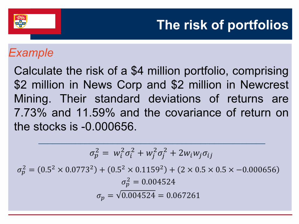
The risk of portfolios
Example
Calculate the risk of a $4 million portfolio, comprising
$2 million in News Corp and $2 million in Newcrest
Mining. Their standard deviations of returns are
7.73% and 11.59% and the covariance of return on
the stocks is -0.000656._________________________________________________
𝜎𝑝2 = 𝑤𝑖
2𝜎𝑖2 +𝑤𝑗
2𝜎𝑗2 + 2𝑤𝑖𝑤𝑗𝜎𝑖𝑗
𝜎𝑝2 = 0.52 × 0.07732 + 0.52 × 0.11592 + 2 × 0.5 × 0.5 × −0.000656
𝜎𝑝2 = 0.004524
𝜎𝑝 = 0.004524 = 0.067261
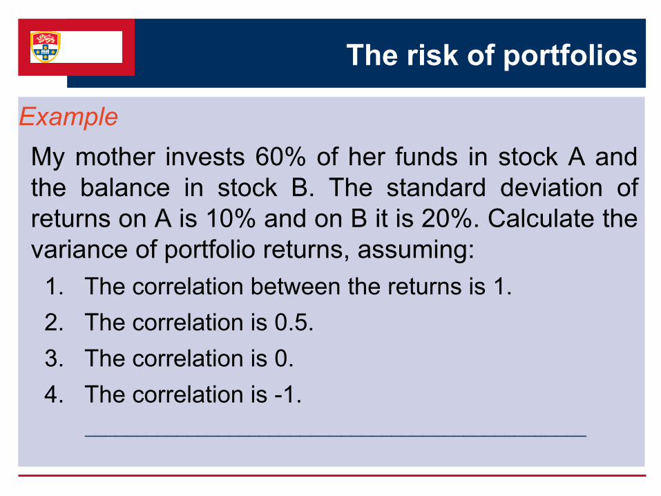
The risk of portfolios
Example
My mother invests 60% of her funds in stock A and
the balance in stock B. The standard deviation of
returns on A is 10% and on B it is 20%. Calculate the
variance of portfolio returns, assuming:
1. The correlation between the returns is 1.
2. The correlation is 0.5.
3. The correlation is 0.
4. The correlation is -1.
_________________________________________________

The risk of portfolios

The risk of portfolios
› The variance of returns on a three-asset portfolio is calculated
as follows:
› This can be extended to an n-asset case:
jkkjikkiijjikkjjiip wwwwwwwww 2222222222
ij
n
i
n
j
jip ww
1 1
2

Components of risk
› The risk of investing in a single security can be reduced by
combining the security with others in a portfolio due to
diversification.
› However, this does not mean that all risk can be eliminated.
› This is because there are two components of total risk:
1. Non-systematic (or diversifiable) risk
2. Systematic (or non-diversifiable) risk

› Non-systematic risk relates to price movements that are
caused by an event that influences a single company alone.
› It is also known as diversifiable risk because it can be
diversified away.
› Systematic risk relates to macroeconomic events that affect
the prices of all securities and are reflected in broad market
movements.
› It is referred to as ‘non-diversifiable’ as it is common to all
securities and cannot be diversified away.
Components of risk

Components of risk
0
5 10 15
Po
rtfo
lio
ris
k
Number of Securities
Market risk
Unique
risk
› Diversification eliminates the non-systematic risk of a
portfolio.
› A well-diversified portfolio faces market risk alone and the
level of market risk will depend on the market risk of individual
assets included in the portfolio.
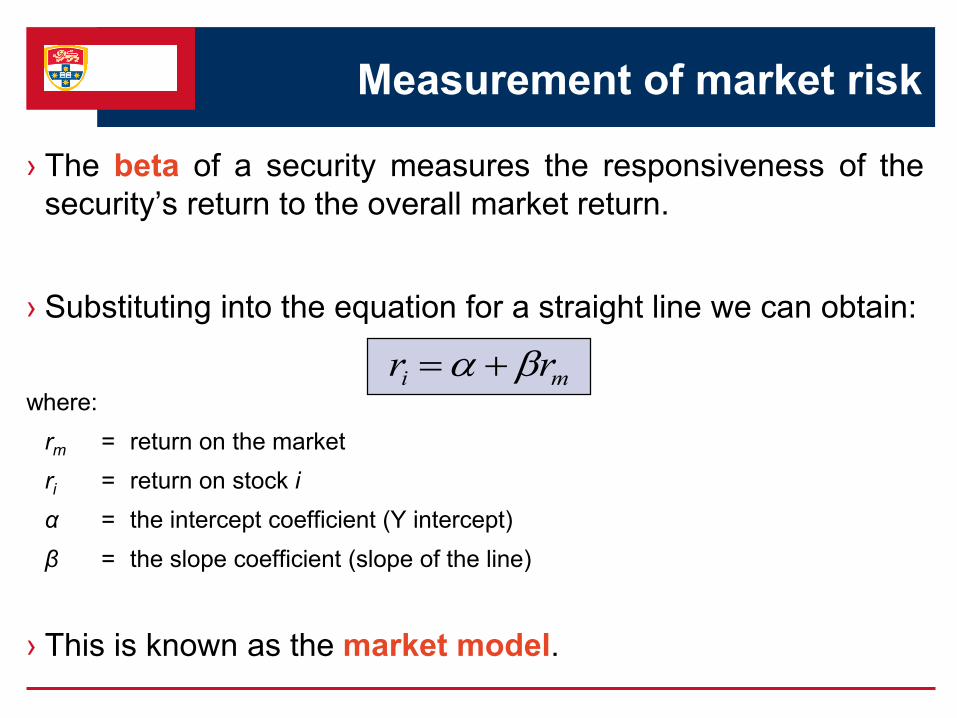
Measurement of market risk
› The beta of a security measures the responsiveness of the
security’s return to the overall market return.
› Substituting into the equation for a straight line we can obtain:
where:
rm = return on the market
ri = return on stock i
α = the intercept coefficient (Y intercept)
β = the slope coefficient (slope of the line)
› This is known as the market model.
ri rm
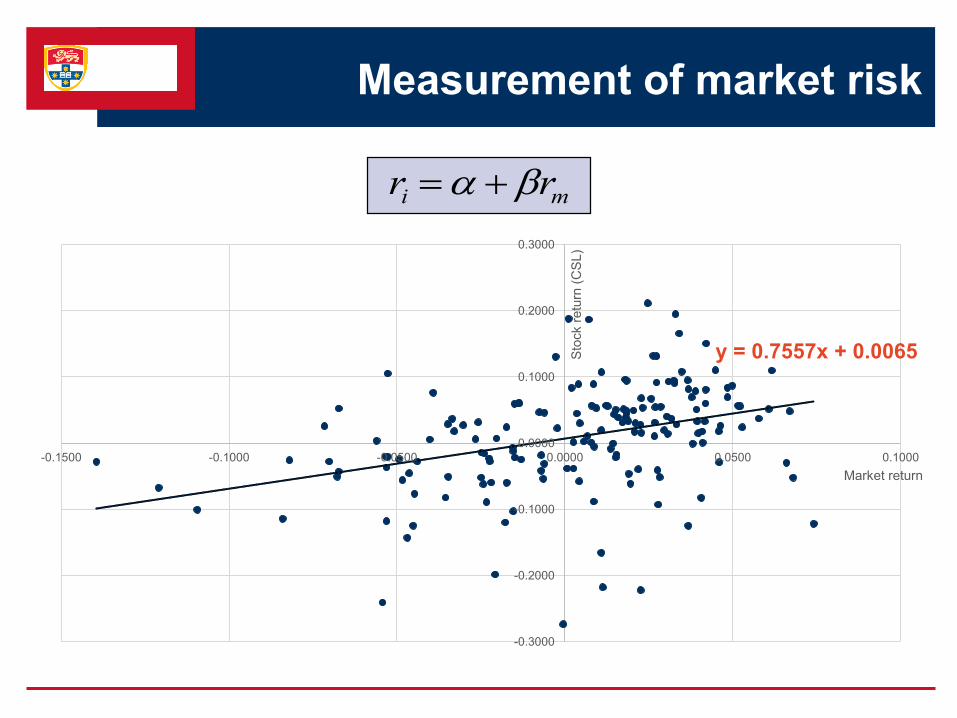
Measurement of market risk
ri rm
y = 0.7557x + 0.0065
-0.3000
-0.2000
-0.1000
0.0000
0.1000
0.2000
0.3000
-0.1500 -0.1000 -0.0500 0.0000 0.0500 0.1000
Sto
ck r
etu
rn (
CS
L)
Market return
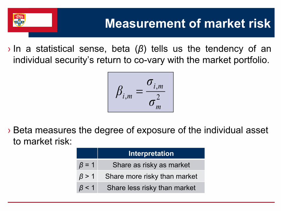
Measurement of market risk
› In a statistical sense, beta (β) tells us the tendency of an
individual security’s return to co-vary with the market portfolio.
› Beta measures the degree of exposure of the individual asset
to market risk:
Interpretation
β = 1 Share as risky as market
β > 1 Share more risky than market
β < 1 Share less risky than market
2
,
,
m
mi
miσ
σβ
Conclusion
› Calculation of realised returns.
› Calculation of expected returns.
1. Returns from a time series
2. Returns from a probability distribution
› Calculation of risk.
1. Returns from a time series
2. Returns from a probability distribution
› The risk and return of portfolios.
› The components of total risk (non-systematic and systematic).
›Next lecture: CAPM

BUSINESS
SCHOOL
The End