Topic 6. Product differentiation (I): patterns of price setting Economía Industrial Aplicada Juan Antonio Máñez Castillejo Departamento de Estructura Económica

Topic 6. Product differentiation (I): patterns of price setting

Economía Industrial AplicadaJuan Antonio Máñez Castillejo

Departamento de Estructura EconómicaUniversidad de Valencia

Departamento de Estructura Económica 2

Index

Topic 7. Product differentiation: patterns of

price setting

1. Introduction

2. Horizontal versus vertical product differentiation

3. The linear city model

3.1 Linear transport costs

3.2 Quadratic transport costs

4. Applications: Coca-Cola versus Pepsi-Cola

5. Conclussions


1. Introducción

Main implication of the homogeneous product assumption

in an oligopoly model of price competition (à la Bertrand)

• Bertrand paradox Price competition between two

firms is a sufficient condition to restores the

competitive situation p = c

Aim: To study an oligopoly model relaxing the

homogeneous product assumption, to analyse the effect

of product differentiation on price competition intensity

and product choice.


2. Horizontal and vertical product differentiation

Horizontal product differentiation: two products are

differentiated horizontally if, when they are offered at the

same price consumers do not agree on which is the

preferred product.Example: pine washing-up liquid and lemon-washing up liquid

Vertical product differentiation: two products are

differentiated vertically if, when they are offered at the same

price consumers agree on which is the preferred product.

• Example: washing-up liquid with and without product

moisturizing add-up.


Example

Opel Astra Ford Focus

Opel Corsa Ford Fiesta

Vertical Dif. Vertical Dif.

Horizontal Dif.

Horizontal Dif.


3.1 Linear city model with linear transport costs : assumptions

Two firms (firms 1 and 2) are located along the segment

The two firms sell a product that is identical except for the

location of the firm.

The two firms have constant and identical marginal cost c

c1=c2=c

Each consumer buys a single unit of the product.

Alternative interpretation of the segment as a product

characteristic

0 L

Consumers are uniformly distributed with unit density along a segment of L length


3.1 Linear city model with linear transport costs : two-stage game

Stage 1: the two firms choose simultaneously their location (long-run decision)

Stage 2: the two firms choose simultaneously their prices (short-run decision)We impose maximum product differentiation and so we focus on the determination of the Nash equilibrium in prices (Stage 2).

0 L

F1 F2


3.1 Linear city model with linear transport costs : consumers’ utility function

r: reservation price pj: price of the product of firm j

xij.: distance (along the segment) between the location of consumer i and the location of firm jt: transport cost per unit of distance (or alternatively intensity of the preference for a given product)

i j ijjU r p tx

The utility that a consumer i located in X obtains from the purchase of of the good of firm j is given by:


3.1 Linear city model with linear transport costs : transport costs

• Transport cost if the product is bought at firm 1 = tx• Transport cost if the product is bought at firm 2 = t(L-x)

Total cost of the product = price + transport costs

• Total cost if the product is bought at firm 1 = p1+ tx

• Total cost if the product is bought at firm 2= p2+ t(L-x)

With linear transport costs per unit of distance :

0 L

F1 F2

X

x L-x


3.1 Linear city model with linear transport costs : demands determination

d2=L-x

d1=x

X0 L

F1 F2

,1 ,2X XU U

1 2 ( )r p tx r p t L x

1 2p tx p t L x

2 1 1 21 22 2 2 2

p p L p p Ld x d L x

t t


3.1 Linear city model with linear transport costs : demand properties

Price elasticity of demand

1 1 1

1 1 2 1

0d p pp d p p Lt

1

22 1

0( )

Lpt p p Lt

Price elasticity of demand and transport costs


3.1 Linear city model with linear transport costs : demands determination

Total cost of buying at 1 = Total cost of buying at 2

1 2p tx p t L x

p1

d1d2

p2

1p tx

0 LxF1 F2

2p t L x

x0 x1

1 0p tx1 1p tx


3.1 Linear city model with linear transport costs : firm 1 demand

21d

21p

31d

31p

41d

41p

2p

F1

11p

11d

F20 L


Maximization problem of firm 1

Maximization problem of firm 2

1

2 11 1 1 1max

2 2p

p p Ld p c p c

t

1 2 1

1

2. . . 0

2 2d p p c L

F O Cdp t

* 2

1 2( ) 2

p Lt cp p Firm 1 reaction function

2

1 22 2 2 2max

2 2p

p p Ld p c p c

t

2 1 2

2

2. . . 0

2 2d p p c L

F O Cdp t

* 1

2 1( )2

p Lt cp p Firm 2 reaction function

3.1 Linear city model with linear transport costs : Obtaining the Nash equilibrium in prices (I)


Solving the system of equations given by the two reaction functions we obtain the price equilibrium: (given locations)

1 2c cp p Lt c

Profits for both firms are:

p*2(p1)

p*1(p2)

(Lt+c)/2

(Lt+c)/2

Lt+c

Lt+c

p2

p1

21 2

12

L t

3.1 Linear city model with linear transport costs : Obtaining the Nash equilibrium in prices (II)


Although both products are physically identical, as long as t>0 the price is greater than the marginal cost

p c Lt

Why?:• The larger is t the more differentiated are the products for

the consumers the higher is the costs of buying in a further shop.

• The larger is t the lower in the intensity of competition between firms 1 and 2 (for the consumers located between the two firms).

• When t=0 the products are not differentiated any more price is equal to marginal cost as in the Bertrand model with homogeneous.

3.1 Linear city model with linear transport costs : Obtaining the Nash equilibrium in prices (I)


Two extreme cases:• Maximum product differentiation: if t >0 p>c y >0• Minimum product differentiation: both firms choose the same location

no differentiation Bertrand model with homogeneous products

1 2 1 2 y 0c cp p c

p1

E1

p2

E2

p3

E1

E1 y E2

E1 y E2

p0

c

0 LF1 y F2

3.1 Linear city model with linear transport costs : Analysis of the location decisions (I)


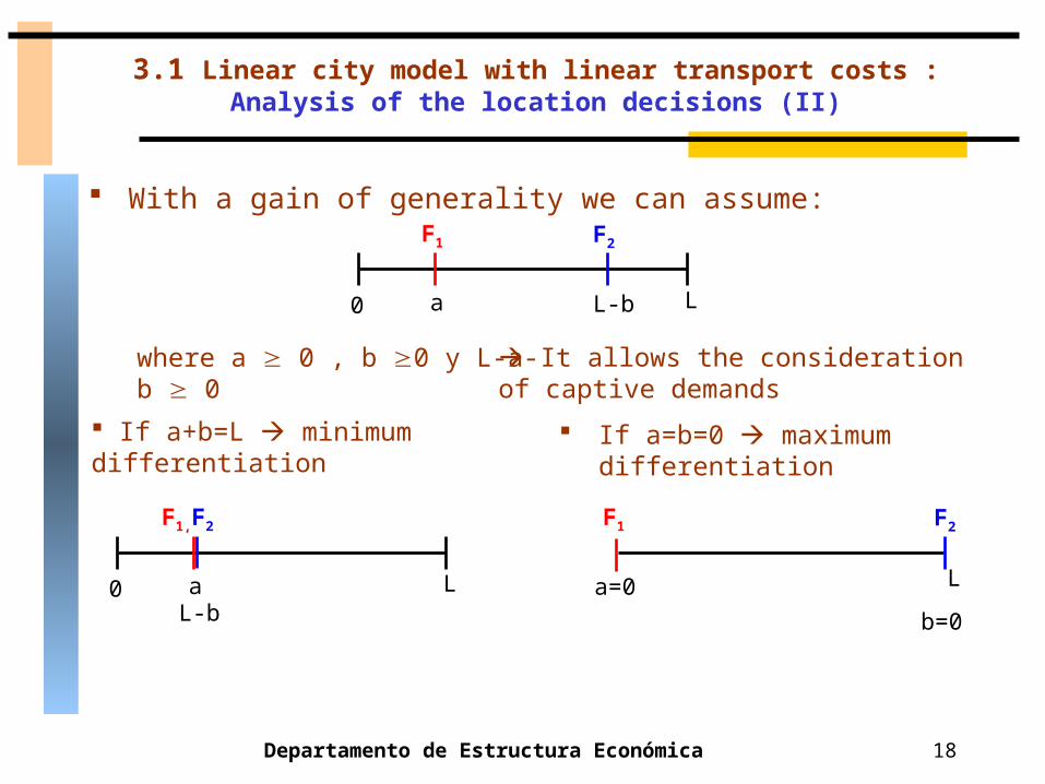
With a gain of generality we can assume:

L

If a=b=0 maximum differentiation

a=0

F1 F2

b=0

0 aL-b

L

F1,F2

If a+b=L minimum differentiation

3.1 Linear city model with linear transport costs : Analysis of the location decisions (II)

0 a L-b L

F1 F2

where a 0 , b 0 y L-a-b 0 It allows the consideration of captive demands


Nash equilibrium in locations is the one in which firm i (i=1,2) takes its optimal decision of location and price given its rival’s locations an price decisions

The original result in the Hottelling model (1929): minimum differentiation. Once prices have been chosen, both firms locate in the centre of the segment L/2

a’

1d'1d0

L

3.1 Linear city model with linear transport costs : Analysis of the location decisions (III)

cF1

a

1p

F2

L-b

2p

c


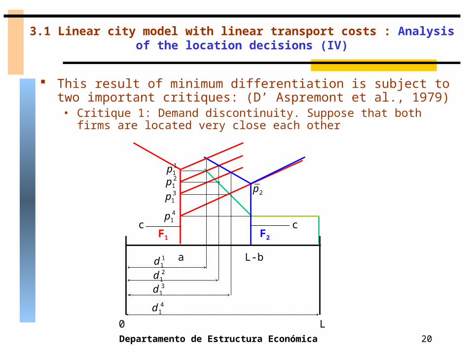
This result of minimum differentiation is subject to two important critiques: (D’ Aspremont et al., 1979)• Critique 1: Demand discontinuity. Suppose that both firms are

located very close each other

21p

21d

31p

31d

41p

41d

0 L

11d

3.1 Linear city model with linear transport costs : Analysis of the location decisions (IV)

L-b

F2

2p

c

a

F1

11p

c


Critique 2: Suppose that both firms are located at L/2 There is no product differentiation: each firm has an incentive

to undercut the price of the rival until p1=p2=c.

D’Aspremont et al. (1979) shows that que a=b=L/2 is not a Nash equilibrium in locations both firms have an incentive to deviate from L/2 to set a p>c y and in this way they would obtain positive profits

Price competition with homogeneous products

0 01 2p p c

a’

11d 1

2d

11pc

2a b L

0 L

1 2p p

3.1 Linear city model with linear transport costs : Analysis of the location decisions (V)


3.2 Linear city model with quadratic transport costs :Assumptions

It solves the problem of the inexistence of Nash equilibrium in locations that arises in the model with linear transport cost.

Differences with the linear transport costs model :

0 a L-b L

F1 F2

where a 0 , b 0 y L-a-b 0

• We do not impose maximum product differentiation to obtain the Nash

equilibrium in prices.

2

ij j ijU r p t x

• Utility function


With quadratic transport costs the umbrellas that represent the total cost of purchase are U-shaped.

11p

11d

21p

21d

L0L-b

2p

a

01p

c01d x

3.2 Linear city model with quadratic transport costs :Discontinuities in demand


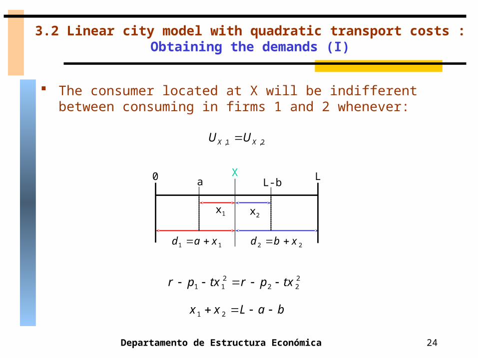
The consumer located at X will be indifferent between consuming in firms 1 and 2 whenever:

,1 ,2X XU U

1 1d a x 2 2d b x

x2x1

X0 a L-b L

2 21 1 2 2r p tx r p tx

3.2 Linear city model with quadratic transport costs :Obtaining the demands (I)

1 2x x L a b


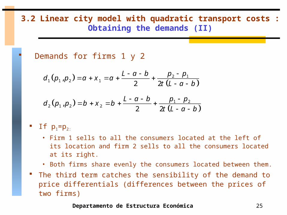
If p1=p2:

• Firm 1 sells to all the consumers located at the left of its location and firm 2 sells to all the consumers located at its right.

• Both firms share evenly the consumers located between them.

The third term catches the sensibility of the demand to price differentials (differences between the prices of two firms)

2 11 1 2 1,

2 2L a b p p

d p p a x at L a b

1 22 1 2 2,

2 2L a b p p

d p p b x bt L a b

Demands for firms 1 y 2

3.2 Linear city model with quadratic transport costs :Obtaining the demands (II)


Two-stage game:• Stage 1: Firms choose locations simultaneously.• Stage 2: Firms choose prices simultaneously.

We solve by backwards induction: each firm anticipates that its location decision affects not only its demand but also price competition intensity• To obtain the Nash equilibrium in prices given locations

(a,b).• To obtain the Nash equilibrium in locations given prices.

3.2 Linear city model with quadratic transport costs :Obtaining the equilibrium in prices and locations (II)


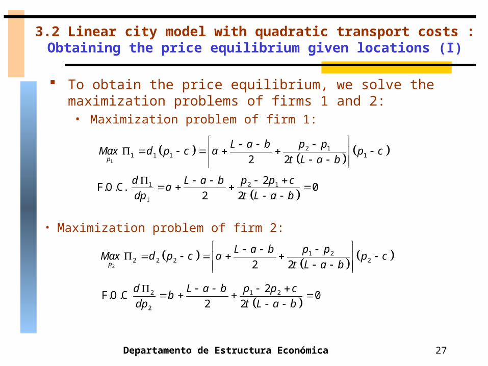
To obtain the price equilibrium, we solve the maximization problems of firms 1 and 2:• Maximization problem of firm 1:

1

2 11 1 1 12 2p

L a b p pMax d p c a p c

t L a b

1 2 1

1

2F.O.C. 0

2 2d L a b p p c

adp t L a b

• Maximization problem of firm 2:

2

1 22 2 2 22 2p

L a b p pMax d p c a p c

t L a b

2 1 2

2

2F.O.C 0

2 2d L a b p p c

bdp t L a b

3.2 Linear city model with quadratic transport costs :Obtaining the price equilibrium given locations (I)


To obtain the price equilibrium, we solve the system of FOCs:

1 , 13

c a bp a b c t L a b

2 , 1

3c b a

p a b c t L a b

Properties of the price equilibrium:

• Asymmetric eq. : a b p1-p2 = 2/3 t(L-a-b)(a-b)

3.2 Linear city model with quadratic transport costs :Obtaining the price equilibrium given locations (II)

1 2 ( 2 )c c cp p p c t L a• Symmetric eq. : a=b apc

That firm located closer the center of the segment sets a higher price

Si a>b p1>p2

Si a<b p2>p1


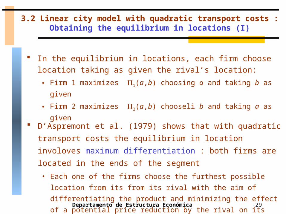
In the equilibrium in locations, each firm choose location taking as given the rival’s location:

• Firm 1 maximizes 1(a,b) choosing a and taking b as given

• Firm 2 maximizes 2(a,b) chooseli b and taking a as given

D’Aspremont et al. (1979) shows that with quadratic

transport costs the equilibrium in location involoves

maximum differentiation : both firms are located in the ends

of the segment

• Each one of the firms choose the furthest possible location from

its from its rival with the aim of differentiating the product and

minimizing the effect of a potential price reduction by the rival

on its own demand

3.2 Linear city model with quadratic transport costs :Obtaining the equilibrium in locations (I)


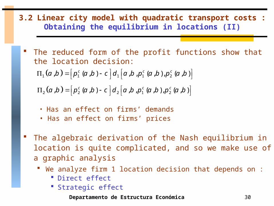
The reduced form of the profit functions show that the location decision:

1 1 1 1 2, ( , ) , , ( , ), ( , )c c ca b p a b c d a b p a b p a b

2 2 2 1 2, ( , ) , , ( , ), ( , )c c ca b p a b c d a b p a b p a b

• Has an effect on firms’ demands • Has an effect on firms’ prices

The algebraic derivation of the Nash equilibrium in location is quite complicated, and so we make use of a graphic analysis We analyze firm 1 location decision that depends on :

Direct effect Strategic effect

3.2 Linear city model with quadratic transport costs :Obtaining the equilibrium in locations (II)


Direct effect: for a given pair of prices ( ) and a given the location of firm 2, as firm 1 moves its location towards the location of firm 2 (i.e. towards the center of the segment) its demand increase, and so its profis.

1 2,p p

a’

d1’

d1

a

0 L1p 2p

L-b

Direct effect minimum differentiation tendency

xx’

3.2 Linear city model with quadratic transport costs :Obtaining the equilibrium in locations (III): direct effect


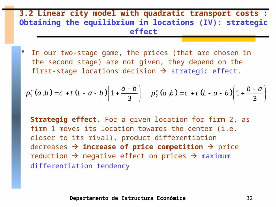
In our two-stage game, the prices (that are chosen in the second stage) are not given, they depend on the first-stage locations decision strategic effect.

Strategig effect. For a given location for firm 2, as firm 1 moves its location towards the center (i.e. closer to its rival), product differentiation decreases increase of price competition price reduction negative effect on prices maximum differentiation tendency

1 , 13

c a bp a b c t L a b

2 , 1

3c b a

p a b c t L a b

3.2 Linear city model with quadratic transport costs :Obtaining the equilibrium in locations (IV): strategic effect


d1

p2’

p1

a

p2

L-bxx’

L0

1d

1 'd

3.2 Linear city model with quadratic transport costs :Obtaining the equilibrium in locations (V): strategic effect


p2’

d1’

Strategic effect: maximum differentiation tendency

a’x’

x

p2

d1L0

a

p1

L-b

1 'd1d

3.2 Linear city model with quadratic transport costs :Obtaining the equilibrium in locations (VI): strategic effect


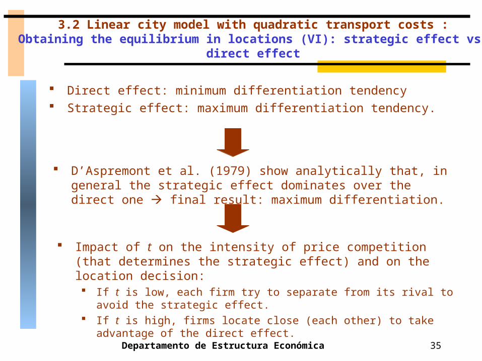
Direct effect: minimum differentiation tendency Strategic effect: maximum differentiation tendency.

D’Aspremont et al. (1979) show analytically that, in general the strategic effect dominates over the direct one final result: maximum differentiation.

Impact of t on the intensity of price competition (that determines the strategic effect) and on the location decision: If t is low, each firm try to separate from its rival to avoid the

strategic effect. If t is high, firms locate close (each other) to take advantage of

the direct effect.

3.2 Linear city model with quadratic transport costs :Obtaining the equilibrium in locations (VI): strategic effect vs. direct effect


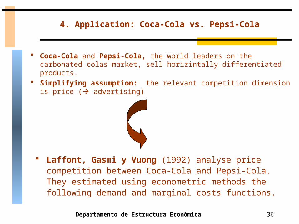
4. Application: Coca-Cola vs. Pepsi-Cola

Coca-Cola and Pepsi-Cola, the world leaders on the carbonated colas market, sell horizintally differentiated products.

Simplifying assumption: the relevant competition dimension is price ( advertising)

Laffont, Gasmi y Vuong (1992) analyse price competition between Coca-Cola and Pepsi-Cola. They estimated using econometric methods the following demand and marginal costs functions.


Demand functions for Coca-Cola (product 1) and Pepsi-Cola (product 2).

Q1 = 63.42 - 3.98 p1 + 2.25 p2

Q2 = 49.52 - 5.48 p2 + 1.40 p1

c1=4.96

c2=3.96

Marginal costs for Coca-Cola and Pepsi-Cola

Which is the optimal price for Coca-Cola and Pepsi-Cola?

4. Application: Coca-Cola vs. Pepsi-Cola: demand and costs functions


Step 1: solve the maximization problems of Coca-Cola and Pepsi-Cola.

• Coca-Cola’s maximization problem:

1

1 1 1 2( 4.96)(63.49 3.98 2.25 )p

Max p p p

*1 2 2( ) 10.44 0.28p p p Coca-Cola’s reaction function

• Pepsi-cola’s maximization problem:

2

2 2 2 1 ( - 3.96)(49.52- 5.48 1.40 )p

Max p p p

*2 1 1( ) 6.49 0.127p p p Pepsi-Cola’s reaction function

4. Application: Coca-Cola vs. Pepsi-Cola: optimal prices determination


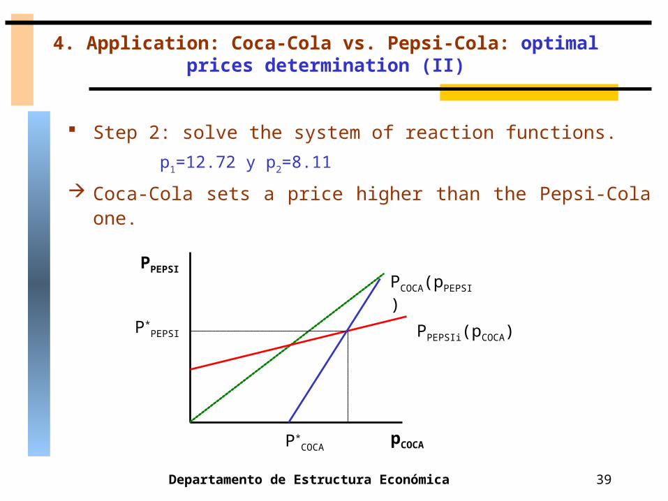
Step 2: solve the system of reaction functions.

p1=12.72 y p2=8.11

Coca-Cola sets a price higher than the Pepsi-Cola one.

4. Application: Coca-Cola vs. Pepsi-Cola: optimal prices determination (II)

PPEPSI

pCOCA

PCOCA(pPEPSI)

PPEPSIi(pCOCA)

P*COCA

P*PEPSI


Why Coca-Cola’s price is higher that Pepsi-Cola’s

one?

4. Application: Coca-Cola vs. Pepsi-Cola: optimal prices determination (III)

• Cost asymmetries

• Demand asymmetries


Costs asymmetries:

• Coca-Cola marginal cost (4.96) > Pepsis-Cola marginal cost (3.96)

Coca-Cola’s price > Pepsi-Cola’s price

4. Application: Coca-Cola vs. Pepsi-Cola: optimal prices determination (IV)


Demand asymmetries

Q1=63.42 - 3.98 p1+ 2.25

p2

Q2=49.52 - 5.48 p2+ 1.40

p1

p1= p2=p Q1=63.42 -1.73p

Q2=49.52 -4.08p

Graphic analysis normalize p=1 • Q1= 61.69 y Q2=45.44

• Q=Q1+Q2=107.13

4. Application: Coca-Cola vs. Pepsi-Cola: optimal prices determination (V)

2. Aymmetric Eq.a’>b Q1>Q2

Q1= 61.69 Q1= 45.44

1. Symmetric Eq. a=b Q1=Q2

Q1= 53.565 Q2= 53.565

a L-b

p=1 p=1

a’


The higher Coca-Cola’s price is due to:• Higher marginal cost (cost asymmetries)

• Demand asymmetries that favour Coca-Cola

4. Application: Coca-Cola vs. Pepsi-Cola: optimal prices determination (VI)


Do these asymmetries have any additional impact? price-cost margin

1 1

11

12.72 4.960.61

12.72p c

PCMp

2 2

22

8.11 3.960.51

3.96p c

PCMp

The price-cost margin of Coca-Cola is higher than the Pepsi-Cola’s one Demand asymmetry in favour of Coca-Cola Higher market power for Coca-Cola

4. Application: Coca-Cola vs. Pepsi-Cola: optimal prices determination (VII)


Product differentiation solves the Bertrand paradox:

• It allows firms to set price above marginal cost

• It allows firms to obtain positive profits

Firm will intend to differentiate their products (from those

of its competitors) as much as possible, the aim is to

reduce the intensity of price competition:

• Actual product differentiation

• Perceived product differentiation: increase consumers’

preference for the products of the firm

5. Concluding Remarks


Documents

Topic 6. Product differentiation (I): patterns of price setting Economía Industrial Aplicada Juan Antonio Máñez Castillejo Departamento de Estructura Económica