1

SACE Stage 2: Earth and Environmental Science

Topic 3: Climate Change

NASA (North American Space Agency) provide an excellent resource for climate change studies at

https://climate.nasa.gov/system/content_pages/main_images/1321_cc-vs-gw-vs-wx-768px.jpg

“Time is the school in which we learn,

Time is the fire in which we burn”

Delmore Schwartz (1913 – 1966)

Version 1 notes by Bernd Michaelsen

Monday_11_December_2017

2

Topic 3: Climate change

In this topic, students explore how climate variables have changed over geological time,

due to natural processes occurring in the Earth’s atmosphere, outside the atmosphere, and

within the Earth. They recognise why significant variation in Earth’s climate has the

potential to produce a major effect on Earth’s systems and on life on this planet.

Students analyse secondary data from geological, prehistorical, historical, and

contemporary records to interpret trends that provide evidence of past changes in climate.

They also explore the impact that human activities have had on recent changes in Earth’s

climate and how changes in oceanic circulation can affect weather systems.

Students use critical-thinking skills to consider different interpretations of the scientific

evidence for climate-change models, and the validity and reliability of these models in

predicting future climate change. They develop and extend their skills in communicating

scientific information by analysing and presenting evidence, and drawing and justifying

conclusions. They recognise how scientific knowledge from global collaboration can be

used to consider the future health and well-being of the global population

NOTE TO TEACHERS:

These notes have been designed to elaborate on the Possible Contexts provided in the

Earth and Environmental Science subject outline. They are intended to provide further

ideas and links to teaching and learning resources that address the Science Understanding.

It is important to remember that you are not expected to cover all of the material included.

Rather, these notes should be regarded as a ‘smorgasbord’ from which individual teachers

might pick and choose, according to the needs and abilities of their students and according

to the context of their externally assessed ‘Earth Systems Study’.

3

Science Understanding Possible Contexts

Natural processes in the Earth’s atmosphere affect climate change over geological time.

Discuss the evolution of the Earth’s atmosphere.

Explain how the composition of the Earth’s atmosphere changes over time.

Discuss the greenhouse effect.

Explain how the lifespans of greenhouse gases and their ability to absorb infrared radiation contribute to their warming potentials.

Discuss how solar energy is absorbed, re-emitted, and reflected by atmospheric gases and the Earth’s surface, including the albedo effect.

Watch the SciShow YouTube video, ‘A History of Earth’s Climate’ (includes natural and anthropogenic factors).

https://youtu.be/dC_2WXyORGA

Watch and discuss Australia: The Time Traveller’s Guide about the evolution of the Australian continent.

www.abc.net.au/tv/programs/australia-the-time-travellers-guide/

Investigate how the composition of the atmosphere has changed over time, including greenhouse gases, water vapour, carbon dioxide, ozone, methane, and nitrous oxide, using:

Earthlearningidea, ‘Earth’s Atmosphere – A Step by Step Evolution’:

www.earthlearningidea.com/PDF/103_Evolution_atmosphere.pdf

PhET ‘The Greenhouse Effect’:

https://phet.colorado.edu/en/simulation/greenhouse

Earth System Science Education Alliance, ‘Water Vapour: Feedback or Forcing?’:

http://esseacourses.strategies.org/module.php?module_id=172

Explore the Earth’s energy budget with EarthLabs:

http://serc.carleton.edu/eslabs/weather/2b.html

Investigate the Earth’s energy budget through the EarthLabs activity:

http://d32ogoqmya1dw8.cloudfront.net/files/eslabs/weather/energy_balance_instructions.pdf

Natural processes outside of the Earth’s atmosphere affect climate change over geological time.

Explain how astronomical cycles affect natural climate variability.

Explain how variations in solar energy due to sunspot activity can contribute to natural climate change.

Investigate how the Milankovitch cycles and solar cycles affect natural climate variability.

4

Science Understanding Possible Contexts

Natural processes within the Earth affect climate change over geological time.

Explain how the plate-tectonic supercycle has contributed to global climatic changes throughout the Earth’s history.

Investigate how plate tectonics has influenced climate change over geological time.

Oceans absorb large amounts of solar radiation.

Explain the effect of water’s large specific heat capacity on changes in ocean temperature.

Investigate the specific heat capacity of various substances including water.

Changes in oceanic circulation may impact on weather systems.

Explain the difference between surface and deep-water ocean currents.

Explain the relationship between the world’s wind belts and the world’s surface ocean currents.

Explain the relationship between the thermohaline circulation and deep-water ocean currents.

Examine how continental distribution influences ocean currents.

Discuss the impact of mountain-building on elevation and hence climatic conditions.

Watch and discuss Australia: The Time Traveller’s Guide about the evolution of the Australian continent.

www.abc.net.au/tv/programs/australia-the-time-travellers-guide/

Investigate ocean currents and how they influence climate.

http://oceanservice.noaa.gov/education/tutorial_currents/welcome.html

Anthropogenic activities affect climate conditions.

Explain the enhanced greenhouse effect.

Describe anthropogenic activities that are changing the levels of greenhouse gases.

Compare how local, national, and global policies can affect the levels of these gases.

Explain how carbon is stored in Earth’s systems over a variety of time-scales.

Explore the global-warming potential (GWP) of carbon dioxide, methane, nitrous oxide, and hydrofluorocarbons.

Explore how land clearing and fossil fuel consumption can increase levels of greenhouse gases.

Examine the storage of carbon in the carbonate–silicate geochemical cycle.

Investigate state, territory, and/or national government policies related to climate change.

http://dfat.gov.au/international-relations/themes/climate-change/pages/climate-change.aspx

5

Science Understanding Possible Contexts

Examine evidence of past glaciations, interglacial periods, and atmospheric parameters to find a period in Earth’s history that can be used as an analogue for a future with an enhanced greenhouse effect.

Watch and discuss a TED talk, such as ‘Climate Change is Happening. Here’s How We Adapt’:

www.ted.com/talks/alice_bows_larkin_we_re_too_late_to_prevent_climate_change_here_s_how_we_adapt/transcript?language=en

Explore how global policies concerning chlorofluorocarbon (CFC) use brought a change to the levels of these gases in the atmosphere through the No Zone of Ozone activity.

Examine how to evaluate scientific claims:

http://www.exploratorium.edu/evidence/evidence.html?#/tester/

Climate change affects Earth systems.

Discuss the effects of climate change on Earth systems.

Investigate clathrate deposits on the ocean floor.

https://en.wikipedia.org/wiki/Methane_clathrate

Discuss whether the melting of sea ice will raise sea levels in the same way as the melting of continental ice sheets.

Explore the impacts of climate change on:

the biosphere, e.g. species distribution and crop productivity

atmosphere, e.g. rainfall patterns and surface air temperatures

hydrosphere, e.g. sea levels, ocean acidification, extent of ice sheets.

Explain how climate analogues can be used to explore the impact of climate change.

Explore the interactions between the spheres that occur during the melting of permafrost.

Discuss effects of climate change on natural carbon sequestration in the carbon cycle.

6

Explore the potential risks and benefits of using geosequestration to reduce atmospheric levels of carbon dioxide:

http://australianmuseum.net.au/blogpost/lifelong-learning/geosequestration-sweeping-co2-under-the-rug

Geological, prehistorical, historical, and contemporary records provide evidence that climate change has affected different regions and species differently over time.

Investigate how contemporary levels of CO2 and temperature are monitored, and provide evidence of contemporary climate change.

Explore how climate proxies are used to provide evidence of climate change.

Explore NOAA, ‘Paleo Proxy Data – What Is It?’:

www.ncdc.noaa.gov/paleo/primer_proxy.html

http://serc.carleton.edu/microbelife/topics/proxies/paleoclimate.html

Explore the evidence for the Medieval Warm Period.

Explore how historical and archaeological records, such as cave paintings, can be used to determine past climates.

Investigate climate change using foraminifera.

www.ucmp.berkeley.edu/fosrec/Olson2.html

Investigate the evidence for ‘The Little Ice Age: Understanding Climate and Climate Change’ using this CLEAN activity:

http://cleanet.org/resources/41810.html

Investigate how evidence from proxy data, such as isotopic ratios, ice-core data, palaeobotany, and the fossil record, has contributed to the development of models of climate change:

http://serc.carleton.edu/eslabs/climatedetectives/index.html

https://www.bas.ac.uk/data/our-data/publication/ice-cores-and-climate-change/

7

Models for predicting climate change are based on past climate data and are continually changing.

Explain how general circulation models can be used to predict future climate change.

Explore how global climate models are used to predict future climate, through watching and discussing ‘Modeling Our Climate’, Brown University:

https://www.youtube.com/watch?v=SuZHnqxltKo

Explain how the El Niño/La Niña events in the ocean–atmosphere system of the tropical Pacific Ocean can be predicted using climate models. Bureau of Meteorology, ‘What is El Nino and What Might It Mean for Australia?’:

www.bom.gov.au/climate/updates/articles/a008-el-nino-and-australia.shtml

Evaluate the usefulness of general circulation models:

www.ipcc-data.org/guidelines/pages/ gcm_guide.html

Investigate NASA global climate modelling:

www.giss.nasa.gov/projects/gcm/

Discuss the effectiveness of international collaboration of scientists at the Intergovernmental Panel on Climate Change (IPCC) in determining achievable targets for the reduction of global warming.

8

Natural processes in the Earth’s atmosphere affect climate change over geological time.

A brief (11 minute 19 second) history of climate change

The 11 minute 19 second video “A history of Earth’s climate” is packed with

great information and is an excellent summary of climate change: https://www.youtube.com/watch?v=dC_2WXyORGA

Amongst other things, in this topic (Climate Change) we shall explore in more

detail what has been asserted in the video.

Earth’s atmosphere – some terminology

Troposphere

The troposphere, the lowest atmospheric layer extends to between ~8 and ~ 15

km, the approximate altitude that conventional jet aircraft fly.

Nearly all weather variations occur in the troposphere

(https://scied.ucar.edu/atmosphere-layers). Ninety-nine (99.13%) of the atmosphere’s

water vapour is within the troposphere.

Schematic summary of Earth’s inner and middle atmosphere to an altitude of 100 km.

Stratosphere

The stratosphere extends from the upper boundary of the troposphere, to ~ 50

km above Earth’s surface. The stratosphere includes the so-called ozone layer

(~20–30 km above Earth’s surface) where molecules of ozone (O3) absorb high-

energy ultra-violet (UV) and other electromagnetic radiation from the Sun and

outer-space.

9

Molecular structure of ozone (O3). Note that there is a convention regarding the colours used to represent atoms in molecular models (https://en.wikipedia.org/wiki/CPK_coloring)

Commercial jet aircraft purposefully fly in the lower stratosphere because the

stratosphere is less turbulent than the underlying troposphere. Counter-

intuitively, temperatures in the stratosphere increase with height (see above

figure).

Mesosphere

The mesosphere extends beyond the stratosphere to an altitude of ~85 km.

Unlike the underlying stratosphere, temperature within the mesosphere

systematically decreases with height. Most meteors that enter Earth’s

atmosphere burn-up in the mesosphere (https://scied.ucar.edu/atmosphere-layers).

Thermosphere

Above the mesosphere is the thermosphere, a layer which absorbs large

amounts of high-energy X-rays and UV radiation; consequently, its

temperature is typically in the range between 200 and 500 °C. The upper

boundary of the thermosphere varies between ~500 and 1000 km from Earth’s

surface due to changes in radiation from the Sun.

In the upper thermosphere, X-rays and UV radiation are responsible for

breaking apart molecules and consequently atom oxygen (O), atomic nitrogen

(N) and atomic helium (He) are its main components.

Exosphere

The exosphere (sometimes considered a part of the thermosphere) exists

beyond the thermosphere, and is in effect an ultra-diluted atmosphere

extending to ~10,000 km, representing molecules that have escaped Earth’s

gravitational pull. However, for practical purposes, the exosphere must be

considered as part of outer space.

Ionosphere

The term ionosphere encompasses a number of regions within the upper

mesosphere to the thermosphere (see figure below).

10

D, E, and F layers of Earth’s ionosphere within the mesosphere and the thermosphere, by Randy Russell, UCAR Centre for Science Education (https://scied.ucar.edu/ionosphere)

Regions of the ionosphere are not considered separate layers but are regions

coinciding with formation of ionized particles within the standard atmospheric

layers.

“The ionosphere is a critical link in the chain of Sun-Earth interactions” (https://www.nasa.gov/mission_pages/sunearth/science/atmosphere-layers2.html)

The rate of formation of ions in the ionosphere is seasonally influenced and

varies with latitude. The 11-year sunspot cycle and solar flares and coronal

mass injections greatly influences the ionosphere and can have a temporarily

effect of disrupting satellite and GPS navigation and information systems.

Discuss the evolution of the Earth’s atmosphere.

There is abundant evidence in the geological record of an ever-changing Earth climate.

Presently, N2 makes-up ~78% of Earth’s total atmosphere, with lesser

amounts of O2 (~21%), Ar (~0.9%) and CO2 (~0.4%), as well as others.

However, Earth’s atmosphere and climate have been ever-changing since

Earth’s formation at ~ 4.56 Ga.

Initially Earth was molten; its dense core (Topic 1: Earth Systems) formed

very early in earth’s history soon at ~ 4.52 Ga.

For the first ~2 billion years of its existence, Earth’s hydrosphere evolved as

H2O was added by volcanic activity and the proportion of CO2 also increased.

The composition of Earth’s atmosphere also changed as volcanism brought

other gases to the surface – these included He, CH4, ammonia (NH3), H2S,

CO2, SO2, H2S, and the relatively inert N2.

11

During the early Hadean, light elements such as He and H2 were lost because

they escaped Earth’s gravitational field (it is likely that Earth’s

magnetosphere was not as strong as it is now and therefore did not protect

Earth’s atmosphere in the way it does now, for example).

Composition of Earth’s atmosphere, from its formation (4.6 Ga) to the present (http://www.scientificpsychic.com/etc/timeline/atmosphere-composition.html)

“Faint Young Sun paradox”: During the Hadean, the Sun only emitted ~30%

of the radiation that it presently does. With such a low emission of radiation,

one would expect a “frozen” Earth’s surface. Yet there is evidence of liquid

water on Earth (see below). The best explanation for this paradox is that

Earth’s atmosphere must have contained very high levels of greenhouse gases,

such as methane and ammonia.

As Earth’s surface cooled, H2O was removed from the atmosphere as

water vapour condensed to form the oceans.

First evidence of liquid water at Earth’s surface is at ~ 4.4 Ga. The fact

of liquid water constrains the temperature at Earth surface at this time

to < 100 °C

Due to on-going volcanism, atmospheric CO2 increased until about the

mid-Archean, then depleted as carbonate minerals formed as a result of

reactions between metals and carbonic acid (i.e. CO2 dissolved in water).

12

Atmospheric oxygen

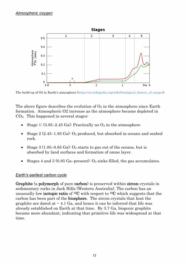
The build-up of O2 in Earth’s atmosphere (https://en.wikipedia.org/wiki/Geological_history_of_oxygen)

The above figure describes the evolution of O2 in the atmosphere since Earth

formation. Atmospheric O2 increase as the atmosphere became depleted in

CO2. This happened in several stages:

Stage 1: (3.85–2.45 Ga): Practically no O2 in the atmosphere

Stage 2 (2.45–1.85 Ga): O2 produced, but absorbed in oceans and seabed

rock.

Stage 3 (1.85–0.85 Ga): O2 starts to gas out of the oceans, but is

absorbed by land surfaces and formation of ozone layer.

Stages 4 and 5 (0.85 Ga–present): O2 sinks filled, the gas accumulates.

Earth’s earliest carbon cycle

Graphite (a polymorph of pure carbon) is preserved within zircon crystals in

sedimentary rocks in Jack Hills (Western Australia). The carbon has an

unusually low isotopic ratio of 13C with respect to 12C which suggests that the

carbon has been part of the biosphere. The zircon crystals that host the

graphite are dated at ~ 4.1 Ga, and hence it can be inferred that life was

already established on Earth at that time. By 3.7 Ga, biogenic graphite

became more abundant, indicating that primitive life was widespread at that

time.

13

Timeline of life and evolution of Earth’s atmosphere (https://en.wikipedia.org/wiki/Late_Heavy_Bombardment)

Build-up of N2 in the atmosphere

Nitrogen gas (N2) was probably always present in Earth’s atmosphere.

However, because N2 it is relatively inert it’s concentrations increased

significantly from the early Archean onwards. Today it is the most abundant

atmospheric gas comprising ~78% of Earth atmosphere.

14

Explain how the composition of the Earth’s atmosphere changes over time

Schematic of volcanic eruption highlighting flux of volcanic gasses and their reactions in the upper atmosphere, by the United States Geological Survey (https://en.wikipedia.org/wiki/Volcanic_gas)

For the first 0.7 billion years or so of its history (i.e. 4.56 – 3.8 Ga), Earth was

bombarded by meteorites and asteroids (bolides), and would have been very

inhospitable. The frequency of meteorite bombardment peaked during what is

geologists call the Late Heavy Bombardment (LHB), between ~4.1 and 3.8 Ga.

A high frequency of meteorite bombardment would have brought with it water

but much of the volcanic gases and water that made-up the atmosphere would

have been ejected into space and lost to Earth’s gravitational pull.

What’s the difference between a meteorite and an asteroid?

By-the-way: It is postulated that much, if not most of the heavy elements such

as Au, Ag, Pt, Ni, Co, Fe, U etc. that are presently part of Earth’s lithosphere

were sourced from the LHB. The heavy elements that were present when the

Earth-Moon system formed had sunk towards Earth’s centre due to gravity,

and have been part of Earth’s core since its formation (4.52 Ga).

Stromatolites in Shark Bay, Western Australia. Scale: Individual stromatolites are ~ 30 cm above sand. Shark Bay is one of the few places in the world where stromatolites still exist. Photo: https://www.skyscanner.com.au/news/unusual-and-awesome-things-to-do-in-western-australia

15

The so-called “Great Oxidation Event” at ~ 2.5 Ga, coinciding with the end of

the Archean, is arguably the most important change in Earth’s atmosphere.

At around this time, stromatolites (see figure above) comprising layers of

photosynthesizing cyanobacteria (present on Earth since ~3.7 Ga) began to

produce more plentiful atmospheric O2.

The removal of large quantities of CO2 from the atmosphere was probably the

trigger the Earth’s first major glaciation, the Huronian glaciation at ~2.4 to 2.1 Ga.

Based on many substantiated lines of evidence, published in peer-reviewed

scientific journals, it is clear that life on Earth evolved around 4.1–3.8 Ga, and

possibly slightly earlier than 4.1 Ga, i.e. around the commencement of the

LHB.

Initially life comprised only single celled prokaryotes (cyanobacteria,

archaebacterial, purple bacteria). It is unclear when eukaryotes evolved;

however, most evolutionally biologists agree that eukaryotic life had evolved

by at least ~2.2 Ga if not earlier; almost certainly after the Great Oxidation

Event.

The first segmented and complex animals, the Ediacaran fauna evolved

around ~635 Ma, at the start of the Ediacaran Period. At this time there was

a further increase in atmospheric O2, and a concomitant warming of the

atmosphere.

The Ediacaran fauna are named after the Ediacaran Hills, a relatively low-

lying range of hills west of the Flinders Ranges, South Australia.

What kind of animals are represented by the Ediacaran fossils?

16

Discuss the greenhouse effect

The greenhouse effect is a process which warms Earth’s atmosphere due to the

absorption of radiation energy by several gases; these greenhouse gases allow

solar radiation to reach Earth’s surface but then absorbs the energy as it is

reemitted as infrared radiation, acting to contain the heat within the

atmosphere; this occurs naturally and is increased by humans (see enhanced

greenhouse effect).

Schematic diagram showing global energy flow through Earth’s atmosphere, by Kevin Trenberth, John Fasullo and Jeff Kiefl of UCAR, Centre for Science Education (https://scied.ucar.edu/radiation-budget-diagram-earth-atmosphere)

The above figure illustrates the flow of energy through Earth’s atmosphere.

The vectors for solar radiation are shown in dark yellow; vectors for outgoing

longwave radiation are shown in buff colour. The energy differential between

the incoming and outgoing radiation causes the greenhouse effect.

According to the United States’ National Oceanic and Atmospheric

Administration (NOAA), the composition of Earth’s present (2009) atmosphere

is:

N2 (78.1%), molecular nitrogen,

O2 (20.9%), molecular oxygen,

Ar (0.9%), argon,

CO2 (0.039%), carbon dioxide,

CH4 (0.000,18%), methane,

N2O (0.000,032%), nitrous oxide, and

SF6 (0.000,000,000,67%), sulphur hexafluoride.

Influential greenhouse gases highlighted in red.

The important point is that the major non-greenhouse gases, N2, O2 and Ar in

combination, account for 99.5% of the entire atmosphere, but they have little if

any effect on global temperatures because they do not absorb visible or

infrared radiation (https://www.esrl.noaa.gov/gmd/outreach/carbon_toolkit/basics.html).

17

NOAA’s Earth System Research Laboratory has web-published an excellent

summary of the greenhouse effect and the major greenhouse gases. The text

below is largely reproduced from

https://www.esrl.noaa.gov/gmd/outreach/carbon_toolkit/basics.html.

Carbon dioxide

Carbon dioxide (CO2) is a colorless, odorless gas consisting of molecules made

up of two oxygen atoms and one carbon atom. Carbon dioxide is produced

when an organic carbon compounds (such as lignin and cellulose in wood) or

fossilized organic matter (such as coal, oil, or natural gas) is burned in the

presence of oxygen. Carbon dioxide is removed from the atmosphere by carbon

dioxide "sinks", such as absorption by seawater and photosynthesis by ocean-

dwelling plankton and land plants, including forests and grasslands.

However, seawater is also a source of CO2 to the atmosphere, along with land

plants, animals, and soils, when CO2 is released during respiration.

Methane

Methane (CH4) is a colorless, odorless non-toxic gas consisting of molecules

made up of four hydrogen atoms and one carbon atom. Methane is

combustible, and it is the main constituent of natural gas, a fossil fuel.

Methane is released when organic matter decomposes in low oxygen

environments. Natural sources include wetlands, swamps and marshes,

termites, and oceans. Human sources include the mining of fossil fuels and

transportation of natural gas, digestive processes in ruminant animals such as

cattle, rice paddies and the buried waste in landfills. Most methane is

eventually broken down in the atmosphere by reacting with small very

reactive molecules called hydroxyl (OH) radicals.

Nitrous oxide

Nitrous oxide (N2O) is a colorless, non-flammable gas with a sweetish odor,

commonly known as "laughing gas", and sometimes used as an anesthetic.

Nitrous oxide is naturally produced in the oceans and in rainforests. Man-

made sources of nitrous oxide include the use of fertilizers in agriculture,

nylon and nitric acid production, cars with catalytic converters and the

burning of organic matter. Nitrous oxide is broken down in the atmosphere by

chemical reactions driven by sunlight.

Sulfur hexafluoride

18

Sulfur hexafluoride (SF6) is an extremely potent greenhouse gas. SF6 is very

persistent, with an atmospheric lifetime of more than a thousand years. Thus,

a relatively small amount of SF6 can have a significant long-term impact on

global climate change. SF6 is human-made, and the primary user of SF6 is the

electric power industry. Because of its inertness and dielectric properties, it is

the industry's preferred gas for electrical insulation, current interruption, and

arc quenching (to prevent fires) in the transmission and distribution of

electricity. SF6 is used extensively in high voltage circuit breakers and

switchgear, and in the magnesium metal casting industry.

Water

Is water vapour a greenhouse gas? To begin to answer this question, start your research at http://esseacourses.strategies.org/module.php?module_id=172

Interactively explore the “Greenhouse Effect” at https://phet.colorado.edu/en/simulation/greenhouse

This interactive simulation allows you to compare the incoming “sunlight”

photons” with outgoing infrared” photons under different greenhouse gas

compositions.

Ozone

Ozone is a greenhouse gas, with over 90% being concentrated in the

stratosphere.

19

Explain how the lifespans of greenhouse gases and their ability to absorb infrared radiation contribute to their warming potentials

Gases in the atmosphere have different lifetimes, and the greater the lifetime,

the greater their warming potential.

The Intergovernmental Panel on climate Change (IPCC) publish a very

comprehensive list of greenhouse gases

(http://www.ipcc.ch/publications_and_data/ar4/wg1/en/ch2s2-10-2.html#table-2-14).

Many of the data refer to anthropogenic CFCs and hydrofluorocarbons

(HCFCs) that are, thankfully in very low abundance in the lower atmosphere.

In summary, the main effective greenhouse gases are (with atmospheric

concentration and greenhouse contribution in %):

H2O vapour and clouds (10–50,000 ppm; 36–72%)

CO2 (~400 ppm; 9–26%)

CH4 (~1.8 ppm; 4–9%)

Ozone (2–8 ppm; 3–7%)

Source: https://en.wikipedia.org/wiki/Greenhouse_gas#Greenhouse_gases

How long do greenhouse gases stay in the atmosphere?

The persistence of various greenhouse gases in Earth’s atmosphere is very

complex science, to say the least. However, it is possible to make some

generalisations:

CO2: Several processes remove CO2 from the atmosphere – between 65% and

80% of CO2 released into the atmosphere is eventually (presently) dissolved

into the oceans over a 20–200 year period

(https://www.theguardian.com/environment/2012/jan/16/greenhouse-gases-remain-air). The

remainder is removed by processes such as deposition of carbonate rock, for

example.

Methane: Methane lasts approximately 12 years in the atmosphere before it is

oxidised to CO2 and H2O.

Nitrous oxide (N2O): Nitrous oxide persists for about 114 years before

breaking-down, i.e. its lifetime is one order of magnitude greater than that of

methane.

What is the lifetime of water vapour in the atmosphere?

Radiative efficiencies of some greenhouse gases

The radiative efficiency (W.m-2.ppb-1) is the capacity of a gas to absorb infrared

radiation and therefore contribute to global warming. Data published by the

IPCC indicate the following radiative efficiencies for the main anthropogenic

greenhouse gases:

20

CO2 (1.4x10-5)

CH4 (3.7x10-4)

N2O (3.03x10-3)

Notice the different orders of magnitude for these gases.

Global warming potential

A consequence of these data is that over a 100-year time-span, one molecule of

methane has 25 times the greenhouse warming potential as does one molecule

of CO2. And one molecule of nitrous oxide has ~300 times the greenhouse

warming potential than does one molecule of CO2.

Study the technical data from the IPCC at https://www.ipcc.ch/publications_and_data/ar4/wg1/en/ch2s2-10-2.html With respect to CO2, what is the global warming potential of CFCs and hydrofluorocarbons?

What is the Montreal protocol?

2014 atmospheric nitrogen dioxide (NO2) levels (https://en.wikipedia.org/wiki/Greenhouse_gas#Greenhouse_gases)

Nitrogen dioxide (NO2) is different to nitrous oxide (N2O). What are the anthropogenic sources of both?

Discuss how solar energy is absorbed, re-emitted, and reflected by atmospheric gases and Earth’s surface, including the albedo effect

21

For more on the Earth-atmosphere energy balance visit http://www.srh.noaa.gov/jetstream/atmos/energy.html

Earth’s solar energy budget courtesy of the (USA) National Science Digital Library (http://esseacourses.strategies.org/module.php?module_id=99)

The entire Earth system has an energy budget – energy is derived either from

space (i.e. mostly from the Sun), or energy derived from radiogenic processes

within Earth; however, in this discussion, we exclude any consideration of

energy derived radioactive decay within the geosphere.

Earth’s energy budget might be described as all gains of radiation energy from

beyond the atmosphere (incoming) and all outgoing energy. If the flow of

incoming energy would be the same as the amount of outgoing (reflected)

energy, Earth would be in a state of radiative equilibrium.

If Earth were not in a state of radiative equilibrium, global temperatures

would rise or fall accordingly.

Albedo effect

The word albedo is Latin meaning “whiteness”. Within a modern scientific

context, it is used to describe a measure of “brightness”.

Albedo is measured on a scale of 0 to 1 (alternatively 0 – 100%):

Objects or material scoring 0 are black and reflect no light.

Objects or material scoring 1 (100%) are white and reflect all incident

light.

22

Schematic representation of albedo effect (http://climate.ncsu.edu/edu/k12/.albedo)

The albedo effect, i.e. the amount of radiation reflected from different

materials at or near Earth’s surface. The albedo effect is therefore

fundamentally important to considerations of the weather and climate.

A common scenario that illustrates the albedo effect is that of walking on the

beach on a hot (> 35 °C) summer’s day: Walking on dark coloured sand is

unbearably hot and almost immediately burns the soles of the feet; whereas

walking on highly-reflective white sand can be endured for a long time before

burning occurs.

Fresh snow and liquid water has albedo values of 0.95 and 0.10 respectively

0.10.

How do these values compare with the albedo data in the figure below? Why are there differences?

Albedo: % of diffusely reflected sunlight in relation to various surface conditions (https://en.wikipedia.org/wiki/Albedo)

Since ~30% of the Sun’s radiation is reflected by Earth as a whole, it’s correct

to say that Earth’s albedo is 0.3.

23

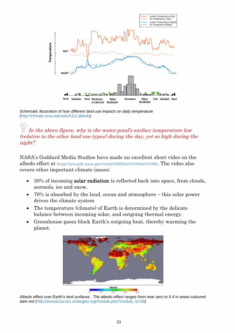
Schematic illustration of how different land use impacts on daily temperature (http://climate.ncsu.edu/edu/k12/.albedo)

In the above figure, why is the water pond’s surface temperature low (relative to the other land-use types) during the day, yet so high during the night?

NASA’s Goddard Media Studios have made an excellent short video on the

albedo effect at https://svs.gsfc.nasa.gov/vis/a010000/a010100/a010198/. The video also

covers other important climate issues:

30% of incoming solar radiation is reflected back into space, from clouds,

aerosols, ice and snow.

70% is absorbed by the land, ocean and atmosphere – this solar power

drives the climate system

The temperature (climate) of Earth is determined by the delicate

balance between incoming solar, and outgoing thermal energy.

Greenhouse gases block Earth’s outgoing heat, thereby warming the

planet.

Albedo effect over Earth’s land surfaces. The albedo effect ranges from near zero to 0.4 in areas coloured dark red (http://esseacourses.strategies.org/module.php?module_id=99)

24

Mean annual albedo, 2003 – 2004: Upper image: clear sky. Lower image: total sky (https://en.wikipedia.org/wiki/Albedo)

Compare and contrast the reflectivity data of the images for Earth’s clear sky

albedo and its total sky albedo. Areas of Earth with the highest average mean

annual albedo are Antarctica and Greenland that are covered in ice and snow

(frozen H2O). By contrast, areas of the globe with the lowest albedo are the

oceans (liquid H2O).

Do you think this SACE course (i.e. Earth & Environmental Science), would be offered in the school curriculum if liquid water had an albedo effect similar to that of fresh snow? Explain your answer.

As we have seen Earth only reflects about 30% of all radiation that it receives

from the Sun. In the short-term, the consequences of this will be a global rise

in temperatures that will cause:

a continued melting of the polar ice caps

less snow on mountain ranges

melting of mountain glaciers in the Himalayas, the European Alps, the

Americas and elsewhere.

In recorded history, only two mountains in Africa have had glaciers. Which are these and what has become of their glaciers in the last 30 years?

25

With increased melting of glaciers and the heating of the oceans there will be

increased water vapour in the atmosphere. Additional clouds may of course

increase Earth’s overall albedo – maybe.

For a good discussion on the reflectivity of clouds and albedo, visit

http://esseacourses.strategies.org/module.php?module_id=99.

Natural processes outside of Earth’s atmosphere affect climate change over geological time.

Explain how astronomical cycles affect natural climate variability

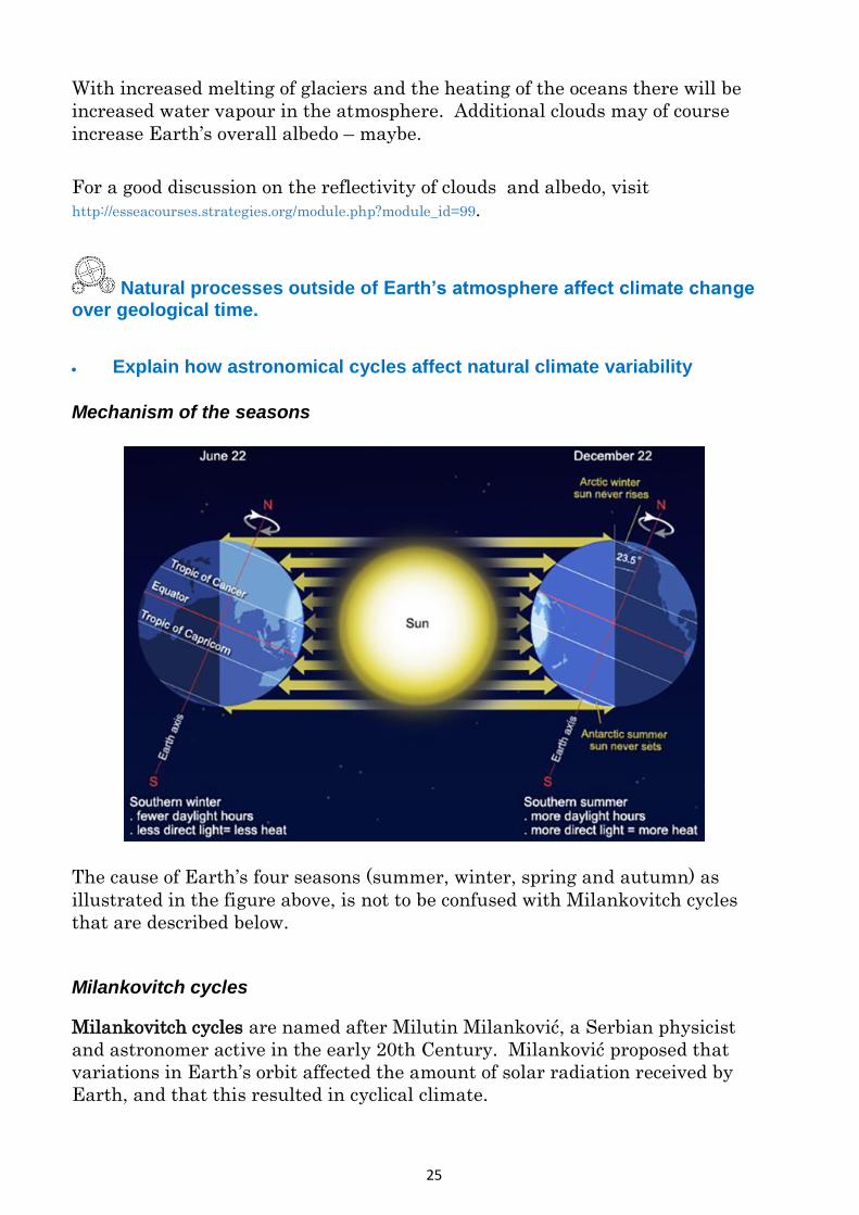
Mechanism of the seasons

The cause of Earth’s four seasons (summer, winter, spring and autumn) as

illustrated in the figure above, is not to be confused with Milankovitch cycles

that are described below.

Milankovitch cycles

Milankovitch cycles are named after Milutin Milanković, a Serbian physicist

and astronomer active in the early 20th Century. Milanković proposed that

variations in Earth’s orbit affected the amount of solar radiation received by

Earth, and that this resulted in cyclical climate.

26

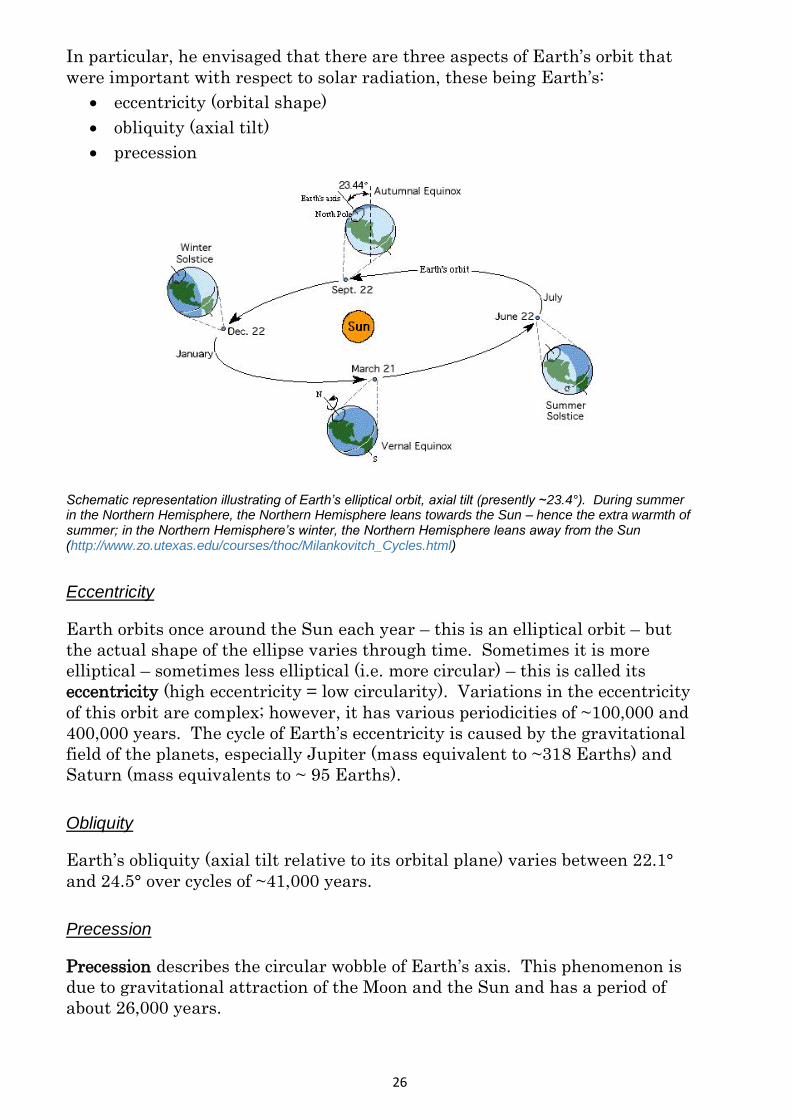
In particular, he envisaged that there are three aspects of Earth’s orbit that

were important with respect to solar radiation, these being Earth’s:

eccentricity (orbital shape)

obliquity (axial tilt)

precession

Schematic representation illustrating of Earth’s elliptical orbit, axial tilt (presently ~23.4°). During summer in the Northern Hemisphere, the Northern Hemisphere leans towards the Sun – hence the extra warmth of summer; in the Northern Hemisphere’s winter, the Northern Hemisphere leans away from the Sun (http://www.zo.utexas.edu/courses/thoc/Milankovitch_Cycles.html)

Eccentricity

Earth orbits once around the Sun each year – this is an elliptical orbit – but

the actual shape of the ellipse varies through time. Sometimes it is more

elliptical – sometimes less elliptical (i.e. more circular) – this is called its

eccentricity (high eccentricity = low circularity). Variations in the eccentricity

of this orbit are complex; however, it has various periodicities of ~100,000 and

400,000 years. The cycle of Earth’s eccentricity is caused by the gravitational

field of the planets, especially Jupiter (mass equivalent to ~318 Earths) and

Saturn (mass equivalents to ~ 95 Earths).

Obliquity

Earth’s obliquity (axial tilt relative to its orbital plane) varies between 22.1°

and 24.5° over cycles of ~41,000 years.

Precession

Precession describes the circular wobble of Earth’s axis. This phenomenon is

due to gravitational attraction of the Moon and the Sun and has a period of

about 26,000 years.

27

Schematic showing difference in between eccentricity, precession and obliquity (https://www.universetoday.com/39012/milankovitch-cycle/)

The combination of changes in Earth’s eccentricity, axial tilt and precession

results in climatic cycles of about 21,000, 41,000, 100,000 and 400,00 years.

Recession of the Moon

The recession of the Moon is not to be confused with the precession of Earth’s

axis of rotation.

Recession of the Moon describes the movement of the Moon away from Earth.

Presently the Moon revolves around Earth following an elliptical orbit, similar

to the orbit of Earth around the Sun, and the Moon’s gravitational pull causes

tidal action on Earth.

Despite its elliptical orbit which is on average ~384,400 km around Earth’s

centre, the movement of the Moon away from Earth can be measured quite

accurately at 3.82 ± 0.07 centimetres per annum. This is due to the fact that

earth rotates faster on its own axis than the Moon revolves around Earth.

For more information on this matter visit

https://rationalwiki.org/wiki/Recession_of_the_Moon

The Moon’s elliptical r revolution around Earth stabilises Earth’s own rotation about its axis. But what will happen when the Moon eventually moves into an orbit so distant from Earth that it’s gravitational pull is inadequate to produce oceanic tides on Earth? And what will be the consequences to Earth’s ecosystem?

Explain how variations in solar energy due to sunspot activity can contribute to natural climate change

Solar cycle

28

The solar cycle (aka solar magnetic activity cycle) is an 11-year cycle in the

change of solar radiation and other phenomena, predominantly sunspots, but

also coronal loops and coronal mass injections.

The solar maximum is that part of the solar cycle where the sunspot activity is

at a maximum.

At temperatures of only 3000 – 4500 K, sunspots are cooler than the Sun’s

immediately surrounding plasma at 5800 K.

To gain an appreciation of the scale of sunspots, watch some videos at

https://en.wikipedia.org/wiki/Sunspot.

Summary of 400 years of monitoring sunspot numbers. There are clearly 1st, 2nd and even 3rd order cycles (https://en.wikipedia.org/wiki/Sunspot)

Since 1979, satellites have measured sunspot numbers and solar radiation

received by Earth. Measurements taken show the energy received from the

sun changes about 0.1% on each cycle (i.e. 0.1% less energy is received from

the Sun during periods of high sunspot activity.

One conclusion to be drawn from this is that the recent increase in global

warming have not been caused by changes in solar radiation.

29

Figure is taken from https://www.skepticalscience.com/solar-activity-sunspots-global-warming.htm Annual global temperature change (thin light red) with 11 year moving average of temperature (thick dark red). Temperature from NASA GISS. Annual Total Solar Irradiance (thin light blue) with 11 year moving average of TSI (thick dark blue). TSI from 1880 to 1978 from Krivova et al 2007. TSI from 1979 to 2015 from the World Radiation Center (see their PMOD index page for data updates). Plots of the most recent solar irradiance can be found at the Laboratory for Atmospheric and Space Physics LISIRD site.

30

Natural processes outside of the Earth’s atmosphere affect climate change over geological time

Plate tectonic theory is a paradigm that attempts to explain Earth’s geological

dynamic processes – mountain building, movement of landmasses, volcanic

activity and earthquakes.

The movement of Earth’s tectonic plates is measured in centimetres per year;

for example, the Australian plate is presently moving about 7 cm NE per year.

Therefore, any climate change due to plate tectonics must logically be very

slow.

Plate tectonic motion based on GPS satellite data from NASA. Vectors show the direction and magnitude of motion (https://en.wikipedia.org/wiki/Plate_tectonics)

However, movement of continental land masses through geological time

causes changes to ocean currents and that in turn means major changes to

Earth’s climate. Changes to the position of continents, as well as island arcs

and mountain belts will cause changes to both atmospheric and oceanic

circulation.

Richard Sedlock (San José State University) has produced a superb video on

the effects of plate tectonics on Earth’s past and present climate at https://www.youtube.com/watch?v=VlSMIExtz24

Explain how the plate-tectonic supercycle has contributed to global climatic changes throughout Earth’s history

Plate tectonic supercycle

Since the theory of plate tectonics was devised in the 1960s and 1970s,

geologists have been able to reconstruct the position of continental land

masses and what, in broad terms, Earth may have looked like in the geological

past.

31

It is evident from the geological record that, there have been periods when

most if not all of Earth’s continents collided and accreted to form larger

continents - even one super-large single continent; geologists call these very

large landmasses supercontinents. Present-day Eurasia could be considered a

supercontinent.

Reconstructing continental landmasses with any confidence becomes more

difficult the further back one considers, especially in the early Precambrian.

Plate tectonic-supercycle (Wilson Cycle) providing a timeline for the formation and break-up of Rodinia and Pangea (https://en.wikipedia.org/wiki/Supercontinent_cycle)

The supercontinent cycle of break-up followed by recombination, also known

as the Wilson Cycle is approximately 400 million years long. The last time the

continents were together (Pangea) was during the early Palaeozoic at ~ 280

Ma. Pangea lasted about 160 million years. By the Late Cretaceous (~100

Ma) it had begun to break apart.

Stage-by-stage break-up of the supercontinent Pangea (https://www.britannica.com/place/Gondwana-supercontinent)

Two important points:

When continents are together, sea level is generally low.

32

When continents are dispersed, much like they are in the present day,

sea level is high.

Timeline of glaciations, indicated in blue (https://en.wikipedia.org/wiki/Paleoclimatology)

Icehouse and the plate tectonic supercycle

An icehouse climate describes a climate of frequent glaciations and extensive

desert environments. The geological record shows that Icehouse conditions

prevail on Earth when:

continents move together and collide

sea level is lower

continent-scale glaciers form.

Periods of icehouse climate include the time of “Snowball Earth” (= Huronian,

early Proterozoic), late Proterozoic, and late Paleozoic (i.e. Permian).

Greenhouse and the plate tectonic supercycle

A greenhouse climate describes a global climate of warm and humid

conditions. Greenhouse conditions prevail on Earth when:

continents move apart, or are already well dispersed

sea level is higher

significant sea-floor spreading and oceanic rifting (producing CO2)

Periods of Greenhouse climate include the early Palaeozoic (e.g.

Carboniferous), and the Mesozoic.

A note about the present climatic conditions (0 Ma)

At this point in time (i.e. 0 Ma), there are extensive glaciers over Antarctica,

the Arctic Ocean and Greenland. By contrast, for most of Earth’s Phanerozoic

history (541–0 Ma) the poles have been ice-free. We are therefore living in a short interglacial phase of what has most recently been an icehouse world.

For anyone interested in the correlation of formation of supercontinents and

the evolution of atmospheric gas (oxygen) visit https://en.wikipedia.org/wiki/Supercontinent#Supercontinents_and_atmospheric_gases

33

Oceans absorb large amounts of solar radiation

Explain the effect of water’s large specific heat capacity on changes in ocean temperature

Specific heat capacity

The term specific heat capacity (aka specific heat, aka thermal capacity) has a

precise definition, as follows:

The specific heat capacity is the amount of energy required to raise the temperature of a substance per unit mass.

Expressed in SI (Système international) units, specific heat capacity (symbol:

S) is the amount of heat (measured in joules) required to raise 1 gram of a

substance 1 Kelvin (1 Kelvin = 1 °Celsius).

In other words, specific heat capacity can be expressed as J/kg.K (i.e. Joules

per kilogram.K).

Note that specific heat capacity is per unit mass and therefore fixed. It does

not change with respective of sample size.

Heat capacity

Heat capacity (symbol: C) is closely related conceptually to specific heat

capacity. Heat capacity is defined by as the ratio of the amount of heat energy

(Q) transferred to a material and the change in temperature (T) that results:

C = Q / ΔT

Heat capacity does change with respect to the mass of a body; i.e. the heat

capacity of 100 kg of water is one-tenth the heat capacity of one tonne of

water.

Specific heat capacity of water

The specific heat of liquid water is one of the highest of any common substance (https://water.usgs.gov/edu/heat-capacity.html)

The specific heat of water is 4.18 Jg-1K-1, which is very high compared to most

common substances. Very few materials have a greater specific heat.

However, those that do include liquid ammonia (4.70), helium gas (5.19),

lithium (3.58 at high temperatures), and hydrogen gas (14.30).

34

Of course we need not to concern ourselves with these substances, except

maybe for hydrogen gas. However, what is important with respect to

understanding Earth’s energy budget is that liquid water has a significantly

greater specific heat capacity than air (1.01) or e.g. wet quartz sand (1.50)

Water’s specific heat capacity (4.18) is just over twice that of the average rock

(~2.0); in other words, it takes more than twice the heat energy to raise the

temperature of a kilolitre of water than it does to raise a tonne of dry rock.

This fact means that Earth’s huge ocean system (covering 71 % of Earth’s

surface and comprising 97 % of its surface water) is an enormous heat sink –

capable of storing vast amounts of heat energy – but only to a point.

Specific heat capacity of some common materials

Material Specific Heat

(J/g°C) Heat Capacity (J/°C for 100 g)

Gold 0.13 12.9

Mercury 0.14 14.0

Copper 0.39 38.5

Iron 0.45 45.0

Salt (NaCl) 0.86 86.4

Aluminium 0.90 90.2

Air 1.01 101

Ice 2.03 203

Water 4.18 418

35

Changes in ocean circulation may impact on weather systems.

Deep and shallow ocean (present-day) ocean currents (https://cimss.ssec.wisc.edu/sage/oceanography/lesson3/concepts.html)

Some definitions and facts:

A current is a body of water that is moving more rapidly and/or in a

different direction to the surrounding water.

All currents are caused by physical forces.

Like the atmosphere, ocean currents transport heat from the equatorial

regions (low latitude) to the polar regions (high latitude) – then back

again.

On the global ocean current map in the figure above, which way (clockwise or anticlockwise) are the ocean currents flowing in southern hemisphere?

On the global ocean current map in the figure above, which way (clockwise or anticlockwise) are the ocean currents flowing in northern hemisphere?

Explain the difference between surface and deep-water ocean currents

Ocean surface currents

Ocean surface currents are caused by:

1. Energy from the Sun: Earth’s tropics (23° 26’ 2” latitude either side of

the equator), receive more energy than the polar regions. The Sun heats

the atmosphere causing pressure differentials that produce winds.

36

These winds blow over the oceans, producing waves due to friction – more

waves on the surface of the ocean produces more friction that in turn

produces more waves, and ocean surface currents are formed.

2. Earth’s rotation: Earth’s rotation produces a “virtual force”, the Coriolis

effect. The Coriolis effect is a phenomenon that causes fluids (e.g. air,

water) to curve as they travel across or above Earth’s surface. Watch the

short video on the Coriolis effect at https://www.youtube.com/watch?v=i2mec3vgeaI

3. Flow over and around topographic obstacles.

Topographic objects: What the Pacific Ocean would look like if drained of water in the Asia-Australia region (https://svs.gsfc.nasa.gov/155)

Using the internet to access Google Earth-type images of recent cyclones that have affected Australia, and hurricanes that have affected the United States. Which of these flow clockwise and which anticlockwise? Does the sense of their respective flows agree with your observations regarding the flow of ocean currents?

Deep ocean currents

Deep ocean currents are also known as thermohaline circulation and are

caused by:

1. Density variations of sea water: Due to regional variations in salinity and

temperature there are density gradients within all oceans. Ocean waters

that are dense will be either more saline and/or cooler than surrounding

water – dense water will sink into the deeper parts of ocean setting-up

circulation cells, i.e. thermohaline circulation.

2. Earth’s rotation: Earth’s rotation also affects deep ocean currents due to

the Coriolis effect.

37

Explain the relationship between the world’s wind belts and the world’s surface ocean currents

Surface currents generally follow surface winds and the Coriolis effect.

Surface currents typically have a maximum depth of 100 m.

The figure below presents a summary of the predominant winds across the

globe.

Global atmospheric circulation (https://cimss.ssec.wisc.edu/sage/oceanography/lesson3/concepts.html)

Shallow current flow (Sub-Antarctic front) flows in an easterly direction between Australia and Antarctica. (https://people.ucsc.edu/~kudela/migrated/ocea1/Lectures/102207/OS01F07_surfacecurrents.pdf) The direction of its flow is in the same general direction as the “Mid-latitude westerlies” that are immediately south of the “SE trade winds”.

The above figure contains the labels Ross Sea gyre and Weddell gyre. What is a gyre?

Explain the relationship between the thermohaline circulation and deep-water ocean currents

Investigate ocean currents and how they influence climate:

http://oceanservice.noaa.gov/education/tutorial_currents/welcome.html.

38

Thermohaline circulation

Thermohaline circulation (THC) refers to a large-scale (global) oceanic

circulation model (https://en.wikipedia.org/wiki/Thermohaline_circulation). THC is also

referred to as meridional overturning circulation (MOC)

THC (aka MOC) is driven by:

density gradients created by surface heating, through the water-column;

these vary throughout the global ocean system; and

freshwater fluxes from rivers that drain continents.

The THC transports:

energy in the form of heat;

dissolved substances (e.g. CO2, CFCs etc.); and

particulate matter.

Consequently, the present-day THC has a major impact on maintaining the

present-day climate. As such, heat is transported from the equatorial regions

towards the poles, by both the atmosphere and ocean currents.

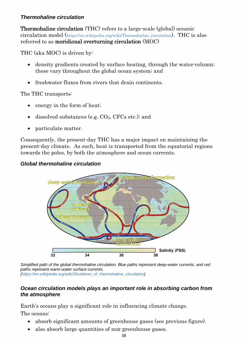
Global thermohaline circulation

Simplified path of the global thermohaline circulation. Blue paths represent deep-water currents, and red paths represent warm-water surface currents. (https://en.wikipedia.org/wiki/Shutdown_of_thermohaline_circulation)

Ocean circulation models plays an important role in absorbing carbon from the atmosphere

Earth’s oceans play a significant role in influencing climate change.

The oceans:

absorb significant amounts of greenhouse gases (see previous figure).

also absorb large quantities of non-greenhouse gases.

39

absorb heat from the atmosphere.

Watch the video on the role of ocean circulation in absorbing carbon from the

atmosphere at https://climate.nasa.gov/climate_resources/156/.

The Atlantic Meridional Overturning Circulation

With respect to moderating Earth’s climate, the Atlantic Meridional

Overturning Circulation (AMOC) is a crucial element of Earth’s climate

control systems. The so-called Gulf Stream is a component of the AMOC.

The Gulf Stream carries warm water from the Gulf of Mexico and

Florida to the vicinity of Greenland where it cools and then sinks to 100

metres or more.

Whilst moving northward surface waters absorb CO2 and other gases –

whilst in the vicinity of Greenland, the absorbed gases sink together

with the cooling water.

The removal of these gases on Earth’s climate is significantly reduced

because they remain in the deep ocean for years and even decades.

The cold water at depth then moves south to the tropics again, and the

cycle is repeated.

The AMOC draws greenhouse gases and heat deep into the Atlantic

Ocean, thereby helping to alleviate early effects of carbon emissions.

Between 2006 and 2016, 25% of anthropogenic CO2 emissions and 90%

of additional warming due to the enhanced greenhouse effect was

absorbed in the oceans. But how long can this be sustained?

However, as the ocean warms, circulation will slow-down, thereby

making it less effective at drawing CO2 and especially heat out of the

atmosphere (https://climate.nasa.gov/news/2598/nasa-mit-study-evaluates-efficiency-of-

oceans-as-heat-sink-atmospheric-gases-sponge/).

Presently, excess heat from climate change, and chemical pollutants and

greenhouse gases are being “buried” in the deep North Atlantic Ocean.

Eventually some of the CO2 and other dissolved gases will circulate back

to the tropics and be released into the atmosphere. When and how much CO2 are we talking about?

Scientists have used chlorofluorocarbons (CFCs) to study ocean circulation.

The rationale is that CFCs are a “passive tracer” and can be readily assayed in

sea water – their concentrations are a proxy to the concentration of dissolved

CO2 etc. The figure below shows the concentration of CFCs in the entire

Atlantic Ocean.

40

Concentration of CFCs in the Atlantic Ocean (https://climate.nasa.gov/news/2598/nasa-mit-study-evaluates-efficiency-of-oceans-as-heat-sink-atmospheric-gases-sponge/)

In the above figure, note the high concentrations of CFCs below a depth of

1000 metres in the vicinity of Greenland, despite that the ocean is

significantly deeper between latitudes ~10 °N and 30 °N.

? Future collapse of Atlantic Meridional Overturning Circulation

There are (possibly) conflicting data and interpretations about the future

collapse, slow-down or speed-up of the Gulf Steam and the AMOC

(https://en.wikipedia.org/wiki/Shutdown_of_thermohaline_circulation).

In theory, rapid melting of the Greenland icecap may be slowing-down the

AMOC due to an ingress of cold freshwater making the ocean less saline and

thereby slowing-down the rate of cold water sinking in the North Atlantic

Ocean.

However, studies by NASA and others since 2000 indicate that the AMOC had

not slowed down, and if anything, may have sped-up in the years leading up to

2010. Yet other studies seem to indicate a slow-down of the AMOC during the

20th Century. Clearly the science is complicated and requires a very holistic

and objective analysis (very easy to say!).

As seen from velocity data in the figure below, in the decade between May

1992 and June 2002, the flow of ocean currents south of Greenland and

Iceland had slowed down considerably. These velocity data may signal the

beginning of the shut-down of the AMOC.

41

Trend of velocities of ocean currents derived from the NASA Pathfinder altimeter data from May 1992 to June 2002. Ocean currents have slowed almost 6 m/s near Greenland and Iceland (https://en.wikipedia.org/wiki/Shutdown_of_thermohaline_circulation)

The slowing of the Gulf Stream and related currents in the North Atlantic

Ocean may involve:

Less warm water entering the North Atlantic leading to less

evaporation.

Less evaporation would lead to lower salinities in surface waters.

Lower salinities in surface waters would cause less sinking of water

(containing high concentrations of dissolved CO2).

Ironically, global warming might lead to a shut-down of the AMOC which

would cause a rapid cooling of the North Atlantic Ocean, and this would lead

to cooling in Europe and the eastern seaboard of North America.

The Intergovernmental Panel on Climate Change (ICPP) is a globally funded

institute that attempts to synthesise the vast body of research that is

published annually on climate change and related matters. Until now the

ICPP has operated on the assumption that the AMOC is stable and will not

collapse.

This notion has recently been challenged by the outcome of research from the

Scripps Institute of Oceanography at the University of California, San Diego

(https://scripps.ucsd.edu/news/climate-model-suggests-collapse-atlantic-circulation-possible).

Computer simulations by the institute’ researchers indicated that AMOC is

likely to collapse, or to use a less dramatic language, “switch to a different state of equilibria” some 300 years after the atmospheric CO2 level is double

its 1990 level.

42

Assuming the present rate of increase of atmospheric CO2, when will the concentration of CO2 reach double its 1990 level?

North Atlantic Ocean cooling scenario following collapse of AMOC approximately 300 years after the atmosphere attains ~700 ppm CO2 (https://scripps.ucsd.edu/news/climate-model-suggests-collapse-atlantic-circulation-possible)

In the San Diego researchers’ paper, the hypothesized outcomes of a collapse

of the AMOC are:

spread of sea ice.

North Atlantic surface temperatures to drop by ~2.4 °C.

surface air temperatures in NW Europe to drop by up to 7 °C.

A southward shift in the tropical rain belts in the Atlantic Ocean.

What would be the global socio-economic and geopolitical consequences of such a scenario eventuating?

The 2004 Film: The Day After Tomorrow

The 2004 Hollywood film, “The Day after Tomorrow” is based around the

future collapse of the AMOC. The film grossly exaggerated a scenario

whereby Earth (at least North America) is “snap frozen” as a result of changes

to AMOC.

An image promoting the film “The Day after Tomorrow” that sensationalised many aspect of a potential shut-down of the AMOC (http://adamjgblog.blogspot.com.au/2010/12/analysis-of-day-after-tomorrow.html)

43

The AMOC at the peak of the last Ice Age (~20 ka)

Read all about “The Once and Future Circulation of the Ocean” at

http://www.whoi.edu/oceanus/feature/the-once-and-future-circulation-of-the-ocean.

Upper: The ocean's overturning circulation carries a vast amount of heat northward, warming the North Atlantic region. It also generates a huge volume of cold, very saline water called North Atlantic Deep Water – a great mass of water that flows southward, filling-up the deep Atlantic Ocean basin and eventually spreading into the deep Indian and Pacific oceans (http://www.whoi.edu/oceanus/feature/the-once-and-future-circulation-of-the-ocean)

Lower: Palaeo-oceanographers have found evidence for very different patterns of ocean circulation in the past. At ~ 20 ka, waters in the North Atlantic sank only to intermediate depths and spread to a far lesser extent. When that occurred, the climate in the North Atlantic region was generally cold and more variable. (Illustration by E. Paul Oberlander, Woods Hole Oceanographic Institution)

44

Anthropogenic activities affect climate conditions

Explain the enhanced greenhouse effect

The enhanced greenhouse effect describes the extra “mankind-induced”

(anthropogenic) greenhouse effect. The proposition is that humanity

continues to produce greenhouse gases over and above the levels that would

have been produced by natural causes alone. The figure below indicates

actual measured CO2 concentrations (ppm) each month between 1958 and

2005.

Time (year) versus monthly average C02 concentration in ppm (http://blogs.edf.org/climate411/2007/06/21/human_cause-2/)

Regular and accurate measurement of atmospheric CO2 commenced in the

1950s.

The zig-zag pattern of the atmospheric concentration of CO2 is due to seasonal

fluctuations in plant activity – mostly from deciduous plants in the Northern

Hemisphere.

The graph indicates that the level of CO2 in the atmosphere has increased

from (at least) the year 1958 into the 2000s. If the increase were due to

mankind’s burning of fossil fuel, we should expect a concomitant decrease in

the concentration of O2. According to the stoichiometry of the reaction below,

which is based on the combustion of methane, but in principle stands for the

combustion of any fossil fuel.

Molecular models showing the combustion of methane to produce the greenhouse gases CO2 and water (https://en.wikipedia.org/wiki/Combustion)

45

2011 mole fraction of CO2 in the troposphere (https://en.wikipedia.org/wiki/Carbon_dioxide_in_Earth%27s_atmosphere)

Time (year) versus monthly average C02 concentration in ppm, with O2 concentration (http://blogs.edf.org/climate411/2007/06/21/human_cause-2/)

46

Consider the figure above that shows significantly higher levels of CO2 in the Northern Hemisphere during May 2011 when compared to October 2011. Why is that so? (there are likely to be several good answers to this question)

Describe anthropogenic activities that are changing the levels of greenhouse gases

Anthropogenic activities that have increased the level of greenhouse gases

include:

Burning of fossil fuels that produces largely CO2

Deforestation for urban and agricultural development that releases CO2

through burning of biomass waste and decay

Mining and industrial processes that manufacture greenhouse-inducing

gases (e.g. CH4, NO2)

Agricultural practices that till and degrade the soil’s capacity to absorb

and store carbon

Large-scale world-wide livestock husbandry that produces large

quantities of CH4.

World energy consumption since 1820

World capita energy consumption since 1820 (https://www.treehugger.com/fossil-fuels/world-energy-use-

over-last-200-years-graphs.html)

47

CO2 emissions from the major emitting countries

CO2 emissions since 400 ka

Atmospheric CO2: at 406.94 ppm, 2017 levels are the highest in 650,000 years.

World map of CO2 emissions

Global anthropogenic CO2 emissions by “edimbukvarevic” (https://wattsupwiththat.com/2015/10/04/finally-

visualized-oco2-satellite-data-showing-global-carbon-dioxide-concentrations/)

48

Natural versus anthropogenic methane

Role of animal farts in global warming (https://www.livescience.com/52680-the-role-of-animal-farts-in-global-warming-infographic.html)

49

Please read an article by Dan Bell on “The methane makers” at http://news.bbc.co.uk/2/hi/uk_news/magazine/8329612.stm

Some pertinent statistics – on Earth there are approximately

7 billion humans

(only) 1.4 billion cattle

(only) 1 billion sheep

(only) 1 billion pigs

Source of data: https://www.economist.com/blogs/dailychart/2011/07/global-livestock-counts

Refer to the “pertinent statistics” (above) and information from the previous figure. World-wide, how many tonnes of methane are produced by humans and their domesticated cattle, sheep and pigs per year? How much CO2 “green-house equivalent” is this amount of methane?

Roughly what proportion of livestock methane emissions are derived from industrialised western countries, i.e. countries with a high HDI?

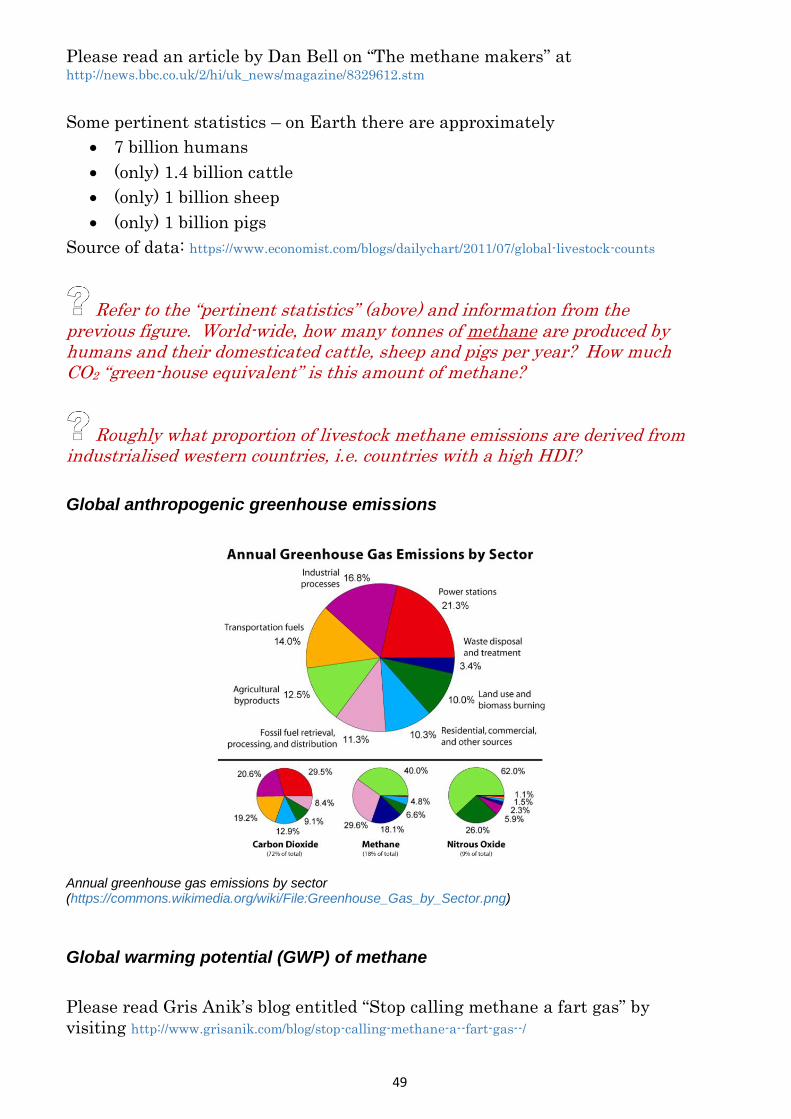
Global anthropogenic greenhouse emissions

Annual greenhouse gas emissions by sector (https://commons.wikimedia.org/wiki/File:Greenhouse_Gas_by_Sector.png)

Global warming potential (GWP) of methane

Please read Gris Anik’s blog entitled “Stop calling methane a fart gas” by

visiting http://www.grisanik.com/blog/stop-calling-methane-a--fart-gas--/

50

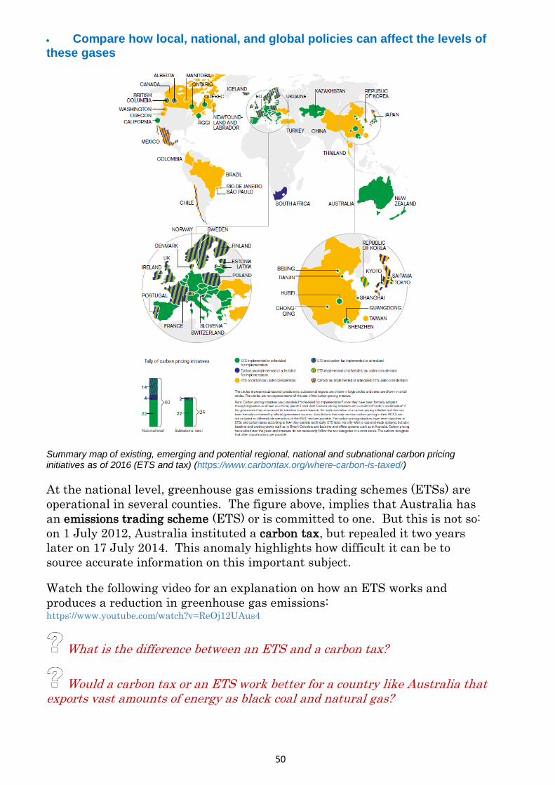
Compare how local, national, and global policies can affect the levels of these gases

Summary map of existing, emerging and potential regional, national and subnational carbon pricing initiatives as of 2016 (ETS and tax) (https://www.carbontax.org/where-carbon-is-taxed/)

At the national level, greenhouse gas emissions trading schemes (ETSs) are

operational in several counties. The figure above, implies that Australia has

an emissions trading scheme (ETS) or is committed to one. But this is not so:

on 1 July 2012, Australia instituted a carbon tax, but repealed it two years

later on 17 July 2014. This anomaly highlights how difficult it can be to

source accurate information on this important subject.

Watch the following video for an explanation on how an ETS works and

produces a reduction in greenhouse gas emissions: https://www.youtube.com/watch?v=ReOj12UAus4

What is the difference between an ETS and a carbon tax?

Would a carbon tax or an ETS work better for a country like Australia that exports vast amounts of energy as black coal and natural gas?

51

International agreements on climate change and greenhouse gas emissions

At an international level, the International Panel on

Climate Change (IPCC) is a scientific body established

with the support of the United Nations to provide

impartial and objective advice regarding climate

change. The purpose of the IPCC is to assess scientific

information relevant to:

Human-induced climate change

Impacts of human-induced climate change

Options for adaptation and mitigation

What is the Kyoto Protocol?

There have been several international meetings on

climate change. One of the most recent was a meeting

in Paris. In 2017 US president Donald Trump

announced that he would withdraw USA would from

the “Paris Agreement”

What is the Paris Agreement?

What exactly does Donald Trump mean when he says he is “withdrawing from Paris”?

The newspaper clip is from page 1 of The Australian on

2 November 2017. However, almost every day there

are newspaper articles on international agreements,

climate change, greenhouse gas “targets”, renewable

energy schemes and the escalating cost of electricity in

Australia. Amongst other things we are told that

South Australia has the highest cost of electricity in the

world.

Read the newspaper article. Given that ~50% of Australia’s population are willing to pull-out of the Paris Agreement to secure cheaper electricity, how will

that fact impact on Australia’s ability to deliver reduced greenhouse gas emissions beyond the next Federal election?

A state-based carbon tax or ETS?

52

The Premier of South Australia, Jay Wetherill, has suggested that the states

of Australia, independent of the Federal Government of Australia, should “go

it alone” on an emissions trading scheme. This approach has been critisised

by the Prime Minister and others (http://www.sbs.com.au/news/article/2016/12/08/factbox-

carbon-taxes-and-emission-trading-schemes-around-world)

Would a states-impose ETS work? If so how? Is there anything similar elsewhere in the world?

Presently the states of Australia all have different greenhouse gas emission targets. Use the internet to research these. Will such an approach lead to complete chaos in the electricity market, or is such an approach necessary given the absence of Commonwealth leadership, and lack of support (i.e. the newspaper article) from the Australian population to reduce greenhouse gas emissions?

Local government response to climate change

How are local governments and communities in South Australia responding to minimize emissions of greenhouse gases?

53

Explain how carbon is stored in Earth’s systems over a variety of time-scales.

Because Earth is dynamic, carbon is cycled through Earth’s four systems – the

geosphere, biosphere, atmosphere and hydrosphere. This process is called the

carbon cycle.

Diagrammatic representation of the carbon cycle. Black numbers, in Gt of carbon (109 tonnes C) as around the year 2004. Purple numbers represent the quantities of carbon flux per annum. As reported in this diagram, “sediments” refers to the most shallow sediments that have been deposited during a year – the term does not include carbon within coal, kerogen or carbonate rock (https://simple.wikipedia.org/wiki/Carbon_cycle)

The caption to the above figure above refers to kerogen. What is kerogen?

Long term storage of carbon (slow carbon cycle)

Carbon has been cycled through Earth’s four systems since the advent of life

at ~ 4.1 Ga. During the Precambrian, organic carbon from prokaryotes was

preserved as dispersed organic matter (DOM) within sediments that were

later lithified, and the DOM converted to graphite.

Carbon stored as petroleum

Earth’s oldest oil (~ 1.6 Ga) is from the McArthur Basin in the Northern

Territory.

54

Onshore sedimentary basins prospective for petroleum and/or coal (http://www.ga.gov.au/about/projects/resources/onshore-petroleum)

These oils are sourced from organic rich shales deposited in an intra-cratonic

basin during the Paleoproterozoic and Mesoproterozoic. Note: The McArthur

basin also has very considerable potential for unconventional oil and gas

potential (i.e. shale gas and shale oil).

Small quantities of oil and gas has been discovered in Australia’s Cambrian

Basins (see above figure). However, the bulk of Australia’s oil and gas is

sourced from younger sediments of Palaeozoic (Warburton basin), Palaeozoic–

Mesozoic (Cooper Basin), Mesozoic (Eromanga Basin) and Cenozoic (Gippsland

Basin) age. Oil and gas from the offshore North west Shelf of western

Australia are sourced predominantly from Mesozoic sedimentary rock.

The giant oil reserves of the Middle East are primarily derived from

carbonate-rich sediments and shales of Mesozoic age.

Carbon stored as coal

The first vascular land plants evolved during the Silurian Period.

Evolutionary botanists consider Baragwanathia ssp. (~427–393 Ma), first

discovered in eastern Victoria to be the first true land plant.

During the Silurian and Devonian periods, plants were evidently not as

widespread as from the Carboniferous onwards when suitable environments

resulted in widespread deposition of peat forming environments. Indeed, the

Carboniferous Period is named for the shear bulk of the carbon that was

captured from the atmosphere into the subsurface to form coal measures.

55

Carboniferous coal measures are widespread and formed across the globe – in

Australia, Africa, North America and Eurasia. Note: in North America, the

Carboniferous Period is subdivided between the older Mississippian Subperiod

and the younger Pennsylvanian Subperiod.

Peat formation and coal formation continued on all continents throughout the

Mesozoic and Cenozoic eons; this includes Antarctica where coal formation

was important during the early Cenozoic (~55–35 Ma) when Antarctica was

ice-free, connected to Australia and at a more northern latitude. Coal in

Antarctica outcrops in coastal sections and in the Transantarctic Mountains.

What other places in the world have huge Cenozoic coal deposits?

Use Google Earth to locate the Transantarctic Mountains. What other features in Antarctica can be resolved using Google Earth?

The components of the carbon cycle can be classified as either carbon pools or

carbon fluxes.

The figure below is yet another representation of the carbon cycle. The fast

carbon cycle comprises those components of the carbon cycle that move carbon

between pools within the timescale of hours, day, and years.

Another schematic representation of the annual carbon cycle by the University of New Hampshire (http://globecarboncycle.unh.edu/diagram.shtml). Note: one petagram (Pg) = one gigatonne (Gt)

Based on the figure above, carbon pools include:

plants (560 Gt)

56

atmosphere (750 Gt)

soils (1500 Gt)

fossil fuels, i.e. both petroleum and coal (4000 Gt)

the oceans and other bodies of water (38,000 Gt)

Earth’s crust (100,000,000 Gt)

Carbon fluxes include:

volcanoes (0.1 Gt) → atmosphere

burial within oceans (0.1 Gt) → shallow sediments

rivers (0.8 Gt) → ocean

deforestation etc. (0.9 Gt) → atmosphere

burning fossil fuels (6 Gt) → atmosphere

litter-fall (60 Gt) → soil

soil respiration (60 Gt) → atmosphere

plant respiration (60 Gt) → atmosphere

ocean loss (90 Gt) → atmosphere

ocean uptake (92 Gt) → oceans

photosynthesis (120 Gt) → plants

How does the data in the carbon cycle diagram by the University of New Hampshire compare with data in the figure published by Wikipedia?

The data in the carbon cycle figure by the University of New Hampshire has most probably been reviewed by peers. It was drafted in the year 2007. Use the internet to check the validity of some or all of these data – both for pools and for fluxes. What are your generalized findings?

Prior to deforestation and the burning of fossil fuels, the atmosphere contained ~560 Gt of carbon (http://globecarboncycle.unh.edu/CarbonPoolsFluxes.shtml). When did large-scale deforestation begin? And when did the widespread burning of fossil fuels commence?

57

Geo-statistics from a paper by Philip Abelson

Some geo-statistics from a 1978 paper by Philip Abelson Organic matter in the Earth’s crust (Annual Review of Earth and Planetary Science 1978, vol. 6, pp.

325–351):

There are ~ 830 x 1012 kg of living matter on Earth’s land surface and in

the oceans.

Annual production of living matter is ~ 78 x 1012 kg.

An estimate of the total production during Earth’s history is between 5 x

1021 and 5 x1022 kg.

Most of the above figures for total annual production return to the

atmosphere as CO2.; however, it is estimated that ~19 x 1018 kg of

organic or elemental carbon has been preserved within the crust since

life evolved.

Most of the carbon within Earth’s crust is within sedimentary rocks – some is

diluted and dispersed within sediments (dispersed organic matter), and some

becomes concentrated as coal or petroleum. However, as Abelson pointed-out

only about 1 part in 1000 that is produced annually is not converted to CO2 and is preserved in the geological record.

Extraterrestrial sources of carbon

Presently, Earth’s magnetic field and its atmosphere, particularly the

thermosphere protects Earth’s biosphere from small bolides and dangerous

cosmic radiation. Without this protection complex terrestrial life would not be

possible. However, meteorites that do reach Earth’s surface contain small

quantities of “organic-like” carbon. Possibly more than 20% of carbon in the

universe may be in the form of “organic-like” polyaromatic hydrocarbons

(PAHs); in 2014 NASA launched a project to track PAHs in the universe.

We have previously discussed the Late Heavy Bombardment (LHB, ~4 Ga)

when an unusual large number of asteroids collided with Earth and other

terrestrial planets. Although the concentration of carbon as PAHs in

meteorites is very small, the sheer volume of meteorite bombardment during

the LHB, would have bought significant amounts of “organic-like” carbon to

Earth early in its history.

58

Climate change affects Earth systems

Discuss the effects of climate change on Earth systems

Methane clathrates

In Topic 2 (Earth’s Resources) we discussed methane clathrates, their

formation and global distribution. These hydrocarbons (mostly methane) are

an enormous untapped source of energy. However, they are arguably pose the

greatest threat to Earth’s climate, especially in a scenario of “run-away” global

warming should Earth’s permafrost continue to melt.

Some numbers:

methane is 24 times more potent a greenhouse gas than CO2

compression of methane in clathrates is enormous – one m3 of clathrate

taken from the deep ocean’s surface releases 164 m3 of methane

Source: http://www.planetextinction.com/planet_extinction_clathrates.htm

Permafrost – definition

Permafrost is permanently frozen ground that remains at or below 0 °C for at

least two years. There are four Earth environments where methane

clathrates occur (http://geology.com/articles/methane-hydrates/):

sediment and sedimentary rock units below Arctic permafrost

sedimentary deposits along continental margins

deep water sediments of lakes and seas

under Antarctic ice

Distribution of Northern Hemisphere permafrost by NASA’s Scientific Visualization Studio. White = glacier; dark purple = continuous permafrost; medium purple = discontinuous permafrost; lilac = isolated permafrost (https://svs.gsfc.nasa.gov/3511)

59

Distribution of permafrost in Asia and Siberia. Continuous permafrost from a 2010 research paper by Robin Grayson “Asian ice shields and climate change” (World Placer Journal 2010, vol. 10, pp. 21–45 (>90% area) in darkest blue; discontinuous permafrost (50–90%) in medium blue; sporadic permafrost (10–50%) in pale blue; Isolated Permafrost (<10%) in faintest blue. (https://www.researchgate.net/figure/284477388_fig2_Figure-3-distribution-of-permafrost-in-Asia-and-Siberia-Continuous-Permafrost-90)

Is the Tibetan Plateau still rising? If so, were it not for “Global Warming” should we expect the areas of permafrost in Tibet and far-western China to grow?

Thawed surface of permafrost on the tundra, Taymyr Peninsular, far northern Siberia (https://www.britannica.com/science/permafrost)

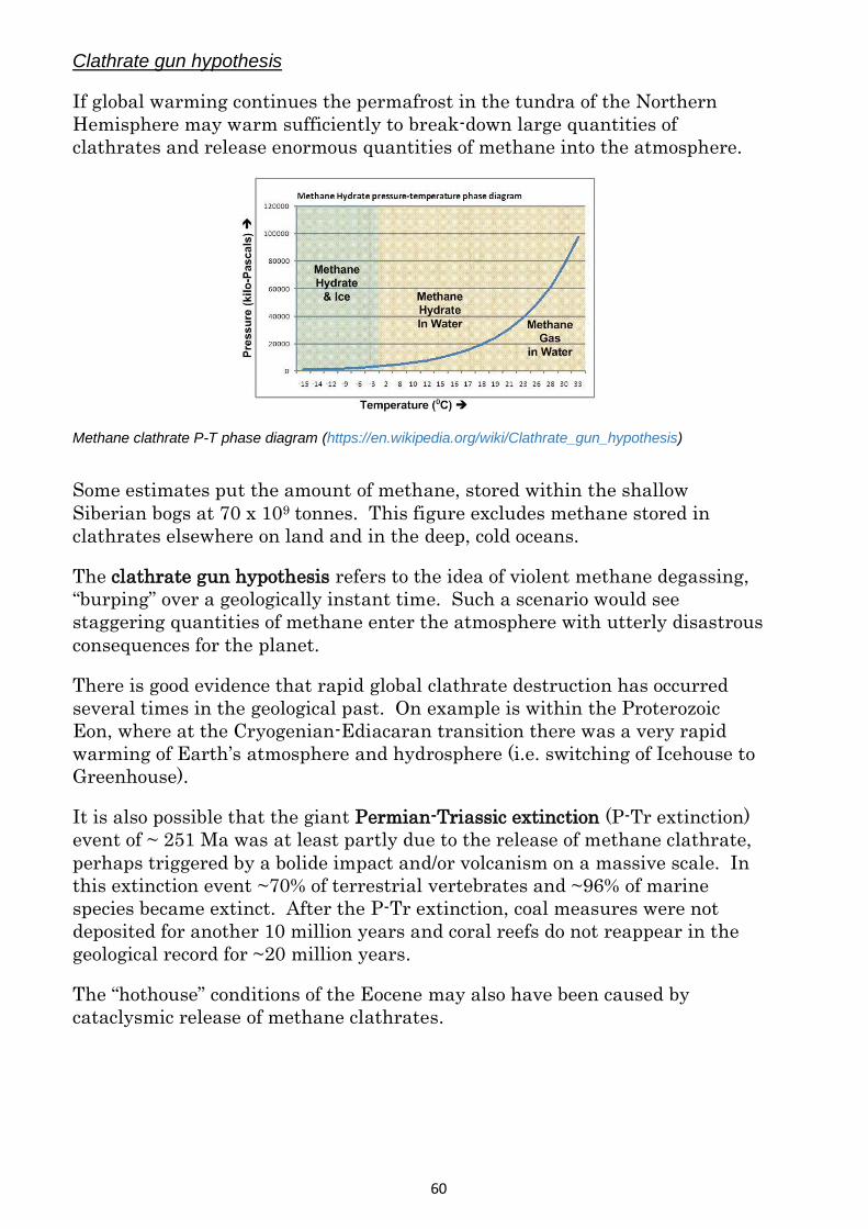
60

Clathrate gun hypothesis

If global warming continues the permafrost in the tundra of the Northern

Hemisphere may warm sufficiently to break-down large quantities of

clathrates and release enormous quantities of methane into the atmosphere.

Methane clathrate P-T phase diagram (https://en.wikipedia.org/wiki/Clathrate_gun_hypothesis)

Some estimates put the amount of methane, stored within the shallow

Siberian bogs at 70 x 109 tonnes. This figure excludes methane stored in

clathrates elsewhere on land and in the deep, cold oceans.

The clathrate gun hypothesis refers to the idea of violent methane degassing,

“burping” over a geologically instant time. Such a scenario would see

staggering quantities of methane enter the atmosphere with utterly disastrous

consequences for the planet.

There is good evidence that rapid global clathrate destruction has occurred

several times in the geological past. On example is within the Proterozoic

Eon, where at the Cryogenian-Ediacaran transition there was a very rapid

warming of Earth’s atmosphere and hydrosphere (i.e. switching of Icehouse to

Greenhouse).

It is also possible that the giant Permian-Triassic extinction (P-Tr extinction)

event of ~ 251 Ma was at least partly due to the release of methane clathrate,

perhaps triggered by a bolide impact and/or volcanism on a massive scale. In

this extinction event ~70% of terrestrial vertebrates and ~96% of marine

species became extinct. After the P-Tr extinction, coal measures were not

deposited for another 10 million years and coral reefs do not reappear in the

geological record for ~20 million years.

The “hothouse” conditions of the Eocene may also have been caused by

cataclysmic release of methane clathrates.

61

Sonar image of methane plume discovered of the US east coast. Scientists estimate there could be ~30,000 similar plumes worldwide (http://www.bbc.com/news/science-environment-28898223)

Organic carbon stored in permafrost terrane

Large quantities of soil organic carbon (SOC) are also stored in permafrost

terranes (http://www.permafrostcarbon.org/Cquantity.html). Should Earth’s climate

become warmer, and permafrost terranes thaw, SOC may break-down and

oxidise thereby giving rise to additional CO2 flux into the atmosphere.

Organic carbon in soils

Excluding permafrost, enormous amounts of organic matter and organic

carbon are stored in conventional soils. Climate change and global warming,

exacerbated by agricultural practices would all be expected to have some

impacts on the globe’s soils. The electronic Footprints Newsletter

(http://www.planetextinction.com/Newsletter/footprints_3_Dec06.html) makes many claims

including:

“Altogether there is 300 times as much carbon trapped in the soils as we release each year from burning fossil fuel”

Try and verify or disprove these assertions for yourself. How much organic matter/organic carbon is stored in the Earth’s soils? What happens to the organic matter component of soils once the soils degrade and erode?

Intense farming practices, especially broad-acre farming has removed large

quantities of carbon from soils. This is especially worrying because it takes

thousands of years for soils to form.

A recent study on the effects of environmental warming on the stability of

carbon in mid-latitude forest soils found that:

“once warming reaches a certain point, these natural biological factors kick in and can lead to a runaway, and potentially unstoppable, increase in warming”.

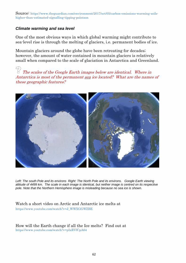
62

Source: https://www.theguardian.com/environment/2017/oct/05/carbon-emissions-warming-soils-

higher-than-estimated-signalling-tipping-pointson

Climate warming and sea level

One of the most obvious ways in which global warming might contribute to

sea-level rise is through the melting of glaciers, i.e. permanent bodies of ice.

Mountain glaciers around the globe have been retreating for decades;

however, the amount of water contained in mountain glaciers is relatively

small when compared to the scale of glaciation in Antarctica and Greenland.

The scales of the Google Earth images below are identical. Where in Antarctica is most of the permanent sea ice located? What are the names of these geographic features?

Left: The south Pole and its environs Right: The North Pole and its environs. Google Earth viewing altitude of 4499 km. The scale in each image is identical, but neither image is centred on its respective pole. Note that the Northern Hemisphere image is misleading because no sea ice is shown.

Watch a short video on Arctic and Antarctic ice melts at

https://www.youtube.com/watch?v=J_WWXGGWZBE

How will the Earth change if all the Ice melts? Find out at https://www.youtube.com/watch?v=pIxRVfCpA64

63

Sea level rises in the last 25 years

August 2017 is the 25th anniversary of the systematic monitoring of global sea

level data by NASA using satellites. Despite considerably variations across

the globe, over those 25 years, the “average” sea surface height has risen ~7

cm.

Global sea level data by NASA. Upper: October 1993. Lower: July 2017

(https://www.nasa.gov/feature/jpl/25-years-of-global-sea-level-data-and-counting)

64

Melting of sea ice versus continental ice sheets

Just the “Tip of the iceberg”

H2O has a number of unusual properties – we have already discussed water’s

unusually high specific energy – one other important properties is the density

differential between liquid water and ice.

Unlike most other substances, the solid form of H2O, ice is less dense than its

liquid counterpart. As a consequence, icebergs float with most of the mass

below the water mark, and only a small fraction above the water mark above

the water mark.

Antarctica

Vertical cross-section through Antarctica reveals that, amongst other things, the East Antarctic ice sheet is considerably thicker than its counterpart in West Antarctica (http://discoveringantarctica.org.uk/wp-content/uploads/2015/11/a_1.4_continent_cross_section_ab_2x.png)

Cartoon showing contrasting aspects of ice accumulation a, ice sheet movement and icebergs “calving” in Antarctica and Greenland (https://lima.nasa.gov/antarctica/)

65

Some interesting numbers:

The density of pure water (by definition) is 1.0 g/cm3 (= 1000 kg/m3)

Density of seawater is 1025 kg/m3

As described by the Archimedes’ principal, typically one-tenth of the

volume of an iceberg is above the water’s surface.

With respect to sea level rise, given the above numerical values, should we be more concerned about the melting of sea ice or continental ice?

What is the present-day volume of ice in the form of continental ice, sea ice and alpine glacial ice?

Other impacts of climate change

Rainfall precipitation

Based on a medium emissions scenario, modelling of global rainfall patterns

suggest that all of Australia (with the possible exception of Tasmania) will

have significantly lower rainfall by the year 2100.

Projected change in annual average precipitation between 200 and 2100 based on SRES A1B emissions

scenarios. (https://en.wikipedia.org/wiki/Physical_impacts_of_climate_change)

Climate change feedback

If global warming continues, additional water vapour will be added to the

atmosphere, which in turn leads to additional warming, which in turn leads to

further warming. This process is called a positive feedback.

Can you think of any other positive feedbacks related to climate change?

Rainforest shrinking

66

The projected rainfall map suggests there will be diminished rainfall in places

where there are presently rainforests (i.e. Congo basin, southern Brazil, NE

coastal Queensland).

What implications will this have for rainforest sustainability, biodiversity and the amount of global photosynthesis?

Prior to ~10 ka, vegetation belts/zones were able respond to climate change, and adapt as well as “migrate” across landmasses and into new environmental niches. Suggest a reason why that is no longer possible?

Instability of landforms

The projected rainfall map suggests an increase in precipitation across

Canada, Siberia, and northern Europe by the year 2100.

If increase rainfall occurs across the far Northern Hemisphere, and this occurs concomitantly with the melting of permafrost, what consequences would it have on the stability of the landscape generally?

Acidification of oceans

Another indicator of climate change and the rise of CO2 in the ecosystem is the

amount of CO2 dissolved in the world’s oceans.

Changes in dissolved carbon dioxide in the worlds oceans between the 1980s and the early 2000s (https://www.epa.gov/climate-indicators/climate-change-indicators-ocean-acidity)

67

CO2 concentrations in the oceans have been steadily increasing along with

atmospheric CO2. Although the dissolution of CO2 in the oceans helps slow-

down its build-up in the atmosphere – it causes immense problems of its own.

Dissolved in water CO2 becomes carbonic acid. Therefore, as CO2

concentration in the oceans has increased, so too has their acidity.

Air-sea exchange of carbon dioxide (https://en.wikipedia.org/wiki/Carbon_sink)

The above figure is a schematic that summaries the part of the carbon cycle

related to the exchange of CO2 between the atmosphere, oceans and recent

shallow sediments. In this figure, a carbon sink would be the shallow

“reactive” sediments that sequester both organic and inorganic carbon.

What mineral(s) commonly formed throughout the world’s oceans are pH sensitive in terms of their stability?

What implications does the increasing acidity of the world’s oceans have on the ecological functioning of coral reefs? And Australia’s Great Barrier Reef?

Other than considerations of oceanic acidity, what other climate change-related threats are likely to affect the Great Barrier Reef?

68

Natural carbon sequestration

Schematic summary illustrating components of the fast carbon cycle. Numbers refer to billions of tonnes per year. Yellow numbers are natural fluxes and red numbers are anthropogenic fluxes (https://en.wikipedia.org/wiki/Carbon_sink)

More detail of the carbon cycle (https://www.carboncyclescience.us/what-is-carbon-cycle)

69

Natural carbon sequestration is the process of moving carbon (as atmospheric

CO2) into the biosphere and eventually into the geosphere, or directly into the

geosphere.

How will climate change (global warming, sea level rises and changes in rainfall) impact on the fast carbon cycle?

Explore the potential risks and benefits of using geosequestration to reduce atmospheric levels of CO2

Carbon geosequestration

The term carbon geosequestration describes the capture and long-term storage

of CO2. The Parliament of Australia’s website provides an excellent summary

of several approaches to CO2 sequestration

(https://www.aph.gov.au/About_Parliament/Parliamentary_Departments/Parliamentary_Library/Bro

wse_by_Topic/ClimateChangeold/responses/mitigation/carbon)

Plant sequestration

The simplest way to sequestering CO2 could be to planting millions upon

millions of trees – but that approach has its many environmental end

economic limitations. Moreover, the carbon stored in plant biomass is part of

the fast carbon cycle, and is therefore likely to return to the atmosphere

within a century or even less.

What are the limitations of “tree planting” to sequester CO2 in the atmosphere?

Ocean sequestration, soil sequestration and mineral sequestration

There are several other (untested and risky) sequestration options including

ocean sequestration, soil sequestration and mineral sequestration which are

discussed in the Parliament of Australia website (see above).

Carbon geosequestration

Carbon geosequestration is the process of taking CO2 and storing it in deep

geological formations – this idea also goes by the name of carbon capture and

storage (CCS). CCS involves capturing CO2 at the point of emission. The CO2

would then be liquefied (a very energy intensive proposition!) and injected

under pressure into deep geological structure.

70

Hazelwood power station (Victoria) in full operation when it could produce ~25% of Victoria’s electricity requirements from burning brown coal (lignite) (http://reneweconomy.com.au/engie-flags-potential-closure-of-hazelwood-worlds-most-polluting-power-plant-26484/)

A more sophisticated way of reducing greenhouse gases might be to “scrub”

them from the exhaust chimneys of coal or gas-fired power stations. This is a

logical proposition: take for example the Hazelwood Power Station, in

Victoria’s Latrobe Valley, which was shut-down in March 2017. When fully

operational, it had a 1600 MW capacity and could produce ~5% of Australia

electricity demand. The down-side was that it produced ~ 5% of Australia’s

greenhouse gas emissions, making it one of the dirtiest and environmentally

nasty power stations in the developed countries, if not the world.

Reflecting on what we discussed in Topic 2 (Earth’s Resources) why was Hazelwood so polluting, and why will the remaining Latrobe Valley power generators remain very polluting with respect to CO2 emissions?

If power stations like Hazelwood could be retrofitted with “CO2 scrubbers”

part of the energy produced by the power station could be used to liquefy the

CO2 generated from burning coal and transport it to designated locations for

injection (sequestration) into deep “reservoirs”. Alternatively, new coal-fired

power plants could be built with carbon-scrubbers as an integral part of their

design.

Some geosequestration options (http://www.bigskyco2.org/geologic_css)

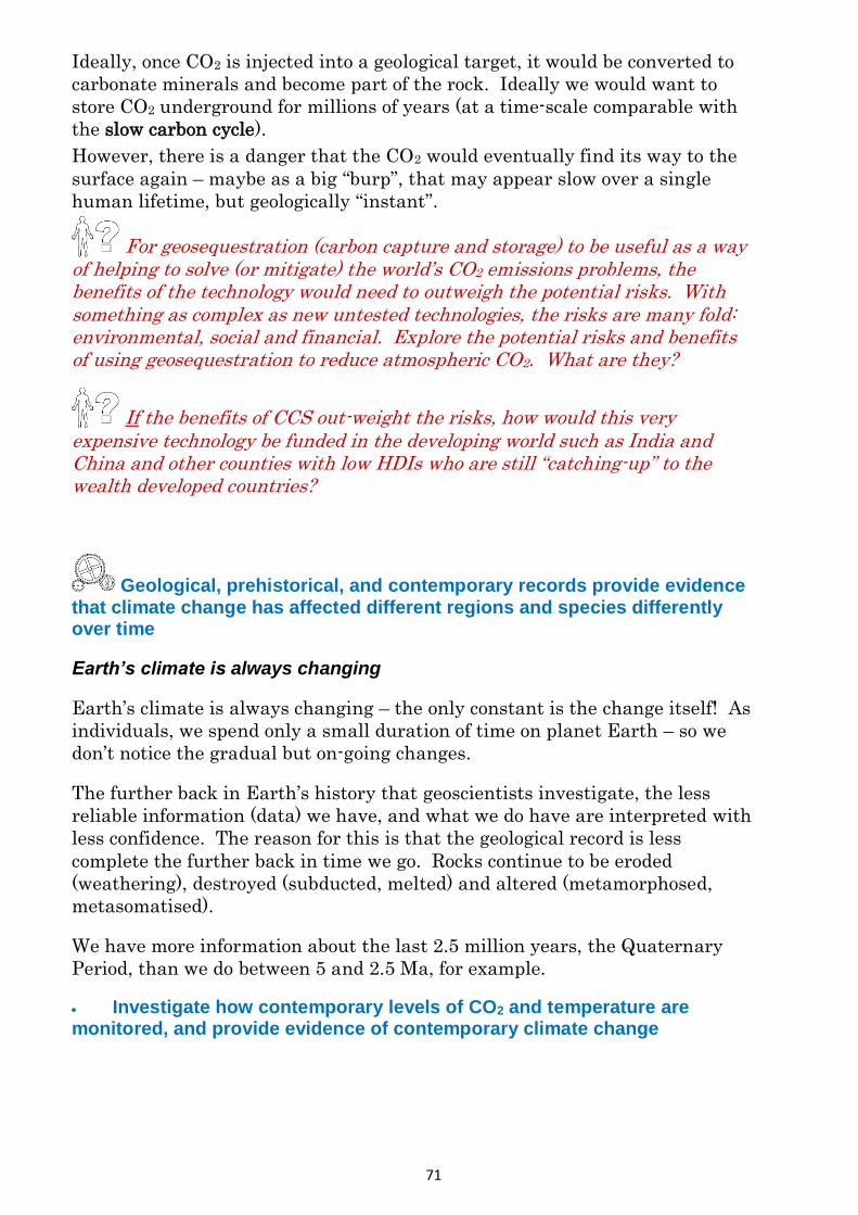
71

Ideally, once CO2 is injected into a geological target, it would be converted to

carbonate minerals and become part of the rock. Ideally we would want to

store CO2 underground for millions of years (at a time-scale comparable with

the slow carbon cycle).

However, there is a danger that the CO2 would eventually find its way to the

surface again – maybe as a big “burp”, that may appear slow over a single

human lifetime, but geologically “instant”.

For geosequestration (carbon capture and storage) to be useful as a way of helping to solve (or mitigate) the world’s CO2 emissions problems, the benefits of the technology would need to outweigh the potential risks. With something as complex as new untested technologies, the risks are many fold: environmental, social and financial. Explore the potential risks and benefits of using geosequestration to reduce atmospheric CO2. What are they?

If the benefits of CCS out-weight the risks, how would this very

expensive technology be funded in the developing world such as India and China and other counties with low HDIs who are still “catching-up” to the wealth developed countries?

Geological, prehistorical, and contemporary records provide evidence that climate change has affected different regions and species differently over time

Earth’s climate is always changing

Earth’s climate is always changing – the only constant is the change itself! As

individuals, we spend only a small duration of time on planet Earth – so we

don’t notice the gradual but on-going changes.

The further back in Earth’s history that geoscientists investigate, the less

reliable information (data) we have, and what we do have are interpreted with

less confidence. The reason for this is that the geological record is less

complete the further back in time we go. Rocks continue to be eroded

(weathering), destroyed (subducted, melted) and altered (metamorphosed,

metasomatised).

We have more information about the last 2.5 million years, the Quaternary

Period, than we do between 5 and 2.5 Ma, for example.

Investigate how contemporary levels of CO2 and temperature are monitored, and provide evidence of contemporary climate change

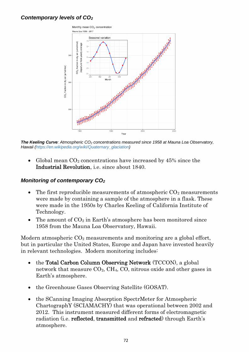
72

Contemporary levels of CO2

The Keeling Curve: Atmospheric CO2 concentrations measured since 1958 at Mauna Loa Observatory, Hawaii (https://en.wikipedia.org/wiki/Quaternary_glaciation)

Global mean CO2 concentrations have increased by 45% since the

Industrial Revolution, i.e. since about 1840.

Monitoring of contemporary CO2

The first reproducible measurements of atmospheric CO2 measurements

were made by containing a sample of the atmosphere in a flask. These

were made in the 1950s by Charles Keeling of California Institute of

Technology.

The amount of CO2 in Earth’s atmosphere has been monitored since

1958 from the Mauna Loa Observatory, Hawaii.

Modern atmospheric CO2 measurements and monitoring are a global effort,

but in particular the United States, Europe and Japan have invested heavily

in relevant technologies. Modern monitoring includes:

the Total Carbon Column Observing Network (TCCON), a global

network that measure CO2, CH4, CO, nitrous oxide and other gases in

Earth’s atmosphere.

the Greenhouse Gases Observing Satellite (GOSAT).

the SCanning Imaging Absorption SpectrMeter for Atmospheric

ChartographY (SCIAMACHY) that was operational between 2002 and

2012. This instrument measured different forms of electromagnetic

radiation (i.e. reflected, transmitted and refracted) through Earth’s

atmosphere.

73

Japan Aerospace Exploration Agency’s (JAXA) GOSat (Greenhouse

Gases Observing Satellite).

NASA’s Orbiting Carbon Observatory-2 (OCO-2) which launched in July

2014. OCO-2 does not directly measure CO2 concentrations – rather it

measures the electromagnetic radiation (sunlight) reflected of the CO2

molecules.

AIRS Mid-troposphere CO2, Version 5, July 2003(https://photojournal.jpl.nasa.gov/catalog/PIA10645)

https://photojournal.jpl.nasa.gov/catalog/PIA10645: “Although originally designed to measure atmospheric water vapor and temperature for weather forecasting, scientists working with the Atmospheric Infrared Sounder (AIRS) instrument on the NASA Aqua Spacecraft are now using AIRS to observe atmospheric carbon dioxide. Scientists from NASA, NOAA, ECMWF, UMBC, Princeton and CalTech using several different methods are measuring the concentration of carbon dioxide in the mid-troposphere (about 8 km above the surface). The global map of carbon dioxide above, produced by AIRS Team Leader Dr. Moustafa Chahine at JPL, shows that despite the high degree of mixing that occurs with carbon dioxide, the regional distribution can still be seen by the time the gases reach the mid troposphere. Climate modelers are currently using the AIRS data to understand the global distribution and transport of carbon dioxide and improve their models.”

View the short but excellent video on “Seasonal Changes in Carbon Dioxide”

at https://www.youtube.com/watch?v=EGQsBmzFM_g

74

Evidence of contemporary climate change

Some of the clearest evidence for present-day climate change include:

(Source: https://climate.nasa.gov/)

Global temperatures: 0.9 °C increase since 1880.

1884 global temperature anomalies

1943 global temperature anomalies

2016 global temperature anomalies

Visit climate https://climate.nasa.gov/ and study the global temperature anomaly

data.

Most recent global temperatures: 16 of the 17 warmest years have

occurred since 2001.

Sea levels: global average sea level has risen 178 millimetres over the

past 100 years.

Land ice: Earth’s polar ice sheets have been losing mass since at least

2002.

Sea ice: 2012 sea ice extent is the lowest in the satellite record.

75

1979 extent of Arctic sea ice

2012 extent of Arctic sea ice

2017 extent of Arctic sea ice

Source of images: https://climate.nasa.gov/

76

Explore how climate proxies are used to provide evidence of climate change

Climate proxies

Graph of reconstructed temperature (top – blue), CO2 (green-middle) and dust (red) from the Vostok

Station ice core since 420 ka (https://en.wikipedia.org/wiki/Quaternary_glaciation)

A “proxy” is a “substitute”. When referring to a “climate proxy” we refer to

information or data that can be used as reliable substitute for measured

temperatures in the geological past. Obviously we do not have a time-machine

to take us back to 420 ka, nor can we go back to 280 Ma to the Permian

glaciation. But we do have proxy data that have been carefully calibrated

against temperature.

In the ice core data from Vostok Station, scientists have used oxygen isotope

data derived from water (H2O). Specifically, they have used the ratio of two

oxygen isotopes (18O to 16O) as a palaeotemperature proxy. The oxygen isotope

system is well understood therefore confident correlations can be made

between palaeotemperatures and the oxygen isotope ratios expressed in the

geochemical notation of δ18O. The formula for δ18O is somewhat cumbersome;

however, put simply a high δ18O value means a high ratio of 18O to 16O.

18O is heavier than 16O and therefore water molecules (as part of ice) are

depleted in the heavier 18O. The is because it requires more energy to

evaporate a water molecule containing 18O than it does 16O.

77

In summary, in regard to polar ice:

There is less 18O during cold periods than during warm periods.

During warm periods 18O concentrations increase because there is more

thermal energy to evaporate “heavy” water (H2O containing 18O) from

the oceans and to move it via the atmosphere to the poles.

These processes that molecules containing isotopes of different mass are called

fractionation and are temperature dependent. For more on the determination

of temperature from ice core see https://www.scientificamerican.com/article/how-are-past-

temperatures/.

The data from Vostok Station is clear – there is an excellent correlation

between palaeotemperatures (as determined from proxy δ18O data) and CO2

concentrations from air bubbles trapped within the ice.

Palaeoclimates and glacial periods in Earth’s history

What is paleoclimatology?: https://www.ncdc.noaa.gov/news/what-paleoclimatology

We are presently living during an interglacial period of the most-recent ice

age. However, there have been at least five ice ages in earth’s history.

Please view the excellent summary at https://opentextbc.ca/geology/chapter/16-1-glacial-

periods-in-earths-history/

Precambrian ice ages

Timeline of glaciations, indicated in blue (https://en.wikipedia.org/wiki/Paleoclimatology)

There have been two (2) major glacial periods during the Precambrian:

Early Proterozoic (2.4–2.1 Ga): Huronian glaciation

Late Proterozoic (~700–650 Ma): Cryogenian glaciation (Earth’s most

intensive glaciation)

The glaciations of the Cryogenian Period are also known as the Snowball

Earth glaciations. It is now clear that the Snowball Earth glaciation

comprised at least two separate glaciations: The Sturtian glaciation at ~700

Ma and the Marinoan glaciation at 650 Ma, each lasting at least 20 million

years.

The Sturtian glaciation and the Marinoan glaciation are named after their

respective type-sections (where they were first discovered and/or described) in

78

South Australia. Glacial sedimentary rocks, especially tillite, are exposed in

the Adelaide Hills and the Flinders Ranges. The Sturtian glaciation is named

after Sturt Gorge, and the Marinoan glaciation is named after Marino Rocks

along the coast in Adelaide’s south.

Phanerozoic ice ages

Phanerozoic climate change (542 – 0 Ma) and oxygen isotope data (https://en.wikipedia.org/wiki/List_of_periods_and_events_in_climate_history)

There have been three (3) major glacial periods during the Phanerozoic:

Late Ordovician–Silurian: Andean-Saharan glaciation

Late Carboniferous–Permian: Karoo glaciation (Gondwanan glaciation)

Extent of Karoo glaciation during the early Permian, showing direction of ice flow. (http://nitishpriyadarshi.blogspot.com.au/2013/09/geological-evidences-of-ancient.html)

79

The Karoo glaciation (~360–260 Ma) only affected the southern hemisphere.

North America, for example, was unaffected because it was much closer to the

equator.

Polished and striated “pavement” at Hallett Cove, in Adelaide’s southern suburbs. The reddish brown rock is folded and uplifted Neoproterozoic siltstone (~600 Ma) abraded during the early Permian (~280 Ma). The striations that strike roughly NNW-SSE and other features indicate that the flow of ice was from the SSE towards the NNW, consistent with the ice-flow vectors on the map of Gondwana. (http://the-earth-story.com/post/104806454690/hallett-cove-600-million-years-of-history-at-a)

The present glaciation that affects Antarctica, Greenland and the Arctic

Ocean.

The Cenozoic (66 – 0 Ma)

Global temperature trends since the beginning of the Cenozoic at 66 Ma. Note that from the end of the Paleocene to the peak of the Pleistocene glaciation the global average temperature dropped by ~14 °C (https://opentextbc.ca/geology/chapter/16-1-glacial-periods-in-earths-history/)

As indicated in the above figure, Earth’s climate has been steadily cooling

since about 50 Ma. Geoscientists believe this is largely related to the

assembly of the Eurasian supercontinent, the Himalayan Mountains and the

vast Tibetan Plateau

80

The mechanism for this long-term cooling trend has been (and continues to be)

the enormous rate of erosion of the Himalayas, the concomitant weathering

and breakdown of silicate minerals and the withdrawal of CO2 from the

atmosphere (https://opentextbc.ca/geology/chapter/16-1-glacial-periods-in-earths-history/).

The figure above refers to the Antarctic Circumpolar Current. What is this current and why does its existence help trigger Antarctic glaciation at ~35 Ma?

The last 500,000 years

Global temperature data (based on O isotope data of forams) between 500 ka and the present (i.e. late Pleistocene). Note the periodicity of ~100,000 years for glacial cycles, that are marked with snowflake-star.

The data used to construct the curve in the figure above temperature proxy data derived from forams. What are forams?

The cyclicity of the global mean temperature data suggests that Earth is about to enter a colder and more glaciated period.

But hang on . . . . there is more to come!

81

The last 2000 years

Loehle Craig., 2007. A 2,000-year global temperature reconstruction on non-tree ring proxies. Energy and Environment 18, 1049–1058 ((http://www.drroyspencer.com/2009/07/how-do-climate-models-work/)

Icelandic and Norwegian Vikings were the first to discover North America and

Greenland. A Norse settlement at L’Anse aux Meadows (Newfoundland,

Canada) has been dated at between 990–1050 CE using radio carbon (14C)

methods (https://en.wikipedia.org/wiki/Norse_colonization_of_North_America). However, the

settlement evidently failed.

The Vikings also discovered Greenland and, commencing around 980 CE

settled its southern tip. However, by about 1430 CE the settlements had

failed and the remaining Vikings returned to Scandinavia.

The figure above refers to the Viking colonization of Greenland, and the “The Little Ice age”. Why did the Vikings’ colonisation of Newfoundland ultimately fail?

What was “The Little Ice age” and how did it affect the population of Europe?

It is significant to note that the average temperature difference between the

Medieval Warm Period and the Little Ice Age was only about 1 °C.

The present

82

Grosser Aletschgletscher in Switzerland (https://en.wikipedia.org/wiki/Snowball_Earth) The peak in the centre of the image is the Eiger.

Study the detail of the Aletschgletscher on Google Earth. What are the black stripes and what is their significance?

The next ~100 years

Temperature changes over the 21st century predicted by 21 IPCC climate models (http://www.drroyspencer.com/2009/07/how-do-climate-models-work/)

The 2015 Paris United Nations Framework Convention on Climate Change

had the aspirational goal of keeping global warming limited to 2 °C.

Why 2 degrees? Read this to find out: https://theconversation.com/why-is-climate-changes-

2-degrees-celsius-of-warming-limit-so-important-82058

Note that the Paris agreement stipulates that temperature increase should be

measured from “pre-industrial” levels. i.e. relative to about the year 1860.

83

Models for predicting climate change are based on past climate data and are continually changing

Maximum extent of the “Last Glacial Maximum” (~20 ka) in the Northern Hemisphere. 3 to 4 km thick ice sheets equates to a sea level drop of ~ 120 metres (https://en.wikipedia.org/wiki/Quaternary_glaciation)

Projected changes in thickness and extent of Arctic sea ice in the Northern Hemisphere by NOAA (https://en.wikipedia.org/wiki/Arctic_ice_pack)

The figures above depict a shrinking of the Arctic ice cap between ~20 ka and the present, as well as predicting a continued shrinking of the Arctic ice cap by 2050. What variables would need to be monitored to make such a prediction?

84

Explain how general circulation models can be used to predict future climate change

General circulation models

General circulation models (GCMs) are numerical models that represent

physical processes in the atmosphere, ocean, cryosphere (ice, snow) and land

surfaces.

GCMs:

are the most sophisticated tools designed to simulate the global climate

response of the changes in greenhouse gas concentrations in the

atmosphere.

graphically depict the climate using a 3-dimensional grid of cells over

the globe, with a typical horizontal resolution of between 250 and 600

km, and with between 10 and 30 vertical layers.

account for horizontal and vertical exchange of heat and moisture,

runoff, cloud types, latent heat of vapourisation, latent heat of

sublimation, specific heat, albedo, etc.

Schematic representation of a 3D grid used to model physical and chemical processes within a GCM. The GCM accommodates winds, heat transfer, radiation, relative humidity and surface hydrology. (https://en.wikipedia.org/wiki/General_circulation_model)

GMCs are used for:

short-term weather forecasting

long-term climate forecasting

85

GMCs are highly-complex 4-dimensional computational models that use fluid

mechanics to integrate these forward in time. As is the case with all models –

they must (at the very least) be slightly wrong – to a degree.

The largest source of uncertainty in climate modelling is whether the climate

system will reduce or enhance the (incremental) small amount of warming due

to CO2. A change in temperature will change other elements of the climate

system, e.g. water vapour and cloud cover.

Elements like water vapour and cloud formation are called feedbacks – they

may amplify the CO2-induced warming (positive feedback) or reduce it

(negative feedback).

Schematic summary of 3D grid used by IPCC to model physical and chemical processes within a GCM (http://www.ipcc-data.org/guidelines/pages/gcm_guide.html)

Explore how global climate models are used to predict future climate,

through watching and discussing “Modeling Our Climate” by Brown

University at https://www.youtube.com/watch?v=SuZHnqxltKo.

Observed surface warming (black) and its uncertainty (grey) and 5-95% confidence range for simulated future global temperature change for two non-intervention scenarios. From a 2008 paper by Reto Knutti “Should we believe model predictions of future climate change?”, Philosophical Transactions of the Royal Society A (http://rsta.royalsocietypublishing.org/content/366/1885/4647)

86

The IPCC is presently tracking twenty-one (21) climate models, to test

whether increasing temperatures derived from increased CO2 levels in the

atmosphere are triggering positive or negative feedbacks.

Temperature changes over the 21st century predicted by 21 IPCC climate models (http://www.drroyspencer.com/2009/07/how-do-climate-models-work/)

All 21 of the IPCC climate models indicate clear positive feedbacks, with

temperature increases over the 21st Century of between approximately 2 °C

and 4.5 °C (see above figure).

IPCC criteria for general circulation models

Criterion 1: Consistency with global projections. They should be consistent with a

broad range of global warming projections based on increased concentrations of

greenhouse gases. This range is variously cited as 1.4 °C to 5.8 °C by 2100, or

1.5 °C to 4.5 °C for a doubling of atmospheric CO2 concentration (otherwise

known as the "equilibrium climate sensitivity").

Criterion 2: Physical plausibility. They should be physically plausible; that is, they should not violate the basic laws of physics (i.e. heat can only flow from a body

of higher temperature to a body of lower temperature). Hence, changes in one

region should be physically consistent with those in another region and globally.

In addition, the combination of changes in different variables (which are often

correlated with each other) should be physically consistent.

Criterion 3: Applicability in impact assessments. They should describe changes in a

sufficient number of variables on a spatial and temporal scale that allows for

impact assessment. For example, impact models may require input data on

variables such as precipitation, solar radiation, temperature, humidity and

wind speed at spatial scales ranging from global to site, and at temporal scales

ranging from annual means to daily or hourly values.

Criterion 4: Representative. They should be representative of the potential range of

future regional climate change. Only in this way can a realistic range of

possible impacts be estimated.

Criterion 5: Accessibility. They should be straightforward to obtain, interpret and

apply for impact assessment. Many impact assessment projects include a

separate scenario development component which specifically aims to address

87

this last point. The Data Distribution Centre (within the IPCC) and this

guidance document are also designed to help meet this need.

The El Niño-Southern Oscillation (ENSO)

Visit the Bureau of Meteorology (BOM) website to learn about ‘What is El

Nino and What Might It Mean for Australia?’

(http://www.bom.gov.au/climate/updates/articles/a008-el-nino-and-australia.shtml)

El Niño-Southern Oscillation index 1872–2012 (https://en.wikipedia.org/wiki/El_Ni%C3%B1o%E2%80%93Southern_Oscillation)

3 phases of ENSO

To discover the 3 phases of ENSO visit http://www.bom.gov.au/climate/enso/history/ln-

2010-12/three-phases-of-ENSO.shtml

To see what happens in the Pacific Ocean during an El Niño/La Niña

cycle visit https://www.esrl.noaa.gov/psd/enso/enso.description.html

How can the El Niño/La Niña events in the ocean–atmosphere system of the tropical Pacific Ocean be predicted using climate models?

Rapidly induced climate change – nuclear winter

What happens if they drop the bombs?

Watch the short video “What happens if they drop the bombs?” at http://www.dailytelegraph.com.au/news/world/nuclear-winter-

wmusicv4/video/4d2074f739fcd82b85b880bbaf98210a

88

The video makes several claims about what would happen after an exchange

of nuclear weapons, especially in in the Northern Hemisphere. These claims

include the effects on climate change.

Use other source of information on the internet to verify (or otherwise)

the claims of video. Are you able to substantiate claims of a nuclear winter? What effects would a nuclear winter have and how long would those effects last?

Mass extinctions in Earth’s Phanerozoic history

Timeline of complex pattern of extinction intensity of marine animal genera through the Phanerozoic Eon (https://en.wikipedia.org/wiki/Extinction_event) Key to extinction events: O-S = Ordovician-Silurian; Late D = late Devonian, Cap= end-Capitanian; Tr-J = Triassic-Jurassic; K-Pg = Cretaceous-Paleogene; (H) = tentative Holocene.

What are some of the hypotheses for the cause of the extinction events in Earth’s Phanerozoic history?

Have we already entered the Holocene extinction event? Justify your answer.?