Tool Temperature in Titanium Drilling - University of …career.engin.umich.edu/.../08/07_ASMELitool_temp_in_Ti_drilling.pdf · Rui Li Albert J. Shih MechanicalEngineering, UniversityofMichigan,

1

bwcTvtmtwd

sastvT�bwti�omttfisis

iSpiiA

t1

7

Downloa

Rui Li

Albert J. Shih

Mechanical Engineering,University of Michigan,

Ann Arbor, MI 48109-2125

Tool Temperature in TitaniumDrillingThe spatial and temporal distribution of tool temperature in drilling of commercially puretitanium is studied using the inverse heat transfer method. The chisel and cutting edges ofa spiral point drill are treated as a series of elementary cutting tools. Using the obliquecutting analysis of the measured thrust force and torque, the forces and frictional heatgeneration on elementary cutting tools are calculated. Temperatures measured by ther-mocouples embedded on the drill flank face are used as the input for the inverse heattransfer analysis to calculate the heat partition factor between the drill and chip. Thetemperature distribution of the drill is solved by the finite element method and validatedby experimental measurements with good agreement. For titanium drilling, the drilltemperature is high. At 24.4 m/min and 73.2 m/min drill peripheral cutting speed, thepeak temperature of the drill reaches 480°C and 1060°C, respectively, after 12.7 mmdepth of drilling with 0.025 mm feed per cutting tooth. The steady increase of drilltemperature versus drilling time is investigated. �DOI: 10.1115/1.2738120�

IntroductionTitanium �Ti� and its alloys are lightweight, corrosion resistant,

iocompatible, and high-temperature materials that have beenidely utilized in aerospace, medical, military, and sports appli-

ations. The poor machinability of commercially pure �CP� Ti andi alloys has been studied by researchers and summarized in re-iew papers �1–4�. Because of the inherent properties of Ti, par-icularly the low thermal conductivity, the tool temperature when

achining Ti is high and concentrated at the tool tip �1�. Highemperature softens the tool material and promotes rapid diffusionear and severe tool edge chipping �5,6�. This research studies therill temperature distribution in Ti drilling.

Although Ti drilling has been widely utilized in industry, re-earch publications are still limited. Sakurai et al. �7–9� conductedseries of experiments in drilling of Ti-6Al-4V. Effects of tool

urface treatment, cutting speed, and feed on thrust force andorque �7�, benefits of the vibratory motion of the drill �8�, and theariable feed for chip ejection �9� were studied. Other research ini drilling included Arai and Ogawa �10� on the high pressure7 MPa� cutting fluid-assisted drilling, Dornfeld et al. �11� on theurr formation, and Cantero et al. �12� on the dry drilling toolear and workpiece subsurface damage. This review indicates

hat the in-depth research of drill temperature distribution in drill-ng of Ti is still lacking. In Ti drilling, the tool temperature is high1–5�. High tool temperature is critical to tool life and has beenbserved in high throughput drilling of Ti �13�. Detailed thermalodeling and experimental investigation are important to advance

he drill design and process parameter selection to increase theool life for Ti drilling. The goal of this study is to build a thermalnite element model of the spiral point drill, which has demon-trated to be effective in high throughput drilling of Ti �13�, tonvestigate the drill temperature distribution and effect of cuttingpeed in Ti drilling.

The heat generation rate and drill temperature distribution dur-ng Ti drilling are difficult to measure directly. Agapiou andtephenson �14� have reviewed the analytical modeling of tem-erature distribution in the drill, which was represented as a semi-nfinite body. The empirical force equations from a series of turn-ng �oblique cutting� tests were used to calculate the heat source.

transient heat transfer analysis in the semi-infinite domain was

Contributed by the Manufacturing Science Division of ASME for publication inhe JOURNAL OF MANUFACTURING SCIENCE AND ENGINEERING. Manuscript received June
, 2006; final manuscript received April 1, 2007. Review conducted by Yung C. Shin.
40 / Vol. 129, AUGUST 2007 Copyright © 2

ded 05 Sep 2007 to 141.212.132.84. Redistribution subject to ASM

carried out to calculate the heat partition and drill temperature�14�. On the analysis of drill temperature as a finite domain, Sax-ena et al. �15� and Watanabe et al. �16� developed the finite dif-ference method. More recently, finite element method has beenapplied by Fuh et al. �17� and Bono and Ni �18,19� for the drilltemperature analysis. These studies showed limitations in accurateprediction of drill temperature. The inverse heat transfer modelingusing measured force, torque, and drill temperature as the input isdeveloped to improve the accuracy in predicting the drill tempera-ture distribution for Ti drilling.

By dividing the drill chisel and cutting edges into the elemen-tary cutting tool �ECT� �20� segments, Ke et al. �21� have devel-oped the procedure to extract the force data acting on each ECT,which works like an oblique cutting tool during drilling. At thestart of drilling, one ECT after another in the drill chisel andcutting edges gradually engages the cutting action from center ofthe drill. Using measured thrust force and torque at the start ofdrilling, cutting forces in each ECT can be calculated. The chipthickness and shear angle associated with each ECT can be mea-sured from the machined chip to estimate the chip speed. Basedon this cutting data, the frictional force and heat generation can bedetermined. A heat partition factor is required to find the amountof heat transferred to the drill for thermal finite element analysis.This heat partition between the drill and chip is recognized as animportant, but difficult, parameter to determine. Earlier studiesused a constant value for heat partition along the tool-chip inter-face �14–17�. Variable heat partition factor depending on the cut-ting speed �22� has later been adopted by Bono and Ni �18� fordrilling temperature prediction. More advanced modeling of vari-able heat partition �23,24� in the sticking and sliding contact re-gions has been studied for two-dimensional orthogonal cutting.Because of the short length of contact region �1� relative to thecharacteristic size of finite elements and the lack of basic machin-ing data of Ti to determine the model parameters, the variable heatpartition in the contact regions is not used. In this study, the cut-ting speed-dependent heat partition model �22� is adopted for drilltemperature prediction.

In this paper, the experimental setup for Ti drilling tests is firstintroduced. The drill solid modeling, elementary cutting tools, fi-nite element thermal model, oblique cutting mechanics in ECT,calculation of heat generation rate, and inverse heat transfer analy-sis are discussed in Sec. 3. Experimental results, model validation,and drill-temperature distributions are presented in the following
three sections.
007 by ASME Transactions of the ASME

E license or copyright, see http://www.asme.org/terms/Terms_Use.cfm

2

3swttdatwp1d

dKvlcrT

Fd

Fdev

J

Downloa

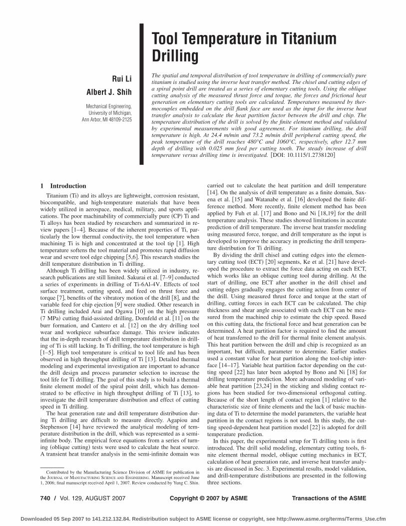
Experimental SetupThe Ti drilling experiment was conducted in a Mori Seiki TV

0 computer numerical control vertical machining center. Figure 1hows the experimental setup with the stationary drill and the Tiorkpiece driven by a spindle. The drill was stationary so four

hermocouples embedded on the flank face could be routedhrough coolant holes in the drill body to a data acquisition systemuring drilling �14�. The drill and machine spindle axes wereligned by a test indicator installed in the spindle. The location ofhe drill was adjusted in the horizontal plane until the eccentricityas less than 10 �m. The tilt of the drill was adjusted so that twolanes, which were 5 cm apart in height, both had less than0 �m eccentricity. Under the drill holder was a Kistler 9272ynamometer to measure the thrust force and torque.

The workpiece was a 38 mm diam grade two CP Ti bar. Therill was a 9.92 mm diam spiral point drill, Kennametal285A03906, with a S-shaped chisel edge. Compared to a con-entional twist drill, the chisel edge of the spiral point drill hadower negative rake angle. Therefore, the web could participate inutting, not just indenting like the conventional twist drill. Thiseduces the thrust force and makes the drill self-centering �25�.he tool material was WC in a 9.5 wt % Co matrix �Kennametal

ig. 1 Experimental setup with workpiece in the spindle andrill in a vertical tool holder

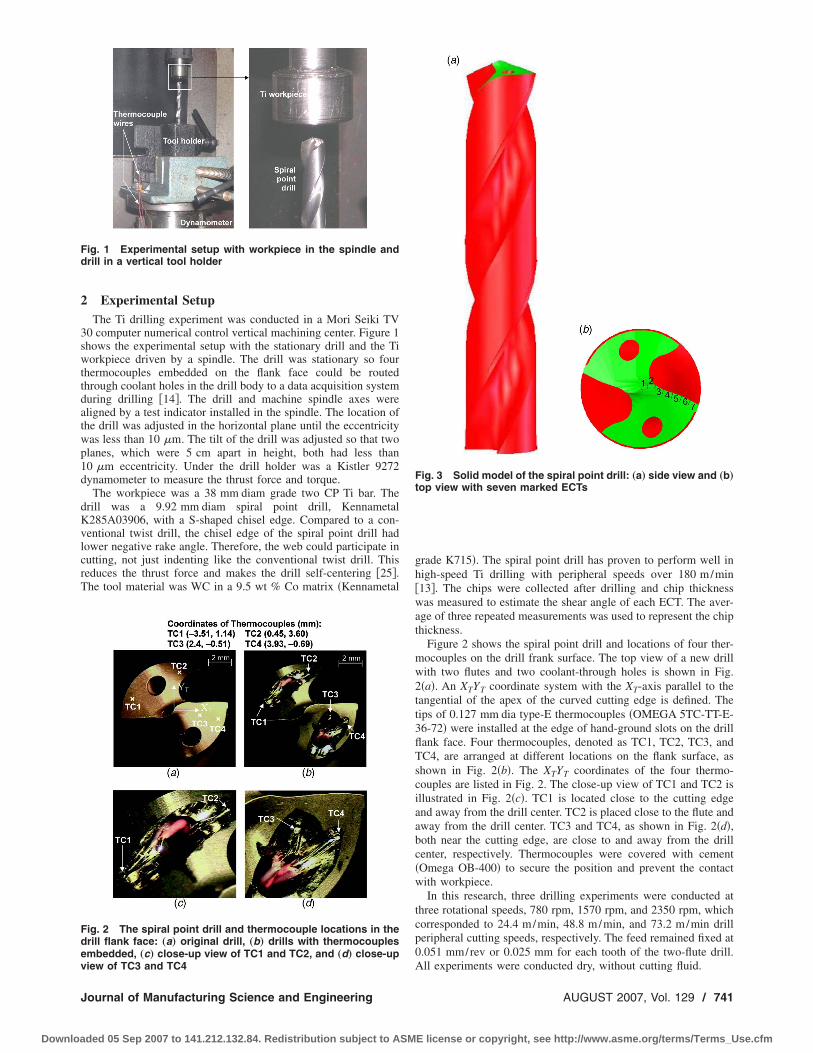
ig. 2 The spiral point drill and thermocouple locations in therill flank face: „a… original drill, „b… drills with thermocouplesmbedded, „c… close-up view of TC1 and TC2, and „d… close-up
iew of TC3 and TC4
ournal of Manufacturing Science and Engineering


grade K715�. The spiral point drill has proven to perform well inhigh-speed Ti drilling with peripheral speeds over 180 m/min�13�. The chips were collected after drilling and chip thicknesswas measured to estimate the shear angle of each ECT. The aver-age of three repeated measurements was used to represent the chipthickness.

Figure 2 shows the spiral point drill and locations of four ther-mocouples on the drill frank surface. The top view of a new drillwith two flutes and two coolant-through holes is shown in Fig.2�a�. An XTYT coordinate system with the XT-axis parallel to thetangential of the apex of the curved cutting edge is defined. Thetips of 0.127 mm dia type-E thermocouples �OMEGA 5TC-TT-E-36-72� were installed at the edge of hand-ground slots on the drillflank face. Four thermocouples, denoted as TC1, TC2, TC3, andTC4, are arranged at different locations on the flank surface, asshown in Fig. 2�b�. The XTYT coordinates of the four thermo-couples are listed in Fig. 2. The close-up view of TC1 and TC2 isillustrated in Fig. 2�c�. TC1 is located close to the cutting edgeand away from the drill center. TC2 is placed close to the flute andaway from the drill center. TC3 and TC4, as shown in Fig. 2�d�,both near the cutting edge, are close to and away from the drillcenter, respectively. Thermocouples were covered with cement�Omega OB-400� to secure the position and prevent the contactwith workpiece.

In this research, three drilling experiments were conducted atthree rotational speeds, 780 rpm, 1570 rpm, and 2350 rpm, whichcorresponded to 24.4 m/min, 48.8 m/min, and 73.2 m/min drillperipheral cutting speeds, respectively. The feed remained fixed at0.051 mm/rev or 0.025 mm for each tooth of the two-flute drill.

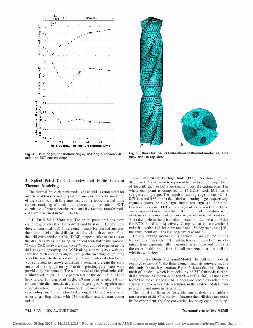
Fig. 3 Solid model of the spiral point drill: „a… side view and „b…top view with seven marked ECTs

All experiments were conducted dry, without cutting fluid.

AUGUST 2007, Vol. 129 / 741


3T

ioece

cttttTdswwmpihcaeur

Fa

7

Downloa

Spiral Point Drill Geometry and Finite Elementhermal ModelingThe thermal finite element model of the drill is established for

nverse heat transfer and temperature analysis. The solid modelingf the spiral point drill, elementary cutting tools, thermal finitelement modeling of the drill, oblique cutting mechanics in ECT,alculation of heat generation rate, and inverse heat transfer mod-ling are discussed in Sec. 3.1–3.6.

3.1 Drill Solid Modeling. The spiral point drill has moreomplex geometry than the conventional twist drill. To develop ahree-dimensional �3D� finite element mesh for thermal analysis,he solid model of the drill was established in three steps. First,he drill cross-section profile �DCSP� perpendicular to the axis ofhe drill was measured using an optical tool-maker microscope.hen, a CAD software, SOLIDWORKS™, was applied to generate therill body by sweeping the DCSP along a spiral curve with thepecified pitch and helix angle. Finally, the trajectory of grindingheel to generate the spiral drill point with S-shaped chisel edgeas simulated to remove unwanted material and create the solidodel of drill tip geometry. The drill grinding parameters were

rovided by Kennametal. The solid model of the spiral point drills illustrated in Fig. 3. Key parameters of the drill are a 30 degelix angle, 135 deg point angle, 1.9 mm point length, 1.4 mmoolant hole diameter, 52 deg chisel edge angle, 7 deg clearancengle at cutting corner, 0.43 mm width of margin, 1.4 mm chiseldge radius, and 1.8 mm chisel edge length. The drill was groundsing a grinding wheel with 150 mm diam and 1.1 mm corner

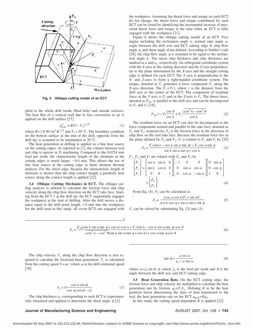
ig. 4 Rake angle, inclination angle, and angle between drillxis and ECT cutting edge

adius.

42 / Vol. 129, AUGUST 2007


3.2 Elementary Cutting Tools (ECT). As shown in Fig.3�b�, two ECTs are used to represent half of the chisel edge �webof the drill� and five ECTs are used to model the cutting edge. Thewhole drill point is composed of 14 ECTs. Each ECT has astraight cutting edge. The length of cutting edge of the ECT is0.71 mm and 0.85 mm in the chisel and cutting edge, respectively.Figure 4 shows the rake angle, inclination angle, and angle be-tween drill axis and ECT cutting edge of the seven ECTs. Theseangles were obtained from the drill solid model since there is noexisting formula to calculate these angles of the spiral point drill.The rake angle in the chisel edge is equal to −29 deg and −9 degfor ECTs 1 and 2, respectively. Compared to the conventionaltwist drill with a 118 deg point angle and −59 deg rake angle �26�,the spiral point drill has less negative rake angles.

Oblique cutting mechanics is applied to analyze the cuttingforces �18,26� in each ECT. Cutting forces in each ECT are ob-tained from experimentally measured thrust force and torque atthe onset of drilling, before the full engagement of the drill tipwith the workpiece.

3.3 Finite Element Thermal Model. The drill solid model isexported to ABAQUS™, the finite element analysis software used inthis study, for mesh generation. Figure 5 shows the finite elementmesh of the drill, which is modeled by 68,757 four-node tetrahe-dral elements. As shown in the top view in Fig. 5�b�, 13 nodes arelocated on the chisel edge and 11 nodes are placed on each cuttingedge to achieve reasonable resolution in the analysis of drill tem-perature distribution in Ti drilling.

The initial condition of finite element analysis is a uniformtemperature of 20°C in the drill. Because the drill does not rotate

Fig. 5 Mesh for the 3D finite element thermal model: „a… sideview and „b… top view

in the experiment, the free convection boundary condition is ap-

Transactions of the ASME


pTa

wod

oafclaes

tvittf

qf�

t

J

Downloa

lied to the whole drill inside �fluid hole� and outside surfaces.he heat flux of a vertical wall due to free convection in air ispplied on the drill surface �27�

qconv� = B�T − T��1.25 �1�

here B=1.8 W/m2 K1.25 and T�=20°C. The boundary conditionn the bottom surface at the end of the drill, opposite from therill tip, is assumed to be maintained at 20°C.

The heat generation in drilling is applied as a line heat sourcen the cutting edges. As reported in �1�, the contact between toolnd chip is narrow in Ti machining. Compared to the 0.0254 mmeed per tooth, the characteristic length of the elements at theutting edges is much larger, �0.4 mm. This allows the use ofine heat source at the cutting edge in finite element thermalnalysis. For the chisel edge, because the characteristic length oflements is shorter than the chip contact length, a parabolic heatource along the contact length is applied �22�.

3.4 Oblique Cutting Mechanics in ECT. The oblique cut-ing analysis is utilized to calculate the friction force and chipelocity along the chip flow direction on the ECT rake face. Start-ng from the ECT 1 at the drill tip, the ECT sequentially engageshe workpiece at the start of drilling. After the drill moves a dis-ance equal to the drill point length, 1.9 mm into the workpieceor the drill used in this study, all seven ECTs are engaged with

Fig. 6 Oblique cutting model of an ECT

ally measured and applied to determine the shear angle � �5�



the workpiece. Assuming the thrust force and torque on each ECTdo not change, the thrust force and torque contributed by eachECT can be found by identifying the incremental increase of mea-sured thrust force and torque at the time when an ECT is fullyengaged with the workpiece �21�.

Figure 6 shows the oblique cutting model of an ECT. Fiveangles including the inclination angle �, normal rake angle �,angle between the drill axis and ECT cutting edge �, chip flowangle �, and shear angle � are defined. According to Stabler’s rule�28�, the chip flow angle � is assumed to be equal to the inclina-tion angle �. The uncut chip thickness and chip thickness aremarked as a and ac, respectively. An orthogonal coordinate systemwith the X-axis in the cutting direction and the Z-axis perpendicu-lar to the plane determined by the X-axis and the straight cuttingedge is defined for each ECT. The Y-axis is perpendicular to theX- and Z-axes to form a right-handed coordinate system. Thetorque, denoted as T, generates a force component Fc along theX-axis direction. The Fc=T /r, where r is the distance from thedrill axis to the center of the ECT. The component of resultantforce in the Y-axis is Fl and in the Z-axis is Ft. The thrust force,denoted as FTh, is parallel to the drill axis and can be decomposedto Ft and Fl �18�,

FTh = − Fl

cos �

cos �+ Ft

�cos2 � − cos2 �

cos ��2�

The resultant force on an ECT can also be decomposed to theforce components normal and parallel to the rake face, denoted asFn and Ff, respectively. Ff is the friction force in the direction ofchip flow on the tool rake face. Because the resultant force lies inthe plane defined by Fn and Ff, Fl is related to Fc and Ft by �29�

Fl =Fc�sin � − cos � sin � tan �� − Ft cos � tan �

sin � sin � tan � + cos ��3�

Fc, Fl, and Ft are related with Fn and Ff by

�Fl

Fc

Ft� = cos � sin � 0

sin � cos � 0

0 0 1− 1 0 0

0 sin � cos �

0 cos � − sin �0 sin �

0 cos �

1 0

��Fn

Ff� �4�

From Eq. �4�, Ff can be calculated as

Ff =�cos � cos ��Ft + sin �Fc

cos � cos � + sin � sin � sin ��5�

F can be solved by substituting Eq. �2� into �3�.
t
Ft =FTh�sin � sin � tan � + cos �� cos � + Fc�sin � − cos � sin � tan �� cos �

�cos2 � − cos2 ��sin � sin � tan � + cos �� + cos � tan � cos ��6�

The chip velocity Vc along the chip flow direction is also re-uired to calculate the frictional heat generation. Vc is calculatedrom the cutting speed V=r, where is the drill rotational speed30�

Vc = Vcos � sin �

cos � cos�� − ��7�

The chip thickness ac corresponding to each ECT is experimen-

tan � =a cos �

ac − a sin ��8�

where a= fd sin �, in which fd is the feed per tooth and � is theangle between the drill axis and ECT cutting edge.

3.5 Heat Generation Rate. On the ECT cutting edge, thefriction force and chip velocity are multiplied to calculate the heatgeneration rate by friction, qf =FfVc. Defining K to be the heatpartition factor determining the ratio of heat transferred to thetool, the heat generation rate on the ECT qtool=Kqf.

In this study, the cutting speed dependent K is applied �22�

AUGUST 2007, Vol. 129 / 743


wTlpF

t

wtct

u

7

Downloa

K = 1 − 1 + 0.45kt

kw

�dw

Vcl�−1

�9�

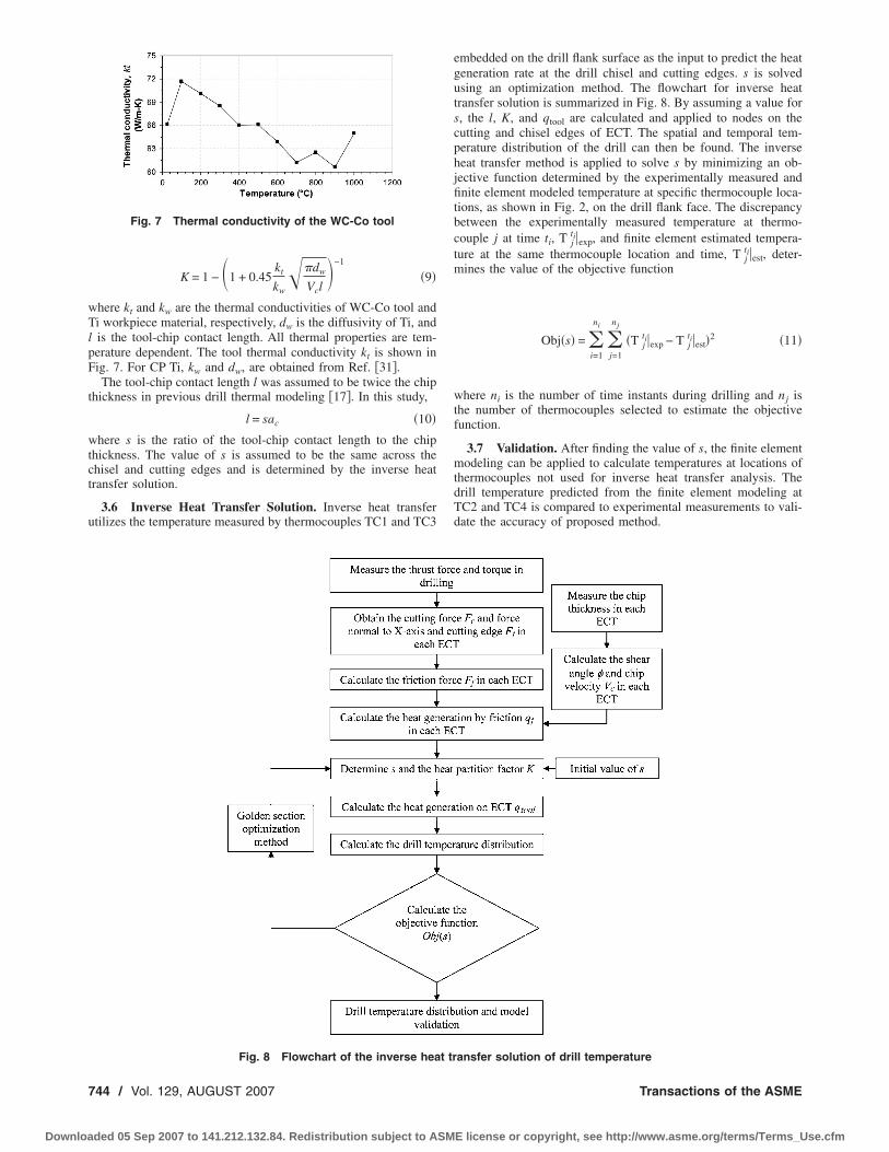
here kt and kw are the thermal conductivities of WC-Co tool andi workpiece material, respectively, dw is the diffusivity of Ti, andis the tool-chip contact length. All thermal properties are tem-erature dependent. The tool thermal conductivity kt is shown inig. 7. For CP Ti, kw and dw, are obtained from Ref. �31�.The tool-chip contact length l was assumed to be twice the chip

hickness in previous drill thermal modeling �17�. In this study,

l = sac �10�

here s is the ratio of the tool-chip contact length to the chiphickness. The value of s is assumed to be the same across thehisel and cutting edges and is determined by the inverse heatransfer solution.

3.6 Inverse Heat Transfer Solution. Inverse heat transfertilizes the temperature measured by thermocouples TC1 and TC3

Fig. 7 Thermal conductivity of the WC-Co tool

Fig. 8 Flowchart of the inverse heat tr

44 / Vol. 129, AUGUST 2007


embedded on the drill flank surface as the input to predict the heatgeneration rate at the drill chisel and cutting edges. s is solvedusing an optimization method. The flowchart for inverse heattransfer solution is summarized in Fig. 8. By assuming a value fors, the l, K, and qtool are calculated and applied to nodes on thecutting and chisel edges of ECT. The spatial and temporal tem-perature distribution of the drill can then be found. The inverseheat transfer method is applied to solve s by minimizing an ob-jective function determined by the experimentally measured andfinite element modeled temperature at specific thermocouple loca-tions, as shown in Fig. 2, on the drill flank face. The discrepancybetween the experimentally measured temperature at thermo-couple j at time ti, T j

ti�exp, and finite element estimated tempera-ture at the same thermocouple location and time, T j

ti�est, deter-mines the value of the objective function

Obj�s� = �i=1

ni

�j=1

nj

�T jti�exp − T j

ti�est�2 �11�

where ni is the number of time instants during drilling and nj isthe number of thermocouples selected to estimate the objectivefunction.

3.7 Validation. After finding the value of s, the finite elementmodeling can be applied to calculate temperatures at locations ofthermocouples not used for inverse heat transfer analysis. Thedrill temperature predicted from the finite element modeling atTC2 and TC4 is compared to experimental measurements to vali-date the accuracy of proposed method.

ansfer solution of drill temperature



4

tf

mhf7sbtpd

mttbcttc

sitesaeawcta

tfiumsatAteti

fEhctd

msmscm

p1e

J

Downloa

Experimental ResultsThe experimentally measured chip thickness, thrust force, and

orque are applied to calculate the shear angle, ECT cutting forces,rictional heat generation, and heat partition factor.

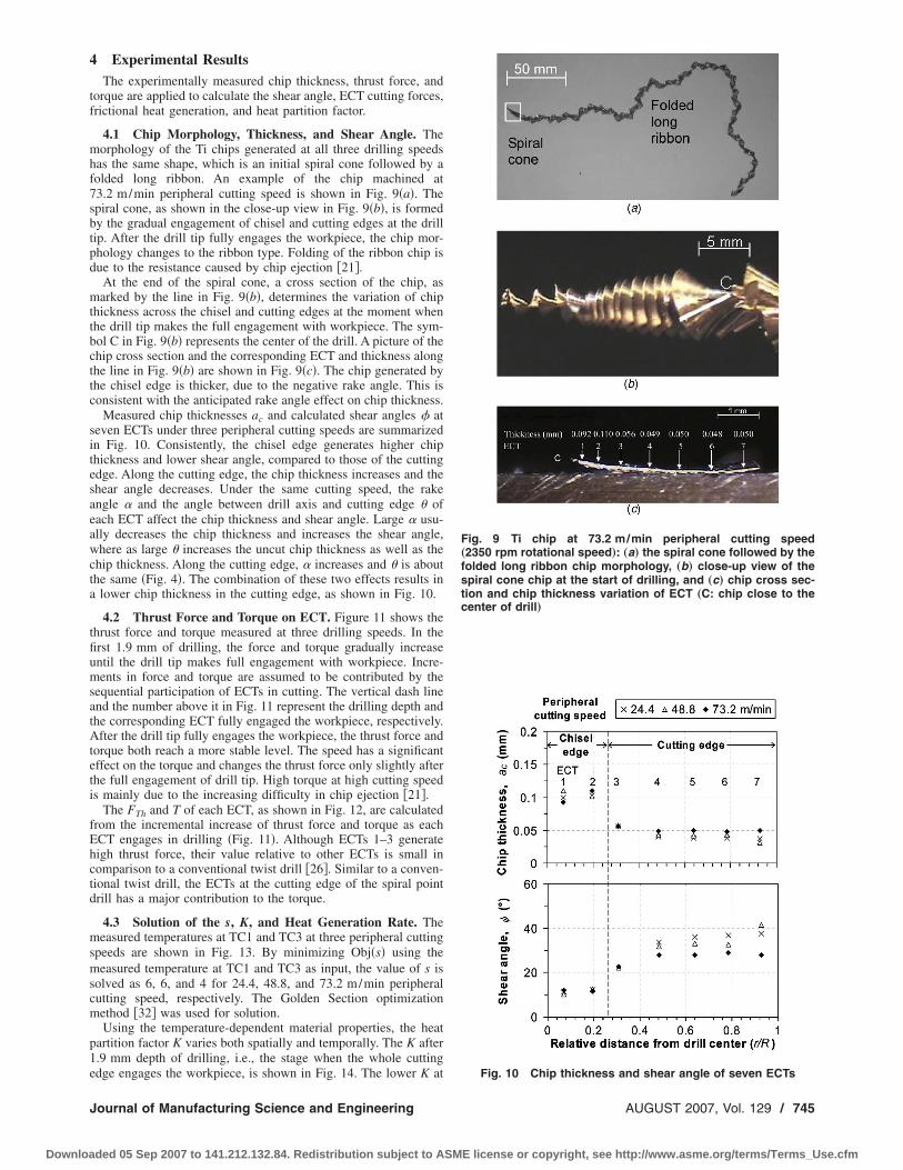
4.1 Chip Morphology, Thickness, and Shear Angle. Theorphology of the Ti chips generated at all three drilling speeds

as the same shape, which is an initial spiral cone followed by aolded long ribbon. An example of the chip machined at3.2 m/min peripheral cutting speed is shown in Fig. 9�a�. Thepiral cone, as shown in the close-up view in Fig. 9�b�, is formedy the gradual engagement of chisel and cutting edges at the drillip. After the drill tip fully engages the workpiece, the chip mor-hology changes to the ribbon type. Folding of the ribbon chip isue to the resistance caused by chip ejection �21�.

At the end of the spiral cone, a cross section of the chip, asarked by the line in Fig. 9�b�, determines the variation of chip

hickness across the chisel and cutting edges at the moment whenhe drill tip makes the full engagement with workpiece. The sym-ol C in Fig. 9�b� represents the center of the drill. A picture of thehip cross section and the corresponding ECT and thickness alonghe line in Fig. 9�b� are shown in Fig. 9�c�. The chip generated byhe chisel edge is thicker, due to the negative rake angle. This isonsistent with the anticipated rake angle effect on chip thickness.

Measured chip thicknesses ac and calculated shear angles � ateven ECTs under three peripheral cutting speeds are summarizedn Fig. 10. Consistently, the chisel edge generates higher chiphickness and lower shear angle, compared to those of the cuttingdge. Along the cutting edge, the chip thickness increases and thehear angle decreases. Under the same cutting speed, the rakengle � and the angle between drill axis and cutting edge � ofach ECT affect the chip thickness and shear angle. Large � usu-lly decreases the chip thickness and increases the shear angle,here as large � increases the uncut chip thickness as well as the

hip thickness. Along the cutting edge, � increases and � is abouthe same �Fig. 4�. The combination of these two effects results inlower chip thickness in the cutting edge, as shown in Fig. 10.

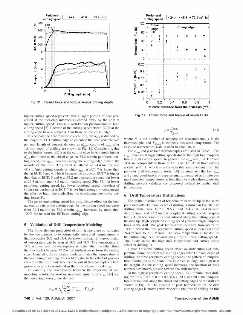
4.2 Thrust Force and Torque on ECT. Figure 11 shows thehrust force and torque measured at three drilling speeds. In therst 1.9 mm of drilling, the force and torque gradually increasentil the drill tip makes full engagement with workpiece. Incre-ents in force and torque are assumed to be contributed by the

equential participation of ECTs in cutting. The vertical dash linend the number above it in Fig. 11 represent the drilling depth andhe corresponding ECT fully engaged the workpiece, respectively.fter the drill tip fully engages the workpiece, the thrust force and

orque both reach a more stable level. The speed has a significantffect on the torque and changes the thrust force only slightly afterhe full engagement of drill tip. High torque at high cutting speeds mainly due to the increasing difficulty in chip ejection �21�.

The FTh and T of each ECT, as shown in Fig. 12, are calculatedrom the incremental increase of thrust force and torque as eachCT engages in drilling �Fig. 11�. Although ECTs 1–3 generateigh thrust force, their value relative to other ECTs is small inomparison to a conventional twist drill �26�. Similar to a conven-ional twist drill, the ECTs at the cutting edge of the spiral pointrill has a major contribution to the torque.

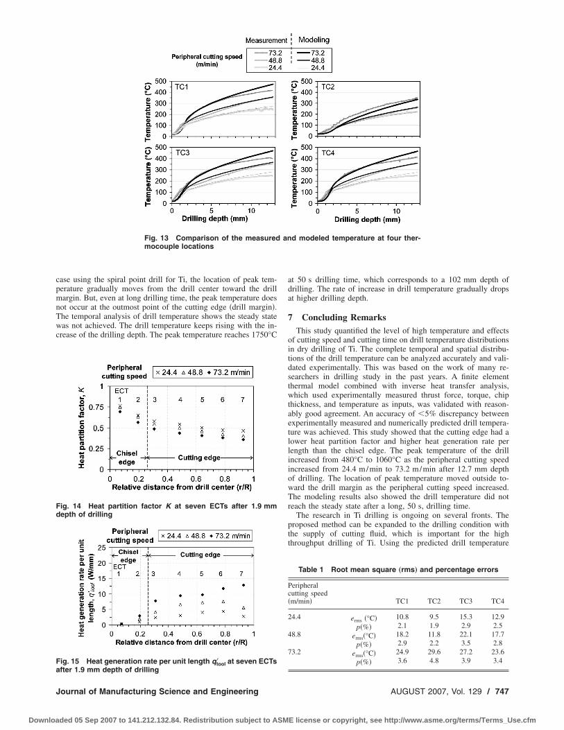
4.3 Solution of the s, K, and Heat Generation Rate. Theeasured temperatures at TC1 and TC3 at three peripheral cutting

peeds are shown in Fig. 13. By minimizing Obj�s� using theeasured temperature at TC1 and TC3 as input, the value of s is

olved as 6, 6, and 4 for 24.4, 48.8, and 73.2 m/min peripheralutting speed, respectively. The Golden Section optimizationethod �32� was used for solution.Using the temperature-dependent material properties, the heat

artition factor K varies both spatially and temporally. The K after.9 mm depth of drilling, i.e., the stage when the whole cutting
dge engages the workpiece, is shown in Fig. 14. The lower K at


Fig. 9 Ti chip at 73.2 m/min peripheral cutting speed„2350 rpm rotational speed…: „a… the spiral cone followed by thefolded long ribbon chip morphology, „b… close-up view of thespiral cone chip at the start of drilling, and „c… chip cross sec-tion and chip thickness variation of ECT „C: chip close to thecenter of drill…

Fig. 10 Chip thickness and shear angle of seven ECTs

AUGUST 2007, Vol. 129 / 745


hehcc

tp1tqto4ttapstt

gf1

5

btoTtetcg

mt

7

Downloa

igher cutting speed represents that a larger portion of heat gen-rated at the tool-chip interface is carried away by the chip atigher cutting speed. This is a well-known phenomenon at highutting speed �5�. Because of the cutting speed effect, ECTs at theutting edge have a higher K than those on the chisel edge.

To compare the heat transfer to each ECT, the qtool is divided byhe length of ECT cutting edge to calculate the heat generate rateer unit length of contact, denoted as qtool� . Results of qtool� after.9 mm depth of drilling are shown in Fig. 15. Consistently, dueo the higher torque, ECTs at the cutting edge have a much higher

tool� than those at the chisel edge. At 73.2 m/min peripheral cut-ing speed, the qtool� increases along the cutting edge toward theutside of the drill. This trend is altered at 24.4 m/min and8.8 m/min cutting speeds at which qtool� at ECT 7 is lower thanhat at ECTs 5 and 6. This is because the torque of ECT 7 is higherhan that of ECTs 5 and 6 at 73.2 m/min cutting speed but lowert 24.4 m/min and 48.8 m/min cutting speed �Fig. 12�. At lowereripheral cutting speed, i.e., lower rotational speed, the effect oftrain rate hardening at ECT 7 is not high enough to compensatehe effect of high rake angle �Fig. 4�, which generates lower cut-ing forces Fc.

The peripheral cutting speed has a significant effect on the heateneration rate at the cutting edge. As the cutting speed increasesrom 24.4 m/min to 73.2 m/min, qtool� increases by more than00% for most of the ECTs on cutting edge.

Validation of Drill Temperature ModelingThe finite element prediction of drill temperature is validated

y the comparison to experimentally measured temperatures athermocouples TC2 and TC4. As shown in Fig. 13, a good matchf temperature can be seen at TC2 and TC4. The temperature atC2 is lower and the discrepancy is higher than the other three

hermocouples because TC2 is the furthest away from the cuttingdge. Generally, the simulation underestimates the temperature athe beginning of drilling. This is likely due to the effect of groovesarved on the drill flank face used to install thermocouples. Theserooves were not considered in the finite element modeling.

To quantify the discrepancy between the experimental andodeling results, the root mean square �rms� error erms �33� and

he percentage error p are defined

e =1

N

�T ti − T ti �2 �12�

Fig. 11 Thrust force and torque versus drilling depth

rms �N�

i=1j�exp j�est

46 / Vol. 129, AUGUST 2007


p =erms

Tj�peak�13�

where N is the number of temperature measurements, j is thethermocouple, and Tj�peak is the peak measured temperature. Theabsolute temperature scale is used to calculate p.

The erms and p at four thermocouples are listed in Table 1. Theerms increases at high cutting speeds due to the high tool tempera-ture at high cutting speed. In general, the erms and p at TC2 andTC4 are comparable to those of TC1 and TC3. At all three cuttingspeeds, p�5%, which is a considerable improvement from theprevious drill temperature study �18�. In summary, the low ermsand p and good match of experimentally measured and finite ele-ment modeled temperatures at four thermocouples throughout thedrilling process validates the proposed method to predict drilltemperature.

6 Drill Temperature DistributionsThe spatial distribution of temperature near the tip of the spiral

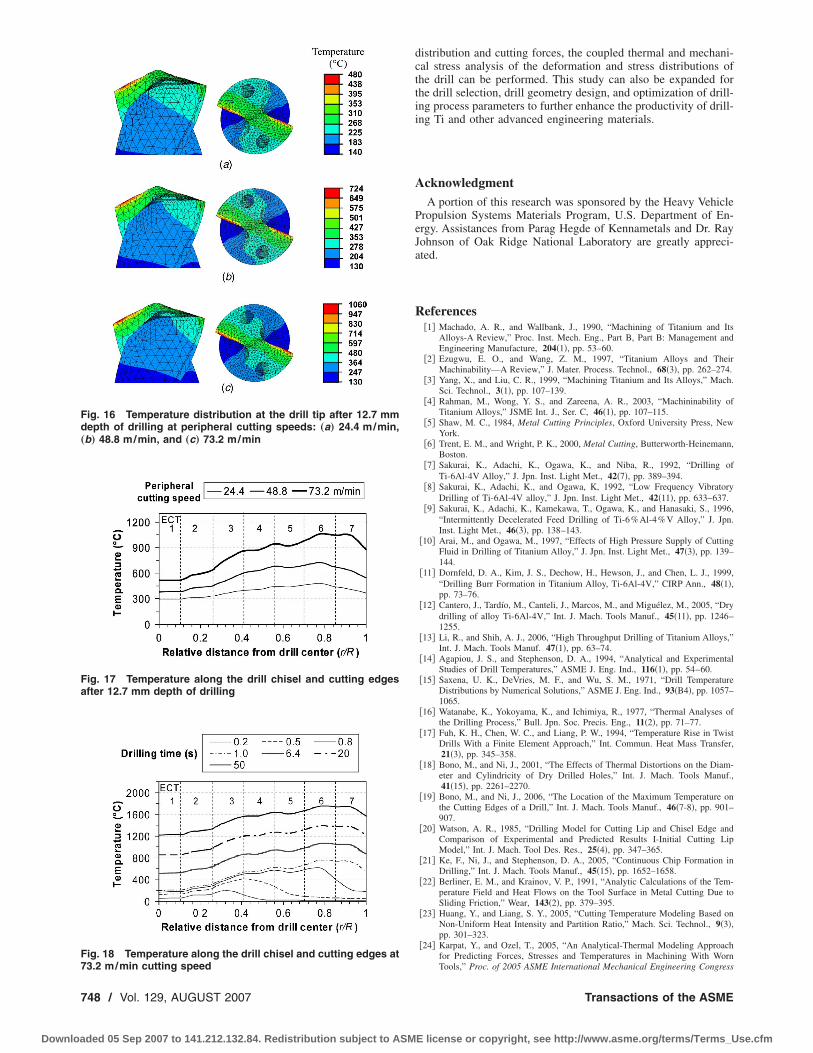
point drill after 12.7 mm depth of drilling is shown in Fig. 16. Thedrilling time was 19.2 s, 9.6 s, and 6.4 s at 24.4 m/min,48.8 m/min, and 73.2 m/min peripheral cutting speeds, respec-tively. High temperature is concentrated along the cutting edge atthe drill tip. High peripheral cutting speed generates high tempera-tures in the drill. The peak temperature increases from 480°C to1060°C when the drill peripheral cutting speed is increased from24.4 m/min to 73.2 m/min. The peak temperature is located onthe cutting edge near the drill margin for all three cutting speeds.This study shows the high drill temperature and cutting speedeffect in drilling Ti.

Figure 17 shows cutting speed effect on distributions of tem-perature along the chisel and cutting edges after 12.7 mm depth ofdrilling. At three peripheral cutting speeds, the pattern of tempera-ture distribution is the same: low at the chisel edge and high nearthe margin. As the cutting speed increases, the location of peaktemperature moves outside toward the drill margin.

At the highest peripheral cutting speed, 73.2 m/min, after drill-ing for 0.2 s, 0.5 s, 0.8 s, 1.0 s, 6.4 s, 20 s, and 50 s, the tempera-ture distributions along the chisel and cutting edges of the drill areshown in Fig. 18. The location of peak temperature on the drill

Fig. 12 Thrust force and torque of seven ECTs

cutting edges is moving with respect to the time of drilling. In this



cpmnTwc

Fd

Fa

J

Downloa

ase using the spiral point drill for Ti, the location of peak tem-erature gradually moves from the drill center toward the drillargin. But, even at long drilling time, the peak temperature does

ot occur at the outmost point of the cutting edge �drill margin�.he temporal analysis of drill temperature shows the steady stateas not achieved. The drill temperature keeps rising with the in-

rease of the drilling depth. The peak temperature reaches 1750°C

Fig. 13 Comparison of the measuredmocouple locations

ig. 14 Heat partition factor K at seven ECTs after 1.9 mmepth of drilling

ig. 15 Heat generation rate per unit length qtool� at seven ECTs
fter 1.9 mm depth of drilling


at 50 s drilling time, which corresponds to a 102 mm depth ofdrilling. The rate of increase in drill temperature gradually dropsat higher drilling depth.

7 Concluding RemarksThis study quantified the level of high temperature and effects

of cutting speed and cutting time on drill temperature distributionsin dry drilling of Ti. The complete temporal and spatial distribu-tions of the drill temperature can be analyzed accurately and vali-dated experimentally. This was based on the work of many re-searchers in drilling study in the past years. A finite elementthermal model combined with inverse heat transfer analysis,which used experimentally measured thrust force, torque, chipthickness, and temperature as inputs, was validated with reason-ably good agreement. An accuracy of �5% discrepancy betweenexperimentally measured and numerically predicted drill tempera-ture was achieved. This study showed that the cutting edge had alower heat partition factor and higher heat generation rate perlength than the chisel edge. The peak temperature of the drillincreased from 480°C to 1060°C as the peripheral cutting speedincreased from 24.4 m/min to 73.2 m/min after 12.7 mm depthof drilling. The location of peak temperature moved outside to-ward the drill margin as the peripheral cutting speed increased.The modeling results also showed the drill temperature did notreach the steady state after a long, 50 s, drilling time.

The research in Ti drilling is ongoing on several fronts. Theproposed method can be expanded to the drilling condition withthe supply of cutting fluid, which is important for the highthroughput drilling of Ti. Using the predicted drill temperature

Table 1 Root mean square „rms… and percentage errors

Peripheralcutting speed�m/min� TC1 TC2 TC3 TC4

24.4 erms �°C� 10.8 9.5 15.3 12.9p�%� 2.1 1.9 2.9 2.5

48.8 erms�°C� 18.2 11.8 22.1 17.7p�%� 2.9 2.2 3.5 2.8

73.2 erms�°C� 24.9 29.6 27.2 23.6p�%� 3.6 4.8 3.9 3.4

d modeled temperature at four ther-
an
AUGUST 2007, Vol. 129 / 747


Fd„

Fa

F73.2 m/min cutting speed

748 / Vol. 129, AUGUST 2007

Downloaded 05 Sep 2007 to 141.212.132.84. Redistribution subject to ASM

distribution and cutting forces, the coupled thermal and mechani-cal stress analysis of the deformation and stress distributions ofthe drill can be performed. This study can also be expanded forthe drill selection, drill geometry design, and optimization of drill-ing process parameters to further enhance the productivity of drill-ing Ti and other advanced engineering materials.

AcknowledgmentA portion of this research was sponsored by the Heavy Vehicle

Propulsion Systems Materials Program, U.S. Department of En-ergy. Assistances from Parag Hegde of Kennametals and Dr. RayJohnson of Oak Ridge National Laboratory are greatly appreci-ated.

References�1� Machado, A. R., and Wallbank, J., 1990, “Machining of Titanium and Its

Alloys-A Review,” Proc. Inst. Mech. Eng., Part B, Part B: Management andEngineering Manufacture, 204�1�, pp. 53–60.

�2� Ezugwu, E. O., and Wang, Z. M., 1997, “Titanium Alloys and TheirMachinability—A Review,” J. Mater. Process. Technol., 68�3�, pp. 262–274.

�3� Yang, X., and Liu, C. R., 1999, “Machining Titanium and Its Alloys,” Mach.Sci. Technol., 3�1�, pp. 107–139.

�4� Rahman, M., Wong, Y. S., and Zareena, A. R., 2003, “Machininability ofTitanium Alloys,” JSME Int. J., Ser. C, 46�1�, pp. 107–115.

�5� Shaw, M. C., 1984, Metal Cutting Principles, Oxford University Press, NewYork.

�6� Trent, E. M., and Wright, P. K., 2000, Metal Cutting, Butterworth-Heinemann,Boston.

�7� Sakurai, K., Adachi, K., Ogawa, K., and Niba, R., 1992, “Drilling ofTi-6Al-4V Alloy,” J. Jpn. Inst. Light Met., 42�7�, pp. 389–394.

�8� Sakurai, K., Adachi, K., and Ogawa, K, 1992, “Low Frequency VibratoryDrilling of Ti-6Al-4V alloy,” J. Jpn. Inst. Light Met., 42�11�, pp. 633–637.

�9� Sakurai, K., Adachi, K., Kamekawa, T., Ogawa, K., and Hanasaki, S., 1996,“Intermittently Decelerated Feed Drilling of Ti-6%Al-4%V Alloy,” J. Jpn.Inst. Light Met., 46�3�, pp. 138–143.

�10� Arai, M., and Ogawa, M., 1997, “Effects of High Pressure Supply of CuttingFluid in Drilling of Titanium Alloy,” J. Jpn. Inst. Light Met., 47�3�, pp. 139–144.

�11� Dornfeld, D. A., Kim, J. S., Dechow, H., Hewson, J., and Chen, L. J., 1999,“Drilling Burr Formation in Titanium Alloy, Ti-6Al-4V,” CIRP Ann., 48�1�,pp. 73–76.

�12� Cantero, J., Tardío, M., Canteli, J., Marcos, M., and Miguélez, M., 2005, “Drydrilling of alloy Ti-6Al-4V,” Int. J. Mach. Tools Manuf., 45�11�, pp. 1246–1255.

�13� Li, R., and Shih, A. J., 2006, “High Throughput Drilling of Titanium Alloys,”Int. J. Mach. Tools Manuf. 47�1�, pp. 63–74.

�14� Agapiou, J. S., and Stephenson, D. A., 1994, “Analytical and ExperimentalStudies of Drill Temperatures,” ASME J. Eng. Ind., 116�1�, pp. 54–60.

�15� Saxena, U. K., DeVries, M. F., and Wu, S. M., 1971, “Drill TemperatureDistributions by Numerical Solutions,” ASME J. Eng. Ind., 93�B4�, pp. 1057–1065.

�16� Watanabe, K., Yokoyama, K., and Ichimiya, R., 1977, “Thermal Analyses ofthe Drilling Process,” Bull. Jpn. Soc. Precis. Eng., 11�2�, pp. 71–77.

�17� Fuh, K. H., Chen, W. C., and Liang, P. W., 1994, “Temperature Rise in TwistDrills With a Finite Element Approach,” Int. Commun. Heat Mass Transfer,21�3�, pp. 345–358.

�18� Bono, M., and Ni, J., 2001, “The Effects of Thermal Distortions on the Diam-eter and Cylindricity of Dry Drilled Holes,” Int. J. Mach. Tools Manuf.,41�15�, pp. 2261–2270.

�19� Bono, M., and Ni, J., 2006, “The Location of the Maximum Temperature onthe Cutting Edges of a Drill,” Int. J. Mach. Tools Manuf., 46�7-8�, pp. 901–907.

�20� Watson, A. R., 1985, “Drilling Model for Cutting Lip and Chisel Edge andComparison of Experimental and Predicted Results I-Initial Cutting LipModel,” Int. J. Mach. Tool Des. Res., 25�4�, pp. 347–365.

�21� Ke, F., Ni, J., and Stephenson, D. A., 2005, “Continuous Chip Formation inDrilling,” Int. J. Mach. Tools Manuf., 45�15�, pp. 1652–1658.

�22� Berliner, E. M., and Krainov, V. P., 1991, “Analytic Calculations of the Tem-perature Field and Heat Flows on the Tool Surface in Metal Cutting Due toSliding Friction,” Wear, 143�2�, pp. 379–395.

�23� Huang, Y., and Liang, S. Y., 2005, “Cutting Temperature Modeling Based onNon-Uniform Heat Intensity and Partition Ratio,” Mach. Sci. Technol., 9�3�,pp. 301–323.

�24� Karpat, Y., and Ozel, T., 2005, “An Analytical-Thermal Modeling Approachfor Predicting Forces, Stresses and Temperatures in Machining With Worn

ig. 16 Temperature distribution at the drill tip after 12.7 mmepth of drilling at peripheral cutting speeds: „a… 24.4 m/min,b… 48.8 m/min, and „c… 73.2 m/min

ig. 17 Temperature along the drill chisel and cutting edgesfter 12.7 mm depth of drilling

ig. 18 Temperature along the drill chisel and cutting edges at
Tools,” Proc. of 2005 ASME International Mechanical Engineering Congress


J

Downloa

and Exposition, ASME New York, Vol. 16, pp. 489–498.�25� Ernst, H., and Haggerty, W. A., 1958, “Spiral Point Drill—New Concept in

Drill Point Geometry,” Trans. ASME, 80, pp. 1059–1072.�26� Strenkowski, J. S., Hsieh, C. C., and Shih, A. J. 2004, “An Analytical Finite

Element Technique for Predicting Thrust Force and Torque in Drilling,” Int. J.Mach. Tools Manuf., 44�12-13�, pp. 1413–1421.

�27� Orfueil, M., 1987, Electric Process Heating, Battelle Press, Columbus, OH.�28� Stabler, G., 1951, “The Fundamental Geometry of Cutting Tools,” Proc. Inst.

Mech. Eng., 165�63�, pp. 14–21.�29� Lin, G. C., Mathew, P., Oxley, P. L. B., and Watson, A. R., 1982, “Predicting



Cutting Forces for Oblique Machining Conditions,” Proc. Inst. Mech. Eng.,196, pp. 141–148.

�30� Shaw, M. C., Cook, N. H., and Smith, P. A., 1952, “Mechanics of Three-Dimensional Cutting Operations,” Trans. ASME, 74�6�, pp. 1055–1064.

�31� ASM, 1994, Material Properties Handbook: Titanium Alloys, ASM Interna-tional, Materials Park, OH.

�32� Himmelblau, D. M., 1972, Applied Nonlinear Programming, McGraw-Hill,New York.

�33� Luo, J., and Shih, A. J., 2005, “Inverse Heat Transfer of the Heat Flux due toInduction Heating,” ASME J. Manuf. Sci. Tech. 127, pp. 555–563.

AUGUST 2007, Vol. 129 / 749


Documents

Tool Temperature in Titanium Drilling - University of …career.engin.umich.edu/.../08/07_ASMELitool_temp_in_Ti_drilling.pdf · Rui Li Albert J. Shih MechanicalEngineering, UniversityofMichigan,