National Poverty Center Working Paper Series

#16-06

August 2016

Growing Wealth Gaps in Education

Fabian Pfeffer, University of Michigan

This paper is available online at the National Poverty Center Working Paper Series index at: http://www.npc.umich.edu/publications/working_papers/

Any opinions, findings, conclusions, or recommendations expressed in this material are those of the author(s) and do

not necessarily reflect the view of the National Poverty Center or any sponsoring agency.

Growing Wealth Gaps in Education

Fabian T. Pfeffer∗

University of Michigan

Abstract

Prior research on trends in educational inequality has focused chiefly on changing

gaps in educational attainment by family income or parental occupation. In contrast,

this contribution provides the first assessment of trends in educational attainment by

family wealth and suggests that we should be at least as much concerned about growing

wealth gaps in education. Despite overall growth in educational attainment and some

signs of decreasing wealth gaps in high school attainment and college access, I find a

large and rapidly increasing wealth gap in college attainment between cohorts born in

the 1970 and 1980s, respectively. This growing wealth gap in higher educational at-

tainment co-occurred with a rise in inequality in children’s wealth backgrounds, though

the analyses also suggest that the latter does not fully account for the former. Never-

theless, the results reported here raise concerns about the distribution of educational

opportunity among today’s children who grow up in a context of particularly extreme

wealth inequality.

∗I gratefully acknowledge funding for this project from the Spencer Foundation (grant #201300139) aswell as very helpful comments from Sheldon Danziger, Thomas DiPrete, Alexandra Killewald, and RobertSchoeni. Earlier versions of this paper were presented at meetings of the Population Association of America,the American Sociological Association, and the Research Committee on Social Inequality and Mobility(RC28). The collection of data used in this study was partly supported by the National Institutes ofHealth (grant #R01HD069609) and the National Science Foundation (grant #1157698). Please direct allcorrespondence to Fabian T. Pfeffer, University of Michigan, 426 Thompson Street, 3240 Institute for SocialResearch, Ann Arbor, Michigan 48104, fpfeffer@umich.edu.

Introduction

Family wealth – measured as the net value of all financial and real assets a family owns

– is much more unequally distributed than other indicators of families’ economic wellbeing

(Keister and Moller 2000). Research has documented that this already large inequality in

family wealth in the United States has been increasing substantially over the last decades

(Wolff 1995; Keister 2000; Piketty 2014; Saez and Zucman 2014) and particularly strongly

since the Great Recession (Pfeffer et al. 2013; Wolff 2016). One concern about growing wealth

inequality is that it may also increase the rigidity of U.S. society, in particular by contributing

to inequalities in educational opportunity. In fact, a growing body of research suggests that

parental wealth plays an important role in the educational attainment of children in the

United States and elsewhere (Conley 2001; Morgan and Kim 2006; Belley and Lochner 2007;

Pfeffer 2011). However, to date, there is no empirical evidence on whether and to what

extent wealth gaps in education have grown. This contribution provides the first empirical

assessment of trends in wealth inequality in educational outcomes based on newly available

data from the Panel Study of Income Dynamics (PSID). It also documents the extent to

which these changes in wealth gaps in education can be accounted for solely by changes in

the distribution of family wealth. Together, these analyses thus also speak to concerns about

the potential long-term implications of the most recent and sharp increase in family wealth

inequality in terms of the future distribution of educational outcomes.

I begin by reviewing prior research on cohort trends in educational inequality. In the next

section, I argue that this prior evidence, which is restricted to other socio-economic indicators

of family background, does not allow inferences about trends in wealth gaps: Family wealth

is empirically and conceptually distinct from more commonly used socio-economic indicators

and it contributes unique predictive power to assessments of children’s educational outcomes.

After describing the data, measures, and methods, I estimate the association between family

wealth and children’s educational attainment, unconditional and conditional on other socio-

1

economic characteristics of families, and document how wealth-education associations have

changed over recent cohorts. Finally, I decompose these changes into those that can be

accounted for by changes in wealth inequality, an exercise that gains particular importance

at the backdrop of an assessment of the level of wealth inequality among today’s children.

Background and Motivation

Prior research on trends in educational inequality

The study of cohort trends in socio-economic inequality in education has been an active

area of empirical investigation for several decades (e.g. Treiman 1970; Mare 1981; Shavit

and Blossfeld 1993; Harding et al. 2004). Research in this area investigates the changing

relationship between educational attainment and a variety of indicators of socio-economic

background. One set of contributions draws on occupation-based measures of parents’ social

class and documents remarkably stable class gaps in children’s educational outcomes in the

U.S. over much of the 20th and early 21st century (Hout et al. 1993; Roksa et al. 2007; Pfeffer

and Hertel 2015). Other research tracks the association between children’s and their parents’

highest educational status and also finds largely stable levels of educational inequality tied

to parental education (Mare 1981; Hout and Dohan 1996; Pfeffer 2008; Hout and Janus

2011; Bloome and Western 2011) as well as some signs of growing gaps for more recent

cohorts (Buchmann and DiPrete 2006; Hertz et al. 2007; Roksa et al. 2007; Pfeffer and

Hertel 2015). The most notable and widely discussed changes in educational inequality,

however, have been found in relation to family income: Reardon (2011) documents that the

gaps in educational achievement (i.e. test scores) between children from high-income and

low-income families has been growing steadily for at least fifty years. Similarly, income gaps

in higher education have also grown: Belley and Lochner (2007) observe substantial increases

in income inequality in college attendance, comparing a cohort born in the early 1960s to a

cohort born in the early 1980s. Bailey and Dynarski (2011) show that these trends extend to

2

growing income gaps in college graduation among the same cohorts. While income gaps in

college attendance have held stable for more recent cohorts (Chetty et al. 2014; Ziol-Guest

and Lee 2016), income gaps in college attainment have continued to increase (Duncan and

Kalil 2015; Ziol-Guest and Lee 2016). The most recent estimates indicate that the difference

in college graduation between children from the bottom and the top family income quintile

approaches 50 percentage points (Ziol-Guest and Lee 2016).

Overall, then, cohort changes in the distribution of educational attainment are more

pronounced in relation to parental income than in relation to parental education or parental

occupations. It may thus be tempting to infer that rising income gaps in education should

also manifest in rising gaps related to family wealth; after all both are monetary dimensions

of families’ socio-economic standing. However, as I will argue next, such direct inference is

neither empirically nor conceptually valid – wealth is distinct from income, its association

with education is distinct, and trends in that association may thus be distinct, too.

Wealth as an independent predictor of educational attainment

Some see conceptually few differences between wealth and income. In a strict model of

neoclassical economics – that is, a world with perfect credit markets and in which wealth

is accumulated from income rather than intergenerational transfers – wealth merely reflects

different consumption patterns (see, e.g., the Haig-Simons income concept): Depending on

their time preferences and levels of risk aversion, some individuals prefer to consume now

while others do not and instead accumulate wealth. Over the entire life-course, income and

wealth are thus seen as conceptually equivalent. This understanding of wealth does not

correspond well to empirical findings: Brady et al. (2015) show that wealth is in fact a

quite poor indicator of life-time income. They show that measures of wealth capture only a

quarter to a third of fully observed life-time income in the United States. More generally,

prior research on wealth has often pointed out that correlations between wealth and other

background characteristics are far from perfect and that especially the correlation between

3

income and wealth is lower than one may expect (Oliver and Shapiro 1997; Keister 2000).

In the analytic sample used for this analysis the correlation between family net worth ranks

and 5-year average of family income ranks is .70, which is higher than the correlation of .50

discussed in the prior literature (Keister and Moller 2000). Still, this level of correlation

suggests that these two measures do not correspond closely enough to discard one in favor

of the other nor.

Prior wealth research shares this insight and has found that, conditional on income and

other observable characteristics, family wealth is related to a range of important outcomes,

including children’s education. Researchers have documented independent associations be-

tween family net worth and children’s early test scores (Orr 2003; Yeung and Conley 2008),

their total years of schooling completed (Axinn et al. 1997; Conley 2001; Pfeffer 2011), as

well as each level of educational attainment (Conley 1999, 2001; Morgan and Kim 2006; Bel-

ley and Lochner 2007; Haveman and Wilson 2007). A related strand of research has focused

on housing wealth as the largest wealth component in most families’ asset portfolios. For

instance, home ownership has been shown to affect both early cognitive development of chil-

dren and later college access (e.g. Haurin et al. 2002; Hauser 1993). Lovenheim (2011) found

that exogenous shocks to home values substantially increase children’s college going rates.1

In this contribution, I therefore also separately document gaps in educational attainment

as they relate to housing wealth as a select and important aspect of families’ overall wealth

position.

Why wealth gaps in education may be on the rise

Prior research has also offered a range of potential explanations for the independent role

of wealth in the educational attainment process. Families may draw on their wealth to1Although it is not the aim of this contribution to assess whether the association between family wealth

and children’s education is causal, it is worth nothing that Lovenheim’s evidence on the causal relationshipbetween housing wealth and college entry is an important advance in the literature, especially in the contextof continuing debates about the causal influences of family income (see e.g. Mayer 1997; Cameron and Taber2004).

4

invest in their children, in particular through the purchase of educationally valuable goods

(e.g. tutoring and test preparation, Buchmann et al. 2010). Moreover, family wealth may

facilitate access to certain types of education: In the form of housing wealth (home values),

it provides access to high-quality public schools that – thanks to the reliance of public

school budgets on local property taxes – are equipped with more resources than those in

less wealthy neighborhoods. Also, wealth may help reduce credit constraints for college

access and persistence. Lastly, family wealth may serve an insurance function by providing

important “real and psychological safety nets” (Shapiro 2004) against the risks inherent in

human capital investment decisions (Pfeffer and Haellsten 2012).

Each of these pathways through which family wealth may translate into educational

opportunity can be hypothesized to have increased in importance over recent decades. First,

Kornrich and Furstenberg (2012) document a steep rise in the amount of money parents

spend on their children, in particular for their education. Most of that increase occurred

between the mid 1970s and mid 1990s, which corresponds to the time period in which the

children analyzed here grow up. While prior research has shown these transfers to be related

to families’ income (McGarry and Schoeni 1995; Schoeni and Ross 2005; Kaushal et al. 2011),

Rauscher (2016) reveals that parental transfers are also closely and increasingly linked to

parental wealth: The size of transfers for children’s schooling by parents in the upper half

of the wealth distribution exceeds those by parents in the lower half more than sevenfold.

Second, income segregation of neighborhoods has increased since the 1970s (Reardon and

Bischoff 2011; Taylor and Fry 2012) and, alongside of it, so has the segregation of schools

by family income (Owens et al. 2016). Similar trends may apply to wealth, linking widening

wealth gaps among parents to widening gaps in the input available to local schools.2 Third,2Though I am not aware of studies that have assessed changes in segregation by wealth rather than

income and although I have argued above that inferring trends related to wealth from trends related toincome is generally fraught with error, the hypothesis of increasing segregation by wealth may appeal basedon the following observations: (a) Owens et al (2016) find that the increasing income segregation of schoolsis primarily driven by those in the top 10 percent of the income distribution, that is, those most likely tohold wealth (Keister 2000: p. 225ff; Oliver and Shapiro 2006: p. 76ff.); (b) Rising inequality in the incomedistribution accounts for much of the rise in residential income segregation (Watson 2009), especially amongchildren (Owens 2016). A similar link between distributional and residential patterns may hold for wealth;

5

one may expect credit constraints for college to have increased as the cost to attend has risen

dramatically over recent decades. The average, inflation-adjusted cost for in-state tuition

and board at four-year colleges is more than 2.5 times higher today than what it was in

1980 (College Board 2015). Without a commensurate increase in financial aid,3 these rising

costs may have increased the importance of family wealth in alleviating students’ credit

constraints. Furthermore, this trend may have been compounded by changes in educational

policy as the 1992 Higher Education Act excluded home ownership from the calculation of

financial need and thereby increased the total amount of financing available to children from

families with high home equity. Finally, with increasing costs of attendance come increasing

costs of failure: The prospect of leaving college in student debt but without a degree to

make up for it may have increased family wealth’s insurance function. Family wealth may

generally have become more consequential as job market insecurity and levels of life course

risks (or the perception therefore) have increased while some public insurance schemes have

deteriorated (Hacker 2007).

So far, I have offered reasons to expect a growing importance of family wealth in deter-

mining educational success in response to specific social and institutional changes, namely

the increased economic segregation of neighborhood and schools, the rising costs of college

attendance, and increasing insecurities facing children and young adults as they embark on

their educational careers. However, in addition to family wealth becoming a more conse-

quential resource for successful educational trajectories, increasing inequality in wealth alone

may also translate into growing wealth gaps in education. That is, even if the way in which

wealth is tied to educational success does not change, if children move further apart from

each other in terms of their family wealth they may also do so in terms of their educational

outcomes. As I will document below, the distribution of wealth has indeed become substan-

(c) property-tax based school financing should generally provide a tighter link between school inputs andwealth as compared to income.

3The net cost to attend college (i.e. tuition/fees/board minus all financial aid and tax credits) has risenless steeply than sticker prices but still profoundly: In the last 25 years (between 1990 and 2015), the averagenet cost of attendance at a public four-year colleges rose by 83 percent (while the sticker price rose by 110percent) and at private four-year colleges by 39 percent (sticker price by 78 percent) (College Board 2015).

6

tially more unequal among the children studied here. I will assess to what extent this growth

in wealth inequality accounts for changing wealth gaps in educational outcomes.

Data, Measures, Method

The Panel Study of Income Dynamics (PSID 2016) continually collects a rich set of lon-

gitudinally consistent indicators of the socio-economic position of families, which greatly

facilitates the type of over-time comparisons reported here. It also collects information on

the children born into a panel household and tracks them as they move out to establish their

own households, making possible the assessment of their final educational outcomes. As

the PSID has been collecting detailed wealth information since 1984, it is the only nation-

ally representative survey that contains information on both family wealth and children’s

educational outcomes for a range of different birth cohorts.

The analytic sample for this study consists of children who lived in PSID households at

age 10-14 in the first four waves in which family wealth was measured (1984, 1989, 1994,

1999), which amounts to birth cohorts 1970 through 1989. To track cohort changes in

educational attainment, I compare children born in the 1970s to children born in the 1980s

and assess whether, at age 20 (N=2,334 and N=2,691, respectively), they have graduated

from high school and whether they have gained any college experience,4 as well as whether,

by age 25 (N=1,799 and N=2,308), they have completed a bachelor’s degree.5 That is, all

trends in educational attainment assessed here occur over the span of the relatively brief time

interval of just one decade. I will return to a discussion of potential longer-term trends in

the final section of this paper. Information on children’s educational attainment is provided4The indicators of educational attainment available here only record whether a year of college has been

completed and therefore do not allow the separate identification of students who enter college but drop outwithin the first year (nor do they allow distinguishing between different types of colleges attended).

5Since 1997 the PSID is a bi-annual survey, so I assess educational attainment at ages 20/25 if surveyedin that year but at adjacent ages (older if available) if not. Children born in the last year of this analyticsample, 1989, are only 24 years old in the last available survey year of 2013. Stability analyses that restrictall analyses reported to a comparison of birth cohorts 1970-74 versus 1980-84 yield statistically similar andsubstantively equivalent findings.

7

either by the children themselves if they have already established their own households – very

few of them have done so by age 20 – or by the household’s respondent, typically a parent.

The regression models described below control for the source of information on educational

attainment.

The PSID collects wealth information based on a series of detailed questions on the own-

ership of assets and their value, covering home values, savings, stocks, many other financial

assets, real estate, business assets, vehicles, mortgages, and other types of debt. As the

main measure of wealth, this study uses total family net worth, which sums the value of all

asset types minus debts. In addition, I draw on the value of respondents’ owner-occupied

homes as a much simpler proxy indicator. If home values, as one of the major components

of most households’ wealth portfolio, approximate the wealth-education associations studied

here well, data limitations that so far have hamper the widespread inclusion of wealth in

analyses of educational attainment would be greatly relaxed: Information on home values

– without even considering remaining mortgage principals – is faster and easier to collect

than full-fledged asset modules, feasibly even through linkage of existing surveys to exter-

nal data, such as historical Censuses or commercial real-estate data. Wealth gaps based on

other proxy measures, namely home equity and financial wealth, are also discussed briefly

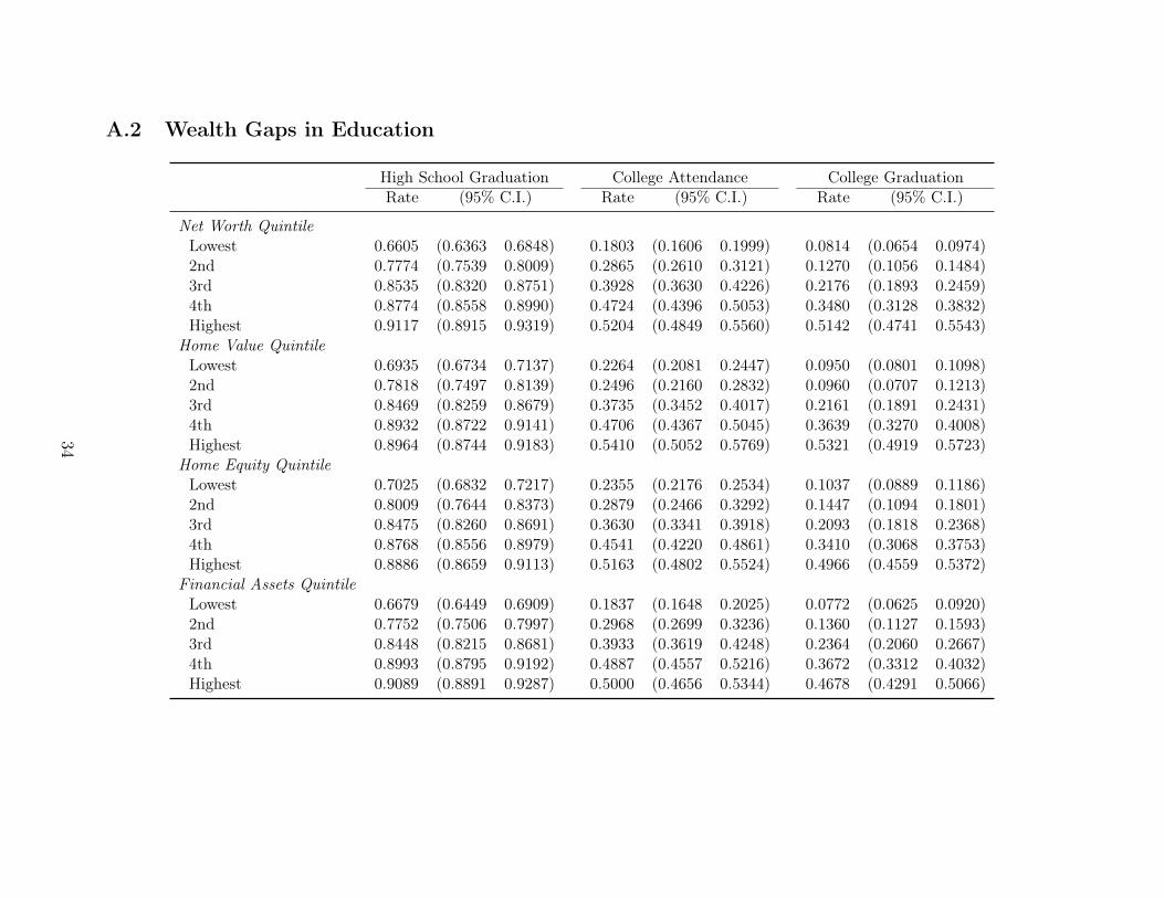
and reported in Appendix A.2.

The PSID wealth measures have been shown to have high validity though they do not

capture the very top (2-3 percent) of the wealth distribution well (Juster et al. 1999; Pf-

effer et al. 2016). Since this study focuses on population associations between wealth and

education rather than the educational pathways of children of a small wealth elite (for the

latter see, e.g., Khan 2012), this shortcoming is less problematic and likely results in a con-

servative estimate of the educational advantages among the top wealth group assessed here.

In fact, the main specification of wealth gaps reported here draws on wealth quintiles to

capture non-linearities in intergenerational associations throughout the distribution but not

8

necessarily the very top.6 Quintiles are drawn within each cohort and based on the weighted

analytic sample; unweighted quintiles yield similar results.

This study also uses a comprehensive set of indicators of the socio-economic position of

families besides family wealth. As a measure of permanent income, I use total household

income averaged across five income years (in quintiles; alternative specifications again include

log-transformed versions). The indicator of educational backgrounds are measured as the

highest degree attained by either the household head or partner. Occupational background is

measured as the highest socio-economic index score (SEI) of either head’s or partner’s main

occupation. Further controls for demographic characteristics include the household size,

the number of children in the household, whether the household head is married, mother’s

age, individuals’ sex, and the source of information for their educational outcomes (self-

reported or not). Each of these yearly measures is drawn from the same survey wave as

the wealth measure (1984, 1989, 1994, 1999). The main predictor of college attainment

studied here, family wealth (as well as family income), is provided in imputed form by the

PSID; few missing values on all remaining predictors are multiply imputed using Stata’s mi

procedures. A small share of cases (less than 1 percent) with imputed dependent variables are

dropped (von Hippel 2007). Descriptive statistics for all variables included in this analysis

are reported in Appendix A.1. All dollar values are inflation adjusted to 2013.

Wealth gaps in high school attainment, college access, and bachelor’s degree attainment

are estimated via logistic regressions. I begin by describing observed rates of educational

attainment by family wealth quintile. Next, I estimate adjusted rates based on models

including the control variables mentioned above. I report predictive margins and, for the

cohort comparison, discrete changes based on average marginal effects (see Hanmer and

Ozan Kalkan 2013) using Stata’s margin commands. The approach to estimate to which

extent changes in the wealth distribution account for trends in wealth gaps in education is6Other specifications tested (available upon request) include the inverse hyperbolic sine transformation

(see Burbidge et al. 1988), which – like the quintiles specification reported here – retains non-positive networth values, and log-transformed specifications with and without a floor value for cases of zero or net debtand with top-coding to reduce the undue influence of outliers.

9

targeted to explain a specific trend revealed in the preceding analyses and therefore described

later. The regression results reported here are unweighted but results are very stable to the

use of individual and family weights provided by the PSID.

Findings

Wealth gaps in educational attainment

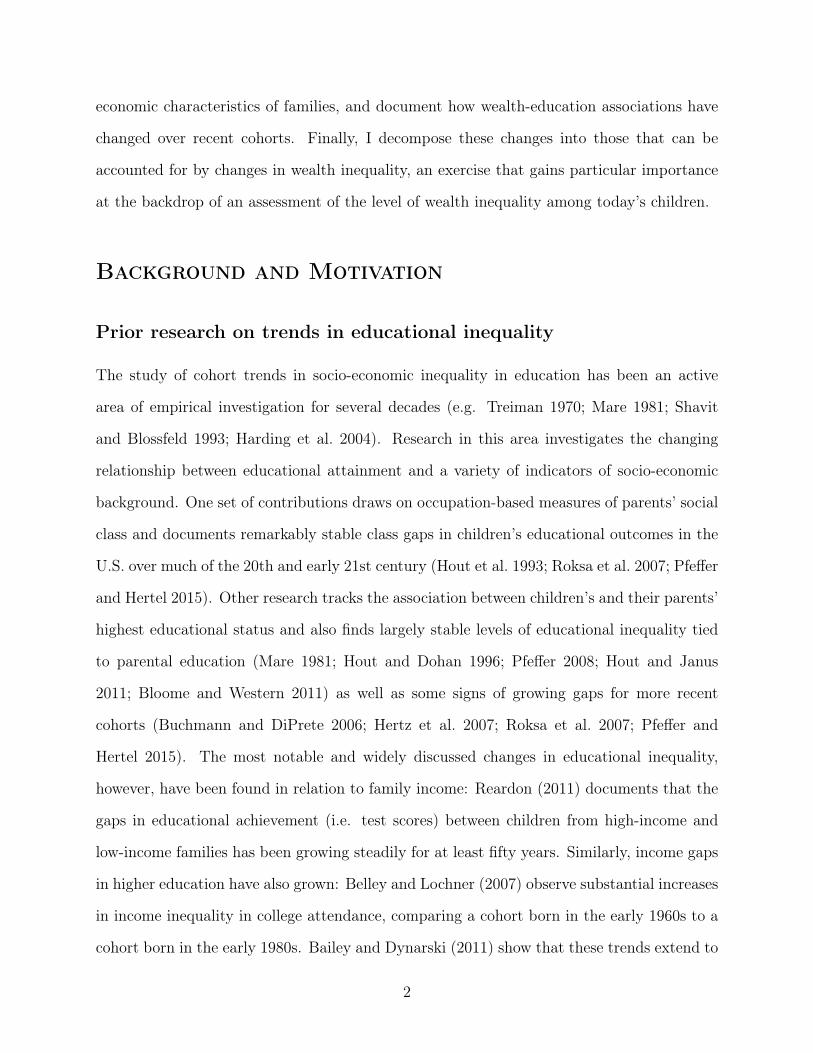
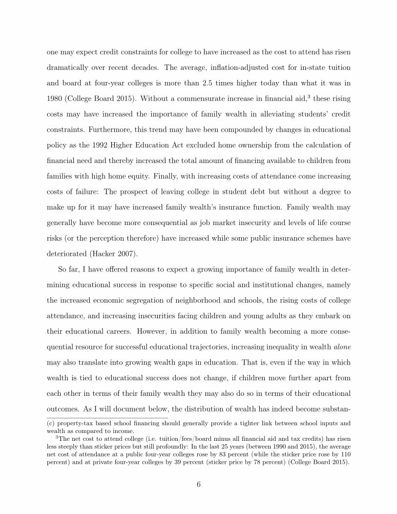
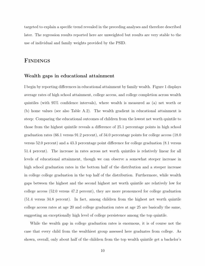
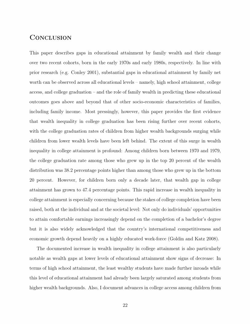
I begin by reporting differences in educational attainment by family wealth. Figure 1 displays

average rates of high school attainment, college access, and college completion across wealth

quintiles (with 95% confidence intervals), where wealth is measured as (a) net worth or

(b) home values (see also Table A.2). The wealth gradient in educational attainment is

steep: Comparing the educational outcomes of children from the lowest net worth quintile to

those from the highest quintile reveals a difference of 25.1 percentage points in high school

graduation rates (66.1 versus 91.2 percent), of 34.0 percentage points for college access (18.0

versus 52.0 percent) and a 43.3 percentage point difference for college graduation (8.1 versus

51.4 percent). The increase in rates across net worth quintiles is relatively linear for all

levels of educational attainment, though we can observe a somewhat steeper increase in

high school graduation rates in the bottom half of the distribution and a steeper increase

in college college graduation in the top half of the distribution. Furthermore, while wealth

gaps between the highest and the second highest net worth quintile are relatively low for

college access (52.0 versus 47.2 percent), they are more pronounced for college graduation

(51.4 versus 34.8 percent). In fact, among children from the highest net worth quintile

college access rates at age 20 and college graduation rates at age 25 are basically the same,

suggesting an exceptionally high level of college persistence among the top quintile.

While the wealth gap in college graduation rates is enormous, it is of course not the

case that every child from the wealthiest group assessed here graduates from college. As

shown, overall, only about half of the children from the top wealth quintile get a bachelor’s

10

Figure 1: Educational Rates by Wealth Background

(a) (b)0

.1.2

.3.4

.5.6

.7.8

.91

Rate

s

Lowest 2nd 3rd 4th HighestNet Worth Quintiles

0.1

.2.3

.4.5

.6.7

.8.9

1R

ate

s

Lowest 2nd 3rd 4th HighestHome Value Quintiles

High School College Attendance BA

degree. That should not comes as a surprise to those familiar with estimates of college

graduation rate among recent U.S. cohorts, which closely resemble those estimated here.7

With overall graduation rates at age 25 below 30 percent, even if no child from the bottom

half of the wealth distribution were to graduate from college, one would still expect college

graduation rates of less than 60 percent in the top half of the distribution. While it is thus a

misperception that a great majority of children from wealthy households graduate college, it

is certainly the case that the modal college graduate comes from a household with significant

net worth. In this analytic sample, half of all college graduates come from a household with7Based on the Current Population Survey March Supplement, I estimate a college graduation rate for

comparable individuals – specifically, individuals who are heads of households and age 25 in survey years1995 through 2009 – of 28 percent compared to 26 percent based on the analytic sample used here.

11

more than $180,000 in net worth and a full fifth of them come from a household with at

least half a million dollar net worth.

In addition to the assessment of gaps by families’ net worth, Figure 1b also displays edu-

cational rates by home value quintiles.8 The degree and pattern of inequality in educational

attainment by families’ home values closely approximates those by families’ net worth (Fig-

ure 1a). Though other wealth components, such as financial assets or home equity (home

values minus mortgages), fare similarly well in approximating the reported net worth gaps

(see Table A.2), home values provide in many ways the most attractive proxy measure. Sub-

stantively, home ownership constitutes the main asset component in most families’ wealth

portfolio. From a measurement perspective, home values are the easiest to collect among

all asset components and, as such, appear to be a promising candidate to help remedy the

data shortage that so far has hampered work on the relationship between family wealth and

educational outcomes.

Wealth as an independent source of educational advantage

The large wealth gaps in educational outcomes described above can, of course, also arise

from other correlated characteristics, not the least other socio-economic factors. Accord-

ingly, the observed wealth gaps in education discussed above – and again displayed in Table

1, column “Unconditional” – are lower once controls for observable characteristics of parents

and children are added (see list of controls discussed above). Still, wealth gaps in education

adjusted for these controls (Table 1, column “Conditional”) remain statistically and substan-

tively significant: All else equal, the gap in educational attainment between children from

the bottom quintile and children from the top quintile of the net worth distribution still

(statistically significantly) differs by 10.5 percentage points for high school graduation, 8.2

percentage points for college access, and 8.0 percentage points for college graduation.8Here, the lowest group contains those whose parents do not own a home (home value of zero), about 30

percent of the sample, while the second lowest group (about 10 percent of the sample) consists of childrenfrom owned homes valued at most about $62,900 (see Table A.1). The remaining groups are standard

12

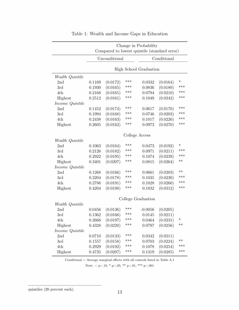
Table 1: Wealth and Income Gaps in Education

Change in ProbabilityCompared to lowest quintile (standard error)

Unconditional Conditional

High School Graduation

Wealth Quintile2nd 0.1169 (0.0172) *** 0.0332 (0.0164) *3rd 0.1930 (0.0165) *** 0.0836 (0.0180) ***4th 0.2168 (0.0165) *** 0.0794 (0.0210) ***Highest 0.2512 (0.0161) *** 0.1049 (0.0242) ***

Income Quintile2nd 0.1452 (0.0174) *** 0.0617 (0.0170) ***3rd 0.1994 (0.0168) *** 0.0746 (0.0203) ***4th 0.2438 (0.0163) *** 0.1017 (0.0226) ***Highest 0.2605 (0.0162) *** 0.0973 (0.0270) ***

College AccessWealth Quintile2nd 0.1063 (0.0164) *** 0.0473 (0.0192) *3rd 0.2126 (0.0182) *** 0.0971 (0.0211) ***4th 0.2922 (0.0195) *** 0.1074 (0.0239) ***Highest 0.3401 (0.0207) *** 0.0815 (0.0264) **

Income Quintile2nd 0.1268 (0.0166) *** 0.0661 (0.0203) **3rd 0.2204 (0.0178) *** 0.1035 (0.0230) ***4th 0.2786 (0.0191) *** 0.1028 (0.0260) ***Highest 0.4204 (0.0198) *** 0.1832 (0.0312) ***

College GraduationWealth Quintile2nd 0.0456 (0.0136) *** -0.0056 (0.0205)3rd 0.1362 (0.0166) *** 0.0145 (0.0211)4th 0.2666 (0.0197) *** 0.0464 (0.0231) *Highest 0.4328 (0.0220) *** 0.0797 (0.0256) **

Income Quintile2nd 0.0710 (0.0133) *** 0.0342 (0.0211)3rd 0.1557 (0.0158) *** 0.0703 (0.0224) **4th 0.2929 (0.0192) *** 0.1078 (0.0254) ***Highest 0.4735 (0.0207) *** 0.1319 (0.0285) ***

Conditional = Average marginal effects with all controls listed in Table A.1

Note: + p<.10, * p<.05, ** p<.01, *** p<.001

quintiles (20 percent each).13

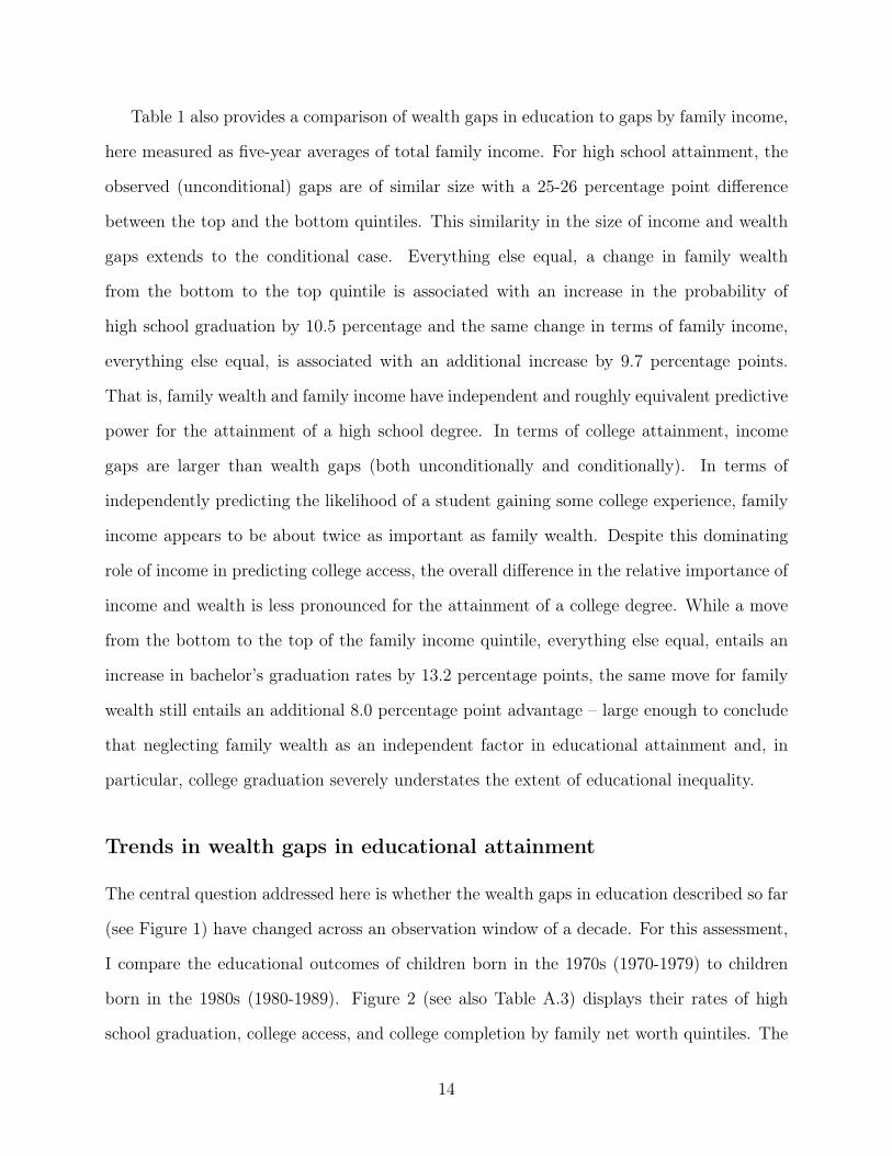
Table 1 also provides a comparison of wealth gaps in education to gaps by family income,

here measured as five-year averages of total family income. For high school attainment, the

observed (unconditional) gaps are of similar size with a 25-26 percentage point difference

between the top and the bottom quintiles. This similarity in the size of income and wealth

gaps extends to the conditional case. Everything else equal, a change in family wealth

from the bottom to the top quintile is associated with an increase in the probability of

high school graduation by 10.5 percentage and the same change in terms of family income,

everything else equal, is associated with an additional increase by 9.7 percentage points.

That is, family wealth and family income have independent and roughly equivalent predictive

power for the attainment of a high school degree. In terms of college attainment, income

gaps are larger than wealth gaps (both unconditionally and conditionally). In terms of

independently predicting the likelihood of a student gaining some college experience, family

income appears to be about twice as important as family wealth. Despite this dominating

role of income in predicting college access, the overall difference in the relative importance of

income and wealth is less pronounced for the attainment of a college degree. While a move

from the bottom to the top of the family income quintile, everything else equal, entails an

increase in bachelor’s graduation rates by 13.2 percentage points, the same move for family

wealth still entails an additional 8.0 percentage point advantage – large enough to conclude

that neglecting family wealth as an independent factor in educational attainment and, in

particular, college graduation severely understates the extent of educational inequality.

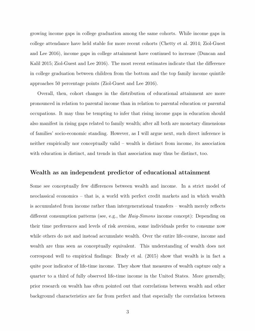
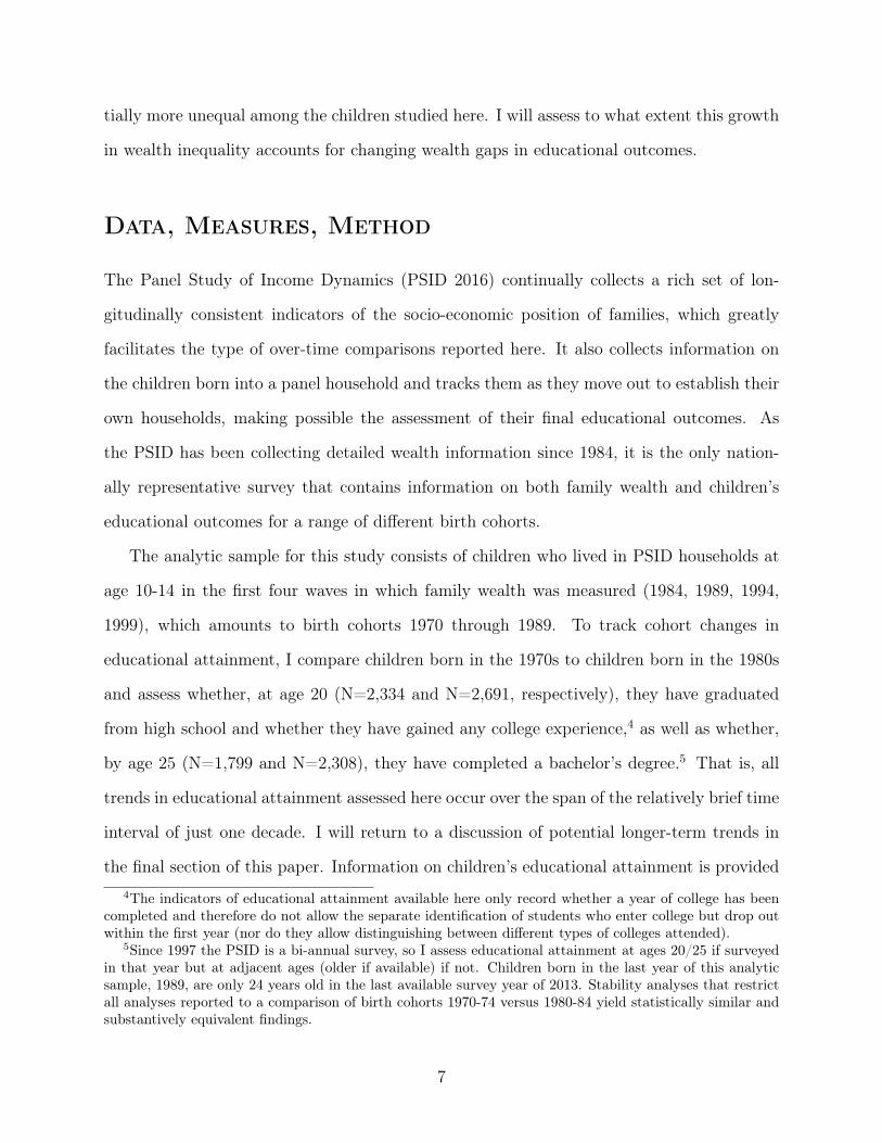
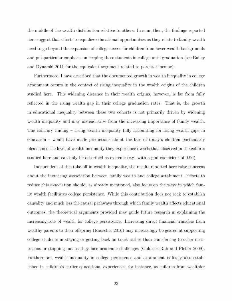
Trends in wealth gaps in educational attainment

The central question addressed here is whether the wealth gaps in education described so far

(see Figure 1) have changed across an observation window of a decade. For this assessment,

I compare the educational outcomes of children born in the 1970s (1970-1979) to children

born in the 1980s (1980-1989). Figure 2 (see also Table A.3) displays their rates of high

school graduation, college access, and college completion by family net worth quintiles. The

14

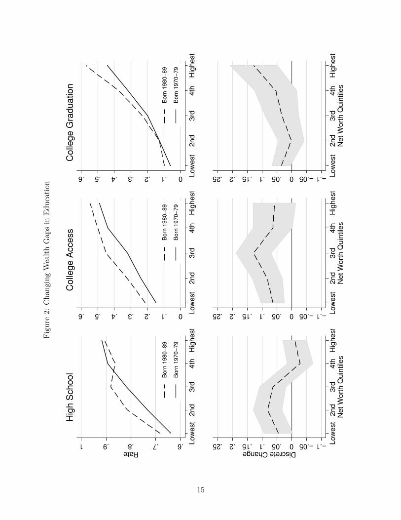
Figure2:

Cha

ngingWealthGap

sin

Edu

cation

.6.7.8.91Rate

Lo

we

st

2n

d3

rd4

thH

igh

est

Bo

rn 1

98

0−

89

Bo

rn 1

97

0−

79

Hig

h S

chool

0.1.2.3.4.5.6 Lo

we

st

2n

d3

rd4

thH

igh

est

Bo

rn 1

98

0−

89

Bo

rn 1

97

0−

79

Colle

ge A

ccess

0.1.2.3.4.5.6 Lo

we

st

2n

d3

rd4

thH

igh

est

Bo

rn 1

98

0−

89

Bo

rn 1

97

0−

79

Colle

ge G

raduation

−.1−.050.05.1.15.2.25Discrete Change

Lo

we

st

2n

d3

rd4

thH

igh

est

Ne

t W

ort

h Q

uin

tile

s

−.1−.050.05.1.15.2.25 Lo

we

st

2n

d3

rd4

thH

igh

est

Ne

t W

ort

h Q

uin

tile

s−.1−.050.05.1.15.2.25 L

ow

est

2n

d3

rd4

thH

igh

est

Ne

t W

ort

h Q

uin

tile

s

15

upper panel reports the graduation rates separately for these two cohorts while the lower

panel displays the difference in graduation rates with the earlier born cohort as the reference

and 95% confidence intervals to allow the assessment of statistical significance of cohort

differences (see Long and Freese 2014: p. 297ff on why statistical significance tests should

be based on estimates of discrete change).

Starting with high school attainment, we observe that average graduation rates have in-

creased between these two cohorts for students from the bottom three wealth quintiles. For

instance, children in the more recent cohort who grew up in the middle fifth of the wealth

distribution have a graduation rate of 88.2 percent, which is 6.3 percentage points above that

of students from the middle fifth of the wealth distribution born a decade earlier. The high

school attainment of students from the top two wealth quintiles, in contrast, has not changed

in this time frame, a potential sign of saturation of this educational level among wealthier

households. Overall, then, with the bottom 60 percent increasing their high school gradua-

tion rate and the top 40 percent largely stable, wealth inequality in high school attainment

has decreased.

We also observe some signs of equalization in terms of college access: College access rates

have improved between these two cohorts for children from the bottom three quintiles – and

most notably, with an increase of 12.9 percentage points (from 32.2 to 45.1 percent), for

children from the middle quintile – while college access rates expanded at a less rapid rate

– with a statistically insignificant increase of about 6 percentage points – for the top two

quintiles.

Trends in college attainment are very different and stark. Children from the bottom

60 percent of the wealth distribution were not able to make much progress over the decade

studied here (0 to 3.5 percentage point increase) and children from the next 20 percent of the

wealth distribution increased their college completion rates by 5.3 percentage points. The

most marked increase, however, was experienced by children from the top 20 percent of the

distribution. With an increase in the college graduation rate of 12.7 percentage points in the

16

span of just a decade, the wealthiest children have pulled away from others in terms of college

attainment. That is, despite some decreases in wealth gaps in high school attainment and

college access, the clearest and largest change in the distribution of educational opportunity

lies in the rising gap between those from the top 20 percent of the wealth distribution and

everyone else. As a result, while college graduation rates between those from the top and the

bottom quintile of the wealth distribution differed by 38.2 percentage points among children

who born in the 1970s, it differed by a full 47.4 percentage points for children born a decade

later; a growth of the wealth gap in college attainment by 9.2 percentage points in just a

decade.

Growing wealth gaps in college graduation in the context of rising

wealth inequality

In the remainder, I will focus on the growing wealth gap in college completion – as the most

concerning finding yielded by the analyses provided above – and assess to what degree it is

related to the growth in wealth inequality. As argued above, while wealth may have become

a more influential factor in determining college success, the fact alone that those at the top

of the distribution have increasingly more wealth at their disposal than everyone else may

also account for some of the growth in wealth inequality in education. I begin by describing

the growth of wealth inequality among the children of the two cohorts studied here and also

report on levels of wealth inequality among today’s children (aged 10-14 in the the latest

available survey wave of 2013). I then describe the decomposition approach used to estimate

the degree to which the observed rise in wealth inequality contributes to the documented

increase in the wealth gap in college attainment.

Table 2 reports the median wealth among three groups of children: Those growing up in

the bottom 80 percent of the family wealth distribution, the next ten percent, and the top

ten percent. The differences in family wealth between these three groups are already high

for the first cohort studied here: The typical family net worth of children in the bottom four

17

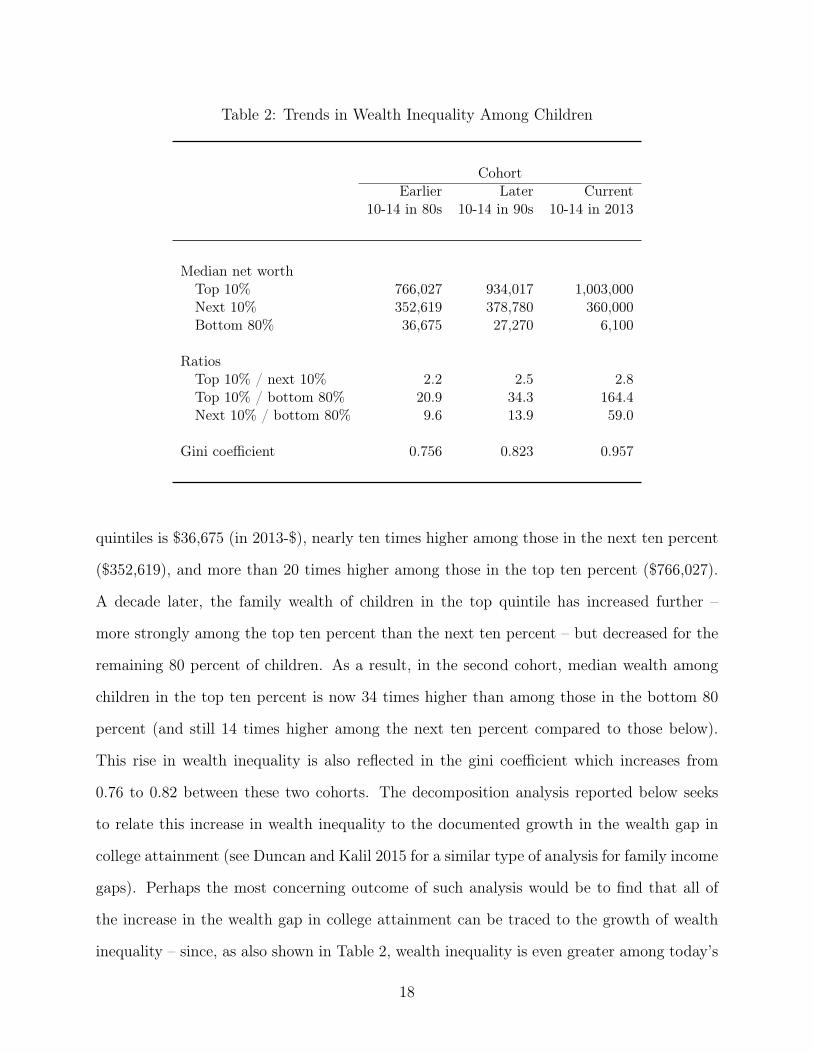
Table 2: Trends in Wealth Inequality Among Children

CohortEarlier Later Current

10-14 in 80s 10-14 in 90s 10-14 in 2013

Median net worthTop 10% 766,027 934,017 1,003,000Next 10% 352,619 378,780 360,000Bottom 80% 36,675 27,270 6,100

RatiosTop 10% / next 10% 2.2 2.5 2.8Top 10% / bottom 80% 20.9 34.3 164.4Next 10% / bottom 80% 9.6 13.9 59.0

Gini coefficient 0.756 0.823 0.957

quintiles is $36,675 (in 2013-$), nearly ten times higher among those in the next ten percent

($352,619), and more than 20 times higher among those in the top ten percent ($766,027).

A decade later, the family wealth of children in the top quintile has increased further –

more strongly among the top ten percent than the next ten percent – but decreased for the

remaining 80 percent of children. As a result, in the second cohort, median wealth among

children in the top ten percent is now 34 times higher than among those in the bottom 80

percent (and still 14 times higher among the next ten percent compared to those below).

This rise in wealth inequality is also reflected in the gini coefficient which increases from

0.76 to 0.82 between these two cohorts. The decomposition analysis reported below seeks

to relate this increase in wealth inequality to the documented growth in the wealth gap in

college attainment (see Duncan and Kalil 2015 for a similar type of analysis for family income

gaps). Perhaps the most concerning outcome of such analysis would be to find that all of

the increase in the wealth gap in college attainment can be traced to the growth of wealth

inequality – since, as also shown in Table 2, wealth inequality is even greater among today’s

18

children. Among children observed in the latest available PSID wave of 2013, wealth is even

more heavily concentrated at the top: Children in the top ten percent of the distribution

now typically grow up with about $1 million in net worth, about 164 times the wealth of

the remaining 80 percent of children whose typical family wealth is a meager $6,100. The

gini coefficient has risen to 0.96, remarkably close to the scenario of complete inequality

henceforth reserved to didactic examples of how to interpret a gini coefficient of one. At the

backdrop of such extreme level of wealth inequality among today’s children, the growth in

wealth inequality among earlier cohorts appears relatively low. Still, knowing whether this

growth can be traced to the college outcomes of these children may inform our expectations

about the fate of today’s children.

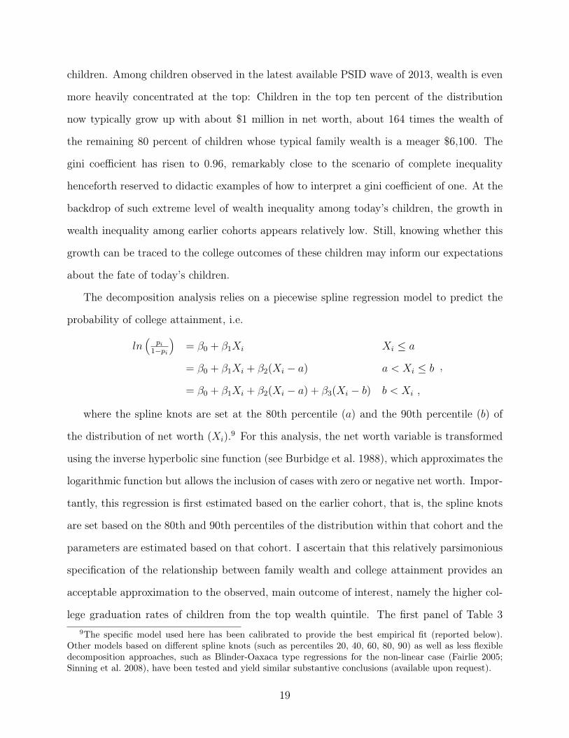
The decomposition analysis relies on a piecewise spline regression model to predict the

probability of college attainment, i.e.

ln(

pi1−pi

)= β0 + β1Xi Xi ≤ a

= β0 + β1Xi + β2(Xi − a) a < Xi ≤ b

= β0 + β1Xi + β2(Xi − a) + β3(Xi − b) b < Xi ,

,

where the spline knots are set at the 80th percentile (a) and the 90th percentile (b) of

the distribution of net worth (Xi).9 For this analysis, the net worth variable is transformed

using the inverse hyperbolic sine function (see Burbidge et al. 1988), which approximates the

logarithmic function but allows the inclusion of cases with zero or negative net worth. Impor-

tantly, this regression is first estimated based on the earlier cohort, that is, the spline knots

are set based on the 80th and 90th percentiles of the distribution within that cohort and the

parameters are estimated based on that cohort. I ascertain that this relatively parsimonious

specification of the relationship between family wealth and college attainment provides an

acceptable approximation to the observed, main outcome of interest, namely the higher col-

lege graduation rates of children from the top wealth quintile. The first panel of Table 39The specific model used here has been calibrated to provide the best empirical fit (reported below).

Other models based on different spline knots (such as percentiles 20, 40, 60, 80, 90) as well as less flexibledecomposition approaches, such as Blinder-Oaxaca type regressions for the non-linear case (Fairlie 2005;Sinning et al. 2008), have been tested and yield similar substantive conclusions (available upon request).

19

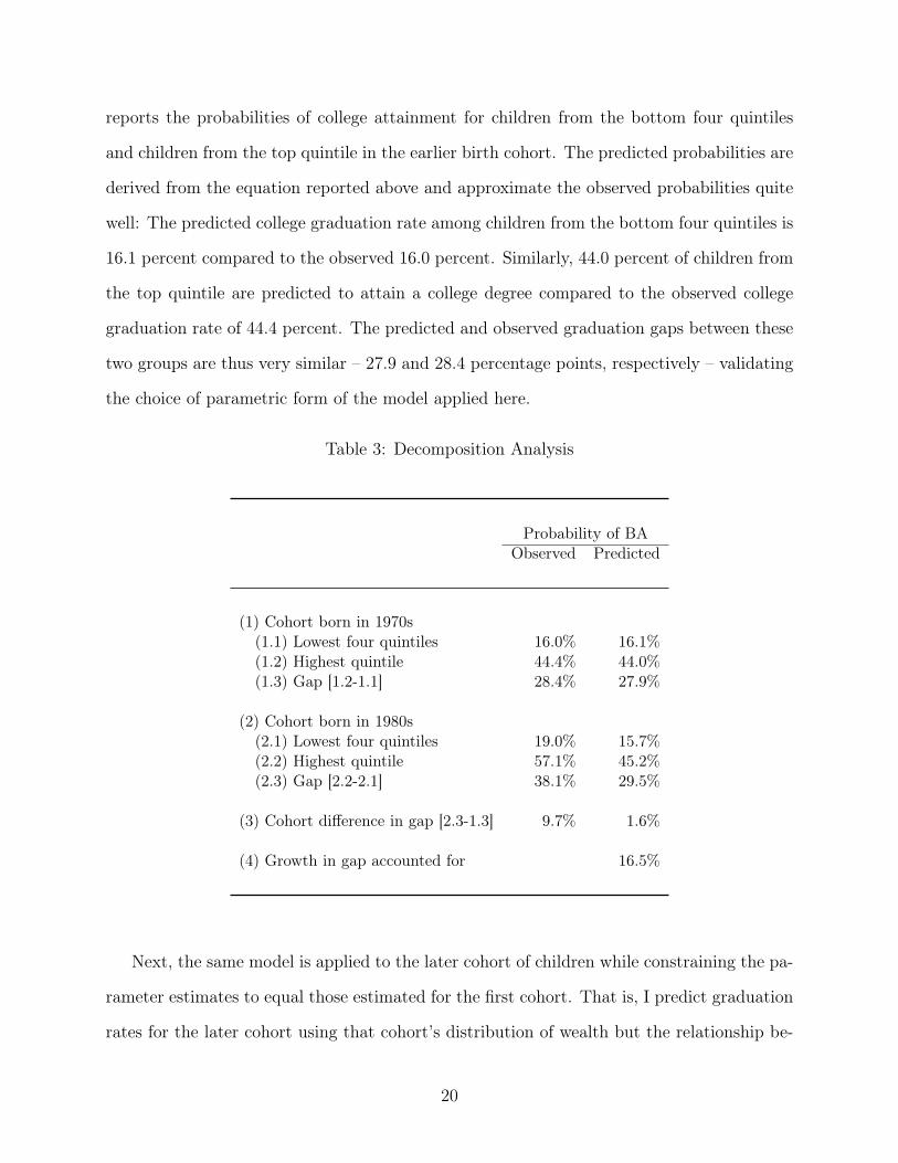
reports the probabilities of college attainment for children from the bottom four quintiles

and children from the top quintile in the earlier birth cohort. The predicted probabilities are

derived from the equation reported above and approximate the observed probabilities quite

well: The predicted college graduation rate among children from the bottom four quintiles is

16.1 percent compared to the observed 16.0 percent. Similarly, 44.0 percent of children from

the top quintile are predicted to attain a college degree compared to the observed college

graduation rate of 44.4 percent. The predicted and observed graduation gaps between these

two groups are thus very similar – 27.9 and 28.4 percentage points, respectively – validating

the choice of parametric form of the model applied here.

Table 3: Decomposition Analysis

Probability of BAObserved Predicted

(1) Cohort born in 1970s(1.1) Lowest four quintiles 16.0% 16.1%(1.2) Highest quintile 44.4% 44.0%(1.3) Gap [1.2-1.1] 28.4% 27.9%

(2) Cohort born in 1980s(2.1) Lowest four quintiles 19.0% 15.7%(2.2) Highest quintile 57.1% 45.2%(2.3) Gap [2.2-2.1] 38.1% 29.5%

(3) Cohort difference in gap [2.3-1.3] 9.7% 1.6%

(4) Growth in gap accounted for 16.5%

Next, the same model is applied to the later cohort of children while constraining the pa-

rameter estimates to equal those estimated for the first cohort. That is, I predict graduation

rates for the later cohort using that cohort’s distribution of wealth but the relationship be-

20

tween wealth and college outcomes as observed in the earlier cohort. If the changing wealth

gap in college attainment was entirely driven by the change in wealth inequality between

these two cohorts, this prediction should come close to the wealth gap in college observed

for the second cohort. However, as shown in the second panel of Table 3, the predicted and

observed wealth gaps in college graduation diverge from each other, mostly because apply-

ing the wealth effects estimated in the earlier cohort to the wealth distribution of the later

cohort underestimates the college attainment of the top quintile (45.2 percent versus 57.1

percent), that is, it misses most of the surge in college attainment at the top established

in the prior section. As a result, the predicted wealth gap in college attainment is much

smaller than observed (29.5 vs. 38.1 percentage points). While the wealth gap in college

attainment between the top quintile and everyone else rose by 9.7 percentage points between

these two cohorts, the rise predicted by assuming a stable association between wealth and

college attainment is only 1.6 percentage points.

Overall, then, the conclusion is that the rise in wealth inequality alone explains only a

small share – about one sixth (16.5 percent) – of the growth in the gap in college attainment

between the wealthiest 20 percent of students and the rest. Put differently, the increase in

wealth gaps between these two cohorts is not fully reflected in the increase in wealth gaps

in their later college attainment, which may qualify as good news at the backdrop of the

extreme level of wealth inequality among today’s children. Given this result, it does not

seem reasonable to interpolate from the gaps in college attainment observed here to gaps in

the future college attainment of today’s children based on the level of wealth inequality they

experience. Still, the possibility that the growing inequality in college attainment stems

primarily from changes in the importance of wealth for college success (rather than from

changes in the distribution of wealth), should encourage policy efforts geared at reducing

the inequitable effects of wealth on educational attainment. Short of such changes, today’s

children can be expected to suffer at least as much inequality in their college opportunities

as the children studied here.

21

Conclusion

This paper describes gaps in educational attainment by family wealth and their change

over two recent cohorts, born in the early 1970s and early 1980s, respectively. In line with

prior research (e.g. Conley 2001), substantial gaps in educational attainment by family net

worth can be observed across all educational levels – namely, high school attainment, college

access, and college graduation – and the role of family wealth in predicting these educational

outcomes goes above and beyond that of other socio-economic characteristics of families,

including family income. Most pressingly, however, this paper provides the first evidence

that wealth inequality in college graduation has been rising further over recent cohorts,

with the college graduation rates of children from higher wealth backgrounds surging while

children from lower wealth levels have been left behind. The extent of this surge in wealth

inequality in college attainment is profound: Among children born between 1970 and 1979,

the college graduation rate among those who grew up in the top 20 percent of the wealth

distribution was 38.2 percentage points higher than among those who grew up in the bottom

20 percent. However, for children born only a decade later, that wealth gap in college

attainment has grown to 47.4 percentage points. This rapid increase in wealth inequality in

college attainment is especially concerning because the stakes of college completion have been

raised, both at the individual and at the societal level: Not only do individuals’ opportunities

to attain comfortable earnings increasingly depend on the completion of a bachelor’s degree

but it is also widely acknowledged that the country’s international competitiveness and

economic growth depend heavily on a highly educated work-force (Goldin and Katz 2008).

The documented increase in wealth inequality in college attainment is also particularly

notable as wealth gaps at lower levels of educational attainment show signs of decrease: In

terms of high school attainment, the least wealthy students have made further inroads while

this level of educational attainment had already been largely saturated among students from

higher wealth backgrounds. Also, I document advances in college access among children from

22

the middle of the wealth distribution relative to others. In sum, then, the findings reported

here suggest that efforts to equalize educational opportunities as they relate to family wealth

need to go beyond the expansion of college access for children from lower wealth backgrounds

and put particular emphasis on keeping these students in college until graduation (see Bailey

and Dynarski 2011 for the equivalent argument related to parental income).

Furthermore, I have described that the documented growth in wealth inequality in college

attainment occurs in the context of rising inequality in the wealth origins of the children

studied here. This widening distance in their wealth origins, however, is far from fully

reflected in the rising wealth gap in their college graduation rates. That is, the growth

in educational inequality between these two cohorts is not primarily driven by widening

wealth inequality and may instead arise from the increasing importance of family wealth.

The contrary finding – rising wealth inequality fully accounting for rising wealth gaps in

education – would have made predictions about the fate of today’s children particularly

bleak since the level of wealth inequality they experience dwarfs that observed in the cohorts

studied here and can only be described as extreme (e.g. with a gini coefficient of 0.96).

Independent of this take-off in wealth inequality, the results reported here raise concerns

about the increasing association between family wealth and college attainment. Efforts to

reduce this association should, as already mentioned, also focus on the ways in which fam-

ily wealth facilitates college persistence. While this contribution does not seek to establish

causality and much less the causal pathways through which family wealth affects educational

outcomes, the theoretical arguments provided may guide future research in explaining the

increasing role of wealth for college persistence: Increasing direct financial transfers from

wealthy parents to their offspring (Rauscher 2016) may increasingly be geared at supporting

college students in staying or getting back on track rather than transferring to other insti-

tutions or stopping out as they face academic challenges (Goldrick-Rab and Pfeffer 2009).

Furthermore, wealth inequality in college persistence and attainment is likely also estab-

lished in children’s earlier educational experiences, for instance, as children from wealthier

23

households attend high schools that leave them academically better prepared for college and

thereby also facilitate access to colleges with higher retention rates, such as highly competi-

tive and prestigious four-year schools (Bastedo and Jaquette 2011).

This last observation also points to one of the limitations of this contribution and op-

portunities for future research: This study does not investigate “horizontal” differences in

education, for instance, wealth gaps by institution type and selectivity (but see Jez 2014).

Yet, as children from the wealthiest families have reached saturation of educational partici-

pation at the secondary level and more children from wealth backgrounds below the top are

accessing higher education (as documented here), the wealthiest households may increasingly

exploit these types of horizontal differences in the educational system to effectively maintain

inequality (Lucas 2001; Gerber and Cheung 2008). In this sense, the growth of wealth in-

equality in college outcomes shown here may still provide a conservative estimate. Another

way in which this analysis may underestimate the degree of wealth inequality in education is

through its exclusive focus on the immediate family: Advantages arising from family wealth

may extend beyond the parent-child dyad as the wealth of grandparents or even wealth in

extended family networks may additionally facilitate educational success (Roksa and Potter

2011; Prix and Pfeffer 2017). Revealingly, many college campuses around the country have

begun to complement their family visit day with a portion dedicated to grandparents (e.g.

Feiler 2014).

Finally, the finding that home values serve as a powerful proxy measure of wealth gaps in

education may be particularly important to help expand the research base and facilitate fu-

ture research. Home value indicators are more easily collected than full-fledged asset survey

modules to measure total family net worth and often readily accessible through administra-

tive or linked external data. For instance, drawing on home values to approximate wealth

gaps in education may allow historical assessments of wealth inequality in education (e.g.

based on the housing values reported on the publicly available 1940 Census), longer-term

assessments of additional cohorts (e.g. based on the housing information consistently ob-

24

served in the PSID since 1968), or detailed analysis of wealth gaps in college pathways based

on administrative data held by colleges and states that also include the addresses of stu-

dents’ pre-college residence (for which external real estate data yield home value estimates).

Of course, the documented role of home values in approximating wealth gaps in education

goes beyond a measurement issue. It poses the question to what extent wealth effects on

education are in fact asset effects, effects of housing quality (e.g., Lopoo and London 2016),

and effects of the neighborhoods in which highly-valued houses are located (Sampson et al.

2002; Durlauf 2004). The broad but largely separate literatures that exist on each of these

potential channels that link housing wealth to educational success urgently await integration.

25

References

Axinn, William, Greg J. Duncan, and Arland Thornton. 1997. “The Effects of Parents’Income, Wealth and Attitudes on Children’s Completed Schooling and Self-Esteem.” InConsequences of Growing Up Poor , edited by Greg J. Duncan and Jeanne Brooks-Gunn,pp. 518–540. New York: Russell Sage Foundation.

Bailey, Martha J. and Susan M. Dynarski. 2011. “Inequality in Postsecondary Education.”In Whither Opportunity? Rising Inequality, Schools, and Children’s Life Chances , editedby Greg J. Duncan and Richard J. Murnane, pp. 117–131. New York: Russell Sage Foun-dation.

Bastedo, M. N. and O. Jaquette. 2011. “Running in Place: Low-Income Students and theDynamics of Higher Education Stratification.” Educational Evaluation and Policy Analysis33:318–339.

Belley, Philippe and Lance Lochner. 2007. “The Changing Role of Family Income and Abilityin Determining Educational Achievement.” Journal of Human Capital 1:37–89.

Bloome, D. and B. Western. 2011. “Cohort Change and Racial Differences in Educationaland Income Mobility.” Social Forces 90:375–395.

Brady, David, Anke Radenacker, Marco Giesselmann, and Ulrich Kohler. 2015. “ProxyingPermanent Income in Germany and U.S.” Unpublished Manuscript .

Buchmann, Claudia, Dennis Condron, and Vincent Roscigno. 2010. “Shadow Education,American Style. Test Preparation, the SAT and College Enrollment.” Social Forces 89:435–462.

Buchmann, Claudia and Thomas A DiPrete. 2006. “The Growing Female Advantage in Col-lege Completion. The Role of Family Background and Academic Achievement.” AmericanSociological Review 71:515–541.

Burbidge, John B., Lonnie Magee, and A. Leslie Robb. 1988. “Alternative Transformationsto Handle Extreme Values of the Dependent Variable.” Journal of the American StatisticalAssociation 83:123–127.

Cameron, Stephen V and Christopher Taber. 2004. “Estimation of Educational BorrowingConstraints Using Returns to Schooling.” Journal of Political Economy 112:132–182.

Chetty, Raj, Nathaniel Hendren, Patrick Kline, Emmanuel Saez, and Nicholas Turner. 2014.“Is the United States still a land of opportunity? Recent trends in intergenerational mo-bility.” NBER Working Paper Series 19844.

\{College Board\}. 2015. Trends in College Pricing . New York: The College Board.

Conley, Dalton. 1999. Being Black, Living in the Red. Race, Wealth, and Social Policy inAmerica. Berkeley: University of California Press.

26

Conley, Dalton. 2001. “Capital for College. Parental Assets and Postsecondary Schooling.”Sociology of Education 74:59–72.

Duncan, Greg J and Ariel Kalil. 2015. “Increasing Inequality in Parent Incomes and Chil-dren’s Completed Schooling: Correlation or Causation?” Unpublished Manuscript .

Durlauf, Steven N. 2004. “Neighborhood Effects.” In Handbook of Regional and UrbanEconomics , edited by J. Vernon Henderson and Jacques-Francois Thisse, volume 4, pp.2173–2242. Elsevier.

Fairlie, Robert W. 2005. “An extension of the Blinder-Oaxaca decomposition technique tologit and probit models.” Journal of Economic and Social Measurement 30:305–316.

Feiler, Bruce. 2014. “College Family Weekend Isn’t Just for Parents Anymore.” The NewYork Times .

Gerber, Theodore P. and Sin Yi Cheung. 2008. “Horizontal Stratification in PostsecondaryEducation. Forms, Explanations, and Implications.” Annual Review of Sociology 34:299–318.

Goldin, Claudia and Lawrence F. Katz. 2008. The Race between Education and Technology .Cambridge: Harvard University Press.

Goldrick-Rab, Sara and Fabian T. Pfeffer. 2009. “Beyond Access. Explaining SocioeconomicDifferences in College Transfer.” Sociology of Education 82:101–125.

Hacker, Jacob S. 2007. The Great Risk Shift. The New Economic Insecurity and the Declineof the American Dream. Oxford: Oxford University Press.

Hanmer, Michael J. and Kerem Ozan Kalkan. 2013. “Behind the Curve. Clarifying theBest Approach to Calculating Predicted Probabilities and Marginal Effects from LimitedDependent Variable Models.” American Journal of Political Science 57:263–277.

Harding, David J., Christopher Jencks, Leonard M. Lopoo, and Susan E. Mayer. 2004. “TheChanging Effect of Family Background on the Incomes of American Adults.” In UnequalChances: Family Background and Economic Success , edited by Samuel Bowles, HerbertGintis, and Anastasiya M. Osborne. Princeton: Princeton University Press.

Haurin, Donald R, Toby L Parcel, and R Jean Haurin. 2002. “Does Homeownership AffectChild Outcomes?” Real Estate Economics 30:635–666.

Hauser, Robert M. 1993. “Trends in College Entry among Whites, Blacks, and Hispanics:1972-1988.” In Studies of Supply and Demand in Higher Education, edited by CharlesClotfelter and Michael Rothschild, pp. 61–104. Chicago: University Of Chicago Press.

Haveman, Robert and Kathryn Wilson. 2007. “Access, Matriculation, and Graduation.” InEconomic Inequality and Higher Education. Access, Persistence, and Success , edited byStacy Dickert-Conlin and Ross Rubenstein. New York: Russell Sage Foundation.

27

Hertz, Tom, Tamara Jayasundera, Patrizio Piraino, Sibel Selcuk, Nicole Smith, and AlinaVerashchagina. 2007. “The Inheritance of Educational Inequality. International Compar-isons and Fifty-Year Trends.” The B.E. Journal of Economic Analysis and Policy 7:1–46.

Hout, Michael and Daniel P Dohan. 1996. “Two Paths to Educational Opportunity. Classand Educational Selection in Sweden and the United States.” In Can Education Be Equal-ized? The Swedish Case in Comparative Perspective, edited by Robert Erikson and Jan OJonsson, pp. 207–232. Boulder: Westview Press.

Hout, Michael and Alexander Janus. 2011. “Educational Mobility in the United States Sincethe 1930s.” In Whither Opportunity? Rising Inequality, Schools, and Children’s LifeChances , edited by Greg J. Duncan and Richard J. Murnane, pp. 165–185. New York:Russell Sage Foundation.

Hout, Michael, Adrian E Raftery, and Eleanor O Bell. 1993. “Making the Grade: EducationalStratification in the United States, 1925-1989.” In Persistent Inequality. Educational At-tainment in Thirteen Countries , edited by Yossi Shavit and Hans-Peter Blossfeld, SocialInequality Series, pp. 25–49. Boulder / San Francisco / Oxford: Westview Press.

Jez, Su Jin. 2014. “The Differential Impact of Wealth Versus Income in the College-GoingProcess.” Research in Higher Education 55:710–734.

Juster, F. Thomas, James P. Smith, and Frank Stafford. 1999. “The measurement andstructure of household wealth.” Labour Economics 6:253–275.

Kaushal, Neeraj, Katherine Magnuson, and Jane Waldfogel. 2011. “How is family incomerelated to investments in children’s learning?” InWhither Opportunity?: Rising Inequality,Schools, and Children’s Life Chances , edited by Greg J. Duncan and Richard Murnane,pp. 187–206. New York: Russell Sage Foundation.

Keister, Lisa A. 2000. Wealth in America. Trends in Wealth Inequality . Cambridge: Cam-bridge University Press.

Keister, Lisa A and Stephanie Moller. 2000. “Wealth Inequality in the United States.” AnnualReview of Sociology 26:63–81.

Khan, Shamus Rahman. 2012. Privilege. The Making of an Adolescent Elite at St. Paul’sSchool . Princeton: Princeton University Press.

Kornrich, Sabino and Frank Furstenberg. 2012. “Investing in Children. Changes in ParentalSpending on Children, 1972-2007.” Demography 50:1–23.

Long, Scott J. and Jeremy Freese. 2014. Regression Models for Categorical Dependent Vari-ables Using Stata. College Station, TX: Stata Press.

Lopoo, Leonard M. and Andrew S. London. 2016. “Household Crowding During Childhoodand Long-Term Education Outcomes.” Demography 53:699–721.

28

Lovenheim, Michael F. 2011. “The Effect of Liquid Housing Wealth on College Enrollment.”Journal of Labor Economics 29:741–771.

Lucas, Samuel R. 2001. “Effectively Maintained Inequality. Education Transitions, TrackMobility, and Social Background Effects.” American Journal of Sociology 106:1642–1690.

Mare, Robert. 1981. “Change and Stability in Educational Stratification.” American Socio-logical Review 46:72–87.

Mayer, Susan E. 1997. What Money Can’t Buy. Family Income and Children’s Life Chances .Cambridge: Harvard University Press.

McGarry, Kathleen and Robert F. Schoeni. 1995. “Transfer Behavior in the Health andRetirement Study: Measurement and the Redistribution of Resources within the Family.”The Journal of Human Resources 30:S184–S226.

Morgan, Stephen L and Young-Mi Kim. 2006. “Inequality of Conditions and IntergenerationalMobility. Changing Patterns of Educational Attainment in the United States.” In Mobilityand Inequality. Frontiers of Research in Sociology and Economics , edited by Stephen LMorgan, David B Grusky, and Gary S Fields, pp. 165–194. Stanford: Stanford UniversityPress.

Oliver, Melvin L and Thomas M Shapiro. 1997. Black Wealth, White Wealth. A New Per-spective on Racial Inequality . New York: Routledge.

Oliver, Melvin L and Thomas M Shapiro. 2006. Black Wealth, White Wealth. A New Per-spective on Racial Inequality (Tenth-Anniversary Edition). New York: Routledge.

Orr, Amy J. 2003. “Black-White Differences in Achievement. The Importance of Wealth.”Sociology of Education 76:281–304.

Owens, Ann. 2016. “Inequality in Children’s Contexts. Income Segregation of Householdswith and without Children.” American Sociological Review 81:549–574.

Owens, Ann, Sean F. Reardon, and Christopher Jencks. 2016. “Income Segregation betweenSchools and Districts, 1990 to 2010.” Center for Education Policy Analysis Working PaperNo. 16-04 .

Panel Study of Income Dynamics. 2016. Public Use Dataset. Produced and distributed bythe by the Survey Research Center, Institute for Social Research, University of Michigan,Ann Arbor, MI .

Pfeffer, Fabian T. 2008. “Persistent Inequality in Educational Attainment and its Institu-tional Context.” European Sociological Review 24:543–565.

Pfeffer, Fabian T. 2011. “Status Attainment and Wealth in the United States and Germany.”In Persistence, Privilege, and Parenting , edited by Timothy M Smeeding, Robert Erikson,and Markus Jaentti, pp. 109–137. New York: Russell Sage Foundation.

29

Pfeffer, Fabian T., Sheldon H. Danziger, and Robert F. Schoeni. 2013. “Wealth DisparitiesBefore and After the Great Recession.” Annals of the American Academy of Political andSocial Science 650:98–123.

Pfeffer, Fabian T and Martin Haellsten. 2012. “Mobility Regimes and Parental Wealth: TheUnited States, Germany, and Sweden in Comparison.” Population Studies Center ResearchReport 12-766 .

Pfeffer, Fabian T. and Florian R. Hertel. 2015. “How Has Educational Expansion ShapedSocial Mobility Trends in the United States?” Social Forces 94:143–180.

Pfeffer, Fabian T., Robert F. Schoeni, Arthur B. Kennickell, and Patricia Andreski. 2016.“Measuring Wealth and Wealth Inequality: Comparing Two U.S. Surveys.” Journal ofEconomic and Social Measurement 41:103–120.

Piketty, Thomas. 2014. Capital in the Twenty-First Century . Cambridge: Belknap Press.

Prix, Irene and Fabian T. Pfeffer. 2017. “Does Donald Need Uncle Scrooge? Extended-family wealth and children’s educational attainment in the United States.” In SocialInequality across the Generations. The Role of Resource Compensation and Multiplicationin Resource Accumulation (forthcoming), edited by Jani Erola and Elina Kilpi-Jakonen.Cheltenham: Edward Elgar Publishing.

Rauscher, Emily. 2016. “Passing It On. Parent-to-Adult Child Financial Transfers for Schooland Socioeconomic Attainment.” Russell Sage Foundation Journal of the Social Sciencesforthcoming.

Reardon, Sean F. 2011. “TheWidening Academic Achievement Gap between the Rich and thePoor.” In Whither Opportunity? Rising Inequality, Schools, and Children’s Life Chances ,edited by Greg J Duncan and Richard J. Murnane, pp. 91–115. New York: Russell SageFoundation.

Reardon, Sean F and Kendra Bischoff. 2011. “Income Inequality and Income Segregation.”American Journal of Sociology 116:1092–1153.

Roksa, Josipa, Eric Grodsky, Richard Arum, and Adam Gamoran. 2007. “Changes in HigherEducation and Social Stratification in the United States.” In Stratification in Higher Edu-cation. A Comparative Study , edited by Yossi Shavit, Richard Arum, and Adam Gamoran,pp. 165–191. Stanford: Stanford University Press.

Roksa, Josipa and Daniel Potter. 2011. “Parenting and Academic Achievement: Intergener-ational Transmission of Educational Advantage.” Sociology of Education 84:299–321.

Saez, Emmanuel and Gabriel Zucman. 2014. “Wealth Inequality in the United States Since1913. Evidence from Capitalized Income Tax Data.” NBER Working Paper Series 20625.

Sampson, Robert J., Jeffrey D. Morenoff, and Thomas Gannon-Rowley. 2002. “Assessing"Neighborhood Effects": Social Processes and New Directions in Research.” Annual Re-view of Sociology 28:443–478.

30

Schoeni, Robert F. and Karen E. Ross. 2005. “Material assistance from families during thetransition to adulthood.” In On the Frontier of Adulthood , edited by Richard A. Setterstenand Frank F. Furstenberg, pp. 396–416.

Shapiro, Thomas M. 2004. The Hidden Cost of Being African American. How Wealth Per-petuates Inequality . Oxford: Oxford University Press.

Shavit, Yossi and Hans-Peter Blossfeld. 1993. Persistent Inequality. Changing EducationalAttainment in Thirteen Countries . Boulder: Westview Press.

Sinning, Mathias, Markus Hahn, Thomas K. Bauer, and others. 2008. “The Blinder-Oaxacadecomposition for nonlinear regression models.” The Stata Journal 8:480–492.

Taylor, Paul and Richard Fry. 2012. “The Rise of Residential Segregation by Income.” PewSocial & Demographic Trends .

Treiman, Donald J. 1970. “Industrialization and Social Stratification.” In Social Stratifi-cation. Research and Theory for the 1970s , edited by Edward O Laumann, pp. 207–234.Indianapolis: Bobbs-Merrill.

von Hippel, Paul T. 2007. “Regression with Missing Ys. An Improved Strategy for AnalyzingMultiply Imputed Data.” Sociological Methodology 31:83–117.

Watson, Tara. 2009. “Inequality and the Measurement of Residential Segregation by Incomein American Neighborhoods.” Review of Income and Wealth 55:820–844.

Wolff, Edward N. 1995. Top Heavy. A study of the increasing inequality of wealth in America.New York: Twentieth Century Fund Press.

Wolff, Edward N. 2016. “Household Wealth Trends in the United States, 1962 to 2013. WhatHappened over the Great Recession?” Russell Sage Foundation Journal of the SocialSciences forthcoming.

Yeung, W Jean and Dalton Conley. 2008. “Black-White Achievement Gap and FamilyWealth.” Child Development 79:303–324.

Ziol-Guest, Kathleen M. and Kenneth T. H. Lee. 2016. “Parent Income-Based Gaps inSchooling.” AERA Open 2:1–10.

31

A Appendix

A.1 Descriptive Statistics

Sample at age 20 Sample at age 25All Born 1970s Born 1980s All Born 1970s Born 1980s

OutcomesHigh School Graduation 0.835 0.826 0.843

(0.371) (0.379) (0.364)College Access 0.385 0.349 0.417

(0.487) (0.477) (0.493)College Graduation 0.268 0.242 0.291

(0.443) (0.429) (0.454)

WealthNet Worth (in 1,000) 231.002 220.837 239.797 238.476 215.567 258.89

(888.577) (758.981) (987.122) (1017.863) (705.891) (1230.761)Home Value (in 1,000) 138.651 132.429 144.034 139.005 134.511 143.009

(186.038) (180.405) (190.647) (175.878) (167.431) (183.023)Home Equity (in 1,000) 74.96 82.824 68.156 76.052 82.167 70.603

(134.315) (141.093) (127.798) (130.873) (119.906) (139.724)Financial Assets (in 1,000) 67.973 50.053 83.476 73.616 55.207 90.019

(550.392) (522.559) (573.028) (604.583) (569.723) (633.714)

Median wealth (by quintiles)Net Worth (in 1,000)

Lowest quintile 0 0 0 0 0 0[-1256.0 ; 6.7] [-916.3 ; 6.7] [-1256.0 ; 4.2] [-1256.0 ; 8.3] [-916.3 ; 8.3] [-1256.0 ; 3.5]

2nd quintile 21 25.2 17.6 23.1 29.2 17.6[4.2 ; 47.1] [6.8 ; 47.1] [4.2 ; 40.9] [3.8 ; 52.6] [8.4 ; 52.6] [3.8 ; 40.7]

3rd quintile 72.2 75.1 70.2 75.4 78.6 69.9[40.9 ; 110.0] [47.2 ; 102.1] [40.9 ; 110.0] [40.9 ; 111.9] [52.7 ; 108.8] [40.9 ; 111.9]

4th quintile 161.9 153.9 173.4 170.5 162 176.8[103.2 ; 279.7] [103.2 ; 241.8] [110.3 ; 279.7] [109.0 ; 282.5] [109.0 ; 265.2] [111.9 ; 282.5]

Highest quintile 492.9 490.1 496.7 503.4 511.4 499.3[242.4 ; 25680.4] [242.4 ; 20455.1] [282.3 ; 25680.4] [265.8 ; 25680.4] [265.8 ; 20455.1] [282.9 ; 25680.4]

Overall 73.8 76.9 69.2 76.2 83.1 67.6Home Value (in 1,000)

Lowest quintile 0 0 0 0 0 0[0.0 ; 0.0] [0.0 ; 0.0] [0.0 ; 0.0] [0.0 ; 0.0] [0.0 ; 0.0] [0.0 ; 0.0]

(continued on next page)

32

Table A.1(continued)Sample at age 20 Sample at age 25

All Born 1970s Born 1980s All Born 1970s Born 1980s

2nd quintile 35.7 33.8 37.7 39.3 44.9 36.1[0.0 ; 62.9] [1.3 ; 62.8] [0.0 ; 62.9] [0.0 ; 71.4] [1.3 ; 71.4] [0.0 ; 62.9]

3rd quintile 97.4 94 102.2 100.9 96.8 102.2[62.9 ; 141.5] [62.9 ; 122.2] [62.9 ; 141.5] [62.9 ; 141.5] [71.8 ; 123.4] [62.9 ; 141.5]

4th quintile 169.1 157 181.8 172.9 159.7 188.6[123.4 ; 235.8] [123.4 ; 190.7] [144.6 ; 235.8] [125.6 ; 237.7] [125.6 ; 195.1] [144.6 ; 237.7]

Highest quintile 324.2 300.7 337.9 333.1 300.7 349.6[191.7 ; 1879.4] [191.7 ; 1879.4] [237.7 ; 1879.4] [196.3 ; 1538.4] [196.3 ; 1221.6] [243.6 ; 1538.4]

Overall 94.3 94 97.9 97.9 96.8 97.9

Other SESIncome (in 1,000) 90.547 82.056 97.893 90.805 84.041 96.832

(90.548) (63.532) (108.105) (87.892) (65.183) (103.676)Occupational Status 482.459 466.179 496.544 484.036 476.411 490.83

(234.572) (235.700) (232.718) (236.149) (233.316) (238.494)Parental Education, <HS 0.107 0.142 0.076 0.103 0.126 0.082

(0.309) (0.349) (0.266) (0.304) (0.332) (0.274)Parental Education, HS 0.314 0.361 0.273 0.307 0.349 0.271

(0.464) (0.480) (0.446) (0.461) (0.477) (0.444)Parental Education, Some College 0.297 0.258 0.331 0.296 0.263 0.326

(0.457) (0.438) (0.471) (0.457) (0.440) (0.469)Parental Education, BA 0.282 0.239 0.32 0.294 0.262 0.322

(0.450) (0.426) (0.466) (0.456) (0.440) (0.467)

DemographicsFemale 0.491 0.482 0.499 0.489 0.475 0.502

(0.500) (0.500) (0.500) (0.500) (0.500) (0.500)Family Size 4.409 4.461 4.364 4.401 4.431 4.374

(1.245) (1.250) (1.239) (1.237) (1.235) (1.239)Number of Children in Family 2.466 2.458 2.472 2.46 2.426 2.49

(1.065) (1.070) (1.060) (1.066) (1.060) (1.072)Household Head Married 0.766 0.798 0.738 0.765 0.806 0.729

(0.423) (0.401) (0.440) (0.424) (0.396) (0.444)Mother’s Age 37.626 36.826 38.317 37.794 37.061 38.448

(5.588) (5.538) (5.540) (5.648) (5.550) (5.655)Own Household (Age 20) 0.213 0.207 0.218

(0.409) (0.405) (0.413)Own Household (Age 25) 0.759 0.77 0.748

(0.428) (0.421) (0.434)

N 5, 025 2, 334 2, 691 4, 107 1, 799 2, 308

Note: Weighted using individual weights at age 20/25; standard errors in parantheses; quintile boundaries in bracketed parantheses

33

A.2 Wealth Gaps in Education

High School Graduation College Attendance College GraduationRate (95% C.I.) Rate (95% C.I.) Rate (95% C.I.)

Net Worth QuintileLowest 0.6605 (0.6363 0.6848) 0.1803 (0.1606 0.1999) 0.0814 (0.0654 0.0974)2nd 0.7774 (0.7539 0.8009) 0.2865 (0.2610 0.3121) 0.1270 (0.1056 0.1484)3rd 0.8535 (0.8320 0.8751) 0.3928 (0.3630 0.4226) 0.2176 (0.1893 0.2459)4th 0.8774 (0.8558 0.8990) 0.4724 (0.4396 0.5053) 0.3480 (0.3128 0.3832)Highest 0.9117 (0.8915 0.9319) 0.5204 (0.4849 0.5560) 0.5142 (0.4741 0.5543)

Home Value QuintileLowest 0.6935 (0.6734 0.7137) 0.2264 (0.2081 0.2447) 0.0950 (0.0801 0.1098)2nd 0.7818 (0.7497 0.8139) 0.2496 (0.2160 0.2832) 0.0960 (0.0707 0.1213)3rd 0.8469 (0.8259 0.8679) 0.3735 (0.3452 0.4017) 0.2161 (0.1891 0.2431)4th 0.8932 (0.8722 0.9141) 0.4706 (0.4367 0.5045) 0.3639 (0.3270 0.4008)Highest 0.8964 (0.8744 0.9183) 0.5410 (0.5052 0.5769) 0.5321 (0.4919 0.5723)

Home Equity QuintileLowest 0.7025 (0.6832 0.7217) 0.2355 (0.2176 0.2534) 0.1037 (0.0889 0.1186)2nd 0.8009 (0.7644 0.8373) 0.2879 (0.2466 0.3292) 0.1447 (0.1094 0.1801)3rd 0.8475 (0.8260 0.8691) 0.3630 (0.3341 0.3918) 0.2093 (0.1818 0.2368)4th 0.8768 (0.8556 0.8979) 0.4541 (0.4220 0.4861) 0.3410 (0.3068 0.3753)Highest 0.8886 (0.8659 0.9113) 0.5163 (0.4802 0.5524) 0.4966 (0.4559 0.5372)

Financial Assets QuintileLowest 0.6679 (0.6449 0.6909) 0.1837 (0.1648 0.2025) 0.0772 (0.0625 0.0920)2nd 0.7752 (0.7506 0.7997) 0.2968 (0.2699 0.3236) 0.1360 (0.1127 0.1593)3rd 0.8448 (0.8215 0.8681) 0.3933 (0.3619 0.4248) 0.2364 (0.2060 0.2667)4th 0.8993 (0.8795 0.9192) 0.4887 (0.4557 0.5216) 0.3672 (0.3312 0.4032)Highest 0.9089 (0.8891 0.9287) 0.5000 (0.4656 0.5344) 0.4678 (0.4291 0.5066)

34

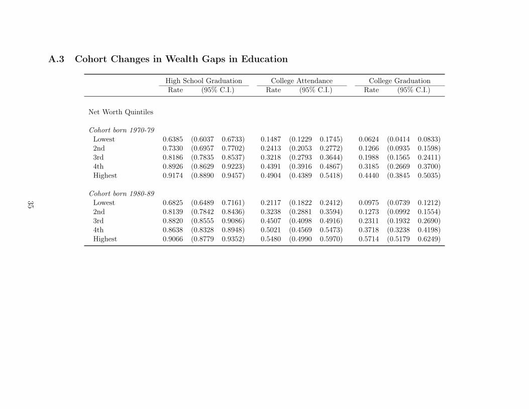
A.3 Cohort Changes in Wealth Gaps in Education

High School Graduation College Attendance College GraduationRate (95% C.I.) Rate (95% C.I.) Rate (95% C.I.)

Net Worth Quintiles

Cohort born 1970-79Lowest 0.6385 (0.6037 0.6733) 0.1487 (0.1229 0.1745) 0.0624 (0.0414 0.0833)2nd 0.7330 (0.6957 0.7702) 0.2413 (0.2053 0.2772) 0.1266 (0.0935 0.1598)3rd 0.8186 (0.7835 0.8537) 0.3218 (0.2793 0.3644) 0.1988 (0.1565 0.2411)4th 0.8926 (0.8629 0.9223) 0.4391 (0.3916 0.4867) 0.3185 (0.2669 0.3700)Highest 0.9174 (0.8890 0.9457) 0.4904 (0.4389 0.5418) 0.4440 (0.3845 0.5035)

Cohort born 1980-89Lowest 0.6825 (0.6489 0.7161) 0.2117 (0.1822 0.2412) 0.0975 (0.0739 0.1212)2nd 0.8139 (0.7842 0.8436) 0.3238 (0.2881 0.3594) 0.1273 (0.0992 0.1554)3rd 0.8820 (0.8555 0.9086) 0.4507 (0.4098 0.4916) 0.2311 (0.1932 0.2690)4th 0.8638 (0.8328 0.8948) 0.5021 (0.4569 0.5473) 0.3718 (0.3238 0.4198)Highest 0.9066 (0.8779 0.9352) 0.5480 (0.4990 0.5970) 0.5714 (0.5179 0.6249)

35