Some matters of great balanceTomas Nilson

Department of Applied Science and DesignMid Sweden University

Doctoral Thesis No. 144Sundsvall, Sweden

2013

MittuniversitetetInstitutionen för tillämpad naturvetenskap och design

ISBN 978-91-87103-67-4 SE-851 70 SundsvallISSN 1652-893X SWEDEN

Akademisk avhandling som med tillstånd av Mittuniversitetet framlägges till of-fentlig granskning för avläggande av filosofie doktorsexamen fredagen den 22mars 2013 i O111, Mittuniversitetet, Holmgatan 10, Sundsvall.

c⃝Tomas Nilson, 2013

Tryck: Tryckeriet Mittuniversitetet

To the Memory of My ParentsTo My ChildrenTo Liu

iv

Abstract

This thesis is based on four papers dealing with two different areas of mathematics.Paper I–III are in combinatorics, while Paper IV is in mathematical physics.

In combinatorics, we work with design theory, one of whose applications aredesigning statistical experiments. Specifically, we are interested in symmetric in-complete block designs (SBIBDs) and triple arrays and also the relationship betweenthese two types of designs.

In Paper I, we investigate when a triple array can be balanced for intersectionwhich in the canonical case is equivalent to the inner design of the correspondingsymmetric balanced incomplete block design (SBIBD) being balanced. For this we de-rive new existence criteria, and in particular we prove that the residual designof the related SBIBD must be quasi-symmetric, and give necessary and sufficientconditions on the intersection numbers. We also address the question of whenthe inner design is balanced with respect to every block of the SBIBD. We showthat such SBIBDs must possess the quasi-3 property, and we answer the existencequestion for all know classes of these designs.

As triple arrays balanced for intersections seem to be very rare, it is natural toask if there are any other families of row-column designs with this property. In Pa-per II we give necessary and sufficient conditions for balanced grids to be balancedfor intersection and prove that all designs in an infinite family of binary pseudo-Youden designs are balanced for intersection.

Existence of triple arrays is an open question. There is one construction of aninfinite, but special family called Paley triple arrays, and one general method forwhich one of the steps is unproved. In Paper III we investigate a third constructionmethod starting from Youden squares. This method was suggested in the literaturea long time ago, but was proven not to work by a counterexample. We show interalia that Youden squares from projective planes can never give a triple array bythis method, but that for every triple array corresponding to a biplane, there is asuitable Youden square for which the method works. Also, we construct the familyof Paley triple arrays by this method.

In mathematical physics we work with solitons, which in nature can be seen asself-reinforcing waves acting like particles, and in mathematics as solutions of cer-tain non-linear differential equations. In Paper IV we study the non-commutativeversion of the two-dimensional Toda lattice for which we construct a family ofsolutions, and derive explicit solution formulas.

keywords: Balanced incomplete block design. Triple array. Balanced grid. Pseudo-Youden design. Youden square. Inner balance. Balanced for intersection. Soliton.Two-dimensional Toda lattice.

v

Sammanfattning

Denna avhandling baseras på fyra artiklar som behandlar två olika områden avmatematiken. Artikel I-III ligger inom kombinatoriken medan artikel IV behandlarmatematisk fysik.

Inom kombinatoriken arbetar vi med designteori som bland annat har tillämp-ningar då man ska utforma statistiska experiment.

I artikel I undersöker vi när en triple array kan vara snittbalanserad vilket i detkanoniska fallet är ekvivalent med den inre designen till den korresponderandesymmetriska balanserade inkompletta blockdesignen (SBIBD) är balanserad. För dettapresenterar vi nya nödvändiga villkor. Speciellt visar vi att den residuala designentill den korresponderande SBIBDen måste vara kvasi-symmetrisk och ger nöd-vändiga och tillräckliga villkor för dess blockskärningstal. Vi adresserar ocksåfrågan om när den inre designen är balanserad med avseende på alla SBIBDensblock. Vi visar att en sådan SBIBD måste ha den egenskap som kallas kvasi-3 ochsvarar på existensfrågan för alla kända klasser av sådana designer.

Eftersom snittbalanserade triple arrays verkar vara väldigt sällsynta är detnaturligt att fråga om det finns andra familjer av rad-kolumn designer som hardenna egenskap. I artikel II ger vi nödvändiga och tillräckliga villkor för att enbalanced grid ska vara snittbalanserad och visar att alla designer i en oändlig familjav binära pseudo-Youden squares är snittbalanserade.

Existensfrågan för triple arrays är öppen fråga. Det finns en konstruktionsme-tod för en oändlig men speciell familj kallad Paley triple arrays och så finns det enallmän metod för vilken ett steg är obevisat. I artikel III undersöker vi en tredjekonstruktionsmetod som utgår från Youden squares. Denna metod föreslogs i lit-teraturen för länge sedan men blev motbevisad med hjälp av ett motexempel. Vivisar bland annat att Youden squares från projektiva plan aldrig kan ge en triplearray med denna metod, men att det för varje triple array som korresponderartill ett biplan, så finns det en lämplig Youden square för vilken metoden fungerar.Vidare konstruerar vi familjen av Paley triple arrays med denna metod.

Inom matematisk fysik arbetar vi med solitoner som man i naturen kan få sesom självförstärkande vågor vilka beter sig som partiklar. Inom matematiken ärde lösningar till vissa ickelinjära differentialekvationer. I artikel IV studerar vi dettvådimensionella Toda-gittret för vilken vi konstruerar en familj av lösningar ochäven explicita lösningsformler.

vi

Acknowledgements

First of all, I would like to express my gratitude to my supervisor Professor Cor-nelia Schiebold. Thank you for always being both inspiring and patient with thisold student. I would also like to thank my assistant supervisors: Egmont Portenfor his support, Lars-Daniel Öhman with whom I hope to do many papers in thefuture and Frank Wikström who was my assistant supervisor in the beginning ofmy doctoral studies.

I thank Jörgen Boo who was very important for me in my early studies andalso my co-author Pia Heidtmann who introduced me to design theory and wasmy Master Thesis supervisor.

To Stefan Borell, Andreas Lind, Sam Lodin, Per Åhag, Abtin Daghighi and Pe-ter Glans. At a small university like Mid Sweden University, your friends and col-leagues become very important. For all discussions, help, inspiration and joyfulmoments, but most of all for your friendship, I thank you.

Finally, thanks Elle, Oskar and Liu for your patience with this young man whoso often loses himself in his work.

vii

viii

Contents

Abstract v

Abstract vi

Acknowledgements vii

List of Papers xi

Notation xvii

1 Entrance 1

1.1 Outline of the thesis . . . . . . . . . . . . . . . . . . . . . . . . . . . . . 1

I Designs 3

2 Block designs 4

2.1 Design theory – a part of combinatorics . . . . . . . . . . . . . . . . . 4

2.2 Balanced incomplete block designs . . . . . . . . . . . . . . . . . . . . 5

2.2.1 Basic definitions and properties . . . . . . . . . . . . . . . . . . 5

2.2.2 When are two designs the same? . . . . . . . . . . . . . . . . . 8

2.3 Symmetric designs and their subdesigns . . . . . . . . . . . . . . . . . 8

2.3.1 Subdesigns and block intersections . . . . . . . . . . . . . . . . 9

2.3.2 Affine and projective planes . . . . . . . . . . . . . . . . . . . . 11

2.3.3 Difference sets . . . . . . . . . . . . . . . . . . . . . . . . . . . . 13

2.3.4 Existence of symmetric designs . . . . . . . . . . . . . . . . . . 15

3 Row-column designs 17

3.1 Definitions and properties . . . . . . . . . . . . . . . . . . . . . . . . . 17

3.1.1 Youden squares . . . . . . . . . . . . . . . . . . . . . . . . . . . 18

3.1.2 Binary pseudo-Youden designs . . . . . . . . . . . . . . . . . . 19

3.1.3 Triple arrays and balanced grids . . . . . . . . . . . . . . . . . 20

3.2 Two construction methods for triple arrays . . . . . . . . . . . . . . . 23

ix

x CONTENTS

3.2.1 Agrawal’s method . . . . . . . . . . . . . . . . . . . . . . . . . 23

3.2.2 Paley triple arrays . . . . . . . . . . . . . . . . . . . . . . . . . 26

4 Research questions and summary of papers I-III 29

4.1 Inner balance? . . . . . . . . . . . . . . . . . . . . . . . . . . . . . . . . 29

4.1.1 Summary of paper I . . . . . . . . . . . . . . . . . . . . . . . . 30

4.2 Any other families? . . . . . . . . . . . . . . . . . . . . . . . . . . . . . 32

4.2.1 Summary of paper II . . . . . . . . . . . . . . . . . . . . . . . . 32

4.3 A third neglected, dismissed and ignored construction . . . . . . . . 33

4.3.1 Summary of paper III . . . . . . . . . . . . . . . . . . . . . . . 33

II Solitons 37

5 Introduction to an operator theoretic approach to soliton theory 38

5.1 Historical background . . . . . . . . . . . . . . . . . . . . . . . . . . . 38

5.2 The operator method . . . . . . . . . . . . . . . . . . . . . . . . . . . . 39

5.3 Illustration of the method for the Korteweg-de Vries equation . . . . 41

5.3.1 The noncommutative Korteweg-de Vries equation and thenoncommutative analogue of its soliton solution . . . . . . . . 41

5.3.2 Derivation of a solution formula for the scalar Korteweg-deVries equation . . . . . . . . . . . . . . . . . . . . . . . . . . . . 42

5.4 N -soliton solutions and nonlinear superposition . . . . . . . . . . . . 45

5.5 Hirota’s bilinear method . . . . . . . . . . . . . . . . . . . . . . . . . . 46

5.6 On traces on operator ideals . . . . . . . . . . . . . . . . . . . . . . . . 50

5.6.1 Spectral traces . . . . . . . . . . . . . . . . . . . . . . . . . . . . 51

5.6.2 Traces for nuclear operators . . . . . . . . . . . . . . . . . . . . 51

5.6.3 Determinants and their relationship to traces . . . . . . . . . . 52

5.7 On elementary operators and Sylvester’s equation . . . . . . . . . . . 52

5.8 Summary of Paper IV . . . . . . . . . . . . . . . . . . . . . . . . . . . . 53

Bibliography 55

List of Papers

This thesis is based on the following papers, herein referred by their Roman nu-merals:

I T. Nilson and P. Heidtmann. Inner balance of symmetric designs. Designs, Codesand Cryptograhy, DOI 10.1007/s10623-012-9730-2.

II T. Nilson. Pseudo-Youden designs balanced for intersection. J. Statist. Plann.Inference, 141, (2011), pp. 2030–2034.

III T. Nilson and L.-D. Öhman. Triple arrays and Youden squares, manuscript.

IV T. Nilson and C. Schiebold. On the noncommutative two-dimensional Toda lattice,manuscript.

Reprints were made with permissions from the publishers.

xi

xii

List of Figures

2.1 A solution of Kirkman’s schoolgirl problem for 15 girls. . . . . . . . . 5

2.2 Three Fano planes. . . . . . . . . . . . . . . . . . . . . . . . . . . . . . 8

2.3 An affine plane of order 3. . . . . . . . . . . . . . . . . . . . . . . . . . 12

2.4 A projective plane of order 3. . . . . . . . . . . . . . . . . . . . . . . . 12

3.1 A latin square of order 4. . . . . . . . . . . . . . . . . . . . . . . . . . . 17

3.2 The underlying design of Potthoff’s experiment. . . . . . . . . . . . . 20

5.1 Simulation of J. S. Russel’s soliton observation. . . . . . . . . . . . . . 39

5.2 The operator method. . . . . . . . . . . . . . . . . . . . . . . . . . . . . 40

5.3 Snapshot of the 1-soliton solution of the Korteweg-de Vries equation. 41

5.4 Two typical interaction patterns for the 2-soliton solution. . . . . . . . 47

5.5 The same 2-soliton solutions as in Figure 5.4 depicted over the xt-plane. . . . . . . . . . . . . . . . . . . . . . . . . . . . . . . . . . . . . . 48

5.6 3-soliton solution shown over the xt-plane. . . . . . . . . . . . . . . . 48

xiii

xiv

List of Tables

3.1 Traffic flow around campus. . . . . . . . . . . . . . . . . . . . . . . . . 20

3.2 The eight types of Paley triple arrays. . . . . . . . . . . . . . . . . . . 27

4.1 The five know classes of quasi-3 designs. . . . . . . . . . . . . . . . . 32

4.2 Twelve types of Youden squares that give Paley triple arrays. . . . . . 35

xv

xvi

Notation

Aut(D) The full automorphism group of a design. DBIBD Balanced incomplete block design.DB The derived design of D with respect to the block. B.DB The residual design of D with respect to the block. B.D′ The complementary design of D.D⋆ The inner design of D.Dτ The dual design of D.GF (q) A finite field of order q.Iv The identity matrix of order v.Jv,b A v × b matrix in which all entries are 1.KdV Korteweg–de Vries equation.KP Kadomtsev–Petviashvili equation.PG(n, q) A n-dimensional projective space over GF (q)

PGd(n, q) An incidence structure formed by the points and the d-dimensionalsubspaces of PG(n, q).

SBIBD Symmetric balanced incomplete block design.

xvii

xviii

Chapter 1

Entrance

Since this thesis treats two different areas, one could ask if they have something incommon. Well, we will see that both areas were started up about the same time,around the year 1840. Another common denominator is balance. In Paper I and II,we search for an inner balance of designs. In Paper IV we study solitons which aresaid to have perfect balance, as the tendencies to disperse and to break cancel eachother out.

1.1 Outline of the thesis

Part I is devoted to design theory. In Chapter 2 we give quite a general introductionto balanced incomplete block designs, although the material is selected to also give afirst background for Paper I-III. In Chapter 3 we introduce row-column designslike Youden squares and triple arrays, and look at construction methods for thelatter ones. In Chapter 4 we declare the research questions for Paper I-III, giveadditional background for these and what results we have achieved.

In Part II we treat soliton theory. After a short historical introduction of thegeneral kind we use most of Chapter 5 to introduce the operator method, and toexemplify it on the Korteweg–de Vries equation. Finally, we give a short summaryof Paper IV.

1

2

Part I

Designs

3

Chapter 2

Block designs

“Never underestimate a theorem that counts something!”John B. Fraleigh. A First Course in Abstract Algebra.

2.1 Design theory – a part of combinatorics

Combinatorial design theory is a branch of mathematics that deals with existence,construction and properties of systems of finite sets whose arrangements satisfycertain concepts like balance or symmetry.

In the past, these structures were studied principally for their aesthetic appeal,but in the early 1900s they came to great practical use when the theory of statisticalexperiments was developed. When statisticians like R. Fisher in the 1920s laid thefoundations of the theory, it was intimately linked to such applications. Then, inthe 1930s, R. C. Bose and his colleagues took it further by developing deep connec-tions with number theory, algebra and finite geometry. Nowadays, design theoryis a field in its own right even if it is still closely connected to applications in statis-tics. But, like most areas of combinatorics, it has been growing fast in the last 30years since the need for discrete structures has increased in the computer age.

The study of block designs can be traced back to 1835 when Plücker [29] in astudy of algebraic curves encountered a design which we now call a Steiner triplesystem, but we will take our starting point a few years later in recreational math-ematics. In the early 1800s the publication Lady’s and Gentlemen’s Diary devotedseveral columns to mathematical problems. One such example is the followingprice question published in 1844 by W. Woolhouse:

“Determine the number of combinations that can be made out of v symbols,each combination having k symbols, with this limitation, that no combinationof t symbols which may appear in any one of them, may appear in any other.”

This problem turned out to be very hard and it is still open, (the existence questionfor Steiner systems1), but T. P. Kirkman [22] solved it completely in the special caseof t = 2 and k = 3, in which he gave necessary and sufficient conditions on v.As a byproduct of this work he then published a more manageable problem in theDiary known as Kirkman’s schoolgirl problem:

1A Steiner system is a (v, k, 1)-BIBD. J. Steiner asked about the existence of (v, 3, 1)-BIBDs in 1853,unaware of Kirkman’s work. As Steiner is more widely known, these systems were named in his honor.

4

2.2 Balanced incomplete block designs 5

“Fifteen young ladies in a school walk out three abreast for seven days in suc-cesion: it is required to arrange them daily so that no two shall walk twiceabreast.”

If the young ladies are numbered 1, 2, . . . , 15, the following arrangement is a solu-tion. Each pair of girls walk together exactly once during the week.

Monday: 1, 6, 11, 2, 7, 12, 3, 8, 13, 4, 9, 14, 5, 10, 15Tuesday: 1, 2, 5, 3, 4, 7, 8, 9, 12, 10, 11, 14, 13, 15, 6Wednesday: 2, 3, 6, 4, 5, 8, 9, 10, 13, 11, 12, 15, 14, 1, 7Thursday: 5, 6, 9, 7, 8, 11, 12, 13, 1, 14, 15, 3, 2, 4, 10Friday: 3, 5, 11, 4, 6, 12, 7, 9, 15, 8, 10, 1, 13, 14, 2Saturday: 5, 7, 13, 6, 8, 14, 9, 11, 2, 10, 12, 3, 15, 1, 4Sunday: 11, 13, 4, 12, 14, 5, 15, 2, 8, 1, 3, 9, 6, 7, 10

Figure 2.1: A solution of Kirkman’s schoolgirl problem for 15 girls.

A first solution was published by A. Cayley, but the problem and especially itsgeneralizations have continued to attract attention.

2.2 Balanced incomplete block designs

In this thesis we deal with properties, existence and construction of these designs.About their usefulness in statistical experiments we confine ourselves to mentionthat statisticians for this consider several types of optimality, and to quote Baileyand Cameron [5] who wrote: “Kiefer’s Theorem asserts that balanced incomplete blockdesigns, if they exist, are optimal in any reasonable sense”.

2.2.1 Basic definitions and properties

The solution of Kirkman’s schoolgirl problem in Figure 2.1 is a special example ofa balanced incomplete block design.

Definition 2.1. A combinatorial design D is a pair (X,B), where X is a set of v ele-ments called points, and B is a collection of b subsets of X called blocks.

1. If there exist positive integers k, r such that each block contains exactly k points andeach point occur in exactly r blocks, then D is called a block design.

2. A block design is called complete if k = v and incomplete if k < v.

3. A block design is balanced if there exists a positive integer λ such that any 2-subsetof X occurs in exactly λ of the blocks. In this case we call λ the index of the design.

We denote a balanced incomplete block design by BIBD and write the parameters (v, b, r, k, λ)or just (v, k, λ), since b and r then will be obtainable. The order of a BIBD is the non-negative integer r − λ. A BIBD where v = b is said to be symmetric (or square) and isdenoted by SBIBD.

In this thesis we mainly use the notion BIBDs but they are also called 2-designsaccording to the following generalization.

6 Block designs

Definition 2.2. Let v, k, λ and t be positive integers such that v > k ≥ t. A t− (v, k, λ)-design is a design (X,B) such that the following properties are satisfied:

1. |X| = v,

2. each block contains exactly k points, and

3. every set of t distinct points is contained in exactly λ blocks.

The general term t-design is used to indicate any t− (v, k, λ)-design.

A block design is often given by a list of its blocks, like the (15, 35, 7, 3, 1)-BIBDin Figure 2.1, but the incidence structure can also be represented by a matrix.

Definition 2.3. The incidence matrix of a block design (X,B) with parameters (v, b, r, k)is a v × b matrix A = [aij ] in which aij = 1 when the ith element of X occurs in the jthblock of B, and aij = 0 otherwise.

Example 2.4. A (6, 10, 5, 3, 2)-BIBD D = (X,B), represented by an incidence matrixin which we have labeled the rows and columns by the elements of X = 1, 2, . . . , 6 andB = B1, B2, . . . , B10 respectively.

A =

B1 B2 B3 B4 B5 B6 B7 B8 B9 B10

1 1 1 1 1 1 0 0 0 0 02 1 1 0 0 0 1 1 1 0 03 0 0 1 1 0 1 1 0 1 04 0 0 1 0 1 1 0 1 0 15 1 0 0 1 0 0 0 1 1 16 0 1 0 0 1 0 1 0 1 1

We will now look at some fundamental properties for BIBDs.

Proposition 2.5. Let D be a block design with parameters (v, b, r, k), then

1. vr = bk.

2. If D is balanced with index λ, then λ(v − 1) = r(k − 1).

That Proposition 2.5 is true can be understood by “double counting” in thematrix A in Example 2.4. Further inspection of A also makes the following resultbelievable.

Theorem 2.6. A (0, 1)-matrix A with v rows and b columns is the incidence matrix of a(v, b, r, k, λ)-BIBD if and only if the following conditions are satisfied.

1. JvA = kJv,b, where 2 ≤ k < v;

2. AAT = (r − λ)Iv + λJv .

where I is the identity matrix and J is the all-one matrix.

In condition (1) of Theorem 2.6 its checked that the block size is constant. Thisbecause there is a related type of designs called pairwise balanced designs, whichsatisfy (2), but have two or more block sizes. The use of incidence matrices openfor notions and tools from linear algebra as in the following examples.

2.2 Balanced incomplete block designs 7

Lemma 2.7. Let A be the incidence matrix of a (v, b, r, k, λ)-BIBD. Then det(AAT ) =(r − λ)v−1rk.

Proposition 2.5 and k < v gives that λ = r(k − 1)/(v − 1) < r, so AAT is non-singular. Further, for a SBIBD we have that A is square and r = k, which togetherwith det(A) = det(AT ) and det(AAT ) = det(A) det(AT ) = (det(A))

2 gives thefollowing corollary.

Corollary 2.8. Let D be a (v, k, λ)-SBIBD and A be an incidence matrix of D. Then A isnon-singular and det(A) = (k − λ)(v−1)/2k.

The following simple but useful result by R. Fisher can be proved by observingthat v = rank(AAT ) ≤ rank(A) ≤ minv, b.

Theorem 2.9. (Fisher’s inequality) For any (v, b, r, k, λ)-BIBD, the number of points doesnot exceed the number of blocks, i.e., v ≤ b.

From a given design it is possible to form new designs.

Definition 2.10. Let D be a combinatorial design. The dual design of D, denoted Dτ isobtained by interchanging the roles of blocks and points.

Fisher’s inequality gives that a necessary condition for the dual design of aBIBD D to also be balanced is that D is a SBIBD, and this condition also turns outto be sufficient.

Theorem 2.11. Let D be a SBIBD. Then the dual design Dτ is also a SBIBD.

Proof. Let A denote the incidence matrix of a (v, k, λ)-SBIBD D. Then Dτ is a block-design with parameters (v, v, k, k) and incidence matrix AT . By Theorem 2.6 Dτ isbalanced if we can show that ATA = (k − µ)Iv + µJv for some positive integer µ.We check (2) of Theorem 2.6. Note that the square matrices here are all of order vand that A is invertible by Corollary 2.8.

AAT = (k − λ)I + λJ

A−1(AAT )A = A−1 ((k − λ)I + λJ)A

ATA = (k − λ)I + λA−1JA,

and as the replication number is equal to the block size k we here have JA = AJwhich gives the result.

There is an important corollary of this result concerning block intersections.

Corollary 2.12. Suppose Bi and Bj are two distinct blocks in a (v, k, λ)-SBIBD. Then|Bi ∩Bj | = λ.

We conlude this first part of the introduction by defining the complementarydesign.

Definition 2.13. Let D = (X,B) be a block design. The complementary design of D,denoted D′, has point set X and the blocks are the sets X \Bi for Bi ∈ B.

Proposition 2.14. Let D be a (v, b, r, k, λ)-BIBD. Then D′ is a(v, b, b− r, v − k, b− 2r + λ)-BIBD, provided that b− 2r + λ > 0.

The condition b − 2r + λ > 0 is not very restrictive as it only excludes BIBDswith v = k + 1.

8 Block designs

2.2.2 When are two designs the same?

If two designs with the same parameters have the “same structure” we say thatthey are isomorphic. For example, there exist 80 non-isomorphic (15, 35, 7, 3, 1)-BIBDs , and among these 80, only seven solve Kirkman’s schoolgirl problem (cf.[14]p. 66).

Definition 2.15. Suppose (X,A) and (Y,B) are two combinatorial designs with |X| =|Y |. Then (X,A) and (Y,B) are isomorphic if there exists a bijection f : X → Y suchthat

[f(x) : x ∈ A : A ∈ A] = B.In other words, if we rename every point x ∈ X by f(x), then the collection of blocks A istransformed into B. The bijection f is called an isomorphism.

An isomorphism from a BIBD D = (X,B) to itself is called an automorphismof D. All automorphisms of D form the full automorphism group of D denoted byAut(D), which is a subgroup of the symmetric group SX , the group of all |X|!permutations of the set X .

(a) D0 = (X,B) (b) D1 = (X,A) (c) D2 = (X,B)

Figure 2.2: Three Fano planes.

Example 2.16. A (7, 3, 1)-SBIBD is sometimes given a graphic representation called theFano plane 2 which can be seen in Figure 2.2. The three SBIBDs given there all have pointset X = 0, 1, 2, 3, 4, 5, 6 and their block sets are listed here below:

D0 = (X,B), B = 0, 1, 2, 0, 3, 4, 0, 5, 6, 1, 3, 5, 1, 4, 6, 2, 3, 6, 2, 4, 5,D1 = (X,A), A = 1, 2, 5, 1, 4, 6, 1, 0, 3, 2, 4, 0, 2, 6, 3, 5, 4, 3, 5, 6, 0,D2 = (X,B), B = 3, 0, 4, 3, 1, 5, 3, 2, 6, 0, 1, 2, 0, 5, 6, 4, 1, 6, 4, 5, 2.

We can define a permutation σ = (0 1 2 5)(3 4 6) on X that transforms the block setB of D0 to the block set A of D1, so σ is an isomorphism and D0 and D1 are isomorphic,but note that A = B so σ is not an automorphism. On the other hand, we can define thepermutation τ = (0 3 1)(2 4 5)(6) on X that transforms the block set of D0 to the blockset of D2. In this case, the block sets are equal so τ is an automorphism.

It can be mentioned that the (7, 3, 1)-SBIBD D is unique up to isomorphism andthat Aut(D) is the projective special linear group PSL(2, 7) of order 168.

2.3 Symmetric designs and their subdesigns

The term “symmetric” is inherited from the early days of the subject and the inci-dence matrix of a SBIBD is seldom symmetric. Some authors use the term square

2The Fano plane is named after Gino Fano (1871–1952) who worked in projective and algebraicgeometry. A (v, k, 1)-SBIBD is a projective plane of order k − 1 as we will see in Section 2.3.2

2.3 Symmetric designs and their subdesigns 9

instead but symmetric is still the most commonly used.

2.3.1 Subdesigns and block intersections

Subdesigns are defined as follows.

Definition 2.17. A block design (Y, C) is a subdesign of a block design (X,B) if andonly if Y ⊆ X and C ⊆ B. The subdesign is proper if Y ⊂ X .

Given a SBIBD we want to construct subdesigns with nice properties, and thefollowing two kinds of substructures are of special interest.

Definition 2.18. Let D = (X,B) be an SBIBD and let B0 ∈ B. The derived design ofD with respect to B0, denoted DB0 , has point set B0 and the blocks are the sets Bi ∩ B0,for Bi ∈ B \ B0.

Proposition 2.19. Let D be a (v, k, λ)-SBIBD and let B be a block of D. Then DB is a(k, v − 1, k − 1, λ, λ− 1)-BIBD, provided that λ ≥ 2.

Definition 2.20. Let D = (X,B) be an SBIBD and let B0 ∈ B. The residual designof D with respect to B0, denoted DB0 , has point set X \ B0 and the blocks are the setsBi \B0, for Bi ∈ B \ B0.

Proposition 2.21. Let D be a (v, k, λ)-SBIBD and let B be a block of D. Then DB is a(v − k, v − 1, k, k − λ, λ)-BIBD.

Example 2.22. An incidence matrix of an (11, 5, 2)-SBIBD where the entries in column0, (block B0), have been emphasized. Rows 0, 1, . . . , 4, and columns 1, 2, . . . , 10, form theincidence matrix of the derived design with respect to the block B0, which is a (5, 10, 1)-BIBD. Rows 5, 6, . . . , 10, and columns 1, 2, . . . , 10, form the incidence matrix of the resid-ual design with respect to B0, which is a (6, 3, 2)-BIBD.

0 1 2 3 4 5 6 7 8 9 100 1 0 0 1 0 0 0 1 1 1 01 1 0 1 0 0 1 0 0 0 1 12 1 1 0 1 0 0 1 0 0 0 13 1 1 1 0 1 0 0 1 0 0 04 1 0 0 0 1 1 1 0 1 0 05 0 1 0 0 1 0 0 0 1 1 16 0 1 1 1 0 1 0 0 1 0 07 0 0 1 1 1 0 1 0 0 1 08 0 0 0 1 1 1 0 1 0 0 19 0 1 0 0 0 1 1 1 0 1 010 0 0 1 0 0 0 1 1 1 0 1

Any (v, b, r, k, λ)-BIBD D with k = r − λ is called a quasi-residual design as ithas the parameters to be a residual design of some SBIBD. If D is a residual ofa (v + r, r, λ)-SBIBD, then it is said to be embeddable. Else, D is said to be non-embeddable.

Remark 2.23. Derived and residual designs can also be defined with respect to a point.Starting with a BIBD D, we define the derived design of D with respect to a point x,denoted Dx, to be what remains when we remove the point x together with all blocks notincident with x. The residual design of D with respect to x is denoted Dx and consistsof the blocks which are not incident with x.

10 Block designs

The theory of block intersections is an area where we have limited knowledge.In Corollary 2.12 we established that any pair of distinct blocks in a (v, k, λ)-SBIBDintersect in λ points, but the picture becomes more unclear when we considerBIBDs with v < b.

Definition 2.24. Suppose D is a block design with blocks B0, B1, . . . , Bb−1. The distinctcardinalities |Bi ∩Bj |, i = j, are called the intersection numbers of D.

Using Fisher’s inequality we can deduce that BIBDs in general have more thanone intersection number.

Proposition 2.25. A (v, b, r, k, λ)-BIBD with v < b has at least two intersection num-bers.

The (6, 10, 5, 3, 2)-BIBD in Example 2.4 has exactly two intersection numbers,|B1 ∩ B2| = 2 and |B2 ∩ B3| = 1. This design belongs to a class of designs whichare relatively well-studied when block intersections are considered.

Definition 2.26. A BIBD with exactly two intersection numbers is called a quasi-symmetric design.

There are many results for special cases of such designs, but the classificationof quasi-symmetric designs is still an open problem. Here, we give one example ofa small, but general result which can be very useful.

Proposition 2.27. ([40], [17]). If x and y, x < y, are the intersection numbers of aquasi-symmetric (v, b, r, k, λ)-BIBD, then y − x divides both k − x and r − λ.

We now turn back to SBIBDs where we will define a property and an extremalclass of these designs according to block intersections. One can say that a SBIBD isregular as any block intersects with itself in k points and doubly regular as any twodistinct blocks intersect in λ points. Thus, we could say that a SBIBD is triply regularif any three distinct blocks intersect in the same number of points. However, thisonly happens in trivial SBIBDs with parameters (v, v − 1, v − 2), and never in anSBIBD D with 2 ≤ k ≤ v−2. This because the dual design Dτ would be a 3-design,which is impossible by the following well-known result.

Lemma 2.28. A t − (v, k, λ) design D = (X,B) with t ≥ 3 and k ≤ v − 2 cannot be asymmetric design.

Proof. Let x ∈ X and let Y be a t−1 subset of X \x. Then Y ∪x is a t-subset ofX . Therefore, there are exactly λ blocks B ∈ B that contain x and contain Y , whichmeans that Dx, the derived design with respect to the point x, is a (t − 1) − (v −1, k − 1, λ) design.

If t ≥ 3, then Dx is a 2-design with v − 1 points. The replication number of D isk so Dx has k ≤ v − 2 blocks, but this cannot be by Fisher’s inequality 2.9.

Therefore, a SBIBD where the cardinality of the intersection of any three dis-tinct blocks just takes on one of two values is called nearly triply regular, or morecommonly quasi-3.

Definition 2.29. An SBIBD D is said to be quasi-3 if there exist integers x and y, calledtriple intersection numbers, such that |A∩B∩C| ∈ x, y for any three distinct blocksA, B, and C of D.

2.3 Symmetric designs and their subdesigns 11

The (11, 5, 2)-SBIBD in Example 2.22 is quasi-3 with triple intersection numbers0 and 1, and we note that these are also the intersection numbers of the deriveddesign with respect to the block B0.

Proposition 2.30. (cf. [19], p. 263) A non-trivial SBIBD D = (X,B) is quasi-3 if andonly if the derived design DB is quasi-symmetric for every B ∈ B.

Sometimes we emphasize that a SBIBD is quasi-3 for blocks. This because thedual definition quasi-3 for points is also used, and this was how quasi-3 designswere first introduced by Cameron [11].

2.3.2 Affine and projective planes

Many designs come from finite geometry and in this section we give an axiomaticdescrition of the two main kinds of finite plane geometry, affine and projectiveplanes, and how they are related to designs.

In Euclidean plane geometry we study the incidence structures formed by pointsand lines in a plane. If there is a unique line trough any two distinct points, and forany point not on a given line, there is a unigue line on the point that is parallel to(i.e., disjoint from) the given line, then an incidence structure with these propertiesis called an affine plane.

Definition 2.31. An affine plane is a pair (X,L), where X is a non-empty set of elementscalled points and L is a family of subsets of X called lines, that satisfy the followingaxioms:

(A1) Any two distinct points lie on a unique line.

(A2) For any line L and any point x = L, there is a unique line M that contains x and isdisjoint from L.

(A3) There exists a triangle, i.e., a set of three points not on a common line.

Two lines with empty intersection are said to be parallel, and this relation be-tween lines is called parallelism. It is an equivalence relation on the lines of an affineplane and the equivalence classes are called parallel classes.

From the axioms of an affine plane it is possible to deduce the following prop-erties.

Theorem 2.32. (cf. [19], p. 63) For any finite affine plane A there is a positive integern ≥ 2 such that every line of A consists of exactly n points, every point lies on exactlyn+ 1 lines, and A has exactly n2 points, n2 + n lines and n+ 1 parallel classes.

We say that such an affine plane is of order n. The smallest affine plane consistsof six lines which are all the 2-subsets of the point set of four points. The affineplane of order 3 is of some historical interest as it was the structure presented byPlücker [29] back in 1835.

Affine planes can be constructed as follows. Let X be a 2-dimensional vectorspace over GF (q), the finite field of order q. For any m, b ∈ GF (q) we call the set(x, y) ∈ X : y = mx + b a line with slope m. For any a ∈ GF (q), we call the set(x, y) ∈ X : x = a a line with infinite slope. If L is the set of all lines, then (X,L)is an affine plane of order q which we denote AG(2, q).

Theorem 2.33. (cf. [19], p. 63) For any prime power q, there exists an affine plane oforder q.

12 Block designs

Figure 2.3: An affine plane of order 3. The three lines 4, 2, 9, 7, 5, 3 and 1, 8, 6 formone of the four parallel classes.

By the properties given in Theorem 2.32 together with axiom (A1) we under-stand that an affine plane is also a BIBD.

Proposition 2.34. (cf. [19], p. 63) An affine plane of order n is an (n2, n, 1)-BIBD, andconversely, for n ≥ 2, any (n2, n, 1)-BIBD is an affine plane of order n.

Affine planes have parallel lines and give us BIBDs with the correspondingproperty. In a projective plane, by contrast, any two lines intersect so parallel linesdo not exist.

Definition 2.35. A projective plane is a pair (X,L) where X is a non-empty set ofelements called points and L is a family of subsets of X called lines, that satisfy thefollowing axioms:

(P1) Any two distinct points lie on a unique line.

(P2) Any two lines have a non-empty intersection.

(P3) There exists an quadrangle, i.e., a set of four points, no three of which lie on acommon line.

Figure 2.4: A projective plane of order 3.

An affine plane can be extended to a projective plane by adding a “line of in-finity” consisting of its parallel classes.

2.3 Symmetric designs and their subdesigns 13

Theorem 2.36. (cf. [19], p. 72) Let A = (X,L) be an affine plane. Let Π be the set ofparallel classes in A. Put X ′ = X ∪ Π. For each line L in A, put L′ = L ∪ π where π isthe parallel class containing L. Finally put L′ = L′ : L ∈ L∪ Π, Then P = (X ′,L′)is a projective plane.

The converse result is also true. Remove any line together with its points froma projective plane and what remains is an affine plane.

Theorem 2.37. (cf. [19], p.73) Let P = (X,L) be a projective plane and let L be a line ofP . Let X ′ = X \ L and L′ = L \ L. Then A = (X ′,L′) is an affine plane.

It follows that a projective plane is a SBIBD. We say that a projective plane P isof order n if each line of P has cardinality n+ 1.

Theorem 2.38. (cf. [19], p. 73) A projective plane of order n is a (n2 + n+ 1, n+ 1, 1)-SBIBD, and conversely, any symmetric (n2 + n + 1, n + 1, 1)-SBIBD with n ≥ 2 is aprojective plane of order n.

We see that there is a projective plane of order n if and only if there is a affineplane of order n.

Theorem 2.39. For any prime power q ≥ 2, there exists a projective plane of order q.

2.3.3 Difference sets

We will now look at an important construction method for SBIBDs.

Let D = (X,B) be a SBIBD. Suppose there is a group G ⊆ Aut(D) acting on ablock B ∈ B such that the orbit of B is all of B, then we immediately get D back.Such a block B is called a base block or a starter block, but a moment of thought givesthat all blocks in the orbit would do as base blocks.

Now we want to start in the other end and use this to construct a SBIBD. Weneed to find a suitable pair of a subset D and a group G such that the action ofG on D gives a SBIBD. We do that by taking the group G as the point set of thedesign and consequently the base block D will be a subset of G. Such base blocksare called difference sets.

Definition 2.40. Let G be a finite group of order v. A k-subset D of G is called a (v, k, λ)-difference set if the multiset

xy−1 : x, y ∈ D,x = y

contains exactly λ copies of every non-identity element of G. Difference sets in abeliangroups are called abelian difference sets and difference sets in cyclic groups are calledcyclic difference sets.

Note that the identity λ(v− 1) = k(k− 1) holds for difference sets as well as forSBIBDs.

Example 2.41. Let G = (Z7,+). Then D = 0, 3, 5, 6 is a (7, 4, 2)-difference set in G.Every non-zero difference occurs exactly two times as a difference between the elements ofD.

It is often possible to find difference sets in groups of type (Zp,+), but there arealso other kinds.

14 Block designs

Example 2.42. There is no (16, 6, 2)-difference set in (Z16,+), yet it is possible to findsuch difference sets in other groups of this order. One non-cyclic but abelian example isD = (0, 2), (1, 0), (1, 1), (1, 3), (2, 2), (3, 2) in the group (Z4 × Z4,+).

A non-abelian example is the group H× Z2 where H = ±1,±i,±j,±k is the quar-ternion group in which the generators satisfy i2 = j2 = k2 = ijk = −1. The setD = (1, 0), (i, 0), (j, 0), (k, 0), (1, 1), (−1, 1) is a non-abelian (16, 6, 2)-difference setin H× Z2.

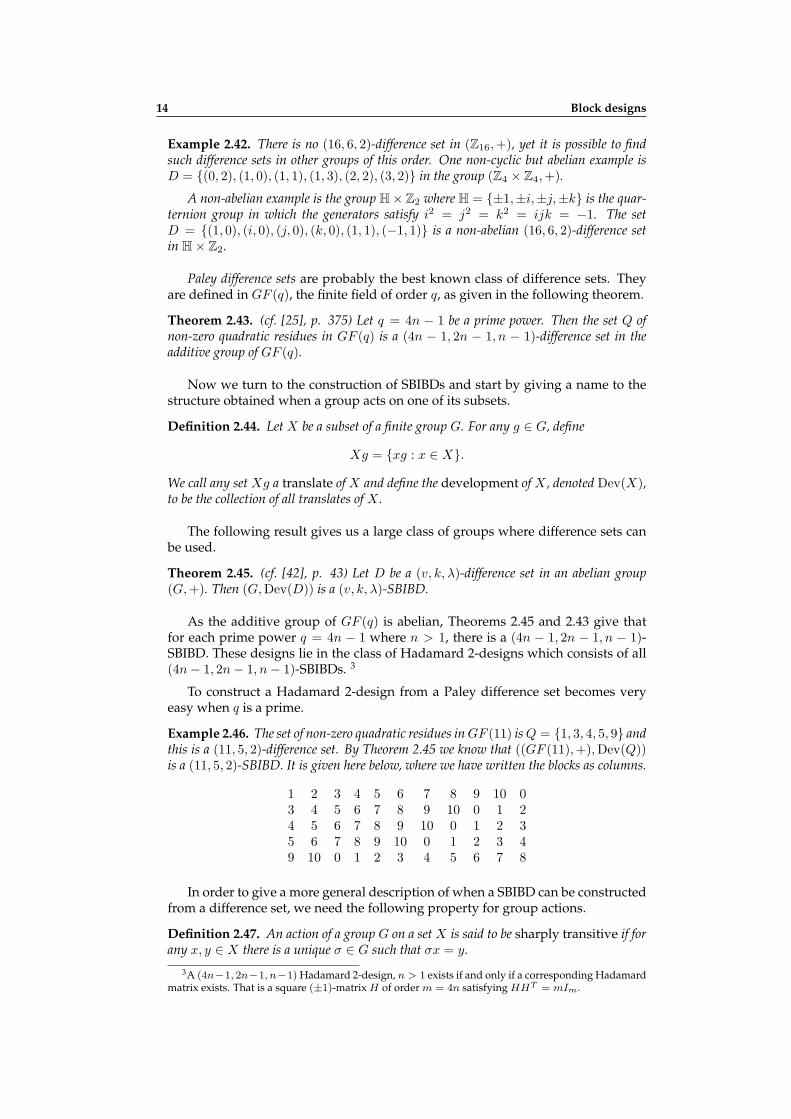
Paley difference sets are probably the best known class of difference sets. Theyare defined in GF (q), the finite field of order q, as given in the following theorem.

Theorem 2.43. (cf. [25], p. 375) Let q = 4n − 1 be a prime power. Then the set Q ofnon-zero quadratic residues in GF (q) is a (4n − 1, 2n − 1, n − 1)-difference set in theadditive group of GF (q).

Now we turn to the construction of SBIBDs and start by giving a name to thestructure obtained when a group acts on one of its subsets.

Definition 2.44. Let X be a subset of a finite group G. For any g ∈ G, define

Xg = xg : x ∈ X.

We call any set Xg a translate of X and define the development of X , denoted Dev(X),to be the collection of all translates of X .

The following result gives us a large class of groups where difference sets canbe used.

Theorem 2.45. (cf. [42], p. 43) Let D be a (v, k, λ)-difference set in an abelian group(G,+). Then (G,Dev(D)) is a (v, k, λ)-SBIBD.

As the additive group of GF (q) is abelian, Theorems 2.45 and 2.43 give thatfor each prime power q = 4n − 1 where n > 1, there is a (4n − 1, 2n − 1, n − 1)-SBIBD. These designs lie in the class of Hadamard 2-designs which consists of all(4n− 1, 2n− 1, n− 1)-SBIBDs. 3

To construct a Hadamard 2-design from a Paley difference set becomes veryeasy when q is a prime.

Example 2.46. The set of non-zero quadratic residues in GF (11) is Q = 1, 3, 4, 5, 9 andthis is a (11, 5, 2)-difference set. By Theorem 2.45 we know that ((GF (11),+),Dev(Q))is a (11, 5, 2)-SBIBD. It is given here below, where we have written the blocks as columns.

1 2 3 4 5 6 7 8 9 10 03 4 5 6 7 8 9 10 0 1 24 5 6 7 8 9 10 0 1 2 35 6 7 8 9 10 0 1 2 3 49 10 0 1 2 3 4 5 6 7 8

In order to give a more general description of when a SBIBD can be constructedfrom a difference set, we need the following property for group actions.

Definition 2.47. An action of a group G on a set X is said to be sharply transitive if forany x, y ∈ X there is a unique σ ∈ G such that σx = y.

3A (4n−1, 2n−1, n−1) Hadamard 2-design, n > 1 exists if and only if a corresponding Hadamardmatrix exists. That is a square (±1)-matrix H of order m = 4n satisfying HHT = mIm.

2.3 Symmetric designs and their subdesigns 15

That a group G acts sharply transitive on a difference set D means that therewill be a single orbit which is necessary for the following generalization of Theo-rem 2.45 for arbitrary finite groups.

Theorem 2.48. (cf. [19], p. 295) A SBIBD D can be obtained as the development ofa difference set in a group G if and only if Aut(D) has a sharply transitive subgroupisomorphic to G.

One example of an application of this theoreom is if we are given that thereexists a (16, 6, 2)-SBIBD D and that (Z4 × Z4,+) ⊆ Aut(D) is sharply transitive.Then Theorem 2.48 gives that there exists a (16, 6, 2)-difference set in (Z4 × Z4,+)from which D can be developed. In this particular case we have already seen sucha difference set in Example 2.42.

It should be mentioned that also some BIBDs with v < b can be constructedvia difference sets, but in such cases we use a set of two or more supplementarydifference sets, also called a difference family.

2.3.4 Existence of symmetric designs

We have already seen that there exists a projective plane, i.e., a (q2+ q+1, q+1, 1)-SBIBD, for each prime power q, and that there exists a Hadamard 2-design, i.e., a(q, (q − 1)/2, (q − 3)/4)-SBIBD, for each prime power q ≡ 3 (mod 4), q ≥ 7. Be-sides these, there are quite a few ingenious constructions of families and specialexamples of SBIBDs (cf, [14], p. 116). But we will focus on the necessary con-ditions given in the “Bruck–Ryser–Chowla Theorem”, the strongest result knowwhen considering existence of these designs.

Theorem 2.49. (Bruck–Ryser–Chowla Theorem). Suppose there exists a symmetric bal-anced incomplete block design with parameters (v, k, λ).

1. If v is even, then k − λ is a perfect square;

2. If v is odd, then there are integers x, y, and z, not all zero, such that

x2 = (k − λ)y2 + (−1)(v−1)/2λz2.

Theorem 2.49 was first proved for (v, k, 1)-SBIBDs, i.e. projective planes, byBruck and Ryser (1949) and then generalized to (v, k, λ)-SBIBDs by Chowla andRyser. The part of the theorem pertaining to even v was first obtained by Schützen-berger [37].

By using the Bruck–Ryser–Chowla Theorem, we can prove non-existence formany SBIBD candidates with parameter sets that satisfy the fundamental identitiesof Proposition 2.5.

Example 2.50. We will prove that there is no (29, 8, 2)-SBIBD. Theorem 2.49 gives thata necessary condition for the existence of such a design is that the following equation has asolution in integers x, y and z, not all zero.

x2 = 6y2 + 2z2 (2.1)

We see that 2|x2 which also means that 2|x. Let x = 2x1 and we can write

2x21 = 3y2 + z2, (2.2)

16 Block designs

which considered modulo 3 becomes 2x1 ≡ z2 (mod 3). As 2 is not a square in Z3,this means that x1 ≡ 0 (mod 3) and consequently z ≡ 0 (mod 3). Let x1 = 3x2 andz = 3z1. Then Equation 2.2 can be written

6x22 = y2 + 3z21 .

We see that also 3|y. Let y = 3y1, then the above equation becomes

2x22 = 3y21 + z21 ,

and we are back in Equation 2.2. As this process can be repeated infinitely often we con-clude that Equation 2.1 has only the trivial solution (x, y, z) = (0, 0, 0), and no (29, 8, 2)-SBIBD exists.

At one time it was even conjectured that the necessary conditions of Theo-rem 2.49, together with those of Proposition 2.5, are sufficient for the existenceof a SBIBD. However, this is not true which became clear when Lam et al. [24]proved that no projective plane of order 10 exists, i.e., no (111, 11, 1)-SBIBD exists,even though the parameters satisfy the conditions of Theorem 2.49. So far, this isthe only example that shows that these conditions are not sufficient.

Among small examples of potential SBIBDs where the parameter sets satisfyTheorem 2.49, but where the existence is undecided is (157, 13, 1), i.e., a projectiveplane of order 12. For biplanes, i.e., (v, k, 2)-SBIBDs, the only values of k for whicha design is known to exist are k = 4, 5, 6, 9, 11, 13, and the smallest biplane forwhich the existence is undecided has parameters (121, 16, 2). For the existence ofSBIBDs with λ > 2 we have a similar situation, which is expressed in the followingconjecture.

Conjecture 2.51. (cf. [14], p. 111) For every λ > 1, there exists only finitely many(v, k, λ)-SBIBDs.

Chapter 3

Row-column designs

3.1 Definitions and properties

Among row-column designs, we are primarily interested in a class called triplearrays but we will also consider some of their predecessors and related designs.

Definition 3.1. A row-column design A is an r × c array in which each cell containsexactly one element of some v-set V of symbols. A is called binary if there is no repetitionin any row or column, and is called equireplicate if every element of V appears the samenumber of times in A.

The prototypical example of a row-column design is a latin square.

Definition 3.2. A latin square L of order n is an n × n array in which each one of nsymbols occurs once in each row and once in each column.

a b c db a d cc d a bd c b a

Figure 3.1: A latin square of order 4.

Latin squares have many applications and are studied intensively. Also, theyare commonly used by a lot of people every day, as the solution of a sudoku puzzleis a latin square.

The main difference between block designs and row-column designs is thatblock designs have two constraints: points and blocks, whereas row-column de-signs have three: rows, columns and symbols. In a latin square, each row is inci-dent with every column, and we say that the constraint rows are orthogonal withrespect to the constraint columns. In fact, any pair of constraints in a latin squareare orthogonal. This explains many of the nice properties of latins squares, butalso that they are “expensive” as designs. There is a need for row-column designswhich are non-orthogonal, but still have nice properties. One such property thatinvolves all three constraints is called adjusted orthogonality.

Definition 3.3. A binary, equireplicate row-column design with replication number k issaid to be adjusted orthogonal if

MNT = kJ,

17

18 Row-column designs

where M and N are the row-symbol and column-symbol incidence matrices of the designand J is the all-one matrix of appropriate order.

Hence, in a row-column design with replication number k, adjusted orthogo-nality means that each pair of a row and a column intersect in k symbols. In exper-iments, one often uses component designs formed by rows-symbols and column-symbols respectively. About relevance of adjusted ortogonaliy for this we quoteJohn and Eccleston [20] who wrote: “If a row-column design has the property of ad-justed orthogonality then one need consider the component designs only.”

3.1.1 Youden squares

Youden’s [44], who did studies on tobacco mosaic virus, realized the need for row-column designs and defined a class based on symmetric designs. Shrikhande [39]explains:

“Sometimes in a design the position within the block is important as a source ofvariation, and the experiment gains in efficiency by eliminating the positionaleffect. The classical example is due to Youden in his studies on tobacco mosaicvirus [44] in 1937. He found that the response to treatments also depends onthe position of the leaf on the plant. If the number of leaves is sufficient so thatevery treatment can be applied to one leaf of a tree, then we get an ordinaryLatin square, in which the trees are columns and the leaves belonging to thesame position constitute the rows. But if the number of treatments is largerthan the number of leaf positions available, then we must have incompletecolumns. Youden used a design in which the columns constituted a balancedincomplete block design, whereas the rows were complete. These designs areknown as Youden squares and can be used when two-way elimination of het-erogeneity is desired.”

Definition 3.4. A Youden square is an arrangement of v symbols in k rows and vcolumns such that

1. every symbol occurs exactly once in each row;

2. the columns form a (v, k, λ)-SBIBD.

Sometimes it is useful to write (2) of Definition 3.4 in the alternative way: “any pairof columns intersects in a constant number of symbols”.

Proposition 3.5. (cf. [19], p. 30) An incidence structure having v points and v blocks,constant block size k, and constant intersection size between any two distinct blocks is a(v, k, λ)-SBIBD.

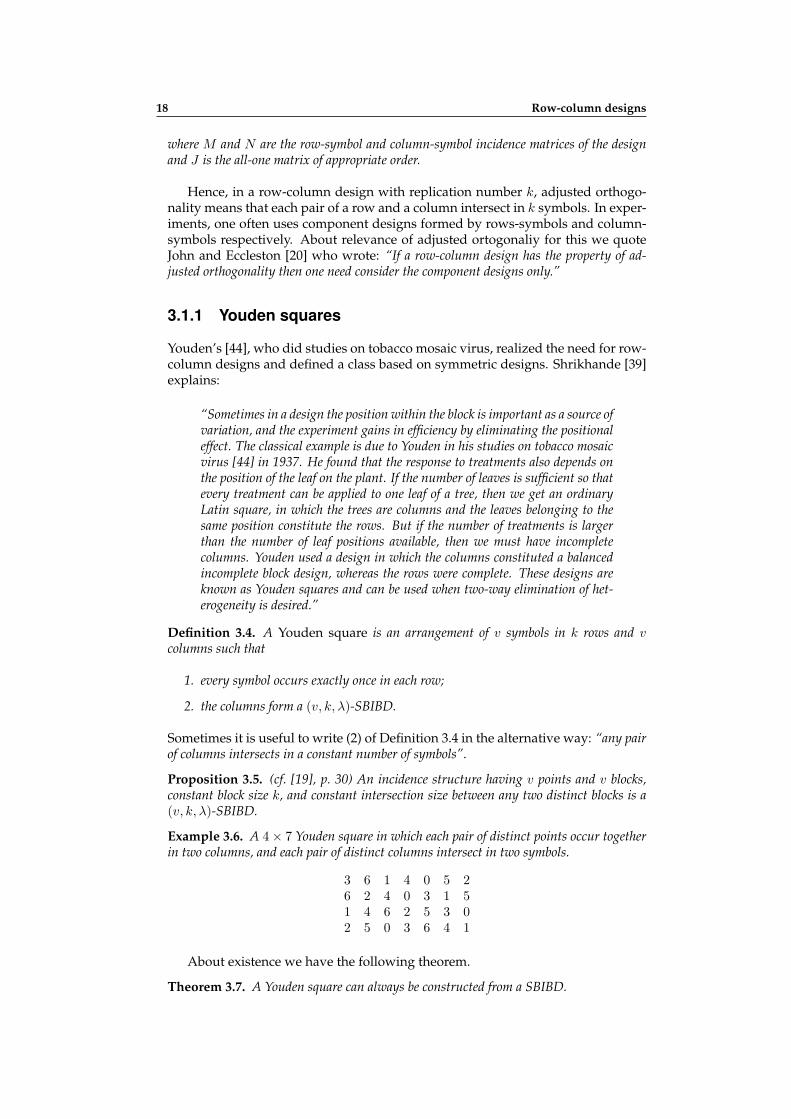
Example 3.6. A 4× 7 Youden square in which each pair of distinct points occur togetherin two columns, and each pair of distinct columns intersect in two symbols.

3 6 1 4 0 5 26 2 4 0 3 1 51 4 6 2 5 3 02 5 0 3 6 4 1

About existence we have the following theorem.

Theorem 3.7. A Youden square can always be constructed from a SBIBD.

3.1 Definitions and properties 19

The above theorem was first proved by Smith and Hartley [41], but we willquote a proof from Raghavarao [35]. This because it uses systems of distinct rep-resentatives (SDRs), and this approach will be of further interest later on. First weremind of the definition and a well-known result for SDRs.

Definition 3.8. Let A1, A2, . . . , An be sets. A system of distinct representatives(SDR) for these sets is an n-tuple (x1, x2, . . . , xn) of elements with the properties

1) xi ∈ Ai, for i = 1, 2, . . . n;

2) xi = xj , for i = j.

Definition 3.9. For any set J ⊆ 1, 2, . . . , n we define

A(J) = ∪j∈JAj .

Theorem 3.10. (P. Hall 1935). A necessary and sufficient condition for the existence ofan SDR for the collection of finite sets A1, A2, . . . , An is that

|A(J)| ≥ |J | for all J ⊆ 1, 2, . . . n.

Proof of Theorem 3.7. Let D be a (v, k, λ)-SBIBD. Write the blocks of D as columnsand note that the replication number r is equal to k by Proposition 2.5. Then anyh columns, 1 ≤ h ≤ v, contain between them hr symbols of which at least h aredistinct as each symbol can occur at most r times in these h columns. Thus, byTheorem 3.10, an SDR exists for the v columns, and this SDR will be a permutationof the v symbols of D. Bring this SDR to the first row. Deleting the first row wefind that each column now contains r− 1 symbols, and h of these columns containh(r − 1) symbols of which at least h are distinct. Hence another SDR exists for thecolumns, and we bring this SDR to the second row. Continuing similarly, we canprove that the k rows can be so arranged that every symbol occurs exactly once ineach row.

Remark 3.11. A Youden square is obviously not a square array and some authors use thename Youden rectangle instead. However, the reason for the term square is said to be theuse of another representation with a v×v array, each of whose entries is either blank or oneof k symbols, each symbol occurring exactly once in each row and in each column, everypair of rows (or columns) being occupied simultaneously in λ columns (or rows).

3.1.2 Binary pseudo-Youden designs

The usual latin square and Youden square designs have been generalized to giveother types of designs. A binary example is the following class.

Definition 3.12. A binary row-column design where the rows and columns together forma BIBD is called a binary pseudo-Youden design.

As a block design is formed, we know that the number of rows are equal to thenumber of columns. We denote such an r × r binary pseudo-Youden design on velements by PY D(v : r × r).

Example 3.13. A binary PY D(9 : 6 × 6). The rows and columns together form a(9, 12, 8, 6, 5)-BIBD.

1 2 3 4 5 67 8 9 1 2 35 4 7 9 6 88 1 2 5 7 46 9 4 3 1 73 6 5 8 9 2

20 Row-column designs

The class was named by Cheng [12], but the small PY D(9 : 6×6) has been usedand studied since the 1950s, by Kshirsagar [23], Preece [32] and others. McSorleyand Phillips [28] gave a complete enumeration of it and found that there are 696non-isomorphic PY D(9 : 6× 6).1

By combining the structures of Youden squares and affine planes, Cheng [13]was able to prove the existence of an infinite family of PYDs.

Theorem 3.14. ([13]). Let s be a prime or a prime power with s ≡ 3 (mod 4). Thenthere exists a binary pseudo-Youden design with v = s2 and r = s(s+1)

2 .

Taking s = 3 in Theorem 3.14 gives a PY D(9 : 6 × 6) which is the smallestmember in this family, and to the best of our knowledge, all binary PY D(v : r× r)belong to this family.

3.1.3 Triple arrays and balanced grids

In the 1960s Agrawal [2] amongst others, started to construct some row-columndesigns for two-way elimination of heterogenity that we now call triple arrays. Inthese designs, strong properties co-exist as two BIBDs are merged together in sucha way that the design is adjusted orthogonal. We will look at the earliest examplewe have seen, an application example by Potthoff [30]. Note that this experimentwas not made for its own sake, but purely to present the design and to illustratethe analysis part.

Example 3.15. The experiment is to measure traffic flow at 10 different points aroundthe campus in the mornings. The observations were made every 10 minutes between 8a.m. and 9 a.m. on 5 mornings in september 1961. A given observation consisted ofcounting the number of vehicles passing the specified point during a 5-minute period. Theraw results of the experiment are given in the following table. For example, 72 vehiclespassed location (1) Monday between 8.00 and 8.05. A complete experiment would consist

Days 8.00 8.10 8.20 8.30 8.40 8.50Monday 72(1) 101(6) 59(3) 53(4) 10(8) 78(10)Tuesday 49(2) 50(1) 98(9) 92(10) 38(5) 12(8)Wednesday 62(3) 13(8) 49(7) 50(2) 73(9) 54(4)Thursday 52(4) 35(7) 89(1) 82(9) 46(6) 67(5)Friday 57(5) 55(2) 100(10) 46(6) 34(3) 48(7)

Table 3.1: Traffic flow around campus.

of 300 observations, but Potthoff used a design constructed in such a way that only 30observations were required for the analysis. Let us look at the bare design.

1 6 3 4 8 102 1 9 10 5 83 8 7 2 9 44 7 1 9 6 55 2 10 6 3 7

Figure 3.2: The underlying design of Potthoff’s experiment on traffic flow.

1Two binary PYDs A1 and A2 on the same set of symbols are isomorphic if A2 can be obtained fromA1 by a permutation of its symbols, rows or columns.

3.1 Definitions and properties 21

This is a triple array. We will see that both rows and columns as sets constitutesduals of balanced incomplete block designs, merged so that every row-column pairintersects in a constant number of symbols.

Definition 3.16. Let A be a binary r × c row-column design on v symbols, equireplicatewith replication number k, where k < r, c, and let λrr, λcc and λrc be positive integers. IfA satisfies that

1. any two distinct rows intersect in λrr symbols;

2. any two distinct columns intersect in λcc symbols;

3. any row and column intersect in λrc symbols;

then A is called a triple array, denoted by TA(v, k, λrr, λcc, λrc : r×c). An array as abovethat satisfies conditions 1–2 is called a double array and is denoted by DA(v, k, λrr, λcc :r × c).

Note that property (3) in Definition 3.16 means that A is adjusted orthogonal.Also, properties (1) and (2) in this context give dual conditions for BIBDs, so wehave two equivalent definitions at our disposal.

Definition 3.17. Let A be an r × c row-column design on v symbols that satisfies

1. the rows are the dual of a BIBD,

2. the columns are the dual of a BIBD,

3. every row intersects every column in a constant number of symbols,

then A is called a triple array.

Similar to Fisher’s inequality 2.9 for BIBDs, there is a useful inequality for triplearrays.

Theorem 3.18. ([4][26]) Any triple array TA(v, k, λrr, λcc, λrc : r × c) satisfies,

v ≥ r + c− 1.

The triple array we saw in Example 3.15 lies in the extremal case where v =r+c−1. Also, Agrawal [2] worked and suggested a construction method for triplearrays in this case, starting from SBIBDs. We will look at this construction methodin Section 3.2 but first we will consider the opposite direction, and for this we usethe following observation.

Lemma 3.19. ([26]) Suppose A is a TA(v, k, λrr, λcc, λrc : r × c) with v = r + c − 1.Then

λcc = r − λrc = v − 2c+ λrr + 1.

Theorem 3.20. ([26]) Suppose A is a TA(v, k, λrr, λcc, λrc : r × c) with v = r + c− 1.Then there exists a (v + 1, r, λcc)-SBIBD.

Proof. Label the rows of A by i = 1, 2, . . . , r, the columns by j = r+1, r+2, . . . , r+c,and let Ri and Cj denote the support of row i and column j respectively. Weconstruct a (v + 1, r, λcc)-SBIBD D = (X,B) by taking these labels as point set, soX = 1, 2, . . . , r + c, and we construct one block for each symbol s of A by:

Bs = i : s ∈ Ri ∪ j : s ∈ Cj for s = 1, 2, . . . , v,

22 Row-column designs

and also add the blockB0 = 1, 2, . . . , r.

We note that |X| = |B| = v + 1 and that the block size of D is constant as anygiven s does not occur in r − k rows but does occur in k columns of A, so |Bs| =(r − k) + k = r = |B0|. D is equireplicate because any point i will be in a Bs whens does not occur in Ri. This happens in v − c cases and in the block B0, so i willbe in v − c + 1 = r blocks. Also, a point j occurs in different Bs for each of the rsymbols in Cj . It remains to show that D is balanced and we have three cases ofpairs of points.

i1, i2 : Given any two distinct rows i1 and i2 of A, the sieve principle gives that|(Ri1 ∪Ri2)

| = v−2c+λrr. As the pair i1, i2 also occurs in B0, it will be in a totalof v − 2c+ λrr + 1 blocks of D, and Lemma 3.19 gives that v − 2c+ λrr + 1 = λcc.

j1, j2 : A pair j1, j2 will meet in λcc blocks of D as |Cj1 ∩ Cj2 | = λcc.

i, j : A pair i, j will meet in |Ri ∩ Cj | = r − λrc blocks of D, and Lemma 3.19

gives that r − λrc = λcc.

The component designs of the triple array correspond to subdesigns of the con-structed SBIBD which was pointed out by [27].

Corollary 3.21. Let A be a triple array with v = r + c − 1 and let D be the SBIBDconstructed from A as in Theorem 3.20. Then

1. the dual design of the rows in A is the complementary design of the derived designof D with respect to B0,

2. the dual design of the columns in A is the residual design of D with respect to B0.

The converse of Theorem 3.20 is open, and is known as Agrawal’s Conjecture.

Conjecture 3.22. ([2]). If there exists a (v+1, r, λcc)-SBIBD with r−λcc > 2 then thereexists a TA(v, k, λrr, λcc, k : r × c) with v = r + c− 1.

When we examine construction methods in Section 3.2, we will take a closer lookat Agrawal’s Conjecture and we will also see that there are many triple arrays withv = r + c− 1. However, when v > r + c− 1, there is only one know triple array. Itis a TA(35, 3, 5, 1, 3 : 7× 15) that was asked for by Preece [31] already in 1976, butwas found much later by McSorley et al. [26] and whose structure was studied byYucas [45].

We now turn our attention to a class of designs which is quite unknown, butin fact contains almost every row-column design mentioned in this thesis. Theyare called balanced grids and were introduced by McSorley et al. [26] in 2005. Inbalanced grids we consider how pairs of distinct symbols occur together. Let xand y be two symbols in a binary row-column design. Let rxy denote the numberof rows where both x and y occur and cxy the number of columns where both xand y occur.

Definition 3.23. Let A be a binary row-column design and define µxy = rxy + cxy . Ifthere is a constant µ such that µxy = µ for every distinct x and y, then A will be called abalanced grid.

Theorem 3.24. ([26]). An r × c balanced grid based on v symbols satisfies

µ =rc(r + c− 2)

v(v − 1),

3.2 Two construction methods for triple arrays 23

moreover, it will be equireplicate, with replication number

k =rc

v.

A balanced grid is denoted by BG(v, k, µ : r × c).

There is an inequality also for balanced grids.

Theorem 3.25. ([26]) Any balanced grid BG(v, k, µ : r × c) satisfies v ≤ r + c− 1.

That the inequalities for triple arrays and balance grids are both extremal whenv = r + c− 1 suggest the following result.

Theorem 3.26. ([27]) Let v = r+ c− 1. Then every triple array is a TA(v, k, c− k, r−k, k : r × c) and every balanced grid is a BG(v, k, k : r × c), and they are equivalent.

This theorem is useful as it gives us an alternative view and definition of triplearrays in the canonical case. But let us remember that besides these triple arrays,also latin squares, Youden squares and, as was pointed out in [28], pseudo-Youdendesigns all are balanced grids.

3.2 Two construction methods for triple arrays

Quite a few triple arrays are known. A comprehensive list of these and manyexamples can be found in [26], and there is also a database [46] from which triplearrays can be downloaded. However, the existence question is still open. What wehave is a general construction for the canonical case v = r + c− 1 called Agrawal’smethod. This method would give all such triple arrays, but one of the steps of theconstruction is unproved and is left to trial and error solutions. Besides Agrawal’smethod, we have the family of Paley triple arrays, which is the single known infinitefamily of triple arrays. In the non-extremal case when v > r+ c− 1, the only triplearray known is the TA(35, 3, 5, 1, 3 : 7× 15) in [26] as we have mentioned before.

3.2.1 Agrawal’s method

In 1966, Agrawal [2] gave a construction method for triple arrays starting from(v+1, r, λcc)-SBIBDs. He could not prove the method, although he found no coun-terexample provided that r − λcc > 2.

Given a (v, k, λ)-SBIBD D and a block B of D we know by Proposition 2.21 thatthe residual design DB is a (v−k, v−1, k, k−λ, λ)-BIBD, and the following lemmagives us a simular result for the complementary design of the derived design DB ,provided that D is non-trivial.

Lemma 3.27. Let D = (X,B) be a (v, k, λ)-SBIBD with v − 1 > k. Then (DB)′, the

complementary design of the derived design of D with respect to some block B ∈ B, is a(k, v − 1, v − k, k − λ, v − 2k + λ)-BIBD.

Proof. A moment of thought gives the four first parameters of (DB)′, and the sieve

principle gives that its index must be v − 2k + λ. So what we need to prove is thatv − 2k + λ > 0. Let x, y ∈ X . As 2k − λ is the number of blocks that contain one orboth of x and y, we cannot have v−2k+λ < 0. So let us assume that v−2k+λ = 0,

24 Row-column designs

and we will show that this can only happen if v = k+ 1. We use Proposition 2.5 todevelop

v − 2k + λ =λ(v − 1)(v − 2k)

k(k − 1)+

λk(k − 1)

k(k − 1)=

λ(v2 − 2vk − v + 2k + k2 − k)

k(k − 1)=

=λ((v − k)2 − (v − k)

)k(k − 1)

=λ(v − k)(v − k − 1)

k(k − 1),

which is equal to 0 if and only if v = k + 1.

These two BIBDs seem to have promising parameters for being merged to-gether as they have the same number of blocks, same block size and mirror eachother when it comes to the number of points and replication number. Further,Agrawal [1] had made the following observation.

Lemma 3.28. ([1]) Let D be a (v, k, λ)-SBIBD. Let N1 denote the incidence matrix of theresidual design of D with respect to a block B, and let N2 denote the incidence matrix of thecomplementary design of the derived design of D with respect to the same block B. Then

N1NT2 = (k − λ)Jv−k,k,

where J is an (v − k)× k all-one matrix.

A comparison of this result with Definition 3.3 suggests that it might be possi-ble to merge this pair of BIBDs into a row-column design with adjusted orthogo-nality.

Construction 3.29. Agrawal’s method [2].

1. Take a (v + 1, r, λcc)-SBIBD with r − λcc > 2 and label the blocks B0, B1, . . . , Bv.

2. Denote the blocks of the residual design DB0 by B′s = Bs \B0, s = 1, 2, . . . , v, and

label its elements j = 1, 2, . . . , c, where c = v + 1− r.

3. Let N2 denote the incidence matrix of the complement of the derived design DB0

with blocks B′′s = B0 \Bs, s = 1, 2, . . . , v, and elements labeled i = 1, 2, . . . , r.

4. For each column s = 1, 2, . . . , v, of N2, replace the entries 1 by the elements of theblock B′

s in any order, and let the remaining cells be undefined.

5. Rearrange the elements within each column s, using only the defined cells, so thateach element of DB0 occurs exactly once in every row. Then we have an r × v arrayA where A(i, s) = j in rc defined cells, (A is called the RL-form of the triple array).

6. Map the defined triplets (i, s, j) from A to the r×c array C where C(i, j) = s. ThenC is a r × c triple array.

Note that it is not proven that the rearranging step (5) of Agrawal’s method canalways be done. Ragesvarao and Nageswararao [36] claimed that they had provenit, using an argument with systems of distinct representatives, similary to the prooffor Youden squares in Theorem 3.7. But this proof is flawed, as was pointed out byWallis and Yucas [43].

We will write out a proof of Agrawal’s method where we assume that the re-arrangment step (5) can be carried out. But first we use Lemma 3.27 and Propo-sition 2.21 to simplify the parameter expressions of DB and the complementarydesign of DB of a (v + 1, r, λcc)-SBIBD.

3.2 Two construction methods for triple arrays 25

Lemma 3.30. Let D be a (v + 1, r, λcc)-SBIBD and let B be a block of D. If we writec = v + 1− r, k = r − λcc and λrr = v − 2r + λcc + 1, then the complementary designof DB is a (r, v, c, k, λrr)-BIBD, and DB is a (c, v, r, k, λcc)-BIBD.

Proposition 3.31. (For Agrawal’s method) Let D be a (v+1, r, λcc)-SBIBD with r−λcc >2 and assume that the rearranging step (5) of Construction 3.29 can always be carried out.Then the array C of Construction 3.29 is a triple array.

Proof. Suppose it is possible to rearrange the elements as specified in step (5) ofConstruction 3.29. The r × v array A has rc defined cells which means that C isan r × c row-column design with v symbols. C is equireplicate with replicationnumber r − λcc as each block B′′

s has r − λcc elements. That C is binary followsfrom the rearranging step (5).

N2 is the incidence matrix for points and blocks of the complementary designof DB0 . When we replace the entries 1 in step (4) and rearrange in (5), it does notaffect what rows and columns are incident. So after the transcription to C, whencolumns and symbols are interchanced, N2 will serve as incidence matrix for rows–symbols in C. Similary, N1 is the incidence matrix for points and blocks of DB0 .Moving these points (symbols) within columns to N2 does not affect what points(symbols) and columns are incident. Thus, N1 is the incident matrix for symbols–columns in A and after the transcription to C, N1 will serve as the incident matrixfor columns–symbols in C.

By Lemma 3.30, N2 is the incidence matrix of a (r, v, c, k, λrr)-BIBD and N1

is the incidence matrix of a (c, v, r, k, λcc)-BIBD, so both rows and columns formduals of BIBDs respectively. Hence, C is a double array.

Let M(rs) and M(cs) be incidence matrices for rows-symbols and columns-symbolsof C respectively, then by Lemma 3.28

M(cs)MT(rc) = N1N

T2 = (r − λcc)Jc,r.

Hence, C is adjusted orthogonal so C is a triple array.

Example 3.32. Let us construct a 5 × 6 triple array by Agrawal’s method. We startwith a (11, 5, 2)-SBIBD D, here given by its incidence matrix N . We have labeled theblocks/columns, and to make it more easy to see the structure we have written N so thatB0 consists of the first five elements, emphasized the 1’s in that column and used the sign(−) instead of the entry (0).

N =

0 1 2 3 4 5 6 7 8 9 101 − − 1 − − − 1 1 1 −1 − 1 − − 1 − − − 1 11 1 − 1 − − 1 − − − 11 1 1 − 1 − − 1 − − −1 − − − 1 1 1 − 1 − −− 1 − − 1 − − − 1 1 1− 1 1 1 − 1 − − 1 − −− − 1 1 1 − 1 − − 1 −− − − 1 1 1 − 1 − − 1− 1 − − − 1 1 1 − 1 −− − 1 − − − 1 1 1 − 1

Let N1 denote the incidence matrix for the residual design DB0 . It is a (6, 3, 2)-BIBDand we label the elements j = 1, 2, . . . , 6. Let N2 denote the incidence matrix for the

26 Row-column designs

complement of the derived design DB0 . It is a (5, 3, 3) BIBD and we label the elementsi = 1, 2, . . . , 5.

Let the elements j from block B′s of DB0 replace the 1’s in column s of N2 for every

s = 1, 2, . . . , v.

1 2 3 4 5 6 7 8 9 101 1 6 1 2 6 62 5 2 3 3 5 23 3 4 5 6 6 54 4 4 5 1 3 45 2 2 3 4 1 1

Rearrange the elements within columns so that every element occurs exactly once in everyrow. Then we have the array A where A(i, s) = j, (the RL-form of the triple array).

A =

1 2 3 4 5 6 7 8 9 101 5 6 1 2 3 42 1 3 4 6 5 23 2 3 5 4 6 14 2 4 5 1 3 65 2 3 4 6 5 1

Construct the array C by C(i, j) = s. It is a TA(10, 3, 3, 2, 3 : 5× 6).

C =

1 2 3 4 5 61 4 5 6 10 1 22 1 8 3 4 7 63 9 2 4 7 5 84 8 3 9 5 6 105 10 1 2 3 9 7

Agrawal [2] wrote that his method did not seem to work when starting with a(v, k, λ)-SBIBD in which k − λ ≤ 2. However, the condition k − λ > 2 does notexclude any triple array that can be constructed in any other way.

Observation 3.33. A (v, k, λ)-SBIBD with k − λ = 2 is either a (7, 3, 1)-SBIBD or itscomplementary design, a (7, 4, 2)-SBIBD.

Proof. As k− λ = 1 implies the trivial case k = v − 1 we assume that k− λ = 2. ByProposition 2.5 we can write (k − 2)(v − 1) = k(k − 1). So, k − 2 divides k(k − 1)and long division gives

v − 1 = k + 1 +2

k − 2.

Hence, k can only take values in 3, 4 which in both cases give v = 7.

These SBIBDs would correspond to a TA(6, 2, 2, 1, 2 : 3× 4) which is known tonot exist by exhaustion.

3.2.2 Paley triple arrays

“God loves odd numbers.”Vergilius, Eclogae

3.2 Two construction methods for triple arrays 27

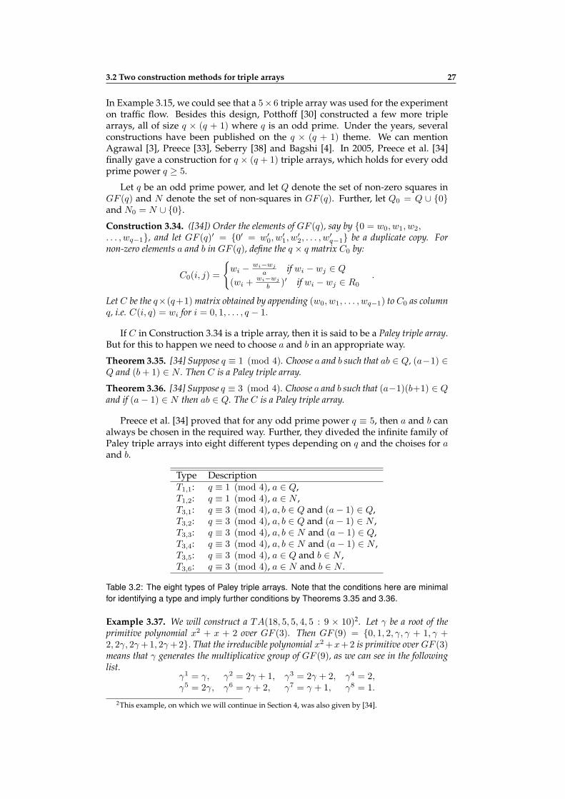
In Example 3.15, we could see that a 5× 6 triple array was used for the experimenton traffic flow. Besides this design, Potthoff [30] constructed a few more triplearrays, all of size q × (q + 1) where q is an odd prime. Under the years, severalconstructions have been published on the q × (q + 1) theme. We can mentionAgrawal [3], Preece [33], Seberry [38] and Bagshi [4]. In 2005, Preece et al. [34]finally gave a construction for q × (q + 1) triple arrays, which holds for every oddprime power q ≥ 5.

Let q be an odd prime power, and let Q denote the set of non-zero squares inGF (q) and N denote the set of non-squares in GF (q). Further, let Q0 = Q ∪ 0and N0 = N ∪ 0.

Construction 3.34. ([34]) Order the elements of GF (q), say by 0 = w0, w1, w2,. . . , wq−1, and let GF (q)′ = 0′ = w′

0, w′1, w

′2, . . . , w

′q−1 be a duplicate copy. For

non-zero elements a and b in GF (q), define the q × q matrix C0 by:

C0(i, j) =

wi − wi−wj

a if wi − wj ∈ Q

(wi +wi−wj

b )′ if wi − wj ∈ R0

.

Let C be the q×(q+1) matrix obtained by appending (w0, w1, . . . , wq−1) to C0 as columnq, i.e. C(i, q) = wi for i = 0, 1, . . . , q − 1.

If C in Construction 3.34 is a triple array, then it is said to be a Paley triple array.But for this to happen we need to choose a and b in an appropriate way.

Theorem 3.35. [34] Suppose q ≡ 1 (mod 4). Choose a and b such that ab ∈ Q, (a−1) ∈Q and (b+ 1) ∈ N . Then C is a Paley triple array.

Theorem 3.36. [34] Suppose q ≡ 3 (mod 4). Choose a and b such that (a−1)(b+1) ∈ Qand if (a− 1) ∈ N then ab ∈ Q. The C is a Paley triple array.

Preece et al. [34] proved that for any odd prime power q ≡ 5, then a and b canalways be chosen in the required way. Further, they diveded the infinite family ofPaley triple arrays into eight different types depending on q and the choises for aand b.

Type DescriptionT1,1: q ≡ 1 (mod 4), a ∈ Q,T1,2: q ≡ 1 (mod 4), a ∈ N ,T3,1: q ≡ 3 (mod 4), a, b ∈ Q and (a− 1) ∈ Q,T3,2: q ≡ 3 (mod 4), a, b ∈ Q and (a− 1) ∈ N ,T3,3: q ≡ 3 (mod 4), a, b ∈ N and (a− 1) ∈ Q,T3,4: q ≡ 3 (mod 4), a, b ∈ N and (a− 1) ∈ N ,T3,5: q ≡ 3 (mod 4), a ∈ Q and b ∈ N ,T3,6: q ≡ 3 (mod 4), a ∈ N and b ∈ N .

Table 3.2: The eight types of Paley triple arrays. Note that the conditions here are minimalfor identifying a type and imply further conditions by Theorems 3.35 and 3.36.

Example 3.37. We will construct a TA(18, 5, 5, 4, 5 : 9 × 10)2. Let γ be a root of theprimitive polynomial x2 + x + 2 over GF (3). Then GF (9) = 0, 1, 2, γ, γ + 1, γ +2, 2γ, 2γ+1, 2γ+2. That the irreducible polynomial x2+x+2 is primitive over GF (3)means that γ generates the multiplicative group of GF (9), as we can see in the followinglist.

γ1 = γ, γ2 = 2γ + 1, γ3 = 2γ + 2, γ4 = 2,γ5 = 2γ, γ6 = γ + 2, γ7 = γ + 1, γ8 = 1.

2This example, on which we will continue in Section 4, was also given by [34].

28 Row-column designs

Take a = γ4 and b = γ6. Then ab = γ2 ∈ Q, (a − 1) = γ8 ∈ Q and (b + 1) = γ ∈N0. Theorem 3.35 gives that these choices will give a Paley triple array of type T1,1 inConstruction 3.34.

First we order GF (9) by 0, γ, γ2, . . . , γ8 and note that a−1 = γ4 and b−1 = γ2.Then, we compute the entries in C0, let us do C0(5, 1) as an example. As γ5−γ = γ ∈ N0

we have that

C0(5, 1) =(γ5 + (γ5 − γ)γ2

)′= (γ5 + γ3)′ = (γ + 2)′ = γ6′ .

When all entries in C0 are in place, we append (0, γ, γ2, . . . , γ8) as column 9 to get thePaley triple array C.

C =

0′ γ7′ γ6 γ′ γ8 γ3′ γ2 γ5′ γ4 0

γ4′ γ′ 0′ γ8 γ5′ γ2′ γ7 γ6 γ3 γ

γ6 γ8′ γ2′ γ5 γ7′ γ3 0 γ′ γ4′ γ2

γ6′ γ8 γ5 γ3′ 0′ γ2 γ7′ γ4′ γ γ3

γ8 γ3′ γ6′ γ2′ γ4′ γ7 γ′ γ5 0 γ4

γ8′ γ6′ γ3 γ2 γ7 γ5′ 0′ γ4 γ′ γ5

γ2 γ7 0 γ5′ γ8′ γ4′ γ6′ γ γ3′ γ6

γ2′ γ6 γ3′ γ8′ γ5 γ4 γ γ7′ 0′ γ7

γ4 γ3 γ5′ γ 0 γ7′ γ2′ γ6′ γ8′ γ8

To construct C in Example 3.37 requires a lot of computations. However, when

q is a prime we just have to compute one column (or row) of C0, and then it is veryeasy to complete the array.

Proposition 3.38. ([34]) If q is a prime and GF (q) is ordered by 0, 1, 2, . . . , q− 1 thenC0 has cyclic transversals. That is

C0(i+ k, j + k) = C(i, j) + k,

where row and column numbers are interpreted as integers modulo q, when additions areinvolved.

Chapter 4

Research questions andsummary of papers I-III

In this chapter, we discuss the issues that formed the basis for our research andprovide additional background on these. Furthermore, we describe how we ap-proached these problems and what results we achieved.

4.1 Inner balance?

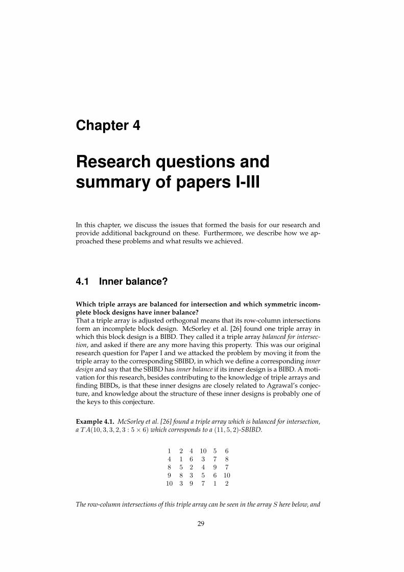
Which triple arrays are balanced for intersection and which symmetric incom-plete block designs have inner balance?That a triple array is adjusted orthogonal means that its row-column intersectionsform an incomplete block design. McSorley et al. [26] found one triple array inwhich this block design is a BIBD. They called it a triple array balanced for intersec-tion, and asked if there are any more having this property. This was our originalresearch question for Paper I and we attacked the problem by moving it from thetriple array to the corresponding SBIBD, in which we define a corresponding innerdesign and say that the SBIBD has inner balance if its inner design is a BIBD. A moti-vation for this research, besides contributing to the knowledge of triple arrays andfinding BIBDs, is that these inner designs are closely related to Agrawal’s conjec-ture, and knowledge about the structure of these inner designs is probably one ofthe keys to this conjecture.

Example 4.1. McSorley et al. [26] found a triple array which is balanced for intersection,a TA(10, 3, 3, 2, 3 : 5× 6) which corresponds to a (11, 5, 2)-SBIBD.

1 2 4 10 5 64 1 6 3 7 88 5 2 4 9 79 8 3 5 6 1010 3 9 7 1 2

The row-column intersections of this triple array can be seen in the array S here below, and

29

30 Research questions and summary of papers I-III

they form a (10, 30, 9, 3, 2)-BIBD.1, 4, 10 1, 2, 5 2, 4, 6 4, 5, 10 1, 5, 6 2, 6, 101, 4, 8 1, 3, 8 3, 4, 6 3, 4, 7 1, 6, 7 6, 7, 84, 8, 9 2, 5, 8 2, 4, 9 4, 5, 7 5, 7, 9 2, 7, 88, 9, 10 3, 5, 8 3, 6, 9 3, 5, 10 5, 6, 9 6, 8, 101, 9, 10 1, 2, 3 2, 3, 9 3, 7, 10 1, 7, 9 2, 7, 10

4.1.1 Summary of paper I

We move the problem of triple array balanced for intersection to the related SBIBDD by defining an inner design on D.

Proposition 4.2 (Proposition 2.1 of Paper I). Let D = (X ,B) be a (v, k, λ)-SBIBD andlet B0 ∈ B be a fixed block. For s such that Bs ∈ B \ B0, i such that xi ∈ B0, and jsuch that xj ∈ X \B0, let

Ri = s : xi ∈ B0 \Bs; Cj = s : xj ∈ Bs \B0.

Then the sets Ri ∩ Cj form the blocks of an incomplete block design with parameters(v − 1, k(v − k), (k − λ)2, k − λ

),

which we call the inner design of D with respect to B0 and denote by D⋆. If D⋆ isbalanced we say that D has inner balance.

The blocks of the inner design of a SBIBD correspond to the row-column inter-sections of the related triple array, if it exists, and that is why knowledge of thestructure of the inner design can be a key to Agrawal’s conjecture.

Example 4.3. The (11, 5, 2)-SBIBD that corresponds to the triple array in Example 4.1here above can be found in Example 2.22 in Section 2.3. Applying Proposition 4.2 on thatSBIBD with respect to the block B0 gives:

R0 ∩ C5 = 1, 2, 4, 5, 6, 10 ∩ 1, 4, 8, 9, 10 = 1, 4, 10; R0 ∩ C6 = 1, 2, 5,

and so on, which coinside with the row-column intersections displayed in the array S inExample 4.1 as S(i, j) = Ri ∩ Cj .

Let us for a moment discuss the relation between Agrawal’s method and innerdesigns. Given an array S where S(i, j) = Ri ∩ Cj as in Example 4.1, we get atriple array A if we manage to choose one symbol in each cell such that there is norepetition in any row or column, and this is equivalent to Agrawal’s method. Suchan array A is called an array of distinct representatives (ADR). This kind of arrayswas defined and studied by Fon-der-Flaass [16] in a more general setting. Givenan array (Sij), 1 ≤ i ≤ n, 1 ≤ j ≤ m of finite sets, does there exist an array A ofelements (xij) such that

• xij ∈ Sij ,

• xij = xik when j = k,

• xij = xkj when i = k?

Fon-der-Flaass [16] also gave the ansver for the general ADR case.

4.1 Inner balance? 31

Theorem 4.4. ([16]) The problem ADR is NP-complete. It remains NP-complete evenwhen n = 2, |Sij | ≤ 3, no element appears in more than four of the sets Sij , and thereexist sets Mi, 1 ≤ i ≤ n and Nj , 1 ≤ j ≤ m such that Sij = Mi ∩Nj for all i, j.

However, when dealing whith inner designs of SBIBDs we are far from the generalcase. as we have a structure with strong properties. So the problem of choosing atriple array may very well be solvable.

A general reason for moving the question from triple arrays to (v, k, λ)-SBIBDsis that the latter are more well-studied, which allow us to use strong results likethe Bruck–Ryser–Chowla Theorem. But the main key that makes it possible to geta grip on the inner design is to studying the block intersections of the derived andthe residual design with respect to the block B0. We are able to show that theresidual design with respect B0 must be quasi-symmetric and give necessary andsufficient conditions on the block intersection numbers.

Theorem 4.5 (Theorem 2.8 in Paper I). Let D be a (v, k, λ)-SBIBD with k − λ > 1.Then D has inner balance with respect to a block B0 if and only if the residual design DB0

is quasi-symmetric with intersection numbers that are roots of the equation

x2 − (k − λ)x+λ(k − λ)2(k − λ− 1)

k2 − k − λ= 0.

The theorem above is a key result, as both quasi-symmetry and the quadraticequation give strong conditions. From this we can derive more necessary condi-tions and we can exclude projective planes and all biplanes, but one.

Corollary 4.6. Let D be a (v, k, λ)-SBIBD with inner balance and λ ≤ 2, then D is theunique (11, 5, 2)-SBIBD.

We use our results and related results like Proposition 2.27 for quasi-symmetryto define a set Ω consisting of all parameter sets (v, k, λ) satisfying our necessaryconditions for inner balance. By these results we can exclude many SBIBDs, butthere is one infinite class of potential SBIBDs in Ω given by the solutions of a certainPell-equation.

Proposition 4.7. Given any solution (s, t) of the Pell equation s2 − 3t2 = 1 for positiveintegers s and t with s > 2 and t odd. Take v = 4t2 + 2, k = 2t2 − s+ 1,λ = t2 − s+ 1, then the triple (v, k, λ) is in the candidate set Ω.

In a computer search for potential SBIBDs in Ω for all λ ≤ 106, we found thatbesides the (11, 5, 2)-SBIBD there are only two potential SBIBDs that can have innerbalance, and both of them belong to the Pell-class described in Proposition 4.7.

As the inner design of a SBIBD is defined with respect to a particular block weask when a SBIBD can have inner balance with respect to every block. This leadsus to consider the quasi-3 property from Definition 2.29.

Theorem 4.8 (Theorem 3.3 of Paper I). Let D = (X,B) be an SBIBD with inner balancewith respect to a block B0. Then D has inner balance with respect to every block Bs ∈ B ifand only if D is quasi-3.

The existence question for quasi-3 designs is not settled, but there is a conjec-ture that any quasi-3 design lies in one of the five classes in Table 4.1. We provethat there is only one SBIBD in these five classes that can have inner balance, andthat is the (11, 5, 2)-SBIBD.

The criteria we found for SBIBDs with inner balance are also formulated fortriple arrays balanced for intersection.

32 Research questions and summary of papers I-III

Class Description(C1) (v, k, λ)-SBIBDs with λ ≤ 2.(C2) PGn−1(n, q), (point-hyperplanes in the projective geometry PG(n, q)).(C3) SDP-designs, (designs with the symmetric difference property).(C4) (4u2, 2u2 − u, u2 − u)-designs.(C5) The complementary designs of quasi-3 designs.

Table 4.1: The five know classes of quasi-3 designs.

Notes 4.9. There is a misprint in Paper I. In Conjecture 1.4 we have writtenr − λcc ≥ 2, but it should be r − λcc > 2.

Author’s contributions to this paper: I came up with the idea for this paper while Iwas working on my Master’s Thesis and discussed it with P. H., my supervisor atthat time. Then, I did independent research and later we wrote this paper together.

4.2 Any other families?

Are there any other row-column designs that are balanced for intersection? Astriple arrays balanced for intersections seem to be quite rare, it is natural to ask ifthere are any other families of row-column designs with this property. This ques-tion is addressed in Paper II.

Definition 4.10. Let A be a binary row-column design on v symbols. The row-columnintersections of A as sets form a design D, which we call the inner design of A. If D is aBIBD, then we say that A is balanced for intersection.

McSorley and Phillips [28] made a thorough investigation of PY D(9 : 6 × 6)where they also pointed out that every binary PY D(v : r, r) is a balanced grid. Thisled us to check their examples and we found them to be balanced for intersection,with (9, 36, 16, 4, 6)-BIBDs as inner designs. We asked if all binary PYDs have thisproperty and moved on to check the only class we know to exist, the infinite classconstructed by Cheng [13] that was given in Theorem 3.14 in Section 3.1. We saythat these PYDs are of Cheng type.

4.2.1 Summary of paper II

We proved the following key result for balanced grids.

Proposition 4.11 (Proposition 4.4 in Paper II). Let A be a BG(v, k, µ : r × c) withr ≤ c < v, which is adjusted orthogonal and where rxy and cxy can take at most twovalues, both non-zero. Then A is balanced for intersection.

Cheng [13] uses Youden squares and affine planes together in an ingenious wayto construct the Cheng type family. We reused this construction to prove that thesufficient conditions of Proposition 4.11 are satisfied and this gave us the mainresult of Paper II.

Theorem 4.12 (Theorem 4.5 in Paper II). Every pseudo-Youden design of Cheng typeis balanced for intersection.

Cheng’s proof for the PYD family is an existence proof as the last rearrangingstep which gives the array is not constructive. However, up to that step the proof

4.3 A third neglected, dismissed and ignored construction 33

is constructive and we can construct the inner designs which form the followingclass of BIBDs.

Observation 4.13 (Observation 4.6 in Paper II). Let s ≡ 3 (mod 4) be a prime or aprime power, then we can construct a

(s2, s2(s+1)2

4 , (s+1)4

16 , (s+3)(s+1)3

64

)-BIBD.

Author’s contributions to this paper: All ideas and results in this paper were ob-tained by me.

4.3 A third neglected, dismissed and ignored con-struction

What can be done with the ”Raghavarao–Nageswararao” construction method?Besides Agrawal’s method and the construction of Paley triple arrays there is athird possible construction of triple arrays. It was suggested, but not investigatedby Raghavarao and Nageswararao [36]. Later this method was proven to be defec-tive through a counterexample by Wallis and Yucas [43]. However, as this methodseems to work in some cases, we decided to investigate what can and what cannotbe constructed by this method.

An r×c triple array A on v symbols consists of triplets (i, j, s) given by A(i, j) =s. If we exchange the roles of columns and symbols, we get a binary r× v array R,R(i, s) = j with c defined cells in each row. This is called the RL-form of the triplearray, and this is what we have after the crucial rearranging step (5) in Agrawal’smethod. The idea of the Raghavarao–Nageswararao method is to start with anappropriate Youden square Y , delete a column C together with all the symbols inC and in this way go directly to the RL-form.

Construction 4.14 (Construction 1.2 in Paper III). Let Y be a Youden square, and Ca column in Y . Let R be produced from Y by deleting C from Y together with all thesymbols in C.

4.3.1 Summary of paper III

We found that the 5 × 11 Youden square in the counterexample by Wallis andYucas [43] never gives a triple array by this method, but from two columns wegot proper double arrays. Also, we could see that there were many other Youdensquares of this size for which the method works.

A k× v Youden square is a row-column representation of a (v, k, λ)− SBIBD,and we could only find one λ for which the construction never works.

Theorem 4.15 (Theorem 3.1 in Paper III). Construction 4.14 applied to Youden squareY corresponding to a projective plane of order q, that is a (q2 + q + 1, q + 1, 1)-SBIBD,yields the RL form of a proper double array, regardless of the choice of column.

From projective planes we get proper double arrays, and this is also the casewhen we apply Construction 4.14 to a Youden square constructed via the differ-ence set of quadratic residues, as in Example 2.46.

Theorem 4.16 (Theorem 4.8 in Paper III). Let q ≡ 3 (mod 4) be a prime power, q > 3.Then there exists a proper DA(q − 1, q+1

4 , q+14 , q−3

4 : q−12 × q+1

2 ).

34 Research questions and summary of papers I-III

To investigate which triple arrays can be constructed this way, we can start witha given triple array, write it in RL-form R, and then try to extend R to a Youdensquare. Here we have a general suggestion for such an extension, but note thatthere are also other ways to perform it.

Construction 4.17 (Construction 3.2 in Paper III). Let T = TA(v, k, λrr, λcc, λrc :r× c) be a triple array with v = r+ c− 1, and TRL be the corresponding RL form. Let Ybe the array constructed from TRL by the following steps.

• Add a column C0 to TRL with r new symbols, s1, s2, . . . , sr, in this order (theaddition step).

• Suppose the empty cells in column Cj in TRL lie in rows i1, i2, . . . , iλcc . Then usethe symbols si1 , si2 , . . . , siλcc

to fill the empty cells in column Cj , in such a waythat no symbol is repeated in any row (the completion step).

If the completion step can be done, then we have an extension.

Proposition 4.18 (Proposition 3.3 in Paper III). Let T be a triple array with v = r+c−1and let TRL the corresponding RL form. Suppose Y is produced from TRL by means ofConstruction 4.17, so that there is no repeated symbol in any row. Then Y is a Youdensquare.

For triple arrays corresponding to biplanes, i.e., (v, k, 2)-SBIBDs, there is anexplicit solution of how to perform the completion step.

Theorem 4.19 (Theorem 3.7 in Paper III). Let T be a triple array with v = r + c − 1and λcc = 2. Then TRL can be extended to a Youden square Y that is compatible with T .

Based on Construction 4.17 we propose the following conjecture.

Conjecture 4.20 (Conjecture 6.3 in Paper III). Let T be a triple array with λcc ≥ 2.Then there exists a Youden square Y such that Y will produce the RL form of T throughConstruction 4.14, for some suitably chosen column.

The construction suggested by Raghavarao and Nageswararao [36] is closelyrelated to Agrawal’s method, but it can also be used to construct the family ofPaley triple arrays.

Theorem 4.21 (Theorem 5.1 in Paper III). Let q ≥ 5 be an odd prime power. Then thereexists a q× (2q+1) Youden square Y that via Construction 4.14 gives a triple array T fora suitable choice of column.

The vital part of this construction is the extension R.

Construction 4.22 (Construction 5.16 in Paper III). Let R be the RL form constructedin Construction 5.12 in Paper III with parameters a, b and q. Let the array R be given bystarting with an empty q × 2q array with columns labelled byw0, w1, . . . , wq−1, w

′0, w

′1, . . . , w

′q−1 in this order and rows labelled by w0, w1, . . . , wq−1

in this order and performing the following steps:

• adding the column ∞ = (w′0 = 0′, w′

1, . . . , w′q−1) as the first column,

• for columns w0, w1, . . . , wq−1, if a ∈ Q and (wi − ws) ∈ N , or if a ∈ N and(wi − ws) ∈ Q, setting

R(wi, ws) = (α(ws − wi) + wi)′,

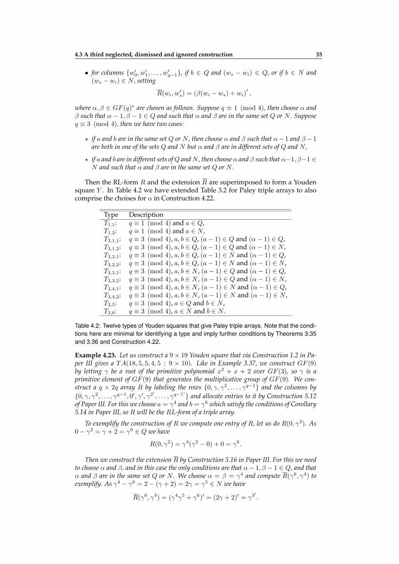
4.3 A third neglected, dismissed and ignored construction 35

• for columns w′0, w

′1, . . . , w

′q−1, if b ∈ Q and (ws − wi) ∈ Q, or if b ∈ N and

(ws − wi) ∈ N , setting

R(wi, w′s) = (β(wi − ws) + wi)

′,

where α, β ∈ GF (q)∗ are chosen as follows. Suppose q ≡ 1 (mod 4), then choose α andβ such that α− 1, β − 1 ∈ Q and such that α and β are in the same set Q or N . Supposeq ≡ 3 (mod 4), then we have two cases:

⋆ if a and b are in the same set Q or N , then choose α and β such that α− 1 and β− 1are both in one of the sets Q and N but α and β are in different sets of Q and N ,

⋆ if a and b are in different sets of Q and N , then choose α and β such that α−1, β−1 ∈N and such that α and β are in the same set Q or N .

Then the RL-form R and the extension R are superimposed to form a Youdensquare Y . In Table 4.2 we have extended Table 3.2 for Paley triple arrays to alsocomprise the choises for α in Construction 4.22.

Type DescriptionT1,1: q ≡ 1 (mod 4) and a ∈ Q,T1,2: q ≡ 1 (mod 4) and a ∈ N ,T3,1,1: q ≡ 3 (mod 4), a, b ∈ Q, (a− 1) ∈ Q and (α− 1) ∈ Q,T3,1,2: q ≡ 3 (mod 4), a, b ∈ Q, (a− 1) ∈ Q and (α− 1) ∈ N ,T3,2,1: q ≡ 3 (mod 4), a, b ∈ Q, (a− 1) ∈ N and (α− 1) ∈ Q,T3,2,2: q ≡ 3 (mod 4), a, b ∈ Q, (a− 1) ∈ N and (α− 1) ∈ N ,T3,3,1: q ≡ 3 (mod 4), a, b ∈ N , (a− 1) ∈ Q and (α− 1) ∈ Q,T3,3,2: q ≡ 3 (mod 4), a, b ∈ N , (a− 1) ∈ Q and (α− 1) ∈ N ,T3,4,1: q ≡ 3 (mod 4), a, b ∈ N , (a− 1) ∈ N and (α− 1) ∈ Q,T3,4,2: q ≡ 3 (mod 4), a, b ∈ N , (a− 1) ∈ N and (α− 1) ∈ N ,T3,5: q ≡ 3 (mod 4), a ∈ Q and b ∈ N ,T3,6: q ≡ 3 (mod 4), a ∈ N and b ∈ N .

Table 4.2: Twelve types of Youden squares that give Paley triple arrays. Note that the condi-tions here are minimal for identifying a type and imply further conditions by Theorems 3.35and 3.36 and Construction 4.22.

Example 4.23. Let us construct a 9× 19 Youden square that via Construction 1.2 in Pa-per III gives a TA(18, 5, 5, 4, 5 : 9 × 10). Like in Example 3.37, we construct GF (9)by letting γ be a root of the primitive polynomial x2 + x + 2 over GF (3), so γ is aprimitive element of GF (9) that generates the multiplicative group of GF (9). We con-struct a q × 2q array R by labeling the rows 0, γ, γ2, . . . , γq−1 and the columns by0, γ, γ2, . . . , γq−1, 0′, γ′, γ2′ , . . . , γq−1′ and allocate entries to it by Construction 5.12of Paper III. For this we choose a = γ4 and b = γ6 which satisfy the conditions of Corollary5.14 in Paper III, so R will be the RL-form of a triple array.

To exemplify the construction of R we compute one entry of R, let us do R(0, γ2). As0− γ2 = γ + 2 = γ6 ∈ Q we have

R(0, γ2) = γ4(γ2 − 0) + 0 = γ6.

Then we construct the extension R by Construction 5.16 in Paper III. For this we needto choose α and β, and in this case the only conditions are that α− 1, β − 1 ∈ Q, and thatα and β are in the same set Q or N . We choose α = β = γ4 and compute R(γ6, γ4) toexemplify. As γ4 − γ6 = 2− (γ + 2) = 2γ = γ5 ∈ N we have

R(γ6, γ4) = (γ4γ5 + γ6)′ = (2γ + 2)′ = γ3′ .

36 Research questions and summary of papers I-III

Finally, we superimpose R and R, which includes that we add a first column ∞ =

(0′, γ′, . . . , γ8′) to get the q×2q + 1 Youden square Y here below. Applying Construction1.2 in Paper III to Y modulo column ∞ gives the RL-form of the Paley triple array of typeT1,1 in Example 3.37.

0′ ∞ γ5′ γ6 γ7′ γ8 γ′ γ2 γ3′ γ4 0 γ3 γ6′ γ5 γ8′ γ7 γ2′ γ γ4′

γ′ γ5′ ∞ γ4′ γ8 γ2′ 0′ γ7 γ6 γ3 γ2 γ γ5 γ8′ 0 γ4 γ7′ γ6′ γ3′

γ2′ γ6 γ4′ ∞ γ5 γ′ γ3 0 γ8′ γ7′ γ6′ γ7 γ2 γ5′ γ8 γ3′ 0′ γ4 γ

γ3′ γ7′ γ8 γ5 ∞ γ6′ γ2 γ4′ 0′ γ γ4 γ8′ γ5′ γ3 γ7 γ2′ 0 γ6 γ8′

γ4′ γ8 γ2′ γ′ γ6′ ∞ γ7 γ3′ γ5 0 γ8′ γ6 γ3 γ γ4 γ7′ γ2 γ5′ 0′

γ5′ γ′ 0′ γ3 γ2 γ7 ∞ γ8′ γ4 γ6′ γ6 γ8 γ3′ γ2′ γ7′ γ5 γ γ4′ 0

γ6′ γ2 γ7 0 γ4′ γ3′ γ8′ ∞ γ γ5′ γ2′ γ7′ 0′ γ8 γ5 γ3 γ6 γ′ γ4

γ7′ γ3′ γ6 γ8′ 0′ γ5 γ4 γ ∞ γ2′ γ8 γ6′ 0 γ2 γ5′ γ4′ γ′ γ7 γ3

γ8′ γ4 γ3 γ7′ γ 0 γ6′ γ5′ γ2′ ∞ γ4′ γ3′ γ6 γ′ 0′ γ2 γ7 γ5 γ8

Author’s contributions to this paper: This paper was a collaborative effort, andall ideas and results were discussed with my co-author. The construction of Paleytriple arrays as well as the result on projective planes and difference sets wereinitiated and carried out by me.

Part II

Solitons

37

Chapter 5

Introduction to an operatortheoretic approach to solitontheory

“True laws of Nature cannot be linear.”Albert Einstein

5.1 Historical background

In 1834, when John Scott Russel was trying to find the most suitable design forcanal boats, he made experiments at the Union Canal near Edinburgh. One daywhen he was sitting on his horse close to the canal, he happened to catch sight ofa peculiar wave phenomenon.

“I was observing the motion of a boat which was rapidly drawn along a narrowchannel by a pair of horses, when the boat suddenly stopped – not so the massof water in the channel which it had put in motion; it accumulated round theprow of the vessel in a state of violent agitation, then suddenly leaving it be-hind, rolled forward with great velocity, assuming the form of a large solitaryelevation, a rounded, smooth and well-defined heap of water, which continuedits course along the channel apparently without change of form or diminuationof speed. I followed it on hourseback, and overtook it still rolling on at a rate ofsome eight or nine miles an hour, preserving its original figure some thirty feetlong and a foot to a foot and a half in height. Its heights gradually diminished,and after a chase of one or two miles I lost it in the windlings of the channel.”- J. S. Russel, “Reports on Waves”, (14th Meeting of the British Associ-ation for the Advancement of Science, 1844)

Certainly, Russel was not the first to observe such a wave in nature, but he seemsto be the first to draw the interest of a larger scientific audience to the phenomenonof these solitary waves or wave of translation as he also called them. As a solid sci-entist and engineer, he built a long wave tank in his back garden where he wasable to reproduce such waves in experiments. He guessed a mathematical descrip-tion of their shape, which was confirmed by much later achievements in the topic.Actually it takes quite a while, until Korteweg and de Vries [69] derive the dif-

38

5.2 The operator method 39

ferential equation governing the dynamics of shallow water waves. Despite this

Figure 5.1: Simulation of J. S. Russel’s observation (Heriot–Watt University 1995).

important conceptual progress, the start of modern soliton theory is usually lo-cated at the celebrated Fermi-Pasta-Ulam experiments [61]. Their surprising out-come strikingly underlines that stability phenomena, such as the existence of local-ized shape-preserving waves, should be of principle importance in mathematicalphysics. Shortly afterwards, the famous inverse scattering method is developed byGardner, Green, Kruskal and Miura [63]. From that moment on, the topic of inte-grable systems has been a very active research area with quick progress and manybrilliant discoveries linking the topic to several major parts of mathematics likedifferential geometry, algebraic geometry and topology, representation theory andoperator theory. In parallel, physicists continue to discover applications in disci-plines as varied as quantum optics, general relativity, crystallography, biophysics(see for example [62] and references therein).

5.2 The operator method

The present work is based on an operator method for the study of soliton equationswhich can be described as follows:

1. The starting point is a the soliton equation one is interested in together witha solution u of this equation. Typically this solution is the 1-soliton solution,which depends on a parameter a ∈ C.

2. The first step consists in finding a noncommutative counterpart of the givensoliton equation. More precisely, one looks for a differential equation forfunctions with values in some suitable (not necessarily commutative) algebraA which reduces to the original equation if A = C.

Simultaneously one looks for a noncommutative counterpart U of u such thatU solves the noncommutative equation. Typically, in this process the scalarparameter a is blown up to a parameter A ∈ A.

3. The second step is to construct a solution formula for the original equationby applying a suitable functional τ : A 7→ C to U . The crucial point is to do itin such a way that the solution property is maintained.

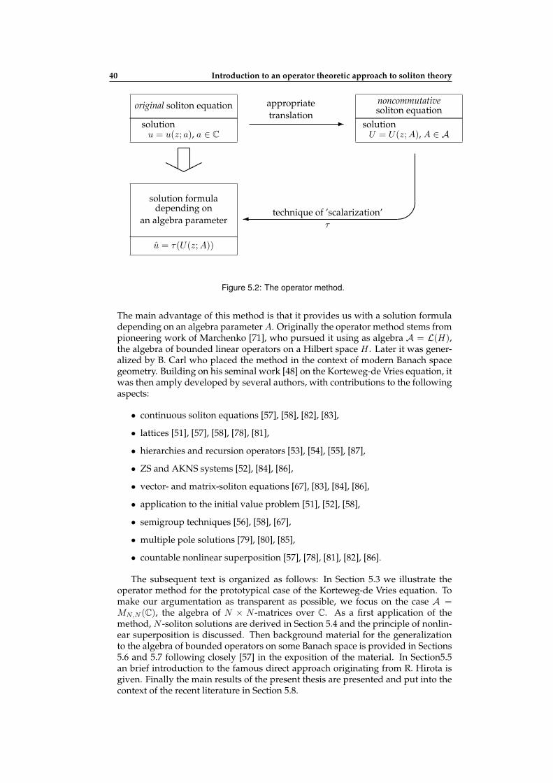
40 Introduction to an operator theoretic approach to soliton theory

original soliton equation

solutionu = u(z; a), a ∈ C

solution formuladepending on

an algebra parameter

u = τ(U(z;A))

noncommutativesoliton equation

solutionU = U(z;A), A ∈ A

appropriatetranslation

technique of ’scalarization’τ

-

!

HH

Figure 5.2: The operator method.

The main advantage of this method is that it provides us with a solution formuladepending on an algebra parameter A. Originally the operator method stems frompioneering work of Marchenko [71], who pursued it using as algebra A = L(H),the algebra of bounded linear operators on a Hilbert space H . Later it was gener-alized by B. Carl who placed the method in the context of modern Banach spacegeometry. Building on his seminal work [48] on the Korteweg-de Vries equation, itwas then amply developed by several authors, with contributions to the followingaspects:

• continuous soliton equations [57], [58], [82], [83],

• lattices [51], [57], [58], [78], [81],

• hierarchies and recursion operators [53], [54], [55], [87],

• ZS and AKNS systems [52], [84], [86],

• vector- and matrix-soliton equations [67], [83], [84], [86],

• application to the initial value problem [51], [52], [58],

• semigroup techniques [56], [58], [67],

• multiple pole solutions [79], [80], [85],

• countable nonlinear superposition [57], [78], [81], [82], [86].

The subsequent text is organized as follows: In Section 5.3 we illustrate theoperator method for the prototypical case of the Korteweg-de Vries equation. Tomake our argumentation as transparent as possible, we focus on the case A =MN,N (C), the algebra of N × N -matrices over C. As a first application of themethod, N -soliton solutions are derived in Section 5.4 and the principle of nonlin-ear superposition is discussed. Then background material for the generalizationto the algebra of bounded operators on some Banach space is provided in Sections5.6 and 5.7 following closely [57] in the exposition of the material. In Section5.5an brief introduction to the famous direct approach originating from R. Hirota isgiven. Finally the main results of the present thesis are presented and put into thecontext of the recent literature in Section 5.8.

5.3 Illustration of the method for the Korteweg-de Vries equation 41

Figure 5.3: Snapshot of the 1-soliton solution of the Korteweg-de Vries equation.

5.3 Illustration of the method for the Korteweg-deVries equation

In this section we implement the operator method in the prototypical case of theKorteweg-de Vries equation,

ut = uxxx + 6uux. (5.1)

The results are due to Aden and Carl [48] who implemented the method for thefirst time for the potential Korteweg-de Vries equation, see also [57] for a presen-tation for the Korteweg-de Vries equation itself.

The 1-soliton solution of the Korteweg-de Vries equation reads

u(x, t) =a2

2cosh−2

(a2(x+ a2t+ φ)

). (5.2)

Note that the solution depends on two real parameters a, φ, the first characterizingits height and velocity, the second its initial position.

5.3.1 The noncommutative Korteweg-de Vries equation and thenoncommutative analogue of its soliton solution

The noncommutative Korteweg-de Vries equation reads

Ut = Uxxx + 3(UUx + UxU), (5.3)

where U is a function with values in the N ×N -matrices over C. Note that this isa very canonical noncommutative interpretation of (5.1) where noncommutativityis reflected by replacing the nonlinear term in a symmetric way.

The following reformulation of (5.2) motivates the noncommutative interpre-tation of the soliton solution. Setting ℓ(x, t) = exp(ax + a3t)b, where b = exp(aφ),one finds

u(x, t) = 2a2

(√ℓ(x, t) +

1√ℓ(x, t)

)−2

= 2a2 (1 + ℓ(x, t))−2

ℓ(x, t)

=∂

∂x

((1 + ℓ(x, t)

)−12aℓ(x, t)

).

Hence, a reasonable noncommutative counterpart is

U(x, t) =∂

∂x

((I + L(x, t)

)−1 (AL(x, t) + L(x, t)A

)), (5.4)

42 Introduction to an operator theoretic approach to soliton theory

where L(x, t) = exp(Ax+A3t)B and A,B are constant N ×N -matrices. Of course,in the matrix case invertibility of I + L(x, t) is no longer a priori guaranteed.

The next proposition, which is a corollary of [48, Theorem III B 2 (i)], see also[57, Proposition 5.1], states the solution property of (5.4).

Proposition 5.1. Let A,B be N × N -matrices and define L(x, t) = exp(Ax + A3t)B.Then (5.4) is a solution of the noncommutative Korteweg-de Vries equation (5.3) on Ω =(x, t) ∈ R2 | det

(I + L(x, t)

)= 0.

Proof. Let V = (I + L)−1(AL + LA). Using Lx = AL and the noncommutativederivation rule for inverses

((IL)

−1)= −(I + L)−1Lx(I + L)−1 we obtain

Vx = −(I + L)−1Lx(I + L)−1(AL+ LA) + (I + L)−1(ALx + LxA)

= −(I + L)−1AL(I + L)−1(AL+ LA) + (I + L)−1A(AL+ LA)

= (I + L)−1A(I + L)−1(AL+ LA)

= (I + L)−1AV,

where we have used the identity L(I + L)−1 = I − (I + L)−1 to replace the termL(I + L)−1 in the above calculation. Similarly,

Vxx = 2(I + L)−1A(I + L)−1AV − V A2V,

Vxxx = 6(I + L)−1A(I + L)−1A(I + L)−1AV

−3(I + L)−1A2(I + L)−1AV − 3(I + L)−1A(I + L)−1A2V

+(I + L)−1A3V

andVt = (I + L)−1A3(I + L)−1(AL+ LA).

On the other hand,

V 2x = (I + L)−1A(I + L)−1(AL+ LA)(I + L)−1AV

= (I + L)−1A(I + L)−1(A(I + L) + (I + L)A− 2A

)(I + L)−1AV

= (I + L)−1A(I + L)−1A2V + (I + L)−1A2(I + L)−1AV

−(I + L)−1A(I + L)−1A(I + L)−1AV.

In summary this shows that V is a solution of the noncommutative potential Korteweg-de Vries equation

Vt = Vxxx + 3V 2x .

From this we infer that Vtx = Vxxxx+3(VxxVx+VxVxx) using the noncommutativeproduct rule. In other words U = Vx solves (5.3).

5.3.2 Derivation of a solution formula for the scalar Korteweg-de Vries equation

To derive a solution formula for the Korteweg-de Vries equation (5.1), the mainidea is to apply a (linear) functional τ : MN,N (C) 7→ C to a solution of the non-commutative Korteweg-de Vries equation (5.3). Of course the key point is to dothis in such a way that the solution property is maintained.

As a motivation we start from the observation that, if U(x, t) is a solution ofthe noncommutative Korteweg-de Vries equation (5.3), then so is T−1U(x, t)T forevery constant invertible matrix T . In other words, conjugation with a constant

5.3 Illustration of the method for the Korteweg-de Vries equation 43

matrix does not change the solution property. Thus it is reasonable to look for afunctional τ that maps U(x, t) and T−1U(x, t)T to the same scalar function u(x, t).The next lemma shows that this restricts the choice of the functional considerably.

Lemma 5.2. Let τ : MN,N (C) 7→ C be a linear functional with τ(ST ) = τ(TS) for allN ×N -matrices S, T . Then τ is a multiple of the trace tr.

Proof. Let the function τ be given by τ(T ) =∑N

i,j=1 λijtij for T = (tij)Ni,j=1. De-

note by Eij the matrix with the only non-vanishing entry 1 in the ith row and jthcolumn. Then λij = τ(Eij) = τ(EiiEij) = τ(EijEii) = τ(δijEii) = δij = 0 forj = i and λjj = τ(Ejj) = τ(Ej1E1j) = τ(E1jEj1) = τ(E11) = λ11 for all j, Henceτ(T ) = λ11

∑Nj=1 tjj = λ11tr(T ).

In the case N = 1, the fact that τ maintains the solution property necessar-ily means that τ is the identity map. In view of the above motivation, the rightgeneralization for N > 1 appears to be the trace tr.

The difficulty is that in order to maintain the solution property, τ needs to bemultiplicative at least to a certain extent. However, since the trace is not multi-plicative on all of MN,N (C), we need to restrict the class of matrices.

To this end we need some notation. A matrix T is called one-dimensional, if itsrange ran(T ) = Tv | v ∈ CN is a one-dimensional subspace of CN . Note that forran(T ) = spanc we have T = cat where the entries of the vector a are given byTej = ajc. Since ker(T ) = v ∈ CN | ⟨a, v⟩ = 0, the kernel of T is determinedby a. Vice versa, two one-dimensional matrices S, T with the same kernel can bewritten in the form S = cat, T = dat with the same vector a. Finally we observethat for T = cat the trace can be calculated by the simple formula tr(T ) = atc.

Lemma 5.3. On the set of one-dimensional matrices with the same kernel, the trace ismultiplicative.

Proof. Let S = cat, T = dat. Then ST = (cat)(dat) = c(atd)at = tr(T )cat = tr(T )S.Hence, tr(ST ) = tr

(tr(T )S

)= tr(S)tr(T ).

The following proposition ([48, Proposition III B 1], see also [57, Proposition5.2]) is a summary of the above discussion.

Proposition 5.4. If U = U(x, t) is a solution of the noncommutative Korteweg-de Vriesequation (5.3) which is one-dimensional with constant kernel, then u = tr(U) is a solutionof the scalar Korteweg-de Vries equation (5.1).

Proof. By assumption U can be written in the form U(x, t) = c(x, t)at with someconstant vector a and a vector function c = c(x, t). But then Ux(x, t) = cx(x, t)a

t,which means that U , Ux are one-dimensional with the same kernel. By Lemma 5.3,tr(UUx) = tr(UxU) = tr(U)tr(Ux). As a linear functional on MN,N (C), the trace iscontinuous. Thus tr(Ux) = tr(U)x. Together, this shows

ut = tr(U)t = tr(Ut)(5.3)= tr

(Uxxx + 3(UUx + UxU)

)= tr(Uxxx) + 3

(tr(UUx) + tr(UxU)

)= tr(U)xxx + 6 tr(U)tr(U)x

= uxxx + 6uux.

44 Introduction to an operator theoretic approach to soliton theory

Applying Proposition 5.4 to the concrete solution (5.4) yields the desired solu-tion formula. This is the contents of the next theorem. See [48, Theorem III B 2 (ii)],[57, Theorem 5.4] for a corresponding solution formula in the more general contextof quasi-Banach ideals.

Theorem 1. Let A,B be N × N -matrices such that AB + BA is one-dimensional, anddefine L(x, t) = exp(Ax+A3t)B. Then

u(x, t) = 2∂2

∂x2log det

(I + L(x, t)

)is a solution of the Korteweg-de Vries equation (5.1) on Ω = (x, t) ∈ R2 | det

(I +

L(x, t))= 0.

Proof. For AB+BA = cat, it is straightforward to verify that the solution (5.4) hasthe form U(x, t) = dx(x, t)a

t with the vector-function

d(x, t) =(I + exp(Ax+A3t)B

)−1exp(Ax+A3t)c.

Thus the assumptions of Proposition 5.4 are satisfied and we get a solution u of theKorteweg-de Vries equation (5.1) by taking the trace of U . On the other hand, fromthe representation (5.4), we find

u = tr(U)

=∂

∂xtr((I + L)−1(AL+ LA)

)=

∂

∂x

(tr((I + L)−1AL

)+ tr

((I + L)−1LA

)).

Since L and (I + L)−1 commute, we observe tr((I + L)−1LA

)= tr

(L(I + L)−1A

),

and, using the trace property, then tr(L · (I +L)−1A

)= tr

((I +L)−1A ·L

). Hence,

u = 2∂

∂xtr((I + L)−1AL

)= 2

∂

∂xtr((I + L)−1Lx

).

To complete the proof, it remains to apply the subsequent lemma.

Lemma 5.5. Let T = T (x) be a matrix-function which is differentiable and invertible insome open interval J in R. Then, for all x ∈ J , it holds(

det(T (x)

))−1 d

dxdet(T (x)

)= tr

(T−1(x)

d

dxT (x)

).

Proof. Fix x0 ∈ J and set S(x) = T−1(x0)T (x). Note that then S(x0) = IN . WritingS(x) = (S(1)(x), . . . , S(N)(x)) where S(j)(x) is the jth column of S(x), we thushave S(j)(x0) = ej , the jth standard unit vector, and

(det(T (x0))

)−1 d

dx

∣∣∣x=x0

det(T (x)

)=

=d

dx

∣∣∣x=x0

det(S(x)

)=

d

dx

∣∣∣x=x0

det(S(1)(x), . . . , S(N)(x)

)

5.4 N -soliton solutions and nonlinear superposition 45

=N∑j=1

det(S(1)(x0), . . . , S

(j−1)(x0),d

dx

∣∣∣x=x0

S(j)(x), S(j+1)(x0), . . . , S(N)(x0)

)

=N∑j=1

det(e1, . . . , ej−1,

d

dx

∣∣∣x=x0

S(j)(x), ej+1, . . . , eN

)= tr

( d

dx

∣∣∣x=x0

S(x))

= tr(T−1(x0)

d

dxT (x0)

).

5.4 N -soliton solutions and nonlinear superposition

In this section we rederive the well-known N -soliton solutions of Hirota [65] byinserting diagonal matrices A into the solution formula in Proposition 1 and studytheir collision behavior for N = 2 and N = 3.

Let

A =

k1 0. . .

0 kN

.

where kj ∈ C are pairwise different and ki + kj = 0 for all i, j = 1, . . . , N .

In order to satisfy the one-dimensionality condition of Theorem 1, we considerthe Sylvester equation

AX +XA = C (5.5)

for a given right-hand side C. Of course we are mainly interested in the case thatC is one-dimensional. However, it is well-known that (5.13) is uniquely solvable ifand only if 0 ∈ spec(A) + spec(A) (see for example [50] for a survey on Sylvester’sequation in the matrix case).

In our situation, spec(A) + spec(A) = ki + kj | i, j = 1, . . . , N showing that(5.13) is always solvable. Indeed, it is straightforward to verify that, for a, c ∈ CN

arbitrary, the unique solution B of

AB +BA = cat

is given by

B =

(ajci

ki + kj

)N

i,j=1

.

Thus, according to Theorem 1, a solution of the Korteweg-de Vries equation isgiven by u(x, t) = 2∂2

x log p(x, t), where

p(x, t) = det

((δij + exp

(kix+ k3i t

) ajciki + kj

)N

i,j=1

)

= 1 +N∑

m=1

∑i1<...<im

det

(exp(kijx+ k3ij t) aij′ cij

kij + kij′

)m

j,j′=1

= 1 +

N∑m=1

∑i1<...<im

m∏j=1

aijcij exp(kijx+ k3ij t

)det

( 1

kij + kij′

)m

j,j′=1

46 Introduction to an operator theoretic approach to soliton theory

= 1 +N∑

m=1

∑i1<...<im

m∏j=1

aijcij2kij

exp(kijx+ k3ij t

) m∏j′=j+1

(kij − kij′

kij + kij′

)2

where we refer to [75] for the identity

det

((1

ki + kj

)m

i,j=1

)=

m∏i=1

1

2ki

m∏j=i+1

(ki − kjki + kj

)2

which has been used in the last step.

Abbreviating Aij =((ki − kj)/(ki + kj)

)2 and ℓj(x, t) = exp(kjx + k3j t + δj),where δj is defined by exp(δj) = (ajcj)/(2kj), we find

p(x, t) = 1 +N∑

m=1

∑i1<...<im

m∏j=1

ℓij (x, t)m∏

j′=j+1

Aijij′ .

For 0 < k1 < . . . < kN and δj ∈ R this solution is the famous N -soliton solution ofHirota.

Let us take a closer look at the 2-soliton solution. As shown in Figure 5.4, forlarge negative times the solution consists of two single solitons which are well sep-arated and travel each with constant velocity. As time goes by, the faster solitoncatches up with the smaller one and overtakes it. The resulting collision does nei-ther change the shape nor the velocity of the solitons, its only effect is that theboth solitons experience a phase shift: The faster one is shifted forward, the slowerone backward. For large positive times the picture is the same as in the beginningexcept that the solitons appear in reversed order.

In the generic situation where one soliton is much larger than the other, a singlemaximum is formed during collision. However, if the difference of height betweenthe solitons is small there are always two maxima present, see Figure 5.5. For moredetails we refer to [49] and references therein.

We conclude the section with an illustration of the 3-soliton solution in Fig-ure 5.6.

5.5 Hirota’s bilinear method

In this section we explain the connection between the operator method and thecelebrated bilinear method of Hirota, a direct method for constructing N -solitonsolutions. Introduced by Hirota [65] for the Korteweg-de Vries equation, it hassince become one of the most powerful direct methods in soliton theory. For asurvey on the state of art we refer to [66], see also [72].

To start with, we introduce the D-operator (or Hirota derivative), a binary differ-ential operator acting on a pair of functions a(x, t), b(x, t) which is defined by

Dmx Dn

t (a, b) =

(∂

∂x− ∂

∂x′

)m(∂

∂t− ∂

∂t′

)n

a(x, t)b(x′, t′)

∣∣∣∣∣∣ x=x′

t=t′

.

As an illustration, we calculate DxDt(a, b). Since(∂

∂x− ∂

∂x′

)(∂

∂t− ∂

∂t′

)a(x, t)b(x′, t′)

5.5 Hirota’s bilinear method 47

Figure 5.4: Two typical interaction patterns for the 2-soliton solution. On the left we havechosen k1 = 0.5, k2 = 1, on the right k1 = 0.5, k2 = 0.7. In both cases the solution is shownat succeeding times.

48 Introduction to an operator theoretic approach to soliton theory

Figure 5.5: The same 2-soliton solutions as in Figure 5.4 depicted over the xt-plane.

Figure 5.6: 3-soliton solution for k1 = 0.5, k2 = 0.7 and k3 = 1 shown over the xt-plane.

=

(∂

∂x− ∂

∂x′

)(at(x, t)b(x

′, t′)− a(x, t)bt′(x′, t′)

)= atx(x, t)b(x

′, t′)− ax(x, t)bt′(x′, t′)− at(x, t)bx′(x′, t′) + a(x, t)bt′x′(x′, t′),

we getDxDt(a, b) =

(axtb+ abxt

)−(axbt + atbx

)(5.6)

For a more thorough discussion of the D-operators properties see [66], [72].

Hirota showed that in many cases a soliton equation can be rewritten, via anappropriate transformation of variables, in terms of the D-operator. This processis called bilinearization.

For the Korteweg-de Vries equation, substitution of the logarithmic transfor-mation

u = 2∂2

∂x2log f (5.7)

5.5 Hirota’s bilinear method 49

into (5.1), one obtains after one integration in x (the integration constant denotedby c) and a little manipulation

ffxt − fxft = ffxxxx − 4fxfxxx + 3f2xx + cf2.

In view of (5.6), the left-hand side of the above equation coincides with DxDt(f, f)up to a factor 1/2. Similarly, it is straightforward to express also its the right-handside in terms of the D-operator. As a result,

DxDt(f, f) = D4x(f, f) + cf2,

and taking into account the boundary conditions for obtaining soliton solutions,fx, fxx, . . . → 0 for x → ±∞, we arrive at the bilinear form of the Korteweg-deVries equation

Dx

(Dt −D3

x

)(f, f) = 0. (5.8)

Vice versa, if f solves (5.8), a solution u of the Korteweg-de Vries equation is ob-tained by (5.7).

To solve (5.8), one uses a formal perturbation expansion ansatz. Inserting theexpression

f(x, t) =

∞∑n=0

ϵnfn(x, t) (5.9)

with f0(x, t) ≡ 1, and comparing coefficients in the powers of ϵ, (5.8) is turned intoa hierarchy of equations for fn(x, t) (n ≥ 1), which can be solved successively.

In particular, starting from

f1(x, t) =N∑j=1

exp(ηj),

the series (5.9) terminates and yields the N -soliton solutions [65], see also [66, Sec-tion 1.8] for details, as given in the next proposition.

Proposition 5.6. Let 0 < k1 < . . . < kN and φ1, . . . , φN ∈ R. The N -soliton solutionof the bilinear form (5.8) of the Korteweg-de Vries equation is given by

f(x, t) =∑µ=0,1

exp( N∑

j=1

µjηj +

(N)∑i<j

µiµjAij

),

where

ηj = kjx+ k3j t+ φj

exp(Aij) =

(ki − kjki + kj

)2

,

and where the sum is taken over all possible vectors µ = (µ1, . . . , µN ) ∈ 0, 1N .

The following proposition shows that the operator method also yields solutionsof Hirota’s bilinear form.

Proposition 5.7. Let A,B be N ×N -matrices such that AB + BA is one-dimensional,and define L(x, t) = exp(Ax+A3t)B. Then

f(x, t) = det(I + L(x, t)

)is a solution of the bilinear Korteweg-de Vries equation (5.8).

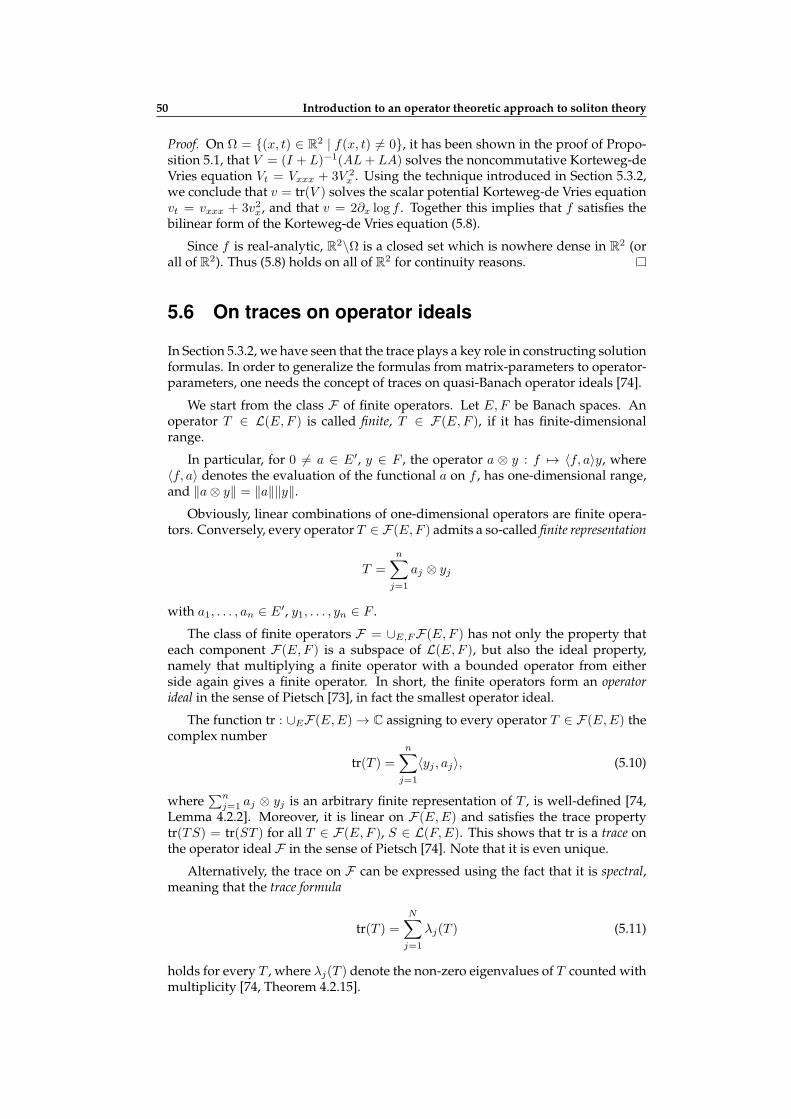
50 Introduction to an operator theoretic approach to soliton theory

Proof. On Ω = (x, t) ∈ R2 | f(x, t) = 0, it has been shown in the proof of Propo-sition 5.1, that V = (I + L)−1(AL+ LA) solves the noncommutative Korteweg-deVries equation Vt = Vxxx + 3V 2

x . Using the technique introduced in Section 5.3.2,we conclude that v = tr(V ) solves the scalar potential Korteweg-de Vries equationvt = vxxx + 3v2x, and that v = 2∂x log f . Together this implies that f satisfies thebilinear form of the Korteweg-de Vries equation (5.8).

Since f is real-analytic, R2\Ω is a closed set which is nowhere dense in R2 (orall of R2). Thus (5.8) holds on all of R2 for continuity reasons.

5.6 On traces on operator ideals

In Section 5.3.2, we have seen that the trace plays a key role in constructing solutionformulas. In order to generalize the formulas from matrix-parameters to operator-parameters, one needs the concept of traces on quasi-Banach operator ideals [74].

We start from the class F of finite operators. Let E,F be Banach spaces. Anoperator T ∈ L(E,F ) is called finite, T ∈ F(E,F ), if it has finite-dimensionalrange.

In particular, for 0 = a ∈ E′, y ∈ F , the operator a ⊗ y : f 7→ ⟨f, a⟩y, where⟨f, a⟩ denotes the evaluation of the functional a on f , has one-dimensional range,and ∥a⊗ y∥ = ∥a∥∥y∥.

Obviously, linear combinations of one-dimensional operators are finite opera-tors. Conversely, every operator T ∈ F(E,F ) admits a so-called finite representation

T =

n∑j=1

aj ⊗ yj

with a1, . . . , an ∈ E′, y1, . . . , yn ∈ F .

The class of finite operators F = ∪E,FF(E,F ) has not only the property thateach component F(E,F ) is a subspace of L(E,F ), but also the ideal property,namely that multiplying a finite operator with a bounded operator from eitherside again gives a finite operator. In short, the finite operators form an operatorideal in the sense of Pietsch [73], in fact the smallest operator ideal.

The function tr : ∪EF(E,E) → C assigning to every operator T ∈ F(E,E) thecomplex number

tr(T ) =n∑

j=1

⟨yj , aj⟩, (5.10)

where∑n

j=1 aj ⊗ yj is an arbitrary finite representation of T , is well-defined [74,Lemma 4.2.2]. Moreover, it is linear on F(E,E) and satisfies the trace propertytr(TS) = tr(ST ) for all T ∈ F(E,F ), S ∈ L(F,E). This shows that tr is a trace onthe operator ideal F in the sense of Pietsch [74]. Note that it is even unique.

Alternatively, the trace on F can be expressed using the fact that it is spectral,meaning that the trace formula

tr(T ) =N∑j=1

λj(T ) (5.11)

holds for every T , where λj(T ) denote the non-zero eigenvalues of T counted withmultiplicity [74, Theorem 4.2.15].

5.6 On traces on operator ideals 51

Both of the two possibilities (5.10), (5.11) to represent the trace on F indicate anatural approach to extend the trace to larger quasi-Banach operator ideals. In thesequel we hint at some obstacles and results in this direction. Actually the generalextension problem is very subtle. For a more detailed report, we refer to [58].

5.6.1 Spectral traces

In order to define the spectral trace on a quasi-Banach operator ideal A, we need toassociate to every operator T ∈ A(E,E) its eigenvalue sequence (λj(T ))j . A rathergeneral class of operators for which this can be done are the so-called Riesz opera-tors, see [74, Chapter 3.2] for details. Moreover, we obviously need the eigenvaluesequence to be absolutely summing.

We say that the quasi-Banach operator ideal A has eigenvalue type ℓ1 if everyoperator T ∈ A(E,E) is a Riesz operator with eigenvalue sequence in ℓ1. In thissituation, a deep result of White [88] states that the trace formula indeed defines acontinuous trace on A.

However, a counterexample of Kalton [68] shows that in general this trace isnot unique.

5.6.2 Traces for nuclear operators

The formula (5.10) motivates to consider the class Nr = ∪E,FNr(E,F ) of r-nuclearoperators (0 < r ≤ 1). We say that an operator T ∈ L(E,F ) belongs to Nr(E,F ) ifit admits a representation

T =∞∑j=1

aj ⊗ yj with∞∑j=1

∥aj∥r∥yj∥r < ∞

and a1, a2, . . . ∈ E′, y1, y2, . . . ∈ F . Nr becomes an r-Banach operator ideal withrespect to the r-norm

∥ T | Nr ∥ = inf( ∞∑

j=1

∥aj∥r∥yj∥r) 1

r

,

where the infimum is taken over all possible representations of T . In fact, Nr is thesmallest r-Banach operator ideal.

However, as an example by Enflo [59] shows, on N = N1 the assignment

trN (T ) =∞∑j=1

⟨yj , aj⟩ (5.12)

is only independent of the chosen representation T =∑∞

j=1 aj ⊗ yj , if one restrictsto Banach spaces with approximation property1. If this is the case, trN defines aunique continuous trace [74, Theorem 4.7.2]. Note that this trace is not spectral asan example by Enflo [59] shows.

On the other hand, the assignment (5.12) is well-defined on the smaller r-Banach operator ideals Nr (over the class of all Banach spaces) if 0 < r ≤ 2

3 ,where it yields a unique trace. In view of the fact that Nr has eigenvalue typeℓ1 for 0 < r ≤ 2

3 , this trace is even spectral.

1A Banach space E has the approximation property if, for all precompact K ⊂ E and all ϵ > 0 there isa finite operator T such that ∥x− Tx∥ ≤ ϵ for all x ∈ K

52 Introduction to an operator theoretic approach to soliton theory

5.6.3 Determinants and their relationship to traces

Similarly as with traces, there is an axiomatic approach to determinants on quasi-Banach operator ideals [74]. The Trace-determinant theorem clarifies their relation-ship. It states that there is a one-to-one correspondence between continuous tracesand continuous determinants on every quasi-Banach operator ideal.

To conclude this section we state the generalization of Lemma 5.5. Let A be aquasi-Banach operator ideal admitting a continuous determinant δ, and let T =T (x) be an A(E)-valued function which is differentiable and invertible in someopen interval J in R. Then, for all x ∈ J , it holds(

δ(I + T (x)

))−1 d

dxδ(I + T (x)

)= τ

((I + T (x)

)−1 d

dxT (x)

)where τ demotes the continuous trace on A given by the Gâteaux derivative

τ(S) = limξ→0

δ(I + ξS)− 1

ξ

for S ∈ A(E,E).

5.7 On elementary operators and Sylvester’s equa-tion

To apply the solution formula in Theorem 1, we need that AB+BA is one-dimensional.This leads us to consider Sylvester’s equation

AX +XB = Y. (5.13)

Here A ∈ L(E), B ∈ L(F ) are given bounded linear operators on some Banachspaces E, F . In this context Rosenblum’s theorem [76] provides a sufficient con-dition: (5.13) has a unique solution X for each given right-hand side Y providedthat 0 ∈ spec(A) + spec(B).

For a generalization of Theorem 1 to operator-parameters, it is decisive to knowwhether the solution of (5.13) belongs to a quasi-Banach ideal admitting a contin-uous determinant. To this end, we slightly change viewpoint.

Let A be a p-Banach operator ideal, 0 < p ≤ 1, and consider the elementaryoperator ΦA,B : A(F,E) −→ A(F,E) defined by

ΦA,B(X) = AX +XB.

A result of Aden [47], see also Eschmeier [60] for the case p = 1, states that, inde-pendently of the underlying p-Banach operator ideal A,

spec(ΦA,B) = spec(A) + spec(B).

The crucial consequence for the task at hand is, that, under the assumption 0 ∈spec(A) + spec(B), the operator equation AX +XB = C is not only always solv-able, but for the solution Φ−1

A,B(C) it holds that

Φ−1A,B(C) ∈ A(F,E)

for any p-Banach operator ideal A.

For hints on alternative approaches to solve Sylvester’s equation on quasi-Banach ideals without the condition 0 ∈ spec(A) + spec(B), see [58, Sections 2.4and 3.2]. For a more detailed discussion and applications, we refer to the overviewarticle [50] and references therein.

5.8 Summary of Paper IV 53

5.8 Summary of Paper IV

In Article 4, we study the 2d-Toda lattice

∂2

∂y∂xlog(1 + wn) = −wn+1 + 2wn − wn−1,

an integrable differential-difference equation for functions wn = w(n, x, y) in onediscrete variable n ∈ Z and two continuous variables x, y ∈ R.

Our main contribution is a solution formula

wn =pn+1pn−1

p2n− 1,

wherepn = δ

(I +Bne−B−1x−ByDAneAx+A−1yC

).

Here the operator C is assumed to lie in a quasi-Banach ideal admitting a general-ized determinant δ and to satisfy a rank one condition, see Theorem 3.7 for details.In contrast, there are no assumptions on D.

Observe that this solution formula depends on two operator parameters A andB. Compared to previous results, we succeed in eliminating the extra assump-tion that A and B are commuting operators (acting on the same Banach space).Furthermore, we introduce the new free operator parameter D.

A part of the proof of independent interest is the derivation of an operatorsoliton for a noncommutative version of the 2d-Toda lattice,

∂

∂y

((I + Vn)

−1 ∂

∂xVn

)= (I + Vn−1)

−1(I + Vn)− (I + Vn)−1(I + Vn+1).

Furthermore we will generalize our main result to Hirota’s bilinear form of the2d-Toda lattice and illustrate our work by examples and computer plots.

Author’s contributions to this paper: Paper IV is based on an idea of my supervi-sor. I did a smaller part of the research, as writing the explicit proof of the maintheorem and conducting computer experiments.

“The water is an example to us, an example. . . ”Wilhelm Müller (1794–1827)

54

Bibliography

[1] H. Agrawal. On balanced block designs with two different number of replications.Journal of the Indian Statistical Association, 1 (1963), 145–51.

[2] H. Agrawal. Some methods of construction of designs for two-way elimination ofheterogeneity. J. Amer. Stat. Ass. 61 (1966), 1153–1171.

[3] H. Agrawal. Some systematic methods of construction o designs for two-wayelimination of heterogeneity. Calcutta Statist. Assoc. Bull., 15, (1966), 93–108.

[4] S. Bagshi. On Two-way designs. Graphs Combin. 14 no. 4, (1998), pp. 313–319.

[5] R. A. Bailey and P. J. Cameron. Combinatorics of optimal designs. Surveys incombinatorics 2009, London Math. Soc. Lecture Note Ser. 365, CambridgeUniv. Press, Cambridge, (2009), 19–73.

[6] C. Bracken and G. McGuire. Duals of quasi-3 designs are not necessarily quasi-3. Designs, Codes and Cryptography, no. 44, (2007), pp. 157–167.

[7] C. Bracken. Pseudo Quasi-3 Designs and their Applications to Coding Theory.J. Combin. Des. 17, no. 5, (2009), pp. 411–418.

[8] W. Broughton and G. McGuire. Some Observations on Quasi-3 Designs andHadamard Matrices. Designs, Codes and Cryptography, no. 18, (1999), pp.55–61.

[9] W. Broughton and G. McGuire. On the non-existence of quasi-3 designs. Dis-crete Mathematics, 262, no. 1-3, (2003), pp. 79–87.

[10] P. J. Cameron. Biplanes. Math. Z., 131, (1973), pp. 85–101.

[11] P. J. Cameron. Near-regularity conditions for designs. Geom. Ded., 2, (1973),pp. 213–223.

[12] C.-S. Cheng. Optimality and construction of pseudo-Youden designs. Ann.Statist. 9 (1), 201-205.

[13] C.-S. Cheng. A Family of Pseudo-Youden Designs with Row Size Less than theNumber of Symbols. Journal of Combinatorial Theory, Series A 31, 219-221 .

[14] C. J. Colburn and J. H. Dinitz. The CRC Handbook of Combinatorial Designs.Second Edition, Chapman & Hall/CRC. Boca Raton (2007).

[15] J. Eccleston and K. Russell. Connectedness and orthogonality in multifactordesigns. Biometrika, 62, (1975), pp. 341–345.

55

56 BIBLIOGRAPHY

[16] D. G. Fon-Der-Flaass. Arrays of distinct representatives – a very simple NP-complete problem. Discrete Mathematics, 171, 1997, pp. 295-298.

[17] J. M. Goethals and J. J. Seidel. Strongly regular graphs derived from combinato-rial designs. Canad. J. Math., 22, (1970), 597–614.

[18] M. Hall, JR. Combinatorial Theory. Second Edition, John Wiley & Sons, Inc.USA (1998).

[19] Y. J. Ionin and M. S. Shrikhande. Combinatorics of Symmetric Designs. Cam-bridge University Press (2006).

[20] J. A. John and J. A. Eccleston. Row-column α-designs. Biometrika 73, no. 2,(1986), 301–306.

[21] J. Kiefer. A Survey of Statistical Design and Linear Models. North-Holland,Amsterdam, (1975), pp. 333–353.

[22] T. P. Kirkman. On a problem in Combinations. The Cambridge and DublinMathematical Journal (Macmillan, Barclay, and Macmillan) II, (1847), 191–204.

[23] A. M. Kshirsagar. On balancing in designs in which heterogeneity is eliminatedin two directions. Calcutta Statist. Assoc. Bull. 7, (1957), 161–166.

[24] C. W. H. Lam, L. Thiel, and S. Swiercz. The nonexistence of finite planes oforder 10. Canadian Journal of Mathematics 41 (1989), 1117–1123.

[25] J. H. van Lint and R. M. Wilson. A Course in Combinatorics. Second Edition,Cambridge University Press (2001).

[26] J. P. McSorley, N. C. K. Phillips, W. D. Wallis and J. L. Yucas. Double Ar-rays, Triple Arrays and Balanced Grids. Designs, Codes and Cryptography,35, (2005), pp. 21–45.

[27] J. P. McSorley. Double Arrays, Triple Arrays, and Balanced Grids with v =r + c− 1. Designs, Codes and Cryptography, 37, (2005), pp. 313–318.

[28] J. P. McSorley and N. C. Phillips. Complete enumeration of binary pseudo-Youden designs PY D(9, 6, 6). Journal of Statistical Planning and Inference,137, (2007), 1464–1473.

[29] J. Plücker. System der analytischen Geometrie: Auf neue Betrachtungenweisengegründet, und insbesondere eine ausführliche Theorie der Curven dritter Ord-nung enthaltend. Duncker and Humblot, (1835).

[30] R. F. Potthoff. Three-Factor Additive Designs More General Than the LatinSquare. Technometrics, Vol. 4, No 2, (May., 1962), 187–208.

[31] D. A. Preece. NON-ORTHOGONAL GRAECO-LATIN DESIGNS. Com-binatorial mathematics, IV(Proc. Fourth Austalian Conf., Univ. Adelaide,Adelaide 1975), pp. 7-16. Lecture Notes in Math., Vol. 560, Springer, Berlin,1976.

[32] D. A. Preece. Balanced 6 × 6 designs for 9 treatments. Sankhya: The IndianJournal of Statistics, Ser. B, Vol. 30, No. 3/4 (1968), pp. 443–446.

[33] D. A. Preece. Some Balanced Incomplete Block Designs for Two Sets of Treat-ments. Biometrics, Vol. 53, No. 3/4(Dec., 1966), 479–506.

BIBLIOGRAPHY 57

[34] D. A. Preece, W. D. Wallis and J. L. Yucas. Paley triple arrays. AustralasianJournal of Combinatorics v. 33 (2005), 237–246.

[35] D. Raghavarao. Constructions and Combinatorial Problems in Design of Exper-iments. Dover Publications, INC 1988, John Wiley& Sons, Inc 1971.

[36] D. Raghavarao and G. Nageswararao. A note on a method of construction ofdesigns for two-way elimination of heterogeneity. Communications in statistics,3(2), (1974), 197–199 .

[37] M. P. Schützenberger. A non-existence theorem for an infinite family of symmet-rical block designs Annals of Eugenics. 14 (1949), 286–287.

[38] J. Seberry. A note on orthogonal Graeco-Latin designs. Ars Combinatoria, Vol.8 (1979), pp. 85–94.

[39] S. S. Shrikhande. Designs for two-way elimination of heterogeneity. Annals ofMathematical Statistics, 22 (1951), 235–247.

[40] S. S. Shrikhande and Bhagwandas. Duals of incomplete block designs. Journalof Indian Statistical Assoc., 3, (1965), pp. 30–37.

[41] C. A. B. Smith and H. O. Hartley. The Construction of Youden Squares. Journalof the Statistical Society. Series B, Methodological v. 10, No. 2 (1948), 262–263.

[42] D. R. Stinson. Combinatorial Designs. Springer-Verlag, New York (2004).

[43] W. D. Wallis and J. L. Yucas. Note on Agrawal’s “Designs for Two-way Elimi-nation of Heterogeneity”. JCMCC 46 (2003), pp. 155–160.

[44] W. J. Youden. Use of incomplete block replications in estimating tobacco mosaicvirus. Contributions from Boyce Thompson Institute, 9 (1937), 41–48.

[45] J. L. Yucas. The Structure of a 7 × 15 Triple Array. CONGRESSUS NUMER-ANTIUM. 154 (2002), pp. 43-47.

[46] http://www.math.siu.edu/Preprints/TripleArrays/TripleArrays.html.

Part II: Solitons

[47] H. Aden. Elementary Operators and Solutions of the Korteweg-de VriesEquation. PhD-Thesis, Jena University, Jena 1996.

[48] H. Aden and B. Carl. On realizations of solutions of the KdV equation by deter-minants on operator ideals. J. Math. Phys. 37 (1996), 1833–1857.

[49] N. Benes, A. Kasman, and K. Young. On Decompositions of the KdV 2-Soliton.J. Nonlinear Sci. 16 (2006), 179–200.

[50] R. Bhatia and P. Rosenthal. How and why to solve the operator equation AX −XB = Y . Bull. London Math. Soc. 29 (1997), 1–21.

[51] H. Blohm. Solution of a discrete inverse scattering problem and of the Cauchyproblem of a class of discrete evolution equations. J. Math. Phys. 40 (1999), 4374–4392.

[52] H. Blohm. Solution of nonlinear equations by trace methods. Nonlinearity 13(2000), 1925–1964.

58 BIBLIOGRAPHY

[53] S. Carillo and C. Schiebold. Noncommutative Korteweg-de Vries and modifiedKorteweg-de Vries hierarchies via recursion methods. J. Math. Phys. 50 (2009),073510 (pp. 14).

[54] S. Carillo and C. Schiebold. Matrix Korteweg-de Vries and modified Korteweg-de Vries hierarchies: Noncommutative soliton solutions. J. Math. Phys. 52 (2011),053507 (pp. 21).

[55] S. Carillo and C. Schiebold. On the recursion operator for the noncommutativeBurgers hierarchy. J. Nonlin. Math. Phys. 19 (2012), 1250003 (pp. 11).

[56] B. Carl and S.-Z. Huang. On realizations of solutions of the KdV equation by theC0-semigroup method. Amer. J. Math. 122 (2000), 403–438.

[57] B. Carl and C. Schiebold. Nonlinear equations in soliton physics and operatorideals. Nonlinearity 12 (1999), 333–364.

[58] B. Carl and C. Schiebold. Ein direkter Ansatz zur Untersuchung von Solitonen-gleichungen. Jahresber. Deutsch. Math.-Verein. 102 (2000), 102–148.

[59] P. Enflo. A counterexample to the approximation problem in Banach spaces. ActaMath. 130 (1973), 309–317.

[60] J. Eschmeier. Tensor products and elementary operators. J. Reine Angew. Math.390 (1988), 47–66.

[61] F. Fermi, J. Pasta, and S.M. Ulam. Studies in nonlinear problems. I. LosAlamos Report LA1940, 1955. [Reproduced in "Nonlinear Wave Motion,",Lect. Appl. Math. 15, 143-156, Ed. A.C. Newell, Potsdam, New York, 1972,A.M.S., Providence, RI, 1974.]

[62] A. T. Filippov. The Versatile Soliton. Birkhäuser, Boston, 2000.

[63] C.S. Gardner, J.M. Greene, M.D. Kruskal, and R.M. Miura. Method for solvingthe Korteweg-de Vries equation. Phys. Rev. Lett. 19 (1967), 97–133.

[64] P. G. Drazin and R. S. Johnson. Solitons: an introduction. CambridgeUniversity Press 1989.

[65] R. Hirota. Exact solutions of the Korteweg-de Vries equation for multiple collisionsof solitons. newblock Phys. Rev. Lett. 27 (1971), 1192–1194.

[66] R. Hirota. The Direct Method in Soliton Theory. Cambridge UniversityPress, Cambridge 2004.

[67] S.-Z. Huang. An operator method for finding exact solutions to vector Korteweg-de Vries equations J. Math. Phys. 44 (2003), 1357–1838.

[68] N.J. Kalton. Unusual traces on operator ideals. Math. Nachrichten 134 (1987),119–130.

[69] D. J. Korteweg and G. de Vries. On the change of form of long waves advancingin a rectangular canal, and on a new type of long stationary waves. Philos. Mag.Ser. 5. 39 (1895), 422–443.

[70] A. Kasman. Glimpses of Soliton Theory. American Mathematical Society2010.

[71] V.A. Marchenko. Nonlinear Equations and Operator Algebras. Mathe-matics and Its Applications 17, D. Reidel Publishing Company, Dordrecht1988.

BIBLIOGRAPHY 59

[72] Y. Matsuno. Bilinear Transformation Method. Mathematics in Science andEngineering 174, Academic Press, Orlando 1984.

[73] A. Pietsch. Operator Ideals. Mathematische Monographien 16, VEBDeutscher Verlag der Wissenschaften, Berlin 1978.

[74] A. Pietsch. Eigenvalues and s-Numbers. Akademische VerlagsgesellschaftGeest & Portig K.-G., Leipzig 1987.

[75] G. Pólya and G. Szegö. Problems and Theorems in Analysis II. Classics inMathematics, Springer-Verlag, Berlin 1998.

[76] M. Rosenblum. On the operator equation BX −XA = Q. Duke Math. J. 23(1956), 263–270.

[77] J. Scott Russell. Report on Waves. Fourteenth meeting of the British Associ-ation for the Advancement of Science, 1844.

[78] C. Schiebold. An operator-theoretic approach to the Toda lattice equation. Phys-ica D 122 (1998), 37–61.

[79] C. Schiebold. Solitons of the sine-Gordon equation coming in clusters. RevistaMatemática Complutense, 15 (2002), 265–325.

[80] C. Schiebold. On negatons of the Toda lattice. J. Nonlin. Math. Phys. 10, Suppl.2 (2003), 180–192.

[81] C. Schiebold. From the non-abelian to the scalar two-dimensional Toda lattice.Glasgow Math. J. 47A (2005), 177–189.

[82] C. Schiebold. A non-abelian Nonlinear Schrödinger equation and countable su-perposition of solitons. J. Gen. Lie Theory Appl. 2 (2008), 245–250.

[83] C. Schiebold. Explicit solution formulas for the matrix-KP. Glasgow Math. J.51A (2009), 147–155.

[84] C. Schiebold. Noncommutative AKNS systems and multisoliton solutions to thematrix sine-Gordon equation. Discrete and Continuous Dynamical Systems2009 (2009), 678–690.

[85] C. Schiebold. Cauchy-type determinants and integrable systems. Linear Alge-bra Appl. 433 (2010), 447–475.

[86] C. Schiebold. The noncommutative AKNS systems: Projection to matrix sys-tems, countable superposition, and soliton-like solutions. Special issue on Cur-rent Trends in Integrability and Nonlinear Phenomena, J. Phys. A 43 (2010),434030 (pp. 18).

[87] C. Schiebold. Structural properties of the noncommutative KdV recursion oper-ator. J. Math. Phys. 52 (2011), 113504 (pp. 16).

[88] M.C. White. Analytic multivalued functions and spectral trace. Math. Ann. 304(1996), 669–683.

60