Embed Size (px)
Citation preview

IntroductionSwitching (Phase) Transitions in Distribution Grid
An Optimization Approach to Design of Transmission GridsDistance to Failure in Power Networks
Conclusions and Path Forward
Optimization and Control Theory for Smart Grids
Michael Chertkov
Center for Nonlinear Studies & Theory Division,Los Alamos National Laboratory
April 21, 2010, MIT/LIDS
Michael Chertkov – [email protected] http://cnls.lanl.gov/∼chertkov/SmarterGrids/

IntroductionSwitching (Phase) Transitions in Distribution Grid
An Optimization Approach to Design of Transmission GridsDistance to Failure in Power Networks
Conclusions and Path Forward
Outline
1 Introduction
2 Switching (Phase) Transitions in Distribution GridRedundancy & SwitchingSAT/UNSAT Transition & Message Passing
3 An Optimization Approach to Design of Transmission GridsIntro (II): Power Flow & DC approximationNetwork Optimization
4 Distance to Failure in Power NetworksModel of Load SheddingError Surface & Instantons
5 Conclusions and Path Forward
Michael Chertkov – [email protected] http://cnls.lanl.gov/∼chertkov/SmarterGrids/

IntroductionSwitching (Phase) Transitions in Distribution Grid
An Optimization Approach to Design of Transmission GridsDistance to Failure in Power Networks
Conclusions and Path Forward
Optimization and Control Theory
for Smart Grids
• So what? Impact.
- savings: (a) 30b$ annually is the cost of power losses,
10% efficiency improvement=> 3b$ savings,
(b) cost of 2003 blackout is 7-10b$, 80b$ is the
total cost of blackouts annually in US
- further challenges (more vulnerable, cost of not
doing planning, control, mitigation)
• Grid is being redesigned [stimulus]
The research is timely.
-2T$ in 20 years (at least)
Michael Chertkov – [email protected] http://cnls.lanl.gov/∼chertkov/SmarterGrids/

IntroductionSwitching (Phase) Transitions in Distribution Grid
An Optimization Approach to Design of Transmission GridsDistance to Failure in Power Networks
Conclusions and Path Forward
The greatest Engineering
Achievement ofthe 20th century
will require smart revolution
in the 21st century
US powergrid
Michael Chertkov – [email protected] http://cnls.lanl.gov/∼chertkov/SmarterGrids/

IntroductionSwitching (Phase) Transitions in Distribution Grid
An Optimization Approach to Design of Transmission GridsDistance to Failure in Power Networks
Conclusions and Path Forward
Preliminary Remarks
The power grid operates according to the laws of electrodynamics
Transmission Grid (high voltage) vs Distribution Grid (lowvoltage)
Alternating Current (AC) flows ... but DC flow is often a validapproximation
No waiting period ⇒ power constraints should be satisfiedimmediately. Adiabaticity.
Loads and Generators are players of two types (distributedrenewable will change the paradigm)
At least some generators are adjustable - to guarantee that ateach moment of time the total generation meets the total load
The grid is a graph ... but constraints are (graph-) global
Michael Chertkov – [email protected] http://cnls.lanl.gov/∼chertkov/SmarterGrids/

IntroductionSwitching (Phase) Transitions in Distribution Grid
An Optimization Approach to Design of Transmission GridsDistance to Failure in Power Networks
Conclusions and Path Forward
New Systems
RenewablesPHEV &
StorageMetering
New Challenges
Grid Stability
• distance to failure
• dynamic stability
• outages/rare events
• cascading
• signature detection
Grid Control• load balancing
• queuing and scheduling
• optimal power flows
• feeder lines control
• distribution and switching
with redundancy
Grid Design• placement of generations
and storage
• intermittent wind as
an integrated capacity
• accounting for outages and
intermittency in planning
• Analysis & Control
• Stability/Reliability Metrics
• State Estimation
• Data Aggregation & Assimilation
• Middleware for the Grid
• Modeling Consumer Response
All of the above also requires scientific advances in
Our (LANL) Road Map for Smart Grids
Michael Chertkov – [email protected] http://cnls.lanl.gov/∼chertkov/SmarterGrids/

IntroductionSwitching (Phase) Transitions in Distribution Grid
An Optimization Approach to Design of Transmission GridsDistance to Failure in Power Networks
Conclusions and Path Forward
M. Chertkov
E. Ben-Naim
J. Johnson
K. Turitsyn
L. Zdeborova
R. Gupta
R. Bent
F. Pan
L. Toole
A. Berscheid
D. Izraelevitz
S. Backhaus
M. Anghel
N. Santhi
N. Sinitsyn
T-d
ivis
ion
D-d
ivis
ion
MPA
CC
Soptimization & control
theory
statistics statistical physics
information theory
graph theory & algorithms
network analysis
operation research
rare events analysis
power engineering
energy hardware
energy planning & policy http:/cnls.lanl.gov/~chertkov/SmarterGrids/
Michael Chertkov – [email protected] http://cnls.lanl.gov/∼chertkov/SmarterGrids/

IntroductionSwitching (Phase) Transitions in Distribution Grid
An Optimization Approach to Design of Transmission GridsDistance to Failure in Power Networks
Conclusions and Path Forward
Redundancy & SwitchingSAT/UNSAT Transition & Message Passing
Outline
1 Introduction
2 Switching (Phase) Transitions in Distribution GridRedundancy & SwitchingSAT/UNSAT Transition & Message Passing
3 An Optimization Approach to Design of Transmission GridsIntro (II): Power Flow & DC approximationNetwork Optimization
4 Distance to Failure in Power NetworksModel of Load SheddingError Surface & Instantons
5 Conclusions and Path Forward
Michael Chertkov – [email protected] http://cnls.lanl.gov/∼chertkov/SmarterGrids/

IntroductionSwitching (Phase) Transitions in Distribution Grid
An Optimization Approach to Design of Transmission GridsDistance to Failure in Power Networks
Conclusions and Path Forward
Redundancy & SwitchingSAT/UNSAT Transition & Message Passing
Methodology/Disclaimer
Approach A: Take a realistic power grid model and runsimulations. Time Consuming ... and need a new settingwhen details change
Approach B (probabilistic + physicist/applied.math way):Study behavior of simple abstract models that facilitate theanalysis, and look for universal features. Model choice criteria(in physics): The simpler but richer the better.
Michael Chertkov – [email protected] http://cnls.lanl.gov/∼chertkov/SmarterGrids/

IntroductionSwitching (Phase) Transitions in Distribution Grid
An Optimization Approach to Design of Transmission GridsDistance to Failure in Power Networks
Conclusions and Path Forward
Redundancy & SwitchingSAT/UNSAT Transition & Message Passing
Optimization & Control of Power Grid [L. Zdeborova, A. Decelle, MC ’09]
0R
1R
2R
3R
M
A: R = 0; 1; 2; 3. Graph samples.
Ancillary connections to foreign
generators/consumers are shown in
color.
1R
B: R = 1. Three valid (SAT)
configurations (shown in black, the rest
is in gray) for a sample graph shown in
Fig. A.
Can the ancillary lines (redundancy) help?
Design and efficient switching algorithm for finding SATsolution.
Michael Chertkov – [email protected] http://cnls.lanl.gov/∼chertkov/SmarterGrids/

IntroductionSwitching (Phase) Transitions in Distribution Grid
An Optimization Approach to Design of Transmission GridsDistance to Failure in Power Networks
Conclusions and Path Forward
Redundancy & SwitchingSAT/UNSAT Transition & Message Passing
Combinatorial Model of Switching
0R
1R
2R
3R
M
M producers, N = DM consumers
Of D consumers R has an auxiliaryline
Consumer i consumes xi
In [Zdeborova, Backhaus, MC ’09]we also model renewables = allowconsumer to generate zi
Capacity of producer α is yα
Setting: switch variables σiα = 0, 1for power lines
Constraint (1): each consumer hasexactly one line -
∑α∼i σiα = 1
Constraint (2): Producers are notoverloaded -∑
i∼α σiα(xi − zi ) ≤ yα
Assume certain statistics ofconsumption/production forconsumers
Michael Chertkov – [email protected] http://cnls.lanl.gov/∼chertkov/SmarterGrids/

IntroductionSwitching (Phase) Transitions in Distribution Grid
An Optimization Approach to Design of Transmission GridsDistance to Failure in Power Networks
Conclusions and Path Forward
Redundancy & SwitchingSAT/UNSAT Transition & Message Passing
Highlights of our Approach
To analyze the SAT-UNSAT transition we solved CavityEquations with Population Dynamics Algorithm. Theapproach allows(a) to compute the probability that the given switch is off/on(b) to estimate number of valid (not overloading)configurations.
We also developed Belief Propagation and WalkGrid (greedystochastic search, younger brother of WalkSum for K-SAT)algorithms which find SAT-switching efficiently.
Michael Chertkov – [email protected] http://cnls.lanl.gov/∼chertkov/SmarterGrids/

IntroductionSwitching (Phase) Transitions in Distribution Grid
An Optimization Approach to Design of Transmission GridsDistance to Failure in Power Networks
Conclusions and Path Forward
Redundancy & SwitchingSAT/UNSAT Transition & Message Passing
Simple (no renewables, z = 0) Model of Switching
Statistics of load fluctuations
P(x) =∏
i [(1− ε)p(xi ) + εδ(xi )]
p(x) =
{1/∆, |x − x | < ∆/2
0, otherwise
x ,∆ and ε are parameters.
0R
1R
2R
3R
M
Some simple conditions
2x ≥ ∆ - individual consumption is non-negative
(1− ε)x ≤ MN
= 1D
- typical case is SAT
(D − R + 1)(
x + ∆2
)≤ 1 - SAT condition (for a generator) with redundancy
ε = 0 : (D + 1)(x − ∆2
) ≤ 1 - (D + 1) consumers connected to a generatorand drawing minimum amount do not overload the generator
Michael Chertkov – [email protected] http://cnls.lanl.gov/∼chertkov/SmarterGrids/

IntroductionSwitching (Phase) Transitions in Distribution Grid
An Optimization Approach to Design of Transmission GridsDistance to Failure in Power Networks
Conclusions and Path Forward
Redundancy & SwitchingSAT/UNSAT Transition & Message Passing
Average case (cavity/population dynamics) analysis
Less trivial conditions (in color)
0
0.1
0.2
0.3
0.4
0.5
0.6
0.7
0 0.05 0.1 0.15 0.2 0.25 0.3 0.35 0.4
distribution width
mean
D=3, !=0
R=3R=2R=1R=0
0
0.1
0.2
0.3
0.4
0.5
0.6
0 0.05 0.1 0.15 0.2 0.25 0.3
distribution width
mean
D=4, !=0.1
R=4R=3R=2R=1R=0
(1− ε)x and ∆ are the distribution mean and width
SAT/UNSAT = bottom-left/up-right
The Story of Renewables
Michael Chertkov – [email protected] http://cnls.lanl.gov/∼chertkov/SmarterGrids/

IntroductionSwitching (Phase) Transitions in Distribution Grid
An Optimization Approach to Design of Transmission GridsDistance to Failure in Power Networks
Conclusions and Path Forward
Redundancy & SwitchingSAT/UNSAT Transition & Message Passing
Walkgrid is an efficient algoritm for switching
10
100
1000
10000
0.288 0.29 0.292 0.294 0.296 0.298 0.3
WalkGrid median time
mean consumption
D=3, R=2, !=0.2
p=0.18, Tmax=20000
M=1000M=2000M=20000
0
0.2
0.4
0.6
0.8
1
0.29 0.292 0.294 0.296 0.298 0.3 0.302
WalkGrid success rate
mean consumption
D=3,R=2,!=0.2
p=0.18, Tmax=2000
M=1000M=10000
M=100000av. entropy
WalkGrid
1 Assign each value of σ 0 or 1 randomly (but such that ∀i ∈ G :∑α∈∂i σiα = 1);
2 repeat Pick a random power generator α which shows an overload, and denote the value of the overload, δ;3 Choose a random consumer i connected to the generator α, i.e. σiα = 1;4 Pick an arbitrary other generator which is not overloaded and consider switching connection from (iα) to (iβ).5 if (in the result of this switch α is relieved from being overloaded6 and β either remains under the allowed load or it is overloaded but by the amount less than δ)7 Accept the move, i.e. disconnect i from α and connect it to β thus setting σiβ = 1, σiα = 0.8 else With probability p connect consumer i to β instead of α;9 until Solution found or number of iterations exceeds MTmax.
Michael Chertkov – [email protected] http://cnls.lanl.gov/∼chertkov/SmarterGrids/

IntroductionSwitching (Phase) Transitions in Distribution Grid
An Optimization Approach to Design of Transmission GridsDistance to Failure in Power Networks
Conclusions and Path Forward
Redundancy & SwitchingSAT/UNSAT Transition & Message Passing
We are working on
Application of the approach to more realistic distribution grids
Extending the story beyond “the commodity flow” approachtowards accounting for AC/DC specifics of the power flows
Switching vs Contingency. Off-line games. ControlAlgorithms.
Bibliography
L. Zdeborova, A. Decelle, M. Chertkov, Phys. Rev. E 90,046112 (2009).
L. Zdeborova, S. Backhaus, M. Chertkov, in proceedings ofHICSS 43 (Jan 2010).
Michael Chertkov – [email protected] http://cnls.lanl.gov/∼chertkov/SmarterGrids/

IntroductionSwitching (Phase) Transitions in Distribution Grid
An Optimization Approach to Design of Transmission GridsDistance to Failure in Power Networks
Conclusions and Path Forward
Intro (II): Power Flow & DC approximationNetwork Optimization
Outline
1 Introduction
2 Switching (Phase) Transitions in Distribution GridRedundancy & SwitchingSAT/UNSAT Transition & Message Passing
3 An Optimization Approach to Design of Transmission GridsIntro (II): Power Flow & DC approximationNetwork Optimization
4 Distance to Failure in Power NetworksModel of Load SheddingError Surface & Instantons
5 Conclusions and Path Forward
Michael Chertkov – [email protected] http://cnls.lanl.gov/∼chertkov/SmarterGrids/

IntroductionSwitching (Phase) Transitions in Distribution Grid
An Optimization Approach to Design of Transmission GridsDistance to Failure in Power Networks
Conclusions and Path Forward
Intro (II): Power Flow & DC approximationNetwork Optimization
Grid Design: Motivational Example
Cost dispatch only(transportation,economics)
Power flows highly approximate
Unstable solutions
Intermittency in Renewables notaccounted
An unstable grid example
Hybrid Optimization - is current“engineering” solution developed atLANL: Toole,Fair,Berscheid,Bent 09extending and built on NREL “20% by2030 report for DOE
Network Optimization ⇒Design of the Grid as a tractableglobal optimization
Michael Chertkov – [email protected] http://cnls.lanl.gov/∼chertkov/SmarterGrids/

IntroductionSwitching (Phase) Transitions in Distribution Grid
An Optimization Approach to Design of Transmission GridsDistance to Failure in Power Networks
Conclusions and Path Forward
Intro (II): Power Flow & DC approximationNetwork Optimization
The Kirchhoff Laws. Loss Function. Power flows.
The Kirchhoff Laws
∀a ∈ G0 :∑
b∼a Jab = Ja for currents∀(a, b) ∈ G1 : Jabzab = Ua − Ub for potentials
Loss Function
Q(G )=∑{a,b}∈G1
<(
1zab
)|Ua − Ub|2 = J+(G ′)−1J∗ = U+GU∗
U = (G ′)−1J, G ′ = G + 11+, G = (Gab|a, b ∈ G0)
Gab =
0, a 6= b, a � b−gab, a 6= b, a ∼ b∑c∼ac 6=a gac , a = b.
, (zab)−1︸ ︷︷ ︸admittance
= gab︸︷︷︸conductance
+i βab︸︷︷︸susceptance
Complex Power Flow [balance of power]
∀a : Pa = UaJ∗a = J∗a
∑b(G ′)−1
ab Jb = Ua
∑b∼a J∗ab = Ua
∑b∼a
U∗a −U∗bz∗ab
∀a : Ua = ua exp(iϕa), Pa = pa + iqa
Michael Chertkov – [email protected] http://cnls.lanl.gov/∼chertkov/SmarterGrids/

IntroductionSwitching (Phase) Transitions in Distribution Grid
An Optimization Approach to Design of Transmission GridsDistance to Failure in Power Networks
Conclusions and Path Forward
Intro (II): Power Flow & DC approximationNetwork Optimization
DC flow approximation
(0) The amplitude of the complex potentials are all fixed to the same number(unity, after trivial re-scaling): ∀a : ua = 1.
(1) ∀{a, b} : |ϕa − ϕb| � 1 - phase variation between any two neighbors on thegraph is small
(2) ∀{a, b} : rab � xab - resistive (real) part of the impedance is much smallerthan its reactive (imaginary) part. Typical values for the r/x is in the1/27÷ 1/2 range.
(3) ∀a : pa � qa - the consumed and generated powers are mainly real, i.e.reactive components of the power are much smaller than their real counterparts
It leads to
Linear relation between powers and phases (at the nodes): Bϕ = p and∑a pa = 0
Losses (in the leading order): Q = p+(B′)−1G(B′)−1p, B′ = B + 11+
If all lines are of the same grade: B = G/α and Q = α2p+(G ′)−1p , i.e. the
system is equivalent to “resistive network”, where B/α2, p and ϕ play the rolesof the resistivity matrix, vector of currents and vector of voltages
Michael Chertkov – [email protected] http://cnls.lanl.gov/∼chertkov/SmarterGrids/

IntroductionSwitching (Phase) Transitions in Distribution Grid
An Optimization Approach to Design of Transmission GridsDistance to Failure in Power Networks
Conclusions and Path Forward
Intro (II): Power Flow & DC approximationNetwork Optimization
Network Optimization (for fixed production/consumption p)
ming
p+(G (g)
)−1p︸ ︷︷ ︸
convex over g
, Gab =
0, a 6= b, a � b−gab, a 6= b, a ∼ b∑c∼ac 6=a gac , a = b.︸ ︷︷ ︸
Discrete Graph Laplacian of conductance
Network Optimization (averaged over p)
ming 〈p+(G (g)
)−1p〉 = ming tr
((G (g)
)−1〈pp+〉
)=
ming
tr
((G (g)
)−1P
)︸ ︷︷ ︸
still convex
, P − covariance matrix of load/generation
Boyd,Ghosh,Saberi ’06 in the context of resistive networksalso Boyd, Vandenberghe, El Gamal and S. Yun ’01 for Integrated Circuits
Michael Chertkov – [email protected] http://cnls.lanl.gov/∼chertkov/SmarterGrids/

IntroductionSwitching (Phase) Transitions in Distribution Grid
An Optimization Approach to Design of Transmission GridsDistance to Failure in Power Networks
Conclusions and Path Forward
Intro (II): Power Flow & DC approximationNetwork Optimization
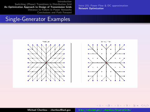
Network Optimization: Losses+Costs [J. Johnson, MC ’10]
Costs need to account for
“sizing lines” - grows with gab, linearly or faster (convex in g)
“breaking ground” - l0-norm (non convex in g) but also imposesdesired sparsity
Resulting Optimization is non-convex
ming>0
(tr
((G (g)
)−1
P
)+∑{a,b}
(αabgab + βabφγ(gab))
), φγ(x)= x
x+γ
Tricks (for efficient solution of the non-convex problem)
“annealing”: start from large (convex) γ and track to γ → 0(combinatorial)
Majorization-minimization (from Candes, Boyd ’05) for current γ:
g t+1 = argming>0
(tr(L) + α. ∗ g + β. ∗ φ′γ(g t
ab). ∗ gab
)Michael Chertkov – [email protected] http://cnls.lanl.gov/∼chertkov/SmarterGrids/
IntroductionSwitching (Phase) Transitions in Distribution Grid
An Optimization Approach to Design of Transmission GridsDistance to Failure in Power Networks
Conclusions and Path Forward
Intro (II): Power Flow & DC approximationNetwork Optimization
Single-Generator Examples
Michael Chertkov – [email protected] http://cnls.lanl.gov/∼chertkov/SmarterGrids/

IntroductionSwitching (Phase) Transitions in Distribution Grid
An Optimization Approach to Design of Transmission GridsDistance to Failure in Power Networks
Conclusions and Path Forward
Intro (II): Power Flow & DC approximationNetwork Optimization
Multi-Generator Example
Michael Chertkov – [email protected] http://cnls.lanl.gov/∼chertkov/SmarterGrids/

IntroductionSwitching (Phase) Transitions in Distribution Grid
An Optimization Approach to Design of Transmission GridsDistance to Failure in Power Networks
Conclusions and Path Forward
Intro (II): Power Flow & DC approximationNetwork Optimization
Adding Robustness
To impose the requirement that the network design should berobust to failures of lines or generators, we use the worst-casepower dissipation:
L\k (g) = max∀{a,b}:zab∈{0,1}|
∑{a,b} zab=N−k
L(z . ∗ g))
It is tractable to compute only for small values of k .
Note, the point-wise maximum over a collection of convexfunction is convex.
So the linearized problem is again a convex optimizationproblem at every step continuation/MM procedure.
Michael Chertkov – [email protected] http://cnls.lanl.gov/∼chertkov/SmarterGrids/

IntroductionSwitching (Phase) Transitions in Distribution Grid
An Optimization Approach to Design of Transmission GridsDistance to Failure in Power Networks
Conclusions and Path Forward
Intro (II): Power Flow & DC approximationNetwork Optimization
Single-Generator Examples
Michael Chertkov – [email protected] http://cnls.lanl.gov/∼chertkov/SmarterGrids/

IntroductionSwitching (Phase) Transitions in Distribution Grid
An Optimization Approach to Design of Transmission GridsDistance to Failure in Power Networks
Conclusions and Path Forward
Intro (II): Power Flow & DC approximationNetwork Optimization
Multi-Generator Example
Michael Chertkov – [email protected] http://cnls.lanl.gov/∼chertkov/SmarterGrids/

IntroductionSwitching (Phase) Transitions in Distribution Grid
An Optimization Approach to Design of Transmission GridsDistance to Failure in Power Networks
Conclusions and Path Forward
Intro (II): Power Flow & DC approximationNetwork Optimization
Conclusion (for the Network Optimization part)
A promising heuristic approach to design of power transmissionnetworks. However, cannot guarantee global optimum.
Submitted to CDC10: http://arxiv.org/abs/1004.2285
Future Work:
Bounding optimality gap?
Use non-convex continuation approach to place generators
possibly useful for graph partitioning problems
adding further constraints (e.g. don’t overload lines)
extension to (exact) AC power flow?
Michael Chertkov – [email protected] http://cnls.lanl.gov/∼chertkov/SmarterGrids/

IntroductionSwitching (Phase) Transitions in Distribution Grid
An Optimization Approach to Design of Transmission GridsDistance to Failure in Power Networks
Conclusions and Path Forward
Model of Load SheddingError Surface & Instantons
Outline
1 Introduction
2 Switching (Phase) Transitions in Distribution GridRedundancy & SwitchingSAT/UNSAT Transition & Message Passing
3 An Optimization Approach to Design of Transmission GridsIntro (II): Power Flow & DC approximationNetwork Optimization
4 Distance to Failure in Power NetworksModel of Load SheddingError Surface & Instantons
5 Conclusions and Path Forward
Michael Chertkov – [email protected] http://cnls.lanl.gov/∼chertkov/SmarterGrids/

IntroductionSwitching (Phase) Transitions in Distribution Grid
An Optimization Approach to Design of Transmission GridsDistance to Failure in Power Networks
Conclusions and Path Forward
Model of Load SheddingError Surface & Instantons
Normally the grid is ok (SAT) ... but sometimes failures(UNSAT) happens
How to estimate a probability of a failure?
How to predict (anticipate and hopefully) prevent the systemfrom going towards a failure?
Phase space of possibilities is huge (finding the needle in thehaystack)
Instanton
Generation
Load
84
Instanton 2
Michael Chertkov – [email protected] http://cnls.lanl.gov/∼chertkov/SmarterGrids/

IntroductionSwitching (Phase) Transitions in Distribution Grid
An Optimization Approach to Design of Transmission GridsDistance to Failure in Power Networks
Conclusions and Path Forward
Model of Load SheddingError Surface & Instantons
Model of Load Shedding [MC, F.Pan & M.Stepanov ’10]
Minimize Load Shedding = Linear Programming for DC
LPDC (d|G; x; u; P) = minf,ϕ,p,s
∑a∈Gd
sa
COND(f,ϕ,p,d,s|G;x;u;P)
COND = CONDflow ∪ CONDDC ∪ CONDedge ∪ CONDpower ∪ CONDover
CONDflow =
∀a :∑b∼a
fab =
{ pa, a ∈ Gp
−da + sa, a ∈ Gd
0, a ∈ G0 \ (Gp ∪ Gd )
)
CONDDC =
(∀{a, b} : ϕa−ϕb +xabfab =0
), CONDedge =
(∀{a, b} : −uab≤ fab≤uab
)
CONDpower =
(∀a : 0 ≤ pa ≤ Pa
), CONDover =
(∀a : 0 ≤ sa ≤ da
)
ϕ -phases; f -power flows through edges; x - inductances of edges
Michael Chertkov – [email protected] http://cnls.lanl.gov/∼chertkov/SmarterGrids/

IntroductionSwitching (Phase) Transitions in Distribution Grid
An Optimization Approach to Design of Transmission GridsDistance to Failure in Power Networks
Conclusions and Path Forward
Model of Load SheddingError Surface & Instantons
SAT/UNSAT & Error SurfaceStatistics of Loads
P(d|D; c) ∝ exp(− 1
2c
∑i
(di−Di )2
D2i
)D is the normal operational position in the space of demands
Instantons (special instances of demands from the error surface)
Points on the error-surface maximizing P(d|D; c) - locally!
arg maxd P(d)|LPDC (d)>0 - most probable instanton
The maximization is not concave (multiple instantons)
No Shedding (SAT) - Boundary - Shedding (UNSAT) = Error Surface
The task: to find the most probable failure modes [instantons]
Michael Chertkov – [email protected] http://cnls.lanl.gov/∼chertkov/SmarterGrids/

IntroductionSwitching (Phase) Transitions in Distribution Grid
An Optimization Approach to Design of Transmission GridsDistance to Failure in Power Networks
Conclusions and Path Forward
Model of Load SheddingError Surface & Instantons
Instanton Search Algorithm [Sampling]
Borrowed (with modifications) from Error-Correction studies:analysis of error-floor [MC, M.Stepanov, et al ’04-’10]
Construct Q(d) ={P(d), LPDC (d) > 0
0 , LPDC (d) = 0
Generate a simplex (N+1points) of UNSAT points
Use Amoeba-Simplex[Numerical Recepies] tomaximize Q(d)
Repeat multiple times(sampling the space ofinstantons)
Point at the Error Surfaceclosest to normal operational point
@@
@@
normal operational point
demand1
demand2
demand...
Error Surface �����
load sheddingload sheddingload shedding
no load sheddingno load sheddingno load shedding
Michael Chertkov – [email protected] http://cnls.lanl.gov/∼chertkov/SmarterGrids/

IntroductionSwitching (Phase) Transitions in Distribution Grid
An Optimization Approach to Design of Transmission GridsDistance to Failure in Power Networks
Conclusions and Path Forward
Model of Load SheddingError Surface & Instantons
Example of Guam [MC, F.Pan & M.Stepanov ’10]
0
1
2
3
4
5
6
7
8
9
23 33 43 53 63 73 83 93 103
Ave
rage
Lo
ad (
D)
Bus ID
Instanton 1
Instanton 2
Instanton 3
0
0.005
0.01
0.015
0.02
0.025
0 3 6 9 12 15 18 21 24 27 30 33 36 39 42 45 48 51 54 57 60 63 66 69 72 75 78 81 84 87 90 93 96
Inst
anto
nV
alu
e(-
log(
P(d
))/T
)
Run ID
Load
Generator
Instanton 1
Instanton 3
Instanton 2
Common
The instantons are sparse (localized ontroubled nodes)
The troubled nodes are repetitive inmultiple-instantons
Instanton structure is not sensitive tosmall changes in D and statistics ofdemands
Michael Chertkov – [email protected] http://cnls.lanl.gov/∼chertkov/SmarterGrids/

IntroductionSwitching (Phase) Transitions in Distribution Grid
An Optimization Approach to Design of Transmission GridsDistance to Failure in Power Networks
Conclusions and Path Forward
Model of Load SheddingError Surface & Instantons
Example of IEEE RTS96 system [MC, F.Pan & M.Stepanov ’10]
0
50
100
150
200
250
0 10 20 30 40 50 60 70
Ave
rage
De
man
d (
D)
Bus ID
14.5
19.5
24.5
29.5
34.5
39.5
44.5
49.5
0 2 4 6 8 10 12 14 16 18 20 22 24 26 28 30 32 34 36 38 40 42 44 46 48
Inst
anto
n V
alu
e (
-lo
g(P
(d))
/T)
Run IDIn
sta
nto
n1
Ins
tan
ton
2
Ins
tan
ton
3
0
1
2
3
4
5
6
0 10 20 30 40 50 60 70
d/D
Bus ID
Instanton1
Instanton2
Instanton3
Load
Generator
Instanton 1
Instanton 3
Instanton 2
The instantons are well localized (but stillnot sparse)
The troubled nodes and structures arerepetitive in multiple-instantons
Instanton structure is not sensitive tosmall changes in D and statistics ofdemands
Michael Chertkov – [email protected] http://cnls.lanl.gov/∼chertkov/SmarterGrids/

IntroductionSwitching (Phase) Transitions in Distribution Grid
An Optimization Approach to Design of Transmission GridsDistance to Failure in Power Networks
Conclusions and Path Forward
Model of Load SheddingError Surface & Instantons
Concusions and Path Forward (for the distance to failure)Conclusions
Formulated Load Shedding (SAT/UNSAT condition) as an LPDC
Posed the problem of the Error-Surface and Instantons descriptionin the power-grid setting
Instanton-amoeba algorithm was suggested and tested on examples
Path Forward
The instanton-amoeba allows upgrade to other (than LPDC )network stability testers, e.g. for AC flows and transients
Instanton-search can be accelerated, utilizing LP-structure of thetester (in the spirit of [MC,MS ’08])
This is an important first step towards exploration of “next level”problems in power grid, e.g. on interdiction [Bienstock et. al ’09],optimal switching [Oren et al ’08], cascading outages [Dobson et al’06], and control of the extreme [outages] [Ilic et al ’05]
Michael Chertkov – [email protected] http://cnls.lanl.gov/∼chertkov/SmarterGrids/

IntroductionSwitching (Phase) Transitions in Distribution Grid
An Optimization Approach to Design of Transmission GridsDistance to Failure in Power Networks
Conclusions and Path Forward
Bottom Line
A lot of interesting power grid settings for CS/IT, Physics analysis
The research is timely (blackouts, renewables, stimulus)
Stay tuned ... the field is growing explosively
Other Problems under investigation by the team
Control of Reactive Power Flow in a radial circuit [K. Turtisyn, P.Sulc, S. Backhaus, MC ’09 = arXiv:0912.3281 + selected for SuperSession of IEEE/PES Gen Mtg 2010]
Efficient PHEV charging via queuing/scheduling with and withoutcommunications and delays [S. Backhaus, MC, K. Turitsyn, N.Sinitsyn]
For more info - check:
http://cnls.lanl.gov/~chertkov/SmarterGrids/Michael Chertkov – [email protected] http://cnls.lanl.gov/∼chertkov/SmarterGrids/

IntroductionSwitching (Phase) Transitions in Distribution Grid
An Optimization Approach to Design of Transmission GridsDistance to Failure in Power Networks
Conclusions and Path Forward
Thank You!Michael Chertkov – [email protected] http://cnls.lanl.gov/∼chertkov/SmarterGrids/

The Switching Story with Renewables
Switching/control with renewables (I)
Fraction 1/3 of consumers produce amount zEvery consumer consumes random number in (0.9,1.1)
0
0.2
0.4
0.6
0.8
1
1.2
0 0.5 1 1.5 2
firm generation per customer, y/D
renewable generation capability, z
D=3, x=1, !=0.2, f=1/3
R=0,R=1R=2R=3
Example n. 1# producers
M →∞
# consumersN = 3M
y/3 = 1− z/3
generation > consumption
y/3 = 1.1
somebody must serve D-R+1 fully demanding consumers
Main Switching Story
Michael Chertkov – [email protected] http://cnls.lanl.gov/∼chertkov/SmarterGrids/

The Switching Story with Renewables
Switching/control with renewables (II)
Example n. 2
0
0.2
0.4
0.6
0.8
1
1.2
0 0.2 0.4 0.6 0.8 1firm generation per customer, y/D
avg. renewables per customer, z/2
D=3, x=1, !=0.2
R=0, R=1R=2R=3
Every consumer produced a random number between (0,z)
Main Switching Story
Michael Chertkov – [email protected] http://cnls.lanl.gov/∼chertkov/SmarterGrids/

The Switching Story with Renewables
Switching/control with renewables (III)
Example n. 3
0
0.2
0.4
0.6
0.8
1
1.2
0 0.2 0.4 0.6 0.8 1
firm generation per customer, y/D
coverage of renewables, f
D=3, R=3, x=1, !=0.2
z=0.5
z=1.0
z=2.0
amount z is produced by fraction f of consumers
produced > consumed
y/3 > 1− fz
Main Switching Story
Michael Chertkov – [email protected] http://cnls.lanl.gov/∼chertkov/SmarterGrids/


![@let@token eserved@d = *@let@token height=.55in]figures ...sorensen/Talks/MTNS08/MTNS08T.pdf · Lyapunov Equations for system Gramians AP+PAT +BBT = 0 ATQ+QA+CTC = 0 With P= Q= S](https://img.pdfslide.us/doc/110x75/5f64344bb0527558f94f4a16/lettoken-eservedd-lettoken-height55infigures-sorensentalksmtns08.jpg)