To the Graduate Council: I am submitting herewith a thesis written by Vitaliy Leonidovich Orekhov entitled “A Full Scale Camera Calibration Technique with Automatic Model Selection – Extension and Validation” I have examined the final electronic copy of this thesis for form and content and recommend that it be accepted in partial fulfillment of the requirements for the degree of Master of Science, with a major in Electrical Engineering.

Mongi A. Abidi Major Professor

We have read this thesis and recommend its acceptance: Besma Roui Abidi Michael J. Roberts Accepted for the Council:

Carolyn R. Hodges Vice Provost and Dean of the Graduate School

(Original signatures are on file with official student records.)

A FULL SCALE CAMERA CALIBRATION TECHNIQUE WITH AUTOMATIC MODEL SELECTION –

EXTENSION AND VALIDATION

A Thesis

Presented for the

Master of Science

Degree

University of Tennessee, Knoxville

Vitaliy Leonidovich Orekhov August 2007

ii

ACKNOWLEDGEMENTS First of all I would like to thank my parents for raising me to be the person I am today. I am thankful to them for helping me shape my values and goals and most of all instilling in a desire to know the Truth and love of God. I would like to thank my advisor Dr. Mongi A. Abidi for his academic and financial support throughout my time at the University of Tennessee. I am grateful to Dr. Besma Abidi for guiding me in the research and for the patience while working with me. Thank you also to Dr. Michael J. Roberts for serving on my graduate committee. I also would like to thank the entire IRIS lab including Dr. Andreas Koschan, Dr. David Page, the research staff, and all of the students. I appreciate the valuable feedback and interactive discussion at the research meetings.

iii

ABSTRACT This thesis presents work on the testing and development of a complete camera calibration approach which can be applied to a wide range of cameras equipped with normal, wide-angle, fish-eye, or telephoto lenses. The full scale calibration approach estimates all of the intrinsic and extrinsic parameters. The calibration procedure is simple and does not require prior knowledge of any parameters. The method uses a simple planar calibration pattern. Closed-form estimates for the intrinsic and extrinsic parameters are computed followed by nonlinear optimization. Polynomial functions are used to describe the lens projection instead of the commonly used radial model. Statistical information criteria are used to automatically determine the complexity of the lens distortion model.

In the first stage experiments were performed to verify and compare the performance of the calibration method. Experiments were performed on a wide range of lenses. Synthetic data was used to simulate real data and validate the performance. Synthetic data was also used to validate the performance of the distortion model selection which uses Information Theoretic Criterion (AIC) to automatically select the complexity of the distortion model.

In the second stage work was done to develop an improved calibration procedure which addresses shortcomings of previously developed method. Experiments on the previous method revealed that the estimation of the principal point during calibration was erroneous for lenses with a large focal length. To address this issue the calibration method was modified to include additional methods to accurately estimate the principal point in the initial stages of the calibration procedure. The modified procedure can now be used to calibrate a wide spectrum of imaging systems including telephoto and veri-focal lenses.

Survey of current work revealed a vast amount of research concentrating on calibrating only the distortion of the camera. In these methods researchers propose methods to calibrate only the distortion parameters and suggest using other popular methods to find the remaining camera parameters. Using this proposed methodology we apply distortion calibration to our methods to separate the estimation of distortion parameters. We show and compare the results with the original method on a wide range of imaging systems.

iv

TABLE OF CONTENTS LIST OF TABLES ..................................................................................................................................... VI LIST OF FIGURES ..................................................................................................................................VII LIST OF FIGURES ..................................................................................................................................VII 1 INTRODUCTION ...............................................................................................................................1

1.1 MOTIVATION.................................................................................................................................2 1.2 CONTRIBUTIONS............................................................................................................................3 1.3 ORGANIZATION.............................................................................................................................4

2 LITERATURE REVIEW ...................................................................................................................5 2.1 CAMERA MODELS .........................................................................................................................5

2.1.1 Pinhole Camera Model .............................................................................................. 5 2.1.2 Wide-Angle and Omnidirectional Camera Models .................................................... 8 2.1.3 Lens Projections....................................................................................................... 10 2.1.4 Radial Distortion...................................................................................................... 14

2.2 GENERAL CALIBRATION .............................................................................................................19 2.2.1 Test-Range Calibration............................................................................................ 19 2.2.2 Non-metric Calibration............................................................................................ 23 2.2.3 Self-Calibration........................................................................................................ 24

2.3 WIDE-ANGLE DISTORTION CALIBRATION...................................................................................27 2.3.1 Line Based Calibration ............................................................................................ 28

2.3.1.1 Extracting Lines and Edges .................................................................. 29 2.3.1.2 Extracting Distortion Parameters from Lines ....................................... 30

2.3.2 Point Correspondence Distortion Calibration......................................................... 32 2.3.3 Distortion Calibration Summary.............................................................................. 38

2.4 TELEPHOTO AND ZOOM LENS CALIBRATION ..............................................................................38 2.5 LITERATURE REVIEW SUMMARY ................................................................................................45

3 ASSESSMENT AND VALIDATION OF INITIAL IMPLEMENTATION ................................47 3.1 CALIBRATION METHOD FRAMEWORK.........................................................................................47

3.1.1 The Closed-form Solution ........................................................................................ 48 3.1.2 Solving for Distortion............................................................................................... 48 3.1.3 Final Parameter Optimization ................................................................................. 49 3.1.4 Distortion Model Selection ...................................................................................... 50

3.2 EVALUATION OF DISTORTION MODEL COMPLEXITY SELECTION ................................................53 3.2.1 Validating Model Selection Results with Synthetic Data ......................................... 54 3.2.2 Model Selection Results with Real Data .................................................................. 55 3.2.3 Which criteria should be used?................................................................................ 55

3.3 STANDARD LENS CALIBRATION RESULTS...................................................................................58 3.4 TELE-PHOTO LENS CALIBRATION RESULTS ................................................................................61

3.4.1 Synthetic Data of Tele-photo Lens ........................................................................... 61 3.4.2 Real Data of Tamron 300mm Lens .......................................................................... 63 3.4.3 Nikon 70-210mm varifocal lens calibration............................................................. 66

3.5 RESULTS WITH DIFFERENT INITIALIZATION VALUES OF PRINCIPAL POINT .................................75 3.5.1 Finding the Center of Expansion ............................................................................. 75 3.5.2 Experimental Results of the Principal Point Initialization ...................................... 77

4 IMPROVED COMPLETE CAMERA CALIBRATION ...............................................................83

v

4.1 MOTIVATION...............................................................................................................................83 4.2 MODELING DISTORTION..............................................................................................................83 4.3 OPTIMIZING DISTORTION ONLY..................................................................................................86 4.4 STRAIGHT LINE METHOD FOR DISTORTION CALIBRATION..........................................................88

4.4.1 SLM Procedure ........................................................................................................ 88 4.4.2 Experimental Results with SLM Distortion Calibration .......................................... 90 4.4.3 Experiments with the Reversed Distortion Model Required for SLM ...................... 92 4.4.4 Discussion of SLM Distortion Calibration............................................................... 95

4.5 FUTURE WORK WITH THE PROPOSED CALIBRATION METHOD ....................................................95 5 REAL-TIME DISTORTION CORRECTION................................................................................96

5.1 CAMERA SET UP .........................................................................................................................96 5.2 CAMERA CALIBRATION...............................................................................................................97 5.3 IMAGE CAPTURE AND CORRECTION............................................................................................98 5.4 ANALYSIS AND COMPARISON OF FRAME RATES .........................................................................99

6 CONCLUSIONS ..............................................................................................................................101 6.1 SUMMARY.................................................................................................................................101 6.2 CONTRIBUTIONS........................................................................................................................101 6.3 FUTURE WORK..........................................................................................................................101

REFERENCES..........................................................................................................................................103 VITA...........................................................................................................................................................112

vi

LIST OF TABLES Table 2.1. Variable-parameter range of Shih’s zoom camera [Shih98]. .......................... 41 Table 3.1. Commonly used types of lens projections. ...................................................... 49 Table 3.2. Model selection criteria. .................................................................................. 52 Table 3.3. Model complexity selection accuracy using synthetic data............................. 54 Table 3.4. Complexity selection of RDDD model using real data. .................................. 56 Table 3.5. Complexity selection of LPDD model using real data. ................................... 56 Table 3.6. LPDD distortion model complexity selection for Nikon 50mm lens. ............. 58 Table 3.7. Calibration results for standard Nikon 50mm lens. ......................................... 59 Table 3.8. Results for synthetic data with RDDD model. ................................................ 62 Table 3.9. Results for synthetic data with LPDD model. ................................................. 63 Table 3.10. Results for synthetic telephoto data with RDDD model................................ 63 Table 3.11. Results for synthetic telephoto data with LPDD model. ............................... 63 Table 3.12. Calibration results for Tamron 300mm lens with different aperture settings.64 Table 3.13. Reprojection error for Tamron 28-300mm lens............................................. 64 Table 3.14. Effective focal length estimates for Tamron 28-300mm lens........................ 65 Table 3.15. Error measurements for varifocal Nikon Nikkor 70-210 mm lens calibration............................................................................................................................................ 67 Table 3.16. Focal Length for Varifocal Nikon Nikkor 70-210mm Lens Calibration....... 68 Table 3.17. Principal point location for varifocal Nikon NIkkor 70-210mm lens. .......... 70 Table 3.18. Distance in pixels that the principal point is away from the actual image center for Nikon 70-210mm lens. ..................................................................................... 71 Table 3.19. Calibration results with varied initialization values for principal point with LPDD model. .................................................................................................................... 78 Table 3.20. Calibration results with varied initialization values for principal point with RDDD model. ................................................................................................................... 78 Table 3.21. Calibration results with varied initialization value for principal point. ......... 79 Table 3.22. Comparison of Nikon 210-70mm lens MSE reprojection error. ................... 80 Table 3.23. Nikon 210mm calibration results with initialized principal point to image center................................................................................................................................. 80 Table 4.1. RDDD model selection for wide angle lens with and without optimization. .. 85 Table 4.2. LPDD model selection for wide angle lens with and without optimization.... 85 Table 4.3. Complexity selection of RDDD model with optimized distortion only. ......... 87 Table 4.4. Complexity selection of LPDD model with optimized distortion only. .......... 87 Table 4.5. MSE of original method and with optimized distortion for RDDD. ............... 87 Table 4.6. MSE of previous method and with optimized distortion for LPDD................ 87 Table 4.7. Computation time of entire calibration process with original and SLM calibration methods. .......................................................................................................... 90 Table 4.8. MSE deviations from LSLF using original and SLM calibration methods. .... 92 Table 4.9. Complexity selection of RDDD model using real data with SLM. ................. 92 Table 4.10. MSE for real data with original and reversed RDDD distortion model. ....... 93 Table 4.11. MSE for real data with original and reversed LPDD distortion model. ........ 93 Table 5.1. Frame rates comparison for real-time distortion correction. ......................... 100

vii

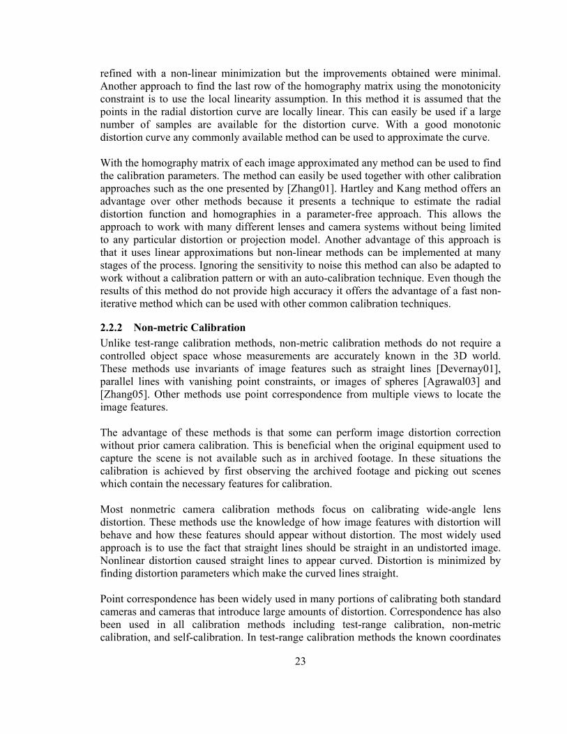
LIST OF FIGURES Figure 2.1: Perspective projection in pinhole camera model.............................................. 6 Figure 2.2: Geometry to map points on the image.............................................................. 7 Figure 2.3: Projection of scene point onto a finite image plane found in a fish-eye lens... 9 Figure 2.4: Geometry of ideal lens projections................................................................. 10 Figure 2.5: Projection of Perspective lens model. ............................................................ 11 Figure 2.6: Equidistance projection. ................................................................................. 12 Figure 2.7: Lens projections where A is the perspective projection, B is the stereographic projection, C is the equidistant projection, D is the equisolid angle projection, and E is the orthogonal projection. ....................................................................................................... 13 Figure 2.8: Two types of radial distortion. The original undistorted rectangle, represented by dashed lines, is shown with the presence of (a) barrel distortion (blue) and (b) pincushion distortion (red)................................................................................................ 14 Figure 2.9: Displacement of original point due to radial and tangential lens distortion... 15 Figure 2.10: Mapping of straight edges in perspective image (a) to curves in fisheye image (b) as result of radial distortion. ............................................................................. 16 Figure 2.11: Distortion causes point M to be mapped to dm instead of m . ................... 16 Figure 2.12: Effect of radial distortion on 3D lines joining sets of corresponding points for (a) no distortion, (b) pin-cushion distortion, and (c) radial distortion [Tordoff04]. ... 25 Figure 2.13: Erroneous data extracted from a distorted image. Line segments which should be individual lines were linked together [Ahmed05]. ........................................... 30 Figure 2.14: Least square approximation for distortion error measurement. ................... 31 Figure 2.15: Sample calibration pattern with extracted control points............................. 33 Figure 2.16: 1D radial camera model diagram. ................................................................ 36 Figure 2.17: Plane projection from lines in 1D Radial Camera........................................ 37 Figure 2.18: Nikon 200-400mm telephoto lens (www.dpreview.com). ............................ 39 Figure 2.19: Canon NU-700 Pan-Tilt head with 20x (4.2-84mm) zoom lens www.canon.ca................................................................................................................... 40 Figure 2.20: Variation in X (a) and Y (b) coordinates of an autocollimated laser image with varied zoom and focus settings [Willson94]............................................................. 42 Figure 2.21: Variation in Cx (a) and Cy (b) coordinates of the principal point with varied zoom and focus settings [Willson94]................................................................................ 42 Figure 2.22: Final adjusted model for Cx (a) and Cy (b) coordinates of the principal point with varied zoom and focus settings [Willson94]............................................................. 43 Figure 2.23: Calibration pattern with focal length of 70mm (a) and 210mm (b) with Nikon 210mm Lens at 3m focus....................................................................................... 44 Figure 2.24: Complete calibration pattern (a) with images captured at wide-angle setting (b) and telephoto setting (c). ............................................................................................. 46 Figure 3.1: Computation time for Zhang’s data using the lens projection model. Plot shows the computation time as the number of radial and tangential coefficients are changed on a 640x480 image............................................................................................ 51 Figure 3.2: Distortion model complexity selection with the MDL criterion. (a) shows the complete model complexity, (b) shows the complexities with only radial coefficients, and (c) shows the complexity due to each type of distortion coefficient. ............................... 56

viii

Figure 3.3: Nikon Nikkor 50mm f/1.4D AF lens www.nikonusa.com............................. 58 Figure 3.4: Principal point location using our calibration method for Nikon 50mm lens with varied focus setting. .................................................................................................. 60 Figure 3.5: Principal point location using OpenCV calibration method for Nikon 50mm lens with varied focus setting............................................................................................ 60 Figure 3.6: Synthetic data with and without pin-cushion distortion................................. 61 Figure 3.7: Plots of original synthetic data (a), reprojected image points using RDDD (b), and plot of both data sets in same image (c). .................................................................... 62 Figure 3.8: Tamron 300mm principal point location with varied focal length settings using our implementation. ................................................................................................ 65 Figure 3.9: Tamron 300mm principal point location with varied focal length settings using OpenCV implementation......................................................................................... 65 Figure 3.10: Collection of images captured at different focal length and focus setting with the Nikon 70-210mm lens................................................................................................. 66 Figure 3.11: Mean square error for Nikon 210mm lens for different focal length and focus settings..................................................................................................................... 68 Figure 3.12: Focal length estimate for the Nikon 210mm lens with different focal length and focus settings. (a) shows the 3D diagram with the lens focus and focal length settings and (b) shows the side profile of the actual and estimated focal length of the lens.......... 69 Figure 3.13: Principal point location with fixed focal length and varied focus................ 71 Figure 3.14: Principal point location with fixed focus and varied focal length................ 72 Figure 3.15: 3D plot of principal point location with varied focal length settings........... 72 Figure 3.16: Distance between principal point and image center for Nikon 210mm lens.72 Figure 3.17: Distance between distortion center and image center for Nikon 210mm lens............................................................................................................................................ 73 Figure 3.18: Distortion center position on an image plane of the Nikon 210mm lens with different focus settings and focal lengths represented by the line segments. (a) shows the 3D diagram with the lens focus and focal length settings and (b) shows the top profile as seen on the image plane. ................................................................................................... 74 Figure 3.19: Calibrating pattern of Nikon 210mm lens at focal length of 210mm and focused at a distance of three meters from the pattern...................................................... 74 Figure 3.20: Images with different zoom showing calibration pattern at 50mm (a) and 70mm (b). The center of expansion can be estimated by drawing lines connecting corresponding points and finding the intersection of the lines. ........................................ 76 Figure 3.21: Lines connecting corresponding points from two images of different zoom (50mm and 70mm) (a). Close up view of the intersection of lines at the image center of expansion (b)..................................................................................................................... 77 Figure 3.22: Focal length estimate with initialized principal point to image center for the Nikon 210mm lens. (a) shows the 3D diagram with varied lens focus and focal length settings and (b) shows the side profile of the actual and estimated focal length of the lens............................................................................................................................................ 81 Figure 3.23: Nikon 210mm principal point location after optimization with initialization at the image center. (a) shows the 3D diagram with the lens focus and focal length settings and (b) shows the top profile as seen on the image plane. .................................. 81 Figure 4.1: Initial implementation of the calibration method. .......................................... 84

ix

Figure 4.2: New improved calibration method. ................................................................ 84 Figure 4.3: The original distorted image (a) and image showing distorted lines used for the SLM distortion calibration (b). ................................................................................... 89 Figure 4.4: Image distortion correction on real images with SLM................................... 91 Figure 4.5: Comparison of MSE calibration with original RDDD and reversed RDDD models. .............................................................................................................................. 94 Figure 4.6: Comparison of MSE calibration with original LPDD and modified LPDD models. .............................................................................................................................. 94 Figure 4.7: Calibration MSE with reversed models using LPDD and RDDD. ................ 95 Figure 5.1: Diagram of camera calibration and real time distortion correction................ 97 Figure 5.2: Simple calibration pattern used for camera calibration.................................. 98 Figure 5.3: Extracted corners from the calibration Pattern. Blue crosses represent selected points and the red crosses represent outliers..................................................................... 98 Figure 5.4: GUI for correcting distortion on an image sequence in real time. ................ 99 Figure 5.5: Sample of original and corrected images from image sequence. Figures (a) and (b) show distorted and corrected image for 185º fish-eye image and image(c) and (d) show distorted and corrected images for 80º wide angle image..................................... 100

1

1 INTRODUCTION In computer vision applications camera calibration is an essential step in quantitative image analysis. To extract metric information from images it is necessary to understand how a point in the scene is projected onto the image sensor. In essence the goal of camera calibration is to identify the camera model which accurately describes how objects in the 3D world are projected onto the 2D image sensor. We have a great number of camera models and procedures available today to calibrate a camera but the challenge is in choosing the model and procedure which are both simple and provide accurate results. Some of the first computer vision calibration methods were derived from methods used by the photogrammetric community. Due to the complexity of the calibration procedures and advances in the use of computers for analytical analysis, simpler methods have been developed which are now widely used in the computer vision community [Heikkila97, Lenz87, Tsai87, Zhang00]. The most popular calibration methods take several images of a known calibration object from different camera positions. The projection of calibration object’s features onto the image sensor is approximated with the pinhole camera model. The deviation of features due to lens distortion, from the pinhole camera is modeled with radial and tangential distortions [Heikkila00, Heikkila97, Lenz87, Tsai87, Zhang00]. Most of these methods either require prior knowledge of some camera parameters or are restricted to normal cameras with perspective projections. As a result these methods can not be used on cameras where prior knowledge of some parameters is not known or on camera systems which are equipped with wide-angle or fish-eye lenses. Cameras with wide-angle and fish-eye lenses exhibit significant amount of lens distortion which must be given special consideration. Much research has been made in the area of distortion calibration on wide-angle and fish-eye lenses [Hartley05, Sagawa05, Graf05, Kang01, Kannala06, Devernay01, Ahmed05, Stein97, Thirthala05b]. Many of these methods use calibration patterns [Hartley05, Segawa05, Graf05], while other nonmetric methods depend on the presence of certain features in the scene [El-Melegy03, Basu95, Devernay01, Swaminathan00, Kang01]. The limitation of most of these methods is that they are concerned with only correcting the distortion while leaving the rest of the intrinsic and extrinsic parameters to be estimated with other methods. Of all the proposed distortion calibration methods few address the issues of a generic distortion model which could work on a wide range of cameras while only [El-Melegy03, Kinoshita00, Wei98] consider an automatic distortion model selection method. The common radial distortion polynomial does not work well with large distortions where lenses do not exactly follow the lens projection models. Hartley and Kang [Hartley05] presented a parameter-free method to model distortion which does not rely on any

2

particular distortion model and as a result can be used on fish-eye, wide angle, and normal angle lenses. However, as the authors point out, the distortion curve must eventually be approximated by specific techniques to be useful for image correction. The number of methods which focus on complete generic calibration is limited. In [Kannala06] a complete method is presented for fish-eye lenses, which is also suitable for normal and wide-angle lenses. The authors assume knowledge of nominal focal length and angle of view for initialization of internal parameters. In [Ramalingam05] another generic camera calibration approach is described which proposes to use a non-parametric association of a projection ray in 3D to every pixel in an image. Here we present the development of a unified framework for a full scale camera calibration technique which addresses some shortcomings of previous methods. The calibration procedure is an extension and improvement of previous work by Christopher Broadus [Broaddus05]. By exploring recent advances in the area of camera calibration and testing the performance of the previously developed method we have identified and addressed areas which can be improved. The result is a complete generic calibration procedure with distortion model complexity selection which can be applied to normal, telephoto, wide-angle, and fish-eye lenses.

1.1 Motivation The starting point and initial motivation for this work comes from previous work done on camera calibration in the Imaging, Robotics, and Intelligent Systems (IRIS) laboratory. The previously developed calibration method was tested on several real and synthetic data sets but lacked results for lenses with large focal lengths. The performance of this method also needed to be verified with synthetic data and compared to other methods. Additional motivation comes from reviewing literature on current advances in the area of camera calibration. As was mentioned previously some limitations of most proposed methods are that they are either not complete calibration methods or they lack the ability to be used with a wide range of imaging systems. For a calibration method to be complete we need to be able to find all of the intrinsic and extrinsic parameters which also include the distortion parameters. With a complete calibration method we are not required to make demanding assumptions of camera parameters if they are not available. If some parameters are known they can always be included to reduce the computational complexity. Since some methods require prior knowledge of some camera parameters they can not be used when these parameters are unknown. This limits the ability of these methods to be used with a wide range of camera systems. Another concern with calibration is the need to accurately model lens distortion. The distortion can range from very minimal in normal lenses to large distortion found in wide-angle lenses and fish-eye lenses. To be able to model all of the different degrees of distortions, a model is necessary which can accurately and efficiently estimate the distortion in a broad range. In

3

the event that several models can model the distortion it is necessary to have quantitative measure criteria to automatically select the best distortion model. From these motivations we want a complete calibration method which can accurately model all of the camera parameters without assuming any known parameters. It is also desired to be able to efficiently and accurately model distortion which is found in wide-angle and fish-eye lenses. With the distortion model we want to retain the ability to automatically select the best and least complex distortion model from among competing models.

1.2 Contributions Contributions include:

• Testing and comparing the original calibration method o Tested calibration performance on real and synthetic data of telephoto

lenses. o Verified and compared the successful selection of distortion model with

synthetic data for five different criteria. • Determined the limitations of the calibration procedure for telephoto lenses and

modified the previous method to accurately calibrate systems with large focal length.

• Proposed and presented a new calibration method which separates the estimation of the distortion parameters from the rest of the camera parameters in order to achieve faster calibration.

The first contribution of this thesis is the testing and evaluation of the previously developed camera calibration method [Broaduss05]. Previous camera calibration results were not shown for imaging systems with large focal lengths. We tested the performance of the calibration method on synthetic and real data from telephoto lenses. For real data the tests were performed on several vari-focal telephoto lenses which included Nikon Nikkor 70-300mm lens, Tamron 70-300mm lens, and Nikon Nikkor 60-210mm lens. To verify the calibration procedure the tests were also extended to normal Nikon Nikkor 50mm lens. In these experiments tests were performed on a wide range of focal length settings. In addition, the effects of changing the focus settings and aperture were examined. In [Broaduss05] automatic distortion model selection was performed using Information Theoretic Criterion (AIC). The performance of this method was shown on both synthetic and real data but nowhere was the accuracy of selection evaluated. Another contribution of this thesis is the validation of the automatic distortion model complexity selection using synthetic data. The experiment was performed with synthetic data generated with several competing distortion models and with random orientations and translations. Noise was added to the data to test the robustness of the model selection for all of the criteria.

4

With the test results of calibrating the telephoto lenses it was determined that the estimation of the principal point is incorrect for large focal lengths. To accurately estimate the principal point we explored several definitions of image center and added the ability to accurately estimate the distortion center and zoom of expansion separate from the rest of the calibration method. The previously used method was then modified to enable the use of these values in the calibration when calibration lenses with large focal lengths. The contribution in this area is a modified calibration method to accurately calibrate telephoto lenses. Results are shown for several different lenses with varying focal length and focus settings. The last contribution is the development of a new calibration method in which we propose to separate the estimation of the distortion model parameters from the rest of the camera parameters. Several possible techniques for the method were explored and some were implemented and compared to previous results. The new method offers the advantage of estimating the distortion parameters and distortion model before optimizing all of the camera parameters in bundle adjustment. This offers a significant decrease in computation time and a possibility to increase calibration accuracy.

1.3 Organization In this paper we study the current advances in camera calibration and introduce a new method based on results obtained from [Broaduss05]. In chapter 2 a survey and underlying theory is presented of recent advances in the area of camera calibration which consider lens distortion. In Chapter 3 we show the results for experiments performed with the method in [Broaduss05] and address some of its limitations. A new calibration method and the experimental results comparing it to other methods are shown in Chapter 4. Chapter 5 addresses implementations of the calibration method for real time distortion correction. Summary and conclusions are presented in Chapter 6.

5

2 LITERATURE REVIEW In this chapter, different approaches used to perform camera calibration will be introduced. Many calibration procedures are available in literature. With the exception of a few methods, each calibration method focused on calibrating a particular imaging system and as a result each approach has its own assumptions and technique. The main portion of the following survey will focus on calibrating distortion which is present in most imaging systems. The distortion becomes a significant cause of error in systems equipped with wide angle and omnidirectional lenses. The advantages of wide-viewing angle lenses are that they allow the camera to capture large scenes in a single image. Since non-linear lens distortion found in these lenses can account for significant errors, results from three-dimensional (3D) reconstructions and geometrical measurements may be inadequate for computer vision applications, particularly where a high degree of accuracy is required. Accurate reconstruction of these distorted scenes is the key to obtaining correct correspondences between the 3D world and the two-dimensional images. With accurate mathematical models of the camera and lens distortion parameters, reconstruction can be performed to correct the distortion in the images. This survey provides a review of research efforts into modeling and calibrating distortion found in cameras with wide angle lenses and other omnidirectional systems. Methods are examined which make an effort to separate the calibration of distortion and other camera parameters. These methods allow the correction of distortion in images without having to know all of the intrinsic camera parameters.

2.1 Camera Models

2.1.1 Pinhole Camera Model Mathematical models of cameras are required for analyzing and extracting information from images of the real world. Complex nonlinear distortions make this process very challenging and as a result many approaches to fix the problem have been presented. Traditional methods of modeling cameras begin with the basic pin-hole camera model which can be later expanded to other more complex models [Medioni05]. The pinhole camera model is shown in Figure 2.1. A point in three-dimensional space

( )T,, ZYX=M is projected onto the two-dimensional (2D) image plane to point ( )T,vum = . If the straight line formed by the projection of point M unto the image plane

is extended, it will pass through the optical center C (center of projection). The distance from the optical center to the image plane is the focal length ( f ). By using simple geometry (Figure 2.2) points on the image plane ),( vu can be expressed in terms of focal length and coordinates of M :

6

Image plane

C

f z

y

x

m

v

u

M

Figure 2.1: Perspective projection in pinhole camera model.

ZXfu = (1)

ZYfv = . (2)

The equations introduced above are non-linear but by using homogenous coordinates the pinhole camera model can be made into linear transformations. Homogenous coordinates are used in computer vision as a convenient way of representing the real 3D world and 2D image space by extending it to projective space [Hartley04].

Using homogeneous coordinates points m and M become ( )⎥⎥⎥

⎦

⎤

⎢⎢⎢

⎣

⎡⇒

1, v

uvu and

( )⎥⎥⎥⎥

⎦

⎤

⎢⎢⎢⎢

⎣

⎡

⇒

1

,,ZYX

ZYX , respectively. Given a coordinate in homogenous coordinates

),,,( kkZkYkX the original coordinates can be recovered by dividing by k to obtain ),,( ZYX .

The projection of point M onto point m on the image plane is represented by:

MPm = (3) where P is the projection matrix. The basic model of the pinhole camera using equation (3) and homogenous coordinates becomes

7

⎥⎥⎥⎥

⎦

⎤

⎢⎢⎢⎢

⎣

⎡

⎥⎥⎥

⎦

⎤

⎢⎢⎢

⎣

⎡=

⎥⎥⎥

⎦

⎤

⎢⎢⎢

⎣

⎡

10100000000

1ZYX

ff

vu

(4)

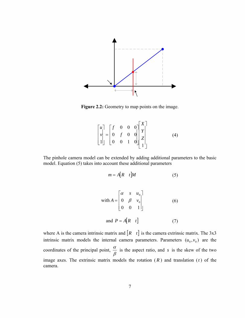
The pinhole camera model can be extended by adding additional parameters to the basic model. Equation (5) takes into account these additional parameters

[ ]MtRAm = (5)

with⎥⎥⎥

⎦

⎤

⎢⎢⎢

⎣

⎡=

1000 0

0

vus

A βα

(6)

and [ ]tRAP = (7)

where A is the camera intrinsic matrix and [ ]tR is the camera extrinsic matrix. The 3x3 intrinsic matrix models the internal camera parameters. Parameters ),( 00 vu are the

coordinates of the principal point, βα is the aspect ratio, and s is the skew of the two

image axes. The extrinsic matrix models the rotation ( R ) and translation ( t ) of the camera.

Figure 2.2: Geometry to map points on the image.

8

2.1.2 Wide-Angle and Omnidirectional Camera Models A significant amount of research on camera calibration was initially performed in the area of photogrammetry. Photogrammetry is the extraction of two dimensional or three dimensional information from photographs. Initially, photographs were used to extract measurements. However, with the development of electronic imaging devices this area has now migrated to include digital images. Since measurements are made from the obtained images, calibration has to be performed on the cameras and sensors to achieve accuracy. The same basic pinhole camera model used to model cameras in photogrammetry is used for modeling linear projection in computer vision. Since cameras do not all have the same type of projections and have a varying degree of accuracy, the pinhole camera model is not the only model used. Even with the variety of camera models, real systems are still not represented adequately enough when accurate modeling is required. Calibration involves finding the model that provides the optimal camera parameters for a given camera model. With accurate parameters, the error in the measurements of features found in the scene can be minimized. Systems which use wide angle lenses, omnidirectional, or just low-cost lenses, suffer from nonlinear distortions. The standard pinhole camera model is inadequate to model these distortions and alternative models must be used to approximate and correct the distortion. In this survey various approaches to calibrate systems with wide angle lenses will be examined. Some of the techniques involve fully calibrating a system where both internal and external parameters are approximated along with the distortion. Other techniques limit the scope of research and focus only on finding the distortion parameters which would fix the distortion most accurately. Some of the common limitations or problems with calibration approaches are the need for precise calibration objects, not recovering all camera parameters, algorithms being highly sensitive to noise, complex calibration procedures, non convergence, or requirements for some form of user involvement. Each of the various approaches discussed in this survey contribute to at least one of these areas. New distortion models allow the modeling of lenses to be more accurate and calculations to be simplified but it is still challenging to eliminate all of the limitations. General approaches are developed so that the same method can be applied to a wider range of camera systems. User involvement is decreased by introducing more automatic procedures to extract image features or identify which models provide better results. Wide angle lenses are used in a wide range of applications such as navigation, surveillance, medical imaging, and inspection. These lenses are useful because due to having shorter focal lengths, they provide a wider field of view than standard lenses. This provides an advantage over other lenses since a single wide-angle lens can replace several regular lenses and fewer images are required to obtain the same scene information. Wide angle lenses can also eliminate the need for translation and rotation of cameras in applications such as surveillance.

9

According to [Fleck95] wide angle lenses simplify four types of tasks:

• Mapping the local environment for visual search, planning actions, navigation, and detection of hazards,

• Obtaining a representative sample of colors for color constancy or a large set of features for identifying one’s current location,

• Imaging large objects, nearby objects, and objects in a confined space, and • Robust analysis of egomotion (estimation of the observer’s motion).

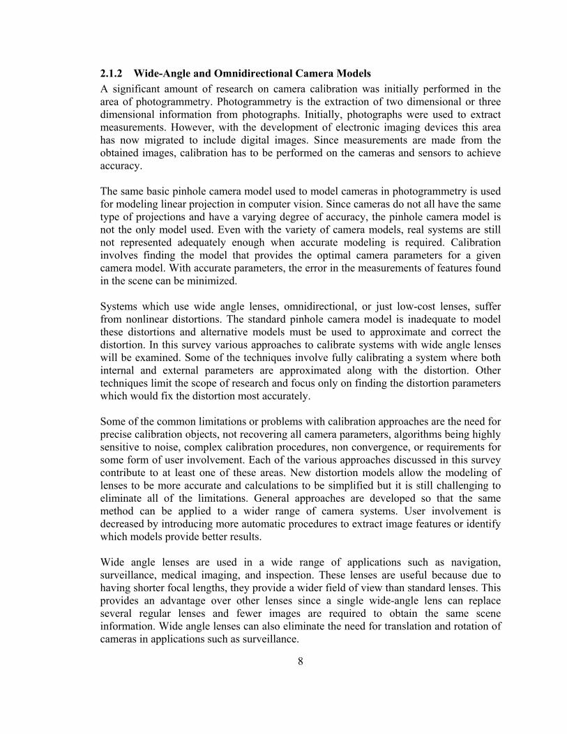
Mapping local environments with a wide-angle camera is most often seen in surveillance applications where large scenes are to be monitored. Wide angle lenses are also useful for images of an entire building from a close distance or where space is limited such as in an indoor scene. Modeling cameras with a wide field of view is challenging. The standard pinhole camera model can be used for lenses with a narrow field of view since they follow the perspective projection. When using a wide angle or fish-eye lens, a large field of view is projected onto a finite image plane. Figure 2.3 shows an example of the projection found in a fish-eye lens. Perspective projection in these cases cannot accurately model the projection of points onto the image plane. As a result, other models must be introduced to model cameras with a wide field of view. Two common approaches are widely used for modeling the way world points are projected onto the image plane in wide angle cameras. One approach is to model the projection as a deviation from the ideal pin-hole camera model [Hartley05] [Criminisi99] [Fitzgibbon01] [Thirthala05b] [Sturm05]. In this case the deviation from the perspective projection is called radial distortion. These models transform the wide field of view image to follow the pinhole model. Models for radial distortion and methods to find the radial distortion parameters will be presented in section three.

Figure 2.3: Projection of scene point onto a finite image plane found in a fish-eye lens.

10

The other common approach, which is said to be a better approach to model wide angle and fish-eye lenses, is to model the lens projection directly [Kannala04] [Broaddus05]. Just like other models, these models describe how image points are projected onto the image plane. Some lenses are manufactured to obey a particular model in which case the model information is provided by the manufacturer. Other times the type of model that a lens follows is unavailable in which case calculations must be made to determine which projection models provide better results.

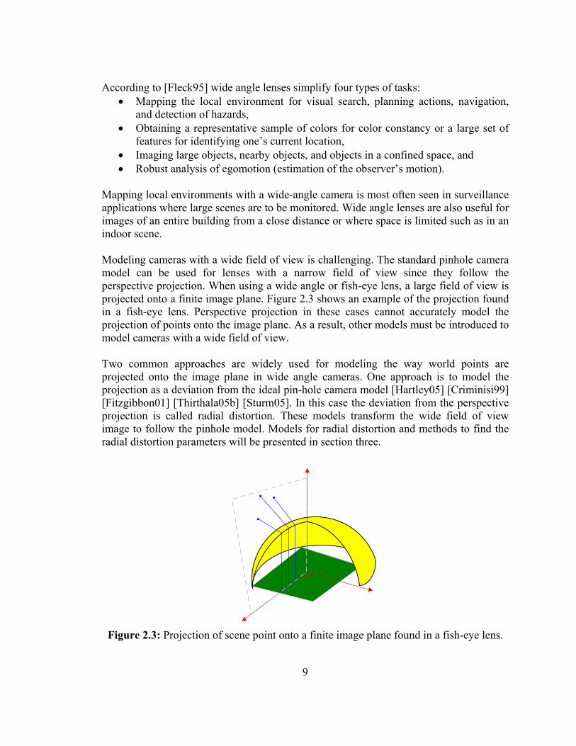
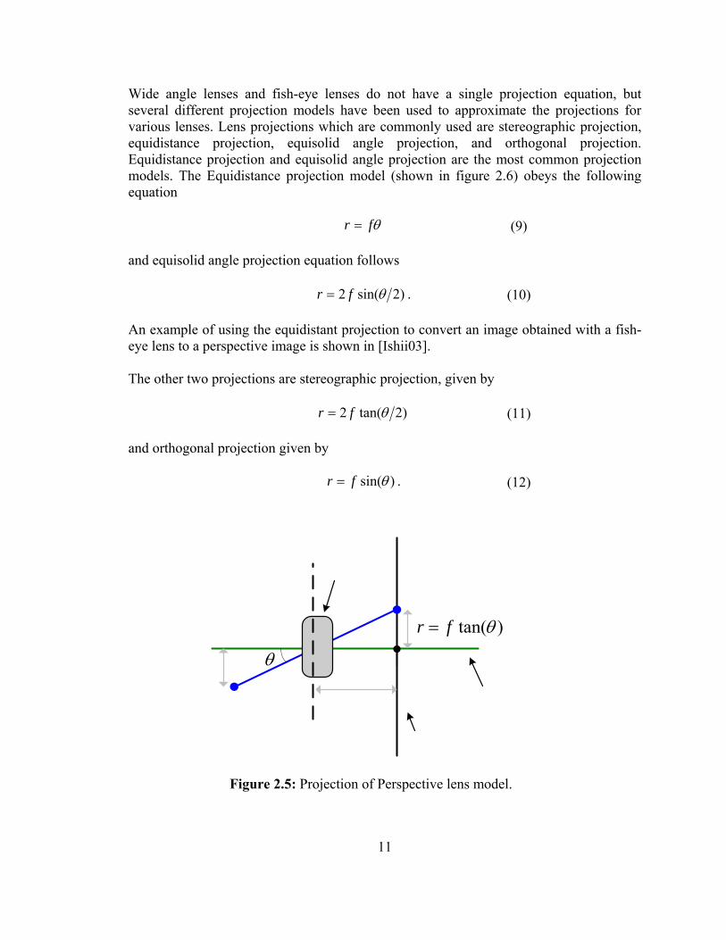
2.1.3 Lens Projections Modeling lens projections is achieved by using radially symmetric functions which map angle θ between the ray of the world point and the image plane to distance r from the image center. Figure 2.4 shows the ideal geometry of mapping point M in the scene to point m on the image plane. Perspective projection of the ideal pinhole camera (shown in figure 2.5) can be described by

)tan(θfr = (8) where r is distance between the image point and the principal point, f is the focal length, and θ is the angle between the optical axis and the point ray. In perspective projection straight lines in the world are imaged as straight lines on the image plane. As discussed earlier, wide angle lenses and fish-eye lenses can not be described by perspective projection because of the large field of view. Using perspective projection causes objects at the edges of an image to appear stretched.

M

Image planerm

f

Principle Axis

θ

Figure 2.4: Geometry of ideal lens projections.

11

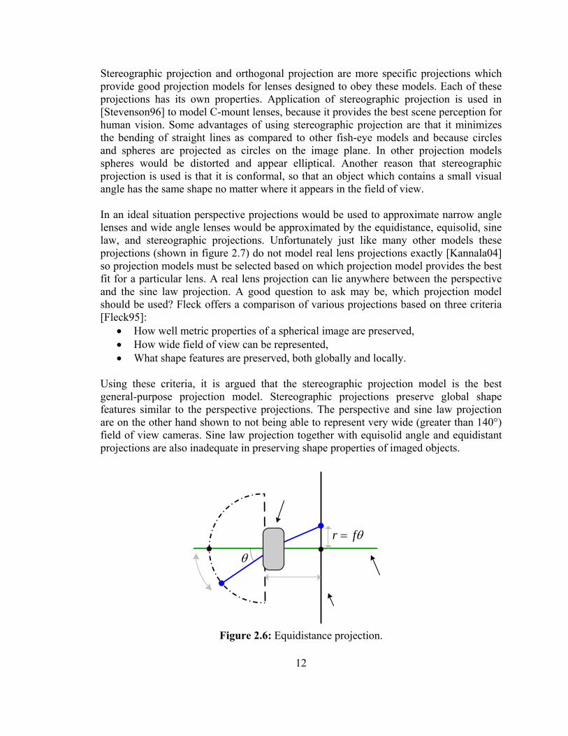
Wide angle lenses and fish-eye lenses do not have a single projection equation, but several different projection models have been used to approximate the projections for various lenses. Lens projections which are commonly used are stereographic projection, equidistance projection, equisolid angle projection, and orthogonal projection. Equidistance projection and equisolid angle projection are the most common projection models. The Equidistance projection model (shown in figure 2.6) obeys the following equation

θfr = (9) and equisolid angle projection equation follows

)2sin(2 θfr = . (10) An example of using the equidistant projection to convert an image obtained with a fish-eye lens to a perspective image is shown in [Ishii03]. The other two projections are stereographic projection, given by

)2tan(2 θfr = (11) and orthogonal projection given by

)sin(θfr = . (12)

θ

)tan(θfr =

Figure 2.5: Projection of Perspective lens model.

12

Stereographic projection and orthogonal projection are more specific projections which provide good projection models for lenses designed to obey these models. Each of these projections has its own properties. Application of stereographic projection is used in [Stevenson96] to model C-mount lenses, because it provides the best scene perception for human vision. Some advantages of using stereographic projection are that it minimizes the bending of straight lines as compared to other fish-eye models and because circles and spheres are projected as circles on the image plane. In other projection models spheres would be distorted and appear elliptical. Another reason that stereographic projection is used is that it is conformal, so that an object which contains a small visual angle has the same shape no matter where it appears in the field of view. In an ideal situation perspective projections would be used to approximate narrow angle lenses and wide angle lenses would be approximated by the equidistance, equisolid, sine law, and stereographic projections. Unfortunately just like many other models these projections (shown in figure 2.7) do not model real lens projections exactly [Kannala04] so projection models must be selected based on which projection model provides the best fit for a particular lens. A real lens projection can lie anywhere between the perspective and the sine law projection. A good question to ask may be, which projection model should be used? Fleck offers a comparison of various projections based on three criteria [Fleck95]:

• How well metric properties of a spherical image are preserved, • How wide field of view can be represented, • What shape features are preserved, both globally and locally.

Using these criteria, it is argued that the stereographic projection model is the best general-purpose projection model. Stereographic projections preserve global shape features similar to the perspective projections. The perspective and sine law projection are on the other hand shown to not being able to represent very wide (greater than 140°) field of view cameras. Sine law projection together with equisolid angle and equidistant projections are also inadequate in preserving shape properties of imaged objects.

θ

θfr =

Figure 2.6: Equidistance projection.

13

One way to find out which projection simulates a particular lens most accurately is to try all of the models and see which one produces the best results. In [Bakstein02] a cylinder with a grid wrapped around it was imaged by a wide angle camera with a 183° field of view. The projection of light rays unto the image was compared to the predicted pixel coordinates by the different projections. Stereographic projection provided the best result but there were still errors generated by using this projection model. To eliminate the error the model was extended to combine stereographic projection with equisolid angle projection into a single model represented by

⎟⎠⎞

⎜⎝⎛+⎟

⎠⎞

⎜⎝⎛=

dc

bar θθ sintan (13)

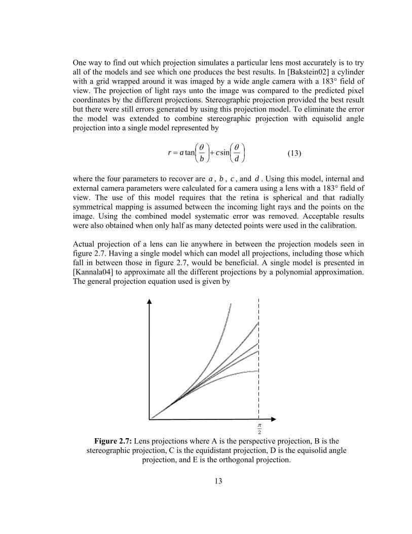
where the four parameters to recover are a , b , c , and d . Using this model, internal and external camera parameters were calculated for a camera using a lens with a 183° field of view. The use of this model requires that the retina is spherical and that radially symmetrical mapping is assumed between the incoming light rays and the points on the image. Using the combined model systematic error was removed. Acceptable results were also obtained when only half as many detected points were used in the calibration. Actual projection of a lens can lie anywhere in between the projection models seen in figure 2.7. Having a single model which can model all projections, including those which fall in between those in figure 2.7, would be beneficial. A single model is presented in [Kannala04] to approximate all the different projections by a polynomial approximation. The general projection equation used is given by

Figure 2.7: Lens projections where A is the perspective projection, B is the

stereographic projection, C is the equidistant projection, D is the equisolid angle projection, and E is the orthogonal projection.

14

...)( 7

45

33

21 ++++= θθθθθ kkkkr (14) but only the first two terms are used to model the projections. The model can be used to approximate all the projections with a moderate level of accuracy. The approximation worked well to calibrate a camera equipped with a fish-eye lens using a single image. However, to achieve more accurate results more views with a large quantity of control points should be used.

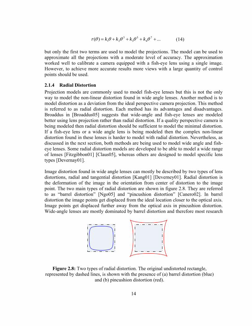
2.1.4 Radial Distortion Projection models are commonly used to model fish-eye lenses but this is not the only way to model the non-linear distortion found in wide angle lenses. Another method is to model distortion as a deviation from the ideal perspective camera projection. This method is referred to as radial distortion. Each method has its advantages and disadvantages. Broaddus in [Broaddus05] suggests that wide-angle and fish-eye lenses are modeled better using lens projection rather than radial distortion. If a quality perspective camera is being modeled then radial distortion should be sufficient to model the minimal distortion. If a fish-eye lens or a wide angle lens is being modeled then the complex non-linear distortion found in these lenses is harder to model with radial distortion. Nevertheless, as discussed in the next section, both methods are being used to model wide angle and fish-eye lenses. Some radial distortion models are developed to be able to model a wide range of lenses [Fitzgibbon01] [Claus05], whereas others are designed to model specific lens types [Devernay01]. Image distortion found in wide angle lenses can mostly be described by two types of lens distortions, radial and tangential distortion [Kang01] [Deverney01]. Radial distortion is the deformation of the image in the orientation from center of distortion to the image point. The two main types of radial distortion are shown in figure 2.8. They are referred to as “barrel distortion” [Ngo05] and “pincushion distortion” [Canero02]. In barrel distortion the image points get displaced from the ideal location closer to the optical axis. Image points get displaced further away from the optical axis in pincushion distortion. Wide-angle lenses are mostly dominated by barrel distortion and therefore most research

Figure 2.8: Two types of radial distortion. The original undistorted rectangle,

represented by dashed lines, is shown with the presence of (a) barrel distortion (blue) and (b) pincushion distortion (red).

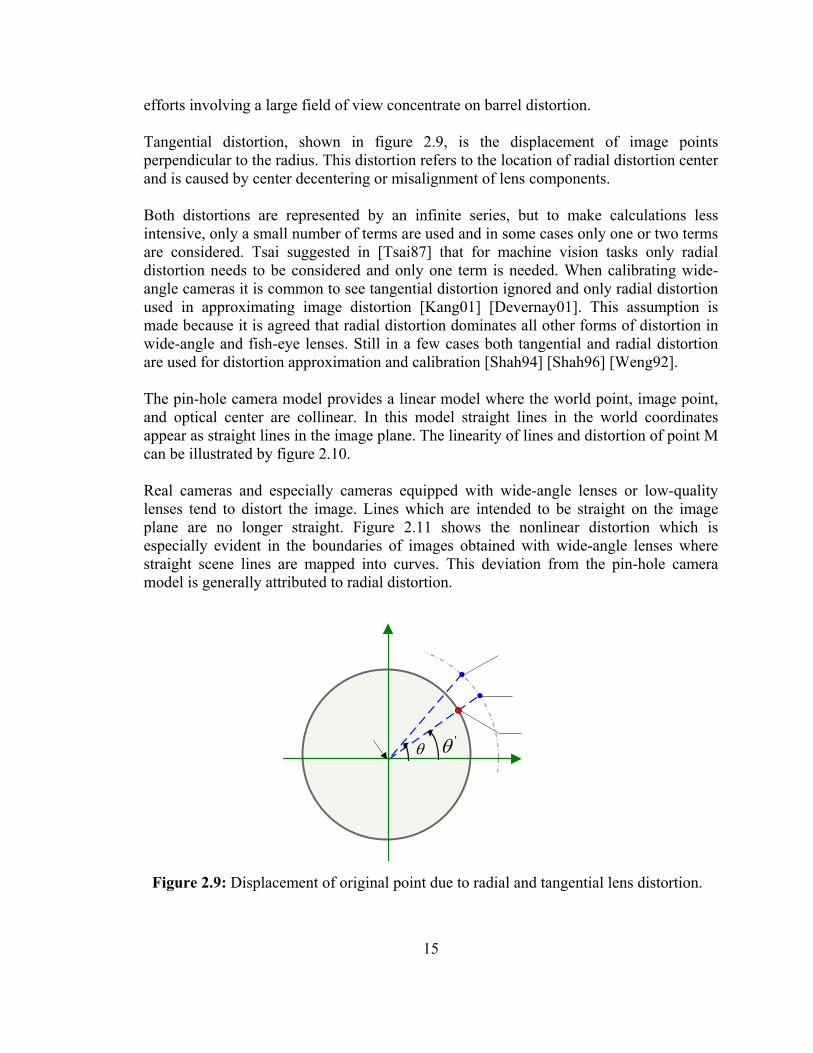
15

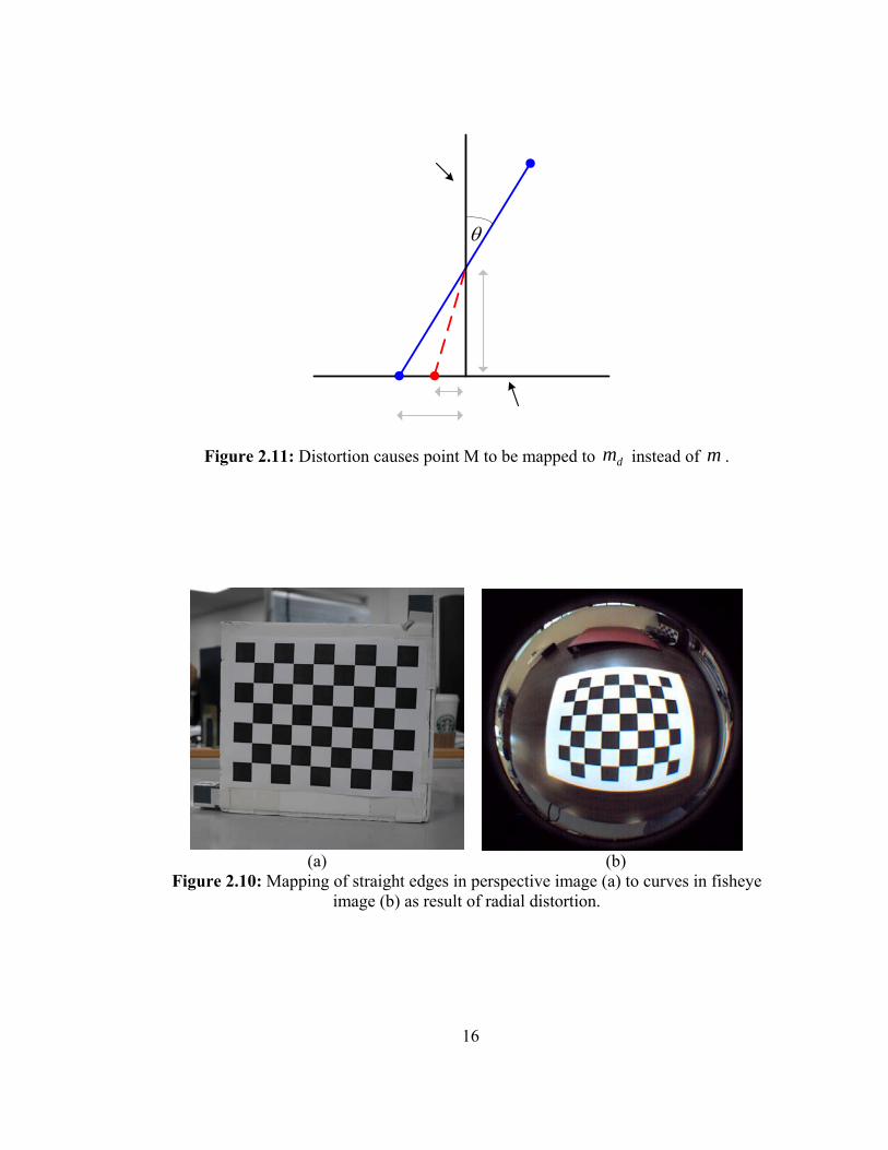
efforts involving a large field of view concentrate on barrel distortion. Tangential distortion, shown in figure 2.9, is the displacement of image points perpendicular to the radius. This distortion refers to the location of radial distortion center and is caused by center decentering or misalignment of lens components. Both distortions are represented by an infinite series, but to make calculations less intensive, only a small number of terms are used and in some cases only one or two terms are considered. Tsai suggested in [Tsai87] that for machine vision tasks only radial distortion needs to be considered and only one term is needed. When calibrating wide-angle cameras it is common to see tangential distortion ignored and only radial distortion used in approximating image distortion [Kang01] [Devernay01]. This assumption is made because it is agreed that radial distortion dominates all other forms of distortion in wide-angle and fish-eye lenses. Still in a few cases both tangential and radial distortion are used for distortion approximation and calibration [Shah94] [Shah96] [Weng92]. The pin-hole camera model provides a linear model where the world point, image point, and optical center are collinear. In this model straight lines in the world coordinates appear as straight lines in the image plane. The linearity of lines and distortion of point M can be illustrated by figure 2.10. Real cameras and especially cameras equipped with wide-angle lenses or low-quality lenses tend to distort the image. Lines which are intended to be straight on the image plane are no longer straight. Figure 2.11 shows the nonlinear distortion which is especially evident in the boundaries of images obtained with wide-angle lenses where straight scene lines are mapped into curves. This deviation from the pin-hole camera model is generally attributed to radial distortion.

θ'θ

Figure 2.9: Displacement of original point due to radial and tangential lens distortion.

16

(a) (b)

Figure 2.10: Mapping of straight edges in perspective image (a) to curves in fisheye image (b) as result of radial distortion.

θ

Figure 2.11: Distortion causes point M to be mapped to dm instead of m .

17

A number of sources provide the commonly used approximation of the relationship between a point in an image with radial distortion and an ideal non-distorted point [Hartley04] [Criminisi99]. The projection of the distorted point can be related to the ideal point by the radial lens distortion model

⎟⎟⎠

⎞⎜⎜⎝

⎛=⎟⎟

⎠

⎞⎜⎜⎝

⎛yxrL

yx

d

d )( (15)

where ),( yx is the ideal (undistorted) image position, ),( dd yx is the image position with

radial distortion, r is the radial distance 22 yx + from the center, and )(rL is the distortion factor. The radial lens distortion model can also be shown in pixel coordinates by

))(( cdc xxrLxx −+= (16)

and ))(( cdc yyrLyy −+= . (17)

where ),( dd yx are the distorted coordinates, ),( yx are the corrected coordinates, and

),( cc yx is the center of radial distortion. The radial distortion factor )(rL can be approximated by a Taylor expansion

...1)( 4

43

32

21 rkrkrkrkrL ++++= (18)

where ...),,,( 4321 kkkk are the radial correction coefficients. This model referred to as the polynomial model is the most common radial distortion model. Approximating distortion in wide-angle and fish-eye lenses requires a large number of terms. Depending on the degree of distortion, assumptions, and the approach used to correct the distortion, only a few terms are sometimes considered. In [Kang01] it is shown that recovering only 1k and

2k is sufficient for low to moderately distorted images. Shah on the other hand used a fifth and seventh order odd powered polynomial to approximate the distortion and still distortion correction was not adequate [Shah96]. In general this model works well for lenses with small amount of distortion but can become impractical to use with wide-angle or fish-eye lenses since large number of terms are required.

Another model used for approximating radial distortion of cameras is the division model [Fitzgibbon01]. The division model is similar to the polynomial model but the distortion coefficients are placed in the denominator to help approximate the true distortion. The division model is given by

18

...)1( 64

43

22 rkrkrk

xx d

+++= . (19)

Just like other distortion models, the division model assumes that the distortion center is known and that the distorted center is transformed to where the center of distortion is at the origin. This model was originally used by Fitzgibbon because it allowed him to simultaneously determine the fundamental matrix and the radial distortion between multiple views [Fitzgibbon01]. This model has advantages over the polynomial model because high distortion can be modeled with lower order or number of terms. On several occasions it has been used in calibration of wide-angle cameras [Barreto03] [Thirthala05b] [Sturm05] and in some cases only one parameter was sufficient to model the distortion [Claus05][Fitzgibbon01]. Another model that approximates radial distortion is the rational model which combines the polynomial model and the division model into a single distortion approximation [Claus05]. Claus and Fitzgibbon introduced the new rational function model to be used for wide-angle and catadioptric lenses. The rational function model provides a general and relatively simple model for modeling radial distortion generated by wide-angle lenses. This algebraic model allows the use of a linear algorithm to estimate nonlinear image distortion. Using the fact that fish-eye lenses contain some degree of nonlinear distortion a Field of View (FOV) model is developed [Devernay01]. The model provides an excellent distortion fit since the model is based on the way a fish-eye lens is designed [Claus05]. Using only one parameter, which is the field of view w , the distance between the image point and the principal point is made roughly proportional to the angle between the corresponding world point, optical center and the optical axis. The undistorted point is modeled by

⎟⎠⎞

⎜⎝⎛

=

2tan2

)tan(wwxx d .

(20)

A recent paper [Ma06] suggests a method to model radial distortion with an analytical piecewise radial distortion model. One of the goals of the calibration is to find a relationship which can easily be used to correct the distortion. In such cases it is sometimes necessary to find an inverse of the polynomial which models the distortion. Modeling nonlinear distortion with a polynomial model can cause the polynomial to become complex when modeling cheap or complex imaging systems. [Ma06] suggest to break up the standard polynomial model into several segments. This method provides an easier method to find the inverse of each section and easily perform the undistortion of the images. Other models have been developed to approximate radial distortion for not only wide-angle and fish-eye lenses, but also for other non-standard cameras with curved mirrors [Barreto04] [Ying04] [Hartley97].

19

Tangential distortion was presented by Conrady in [Conrady19] back in 1919. As discussed in the preceding sections tangential distortion is generally due to imperfections found in multi-element lenses. The effect is seen by the shift of image point along and tangential to the radial direction from the principal point. As seen in figure 2.9. All imaging systems have some degree of tangential distortion [Swaminathan01]. Tangential distortion is not noticeable in images and is often assumed to be insignificant in the distortion models for wide-angle and fish-eye lenses. Due to substantial presence of radial distortion, tangential distortion is considered to be a minor source of distortion. In [Mallon04] while working with radial image distortion, tangential distortion is ignored because of its unclear presence and since only small levels of it could be reduced. Another reason for not including it in the calculations is that without it the distortion model is simplified.

2.2 General Calibration General calibration methods can be divided into three major categories. The first group of methods uses calibration objects with feature points whose world 2D or 3D coordinates are accurately known. The calibration objects and feature points can be found in a wide range of shapes and forms. The more commonly used calibration objects are planar checkerboards but patterns with circles, squares, and dots are also used. This method is sometimes referred to as test-range calibration, where pre-determined features with known 2D or 3D coordinates are used as the calibration reference. The second category of calibration methods does not rely on known feature points coordinates but uses the geometric invariants of image features. This group of nonmetric methods uses features such as straight lines or spheres to perform the calibration. Other approaches use point correspondence between multiple images to obtain the calibration parameters. The third category, self-calibration sometimes referred to as weak- calibration, does not use any known calibration objects. Camera parameters are estimated from a sequence of images by using camera intrinsic constraints, motion constraints, or scene constraints. In most cases the internal camera parameters are kept fixed while multiple images are obtained of a scene. The correspondence of the images is then used to estimate internal and external parameters. This method has also been extended to varying internal parameters caused by changing the zoom or focus but other constraints or assumptions have to be introduced.

2.2.1 Test-Range Calibration With Test-Range calibration it is necessary to have a controlled object space. The controlled object space consists of manufactured calibration patterns or objects whose 2D or 3D coordinates are known with good precision. Known coordinates of the calibration object are used together with the extracted coordinates from a sequence of images to approximate the calibration parameters.

20

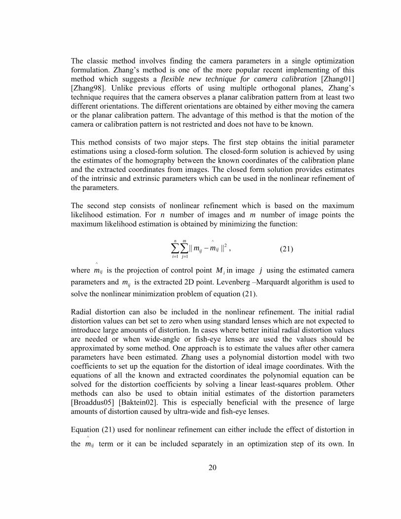
The classic method involves finding the camera parameters in a single optimization formulation. Zhang’s method is one of the more popular recent implementing of this method which suggests a flexible new technique for camera calibration [Zhang01] [Zhang98]. Unlike previous efforts of using multiple orthogonal planes, Zhang’s technique requires that the camera observes a planar calibration pattern from at least two different orientations. The different orientations are obtained by either moving the camera or the planar calibration pattern. The advantage of this method is that the motion of the camera or calibration pattern is not restricted and does not have to be known. This method consists of two major steps. The first step obtains the initial parameter estimations using a closed-form solution. The closed-form solution is achieved by using the estimates of the homography between the known coordinates of the calibration plane and the extracted coordinates from images. The closed form solution provides estimates of the intrinsic and extrinsic parameters which can be used in the nonlinear refinement of the parameters. The second step consists of nonlinear refinement which is based on the maximum likelihood estimation. For n number of images and m number of image points the maximum likelihood estimation is obtained by minimizing the function:

∑∑= =

−n

i

m

jijij mm

1

2

1

^|||| , (21)

where ijm^

is the projection of control point iM in image j using the estimated camera parameters and ijm is the extracted 2D point. Levenberg –Marquardt algorithm is used to solve the nonlinear minimization problem of equation (21). Radial distortion can also be included in the nonlinear refinement. The initial radial distortion values can bet set to zero when using standard lenses which are not expected to introduce large amounts of distortion. In cases where better initial radial distortion values are needed or when wide-angle or fish-eye lenses are used the values should be approximated by some method. One approach is to estimate the values after other camera parameters have been estimated. Zhang uses a polynomial distortion model with two coefficients to set up the equation for the distortion of ideal image coordinates. With the equations of all the known and extracted coordinates the polynomial equation can be solved for the distortion coefficients by solving a linear least-squares problem. Other methods can also be used to obtain initial estimates of the distortion parameters [Broaddus05] [Baktein02]. This is especially beneficial with the presence of large amounts of distortion caused by ultra-wide and fish-eye lenses. Equation (21) used for nonlinear refinement can either include the effect of distortion in

the ijm^

term or it can be included separately in an optimization step of its own. In

21

[Zhang98] the radial distortion parameters are refined together in a single nonlinear optimization estimation since splitting up the procedure into two separate alternated refinement steps showed that the convergence was slow. In [Broaddus05] on the other hand the process was split up into what is called bundle adjustment because it showed improvements when certain lens projections were used. In bundle adjustment first the initial estimates of camera parameters are refined using a nonlinear optimization method without including the distortion parameters. For a survey of theory and methods of bundle adjustment used in photogrammetry and computer vision refer to [Triggs00]. Then the refinement is repeated by minimizing the function using just the distortion parameters. Both radial distortion and tangential distortion are included in the nonlinear refinement. Splitting up the nonlinear optimization showed that bundle adjustment method provides significantly better results compared to performing the refinement of all the parameters simultaneously as the projection model deviates from the standard perspective projection [Broaddus05]. Perspective and orthogonal projections showed none or little benefit in alternating the refinement but stereographic and equisolid projections showed significant estimation improvement when bundle adjustment was implemented. Bundle adjustment to perform nonlinear optimization can provide better performance if wide-angle or fish-eye lenses are used. An approach to accurately calibrate a wide-angle or fish-eye lens in a single optimization step is to use special conditions and lens projections. When working with lenses that introduce large amounts of distortion it is sometimes beneficial to use special projections to find the initial estimates of distortion parameters to be used in the nonlinear refinement. In [Bakstein02a] and [Bakstein02b] a fish-eye lens with a field-of-view greater than 180° is calibrated by using a known 3D calibration object and implementing the Levenberg –Marquardt algorithm to refine all the camera parameters simultaneously. Distortion was approximated by using commonly used projection models discussed in the previous section. The best results were generated by using the stereographic projection but since there were still errors the model was extended to also include equisolid angle projection. This model generated four parameters which are estimated together with other camera model parameters in the nonlinear refinement. An assumption made in this implementation is that the skewness of the image axes is negligible since most cameras have orthogonal pixels. Combining the complete camera model results in 13 parameters to be refined. The initial values of the image center are set to the center of the circle resulting from the outside perimeter of the fish-eye lens. Parameters of the lens projection were initially set to ideal stereographic projection. The ratio representing the difference in scale of horizontal and vertical axis is set to 1. All of the parameters were initialized and then refined using the Levenberg –Marquardt algorithm. A single image of a calibration pattern is used to provide the relationship between the light rays and pixels in the image. It has been suggested that non-linear optimization methods require good initial values. If the initial values are not good enough the non-linear optimization will not converge or inaccurate results will be generated. Another problem suggested by numerous researchers

22

is that some of these methods do not eliminate the coupling between internal parameters which include distortion parameters and external parameters. Calibration method presented in [Zhang01] considers an even-order polynomial model with only the first few distortion coefficients. This commonly used radial distortion model does not always provide accurate results for systems with wide field-of-view. Many other distortion models and lens projections can be used to estimate the distortion. Parameter free distortion calibration methods are being developed to get away from being restricted to the type of lens which can be calibrated with a specific distortion model. In [Hartley05] a method is presented to estimate radial distortion of the camera simultaneously with other camera parameters. This method does not assume any specific distortion model but finds a curve which relates the distortion of a point to the distance it is away from the center of distortion. The first requirement is to determine the center of distortion in the image. Unlike other methods which assume that the center of distortion is in the center of the image or at the principal point, Hartley and Kang present a simple method to estimate the center of distortion which turns out to be significantly different from the image center and the principal point. To find the center of distortion a planar calibration pattern with known coordinates is compared to the extracted coordinates from a distorted image. Since with radial distortion ideal points expand outward from the distortion center the epipole of the image extracted from the fundamental matrix is the distortion center. Tangential distortion is ignored and only radial distortion is considered. The next step is to find the homographies which map the calibration grid to the image plane. To simplify the calculations the coordinates are changed so that the origin is at the previously calculated image center. With the change in the coordinates the first two rows of the homography matrix can be directly extracted from the fundamental matrix but the third row is still arbitrary. Several different methods exist to determine the last row of the homography matrix but since a parameter-free method is preferred two assumptions must be made. The first assumption is that the distortion is circularly symmetric about the center of distortion. This assumption should hold if the pixels are square but as the authors have shown it is not critical for the success of this method. The second assumption is that with distortion the radial distance of points from the center of distortion is a monotonic function of the distance without distortion. This condition naturally holds for any real camera system since every point in the scene does not appear more than once on the image. With these assumptions if the last row of the homography matrix is estimated correctly then the curve relating distorted and corrected points will be monotonic and contain small amounts of noise. If on the other hand the last row is incorrectly estimated the result would be an irregularly scattered plot. The goal becomes to find the values for the last row of the homography matrix which produces the smoothest monotonic curve. One way to accomplish this is a simple least squares technique. With careful manipulation of the total squared variance equation of adjacent points on the distortion curve the problem is simplified into a linear least square problem. The results were

23

refined with a non-linear minimization but the improvements obtained were minimal. Another approach to find the last row of the homography matrix using the monotonicity constraint is to use the local linearity assumption. In this method it is assumed that the points in the radial distortion curve are locally linear. This can easily be used if a large number of samples are available for the distortion curve. With a good monotonic distortion curve any commonly available method can be used to approximate the curve. With the homography matrix of each image approximated any method can be used to find the calibration parameters. The method can easily be used together with other calibration approaches such as the one presented by [Zhang01]. Hartley and Kang method offers an advantage over other methods because it presents a technique to estimate the radial distortion function and homographies in a parameter-free approach. This allows the approach to work with many different lenses and camera systems without being limited to any particular distortion or projection model. Another advantage of this approach is that it uses linear approximations but non-linear methods can be implemented at many stages of the process. Ignoring the sensitivity to noise this method can also be adapted to work without a calibration pattern or with an auto-calibration technique. Even though the results of this method do not provide high accuracy it offers the advantage of a fast non-iterative method which can be used with other common calibration techniques.

2.2.2 Non-metric Calibration Unlike test-range calibration methods, non-metric calibration methods do not require a controlled object space whose measurements are accurately known in the 3D world. These methods use invariants of image features such as straight lines [Devernay01], parallel lines with vanishing point constraints, or images of spheres [Agrawal03] and [Zhang05]. Other methods use point correspondence from multiple views to locate the image features. The advantage of these methods is that some can perform image distortion correction without prior camera calibration. This is beneficial when the original equipment used to capture the scene is not available such as in archived footage. In these situations the calibration is achieved by first observing the archived footage and picking out scenes which contain the necessary features for calibration. Most nonmetric camera calibration methods focus on calibrating wide-angle lens distortion. These methods use the knowledge of how image features with distortion will behave and how these features should appear without distortion. The most widely used approach is to use the fact that straight lines should be straight in an undistorted image. Nonlinear distortion caused straight lines to appear curved. Distortion is minimized by finding distortion parameters which make the curved lines straight. Point correspondence has been widely used in many portions of calibrating both standard cameras and cameras that introduce large amounts of distortion. Correspondence has also been used in all calibration methods including test-range calibration, non-metric calibration, and self-calibration. In test-range calibration methods the known coordinates

24

of a calibration pattern are used. Point correspondence is most often used to estimate the fundamental matrix from point correspondence of two images. Different numerical methods [Hartley03] exist for estimating the fundamental matrix from point correspondence. Images of spheres are also used to extract calibration parameters. An advantage of using a sphere as a calibration object is that it is an object of revolution which can be observed by multiple cameras simultaneously. Planar patterns can be observed with multiple cameras only if the camera’s field-of-view is in front of the pattern but with an object of revolution the cameras can be positioned from any angle with respect to the object. Both nonlinear [Agrawal03] and linear [Zhang05] procedures have been used to calculate the camera parameters. These methods require the extraction of apparent contours from either three images of a sphere or a single image of three spheres. In [Agrawal03] the dual image of an absolute quadric is used together with semi-definite programming to find an exact solution without initialization but involving nonlinear operations. In [Zhang05] on the other hand a linear approach is used which can provide faster calibration. Both of the mentioned methods do not include the estimation of distortion but [Agrawal03] plan to look into the effects of lens distortion on the calibration.

2.2.3 Self-Calibration In self-calibration camera parameters are estimated which are consistent with predetermined constraints based on projective geometry. The more commonly used constraints are camera intrinsic constraints, camera motion constraints, and scene constraints. A review of recent advances on camera self-calibration can be found in [Hemayed03]. Most of the research in self-calibration concentrates on standard cameras which do not have extreme image distortions and as a result radial and tangential distortions are often ignored or assumed to be insignificant. In the context of this thesis, we will only consider calibration methods which include lens distortion. Self-calibration methods using pure rotation have been shown to be sensitive to radial distortion [Tordoff04] [Tordoff00]. Both pin-cushion distortion and barrel distortion will cause inaccurate calibration results. It is also shown that estimating even a single distortion coefficient is difficult during self calibration. To obtain self-calibration from pure rotation it is required that all rays pass through the rotation center and 3D lines joining corresponding points should meet at the rotation center. Figure 2.12 is an illustration from Tordoff and Murray’s work [Tordoff04] showing that the conditions are met with no distortion present but the calibration fails if the lens exhibits distortion. With distortion the image points are displaced and the 3D lines joining the corresponding points are no longer meeting at the rotation center.

25

From the displacement of the line intersection, the presence of pin-cushion distortion causes an under-estimate of the lens’ focal length and barrel distortion causes an over-estimate. If barrel distortion is increased substantially self-calibration will fail. This theory based on geometrical optics was also shown to be consistent with experiments performed on real data. Results with synthetic simulation showed that with pin-cushion distortion the self-calibration algorithm is tolerant but is highly sensitive to barrel distortion. The experiment also showed that under barrel distortion at a fixed focal length of 2000 pixels the calibration was unreliable at distortion coefficient value of

8106 −×−≈k and was completely unstable at values around 8108 −×−≈k . The authors also derive the equation which is consistent with the experiments to estimate the distortion coefficient value at which breakdown of the method will occur. The equation is given by

231f

kb −≈ , (22)

where bk is the distortion coefficient value and f is the focal length. Tordoff and Murray also present four different approaches to fix distortion [Tordoff04]. The first approach is to correct distortion by pre-calibrating the distortion. The pre-calibration of a system will provide a cost function which relates the distortion and the focal length for the particular system. The other methods do not use any a priori information. One method uses bundle adjustment to minimize the error but with this method good initial values must be supplied. Another method uses the assumption that the distortion is modeled by a function over a number of consecutive frames. The fourth method presented uses a known distortion model to minimize the error in an iterative manner. Since even small amounts of distortion can have a significant effect on self-calibration methods, the distortion has to be corrected before they can be implemented. Research done by Meng and Zhuang specifically focuses on calibrating lens distortion [Meng04]. A self-calibration method is achieved by using point correspondence from two images.

Figure 2.12: Effect of radial distortion on 3D lines joining sets of corresponding points for (a) no distortion, (b) pin-cushion distortion, and (c) radial distortion [Tordoff04].

26

Epipolar transformation is used to measure and minimize the epipolar distance and estimate the optimal camera parameters. More on this approach will be discussed in the next section on distortion calibration. Attempts have been made to include nonlinear lens distortion with the estimation of the fundamental matrix from point correspondence found in two views [Fitzgibbon01] [Micusik03]. This approach would provide contributions to the problems of self-calibration and structure from motion found in systems with the presence of radial lens distortion. Fitzgibbon presents a linear approach to simultaneously estimate the fundamental matrix and one radial distortion term. This is achieved by abandoning the standard polynomial distortion model and adopting the division model for distortion. The division model provides another equation for approximating the actual distortion curve. Fitzgibbon showed that the division model is just as accurate as the traditional polynomial model. With this distortion model it is possible to incorporate one distortion term into a linear estimation of the fundamental matrix by using the 8-point algorithm. The estimation of the fundamental matrix with one distortion term from the division model allows the estimation to become a quadratic eigenvalue problem for which numerical algorithms are readily available. The implementation of this approach on real and synthetic data showed that in some cases the approach provides stable results. One limitation found from synthetic data which is also found in other approaches is that this method works well in the presence of large amounts of distortion. If only a small amount of distortion is present then the technique will not provide accurate estimations of the distortion parameter. On the other hand, the implementation of this method on real data with RANSAC showed that more point correspondences are found even for small amounts of distortion. This method has also been expanded by Micusik and Pajdla [Micusik03] to work with omnidirectional systems since Fitzgibbons method can not be used for camera systems with a view angle of more than 180º. The model used for the omnidirectional camera has multiple parameters but in order to have a solvable quadratic eigenvalue problem the model needs to be simplified. The two assumptions which allow the simplification are that the view field is circular on the sensor plane and that the view angle is approximately known. The simplified model is then linearized so that the quadratic eigenvalue problem can be formulated. With these assumptions the approach used by [Fitzgibbon01] is implemented with an omnidirectional lens. Most of the research on self-calibration methods focuses on active vision systems since the calibration can be done without calibration patterns and with limited constraints. Self-calibration has not been widely applied to omnidirectional systems since even small amounts of distortion can cause instability. If systems are used which exhibit lens distortion, then distortion must be fixed before useful results can be obtained.

27

2.3 Wide-Angle Distortion Calibration To obtain better initial parameters for the optimization step and reduce the influence of coupling between intrinsic and extrinsic parameters recent efforts have been made to find good distortion parameter approximations before proceeding to full camera calibration. Traditional methods of camera calibration include the calibration of distortion parameters together with the calibration of intrinsic and extrinsic parameters. Distortion parameters in these methods are initially roughly estimated or just set to zero. Providing incorrect initial estimates of these parameters can cause the results to be unstable and convergence not to occur. The nonlinear optimization step also needs some type of criteria to know when an adequate solution has been obtained. Due to the significant amount of lens distortion in cameras with medium and wide angle lenses the traditional calibration methods can only provide less accurate results and/or result in longer non-linear optimization time [El-Melegy03]. There is also some kind of coupling between camera internal, external, and distortion parameters [El-Melegy03] [Weng92]. To achieve more stable and accurate results, methods have been proposed which approximate lens distortion parameters separate from the calibration of camera parameters. The traditional approach involves solving for distortion parameters in the last part of the calibration process, where the parameters are minimized in a nonlinear optimization algorithm [Zhang98]. Lens distortion parameters and other intrinsic and extrinsic camera parameters are estimated simultaneously in a single optimization step. An analytical approach to solving for radial distortion parameters before the optimization step can provide smaller error in the calibration parameters [Graf05]. The closed form approach alters the classical calibration algorithm by removing the determination of the radial distortion parameters from the final optimization algorithm. Radial distortion parameters are determined analytically from the projection matrix and the transformation of the calibration plane. The classical error function is used while all of the other parameters are kept fixed. With the distortion parameters completely determined the proposed technique allows a reduced search space (11 parameters) in the nonlinear optimization algorithm. An advantage of this method is that the estimations of the distortion parameters are now correct and better starting values are available for the nonlinear optimization algorithm. The approach showed smaller error values in the calibration error function or smaller number of iterations required in the optimization algorithm using a wide range of cameras. Calibration approaches which simultaneously calculate the radial distortion function and camera internal parameters together are also being developed [Hartley05] [Fitzgibbon01]. For example in [Hartley05] a non-iterative approach is presented which solves for radial distortion in a parameter-free method. As a result a variety of distortion models for narrow angle and wide angle lenses can be implemented. In [Fitzgibbon01] point correspondence is used to simultaneously estimate one radial distortion parameter and the fundamental matrix.

28

Since distortion in wide angle lenses is so significant and traditional methods cause complications in the calibration process, some calibration techniques separate the estimation of the distortion parameters and other internal and external camera parameters. Other methods still include the approximation of the distortion parameters together with other camera parameters. Calibration methods involving radial distortion can be broken up into two major groups: line based calibration and point correspondence based calibration.

2.3.1 Line Based Calibration In the line based calibration approach the notion that the projection of every 3D line in a scene should appear as a line in the 2D image plane is used. One of the early works in this area was performed by Brown who used multiple parallel plumb lines to compute radial distortion using iterative gradient descent technique [Brown71]. This method uses one-dimensional lines in images to approximate distortion parameters where only distortion calibration is considered. In most approaches using this technique distortion parameters are approximated by finding which parameter values produce the straightest lines. How severe the distortion is in an image is observed by measuring the degree of distortion in the lines which are intended to be straight. Once the distortion parameters have been approximated and image distortion corrected other standard techniques can be used to extract camera internal and external parameters. In most cases distortion is calibrated without knowing anything about internal camera parameters. With this method any camera can be considered as a pinhole camera once the distortion function has been used to correct the distorted image. Unlike other methods which require multiple images, line based calibration can work well using a single image as well as multiple images [Cucchiara03] [Kang01] [Brauer-Burchard01] [Devernay01] [Geyer02]. Difficulty with this approach is that the scene must contain strong contrast straight lines and in most cases knowledge of where the lines are located must be available. Lines in the image which represent lines from the scene must be selected manually by picking points which correspond to points located on the line. The addition of more points provides data redundancy which helps when using images with noise and/or error coming sting from the point selection procedure. In some cases algorithms are developed to find edges in an image which represent lines but some form of user involvement is till required [Kang01]. A disadvantage of this method is not having the ability to automatically extract the distorted lines without errors. With distortion straight lines form curves on the distorted image plane and it becomes more difficult to automatically discriminate between which edges represents lines and which actually represent curved features in an image. The advantages of the line based method are that it is simple, fast, and more robust than other alternatives such as point matching approaches. An advantage of extracting and using lines which are already in an image is that no extra calibration points or objects are required. The distortion can be estimated and corrected from the features already present in the images.

29

2.3.1.1 Extracting Lines and Edges In some approaches distorted lines are extracted from the image manually [Swaminathan01]. The user selects points in the image along the distorted curves which represent straight lines. Then these points are used to approximate the distortion in the image. With the distortion approximated a corrected image can be generated from which other camera calibration parameters are extracted. A semi-automatic extraction of lines is presented in [Kang01]. The user manually draws lines on the image which contains projections of straight 3-D lines in the scene. Then snakes which represent deformable contours are used to search for the best-fitting lines. The process is semi-automatic because both user involvement and an algorithm are used to find the exact location of the line. First the user draws where the distorted lines are located. The lines drawn do not have to be exact because they only provide the starting values for the algorithm to find the exact location of the lines. This approach works especially well for images with substantial amounts of noise. A problem with this method is that with bad initial placement of the lines the method may not be stable. In order to have a more automatic method to extract distorted lines, outliers have to be eliminated from the lines being used for the calculations. Two papers present methods which try to reduce the effects of outliers on distortion calibration [Devernay01] [Ahmed05]. Incorrect data caused by outliers can be generated by two major factors. One is that the image may contain curves which might be mistaken as projections of straight lines. The other possible source of outliers is caused by the linking of several edges which should be separate lines. This can be shown in figure 2.13 where different edges of the picture frame are linked together and as a result are considered to be a single distorted line. Some outliers in [Devernay01] are removed by repeating the distortion minimization and polygonal approximation. Sub-pixel edge detection is fist performed on the distorted image. Then polygonal approximation is done using very small tolerances. Distortion parameters are found by measuring how much each detected segment is distorted. By repeating the distortion minimization and polygonal approximation some outliers are eliminated and more useful line segments are generated for the next iteration. Even though some outliers can be eliminated this method would not work well if severe distortion is present, when many line segments are broken up into smaller edges, or when too many outliers are present in the data [Ahmed05]. Ahmed and Farag use the least-median-of-squares to estimate the distortion parameters and help to eliminate outliers [Ahmed05]. Sub-pixel edge detection and polygonal approximation are also performed in this method. Unlike [Davernay01] large tolerances for the polygonal approximation are used. This results in longer edge chains with the possibility of joining different edge segments but since the least-median-of squares method is used to approximate the distortion parameters some of the incorrect data is eliminated in the process. This is possible because the least-median-of-squares method is very robust to false data caused by outliers. Using this method the authors claim that

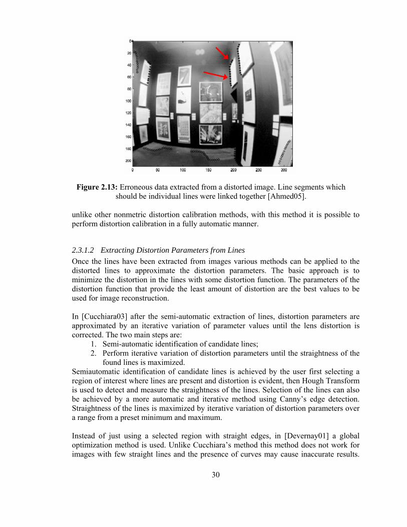
30

unlike other nonmetric distortion calibration methods, with this method it is possible to perform distortion calibration in a fully automatic manner.

2.3.1.2 Extracting Distortion Parameters from Lines Once the lines have been extracted from images various methods can be applied to the distorted lines to approximate the distortion parameters. The basic approach is to minimize the distortion in the lines with some distortion function. The parameters of the distortion function that provide the least amount of distortion are the best values to be used for image reconstruction. In [Cucchiara03] after the semi-automatic extraction of lines, distortion parameters are approximated by an iterative variation of parameter values until the lens distortion is corrected. The two main steps are:

1. Semi-automatic identification of candidate lines; 2. Perform iterative variation of distortion parameters until the straightness of the

found lines is maximized. Semiautomatic identification of candidate lines is achieved by the user first selecting a region of interest where lines are present and distortion is evident, then Hough Transform is used to detect and measure the straightness of the lines. Selection of the lines can also be achieved by a more automatic and iterative method using Canny’s edge detection. Straightness of the lines is maximized by iterative variation of distortion parameters over a range from a preset minimum and maximum. Instead of just using a selected region with straight edges, in [Devernay01] a global optimization method is used. Unlike Cucchiara’s method this method does not work for images with few straight lines and the presence of curves may cause inaccurate results.

Figure 2.13: Erroneous data extracted from a distorted image. Line segments which should be individual lines were linked together [Ahmed05].

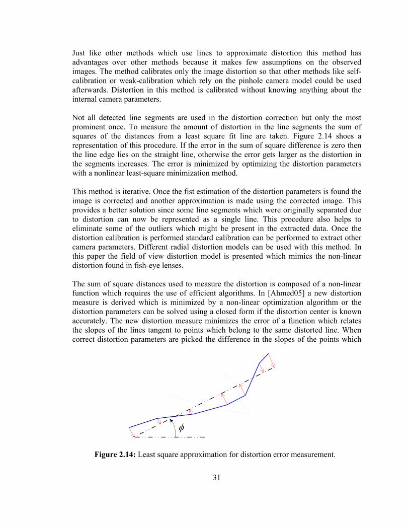
31

Just like other methods which use lines to approximate distortion this method has advantages over other methods because it makes few assumptions on the observed images. The method calibrates only the image distortion so that other methods like self-calibration or weak-calibration which rely on the pinhole camera model could be used afterwards. Distortion in this method is calibrated without knowing anything about the internal camera parameters. Not all detected line segments are used in the distortion correction but only the most prominent once. To measure the amount of distortion in the line segments the sum of squares of the distances from a least square fit line are taken. Figure 2.14 shoes a representation of this procedure. If the error in the sum of square difference is zero then the line edge lies on the straight line, otherwise the error gets larger as the distortion in the segments increases. The error is minimized by optimizing the distortion parameters with a nonlinear least-square minimization method. This method is iterative. Once the fist estimation of the distortion parameters is found the image is corrected and another approximation is made using the corrected image. This provides a better solution since some line segments which were originally separated due to distortion can now be represented as a single line. This procedure also helps to eliminate some of the outliers which might be present in the extracted data. Once the distortion calibration is performed standard calibration can be performed to extract other camera parameters. Different radial distortion models can be used with this method. In this paper the field of view distortion model is presented which mimics the non-linear distortion found in fish-eye lenses. The sum of square distances used to measure the distortion is composed of a non-linear function which requires the use of efficient algorithms. In [Ahmed05] a new distortion measure is derived which is minimized by a non-linear optimization algorithm or the distortion parameters can be solved using a closed form if the distortion center is known accurately. The new distortion measure minimizes the error of a function which relates the slopes of the lines tangent to points which belong to the same distorted line. When correct distortion parameters are picked the difference in the slopes of the points which

φ

Figure 2.14: Least square approximation for distortion error measurement.

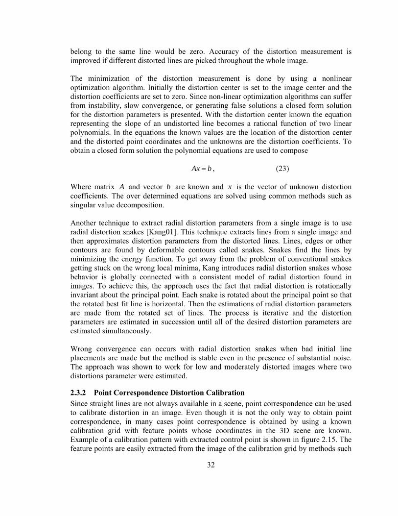
32

belong to the same line would be zero. Accuracy of the distortion measurement is improved if different distorted lines are picked throughout the whole image.

The minimization of the distortion measurement is done by using a nonlinear optimization algorithm. Initially the distortion center is set to the image center and the distortion coefficients are set to zero. Since non-linear optimization algorithms can suffer from instability, slow convergence, or generating false solutions a closed form solution for the distortion parameters is presented. With the distortion center known the equation representing the slope of an undistorted line becomes a rational function of two linear polynomials. In the equations the known values are the location of the distortion center and the distorted point coordinates and the unknowns are the distortion coefficients. To obtain a closed form solution the polynomial equations are used to compose

Ax b= , (23)

Where matrix A and vector b are known and x is the vector of unknown distortion coefficients. The over determined equations are solved using common methods such as singular value decomposition. Another technique to extract radial distortion parameters from a single image is to use radial distortion snakes [Kang01]. This technique extracts lines from a single image and then approximates distortion parameters from the distorted lines. Lines, edges or other contours are found by deformable contours called snakes. Snakes find the lines by minimizing the energy function. To get away from the problem of conventional snakes getting stuck on the wrong local minima, Kang introduces radial distortion snakes whose behavior is globally connected with a consistent model of radial distortion found in images. To achieve this, the approach uses the fact that radial distortion is rotationally invariant about the principal point. Each snake is rotated about the principal point so that the rotated best fit line is horizontal. Then the estimations of radial distortion parameters are made from the rotated set of lines. The process is iterative and the distortion parameters are estimated in succession until all of the desired distortion parameters are estimated simultaneously. Wrong convergence can occurs with radial distortion snakes when bad initial line placements are made but the method is stable even in the presence of substantial noise. The approach was shown to work for low and moderately distorted images where two distortions parameter were estimated.

2.3.2 Point Correspondence Distortion Calibration Since straight lines are not always available in a scene, point correspondence can be used to calibrate distortion in an image. Even though it is not the only way to obtain point correspondence, in many cases point correspondence is obtained by using a known calibration grid with feature points whose coordinates in the 3D scene are known. Example of a calibration pattern with extracted control point is shown in figure 2.15. The feature points are easily extracted from the image of the calibration grid by methods such

33

as Harris corner detection. Using known 3D coordinates of the calibration grid and the extracted 2D coordinates from the image, calculation can be performed by using homography matrices of the obtained images. Homography is simply the linear projective estimation defined by

ii HXx = (24) where H defines the projection of scene point iX onto the image point ix . Given four or more points correspondences the homography matrix can be estimated by a linear method [Hartely05a]. Using more than four points the least square solution can be obtained from the over-determined system. Without the presence of noise and lens distortion exact solutions can be obtained for the homography matrix, otherwise approximated solutions are obtained. Using the homography matrix from a series of images, estimations are made of the distortion, intrinsic, and extrinsic parameters. This is a very common method in the calibration of standard cameras which are modeled using the standard pinhole camera model. When wide-angle lenses are used distortion also has to be taken into account. In some methods using point correspondence the approximation of the distortion parameters is completely separated from finding the intrinsic and extrinsic camera parameters. In [Kannala04] on the other hand calibration is performed by separating the calculation of distortion and intrinsic parameters from the extrinsic parameters calculations. First intrinsic and distortion parameters are calculated by an iterative minimization then another optimization step is performed except now with the extrinsic parameters included in the minimization. First initial guesses are made for values of internal camera parameters which include the distortion parameters. The distortion parameters are fitted to one of the lens projections, the focal length is set to the manufactures specifications, and the principal point is extracted from the image. Next, to refine the initial internal parameters and find the

Figure 2.15: Sample calibration pattern with extracted control points.

34

homography matrix for each image an iterative search is performed. In the iterative search, the extracted points are projected onto the center of the image and the planer homography is found for each image between the calibration pattern coordinates and projected points. With the internal parameters refined and the error minimized, external parameters are initialized. Using the internal and external parameters the projection matrix, which relates how control points are projected in each image, is computed. The final step is the refinement of camera parameters by minimizing the sum of squared distances between the measured and modeled control point projections by using algorithms such as the Levenberg-Marquardt. To achieve a more accurate calibration, Kannala and Brandt modified their method to work with circular control points [Kannala04]. The control point coordinates can be obtained with sub-pixel accuracy by finding the centroids of white circles located on a black background. With this method a single view is used to calibrate a camera when calibration pattern coordinates are known but more views should be used for more accurate results. It is not always possible to know the three dimensional coordinates of extracted points in a scene. Point correspondence from two views can be used to calibrate camera lens distortion without knowing the three dimensional location of the control points [Meng04] [Stein97]. Points from two images can be related by epipolar geometry, which is represented algebraically by the fundamental matrix F . Epipolar geometry is the geometry of the intersection of planes from two images. The fundamental matrix says that for any pair of corresponding points 'xx ↔ ,

0' =Fxx T , (25) where F is a 3x3 singular matrix. Theory on epipolar geometry can be found in [Hartley04]. Using eight matching points from two images one can find the fundamental matrix. More points are can be used with a least square method. Under ideal conditions the epipolar distance, which describes the Euclidean distance between image points and the epipolar line, is zero. If noise or lens distortion is present the epipolar distance deviates from zero. Using these conditions, epipolar distance can be used to indicate the degree of the lens distortion. Since lens distortion is assumed to be the major factor causing the deviation from zero, minimizing the epipolar distance by changing the distortion parameters can provide approximate values of the distortion parameters. One specific approach of using this method is to initially set the first distortion parameter to a very small value and set the center of radial distortion at the image center [Meng04]. Using these assumptions the undistorted image can be generated. The fundamental matrix is calculated next by using the normalized eight point algorithm. Using the estimates of the fundamental matrix and the undistorted images the epipolar distance is calculated. Distortion parameters can now be updated and the whole process is repeated again.

35

Nonlinear algorithm such as the Levenberg-Marquardt can be used to obtain the optimal solution for the distortion parameters. Point correspondence can also be used from three distorted images to calibrate radial distortion [Stein97] [Thirthala05b]. This approach requires at least seven triplet point correspondences to find the solution in a linear approach. Just as in the approach of using two images noise and distortion will lead to projection error which can be minimized by approximating distortion parameters. Methods by [Stein97] and [Meng04] use corresponding points to find epipolar and trilinear equations. Then the distortion is minimized by iterative variation of distortion parameters. In [Thirthala05a] and [Thirthala05b] trifocal and quadrifocal tensor are used to estimate radial distortion. This method is different from [Meng04] and [Stein97] because the procedure is separated into two steps. First metric reconstruction of features is performed using trifocal and quadrifocal constraints independently of radial distortion. Then the reconstructed features are used by different methods to recover the distortion parameters for each image. This method can be used to calibrate multiple cameras since distortion parameters can be approximated for each individual image after the reconstructed features have been extracted. Accurate reconstruction of the scene is not possible if distortion is present. In order to take radial distortion out of consideration during the initial feature reconstruction, a radial 1D camera model is used to perform the reconstruction [Thirthala05a]. The radial 1D camera projects 3D point X onto a radial line on the distorted image. The center of radial distortion must be known and as in most cases is placed at the image center. The radial 1D camera is shown in the figure 2.16. With distortion present, point X is projected onto dx in the distorted image. Without distortion point X would be projected onto point ux . Line radl passes through the distortion center radC and dx on the distorted image. If this line is extended it will pass through the undistorted point ux . Using this model it is known along which line the undistorted point will be located but not how far away it is from the center of distortion. With this representation the unknown radial distortion can be temporary ignored and the points feature can be represented as a combination of planes containing the optical axis and the line passing trough the distortion center and distorted point on the image plane, shown in figure 2.17. Three dimensional space coordinates are now represented without distortion and the features obey the pin-hole camera model. The planes from the sequence of images can now be used as calibrating objects to recover the model for radial distortion. This process allows the separation of estimating the relationship between multiple views and distortion calibration into two linear steps.

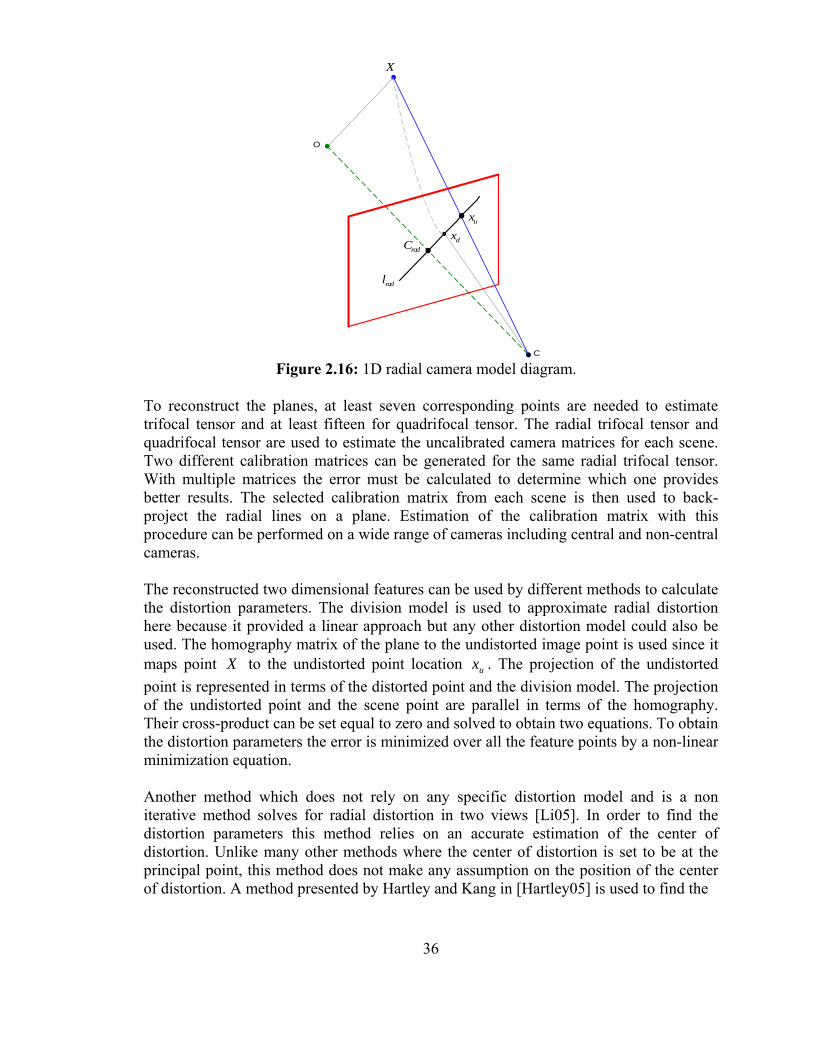
36

To reconstruct the planes, at least seven corresponding points are needed to estimate trifocal tensor and at least fifteen for quadrifocal tensor. The radial trifocal tensor and quadrifocal tensor are used to estimate the uncalibrated camera matrices for each scene. Two different calibration matrices can be generated for the same radial trifocal tensor. With multiple matrices the error must be calculated to determine which one provides better results. The selected calibration matrix from each scene is then used to back-project the radial lines on a plane. Estimation of the calibration matrix with this procedure can be performed on a wide range of cameras including central and non-central cameras. The reconstructed two dimensional features can be used by different methods to calculate the distortion parameters. The division model is used to approximate radial distortion here because it provided a linear approach but any other distortion model could also be used. The homography matrix of the plane to the undistorted image point is used since it maps point X to the undistorted point location ux . The projection of the undistorted point is represented in terms of the distorted point and the division model. The projection of the undistorted point and the scene point are parallel in terms of the homography. Their cross-product can be set equal to zero and solved to obtain two equations. To obtain the distortion parameters the error is minimized over all the feature points by a non-linear minimization equation. Another method which does not rely on any specific distortion model and is a non iterative method solves for radial distortion in two views [Li05]. In order to find the distortion parameters this method relies on an accurate estimation of the center of distortion. Unlike many other methods where the center of distortion is set to be at the principal point, this method does not make any assumption on the position of the center of distortion. A method presented by Hartley and Kang in [Hartley05] is used to find the

C

O

dxux

radC

radl

X

Figure 2.16: 1D radial camera model diagram.

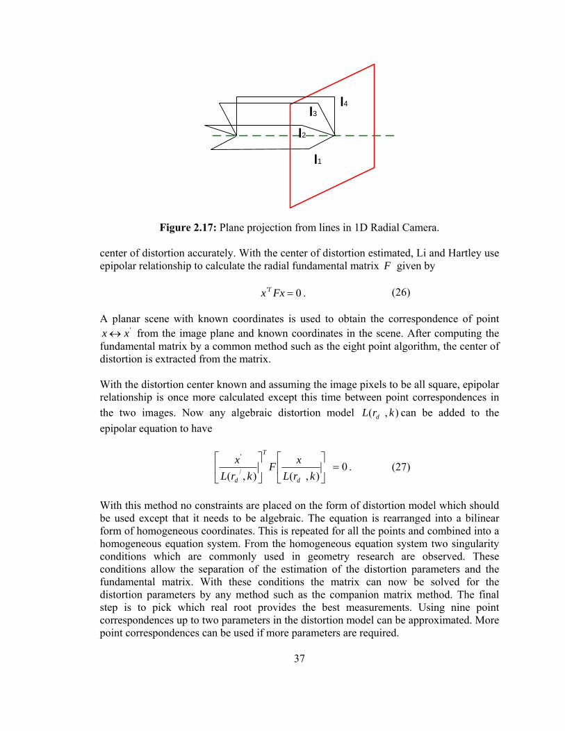
37

center of distortion accurately. With the center of distortion estimated, Li and Hartley use epipolar relationship to calculate the radial fundamental matrix F given by

0' =Fxx T . (26)

A planar scene with known coordinates is used to obtain the correspondence of point

'xx ↔ from the image plane and known coordinates in the scene. After computing the fundamental matrix by a common method such as the eight point algorithm, the center of distortion is extracted from the matrix. With the distortion center known and assuming the image pixels to be all square, epipolar relationship is once more calculated except this time between point correspondences in the two images. Now any algebraic distortion model ),( krL d can be added to the epipolar equation to have

0),(),( /

'

=⎥⎦

⎤⎢⎣

⎡⎥⎦

⎤⎢⎣

⎡

krLxF

krLx

d

T

d

. (27)

With this method no constraints are placed on the form of distortion model which should be used except that it needs to be algebraic. The equation is rearranged into a bilinear form of homogeneous coordinates. This is repeated for all the points and combined into a homogeneous equation system. From the homogeneous equation system two singularity conditions which are commonly used in geometry research are observed. These conditions allow the separation of the estimation of the distortion parameters and the fundamental matrix. With these conditions the matrix can now be solved for the distortion parameters by any method such as the companion matrix method. The final step is to pick which real root provides the best measurements. Using nine point correspondences up to two parameters in the distortion model can be approximated. More point correspondences can be used if more parameters are required.

l1

l2

l3l4

Figure 2.17: Plane projection from lines in 1D Radial Camera.

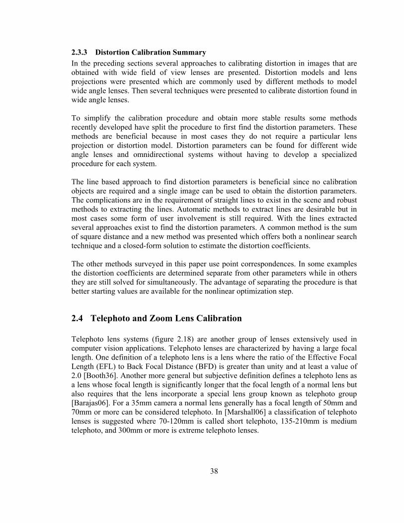
38

2.3.3 Distortion Calibration Summary In the preceding sections several approaches to calibrating distortion in images that are obtained with wide field of view lenses are presented. Distortion models and lens projections were presented which are commonly used by different methods to model wide angle lenses. Then several techniques were presented to calibrate distortion found in wide angle lenses. To simplify the calibration procedure and obtain more stable results some methods recently developed have split the procedure to first find the distortion parameters. These methods are beneficial because in most cases they do not require a particular lens projection or distortion model. Distortion parameters can be found for different wide angle lenses and omnidirectional systems without having to develop a specialized procedure for each system. The line based approach to find distortion parameters is beneficial since no calibration objects are required and a single image can be used to obtain the distortion parameters. The complications are in the requirement of straight lines to exist in the scene and robust methods to extracting the lines. Automatic methods to extract lines are desirable but in most cases some form of user involvement is still required. With the lines extracted several approaches exist to find the distortion parameters. A common method is the sum of square distance and a new method was presented which offers both a nonlinear search technique and a closed-form solution to estimate the distortion coefficients. The other methods surveyed in this paper use point correspondences. In some examples the distortion coefficients are determined separate from other parameters while in others they are still solved for simultaneously. The advantage of separating the procedure is that better starting values are available for the nonlinear optimization step.

2.4 Telephoto and Zoom Lens Calibration Telephoto lens systems (figure 2.18) are another group of lenses extensively used in computer vision applications. Telephoto lenses are characterized by having a large focal length. One definition of a telephoto lens is a lens where the ratio of the Effective Focal Length (EFL) to Back Focal Distance (BFD) is greater than unity and at least a value of 2.0 [Booth36]. Another more general but subjective definition defines a telephoto lens as a lens whose focal length is significantly longer that the focal length of a normal lens but also requires that the lens incorporate a special lens group known as telephoto group [Barajas06]. For a 35mm camera a normal lens generally has a focal length of 50mm and 70mm or more can be considered telephoto. In [Marshall06] a classification of telephoto lenses is suggested where 70-120mm is called short telephoto, 135-210mm is medium telephoto, and 300mm or more is extreme telephoto lenses.

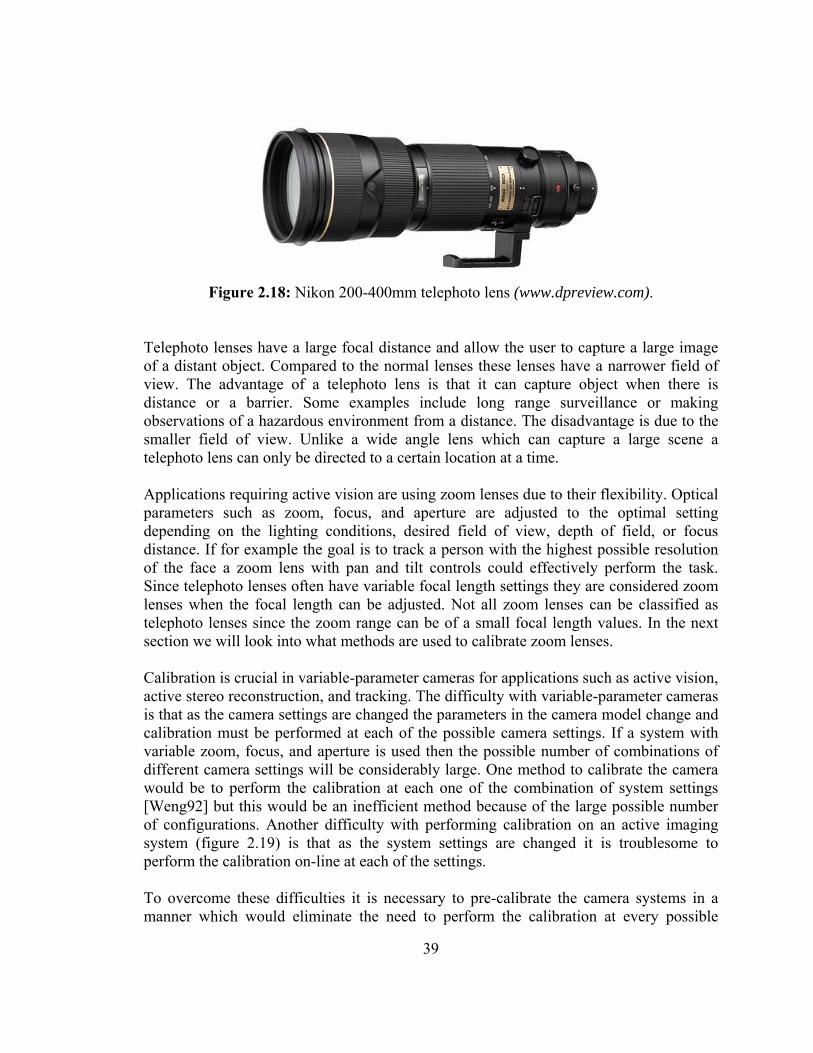
39

Telephoto lenses have a large focal distance and allow the user to capture a large image of a distant object. Compared to the normal lenses these lenses have a narrower field of view. The advantage of a telephoto lens is that it can capture object when there is distance or a barrier. Some examples include long range surveillance or making observations of a hazardous environment from a distance. The disadvantage is due to the smaller field of view. Unlike a wide angle lens which can capture a large scene a telephoto lens can only be directed to a certain location at a time. Applications requiring active vision are using zoom lenses due to their flexibility. Optical parameters such as zoom, focus, and aperture are adjusted to the optimal setting depending on the lighting conditions, desired field of view, depth of field, or focus distance. If for example the goal is to track a person with the highest possible resolution of the face a zoom lens with pan and tilt controls could effectively perform the task. Since telephoto lenses often have variable focal length settings they are considered zoom lenses when the focal length can be adjusted. Not all zoom lenses can be classified as telephoto lenses since the zoom range can be of a small focal length values. In the next section we will look into what methods are used to calibrate zoom lenses. Calibration is crucial in variable-parameter cameras for applications such as active vision, active stereo reconstruction, and tracking. The difficulty with variable-parameter cameras is that as the camera settings are changed the parameters in the camera model change and calibration must be performed at each of the possible camera settings. If a system with variable zoom, focus, and aperture is used then the possible number of combinations of different camera settings will be considerably large. One method to calibrate the camera would be to perform the calibration at each one of the combination of system settings [Weng92] but this would be an inefficient method because of the large possible number of configurations. Another difficulty with performing calibration on an active imaging system (figure 2.19) is that as the system settings are changed it is troublesome to perform the calibration on-line at each of the settings. To overcome these difficulties it is necessary to pre-calibrate the camera systems in a manner which would eliminate the need to perform the calibration at every possible

Figure 2.18: Nikon 200-400mm telephoto lens (www.dpreview.com).

40

system configuration. Willson [Willson94] presented a comprehensive work which serves as the foundation for many resent developments in the area of zoom lens calibration [Ahmed00] [Chen00] [Collins99] [Li96] [Shih98] [Thirthala05c]. The suggested methodology is to perform the calibration at discrete camera settings over the entire range of camera settings. The parameter values from these discrete camera settings are compiled into a table. The table shows how each parameter changes as the camera settings are varied. Depending on the necessary accuracy and application some parameters can be considered constant as the camera settings are changed but this will hold true only for the particular camera being calibrated. The next step is to use the table to find parameter values at all of the possible camera settings. One method is to fit a function to the calibrated values but for some parameters it may be difficult to fit a function [Willson94]. Another approach is to use the table as a lookup table and use functional interpolation to calculate the values at intermediate settings [Li95] [Chen00]. The disadvantage of this approach is that sometimes this may produce higher errors in the results as compared to using a function. To eliminate the disadvantages a combination of the two methods can be used. In [Shih98] some parameters are stored in a look up table to be used for interpolation while for others a function is evaluated. Willson’s method uses the fixed camera model to perform the calibration at different camera settings and with the collected data he creates an adjustable camera model. The method consists of three steps:

1. Collection of calibration data at fixed camera settings across entire ranges of settings

2. Calibration of the fixed camera model at each of the camera settings. 3. Characterization of the relationships between the fixed camera model’s

parameters and the lens settings. The first step consists of collecting calibration data at discrete camera settings using Tsai’s calibration method and a planar calibration pattern. The range over which the calibration is performed can be varied depending on the desired imaging properties. The sampling frequency must be sufficiently high for each of the variable settings so that any variation in the parameters can be accurately modeled. The range over which the camera settings are varied are shown in the table 2.1. The sampling is done at 121 individual

Figure 2.19: Canon NU-700 Pan-Tilt head with 20x (4.2-84mm) zoom lens www.canon.ca.

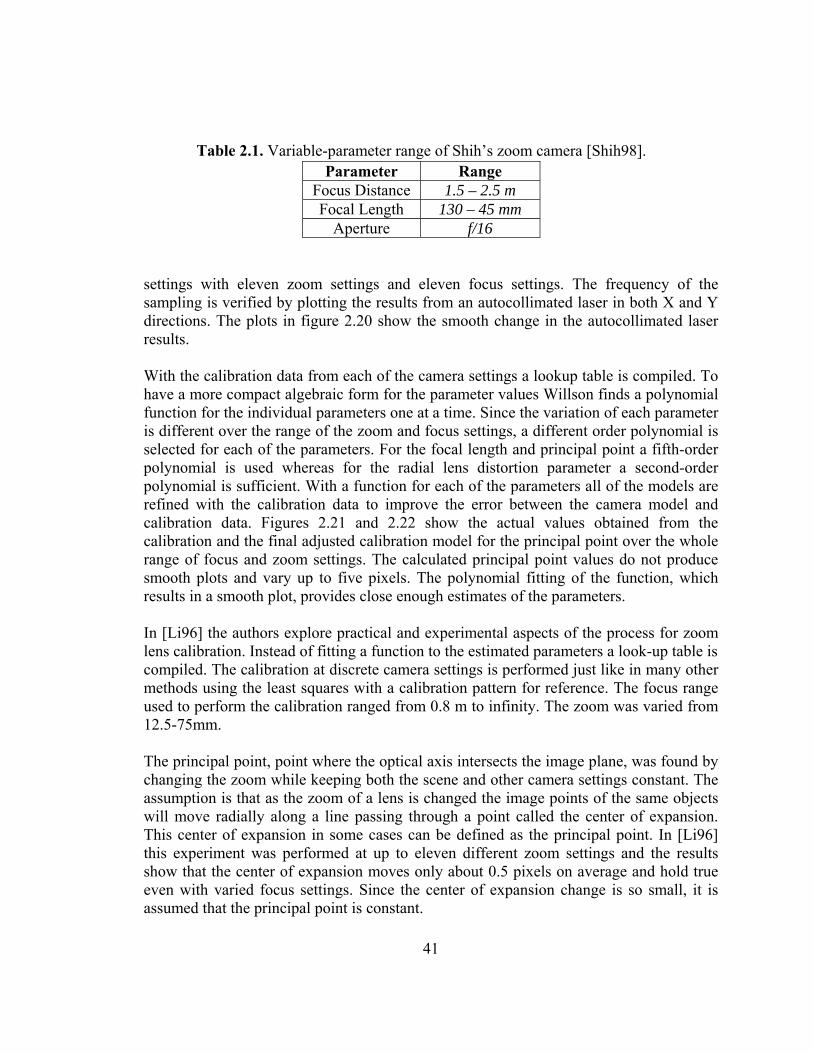
41

settings with eleven zoom settings and eleven focus settings. The frequency of the sampling is verified by plotting the results from an autocollimated laser in both X and Y directions. The plots in figure 2.20 show the smooth change in the autocollimated laser results. With the calibration data from each of the camera settings a lookup table is compiled. To have a more compact algebraic form for the parameter values Willson finds a polynomial function for the individual parameters one at a time. Since the variation of each parameter is different over the range of the zoom and focus settings, a different order polynomial is selected for each of the parameters. For the focal length and principal point a fifth-order polynomial is used whereas for the radial lens distortion parameter a second-order polynomial is sufficient. With a function for each of the parameters all of the models are refined with the calibration data to improve the error between the camera model and calibration data. Figures 2.21 and 2.22 show the actual values obtained from the calibration and the final adjusted calibration model for the principal point over the whole range of focus and zoom settings. The calculated principal point values do not produce smooth plots and vary up to five pixels. The polynomial fitting of the function, which results in a smooth plot, provides close enough estimates of the parameters. In [Li96] the authors explore practical and experimental aspects of the process for zoom lens calibration. Instead of fitting a function to the estimated parameters a look-up table is compiled. The calibration at discrete camera settings is performed just like in many other methods using the least squares with a calibration pattern for reference. The focus range used to perform the calibration ranged from 0.8 m to infinity. The zoom was varied from 12.5-75mm. The principal point, point where the optical axis intersects the image plane, was found by changing the zoom while keeping both the scene and other camera settings constant. The assumption is that as the zoom of a lens is changed the image points of the same objects will move radially along a line passing through a point called the center of expansion. This center of expansion in some cases can be defined as the principal point. In [Li96] this experiment was performed at up to eleven different zoom settings and the results show that the center of expansion moves only about 0.5 pixels on average and hold true even with varied focus settings. Since the center of expansion change is so small, it is assumed that the principal point is constant.

Table 2.1. Variable-parameter range of Shih’s zoom camera [Shih98].

Parameter Range Focus Distance 1.5 – 2.5 m Focal Length 130 – 45 mm

Aperture f/16

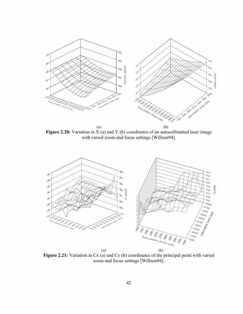
42

(a) (b) Figure 2.20: Variation in X (a) and Y (b) coordinates of an autocollimated laser image

with varied zoom and focus settings [Willson94].

(a) (b) Figure 2.21: Variation in Cx (a) and Cy (b) coordinates of the principal point with varied

zoom and focus settings [Willson94].

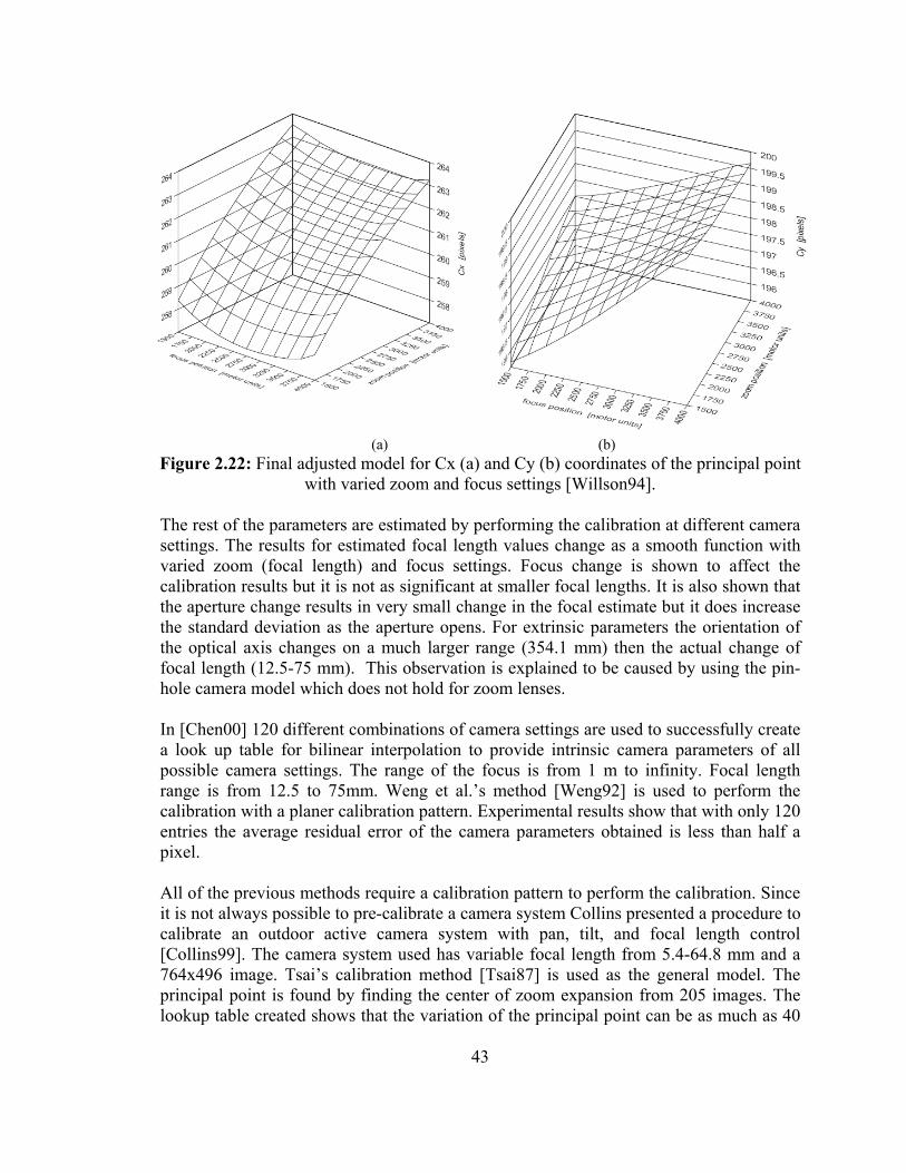
43

(a) (b)

Figure 2.22: Final adjusted model for Cx (a) and Cy (b) coordinates of the principal point with varied zoom and focus settings [Willson94].

The rest of the parameters are estimated by performing the calibration at different camera settings. The results for estimated focal length values change as a smooth function with varied zoom (focal length) and focus settings. Focus change is shown to affect the calibration results but it is not as significant at smaller focal lengths. It is also shown that the aperture change results in very small change in the focal estimate but it does increase the standard deviation as the aperture opens. For extrinsic parameters the orientation of the optical axis changes on a much larger range (354.1 mm) then the actual change of focal length (12.5-75 mm). This observation is explained to be caused by using the pin-hole camera model which does not hold for zoom lenses. In [Chen00] 120 different combinations of camera settings are used to successfully create a look up table for bilinear interpolation to provide intrinsic camera parameters of all possible camera settings. The range of the focus is from 1 m to infinity. Focal length range is from 12.5 to 75mm. Weng et al.’s method [Weng92] is used to perform the calibration with a planer calibration pattern. Experimental results show that with only 120 entries the average residual error of the camera parameters obtained is less than half a pixel. All of the previous methods require a calibration pattern to perform the calibration. Since it is not always possible to pre-calibrate a camera system Collins presented a procedure to calibrate an outdoor active camera system with pan, tilt, and focal length control [Collins99]. The camera system used has variable focal length from 5.4-64.8 mm and a 764x496 image. Tsai’s calibration method [Tsai87] is used as the general model. The principal point is found by finding the center of zoom expansion from 205 images. The lookup table created shows that the variation of the principal point can be as much as 40

44

pixels on the 764x496 image. The other intrinsic parameters are calibrated by pure rotation and using some Euclidean scene coordinates to determine the rotation and translation of the system. Telephoto lenses do not have a significant amount of pin-cushion distortion. Most of the time it is very hard if not impossible to visually see this distortion. For variable focal length lenses the effect of radial distortion decreases as the field of view is reduced. A vary-focal lens which at the lower end is considered to be a wide angle lens may have some distortion but as the focal length is increased the effect of the distortion decreases. In all of the zoom lens calibration methods very little attention is given to distortion. Ahmed and Farag suggest using some pre-calibration process to find the distortion parameters with the captured images, thus decoupling the process from finding other intrinsic parameters [Ahmed00]. To keep the complexity of the models low, most of the time a single coefficient is used to model radial lens distortion and no tangential distortion [Willson94] [Chen00]. Li [Li96] on the other hand used three radial distortion parameters and three tangential distortion parameters and showed that the third term in both radial and tangential equations were insignificant. He said the best approach is to use the model with two radial and tangential coefficients. Furthermore he showed that with varied camera settings on his system the distortion parameters did not change significantly and could be assumed to be constant. Another concern with variable-parameter cameras is the calibration pattern to be used. The orientation of the calibration pattern can have an effect on the calibration results [Li96]. With variable-parameter cameras another issue is that with a constant calibration pattern as the parameters change the field of view of the camera may reduce and not be able to capture the whole calibration pattern. In these cases the range over which the calibration can be performed is limited. Figure 2.23 shows that if a smaller calibration pattern is selected to cover the whole range of the camera settings the calibration pattern would appear much smaller at some settings and fit the whole field of view at others settings. The difference in the pattern size would affect the calibration results.

(a) (b) Figure 2.23: Calibration pattern with focal length of 70mm (a) and 210mm (b) with

Nikon 210mm Lens at 3m focus.

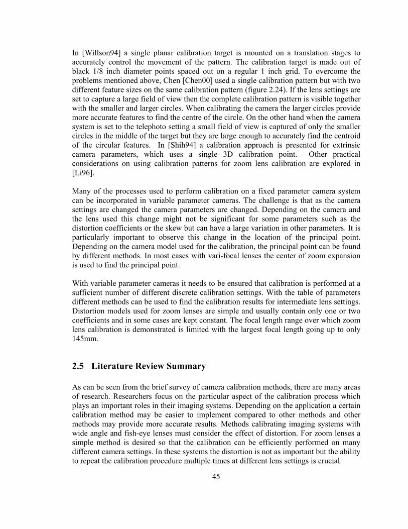
45

In [Willson94] a single planar calibration target is mounted on a translation stages to accurately control the movement of the pattern. The calibration target is made out of black 1/8 inch diameter points spaced out on a regular 1 inch grid. To overcome the problems mentioned above, Chen [Chen00] used a single calibration pattern but with two different feature sizes on the same calibration pattern (figure 2.24). If the lens settings are set to capture a large field of view then the complete calibration pattern is visible together with the smaller and larger circles. When calibrating the camera the larger circles provide more accurate features to find the centre of the circle. On the other hand when the camera system is set to the telephoto setting a small field of view is captured of only the smaller circles in the middle of the target but they are large enough to accurately find the centroid of the circular features. In [Shih94] a calibration approach is presented for extrinsic camera parameters, which uses a single 3D calibration point. Other practical considerations on using calibration patterns for zoom lens calibration are explored in [Li96]. Many of the processes used to perform calibration on a fixed parameter camera system can be incorporated in variable parameter cameras. The challenge is that as the camera settings are changed the camera parameters are changed. Depending on the camera and the lens used this change might not be significant for some parameters such as the distortion coefficients or the skew but can have a large variation in other parameters. It is particularly important to observe this change in the location of the principal point. Depending on the camera model used for the calibration, the principal point can be found by different methods. In most cases with vari-focal lenses the center of zoom expansion is used to find the principal point. With variable parameter cameras it needs to be ensured that calibration is performed at a sufficient number of different discrete calibration settings. With the table of parameters different methods can be used to find the calibration results for intermediate lens settings. Distortion models used for zoom lenses are simple and usually contain only one or two coefficients and in some cases are kept constant. The focal length range over which zoom lens calibration is demonstrated is limited with the largest focal length going up to only 145mm.

2.5 Literature Review Summary As can be seen from the brief survey of camera calibration methods, there are many areas of research. Researchers focus on the particular aspect of the calibration process which plays an important roles in their imaging systems. Depending on the application a certain calibration method may be easier to implement compared to other methods and other methods may provide more accurate results. Methods calibrating imaging systems with wide angle and fish-eye lenses must consider the effect of distortion. For zoom lenses a simple method is desired so that the calibration can be efficiently performed on many different camera settings. In these systems the distortion is not as important but the ability to repeat the calibration procedure multiple times at different lens settings is crucial.

46

(a)

(b)

(c) Figure 2.24: Complete calibration pattern (a) with images captured at wide-angle

setting (b) and telephoto setting (c).

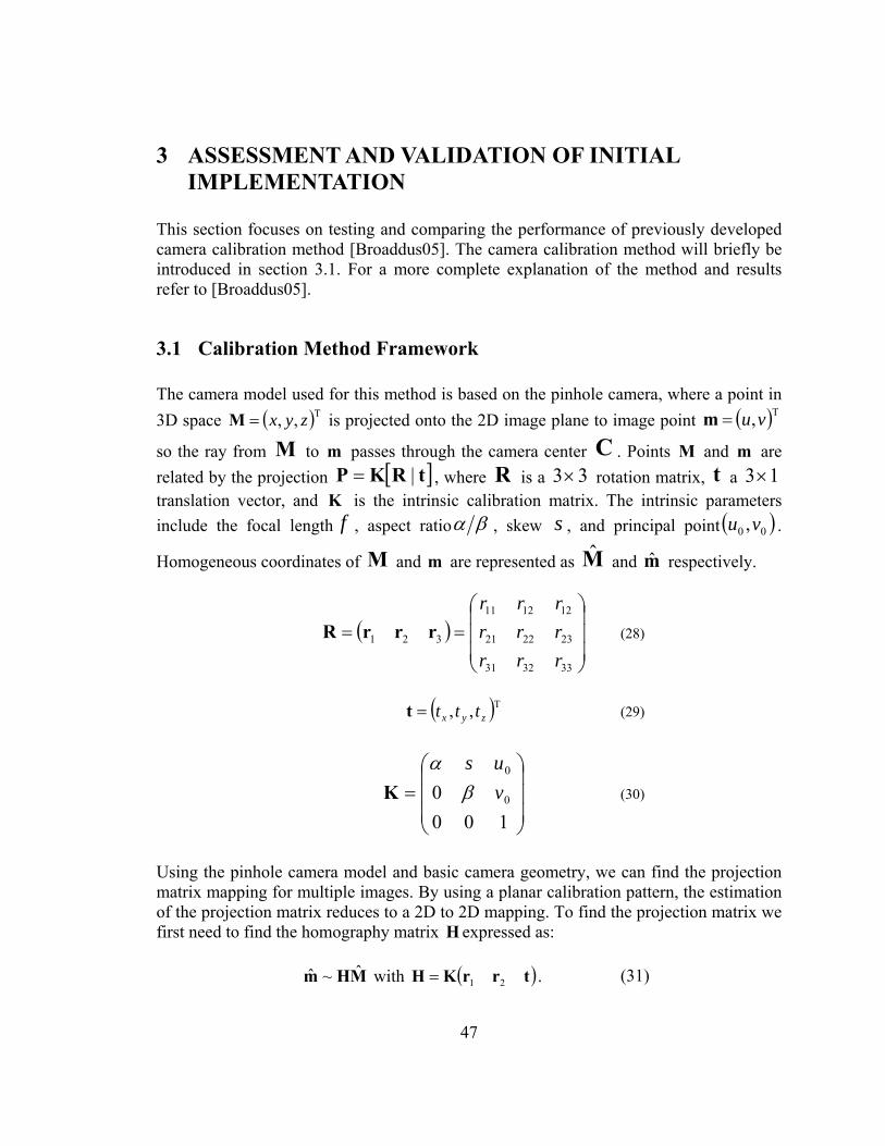
47

3 ASSESSMENT AND VALIDATION OF INITIAL IMPLEMENTATION

This section focuses on testing and comparing the performance of previously developed camera calibration method [Broaddus05]. The camera calibration method will briefly be introduced in section 3.1. For a more complete explanation of the method and results refer to [Broaddus05].

3.1 Calibration Method Framework The camera model used for this method is based on the pinhole camera, where a point in 3D space ( )T,, zyx=M is projected onto the 2D image plane to image point ( )T,vu=m

so the ray from M to m passes through the camera center C . Points M and m are related by the projection [ ]tRKP |= , where R is a 33× rotation matrix, t a 13× translation vector, and K is the intrinsic calibration matrix. The intrinsic parameters include the focal length f , aspect ratio βα , skew s , and principal point ( )00 ,vu .

Homogeneous coordinates of M and m are represented as M̂ and m̂ respectively.

( )⎟⎟⎟

⎠

⎞

⎜⎜⎜

⎝

⎛==

333231

232221

121211

321

rrrrrrrrr

rrrR (28)

( )T,, zyx ttt=t (29)

⎟⎟⎟

⎠

⎞

⎜⎜⎜

⎝

⎛=

1000 0

0

vus

βα

K (30)

Using the pinhole camera model and basic camera geometry, we can find the projection matrix mapping for multiple images. By using a planar calibration pattern, the estimation of the projection matrix reduces to a 2D to 2D mapping. To find the projection matrix we first need to find the homography matrix H expressed as:

MHm ˆ~ˆ with ( )trrKH 21= . (31)

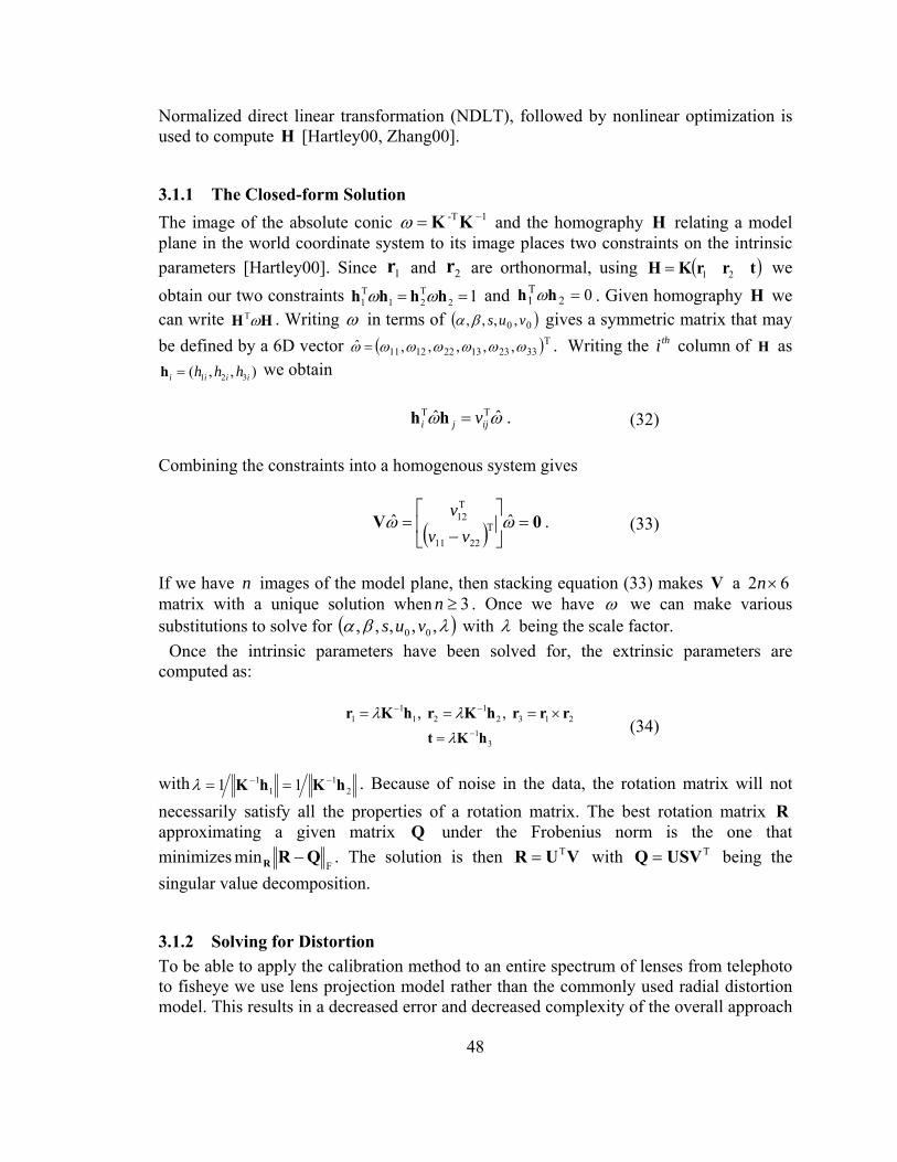
48

Normalized direct linear transformation (NDLT), followed by nonlinear optimization is used to compute H [Hartley00, Zhang00].

3.1.1 The Closed-form Solution The image of the absolute conic 1-T −= KKω and the homography H relating a model plane in the world coordinate system to its image places two constraints on the intrinsic parameters [Hartley00]. Since 1r and 2r are orthonormal, using ( )trrKH 21= we obtain our two constraints 12

T21

T1 == hhhh ωω and 02

T1 =hh ω . Given homography H we

can write HH ωT . Writing ω in terms of ( )00 ,,,, vusβα gives a symmetric matrix that may be defined by a 6D vector ( )T332313221211 ,,,,,ˆ ωωωωωωω = . Writing the thi column of H as

1 2 3( , , )i i i ih h h=h we obtain

ωω ˆˆ TTijji v=hh . (32)

Combining the constraints into a homogenous system gives

( ) 0V =⎥⎦

⎤⎢⎣

⎡

−= ωω ˆˆ T

2211

T12

vvv

. (33)

If we have n images of the model plane, then stacking equation (33) makes V a 62 ×n matrix with a unique solution when 3≥n . Once we have ω we can make various substitutions to solve for ( )λβα ,,,,, 00 vus with λ being the scale factor.

Once the intrinsic parameters have been solved for, the extrinsic parameters are computed as:

2132

121

11 , , rrrhKrhKr ×=== −− λλ

31hKt −= λ (34)

with 2

11

1 11 hKhK −− ==λ . Because of noise in the data, the rotation matrix will not necessarily satisfy all the properties of a rotation matrix. The best rotation matrix R approximating a given matrix Q under the Frobenius norm is the one that minimizes

Fmin QRR − . The solution is then VUR T= with TUSVQ = being the

singular value decomposition.

3.1.2 Solving for Distortion To be able to apply the calibration method to an entire spectrum of lenses from telephoto to fisheye we use lens projection model rather than the commonly used radial distortion model. This results in a decreased error and decreased complexity of the overall approach

49

as compared to modeling radial distortion. Standard cameras are built to follow a perspective projection. However, perspective projection has an asymptote at 180° FOV which makes it extremely difficult to build a rectilinear lens above 100° FOV. Other types of projections have been proposed [Kannala04] to overcome these limitation and are listed in Table 3.1. In practice, real cameras do not exactly follow the projections in Table 3.1. A polynomial is used to approximate the real lens projection in the form:

( ) ( )…++== ∑=

− 321

1

12 φκφκφκφ ffrp

i

ii . (35)

Once a solution has been computed for the calibration matrix, rotation matrix and translation vector, a least-squares solution to p lens projection coefficients

( )T21 ,, pκκκ …=κ is computed. In optical systems the centers of lens elements are not strictly collinear and are subject to various amounts of decentering distortion [Tsai87]. This distortion has both radial and tangential components and can be modeled as:

( )( )( )( )( )( )⎟⎟⎠

⎞⎜⎜⎝

⎛

++++++++++

=……

3432

221

343

2221

1212

rruvvrrruruv

ρρρρρρρρ

∆d (36)

with q decentering coefficients ( )qρρρ …,, 21=ρ . Since decentering distortion is usually small, initial estimates are set to zero and then later optimized with other parameters.

3.1.3 Final Parameter Optimization Once the close-from solutions to the camera parameters are computed, including the distortion coefficients, the results are refined using maximum likelihood estimation (MLE) by minimizing equation:

Table 3.1. Commonly used types of lens projections. Name Formula 1 Perspective φtanfr = 2 Stereographic ( )2tan2 φfr =

3 Equisolid ( )2sin2 φfr = 4 Orthogonal φsinfr =

50

( )2

1 1,,,,,∑∑

= =

−n

i

m

jjiiij MρκtRKmm , (37)

where ( )jii MρκtRKm ,,,,, is the projection of points jM in image i and ijm is the coordinates of point on the image plane. From the experiments, Broaddus [Broaddus05] showed that, as the lens projection deviates from the perspective projection, alternating between refining ( )tRK ,, and ( )ρκ, produces significantly better results. Levenberg-Marquardt algorithm is used to perform MLE. The complete calibration method is outlined below.

1. Acquire at least three images of a planar calibration pattern at different camera orientations and translations.

2. Detect and match features of the calibration pattern in the images. 3. Estimate the homographies relating the model plane to the images. 4. Estimate the intrinsic and extrinsic parameters. 5. Estimate the coefficients of the lens projection. 6. Initialize the decentering distortion coefficients to zero. 7. Refine all parameters using MLE with bundle adjustment.

3.1.4 Distortion Model Selection Distortion model selection is the task of choosing the best model for a given system when several competing models can represent the distortion. Even though any model can be incorporated into the algorithm introduced above, the use of the most fitting and concise model will provide both better accuracy and reduced computational complexity. In most cases the model with more degrees of freedom will fit the data closer than other less complex models but higher order terms in the polynomial models may cause numerical instability [Tsai86] [Wei94] [Zhang00]. To help with stability and since higher order terms in the radial distortion model are comparatively insignificant in some systems, the number of distortion coefficients are kept low when modeling standard cameras [Tsai86] [Wei94] but higher order terms may be necessary when modeling wide-angle lenses. Including additional distortion parameters also increases the computation complexity and time of camera calibration. Figure 3.1 shows the relative computation time of complete camera calibration with different number of distortion coefficients. The computation time increases with the addition of both radial and tangential coefficients. The increase in computation time will be dependent on the distortion model complexity, amount of distortion, size of data set, and nonlinear optimization criteria. The goal is to develop an automatic model selection criterion based on a quantitative measure which will select the model with a reduced number of coefficients without sacrificing accuracy. Akaike laid the foundation for statistical model selection by

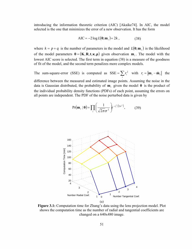
51

introducing the information theoretic criterion (AIC) [Akaike74]. In AIC, the model selected is the one that minimizes the error of a new observation. It has the form

( ) kL i 2;log2AIC +−= mθ , (38) where qpk += is the number of parameters in the model and ( )iL mθ; is the likelihood of the model parameters ( )ρκtRKθ ,,,,= given observation im . The model with the lowest AIC score is selected. The first term in equation (38) is a measure of the goodness of fit of the model, and the second term penalizes more complex models. The sum-square-error (SSE) is computed as ∑=

iir2SSE with iiir mm −= the

difference between the measured and estimated image points. Assuming the noise in the data is Gaussian distributed, the probability of im given the model θ is the product of the individual probability density functions (PDFs) of each point, assuming the errors on all points are independent. The PDF of the noise perturbed data is given by

( ) ( )22 222

1|Pr σ

σπir

ii e −∏ ⎟⎟

⎠

⎞⎜⎜⎝

⎛=θm , (39)

01

23

4

1

2

3

420

40

60

80

100

120

140

160

Number Tangential Coef.Number Radial Coef.

Com

puta

tion

Tim

e [m

in]

(a)

Figure 3.1: Computation time for Zhang’s data using the lens projection model. Plot shows the computation time as the number of radial and tangential coefficients are

changed on a 640x480 image.

52

where 2σ is the variance of noise [Gheissari03]. The log-likelihood of the model parameters θ given the observations im is then:

( ) ( ) 22

1log ; arg log Pr | constant.2i i i

iL r

σ⎡ ⎤= = − +⎣ ⎦ ∑

θθ m m θ (40)

The maximum log-likelihood estimate (MLE) is the set of parameters θ that maximizes ( )iL mθ;log . We observe that minimizing the SSE is equivalent to maximizing the log-likelihood, which is in-turn equivalent to maximizing the likelihood of the model parametersθ . Therefore, by substituting equation (40) into equation (38) and simplifying, we can write AIC in the following form:

kri

i 21AIC 22 += ∑σ

. (41)

We use the formulation in [Gheissari03] to calculate the variance 2σ of unknown Gaussian noise:

( )kNri

iˆ22 −=∑σ , (42)

where N is the number of samples and k̂ is the number of coefficients of the most complex competing model. In summary, using the proposed distortion model, a variety of ( , )p q distortion models are fit to the data. Then one of the criteria listed in Table 3.2 is used to select the distortion model. The selection of which criterion to used should be determined by the application, data size, noise, and model library [Gheissari03].

Table 3.2. Model selection criteria.

Name Formula AIC [Akaike74] ( ) kL i 2;log2 +− mθ

MDL [Rissanen78] ( ) NkL i log21;log2 +− mθ

BIC [Schwarz78] ( ) NkL i log2;log2 +− mθ SSD [Rissanen78] ( ) ( )[ ] ( )1log2242log;log2 ++++− kNkL imθ

CAIC [Bozdogan87] ( ) ( )1log;log2 ++− NkL imθ

53

3.2 Evaluation of Distortion Model Complexity Selection The proposed distortion model complexity selection was previously used to automatically select the best distortion from competing distortion models using several real data sets [Broaduss05]. Two deferent polynomial distortion models were used. The Lens Projection with Decentering Distortion (LPDD) model and the Radial Distortion with Decentering Distortion (RDDD) model. With the automatically selected distortion model complexities it was shown that using the LPDD model we can use a less complex distortion model as we would have to using the RDDD model. To provide verification and support for these results we further test the performance of the distortion model complexity selection method. We first verify the performance of automatic distortion model selection by using ground truth data. We generate synthetic data using a particular distortion model and then perform automatic distortion model selection to observe what distortion model is selected. We also show the robustness of the model complexity selection by adding noise to the synthetic data and observing how that influences the results. In generating synthetic data and performing distortion model selection we must keep in mind comments made by Gheissari and Bab-Hadiashar [Gheissari03]. In their article they compare the performance of different model selection criteria. They say that many factors affect the suitability of criteria for employment in computer vision applications. They suggest that the most important factors, of which we also observed the significance in our implementation, are the application, data size, noise, and model library. The application which in our case is modeling lens distortion, determines the physical constraints and mathematical models. The data size which includes the size of the image is shown by Gheissari and Bab-Hadiashar to significantly change the performance of model selection criterion. In our implementation the data size includes the size of the image, number of images, and the number of points in the calibration grid. Since this is an important factor and which we can control in generating our synthetic data we selected values which were similar to values provided with real data. In real data we used imaged that included sizes of 800x600 and 640x480. Our calibration pattern contained 64 control points and we generally used eight images to perform the calibration. Since the scale and distribution of noise effects the performance of model selection criteria, we also tested the performance for a varied range of noise levels. The other important factor is the characteristics of the model library. In generating synthetic data this may be the most important factor. The model library includes the various competing models from which the best model is selected. In our application the model library includes the various distortion models with varying number of radial and tangential distortion coefficients. If the different competing models are very similar it may be difficult to accurately select the correct model. In the synthetic data generated for different order distortion models the distortion generated by the different number of coefficients should not produce significantly similar lens distortion but on the other hand

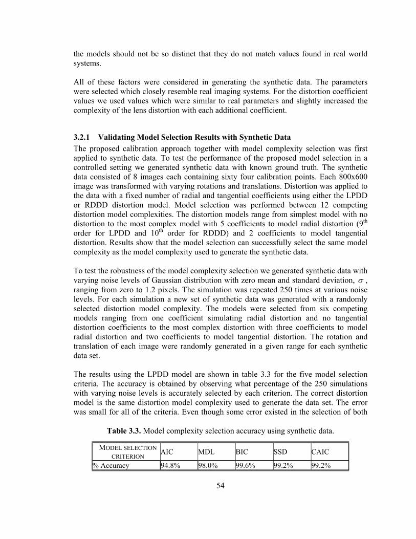
54

the models should not be so distinct that they do not match values found in real world systems. All of these factors were considered in generating the synthetic data. The parameters were selected which closely resemble real imaging systems. For the distortion coefficient values we used values which were similar to real parameters and slightly increased the complexity of the lens distortion with each additional coefficient.

3.2.1 Validating Model Selection Results with Synthetic Data The proposed calibration approach together with model complexity selection was first applied to synthetic data. To test the performance of the proposed model selection in a controlled setting we generated synthetic data with known ground truth. The synthetic data consisted of 8 images each containing sixty four calibration points. Each 800x600 image was transformed with varying rotations and translations. Distortion was applied to the data with a fixed number of radial and tangential coefficients using either the LPDD or RDDD distortion model. Model selection was performed between 12 competing distortion model complexities. The distortion models range from simplest model with no distortion to the most complex model with 5 coefficients to model radial distortion (9th order for LPDD and 10th order for RDDD) and 2 coefficients to model tangential distortion. Results show that the model selection can successfully select the same model complexity as the model complexity used to generate the synthetic data. To test the robustness of the model complexity selection we generated synthetic data with varying noise levels of Gaussian distribution with zero mean and standard deviation, σ , ranging from zero to 1.2 pixels. The simulation was repeated 250 times at various noise levels. For each simulation a new set of synthetic data was generated with a randomly selected distortion model complexity. The models were selected from six competing models ranging from one coefficient simulating radial distortion and no tangential distortion coefficients to the most complex distortion with three coefficients to model radial distortion and two coefficients to model tangential distortion. The rotation and translation of each image were randomly generated in a given range for each synthetic data set. The results using the LPDD model are shown in table 3.3 for the five model selection criteria. The accuracy is obtained by observing what percentage of the 250 simulations with varying noise levels is accurately selected by each criterion. The correct distortion model is the same distortion model complexity used to generate the data set. The error was small for all of the criteria. Even though some error existed in the selection of both

Table 3.3. Model complexity selection accuracy using synthetic data.

MODEL SELECTION CRITERION AIC MDL BIC SSD CAIC

% Accuracy 94.8% 98.0% 99.6% 99.2% 99.2%

55

radial and tangential coefficients most of the error was in the selection of tangential coefficients. The highest accuracy was achieved with the BIC criterion. The lowest accuracy was achieved with the AIC criterion since the second term which penalizes the model complexity does not take into account the number of samples in the model. We also verified the performance of our method with published RDDD distortion coefficient values in [El-Melegy03]. Even though this is a simpler approach it is yet another test in a controlled setting to insure the accurate selection of the best distortion model. Several 320x242 images with 64 control point were generated with various rotations and translation. Radial distortion was applied using the radial polynomial model with two coefficient values of [k1=20x10e-6, k2=30x10e-9]. Our method successfully performed the correct model complexity selection between the three competing models when these values were used to generate the synthetic data.

3.2.2 Model Selection Results with Real Data For experimental results on distortion model complexity selection with real data we repeated the experiment performed in [Broaddus05] and extended it to include telephoto lens results. Here we will show the results for all of the criteria and plots for the MDL criterion. We applied the calibration algorithm with distortion model selection to five cameras: (1) 210mm Nikon Vari-focal Lens, (2) PULNiX CCD camera with 6mm lens [2], (3) IQEye3 with a FUJINON 1.4-3.1 mm lens set to wide angle, and a Nikon fisheye FC-E8 lens set to two different zoom to produce a (4) full frame fisheye (FOV of 180° across the diagonal) and (5) circular fisheye (FOV of 180° in all directions). Tables 3.4 and 3.5 show the results for distortion model complexity selection using real data. The graphs in figure 3.2 show the distortion model complexity selection for MDL criterion. The plots show the complexity of the overall distortion model and the complexity of only the radial distortion as they are selected by the RDDD and LPDD models.

3.2.3 Which criteria should be used? Real data results show that different criteria do not always select the same model. The reason for the selection of different distortion models is due to the different weight assigned to the second term in the five criteria. The reason for the different cost functions is due to the assumptions made when deriving these criteria. In some cases even though different assumptions were used the final criteria are very similar. All of the criteria share the assumption that the number of samples is much larger than the number of estimated model parameters but the difference is how the measure is penalized for having complex models. The measure is penalized depending on the relation between the number of samples and the complexity of the models.

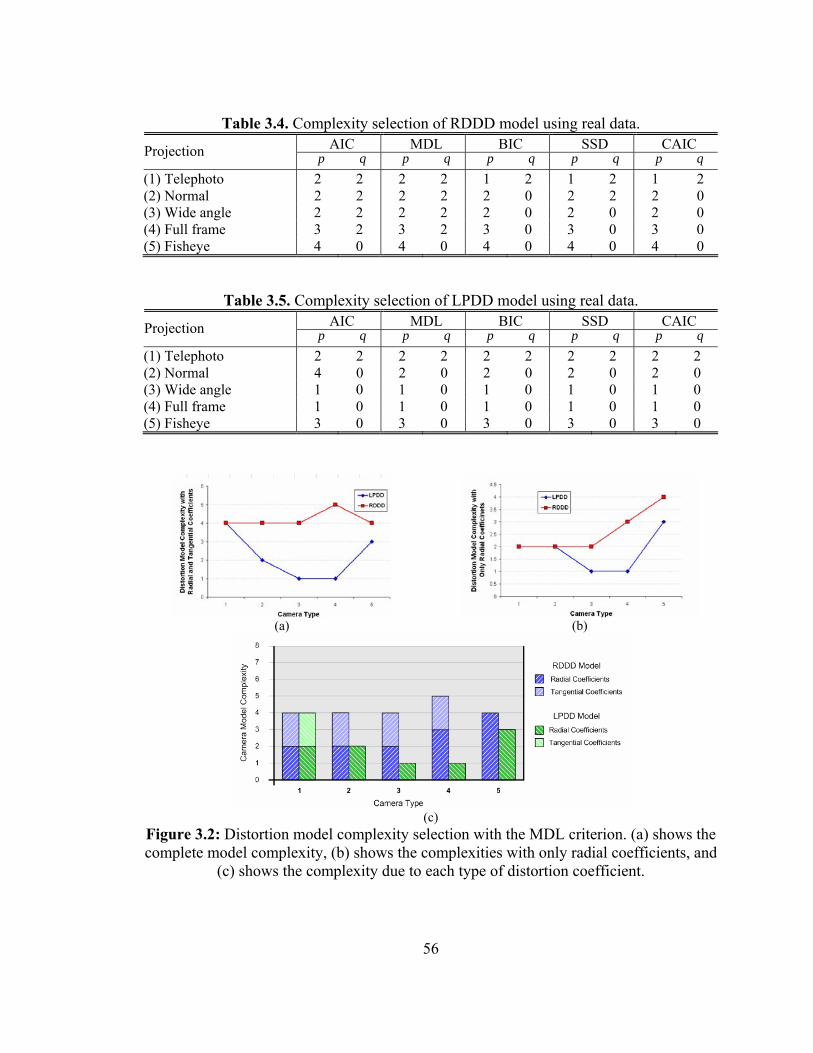
56

Table 3.4. Complexity selection of RDDD model using real data.

AIC MDL BIC SSD CAIC Projection p q p q p q p q p q (1) Telephoto 2 2 2 2 1 2 1 2 1 2 (2) Normal 2 2 2 2 2 0 2 2 2 0 (3) Wide angle 2 2 2 2 2 0 2 0 2 0 (4) Full frame 3 2 3 2 3 0 3 0 3 0 (5) Fisheye 4 0 4 0 4 0 4 0 4 0

Table 3.5. Complexity selection of LPDD model using real data. AIC MDL BIC SSD CAIC Projection p q p q p q p q p q

(1) Telephoto 2 2 2 2 2 2 2 2 2 2 (2) Normal 4 0 2 0 2 0 2 0 2 0 (3) Wide angle 1 0 1 0 1 0 1 0 1 0 (4) Full frame 1 0 1 0 1 0 1 0 1 0 (5) Fisheye 3 0 3 0 3 0 3 0 3 0

(a)

(b)

(c)

Figure 3.2: Distortion model complexity selection with the MDL criterion. (a) shows the complete model complexity, (b) shows the complexities with only radial coefficients, and

(c) shows the complexity due to each type of distortion coefficient.

57

An example of the dependency on the sample size is that if the sample size is small then MDL, BIC, SSD, and CAIC will underestimate the model whereas AIC will overestimate the model complexity. AIC also should not be used for data with significantly larger number of samples compared to the number of model parameters because as the number of samples becomes significantly large the second term becomes insignificant. These observations apply to our implementation because with our data sets the numbers of parameters vary by a small amount but the number of samples can vary from very small numbers to very large numbers. We may use only a few distortion parameters and several calibration images or we can use very complex distortion models and use many images with large calibration patterns. Since AIC is greatly influenced by the sample size, we abstain from using this criterion. These observations also explain the poor performance of AIC criterion on synthetic data where AIC performed the worst from among the five criteria. Criteria MDL, BIC, SSD, and CAIC were proposed after AIC and were developed for particular applications or to address the limitation of preceding criteria. MDL which represents the minimum description length select the least complex model that sufficiently describes the observation. SSD finds the shortest description length and shares similar fundamental principals as MDL criterion. BIC which uses Bayesian conditional probability selects the model that maximizes the conditional probability of the data by priori information. In our application the priori information is provided by the closed from solution to the camera parameters. CAIC was proposed to address the tendency of AIC to overestimate the model complexity by considering the number of samples provided by the data [Gheissari03]. Using the assumptions and the results with synthetic data we can justify the use of MDL, BIC, SSD, and CAIC criteria for distortion model complexity selection. AIC is not used because it is depended on the size of the data for the number of samples and the number of parameters in the model. For our application since higher complexity models increase computation time and we are not trying to predict the model but are looking for the least model complexity that sufficiently models the distortion, we use MDL to select the model complexity. MDL is a good estimate of the least complex model that provides us with a model that will efficiently model the distortion. This is consistent with the observation by Broaddus in [Broaddus05] where he says, “MDL was chosen over the other criteria to generate these plots [results] because it always selected a complexity less than or equal to that of the other criteria, without sacrificing a significantly lower error.”

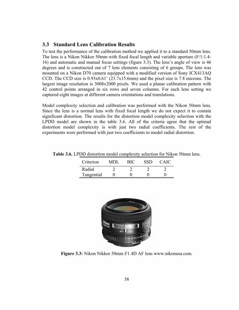
58

3.3 Standard Lens Calibration Results To test the performance of the calibration method we applied it to a standard 50mm lens. The lens is a Nikon Nikkor 50mm with fixed focal length and variable aperture (F/1:1.4-16) and automatic and manual focus settings (figure 3.3). The lens’s angle of view is 46 degrees and is constructed out of 7 lens elements consisting of 6 groups. The lens was mounted on a Nikon D70 camera equipped with a modified version of Sony ICX413AQ CCD. The CCD size is 0.93x0.61’ (23.7x15.6mm) and the pixel size is 7.8 microns. The largest image resolution is 3008x2000 pixels. We used a planar calibration pattern with 42 control points arranged in six rows and seven columns. For each lens setting we captured eight images at different camera orientations and translations. Model complexity selection and calibration was performed with the Nikon 50mm lens. Since the lens is a normal lens with fixed focal length we do not expect it to contain significant distortion. The results for the distortion model complexity selection with the LPDD model are shown in the table 3.6. All of the criteria agree that the optimal distortion model complexity is with just two radial coefficients. The rest of the experiments were performed with just two coefficients to model radial distortion.

Table 3.6. LPDD distortion model complexity selection for Nikon 50mm lens.

Criterion MDL BIC SSD CAIC Radial 2 2 2 2 Tangential 0 0 0 0

Figure 3.3: Nikon Nikkor 50mm f/1.4D AF lens www.nikonusa.com.

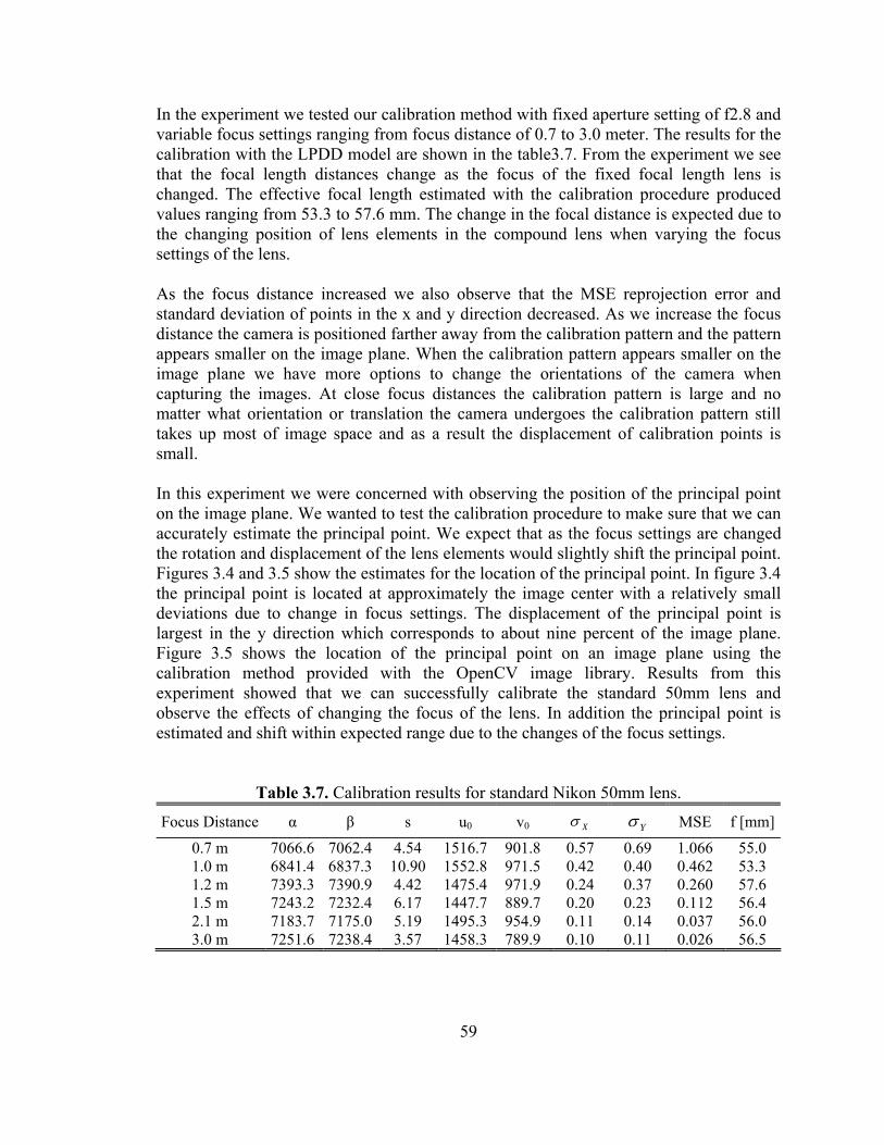
59

In the experiment we tested our calibration method with fixed aperture setting of f2.8 and variable focus settings ranging from focus distance of 0.7 to 3.0 meter. The results for the calibration with the LPDD model are shown in the table3.7. From the experiment we see that the focal length distances change as the focus of the fixed focal length lens is changed. The effective focal length estimated with the calibration procedure produced values ranging from 53.3 to 57.6 mm. The change in the focal distance is expected due to the changing position of lens elements in the compound lens when varying the focus settings of the lens. As the focus distance increased we also observe that the MSE reprojection error and standard deviation of points in the x and y direction decreased. As we increase the focus distance the camera is positioned farther away from the calibration pattern and the pattern appears smaller on the image plane. When the calibration pattern appears smaller on the image plane we have more options to change the orientations of the camera when capturing the images. At close focus distances the calibration pattern is large and no matter what orientation or translation the camera undergoes the calibration pattern still takes up most of image space and as a result the displacement of calibration points is small. In this experiment we were concerned with observing the position of the principal point on the image plane. We wanted to test the calibration procedure to make sure that we can accurately estimate the principal point. We expect that as the focus settings are changed the rotation and displacement of the lens elements would slightly shift the principal point. Figures 3.4 and 3.5 show the estimates for the location of the principal point. In figure 3.4 the principal point is located at approximately the image center with a relatively small deviations due to change in focus settings. The displacement of the principal point is largest in the y direction which corresponds to about nine percent of the image plane. Figure 3.5 shows the location of the principal point on an image plane using the calibration method provided with the OpenCV image library. Results from this experiment showed that we can successfully calibrate the standard 50mm lens and observe the effects of changing the focus of the lens. In addition the principal point is estimated and shift within expected range due to the changes of the focus settings.

Table 3.7. Calibration results for standard Nikon 50mm lens.

Focus Distance α β s u0 v0 Xσ Yσ MSE f [mm]

0.7 m 7066.6 7062.4 4.54 1516.7 901.8 0.57 0.69 1.066 55.0 1.0 m 6841.4 6837.3 10.90 1552.8 971.5 0.42 0.40 0.462 53.3 1.2 m 7393.3 7390.9 4.42 1475.4 971.9 0.24 0.37 0.260 57.6 1.5 m 7243.2 7232.4 6.17 1447.7 889.7 0.20 0.23 0.112 56.4 2.1 m 7183.7 7175.0 5.19 1495.3 954.9 0.11 0.14 0.037 56.0 3.0 m 7251.6 7238.4 3.57 1458.3 789.9 0.10 0.11 0.026 56.5

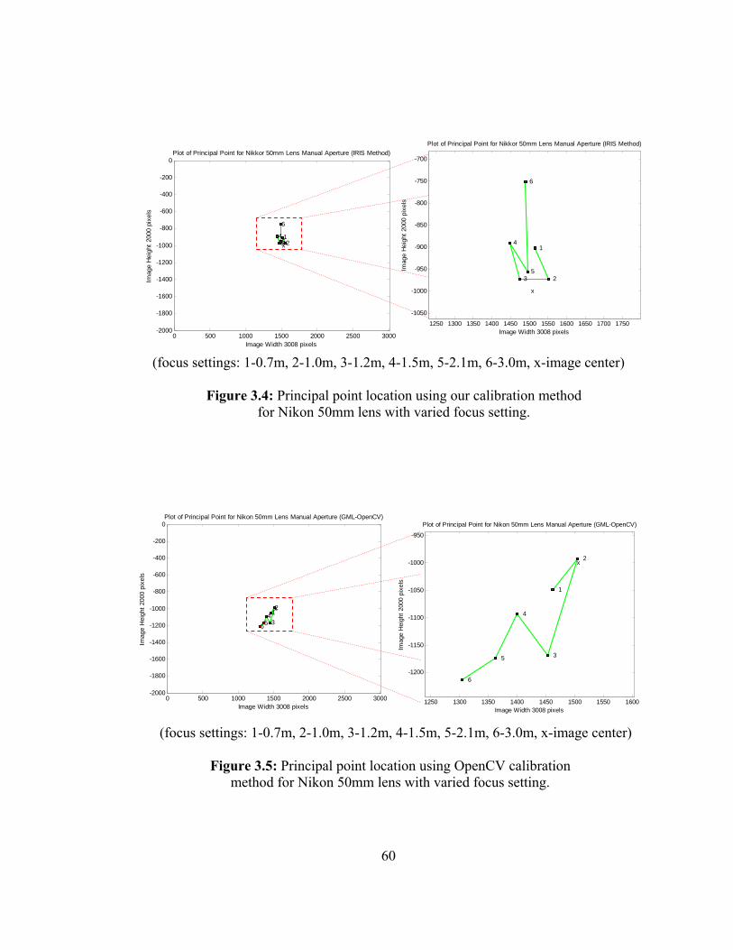
60

(focus settings: 1-0.7m, 2-1.0m, 3-1.2m, 4-1.5m, 5-2.1m, 6-3.0m, x-image center)

Figure 3.4: Principal point location using our calibration method for Nikon 50mm lens with varied focus setting.

(focus settings: 1-0.7m, 2-1.0m, 3-1.2m, 4-1.5m, 5-2.1m, 6-3.0m, x-image center)

Figure 3.5: Principal point location using OpenCV calibration

method for Nikon 50mm lens with varied focus setting.

0 500 1000 1500 2000 2500 3000-2000

-1800

-1600

-1400

-1200

-1000

-800

-600

-400

-200

0

Image Width 3008 pixels

Imag

e H

eigh

t 200

0 pi

xels

Plot of Principal Point for Nikon 50mm Lens Manual Aperture (GML-OpenCV)

x12

34

56

1250 1300 1350 1400 1450 1500 1550 1600

-1200

-1150

-1100

-1050

-1000

-950

Image Width 3008 pixels

Imag

e H

eigh

t 200

0 pi

xels

Plot of Principal Point for Nikon 50mm Lens Manual Aperture (GML-OpenCV)

x

1

2

3

4

5

6

0 500 1000 1500 2000 2500 3000-2000

-1800

-1600

-1400

-1200

-1000

-800

-600

-400

-200

0

Image Width 3008 pixels

Imag

e H

eigh

t 200

0 pi

xels

Plot of Principal Point for Nikkor 50mm Lens Manual Aperture (IRIS Method)

x123

45

6

1250 1300 1350 1400 1450 1500 1550 1600 1650 1700 1750

-1050

-1000

-950

-900

-850

-800

-750

-700

Image Width 3008 pixels

Imag

e H

eigh

t 200

0 pi

xels

Plot of Principal Point for Nikkor 50mm Lens Manual Aperture (IRIS Method)

x

1

23

4

5

6

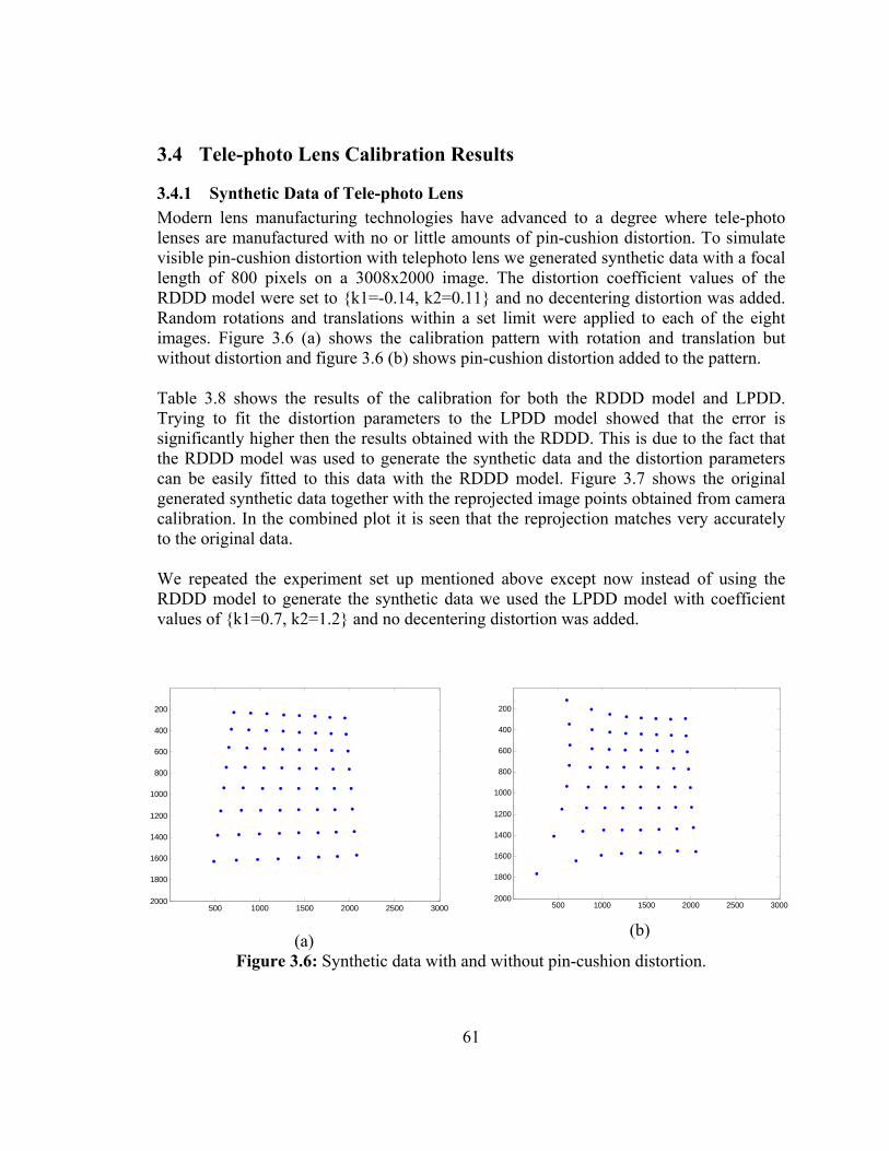
61

3.4 Tele-photo Lens Calibration Results

3.4.1 Synthetic Data of Tele-photo Lens Modern lens manufacturing technologies have advanced to a degree where tele-photo lenses are manufactured with no or little amounts of pin-cushion distortion. To simulate visible pin-cushion distortion with telephoto lens we generated synthetic data with a focal length of 800 pixels on a 3008x2000 image. The distortion coefficient values of the RDDD model were set to {k1=-0.14, k2=0.11} and no decentering distortion was added. Random rotations and translations within a set limit were applied to each of the eight images. Figure 3.6 (a) shows the calibration pattern with rotation and translation but without distortion and figure 3.6 (b) shows pin-cushion distortion added to the pattern. Table 3.8 shows the results of the calibration for both the RDDD model and LPDD. Trying to fit the distortion parameters to the LPDD model showed that the error is significantly higher then the results obtained with the RDDD. This is due to the fact that the RDDD model was used to generate the synthetic data and the distortion parameters can be easily fitted to this data with the RDDD model. Figure 3.7 shows the original generated synthetic data together with the reprojected image points obtained from camera calibration. In the combined plot it is seen that the reprojection matches very accurately to the original data. We repeated the experiment set up mentioned above except now instead of using the RDDD model to generate the synthetic data we used the LPDD model with coefficient values of {k1=0.7, k2=1.2} and no decentering distortion was added.

500 1000 1500 2000 2500 3000

200

400

600

800

1000

1200

1400

1600

1800

2000

(a)

500 1000 1500 2000 2500 3000

200

400

600

800

1000

1200

1400

1600

1800

2000

(b)

Figure 3.6: Synthetic data with and without pin-cushion distortion.

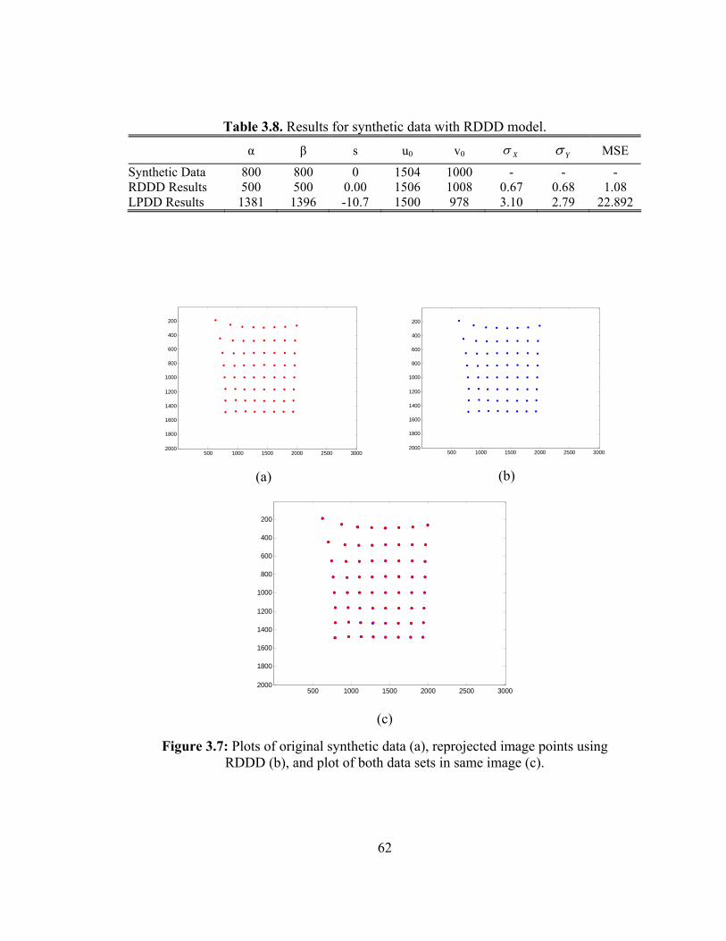
62

Table 3.8. Results for synthetic data with RDDD model.

α β s u0 v0 Xσ Yσ MSE

Synthetic Data 800 800 0 1504 1000 - - - RDDD Results 500 500 0.00 1506 1008 0.67 0.68 1.08 LPDD Results 1381 1396 -10.7 1500 978 3.10 2.79 22.892

500 1000 1500 2000 2500 3000

200

400

600

800

1000

1200

1400

1600

1800

2000

(a)

500 1000 1500 2000 2500 3000

200

400

600

800

1000

1200

1400

1600

1800

2000

(b)

500 1000 1500 2000 2500 3000

200

400

600

800

1000

1200

1400

1600

1800

2000

(c)

Figure 3.7: Plots of original synthetic data (a), reprojected image points using

RDDD (b), and plot of both data sets in same image (c).

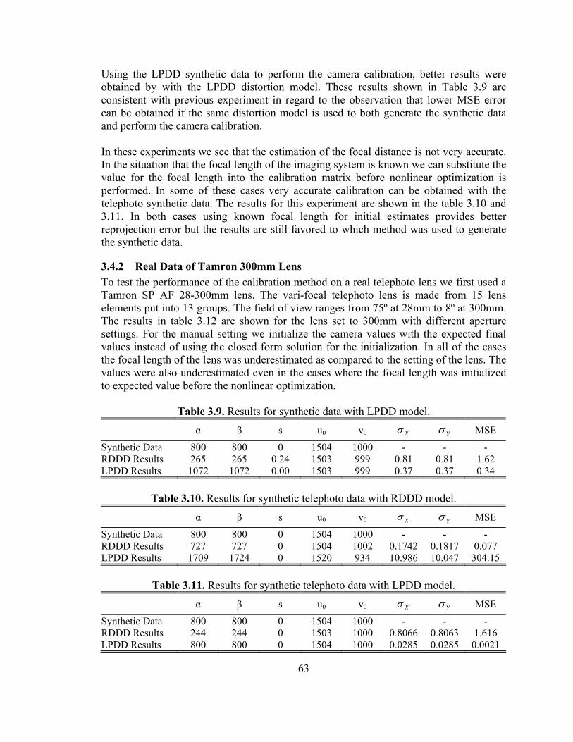
63

Using the LPDD synthetic data to perform the camera calibration, better results were obtained by with the LPDD distortion model. These results shown in Table 3.9 are consistent with previous experiment in regard to the observation that lower MSE error can be obtained if the same distortion model is used to both generate the synthetic data and perform the camera calibration. In these experiments we see that the estimation of the focal distance is not very accurate. In the situation that the focal length of the imaging system is known we can substitute the value for the focal length into the calibration matrix before nonlinear optimization is performed. In some of these cases very accurate calibration can be obtained with the telephoto synthetic data. The results for this experiment are shown in the table 3.10 and 3.11. In both cases using known focal length for initial estimates provides better reprojection error but the results are still favored to which method was used to generate the synthetic data.

3.4.2 Real Data of Tamron 300mm Lens To test the performance of the calibration method on a real telephoto lens we first used a Tamron SP AF 28-300mm lens. The vari-focal telephoto lens is made from 15 lens elements put into 13 groups. The field of view ranges from 75º at 28mm to 8º at 300mm. The results in table 3.12 are shown for the lens set to 300mm with different aperture settings. For the manual setting we initialize the camera values with the expected final values instead of using the closed form solution for the initialization. In all of the cases the focal length of the lens was underestimated as compared to the setting of the lens. The values were also underestimated even in the cases where the focal length was initialized to expected value before the nonlinear optimization.

Table 3.9. Results for synthetic data with LPDD model.

α β s u0 v0 Xσ Yσ MSE

Synthetic Data 800 800 0 1504 1000 - - - RDDD Results 265 265 0.24 1503 999 0.81 0.81 1.62 LPDD Results 1072 1072 0.00 1503 999 0.37 0.37 0.34

Table 3.10. Results for synthetic telephoto data with RDDD model.

α β s u0 v0 Xσ Yσ MSE

Synthetic Data 800 800 0 1504 1000 - - - RDDD Results 727 727 0 1504 1002 0.1742 0.1817 0.077 LPDD Results 1709 1724 0 1520 934 10.986 10.047 304.15

Table 3.11. Results for synthetic telephoto data with LPDD model.

α β s u0 v0 Xσ Yσ MSE

Synthetic Data 800 800 0 1504 1000 - - - RDDD Results 244 244 0 1503 1000 0.8066 0.8063 1.616 LPDD Results 800 800 0 1504 1000 0.0285 0.0285 0.0021

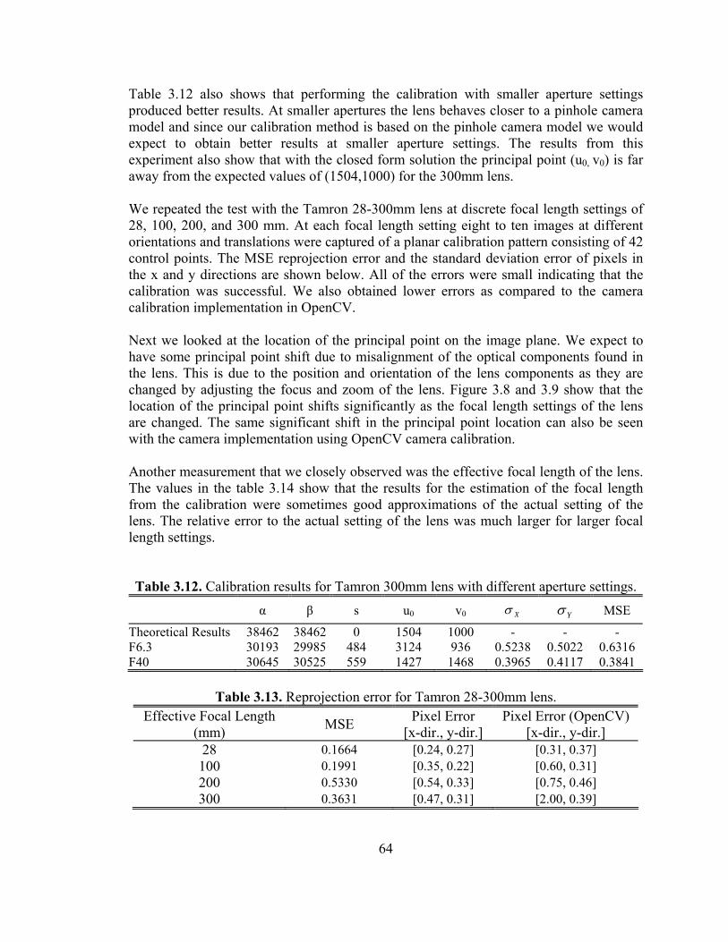
64

Table 3.12 also shows that performing the calibration with smaller aperture settings produced better results. At smaller apertures the lens behaves closer to a pinhole camera model and since our calibration method is based on the pinhole camera model we would expect to obtain better results at smaller aperture settings. The results from this experiment also show that with the closed form solution the principal point (u0, v0) is far away from the expected values of (1504,1000) for the 300mm lens. We repeated the test with the Tamron 28-300mm lens at discrete focal length settings of 28, 100, 200, and 300 mm. At each focal length setting eight to ten images at different orientations and translations were captured of a planar calibration pattern consisting of 42 control points. The MSE reprojection error and the standard deviation error of pixels in the x and y directions are shown below. All of the errors were small indicating that the calibration was successful. We also obtained lower errors as compared to the camera calibration implementation in OpenCV. Next we looked at the location of the principal point on the image plane. We expect to have some principal point shift due to misalignment of the optical components found in the lens. This is due to the position and orientation of the lens components as they are changed by adjusting the focus and zoom of the lens. Figure 3.8 and 3.9 show that the location of the principal point shifts significantly as the focal length settings of the lens are changed. The same significant shift in the principal point location can also be seen with the camera implementation using OpenCV camera calibration. Another measurement that we closely observed was the effective focal length of the lens. The values in the table 3.14 show that the results for the estimation of the focal length from the calibration were sometimes good approximations of the actual setting of the lens. The relative error to the actual setting of the lens was much larger for larger focal length settings. Table 3.12. Calibration results for Tamron 300mm lens with different aperture settings.

α β s u0 v0 Xσ Yσ MSE

Theoretical Results 38462 38462 0 1504 1000 - - - F6.3 30193 29985 484 3124 936 0.5238 0.5022 0.6316 F40 30645 30525 559 1427 1468 0.3965 0.4117 0.3841

Table 3.13. Reprojection error for Tamron 28-300mm lens. Effective Focal Length

(mm) MSE Pixel Error [x-dir., y-dir.]

Pixel Error (OpenCV) [x-dir., y-dir.]

28 0.1664 [0.24, 0.27] [0.31, 0.37] 100 0.1991 [0.35, 0.22] [0.60, 0.31] 200 0.5330 [0.54, 0.33] [0.75, 0.46] 300 0.3631 [0.47, 0.31] [2.00, 0.39]

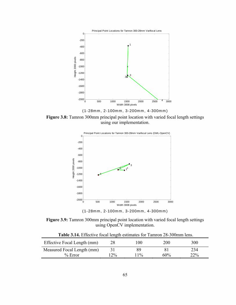
65

(1-28mm, 2-100mm, 3-200mm, 4-300mm)

Figure 3.8: Tamron 300mm principal point location with varied focal length settings using our implementation.

(1-28mm, 2-100mm, 3-200mm, 4-300mm)

Figure 3.9: Tamron 300mm principal point location with varied focal length settings using OpenCV implementation.

Table 3.14. Effective focal length estimates for Tamron 28-300mm lens.

Effective Focal Length (mm) 28 100 200 300 Measured Focal Length (mm) 31 89 81 234

% Error 12% 11% 60% 22%

0 500 1000 1500 2000 2500 3000-2000

-1800

-1600

-1400

-1200

-1000

-800

-600

-400

-200

0

Width 3008 pixels

Hei

ght 2

000

pixe

ls

Principal Point Locations for Tamron 300-28mm Varifocal Lens (GML-OpenCV)

123

4

x

0 500 1000 1500 2000 2500 3000-2000

-1800

-1600

-1400

-1200

-1000

-800

-600

-400

-200

0

Width 3008 pixels

Hei

ght 2

000

pixe

ls

Principal Point Locations for Tamron 300-28mm Varifocal Lens

1

23

4

x

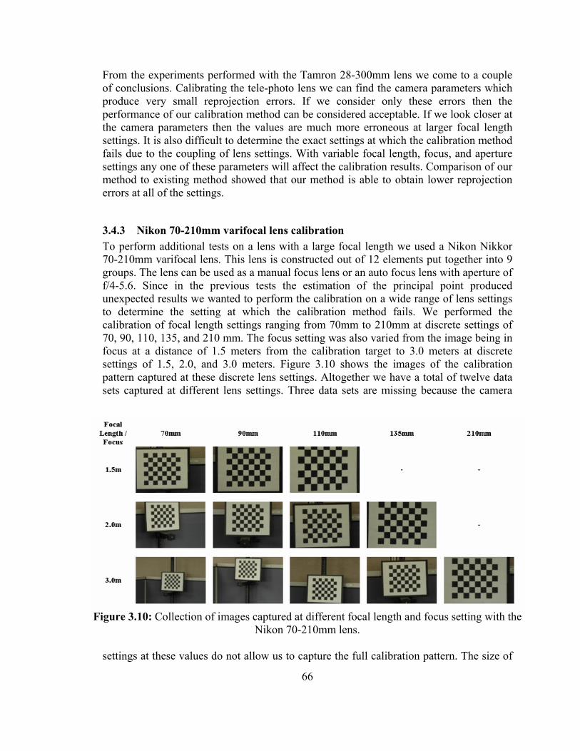
66

From the experiments performed with the Tamron 28-300mm lens we come to a couple of conclusions. Calibrating the tele-photo lens we can find the camera parameters which produce very small reprojection errors. If we consider only these errors then the performance of our calibration method can be considered acceptable. If we look closer at the camera parameters then the values are much more erroneous at larger focal length settings. It is also difficult to determine the exact settings at which the calibration method fails due to the coupling of lens settings. With variable focal length, focus, and aperture settings any one of these parameters will affect the calibration results. Comparison of our method to existing method showed that our method is able to obtain lower reprojection errors at all of the settings.

3.4.3 Nikon 70-210mm varifocal lens calibration To perform additional tests on a lens with a large focal length we used a Nikon Nikkor 70-210mm varifocal lens. This lens is constructed out of 12 elements put together into 9 groups. The lens can be used as a manual focus lens or an auto focus lens with aperture of f/4-5.6. Since in the previous tests the estimation of the principal point produced unexpected results we wanted to perform the calibration on a wide range of lens settings to determine the setting at which the calibration method fails. We performed the calibration of focal length settings ranging from 70mm to 210mm at discrete settings of 70, 90, 110, 135, and 210 mm. The focus setting was also varied from the image being in focus at a distance of 1.5 meters from the calibration target to 3.0 meters at discrete settings of 1.5, 2.0, and 3.0 meters. Figure 3.10 shows the images of the calibration pattern captured at these discrete lens settings. Altogether we have a total of twelve data sets captured at different lens settings. Three data sets are missing because the camera

settings at these values do not allow us to capture the full calibration pattern. The size of

Figure 3.10: Collection of images captured at different focal length and focus setting with the

Nikon 70-210mm lens.

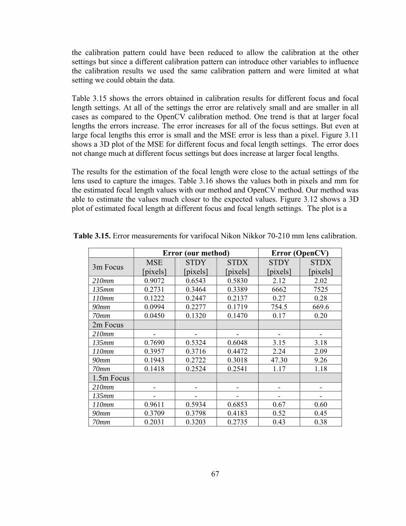
67

the calibration pattern could have been reduced to allow the calibration at the other settings but since a different calibration pattern can introduce other variables to influence the calibration results we used the same calibration pattern and were limited at what setting we could obtain the data. Table 3.15 shows the errors obtained in calibration results for different focus and focal length settings. At all of the settings the error are relatively small and are smaller in all cases as compared to the OpenCV calibration method. One trend is that at larger focal lengths the errors increase. The error increases for all of the focus settings. But even at large focal lengths this error is small and the MSE error is less than a pixel. Figure 3.11 shows a 3D plot of the MSE for different focus and focal length settings. The error does not change much at different focus settings but does increase at larger focal lengths. The results for the estimation of the focal length were close to the actual settings of the lens used to capture the images. Table 3.16 shows the values both in pixels and mm for the estimated focal length values with our method and OpenCV method. Our method was able to estimate the values much closer to the expected values. Figure 3.12 shows a 3D plot of estimated focal length at different focus and focal length settings. The plot is a Table 3.15. Error measurements for varifocal Nikon Nikkor 70-210 mm lens calibration.

Error (our method) Error (OpenCV)

3m Focus MSE [pixels]

STDY [pixels]

STDX [pixels]

STDY [pixels]

STDX [pixels]

210mm 0.9072 0.6543 0.5830 2.12 2.02 135mm 0.2731 0.3464 0.3389 6662 7525 110mm 0.1222 0.2447 0.2137 0.27 0.28 90mm 0.0994 0.2277 0.1719 754.5 669.6 70mm 0.0450 0.1320 0.1470 0.17 0.20 2m Focus 210mm - - - - - 135mm 0.7690 0.5324 0.6048 3.15 3.18 110mm 0.3957 0.3716 0.4472 2.24 2.09 90mm 0.1943 0.2722 0.3018 47.30 9.26 70mm 0.1418 0.2524 0.2541 1.17 1.18 1.5m Focus 210mm - - - - - 135mm - - - - - 110mm 0.9611 0.5934 0.6853 0.67 0.60 90mm 0.3709 0.3798 0.4183 0.52 0.45 70mm 0.2031 0.3203 0.2735 0.43 0.38

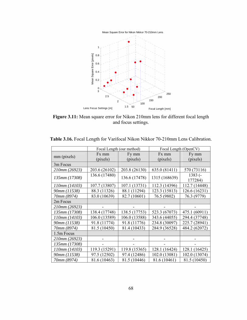
68

50100

150200

250

1.5

2

2.5

30

0.2

0.4

0.6

0.8

1

Focal Length [mm]

Mean Square Error for Nikon Nikkor 70-210mm Lens

Lens Focus Settings [m]

Mea

n S

quar

e E

rror [

pixe

ls]

Figure 3.11: Mean square error for Nikon 210mm lens for different focal length

and focus settings.

Table 3.16. Focal Length for Varifocal Nikon Nikkor 70-210mm Lens Calibration.

Focal Length (our method) Focal Length (OpenCV)

mm (pixels) Fx mm (pixels)

Fy mm (pixels)

Fx mm (pixels)

Fy mm (pixels)

3m Focus 210mm (26923) 203.6 (26102) 203.8 (26130) 635.0 (81411) 570 (73116)

135mm (17308) 136.6 (17480) 136.6 (17478) 1315 (168639) 1383 (-177284)

110mm (14103) 107.7 (13807) 107.1 (13731) 112.3 (14396) 112.7 (14448) 90mm (11538) 88.3 (11326) 88.1 (11294) 123.3 (15813) 126.6 (16231) 70mm (8974) 83.0 (10639) 82.7 (10601) 76.5 (9802) 76.3 (9779) 2m Focus 210mm (26923) - - - - 135mm (17308) 138.4 (17748) 138.5 (17753) 523.3 (67073) 475.1 (60911) 110mm (14103) 106.0 (13589) 106.0 (13588) 343.6 (44055) 294.4 (37748) 90mm (11538) 91.8 (11774) 91.8 (11776) 234.8 (30097) 225.7 (28941) 70mm (8974) 81.5 (10450) 81.4 (10433) 284.9 (36528) 484.2 (62072) 1.5m Focus 210mm (26923) - - - - 135mm (17308) - - - - 110mm (14103) 119.3 (15291) 119.8 (15365) 128.1 (16424) 128.1 (16425) 90mm (11538) 97.5 (12502) 97.4 (12486) 102.0 (13081) 102.0 (13074) 70mm (8974) 81.6 (10463) 81.5 (10446) 81.6 (10461) 81.5 (10450)

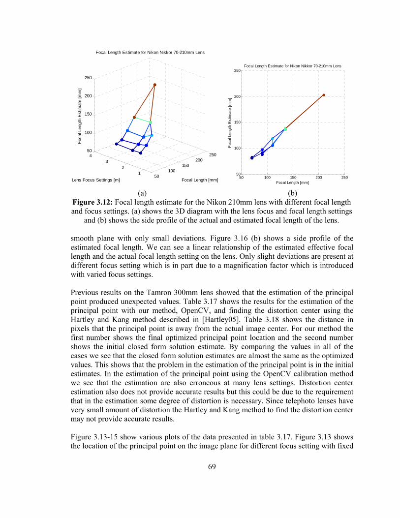
69

smooth plane with only small deviations. Figure 3.16 (b) shows a side profile of the estimated focal length. We can see a linear relationship of the estimated effective focal length and the actual focal length setting on the lens. Only slight deviations are present at different focus setting which is in part due to a magnification factor which is introduced with varied focus settings. Previous results on the Tamron 300mm lens showed that the estimation of the principal point produced unexpected values. Table 3.17 shows the results for the estimation of the principal point with our method, OpenCV, and finding the distortion center using the Hartley and Kang method described in [Hartley05]. Table 3.18 shows the distance in pixels that the principal point is away from the actual image center. For our method the first number shows the final optimized principal point location and the second number shows the initial closed form solution estimate. By comparing the values in all of the cases we see that the closed form solution estimates are almost the same as the optimized values. This shows that the problem in the estimation of the principal point is in the initial estimates. In the estimation of the principal point using the OpenCV calibration method we see that the estimation are also erroneous at many lens settings. Distortion center estimation also does not provide accurate results but this could be due to the requirement that in the estimation some degree of distortion is necessary. Since telephoto lenses have very small amount of distortion the Hartley and Kang method to find the distortion center may not provide accurate results. Figure 3.13-15 show various plots of the data presented in table 3.17. Figure 3.13 shows the location of the principal point on the image plane for different focus setting with fixed

50100

150200

250

12

34

50

100

150

200

250

Focal Length [mm]

Focal Length Estimate for Nikon Nikkor 70-210mm Lens

Lens Focus Settings [m]

Foca

l Len

gth

Est

imat

e [m

m]

50 100 150 200 25050

100

150

200

250

Focal Length [mm]

Focal Length Estimate for Nikon Nikkor 70-210mm Lens

Foca

l Len

gth

Est

imat

e [m

m]

(a) (b)

Figure 3.12: Focal length estimate for the Nikon 210mm lens with different focal length and focus settings. (a) shows the 3D diagram with the lens focus and focal length settings

and (b) shows the side profile of the actual and estimated focal length of the lens.

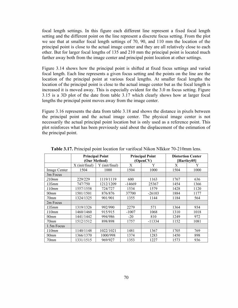
70

focal length settings. In this figure each different line represent a fixed focal length setting and the different point on the line represent a discrete focus setting. From the plot we see that at smaller focal length settings of 70, 90, and 110 mm the location of the principal point is close to the actual image center and they are all relatively close to each other. But for larger focal lengths of 135 and 210 mm the principal point is located much farther away both from the image center and principal point location at other settings. Figure 3.14 shows how the principal point is shifted at fixed focus settings and varied focal length. Each line represents a given focus setting and the points on the line are the location of the principal point at various focal lengths. At smaller focal lengths the location of the principal point is close to the actual image center but as the focal length is increased it is moved away. This is especially evident for the 3.0 m focus setting. Figure 3.15 is a 3D plot of the date from table 3.17 which clearly shows how at larger focal lengths the principal point moves away from the image center. Figure 3.16 represents the data from table 3.18 and shows the distance in pixels between the principal point and the actual image center. The physical image center is not necessarily the actual principal point location but is only used as a reference point. This plot reinforces what has been previously said about the displacement of the estimation of the principal point.

Table 3.17. Principal point location for varifocal Nikon NIkkor 70-210mm lens.

Principal Point (Our Method)

Principal Point (OpenCV)

Distortion Center [Hartley05]

X (init/final) Y (init/final) X Y X Y Image Center 1504 1000 1504 1000 1504 1000 3m Focus 210mm 229/229 1119/1119 600 1163 1767 636 135mm 747/750 1212/1209 -14669 25367 1454 1366 110mm 1557/1558 724/727 1534 1579 1428 1120 90mm 1501/1501 876/876 37700 -26103 1884 1177 70mm 1324/1325 901/901 1355 1144 1184 564 2m Focus 135mm 1319/1326 992/990 2279 571 1364 934 110mm 1460/1460 915/915 -1007 1068 1310 1018 90mm 1441/1442 994/986 -20 810 1249 972 70mm 1512/1512 898/898 1757 -11334 1152 1081 1.5m Focus 110mm 1140/1148 1022/1021 1481 1367 1705 769 90mm 1366/1370 1000/998 1374 1283 1450 898 70mm 1331/1515 969/927 1353 1227 1573 936

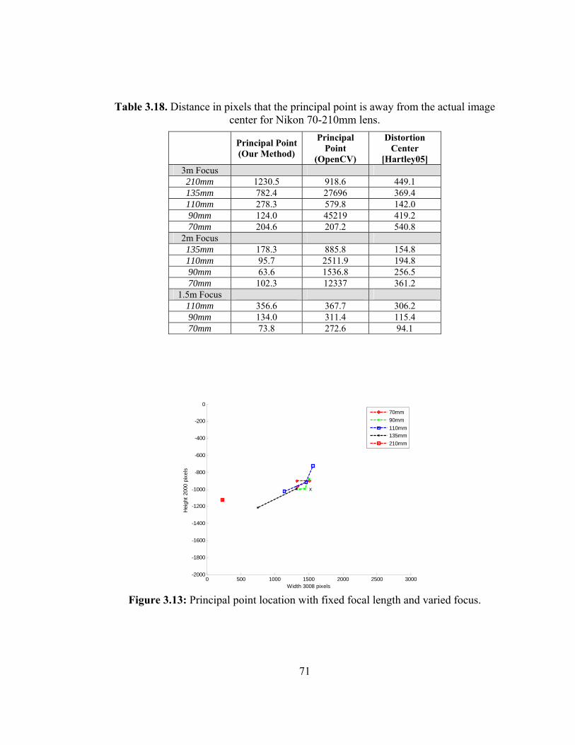
71

Table 3.18. Distance in pixels that the principal point is away from the actual image center for Nikon 70-210mm lens.

Principal Point (Our Method)

Principal Point

(OpenCV)

Distortion Center

[Hartley05] 3m Focus 210mm 1230.5 918.6 449.1 135mm 782.4 27696 369.4 110mm 278.3 579.8 142.0 90mm 124.0 45219 419.2 70mm 204.6 207.2 540.8

2m Focus 135mm 178.3 885.8 154.8 110mm 95.7 2511.9 194.8 90mm 63.6 1536.8 256.5 70mm 102.3 12337 361.2

1.5m Focus 110mm 356.6 367.7 306.2 90mm 134.0 311.4 115.4 70mm 73.8 272.6 94.1

0 500 1000 1500 2000 2500 3000-2000

-1800

-1600

-1400

-1200

-1000

-800

-600

-400

-200

0

Width 3008 pixels

Hei

ght 2

000

pixe

ls

x

70mm90mm110mm135mm210mm

Figure 3.13: Principal point location with fixed focal length and varied focus.

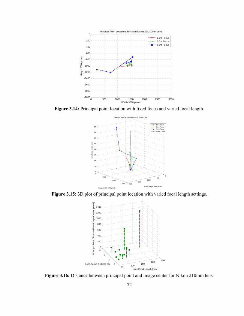
72

0 500 1000 1500 2000 2500 3000-2000

-1800

-1600

-1400

-1200

-1000

-800

-600

-400

-200

0

Width 3008 pixels

Hei

ght 2

000

pixe

ls

Principal Point Locations for Nikon Nikkor 70-210mm Lens

1x

1.5m Focus2.0m Focus3.0m Focus

Figure 3.14: Principal point location with fixed focus and varied focal length.

0

1000

2000

3000 -2000-1500

-1000-500

0

60

80

100

120

140

160

180

200

220

Image Height 2000 pixels

Principal Point for Nikon Nikkor 70-210mm Lens

Image Width 3008 pixels

Lens

Foc

al L

engt

h [m

m]

1.5m Focus2.0m Focus3.0m FocusImage Center

Figure 3.15: 3D plot of principal point location with varied focal length settings.

50100

150200

250

1

2

3

40

200

400

600

800

1000

1200

1400

Lens Focal Length [mm]

Lens Focus Settings [m]

Prin

cipa

l Poi

nt D

ista

nce

From

Imag

e C

ente

r [pi

xels

]

Figure 3.16: Distance between principal point and image center for Nikon 210mm lens.

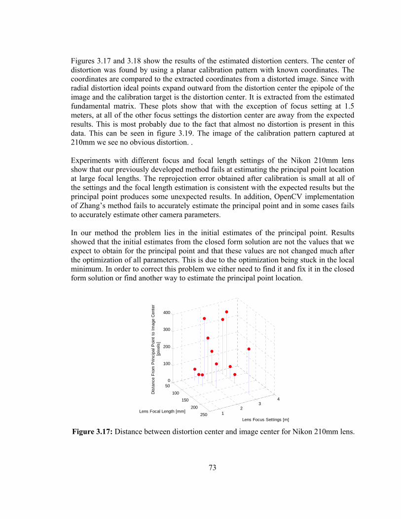
73

Figures 3.17 and 3.18 show the results of the estimated distortion centers. The center of distortion was found by using a planar calibration pattern with known coordinates. The coordinates are compared to the extracted coordinates from a distorted image. Since with radial distortion ideal points expand outward from the distortion center the epipole of the image and the calibration target is the distortion center. It is extracted from the estimated fundamental matrix. These plots show that with the exception of focus setting at 1.5 meters, at all of the other focus settings the distortion center are away from the expected results. This is most probably due to the fact that almost no distortion is present in this data. This can be seen in figure 3.19. The image of the calibration pattern captured at 210mm we see no obvious distortion. . Experiments with different focus and focal length settings of the Nikon 210mm lens show that our previously developed method fails at estimating the principal point location at large focal lengths. The reprojection error obtained after calibration is small at all of the settings and the focal length estimation is consistent with the expected results but the principal point produces some unexpected results. In addition, OpenCV implementation of Zhang’s method fails to accurately estimate the principal point and in some cases fails to accurately estimate other camera parameters. In our method the problem lies in the initial estimates of the principal point. Results showed that the initial estimates from the closed form solution are not the values that we expect to obtain for the principal point and that these values are not changed much after the optimization of all parameters. This is due to the optimization being stuck in the local minimum. In order to correct this problem we either need to find it and fix it in the closed form solution or find another way to estimate the principal point location.

50

100150

200

250 12

34

0

100

200

300

400

Lens Focus Settings [m]

Lens Focal Length [mm]

Dis

tanc

e Fr

om P

rinci

pal P

oint

to Im

age

Cen

ter

[pix

els]

Figure 3.17: Distance between distortion center and image center for Nikon 210mm lens.

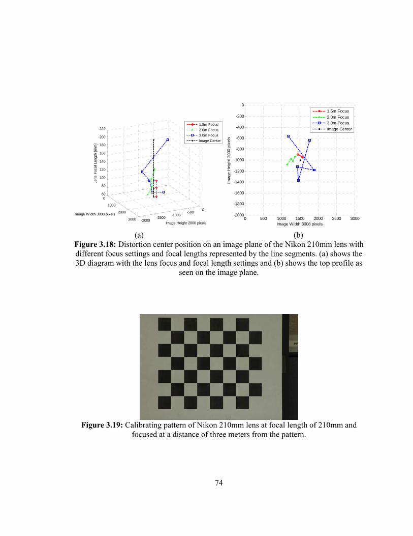
74

0

1000

2000

3000 -2000-1500

-1000-500

0

60

80

100

120

140

160

180

200

220

Image Height 2000 pixels

Image Width 3008 pixels

Lens

Foc

al L

engt

h [m

m]

1.5m Focus2.0m Focus3.0m FocusImage Center

0 500 1000 1500 2000 2500 3000-2000

-1800

-1600

-1400

-1200

-1000

-800

-600

-400

-200

0

Image Width 3008 pixels

Imag

e H

eigh

t 200

0 pi

xels

1.5m Focus2.0m Focus3.0m FocusImage Center

(a) (b)

Figure 3.18: Distortion center position on an image plane of the Nikon 210mm lens with different focus settings and focal lengths represented by the line segments. (a) shows the 3D diagram with the lens focus and focal length settings and (b) shows the top profile as

seen on the image plane.

Figure 3.19: Calibrating pattern of Nikon 210mm lens at focal length of 210mm and

focused at a distance of three meters from the pattern.

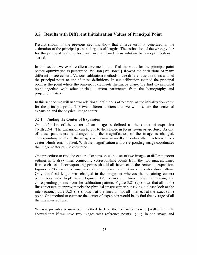
75

3.5 Results with Different Initialization Values of Principal Point Results shown in the previous sections show that a large error is generated in the estimation of the principal point at large focal lengths. The estimation of the wrong value for the principal point is first seen in the closed form solution before optimization is started. In this section we explore alternative methods to find the value for the principal point before optimization is performed. Willson [Willson93] showed the definitions of many different image centers. Various calibration methods make different assumptions and set the principal point to one of these definitions. In our calibration method the principal point is the point where the principal axis meets the image plane. We find the principal point together with other intrinsic camera parameters from the homography and projection matrix. In this section we will use two additional definitions of “center” as the initialization value for the principal point. The two different centers that we will use are the center of expansion and the physical image center.

3.5.1 Finding the Center of Expansion One definition of the center of an image is defined as the center of expansion [Willson94]. The expansion can be due to the change in focus, zoom or aperture. As one of these parameters is changed and the magnification of the image is changed, corresponding points in the images will move inwardly or outwardly in reference to a center which remains fixed. With the magnification and corresponding image coordinates the image center can be estimated. One procedure to find the center of expansion with a set of two images at different zoom settings is to draw lines connecting corresponding points from the two images. Lines from each set of corresponding points should all intersect at the center of expansion. Figures 3.20 shows two images captured at 50mm and 70mm of a calibration pattern. Only the focal length was changed in the image set whereas the remaining camera parameters were kept fixed. Figures 3.21 shows the lines drawn connecting the corresponding points from the calibration pattern. Figure 3.21 (a) shows that all of the lines intersect at approximately the physical image center but taking a closer look at the intersection, figure 3.21 (b), shows that the lines do not all intersect at the exact same point. One method to estimate the center of expansion would be to find the average of all the line intersections. Willson provides a numerical method to find the expansion center [Willson93]. He showed that if we have two images with reference points nPP ...1 in one image and

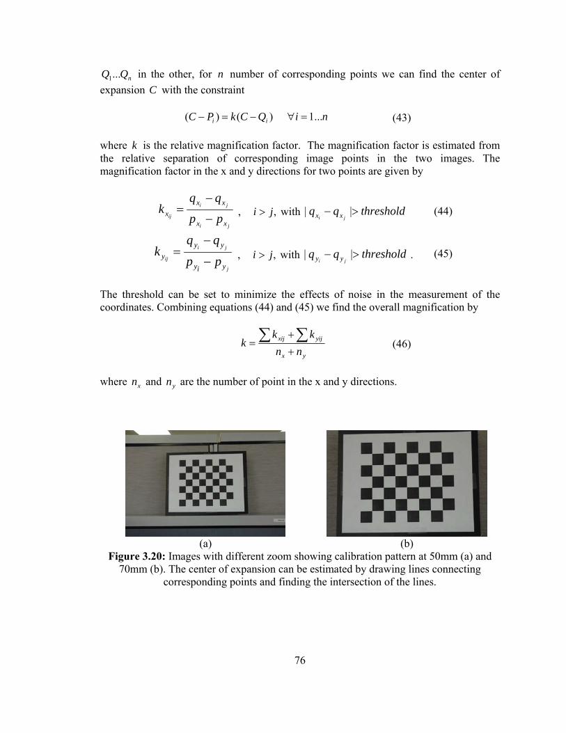
76

nQQ ...1 in the other, for n number of corresponding points we can find the center of expansion C with the constraint

)()( ii QCkPC −=− ni ...1=∀ (43) where k is the relative magnification factor. The magnification factor is estimated from the relative separation of corresponding image points in the two images. The magnification factor in the x and y directions for two points are given by

ji

ji

ijxx

xxx pp

qqk

−

−= , ,ji > with thresholdqq

ji xx >− || (44)

j

ji

ijyiy

yyy pp

qqk

−

−= , ,ji > with thresholdqq

ji yy >− || . (45)

The threshold can be set to minimize the effects of noise in the measurement of the coordinates. Combining equations (44) and (45) we find the overall magnification by

yx

yijxij

nnkk

k+

+= ∑ ∑ (46)

where xn and yn are the number of point in the x and y directions.

(a)

(b)

Figure 3.20: Images with different zoom showing calibration pattern at 50mm (a) and 70mm (b). The center of expansion can be estimated by drawing lines connecting

corresponding points and finding the intersection of the lines.

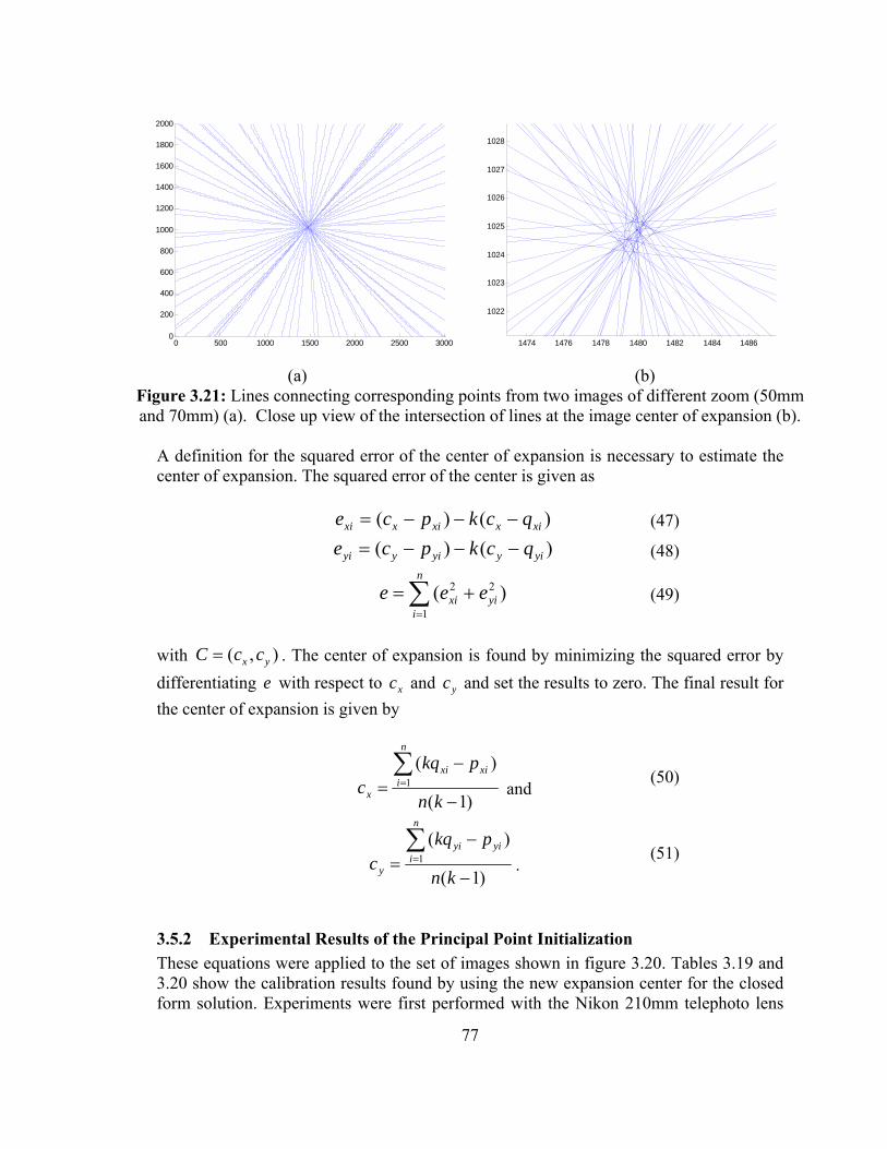
77

0 500 1000 1500 2000 2500 30000

200

400

600

800

1000

1200

1400

1600

1800

2000

(a)

1474 1476 1478 1480 1482 1484 1486

1022

1023

1024

1025

1026

1027

1028

(b)

Figure 3.21: Lines connecting corresponding points from two images of different zoom (50mm and 70mm) (a). Close up view of the intersection of lines at the image center of expansion (b).

A definition for the squared error of the center of expansion is necessary to estimate the center of expansion. The squared error of the center is given as

)()( xixxixxi qckpce −−−= (47) )()( yiyyiyyi qckpce −−−= (48)

∑=

+=n

iyixi eee

1

22 )( (49)

with ( , )x yC c c= . The center of expansion is found by minimizing the squared error by differentiating e with respect to xc and yc and set the results to zero. The final result for the center of expansion is given by

)1(

)(1

−

−=∑=

kn

pkqc

n

ixixi

x and (50)

)1(

)(1

−

−=∑=

kn

pkqc

n

iyiyi

y . (51)

3.5.2 Experimental Results of the Principal Point Initialization These equations were applied to the set of images shown in figure 3.20. Tables 3.19 and 3.20 show the calibration results found by using the new expansion center for the closed form solution. Experiments were first performed with the Nikon 210mm telephoto lens

78

set at focal length of 210mm. In the calibration experiments we varied the values of principal point before nonlinear optimization. In one experiment we set the principal point to the numerical image center (1504, 1000). We also tried to set the initial principal point value to the center of expansion which was found by the method described in the previous section (1481.7, 1019.2). All of the results are compared to the results obtained by performing normal calibration with the initial value of the principal point extracted from the closed form solution. Eight images with resolution of 3008 x 2000 were captured of a planar calibration pattern with 42 control points. Table 3.19 shows the results for three different scenarios using the LPDD distortion model. For the normal case the closed form solution of the principal point location was used as the initialization value for the nonlinear optimization. The MSE reprojection error obtained is smaller than a pixel but the location of the principal point is about 1280 pixels away from the actual image center. The results we obtained using the actual image center as the initialization value for the principal point produced a MSE reprojection error of only 0.4446 pixels. This error is about half as much as the error with the unaltered calibration method. Similar reprojection error was also obtained using the expansion center as the initialization for the principal point. Results with the image center and the expansion center initializations also produced the expected values for the optimized principal point location. From these experiments we see that using other meaningful definitions of the principal point can also produce low reprojection errors. This altered method provides much better reprojection error while also providing good estimates of all the camera parameters such as the focal length of the camera. Table 3.20 shows the same experiments performed with the RDDD model. Observations made with the LPDD model are also true with the RDDD distortion model. ___

Table 3.19. Calibration results with varied initialization values for principal point with LPDD model.

α β s u0 v0 1κ 2κ MSE No Initilization 26105.9 26118.4 -55.7 229.3 1119.5 1.0006 0.4871 0.8828 Image Center 26174.1 26150.3 46.1 1503.1 999.0 1.0000 2.6939 0.4446 Expansion Center 26162.8 26140.3 45.1 1481.6 1022.3 1.0005 2.6948 0.4437

Table 3.20. Calibration results with varied initialization values for principal point with

RDDD model. α β s u0 v0 1κ 2κ MSE

No Initilization 26118.6 26123.2 -36.2 229.1 1119.4 -0.6273 67.381 0.6917

Image Center 26146.3 26123.2 47.3 1504.4 999.5 3.0245 -231.44 0.4422 Expansion Center 26139.8 26117.5 44.7 1482.2 1022.8 2.8807 -178.95 0.4426

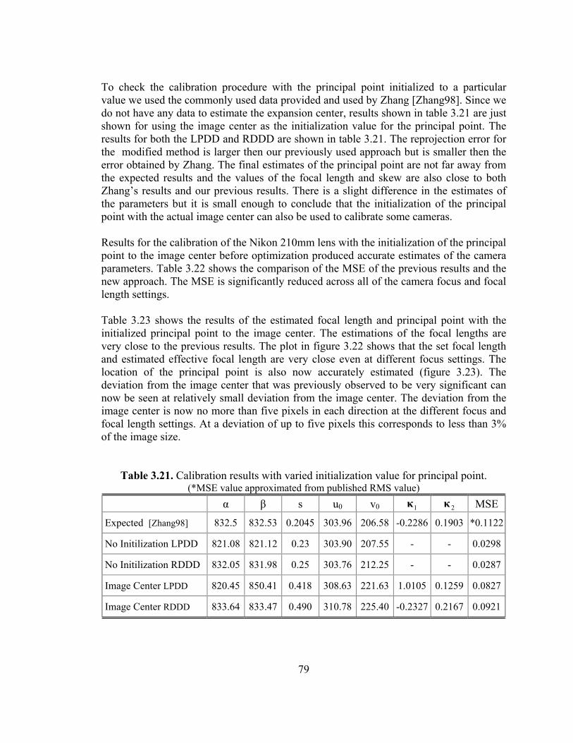
79

To check the calibration procedure with the principal point initialized to a particular value we used the commonly used data provided and used by Zhang [Zhang98]. Since we do not have any data to estimate the expansion center, results shown in table 3.21 are just shown for using the image center as the initialization value for the principal point. The results for both the LPDD and RDDD are shown in table 3.21. The reprojection error for the modified method is larger then our previously used approach but is smaller then the error obtained by Zhang. The final estimates of the principal point are not far away from the expected results and the values of the focal length and skew are also close to both Zhang’s results and our previous results. There is a slight difference in the estimates of the parameters but it is small enough to conclude that the initialization of the principal point with the actual image center can also be used to calibrate some cameras. Results for the calibration of the Nikon 210mm lens with the initialization of the principal point to the image center before optimization produced accurate estimates of the camera parameters. Table 3.22 shows the comparison of the MSE of the previous results and the new approach. The MSE is significantly reduced across all of the camera focus and focal length settings. Table 3.23 shows the results of the estimated focal length and principal point with the initialized principal point to the image center. The estimations of the focal lengths are very close to the previous results. The plot in figure 3.22 shows that the set focal length and estimated effective focal length are very close even at different focus settings. The location of the principal point is also now accurately estimated (figure 3.23). The deviation from the image center that was previously observed to be very significant can now be seen at relatively small deviation from the image center. The deviation from the image center is now no more than five pixels in each direction at the different focus and focal length settings. At a deviation of up to five pixels this corresponds to less than 3% of the image size.

Table 3.21. Calibration results with varied initialization value for principal point. (*MSE value approximated from published RMS value)

α β s u0 v0 1κ 2κ MSE

Expected [Zhang98] 832.5 832.53 0.2045 303.96 206.58 -0.2286 0.1903 *0.1122

No Initilization LPDD 821.08 821.12 0.23 303.90 207.55 - - 0.0298

No Initilization RDDD 832.05 831.98 0.25 303.76 212.25 - - 0.0287

Image Center LPDD 820.45 850.41 0.418 308.63 221.63 1.0105 0.1259 0.0827

Image Center RDDD 833.64 833.47 0.490 310.78 225.40 -0.2327 0.2167 0.0921

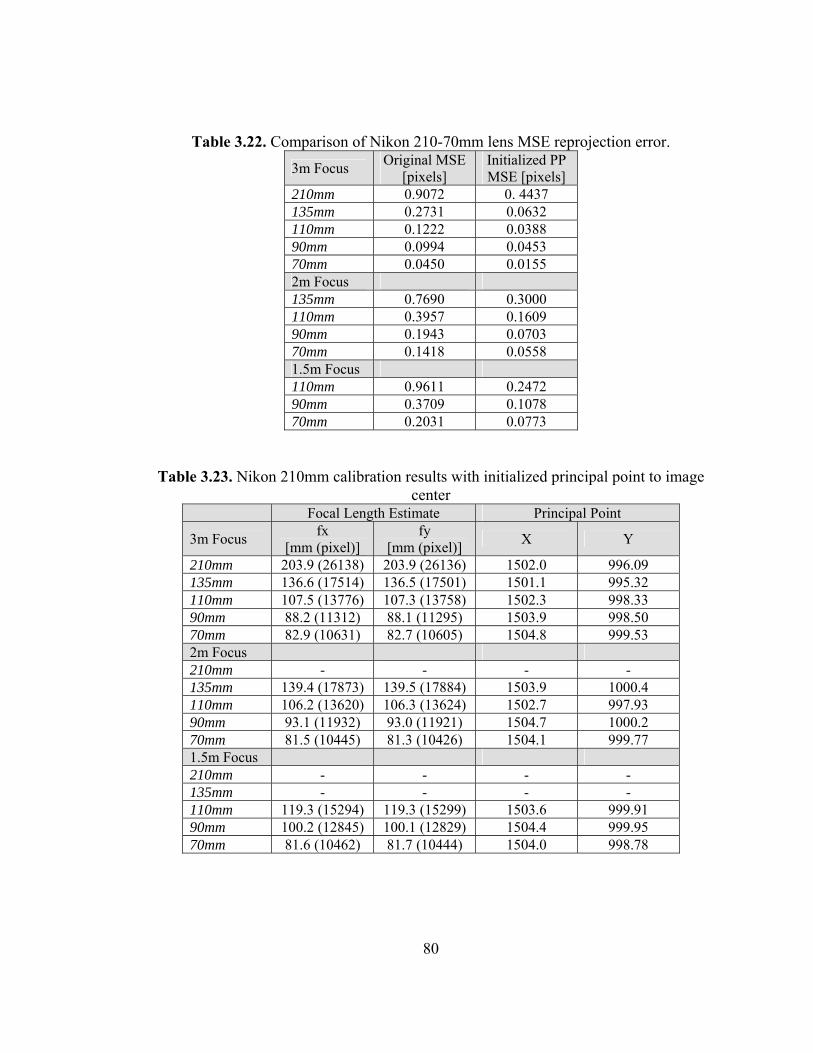
80

Table 3.22. Comparison of Nikon 210-70mm lens MSE reprojection error. 3m Focus Original MSE

[pixels] Initialized PP MSE [pixels]

210mm 0.9072 0. 4437 135mm 0.2731 0.0632 110mm 0.1222 0.0388 90mm 0.0994 0.0453 70mm 0.0450 0.0155 2m Focus 135mm 0.7690 0.3000 110mm 0.3957 0.1609 90mm 0.1943 0.0703 70mm 0.1418 0.0558 1.5m Focus 110mm 0.9611 0.2472 90mm 0.3709 0.1078 70mm 0.2031 0.0773

Table 3.23. Nikon 210mm calibration results with initialized principal point to image center

Focal Length Estimate Principal Point

3m Focus fx [mm (pixel)]

fy [mm (pixel)] X Y

210mm 203.9 (26138) 203.9 (26136) 1502.0 996.09 135mm 136.6 (17514) 136.5 (17501) 1501.1 995.32 110mm 107.5 (13776) 107.3 (13758) 1502.3 998.33 90mm 88.2 (11312) 88.1 (11295) 1503.9 998.50 70mm 82.9 (10631) 82.7 (10605) 1504.8 999.53 2m Focus 210mm - - - - 135mm 139.4 (17873) 139.5 (17884) 1503.9 1000.4 110mm 106.2 (13620) 106.3 (13624) 1502.7 997.93 90mm 93.1 (11932) 93.0 (11921) 1504.7 1000.2 70mm 81.5 (10445) 81.3 (10426) 1504.1 999.77 1.5m Focus 210mm - - - - 135mm - - - - 110mm 119.3 (15294) 119.3 (15299) 1503.6 999.91 90mm 100.2 (12845) 100.1 (12829) 1504.4 999.95 70mm 81.6 (10462) 81.7 (10444) 1504.0 998.78

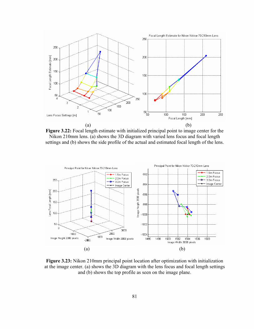
81

(a) (b)

Figure 3.22: Focal length estimate with initialized principal point to image center for the Nikon 210mm lens. (a) shows the 3D diagram with varied lens focus and focal length

settings and (b) shows the side profile of the actual and estimated focal length of the lens.

(a) (b)

Figure 3.23: Nikon 210mm principal point location after optimization with initialization at the image center. (a) shows the 3D diagram with the lens focus and focal length settings

and (b) shows the top profile as seen on the image plane.

82

In this section we have shown that we can use other definitions of image center as the initialization values for the principal point. Since at large focal lengths the closed form solution fails to provide good estimates of the principal point, the center of expansion or the actual image center can provide better principal point initialization. We have shown that with the telephoto lens much better results and lower reprojection errors are obtained with the new approach. Using Zhang’s data [Zhang98] of a regular lens with little distortion we can also obtain good estimates of all the parameters with the initialization of principal point set to the image center. From these experiments we can conclude that for large focal length settings it is possible to use the zoom of expansion or actual image center for the initialization value of the principal point before nonlinear optimization and achieve good calibration results using our approach.

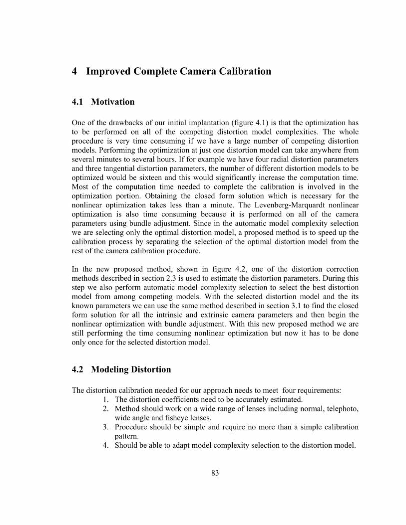
83

4 Improved Complete Camera Calibration

4.1 Motivation One of the drawbacks of our initial implantation (figure 4.1) is that the optimization has to be performed on all of the competing distortion model complexities. The whole procedure is very time consuming if we have a large number of competing distortion models. Performing the optimization at just one distortion model can take anywhere from several minutes to several hours. If for example we have four radial distortion parameters and three tangential distortion parameters, the number of different distortion models to be optimized would be sixteen and this would significantly increase the computation time. Most of the computation time needed to complete the calibration is involved in the optimization portion. Obtaining the closed form solution which is necessary for the nonlinear optimization takes less than a minute. The Levenberg-Marquardt nonlinear optimization is also time consuming because it is performed on all of the camera parameters using bundle adjustment. Since in the automatic model complexity selection we are selecting only the optimal distortion model, a proposed method is to speed up the calibration process by separating the selection of the optimal distortion model from the rest of the camera calibration procedure. In the new proposed method, shown in figure 4.2, one of the distortion correction methods described in section 2.3 is used to estimate the distortion parameters. During this step we also perform automatic model complexity selection to select the best distortion model from among competing models. With the selected distortion model and the its known parameters we can use the same method described in section 3.1 to find the closed form solution for all the intrinsic and extrinsic camera parameters and then begin the nonlinear optimization with bundle adjustment. With this new proposed method we are still performing the time consuming nonlinear optimization but now it has to be done only once for the selected distortion model.

4.2 Modeling Distortion The distortion calibration needed for our approach needs to meet four requirements:

1. The distortion coefficients need to be accurately estimated. 2. Method should work on a wide range of lenses including normal, telephoto,

wide angle and fisheye lenses. 3. Procedure should be simple and require no more than a simple calibration

pattern. 4. Should be able to adapt model complexity selection to the distortion model.

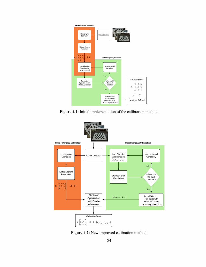
84

Corner DetectionHomography Estimation

Extract Camera Parameters

Lens Distortion Approximation

Parameter Optimization with

Bundle Adjustment

Initial Parameter Estimation

Model Complexity Selection

Is the model the most

Complex?

Increase Model Complexity

Model SelectionPick model with lowest AIC score

⎟⎟⎟

⎠

⎞

⎜⎜⎜

⎝

⎛=

1000 0

0

vus

βα

K

( ),...,,...,, 21,21 ttκκ

TR

No

Yes

Calibration Results

⎟⎟⎟

⎠

⎞

⎜⎜⎜

⎝

⎛=

1000 0

0

vus

βα

K

R T

( ),...,,...,, 21,21 ttκκ( ) kL i 2;log2AIC +−= mθ

Figure 4.1: Initial implementation of the calibration method.

Corner DetectionHomography Estimation

Extract Camera Parameters

Lens Distortion Approximation

Distortion Error Calculations

Initial Parameter Estimation Model Complexity Selection

Is the model the most

Complex?

Increase Model Complexity

Model SelectionPick model with lowest AIC score

⎟⎟⎟

⎠

⎞

⎜⎜⎜

⎝

⎛=

1000 0

0

vus

βα

K

( ),...,,...,, 21,21 ttκκ

TR

No

Yes

Nonlinear Optimization with Bundle Adjustment

Calibration Results

⎟⎟⎟

⎠

⎞

⎜⎜⎜

⎝

⎛=

1000 0

0

vus

βα

K R T ( ),...,,...,, 21,21 ttκκ

( ),...,,...,, 21,21 ttκκ

( ) kL i 2;log2AIC +−= mθ

Figure 4.2: New improved calibration method.

85

As will be shown later each one of these requirements can be achieved by expanding on the initial implementation. In the new camera calibration method the distortion needs to be accurately modeled before the nonlinear optimization of all the camera parameters. The distortion must be modeled accurately because we will be selecting the distortion model before other parameters are accurately estimated. In the event that the distortion is not accurately approximated the model selection may not pick the optimal distortion model from the competing model. This is shown with the FUJINON 1.4-3.1 mm lens on IQEye3 camera with the wide angle setting using the RDDD model (Table 4.1) and LPDD model (Table 4.2). The experiment was performed using the closed form solution to select the distortion model instead waiting to perform the optimization of the camera parameters. Using the previous calibration method, if model complexity selection is performed before optimizing the distortion coefficients then the selected model is more complex than after the optimization of the coefficients. The second requirement is that the distortion calibration method should work on a wide range of camera lenses. We are still interested in a complete camera calibration method which can work on a wide range of systems and as a result, should be able to model distortion regardless of its complexity. The third and fourth requirements extend from the original calibration method. We want to keep the calibration method simple. In the original method a simple planar checkerboard calibration pattern was used to perform the calibration and it was a relatively simple procedure. We will continue to use this pattern for the distortion calibration. Since we are interested in performing distortion model complexity selection we need a distortion calibration method on which we can apply the information theoretic criterion (AIC) [Akaike74]. Some methods, due to various assumptions and specific applications, use a fixed distortion model to approximate the distortion [Fitzgiboon01]. Others present methods to fix the distortion by using a nonparametric model [Stevenson96]. We will concentrate on distortion models which can incorporate the radial polynomial model and the lens projection polynomial model.

Table 4.1. RDDD model selection for wide angle lens with and without optimization.

MDL BIC SSD CAIC p q p q p q p q Optimized Coefficients 2 2 2 0 2 0 2 0 Closed Form Solution 3 0 3 0 3 0 3 0

Table 4.2. LPDD model selection for wide angle lens with and without optimization. MDL BIC SSD CAIC p q p q p q p q

Optimized Coefficients 1 0 1 2 1 2 1 0 Closed Form Solution 4 0 4 0 4 0 4 0

86

A survey of distortion calibration methods revealed two groups of methods which may be able to satisfy all of the requirements. The first group relies on the fact that straight lines have to be straight [Ahmed05, Borreto03, Brauer-Burchardt01, Devenrnay01, Swaminathan01, Xu06]. The second group relies on having point correspondence from several images to estimate the distortion [Hartely05, Li05, Stein97, Thirthala05]. Some of these methods require the use of a calibration pattern while other present procedures which only require the presence of particular image features to perform the calibration. Since we are using the calibration pattern for the closed form estimation of other camera parameters we will also use the calibration pattern in the distortion calibration.

4.3 Optimizing Distortion Only One proposed method is to alter the originally developed calibration method. In the original method instead of optimizing all of the parameters in the nonlinear optimization step we optimize only the distortion parameters. The optimization of only the distortion parameters is performed for all of the competing distortion models and then using our model selection criteria we select the optimum distortion model. We then repeat the complete calibration with the selected distortion model and using bundle adjustment alternate between optimizing distortion parameters and the other camera parameters. The advantage of this method is that instead of optimizing all of the parameters we are only optimizing the radial and tangential coefficients for all of the competing distortion models. The model selection takes up anywhere from five to ten minutes as compared to several hours by using the original method. Tables 4.3 and 4.4 show the automatic distortion model selection results for LPDD and RDDD using real data. Comparing these results to the original results we can make the observation that in few cases the selected distortion complexities match but in most cases the selected complexities of the distortion models are higher. The reason for the difference in the selected distortion model is that without optimizing the camera parameters from the closed form solution the reprojection errors are higher. The MSE measurements (Table 4.5 and Table 4.6) with only the optimized distortion coefficients are not an accurate representation of how the model will perform after all of the camera parameters are optimized. This approach to find the complexity of the necessary distortion model does not provide accurate results because we use a closed form solution to the linear terms (ex. Camera matrix, rotation matrix) to optimize the nonlinear distortion terms. During the optimization the distortion parameters are optimized using the reprojection error which is dependent on the closed form solution. As a result the selected distortion model from the optimized distortion coefficients is not the optimal model. In order to accurately select the distortion model from competing models we need an error measure which does not require good estimates of other camera parameters.

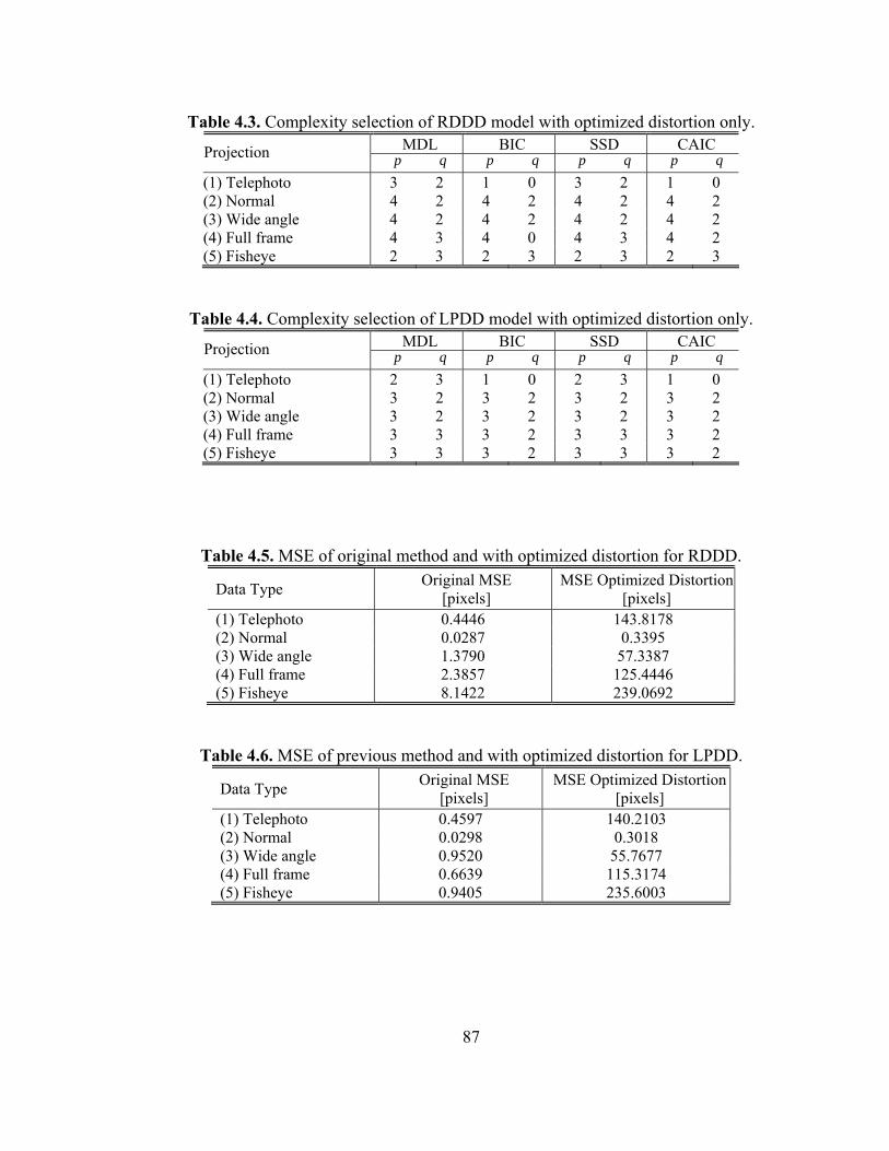
87

Table 4.3. Complexity selection of RDDD model with optimized distortion only.

MDL BIC SSD CAIC Projection p q p q p q p q (1) Telephoto 3 2 1 0 3 2 1 0 (2) Normal 4 2 4 2 4 2 4 2 (3) Wide angle 4 2 4 2 4 2 4 2 (4) Full frame 4 3 4 0 4 3 4 2 (5) Fisheye 2 3 2 3 2 3 2 3

Table 4.4. Complexity selection of LPDD model with optimized distortion only. MDL BIC SSD CAIC Projection p q p q p q p q

(1) Telephoto 2 3 1 0 2 3 1 0 (2) Normal 3 2 3 2 3 2 3 2 (3) Wide angle 3 2 3 2 3 2 3 2 (4) Full frame 3 3 3 2 3 3 3 2 (5) Fisheye 3 3 3 2 3 3 3 2

Table 4.5. MSE of original method and with optimized distortion for RDDD.

Data Type Original MSE [pixels]

MSE Optimized Distortion[pixels]

(1) Telephoto 0.4446 143.8178 (2) Normal 0.0287 0.3395 (3) Wide angle 1.3790 57.3387 (4) Full frame 2.3857 125.4446 (5) Fisheye 8.1422 239.0692

Table 4.6. MSE of previous method and with optimized distortion for LPDD.

Data Type Original MSE [pixels]

MSE Optimized Distortion[pixels]

(1) Telephoto 0.4597 140.2103 (2) Normal 0.0298 0.3018 (3) Wide angle 0.9520 55.7677 (4) Full frame 0.6639 115.3174 (5) Fisheye 0.9405 235.6003

88

4.4 Straight Line Method for Distortion Calibration In the Straight Line Method (SLM) we use the concept that lines which are curved in a distorted image should be straight in an undistorted image to calibrate the distortion [Ahmed05, Barreto03, Brauer-Burchardt01, Devernay01, Swaminathan01, Xu06]. This approach allows us to separate the estimation of the distortion parameters from the rest of the camera parameters and does not require all of the intrinsic and extrinsic camera parameters to be known to find the distortion model.

4.4.1 SLM Procedure Numerous implementations of SLM have been presented [Ahmed05, Barreto03, Brauer-Burchardt01, Devernay01, Swaminathan01, Xu06]. These methods rely on the fact that under perspective projection straight lines in the scene have to be mapped to straight lines in the image. These methods do not require any known calibration points to be present in the scene. The only requirement is the presence of straight lines in the 3D scene. With the presence of distortion these lines appear curved. The goal is to find the distortion model and the coefficient values which correct the distortion by transforming the curved lines into straight lines. One drawback of this method is that without the presence of manmade structures it is challenging to find features in a scene which represent straight lines. The first step of is to find points in the image which belong to straight lines in the scene. Some methods rely on calibration patterns to provide straight lines [Xu06] while others extract edges in urban and indoor scenes [Ahmed05, Brauer-Burchardt01, Devernay01, Swaminathan01]. The extraction of the edges is usually done manually. Ahmed and Farag proposed a fully automatic method which can effectively eliminate outliers [Ahmed05]. To simplify the calibration procedure in our implementation the points that represent straight edges are extracted from the calibration pattern of a checkerboard pattern. The points on the calibration pattern are arranged to represent lines which are vertical and horizontal. Figure 4.3 shows the original image of a calibration target and an image with the lines used for SLM distortion calibration. The corners of the checkerboard pattern are used as the coordinates for the distorted lines. Additional lines could be extracted from the calibration pattern if necessary. Depending on the orientation and the translation of the camera the lines will not always have vertical or horizontal orientation. With the presence of edges and the coordinates representing the edges it is necessary to formulate a distortion measure. The most commonly used distortion measure is the sum of squared distances of points to the straight line of best fit. Figure 2.14 in section 2 shows the representation of the sum of squared distance measure for a set of points. With this measure if the line is straight then the measure will be zero. With the presence of

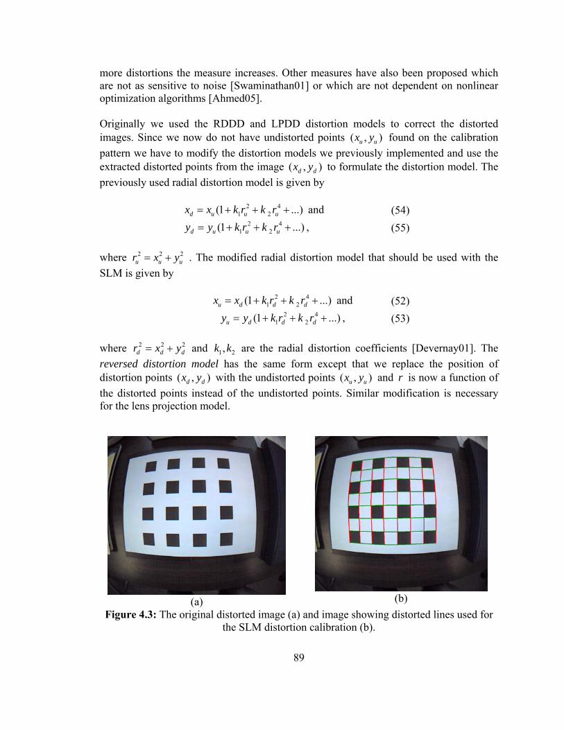
89

more distortions the measure increases. Other measures have also been proposed which are not as sensitive to noise [Swaminathan01] or which are not dependent on nonlinear optimization algorithms [Ahmed05]. Originally we used the RDDD and LPDD distortion models to correct the distorted images. Since we now do not have undistorted points ( , )u ux y found on the calibration pattern we have to modify the distortion models we previously implemented and use the extracted distorted points from the image ( , )d dx y to formulate the distortion model. The previously used radial distortion model is given by

2 41 2(1 ...)d u u ux x k r k r= + + + and (54)

2 41 2(1 ...)d u u uy y k r k r= + + + , (55)

where 2 2 2

u u ur x y= + . The modified radial distortion model that should be used with the SLM is given by

2 41 2(1 ...)u d d dx x k r k r= + + + and (52)

2 41 2(1 ...)u d d dy y k r k r= + + + , (53)

where 222

ddd yxr += and 1 2,k k are the radial distortion coefficients [Devernay01]. The reversed distortion model has the same form except that we replace the position of distortion points ( , )d dx y with the undistorted points ( , )u ux y and r is now a function of the distorted points instead of the undistorted points. Similar modification is necessary for the lens projection model.

(a)

(b)

Figure 4.3: The original distorted image (a) and image showing distorted lines used for the SLM distortion calibration (b).

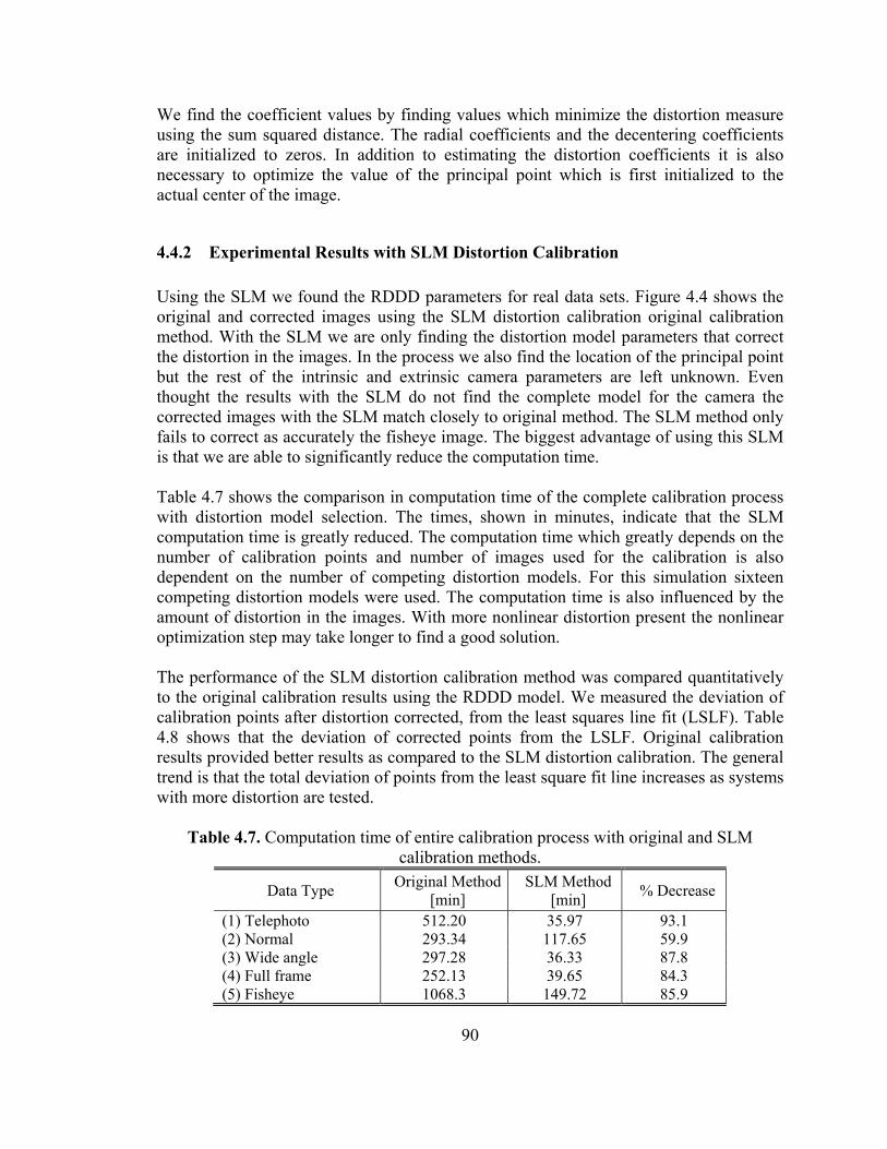
90

We find the coefficient values by finding values which minimize the distortion measure using the sum squared distance. The radial coefficients and the decentering coefficients are initialized to zeros. In addition to estimating the distortion coefficients it is also necessary to optimize the value of the principal point which is first initialized to the actual center of the image.

4.4.2 Experimental Results with SLM Distortion Calibration Using the SLM we found the RDDD parameters for real data sets. Figure 4.4 shows the original and corrected images using the SLM distortion calibration original calibration method. With the SLM we are only finding the distortion model parameters that correct the distortion in the images. In the process we also find the location of the principal point but the rest of the intrinsic and extrinsic camera parameters are left unknown. Even thought the results with the SLM do not find the complete model for the camera the corrected images with the SLM match closely to original method. The SLM method only fails to correct as accurately the fisheye image. The biggest advantage of using this SLM is that we are able to significantly reduce the computation time. Table 4.7 shows the comparison in computation time of the complete calibration process with distortion model selection. The times, shown in minutes, indicate that the SLM computation time is greatly reduced. The computation time which greatly depends on the number of calibration points and number of images used for the calibration is also dependent on the number of competing distortion models. For this simulation sixteen competing distortion models were used. The computation time is also influenced by the amount of distortion in the images. With more nonlinear distortion present the nonlinear optimization step may take longer to find a good solution. The performance of the SLM distortion calibration method was compared quantitatively to the original calibration results using the RDDD model. We measured the deviation of calibration points after distortion corrected, from the least squares line fit (LSLF). Table 4.8 shows that the deviation of corrected points from the LSLF. Original calibration results provided better results as compared to the SLM distortion calibration. The general trend is that the total deviation of points from the least square fit line increases as systems with more distortion are tested.

Table 4.7. Computation time of entire calibration process with original and SLM calibration methods.

Data Type Original Method[min]

SLM Method [min] % Decrease

(1) Telephoto 512.20 35.97 93.1 (2) Normal 293.34 117.65 59.9 (3) Wide angle 297.28 36.33 87.8 (4) Full frame 252.13 39.65 84.3 (5) Fisheye 1068.3 149.72 85.9

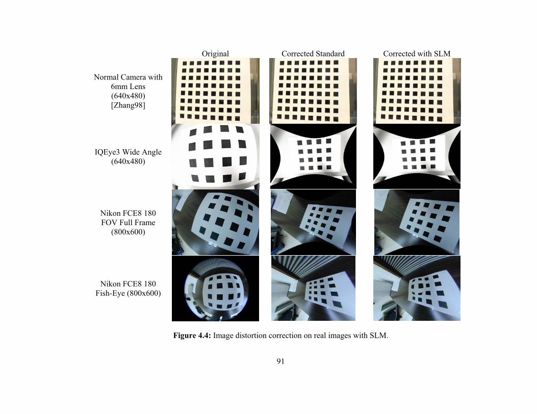
91

Original Corrected Standard Corrected with SLM

Normal Camera with 6mm Lens (640x480) [Zhang98]

IQEye3 Wide Angle (640x480)

Nikon FCE8 180 FOV Full Frame

(800x600)

Nikon FCE8 180 Fish-Eye (800x600)

Figure 4.4: Image distortion correction on real images with SLM.

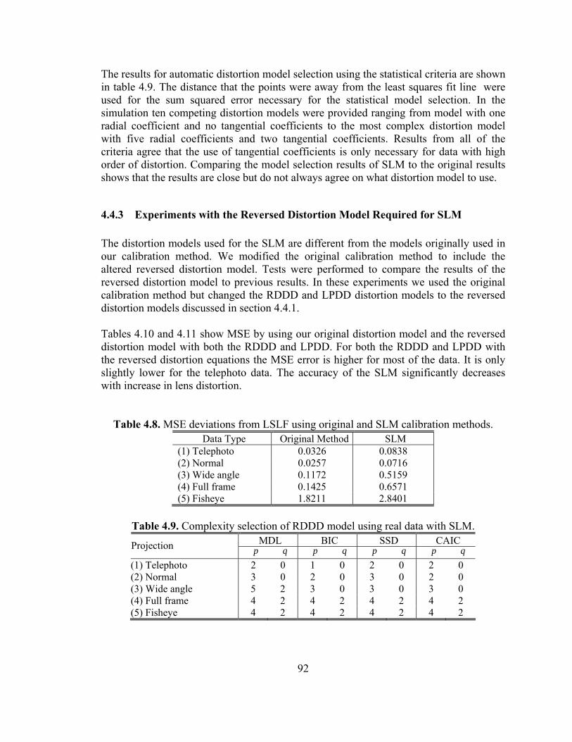
92

The results for automatic distortion model selection using the statistical criteria are shown in table 4.9. The distance that the points were away from the least squares fit line were used for the sum squared error necessary for the statistical model selection. In the simulation ten competing distortion models were provided ranging from model with one radial coefficient and no tangential coefficients to the most complex distortion model with five radial coefficients and two tangential coefficients. Results from all of the criteria agree that the use of tangential coefficients is only necessary for data with high order of distortion. Comparing the model selection results of SLM to the original results shows that the results are close but do not always agree on what distortion model to use.

4.4.3 Experiments with the Reversed Distortion Model Required for SLM The distortion models used for the SLM are different from the models originally used in our calibration method. We modified the original calibration method to include the altered reversed distortion model. Tests were performed to compare the results of the reversed distortion model to previous results. In these experiments we used the original calibration method but changed the RDDD and LPDD distortion models to the reversed distortion models discussed in section 4.4.1. Tables 4.10 and 4.11 show MSE by using our original distortion model and the reversed distortion model with both the RDDD and LPDD. For both the RDDD and LPDD with the reversed distortion equations the MSE error is higher for most of the data. It is only slightly lower for the telephoto data. The accuracy of the SLM significantly decreases with increase in lens distortion.

Table 4.8. MSE deviations from LSLF using original and SLM calibration methods. Data Type Original Method SLM

(1) Telephoto 0.0326 0.0838 (2) Normal 0.0257 0.0716 (3) Wide angle 0.1172 0.5159 (4) Full frame 0.1425 0.6571 (5) Fisheye 1.8211 2.8401

Table 4.9. Complexity selection of RDDD model using real data with SLM.

MDL BIC SSD CAIC Projection p q p q p q p q (1) Telephoto 2 0 1 0 2 0 2 0 (2) Normal 3 0 2 0 3 0 2 0 (3) Wide angle 5 2 3 0 3 0 3 0 (4) Full frame 4 2 4 2 4 2 4 2 (5) Fisheye 4 2 4 2 4 2 4 2

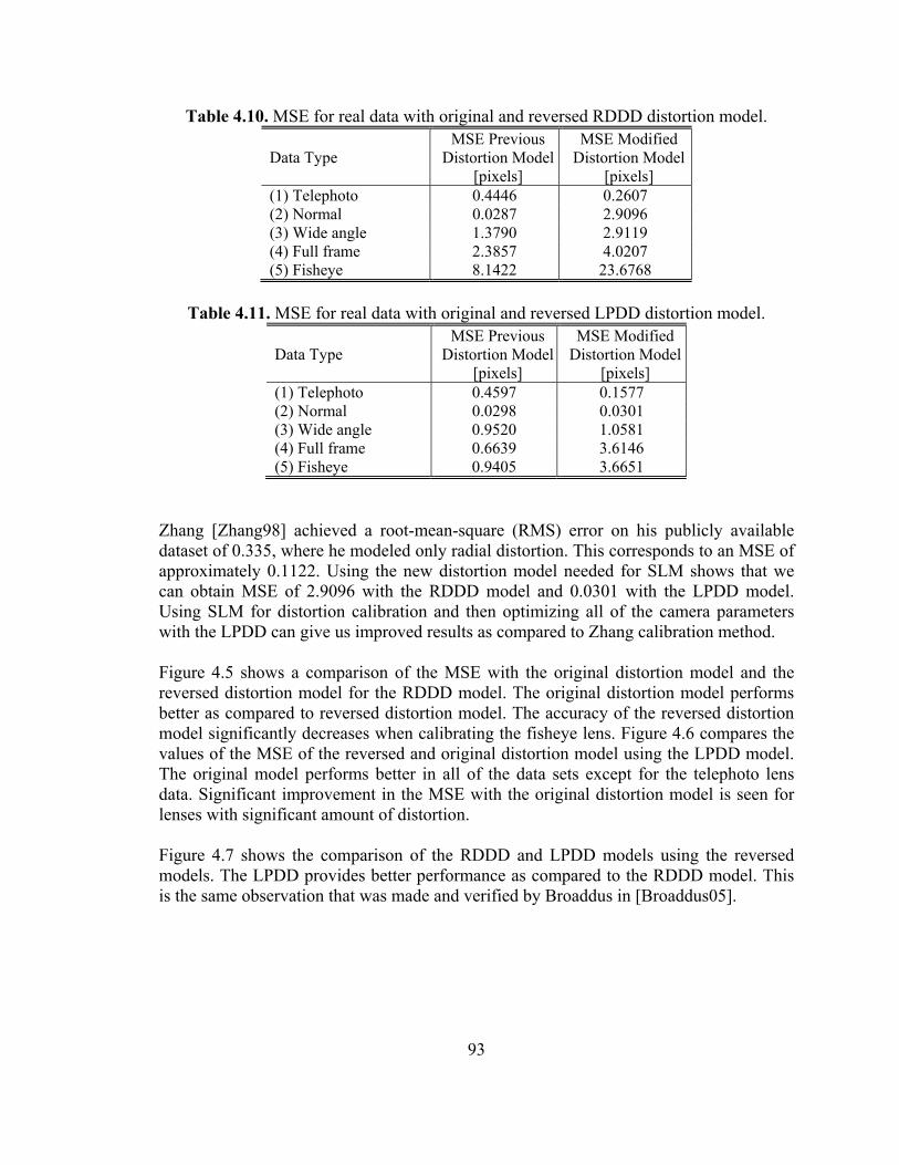
93

Table 4.10. MSE for real data with original and reversed RDDD distortion model.

Data Type MSE Previous

Distortion Model[pixels]

MSE Modified Distortion Model

[pixels] (1) Telephoto 0.4446 0.2607 (2) Normal 0.0287 2.9096 (3) Wide angle 1.3790 2.9119 (4) Full frame 2.3857 4.0207 (5) Fisheye 8.1422 23.6768

Table 4.11. MSE for real data with original and reversed LPDD distortion model.

Data Type MSE Previous

Distortion Model[pixels]

MSE Modified Distortion Model

[pixels] (1) Telephoto 0.4597 0.1577 (2) Normal 0.0298 0.0301 (3) Wide angle 0.9520 1.0581 (4) Full frame 0.6639 3.6146 (5) Fisheye 0.9405 3.6651

Zhang [Zhang98] achieved a root-mean-square (RMS) error on his publicly available dataset of 0.335, where he modeled only radial distortion. This corresponds to an MSE of approximately 0.1122. Using the new distortion model needed for SLM shows that we can obtain MSE of 2.9096 with the RDDD model and 0.0301 with the LPDD model. Using SLM for distortion calibration and then optimizing all of the camera parameters with the LPDD can give us improved results as compared to Zhang calibration method. Figure 4.5 shows a comparison of the MSE with the original distortion model and the reversed distortion model for the RDDD model. The original distortion model performs better as compared to reversed distortion model. The accuracy of the reversed distortion model significantly decreases when calibrating the fisheye lens. Figure 4.6 compares the values of the MSE of the reversed and original distortion model using the LPDD model. The original model performs better in all of the data sets except for the telephoto lens data. Significant improvement in the MSE with the original distortion model is seen for lenses with significant amount of distortion. Figure 4.7 shows the comparison of the RDDD and LPDD models using the reversed models. The LPDD provides better performance as compared to the RDDD model. This is the same observation that was made and verified by Broaddus in [Broaddus05].

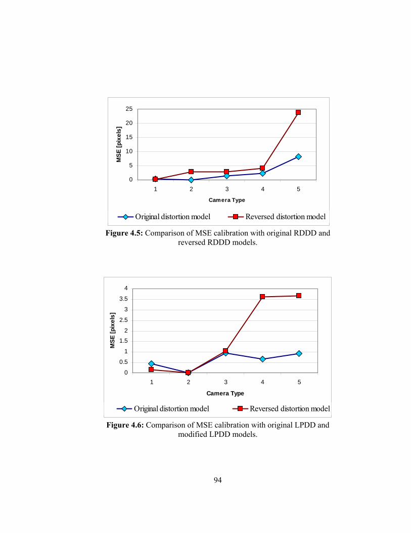
94

0

5

10

15

20

25

1 2 3 4 5

Camera Type

MSE

[pix

els]

Original distortion model Reversed distortion model

Figure 4.5: Comparison of MSE calibration with original RDDD and reversed RDDD models.

0

0.5

1

1.5

2

2.5

3

3.5

4

1 2 3 4 5

Camera Type

MSE

[pix

els]

Original distortion model Reversed distortion model

Figure 4.6: Comparison of MSE calibration with original LPDD and modified LPDD models.

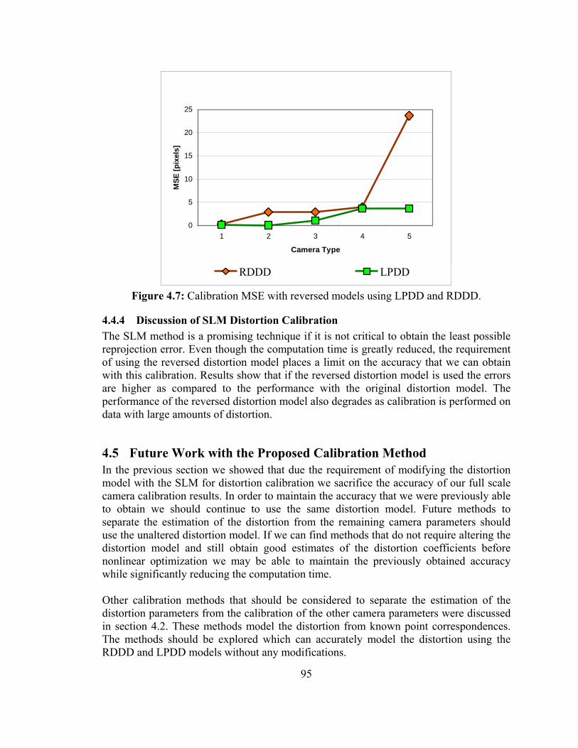
95

0

5

10

15

20

25

1 2 3 4 5

Camera Type

MSE

[pix

els]

RDDD LPDD

Figure 4.7: Calibration MSE with reversed models using LPDD and RDDD.

4.4.4 Discussion of SLM Distortion Calibration The SLM method is a promising technique if it is not critical to obtain the least possible reprojection error. Even though the computation time is greatly reduced, the requirement of using the reversed distortion model places a limit on the accuracy that we can obtain with this calibration. Results show that if the reversed distortion model is used the errors are higher as compared to the performance with the original distortion model. The performance of the reversed distortion model also degrades as calibration is performed on data with large amounts of distortion.

4.5 Future Work with the Proposed Calibration Method In the previous section we showed that due the requirement of modifying the distortion model with the SLM for distortion calibration we sacrifice the accuracy of our full scale camera calibration results. In order to maintain the accuracy that we were previously able to obtain we should continue to use the same distortion model. Future methods to separate the estimation of the distortion from the remaining camera parameters should use the unaltered distortion model. If we can find methods that do not require altering the distortion model and still obtain good estimates of the distortion coefficients before nonlinear optimization we may be able to maintain the previously obtained accuracy while significantly reducing the computation time. Other calibration methods that should be considered to separate the estimation of the distortion parameters from the calibration of the other camera parameters were discussed in section 4.2. These methods model the distortion from known point correspondences. The methods should be explored which can accurately model the distortion using the RDDD and LPDD models without any modifications.

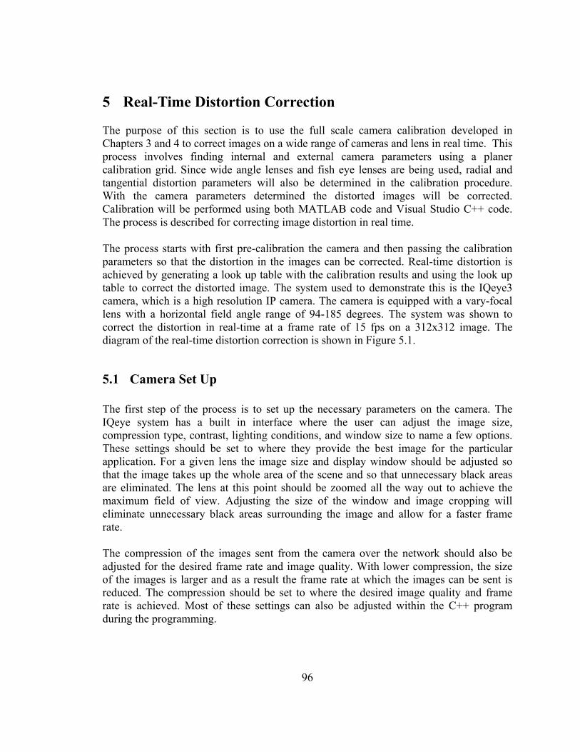
96

5 Real-Time Distortion Correction

The purpose of this section is to use the full scale camera calibration developed in Chapters 3 and 4 to correct images on a wide range of cameras and lens in real time. This process involves finding internal and external camera parameters using a planer calibration grid. Since wide angle lenses and fish eye lenses are being used, radial and tangential distortion parameters will also be determined in the calibration procedure. With the camera parameters determined the distorted images will be corrected. Calibration will be performed using both MATLAB code and Visual Studio C++ code. The process is described for correcting image distortion in real time.

The process starts with first pre-calibration the camera and then passing the calibration parameters so that the distortion in the images can be corrected. Real-time distortion is achieved by generating a look up table with the calibration results and using the look up table to correct the distorted image. The system used to demonstrate this is the IQeye3 camera, which is a high resolution IP camera. The camera is equipped with a vary-focal lens with a horizontal field angle range of 94-185 degrees. The system was shown to correct the distortion in real-time at a frame rate of 15 fps on a 312x312 image. The diagram of the real-time distortion correction is shown in Figure 5.1.

5.1 Camera Set Up The first step of the process is to set up the necessary parameters on the camera. The IQeye system has a built in interface where the user can adjust the image size, compression type, contrast, lighting conditions, and window size to name a few options. These settings should be set to where they provide the best image for the particular application. For a given lens the image size and display window should be adjusted so that the image takes up the whole area of the scene and so that unnecessary black areas are eliminated. The lens at this point should be zoomed all the way out to achieve the maximum field of view. Adjusting the size of the window and image cropping will eliminate unnecessary black areas surrounding the image and allow for a faster frame rate. The compression of the images sent from the camera over the network should also be adjusted for the desired frame rate and image quality. With lower compression, the size of the images is larger and as a result the frame rate at which the images can be sent is reduced. The compression should be set to where the desired image quality and frame rate is achieved. Most of these settings can also be adjusted within the C++ program during the programming.

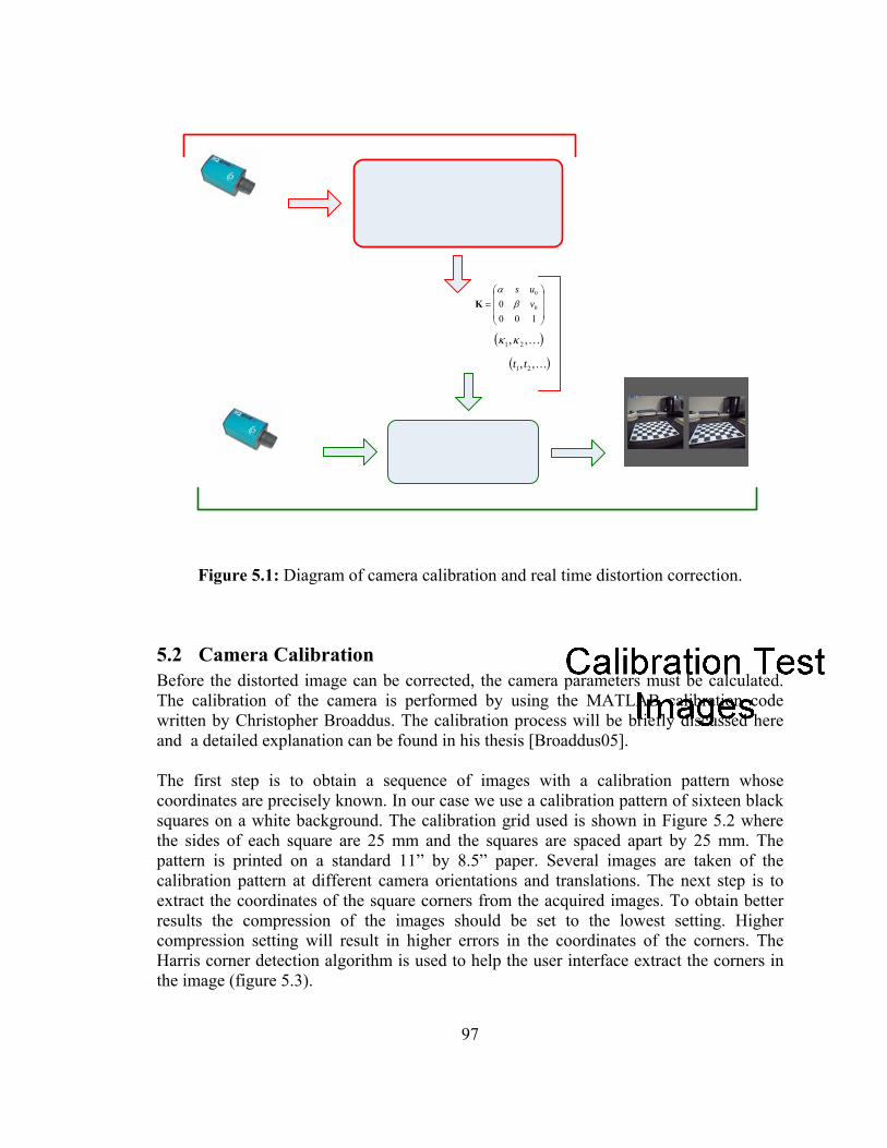
97

5.2 Camera Calibration Before the distorted image can be corrected, the camera parameters must be calculated. The calibration of the camera is performed by using the MATLAB calibration code written by Christopher Broaddus. The calibration process will be briefly discussed here and a detailed explanation can be found in his thesis [Broaddus05]. The first step is to obtain a sequence of images with a calibration pattern whose coordinates are precisely known. In our case we use a calibration pattern of sixteen black squares on a white background. The calibration grid used is shown in Figure 5.2 where the sides of each square are 25 mm and the squares are spaced apart by 25 mm. The pattern is printed on a standard 11” by 8.5” paper. Several images are taken of the calibration pattern at different camera orientations and translations. The next step is to extract the coordinates of the square corners from the acquired images. To obtain better results the compression of the images should be set to the lowest setting. Higher compression setting will result in higher errors in the coordinates of the corners. The Harris corner detection algorithm is used to help the user interface extract the corners in the image (figure 5.3).

⎟⎟⎟

⎠

⎞

⎜⎜⎜

⎝

⎛=

1000 0

0

vus

βα

K

( )…,, 21 κκ

( )…,, 21 tt

Figure 5.1: Diagram of camera calibration and real time distortion correction.

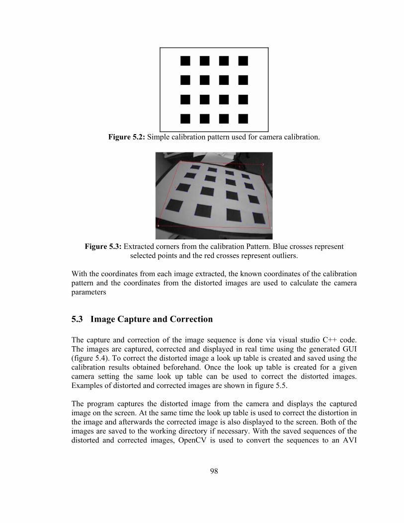
98

Figure 5.2: Simple calibration pattern used for camera calibration.

Figure 5.3: Extracted corners from the calibration Pattern. Blue crosses represent

selected points and the red crosses represent outliers. With the coordinates from each image extracted, the known coordinates of the calibration pattern and the coordinates from the distorted images are used to calculate the camera parameters

5.3 Image Capture and Correction The capture and correction of the image sequence is done via visual studio C++ code. The images are captured, corrected and displayed in real time using the generated GUI (figure 5.4). To correct the distorted image a look up table is created and saved using the calibration results obtained beforehand. Once the look up table is created for a given camera setting the same look up table can be used to correct the distorted images. Examples of distorted and corrected images are shown in figure 5.5. The program captures the distorted image from the camera and displays the captured image on the screen. At the same time the look up table is used to correct the distortion in the image and afterwards the corrected image is also displayed to the screen. Both of the images are saved to the working directory if necessary. With the saved sequences of the distorted and corrected images, OpenCV is used to convert the sequences to an AVI

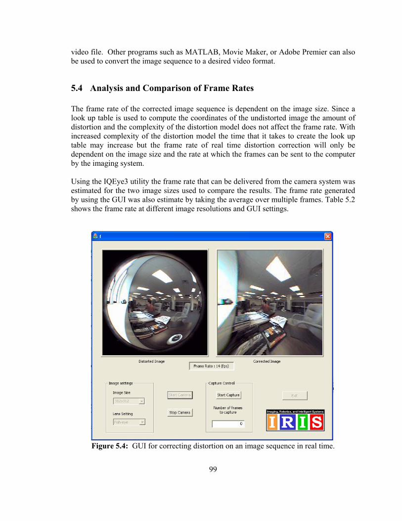
99

video file. Other programs such as MATLAB, Movie Maker, or Adobe Premier can also be used to convert the image sequence to a desired video format.

5.4 Analysis and Comparison of Frame Rates The frame rate of the corrected image sequence is dependent on the image size. Since a look up table is used to compute the coordinates of the undistorted image the amount of distortion and the complexity of the distortion model does not affect the frame rate. With increased complexity of the distortion model the time that it takes to create the look up table may increase but the frame rate of real time distortion correction will only be dependent on the image size and the rate at which the frames can be sent to the computer by the imaging system. Using the IQEye3 utility the frame rate that can be delivered from the camera system was estimated for the two image sizes used to compare the results. The frame rate generated by using the GUI was also estimate by taking the average over multiple frames. Table 5.2 shows the frame rate at different image resolutions and GUI settings.

Figure 5.4: GUI for correcting distortion on an image sequence in real time.

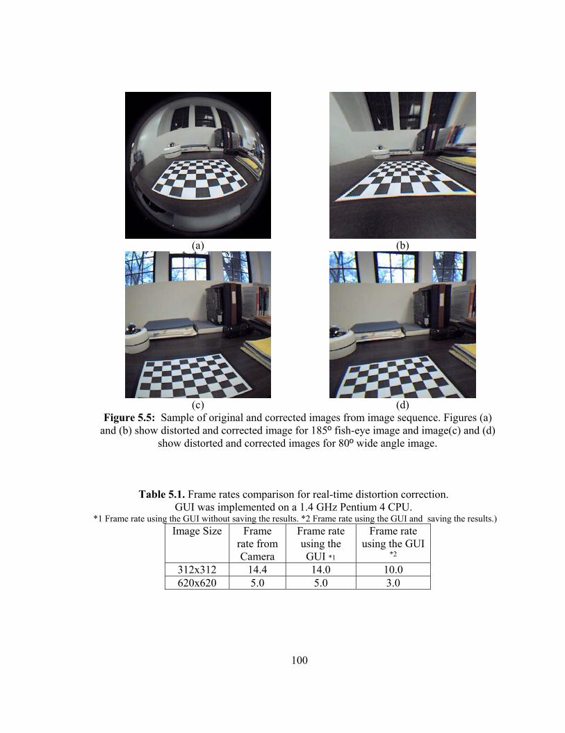
100

(a)

(b)

(c)

(d)

Figure 5.5: Sample of original and corrected images from image sequence. Figures (a) and (b) show distorted and corrected image for 185º fish-eye image and image(c) and (d)

show distorted and corrected images for 80º wide angle image.

Table 5.1. Frame rates comparison for real-time distortion correction. GUI was implemented on a 1.4 GHz Pentium 4 CPU.

*1 Frame rate using the GUI without saving the results. *2 Frame rate using the GUI and saving the results.)Image Size Frame

rate from Camera

Frame rate using the GUI *1

Frame rate using the GUI

*2 312x312 14.4 14.0 10.0 620x620 5.0 5.0 3.0

101

6 CONCLUSIONS

6.1 Summary In this thesis we have completed, improved, and evaluated a universal camera calibration method. The work is a direct continuation of previous research performed by [Broaddus05]. We have extensively tested the performance of this method on both real and synthetic data. The results were extended to include lenses which were not tested previously. Some of the limitations witch were observed during the testing were addressed and results now include the successful calibration of vari-focal telephoto lenses. We have done an extensive survey of recent advances in the area of distortion calibration for wide angle and fish-eye lenses. Based on this survey we have proposed a modification to the previous method to separate the estimation of the distortion parameters from the estimation of other parameters. In this step we have shown that separating the calibration can significantly improve the computation time. Several techniques were explored to perform the distortion calibration. It is shown that these techniques can successfully calibrate the distortion of the camera but the challenge is in finding a method which can be easily adapted to our previous method’s distortion models.

6.2 Contributions Contributions include:

• Testing and comparing the original calibration method o Tested calibration performance on real and synthetic data of telephoto

lenses. o Verified and compared the successful selection of distortion model with

synthetic data for five different criteria. • Determined the limitations of the calibration procedure for telephoto lenses and

modified the previous method to accurately calibrate systems with large focal length.

• Proposed and presented a new calibration method which separates the estimation of the distortion parameters from the rest of the camera parameters in order to achieve faster calibration.

6.3 Future Work As imaging technology and manufacturing techniques progress we will have fewer imperfections in the imaging systems but we will still continue to need accurate models

102

to efficiently describe the way cameras project 3D world scenes to a 2D image plane. The work of this thesis has shown the successful performance of a complete calibration method which can find the model parameters of many different imaging systems regardless of distortion or projection. Future work in the area of camera calibration should continue to advance with the criteria proposed by Broaddus [Broaddus05] and in this thesis. These criteria include that the methods be complete, simple, and universal calibration method. In the ongoing research many calibration methods focus on developing approaches which will work on unique imaging systems. The drawback with these methods is that with particular imaging systems certain assumptions are made which can not be easily extended to other systems. The advantage of calibration methods such as the one presented in this thesis is that they can be used with a wide range of imaging systems without any prior assumptions or knowledge of parameters. Since the early days of photogrammetry, advances in technology and numerical analysis methods have allowed significant improvements in the area of calibrating digital cameras. The numerical methods used in the estimation of parameters should continue to be improved for both computation time and accuracy. With competing approaches to solve for these parameters, automatic selection criteria should be used to determine the best approach for the given data set or application. The optimization of the parameters also needs special attention. Competing optimization techniques should be compared for camera calibration. Tests should be done to determine the optimal parameters to control the optimization. Improved optimization procedures would allow for faster, more accurate, and stable results. As part of future work we should continue to find better techniques to separate the accurate estimation of camera parameters into separate stages. It was shown in this thesis that we can successfully separate the estimation of distortion coefficients from the rest of camera parameters. This allows us to significantly reduce the computation time for selecting the best distortion model before nonlinear optimization. In addition to reducing computation time there is the potential to increase the accuracy if we can implement distortion calibration with the most accurate distortion model. Developing methods to accurately estimate individual camera parameters in separate stages has the potential to provide the necessary accuracy to omit these parameters from the nonlinear optimization. This would significantly reduce the computation complexity of the camera calibration.

103

REFERENCES

104

[Agrawal03] M. Agrawal and L. Davis, “Camera calibration using spheres: A semidefinite programming approach,” in ICCV, pp. 782-789, 2003.

[Ahmed05] M, Ahmed and A. Farag, “Nonmetric Calibration of Camera Lens

Distortion: Differential Methods and Robust Estimation,” in IEEE Transactions on Image Processing, vol. 14, Is. 8, pp. 1215-1230, August 2005.

[Ahmed00] Ahmed, M.T.; Farag, A.A., "A neural optimization framework for

zoom lens camera calibration," Computer Vision and Pattern Recognition, 2000. Proceedings. IEEE Conference on, vol.1, no.pp.403-409 vol.1, 2000.

[Akaike74] H. Akaike, “A New Look at the Statistical Model Identification,” In

IEEE Transactions on Automatic Control, 19(6), 1974. [Basu95] Basu and S. Licardie, “Alternative models for fisheye lenses,”

Pattern Recognition Lett., 16(4), pp. 433-441, 1995. [Bakstein02a] H. Bakstein and T. Pajdla, “Panoramic Mosaicing with a 180/spl

deg/ Field of View Lens,” in Proceedingsf Third Workshop on Omnidirectianl Vision, pp. 60-67, 2002.

[Bakstein02b] H. Bakstein and T. Pajdla, “Calibration of a fish eye lens with field

of view larger than 180deg”, CVWW'02, PRIP Wien, Austria, February 2002.

[Barajas06] Barajas, L. G. “Machine Vision Glossary”, 25 May 2006,

http://en.wikipedia.org/wiki/Machine_Vision_Glossary [Barreto04] J. Barreto and K. Daniilidis, “Wide Area Multiple Camera

Calibration and Estimation of Radial Distortion,” in Workshop on Omidirectional Vision and Camera Networks, Prague, Czech rep., pp. 5-16, 2004.

[Barreto03] J. P. Barreto and H. Araujo, “Paracatadioptric Camera Calibration

Using Lines,” in Proceedings Ninth IEEE International Conference on Computer Vision , vol. 2 pp. 1359-1964 , 13-16 October 2003.

[Booth36] Booth, L. “The Telephoto Lens.” Proc. Opt. Conv. 861, 1936. [Brauer-Burchard01] C. Brauer-Burchardt and K. Voss, “A New Algorithm to Correct

Fish-Eye and Strong Wide-Angle-Lens-Distortion from Single Images,” in Proceedings International Conference on Image Processing, vol. 1, pp. 225-228, 2001.

105

[Bozdogan87] H. Bozdogan, “Model Selection and Akaike’s Information

Criterion,” Psychmetrika, 53(3), pp. 345-370, 1987. [Broaddus05] C. Broaddus, “Universal Geometric Camera Calibration with

Statistical Model Selection,” Masters Thesis, Department of Electrical Engineering, The University of Tennessee, Knoxville, TN 2005.

[Brown71] D. C. Brown, “Close-range camera calibration”, Photogrammetric

Engineering, vol. 37, no. 8, pp. 323-344, 1971. [Canero02] C. Canero, F. Vilarino, J. Mauri, and P. Radeva, “Predictive

(un)distortion model and 3D reconstruction by biplane snakes,” in IEEE Trans. Med. Imag., vol. 21, pp. 1188–1201, Sept. 2002.

[Chen00] Yong-Sheng Chen; Shen-Wen Shih; Yi-Ping Hung; Chiou-Shann

Fuh, "Camera calibration with a motorized zoom lens," Pattern Recognition, 2000. Proceedings. 15th International Conference on, vol.4, no.pp.495-498 vol.4, 2000.

[Claus05] D. Claus and A. W. Fitzgibbon, “A rational function lens distortion

model for general cameras,” in CVPR 205 IEEE Computer Society Conference on Computer Vision and Pattern Recognition, Vol. 1, pp. 213-219, 20-25 June 2005.

[Collins99] Collins, R.T.; Tsin, Y., "Calibration of an outdoor active camera

system," Computer Vision and Pattern Recognition, 1999. IEEE Computer Society Conference on, vol.1, no.pp.-534 Vol. 1, 1999.

[Conrady19] A. Conrady, “Decentering lens systems”, Monthly Notices of the

Royal Astronomical Society of America, 79:951–954, 1919. [Criminisi99] A. Criminisi, I. Reid, and A. Zisserman, “Single view metrology,” in

IEEE International Conference on Computer Vision 1999, vol. 1, pp. 434-441, 1999.

[Cucchiara03] R. Cucchiara, C. Grana, R. Vezzani, “A Hough transform-based

method for radial lens distortion correction,” in 2003 Proceedings of 12th International Conference on Image Analysis and Processing, pp. 182-187, 17-19 September 2003.

[Devernay01] F. Devernay and O. Faugeras, “Straight lines have to be straight:

Automatic calibration and removal of distortion from scenes of

106

structured environments,” Machine Vision and Applications, 13(1), pp. 14-24, 2001.

[El-Melegy03] M. T. El-Melegy and A. A. Farag, “Nonmetric lens distortion

calibration: closed-form solutions, robust estimation and model selection,” in Ninth IEEE Int. Conf. on Computer Vision, 2003. vol. 1, pp. 554-559, 13-16 Oct. 2003.

[Fitzgibbon01] A. W. Fitzgibbon, “Simultaneous linear estimation of multiple view

geometry and lens distortion,” in Proceedings of the 2001 IEEE Computer Society Conf. on Computer Vision and Pattern Recognition, CVPR-2001, vol. 1, pp. I-125 – I-132, 2001.

[Fleck95] M.M. Fleck, “ Perspective projection: The wrong imaging model,”

Technical Report TR 95-01, Computer Science Dept., University of Iowa, 1995.

[Geyer02] C. Geyer and K. Daniilidis, “Paracatadioptric Camera Calibration,”

in IEEE Transactions on Pattern Analysis and Machine Intelligence, Vol. 24, Iss. 5, pp. 687-695, May 2002.

[Gheissari03] N. Gheissari and A. Bab-Hadiashar, “Model selection criteria in

computer vision: are they different?” Proc. VIIth Digital Image Computing: Techniques and Applications, pp. 185-194, 10-12 Dec. 2003.

[Graf05] S. Graf, T. Hanning, “Analytically solving radial distortion

parameters”, in CVPR 2005 IEEE computer Society Conference on Computer Vision and Pattern Recognition, Vol. 2, pp. 20-26, June 2005.

[Hartley05] R. Hartley and S. B. Kang, “Parameter-free radial distortion

correction with center of distortion estimation,” in Proc. ICCV-2005, Oct. 2005.

[Hartley04] R. Hartley and A. Zisserman, Multiple View Geometry in Computer

Vision, 2nd Edition, Cambridge University Press, 2004. [Hartley97] R. I. Hartley and T. Saxena, “The cubic rational polynomial camera

model,” in Bibliography 593 Proc. DARPA Image Understanding Workshop, pp. 649-653, 1997.

[Heikkila00] J. Heikkila, “Geometric Camera Calibration Using Circular Control

Points,” In IEEE Transactions on Pattern Analysis and Machine Intelligence, 22(10), pp. 1066-1077, October 2000.

107

[Heikkila97] J. Heikkila and O. Silven, “A Four-Step Camera Calibration

Procedure with Implicit Image Correction,” In Proceedings of IEEE Conference on Computer Vision and Pattern Recognition, pp.1106-1112, 1997.

[Hemayed03] E. Hemayed, “A survey of camera self-calibration,” in Proceedings

IEEE Conference on Advanced Video and Signal Based Surveillance, 2003, pp. 351-357, 21-22 July 2003.

[Ishii03] C. Ishii, Y. Sudo, H. Hashimoto, “An image conversion algorithm

from fish eye image to perspective image for human eyes,” in AIM 2003 IEEE/ASME International Conference on Advanced Intelligent Mechatronics, Vol. 2, pp. 1009-1014, 20-24 July 2003.

[Kang01] S.B. Kang, “Radial distortion snakes,” IEICE Trans. Inf. & Syst.,

vol. E84-D, No. 12, pp. 1603-1611, Dec. 2001. [Kannala04] J. Kannala and S. Brandt, “A Generic Camera Calibration Method

for Fish-Eye Lenses,” in Proceedings of the 17th International Conference on Pattern Recognition, ICPR 2004, vol. 1, pp. 10-13, 23-16 August 2004.

[Kinoshita00] K. Kinoshita and L. Lindenbaum, “Camera model selection based on

geometric AIC,” in Proc. IEEE Conf. on Computer Vision and Pattern Recognition, 2000, vol. 2, pp. 514-519.

[Lenz87] R. Lenz and R. Tsai, “Techniques for Calibration of the Scale Factor

and Image Center for High Accuracy 3D Machine Vision Metrology”, In Proceedings of the IEEE International Conference on Robotics and Automation, pp. 68-75, Raleigh NC, 1987.

[Li96] Mangling Li; Laves, J.-M., "Some aspects of zoom lens camera

calibration," Pattern Analysis and Machine Intelligence, IEEE Transactions on, vol.18, no.11pp.1105-1110, Nov 1996.

[Li05] H. Li and R. Hartley, “A non-iterative method for correcting lens

distortion from nine point correspondences,” in Proc. 6th Workshop on Omnidirectional Vision, 2005.

[Ma06] L. Ma, Y. Q. Chen, and K. L. Moore, “Analytical Piecewise radial

distortion model for precision camera calibration,” IEE Proc. –Vies. Image Signal Process., Vol. 153 No. 4, August 2006.

108

[Mallon04] J. Mallon and P.F. Whelan, “Precise radial un-distortion of images,” in ICPR 2004 Proceedings of the 17th International Conference on Pattern Recognition, Vol. 1, pp. 18-21, 23-26 Aug, 2004.

[Marshall06] Marshall, P. “Using Telephoto Lenses”, 06 December, 2006,

www.photography.about.com/od/basics/a/bptelephoto.htm [Medioni05] G. Medioni and S. B. Kang, Emerging Topics in Computer Vision,

Prentice Hall, 2005. [Meng04] Y. Meng and H. Zhuang, “What you see is what you get [self-

calibration camera lens distortion],” IEEE Robotics and Automation Magazine, Vol. 11, Iss. 4, pp. 123-127, December 2004.

[Micusik03] B. Micusik and T. Pajdla, “Estimation of omnidirectional camera

model from epipolar geometry,” Computer Vision and Pattern Recognition, 2003. Proceedings. 2003 IEEE Computer Society Conference on , vol.1, no.pp. I-485- I-490 vol.1, 18-20 June 2003.

[Ngo05] H. T. Ngo and V. K. Asari, “A Pipelined Architecture for Real-Time

Correction of Barrel Distortion in Wide-Angle Camera Images,” in IEEE Transactions on Circuits and Systems for Video Technology, vol. 15, Iss. 3, pp. 436-444, March 2005.

[Ramalingam05] S. Ramalingam, et al., “Towards complete generic camera

calibration,” in CVPR-2005, IEEE Computer Society Conf. on Computer Vision and Pattern Recognition, 2005, vol. 1, pp. 1093-1098.

[Rissanen78] J. Rissanen, “Modeling by Shortest Data Description,” Automatica,

vol. 14, pp. 465-471, 1978. [Sagawa05] R. Sagawa, M. Takatsuji, T. Echigo, Y. Yagi, "Calibration of lens

distortion by structured-light scanning," Intelligent Robots and Systems, 2005. (IROS 2005). 2005 IEEE/RSJ Int. Conf on, pp. 832- 837, 2-6 Aug. 2005.

[Schwarz78] G. Schwarz, “Estimating the Dimension of a Model,” Annals of

Statistics, vol. 6, pp. 461-464, 1978. [Shah96] S. Shah, J. K. Aggarwal, “Intrinsic Parameter Calibration Procedure

for a (High-Distortion) Fish-Eye Lens Camera with Distortion Model and Accuracy Estimation,” Pattern Recognition 29, No. 11, pp. 1175-1788, November 1995.

109

[Shah94] S. Shah and J. K. Aggarwal “A simple calibration procedure for fish-eye (high distortion) lens camera,” in 1994 Proceedings IEEE International conference on Robotics and Automation, vol. 4, pp. 3422-3427, 8-13 May 1994.

[Shih94] Sheng-Wen Shih; Yi-Ping Hung; Wei-Song Lin, "Head/eye

calibration of a binocular head by use of single calibration point," Image Analysis and Interpretation, 1994., Proceedings of the IEEE Southwest Symposium on , vol., no.pp.154-159, 21-24 Apr 1994.

[Shih98] Sheng-Wen Shih; Yi-Ping Hung; Wei-Song Lin, "Calibration of an

active binocular head," Systems, Man and Cybernetics, Part A, IEEE Transactions on , vol.28, no.4pp.426-442, July 1998.

[Stein97] G. P. Stein, “Lens distortion calibration using point

correspondences,” in IEEE Computer Society Conf. on Computer Vision and Pattern Recognition, 1997. pp. 602-608. 17-19 June 1997.

[Stevenson96] D. E. Stevenson and F. M. Margaret, “Nonparametric Correction of

Distortion,” in WACV ’96 Proceedings 3rd IEEE Workshop on Applications of Computer Vision, pp. 214-219, 2-4 Dec. 1996.

[Sturm05] P. Sturm, “Multi-view geometry for general camera models,” in

IEEE Computer Society Conference on Computer Vision and Pattern Recognition, CVPR 2005, Vol. 1, pp. 206-212, 2005.

[Swaminathan01] R. Swaminathan and S. K. Nayar, “Nonmetric calibration of wide-

angle lenses and polycameras,” in IEEE Transactions on Pattern Analysis and Machine Intelligence, Vol. 22, Iss. 10, pp. 172-1178, October 2000.

[Thirthala05a] S. Thirthala and M. Pollefeys, “The radial trifocal tensor: a tool for

calibrating the radial distortion of wide angle cameras,” in IEEE Computer Society Conf. on Computer Vision and Pattern Recognition, 2005, vol. 1, pp. 321-328, 20-25 June 2005.

[Thirthala05b] Thirthala, S.R.; Sinha, S.N.; Pollefeys, M., "Calibration of pan-tilt-

zoom (PTZ) cameras and omni-directional cameras," Computer Vision and Pattern Recognition, 2005. CVPR 2005. IEEE Computer Society Conference on , vol.2, pp. 1198 vol. 2-, 20-25 June 2005.

[Tordoff04] B. Tordoff and D. Murray, “The impact of radial distortion on the

self-calibration of rotating cameras,” CVIU, Vol. 96, No. 1, pp. 17-34, Oct. 2004.

110

[Tordoff00] B. Tordoff and D. Murray, “Violating rotating camera geometry:

The effect of radial distortion on self-calibration,” Proc. 15th Int’l Conf. Pattern Recognition, pp. 423-427, 2000.

[Triggs00] B. Triggs, P. F. McLauchlan, R. I. Hartley & A. W. Fitzibbon,

Bundle adjustment -- a modern synthesis, in Vision Algorithms: Theory and Practice, pp. 298--375, Springer, Berlin, (2000).

[Tsai87] R.Y. Tsai, “A versatile camera calibration technique for high-

accuracy 3D machine vision metrology using off-the-shelf TV cameras and lenses”, IEEE Journal of Robotics and Automation, vol. 3, no. 4, pp. 323-344, Aug. 1987.

[Weng92] J. Weng, P. Cohen, and M. Herniou, “Camera calibration with

distortion models and accuracy evaluation,” in IEEE Transactions on Pattern Analysis and Machine Intelligence, vol. 14, no. 10, pp. 965-980, Oct. 1992.

[Wei98] Guo-Qing Wei; Arbter, K.; Hirzinger, G., "Active self-calibration of

robotic eyes and hand-eye relationships with model identification," Robotics and Automation, IEEE Transactions on, vol.14, no.1pp.158-166, Feb 1998.

[Willson94] R.G. Willson, “Modeling and Calibration of Automated Zoom

Lenses,” PhD thesis, CMU-RI-TR-94-03, Robotics Inst., Carnegie Mellon Univ., January 1994.

[Willson93] R.G. Willson, “What is the center of the image?” Computer Vision

and Pattern Recognition, 1993. CVPR 1993. IEEE Computer Society Conference on, pp. 670 – 671, 15-17 June, 1993.

[Xu06] De Xu, You Fu Li, and Min Tan, “ Method for calibrating cameras

with large lens distortion,” SPIE, vol. 45(4), April 2006. [Ying04] X. H. Ying and Z. Y. Hu, Can We Consider Central Catadioptric

Cameras and Fisheye Cameras within a Unified Imaging Model, in Proc. European Conference on Computer Vision ( ECCV-2004), Vol. I, pp.442-455, Prague, Czech, 2004.

[Zhang05] H. Zhang, G. Zhang, K. K. Wong, “Camera calibration with spheres:

A linear approach,” in ICIP, pp. 1150-1153, 2005.

111

[Zhang00] Z. Zhang, “A flexible new Technique for camera calibration”, IEEE Tans. Pattern Analysis and Machine Intelligence, Vol. 22, No. 11, 1330C1334, Nov. 2000.

[Zhang98] Z. Zhang, “A flexible new Technique for camera calibration”,

Technical Report MSR-TR-98-71, Microsoft Research, Dec. 1998.

112

VITA Vitaliy Leonidovich Orekhov was born in Yessentuki, Russia on May 19, 1982, to Leonid Ivanovich Orekhov and Yelena Genrichovna Orekhov. His family emigrated from the former Soviet Union to East Tennessee on July 5, 1991. Vitaliy attended grade school in Morristown, TN and graduated with honors from Morristown Hamblen High School West in May 2001. Vitaliy began attending Tennessee Technological University in Cookeville, TN in August 2001. He received his B.S. in Electrical Engineering from Tennessee Tech in May 2005. While attending Tennessee Tech Vitaliy participated in Baptist Student Union, IEEE, SAE, TTU Motorsports Formula SAE, Eta Kappa Nu (HKN), and TTU Engineering Joint Council. After completing his undergraduate education he participated in NREIP program at Naval Surface Warfare Center, in Dahlgren, Virginia. Vitaliy began working as a graduate research assistant for the Imaging, Robotics, and Intelligent Systems Laboratory (IRIS) at the University of Tennessee in Knoxville, TN, in August 2006. He will be graduating with an M.S. in Electrical Engineering in August 2007.