UNCLASSIFIED

AD NUMBER

AD472558

NEW LIMITATION CHANGE

TOApproved for public release, distributionunlimited

FROMDistribution authorized to U.S. Gov't.agencies and their contractors;Administrative/Operational Use; AUG 1965.Other requests shall be referred to AirForce Flight Dynamics Lab.,Wright-Patterson AFB, OH 45433.

AUTHORITY

AFFDL ltr, 29 Dec 1971

THIS PAGE IS UNCLASSIFIED

I

SECURITYMARKING

The classified or limited status of this rpa!t applies

to each page, unless otherwise m~ted.Separate page printoutf MUST be marked accordingly.

IHIS DOCUMENT CONTAINS INFORMATION AFFECTING THE NATIONAL DEFENSE OFTHE UNITED STATES WITHIN THE MEANING OF THE ESPIONAGE LAWS, TITLE 18,U.S.C., SECTIONS 793 AND 794. THE TRANSMISSION OR THE REVELATION OFITS CONTENTS IN ANY MANNER TO AN UNAUTHORIZED PERSON IS PROHIBITED BYLAW.

NOTICE: When government or other drawings, specifications or otherdata are used for any purpose other than in connection with a defi-nitely related government procurement operation, the U. S. Governmentthereby incurs no responsibility, nor any obligation whatsoever; andthe fact that the Government may have formulated, furnished, or in anyway supplied the said drawings, specifications, or other data is notto be regarded by implication or otherwise as in any manner licensingthe holder or any other person or corporation, or conveying any eightsor permission to manufacture, use or sell any patented invention thatmay in any way be related thereto.

AFFDL-TR-65-139 i

iPREDICTION Or SPACE VEHICLE

! THERMAL CHARACTERISTICS

J. T. Bevans, et al.

S ,TRW Systems Group

sow,

TECHNICAL REPORT AFFDL-TR-66-139

AUGUST 10O6

I

DDC

Lt OCT 2' "iI

AIR FORCE FLIGHT DYNAMICS LABORATORYRENEARCH AND TECHNOLOGY DIVISION

AIR FO'CZ HYSMS COMMAND

If WRIGHTPATIMRK0 AIR FORCX SE. OHIO

NO TICES

When Government drawings, speclficatioas, or other data ar-e used fo.-an~y purpos: other than in connection with a defin-0,kely related Governmentprocuremient operation, the Uuited States Governme~nt thereby :_ncurs noresponsibility nor any oblig,,?tion whatsoever; an-d the fact that the Governmentmay have foriulated, Lurnished, or in any way supplied the said drawJigs,specifications, or other data, is not to be regarded by iraplicAtion o: other-wise as in any manner licensing the holder or any other person or corporation,or conveying any rights or permission to manufacture, use, or sell anykpatented invention that may in any way be related thereto.

Qualified users may obtain copics of this report from the DefenseDocumentation Center. The distribution of this report is limited becausetha report contains technology identifiable with itemis on the strategicewnbargo lists excluded f-om. export or re-export under U. S. Export ControlAct of 1949 (63 STA"'. 7) as amended (50 U.S.C. App. 2020.2031) as implecientadby AFR 400-10.

Copies of this report should not be returned to the Research andTechnoloy Divimion imnless return in required by security coniderations,contractual obligaticixa, or notice ^-n a specific docuaum.

iPREDICTION OF SPACE VEHICLETHERMAL CHARACTERISTICS,

TRW Systems Group JY" El L ,

TECHNICAL REEPV3.:rfLn

AIF*/6"4-_ 6L t ' 4 6

AF( 0 4

AIR FORCE FLIGHT DYNAMICS LABORATORY

RESEARCH AND TECHNOLOGY DMSIONAIR FORCE SYSTEMS OMMAND

WRIGHT-PAT'rRSON AIR FORCE BASE, OHIO

°--0

i~i,.

SFORtWORD

The following report was/prepared by TRW systems Group, under USAFContract No. AF 33(615)-1725 as part of Project 6146, Task 614617. Theprogram was edministered by the Air Force Flight Dynamics Laooratory,Research and Technology Division, Wright-Patterson Air Force Base. TheTochnical Monitor was Mr. C. J. Feldmanis.

The program was performed by J. T. Bevans, T. Ishimoto, B. R. Loya,and E. E. Luedke. Dr. D. K. Edwards of the University of California, atLos Angeles, was consultant throughout the study.

The manuscript was released by the authors 31 August 1965, forpublication as an RTD Technical Report.

This technical report has been reviewed and is approved.

Etiironmental Control BranchVehicle Euipment DivisionAF Flight Dynamics Laboratory

- -- -- . .. ., -.i - m u I i ln I

ABSTRACT

The work repor-,ed herein is the first phase of a program to improvethe prediction of spacecraft thermal performance. The study has consistedof measuring actual jo it thermal conducta:'es, correlation of themeasured joint conductances, programing an improved method of thermalradiation analysis, and performing an experimental comparison of predictedradiation exchange for a simple geor trical system.

Three types of structural and three sizes of component mounting jointswers tested and the conductances measured. A successful method ofcorrelation was developed for the unfilled component mounting joints. Alljoints were selected for their applicability to the next phase of theprogram, a thermal test of a upacecraft model.

A method of radiation analysis has been progrmed which uses directional

thermal radiation properties and accounts for the specularity and/ordiffuseness of these properties. The results of this program can bereadily incorporated into most existing thermal analysis program . Theuser has the choice of the specular, the diffuse, or the specular-diffuseassumption. The prediction of radiation exchange using these assumptionsfor simple geometrical arrangeasnts has been compared to experiment.Althoulh the results were within the overall experimental tolerances, furtherimprovement in the predicted values is believed possible.

he study has developed several important technical areas which areworthy of further evaluation. The first is the extension of the correlationtechniques to include filled component joints and filled or unfilledstructural joints. Continuation of the general measurement of joints todevelop & large knowledge of practical joint conductances in also indicated.The comparison of experimental and predicted radiation exchange has shownthat a more extensive study is needed of therm]l radiation properties todetezaine the division of these properties into specular and diffsecomponents. The non-gray error of radiation aralysis has also been shownto be an important area for further otudy.

-ii

.... _ _ __....

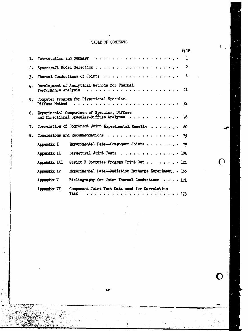
TABLE OF CONTENTS

PAGE

1. Introduction and Summary .. .. .. .. .. .. .. .. . .. . 1

2. Spacecraft Model Selection ....................... . 2

3. Thermal Conductance of Joints . . . . . . . . . . . . . . 4

4. Development of Analytical Methods for ThermalPerformance Analysis . . . . . . . . . . . . . . . . . . . . . . 21

5. Computer Program for Directional Specular-Diffuse Method . . . . . . . . . . . . . . . . . . .. . . . . 32

6. Experimental Comparison of Specular, Diffuse

and Directional Specular-Diffusen] ses .. . . . . ... 46

7. Correlation of Component Joint Experimental Results ....... 60

8. Conclusions and Recommendations . . .... . . .. ...... 75

Appendix I Experimental Datat-Coponent Joints . . . . ... 79

SAppendix 11 Structural Joint Tests .. .. .. ... . 104

AppenixIII Script F Computer Program Prnt Out . . . ..... 124 CApperdix IV Eperimental fta-lRad tion Exchare Lperimnt.. 165

Appendix V Bibl ogrps y for Joint Thermal Conductance .... 171

Appndix VI Caponent Joint Tet Data used for CorrelationTas . . . . . . . . . ..*. . . . . . . . . . 173

'V0

-I -' - '. .~I

• m lw mmm m •m Jm em mm m m

5 ILLUS ATIONS

FIGURE PAGE

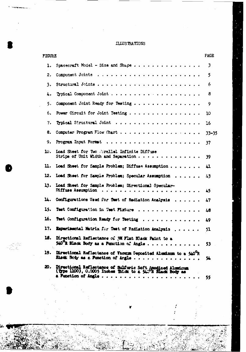
1. Spacecraft Model - Size and Shape. . . . . . . . .. .. . . . 3

2. Component Joints ........... . . o . # . . * . .. . . . . . 5

3. Structural Joints ...... .. ....................... 6

4. Typical Component Joint . . . ........... . . . . 8

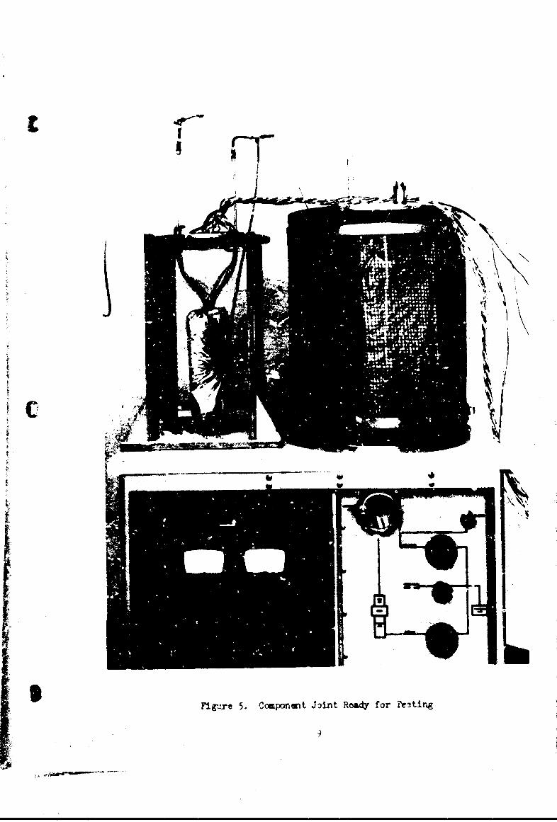
5. Component Joint Ready for Testing .. .............. 9

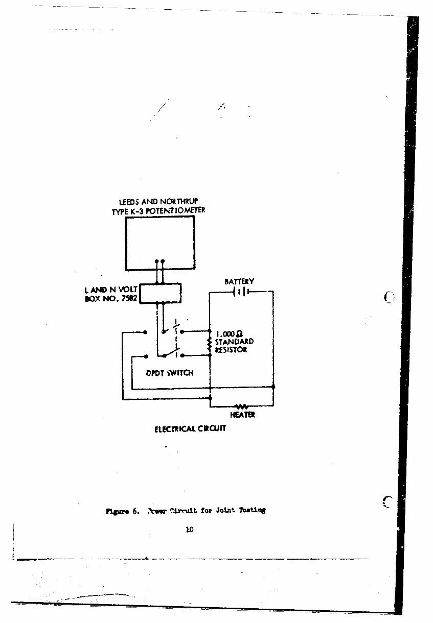
6. Power Circuit for Joint Testing ........ . . . . . . 10

7. Tpical Structural Joint ................... 16

8. Computer Program Flow Mart. . . . . . . . . ... ... .. 33-35

9. Program Input Format . . . . . . . . . . . ... ... .. . 37

1U. Load Sheet for Twm 2'rallel Infinite Diff,jseStrips of Unit Width and Separtion . . . . . ....... 39

U. Load Shoot for Saple Probleim; Diffus1 Aasumption. ...... 41

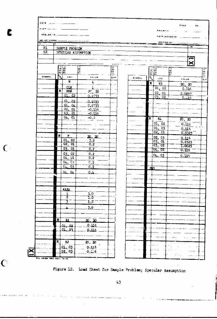
12. load Sheet for Sample Proble; Specular Asmption . .... 3

13. Load Sheet for Saple Prblem; Directional Specular-Diffuse Ausumption . . . . . . . . . . . . . . .. .* . . . . 45

14. Cofiguration Used o Tt of Radiation AiuOasi . . . ... 47

15. Test Coni~iuation !u Toot Fixture . .. .. .. .. .. . .. 48

16. Tuet Oonfgration Rewl7 for Twtin . .. . .. .9 9

17. a tr i f;r Test of RAdiation Amalyis . . . . . . 51

18. Urptional R~leet e oi -AX Flat 0 PSt to .WR B2& 3 as a Puwtim a: Angle .. .. .. .. . .. . 5

19. Z~fttiOiM1 Riftcto of Tau=w repositod Alad.m to a 5400 RMAO& A~s a nMtion of Arng1.... . .... 54

20. 1zwtam Reflw2tawo of &Mliwic Soft. &l, 1.,mTne 100) * 005 bnhos 1ThL to a asr 8oaa Funtion of al. . .. .. .. .. . ........ . 55

3i

//

7 01

" ., "'-.

ILLUS TATI0NS

FIGURE PAGE

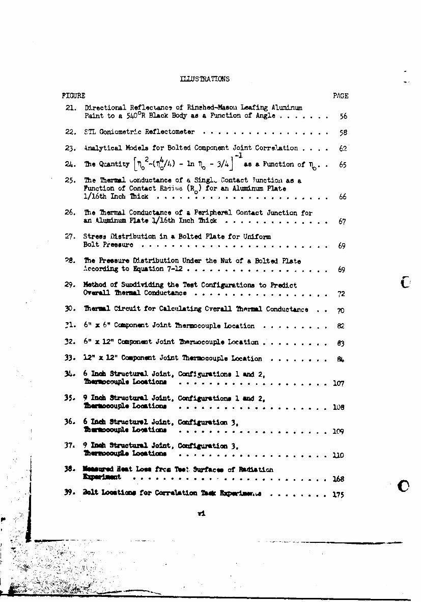
21. Directional Reflectancq of Rinehed-Maaon Leafing AluminumPaint to a 540OR Black Body as a Function of Angle . ...... 56

22. STL Goniometric Reflectometer . . . ............. 58

23. Analytical Models for Bolted Component Joint Correlation . . . . 62

~~~.- 2_ 4/tt L 2 (1 ) _ in I 3 ]as a F'unction of T,. 65

25. The Zherm.l tonductance of a Singl. kontact Tunction as aFunction of Contact Ra&inu (R0 ) for an Aluminum Plate1/16th Inch Thick . . . . . . . . # . . .......... 66

26. The Thermal Conductance of a Peripheral Contact Junction foran kluminum Plate 1/16th Inch Thick ............ ... .. 67

27. Stress Distribution in a Bolted Plate for UniformBolt Pressure . . . . . . . . . . . .. . .. .......... 69

28. The Pressure Distribution Under the Nut of a Bolted PlateAecordig to Euation 7- . . ................ 69

29. Method of Suodividing the Test Configurations to Predict COverall Thermal Conductance . . . .. . . . .. . .. . ... . 72

30. Thermal Circuit for Calculating Cverall Thrmal Conductance . . 70

31. 6" x 6" Component Joint Thermcouple Location ......... 82

32. 6" x 12" Component Joint Therwocouple Location . . . ... . 83

33. 12" x 12" Component Joint Thero oouple Location .. ........ 8

34. 6 Inwh St¢uctumel Joint. Configurations 1 and 2,' op Loations . . . . . . . . . . .. . 107

35. 9 mob Stratw*e Joint, Configurations 1 and 2,SMMootap1.e Loction ......... ...... . . OS

36. 6 Lb 8tructuro. Joint. Configurtion 3,lhusoop 140atin .. . . .. . . .. . .09

37. 9 ID Strutuz l Joit, Ccfi ,'etiom 3.her ~ ~ .oat . .. .. .. .. .. . .. l

I 38. Nm ed ilBat lamn frcs Teest, Swftcm of btdiatin

39. aOl IocatAs for Cor.ation * W'imW,,. . . . . . . . 175

vip. : - -- -

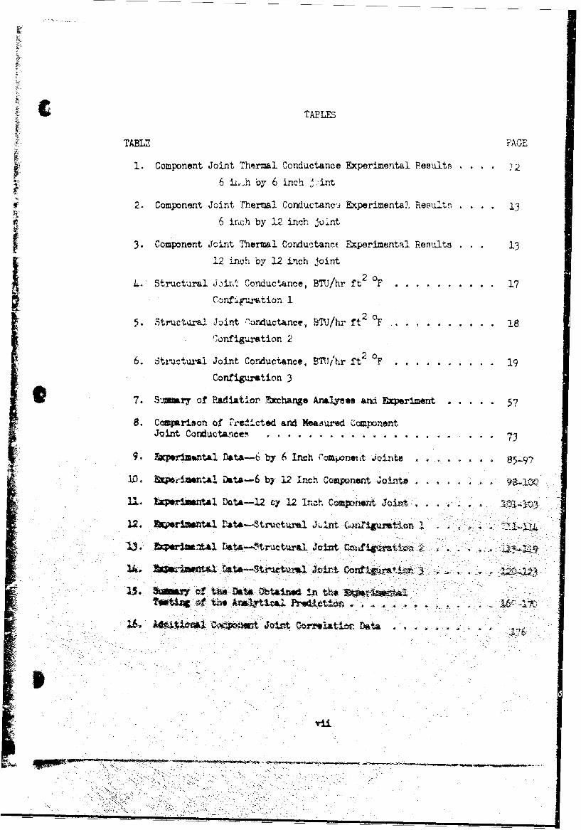
CTABLETABLE PAGE

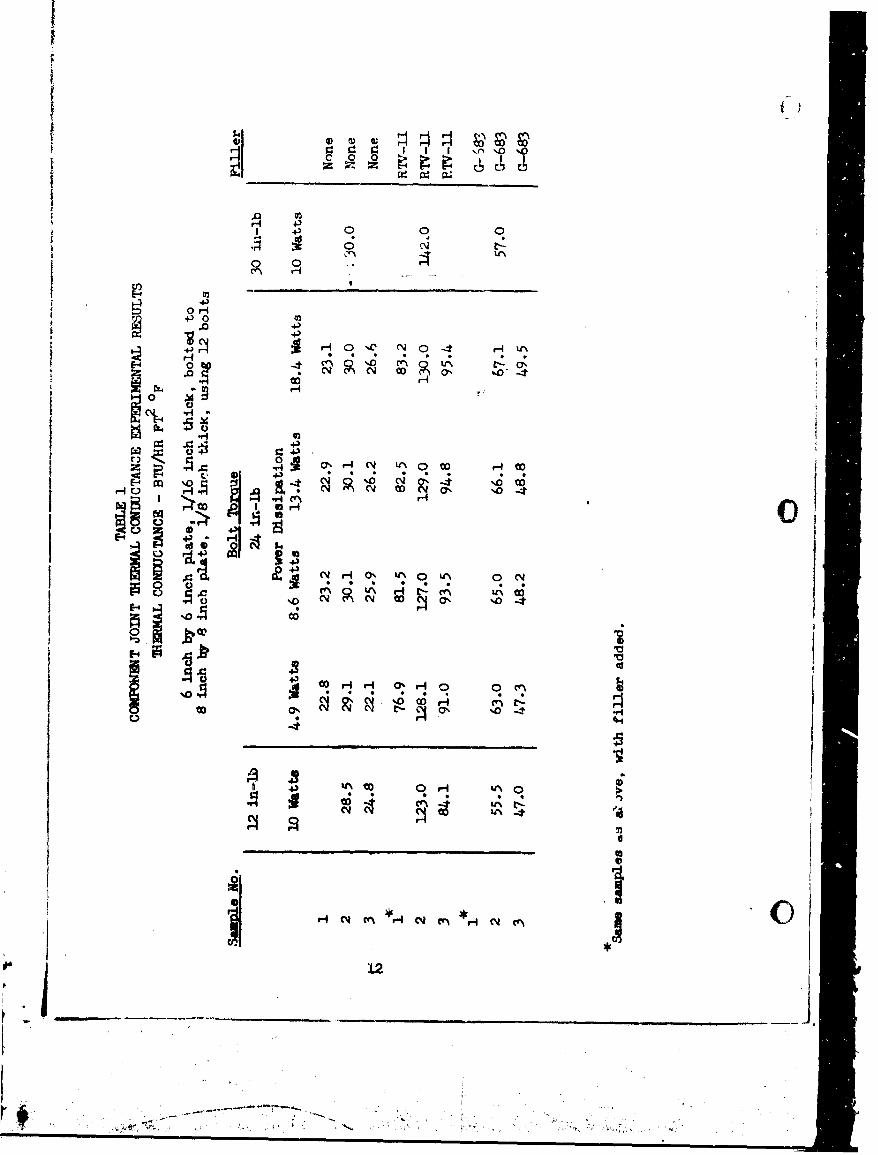
1. Component Joint Thermal Conductance Experimental Results ... .

6 in,,h by 6 inch Jint

2. Component Joint Thermal Conductanc'i Experimental Result . 13

6 inch by 12 inch juKnt

3. Component Joint Thermal Conductance Experimental Results . . . 13

12 inch by 12 inch joint

4.' Stractural Joit Conductance, BTU/hr ft.2 oF ....... ... 17

Confi4uration 1

5. Str ctural Joint "onductance, LTU/hr ft2 OF ..... ......... 18SOnfigurition 2

6. Structu'al Joint Conductance, B"h/hr ft OF . . . . .. . . .. 19

Configurmtion 3

7. S',a.r7 of Radiation Exchange Analyses ad EXperiment •.• .57

S. Csarison of Predicted and Measured ComponentJoint Conductance5. . .. ... ... .. .............. . 73

9. rperiztal Data-6 by 6 Inch roaoneit doiits. ... ... 85-9

!D. b rzi.nntal Dta-6 br 12 Inch Comonent Joints ... ...

U. bqprimtal Data-12 cy 12 Inch Compo nt Jit.....................

12. mj'erintal 1ata-S tueturIint C-4r4t ion 1a.

-13- kpmmtIMM1 tAta-5tractural 'Joint Coinf to02 ,. c,,j

23. Stry af Ubi: Data Obtizd in t-he * maI 70t140. tan" AnlrttoCi Predhttar.- .1 a . .4

It.AG~tiol CtpowtJoint Qnrtit~leta W

.......

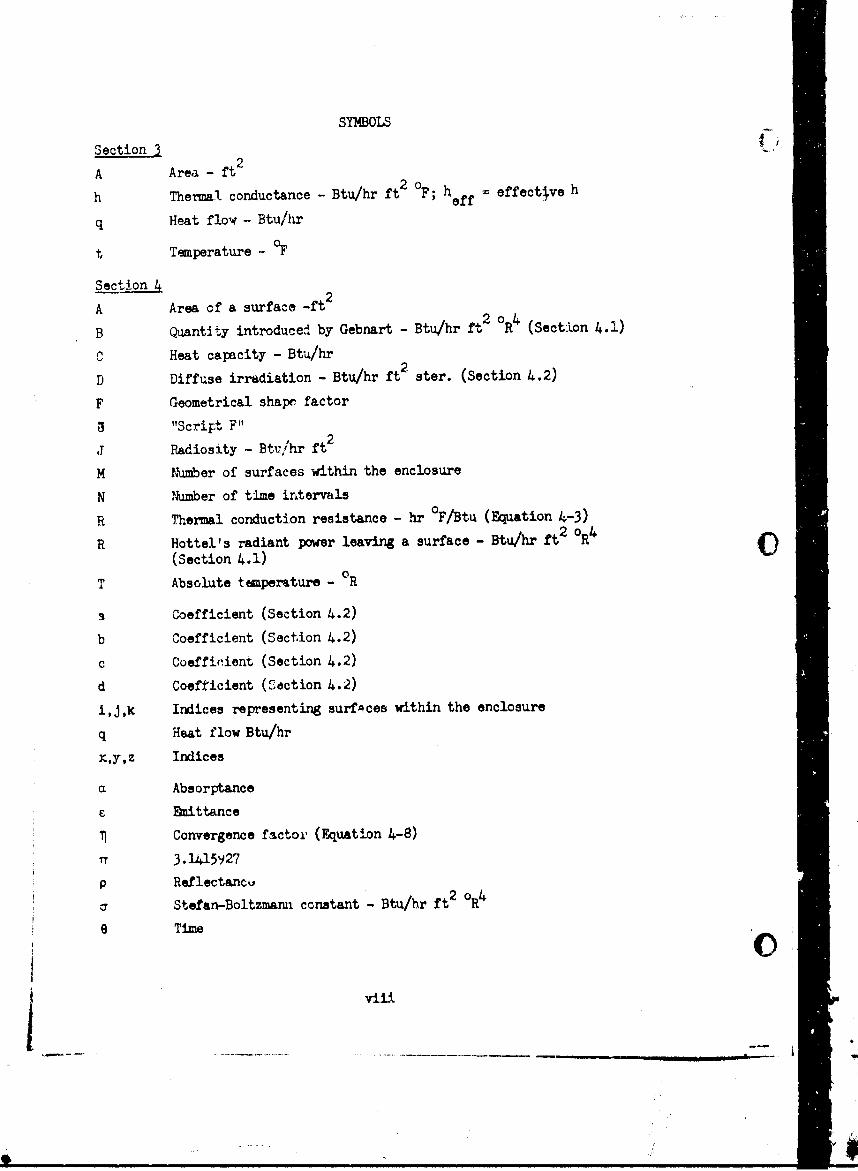
SYMBOLS

Section 3

A Area - ft 2

h Thermal conductance - Btu/hr ft2 OF; h = offectve h

q Heat flow -- Btu/hr

t Temperature - OF

Sect!ion 4

A Area of a surface -ft 2

B Quantity introduced by Gebnart - Btu/hr ft 2 °R4 (Section 4.1)

C Heat capacity - Btu/hr

D Diffuse irradiation - Btu/hr ft2 ster. (Section 4.2)

F Geometrical shape factor3"Script F"

J Radiosity - Btr/hr ft2

M Number of surfaces within the enclosure

N 1umber of time intervils

R Thermal conduction resistance - hr 0F/Btu (Equation 1-3)

R Hottel's radiant power leaving a surface - Btu/hr ft2 OR4

(Section 4.1)

T Absolute temperature - OR

3 Coefficient (Section 4.2)

b Coefficient (Section 4.2)

c Coeffiient (Section 4.2)

d Coefficient (Section 4.2)

i,j ,k Indices representing surfaces within the enclosure

q Heat flow Btu/hr

x,yz Indices

a Absorptance

6Emittance

11Convergence factor, (Fquation 4-8)

I3.1415927

p Reflectancv

a Stefan-Boltzmam constant - Btu/hr ft 2 °Rk

e Time

vi~viii

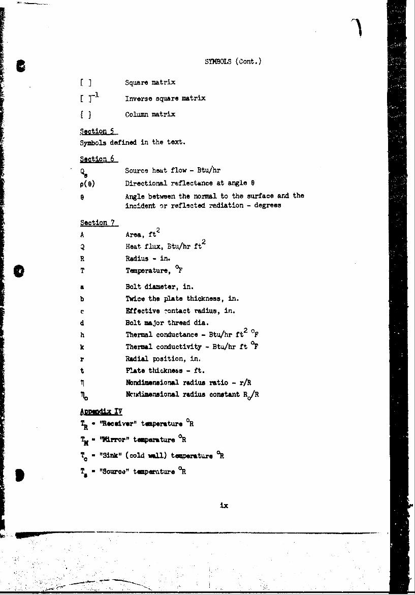
SYMOLS (Cont.)

[ ] Square matrix

Inverse square matrix

L. ] Column matrix

Symbols defined in the text.

Section 6

Qs Source heat flow - Btu/hr

p(G) Directional reflectance at angle 9

0 Angle between the normal to the surface and the

incident or reflected radiation - degrees

Section 7

A Area, ft2

Q Heat flux, Btu/hr ft2

R Radius - in.

T Temperature, OF

a Bolt diameter, in.

b Twice the plate thickness, in.

e Effective ontact radius, in.

d Bolt major thread dia.

h Thermal conductance - Btu/hr ft2 o.

k Thermal conductivity - Btu/hr ft OF

r Radial position, in.

t Plate tic-knebs - ft.

INondimensional radius ratio - r/R

10 Nendiensional radius constant RQ/R

e 'te"eeiver" temperature OR

TX "Mirror" temperature OR

To "Sift" (cold Wal) tomerature OR

T- "Sourc&' temperature OR

ix

1. INTRfODUCTION AND SUM14ARY

The program, "Prediction of Space Vehicle Thermal Performance," wasinitiated on 1 July 1964, under Contract AF 33(615)-1725. The purpose ofthe study can be stated as: Given the necessary analytical methods andexperimeatal data, how well can the thermal performance of a space vehiclebe predicted? The subject program was the first step tow.rds securing ananswer to this question.

The problem provides two natural divisions. The first is theexamination of the analytical procedures needed and the e4)erimental infor-mation required for analysis. The second is the verification of thepredictions of analysis by a thermal test of a model space vehicle, Aepresent program was intended to satisfy the first need and to proviKce Atransition to the second. Since a model is required to verify analysis,its design will dictate the nature and scope of the experimental studiesperformed to support analysis. In particular, the subsequent constructionof a test model will require the selection of structural and componentjoints in anticipation of the design. Depending upon the type of jointselected and the degree of experiental measurements made, the thermalresistance of the joints can be critical to the experimental verificationof any predictions made. Consequently, it ws necessary at the start ofthe present program to select, in reasonable detail, the model configuration.The experimental mearurements of joint thermal resistance were restrictedto those joints to be used in the model. Only in this manner could the endpurpose of the study, the test of prediction, be achieved within theallocated resources and time.

The specific tasks undertaken in the study were:

(a) Selection of a model for determination of the experimentaljoint thermal conductance measurements

(b) Experimental measurement of component and s' uctural jointthermal conductance

(c) Lumination of the results of the joint thermal conductanceresults to ascertain if a correlation were possible

(d) Comparison of the analytical techniques of Hottel (1),Oebhart (2), and Oppenhein (3).

(e) Development of a compter progrm for a specular-diffuse

(f) Experimental measuremnt of radiation exchange with realsurfaces

The following report will consitter the above tasks in the order shown.It should be re-emphasized that the purpose of the program ard hence,the goal of each task, is to provide the necessary data for a compjrisonof theral analysis and thermal test )f a spacecraft model.

1

2. SPACECRAFT MODEL SLECTION

An important initial tank was the conceptual design of the model ofthe space vehicle to be tested in the subsequent phse of the program.The size, method of construction and shape of the mc "el greatly affectsthe type of fasteners, the physical dimensions and the shape of the joints.

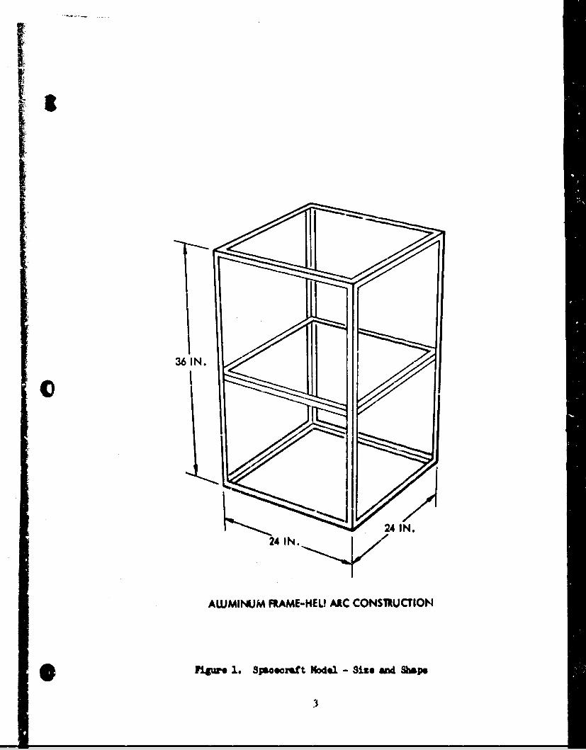
The model which has been selected is shown in Figure 1. Alternativeshapes, cylindrical and spherical, were considered but the rectangularparallelepiped was chosen for economy and ease of fabrication. Further-more, the geometrical shape can not be a critical factor in a test ofthe prediction of thermal performance. The indicated dimensions,24" x 24" x 36", are sufficiently large to demonstrate the effects ofconstruction variations, thermal gradients, and internal dissipation.The model will conveniently fit into most environmental test chambers andavailable solar simulation facilities. Also, the size is representativeof many present day space vehicles.

A welded framework is indicated. This method of construction wasselected to reduce the number of structural joints that had to be tested.There are three stractural joints with the frame: the side panels, theend panels, and the componsit mounting platform, The side and end panelsare 1/16-inch aluminum; i.e., thin enough to sustain a thermal gradient.The mounting platform is 1/8-inch aluminum. In actual space vehicleconstruction, this mounting plate would probably be a honeycomb structureto reduce weight. Such materials are anisotropio and the thermalconductance in the x, y, and z directions are vari able from sample tosample of the same material. The conductance also varies widely fordifferent types of honeycomb. Thus, use of a honeycomb structure wouLdintroduce a major undetermined factor in the thermal analysis. Thiscould easily obscure the validity of the comparison of prediction aniexperiment. The aluminm mounting plate avoids this without affecting thevalue of the teet to be conducted. Thus, if the analysis can properlypredict for the aluminum plate, it will be satisfactory for application toa honeyocb material (aseuming the properties of the honeycomb are known).

The external panels can be changed to provide different externalthermal radiation properties. This my not be important in the initdialteeting to be performed with the model but will be useful should furthertesting be desired or required. These panels can be coated to similatesolar cell thermal radiation properties, low L/c properties or even beinsulted without affecting the basic model O iyscally. A louver systemcould be used in place of any panel to determine the effects of variableemission. Hence, the model will be of much more value than just forthe progmam ontemlated in Phase II.

j,2

36 IN.

IN

24 IN.

AWMINUM FRAME-HELI ARC CONSAUCTION

Pig.. 1. S;S.ocmft Modiel - Size and Sape

3

3. T MAL CMDUCTANCE OF JOINTS

Completely riveted joints were excluded from the study. In spacecraftpractice, riveted systems are used in order to save weight. Howeve;-, thethermal conductance of such joints is not cowsidereda reproducible andvariations of 100 percent have been found in supposedly identical joints (5).Since the goal of the program is to test the ability to predict thermalperformance with reliable input information, the introduction of such anuncontrolled thermal resistance .a not desired. This would not test theprediction of thermal performance but only the uncertainty of knowledge.The effect of the variable thermal resistance canx be demonstrated ana-lytically, once the analysis has been verified.

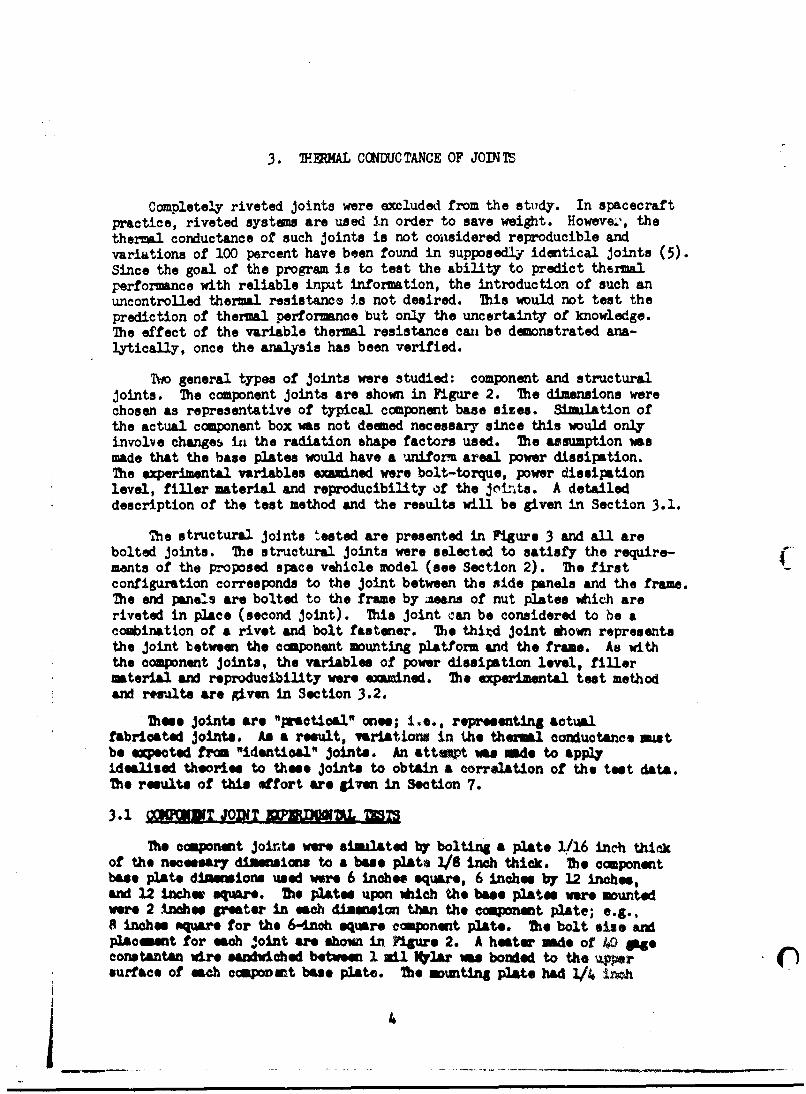
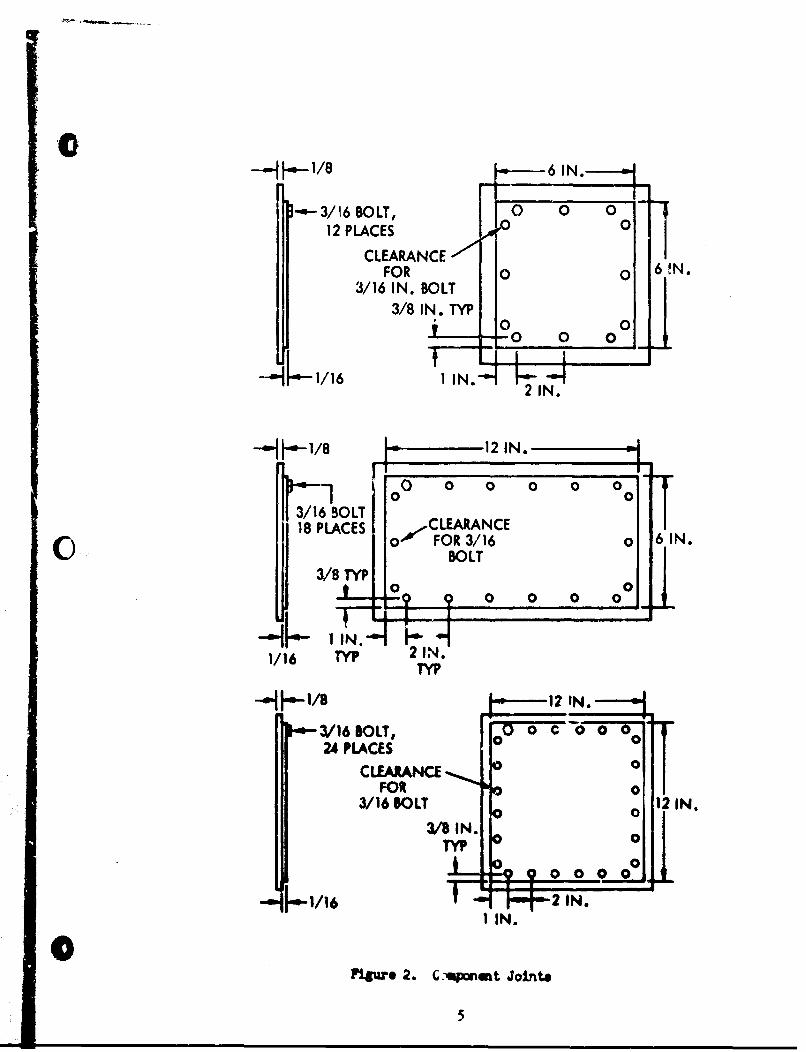
Two general types of joints were studied: component and structuraljoints. The component joints are shown in Figure 2. The dimensions werechosen as representative of typical component base sizes. Simulation ofthe actual component box was not deemed necessary since this would onlyinvolve changes in the radiation shape factors used. The assumption wasmade that the base plates would have a aniform areal power dissipation.The experimental variables examined were bolt-torque, power dissipationlevel, filler material and reproducibility of the jotnts. A detaileddescription of the test method and the results will be given in Section 3.1.

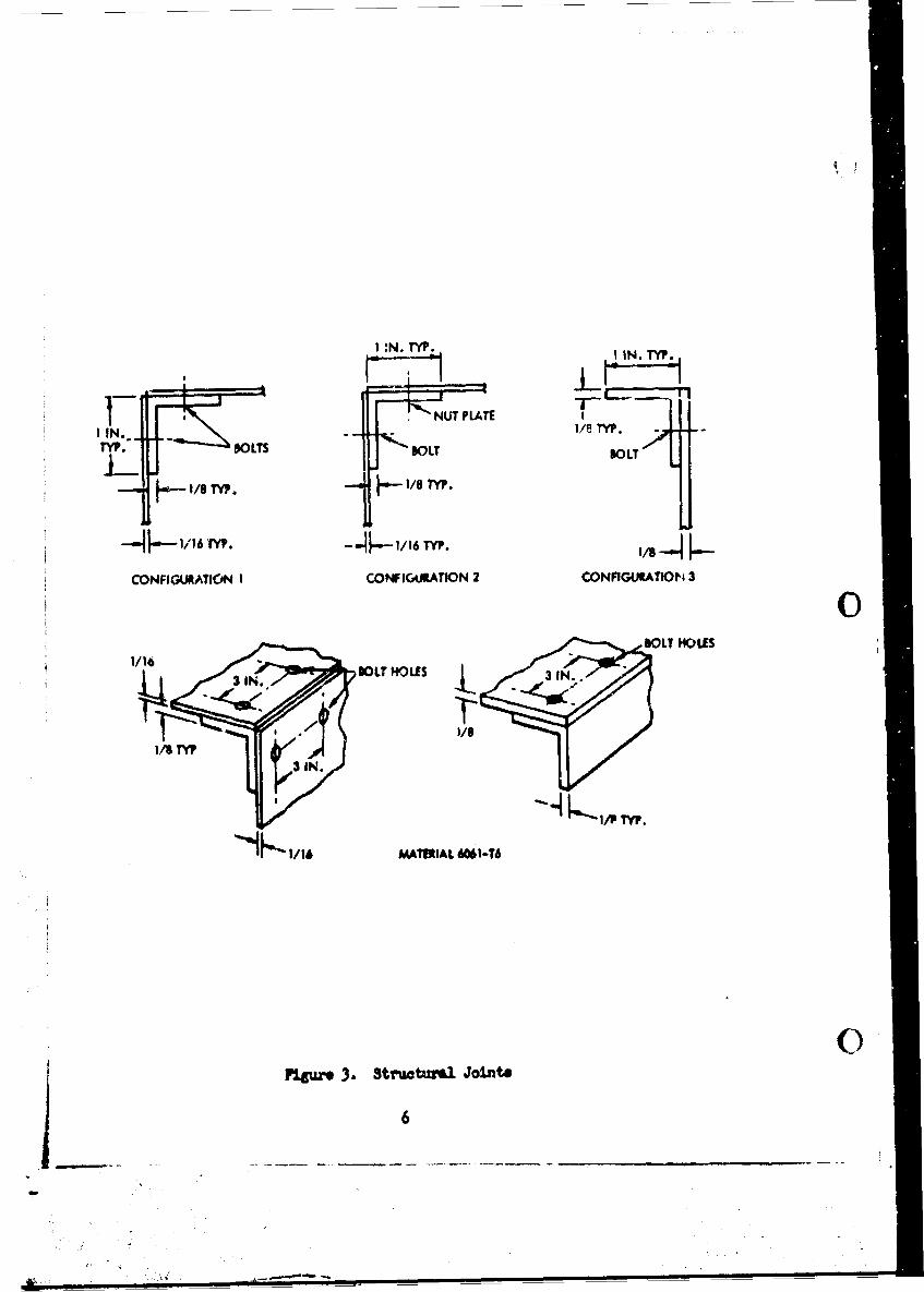
The structural joints tested are presented in Figure 3 and all arebolted joints. The structural joints were selected to satisfy the require- 4mants of the proposed space vehicle rodel (see Section 2). The firstconfiguration corresponds to the joint between the side panels and the frame.The end panels are bolted to the frame by Aeans of nut plates which areriveted in place (second joint). This Joint can be considered to be acombination of a rivet and bolt fastener. The third joint shown representsthe joint between the component mounting platform and the frame. As withthe component joints, the variables of power dissipation level, fillermaterial and reproducibility were examined. The exeimental test methodand resulta are given in Section 3.2.

These joints are "practical" ones; Leo, representing actualfabricated joints. As a result, variations in the thermal conductance nutbe expected from "identical" joint.. An attarpt we made to applyidealised theories to these joints to obtain a correlation of the test data.The result. of this effort are given in Section 7.

3.1 MC3M T JOIRT MMMM3& MM

The component joints we simulated by bolting a plate 1/16 inch thickof the necessary dimensions to a base plate 1/8 inch thick. The componentbase plate dimensions used were 6 inches square, 6 inches by 12 inches,and 12 inches, e are. The plates upon which the base plates were mountedwere 2 Inches greater in each dimension than the component plate; e.g.,8 inches xqure for the 6-inch square component plate. The bolt sise andpiacement for each joint are shown in Figure 2. A heater made of 40 Vgeconstantan wire sandwiched betwen 1 mi1 Iqlar m bonded to the Vpersurface of each conponent base plate. The mounting plate had 1/4 jr'zh

4 - s - - _______________

-- -- /8--6 IN .- 1

3/16 BOLT, 0 0 012 PLACES I ,O0

CLEARANCE 6FOR 0 O 60 N

3/16 IN. BOLT

3/8 IN. TYP0 0

0 0 0

u2NIN

10 0 0 0 003/16 SOLT -,LAAC

--- C o-'-FOR 3/16 0 6 IN.BOLT0

18 P 00 0

4I IN.1/16 FYP T61

1/8 12 IN.

3/16 DOLT, 0 0C 024 PLACES0

CLEARANCE*. 0

FORa3/16 BOLT

1/163,/8 IN 0

TYP

1/16 -HRo okaz- IN.,

I IN.

Figure 2. Gmvponet Joints

5

1 N.TIYN. .p

1- ~ ~ NUT PLATE 18TP

Typ. SOLTS K)OLT SOLT

CONFIOCAAMC*I CONFICAATION 2 CONFIGUATIONr 3

1/16

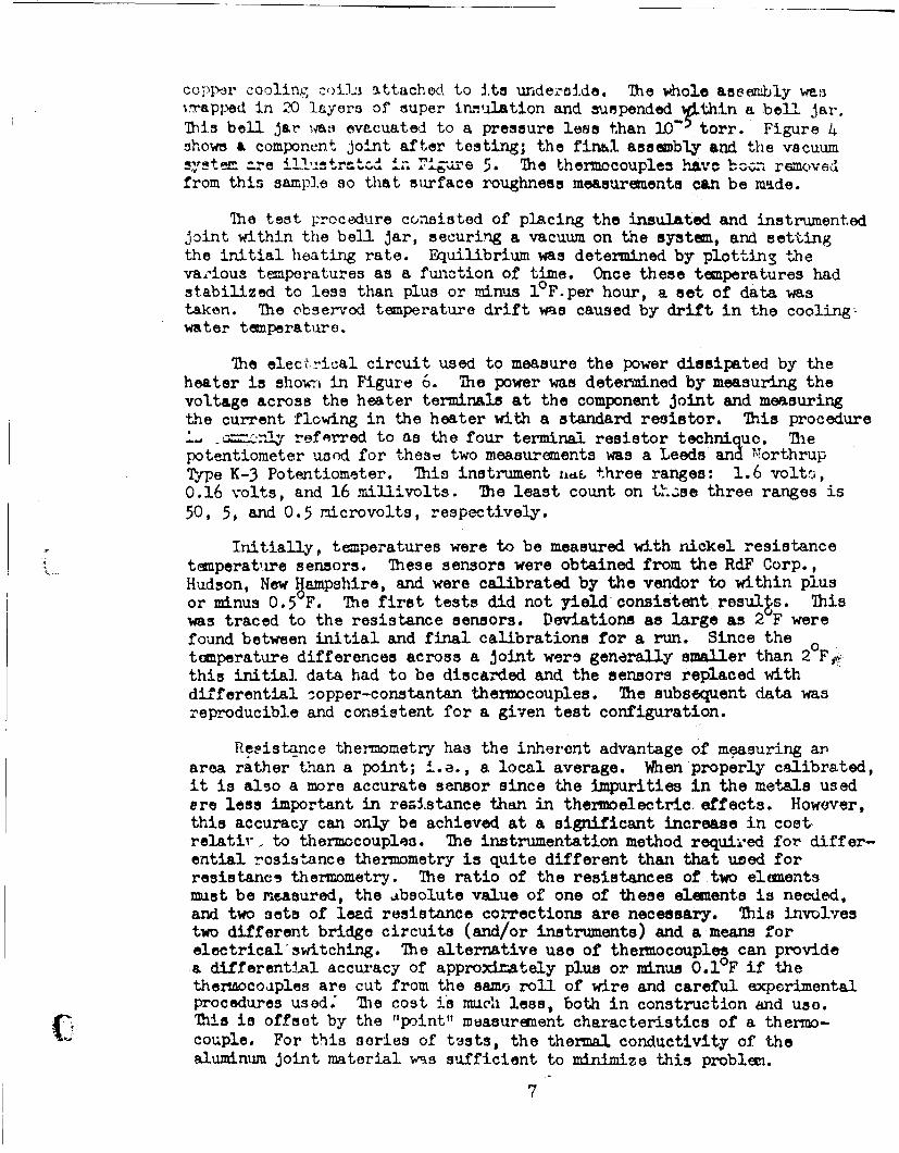
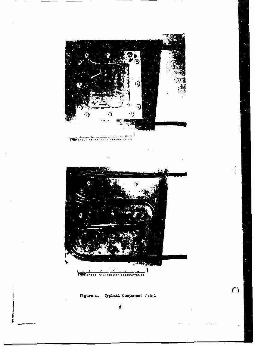
copper cooling coil-j3 96ttached to its underside. The whole assembly wasvrapped in 20 layers of super in.mnlation and suspended m;Lthin a bell Jar.This bell Jar wa3 ovacuated to a pressure less than 10-5 torr. Figure 4shows & component joint after testing; the final assembly and the vacuum3,stem zre__. M tratcd i- "igurae 5. The thermocouples havc boz removedfrom this sample so that surface roughness measurements can be made.

The test procedure consisted of placing the insulated and instrumentedjoint within the bell Jar, securing a vacuum on the system, and settingthe initial heating rate. Equilibrium was determined by plotting thevaroious temperatures as a function of time. Once these temperatures hadstabilized to less than plus or minus l°F.per hour, a set of data wastaken. The observed temperature drift was caused by drift in the cooling,water temperature.

The electrical circuit used to measure the power dissipated by theheater is shon in Figure 6. The power was determined by measuring thevoltage across the heater terminals at the component joint and measuringthe current flowing in the heater with a standard resistor. This procedure', _o='_ rIy referred to as the four terminal resistor techniquc. Thepotentiometer used for these two measurements was a Leeds and 1,'orthrupType K-3 Potentiometer. This instrument atE three ranges: 1.6 volts;,0.16 volts, and 16 millivolts. The least count on those three ranges is50, 5, and 0.5 microvolts, respectively.

Initially, temperatures were to be measured with nickel resistancetemperatLre sensors. These sensors were obtained from the RdF Corp.,Hudson, New gampshire, and were calibrated by the vendor to within plusor minus 0.5 F. The first tests did not yield consistent results. Thiswas traced to the resistance sensors. Deviations as large as 2 F werefound between initial and final calibrations for a run. Since thetemperature differences across a joint were generally smaller than 2°Fe,this initial data had to be discarded and the sensors replaced withdifferential sopper-constantan thermocouples. The subsequent data wasreproducible and consistent for a given test configuration.

Resistance thermometry has the inherent advantage of measuring anarea rather than a point; i.e., a local average. When properly calibrated,it is also a more accurate sensor since the impurities in the metals usedere less important in resistance than in thermoelectric effects. However,this accuracy can only be achieved at a significant increase in cost-relatir, to thermocouples. The instrumentation method required for differ-ential rosistance thermometry is quite different than that used forresistanc thermometry. The ratio of the resistances of two elementsmust be measured, the absolute value of one of these elements is needed,and two sets of lead resistance corrections are necessary. This involvestwo different bridge circuits (and/or instruments) and a means forelectrical switching. The alternative use of thermocouples can providea differential accuracy of approximately plus or mirras O.1 0 F if thethermocoaples are cut from the same roll of wire and careful experimentalprocedures used. The cost is much less, both in construction and use.This is offset by the "point" measurement characteristics of a thermo-couple. For this series of tests, the thermal conductivity of thealuminum joint material was sufficient to minimize this problem.

7

I Figure 4. Thcal Caponent J~int.

8

cii

Fig-,re 5. Component Jain Ready for Iviting

LEEDS AND NORTHRUPTYPE K-3 POTENTIOMETER

BATTERYLAND NVOT -90X NO. 7582

KI STANDARDRESISTOR

I PDT IWTCH

HEATE

ELEC AL CROIT

Flgwe 6. ? Ciruit for Joint Tooting

1.o

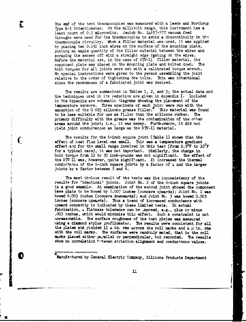
The emf of the test theiiocouples was measured with a Leeds and NorthrupType K-3 Potentiometer. On the millivolt range, this instrument has aleast count of 0.5 microvolts. Deutch No. 14657-37T vacuum feedthroughs were used for the thermocouples to avoid a discontinuity in thothermocouple circuitry. Wheh a filler material was used, it was appliedby placing two 0.050 inch wires on the surface of the mounting plate,putting an ample quantity of the filler material between the wires andscraping the excess off with a straight edge r9sting on the wires.Before the material set, in the case of RTV-ll filler material, thecomponent plate was placed on the mounting plate and bolted down. Thebolt torques for all joints were set with a calibrated torque wrench.No special instructions were given to the person dssembling the joint

relative to the order of tightening the bolts. This was intentionalsince the randomness of a fabricated joint was desired.

The results are summarized in Tables 1, 2, and 3; the actual data andthe techniques used in its reduction are given in Appendix I. Includedin the Appendix are schematic iiagrams showing the placement of thetemperature sensors. Three specimens of each ;oini were run with theexception of the G 683 silicon3 grease filler. This material was foundto be less suitable for use as filler than the silicone rubber. Theprimary difficulty with the grease was the contamination of the otherareas around the joint; i.e., it was messy. Furthermore, it did notyie.d joint conductances as large as the RTV-ll material.

r The results for the 6-inch square joint (Table 1) shows that theeffect of heat flux level was small. Thin was a temperature gradienteffect a-id for tha small range involved in this test (from 2.50F to 10OFfor a typical case), it was not important. Similarly, the change inbolt torque from 12 to 30 inch-pounds was not significant. The effect ofthe RT Vl was, however, quite signif.cant. It increased the thermalconductence of the 6-inch square Joixts by a factor of 4 and the largerjoints by a factor between 5 and 6.

The most obvious result of the tests was the inconsistency of theresults for "identical" Joints. Joint No. 2 of the 6-inch square jointsis a good example. An examination of the second joint showed the componentbase plate to be bowed by 0.007 inches (concave upwards); Joint No. 1 wasbowed 0.003 inches (concave downwards); and Joint No. 3 was bowed 0.003inches (concave upwards). Thus a trend of increased conductance withupward concavity is indicated by these limited tests. In actualfabrication, i flatness tolerance can be .mposed, e.g., plus or minus.003 inches, which would minimize this effect. Such a constraint is notunreasonable. The surface roughness of the test plates was measuredusing a diamond stylus profilcmeter. The results weie consistent for allthe plates and yielded 11 4 in. rms across the roll marks and 4 P in. rmswith the roll marks. The surfaces were randcizy mated, that is the rollmkrks placed either p..allel or perpendicular, but recorded. he resultsshow no correlation 1 'twsen striation alignment and conductance values.

0Mnufturmd by General Electric Compnr, Silicone Products Department

BlmU

I' ilit___________________________________ i li

'D 'c

4

He! .01 -1 *HIU

0 'i cam g JCCV IO u. O

I0 ~ H..

c , (, 4 r%0 t r4t

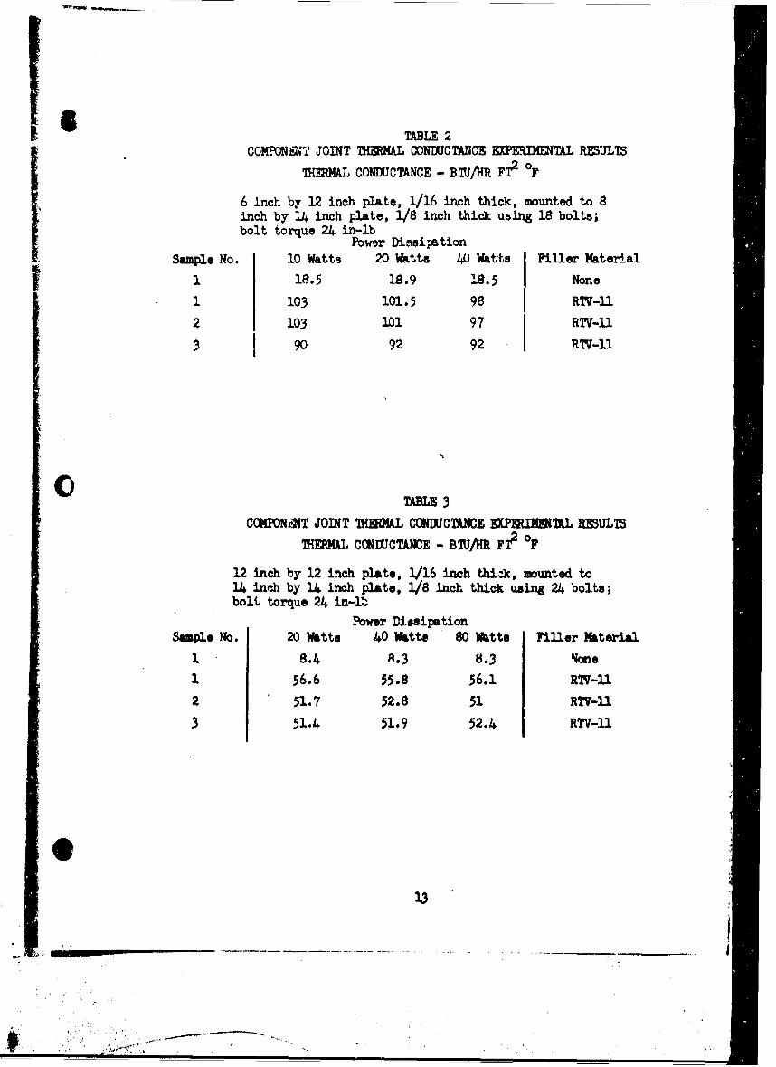
'a TABLE 2CONP!NNvT JOINT TH504AL CONDUCTANCE WEPKUMENTAL RESULTS

T[~MML CONDUJCTANCE - B IU/R Fi' OF

6 Inch by 12 inch plate, 1/16 inch thick, mounted to 8inch by 14 inch plate, 1/8 inch thick using 18 bolts;bolt torque 24 in-lb

Power DissipationSample No.* 10 Watts 20 Watts 40D Watts Filler Material

1 18.5 18.9 18.5 None

1 103 101.5 98 RTV-11

2 103 101 97 RTV-U1

3 90 92 92 RTV-11

C) TABLE 3

CCKPNZNT JOINT TREML C(O4D1CMh.E EXPERI1M411L RESULTS

TMER(AL CC2NI1CTANCE - BIU/HR FT2 OF

12 inch by 12 inch Plate, 1/16 inch thi 1c, mounted to14 inech by 14 inch plate, 1/8 inch thick using 24 bolts;bolt torque 24 in-l

Power DissipationSample No. 20 Watt. 40 Watts 80 Watts Filler Material

1 8.4 8.3 8.3 None1 56.6 55.8 56.1 RWV-11

2 51.7 52.8 51 RTV-ll

3 51.4 51.9 52.4 RTV-fl

33

____________________________________________-_ ---------- ______,

The value of the filler for component mounting boxes is apparent.

For the proposed test of a spacecraft model, the component boxes will besimulated by resistances dissipating pre-determined values of power.This is very similar to an actual spacecraft system. The higher values

of conductance will permit the same heat flow with 1/3 to 14 of thetemperature difference or conversely, 3 to 4 times the heat flow for thesame temperature difference. This should make this type of thermal

resistance less critical in the thermal analysis and prediction.

The effect of using filled joints must be investigated for each

specific application under consideration. While much higher conductancevalues were obtained, the scatter in the data was larger for filledthan unfilled joints. Therefore, the selection of filled or unfilledjoints depends upon whether joints of high conductance, not preciselydefined or joints of low conductance, more accurately described, arelesired.

The differences in conductance for diffMrent sized componentmounting plates was also of interest. The filled conductance decreasedby a factor of 2 when the dimensions of the square component base was

increased from 6 to 12 inches. This decrease is expected since thenumber of bolts doubled while the total area increased four times.1his effectively causes an increase in the conduction pathlength of themounting plate. These factors will be considered in more detail inSection 7, "Correlation of Experimental Results."

The overall accuracy of the tests is difficult to assess properly.However, the experimental accuracy of the various tests quantities canbe given:

Inaccuracy in temperature difference meaeurement: 0 0 F

Inaccuracy in temperature measurement: 0.5 0F

L tccuracy in power dissipation (including insulation loss): _+ .5%

Inaccuracy in area measurement: + .050 in 2

Inaccuracy in bolt torque: 1 0.5 inch-pounds

These values may be combined in a linear error analysis to approximatethe total measurement inaccuracy. That is, the error in measuredconductance (h) of a typical unfilled joint is:

h at q A 1 5

or

Ah- 10. 5%h

The signfiance of this inaccuracy must be appraised in terms of theapplication of the data. The error in the measurement of a single joint

is less than the lack of reproducibility between Joints. Hence, the more

-i 14

C important factor is the variation of the conductance of "identical"joints. As shown in Tables 1, 2, and 3, this is approximately plus orminus 25 percent. However the influence of such a variation upon athermal analysis can be either large or small, depending upon thesystem 'ummine . For example, if a spacecraft thermal control system isconduction controlled, this variation might be critical; conversely, ifit were radiation dominated, the differences might be negligible. Todetermine the importance of these variations requir's an error analysisof the specific configuration.

3.2 STrCMJRAL JOINT EPUINTAL 7ESTS

The test procedures used for the structural joint measurements wereidentical to those used with the component joints. The structuraljoints tested are shown schematically in Figure 3; an actual test jointis shown in Figure 7. A 40 gage constantan and Mylar hoater was bondedto one edge of the joint. On the opposite edge, a.1/4 inch copper coolingtube uas bonded to provide the necessary heat eink. Thit whole assemblywas wrapped in 20 la ers of super insulation and suspended in a bell jar(similar to Figure 5 . The remainder of the test procedure was identicalto that used for the component joints, e.g., the electrical measurementcircuit was that given in Figure 6. Based upon the experience with thecomponent joints, only thermocouples worst used as the temperature sensors.The Ioeds and Northrup Type K-3 Plotentiameter was again used for measuringthe thermocouple voltages.

C TMe test results are given in Wlee 4, 5, and 6; the actual data_

from which these results were reduced are given in Appendix II. Thefirst joint tested, Configrtionl 1 of Figure 3, is representative ofthe trends indicated for all three joints. Within the rane ofpoedissipations used, no dependency upon pow-r Level is indicated forthe unfilled joint; i.e., for small temperature differincee, theconductance is a constant. A much higher value of joint conductancewaobtained with the use of a filler material along with an apparent heatflow dependency. Configuration 2 used nut plate on one side instead ofbolts. his had little effect upon conductance for the unfilled case.Howevor, opposite results were obtained for two different R7V-11 filledjoints with tds configuration; i.e., in one came the rut plate side hada higher conductance and in the other, it had a lever one. Nto differenceobben a bolted joint and a nut Plato joint could be concluded fras theremats for Cnfigmuration I and 2 because of this conflicting data. Astrong dependency7 with heat flow is also noted for the filled joint.

The results of the filled structural joint tests show wide variatipr&in calculated cnductaneo. Te mot probable reason for these vaiAntionois the teMperature nessurent emir. Me temerture diferwe across .the interf'ace me of the MMn order of Magnitudo "s the eaqwted teperstureerror. In ideal joint €onductanesi tests apperin in the literature(see Section 3.3), the tmperatur prfile of the mting part isaceurate1y plotted and the data proj ected to the interface to obtain theteostr difference. The heat flo arenormly nw hi~gher that the

pr~et stad7 and roach Moohr teMperature differcnoee result. In the.

.j15

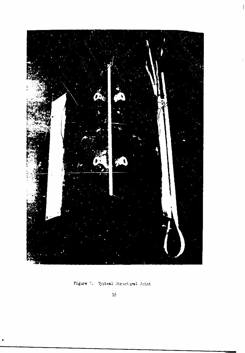
Figure P'. I~a' 3tr IctIral Joint

16

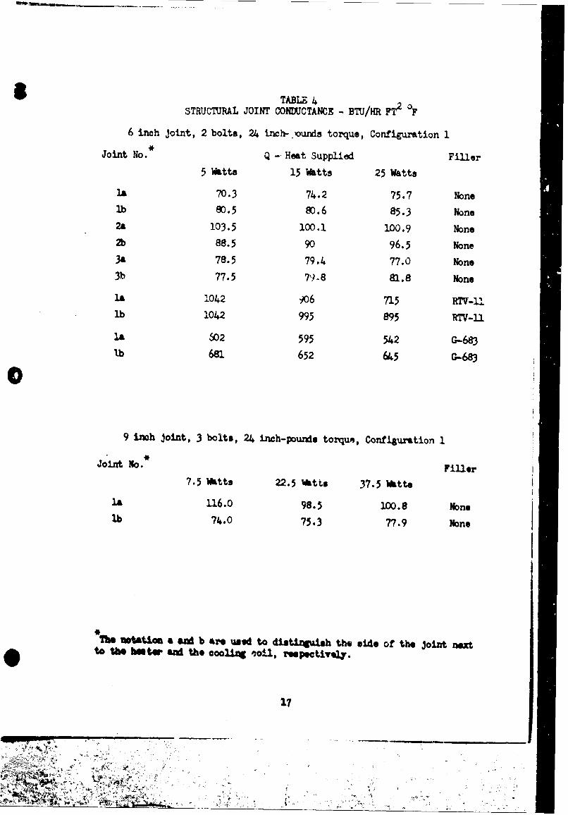
STABLE 4

STRUCTURAL JOINT CONDUCTANCE - BTU/HR FT2 OF

6 inch Joint, 2 bolts, 24 inch- .unds torque, Configuration I

Joint No* Q -Heat Supplied Filler

5 Witte 15 Watts 25 Watts

la 70.3 74.2 75.7 Nonelb 80.5 80.6 85.3 None2a 103.5 100.1 100.9 None

88.5 90 96.5 None3a 78.5 79.4 77.0 None3b 77.5 79.8 81.8 None

la 1042 906 715 RTV-l Ilb 1042 995 895 RTV-u

1. 502 595 542 G-683lb 681 652 645 G-683

9 inch Joint, 3 bolts, 24 inch-pounds torquew, Configuration 1

Joint No. Filler7.5 Watts 22.5 Watts 37.5 Watts

la 116.0 98.5 100.8 Nonelb 74.0 75.3 77.9 lone

*no MUtu a &Mz b are usd to distiogAUh the side of the Joint nextto the hatar w the cooln oil, respectively.

17

77777_

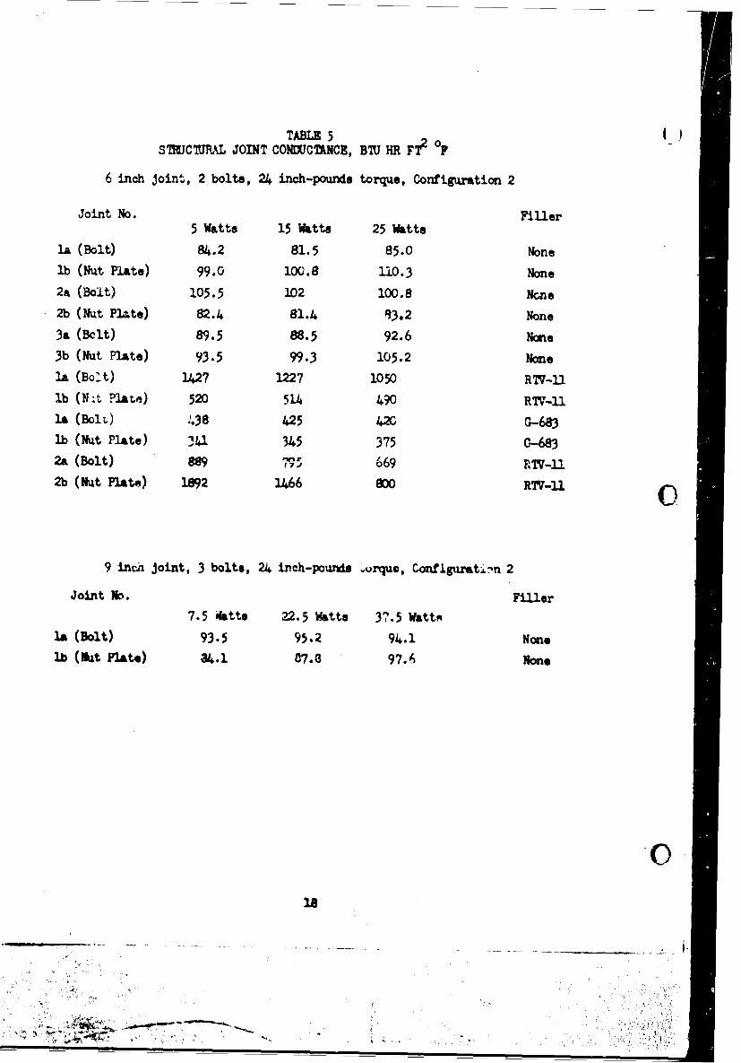
TABLE 54STFJCTUR1 JOINT CONDXCUNCE, BTU HR FT2 OF

6 inch joint, 2 bolts, 24 inch-pounds torque, Configuration 2

Joint No. Filler

5 Watts 15 Watts 25 Watts

la (Bolt) 84.2 81.5 85.0 Nonelb (Nut Plate) 99.0 100.8 110.3 None2a (Bolt) 105.5 102 100.8 None2b (Nut Plate) 82.4 81.4 R3.2 None3a (Bclt) 89.5 88.5 92.6 None3b (Nut Plate) 93.5 99.3 105.2 None

la (Bolt) 1427 1227 1050 RV-U

lb (Nt Plate) 520 514 490 RTV-Ula (Bolt) 438 425 42C G-683lb (Nut Plate) 4I 345 375 0-683

2a (Bolt) 889 075 69 TV-U2b (Nut Plate) 1892 1466 Boo RV-U

9 inch joint, 3 bolts, 24 inch-pounds .Urque, Conflguratimn 2

Joint No. Filler

7.5 iktte 22.5 Watts 37.5 Wattm

14 (Bolt) 93.5 95.2 94.1 Nonelb (Nut PIAte) 34.1 07.0 97.4 Ron*

018I

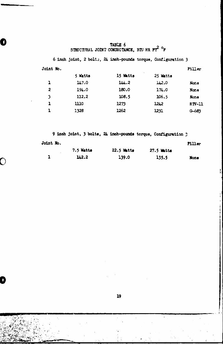
TABIS 6S )CTRAL JOINT CONDTA , BEI HR FTI OF

6 inch joint, 2 bolti, 24 inch-pounds torque, Configuration 3

Joint No. Filler

5 Watts 15 Watts 25 Watts

1 147.0 144.2 142.0 None2 194.0 180.0 174.0 None3 112.2 108.5 106.5 None

1 1110 1273 1242 RTV-111 1328 1262 1231 G-683

9 inch Joint, 3 bolts, 24 inch-pounds torque, Configuration 3

Joint No. Filler

7.5 Watts 22.5 Watts 27.5 Watts

1 142.2 139.0 135.5 None

19

/'Y.

present investigation, the real juints had two dimensional heat fl.o.,. Itwas not possible to project gradient measurements to the interface.Furthermore, the heat fluxes used were selected as representative of those (to be encountered in an actual spacecraft, and the temperature gradieltswere correspondingly small.

Two values of joint conductance are given in able 4 and 5(Configurations 1 and 2) for each test joint. The experimental systemwas instrumented to obtain the -onductance from either plate to theangle. he effective conductance from plate to plate is determined(by analogy to ai electrical circuit) as:

h1heff 1 1

hI h2

If this effective conductanca is computed for "identical" joints andconditions, the variations betweai the measurements are reduced signifi-cantly for the unfillbd joints. In the case of Configuration 1, thevariations in total conductance are less than plus or minus 15 percent;for Configuration 2, it is less than plus or minus 7.5 percent. Thefilled joints have a much wider variation as is indicated by the measure-ments.

Nwo lengths of joint were tested for all three configurations. Nosignificant differences in the mea,ured conductancee were observed. Hence,the end losses from the test joint are considered to have been negligible.

The third configuration tested was the one to be used for conne-ting theinternal mounting plate to the frame. The measured results were similarto those obtained for the other two configurations.

The test resulta obtained indicate a filled structural Joint to bemore variable than an unfilled one. The c-'nduct.nce is aignificantlyhigher, of course. This variability may be nullified by the higher valueobtained. As discussed in Section 3.1, this can on/ y be aisessid byperforning an analysis of an actual spacecraft eyite using these ,p saingconditions. The choice will depend upon the relative importance of the twomodes of heat transfer, radiation and conduction, for the joint asml yz'4and the partievlar system used. However, if filled joints are used, ,formerly conduction dominated system may be-ome radiation controlled. Fore.Mae, the tot). effective conductance of ar unfilled joint is of theorder of 40 to 50 Bt r t OF ere as an RIV-1. filled joint has aconductance of over 500 Btu/hr ft' oF.

0

4. DEgVEOPIMET OF ANALTTICAL n7IThODS FOR IHMAL PMFO CE ANALYSIS

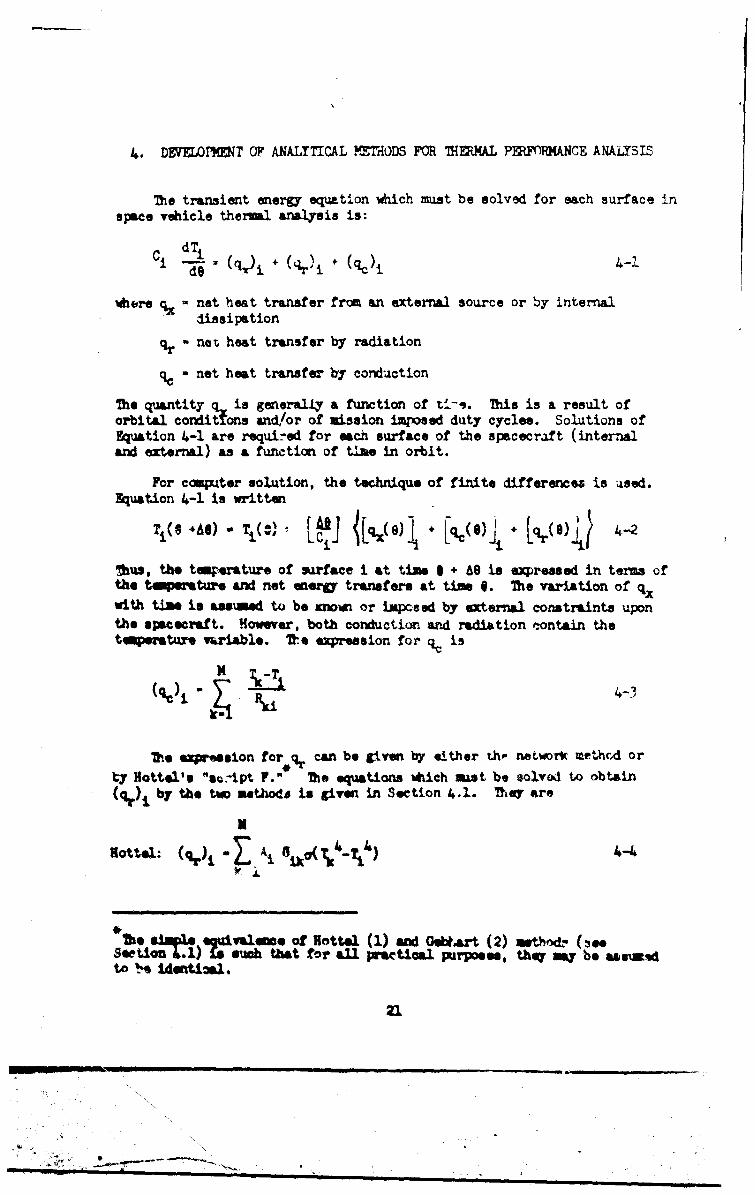
The transient energy equation -wich must be solved for each surface inspace vehicle thermal analysis is:

Ci dTiSd--O = ir.i + (%) * % J

mhere a net heat transfer from an external source or by internal

dissipation

qr - ne heat transfer by radiation

qc - net heat transfer by conduction

The quantity q is generally a function of ti-n. This is a result oforbital condaitons and/or of mission imposed duty cycles. Solutions ofEquation 4-1 are required for each surface of the spacecraft (internaland external) as a function of time in orbit.

For compter solution, the technique of finite differences is used.Equation 4-1 is written

T(s *A@) - r (-&' [i f~ ~ (~ [At]~*~q1 (~j

thus, the tmperature of surface i at time I + 6 is expressed in terus ofthe tnerature and net energy transfers at time 0. The variation of q.with tim is aseuxed to be stn or imposed by external constraints uponthe spacecraft. However, both conduction and radiation contain thetvperatau variable. Ve expression for qc is

M T -T

i - Rki

The expession for q_ can be given by either th- netwrV method or

ty Hottel's "e.Apt F." The equations *tich mast be solvod to obtain(qr)i by the tw methods is given in Section 4.1. 7he are

de la .,.e4 of Hott.3 (1) NWd O*IArt (2) wtMhd,- (0e9eetie U) sueh that for all pmactioel purpoes, they my be a e *dto se 1denti~g1.

21

_ . 'lZ _ I"Ii III -- -".. . . e. _ I ] ,

Networic: (c~r)i = Ai ( IA)j (FJi,Tj) -

M

J 1 + Z F Jk 4k=l

or M

(r)i = AicijTi-Ej 1 Fik Jk 4-7

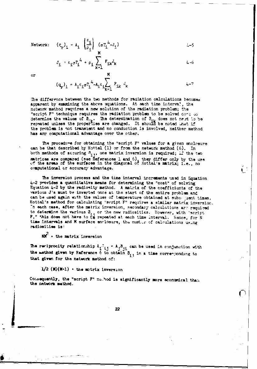
The difference between the two methods for radiation calculations becomedapparent by exmining the abcve equations. At each time interva', thenetwor& method reqires a new solution of the radiation problem; the"script F" technique requires the radiation problem to be solved on-z uO

ietermine the values of a The determination of 5 does not ne-d 'o berepeated unless the properties are changed. It shoul be noted .4,t if

the problem is not transient and no conduction is involved, neither methodhas any coputational advantage ovor the other.

The procedu'e for obtaining the "iscript F" values for a given enclosurecan be that described by Hot tel (1) or from the network method (6). Inboth methods of sc.uring 'I one matrix inversion is required; iL the twomatrices are compared (seelieferer.ncea 1 and 6) they differ only by the useof the areas of the surfces in the diagoral of Aottol's matrix; i.e., nocrsputational or accuracy advantage.

The inversion process and the time interval Increments ,issd in Lquation4-2 provides a quantitative means for determining the "cost" of solvingEquation 4-2 by the radio-ity method. A matrix of the coefficients of thevarious J's must be inverted once at the start of the entire problm andcan be used again with the values of temperature obtained at sub .ient times.Hottl's method for calculAting "script F" requires a similar matrix inversion.

n each case, after the matrix inversion, secondary calculations arc requiredto determine the vurious D or the new radiositics. However, with "scriptF," t!his does not have to j repeated at each time interval. Hence, for Ntime Intervals and M surface en-losure, thu number of calrulatio5 u.aAradiosities is:

+ the matrix inversion

The riprocitty relationship Aij . A jJi can be used in conjunction withthe method given by Reference 6 to obtain aI, in a time corre- )Dnding to

that given for the network method of:

1/2 (X)(NM.) - the =trix inversion

Co .sequent.ly, the "script F" mu.hod is significantly more econordcal tha.,the networt method.

22

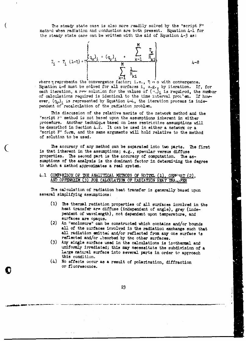
T steady state case is also more readily solved by the "script F"math,-d when radiation and coruction are both present. Equation 4-1 forthe steady state case can be written with the aid of Equation 4-3 as:

Ti t - i-qi ,i + (q) + I

vhere r represents the convergence facto.r; i.e., f o with convergence.Equation 4-8 must be solved for all surfaces i, e.g. by iteration. If, foroach iteration, a rev solutcn for the values of (-ji is required, the numberof calculations required is identical to the time i nterval proL era. If how-ever, (qr)j is represented by Equation 4-4, the iteration process is inde-pendent of recalculation of the radiation problem.

This discussion of the relative merits of the network method and the"script E" method s not based upon the assumptions inherent in eitherprocedure. Another techniqu~e based on less restrictive assumptions Willbe described in Section 4.2. It can be used in either a network or a"script F" furm, and the same arguments will hold relative to the methodof solution to be used.

The accuracy of any method can be separated into two parts. 7he first(is that inherent in the assumptions; e.g., specular versus diffuseproperties. he second part is the accuracy of computation. The as-sumptions of the analysis is the dominant factor in determining the degreeto which a method approximates a real system.

4.1 COMPARISON OF THE ANALYTICAL METHODS OF HOTTrJ (1). G EWRT (2),AND OPPENHEIM (3) FOR CALCULATION OF rADIA iON HEAT TRA,.3FEI

The cal culation of radiation heat transfer is generally based uponseveral simplifying assumptions:

(1) The thermal radiation properties of all surfaces involved in theheat transfdi aro diffuse (independent of angle), grey (inde-pendent of wavelength), not dependent upon temperature, andsurfaces are opaque.

(2) An "enclosure" can be constructed which contains and/or boundsall of the surfaces involved in the radiation exchange such thatall radiation emitted and/or reflected from any one surface tsreflected and/or ,bsorbed by tnc other surfaces.

(3) Arn sirigle surface used in the calculations is isothermal anduniformly irradiated; this may necessitate the subdivision of ala:ge natural surface into several parts in order to approachthis condition.

(4) No effects occur as a result of polarization, diffractionor fljuoreecence.

23

I,

Three different methods of .iewing the solution of this radiation exchange

problem are available. These are generally knrn as the "script F"

method (Hottel), Gebhart's method, ard the network (Oppenheim).

Intuitively, these methods must be identical since they are based upon

the same physical assumptions and the conservation of energy. However,

it is important that this equivalence be demonstrated. Sparrow (7)

has recently shown this by developing the methods of Hottel and Gebhart

from the network method. Since the "script F" method has been advocated

as a more useful approach in complex transient radiation exchange, the

"script F" method will be used here as the method of comparison.

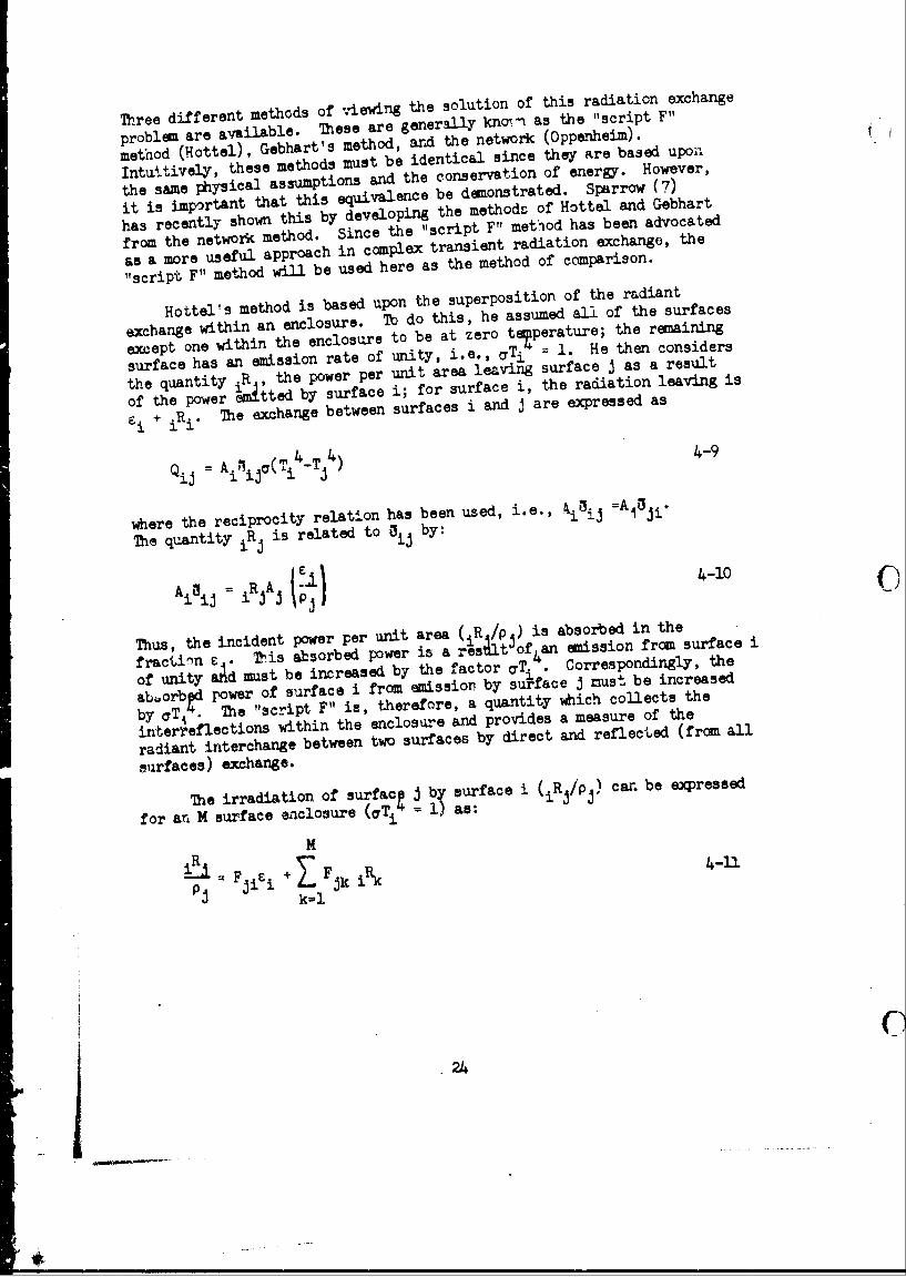
Hottel's method is based upon the superposition of the radiant

exchange within an enclosure. Tb do this, he assumed all of the surfaces

except one within the enclosure to be at zero t lperature; the remaining

surface has an emission rate of unity, i.e., aTi = 1. He then considers

the quantity iR , the power per unit area leaving surface J as a result

of the power Wemtted by surface i; for surface i, the radiation leaving is

6i Ri The exchange between surfaces i and j are expressed as

4_= Ai'4iJa(Ti - Tj") 4-9

where the reciprocity relation has been used, i.e., ij =A3ji"

The quantity iRj is related to OiJ by:

Ai ij iRjAj i-10

Thus, the incident power per unit area (iR /P ) is absorbed in the

fraction e . This absorbed power is a res$lt' of 4 an emission from surface i

of unity a. must be increased by the factor CTi * Correspondingly, the

aborbd power of surface i from emission by surface j must be increased

by aT 4 The "script " is, therefore, a quantity which collects the

inter 4 flections within the enclosure and provides a measure of the

radiant interchange between two surfaces by direct and reflected (from all

surfaces) exchange.

The irradiation of surfact J b surface i (iRi/P ) can be expressed

for an M surface enclosure (aTi 1) as;

M

i_ + F~ j i-ll

24

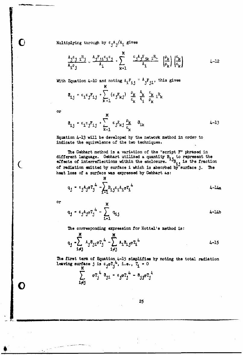
ultiplying tnrough by ejAj/Ai givesM

A~ i CjR j A M A FAii jj 1ij 1 i j j hk i_ [Pk) [5) 4-12

A p A. i-E A LIP 'jj k=1li

With Equation 4-10 and noting A = AjFji, this gives

Cl = jFj + (F-jF ) Pk k E_ akHj jk j -k=l ek Ai Pk

orM

a = F + C k 4-13k=l k

Fquation 4-13 will be developed by the network method in order toindicate the equivalence of the two techniques.

The Gebhart method is a variation of the "script F" phrased indifferent language. Gebhart utilized a quantity B1 4 to represent theeffects of interreflections within the enclosure. - B is the fraction

of radiation emitted by surface i which is absorbed by surface J. Theheat loss of a surface ws expressed by Gebhart &s:

M

qj = .AjcT 4 -BiEiAi7Ti 4-14a

or M

qj o £jAj7Tj- qiJ 4-4b±il

The corresponding expression for Hottel's method is:

H H

qj -Z AjgjiTj4 -Z A1~ijoT14 4-15

i#j i~j

The first term of Equation 4-15 simplifies by noting the total radiation

leaving surface j is EjaTJ4 , i.e., Ti - 0M

O i#j

25

4 n u un nn nm

or

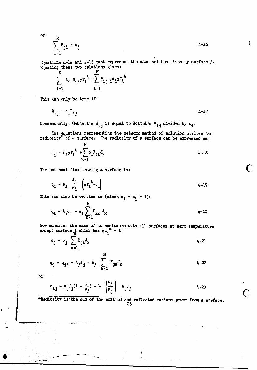
SJi = F4 -16

i=l

Equations 4-14 and 4-15 must represent the same net heat loss by surface j.Equating these two relations gives:

M MZ A i i~c~4 = Z B i jF-iA i cyTi4

i~l i=l

This can only be true if:

Bij- Bi i4-17

Consequently, Gebhart's Bij is equal to Hottel's I iJ divided by Ei.

The .equations representing the network method of solution utilize theradiosity of a surface. The radiosity of a surface can be expressed as:

M

i = SiaTi 4 + PiFikJk 4-18k=l

The net heat flux leaving a surface is: C

% = Ai -1 ,Ti) 4-19

This can also be written as (since ci + Pi = 1):M

qi =AiJi - Ai ik Jk 4-20

Now consider the case of an enclosure with all surfaces at zero temperatureexcept surface i which has aTi= 1.

Fj j FjkJ 4-21

k-l

M

qJ qij o -Aj j A FjkJk -22k=1

or

qjj Ajl(l -- (:) A J 4-23

*Radiosity is the sum of the emitted and reflected radiant power fron a surface.26

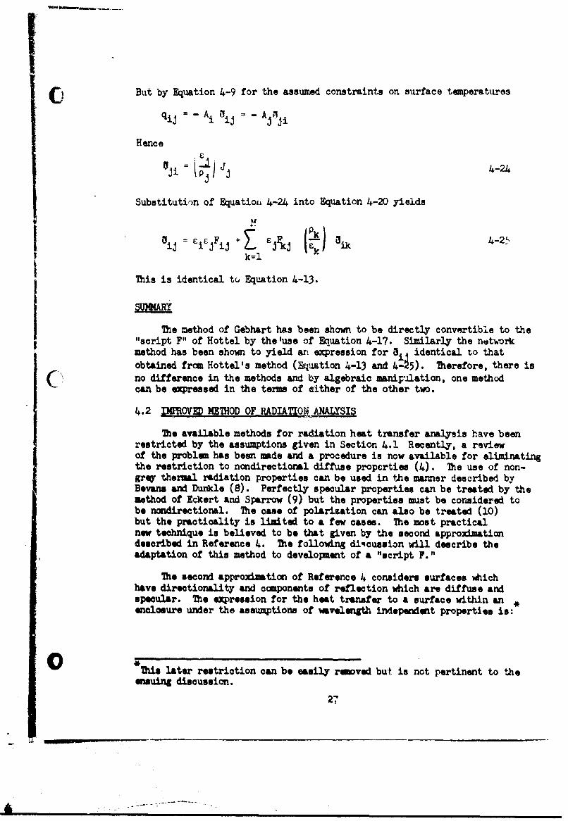
CI But by Equation 4-9 for the assumed constraints on surface temperatures

qiJ A Ai Ai = - I

Hence

ji = I~j# Jj 4-24ji

Substitution of Equatioll 4-24 into Equation 4-20 yields

Fj + __ If 4-25i k=l

This is identical tu Equation 4-13.

The method of Gebhart has been shown to be directly convertible to the"script F" of Hottel by the use of Equation 4-17. Similarly the networkmethod has been shown to yield an expression for i identical to thatobtained from Hottel's method (Equation 4-13 and 4-25). Therefore, there is(I no difference in the methods and by algebraic manipalation, one methodcan be expressed in the terms of either of the other two.

4.2 PWOVI METHOD OF RADIAMON ANALYSIS

The available methods for radiation heat transfer analysis have beenrestricted by the assumptions given in Section 4.1 Recently, a reviewof the problem has been made and a procedure is now available for eliminatingthe restriction to nondirectional diffuse proporties (4). The use of non-gray thermal radiation properties can be used in the manner described byBevana and Duxkle (8). Perfectly specular properties can be treated by themethod of Eckert and Sparrow (9) but the properties must be considered tobe nondirectional. The case of polarization can also be treated (10)but the practicality is limited to a few cases. The most practicalnew technique is believed to be that given by the second approximationdescribed in Reference 4. The following diqcussion will describe theadaptation of this method to development of a "script F."

The second approximation of Reference 4 considers surfaces whichhave directionality and components of reflection which are diffuse andspecular. The expression for the heat transfer to a surface within an *

enclosure under the assumptions of wavelength independent properties is:

* Tis later restriction can be easily removed but is not pertinent to theensuing discussion.

2.

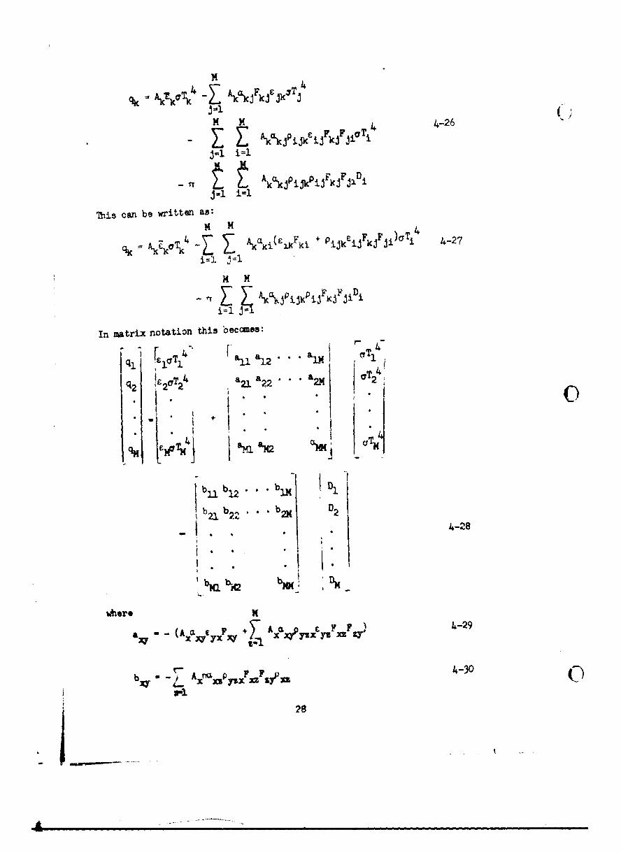
~ 14

j4 14 42

This can be written as:

4 Ti

In matrix notationl this beccfls'

4 ~ rl T14

q, e17T, ll a1

q2 2' 122 2M T

m T Ia* T1

lbil b12. b ix D,

- * *4-28

&V -(A,~ AX%9 73X Ez'x 4-29

b *-r A nr U~ 4-.30

28

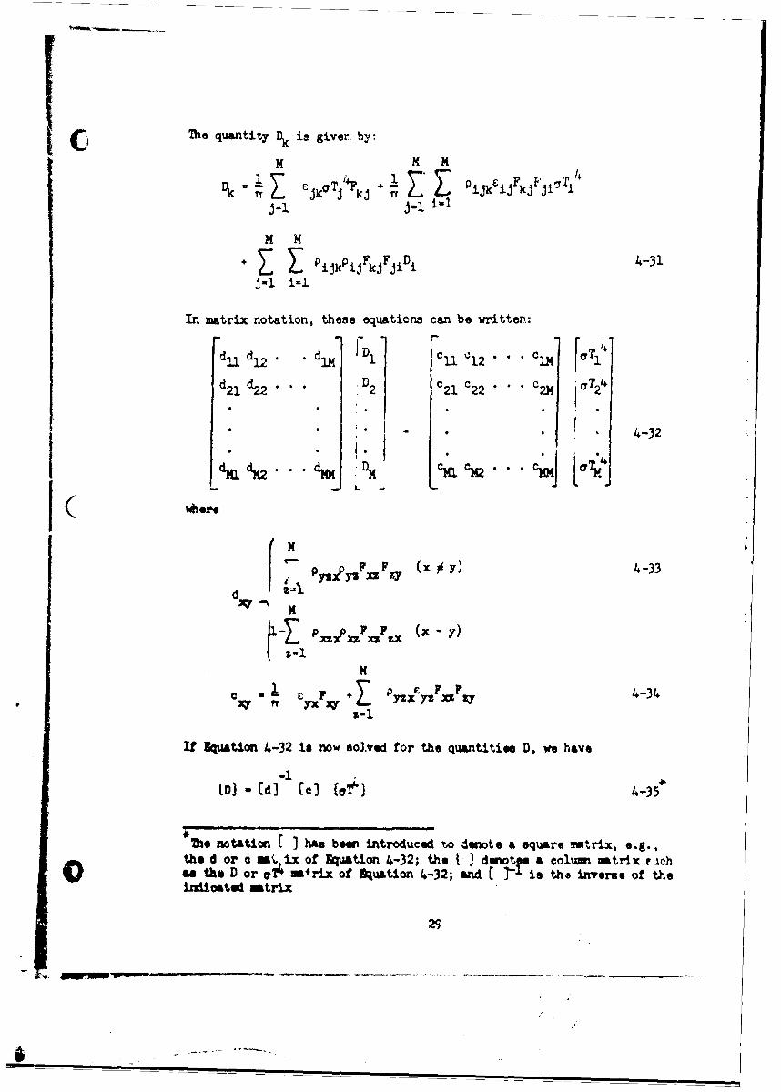
The quantity Dk is given by:

M MM

Dk=a jkTj " PijkcijFkj"J i'k T .1J. i- £

M M

+ Z E Pijkp ijFkjFjiD 4-31

j-1 i-

In matrix notation, these equations can be written:

.~ dl . d' I-. Tdl al2• im '1 'l 12 • * • C'1M L'

d21 d22 * "D 2 c 2 1 c22 * * " c2M aT24

* 4-32

- M

I .•

F F (x y) 4-33

d -1

CcF +3E F F 4-..34S-1

If 3uation 4-32 is now solved for the quantities D, we have

The notation Me ] has bow introduced to denote a square m!trix, e.g.,the d or oa mst. ixof Suation 4-32; the ) 3 dootpe a column matrix rich0a the D or mi? Mrx of Dquation 4-32; er 'C is the inverse of theindicated mtrix

29

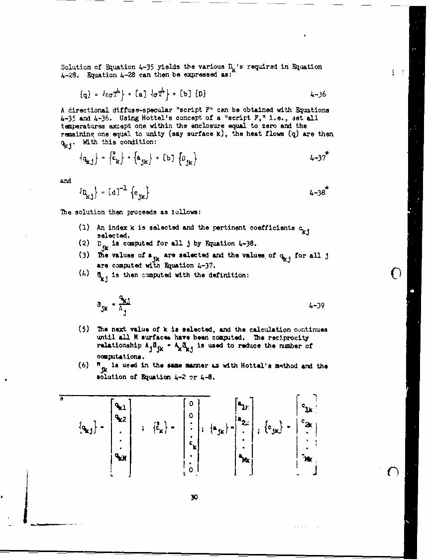
Solution of Equation 4-35 yields the various Dk's required in Equation4-28. Equation 4-28 can then be expressed as:

[q) = 46aT} + [a] laT4} +Eb] [D) 4-j6

A directional diffuse-specular "script F" can be obtained with Equations4-35 and 4-36. Using Hottel's concept of a "script F," i.e., set alltemperatures except one within the enclosure equal to zero and theremaining one equal to unity (say surface k), the heat flows (q) are thenqk" With this condition:

q {J e kJ + {J + [b] 4-37

and

I~kjj [d]-lfcjkl4-38*

The solution then proceeds as tollows:

() An index k is selected and the pertinent coefficients Ckjselected.

(2) Djk is computed for all J by Equation 4-38.

(3) The values of ajk are selected and the values of kj for all jare computed with Equation 4-37.

() j is then c.3mputed with the definition:

k " k 4-39J

(5) The next value of k is selected, and the calculation cuntinuesuntil all N surface. have been computed. The reciprocityrelationship A 3 3k - A is used to reduce the number of

computations.(6) Nk is used in the same maimer &a with Hottel's method and the

solution of Equation 4-2 cr 4-8.

r 1

k20 ja~ic

*11

" I -;B'X

~ .quat8or prosntd i this section ay apper to be mree~~n~~lmgc~ted and hence, more difficult than "0 h ifuepoet

t thMatica&iY, this is not the case. 2ie computations are"gumption. -- ... r- added computer time and storage space._r tiGcr~~r v j o~rQ evct camutations.

(

1031

5. COMPUTE PROGRAM FOR DIREC71ONAL SPEJLAR-DIFFUSE MEJIOD

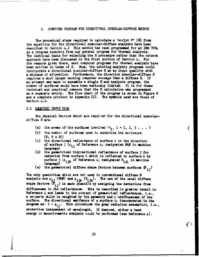
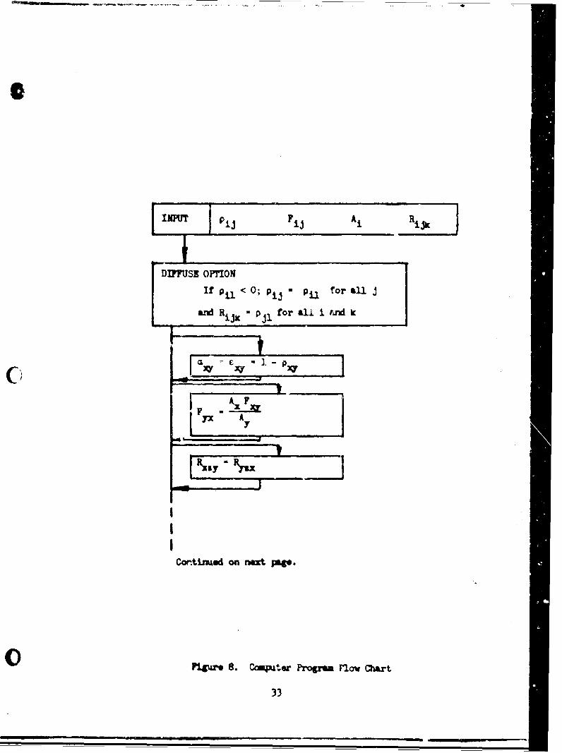
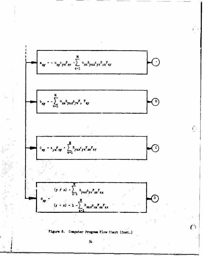
The procedural steps required to calculate a ,script F" (0) fromthe equatJons for the directional specular-diffuse analysis have beendescribed in Section 4.2 This method has been programed for an IBM 7094as a program separate from arq general program for thermal analysis.The technical basis for selecting the 0 procedure rather than the networkapproach have been discussed in the first portion of Section 4. Forthe reasons given there, wst computer programs for thermal analysis havebeen written in terms of . Thus, the existing analysis programs couldincorpurate a directional specular-diffuse a as an input quantity witha minimim of alteration. Furthermore, the direction specular-diffuse arequires a much larger working computer storage than a diffuse 3. Ifan attempt was made to assemble a single 8 and analysis program, thenumber of surfaces would have been seriously limited. It is for theetechnical and practical reasone that the 8 calculation was progreamsdas a separate entity. The flow chart of the program is shown in Figure 8and a complete printout in Appendix III. The symbols used are those ofSection 4.2.

5.1 RJIRN UT DATA

The physical factors which are required for the directional specular-diffuse 0 are:

(a) the areas of' the surfaces involved (A., i - 1, 2,3 . . )(b) the nubier of surfuces used to subdivide the enilosure

(N; N x2)(c) the directional reflectance of surface i in the direction

of surface J (PiJ of Roference 4; deeirated RH in machinelang e)

(d) the geomtrical bidirectional reflectance of surface J forradiation from surface i which is reflected to surface k bysurface i(p of Ref erence 4; designated Ri~j in mactiineunuae)

(e) the geometrical diffuso shape factors between surfaces ij)

The only quantities which are not used in convaltional diffuse eanalysti are p (Rio) and pik (Rij). V.e use of the usual diffuseshape factore tiij) is made possib] by *.ssigr$4 the deviations from

diffuseness to the reflectance@. This is described in greater detail inRefwerece 4 and leads to the concept of geometrical reflectances, i.e.,a prmperty 4.ich is weighted by the geometry and n diffuseneae of thesurface. The directional sttance of a surface iL inorporated in theprogram : I - pi Ti introduces the gr*y radiation asmption, i.e.,

Propertioe indepecdent of wvelrngth. If desired, either a bandenergy or onohr tic analysis could be Perforled (see Reference 4).

32

_____

DIFFUSE OPTIONf

If i., <0; pj - in f~ ora &11

anRi. p = for &UJ i rxnd )c

y

Cortimed on next jg.

0 ?Figu"r 8. C4mpter Prop..m Jlov Chart

33

m

-~~F - ~ ReF~F:4 .P.xxI

V,

R *c F

34

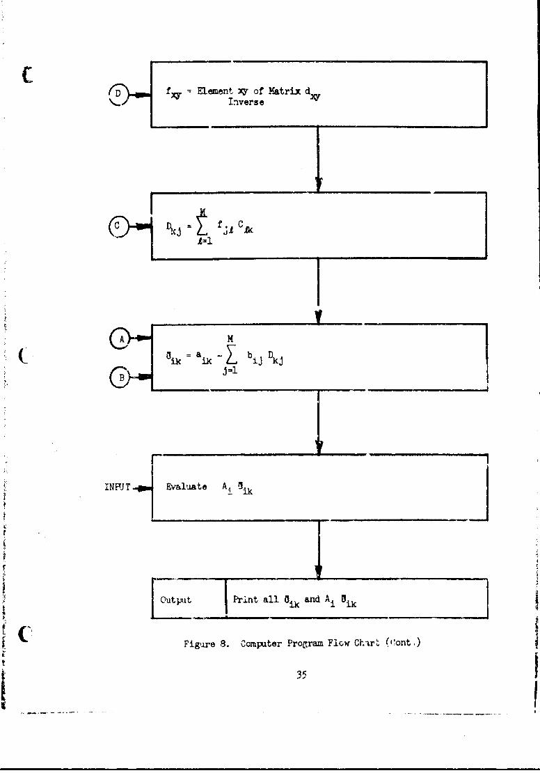
fx D 13 Element -V of Yatrix d,,

Inverse

~Ak

( I ik=&a,, bl. Dkj

INFU T Evaluate Ai Iik

Zupt Print all 0ik and Ai ik

Figure 8. Computer Program Flow Chtrk (',ont,)

35

Values of piJ and piJk (RHO and R ij k ) -an be approximated with data

obtained in many Thermophysics Laboratories (4). The methods suggestedfor this approximation will be illustrated in Section 5.3 and 6.2

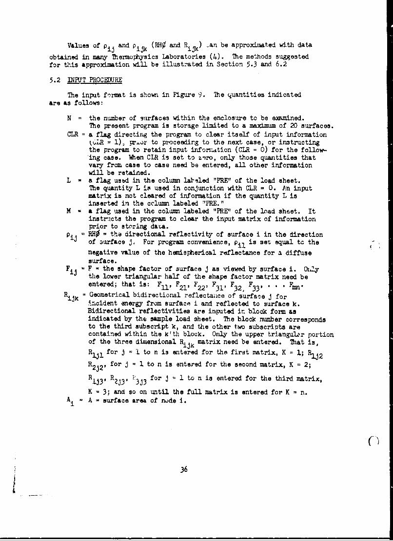
5.2 INRJT PROCEDURE

The input fcrmat is shown in Figure 9. The quantities indicatedare as follows:

N = the number of surfaces within the enclosure to be examined.The present program is storage limited to a maximum of 20 surfaces.

CLR a flag directing the program to clear itself of input informationkULR = 1), prior to proceedirg to the next case, or instructingthe program to retain input informAtion (CLR = 0) for the follow-ing case. Wen CLR is set to z~ro, only those quantities thatvary from case to case need be entered, all other informationwill be retained.

L = a flag used in the column labeled "PRE" of the load sheet.The quantity L is used in conjunction with CLR = 0. An inputmatrix is not cleared of information if the quantity L isinserted in the cclumn labeled "PRE."

M = a flag used in the column labeled "PRE" of the load sheet. Itinstracts the program to clear the input matrix of informationprior to storing data.

PiJ = RHO = the directional reflectivity of surface i in the directionof aurface J. For program convenience, pil is set equal tc thenegative value of the hemispherical reflectance for a diffusesurface.

Fij - F = the shape factor of surface J as viewed by surface i. 04ythe lower triangular half of the shape factor matrix need beentered; that is: Fll, F2 1, F2 2, F31, F3 2 , F3 3 , * .. Fn

Rijk = Geometrical bidirectional reflectance of surface j forincident energy from surface i and reflected to surface k.Bidirectional reflectivities are inputed in block form asindicated by the sample load sheet. The block number correspondsto the third subscript k, and the other two subscripts arecontained within the i' th block. Only the upper triangul.'r portionof the three dimensional Rij k matrix need be entered. Mat is,

Rij I for J I to n is entered for the first matrix, K = 1; RJ2

R2J21 for j = 1 to n is entered for the second matrix, K = 2;

R I 3 R2 J3 "3J3 for j = I to n is entered for the third matrix,

K - 3; and so on until the full matrix is entered for K = n.Ai - A - surface area of nude i.

36

DATE

C IIII~~~~VOBl. a.M NO. .M Y NC D .

NO. OF C AMC$} VERIF~IED .....

l H A ~ E - LIMITED .,n 6 6 ! .JTh M I CE - US M ,

H2 AS RUN DCRIPTION ONLY

| I 0 7 ll I? IaI 4II II I1 9O 20 i

. . . .I V--- . . . . I t 3

4 2RHO 20 I 20 I

01 01[

E V M O L•I O . - A U L . V A U

N

oil

j.- --- - - I -

--" END-* ---

X20, 20....

I I-

1w --- - ------ -- -

__ __ 1 N'2

Figure 9. Program Input Funnat

II 37

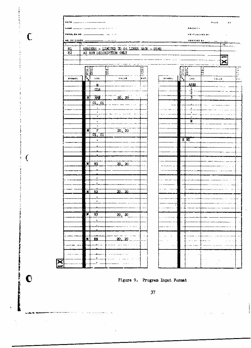
An wlimited number of cases may be "stacked"; all that is requiredto run several cases together is an END card between cases. Outjtquantities 0 and -area products, are printed out in matrix form.

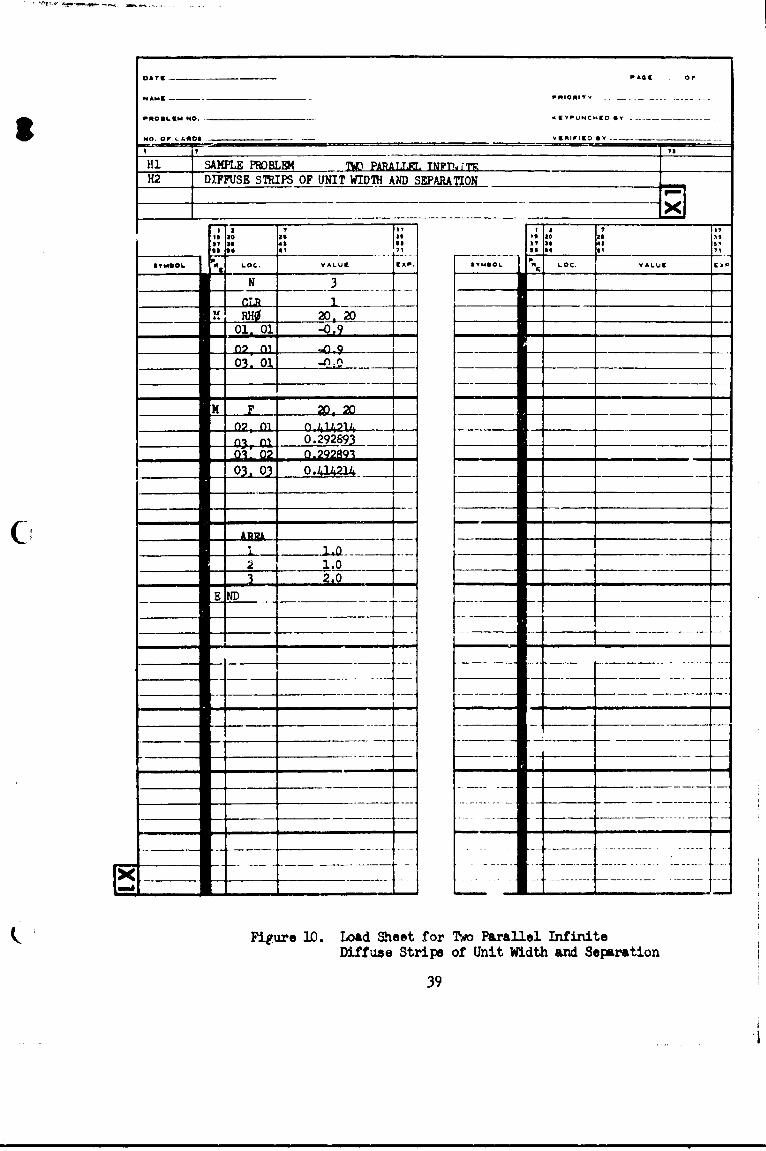
The following is a very simple problem mhich illustrates theinput loading. Consider two infinite diffuse stripe of unit width andseparation, as shown below:

(2)curface (1) and (2)

(3) 1 aurface (3) is space

(1) Pl P2 0.9; P3 0

Input information:

(a) P12 = kI m P21 : P 23 0. 9

P31 = P32 = P33 = 0

(b) F1 2 - F F33 = 0.414214

F1 = F23 0.585786

(c) R2 1 3 : R1 2 =R3 1 3 R22= P 1 0.9

' 1 23 = 321 - 323 = R11 2 =0-9

(d) A1 = A2 = 1.0, A3 = 2.0

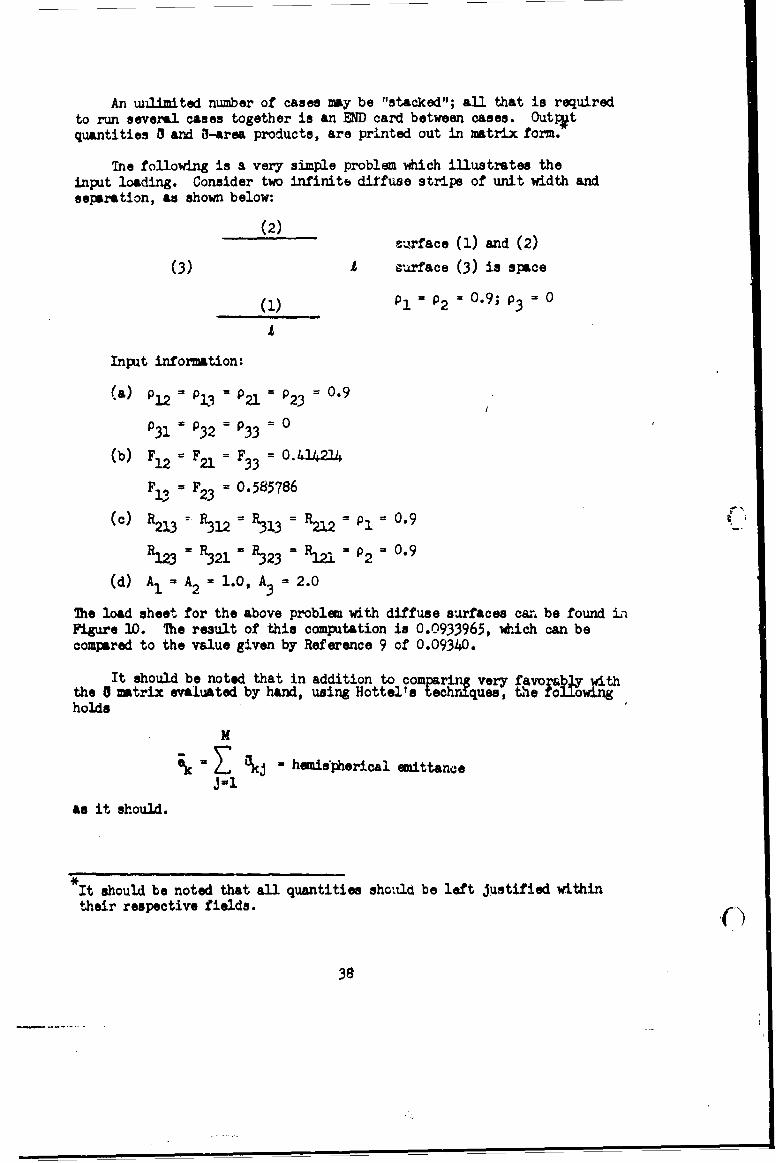
The load sheet for the above problem with diffuse surfaces car be found inFigure 10. The result of this computation is 0.0933965, which can becompared to the value given by Reference 9 of 0.09340.

It should be noted that in addition to comparing very favor&by withthe 0 matrix evaluated by hand, using Hottel's techniques, the followingholds

M

= Z kj - humis'pherical emittance

J-1

as it should.

It should be noted that all quantities should be left Justified within

their respective fields. ()

38

DATE WAGE or

NAM PRIORITY

PROBLEM NO. A EYPUNCHI[D y . .

No. OFw "AINDS

* --- rIFllrO myS -T-V--I.... "" " '_ ___-_

Hi SAMPLE PROBL4 TWO PARATIML TNWh TTF.H2 DIFFUSE STRIPS OF UNIT WIDTH AND SEPARATION

* 17 1 , ,717

• ,IS I4 II 71 5 00

SYMBOL N LOC. VALt

E L ' LOC. VALUE

N 3

01 01 -0.9 ___________

MF 20, 20

n-- 0.292693 1-.

03_ , 0.41 _4_

C _ - I- _. I_ _._ -.......

._ _ _ 2 _ 1.0 ....._----- __.22 -____ _ _ _

3 2.0-- - -

_E ND

- - -- - -J

Figure 10. Load Shet for Two Parallel InfiniteDiffuse Strips of Unit Width and Separation

39

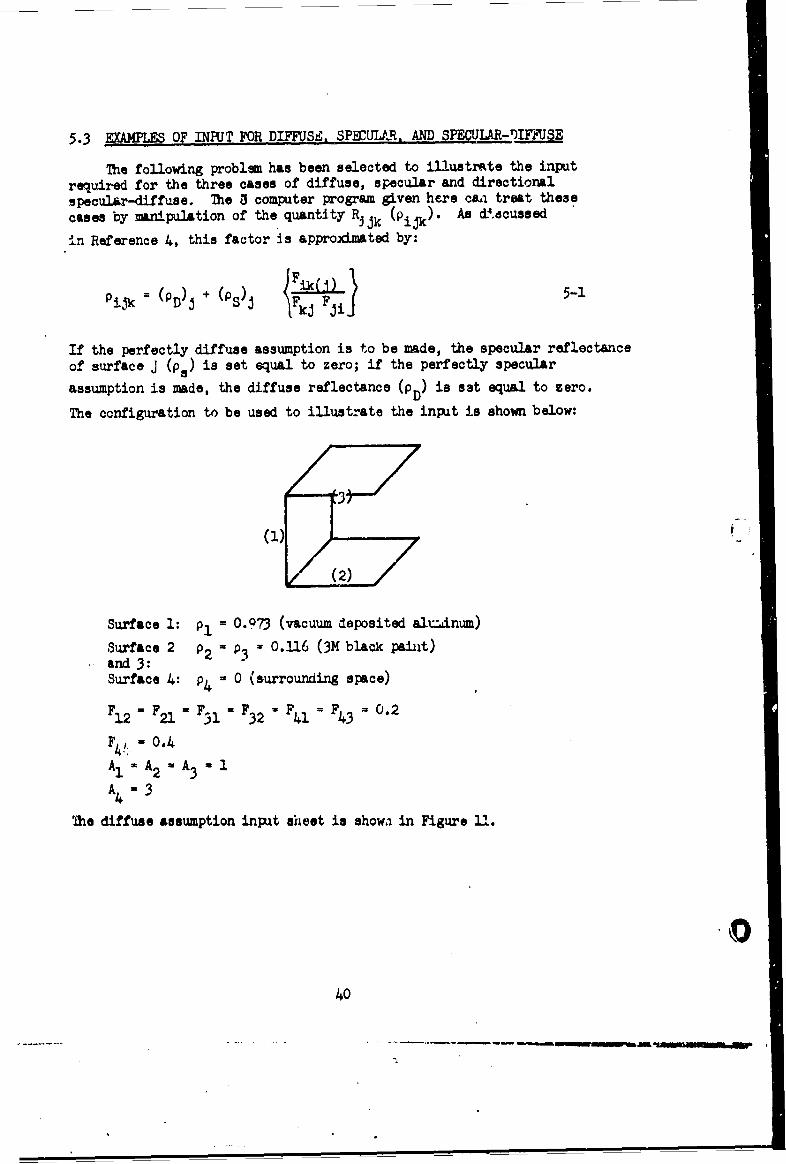
5.3 EXAMPLM OF INPUT FOR DIFFUSE. SP EUL.R. AND SPECULAR-IFFSE

The following problem has been selected to illustrate the inputrequired for the three cases of diffuse, specular and directionalspecular-diffuse. The 3 computer program given here caa treat thesecases by manipulation of the quantity Rj k (Pijk) . As d'ecussed

in Reference 4, this factor is approximated by:

Pijk (D) j + (s)j FkJFJ 5-1

If the perfectly diffuse assumption is to be made, the specular reflectanceof surface J (pa) is set equal to zero; if the perfectly specular

assumption is made, the diffuse reflectance (p D) is set equal to zero.

The configuration to be used to illustrate the input is shown below:

(1

Surface 1: p1 = 0.073 (vacuum deposited alianum)

Surface 2 p2 = p3 = 0.116 (3M black paint)

and 3:Surface 4: P4 = 0 (surrounding space)

23 - F- 1 FF1 -FF =0.2F12 = r.=z3 "=F32 41Fz F43 = .

F4 ! 0.4

A1 1 A2 = A3 - 1

A -3

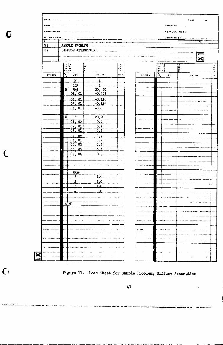
The diffuse assumption input sheet is show in Figure 1.

40

C ~NO o' CAD@ IRFEDB

SAMPLE PROBLPFM__________ ______

H2 DIFFUSE ASSUMPTION _____________

r772 a T 27I o Is* II

20237 ]so .1 137 31 .1

sYMBOL R OC. 7L( {t VAL.~I(7

_ _N -- - ---- -_ _ _

Mg __ _ 20 t20 _ __ _

________ 01, 01. -0.973 ____ _______

_ 02. 01 _ .0_ _ __ _ _ _ _

03 . 0 1. __ -0 .116

_ _ M F 20,20

____ 01, 02 0.2__2 0 0.2_

____.3_ 0 0.2 ____

________ 04, 01 0.2 _ ______

_______ 04, 02 - 0.2 ___

_______ - AREA ___-

2 1.0

- - ----- ----- ---

Figure 11. Load SetfrSmlPob m;Diffuae Aasumptian

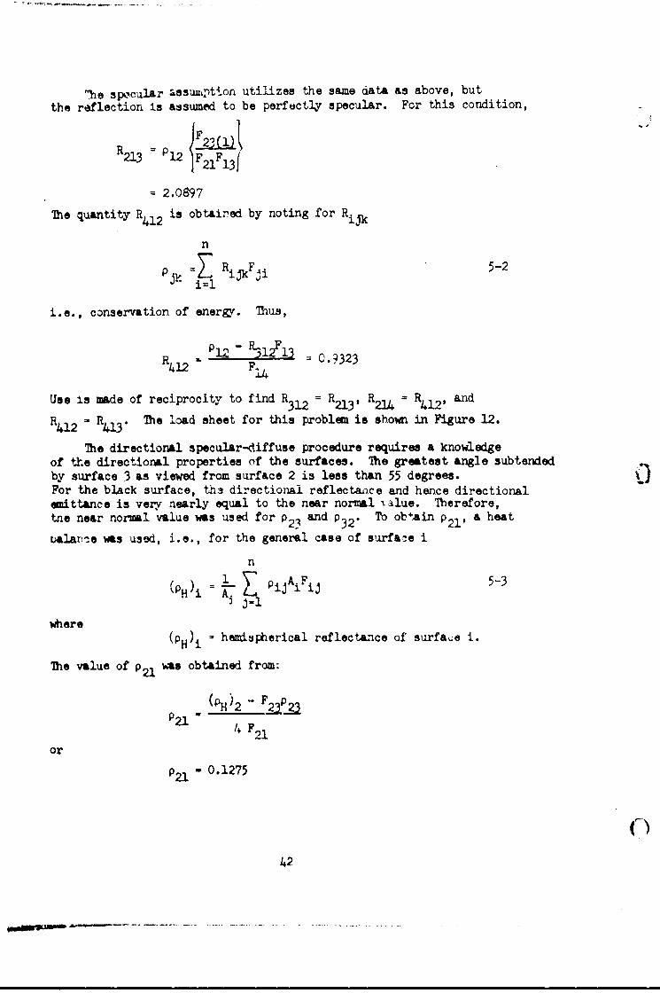
"he spNcular assumptton utilizes the same 'ata as above, but

the reflection is assumed to be perfectly specular. For this condition,

Ra F 2 3 (1)213 12F 2 1 F 1A

= 2.0897

The quantity R41 2 is obtained by noting for Rijk

n

PJk = F RiJkFj 5-2

i.e., conservation of ener&y. Thus,

R41 - 12 - F R1 2F' 3 =- 9323R412 F114

Use is made of reciprocity to find R312 = R213 , R214 = R412, and

R412 = R413 . The load sheet for this problem is shown in Figure 12.

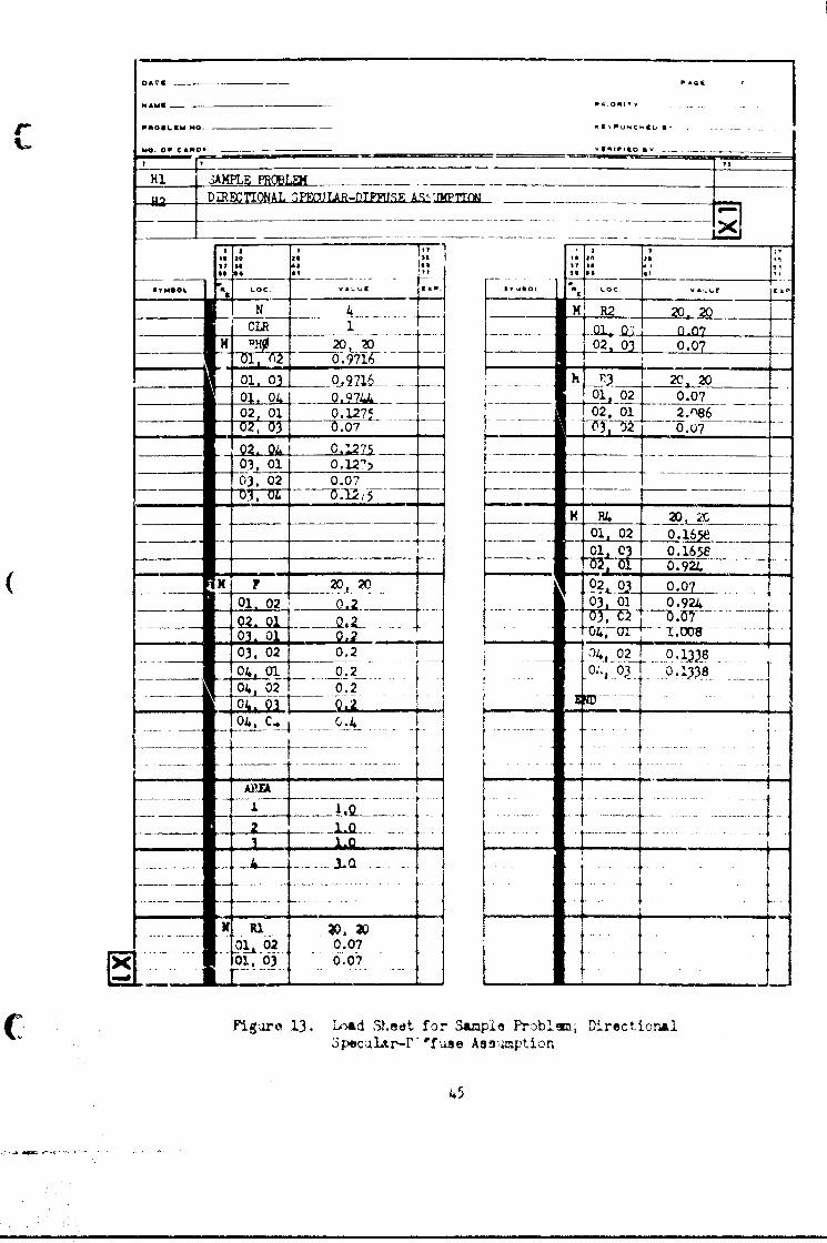
The directional specular-diffuse procedure requires a knowledgeof the directional properties of the surfaces. The greatest angle subtendedby surface 3 as viewed from surface 2 is less than 55 degrees.For the black surface, t213 directioral reflectance and hence directionalemittance is very nearly equal to the near normal Alue. Therefore,tne near normal value was used for p23 and p3 2 . To obtain p2' a heat

ualax)e was used, i.e., for the general case of surface i

n

1.. Z pijAiFij 5-3

where(PH)i . hemispherical reflectance of surfac.e i.

The value of p21 *as obtained from:

P21 - / F,,1

or

P21 " 0.1275

42

mO..NlIO..O T - .... - . .

"o. of, CA .o l JCoIO . .

Hi SAK _______H2 SFPa!LA.R ASStUPTICN

IYI O oz.vl val L C C 4LUE5M R3 20 333-~.. .....' - _ .. . . U .30 ,3Y OL £1 3... V.~( . .V. O.... oALuf (--

-L -- 01l 02 _ 0. 1A_ M 21 _20 02 01 2.0897

01 02 0-3 03.02 06...-- -04 . 4-_....._---- - 41- -

___ 02 01 -0 6

04-01 20

- ~ ~ ~ ~ ~ ~ ~ ~ 1 034 1.1 - - ______

- - r -.......- OI61...2.2 L.....-02 -01

--- - - •- -- Q 2012 -QA-3 -- - U

.02 0.2 0 01 •-2, 01 0.2 _0_ ______

03e0 .2 04 ............04, C , 2 "

- 4. 03 - .2

_ . 46____-________________ __

.... ...

Figure 12. Load heet for Sample Problem; Sp:eular Assumption

43

Reciprocity wat utilized to obtain P21 = PI2 p3 1 p1 3 , etc. Using

the procedure described for P21' the values of the other geometricalreflectances were:

p12 = P13 = 0.9716

P14 = 0.9744

P23 = p32 0.07

The load sheet for this problem is show in Figure 13.Thb computer results for the above configuration will be found inSection 6.

4)

44

4rP 40LIM NO. S -~~Ct .

NO. OF CAP *- - .... . "(, * -*I

DRECTIONAL SF I1AR-DIFFUF A_ MITON

a v0 IS0 L0 ". 13 V -

, 5 _* .C 3 . 03.O , ¥1L [ i -i 3i*I 1 L 1 .LS -- i

r . .l

c__- ; - - ---1l --___ ______N 4 ---- _--M -2H _ o0.o

__ __CLR 1 Z _ _ _ _ _

o . , - 97r --0 ,.97...-1, 03 0_ _ 1o__ 3 .7 _ hF,_20 o20...

0_,41 0 9- 01 02 0.07

03, 01 0.12'_ . ..5_-0___- -3. 02 0.07 -. 07 --

-U ---T] i5 ....

__ __X R4 20,4 _

" __ -... 01 2 0 0.165801-, _03 o. 16 5e--0. 0 0.924

-..... _0 o 0240. 03 1 0.924 ..

_Q2 01 ---- - ,-- -1-&: - ],,

03, 02 0.2- 141 02 0.1)____ 04, 01 _ 0.2 - _ 3 . 8

- 2 0.2

04, . C f. .T--

.. .....- ... .... ....L 4 7-' .. .

02 0.07

Fig rt 13. LIad Sheet for Sample Problem, Directiorl3peciLr-r" "fase AsS.vmption

45

6. EXP'ERIMENTAL COMPARISON OF SPECULAR, DIFFUSEAND DIRECTIONAL SPECULAR-DIFFUSE ANALYSES

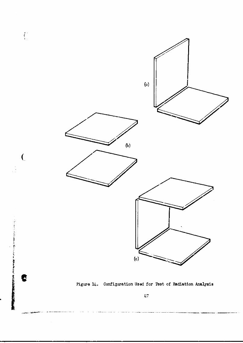
The purpose of this task was to obtain an experimental evaluation ofthe different analytical methods. Such a comparison must utilize anexperimental system that is simple coaceptually and physically. Other-wise the effects of geometrj, conduction, convections, extraneous heatlosses, etc., will not be controlled. The experimental configurationschosen are -houm 5n Figure 14. A test consisted of placing the experimentwithin a c' -d wall vacuua chamber (to eliminate convection), insulatingthe non-raa& etive surfaces, supplying a known quantity of power to oneof the surfaces and measuring the equilibrium temperatures of the othersurface(s). The experimental results were then compared to the predictedvalues using the directional specular-diffuse analysis (4), the specularproperty assumption and the diffuse property as!umption.

The following discliision will be divided into three parts: (1) the,xperimental test method, (2) the analytical results, and (3) a discussionof the comparison of experiment and mnalysis.

6.1 EXPERIMTAL MEIHOD AND PROCEDURE

The configuration L lected for test are shown in Figure 14 Thetest surfaces %ere 3ix such squares of 3lOO aluminum 0.0625 inc. thick.in each case the lower surface was selected as the heat source ana theremaining surface(s) allowed to reach an equilibrium condition with theenvironment. The heated surface had a heater of approximately 200 ohmscemented to its 1underside (the non-radiative side). This he.er consistedof 40 gage constantan wire sandwiched between two sheets of 1 mil Mylar.Voltage leads were attached at the heater boundary and the four terminalresistance method used (sje Section 3.1) to calculate power dissipation.The electrical neasuring circuit was the same as shown in Figure 6 ofSection 3 with a Leeds and Northrup 8686 substituted for the Type K 3.

Originally, tbe back of each surface was insulated with 20 layers ofsuper insulation. However, the edge heat leak was Lound to be too largerelativea to the heat absorbed hy the unheated surfaces. A guard heatsystem was found to be necessary. This was obtained by placing a heatedplate on the outside of the insulation and adjusting the dissipation untilte temperature difference across the insulation was zero, i.e., no heatflow through the iniulation. The edges of the insulation, guard heater,and test surface were cc'.-%.red with 1/4 mil thick aluminized Mylar,aluminum side ouu. These steps reduced the edge and back heat "leak,"i.e., uncontrolled loss, to approximately I Btu/hr for a test surfacetemperature of 70 0 F. This was satisfactory for all test surfaces excepLthe surface coated with vacuum deposited aluminum. The radiative heat lossor gain from such a surface was the same order of magnitude as the edgeloss. Hence, thia test surface had to be used as a passive surface, i.e.,a reflector, and no heat balance could be performed for it.

46

(6)

(c)

Figure 14. Configuration Used for Test of Radiation Analysis

47

-- --- --

Fieiire 15. Test Conf'iguraticmn in Test Pixture

48

Figur'e 16. Test. Confi.gu.ration Reaely f or Testing

49

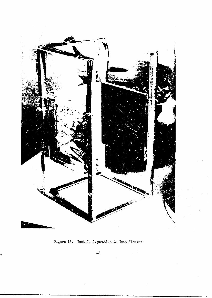
Each test surface was supported within a framework by dacroncords attached to phenolic stand-off attachments. In this mannerthe test surfaces were isolated from the framework but properly positioned

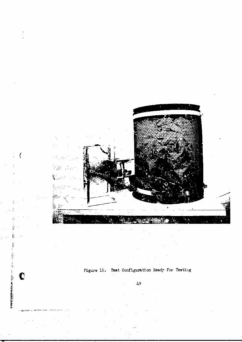
and restrained (see Figure 15). This framework was mounted within a LN2cooled baffled tnd the assembly placed within a vacuum system. A

pressure of 10- torr or lower wa2 obtained during the testing. The systemis illustrated in Figu-e 16.

Thermocouples -were placed on at least two points of each test gurface;one at the csnter of the surface and one within one-half inch of the edge.No significant gradient across the test surface was observed in any of the testa;

i.e., the surfaces were essentiAlly isotiermal. The thermocouple material wascopper-constantan. All thermiccouplos were taken from the same roll. Thevoltages generated by the thermocouples were measured with a Leeds andNorthrup Type 8686 potentiometer using a conventional ice J-Xictiorn compensationsystem.

The test procedure consisted of the follcwing steps:

(1) setting the predicted power dissipation for the source surface

(2) setting estimatsd guard heat dissipation(s) for the receivingsurface(s)

(3) obser-ving the temperature of the receiver surface(s) andadjusting the guard power dissipation(s)

(4) when the receiver surface(s) and guard heater(s) indicateda negligible temperature difference for thirty minutes,at least two sets of data were recorded within the next6hirty minutes.

The latter step insured that the surfaces were in equilibrium for

appro.mately one hour. The accuracy of the measurements ars estimatedto be:

Temperature difference + O.lFTemperature - FTotal power disipated by 1.5%the heat source

A complete du"ma A of the experimental data is given in Appendix III.

6.2 ALY AL PREDICTICM

The radiative heat flow from the source surface and the temperatureof the receiver surface were predicted by the analytical methods

based upon the three different property assumptions: diffuse (J.,2,j),specular (7), and the directional specular-diffuse (4). The predictionserved to test the utility and practicality of the computer programdeveloped for this study (Sectlon 5) as well as provide a basis ofcomparison between theory and experiment.

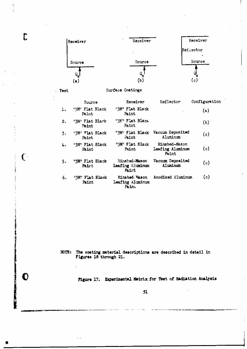
Me test configurations have been described in Section 6.1 andillustrated in Figure 14. These three configurations were combined withdifferent surface coatings to give six different test system. Thesesystems are schematically represented in Figure 17. The directional

- 50 -

Receiver Receiver Receiver

ReLfector

Source Source Source

QS

(a) (b) (c)

Test Surface Coatings

Source Receiver Reflector Configuration

1. "3M" Flat Black "3M" Flat Black (a)Paint Paint

2. "3M" Flat Black "31P" Flat Black (b)Paint Paint

3. "3M" Flat Black "3M" Flat Black Vacuum Deposited (c)Paint Paint Aluminum

4. "3M" Flat Black "3M" Flat Black Rinshed-14asonPaint Paint Leafing Aluminum (c)

Paint

5. "3M" Flat Black PM shed-Mason Vacuum Deposited (c)Paint Leafing Aluminum Aluminum

Paint

6. "3M" FIAt Black Rinshed- Mason Anodized Aluminum (c)Paint Leafing Aluminum

Paint

NOTE: The coating material descriptions are described in detail inFigures 18 through 21.

U Figure 17. Experimental Matrix for Test of Radiation Analysis

51

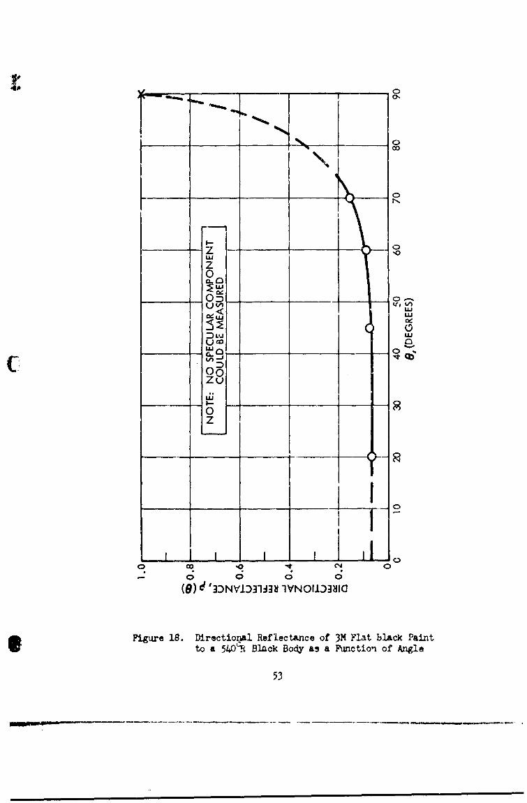
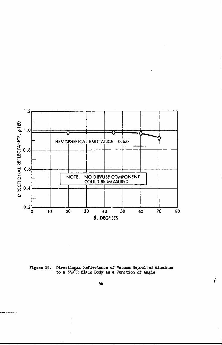
reflectances of these coatings for a black body s urce at 540 R areshown in Figures 18 through 2L. Included in these figures is the specularreflectance for the same radiation source. The specular reflectances weremeasured with a goniometric reflectometsr shown in Figure 22. Thedirectional reilectances were measured with a heated cavity reflectometersimilar to that described in Reference 11.

The method of determining tha various quantities and establiahingthe input for the computer program has been described in Section 5.3.The results of the computer calculations are sho,'n in '.ble 7.

6.3 COMPARIS014 W7 EXPERIMTAL AND ANALYTICAl. .SULT

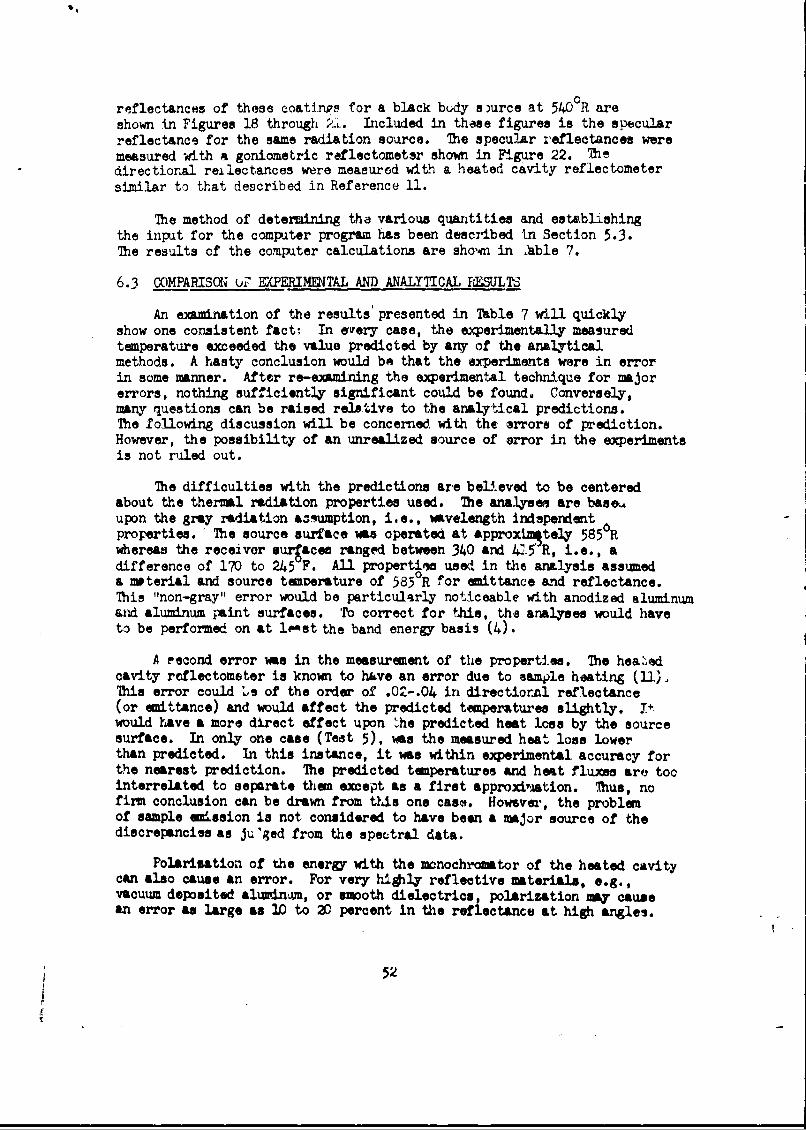
An examination of the results' presented in Table 7 will quicklyshow one consistent facti In euery case, the experimentally measuredtemperature exceeded the value predicted by any of the analyticalmethods. A hasty conclusion would be that the experiments were in errorin some manner. After re-examning the experimental technique for majorerrors, nothing sufficiently significant could be found. Conversely,many questions can be raised relstive to the analytical predictions.The following discussion will be concerned. with the errors of prediction.However, the possibility of an unrealized source of error in the experimentsis not ruled out.

The difficulties with the predictions are beleved to be centeredabout the thermal radiation properties used. The analyses are base,upon the gray radiation a-umption, i.e., wavelength independentproperties.' The source surface is operated at approxtmtely 585 Rwhereas the receiver surgaces ranged between 340 and 45 R, i.e., adifference of 170 to 245 F. All propertimA used in the analysis assumeda nmterial and source temoerature of 5850 R for emittance and reflectance.This "non-gray" error would be particularly noticeable with anodized aluminumand aluminum paint surfaces. To correct for this, the analyses would haveto be performed on at lest the band energy basis (4).

A second error ws in the measurement of the properties. The hea ,edcavity reflectometer is known to huve an error due to sample heating (11).This error could 's of the order of .02-.04 in directiorzl reflectance(or emittance) and would affect the predicted temperatures slightly. I +

would have a more direct effect upon 'he predicted heat loss by the sourcesurface. In only one case (Test 5), was the measured heat loss lowerthan predicted. In this instance, it was within experimental accuracy forthe nearest prediction. The predicted temperatures and heat fluxes are toointerrelated to separate them except as a first approxid'ation. Thus, nofirm conclusion can be drawn from this one cas. However, the problemof sample emission is not considered to have been a major source of thediscrepancies as ju'ged from the spectral data.

Polarisation of the energy with the monochrormtor of the heated cavitycan also cause an error. For very hithly reflective materials, e.0g.,vacuum deposited alurin-m, or smooth dielectrics, polarization May causean error as large as 10 to 20 percent in the reflectance at high angles.

52

0'

Kz 1:10

ZO

0zo - ---

CL

05 0

U j CC

5:253

S LU ." I I0 C 0

(0 U1Nj .:1=]11 N I3 l

Figre 8.Dirctona Rfletane f 3 Fat lak Pin_--- to a 0 lc oya ucino nl

z5

L , :

1.2

S1 .0u _Z HEMISPHERICAL EMITTANCE = 0.027

0.8U

LU-J

-j 0.6zo NOTE: NO DIFFUSE COMPONENT

COULD BE MEASURED,, 0.4

0.2 -

0 10 20 30 40 50 60 70 809, DEGREES

Figure 19. Directiely Reflectance of Vacuum Deposited Aluminumto a 540 R Elack Body as a ihuction of Angle

54

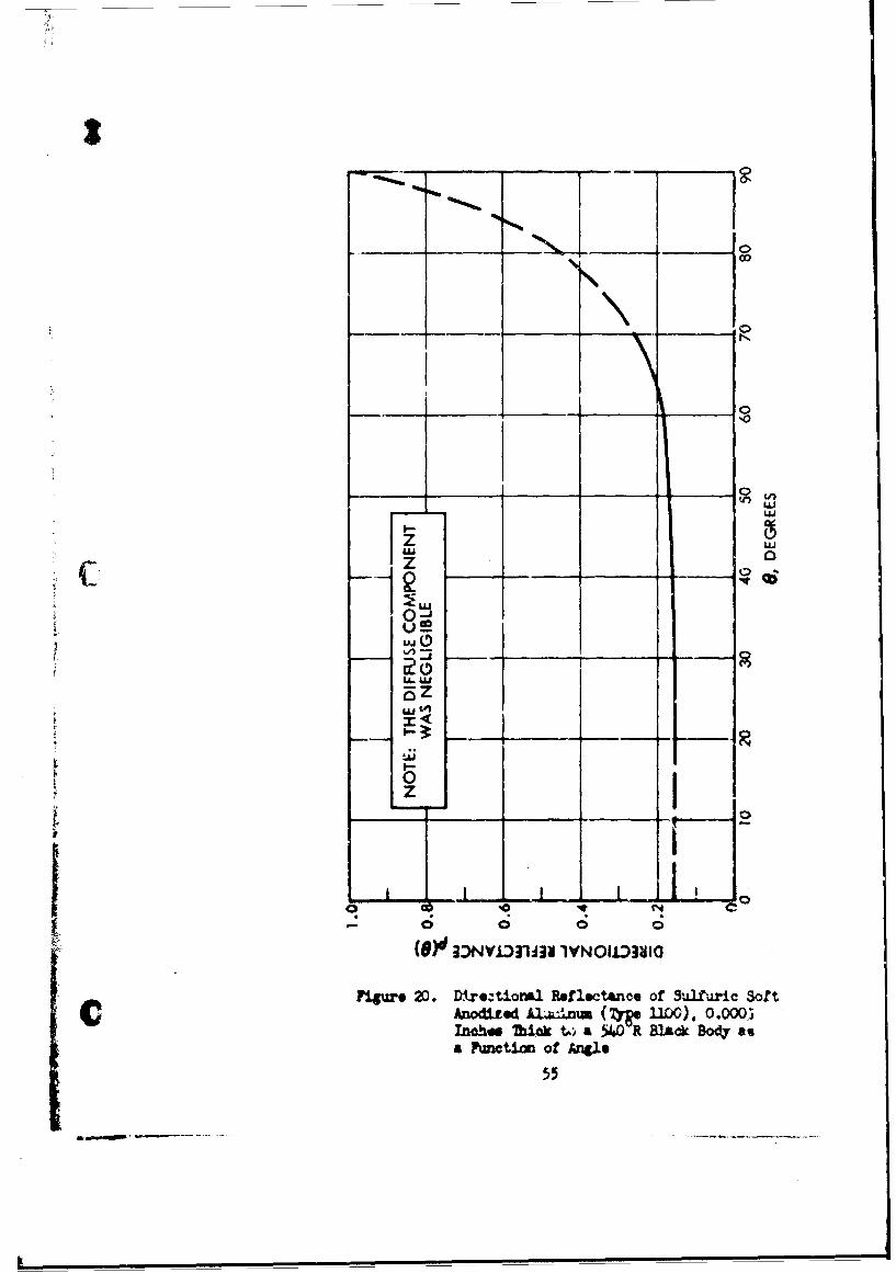
.44

SLI--j

U.",

14 ~~~L- _______

I - hI

o 0

( 9d NYIT3 1V N01Ii)3VIO

Figure 20. Dixv-tioml Reflectance of Sulfuric Sof tAnodized Alj .ni (71s 1IDG), O.oOOCThhe hik to a R BlakBody asa ?uncticm of Angle

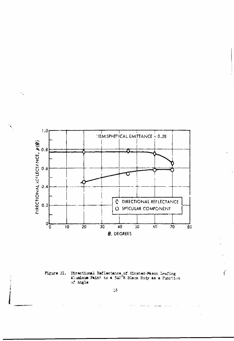
1.0 -

'IEMISPHEP1CAL EMITTANCE =0.28

z

-

0.4-

z0___

CDIRECTIONAL REFLECTANCEat_ 0 SPECULAR COMPONENT

0 10 20 30 40 30 60 70 80

9, DEGREES

Yigure 21. DirectiurAL Reflactazxe of P.ished-Mason LeafingA,-mini2 Paint to a 5400H B2Ac-k Boly, as a IPunctio1'! Angl1e

56

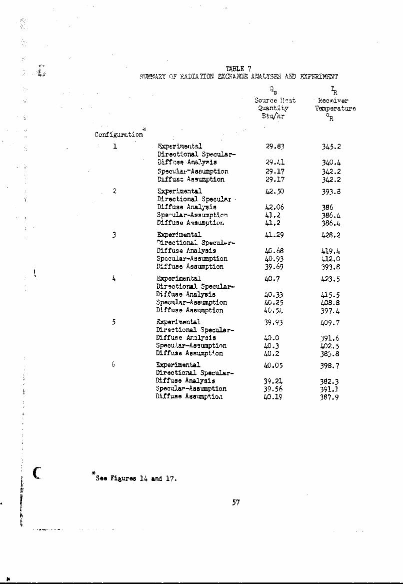
TABLE 7CFTA~ QEADIATON ATIALYSF AIND FRF'TflOT

0 TR"our-e t Yec,'iverQantitir Temperature

0 R

Configamtion

1 Kneorimental 29.83 345.2Diret.-tional Specular-Di f i An&Ay-Is 29.41 340.4Speculai.,Asrumption 29.17 342.2Diffuse Asgumption 29.17 342.2

2 Experimental 42.50 393.8Directional Specula zrDiffuse Analysis 42.06 386Spe-ular-Assumpticn 41.2 386.4Diffuse A-sumptior, 41.2 386.4

3 Eerimental 41.29 428.2rjirectiona. Specular-Diffuse Analysis 40.68 419.4Spccular-Assumption 40.93 "12.0Diffuse Assumption 39.69 393.8

4 Experimental 40.7 423.5Directional Specular-Diffuse Analysis 40.33 415.5Specular-Assumption 40.25 408.8Diffuse Assumption 40.54 397.4

5 Experimental 39.93 409.7Directional Specular-Diffuse Analysis 40.0 391.6Specular-Asumption 40.3 402.5Diffuse Assumption 40.2 383.8

6 Experimental 40.05 398.7Directional Specular-Diffuse Analysis 39.21 382.3Specular-PAsumption 39.56 391.)Diffuse Assumptioa 40.19 387.9

i*

IC See Figures 14 and 17.

57

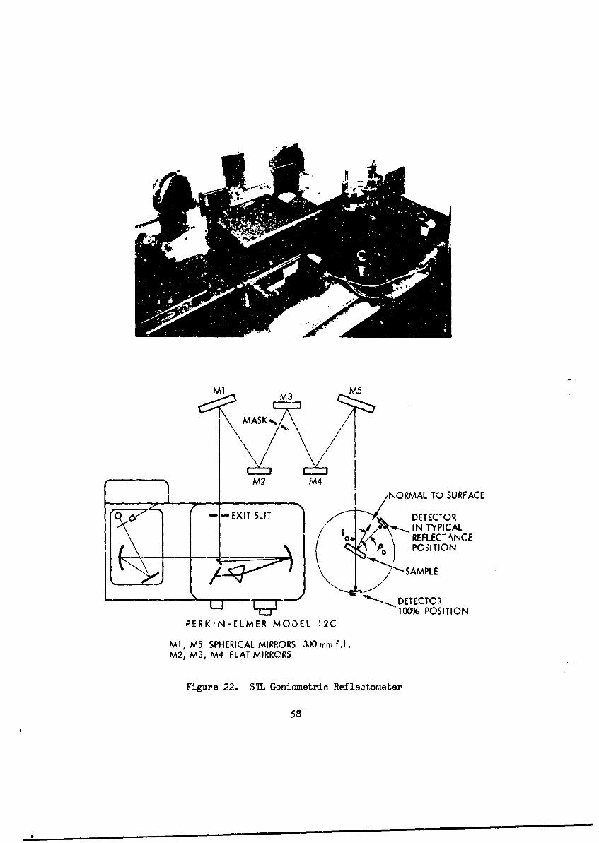
Ml M3M5

MASK

i2f M/NORMAL TO SURFACE

-EXT LI DETECTOR- 0 IN TYPICAL

00 REFLECANCEPo POSITION

SAMPLE

SDETECTOI100% POSITION

PERKiN-ELMER MODEL 12C

MI, M5 SPHERICAL MIRRORS 300 mm f.l.M2, M3, M4 FLAT MIRRORS

Figure 22. STh Goniometric ReI'1ectoneter

58

This source of error has also been recently recognized and the informationrequired to assess this error is not yet available for the monochromatorused, In the case of the tests described, only t'e 3M flat black paint willbe free of this error.

A fourth source of error was ths approximations used to obtain thegeometrical reflectances; i.e., the interaction between spatial variationof reflectance and the shape factor integral. The methods used toapproximate these properties have been described in Section 5.3. Until aspatial distribution of the reflectance propeety of a number of surfaceshave been obtained and incorporated in the integration of a shape factcr,the magritude of this error will not be known. Simple analysis of anextreme case has shown this to be as large as 30 percent (4).

Considering all of these factors together, plus the probableexperimental error, leaas to the conclusion that the predicted temperaturesshould Ue re-examlined. This would require the analyses to be performedon a band energy basis and with a more detailed evaluation of tha properties.

The analytical results given in Table 7 also offer an opportunity tocompare the different methods of analysis. The program described inSection 5 is based upon the method given in Reference 4. The technique isan admitted approximation to the integral equations describing the radiationexchange within an enclosure. The other two methods are also approximationsin that an assumption is made relative to the radiation properties, i.e.,nondirectional perfectly specular or perfectly diffuse. The approach

(programed to this stidy resulted in a set of equations which were verysimilar to those .jtained in the diffuse approxdmation and could be solveawith a slight _ ucrease in time. In contrast, an enclosure with perfectlyspecular surfaces can require extensive preliminary calculation to obtainthe "specular interreflections."

The test configurations of Figure 17 are examples of very simpleenclosurGs which are easily solved by any one of the three methods. Theydo not represent a complex enclosure and cannot adequately demonstratethe differences between the specular, diffuse and directional specular-diffuse methods. A trend can be inferred, however. For example, TestConfigurations 1 and 2 should yield ident cal results for the specular anddiffuse assumptions. The directional specular-diffuse analysis yieldsdifferent results because the emission from source occurs at iargt anglesfrom the normal. The predicted temperature of the recoiver is higher forTest 1 and lc:wer for Test 2 because of the angular effects ef absorption.

For Test 3, the specular analysis is suitable but does not acco,.Mt for thedirectional properties. The diffuse analysis does not account for specularreflection and radiation is 'diffusely" reflected back to the source. Thedirectional specular-diffuse result is between these two. SimiLararguments htld for Test Configurations 4, 5, and 6. These geometries aremore complicated by the use of the alumirul paint and anodized aluminumwhich have directional and/or specular components of reflection. In morecomplicated enclosures, such a simple explanation of possible differencesis not practical. The only comment that car. be made is that the directionalspecular-diffuse analysis is a more realistic approximation to physicalfact.

*1 59

7. CORREIA7I OF COIUPENT JOINT ECEPIMTAX1 RESULTS

At the request of the Technical Monitor, C. J. Feldmanis, an effort;ws made to correlate the experimentally measured valses of jointconduction. This work was a substitute for the completion of thepreliminary design task originally scheduled for the last portion of theprogram. This correlation effort has resulted in a simplified approachbased on the conduction flow pattern to a circular cavity(region of thebolts) in the mating par'ts. For the thin plates in the component mountingjoints, the conduction at the bolts was very high and the apparentcontact area small. This led to the conclusion that macroscopic effectswere of the greatest significance.

A review of the technical literature revealed little informationthat would be useful in predicting interface conductance for the boltedjoints of this study. A subsequent study of the pressure distributionindicated that the apparent contact area occupies only to a small regionnear the bolts. This suggested that the predominant thermal resistancelies in the mating plates themselves. This correlation effort hasresulted in a simplified expression for the interface conduchance basedon the heat flow pattern in a large circular region to a circular sinkat the center. These comments apply specifically to the mountingplate configuration investigated in this study.

7.1 REVIW OF LITERATURE

A review of technical literature reveals that the study of vacuum thermalcontact resistance is of recent vintage. Past emphasis has been uponjoints in a conducting fluid; e.g., air. This is not surprising sincethe need for information on the behavior of heat flow through connectingelements in a vacuum was not great until the advent of satellites. Anexcellent review of technical literature ic contained in Reference 12 anda bibliography on contact conductance is contair.d in Reference 13;Appendix V list references that are not reported in Reference 13.

As background to the correlation to be presented, two well knownmethods that have been proposed will be cited. The applicability (orlack of it) to the type of joints considered in the present study will beindicated.

Fenech and Rohsenow (14) developed an expression for the thermalconductance of a mathematical model with contacting surfaces idealizedas cyiindrical contacts eqx.11y spaced in a triangular array. The thermalconductanco was expressed in terms of tho thermal conductivity of theetals and of the fluids of filling the voids, the real area in contact,

the number of contact points per unit area, and the volume average thick-ness of the void gaps. A method of obtaining these physical properties ofa contact is contained in Reference 15. The need foe- the profiles of thecontacting surfaces precluded the examnation of this method.

60

i s

While most investigators were concerned with microscopic areas ofcontacts (those due to surface finish), Clausing and Chao (12) concludedthat macroscopic resistances (that due to large scale waviness or non-flatness) was predominant over the microscopic resistance for a majorityof engineering surfaces. The interface conductan3e was expressed in termsof the mean thermal conductivity of the two contacting materials, theradius of the macroscopic constriction ratio, the contact pressure, themacroscopic constriction ratio, the harmonic mean of the moduli of thetwo-contacting materials, and the total equivalent flatness deviation.This method requires the measurement of flatness deviation and surfacefinish; the latter is readily obtained, but the former is more difficultto measure. This method was not applied since subseqtent studies showedthat the apparent contact area (the region adjacent to the bolts) rel' esentsonly a small percent of the total joint area. However, the concept ofconstrictive heat flow is employed in the present study, except that it isapplied in a much larger, gross scale. The method is discussed below.

The two methods discussed above considered a physical system withouta disruptive element such as a bolt. Intuitively, the influence offasteners should be great. An attempt at correlating joint conductancedata is reported in Reference 16, and the resultant expression is semi-empirical. The method employed in the present study is semi-analyticaland the close correlation with experimental results strongly suggests thatthe governing resistance is centered in the plate itself; at least for thetype of joints considered here. The analytical method is discussed below.

( 7.2 ANALYTICAL DEVLOP=NT

The correlation of joint conductance data was limited to the componentjoint configurations. An anlytical model was postulated based on the workdone by previous workers, experimental data and engineering judgement.The basic concept of the proposed method is that the controlling thermalresistance is tha plate. It is postulated that the points of contactwhich contribute to the conductance are in the small region under andaround the bolts. The problem is then to describe the heat flow in theplate to the bolt area. Two mathematical models were employed for thispurpose.

7.2.1 ANALYTICAL 10DEL I

The first model is shotti in Figure 23(a). It is a disc withuniform heat flux over its surface and conduction to a central area at aconstant temperature. The outside surface (r = R) is assumed to beinsulated. This model is used to describe heat flow in a joint with onlya few bolte in relation to the total area.

6C61-

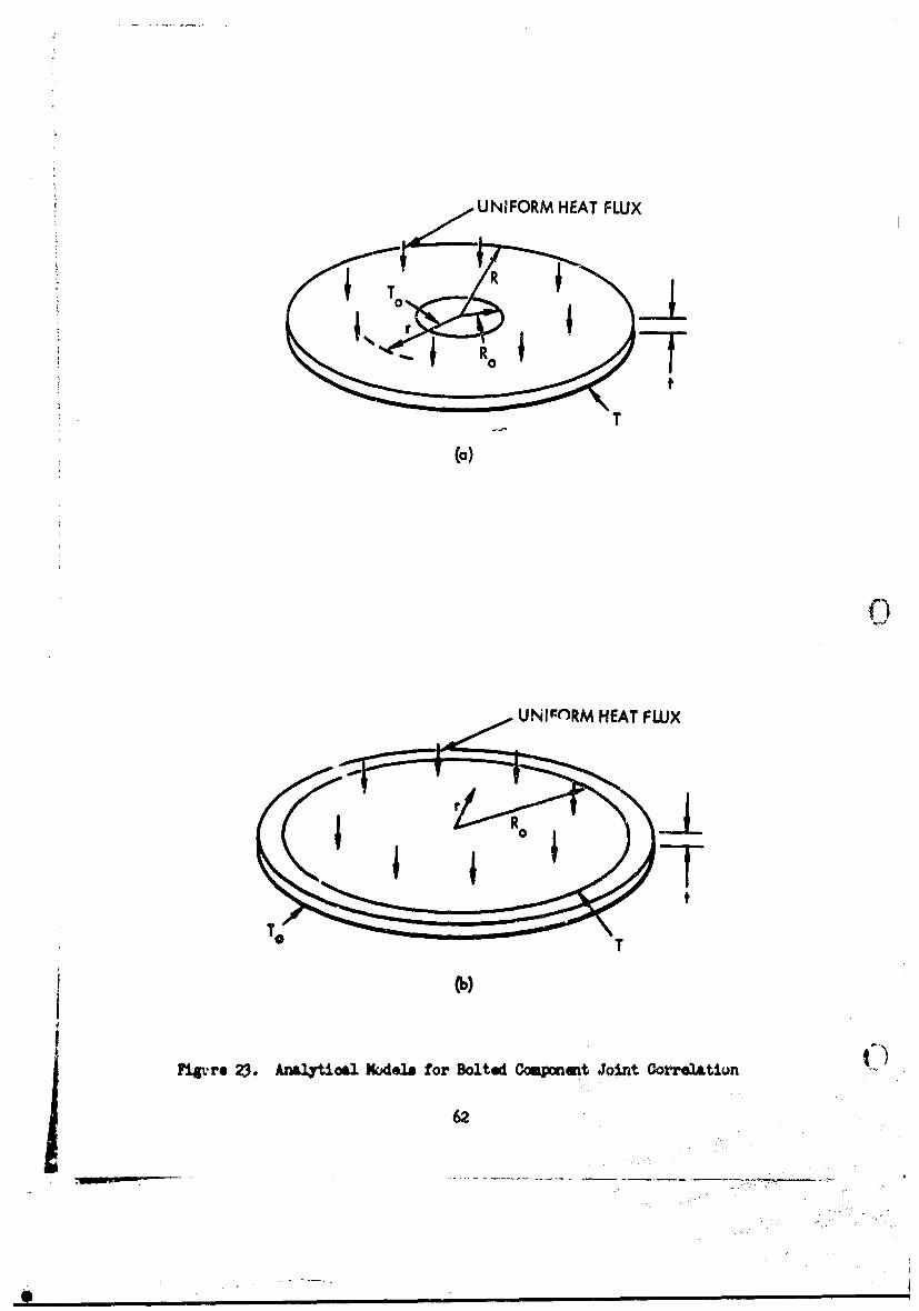
UNIFRM HEAT FWX

TTt

(bT

UNFR HA W

?iii~r. 23 Ana2Lyt~ol Nc~ela fr otdCmnetJitGr]tn

62

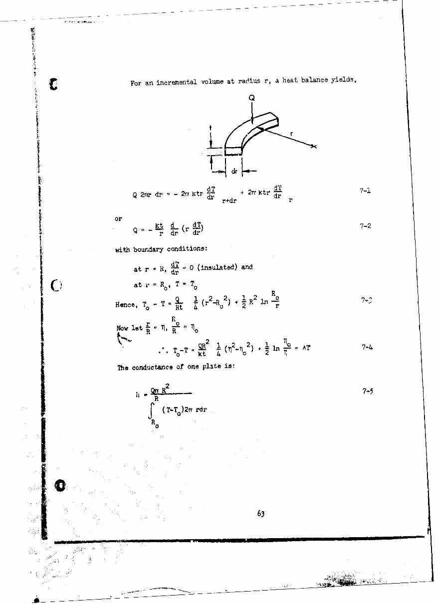
C For an incremental volume at radius r, a heat balance yields,

Q

Ld TIT7

Q 2rdr -2tr~Cty, +2Trctr-A~ 7-1Q r+dr d r

f or

Q=-_ (r ) 7-2

with bourdary conditions:

at r - R, 0 (insulated) andat -- Rdr -10 at '- R, T ToSHance, To T t 4- 0 2 !rTR t= 0 r2o)+7R2 R -

R

Now let Ti, =

o kt 42 + l ? 7-

The conductance of one plate is:

QI 27-5

IR J"(T-To)2.Yrd

CR

63

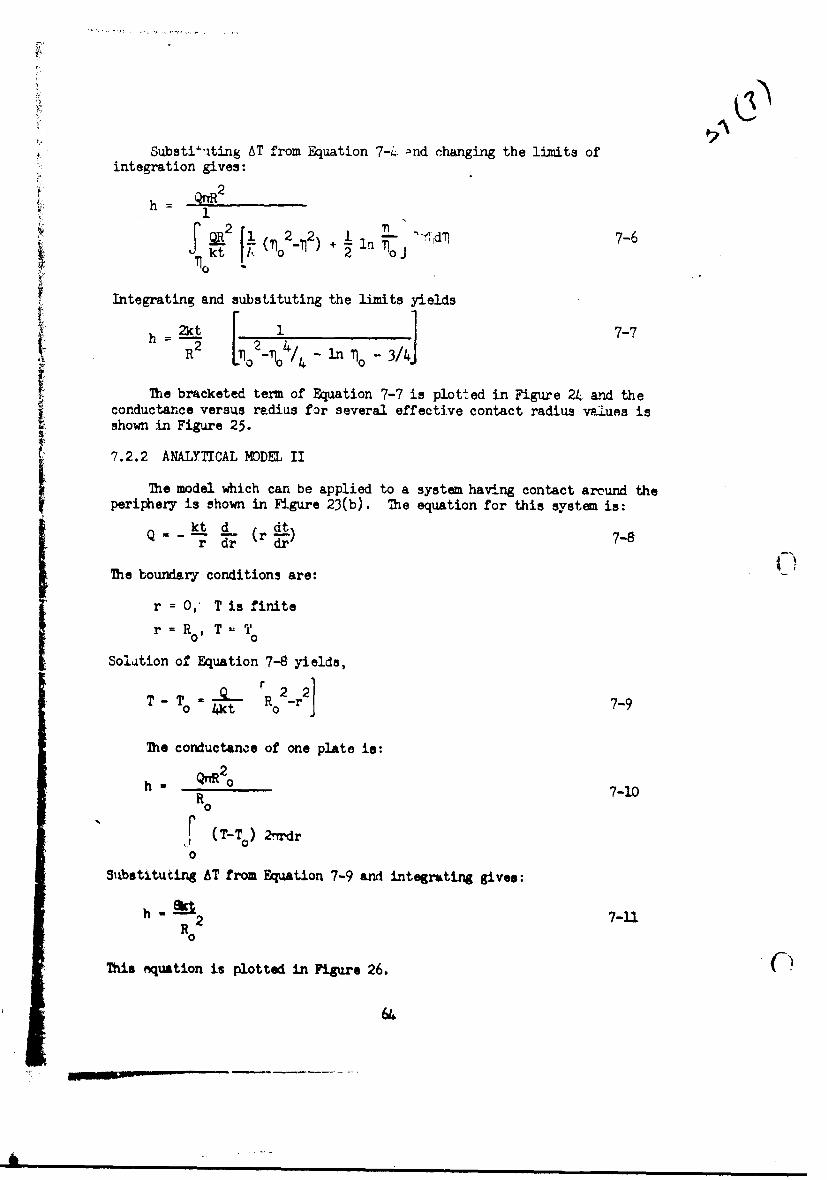
Substi"ting AT from Equation 7-L. 'nd changing the limits ofintegration gives:

h= 1

) +2_12' 7-6f Jt . 2 %J

Integrating and substituting the limits yields

R 2-% 4/ - Tn 10 - 3/4.7

The bracketed term of Equation 7-7 is plotted in Figure 24 and theconductance versus radius for several effective contact radius vaiuss isshown in Figure 25.

7.2.2 ANALYTICAL MODEL II

The model which can be applied to a system having contact around the

periphery is shown in Figure 23(b). The equation for this system is:

Q kt d dtr- dr (r ) 7-8

The boundary conditions are:

r = O,' T is finite

r =RT-T0

Solution of Equation 7-8 yields,

T- To R 2_r 2 7-9

The conductance of one plate is:

h- Qnr2 0 73.0

(T-%0 ) 2rfrdr0

Substitutirg 6T from Equation 7-9 and integrating gives:

7-11R 2

This equation is plotted in Figure 26.

64

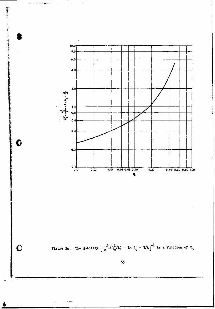
8.0 - _ __ _ _ _

6.0 - __- _ _

4.0 12.0 -__- I

.00.

0.6

0.4

0.01 0.02r 0.04 0.06 0.06 0.10 0).20 0.40 0.60 0.80 1.00

0Figure 24. The Quantity ill20 1CC 4) - in 10 3/4J a a Ftnction of

65

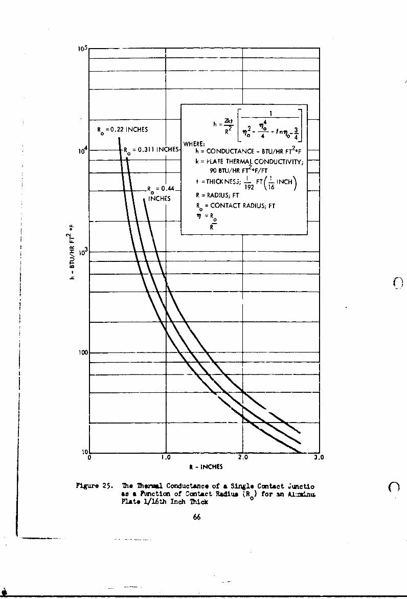
105-

R=0.22 INCHES hR 7 n,

14R = 0.311 INCHES WHERE: F2F10 Ii~~ = CONDUCTANCE- T/RF 0

k = P~LATE THERMAL CONDUCTIVITY;90 BTU/HR FT2-F/FT

I t =THICKNESS; I2~ FT I 2~ NCH0 =.44192 16 )

INCHES R =RADIUS; FTR 0=CONTACT RADIUS; FT

U- R

Cl-

100 _ _ _ _ __ _ _ _ _

0. 2.03.It - IN4CH[S

Figure 25. The Thew.1 Conductance of a Single Contact wunctio (an a ?imction of Contact Raiu R 0 for an Aizzinu%Plate 1/16th inch Thick0

66

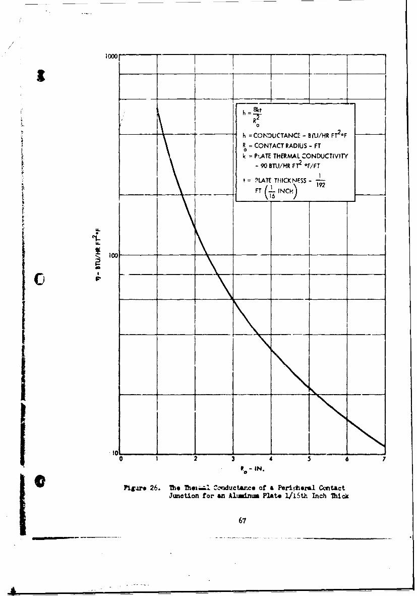
h- 4 1CNUCAC -. 1.UH F-R = CONTACT RADIUS - FT0

k = N-ATE THERMAL ZONDUCTIVITY

-90 BTU/HR FT2 -F/FT

t PLATE THIICK NESS C 19

________ ____FT I. INCH) _____

frr

IL.

~10

10L7I 2 34 5 7

fg*26. The Thri Z, -dvctance of a Peritral~ CwtactJumction for an Alunm PlAto 1/16th Inch~ Thick

67

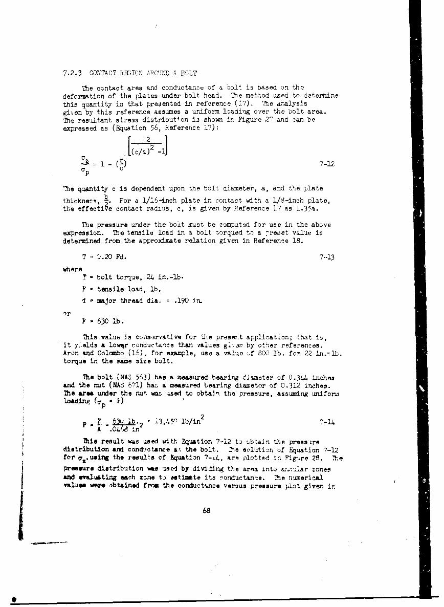
7.2.3 CONTACT RGITON AROULW A BOLT

The ccntact area and conductance of a bolt is based on thedeformation of the plates under bolt head. !he method used to determinethis quantity is that presented in reference (17). The analysisgiven by this reference assumes a uniform loading over the bolt area.The resultant stress distribution i3 shown ir Figure 2- and can beexpressed as (Eq',wtion 56, Reference 17):

JT 2 -

= 1 -()71Cp C

'The quantity c is dependent upon the bolt diameter, a, and the plate

thicknes, b For a 1/16-inch plate in contact with a 1/8-inch plate,the effective contact radius, c, is given by Reference 17 as 1.35a.

The pressure under the bolt must be computed for use in the aboveexpression. The tensile load in a bolt ;orqued to a :reset value isdetermined from the approximate relation given in Referenze 18.

T = :.20 Fd. 7-13

where

T - bolt torque, 24 in.-lb.

F = tensile load, lb.

d - major thread dia. = .190 in.

orF - 630 1b.

TMis value is cc;esr-ative for tje preser~t application; that is,it yields a lowqr ronductance than values givfn by other references.Aron and Colodbo (16), for example, use a value cf 800 lb. fo' 22 in.-lb.torque in the same size bolt.

The bolt (NAS 563) has a measured bearinr djameter of 0.344 inchesand the nut (NAS 671) ha. a measured bearing diametor of 0.312 inches.The area uder the nut w "d to obtaP the pressure, assming uniform

Loading (,p a F)

P 7 1- l3,4 lb/in2 "-14A-W .C in2

Ddie result was sed with 3qation 7-12 to obtain the press iredistribution and conductance ar. the bolt. -he soluti"r. of Equation 7-12for a uing the resule cf Equation 7-14, are plott.d :In Fig.re 29. The

presure distribution we used by dividing the arta into -roiar tones

and waluatir each isne t. astimate its nonductxn:e. The numericalvalus wre obtained from +he conductance verxus pressure plot given in

68

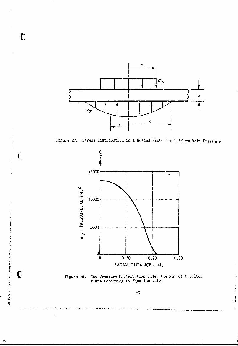
CC

I f I b

Figure 27. S'ress Distribution in a Bclted Plai. for Unifrm Bolt Pressure

15000 -

z 1"

LUV1o0

LU

b

00.10 0.20 0.30

RADIAL DISTANCE - IN.

Figure ,. The Preisure Distribution Under the Nut of r '3oltedPlate Accordiag to Equation 7-12

69I'

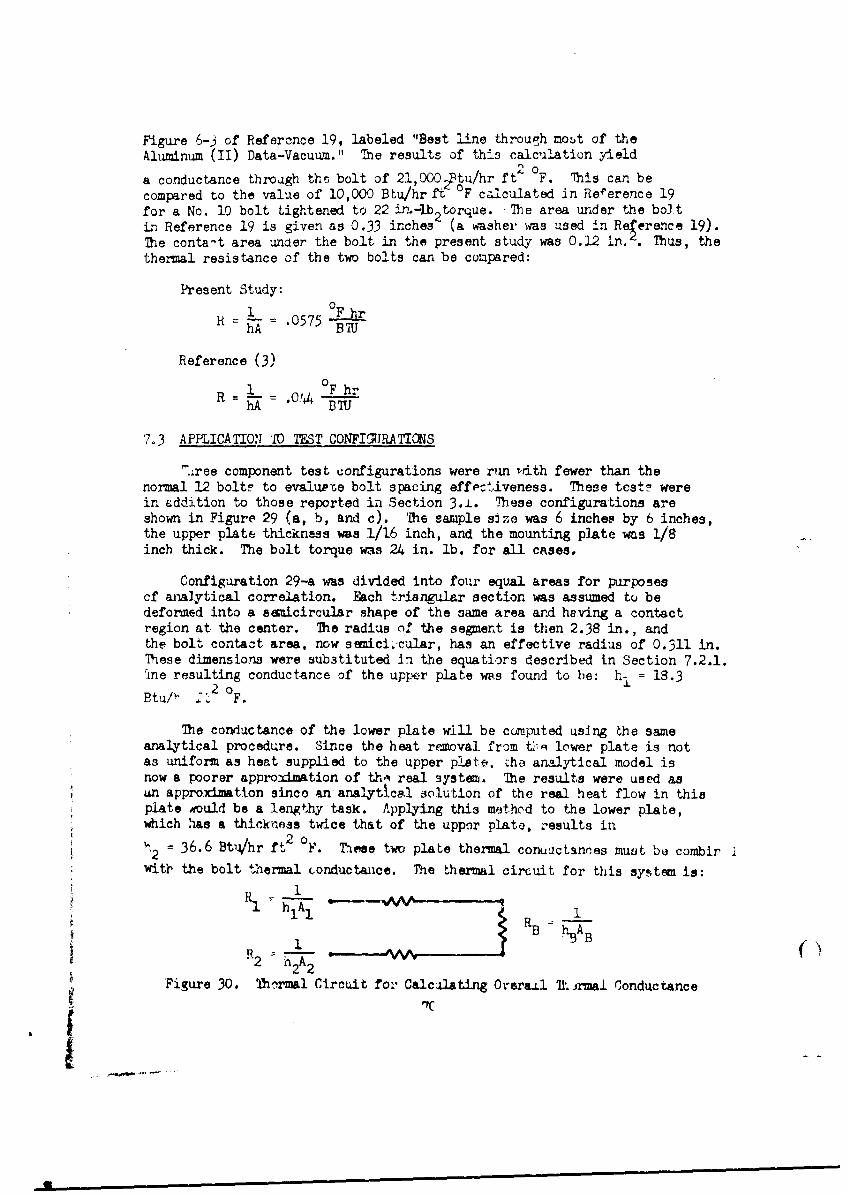
Figure 6-3 of Reference 19, labeled "Best line through most of theAluminum (II) Data-Vacuum." The results of thIs calculation yield

a conductance throagh the bolt of 21,O0002Btu/hr ft 2F. This can becompared to the value of 10,000 Btu/hr ft OF calculated in Reference 19for a No. 10 bolt tightened to 22 in.-lb2 torque. The area under the boltin Reference 19 is given as 0.33 inches (a washer was used in Reference 19).The conta-t area uncer the bolt in the present study was 0.12 iLn. 2 . Thus, thethermal resistance of the two bolts can be compared:

Present Study:

.0575 -F hr

hA B--h

Reference (3)

R 1 .0!41 0F hr

hA DIU

7-3 APPLICATION 10 TEST CONFIMJATIONS

7,ree component test configurations were rn .ith fewer than thenormal 12 boltr to evalupte bolt spacing effpetiveness. These tcst! werein addition to those reported in Section 3.1. These configurations areshown in Figure 29 (a, b, and c). 'he sample sjie was 6 inches by 6 inches,the upper plate thickness was 1/16 inch, and the mounting plate was 1/8inch thick. The bolt torque was 24 in. lb. for all cases.

Configuration 29-a was divided into four equal areas for purposescf analytical correlation. Each triangular section was assumed to bedeformed into a semicircular shape of the same area and having a contactregion at the center. The radius on the segment is then 2.38 in., andthe bolt contact area, now ssmci-cular, has an effective radius of 0.311 in.These dimensions were substituted in the equatiors described in Section 7.2.1.Tne resulting conductance of the upper plate was found to be: h i = 18.3

Btu/' 2 oF.

The conductance of the lower plate will be computed using the sameanalytical procedure. Since the heat removal from t> q lower plate is notas uniform as heat supplied to the upper plate, che analytical model isnow a poorer approximation of th% real system. The results were used asan approximation since an analytical solution of the real heat flow in thisplate aould be a lengthy task. Applying this method to the lower plate,which has a thickness twice that of the uppor plate, results in

2 = 36.6 BtA/hr ft 2 'F. These two plate thermal conuactances muot be combir i

witl the bolt thermal tonductance. The thermal circuit for this system is:

1

113

Figure 30. lhbrmal Circuit for Calc4Lating Or-erail Tirmal Conductance

.C

The overall conductance is given by:

1 _ 1 1 1-

hA A h2A2

Substituting the values gives:

1 _ 1 + i 3 6 .6hA 18.3 (9) 21,000 12 36.6

11.1 _ .874 + .057 + .437

or 12oh .1.7 Btu/hr ft F

1.3 68(e9

Applying this technique to Configuration 29-b, the corner bolts wereclose together and were lumped together to form a quarter circilar areahaving an effective radius of 0.622 inches. The analytical methodof Section 7.2.1 and thermal cirguit substitutions yield an overallconductance of h = 8.0 Btu/hr ft4 OF.

Configuration 29- wnj dividd by allotting to each corner bolt a

Shemicircular area of 4 in.- and each center bolt a quarter circle of 5 in.Using the same technique as above, the thermal circuit gave:

h = 22.0 Btu/hr ft' OF.

The twelve-bolt configuration was analyzed in the same manner by dividingthis area into eight equal area segmente as shown in Figure 29-d. Theresult was:

2 oh = 26.7 Btu/hr ft F.

The 6 inch by 12 inch component configuration can be approached usinghe same technique y dividing the area into eight hemici. .;alar sectors2

ad four quarter circular sectors each with an effective ar i of 6 inch2 .Sirilarly the 12 by 12 configuration ws dividid into twelve hemicirclesan four quarter circles of equal area, 9 inch'. The results for thesesix configurations are shown in Mble 8.

The 6 inch by 6 inch, 12 bolt and 12 inch by 12 inch, 24 boltconfigurationr can also be predicted using the method described inSection 7.2.2. An effective radius based on ths plate area ws used inEqation 7-li. The results are also given in Table 8. The results ofthese crrelation attempts are compmaw-wvo the sueasured values in Table 8.The agreement is adequate in all cases ecept 29-b -wheze the predictedvalue is a littI9 more -han half of the measured conductance. Ir. spite ofthis, the success of the technique is quite satisfactory. Firtherexploitation should b, mde of the approach described here. The resultshave been restricted to a bolted thizi plate without a filler material.

71

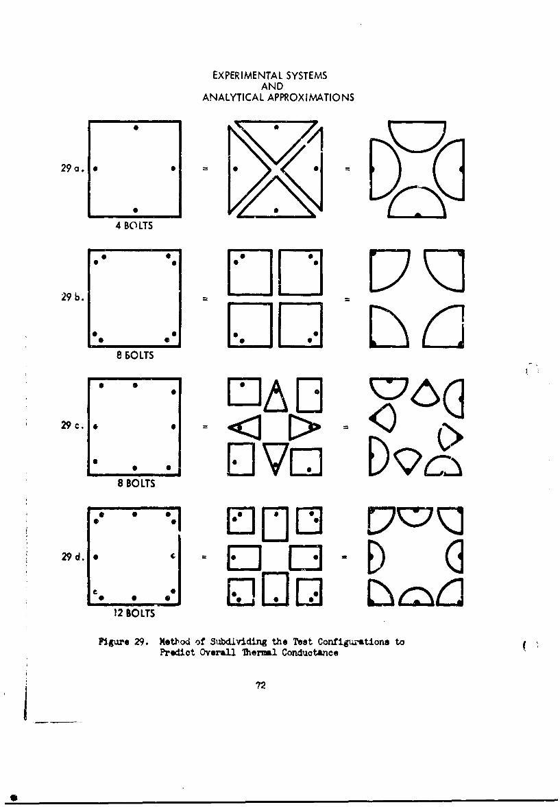
EXPERIMENTAL SYSTEMSAND

ANALYTICAL APPROXIMATIONS

29a. e = = 0 Q

4 BOLTS

29 b.

8 BOLTS

29c. >

8 BOLTS

0 0

•EJDE7KJ

2 BL TS

Fliure 29. Metbod of SubdiviLding the Test Configiztions toPreict OveraUl Thermal Conductance

72

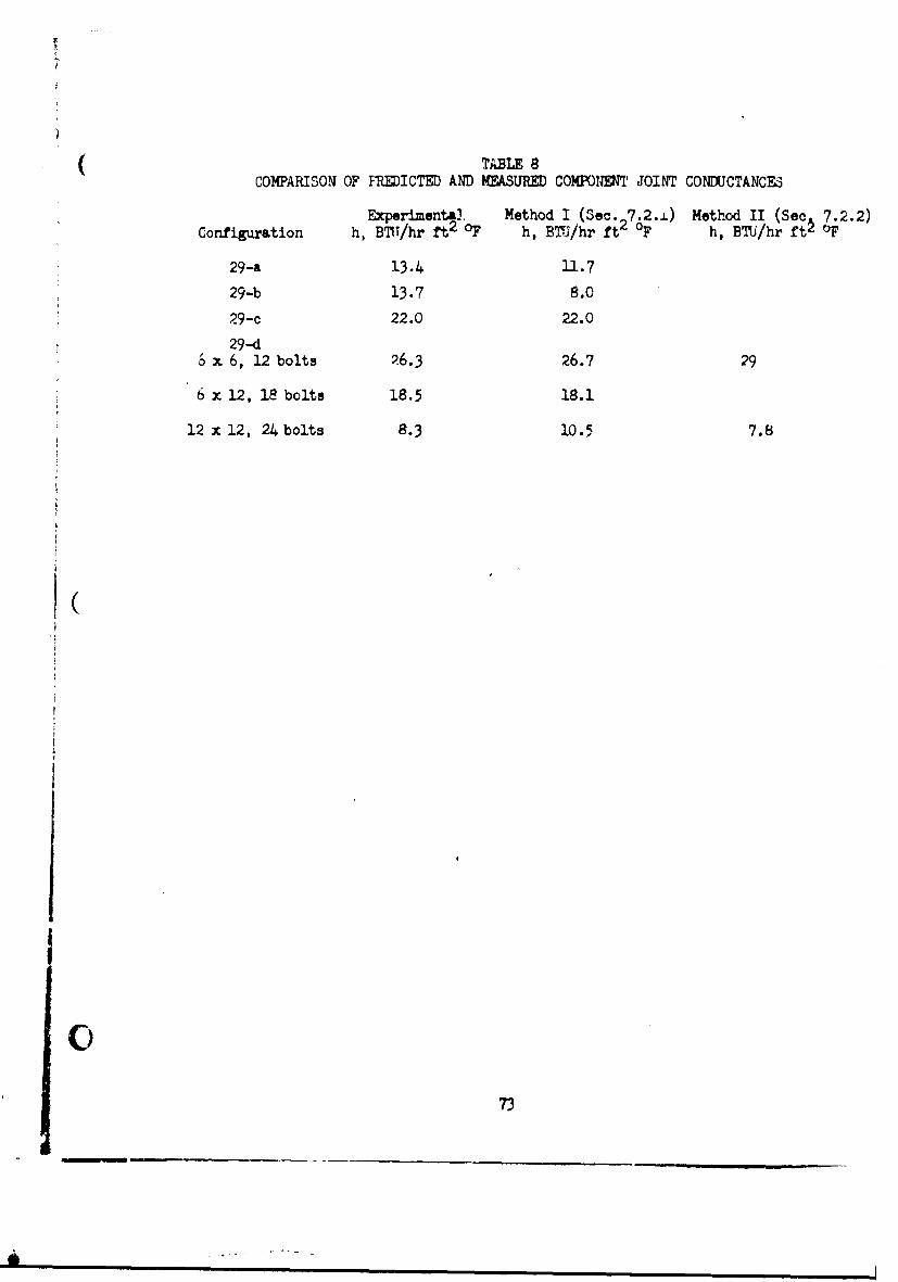
( TABLE 8COMPARISON OF FREDICTED AND MEASURED COKIYDOIENT JOINT CONDUCTANCES

Experimental, Method I (Sec. 7.2.1) Method II (SecA 7.2.2)Configuration h, BTIT/hr ft2 OF h, B7J/hr ft2 6F h, BTU/hr ftz OF

29-a 13.4 11.7

29-b 13.7 8.0

29-c 22.0 22.0

29-d6 x 6, 12 bolts 26.3 26.7 29

6 x 12, 18 bolts 18.5 18.1

12 x 12, 24 bolts 8.3 10.5 7.8

(

I

73

" - - - - - -

An attempt should be made to extendi this to thick plates withi an withouta filler andi to thin Plates with a filler.

I 74

8. CONCLUSIONS AD RECOMEATIONS

This report presents the results of the first phase of a programdesigned to improve the prediction of spacecraft thermal performance.The information necessary for the comparison of prediction and test of aspAcecraft model has been gathered. The continuation of the program to thisnatural conclusion is the second phase of the study. There has been nodecrease in the practical needs for this continuation and it is importantto complete this program.

There have been several developrentm within this program whichwarrant further study. The first is the extensiun of the joint conductancetesting to include a larger number of joint types. The techniques whichhave been developed in this program for experimentally measuring theconductance of practical joints have proven to be very simple and inexpensive.The accuracy which is obtained is adequate for such joints and is asatisfactory coupromise with the cost of such experimentation. The jointsfor this additional work should not be chosen on the basis of a thermal teatmodel but selected for the frequency with which they are used in actualpractice, e.g., riveted joints, low conductance joints, etc.

The practical correlation of joint conductances should also be continued.The correlation for the thin plate unfilled component joints was obtained byassuming the primry resistance to heat flow was in the thin plates. This

( primary resistance was found to be adequately described by radial in theregion surrounding each bolt fastener. The success with vhich the componentjoints were correlated by this procedure was very encouraging. The limitationsof time and resources did not allow a similar attempt to be made tocorrelate filled joints or structural joints. Aowever, such a correlationis believed to be feasible. This wort could be included in the second phaseof the progrem; correlation of other test joints would be performed as part ofthe experimental work d9secribed above or as a separate study. Regardless ofthe mechanism chosen for performing this correlation, this work should becontinued and extended.

The application of the directional specular-diffuse method of analysis hasindicated a major gap in our knowledge of thermal radiation properties. Acritical part of this method is the separation of the therval radiation proper-ties into the diffuse and specular coponents. Additional experimental ardanal.tical wort is required to develop a basis for this .epa"tion fromseLsurements of the directional and specular reflectance.. Such a st,4yshould include an exuination of the geometrioal reflectance. (arc aittance)relative to the distribution of reflected (and emtted) radiation.

jA lthoudI the camparisons of predicted and eerim ntal radiation exchangein the simple geometriese woere close, further refinement of the predictionsare desired. This prblem is related in part to the separation of the diffuseand specular compo;ncut discussed above. Tho efect of nin-g rv radiationproperties is probably of equal or greater importance. Purthr study i-needed for the improvement of the predicted tmgpersturee anW heat fluxm.,

C) e.g., a prediction using the band enera method.

75 _ _ __ _ _

In conclusion, the objectives of the first phase of the program havebeen satisfied; i.e., the data and methods required to compare thepredicted and test thermal performance of a model spacecraft have beendeveloped. Other areas for further study have also been found:

(1) practical Joint conductance measurements(2) correlation of measured joint conductances(3) t- separation of radiation properties into diffuse and

specular components for the directional specular-diffuseanalysis

,) the importance of the non-gray property assumption

The development of additional problems is to be expected in a study of thisnature. The second phase of the program should be expected to raise itsown share of new problems.

()76

I e

(REFMRICES

1. H. C. Hottel, "Radiant Heat Transmission," Chapter 4 of HeatTransmission, 3rd Ed., W. H. McAdams, McGraw-Hill Book Co., New York,1954.

2. B. Gebhart, "Unified Treatment for Thermal Radiation TransferProcesses," Paper No. 57-A-34, Winter Meeting AS.(E, Dec. 1959.

3. A. K. Oppenheim, Tras 78:725-735 (1956).4. J. T. Bevans and D. K. Edwards, "Radiation Exchange in an Enclosur-

with Directional Wall Properties," presented at the ASME WinterMeeting, Dec. 1965, Paper No. 64A/HT-52, published in theAugust issue of the Journal of Heat Tr&nsfer 87:388-396 (1965).

5. C. D. Coulbert and Chien Liu, W.DC TN 53-50 June 1953.6. T. Ishimoto and J. T. Be-ans, AIAA Journal 1:1428-9 (1963).7. E. M. Sparrow, "On the Calculation of Radiant interchange Between

Surfaces," pp 181-212, W. Ibele editor Academic Press, New York, 1963.8. J. T. Bevans and R. V. Dunkle, fans. ASME, Series C 82:1-19 (1960).9. E. M. Sparrow, et al., ke. A , Series C 84:294-299 (1962).10. D. K. Edwards and J. T. Bevans, "Effect of Polarization on Spacecraft

Radiation Heat Transfer," to be ptblished in the July issue of theAIAA Journal, 1965.

11. R. V. Dinkle, et al., "Heated Cavity Reflectometer for AngularReflectance Measurements," Prog. in Intl. Research on Thermcdyramics andTransport Properties Am. Soc. Mach. RWrs., pp 541-562 (1962).

12. A. M. Ciausing and B. T. Chao, "The:-=-_ Contact Resistance in a3 Vacuum Dvironment," University of Illinois Eperimental StationReport, NE-TN-242-1, August 1963.

13. H. Atkins, "Bibliography on Thermal Metallic Contact Conductance,"NASA TK X-53227, April 15, 1965, Marshall Space Flight Center.

14. H. Fenech and W. M. Rohserow, "Prediction of Thermal Conductance ofMetallic Surfaces in Contact," (Paper No. 62-4T-32)J. Heat Transfer, Vol. 85, pp 15-24, Feb,

15. J. J. Henry and H. Fenech, "The Use of Analogue Computers forDete:zmining Surface Parameters Required for Prediction of ThermalContact Zonductance," ASHE Paper 63-WA[-104, 1963; also J, of HeatTrAWer Transact4on of AW, Vol. 86, Series C, No. 4, Nov. 1964.

16. W. K. Aron and G. Colombo, "Controlling Factors of Thermal ConductanceAcross Bolted Joints in a Vacuum," ASM Paper 63-W-196.

17. K. G. Lindh, et al., "Studies in Heat renafer in Aircraft StructureJoL,ts," UCLA Report 57-50, My 1957.

18. J. . ile, n n, MeGrw "ill Book Co., Inc. New York, 1956.19. M. F. Blom, "Therm). Contact Conductance in a Vacuum &nvirorment,"

Douglas Aircraft Report SM-477O, Dec. 1964.

0

I I I I II|I II " : :- _ 7 7

APPENDICE5

I. Experimental Data-Component JointsII. Structural Joint Tests

III. Script F Comuter Program Print OutIV. Experimental Data-Radiation Exchange ExperimentV. Bibliogrst for Joint Therml Conductance

VI. Component Joint Test Data used for Correlation Task

78

APPENDIX I

EXPERIMENTAL DAsTA- COMPONENT JOINTS

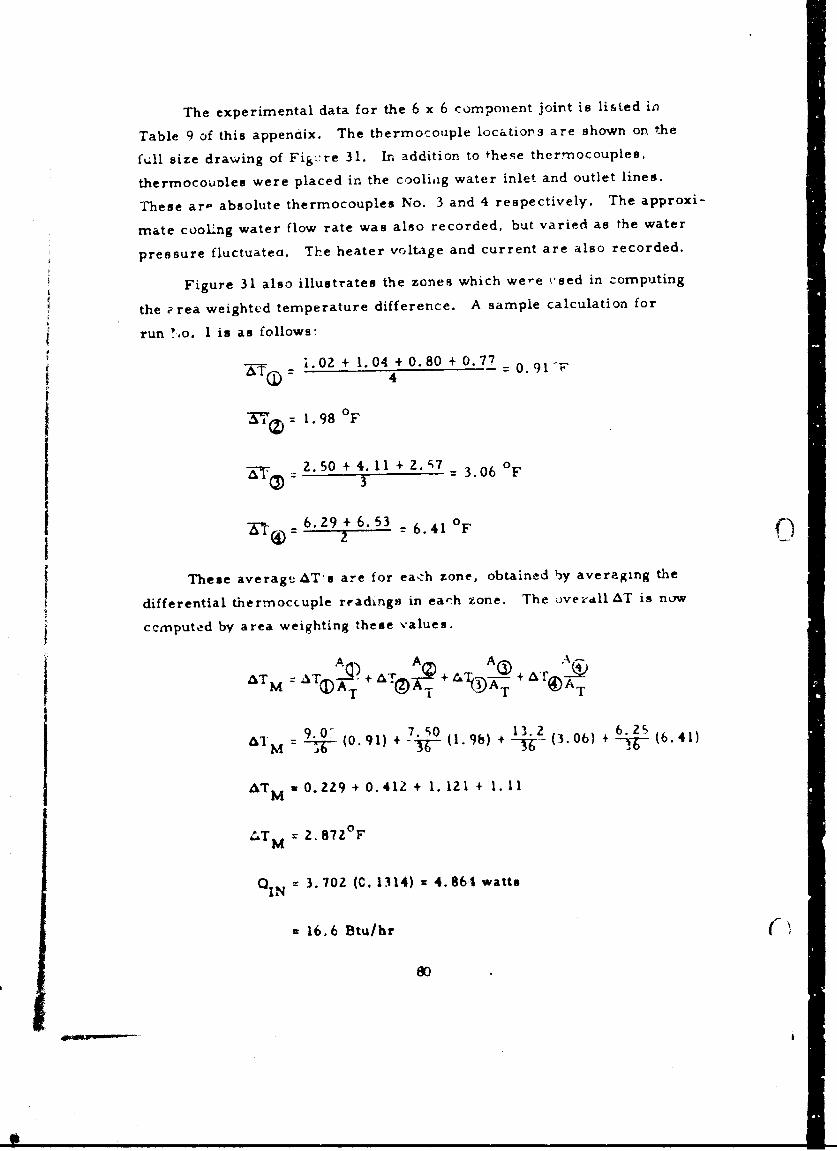
The experimental data for the 6 x 6 component joint is listed in

Table 9 of this appendix. The tbermocouple locatiors are shown on the

full size drawing of Figsvre 31. In addition to these thermocouples,

thermocouoles were placed in the cooliag water inlet and outlet lines.

These ar- absolute thermocouples No. 3 and 4 respectively. The approxi-

mate coollng water flow rate was also recorded, but varied as the water

pressure fluctuated. The heater voltage and current are also recorded.

Figure 31 also illustrates the zones which wee ised in computing

the -rea weighted temperature difference. A sample calculation for

run '.o. I is as follows:

1. 02 + 1"04+0. 80 +0. 77 = 0.91AD 4 0

-st ( 1. 98 °F

2.50 + 4. 1 +2.7 3.06

6. 29 + 6.53 = 6.41 0 F

These average AT's are for each zone, obtained 'y averaging the

differential thermoccuple rradings in earh zone. The uve-dll AT is now

ccnputed by area weighting these values.

A A A A

ATM= AT + A'r +~ +aT 4:

ATM =9. , (0.91) + - (1.9b) + 1-.2 (3.06) + 6 (6.41)

ATM = 0.229 + 0.412 + 1. 121 + 1. 11

LTM = 2. 872 0 F

QIN 3. 702 (C. 1314) - 4. 864 watts

16.6 Btu/hr ('

80

16.6 Btu/hr

2.8720F

s=23.1 Btu/b- ft 2 oI

The exrerimental data for he 6 inch x 12 inch an,- 12 inch x 12 inchcomponent Jcints are given in Tables 10 and li, respec'ively, ef this

appendix. The hernocouple locitions and temperature weighting zones

are .3hown in Figures 32 and 33 for these two experimental configarations.

Differential therraocouples are located at the eame (x, y) coordinates

on the back of the mounting plate and the component plate at the lucations

shown on FiSures 31, 32 and 33.

The conductance is calculated using the following eq'iation:

h Q

The area used in this cakculiticti is the contact area of the mating parts.

For the structural joints, this was the overLap area between the angle

bracket a nd the panel. rhe AT is an area weigLted averag- which is deter-

mined by the r.ethod explaired in above.

I

)8

_ _ _ _ _s ..

6.

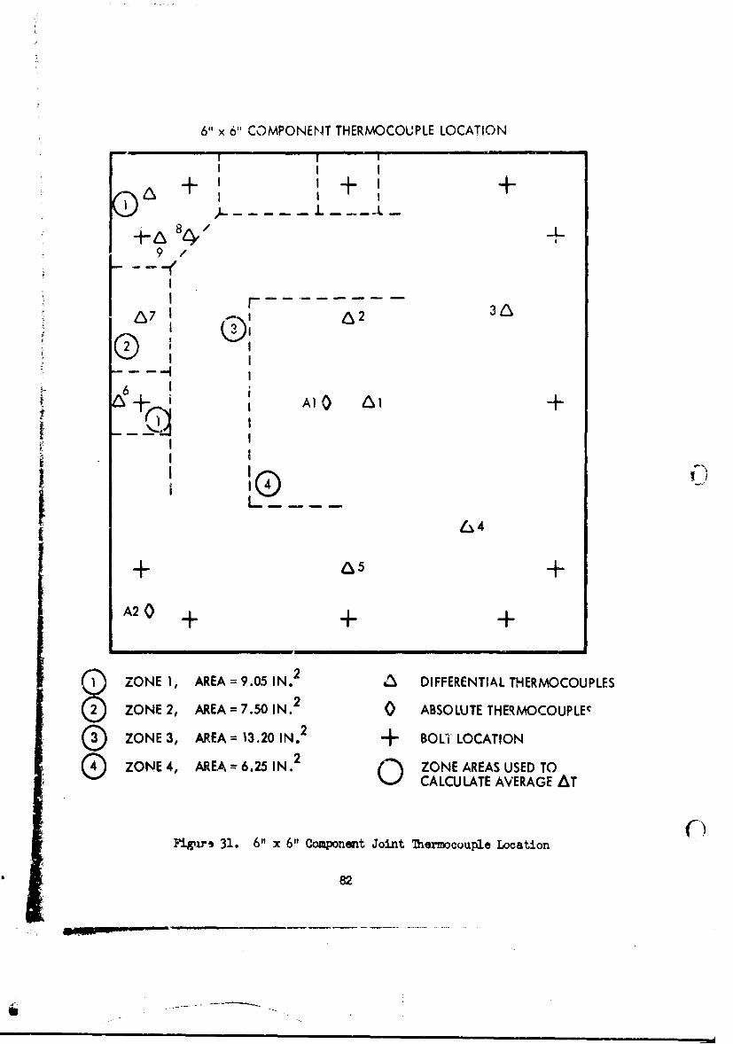
6" x 6" COMPONENT THERMOCOUPLE LOCATION

I I I

SI g

IL I-F:

9 /

A7 1 A2

0 0:$" I

6 + A10 I

i- -

4

A2 0 ,,- ++

ZONE 1, AREA =9.05 N. 2 DIFFERENTIAL THERMOCOUPLES

( ZONE 2, AREA = 7.50 IN. 2 0 ABSOLUTE THERMOCOUPLEc

ZONE 3, AREA =13.20 IN. 2 + BOLT LOCATION

() ZONE 4, AREA 6.25 IN. 2 ZONE AREAS USED TO0 CALCULATE AVERAGE AT

Fiurs 31. 6" x 6" Component Joint Thermocouple Location

82

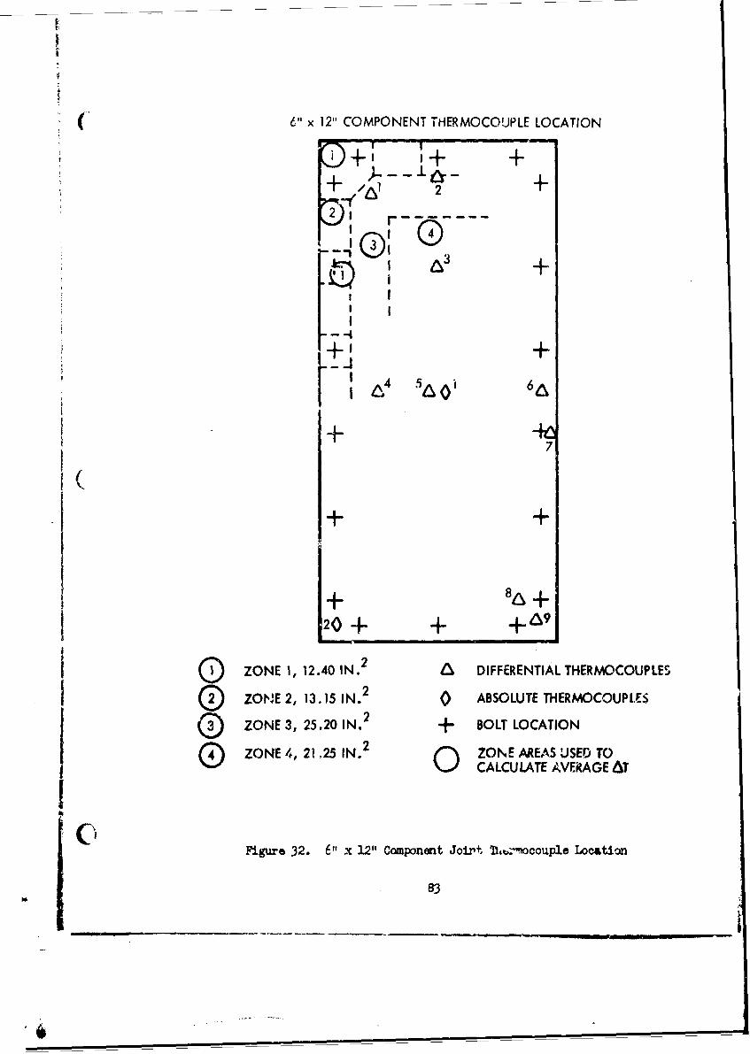
I

6"x 12" COMPONENT THERMOCOUPLE LOCATION

1+, 1+ +++2J' r

I

L, +I6 4 5 oj 66X

-1- 7

+ 8&x +120 + +69

ZONE 1, 12.40 IN. 2 DIFFERENTIAL THERMOCOUPLES

ZONE 2, 13.15 IN. 2 0 ABSOLUTE THERMOCOUPLES

ZONE 3, 25.20 IN. 2 + BOLT LOCATION

ZONE 4, 2125 IN. 2 ZONE AREAS USED TOCALCULATE AVERAGEAT

~clFigure 32. 6" x 12" Component Joir+t 2, -couple Location

83

i 4

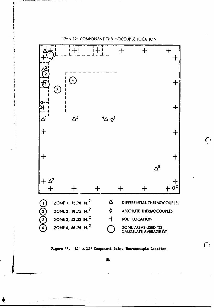
'I12" x 12" COMPONENT THEE 'AOCOUPLE LOCATION

[Q2 -- -- -- - +

+ + +I+

N- +

I +

A' +

Ci

A8

+ + + + + o2

ZONE 1, 15.78 IN. 2 A DIFFERENTIAL THERMOCOUPLES

ZONE 2, 18.75 IN. 2 0 ABSOLUTE THERMOCOUPLES

) ZONE 3, 53.22 IN. 2 + BOLT LOCATION

ZONE 4, 56.25IN.2 ZONE AREAS USED TOG 0 CALCULATE AVERAGE AT

Figure 33. 12" x 12" Component Joint Thermocouple Location

84

I

Table 9. Experimental Data-6 by 6 Inch Cornjoncnt Joints

Run No. 1 2 3 4 5

Date 10/26/64 10/26/64 10/26/b4 i0/26/64 10/27/64

Pressure, Torr 6 x 10 7 6 x 10 7 6 x 10 7 6 x 10 7 5 x 10 - 7

Absolute T. C.

1 - °F 85.7 95.3 107.1 119.0 85.32 - °F 80.2 85.6 91.0o 97.8 79.83 - 0F 74.0 74.5 74.5 74.3 73.8

4 - oF 74.1 74.8 75.0 75.0 74.0

Differential T. C.

1 0 F 6.53 11.78 18.28 24.72 6.722 - F 6.29 11.38 17.60 23.78 6.48

3 - F 2.50 4.56 7.25 9.85 2.524 - °F 4.11 7.06 10.95 14.90 4.055 - °F 2.57 4.64 7.25 9.81 2.63

6 - OF 1.02 1.81 2.81 3.81 1.027 - °F 1.98 3.52 5.46 7.40 2.00

8 - °F 1.04 1.88 2.92 3.96 1.07

9 - 0F 0.80 1.41 2.19 2.97 0.81

10 - 0 F 0.77 1.31 2.04 2.77 0.74

Voltage., volts 37.02 49.31 61.54 72.04 36.99

Current, amps 0. 1314 0. 1750 0.2185 0.2560 0. 1313

Water Flow, ml/min 725 650 650 650 575

Bolt Torque, in-lb 24 24 24 24 24

Filler "4one None None None None

Sample Number I I I I I

Number of Bolt* 12 12 12 12 12

h, Btu/hr ft2 or 23.1 22.9 23.0 22.3 22.8

_. n85

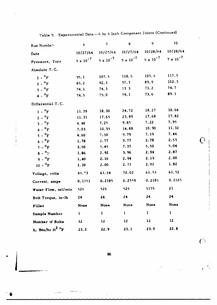
Table 9. Experimental Data- 6 by 6 Inch Component Joints (Continued)

Run Ntunbc:' b 7 8 9 10

Date 10(27/64 10127/64 10/27/64 10/28/64 10/28/64

Pressure, Torr 5 x 10 - 7 5 x 107 5 x 10 - 7 6 x 10 - 7 7 x 10 - 7

Absolute T. C.

I - 0F 95.1 107.5 118.5 105.5 117.5

2 - OF 85.2 92.3 97.3 89.9 102.3

3 - OF 74.1 74.3 73 3 73.2 74.7

4 - 0 74.5 75.0 74.1 73.6 89. 1

Differential T. C.

1 - 0F 11.78 18.30 24.72 18.27 18.68

z - OF 11.31 17.65 23.89 17.68 17.82

3 - 0F 4.48 7.25 9.85 7.22 7.95

4- 0 F 7.03 10.95 14.88 10.90 11.32

5 - F 4.60 7.50 9.79 7.19 7.44

6- OF 1.78 2.77 3.77 2.78 2.53 417 - 0 F 3.50 5.45 7.37 5.50 5.04

8 - v, 1.86 2.92 3.96 2.94 2.87

9 - F 1.40 2.16 2.94 2. 19 2.00

10 - 0 1.30 2.00 2.71 2.02 1.82

Voltage, volts 49. '3 61.54 72.02 61.53 61.52

Current, amps 0.1751 0.2185 0.2559 0.2185 0.2165

Water Flow, mllr in 525 525 525 1175 21

Bolt Torque. in-lb 24 24 24 24 24

Filler None None None None None

Sample Nuznber 1I I I I

Number of Bolts 12 12 12 12 12

h. Btu/hr ft 2 °F 23.2 22.9 23.1 23.0 22.8

86

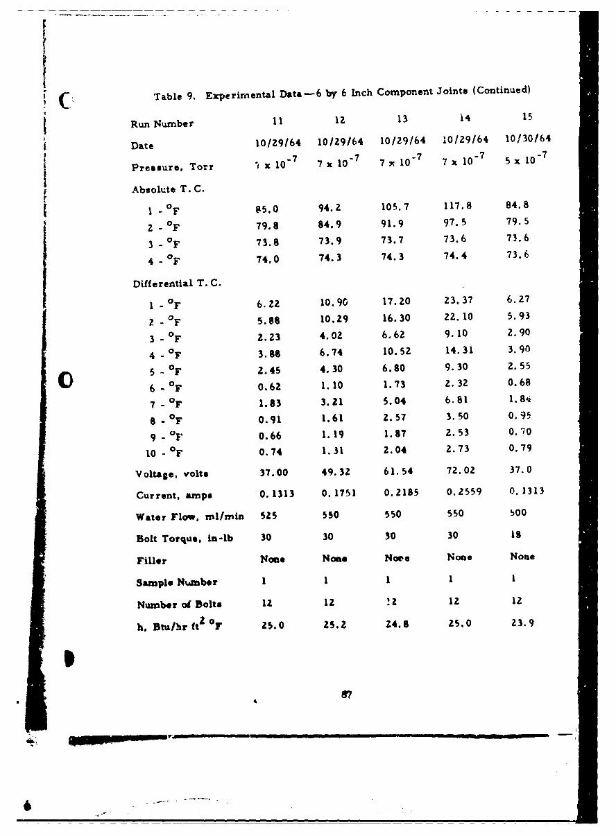
I (Table 9. Experimental Data-6 by 6 Inch Component Joints (Continued)

Run Number 11 lz 13 14 15

Date I0/Z9/64 10/29/64 10/29/64 !0/29/64 10/30/64

Pressure, Torr 'I x 10 7 7 x 10 7 7 10 7 7 x 10 7 5x 10-7

f Absolute T. C.

I - 0F 85.0 94.2 105.7 117.8 84.8

2 - 0F 79.8 84.9 91.9 97.5 79.5

3 - 0 F 73.8 73.9 73.7 73.6 73.6

4 - 0 F 74.0 74.3 74.3 74.4 73.6

Differential T. C.

1 - 0 F 6,2 10.90 17.20 Z3.37 6.27

? - F .88 10.29 16.30 22.10 5.93

3 - .F 2.23 4.02 6.62 9.10 2.90

4 - 0 F 3.88 6.74 10.5Z 14.31 3.90

5 - 0 F 2.45 4.30 6.80 9.30 2.55

6 - °F 0.62 1.10 1.73 2.3Z 0.68

7 - OF 1.83 3.21 5.04 6.81 1.8,1

8 - °F 0.91 1.61 2.57 3.50 0.95

9 - aF 0.66 1.19 1.87 2.53 0.70

10 - OF 0.74 1.31 2.04 2.73 0.79

Voltage, volts 37.00 49.32 61.54 72.02 37.0

Current, amps 0. 1313 0.1751 0.2185 0.2559 0. 1313

Water Flow, ml/min 5Z5 550 550 550 b00

Bolt Torque. in-lb 30 30 30 30 18

FiUer None None Noe None None

Sample Number 11 1 1 1

Number oBolts 1z 12 !Z 12 IZ

h. Btu/hr ft2 °F 25.0 ZS.Z Z4.8 2S.0 23.9

87

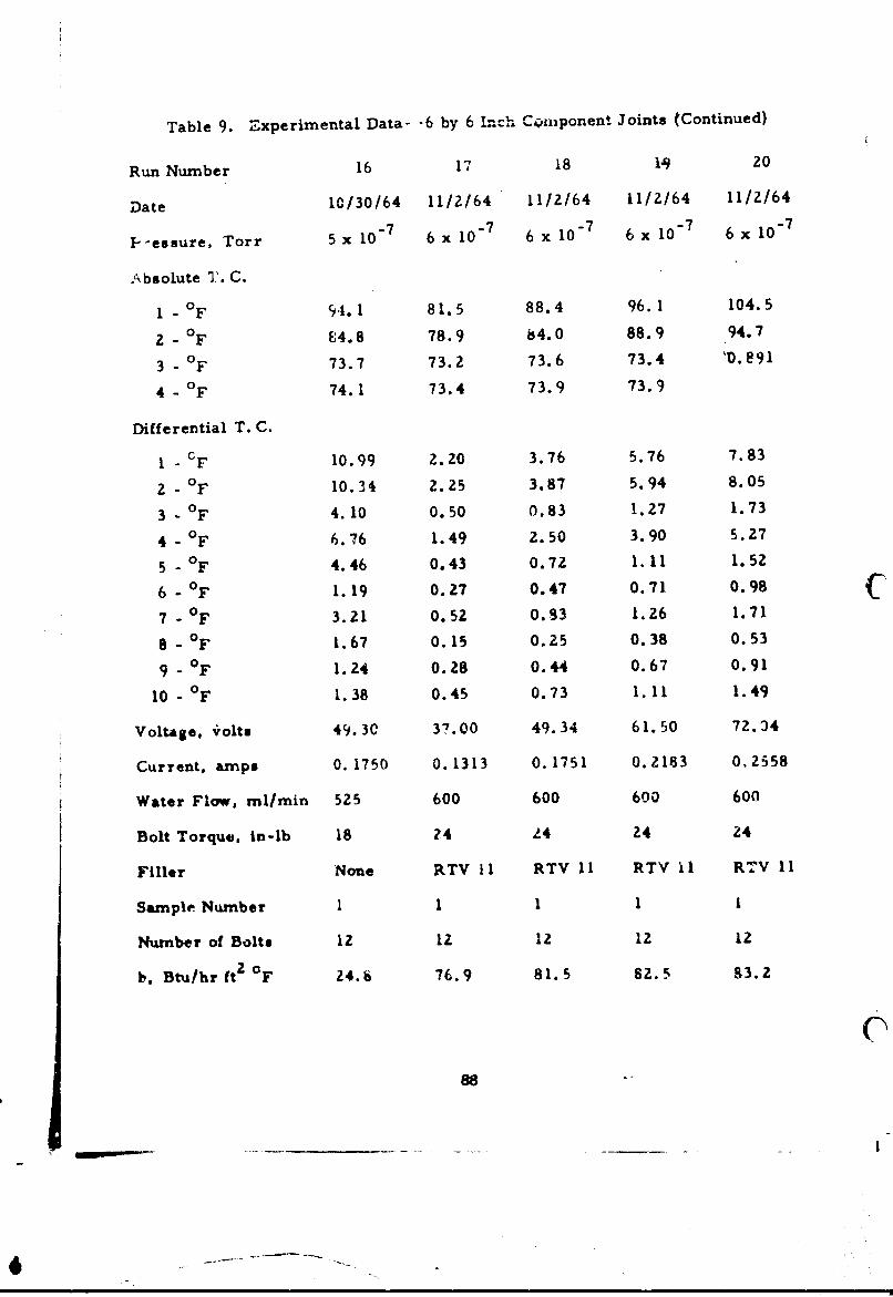
Table 9. Experimental Data- -6 by 6 Lnch Cwnponent Joints (Continued)

Run Number 16 17 18 1'q 20

Date 10/30/64 11/2/64 11/2/64 11/2/64 11/2/64

P-essure, Torr 5x 10 7 7 x6 x 10- 7 6 x 10 - 7 6 x 10 7

Absolute T. C.

1- 4F 9'. 1 81.5 88.4 96.1 104.5

2 - °F 64.8 78.9 84.0 88.9 94.7

3- 0F 73.7 73.2 73.6 73.4 10.891

4- 0 F 74.1 73.4 73.9 73.9

Differential T. C.

1 - F 10.99 2.20 3.76 5.76 7.83

2 - F 10.34 2.25 3.87 5.94 8.05

3 0 F 4.10 0.50 0.83 1.27 1.73

4 0 F 6.76 1.49 2.50 3.90 5.27

5- 0F 4.46 0.43 0.72 1.11 1.52

6 -F 1.19 0.27 0.47 0.71 0.98

7 - OF 3.21 0.52 0.83 1.26 1.71

8 - F 1.67 0.15 0.25 0.38 0.53

9- 0 F 1.24 0.28 0.44 0.67 0.91

10- 0 F 1.38 0.45 0.73 1.11 1.49

Voltage, volts 49.30 37.00 49.34 61.50 72.34

Current, amps 0. 1750 0.1313 0.1751 0.2183 0.2558

Water Flow, ml/min 525 600 600 600 600

Bolt Torque. in-lb 18 24 Z4 24 24

Filler None RTV I I RTV 11 RTV I I RTV I I

Sample Number 1 1 1 1 1

Number of Bolts iz 12 12 12 12

b. Btu/hr ft 2 oF 24.b 76.9 81.5 82.5 83.2

88

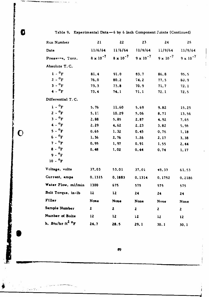
C Table 9. Experimental Data-6 by 6 Inch Component Joints (Continued)

Run Namber 21 22 23 24 25

Date 1116164 11/6/64 11/9/64 11/9/64 1119/64

Press,-i, Torr. 8 x 10 - 7 8 x 10 7 9 x 10 7 9 x 10 7 9 x 10 7

Absolvte T. C.

1 - 0 F 81.4 91.0 83.7 86.8 95.5

2 - 0F 76.0 80.2 74. 2 77.5 80.9

3 - oF 73.3 73.8 70.9 71.7 72.14 - 0F 73.4 74.1 71.1 72.1 72.5

Differential T. C.I - 0OF 5.76 11.60 5.69 9.82 15.25

S2 - 0°F 5.1I, 10.2Z9 5.06 8.71 13.56

3 - 0 F 2.88 5.85 2.87 4.92 7.65

4 - 0 F 2.29 4.62 2.23 3.82 5.96

5 - 0 F o.65 1.32 0.45 0.76 1.186 - OF 1.36 2.76 1. Z6 2.17 3.387 - oF 0.95 1.97 0.91 1.55 2.44

8 - 0 F 0.48 1.02 0.44 0.74 1.179 0 °F

10 0 OF

Voltage, volts 37.03 53.01 37.01 49.33 61.53

Current, amps 0.1315 0.1883 0.1314 0.1752 0. Z186

Water Flow, ml/min 1300 675 575 575 575

Bolt Torque, in-lb 12 12 24 24 24

Filler None None None None None

Sample Number 2 2 2 2 2

Number of Bolts 12 12 12 it 12

h. Btu/hr ft oF 24.7 2S.5 29.1 30.1 30.1

89

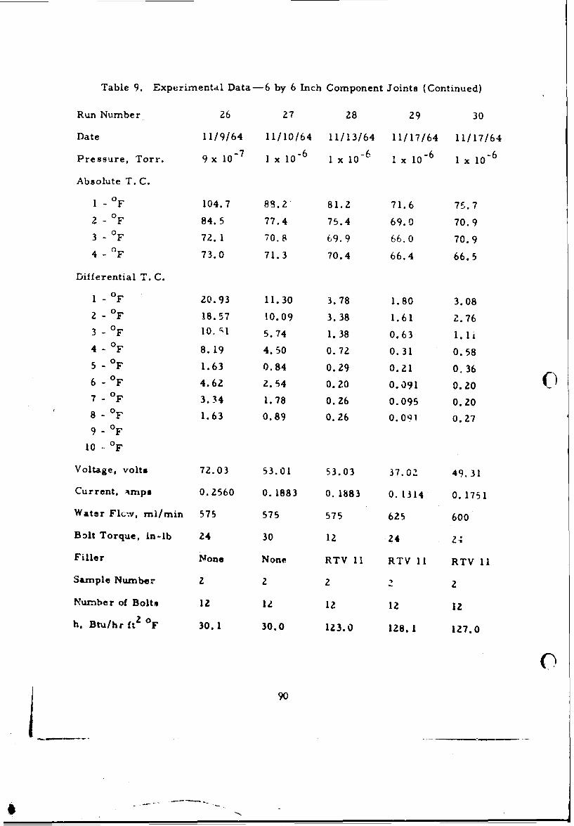
Table 9. Experimental Data-6 by 6 Inch Component Joints (Continued)

Run Number 26 27 28 29 30

Date 11/9/64 11/10/64 11/13/64 11/17/64 11/17/64

Pressure, Torr. 9 x 10 - I x 10 6 x 10-6 I x 10 - 6 I x 10 -

Absolute T. C.

I - °F 104.7 88.2' 81.2 71.6 75.7

2 - 0 F 84.5 77.4 75.4 69.0 70.93 - 0 F 72.1 70.8 69.9 66.0 70.94 - (F 73.0 71.3 70.4 66.4 66.5

Differential T. C.

1 - 0 F 20.93 11.30 3.78 1.80 3.082 - 0 F 18.57 10.09 3.38 1.61 2.763 - 0 F 10.51 5.74 1.38 0.63 1.1i4 - 0 F 8.19 4.50 0.72 0.31 0.585 - 0 F 1.63 0.84 0.29 0.21 0.366 -0 F 4.62 2.54 0.20 0.091 0.207 - 0F 3.34 1.78 0.26 0.095 0.208 - 0F 1.63 0.89 0.26 0.091 0.279 0 OF

10 OF

Voltage, volts 72.03 53.01 53.03 37.02 49.31

Current, %mps 0.2560 0. 1883 0. 1883 0. 1314 0.1751

Water F1l;v, mi/min 575 575 575 625 600

Bolt Torque, in-lb 24 30 12 24 2;

Filler None None RTV 11 RTV 11 RTV II

Sample Number 2 2 2 2 2

Number of Bolts 12 it 12 12 12

h, Btu/hr ft 2 OF 30.1 30.0 123.0 128.1 127.0

90

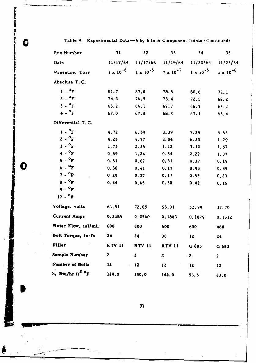
II

ID Table 9. Experimeontal Data-6 by 6 Inch Component Joints (Continued)

j Run Number 31 32 33 34 35

Date 11/17/64 11/17/64 11/19/64 11/20/64 11/23/6411 lxl 6 7x0 i 6 -6

Pressure, Torr I x 10 1 x 10 6 7 x 10 . 7 1 x 10- 1 x I0 -

Absolute T. C.

I - 0F 81.7 87.0 78.8 80.6 72.12 - OF 74.2 76.5 73.4 72.5 68.2

3 - 0 F 66.2 66.1 67.7 66.7 65.24 - OF 67.0 67.0 68.? 67. 1 65.4

Differential T. C.

1 - 0 F 4.72 6.39 3.39 7.25 3.62

2 - 0 F 4.25 5.77 3.04 6.20 1.293 - 0 F 1.73 2.35 1.1Z 3.lZ 1.574 - OF 0.89 1.24 0.54 2.22 1.07

5 - OF 0.51 0.67 0.31 0.37 0.19S6 - OF 0.30 0.41 0.17 0.93 0.45

7 - OF 0.29 0.37 0.17 0.53 0.23

8 - oF 0.44 0.65 0.30 0.42 0.159 0 oF

10 - F

Voltage, volts 61.51 72.05 53.01 5Z.99 37.C)

Current Amps 0.2185 0.2560 0.1883 0.1879 0.1312

Water Flow, wl/mL- 600 600 600 600 460

Bolt Torque, in-lb 24 24 30 1z 24

FMer IT 11 RTV 11 RTV 11 G 683 G 683

Sample Number 22 2 z

Number of Bolta lZ 12 12 12 lz

h. Btu/hr ft2 oF 129.0 130.0 142.0 55.5 63.0

91

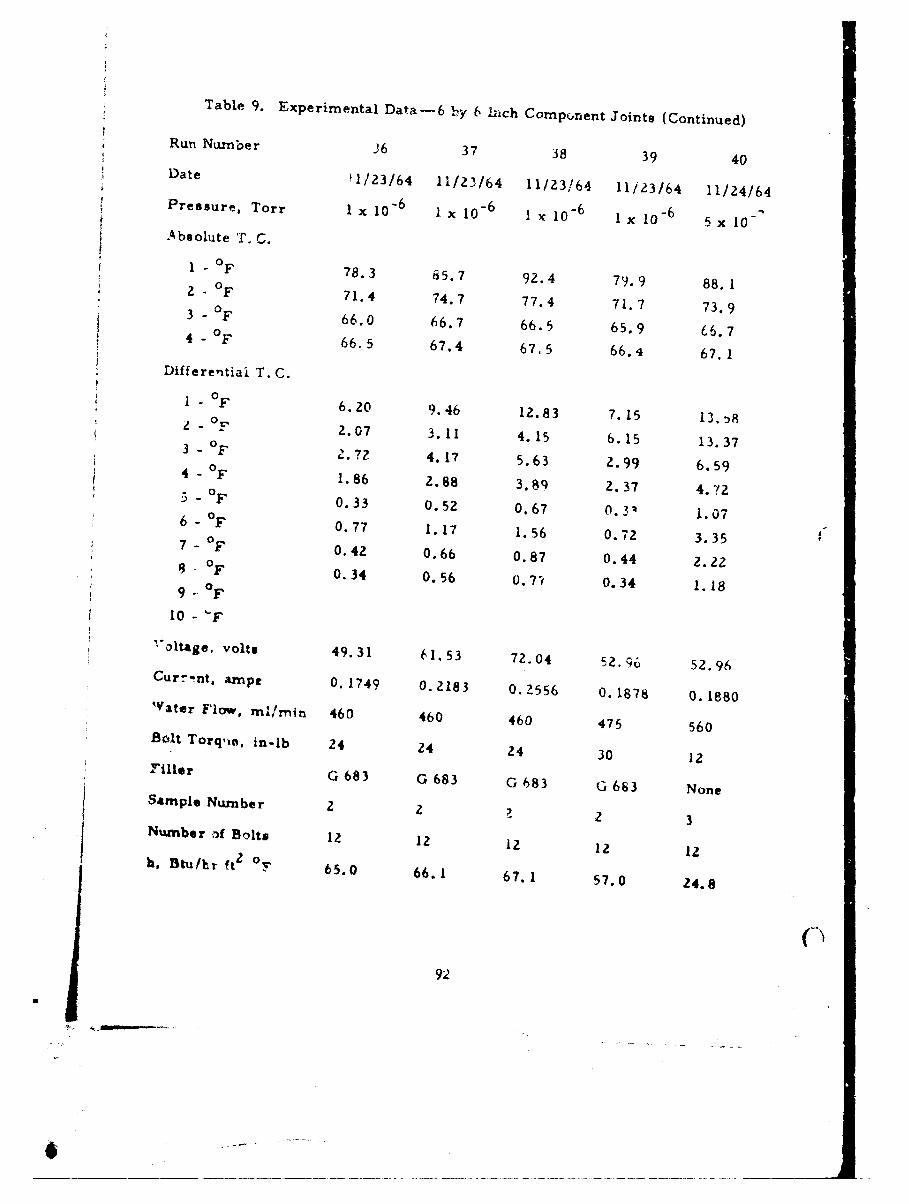
Table 9. Experimental Data-6 by 6 1hch Component Joints (Continued)

Run Number 26 37 38 39 40Date '1/23/64 11/23/64 11/23164 11/23/64 11/24164Pressure, Torr I x -6

Ix 10 6 x 10-6 5 x 10-'Absolute r. C.

1 - 0 F 78.3 65.7 92.4 79.9 88,12 °F 71.4 74.7 77.4 71.7 73.93 - 0F 66.0 66.7 66.5 65.9 66.74 - °F 66.5 67.4 67.5 66.4 67.1

Differentiai T. C.

1 F 6.20 9.46 12.83 7.15 13. !82 2.07 3.11 4.15 6.15 13.373 - 2.7? 4.17 5.63 2.99 6.594 - 1.86 2.88 3.89 2.37 4.72- F 0.33 0.52 0.67 0.31 1.076- OF 0.77 1.17 1.56 0.72 3.357- 0F 0.42 0.66 0.87 0.44 2.22

F 0.34 0.56 0.77 0.34 1.1809 F

i 10 -"F

'Oltage, volts 49.31 61.53 72.04 52.96 52.96Curr.nt, ampz 0.1749 0.2183 0.2556 0.1878 0.1880Water Flow, mi/rnin 460 460 460 475 560B0lt Torqic. in-lb 24 24 24 30 12

Filler G 683 G 683 G 683 G 663 NoneSample Number 2 2 2 3Nuzmber of Bolts 12 12 12 12 12h. Btu/,r ft o 65.0 66.1 67.1 57.0 24.8

U9

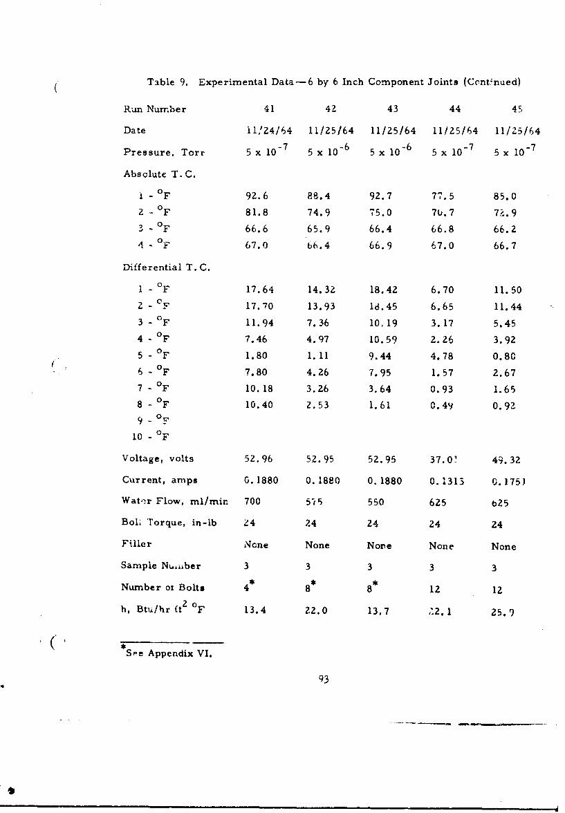
Table 9. Experimental Data-6 by 6 Inch Component Joints (Cont~nued)

Run Number 41 42 43 44 45

Date il/24/64 11/25/64 11/25/64 11/25/64 11/25/64

Pressure, Torr 5 x 10 5 7 5 x 16 x 10 - 6 5 x 10 - 7 5x 10- 7

Absolute T. C.

i - F 92.6 88.4 92.7 77.5 85.0

2 0 F 81.8 74.9 75.0 7U.7 7.9

3- °F 66.6 65.9 66.4 66.8 66.2

4 - OF 67.0 66.4 66.9 67.0 66.7

Differential T. C.

1 - °F 17.64 14.32 18.42 6.70 11.50

2 - oF 17.70 13.93 18.45 6.65 11.44

3 - 0 F 11.94 7.36 10019 3.17 5.45

4 - 0 F 7.46 4.97 10.59 2.26 3.92

5 - OF 1.80 1. 11 9.44 4.78 0.80

6 - 0 F 7.80 4.26 7.95 1.57 2.67

7 - F 0.18 3.26 3.64 0.93 1.65

8 - 0F 10.40 2.53 1.61 0.49 0.92

9 - V

10 - F

Voltage, volts 52.96 52.95 52.95 37.0' 49.32

Current, amps 0. 1880 0. 1880 0. 1880 0. 1313 0. 175)

Wat,;r Flow, ml/min 700 575 550 625 625

Bolt Torque, in-lb ;4 24 24 24 24

Filler Ncne None None None None

Sample Nuiiber 3 3 3 3 3

Number ot Bolts 4* 8* 8* 12 12

h, Btu/hr ft 2 oF 13.4 22.0 13.7 .2. 1 25.9

Spe Appendix VI.

93

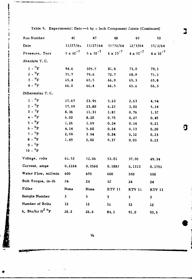
Table 9. Experimental Data-6 by o Inch Component Joints (Continued)

Run Number 46 47 48 49 50

Date 11/27/6- 11/27/64 111/30/64 12/3/64 1ZI 3/64-7 7 -7

Pressure, Torr 5 x 10 5 x 10 - 6 x 10 4 x 110 4 x 10

Absolute T.C.

01 - F 94.6 105.5 81.8 73.0 79.1

2 - °F 75.7 79.6 72.7 68.A 71.53 - 0F 65.4 65.5 66.0 65.3 65.8

4 - OF 66.0 66.4 66.5 65.6 66.3

Differential T. C.

0 0 F 17.67 23.95 5.63 2.63 4.54

- 17.59 23.80 6.21 3.00 5.14

3 F 8.36 11.31 -1.8! 0.76 1.32- 0 F 6.02 8.20 0.75 0.27 0.45

5 - °F 1.26 1.69 0.24 0.14 0.216 - OF 4.14 5.60 0.24 0.13 0.20

7 - OF 2.59 3.54 0.24 0.12 0.238 - 0 F 1.49 2.02 0.37 0.05 0.239 -OF!o0 F

Voltage, volts 61.52 72.06 53.01 37.00 49.34

Current, amps 0.2134 0.2560 0.1881 0.1313 0.1751

Water Flow, ml/min 600 600 600 550 550

Bolt Torque, in-lb 24 24 12 24 24

Filler None None RTV 11 RTV 1i RTV 11

Sample Number 3 3 3 3 3

Number of Boltd 12 12 lz 12 12

h, Btu/hr ft 2 OF 26.2 26.6 84.1 91.0 93.5

94

- li..._._____ -_i_______i__-,,.

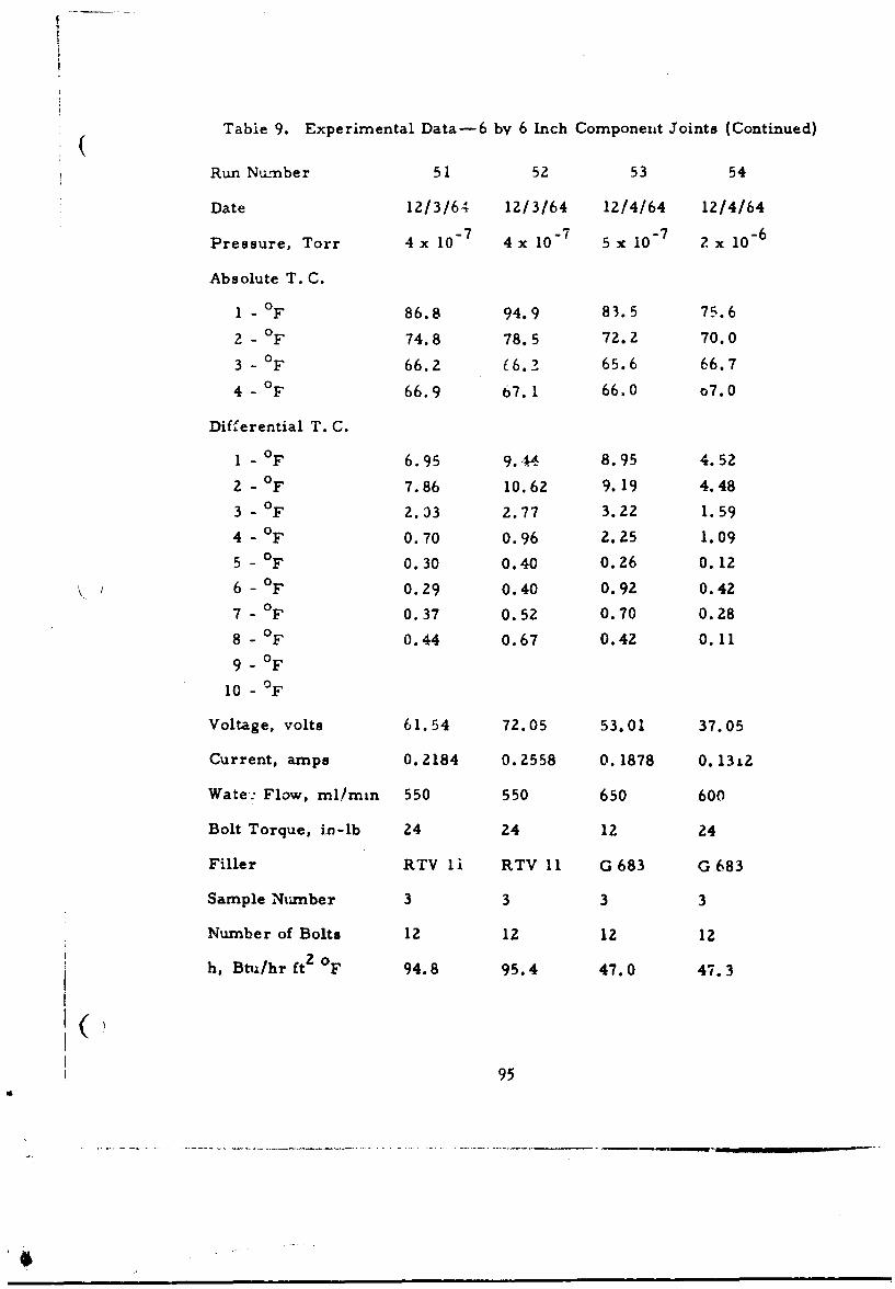
I

Table 9. Experimental Data-6 by 6 Inch Component Joints (Continued)

Run Number 51 52 53 54

Date 12/3/64 12/3/64 12/4/64 12/4/64

Pressure, Torr 4 x 10 - 7 4 x 10- 7 5 x 10- 7 2 x 10 - 6

Absolute T. C.

I - 0 F 86.8 94.9 83.5 75.6

2 - OF 74.8 78.5 72.2 70.0

3 - OF 66.2 (6.2 65.6 66.7

4 - 0 F 66.9 67.1 66.0 07.0

Differential T. C.

1 - 0 F 6.95 9.4 8.95 4.52

2 - 0F 7.86 10.62 9.19 4.48

3 - OF 2.33 2.77 3.22 1.59

4 - 0F 0.70 0.96 2.25 1.09

5 - °F 0.30 0.40 0.26 0.12

6 - OF 0.29 0.40 0.92 0.42

7 - 0F 0.37 0.52 0.70 0.28

8 - 0 F 0.44 0.67 0.42 0.119 0 OF

10 0 OF

Voltage, volts 61.54 72.05 53.01 37.05

Current, amps 0.2184 0.2558 0.1878 0.13,2

Wate: Flow, ml/mnn 550 550 650 600

Bolt Torque, in-lb 24 24 12 24

Filler RTV Ii RTV 11 G 683 G 683

Sample Number 3 3 3 3

Number of Bolts 12 12 12 12

h, Btu/hr ft 2 OF 94.8 95.4 47.0 47.3

95

--S

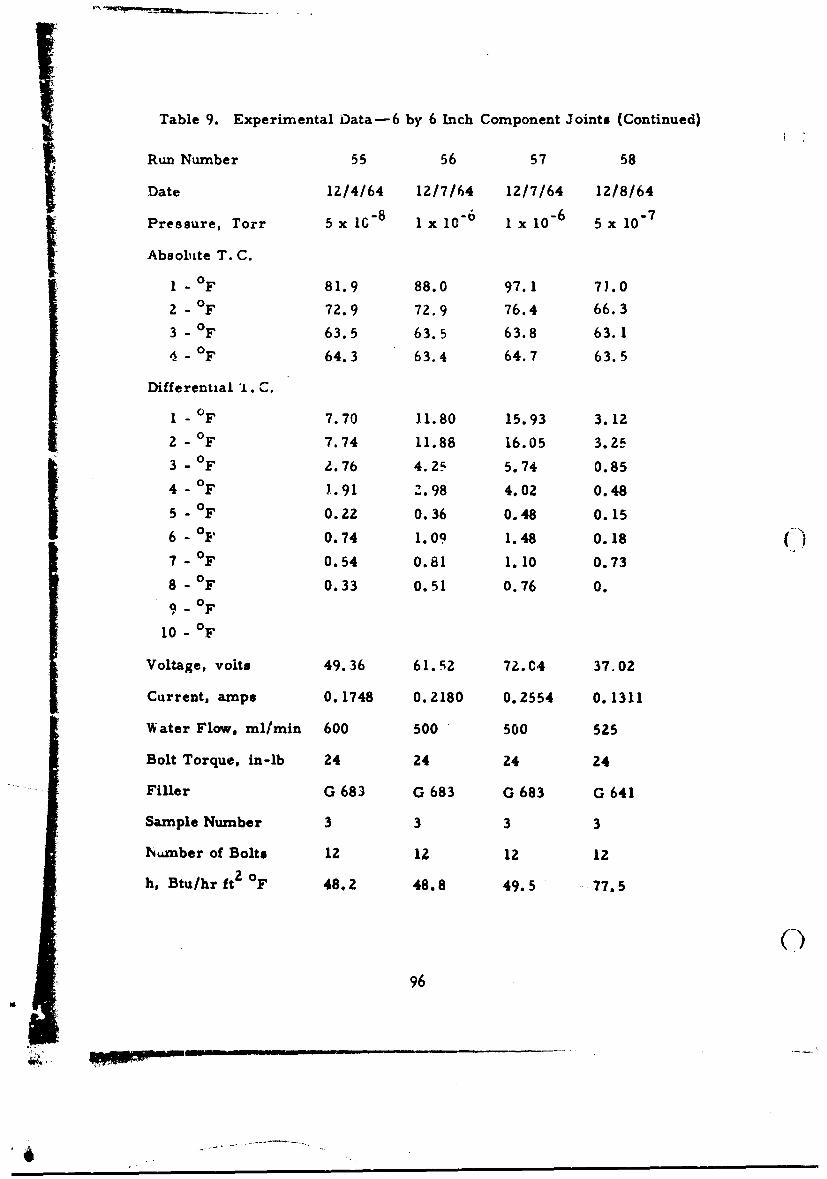
Table 9. Experimental Data-6 by 6 Inch Component Joints (Continued)

Run Number 55 56 57 58

Date 12/4/64 12/7/64 12/7/64 12/8/64SPressure, Torr 5 x IC 8 1 x 10- 6 1 x 10 - 6 5 x 10 7

Absolite T. C.

1 - 0F 81.9 88.0 97.1 71.0

2 - 0F 72.9 72.9 76.4 66.3

3 - OF 63.5 63.5 63.8 63.1

4 - OF 64.3 63.4 64.7 63.5

Differential 'I. C.

1 - 0 F 7.70 11.80 15.93 3.12

2 - 0 F 7.74 11.88 16.05 3.25

3 - 0 F 2.76 4.25 5.74 0.85

4 - 0 F 1.91 Z.98 4.02 0.48

5 - 0 F 0.22 0.36 0.48 0.15

6 - OF 0.74 1.09 1.48 0.18

7 - 0 F 0.54 0.81 1.10 0.73

8 - 0 F 0.33 0.51 0.76 0.90F

10 - F

Voltage, volts 49.36 61.52 7U.C4 37.02

Current, amps 0. 1748 0.2180 0.2554 0. 1311

Water Flow. ml/min 600 500 500 525

Bolt Torque, in-lb 24 24 24 24

Filler G 683 G 683 G 683 G 641

Sample Number 3 3 3 3

umber of Bolts 12 12 12 12

h, Btu/hr ft 2 oF 48.2 48.8 49.5 77.5

C)i 96

q,!

-'4m m - II m l II I I

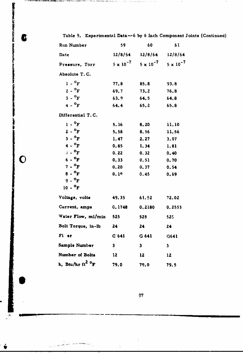
Table 9. Experimental Data-6 by 6 Inch Component Joints (Continued)

Run Number 59 60 61

Date 12/8/64 12/8/64 12/8/64

Pressure, Torr 5 x 10 - 7 5 x 10 - 7 5 x 10- 7

Absolute T. C.

1 - OF 77.8 85.8 93.8

z - °F 69.7 73.2 76.83 - OF 63.9 64.5 64.8

4 - 0F 64.4 65.2 65.8

Differential T. C.

1 - OF 5.36 8.20 11.10

2 - .F 58 8.56 11.563 - OF 1.47 2.27 3.07

4 - 0F 0.85 1.34 1.81

3- 0F 0.22 0,32 0.40

6- F 0.33 0.51 0.70

7 - 0 F 0.20 0.37 0.54

8 - OF 0.10 0145 0.699 0 OF

10 - F

Voltage, volts 49.35 61.52 12. 02

Current, amps 0.1748 0.2180 0.2553

Water Flow, ml/min 525 525 525

Bolt Torque, in-lb 24 24 24

Fi or C 641 G 641 G641

Sample Number 3 3 3

Number of Bolts 12 12 12

h, Btu/hr ft 2 0F 79.0 79.0 79.5

O97

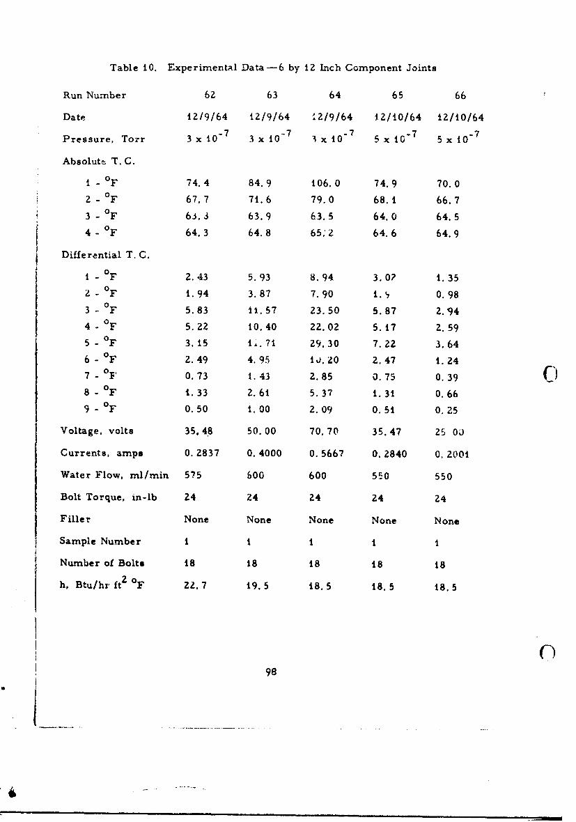
Table 10. Experimental Data-6 by 12 Inch Component Joints

Run Number 62 63 64 65 66

Date 12/9/64 12/9/64 12/9/64 12110/64 12/10/64

Pressure, Torr 3 x 10 7 3 x 10-7 3 x 10- 7 5 x 10 7 5 x 10 7

Absolute T.C.

1 - 0 74.4 84.9 106.0 74.9 70.0

2 - F 67.7 71.6 79.0 68.1 66.7

3 - F 63.3 63.9 63.5 64.0 64.5

4 - 0 F 64.3 64.8 65; ' 64.6 64.9

Differential T. C.

1 - 0F 2.43 5.93 8.94 3.0? 1.35

2 - 0 F 1.94 3.87 7.90 1. , 0.98

3 - 0 F 5.83 11.57 23.50 5.87 2.944 - 0F 5.22 10.40 22.02 5.17 2.59

5 - OF 3.15 1,. 71 29.30 7.22 3.64

6 - °F 2.49 4.95 10.20 2.47 1.247° 0F 0.7 1, 43 2.85 0.7 0. 398 - 0F 1.33 2.61 5.37 1.31 0.66

9 - 0F 0.50 1. 00 2.09 0.51 0.25

Voltage, volts 35. 48 50.00 70.70 35.47 25 0

Currents, amps 0.2837 0.4000 0.5667 0.2840 0.2001

Water Flow, ml/min 575 600 600 550 550

Bolt Torque, in-lb 24 24 24 24 24

Filler None None None None None

Sample Number I i i I i

Number of Bolts 18 18 18 18 18

h, Btu/hr ft 2 oF 22.7 19.5 18.5 18.5 18.5

9898

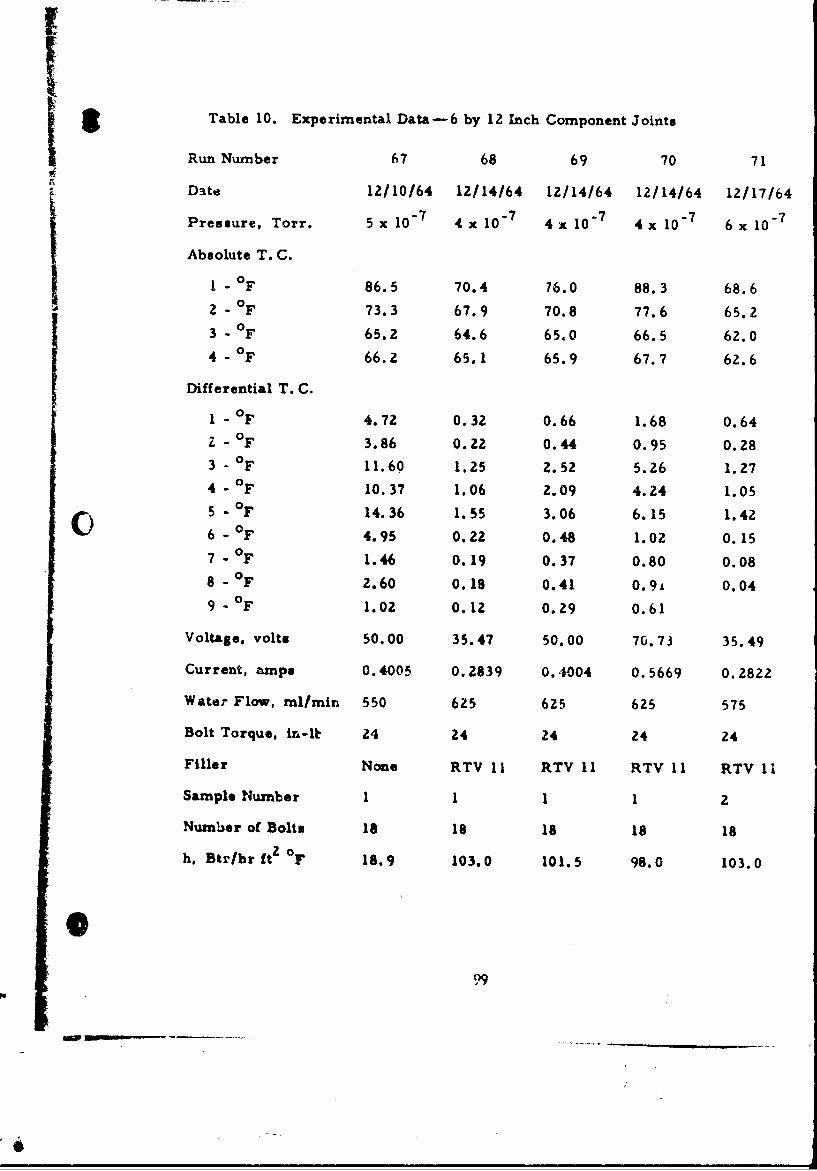
£Table 10. Experimental Data-6 by 12 Inch Component Joints

Run Number 67 68 69 70 71

Date 12/10/64 12/14/64 12/14/64 12/14/64 12/17/64

Pressure, Torr. 5 x 10- 7 4x 10 7 4x 10 7 4x 107 6 x 107

Absolute T. C.

I - OF 86.5 70.4 76.0 88.3 68.6

2 - °F 73.3 67.9 70.8 77.6 65.23 - °F 65.2 64.6 65.0 66.5 62.04 - OF 66.2 65.1 65.9 67.7 62.6

Differential T. C.

I - °F 4.72 0.32 0.66 1.68 0.64. - 0 F 3.86 0.22 0.44 0.95 0.283 - OF 11.60 1,25 2.52 5.26 1.274 - 0 F 10.37 1.06 2.09 4.24 1.05

5 - 0F 14.36 1.55 3.06 6.15 1.42

6 - OF 4.95 0.22 0.48 1.02 0.157 - 0F 1.46 0.19 0.37 0.80 0.088 - 0F 2.60 0.18 0.41 0.9' 0.04

9 - 0F 1.02 0.1Z 0.29 0.61

Voltage, volts 50.00 35.47 50.00 70.73 35.49

Current, amps 0.4005 0.2839 0.4004 0.5669 0.2822

Water Flow, ml/min 550 625 625 625 575

Bolt Torque, ln-lb 24 24 24 24 24

Filler None RTV 11 RTV 11 RTV 11 RTV 11

Sample Number 1 1 1 1 2

Number of Bolts 18 18 18 18 18

h. Btr/hr ft oF 18.9 103.0 101.5 98.0 103.0

99

p.

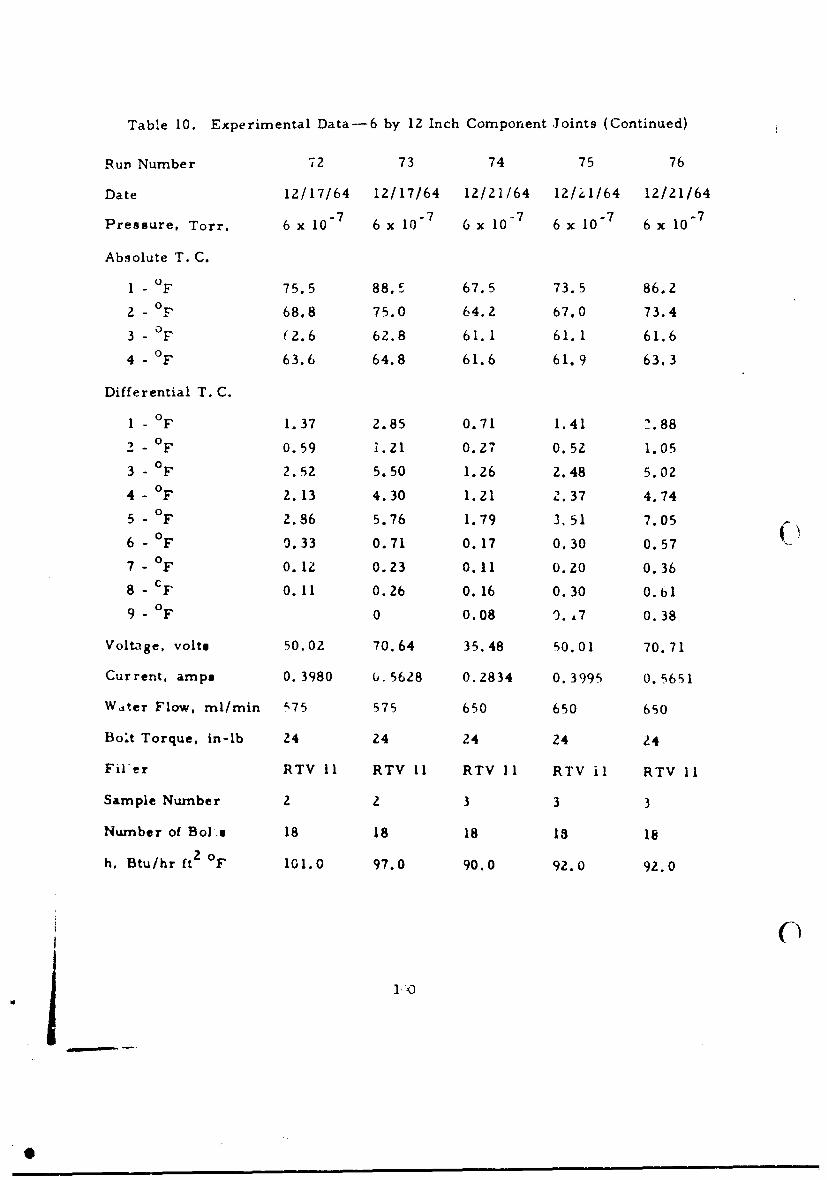
Table 10. Experimental Data-6 by 12 Inch Component Joints (Continued)

Run Number 72 73 74 75 76

Date 12/17/64 12/17/64 12/21/64 12/Zi/64 12/21/64

Pressure, Torr. 6 x 10 -7 7 x6 X 10-7 6 x 10 7 6 x 10- 7

Absolute T. C.

I - 0F 75.5 88.5 67.5 73.5 86.2

2 - 0F 68.8 75.0 64.2 67.0 73.4

3 - 0F (2.6 62.8 61.1 61.1 61.6

4 - 0F 63.6 64.8 61.6 61.9 63.3

Differential T. C.

1 - 0F 1.37 2.85 0.71 1.41 7.88

2- 0F 0.59 1.21 0.27 0.52 1.05

3 - OF 2.52 5.50 1.26 2.48 5.02

4 - F 2.13 4.30 1.21 2.37 4.74

5- 0F 2.86 5.76 1.79 3.51 7.05

6- OF 0.33 0.71 0.17 0.30 0.57

7 - F 0.12 0.23 0.11 0.20 0.36

8 cF 0.11 0.26 0.16 0.30 0.1

9 - F 0 0.08 0.,7 0.38

Voltage, volts 50.02 70.64 35.48 50.01 70.71

Current, amps 0.3980 6.5628 0.2834 0.3995 0.5651

Wdter Flow, mi/min 575 575 650 650 650

Bo't Torque, in-lb 24 24 24 24 24

Filer RTV 11 RTV 11 RTV II RTV iI RTV 11

Sample Number 2 2 3 3 3

Number of Bola 18 18 18 18 18

foF

d1 m

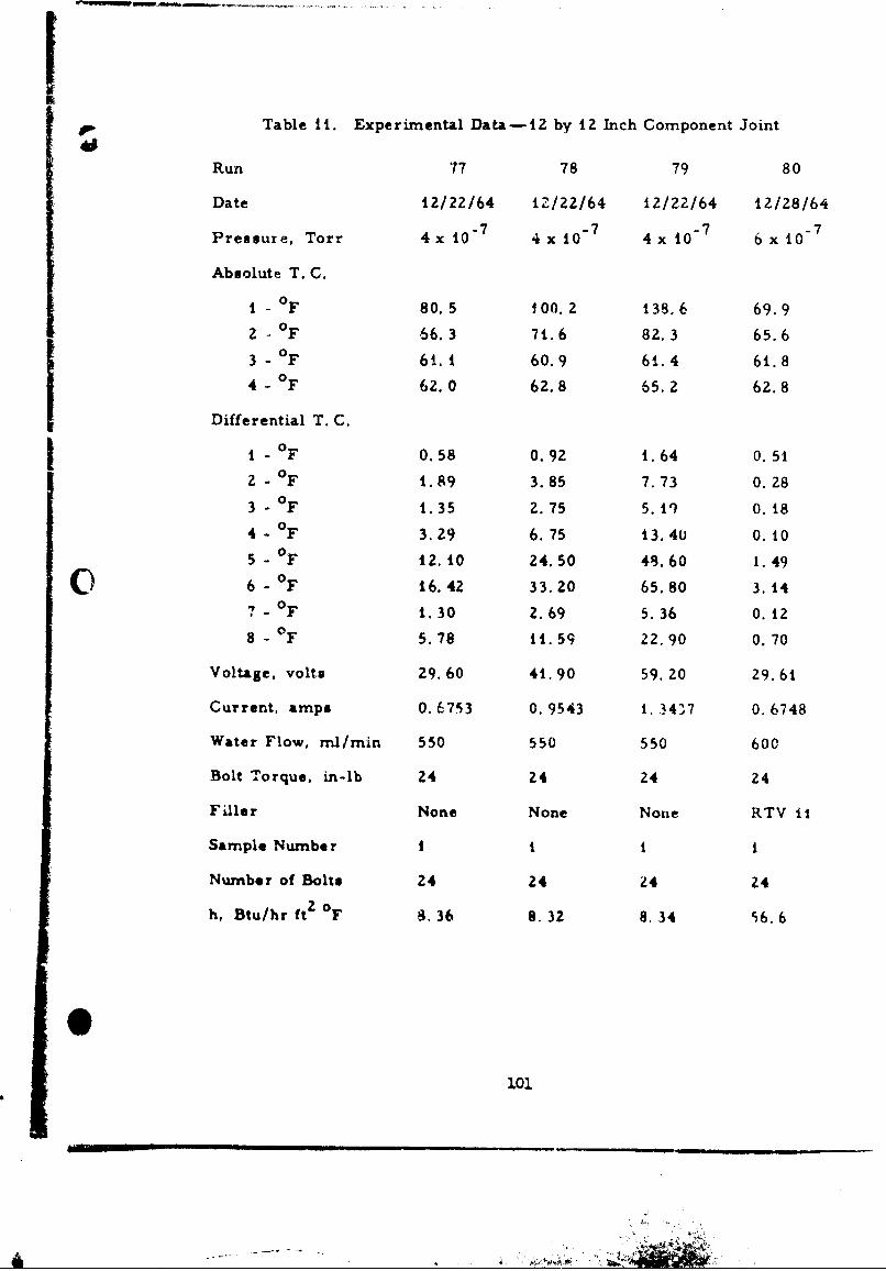
elTable 11. Experimental Data-12 by 12 Inch Component Joint

Run 77 78 79 80

Date 12/22/64 1Z/22/64 12/22/64 12/28/64

Pressure, Torr 4x 10 7 4x 10 7 4x 10 7 6 x 10 - 7

Absolute T. C.

1 - 0 F 80.5 100. 2 138.6 69.9

2 - 0F 66.3 71.6 82.3 65.63 - 0F 61. 1 60.9 61.4 61.8

4 - 0F 62.0 62.8 65.2 62.8

Differential T. C.

I - 0 F 0.58 0.92 1.64 0. 51

2 0 F 1.89 3.85 7.73 0.28

3 - 0 F 1.35 2.75 5.19 0.184 - 0 F 3,29 6.75 13.40 0. 10

5 - 0F 12.10 24.50 48.60 1.49

6 - 0 F 16.42 33.20 65.80 3.14

7 .F .30 2.69 5.36 0. 128 - OF 5.78 11.59 22.90 0.70

Voltage, volts 29.60 41.90 59.20 29.61

Current, amps 0.6753 0.9543 1. 3437 0. 6748

Water Flow, ml/min 550 550 550 600

Bolt Torque, in-lb 24 24 24 24

Filler None None None RTV it

Sample Number I I I I

Number of Bolts 24 24 24 24

h, Btu/hr ft2 oF 8. 36 8.32 8, 34 56.6

101

- -Sl I l l

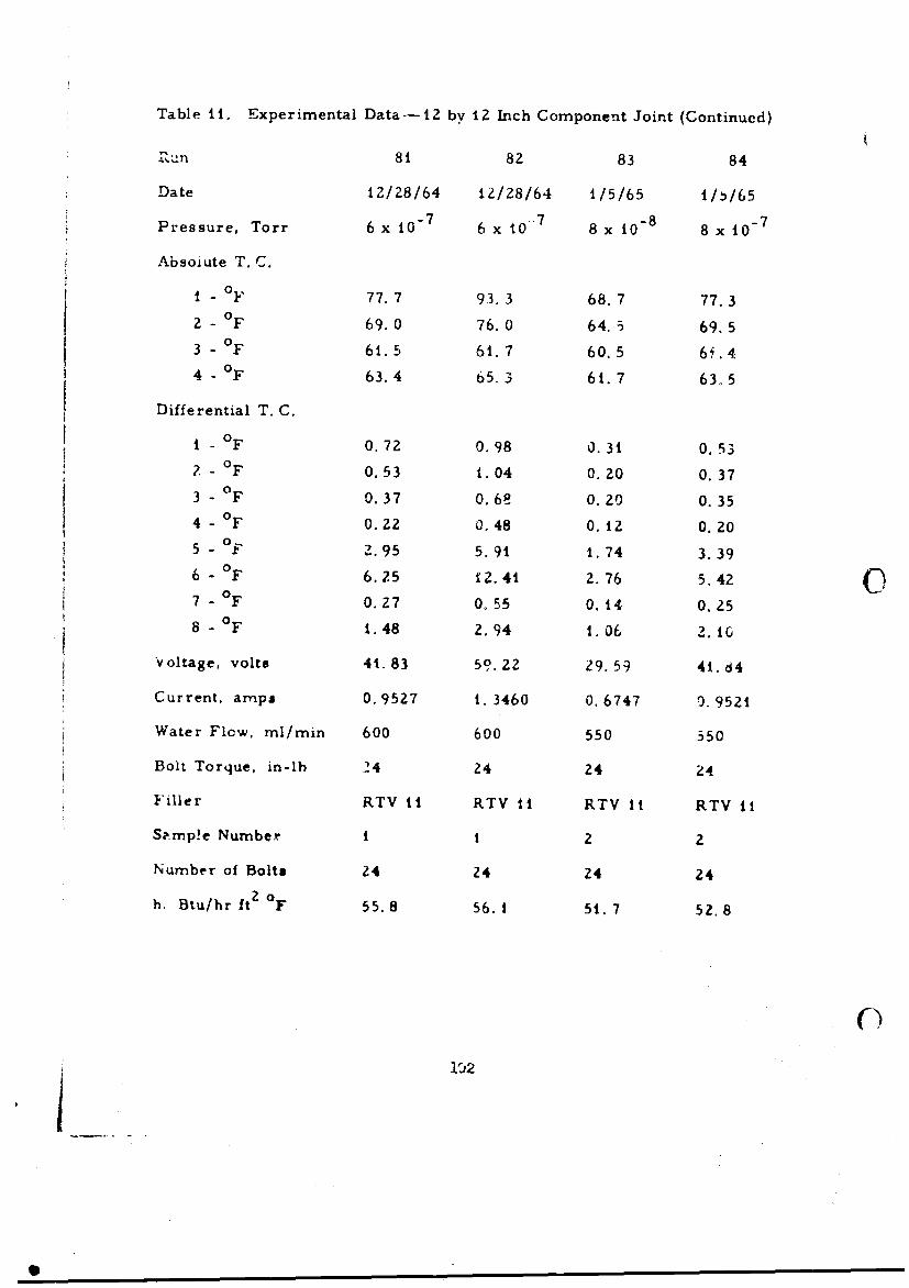
Table 11. Experimental Data--12 by 12 Inch Component Joint (Continued)

lun 81 82 83 84

Date 12/28/64 12/28/64 1/5/65 1/!/65

Pressure, Torr 6 x 10 6 x 0 8 x 8 8 x 10 - 7

Absoiute T. C.

1 - OF 77.7 93.3 68.7 77.3

2 - °F 69.0 76.0 64.5 69.53 - 0 F 61.5 61. 7 60.5 6i.44 - OF 63.4 65.3 61.7 63,5

Differential T. C.

1- OF 0.72 0.98 0.31 0. 53-F 0.53 1.04 0.20 0.37

3 0 F 0.37 0.68 0.20 0.354- OF 0.22 0.48 0. 12 0.205- 0 F 2.95 5.91 t. 74 3.39

6- OF 6.25 12.41 2. 76 5.42 O

7- 0 F 0.27 0°55 0. 14 0.258- OF 1.48 2.94 1. 06 2. 10

)voltage, volts 4t. 83 59.22 29. 59 41.64

Current, amps 0. 9527 1. 3460 0.6747 0.9521

Water Flow, ml/min 600 600 550 550

Bolt Torque, in-lh 24 24 24 24

Filler RTV it RTV 11 RTV It RTV It

Smp!e Number t t 2 2

Number of Bolts 24 24 24 24

h. Btu/hr fto °F 55.8 56. A 51. 7 52, 8

1C'2

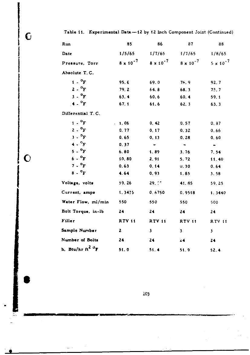
iTable i. Experimental Data-12 by 12 Inch Component Joint (Continued)

Run 85 86 87 88

Date 1/5/65 1/7/65 1/7/65 1/8/65

Pressure, Torr 8x 10 - 7 8 x 10 - 7 8x 10 7 5 x t0 7

Absolute T.C.

I - °F 95.6 69.0 76.9 92.7

2 - 0F 79.2 64.8 68.3 75.7

3 - 0F 63.4 60.6 60.4 59.1

4 - °F 67.1 61.6 62.3 63.3

Differential T. C.

1 - aF 1.06 0.42 0.57 0.87

2 - °F 0.77 0. 17 0.32 0.66

3 - 0F 0.65 0. 13 0.28 0.60

4 - nr 0.37 - - -

5 - 0F 6,80 t.89 3.76 7.54

6 6- F 10.80 2.91 5.72 11.40

7 - 0F 0.63 0.14 U.30 0.64

8 - 0 F 4.64 0.93 1.85 3.58

Voltage, volts 59.26 29. '- 41.85 59.25

Current, amps 1.34!6 0.6750 0.9518 1.3440

Water Flow, ml/mn 550 550 550 500

Bolt Torque, in-lb 24 24 24 24

Filler RTV II RTV II RTV I1 RTV I I

Sample Nunber 2 3 3 3

Number of Bolts 24 24 i4 24

h. Btu/hr ft F 51.0 51.4 51.9 52.4

103

APPENDIX II

STRUCTURAL JOINT TESTS

104

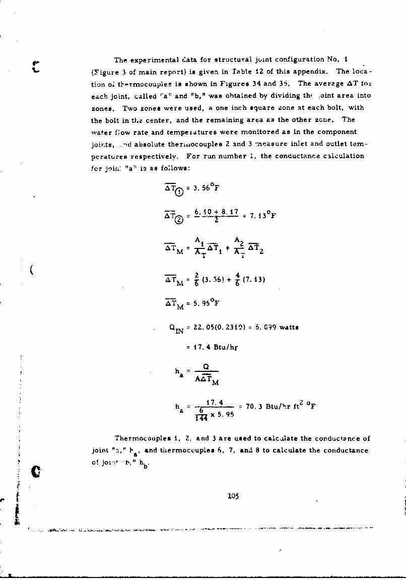
The experimental data for structural joint configuration No. i

(Figure 3 of main report) is given in Table 12 of this appendix. The loca-

tion o, tl'7-rmocouplee is shown in Figures 34 and 35. The average AT iox

each joint, called "a': and "b," was obtained by dividing th( ;oint area into

zones. Two zones were used, a one inch square zone at each bolt, with

the bolt in the center, and the remaining area as the other zone. The

water f;ow rate and temperatures were monitored as in the component

joii.ts, - d absolute therijocouples 2 and 3 neasure inlet and outlet tem-

peratures respectively. For run number A, the conductance calculation

fer joir' "a" is as foilows:

AT = 3. 56°F

= 6.10+8.17 7. 13 0 F

A A2

AT M = 5.T95 0°F

QIN = 22. 05(0. 2310) = 5. C99 watts

= 17.4 Btu/hr

Q

h

17.42o

ha 7. = 70.3 Btu/"r ft Ft-x 5. 95

Thermocouples 1, 2, and 3 are used to calculate the conductance of

joint "a," h , and tiiermockuples 6, 7, and 8 to calculate the conductancea

of jom-)t -t," hbC b'

105:1

Table 13 lists the expe-r, enlal data for structural joint cunfigura-

tion 2. 'The thermocouple locations are shown in Figures 34 and 35. Thib

coniiguration u.iLzes nut plates on one joint, called joint "b" in Table 13.

The results for coniguration 3 are shown in Table 14, and the

thermocouple locations in .Figures 36 and 37. Differential thermocouplc

are located at the same (x, y) coordinates on the back of the angle brackets

and pan ls at the locations shown on Figures 34, 35, 36, and 37.

106

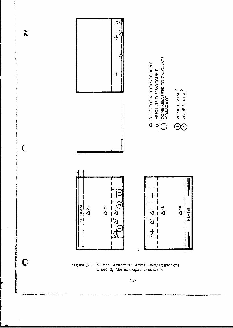
Li)i

WYW

a- 0

Uo0

Li)

zz

ae Lu LUJ LUt0z2: z zCO 0 0 0O<N N

Z- 1-CLU

jCFigure 34. 6Inch Structural Joint, Configurations1 and 2, Thermocouple Locations

107/

--

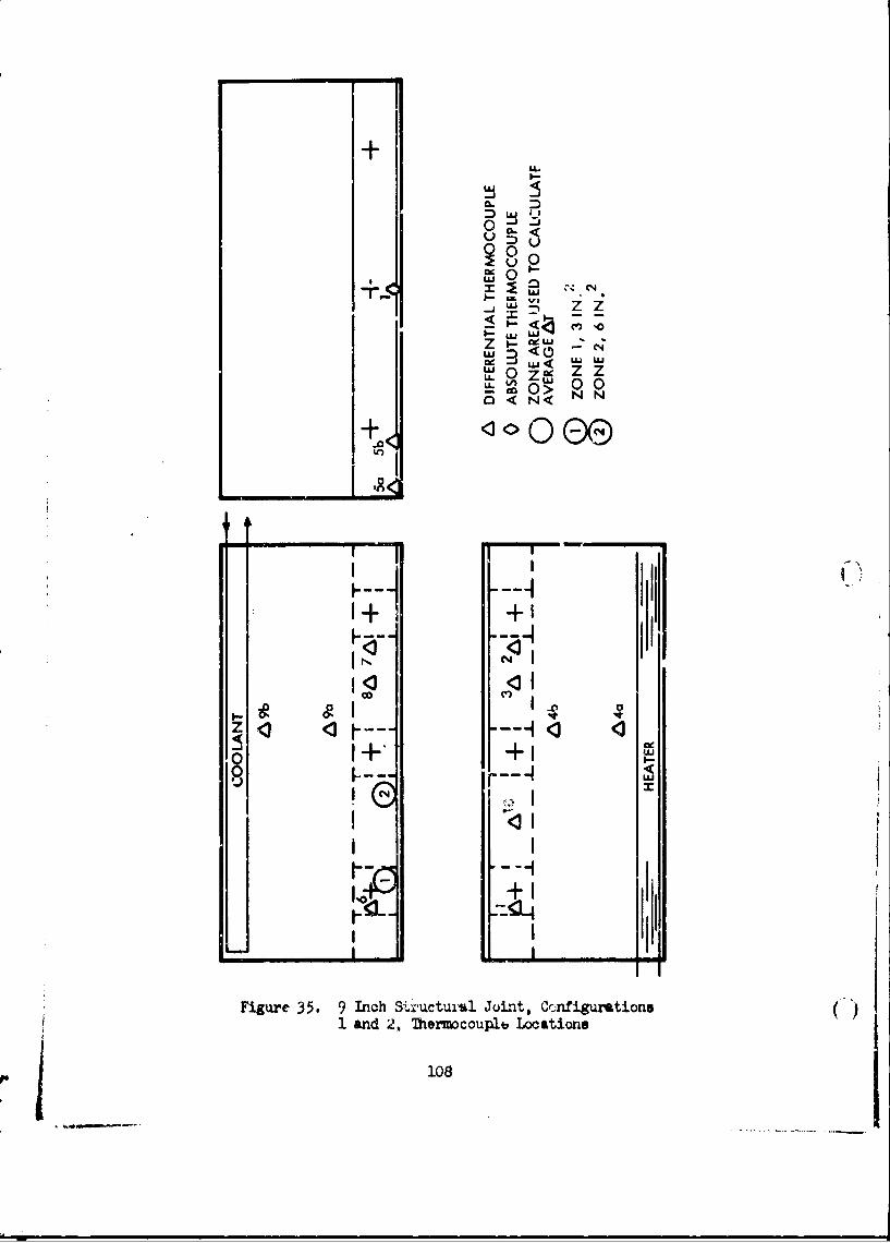
CL

0 0

UU

k~~L1 0-II'

cc 3 (3 U

NN

+ 0

Oj 088I O I

Figure 35. 9 Inch Str'uctui'uJo int, Ccinfiguratione1 and 2, Thermocoupltb Locations

108

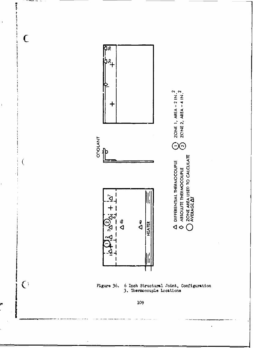
i

Al ____

CCN

z z

- CLaLU

00

LU

wU

r.LI z <

L L LAOZ I.- IW N

C4~33

3. ~ ~ U &Ar~cul Loaton

C4109

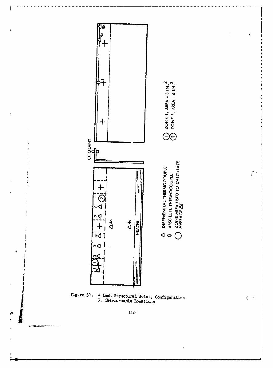
II II

-f.. zz

00N N

0

~UJ

t0z+VZJJ

Z Ii

Figre3'( 9Inchb Structural. Joint, Coafiguration

T o e aIno

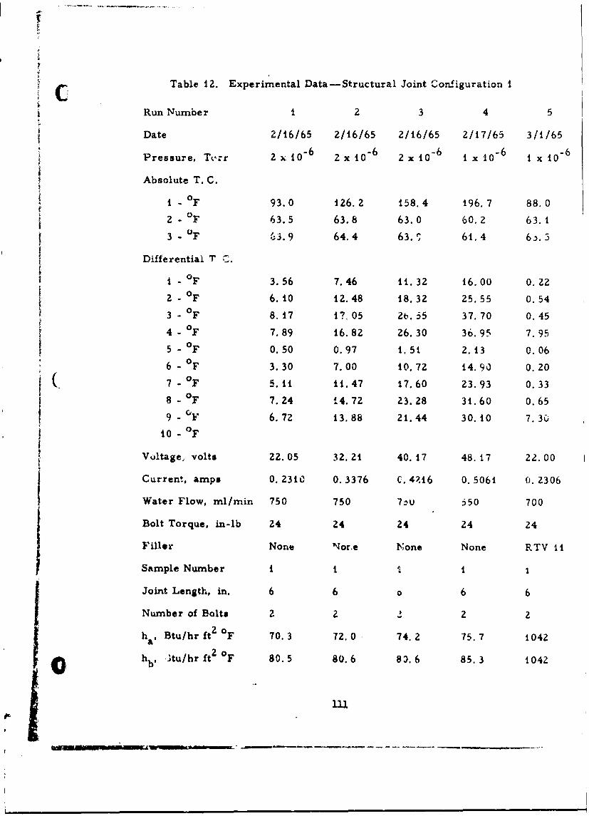
Table i2. Experimental Data-Structural Joint Configuration 1

Run Number 1 2 3 4 5

Date 2/16/65 2/16/65 2/16/65 2/17/65 3//65

Pressure, TL':r 2 x lo-6 6 i x lo- 6 1 x lo-6

Absolute T. C.

i - 0F 93.0 126.2 158.4 196. 7 88.0

2 - 0F 63.5 63.8 63.0 60.2 63.1

.- ,J.9 64.4 63. 61.4 6 .)5

Differential T C.

I - OF 3.56 7.46 11. 32 16.00 0.22

2 - F 6.10 12.48 18.32 25.55 0.54S3 - °F 8. 17 17c 05 2t,. 35 37. 70 0. 45

4 - OF 7.89 16.82 26.30 36.95 7. 95

5 - 0.50 0.97 1. 51 2. 13 0. 06

6 - 0 F 3.30 7.00 10.72 14.90 0.20

7 -0F S. 11 11.47 17.60 23.93 0.33

8 - 0F 7.24 14. 72 23.28 31.60 0.65

9 - "F 6.72 13.88 21.44 30.10 7.3Glo - aOF

Voltage, volts 22.05 32. 21 40. 17 48. t7 22.00

Current, amps 0. 2310 0. 3376 C. 4'.16 0. 5061 0. 2306

Water Flow, ml/min 750 750 7hU 550 700

Bolt Torque, in-lb 24 24 24 24 24

Filler None Nore None None RTV 11

Sample Number I 1 1 t 1

Joint Length, in. 6 6 o 6 6

Number of Bolts 2 2 .- 2 2

ha , Btu/hr ft 2 oF 70.3 72.0 74.2 75. 7 1042

hb , 'tu/hr ft 2 oF 80.5 80.6 80.6 85.3 1042

11

I i ml, • • • •~- - - - -. • •• __s _

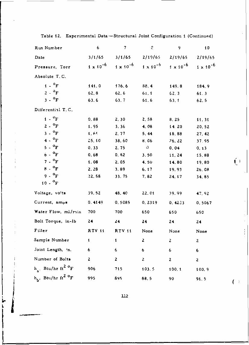
Table 12. Experimental Data-Structural Joint Configuration i (Continued)

Run Number 6 7 2 9 10

Date 3/1/65 3/1/65 2/19/65 2/19/65 2/19/65

Pressure, Torr 1 x 10 6 i x to- 6 1 x io- 6 x 10 6 1 x i0-6

Absolute T. C.

1 - F 41.0 176.6 88.4 149.8 184.9

2 - 0F 62.8 62.6 6i.1 62.3 61.3

3 0 F 63.6 63.7 61.6 63.1 62.5

Dilferential T. C.

1 - OF 0.88 2.30 2.58 8.25 11.31

2 - 0F 1.95 3.36 4.08 14 20 20.52

3 - °F 1 2.77 5.44 18.88 27.42

4 - OF Z5.10 38.60 8. 06 ?6.22 37.95

5 - °F 0.33 2.75 0 0.04 0.13

6 - °F 0.68 0.82 3.50 141.24 15.88

7 - .F 1.08 2.05 4.50 14.80 19.80

8 - OF 2.28 3.89 6. 17 19.93 26.08

9 - 0F ,2.58 33. 75 7.82 24.17 34.85

10 - 0F

Voltage, volts 39.52 48.40 22.01 39.99 47. q2

Current, amps 0.4149 0.5085 0.2319 0.4223 0.5067

Water Flow, ml/mrin 700 700 650 650 650

Bolt Torque, in-lb 24 Z4 24 24 24

Filler RTV 11 RTV 11 None None None

Sample Nlirnber I 1 2 2 2

Joint Length, ;n. 6 6 6 6 6

Number of Bolts 2 2 2 2 2

h Btu/hr ft 2 oF 906 715 103.5 100. 1 100.9a

hb, Btw/hr it oF 995 895 88.5 90 96.5

,m ,o , , ' 112

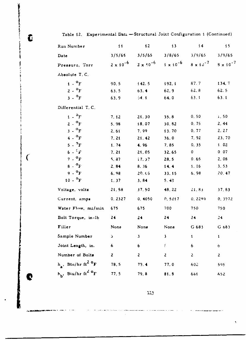
c Table 12. Experimental Dat. -Structural Joint Configuration I (Continued)

Run Nunber 11 12 13 14 15

Date 3/5/65 3/5/65 3/8/65 3/9/65 3/9/65

Pressure, Torr 2 x 10 - 6 2 x 0 6 1 x 10 - 6 8 x 1j 7 8 X 10 - 7

F

Absolute T. C.

1 - OF 90.5 142. 5 192.1 87.7 134.702 - F 63.5 63.4 6Z.9 62.8 62.5

3 - 0F 63.9 '4. 1 64.0 63.1 63A1

Differential T. C,

I - F 7.12 21.30 35.8 0.50 1.500

2- F 5.98 18.07 30.82 0. 75 2.440

3 - F 2.61 7.99 13.70 0. 77 2.27

4 - 0 F 7. 21 21.42 36.0 7. 92 23.70

5 - OF i. 74 4.96 7.85 0. 35 1 02

6 -Fi 7.21 21.05 32.65 0 o07

7 -OF . 87 i7.i7 28.5 0.65 2. 08

8 - 0 F 2. 84 8. 36 14.4 1, 16 3.53

9 - °F 6.98 20. 5 33. 15 6.98 20.47

10 - 0 F I. 37 3.84 5.40

Voltage, volts 21.58 37.50 48.22 2i.8 37.83

Current, amps 0, 2327 0. 4050 0. 5.117 0. 2299 0. 3972IWater Flow, mi/min 675 675 700 750 750

Bolt Torque, in-lb 24 Z4 24 24 24

Filler None None None G 683 G 683

Sample Number 1 3 3 1 1

Joint Length, in. 6 6 6 6

Number of Bolts z ' 2 2

h Btu/hr ft 2 0 F 78.5 79.4 77.0 602 595

Shb@ Btu/hr ft 4 F 77.5 79.8 81. S 68t 652

1-3

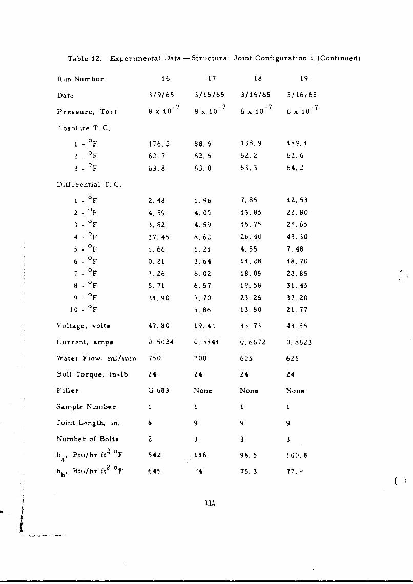
Table 1Z. Experimental Data -Structural Joint Configuration i (Continued)

Run Number 16 17 18 19

Date 3/9/65 3/15/65 3/16/65 3/16/65

Pressure, Torr 8 x 10- 7 8 x 10 -7 6 x 10 -7 6 x i0- 7

.',bsolute T. C.

1 - °F 176.5 88.5 138.9 189.1

2 - 0F 62.7 62. 5 62. 2 62.6

3 - eF 63.8 63.0 63.3 64.2

Diffe-rential T. C.

1 - 0 F 2. 48 1.96 7.85 12.53

2 - 0 F 4.59 4.05 13.85 22.80

3 - 0 F 3.82 4. 59 15.7S 25.65

4 - 0 F 37.45 8. 6Z 26. 40 43.30

5 - °F 1.66 1. 21 4.55 7,48

6 - °F 0. 21 3.64 11.28 18.70

7-- °F 3. 26 6,02 18.05 28.85

8 - 0 F 5. 71 6. 57 19.58 3t.45

9.. 0 F 31.90 7. 70 23, 25 37.20

i0 - 0 F . 86 13.80 21.77

Voltage, volts 47.80 t9. 4A 33. 73 43. 55

Current, amps 0 5024 0. 3841 0.6672 0. 8623

Water Flow. mI/min 750 700 65 625

Bolt Torque, in-lb 24 24 24 24

Filler G 683 None None None

Sample Number I I t 1

Joint Length, in. 6 9 9 9

Number of Bolts 2 3 3 3h , Btu/hr ft F 54 t16 98.5 00.

hb, _%tu/hr ItZ oF 645 '4 75. 3 77.A(

t

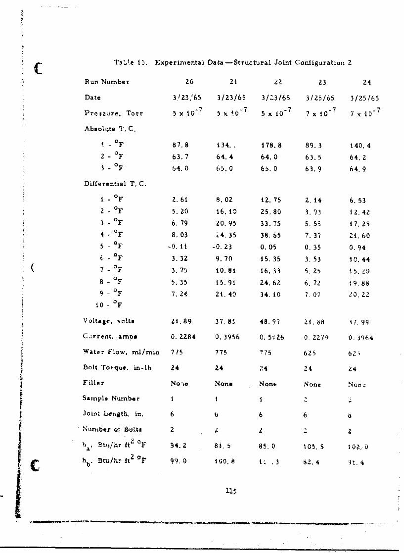
Ta',.e 13. Experimental Data-Structural Joint Configuration 2

Run Number Z0 21 2 23 24

Date 3!23,'65 3/23/65 3/23/65 3/25/65 3/25/65

Pre.joure, Torr x1 7 xO 7 7i 7 75 x 10 5 X 0 5 x 10 - 7 x 10 - 7 x 1 0-

Absolate T, C.

I F 87.8 134.. 178.8 89.3 140.42- °F 63.7 64.4 64.0 63.5 64.2

3- °F 64.0 65.0 6t. 0 63.9 64.9

Differential T.C.

1 F 2.61 8.02 12.75 2,14 6.53

2 - "F 5.20 16.10 25.80 3.93 12,423 0 F 6.79 20.95 33.75 5. 55 17.25

4- °F 8.03 24.35 38.65 7.37 21,605 - F -0. 1I -0.23 0.05 0.35 0.94

- OF 3.32 9.70 15.35 3.53 10.44( 7 - OF 3.75 10.81 16.33 5.25 15.20

8 - F 5. 35 15.91 24.62 6.72 19.88

9 -"°F 7. 24 21.40 34.10 7.Z07 0.22

10 - OF

Voltage, volts 21.89 37.85 48.97 21.88 37.99

Cirrent, ampS 0. 2284 0.3956 0.5126 0. 2279 0.3964

Water Flow. ml/min 715 775 775 625

fBolt Torque. in-lb Z4 24 24 24 24

Filler No-ie None None None NonZ

Sample Number I 1 1 2 _

Joint Length, in. 6 6 6

Number oliSit* 2 2 2 2 2

h, Bt "hr 3 F 34.2 81, $ 85.0 05, .- 0. .0

h -. Btti/hr ft z . 9 "9 0 100 8,b-Q4 , .' t

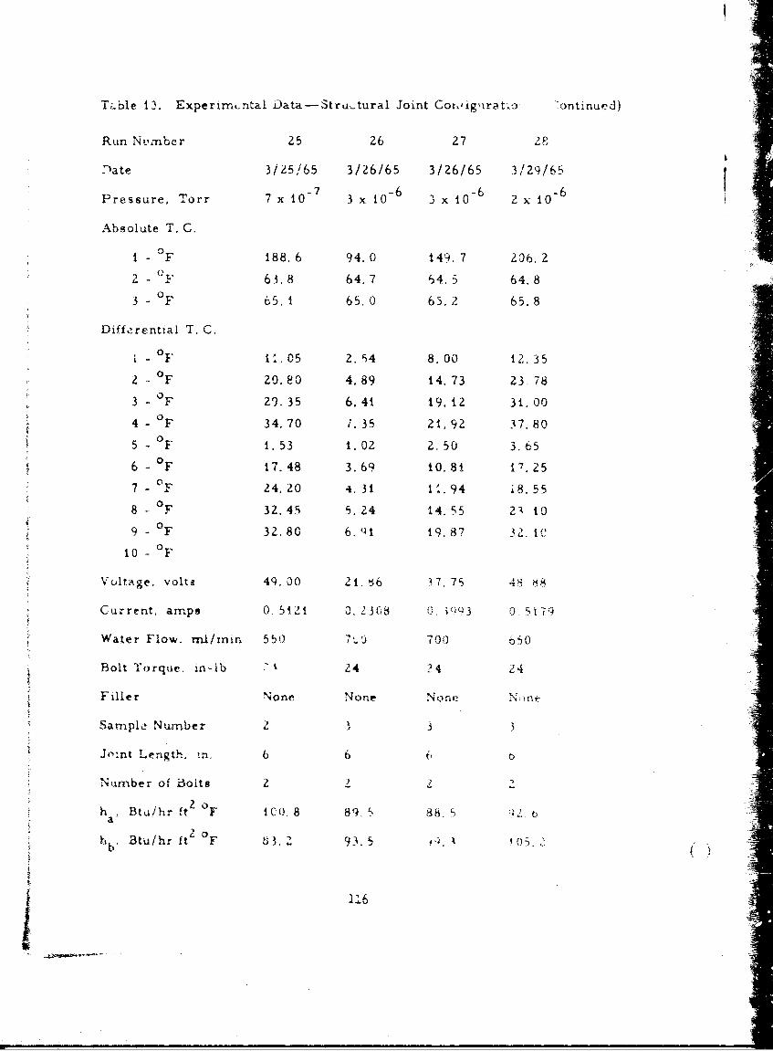
TLble 13. Experirnntal Data-Stru.tural Joint Coxigurat.o :ontinued)

Run Nvrnber 25 26 27 -,8.

Date 3/251/65 3/26/65 3/26/65 3/29/65

Pressure, Torr 7 x 10 - 3x0 3x 10 6 2 x 106

Absolute T. C,

1 - F 188. 6 94. 0 149. 7 206. 2

2- t 63. 8 64. 7 64. 5 64.83 F 65. 1 65,0 65.2 65. 8

Differential T, C.

L - F il. 05 2. S4 8. 00 12. 35

2 - 0 F 20.80 4.89 14. 73 23 78

3 - OF 29. 35 6.41 19. 12 3t. 00

4 - °F 34. 70 i. 35 21,92 37.80

5 - oF 1, 53 1. 02 2, 50 3.65

6 - F 7.48 3.69 t0.81 17. 25

7 - 0 F 24. 20 i. 31 11. 94 I8. 55

8 ,- oF 32.45 5. 24 14. 55 2 t009- F 32.80 6.91 19.87 32.1

t0 - F

Voltage, volte 49.00 21. 66 37, 75 48 ?8-

Current, amps 0. 5121 0. 23G8 0. 1-.3 0 5-?

Water Flow. min/m 550 7*,, 700 050

Bolt Torque. in-ib 24 ? 4 Z4

Filler None None Noc neN )ne

Sample Number 2 3 3 3

Jront Length, n. 6 6 6 .

Number of Bolts 2 2 2 Z

Z 0h Btu/hr ft F I0. 8 89. 8 8.

h Btu/hr ft F 8 3. Z 93.5 ,). 5 '05.

j 326

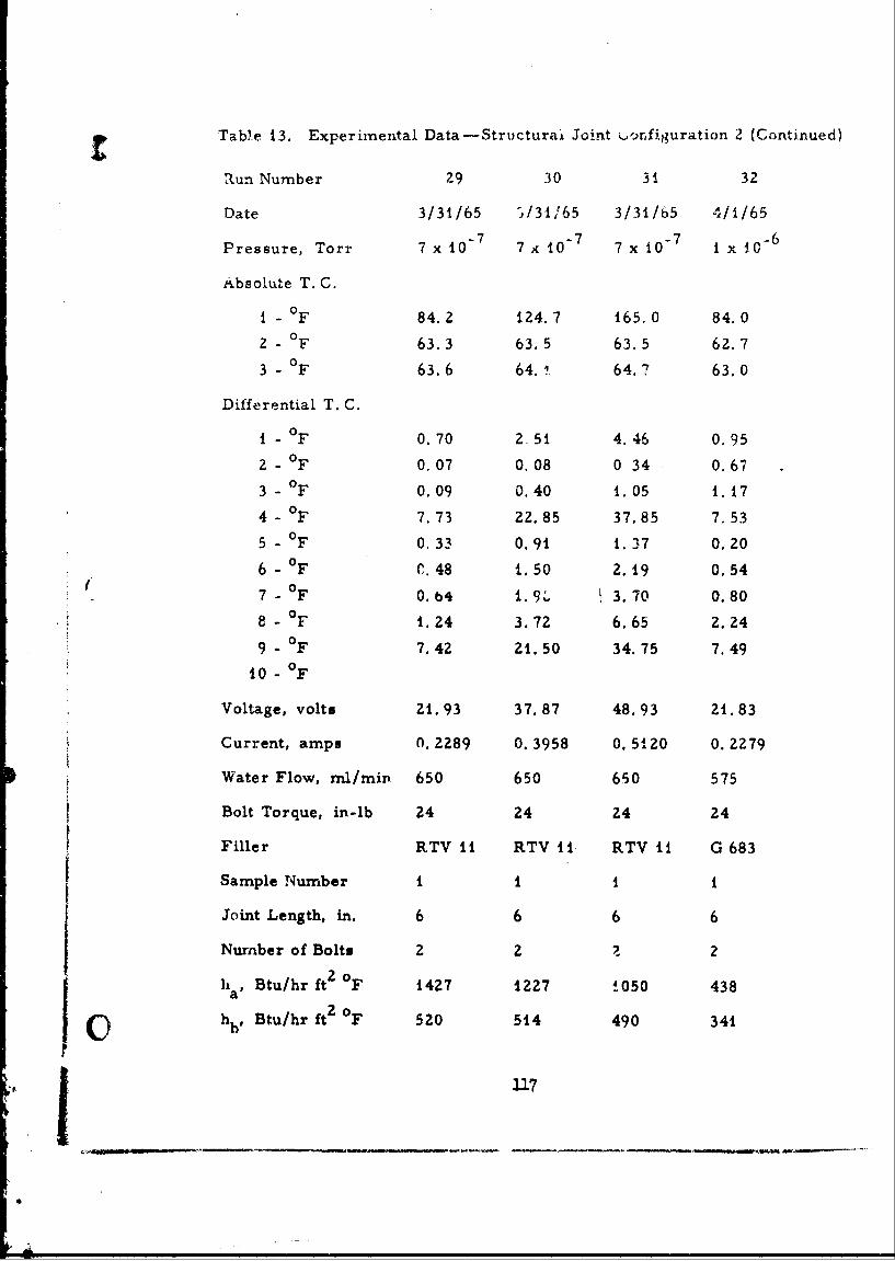
r Table 13. Experimental Data-Structurai Joint uonfiguration 2 (Continued)

Run Number 29 30 31 32

Date 3/31/65 -/31/65 3/31/65 4/1/65

Pressure, Torr 7 x 10 7 7 -107 -x 07 1 x 10 - 6

Absolute T. C.

1 - 0F 84.2 124.7 165.0 84.0

2 - 0F 63.3 63.5 63.5 62.73 - 0F 63.6 64.. 64.7 63.0

Differential T. C.

1 - OF 0.70 2.51 4.46 0.95

2 - OF 0. 07 0.08 0 34 0.673 - OF 0.09 0.40 1. 05 1. 17

4 - OF 7.73 22.85 37.85 7. 53

5 - OF 0. 33 0.91 1.37 0.20

6 - OF C, 48 1.50 2.19 0.54( 7 - F 0.1,4 1.9L 3.70 0.80

8 - OF 1.24 3.72 6.65 2.24

9 - F 7.42 21.50 34.75 7.4910 -OF

Voltage, volts 21. 93 37.87 48.93 21.83

Current, amps n. 2289 0. 3958 0. 5120 0. 2279

Water Flow, mI/min 650 650 650 575

Bolt Torque, in-lb 24 24 24 24

Filler RTV 11 RTV 11 RTV i1 G 683

Sample Number 1 1 1 1

Joint Length, in. 6 6 6 6

Number of Bolt. 2 2 2 2

ha , Btu/hr ft 2 OF 1427 1227 !050 438

h., Btu/hr ft 2 OF 520 514 490 341j 117

-,9..

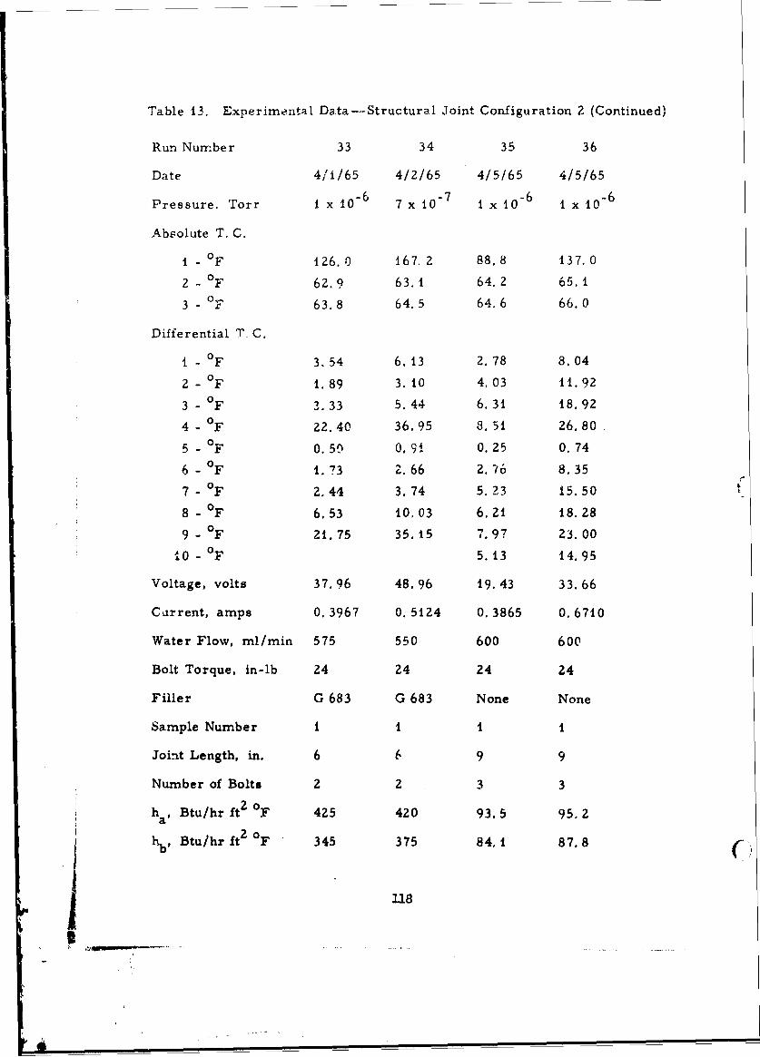
Table 13. Experimental Data--Structural Joint Configuration 2 (Continued)

Run Number 33 34 35 36

Date 4/1/65 4/2/65 4/5/65 4/5/65

Pressure. Torr i x 10 - 6 7 x i0 7 1 x 10 6 1 x 10 6

Absolute T. C.

I - 0F 126.0 167, 2 88.8 137.0

2- 0 F 62.9 63.1 64.2 65.1

3 - OF 63.8 64.5 64.6 66.0

Differential T. C.

I - 0F 3.54 6.13 2.78 8.04

2 - 0F 1.89 3.10 4. 03 11.92

3- 3.33 5.44 6. 31 18.92

4 - 0F 22.40 36.95 8. 51 26.80

5 - 0F 0.50 0.9i 0.25 0.74

6 - °F 1. 73 2. 66 2. 76 8.35

7 - °F 2.44 3.74 5.23 15.50

8 - °F 6.53 10.03 6.21 18.28

9 - 0F 21.75 35.15 7.97 23.00

a0 - OF 5.13 14.95

Voltage, volts 37.96 48.96 19.43 33.66

Current, amps 0.3967 0.5124 0.3865 0.6710

Water Flow, ml/min 575 550 600 600

Bolt Torque, in-lb 24 24 24 24

Filler G 683 G 683 None None

Sample Number 1 1 1 1

Joint Length, in. 6 6 9 9

Number of Bolts 2 2 3 3

ha , Btu/hr ft2 OF 425 420 93.5 95,2

hb, Btu/hr ft2 oF 345 375 84.1 87.8

31

5mlmm

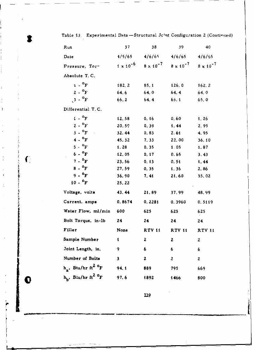
Table 13. Experimental Data-Structural Jc-nt Configuration 2 (Contin ued)

Run 37 38 39 40

Date 4/5/65 4/6/61 4/6/65 4/6/65

Pressure, Tor- I x 10 -6 8 x 10 7 8 x 10 7 8 x 10-7

Absolute T. C.

i - 0 F 182. 2 85.1 126.0 162.2

2 - °F 64.6 64.0 64.4 64.0

3 - 0F 66.2 64.4 65.1 65.0

Differential T. C.

I - F 2.58 0.16 0.60 1.26

2 - °F 20.59 0.39 1.44 2.99

3 - 0 F 32.44 0.83 2.61 4.95

4 - OF 45.32 7.33 22.00 36.10

5 - °F 1.28 0.35 1 05 1.87

6 - 'F 12.05 0.17 0.65 3.43

7 7- F 23.56 0.13 0.51 1.4408 - F 27.59 0.35 1.36 2.86

9 - 0F 36.90 7.41 21.60 35.02

10 - 0F 25.22

Voltage, volts 43.44 21. 89 37.99 48.99

Current, amps 0.8674 0. 2281 0. 3960 0.5119

Water Flow, ml/min 600 625 625 625

Bolt Torque, in-lb 24 24 24 24

Filler None RTV 11 RTV 11 RTV 11

Sample Number 1 2 2 2

Joint Length, in. 9 6 6 6

Number of Bolts 3 2 2 2

ha , Btu/hr ft2 oF 94. 1 889 795 669

Shb , Bu/hr ft2 oF 97.6 1892 1466 800

119

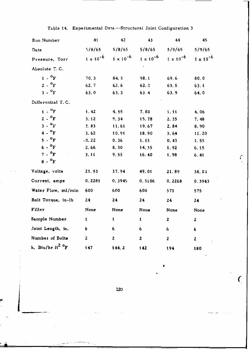
Table 14. Experimental Data-Structural Joint Configuration 3

Run Number 41 42 43 44 45

Date ',/8/65 5/8/65 5/8/65 5/9/65 5/9/65

Pressure, Torr 1 x 10-6 1 x 0 - 6 1 x 0 "-6 x 10- 6 1 x 10-6

Absolute T. C.

I - 0F 70.3 84.5 98.1 69.6 80.0

2 - 0 F 62.7 62.6 62.?Z 63.5 63A1

3 - 0 F 63.0 63.3 63 4 63.9 64.0

Differential T. C.

1 - 0 F 1.42 4.55 7.80 1.11 4.06

2 - OF 3.12 9.34 15.78 2.35 7.483 - 0°F 3,83 11.61 19.67 2.84 8.90

4 - °F 3.62 10.91 18.90 3.64 11.20

5 - OF -0.22 0.36 1.15 0.43 1.55

6 - °F 2.66 8.30 14.35 1.92 6.15

7 - OF 3.11 9.55 16.40 1.98 6.418 - 0OF

Voltage, volts 21.93 37.94 49.01 21.89 38.01

Current, amps 0. 2281 0. 3949 0. 5106 0. 2268 0. 3943

Water Flow, ml/min 600 600 600 575 575

Bolt Torque, in-lb 24 24 24 24 24

Filler None None None None None

Sample Number I 1 1 2 2

Joint Length, in. 6 6 6 6 6

Number of Bolts 2 2 2 2 2

h, Btu/hr ft 2 °F 147 144. 2 142 194 t80

(

120

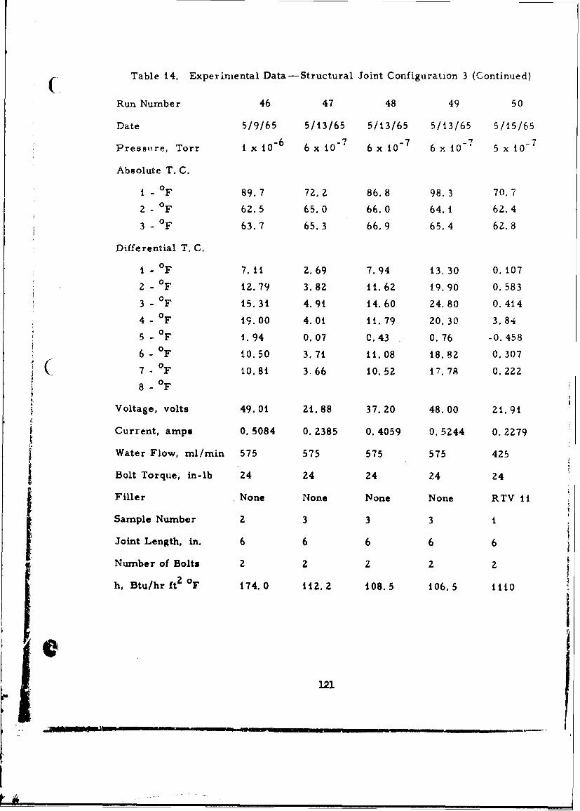
(Table 14. Experimental Data--Structural Joint Configuration 3 (Continued)

Run Number 46 47 48 49 50

Date 5/9/65 5/13/65 5/13/65 5/13/65 5/15/65

Presslre, Torr i x 106 6 x 10 7 6 x 10 7 6 x i0-7 5 x 10

Absolute T. C.

1 - °F 89.7 72.2 86.8 98.3 70.7

2 - OF 62.5 65.0 66.0 64.1 62.4

3 - oF 63.7 65.3 66.9 65.4 6Z. 8

Differential T. C.

i - OF 7. 11 2.69 7.94 13.30 0. 107

2 - OF 12.79 3.82 11.62 19.90 0. 583

3 - OF 15.31 4.91 14.60 24.80 0.414

4 - 0F 19.00 4.01 11. 79 20.30 3.84

5 - 0F 1.94 0.07 0.43 0.76 -0. 45806 - F 10.50 3.71 11.08 18.82 0. 307

7 -0 F 10.81 3. 66 10. 52 17.78 0.222- 0 F8 - OF

Voltage, volts 49.01 21.88 37.20 48.00 21.91

Current, amps 0. 5084 0. 2385 0. 4059 0. 5244 0. 2279

Water Flow, ml/min 575 575 575 575 425

Bolt Torque, in-lb 24 24 24 24 24

Filler None None None None RTV 11

Sample Number 2 3 3 3 1

Joint Length, in. 6 6 6 6 6

Number of Bolts 2 2 z 2 2

h, Btu/hr ft2 °F 174.0 i2.2 108.5 106.5 1110

@,I

• = 2 _. - . . . . . . . .I I. _. I ] . ... I I II I"" ' "

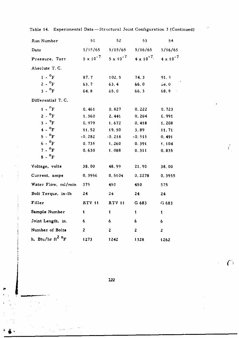
Table 14. Experimental Data -Structural Joint Configuration 3 (Continued)

Run Number 51 52 53 54

Date 5/15/65 5/15/65 5/16/65 5/16/65

Pressure, Torr 5 x 10 7 5 x 10 - 7 4x 10 - 7 . 4x 10 - 7

Absolute T. C.

1 - °F 87.7 102.5 74.3 91.3

2 - °F 63.7 63.4 66.03 - 0F 64.8 65.0 66,3 68.9

Differential T. C.

1 - °F 0.461 0.827 0.222 0.723

2 - 0 F 1.560 2.441 0.284 c. 9913 - 0F 0.979 1.672 0.418 1.208

4 - 0 F 11.52 19.50 3.89 11.715 - 0F -0. 282 -0.218 -0.515 0.491

6 - 0 F 0.735 1.260 0.391 1.104

7 - 0F 0.630 1.088 0.311 0.835

8 -0 F

Voltage, volts 38.00 48.99 21. 90 38.00

Current, amps 0.3956 0.5104 0.2278 0.3955

Water Flow, ml/min 375 450 450 575

Bolt Torque, in-lb 24 24 24 24

Filler RTV 11 RTV 11 G 683 G 683

Sample Number i i i i

Joint Length, in. 6 6 6 6

Number of Bolts 2 2 2 2

2Zoh, Btu/hr ft F 1273 1242 1328 1262

122

' t

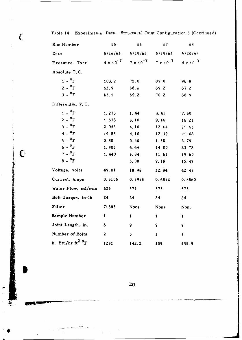
Table 14. ExperimenLal Data-Structural Joint Configuration 3 (Continued)

Run Number 55 56 57 58

Date 5/16/65 5/19/65 5/19/65 5/20/65

Pressure, Torr 4x 10 7 7 x 10 - 7 7 x 10 - 7 4x 10 - 7

Absolute T. C,

i - 0F 103.2 75.0 87.0 96.8

2 - 0F 63.9 68.o 69.2 67.2

3 - 0F 65.1 69.2 70.2 68.9

Differential T. C.

1 - 0F 1.273 1.44 4.41 7.60

2 - 0F 1.678 3. 10 9.46 16.21

3 - 0F 2.043 4. 10 12.64 21.63

4 - F 9.85 4. 10 12.39 21.08

5 - F 0.80 0.40 1.50 2.78

6 - OF 1.905 4.64 14.00 23. 7'8

7- 0F 1.440 3.84 11.61 19.60

8 - 0F 3.00 9.18 15.47

Voltage, volts 49.01 18.98 32.84 42.45

Current, amps 0.5105 0.3958 0.6852 0.8860

Water Flow, ml/min 625 575 575 575

Bolt Torque, in-lb 24 24 24 24

Filler G 683 None None None

Sample Number 1 1 1 i

Joint Length, in. 6 9 9 9

Number of Bolts 2 3 3 3

h, Btu/hr ft 2 0 F 1231 142.2 139 135.5

1.23

APPE\DIX III

SCRIPT F COMFJTMl PROGRAM4 PRINT OUT

124

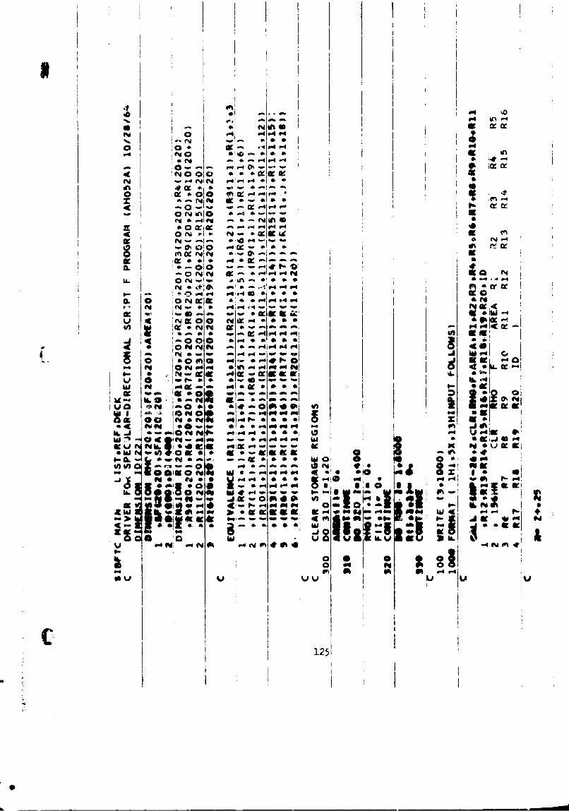
04 0.

N C)11 xwc

1 * 01 40 t, r 4

a.e .41 *-a4 Nin

-- 4NIN JK 0 o-1S 49

- ofI or

IN w -4. f* jOFwj:: a 0 r-4u 39 I N Xg .

]o N fm f 4 r4i cc -£i a' a ~n i &.I W

a W imN coa M a Vol 0 V4.0 L K-40

at00 *4~ ~ S Di ac

Coo 0-~' ;om 0: In' .i

OW -0 c 0 l 0 ft a- m tl w 0IU. Im 0O1*-~4. U

aIE P-4 PO r4 " 1 *: t Lm

ri* OV4 10 4p1

c0- a mma as

v 04 Pm 0.0 4 4 . ev fn in

1-251

'C

II b

VC - o

lk- ii -J ad

4W 0. f

* . 0 I 4 ia In v 01 P4 P n a,

0'- 0% WN Qk9 0 £ -

do V44 x of a- &iX. 46. 4 "P- 0 0- * 4i 1 ~-- -

WOO 11 o). w - I

4wlt - Z' - ' ot I-o * -* * * pg ~ -- p~e g' -~ a -.-Cowgfi.. 4. . .* ~ 4. * S S Q * ~ 4.I0'-~ ~~~~~~~ 4u -'UI- 0 Z -K .( - - I n -:'

3Ea03~-~' - C.4 NbZ~P*uvu .4-*0~g

~~rj

p

*IISV ~wI1 4

CI 1127

I K

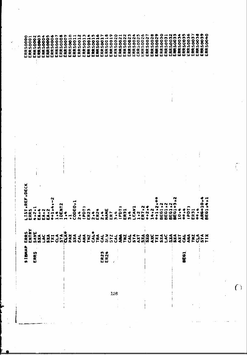
o, r 4. 4 6 0o C -4 N 4d 0I6 0eN 4 Or6 0u- * '?60C0 0000 4~~. 0 0 NNNNNN9coss 88

wwK 1 N t"

P4 NN a M+Nf' 046: -0 4 4' I- - M 4t w 4 )o , N r e .+ $-. 4 P

0) CK N N b & a~ P4 W AP skioko a &cc" &so44$-u444-M 4049 a a &.4I40 04L WNOIK <a a&.F2 W &w+# *wwtD 0* *o' Kwl

ILI

~, a

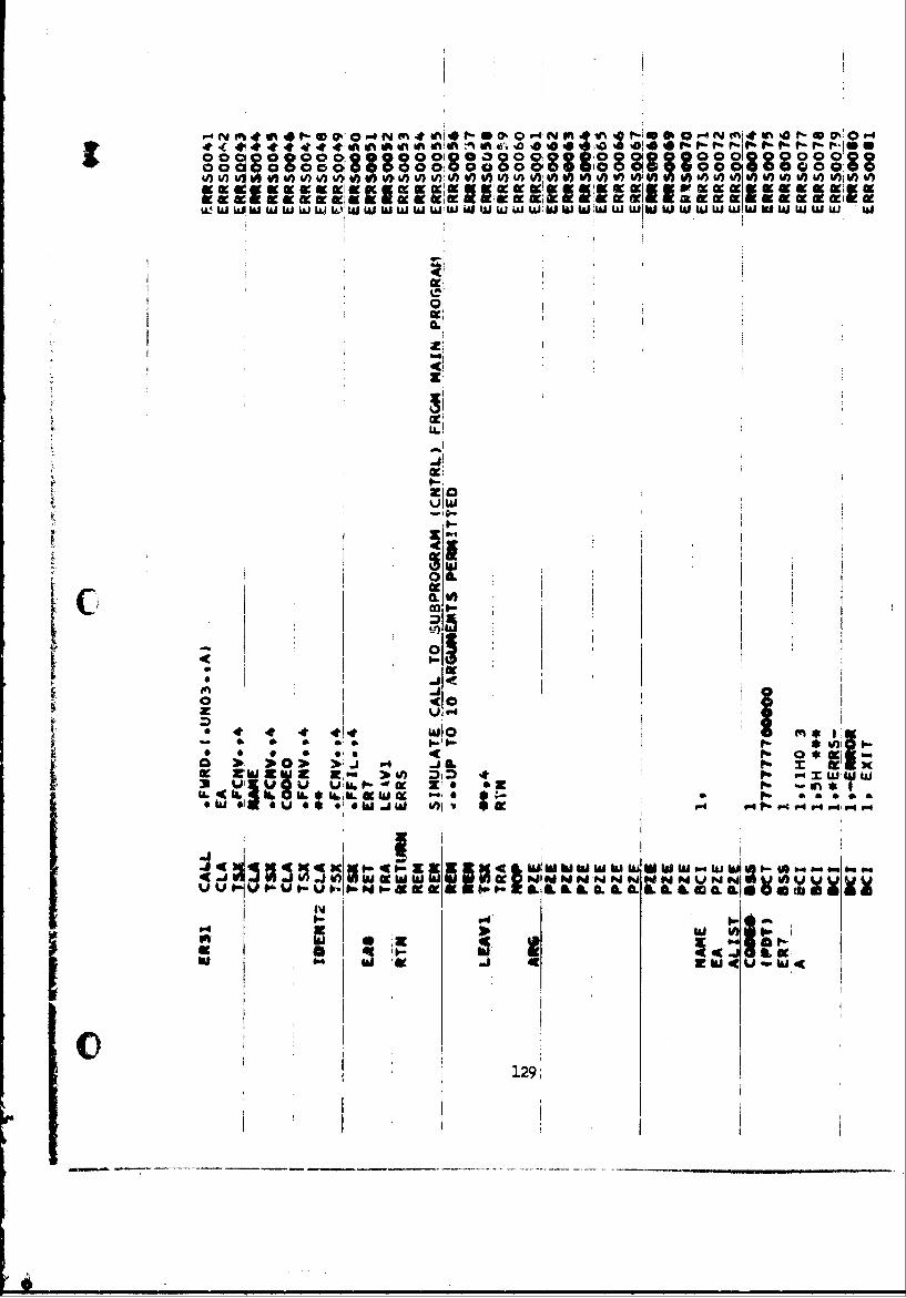
-- C4 e-o in r- ry M- r-" -' t

00 li 0O0 08820 0 09 0V)V)v 1 ) )V)V 00 i A )Uv) ) 6,V )AV) V) - ) V7U U1,V)V o ) U)V)WiV )

0,

0.

ILI

20L

VVA

0t4 W10M

*0 0 4 p >4 J I'- x Viwii a > 0 DID 4 X

o 3 303' J .50I. ZW Z 1w Z.u L3'U)I LO DML *4O

V u - P& 0- . .

30:

S., l

I 129;

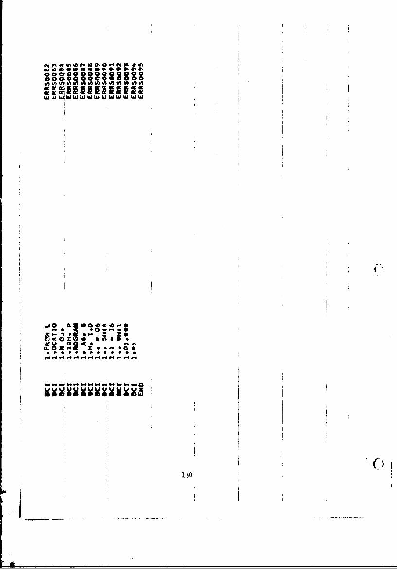
%Att-0 Q % 000M i

aj @30 a.* 0 40a* %0d *4e0~coo

00

130

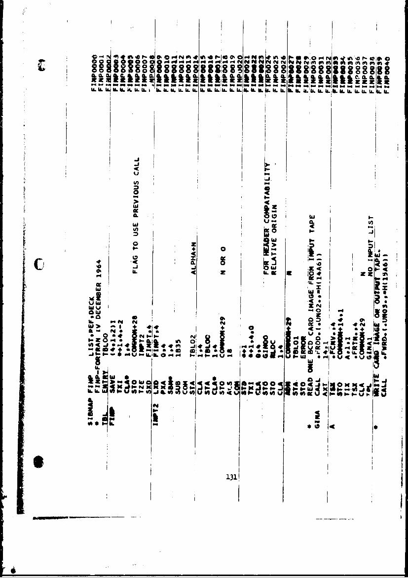
14ZL ~ ~ ~ ~ a.LL~hUI 11liar &MOZ IL kill kil t 11.11,1

LI-

UNO,a 4 wZ4 -4

I JL~

a zU

I I44 -J a 1 t40

Wa

1311

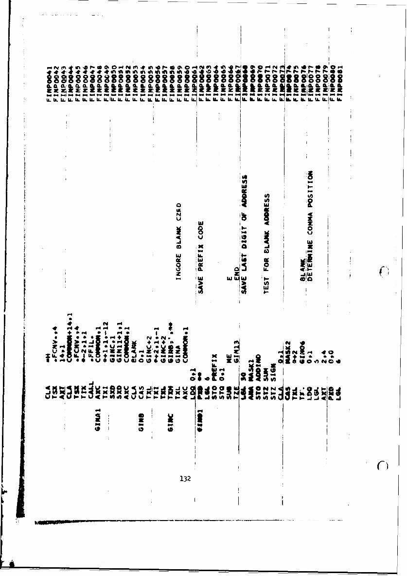
V-0 % O4 NM 4mvtlo O CrNM 0

44 n I

U.

u

4K

"a 0w W #- 4

0 I- 00 U

4q 0 P 0

2 04 04

C 4

IL

.0 .4 60

* e4 ~ -- *p - *J.M +xie4o 1109 d' as

424

13

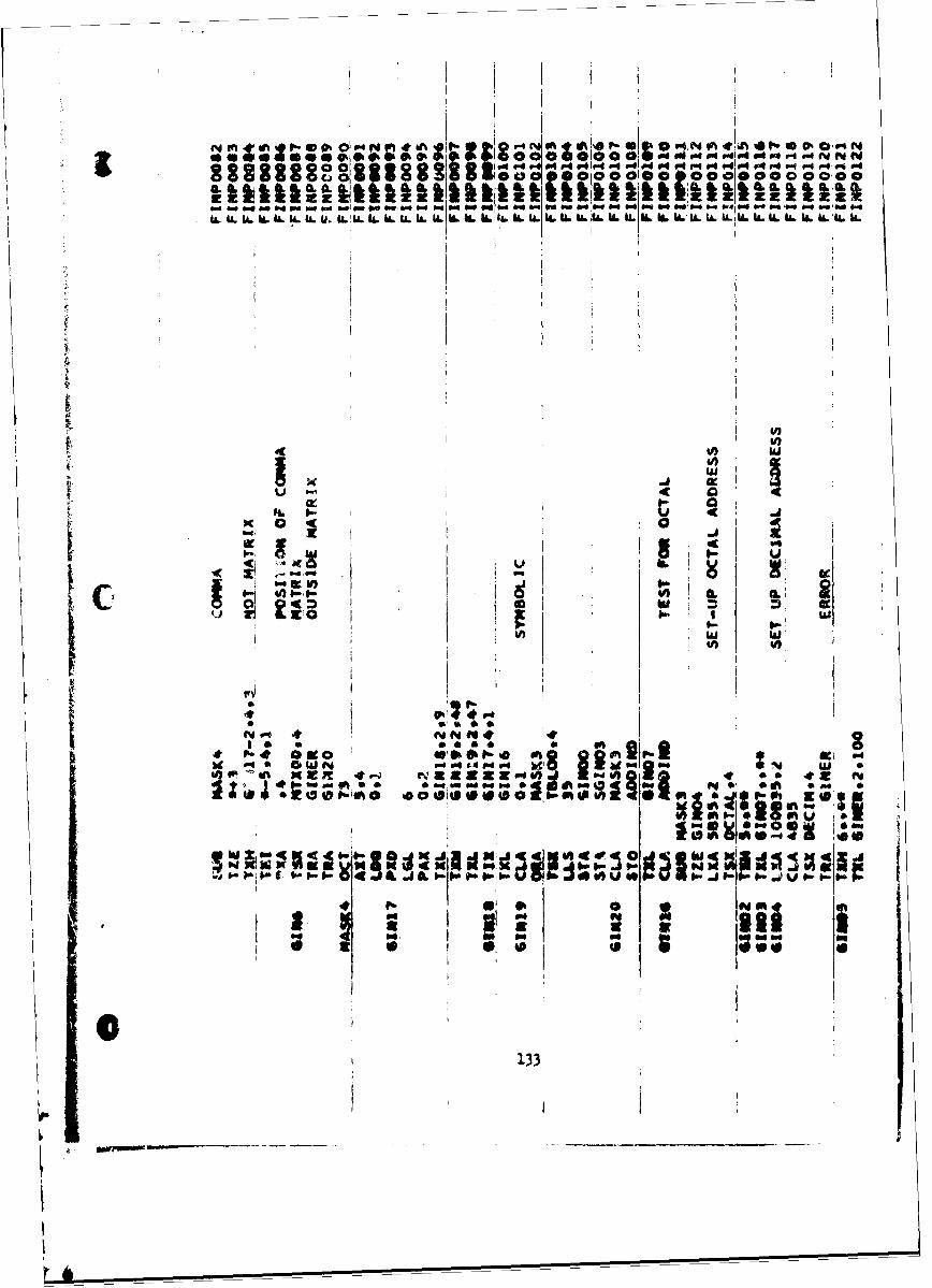
66**0*002 0t1 000 0000--~

10 4 0040 04_" #4 040 04. P1 1.4 #4 04 M 4 0. f-4 4 %

W W

4W

J U,

ofwU

i~.IL

rx 0. 0 -0 P

NoaI O 0 , o n

0s 0 I'i

N~low

I- MltAC I j wIv-a4 I .0v00-1

1.33

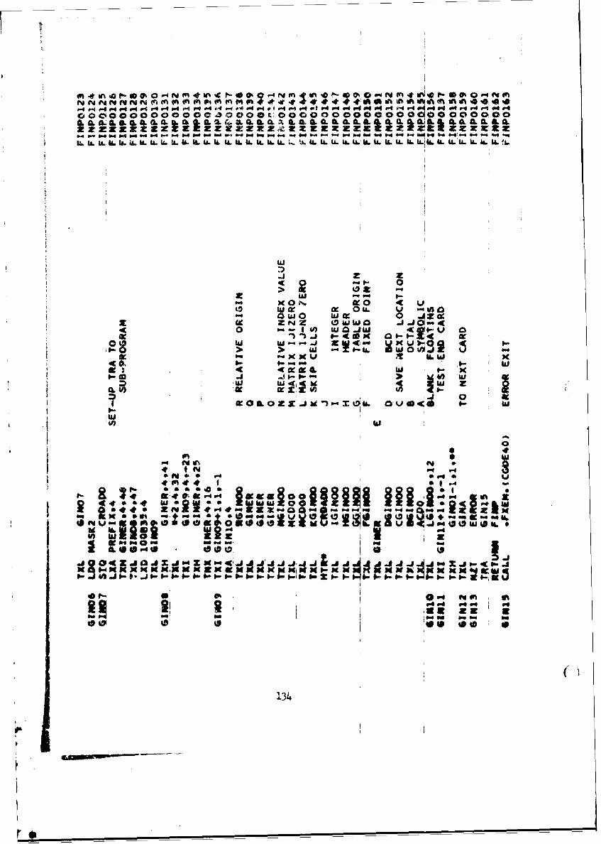
4 -0 4 . . . 1. 4 b - 41 W IW e " 444. "41 ". 0" 641141 "4 444 .- .~ .e a" 1 4

W!W WL WLI . i IL. W i I& WL W L WA W &iL &A. WA WA W~ W44 tu Wi Wi 4 IL IL IL W . W wl. IL U 4 . L IL 11644 IL I.

4 0 1 0

OW W 0 r..iW 0

(9 ZNZ 45 WizJ J j doaoc40 14IU I V)W .JW 4g.v o

6.0 UXX W

ez 4 dc 4wx

J1 V 40) w

0

f tN y

* 4 * r4 *.

a,4h 1620 1 . Z 4 ~ .~~.4 a-

M~~~~~~ ~ p )IM M M g0M~-( W2UIitX 4B

b6 P'04

OF, WI* Z e

a3

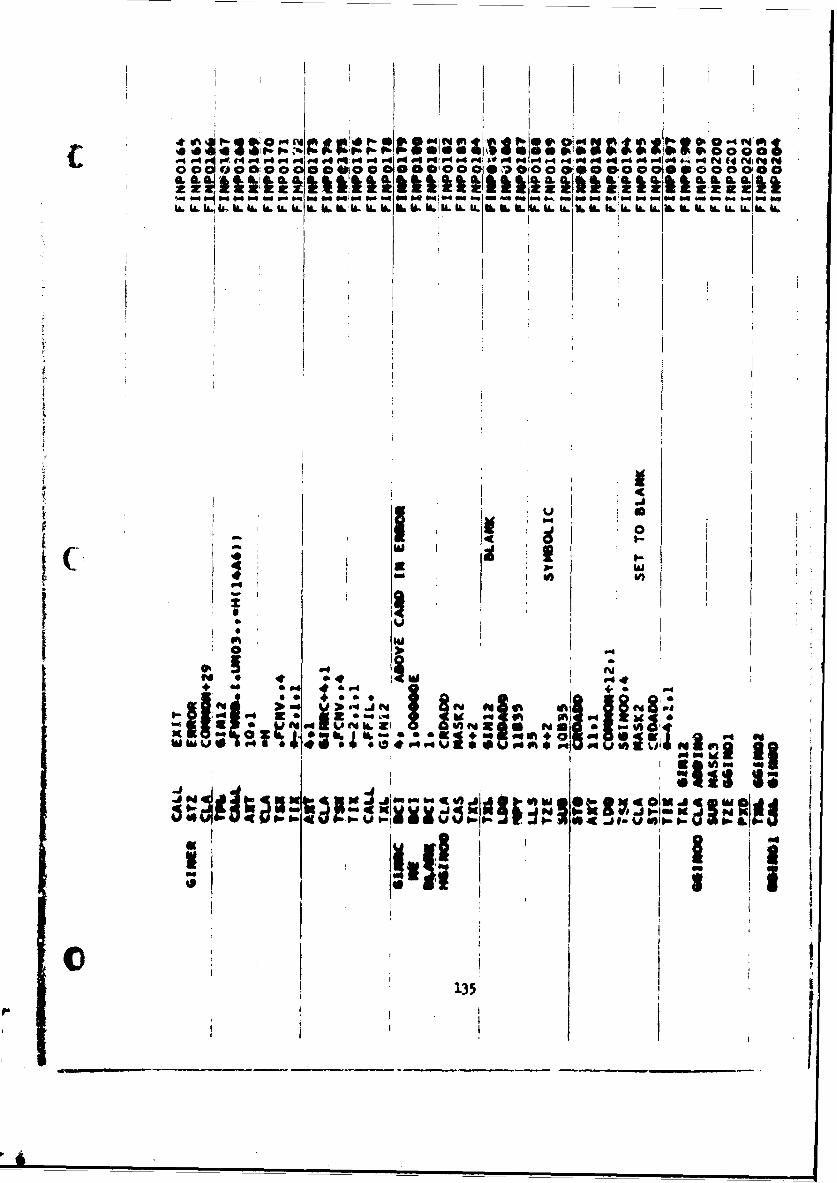
6#@PI P*P4.t (W @0 A4*lF. Utp PON~bSIS It- 0041 ONas O 00 ,09;St9 0000 0

'.4 104* 4p 4f 4e 0~p ~' 44* 44 4 4pe414 P4 4 4. * 4 4 (4 CMN MC000000-000000000 *O@0 0 00000 oooooooo0

WILAI WL6~kS *SOLhM bA.~L~ll~L N.U.. -- A

$-

0 4

+C 60 Soo!:IIavr4h+i0P4

PIA *

C I

135

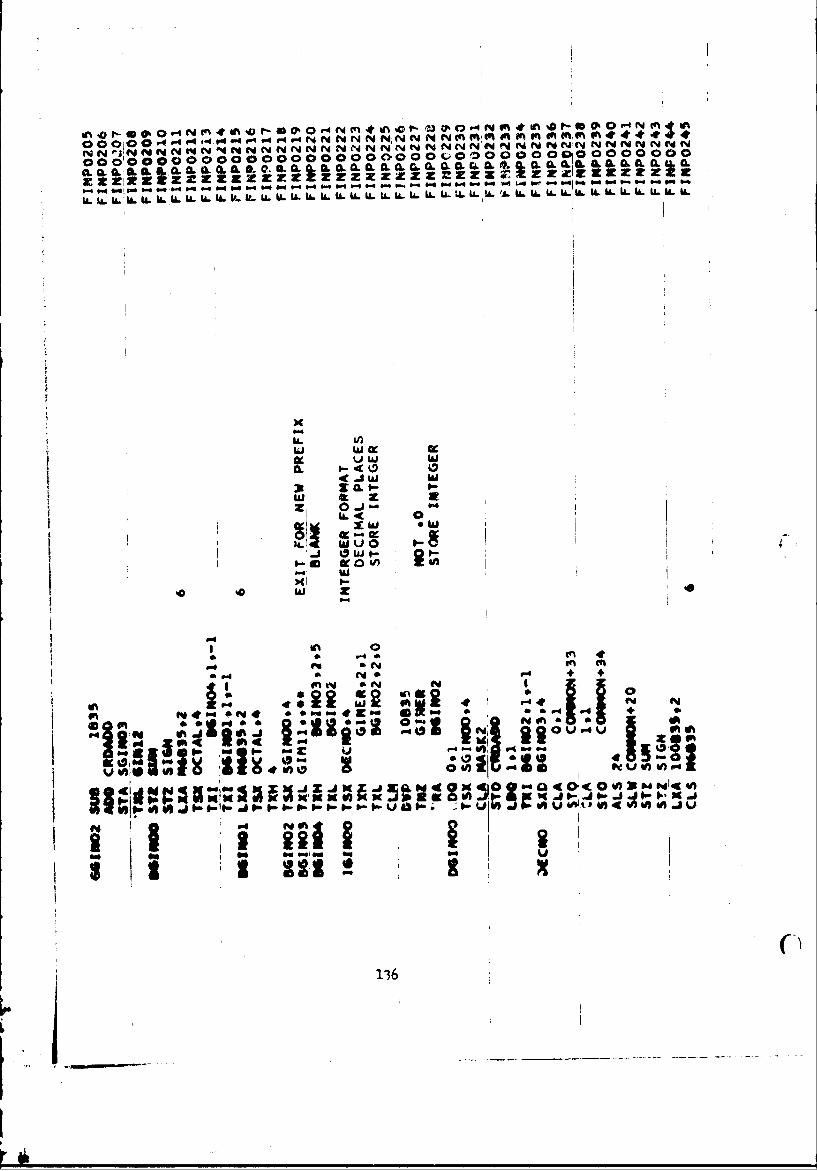
O00,0 0 4 .4.4t4 - '4q '4 4 N Nm I N N 4N N N4 NfyM '%( A A no "m 0111 -It 4p~ s

N N'A NN NN NNcN NN NN N NN N NN N N N NN N N N N N N N N4r Nr N

00,0000000 00000C 000 OCM @0000 00 0

CL I I 1. A .. L A QL L .I A A . L. M A & A M A &'M Ii. &i &L &A ciA. IA. . CA.LA IL I IL 4L I.L. I&. CL .L; IL

I ZI

4I S-S w U

U..A

-wallM

14. N u SN M

5.4 N* 0.4 P.

00

aggin P4j -t- al 'P11 41f 0 N h 0 e Z00 d Ow a a 0.

elm a 00 04 0 0 142 136;O o :II

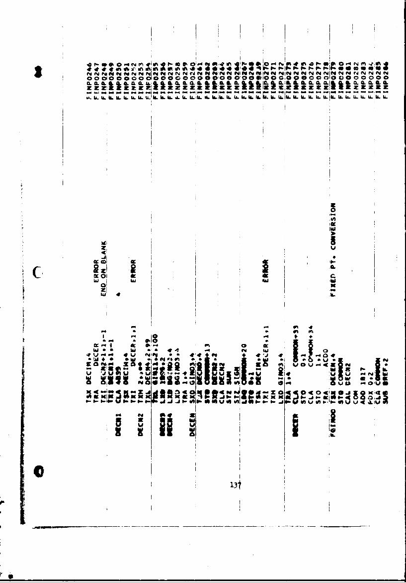
CLCLCL IL0.4U-1 &CLL Mh.I, Ii j161-ILIL I. I. CL QL CLIk. 0-. Q CL: L IL

It

I v

2w w

Nip Al 09 to V0 0 .e f

V I -

131

I oS

0 0 @' @' 0 0'. M' M' 0 U. 0000000000 e4~ 4 - lo44.4.4'-4 iN N NNN NN N

all.0 a. (I1S.a 0. akmilml am al 0.CL a0. &a&0a.a.0zzz z gtzzzz ZZZ1 zzrzztzcIzrztZZrz z~z zzt

--. U. W b LL -U . U -U 14 .L L .'-L.LLL .U .U .U -:

z

0

'I)r

0

U w

-11 z- 0.do ~ ~ 40z -WW4. -

fin-spb-4CAL . UM OZ 19 (C11l& 0ILI. nU N

0 0N .4

AL q4 (4 4

.- eN ~ z *.t4~ a t~r'134t

mmm

z4 t U)

.. z

ix F

thJ 0 c4

-w W

-0 0 a0CN Z A 04 z ZW uj Z &

k + N 30QCK% J a@ltDO as M! -I WLWi-. 0C

U ) 0 U ) M ILO) V. I~~ V) U4( 1 1 ) t q

IIlow.3 itDl 4C a35:V 44 -

j j-j .1 I. I. VU0-U k '- V $ :i ) 4) %J ~ de n 1 I1

139

rzz zaz]iZ xzzzz KZM zr4 "4 50" "" - 0Z. U. L I A z z .LI . . U. U" .. U*' U. i..I. U, W U. W. LL U. W. W. W!U IL W .W W U. LLJt&. LL i. u. U. w: a. 6s.

Lu

0oo0-

4 -z

V) J<U 0 0

0 z

o

'E) Ok

vNP>OZ&ZJ& Z oI~o~v8

I--

0

- *u.4e a .4 0~

00 ~~~I coo 111111!01 oo co~ ~ ~ I 9&. 11 W I&b.I L I~I. IL AL IL W&. b..6AL %. 6IL V .IL I& IL k'

K

-Jz

wI

in tn I

4p -

NEw 00sdff * 1OWSoi W10 VQI.J 0

UO 0.wo 01 0Po01 4 0~ 4 ~ E( 6O A uiWIN a IN9- W N 0 qcA4

VN K N Z4 IOf.X NKd% 0 J

I- 9- uv v

ci a

WON

P4~ C44 0,0 4V

U.. U.~ L . IL IALI. ILIli 1 L I L L IL IL IL~I I I L. U. L 1aM IA IL IA. IL~h 11116 iL IL LI&! wL IL

C9

0c'9 O o O 0 O%0f % U0-4 in1 -

X Go uuuu m0000P- 0 0

I.- -ja i.- S .- 0a .-0 e

IP d%~4 e

v w a 4 ON

w N' 11 Kp. 0 ,1 I W eI J

142

16 wl 11 Vi 112 wU w %6 A.1166 w W1IA I ~& W

I4 I

v 0

nh~I 0 .~ 00iA0.00040 00o M 'VO 0 P

0 n 0a 0 m~ W41111210 i"gem ~ ~ ~ ~ ~ ~ ~ . O 1101P"#In0rt 31 o

IN 0 0 2 J 0g*~~gg~~g.......i .s .~ . . wd c~~

uUUiiUVV UuvvvwUvg "" "v v . ~a~~~0 uJv~ V

SS 9X9v 99aa4

K~I P1 h.fm*

M Pol .

1,3

in a

00000000:9,00 00@@O0@OO@@O 0c @000 @**oHOOo

IiWk kILpi L A.A I L L LILU. Wt.I

11 g1 w9K2

ml IS6' 9

X

0 IOM f0 - t

bi 0.4 1.- 4 1 V 1~v CID 0+

0

vK 0

v(

-" j -"-" - :".. . . *''''' '

I I

I

IA

iin

I 00

MM

i

qf~4% - O j

W . LV .baUI .w U.I L LI IL U .. 16 16 ILI LWW0 6 L I L

• -Q

4L

1~J1

__________________P4________

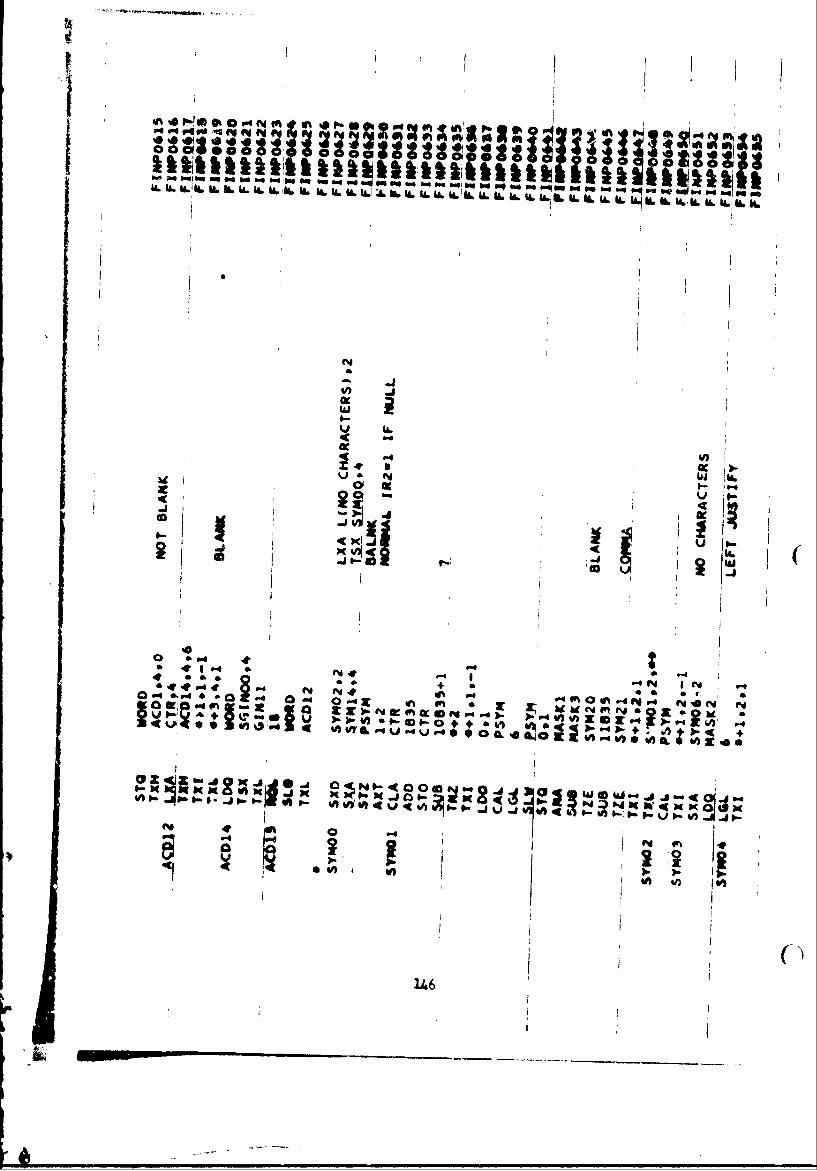
00.1

a

4c

W-4p30

coo

0~~ .p4 -C

P-

v q-nN w

4

146

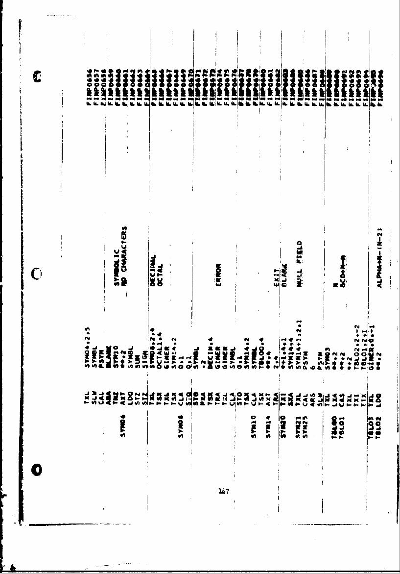
I

I, I I Ii.

j

log- x j J IP, Z,-

S10 CDI '

94I W A N..

ot, t4' . U .4-- 04 4

04ft ftM g

147

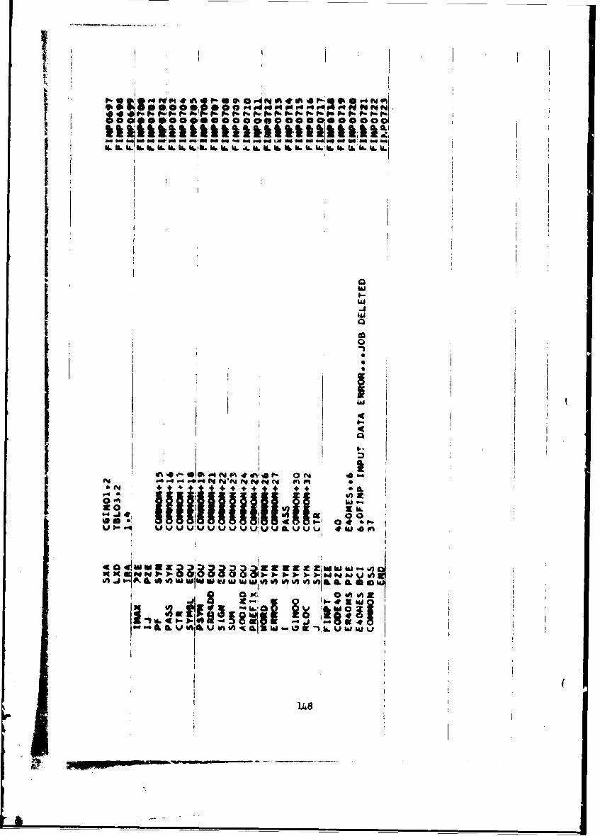
t- 0 I4M4 400 p^ 10 m o~ o # o * ~

p.. *r4001000090d0004r

4L OL W, p U. WAL I .L U.1116 IL U-11.~~

'U

A

90 M 4 On'si1- kiNzK 00

.- I vI W~jWvvjt v 4# W MA I I IV I

14'8

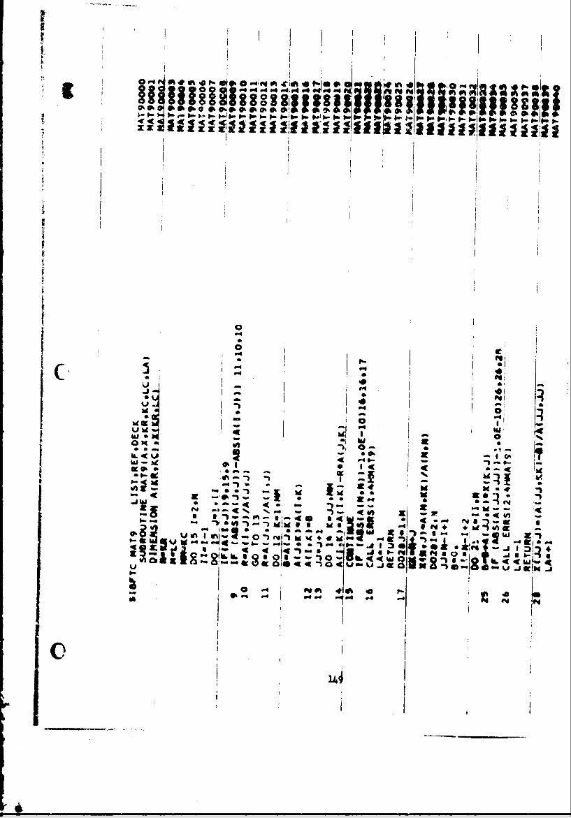
z z

ff 0

i ID

I a 7 aweon -. 4 , Ot0. f

OK ;

E -A I-O, 0 - a'I

I. V - £ a

rz

150

W 4 F0

'i

W 0 a

t0 O 3

N""da*4

"Rwl

I15

t

dc-

IxN

0-

U . mi 4~

0 &I

ac, x4I~

10 x.

acqc u. ra- T 'C 0-t"

0'- 0 of 4

21( & 00 *4tV) hI V) a1 z fzzZ% 0

-' wN 0 a- LI 1

I I"l D wOi Zn 0 0-01 C ON

w~~ ~ ~ .A t44 owee

P.. -Y aK 1, '4 .

WZ~v 4J a- u 4 wi

~4 Ba N.E L '4 W52

"~ Ik

2x IW

-C [%of Pocp

oft .0a -00 i

.- C

x'0 1 3

Ot

a0. a %W P- P4 ft r

.15

I i

.j z

IV a

115

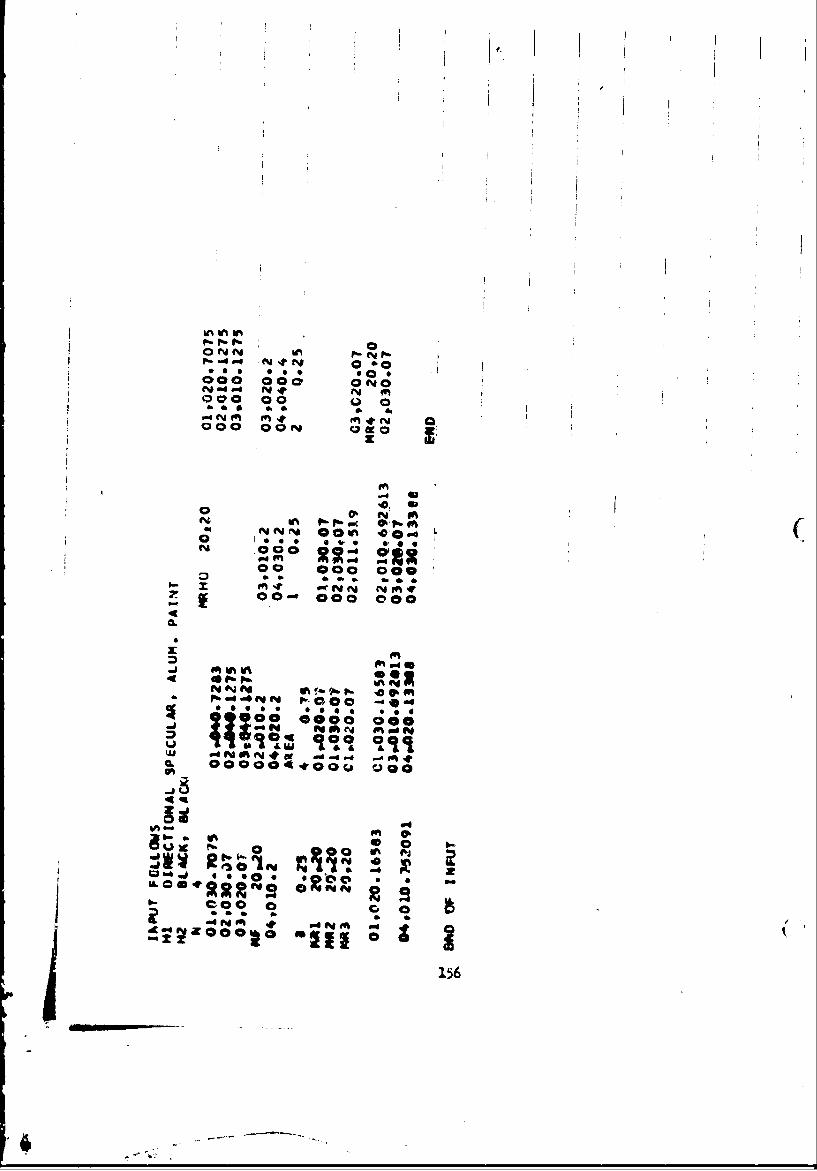
C00

000 O0r

~04:

o0 0

0 h 00 coo

f"'~ Vw A0 '0 Fft 000

Pi 0 @0 0 00

I- ~ 0 f ~ t MANE'~ mI00-ao 100 0i0

4LI

0 9

I, a'mt OdU

15

I K

z 44

I IU, I

N I

o157

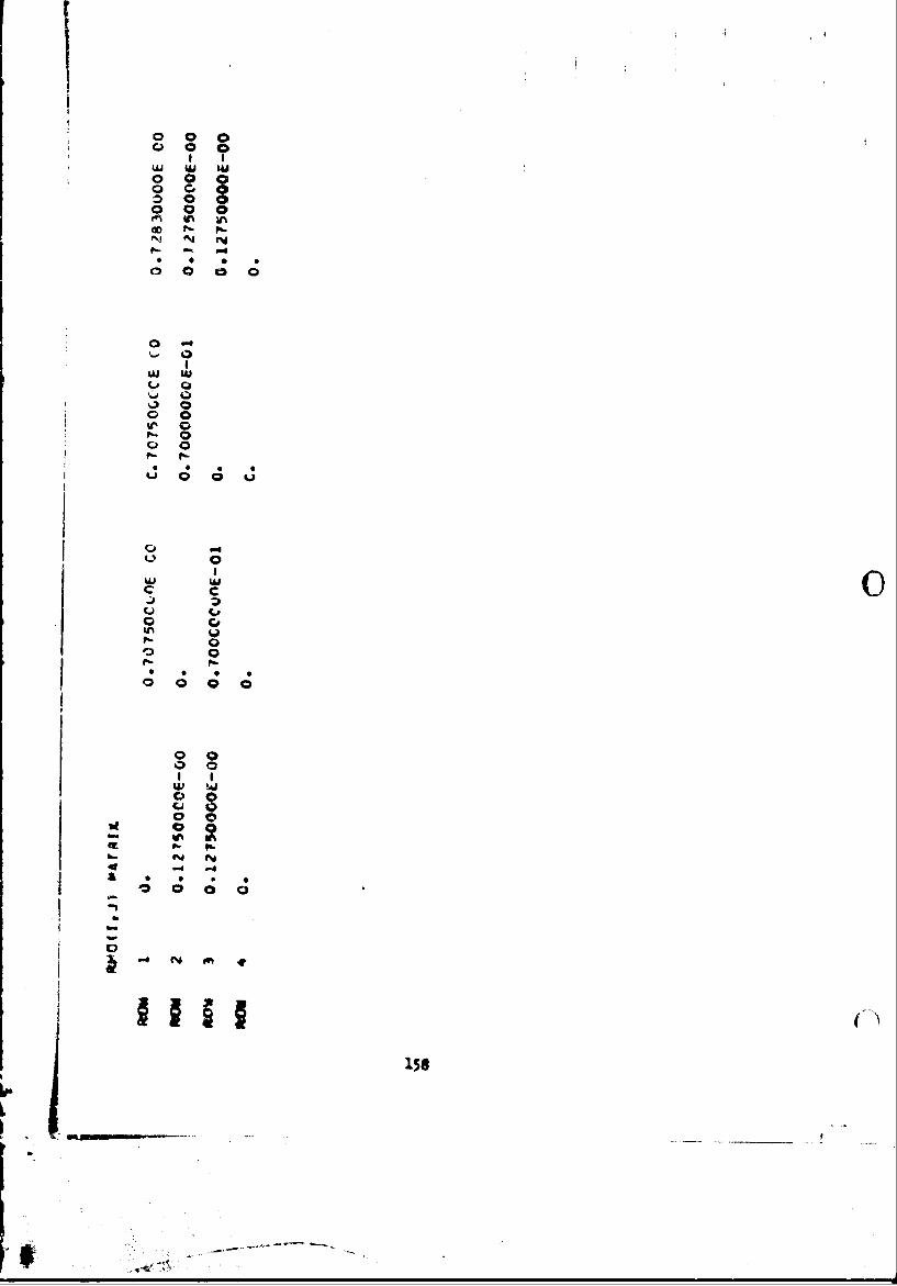
00

w w- iu

00

C? C'

Sp-

c c

o

0

w wQ0

ob0

40J 0; a a

C,158

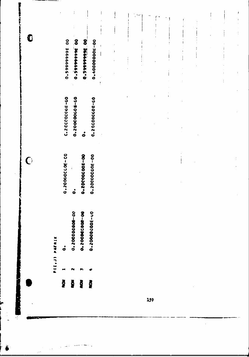
W~ uj

000

400Ica

ft0

15

cl

oi

o

16

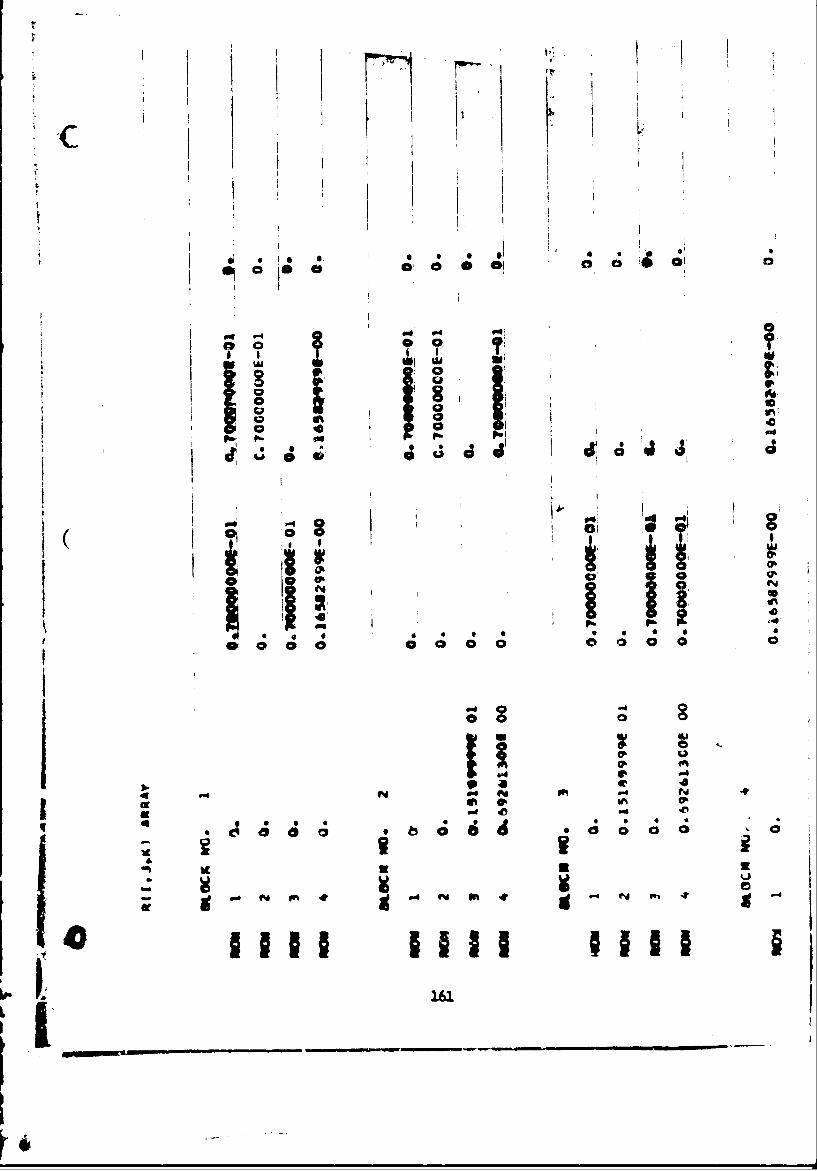
I0,

ICP

* * IP

cc Sc

on

Im o

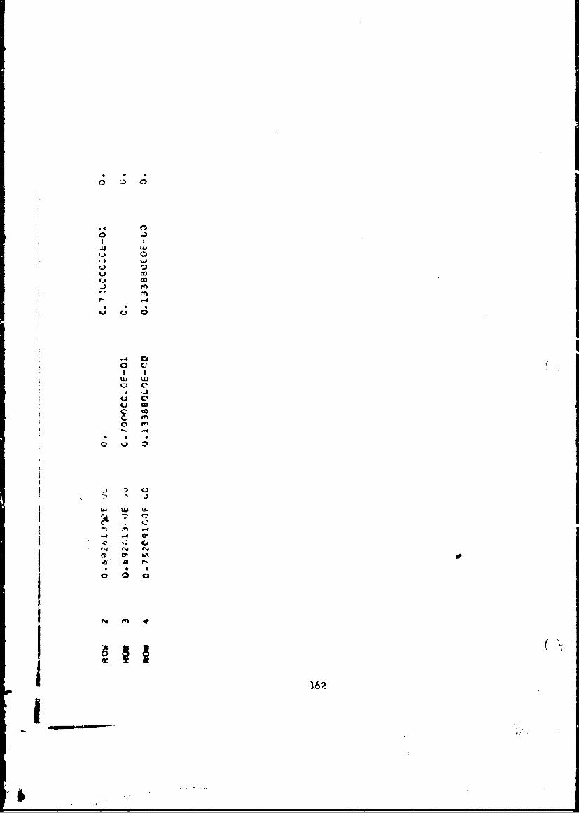
o 0 40

0ey

A

ry f

* 1.62

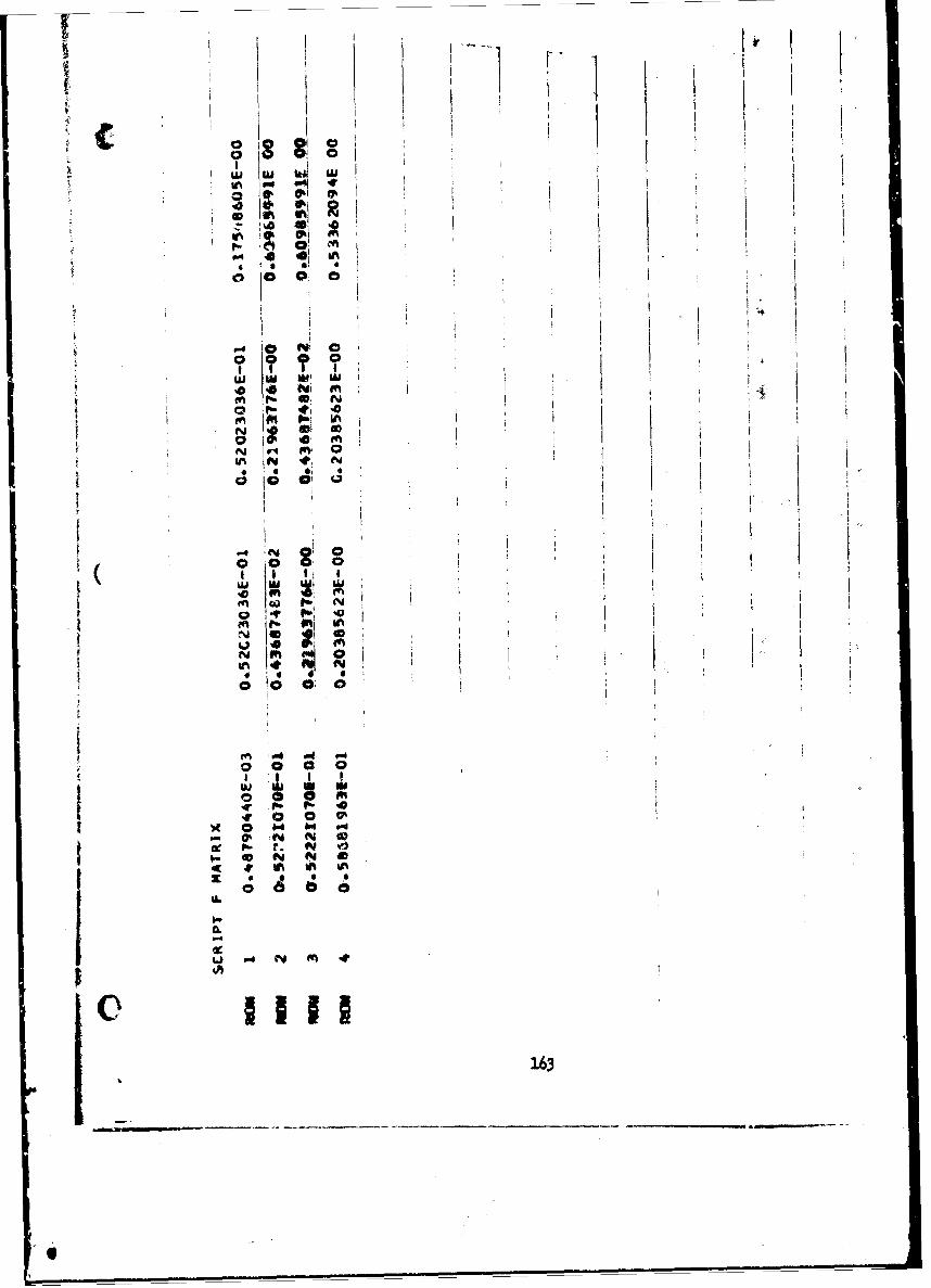
! W

I '400

1 0 m

w 0 " m

* g tV I

o % N

U-L

atI163

U.'.

.'vI I I 1

i ... fN IrI m - " - - - -I - . . . . I[I

- ""- - ...

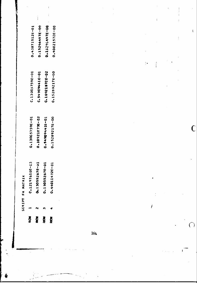
AAwU w I" wU0N CP P~-

14 o ~

*- V4 O 0

Q N R 0

WU w~ UL

P- M in P~

I I I C

n - 0 0

I~'~ 0 4.164

APPENDDC IV

EXPERDMENTAL DATA-

RADIATION EXCHANGE EXPERIMENT

165

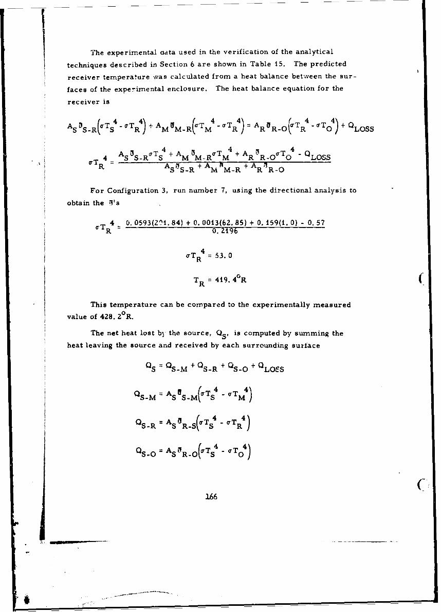
The experimental data used in the verification of the analytical

techniques described in Section 6 are shown in Table 15. The predicted

receiver temperature was calculated from a heat balance bet-ween the sur-

faces of the experimental enclosure. The heat balance equation for the

receiver is

AS SR(~Ts 4 - OTR4 ) + AM 4M)R(oTM -OTR)= AR o(cTR - iTo 4 ) + -LT 4

A~ (aT o T +A T +A ~ uT a

or 4 S S-R S M M-R M R R-0 0 LOSSAS S_ + A 'R + AR1 OAS SR M M-R R R-0

For Configuration 3, run number 7, using the directional analysis to

obtain the 's

afT4 = U.0593(2"1. 84) + 0. 0013(62. 85) + 0.159(l. 0) - 0. 57R 0. Z196

4uTR = 53.0

TR = 419.4°R :

This temperature can be compared to the experimentally measured

value of 428. 20 R.

The net heat lost b) the source, QSP is computed by summing the

heat leaving the source and received by each surrounding surface

Q = QS-M + 0S-R + QSO + QLOS

~S-M AS 5M(7T 7TNS -4 M4 )

0 SR S ~ (cT 4 -r uT 4 )

_so A~ O(T 4 or T 4 )

166

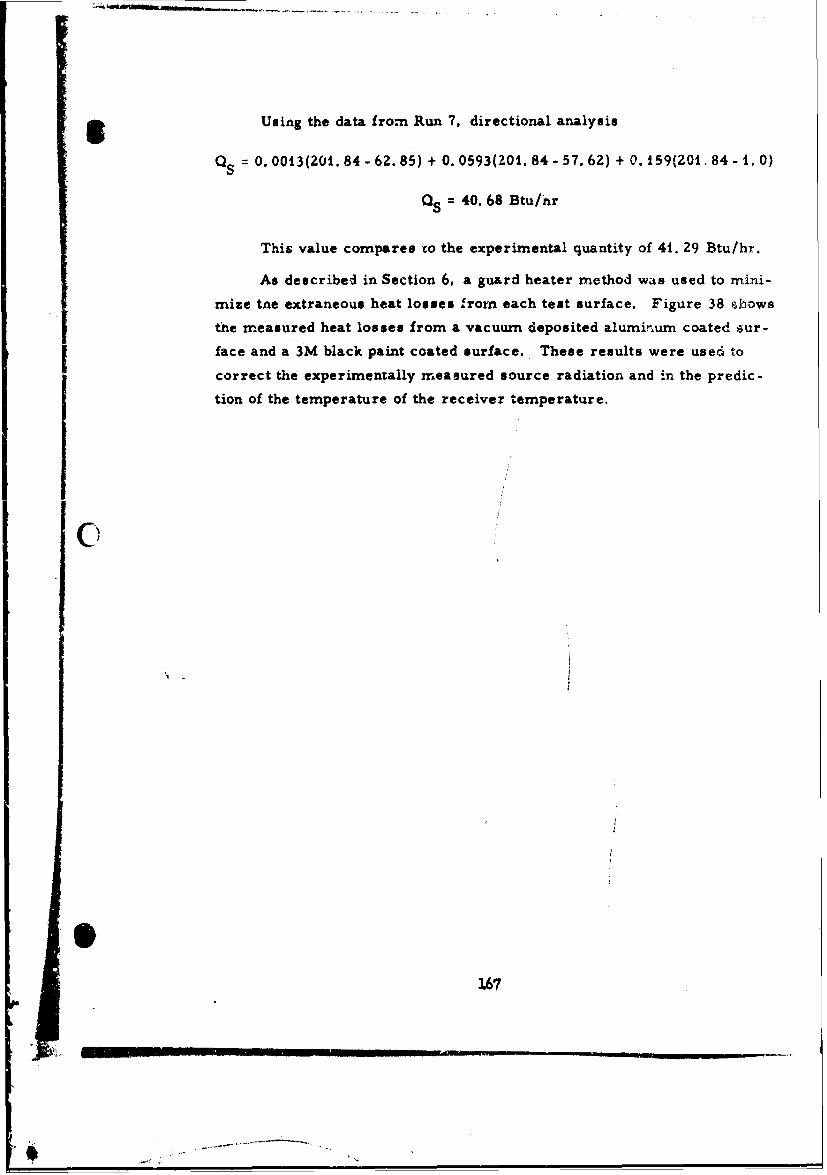
gUsing the data from Run 7, directional analysis

Q = 0. 0013(201. 84- 62.85) + 0. 0593(201. 84- 57. 62) + 0. 159(201, 84- 1. 0)

QS = 40.68 Btu/hr

This value compares to the experimental quantity of 41. 29 Btu/hr.

As described in Section 6, a guard heater method was used to mini-

mize tne extraneous heat losses frorn each test surface. Figure 38 shows

the measured heat losses from a vacuum deposited aluminum coated aur-

face and a 3M black paint coated surface. These results were used to

correct the experimentally measured source radiation and In the predic-

tion of the temperature of the receiver temperature.

1

I -

/6

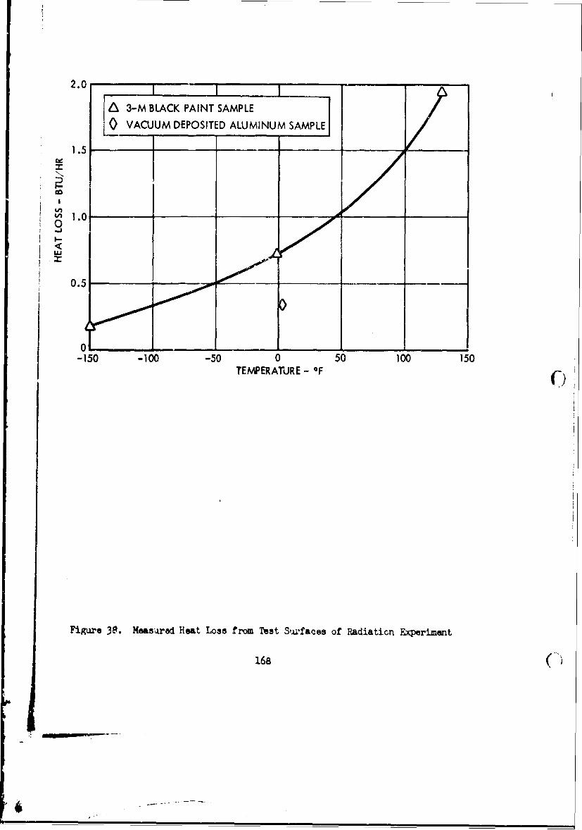
2.0 7 -__ _ _ _ _ _ _ _ __ _ _ _ _ _ _ _ _ _

A3-M BLACK PAINT SAMPLESVACUUM DEPOSITED ALUMINUM SAMPLE]

1 .5

O.0

05

-150 -100 -50 0 50 100 150TEMPERATURE - O

Figure 38. Msarad Heat Loss from Test Sur~faces of Radiaticn Experiment

168

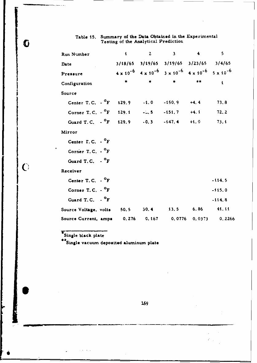
Table 15. Summary of the Data Obtained in the ExperimentalAr Testing of the Analytical Prediction

Run Nunber 1 2 3 4 5

Date 3/18/65 3/19/65 3/19/65 3/23/65 3/4/65

Pressure 4x O 6 4x t0 6 3x 10 6 4x 10 6 5 x 10 - 6

Configuration * * * ** i

Source

Center T.C. - OF 129.9 -t.0 -t50.9 +4.4 73.8

Corner T.C. - OF 129.1 -.. 5 -151.7 +4.1 72.2

Guard T.C. - 0F 129.9 -0.3 -147.4 +t. 0 73.1

Mirror

Center r.c. - OF

Corner T.C. - 0F

Guard T.C. - OF

C Receiver

Center T.C. - 0F -i14.5

Corner T. C. - OF -I15.0

Guard T.C. - OF -114.8

Source Voltage, volts 50.5 30.4 13. 5 6.86 41. 1I

Source Current, amps 0. 276 O. t67 0. 0776 0. 0373 0. 2266

Single black plate*Single vacuum deposited aluminum plate

169

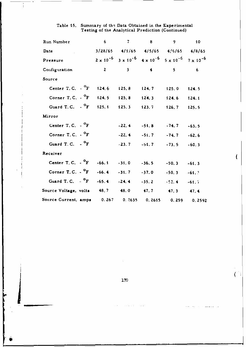
Table 15. Summary of th-! Data Obtained in the ExperimentalTesting of the Analytical Prediction (Continued)

Run Number 6 7 8 9 10

Date 3/28/65 4/1/65 4/5/65 4/6/65 4/8/65

Pressure 2 x 10 6 3 x 10 - 6 4 x 10 - 6 5 x 10 - 6 7 x 10 - 6

CoiJiguration 2 3 4 5 6

Source

Center T. C. - 0 F 124.6 125.8 124.7 125.0 124.5

Corner T. C. - 0 F 124.5 125.8 124.3 124.6 124.1

Guard T. C. - F 125.1 125.3 123.7 126.7 125.5

Mirror

Center T. C. - 0 F -22.4 -51.8 -74.7 -63.5

Corner T. C. - F -22.4 -51.7 -74.7 -62.6

Guard T. C. - 0F -23.7 -51. 7 -73.5 -60.3

Receiver

Center T. C. - OF -66.1 -31.0 -36.5 -50.3 -61.3

Corner T. C. - 0 F -66.4 -31. 7 -37.0 -50.3 -6t.'

Guard T. C. 0 F -65.4 -24.4 -35.2 -5. 4 -61.,,

Source Voltage, volts 48.7 48.0 47.7 47.3 47.4

Source Current, amps 0.267 O. Z.635 0.2615 0.259 0.2592

170

APPENDIX V

BIBLIOGRAPHY FOR

JOINT THERMAL CONDUCTANCE

173.

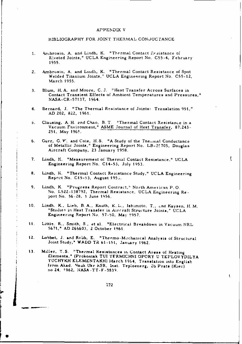
APPENDIX V

BIBLIOGRAPHY FOR JOINT THERMA.L CONL)UC'rANCE

1. 4rbrosio, A. and Lindh, K. "Thermal Contact Rr~-.sistance ofT

Riveted Joints," UCLA Engineering Report No. C55-4, February1955.

2. Amnbrosio, A. and Lindlh, K. "Thermal Contact Resistance of SpotWelded Titanium Joints," UCLA Engineering Report No. C55-12,March 1955.

3. Blum, H. A. and Moore, C. J. "Heat Transfer Across Surfaces inContact Transient Effects of Ambient Temperatures and Pressures,"NASA-CR-57137, 1964.

4. Bernard, J. "The Thermal Resistance of Joints: Translation 951 ,"AD 202, 822, 1961.

5. Clausing, A. H. 2'nd Chao, B. T. 'Thermal Contact Resistan(ce in aVacuum Fnviroinent," ASME Journal of Heat Transfer, 87.243-251, May 1965.

6. Gurr, G. W. and Cote, H. S. "A Study of the Thei mal Conductanceof Metallic Joints," Engineering Report No. LB-21_705, DouglasAircraft Company, 23 January 1958.

7. Lindh, It. "Measurement oi Thermal Contact Resistance," UCLAEngineering Report No. C14-53, July 1953.

* 8. Li;ndh, KC. "Thermal Contact Re3istance Study," UCLA EngineeringRepor~t No. C15-53, August 195J.

* 9. Lindh, K. "Progress Report Contract," North American P. 0.No. L522-138792, Thermal Resistance, UCLA Engineering Re-port No. 56-28, 1 June 1956.

10. Lindh, K_, Lieb, B. A., Knuth, E2. L., Ishimoto, T., ,fLnd Kaysen, H. M,"Studier' in Heat Transfer in Aircraft Structure Joints," UCLAEngineering Report No. 57-'50, May 1957,

It. Little, R., Smith, S_, et al. "Electrical Br' ,akdown in Vacuum NRL567t," AD 26660), 2 October 1961.

12. Lobbet, 3. arid Robb, E. "Thermo -M,!chanical Analysis of StructuralJoint Study," WADD TR 61 -1t51, Janua ry 1962.

13. Miller, Y. S. "Thermal Resistances ir. Contact Areas of HeatingElements," (Prokontak TUX TERMICHNI OPORY U TEPLOVYDILYAYUCHYKH ELEMENTAKH) March 1964, Translation into Englishfrom Air-ad. Nauk IUkr RSR, Inst. Teploenerg. Zb Prats (Kieu)no 24, 1962, 1-ASA-TT-F-3839.j 172

IVO.

APPENDIX VI

COMPONENT JOINT TEST DATA

USZD FOR CORRELATION TASK

173

Three experitnental tests~ were ccmducteL4 to verify t-- .esult-i of

tie cortktion ta~3k P,,-r experimenltal me- surernen- are given in

Table 16 The tberrnocouole locations and dat;. reduction tt-chnique are

described in Appendix I.The bolt location,- for these three tests are

Phr.,n Ln Figu re 39.

174

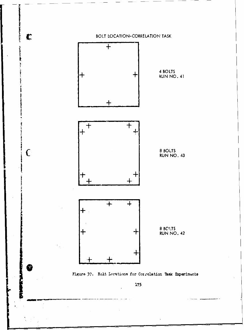
BOLT LOCATION-CORRELATION TASK

4 BOLTSRUN NO. 41

+ 4-+

i I

I8 BOLTSRUN NO. 43

+ 4.

Figure 30. Bolt Ircqitionn for Correlation Task Experiments

175

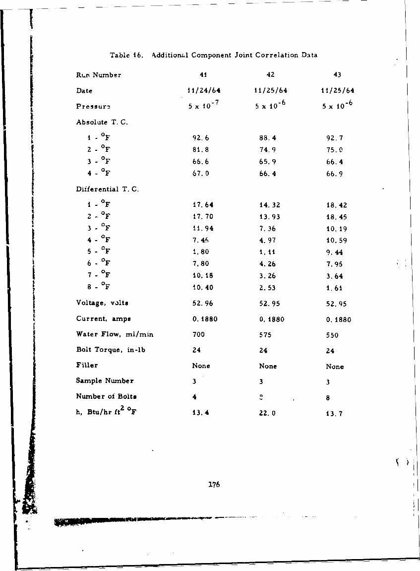
TTable 16. Additional Component Joint Correlation Data

Rur Number 41 42 43

Date 11/24/64 11/25/64 11/25/64IPressuri 5 x 10- 5 x 10- 6 5 x 1-

Absolute T. C.

Si- OF 92.6 88.4 92.7

2 - OF 81.8 74.9 75.0

3 -0 F 66.6 65.9 66.4

4 -0 F 67.0 66.4 66.9

Differential T. C.

1 - OF 17.64 14.32 18.420

2 - F 17.70 13.93 18.45

3 - OF 11.94 7.36 10.19

4 - OF 7.46 4.97 10.59

5 - OF !.80 1.11 9.44

6 - °F 7.80 4.26 7.95

7 - °F 10.18 3.26 3.64

8 - OF 10.40 2.53 1.61

Voltage, volts 52.96 52.95 52. 95

Current, amps 0. 1880 0. 1880 0.1880

Water Flow, mllmin 700 575 550

Bolt Torque, in-lb 24 24 24

Filler None None None

Sample Number 3 3 3

Number of Bolts 4 2 8

h, Btu/hr ft2 oF 13.4 22.0 13.7

176" 176

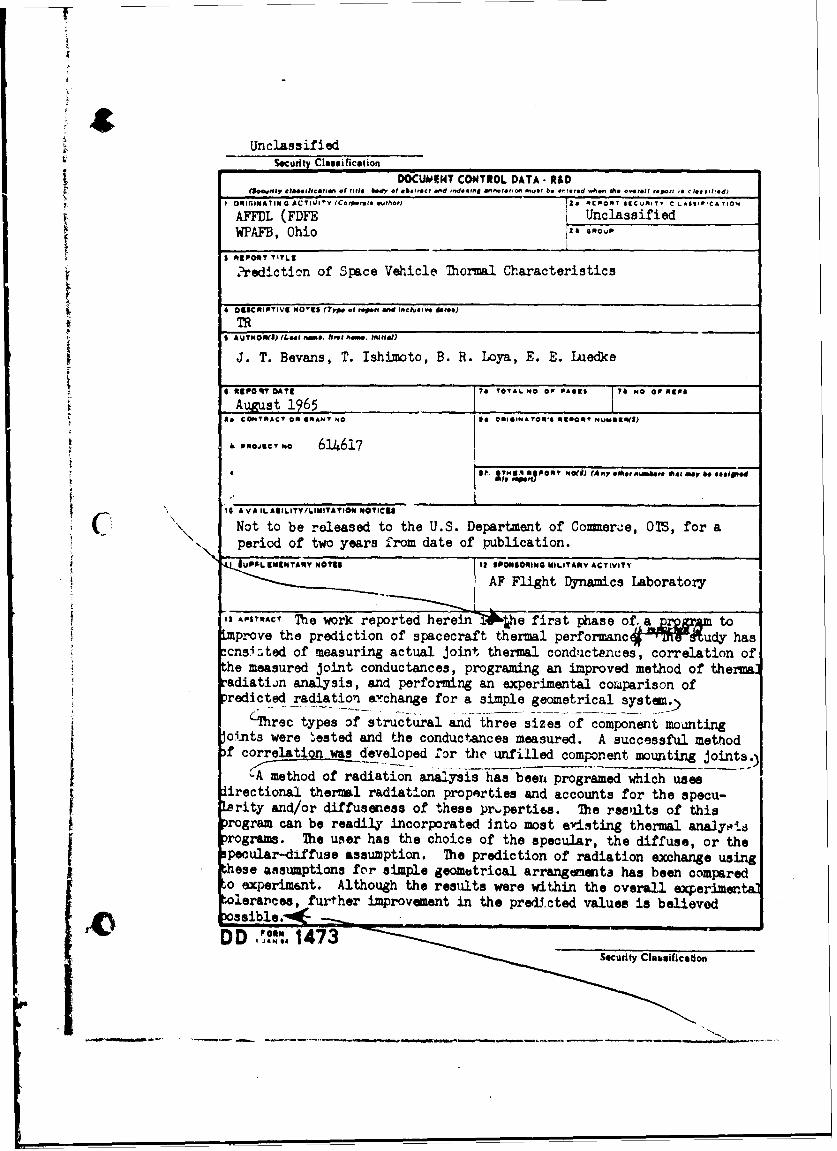
Unclassifiedsecuulty Classification

DOCUAWqHT CONTROL DATA - R&D(aeuvty02 s fia. ifee~uos .fit. e t Of ob.tr*cr And *nd*.sn orn~fo .I g. - . . r. I . IA fth e "01 els- Is eI..e11ftill

I ORIflIMATIl 0 ACTIVIVY (C.,o,.'*ii outh@*J 2 COT SKC RITY C LASl WICA !ION

AFFDL (FDFE Ia UncloassifiedfWPAFB, Ohio 126 GROUP

I WRIOT 'lYLE

2redicticn of Space Vehicle 31hormal Characteristics

4 OESCRIPTIVI N051N (Typo o1f reor ad Inlusive, dittes)

TR6 AUTHOR(S) (Last Item. hist Roe, iitial)

J. T. Bevans, T. Ishimoto, B. R. Loya, E. E. Luecile

S REPO UT DATE 7 TOTA6 NO 0F 00699 71 O OPRaps

August 196Of CONTRACT ON GRANT NO Of ORI6I4NATOR'S ARORT NUMDER(S)

PRO~eT Wo 61.4617

aS A VAIL AILITY/6IMITATION NOVIC9S3*0i Ay*111hSSa pb eig(7 'KNot to be released to the U.S. Department of Comeroe, 02S, for aperiod of two years from date of publication.I PFIEETR NOa 071 12;1 001104101 MILITARY ACTIVITY

AF Flight Dynamics Laboratory

ii PS'RCTThe work reported herein hefirst phase of. aprove the prediction of spacecraft thermal performanc IEM a

cnsji;ted of measuring actual joint thermzal conducte.nes, correlation ofhe measured joint conductances, programing an improved method of thermaladiatijn analysis, and performing an experimental com~parison ofredicted radiationl &-ichange for a simple geometrical system.)

C~hrec types of structural and three sizes of component moa~ntingJoints were 'tested and the conductances measured. A successful method)f correlation was developed Zor the unfilled component mounsting joints)

~A method of radiation analysis has beent programed which usesI irectional thermal radiation propmrties and accounts for the specu-rity and/or diffuseness of these prpertihs. The results of this

rogram can be readily incorporated into most e'!isting thermal ana~gV'tarograms. The user has the choice of the specular, the diffuse, or thepecular-diffuse assumption. The prediction of radiation exchange using

ese assumptions for simple geometrical arrangemenvta has been compared0 experim~nt. Although the results were within the overall experimentaoleraroes, further improvement in the predicted value is believod

DD ,OM1473 ________

Security Cluasification

"C"It C "'fiat

-....-.-.. '-.- - - - - - - -...

becurity Classification_______

14 KEY WORDS LINKSLN LINK C

1. Space vehicles.j

2. Passive teaiperature control system.

3. Radiant heat transfer.

4. Thersal coiductance of joints.

INSTRUCTIONS

1. ORIGINATINCG ACTIVITY: Enter the name and address imposed by security classificatc-rn, using standard statementsor the cont ractor, subcontractor, grantee, Department 3f Cc- such at,tense activity or other organization (corpiorate author) issuing (1) "Qualified requesters may obtilin copies of thisthe report. report from DDC. "2o. REPORT SECURITY CLASSIFICATION: Enter the ov~er- (2) "Foreign announcement and dissemination of thisall security classification of the report. Indicate hottler

Retstticted Date" is included. Marking is to be in accord- report by I)DC is not authorized,"ance with appropriate securiti regulations (3) "U. S. Government agenc'es mas obtain copies of

this report directly from IIOC Other qualified DDC2b. GROUP: Automatic dosu'tgradtng sis spec'fied in DoD Di uif se; eI request thro.tractive $200. 10 and Armed Frrelt Indastrtal Manuel. kr'trthe group nunbvr. Atila, whent applicable, show that optionalmarkings have been used for Grout I anid Group 4 as auth( r- (4) "U. S. ilitary agencies may obtain copies of thisised, report directly from DDC. Other qualified usees

3. RNWORT TITLE: Eiter the complete report title in all 1 shall request throughcapital letters. TiItle in all costs should be uncloasified.It a meaningful title cannot he selected without cl.,ssifuica-tion. snow title classification in all pitisis in jarprnttesis (S) "All i,* ubution of this repo'rt is controlled Qtaaimmediately followi.ay the title, ied DDC users shall request through

4. DESCRIPTIVE NOTES., It appropriate, enter the type of ___________________

report. e.g., interim, progress, summary. annual, or final. If the report has been furnuisherd to the Office of TechnicalGive the inclusive datest when a specific reporti ng period is Services. Department of Comm~erce. for sate to the public, in.lcovered. ", ca this tact and enter the pr'co, if kr ownS. AUTHOR(S): Enitir the name(s) of author(s) oa showv on It. SUPPLEMENTARY NOTES: Use for additional explana.or In the report. Enter lost nameu, first name. middle initial, tory notes.If .miiary, she- rank and branch of service. The name ofthe principal , 'thor is an absolute minimum requirement. 12. 5PON30RING MILITARY ACTIVITY: Enter the nme of

1% a Ithe departmental project offitce or laboratory sponeoaring rpm.&. REPORT DATE.. Enter the date of the ratiort day, Ing f1r the ro.osrr-, in' 41 dolfnlopmesi. Include address.

month. year; or month. year. If more than one date appears 3AS"RC:Eeraabtatgvnabifadfculon the report, use date of publictation.3A3rAT nri nasrc iig r# n ata

TOTA NUBER t PGES:Thetota pae cont umm.'rv 4 the document indicsitive (if the report, even though I7a. it macy also appear elsewhere in the body of the technical re.,

should follow normtal pagination procedosas. i.e., enter the IPort. If additional apace us required. a continuation shoet shall*number of pages containing Information. be attached.

7b. U~E OFREFRENC& Eter' . 1011 nmbe of I! is highly desirable thai the abstract of clarratied reportsreferences cited ini the report, be unclaa-:ifiod. Each paragraph of the abstrott shill end with

11m CONTRACT OR GRANT NUMBER: If iepprnpriate. enter on inaikalion of the military security clasifirsatiorn of the in.the applicable number of the contract or grant undor which formation in the paragraph, represented ai fs (7' (si. (c). er (1/).the report was written. Thert is no limitation on the length of the abstract. How.Sb, 11c Isi Id. PROJECT NUMBEZR: Enter the appropriate eve, the suggested length is from IS0 to 225 words.militarv departrat identification, such as project number, I E OD:Kywrsaetcnclymalgu emsubproject mnttb, system numbers, task number, etc. 1 E OD:Kl od r ehial aetgu em

or short phrases that characterize a -sport 'and may be used asgo. ORIGINATOPIS REPORT NUMBZR(S); Easter the offi- in It), entries for catalogtng the report Key words must becial rrport number by which the document wi!l be identified selected so that no security classification is requited, Identi.and c~ontrolled by the originating activity. This number must tiers, such asl equipment model designation, trade noame, military,be unique to thie repoet. project codar name, geographic location. may be usetrd as key9b. OTHER REPORT NUMBER(S): If the report has been *ords hut will be followed by an indication of technical con-iaignod any other repear timbers (either by the irirjjitor text. The assignment of links. rules, and woeghts 1it optional.or by the aponso.o), .lso enter this numbirts),to, A VAILARILIT Y/ LIMITATION NOTICE&: Enter any lin.italions on fuvrtoer diarromlnati'. of the report, othar than thosej Security CI8mgffication