Embed Size (px)
Citation preview
TO APPEAR IN IEEE TRANSACTIONS ON SOFTWARE ENGINEERING 1
Matching and Merging of VariantFeature Specifications
Shiva Nejati, Mehrdad Sabetzadeh, Marsha Chechik, Steve Easterbrook, and Pamela Zave
Abstract—Model Management addresses the problem of man-aging an evolving collection of models, by capturing the re-lationships between models and providing well-defined oper-ators to manipulate them. In this article, we describe twosuch operators for manipulating feature specifications describedusing hierarchical state machine models: Match, for findingcorrespondences between models, and Merge, for combiningmodels with respect to known or hypothesized correspondencesbetween them. Our Match operator is heuristic, making useof both static and behavioural properties of the models toimprove the accuracy of matching. Our Merge operator preservesthe hierarchical structure of the input models, and handlesdifferences in behaviour through parameterization. This enablesus to automatically construct merges that preserve the semanticsof hierarchical state machines. We report on tool support forour Match and Merge operators, and illustrate and evaluate ourwork by applying these operators to a set of telecommunicationfeatures built by AT&T.
Index Terms—Model Management, Match, Merge, Hierarchi-cal State Machines, Statecharts, Behaviour preservation, Vari-ability modelling, Parameterization.
I. INTRODUCTION
Model-based development involves construction, integra-tion, and maintenance of complex models. For large-scaleprojects, modelling is often a distributed endeavor involvingmultiple teams at different organizations and geographicallocations. These teams build multiple inter-related models,representing different perspectives, different versions acrosstime, different variants in a product family, different develop-ment concerns, etc. Identifying and verifying the relationshipsbetween these models, managing consistency, propagatingchange, and integrating the models are major challenges.These challenges are collectively studied under the headingof Model Management [1].
Model management aims to provide appropriate constructsfor specifying the relationships between models, and system-atic operators to manipulate the models and their relationships.Such operators include, among others, Match, for findingcorrespondences between models, Merge, for putting togethera set of models with respect to known relationships betweenthem, Slice, for producing a projection of a model based on agiven criterion, and Check-Property, for verifying models andrelationships against the properties of interest [2], [3], [1].
Shiva Nejati and Mehrdad Sabetzadeh are with Simula Research Laboratory,Lysaker, Norway. Email: {shiva,mehrdad}@simula.no.
Marsha Chechik and Steve Easterbrook are with the Department ofComputer Science, University of Toronto, Toronto, ON, Canada. Email:{chechik,sme}@cs.toronto.edu.
Pamela Zave is with AT&T Laboratories–Research, Florham Park, NJ,USA. Email: [email protected]
Among these operators, Match and Merge play a centralrole in supporting distribution and coordination of modellingtasks. In any situation where models are developed indepen-dently, Match provides a way to discover the relationshipsbetween them, for example, to compare variants [4], to identifyinconsistencies [5], to support reuse and refactoring [6], [7],and to enable web-service recovery [8]. Sophisticated Matchtools, e.g., Protoplasm [9], can handle models that use dif-ferent vocabularies and different levels of abstraction. Mergeprovides a way to gain a unified perspective [10], to understandinteractions between models [11], and to perform various typesof analysis such as synthesis, verification, and validation [12],[13].
Many existing approaches to model merging concentrateon syntactic and structural aspects of models to identifytheir relationships and to combine them. For example, Mel-nik [3] studies matching and merging of conceptual databaseschemata; Mehra et al. [14] propose a general frameworkfor merging visual design diagrams; Sabetzadeh and East-erbrook [15] describe an algebraic approach for mergingrequirements viewpoints; and Mandelin et al. [4] provide atechnique for matching architecture diagrams using machinelearning. These approaches treat models as graphical artifactswhile largely ignoring their semantics. This treatment providesgeneralizable tools that can be applied to many differentmodelling notations, and which are particularly suited to earlystages of development, when models may have loose or flex-ible semantics. However, structural model merging becomesinadequate for later stages of development where models haverigorous semantics that needs to be preserved in their merge.Furthermore, such outlook leaves unused a wealth of semanticinformation that can help better mechanize the identificationof relationships between models.
In contrast, research on behavioural models concentrateson establishing semantic relationships between models. Forexample, Whittle and Shumann [16] use logical pre/post-conditions over object interactions for merging sequence dia-grams; and Uchitel and Chechik [12] and Fischbein et al. [13]use refinement relations for merging consistent and partialstate machine models so that their behavioural propertiesare preserved. These approaches, however, do not make therelationships between models explicit and do not providemeans for computing and exploring alternative relationships.This can make it difficult for modellers to guide the mergeprocess, particularly when there is uncertainty about how thecontents of different models should map onto one another, orwhen the models are defined at different levels of abstraction.
In this article, we present an approach to matching and
TO APPEAR IN IEEE TRANSACTIONS ON SOFTWARE ENGINEERING 2
Call logger - basic
Link Callee
Wait
Timer Started
Log Failure
Log Success
setup [zone=source]/ callee = participant
callee?Ack
participant?Reject [zone=source] ORparticipant?TearDown [zone=source] OR
subscriber?Reject [zone=target] ORsubscriber?TearDown [zone=target]
participant?TearDown ORsubscriber?TearDown
participant?Accept [zone=source] ORsubscriber?Accept [zone=target]
s0
s1s2
s3
s4
Initialize Links
Start
setup [zone=target]/ callee = subscriber
s5
s6 s7
Link Subscriber
LinkParticipant
Pending
Timer Started
Log Failure
Log Success
setup [zone=target]
setup [zone=source]
participant?Ack
subscriber?Ack
redirectToVoicemail[zone=target]
participant?Reject [zone=source] ORparticipant?Unavail [zone=source] OR
participant?TearDown [zone=source] ORsubscriber?Reject [zone=target] ORsubscriber?Unavail [zone=target] ORsubscriber?TearDown [zone=target]
participant?TearDown ORsubscriber?TearDown
participant?Accept [zone=source] ORsubscriber?Accept [zone=target]
Log Voicemail
t0
t1 t2
t3t4
t5
t6
Call logger - voicemail
Start
t7 t8
Variables ``subscriber'', ``participant'', and ``callee'' are port variables.A label ``p?e'' on a transition indicates that the transition is triggered by event ``e'' sent from port ``p''.
These variants are examples of DFC ``feature boxes'', which can be instantiated in the ``source zone'' or the ``target zone''. Feature boxes instantiated in the source zone apply to all outgoing calls of a customer, and those instantiated in the target zone apply to all their incoming calls. The conditions ``zone = source'' and ``zone = target'' are used for distinguishing the behaviours of feature boxes in different zones.
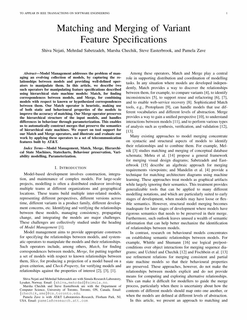
Fig. 1. Simplified variants of the call logger feature.
merging variant feature specifications described as Statechartmodels. Merging combines structural and semantic informa-tion present in the Statechart models and ensures that theirbehavioural properties are preserved. In our work, we separateidentification of model relationships from model integrationby providing independent Match and Merge operators. OurMatch operator includes heuristics for finding terminological,structural, and semantic similarities between models. OurMerge operator parameterizes variabilities between the inputmodels so that their behavioural properties are guaranteed tobe preserved in their merge. We report on tool support for ourMatch and Merge operators, and illustrate and evaluate ourwork by applying these operators to a set of telecommunica-tion features built by AT&T.
A. Motivating ExampleDomain. We motivate our work with a scenario for maintain-ing variant feature specifications at AT&T. These executablespecifications are modules within the Distributed Feature Com-position (DFC) architecture [17], [18], and form part of aconsumer voice-over-IP service [19]. The features are specifiedas Statecharts.
One feature of the voice-over-IP service is “call logging”,which makes an external record of the disposition of a callallowing customers to later view information on calls theyplaced or received. At an abstract level, the feature works asfollows: It first tries to setup a connection between the callerand the callee. If for any reason (e.g., the caller hanging upor the callee not responding), a connection is not established,a failure is logged; otherwise, when the call is completed,information about the call is logged.
Initially, the functionality was designed only for basic phonecalls, for which logging is limited to the direction of a call,
P1 After a connection is set up, a successful call will be loggedif the subscriber or the participant sends Accept
P2 After a connection is set up, a voicemail will be loggedif the call is redirected to the voicemail service
Fig. 2. Sample behavioural properties of the models in Figure 1: P1represents an overlapping behaviour, and P2 – a non-overlapping one.
the address location where a call is answered, success orfailure of the call, and the duration if it succeeds. Later,a variant of this feature was developed for customers whosubscribe to the voicemail service. Incoming calls for thesecustomers may be redirected to a voicemail resource, andhence, the log information should include the voicemail statusas well. Figure 1 shows simplified views of the basic andvoicemail variants of this feature. To avoid clutter, we combinetransitions that have the same source and target states usingthe disjunction (OR) operator.
In the DFC architecture, telecom features may come inseveral variants to accommodate different customers’ needs.The development of these variants is often distributed acrosstime and over different teams of people, resulting in theconstruction of independent but overlapping models for eachfeature. For example, consider the two properties described inFigure 2. Property P1 holds in both variants shown in Figure 1because both can log a successful call: P1 holds via the pathfrom s4 to s6 in the basic variant, and via the path from t4 tot6 in voicemail. This property represents a potential overlapbetween the behaviours of these variants. In contrast, propertyP2 only holds in voicemail (via the path from t4 to t8) butnot in basic. This property illustrates a behavioural variationbetween the variants shown in Figure 1.
Goal. To reduce the high costs associated with verifying
TO APPEAR IN IEEE TRANSACTIONS ON SOFTWARE ENGINEERING 3
and maintaining independent models, we need to identifycorrespondences between variant models so that developerscan obtain a single unified model.
B. Contributions of this article
Applications of Match and Merge arise in a number ofdifferent contexts, one of which is illustrated by our motivatingexample. Implementing Match and Merge involves answeringseveral questions. Particularly, what criteria should we use foridentifying correspondences between different models? Howcan we quantify these criteria? How can we construct a mergegiven a set of models and their correspondences? How canwe distinguish between shared and non-shared parts of theinput models in their merge? What properties of the inputmodels should be preserved by their merge? In this article, weaddress these questions for models expressed as Statecharts.This article extends and refines an earlier version of this workwhich appeared in [20], making the following contributions:• A description of a versatile Match operator for hierarchi-
cal state machines. Our Match operator uses a range ofheuristics including typographic and linguistic similaritiesbetween the vocabularies of different models, structuralsimilarities between the hierarchical nesting of modelelements, and semantic similarities between models basedon a quantitative notion of behavioural bisimulation. Weapply our Match operator to a set of telecom feature spec-ifications developed by AT&T. Our evaluation indicatesthat the approach is effective for finding correspondencesbetween real-world models.
• A description of a Merge operator for Statechart mod-els. We provide a procedure for constructing behaviour-preserving merges that also respect the hierarchical struc-turing and parallelism of the input models. We use thisMerge operator for combining variant telecom featuresfrom AT&T based on the relationships computed by ourMatch operator between the features.
• Tool support for our Match and Mergeoperators. Our tool, named TReMer+(http://se.cs.toronto.edu/index.php/TReMer) [21], enablesestablishing relationships between models – identifiedmanually or based on results of our Match operator –and computes the result of Merge for each identifiedrelationship.
The rest of this article is organized as follows. Section IIprovides an overview of our Match and Merge operators. Sec-tion III outlines our assumptions and fixes notation. Section IVintroduces our Match operator, and Section V – our Mergeoperator. Section VI describes tool support for the two oper-ators. Section VII presents an evaluation of effectiveness forthe Match operator, and Section VIII assesses the soundnessof the Merge operator. Section IX compares our contributionswith related work and discusses the results presented in thisarticle. Finally, Section X concludes the article.
II. OVERVIEW OF OUR APPROACH
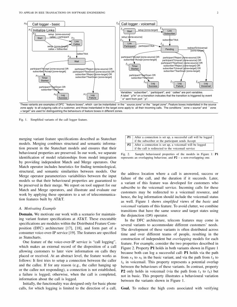
Figure 3 provides an overview of our framework for in-tegrating variant feature specifications. The framework has
Fig. 3. A framework for integrating variant feature specifications.
two main steps. In the first step, a Match operator is usedto find relationships between the input models. In the secondstep, an appropriate Merge operator is used to combine themodels with respect to the relationships computed by Match.This framework enables the explicit distinction between theidentification of model relationships and model integration –the Match and Merge operators are independent, but they areused synergistically to allow us to hypothesize alternative waysof combining models, and to compute the result of merge foreach alternative.
Our ultimate goal is to provide automated tool supportfor the framework in Figure 3. Among these two operators,Match has a heuristic nature. Since models are developedindependently, we can never be entirely sure about how thesemodels are related. At best, we can find heuristics that canimitate the reasoning of a domain expert. In our work, we usetwo types of heuristics: static and behavioural. Static heuristicsuse structural and textual attributes, such as element names,for measuring similarities. For the models in Figure 1, staticheuristics would suggest a number of good correspondences,e.g., the pairs (s6, t6), and (s7, t7); however, these heuristicswould miss several others, including (s3, t3), (s3, t2) and(s4, t4). These pairs are likely to correspond not because theyhave similar static characteristics, but because they exhibitsimilar dynamic behaviours. Our behavioural heuristic can findthese pairs.
To obtain a satisfactory correspondence relation, we use acombination of static and behavioural heuristics. Our Matchoperator produces a correspondence relation between statesin the two models. For the models in Figure 1, it may yieldthe correspondence relation shown in Figure 8(b). Becausethe approach is heuristic, the relation must be reviewed by adomain expert and adjusted by adding any missing correspon-dences and removing any spurious ones. In our example, thefinal correspondence relation approved by a domain expert isshown in Figure 8(d).
Unlike matching, merging is not heuristic, and in situationswhere the purpose of merge is clear, this operator is entirelyautomatable. Given a pair of models and a correspondencerelation between them, our Merge operator automatically pro-duces a merge that:
1) preserves the behavioural properties of the input models.Figure 10 shows the merge of the models of Figure 1with respect to the relation in Figure 8(d). This mergeis behaviour-preserving. That is, any behaviour of theinput models is preserved in the merge model (either
TO APPEAR IN IEEE TRANSACTIONS ON SOFTWARE ENGINEERING 4
through shared or non-shared behaviours). For example,the property P1 in Figure 2 that shows an overlappingbehaviour between the models in Figure 1 is preservedin the merge as a shared behaviour (denoted by the pathfrom state (s4, t4) to (s6, t6)).
2) distinguishes between shared and non-shared behavioursof the input models by attaching appropriate guardconditions to non-shared transitions. In the merge, non-shared transitions are guarded by boldface conditionsrepresenting the models they originate from. For exam-ple, the property P2 in Figure 2 which holds over thevoicemail variant but not over the basic, is representedas a parameterized behaviour in the merge (denoted bythe transition from (s4, t4) to t8), and is preserved onlywhen its guard holds.
3) respects the hierarchical structure and parallelism of theinput models, providing users with a merge that has thesame conceptual structure as the input models.
III. ASSUMPTIONS AND BACKGROUND
The Statechart language [22] is a common notation for de-scribing hierarchical state machines and is a de-facto standardfor specifying intra-object behaviours of software systems.Below, the syntax of this language is formalized [23].
Definition 1 (Statecharts): A Statecharts model is a tuple(S, s, <h, E, V,R), where S is a finite set of states; s ∈ S is aninitial state; <h is an AND-OR tree defining the state hierarchytree (or hierarchy tree, for short); E is a finite set of events; Vis a finite set of variables; and R is a finite set of transitions,each of which is of the form 〈s, e, c, α, s′, prty〉, where s, s′ ∈S are the transition’s source and target, respectively, e ∈ E isthe triggering event, c is an optional predicate over V , α isa sequence of zero or more actions that generate events andassign values to variables in V , and prty is a number denotingthe transition’s priority.
We write a transition 〈s, e, c, α, s′, prty〉 as se[c]/α−→ prty s
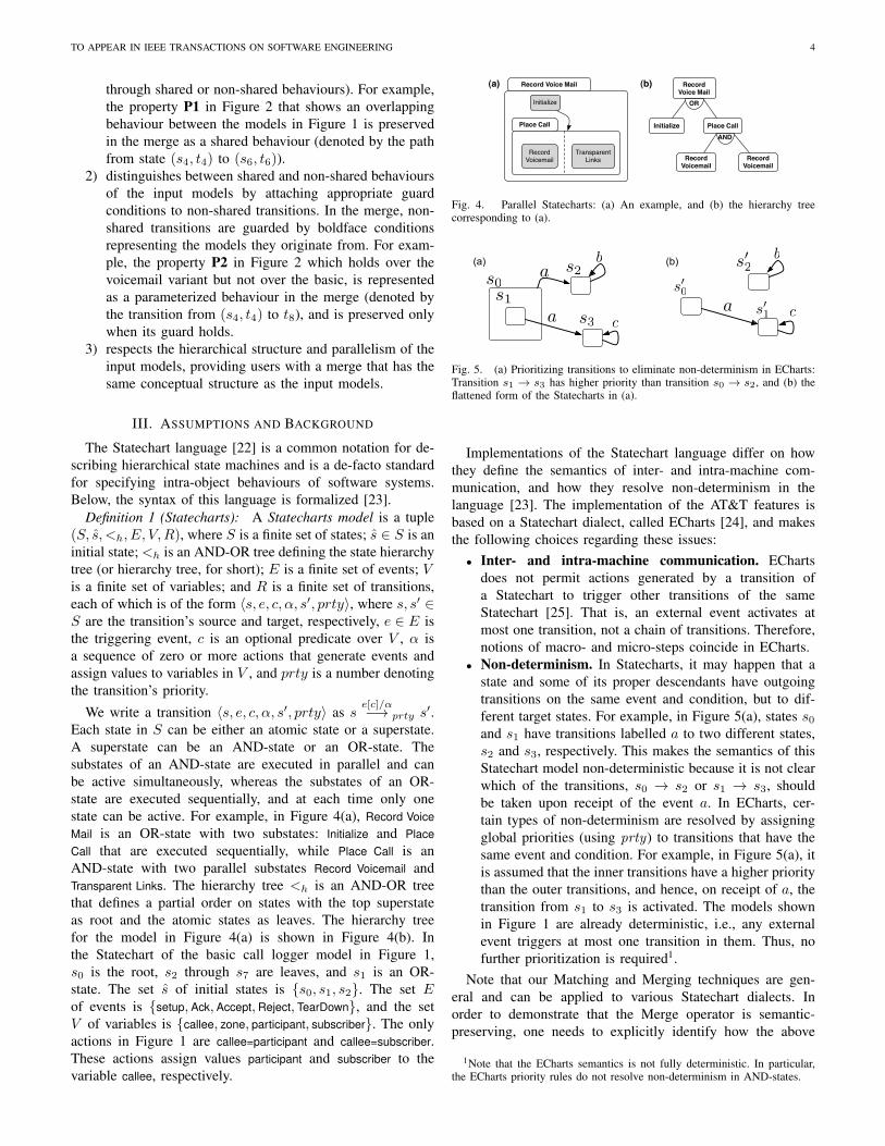
′.Each state in S can be either an atomic state or a superstate.A superstate can be an AND-state or an OR-state. Thesubstates of an AND-state are executed in parallel and canbe active simultaneously, whereas the substates of an OR-state are executed sequentially, and at each time only onestate can be active. For example, in Figure 4(a), Record VoiceMail is an OR-state with two substates: Initialize and PlaceCall that are executed sequentially, while Place Call is anAND-state with two parallel substates Record Voicemail andTransparent Links. The hierarchy tree <h is an AND-OR treethat defines a partial order on states with the top superstateas root and the atomic states as leaves. The hierarchy treefor the model in Figure 4(a) is shown in Figure 4(b). Inthe Statechart of the basic call logger model in Figure 1,s0 is the root, s2 through s7 are leaves, and s1 is an OR-state. The set s of initial states is {s0, s1, s2}. The set Eof events is {setup, Ack, Accept,Reject, TearDown}, and the setV of variables is {callee, zone, participant, subscriber}. The onlyactions in Figure 1 are callee=participant and callee=subscriber.These actions assign values participant and subscriber to thevariable callee, respectively.
Initialize
Record Voicemail
Transparent Links
Record Voice Mail
Place Call
(a) Record Voice Mail
(b)
Initialize Place Call
OR
RecordVoicemail
RecordVoicemail
AND
Fig. 4. Parallel Statecharts: (a) An example, and (b) the hierarchy treecorresponding to (a).
s1
a
s0a
a
b
c
s′0
cs′1
(a) (b)s2
s3
bs′2
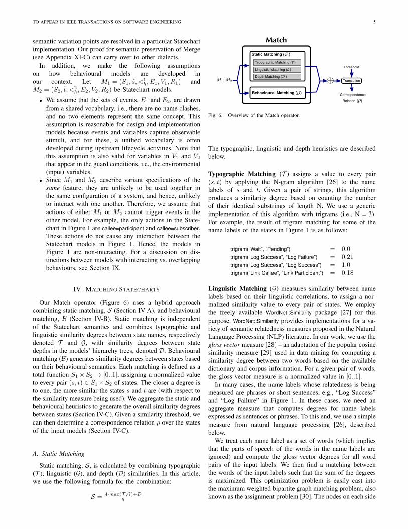
Fig. 5. (a) Prioritizing transitions to eliminate non-determinism in ECharts:Transition s1 → s3 has higher priority than transition s0 → s2, and (b) theflattened form of the Statecharts in (a).
Implementations of the Statechart language differ on howthey define the semantics of inter- and intra-machine com-munication, and how they resolve non-determinism in thelanguage [23]. The implementation of the AT&T features isbased on a Statechart dialect, called ECharts [24], and makesthe following choices regarding these issues:• Inter- and intra-machine communication. ECharts
does not permit actions generated by a transition ofa Statechart to trigger other transitions of the sameStatechart [25]. That is, an external event activates atmost one transition, not a chain of transitions. Therefore,notions of macro- and micro-steps coincide in ECharts.
• Non-determinism. In Statecharts, it may happen that astate and some of its proper descendants have outgoingtransitions on the same event and condition, but to dif-ferent target states. For example, in Figure 5(a), states s0and s1 have transitions labelled a to two different states,s2 and s3, respectively. This makes the semantics of thisStatechart model non-deterministic because it is not clearwhich of the transitions, s0 → s2 or s1 → s3, shouldbe taken upon receipt of the event a. In ECharts, cer-tain types of non-determinism are resolved by assigningglobal priorities (using prty) to transitions that have thesame event and condition. For example, in Figure 5(a), itis assumed that the inner transitions have a higher prioritythan the outer transitions, and hence, on receipt of a, thetransition from s1 to s3 is activated. The models shownin Figure 1 are already deterministic, i.e., any externalevent triggers at most one transition in them. Thus, nofurther prioritization is required1.
Note that our Matching and Merging techniques are gen-eral and can be applied to various Statechart dialects. Inorder to demonstrate that the Merge operator is semantic-preserving, one needs to explicitly identify how the above
1Note that the ECharts semantics is not fully deterministic. In particular,the ECharts priority rules do not resolve non-determinism in AND-states.
TO APPEAR IN IEEE TRANSACTIONS ON SOFTWARE ENGINEERING 5
semantic variation points are resolved in a particular Statechartimplementation. Our proof for semantic preservation of Merge(see Appendix XI-C) can carry over to other dialects.
In addition, we make the following assumptionson how behavioural models are developed inour context. Let M1 = (S1, s, <
1h, E1, V1, R1) and
M2 = (S2, t, <2h, E2, V2, R2) be Statechart models.
• We assume that the sets of events, E1 and E2, are drawnfrom a shared vocabulary, i.e., there are no name clashes,and no two elements represent the same concept. Thisassumption is reasonable for design and implementationmodels because events and variables capture observablestimuli, and for these, a unified vocabulary is oftendeveloped during upstream lifecycle activities. Note thatthis assumption is also valid for variables in V1 and V2that appear in the guard conditions, i.e., the environmental(input) variables.
• Since M1 and M2 describe variant specifications of thesame feature, they are unlikely to be used together inthe same configuration of a system, and hence, unlikelyto interact with one another. Therefore, we assume thatactions of either M1 or M2 cannot trigger events in theother model. For example, the only actions in the State-chart in Figure 1 are callee=participant and callee=subscriber.These actions do not cause any interaction between theStatechart models in Figure 1. Hence, the models inFigure 1 are non-interacting. For a discussion on dis-tinctions between models with interacting vs. overlappingbehaviours, see Section IX.
IV. MATCHING STATECHARTS
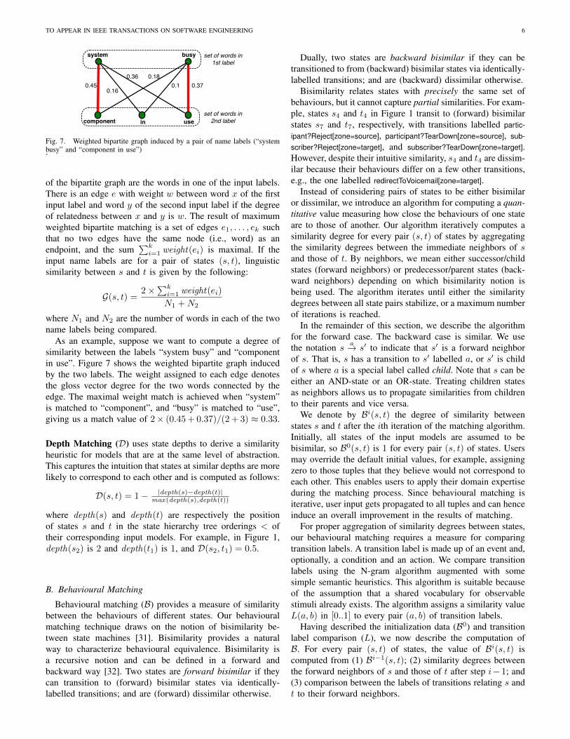
Our Match operator (Figure 6) uses a hybrid approachcombining static matching, S (Section IV-A), and behaviouralmatching, B (Section IV-B). Static matching is independentof the Statechart semantics and combines typographic andlinguistic similarity degrees between state names, respectivelydenoted T and G, with similarity degrees between statedepths in the models’ hierarchy trees, denoted D. Behaviouralmatching (B) generates similarity degrees between states basedon their behavioural semantics. Each matching is defined as atotal function S1 × S2 → [0..1], assigning a normalized valueto every pair (s, t) ∈ S1×S2 of states. The closer a degree isto one, the more similar the states s and t are (with respect tothe similarity measure being used). We aggregate the static andbehavioural heuristics to generate the overall similarity degreesbetween states (Section IV-C). Given a similarity threshold, wecan then determine a correspondence relation ρ over the statesof the input models (Section IV-C).
A. Static Matching
Static matching, S , is calculated by combining typographic(T ), linguistic (G), and depth (D) similarities. In this article,we use the following formula for the combination:
S = 4·max(T ,G)+D5
CorrespondenceRelation ( )ρ
+ Translation
Threshold
M1,M2
Static Matching ( )
Behavioural Matching ( )
S
B
Typographic Matching ( )
Linguistic Matching ( )
Depth Matching ( )
TG
D
Match
Fig. 6. Overview of the Match operator.
The typographic, linguistic and depth heuristics are describedbelow.
Typographic Matching (T ) assigns a value to every pair(s, t) by applying the N-gram algorithm [26] to the namelabels of s and t. Given a pair of strings, this algorithmproduces a similarity degree based on counting the numberof their identical substrings of length N. We use a genericimplementation of this algorithm with trigrams (i.e., N = 3).For example, the result of trigram matching for some of thename labels of the states in Figure 1 is as follows:
trigram(“Wait”, “Pending”) = 0.0trigram(“Log Success”, “Log Failure”) = 0.21trigram(“Log Success”, “Log Success”) = 1.0trigram(“Link Callee”, “Link Participant”) = 0.18
Linguistic Matching (G) measures similarity between namelabels based on their linguistic correlations, to assign a nor-malized similarity value to every pair of states. We employthe freely available WordNet::Similarity package [27] for thispurpose. WordNet::Similarity provides implementations for a va-riety of semantic relatedness measures proposed in the NaturalLanguage Processing (NLP) literature. In our work, we use thegloss vector measure [28] – an adaptation of the popular cosinesimilarity measure [29] used in data mining for computing asimilarity degree between two words based on the availabledictionary and corpus information. For a given pair of words,the gloss vector measure is a normalized value in [0..1].
In many cases, the name labels whose relatedness is beingmeasured are phrases or short sentences, e.g., “Log Success”and “Log Failure” in Figure 1. In these cases, we need anaggregate measure that computes degrees for name labelsexpressed as sentences or phrases. To this end, we use a simplemeasure from natural language processing [26], describedbelow.
We treat each name label as a set of words (which impliesthat the parts of speech of the words in the name labels areignored) and compute the gloss vector degrees for all wordpairs of the input labels. We then find a matching betweenthe words of the input labels such that the sum of the degreesis maximized. This optimization problem is easily cast intothe maximum weighted bipartite graph matching problem, alsoknown as the assignment problem [30]. The nodes on each side
TO APPEAR IN IEEE TRANSACTIONS ON SOFTWARE ENGINEERING 6
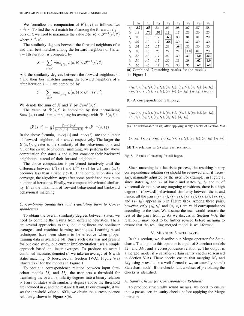
system busy
component in use
0.450.18
0.16
0.360.370.1
set of words in 2nd label
set of words in 1st label
Fig. 7. Weighted bipartite graph induced by a pair of name labels (“systembusy” and “component in use”).
of the bipartite graph are the words in one of the input labels.There is an edge e with weight w between word x of the firstinput label and word y of the second input label if the degreeof relatedness between x and y is w. The result of maximumweighted bipartite matching is a set of edges e1, . . . , ek suchthat no two edges have the same node (i.e., word) as anendpoint, and the sum
∑ki=1 weight(ei) is maximal. If the
input name labels are for a pair of states (s, t), linguisticsimilarity between s and t is given by the following:
G(s, t) =2×∑k
i=1 weight(ei)
N1 +N2
where N1 and N2 are the number of words in each of the twoname labels being compared.
As an example, suppose we want to compute a degree ofsimilarity between the labels “system busy” and “componentin use”. Figure 7 shows the weighted bipartite graph inducedby the two labels. The weight assigned to each edge denotesthe gloss vector degree for the two words connected by theedge. The maximal weight match is achieved when “system”is matched to “component”, and “busy” is matched to “use”,giving us a match value of 2× (0.45 + 0.37)/(2 + 3) ≈ 0.33.
Depth Matching (D) uses state depths to derive a similarityheuristic for models that are at the same level of abstraction.This captures the intuition that states at similar depths are morelikely to correspond to each other and is computed as follows:
D(s, t) = 1− |depth(s)−depth(t)|max(depth(s),depth(t))
where depth(s) and depth(t) are respectively the positionof states s and t in the state hierarchy tree orderings < oftheir corresponding input models. For example, in Figure 1,depth(s2) is 2 and depth(t1) is 1, and D(s2, t1) = 0.5.
B. Behavioural Matching
Behavioural matching (B) provides a measure of similaritybetween the behaviours of different states. Our behaviouralmatching technique draws on the notion of bisimilarity be-tween state machines [31]. Bisimilarity provides a naturalway to characterize behavioural equivalence. Bisimilarity isa recursive notion and can be defined in a forward andbackward way [32]. Two states are forward bisimilar if theycan transition to (forward) bisimilar states via identically-labelled transitions; and are (forward) dissimilar otherwise.
Dually, two states are backward bisimilar if they can betransitioned to from (backward) bisimilar states via identically-labelled transitions; and are (backward) dissimilar otherwise.
Bisimilarity relates states with precisely the same set ofbehaviours, but it cannot capture partial similarities. For exam-ple, states s4 and t4 in Figure 1 transit to (forward) bisimilarstates s7 and t7, respectively, with transitions labelled partic-ipant?Reject[zone=source], participant?TearDown[zone=source], sub-scriber?Reject[zone=target], and subscriber?TearDown[zone=target].However, despite their intuitive similarity, s4 and t4 are dissim-ilar because their behaviours differ on a few other transitions,e.g., the one labelled redirectToVoicemail[zone=target].
Instead of considering pairs of states to be either bisimilaror dissimilar, we introduce an algorithm for computing a quan-titative value measuring how close the behaviours of one stateare to those of another. Our algorithm iteratively computes asimilarity degree for every pair (s, t) of states by aggregatingthe similarity degrees between the immediate neighbors of sand those of t. By neighbors, we mean either successor/childstates (forward neighbors) or predecessor/parent states (back-ward neighbors) depending on which bisimilarity notion isbeing used. The algorithm iterates until either the similaritydegrees between all state pairs stabilize, or a maximum numberof iterations is reached.
In the remainder of this section, we describe the algorithmfor the forward case. The backward case is similar. We usethe notation s
a→ s′ to indicate that s′ is a forward neighborof s. That is, s has a transition to s′ labelled a, or s′ is childof s where a is a special label called child. Note that s can beeither an AND-state or an OR-state. Treating children statesas neighbors allows us to propagate similarities from childrento their parents and vice versa.
We denote by Bi(s, t) the degree of similarity betweenstates s and t after the ith iteration of the matching algorithm.Initially, all states of the input models are assumed to bebisimilar, so B0(s, t) is 1 for every pair (s, t) of states. Usersmay override the default initial values, for example, assigningzero to those tuples that they believe would not correspond toeach other. This enables users to apply their domain expertiseduring the matching process. Since behavioural matching isiterative, user input gets propagated to all tuples and can henceinduce an overall improvement in the results of matching.
For proper aggregation of similarity degrees between states,our behavioural matching requires a measure for comparingtransition labels. A transition label is made up of an event and,optionally, a condition and an action. We compare transitionlabels using the N-gram algorithm augmented with somesimple semantic heuristics. This algorithm is suitable becauseof the assumption that a shared vocabulary for observablestimuli already exists. The algorithm assigns a similarity valueL(a, b) in [0..1] to every pair (a, b) of transition labels.
Having described the initialization data (B0) and transitionlabel comparison (L), we now describe the computation ofB. For every pair (s, t) of states, the value of Bi(s, t) iscomputed from (1) Bi−1(s, t); (2) similarity degrees betweenthe forward neighbors of s and those of t after step i− 1; and(3) comparison between the labels of transitions relating s andt to their forward neighbors.
TO APPEAR IN IEEE TRANSACTIONS ON SOFTWARE ENGINEERING 7
We formalize the computation of Bi(s, t) as follows. Letsa→ s′. To find the best match for s′ among the forward neigh-
bors of t, we need to maximize the value L(a, b)× Bi−1(s′, t′)
where t b→ t′.The similarity degrees between the forward neighbors of s
and their best matches among the forward neighbors of t afteri− 1th iteration is computed by
X =∑s
a→s′max
tb→t′L(a, b)× Bi−1(s′, t′)
And the similarity degrees between the forward neighbors oft and their best matches among the forward neighbors of safter iteration i− 1 are computed by
Y =∑t
a→t′max
sb→s′L(a, b)× Bi−1(s′, t′)
We denote the sum of X and Y by Sumi(s, t).The value of Bi(s, t) is computed by first normalizing
Sumi(s, t) and then computing its average with Bi−1(s, t):
Bi(s, t) = 12
( Sumi(s,t)|succ(s)|+|succ(t)| + B
i−1(s, t))
In the above formula, |succ(s)| and |succ(t)| are the numberof forward neighbors of s and t, respectively. The larger theBi(s, t), greater is the similarity of the behaviours of s andt. For backward behavioural matching, we perform the abovecomputation for states s and t, but consider their backwardneighbours instead of their forward neighbours.
The above computation is performed iteratively until thedifference between Bi(s, t) and Bi−1(s, t) for all pairs (s, t)becomes less than a fixed ε > 0. If the computation does notconverge, the algorithm stops after some predefined maximumnumber of iterations. Finally, we compute behavioural similar-ity, B, as the maximum of forward behavioural and backwardbehavioural matching.
C. Combining Similarities and Translating them to Corre-spondences
To obtain the overall similarity degrees between states, weneed to combine the results from different heuristics. Thereare several approaches to this, including linear and nonlinearaverages, and machine learning techniques. Learning-basedtechniques have been shown to be effective when propertraining data is available [4]. Since such data was not presentfor our case study, our current implementation uses a simpleapproach based on linear averages. To produce an overallcombined measure, denoted C, we take an average of B withstatic matching, S (described in Section IV-A). Figure 8(a)illustrates C for the models in Figure 1.
To obtain a correspondence relation between input Stat-echart models M1 and M2, the user sets a threshold fortranslating the overall similarity degrees into a binary relationρ. Pairs of states with similarity degrees above the thresholdare included in ρ, and the rest are left out. In our example, if weset the threshold value to 60%, we obtain the correspondencerelation ρ shown in Figure 8(b).
s0 s1 s2 s3 s4 s5 s6 s7
t0 .87 .63 .54 .03 .08 .07 .57 .58
t1 .48 .70 .92 .17 .17 .26 .20 .23
t2 .08 .18 .17 .65 .30 .31 .31 .29
t3 .07 .19 .17 .66 .30 .32 .30 .30
t4 .07 .15 .17 .23 .64 .30 .30 .30
t5 .08 .15 .25 .22 .24 1.0 .04 .28
t6 .58 .45 .17 .22 .30 .30 1.0 .63t7 .56 .45 .17 .22 .31 .28 .62 1.0t8 .55 .45 .17 .22 .30 .35 .62 .62
(a) Combined C matching results for the modelsin Figure 1.
(s0, t0), (s2, t1), (s3, t2), (s3, t3), (s4, t4), (s5, t5), (s6, t6),(s7, t7), (s1, t0), (s1, t1), (s6, t7), (s6, t8), (s7, t6), (s7, t8)
(b) A correspondence relation ρ.
(s0, t0), (s2, t1), (s3, t2), (s3, t3), (s4, t4), (s5, t5), (s6, t6),(s7, t7), (s6, t7), (s6, t8), (s7, t6), (s7, t8)
(c) The relationship in (b) after applying sanity checks of Section V-A.
(s0, t0), (s4, t4), (s2, t1), (s5, t5), (s3, t2), (s6, t6), (s3, t3), (s7, t7)
(d) The relations in (c) after user revisions.
Fig. 8. Results of matching for call logger.
Since matching is a heuristic process, the resulting binarycorrespondence relation (ρ) should be reviewed and, if neces-sary, manually adjusted by the user. For example, in Figure 1,since states s6 and s7 of basic and states t6, t7 and t8 ofvoicemail do not have any outgoing transitions, there is a highdegree of (forward) behavioural similarity between them, andhence, all the pairs (s6, t6), (s6, t7), (s6, t8), (s7, t6), (s7, t7),and (s7, t8) appear in ρ in Figure 8(b). Among these pairs,however, only (s6, t6) and (s7, t7) are valid correspondencesaccording to the user. We assume the user would remove therest of the pairs from ρ. As we discuss in Section V-A, therelation ρ may need to be further revised before merging toensure that the resulting merged model is well-formed.
V. MERGING STATECHARTS
In this section, we describe our Merge operator for State-charts. The input to this operator is a pair of Statechart modelsM1 and M2, and a correspondence relation ρ. The output isa merged model if ρ satisfies certain sanity checks (discussedin Section V-A). These checks ensure that merging M1 andM2 using ρ results in a well-formed (i.w., structurally sound)Statechart model. If the checks fail, a subset of ρ violating thechecks is identified.
A. Sanity Checks for Correspondence RelationsTo produce structurally sound merges, we need to ensure
that ρ passes certain sanity checks before applying the Mergeoperator:
TO APPEAR IN IEEE TRANSACTIONS ON SOFTWARE ENGINEERING 8
ss′ t′
t
s
t′t
s0 snsi
t′′
sk
✘s ts0 snsi
✘
t0 tmtj tk
✘
(a) (b)
(c)
· · · · · · · · ·
· · · · · · · · · · · · · · ·
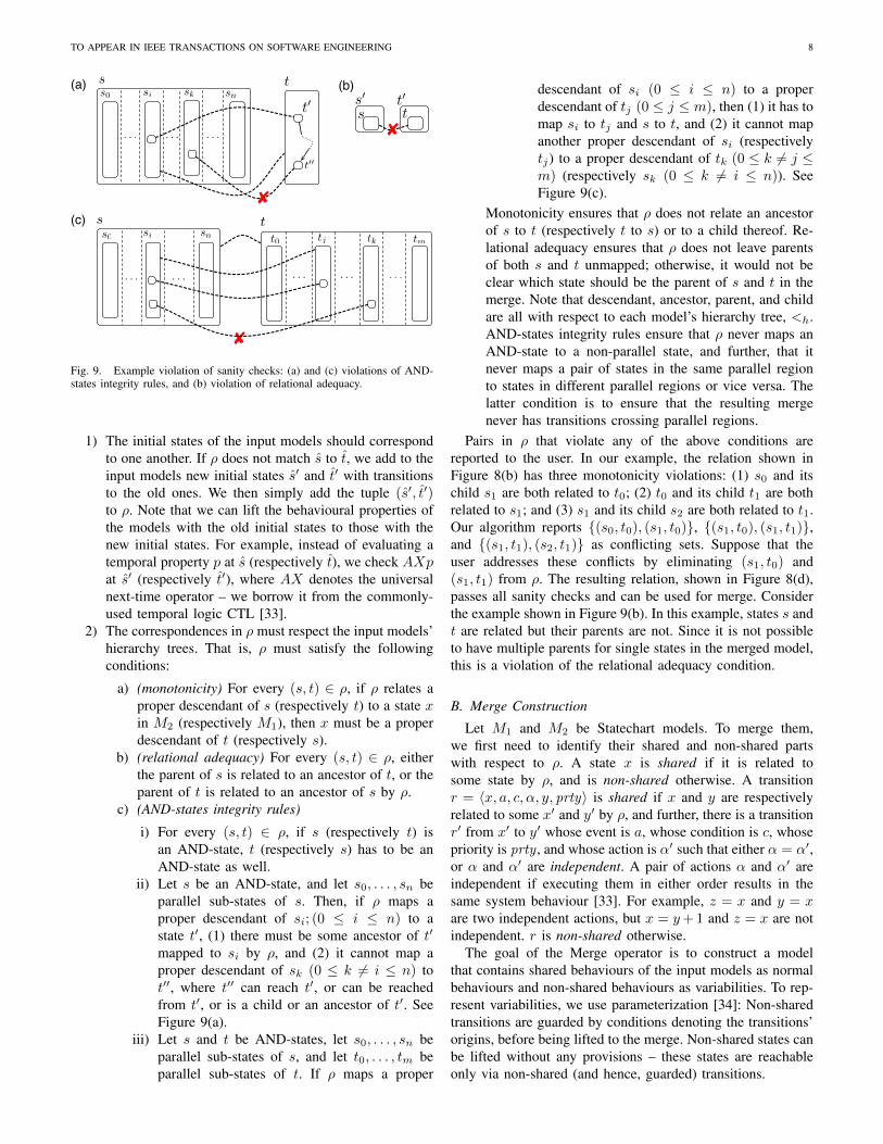
Fig. 9. Example violation of sanity checks: (a) and (c) violations of AND-states integrity rules, and (b) violation of relational adequacy.
1) The initial states of the input models should correspondto one another. If ρ does not match s to t, we add to theinput models new initial states s′ and t′ with transitionsto the old ones. We then simply add the tuple (s′, t′)to ρ. Note that we can lift the behavioural properties ofthe models with the old initial states to those with thenew initial states. For example, instead of evaluating atemporal property p at s (respectively t), we check AXpat s′ (respectively t′), where AX denotes the universalnext-time operator – we borrow it from the commonly-used temporal logic CTL [33].
2) The correspondences in ρ must respect the input models’hierarchy trees. That is, ρ must satisfy the followingconditions:
a) (monotonicity) For every (s, t) ∈ ρ, if ρ relates aproper descendant of s (respectively t) to a state xin M2 (respectively M1), then x must be a properdescendant of t (respectively s).
b) (relational adequacy) For every (s, t) ∈ ρ, eitherthe parent of s is related to an ancestor of t, or theparent of t is related to an ancestor of s by ρ.
c) (AND-states integrity rules)
i) For every (s, t) ∈ ρ, if s (respectively t) isan AND-state, t (respectively s) has to be anAND-state as well.
ii) Let s be an AND-state, and let s0, . . . , sn beparallel sub-states of s. Then, if ρ maps aproper descendant of si; (0 ≤ i ≤ n) to astate t′, (1) there must be some ancestor of t′
mapped to si by ρ, and (2) it cannot map aproper descendant of sk (0 ≤ k 6= i ≤ n) tot′′, where t′′ can reach t′, or can be reachedfrom t′, or is a child or an ancestor of t′. SeeFigure 9(a).
iii) Let s and t be AND-states, let s0, . . . , sn beparallel sub-states of s, and let t0, . . . , tm beparallel sub-states of t. If ρ maps a proper
descendant of si (0 ≤ i ≤ n) to a properdescendant of tj (0 ≤ j ≤ m), then (1) it has tomap si to tj and s to t, and (2) it cannot mapanother proper descendant of si (respectivelytj) to a proper descendant of tk (0 ≤ k 6= j ≤m) (respectively sk (0 ≤ k 6= i ≤ n)). SeeFigure 9(c).
Monotonicity ensures that ρ does not relate an ancestorof s to t (respectively t to s) or to a child thereof. Re-lational adequacy ensures that ρ does not leave parentsof both s and t unmapped; otherwise, it would not beclear which state should be the parent of s and t in themerge. Note that descendant, ancestor, parent, and childare all with respect to each model’s hierarchy tree, <h.AND-states integrity rules ensure that ρ never maps anAND-state to a non-parallel state, and further, that itnever maps a pair of states in the same parallel regionto states in different parallel regions or vice versa. Thelatter condition is to ensure that the resulting mergenever has transitions crossing parallel regions.
Pairs in ρ that violate any of the above conditions arereported to the user. In our example, the relation shown inFigure 8(b) has three monotonicity violations: (1) s0 and itschild s1 are both related to t0; (2) t0 and its child t1 are bothrelated to s1; and (3) s1 and its child s2 are both related to t1.Our algorithm reports {(s0, t0), (s1, t0)}, {(s1, t0), (s1, t1)},and {(s1, t1), (s2, t1)} as conflicting sets. Suppose that theuser addresses these conflicts by eliminating (s1, t0) and(s1, t1) from ρ. The resulting relation, shown in Figure 8(d),passes all sanity checks and can be used for merge. Considerthe example shown in Figure 9(b). In this example, states s andt are related but their parents are not. Since it is not possibleto have multiple parents for single states in the merged model,this is a violation of the relational adequacy condition.
B. Merge Construction
Let M1 and M2 be Statechart models. To merge them,we first need to identify their shared and non-shared partswith respect to ρ. A state x is shared if it is related tosome state by ρ, and is non-shared otherwise. A transitionr = 〈x, a, c, α, y, prty〉 is shared if x and y are respectivelyrelated to some x′ and y′ by ρ, and further, there is a transitionr′ from x′ to y′ whose event is a, whose condition is c, whosepriority is prty , and whose action is α′ such that either α = α′,or α and α′ are independent. A pair of actions α and α′ areindependent if executing them in either order results in thesame system behaviour [33]. For example, z = x and y = xare two independent actions, but x = y+ 1 and z = x are notindependent. r is non-shared otherwise.
The goal of the Merge operator is to construct a modelthat contains shared behaviours of the input models as normalbehaviours and non-shared behaviours as variabilities. To rep-resent variabilities, we use parameterization [34]: Non-sharedtransitions are guarded by conditions denoting the transitions’origins, before being lifted to the merge. Non-shared states canbe lifted without any provisions – these states are reachableonly via non-shared (and hence, guarded) transitions.
TO APPEAR IN IEEE TRANSACTIONS ON SOFTWARE ENGINEERING 9
(Link Callee, Link Subscriber)
(Link Callee, Link Participant)
(Wait, Pending)
(Timer Started, Timer Started)
(Log Failure, Log Failure)
(Log Success, Log Success)
setup [zone =target]/callee = subscriber
setup [zone=source] /callee=participant
participant?Ack [ID=voicemail]
subscriber?Ack[ID=voicemail]
redirectToVoicemail[zone=target,ID=voicemail]
participant?Reject [zone=source] ORparticipant?Unavail [zone=source, ID=voicemail]OR
participant?TearDown [zone=source] ORsubscriber?Reject [zone=target] OR
subscriber?Unavail [in target-zone, ID=voicemail] ORsubscriber?TearDown [zone=target]
participant?TearDown ORsubscriber?TearDown
participant?Accept [zone=source] ORsubscriber?Accept [zone=target]
Log Voicemail
(s0, t0)
callee?Ack[ID=basic]
callee?Ack[ ID=basic]
Call logger - (basic, voicemail)
(Start, Start)
Initialize Linkss1
(s2, t1)(s3, t2)
(s3, t3)
(s4, t4)
(s5, t5)
(s6, t6) (s7, t7) t8
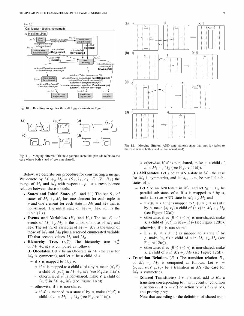
Fig. 10. Resulting merge for the call logger variants in Figure 1.
tss� t�
(s, t)(s�, t�)
=⇒ts
s�(s, t)
=⇒ s�
ss� t� (s�, t�)
=⇒s s
s� =⇒ss�
(a) (b)
(c) (d)
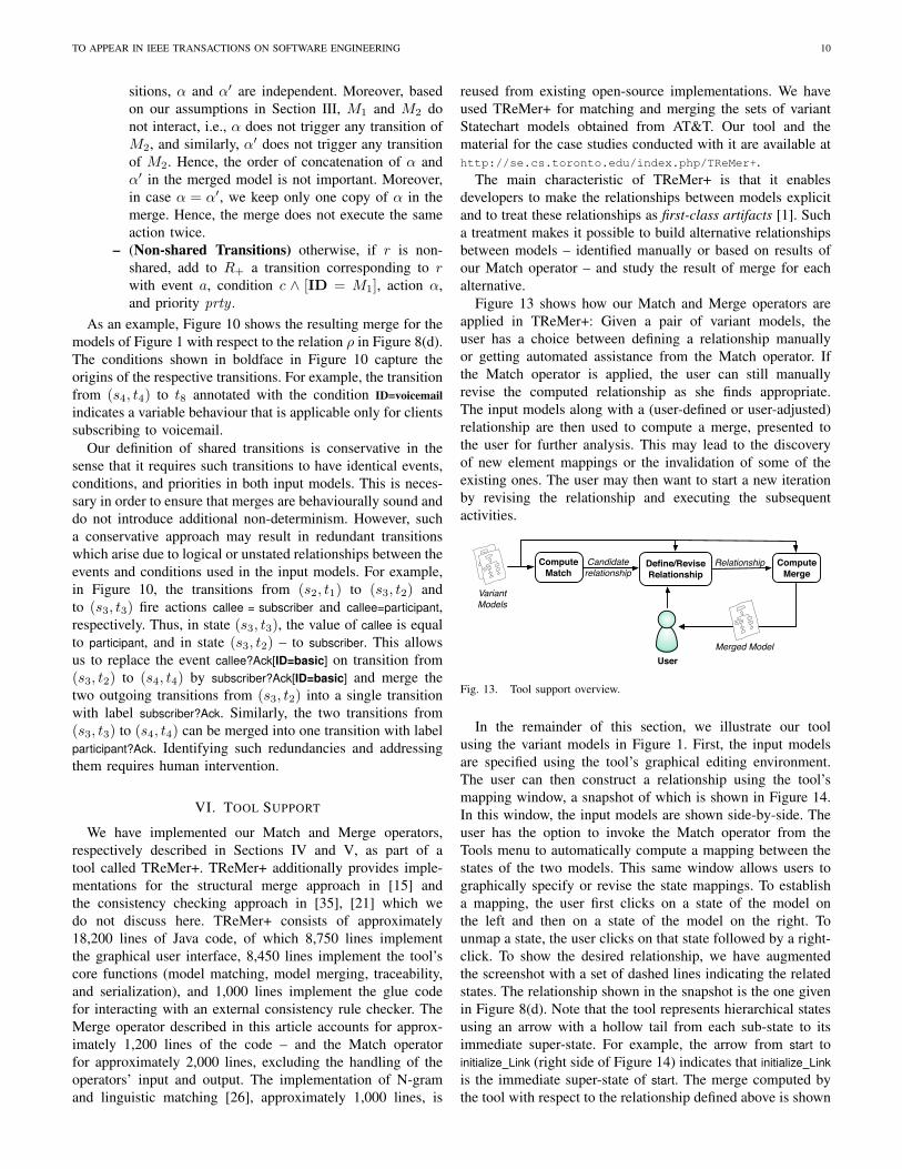
Fig. 11. Merging different OR-state patterns (note that part (d) refers to thecase where both s and s′ are non-shared).
Below, we describe our procedure for constructing a merge.We denote by M1 +ρ M2 = (S+, s+, <
+h , E+, V+, R+) the
merge of M1 and M2 with respect to ρ – a correspondencerelation between these models.• States and Initial State. (S+ and s+) The set S+ of
states of M1 +ρ M2 has one element for each tuple inρ and one element for each state in M1 and M2 that isnon-shared. The initial state of M1 +ρ M2, s+, is thetuple (s, t).
• Events and Variables. (E+ and V+) The set E+ ofevents of M1 +ρ M2 is the union of those of M1 andM2. The set V+ of variables of M1+ρM2 is the union ofthose of M1 and M2 plus a reserved enumerated variableID that accepts values M1 and M2.
• Hierarchy Tree. (<+h ) The hierarchy tree <+
h
of M1 +ρM2 is computed as follows:(I) OR-states. Let s be an OR-state in M1 (the case forM2 is symmetric), and let s′ be a child of s.
– if s is mapped to t by ρ,∗ if s′ is mapped to a child t′ of t by ρ, make (s′, t′)
a child of (s, t) in M1 +ρM2 (see Figure 11(a)).∗ otherwise, if s′ is non-shared, make s′ a child of
(s, t) in M1 +ρM2 (see Figure 11(b)).– otherwise, if s is non-shared∗ if s′ is mapped to a state t′ by ρ, make (s′, t′) a
child of s in M1 +ρM2 (see Figure 11(c)).
s tsi tj
=⇒
(s, t)
(si, tj)
stsi
=⇒
(s, t)si
ssi
=⇒
st′(si, t
′)
ssi
=⇒
ssi
(b)
(a)
(c)
(d)
· · · · · · · · · · · · · · ·· · ·
· · · · · · · · · · · · · · ·
· · · · · · · · · · · ·
· · · · · · · · · · · ·
Fig. 12. Merging different AND-state patterns (note that part (d) refers tothe case where both s and s′ are non-shared).
∗ otherwise, if s′ is non-shared, make s′ a child ofs in M1 +ρM2 (see Figure 11(d)).
(II) AND-states. Let s be an AND-state in M1 (the casefor M2 is symmetric), and let s0, . . . sn be parallel sub-states of s.
– Let t be an AND-state in M2, and let t0, . . . tm beparallel sub-states of t. If s is mapped to t by ρ,make (s, t) an AND-state in M1 +ρM2 and∗ if si(0 ≤ i ≤ n) is mapped to tj (0 ≤ j ≤ m) of t
by ρ, make (si, tj) a child of (s, t) in M1 +ρM2
(see Figure 12(a)).∗ otherwise, if si (0 ≤ i ≤ n) is non-shared, makesi a child of (s, t) in M1+ρM2 (see Figure 12(b)).
– otherwise, if s is non-shared∗ if si (0 ≤ i ≤ n) is mapped to a state t′ byρ, make (si, t
′) a child of s in M1 +ρ M2 (seeFigure 12(c)).
∗ otherwise, if si (0 ≤ i ≤ n) is non-shared, makesi a child of s in M1 +ρM2 (see Figure 12(d)).
• Transition Relation. (R+) The transition relation R+
of M1 +ρ M2 is computed as follows. Let r =〈s, a, c, α, s′, prty〉 be a transition in M1 (the case forM2 is symmetric).
– (Shared Transitions) if r is shared, add to R+ atransition corresponding to r with event a, conditionc, action α (if α = α′) or action α;α′ (if α 6= α′),and priority prty .Note that according to the definition of shared tran-
TO APPEAR IN IEEE TRANSACTIONS ON SOFTWARE ENGINEERING 10
sitions, α and α′ are independent. Moreover, basedon our assumptions in Section III, M1 and M2 donot interact, i.e., α does not trigger any transition ofM2, and similarly, α′ does not trigger any transitionof M2. Hence, the order of concatenation of α andα′ in the merged model is not important. Moreover,in case α = α′, we keep only one copy of α in themerge. Hence, the merge does not execute the sameaction twice.
– (Non-shared Transitions) otherwise, if r is non-shared, add to R+ a transition corresponding to rwith event a, condition c ∧ [ID = M1], action α,and priority prty .
As an example, Figure 10 shows the resulting merge for themodels of Figure 1 with respect to the relation ρ in Figure 8(d).The conditions shown in boldface in Figure 10 capture theorigins of the respective transitions. For example, the transitionfrom (s4, t4) to t8 annotated with the condition ID=voicemailindicates a variable behaviour that is applicable only for clientssubscribing to voicemail.
Our definition of shared transitions is conservative in thesense that it requires such transitions to have identical events,conditions, and priorities in both input models. This is neces-sary in order to ensure that merges are behaviourally sound anddo not introduce additional non-determinism. However, sucha conservative approach may result in redundant transitionswhich arise due to logical or unstated relationships between theevents and conditions used in the input models. For example,in Figure 10, the transitions from (s2, t1) to (s3, t2) andto (s3, t3) fire actions callee = subscriber and callee=participant,respectively. Thus, in state (s3, t3), the value of callee is equalto participant, and in state (s3, t2) – to subscriber. This allowsus to replace the event callee?Ack[ID=basic] on transition from(s3, t2) to (s4, t4) by subscriber?Ack[ID=basic] and merge thetwo outgoing transitions from (s3, t2) into a single transitionwith label subscriber?Ack. Similarly, the two transitions from(s3, t3) to (s4, t4) can be merged into one transition with labelparticipant?Ack. Identifying such redundancies and addressingthem requires human intervention.
VI. TOOL SUPPORT
We have implemented our Match and Merge operators,respectively described in Sections IV and V, as part of atool called TReMer+. TReMer+ additionally provides imple-mentations for the structural merge approach in [15] andthe consistency checking approach in [35], [21] which wedo not discuss here. TReMer+ consists of approximately18,200 lines of Java code, of which 8,750 lines implementthe graphical user interface, 8,450 lines implement the tool’score functions (model matching, model merging, traceability,and serialization), and 1,000 lines implement the glue codefor interacting with an external consistency rule checker. TheMerge operator described in this article accounts for approx-imately 1,200 lines of the code – and the Match operatorfor approximately 2,000 lines, excluding the handling of theoperators’ input and output. The implementation of N-gramand linguistic matching [26], approximately 1,000 lines, is
reused from existing open-source implementations. We haveused TReMer+ for matching and merging the sets of variantStatechart models obtained from AT&T. Our tool and thematerial for the case studies conducted with it are available athttp://se.cs.toronto.edu/index.php/TReMer+.
The main characteristic of TReMer+ is that it enablesdevelopers to make the relationships between models explicitand to treat these relationships as first-class artifacts [1]. Sucha treatment makes it possible to build alternative relationshipsbetween models – identified manually or based on results ofour Match operator – and study the result of merge for eachalternative.
Figure 13 shows how our Match and Merge operators areapplied in TReMer+: Given a pair of variant models, theuser has a choice between defining a relationship manuallyor getting automated assistance from the Match operator. Ifthe Match operator is applied, the user can still manuallyrevise the computed relationship as she finds appropriate.The input models along with a (user-defined or user-adjusted)relationship are then used to compute a merge, presented tothe user for further analysis. This may lead to the discoveryof new element mappings or the invalidation of some of theexisting ones. The user may then want to start a new iterationby revising the relationship and executing the subsequentactivities.
Define/Revise Relationship
ComputeMerge
Relationship
Merged Model
Variant Models
User
Compute Match
Candidaterelationship
Fig. 13. Tool support overview.
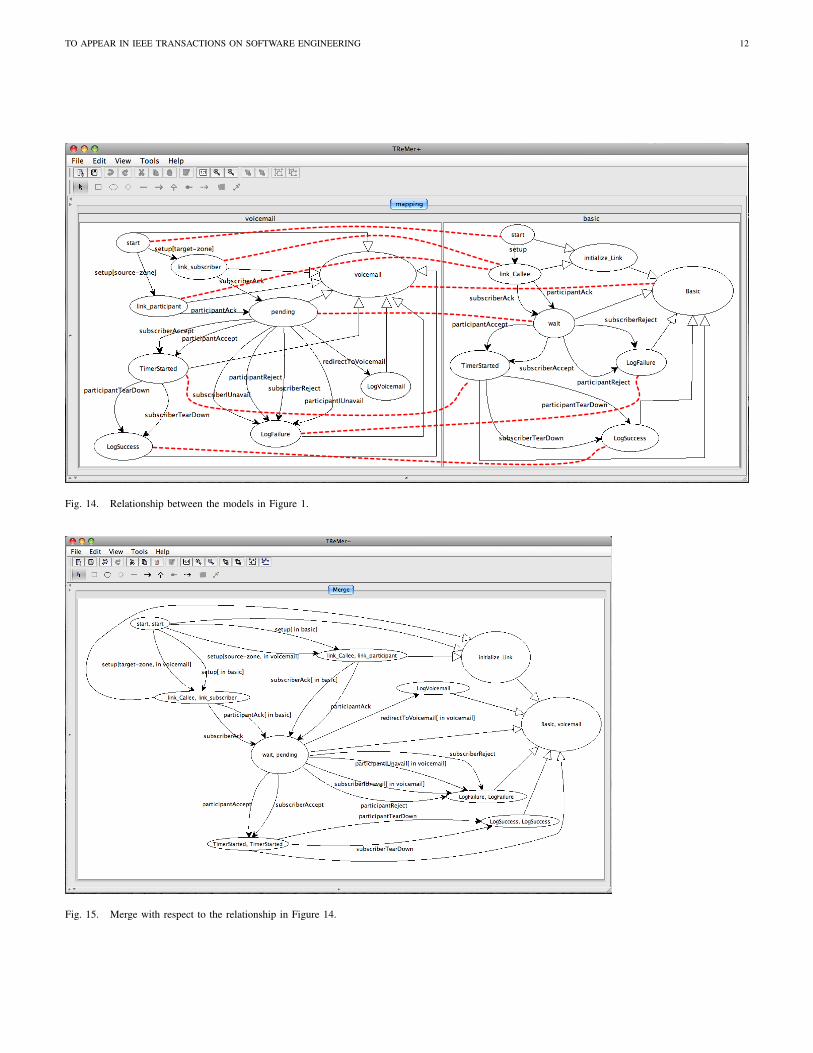
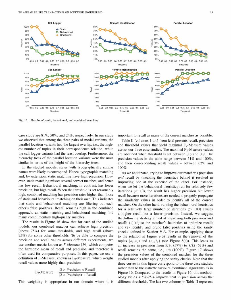
In the remainder of this section, we illustrate our toolusing the variant models in Figure 1. First, the input modelsare specified using the tool’s graphical editing environment.The user can then construct a relationship using the tool’smapping window, a snapshot of which is shown in Figure 14.In this window, the input models are shown side-by-side. Theuser has the option to invoke the Match operator from theTools menu to automatically compute a mapping between thestates of the two models. This same window allows users tographically specify or revise the state mappings. To establisha mapping, the user first clicks on a state of the model onthe left and then on a state of the model on the right. Tounmap a state, the user clicks on that state followed by a right-click. To show the desired relationship, we have augmentedthe screenshot with a set of dashed lines indicating the relatedstates. The relationship shown in the snapshot is the one givenin Figure 8(d). Note that the tool represents hierarchical statesusing an arrow with a hollow tail from each sub-state to itsimmediate super-state. For example, the arrow from start toinitialize Link (right side of Figure 14) indicates that initialize Linkis the immediate super-state of start. The merge computed bythe tool with respect to the relationship defined above is shown
TO APPEAR IN IEEE TRANSACTIONS ON SOFTWARE ENGINEERING 11
in Figure 15. As seen from the figure, non-shared behavioursare guarded by conditions denoting the input model exhibitingthose behaviours.
VII. PROPERTIES OF MATCH
Our approach to matching is valuable if it offers a quick wayto identify appropriate matches with reasonable accuracy, inparticular in situations where matches are hard to find by hand,for example, where the models are complex, or the developersare less familiar with them. Here, we present some steps toevaluate our Match operator. First, we discuss its complexityto show that it scales, and then we assess this operator bymeasuring the accuracy of the relationships it produces, whencompared to the assessment of a human expert.
A. Complexity of Match
Let n1 and n2 be the number of states in the inputmodels, and let m1 and m2 be the number of transitions inthese models. The space and time complexities of computingtypographic and linguistic similarity scores between individualpairs of name labels are negligible and bounded by a constant,i.e., the largest value of similarity scores of the state names.Note that since the set of states names is finite and determined,we can compute such a bound. The space complexity ofMatch is then the storage needed for keeping a state similaritymatrix and a label similarity matrix (L in Section IV-B) and isO(n1×n2+m1×m2). The time complexity of static matchingis O(n1×n2) and of behavioural matching – O(c×m1×m2),where c is the maximum allowed number of iterations for thebehavioural matching algorithm.
B. Evaluation of Match
As with all heuristic matching techniques, the results of ourMatch operator should be reviewed and adjusted by users toobtain a desired correspondence relation. In this sense, a goodway to evaluate a matcher is by considering the number ofadjustments users need to make to the results it produces. Amatcher is effective if it neither produces too many incorrectmatches (false positives) nor misses too many correct matches(false negatives).
We use two well-known information retrieval metrics [36],namely, precision, and recall, to capture this intuition. Preci-sion measures quality (i.e., a low number of false positives)and is the ratio of correct matches found to the total number ofmatches found. Recall measures coverage (i.e., a low numberof false negatives) and is the ratio of the correct matches foundto the total number of all correct matches. For example, ifour matcher produces the relationship in Figure 8(b) and thedesired relation is as shown in Figure 8(d), the precision andrecall are 8/14 (57%) and 8/8 (100%), respectively.
A good matching technique should produce high precisionand high recall. However, these two metrics tend to beinversely related: improvements in recall come at the costof reducing precision and vice versa. In many circumstances,either precision or recall is more important than the other.For example, a web searcher would like every result on the
TABLE INUMBER OF STATES AND TRANSITIONS OF THE STUDIED VARIANT
MODELS.
Feature Variant I Variant II All Correct# states # transitions # states # transitions Matches
Call Logger 18 40 21 63 11Remote Identification 24 44 19 31 12
Parallel Location 28 71 33 68 16
first page to be relevant (high precision), but perhaps is notinterested in retrieving all the relevant documents (recall canbe low). In contrast, in most retrieval tasks for softwareengineering applications, software developers are willing totolerate a small decrease in precision if it can bring about acomparable increase in recall [37]. We expect this to be truefor model matching as well, especially for large models: itis easier for users to remove incorrect matches rather thanfind missing ones. For example, consider the desired relationin Figure 8(d): when our matcher produces the relation inFigure 8(b), its precision and recall rates are 0.57 and 1.0,respectively. While the precision may seem low, consider thatour matcher already excluded 58 false matches from the 64incorrect possibilities in Figure 1. Of course, precision shouldnot be too low – anything under 50% is an indication thatmore than half of the found matches are incorrect, and in theworst case, this means that the users require more effort toremove incorrect matches and find the missing ones than todo the entire matching manually!
We evaluated the precision and recall of our Match operatorby applying it to a set of Statechart models describing differenttelecom features at AT&T. The fifth author of this articleacted as the domain expert for assessing correct matches. Westudied three pairs of models, describing variant specificationsof telecom features at AT&T. One of these is the call loggerfeature described in Section I-A. Simplified versions of thevariants of this feature were shown in Figure 1. The othertwo features are remote identification and parallel location.Remote identification is used for authenticating a subscriber’sincoming calls. Parallel location, also known as find me, placesseveral calls to a subscriber at different addresses in an attemptto find her.
In Table I, we show some characteristics of the studied mod-els. For example, the first variant of the remote identificationfeature has 24 states and 44 transitions, and the second one has19 states and 31 transitions. The correct relation (as identifiedmanually by our domain expert) consists of 12 pairs of states.The Statechart models of these features are available in [38].
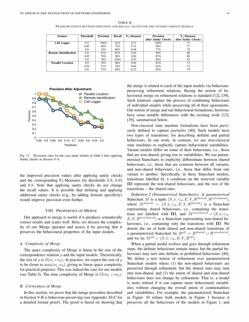
To compare the overall effectiveness of static matching,behavioural matching, and their combination, we computedtheir precision and recall for thresholds ranging from 0.95down to 0.5. The results are shown in Figure 16. As statedearlier in Section IV-C, threshold refers to the cutoff value usedfor determining the correspondence relation from the similaritydegrees. The three diagrams at the top of Figure 16 representthe precision values for the three case studies in Table I,and the three diagrams at the bottom of that figure representthe recall values for those case studies. For example, whenthreshold is set to 0.9, the precision values for the combined,static, and behavioural matchings for the remote identification
TO APPEAR IN IEEE TRANSACTIONS ON SOFTWARE ENGINEERING 12
Fig. 14. Relationship between the models in Figure 1.
Fig. 15. Merge with respect to the relationship in Figure 14.
TO APPEAR IN IEEE TRANSACTIONS ON SOFTWARE ENGINEERING 13
0%
13%
25%
38%
50%
63%
75%
88%
100%
0.95 0.9 0.85 0.8 0.75 0.7 0.65 0.6 0.55 0.5
Call LoggerP
recis
ion
Threshold
Threshold
Call Logger PrecisionCall Logger PrecisionCall Logger PrecisionCall Logger Precision Remote Identification PrecisionRemote Identification PrecisionRemote Identification Precision Parallel Location PrecisionParallel Location PrecisionParallel Location Precision
Static Behavioural Combined Static Behavioural Combined Static Behavioural Combined
0.95
0.9
0.85
0.8
0.75
0.7
0.65
0.6
0.55
0.5
0.95
0.9
0.85
0.8
0.75
0.7
0.65
0.6
0.55
0.5
0.95
0.9
0.85
0.8
0.75
0.7
0.65
0.6
0.55
0.5
0.64 0.35 1 0.6 0.4 0.83 0.5 0.3 0.75
0.43 0.25 1 0.5 0.24 0.81 0.33 0.15 0.7
0.44 0.12 0.8 0.48 0.22 0.79 0.28 0.1 0.51
0.45 0.18 0.53 0.44 0.25 0.7 0.24 0.12 0.53
0.44 0.17 0.42 0.43 0.26 0.57 0.21 0.09 0.34
0.39 0.2 0.27 0.4 0.28 0.55 0.19 0.18 0.32
0.3 0.15 0.22 0.38 0.2 0.39 0.19 0.1 0.14
0.25 0.16 0.24 0.35 0.32 0.42 0.19 0.12 0.22
0.2 0.1 0.12 0.22 0.23 0.26 0.18 0.08 0.13
0.17 0.1 0.17 0.17 0.18 0.24 0.12 0.05 0.12
Call Logger RecallCall Logger RecallCall Logger Recall Remote Identification RecallRemote Identification RecallRemote Identification Recall Parallel Location RecallParallel Location RecallParallel Location Recall
0.42 0.82 0.62 0.62 0.9 0.85 0.38 0.71 0.59
0.42 0.8 0.62 0.65 0.9 0.85 0.5 0.74 0.68
0.62 0.78 0.72 0.69 0.9 0.9 0.62 0.74 0.78
0.62 0.9 0.79 0.71 0.88 1 0.66 0.82 0.88
0.65 0.92 0.78 0.8 0.9 1 0.68 1 0.85
0.64 0.95 0.82 0.79 0.9 1 0.7 1 0.83
0.66 0.93 0.84 0.78 0.88 1 0.7 1 1
0.7 0.92 0.85 0.78 0.98 1 0.72 1 1
0.74 0.92 0.85 0.85 0.98 1 0.78 1 1
0.79 0.92 0.84 0.84 0.98 1 0.81 1 1
Call Logger Precisio2Call Logger Precisio2Call Logger Precisio2 Remote Identificaiton Precisio2Remote Identificaiton Precisio2Remote Identificaiton Precisio2 Parallel Location Precision2Parallel Location Precision2Parallel Location Precision2
1 0.9 0.88
1 0.9 0.85
0.9 0.85 0.62
0.77 0.8 0.65
0.62 0.72 0.5
0.5 0.68 0.45
0.35 0.54 0.3
0.35 0.59 0.35
0.25 0.45 0.25
0.28 0.4 0.23
0.7099236641221 0.8432270916335 0.6351674641148
0.7099236641221 0.8362348178138 0.6865384615385
0.7448275862069 0.8600806451613 0.663
0.678972972973 0.875 0.7212371134021
0.6066666666667 0.7990654205607 1.2222222222222
0.4883823529412 0.7857142857143 0.5420408163265
0.433125 0.6573033707865 1.109375
0.4601503759399 0.6847826086957 0.4583333333333
0.2807339449541 0.5131578947368 0.3095238095238
0.3630508474576 0.4864864864865 0.2903225806452
Call Logger Precision-RecallCall Logger Precision-RecallCall Logger Precision-Recall
CombinedCombined BehaviouralBehavioural StaticStatic
1 0.62 0.35 0.82 0.64 0.42
1 0.62 0.25 0.8 0.43 0.42
0.8 0.72 0.12 0.78 0.44 0.62
0.53 0.79 0.18 0.9 0.45 0.62
0.42 0.78 0.17 0.92 0.44 0.65
0.27 0.82 0.2 0.95 0.39 0.64
0.22 0.84 0.15 0.93 0.3 0.66
0.24 0.85 0.16 0.92 0.25 0.7
0.12 0.85 0.1 0.92 0.2 0.74
0.17 0.84 0.1 0.92 0.17 0.79
Remote Identification Precision-RecallRemote Identification Precision-RecallRemote Identification Precision-Recall
CombinedCombined BehaviouralBehavioural StaticStatic
0.83 0.85 0.4 0.9 0.6 0.62
0.81 0.85 0.24 0.9 0.5 0.65
0.79 0.9 0.22 0.9 0.48 0.69
0.7 1 0.25 0.88 0.44 0.71
0.57 1 0.26 0.9 0.43 0.8
0.55 1 0.28 0.9 0.4 0.79
0.39 1 0.2 0.88 0.38 0.78
0.42 1 0.32 0.98 0.35 0.78
0.26 1 0.23 0.98 0.22 0.85
0.24 1 0.18 0.98 0.17 0.84
Parallel Location Precision-RecallParallel Location Precision-RecallParallel Location Precision-Recall
CombinedCombined BehaviouralBehavioural StaticStatic
0.75 0.59 0.3 0.71 0.5 0.38
0.7 0.68 0.15 0.74 0.33 0.5
0.51 0.78 0.1 0.74 0.28 0.62
0.53 0.88 0.12 0.82 0.24 0.66
0.34 0.85 0.09 1 0.21 0.68
0.32 0.83 0.18 1 0.19 0.7
0.14 1 0.1 1 0.19 0.7
0.22 1 0.12 1 0.19 0.72
0.13 1 0.08 1 0.18 0.78
0.12 1 0.05 1 0.12 0.81
StaticBehaviouralCombined
0%
11%
23%
34%
45%
56%
68%
79%
90%
0.95 0.9 0.85 0.8 0.75 0.7 0.65 0.6 0.55 0.5
Remote Identification
Pre
cis
ion
Threshold
0%
10%
20%
30%
40%
50%
60%
70%
80%
0.95 0.9 0.85 0.8 0.75 0.7 0.65 0.6 0.55 0.5
Parallel Location
Pre
cis
ion
Threshold
0%
13%
25%
38%
50%
63%
75%
88%
100%
0.95 0.9 0.85 0.8 0.75 0.7 0.65 0.6 0.55 0.5
Call Logger
Recall
Threshold
0%
13%
25%
38%
50%
63%
75%
88%
100%
0.95 0.9 0.85 0.8 0.75 0.7 0.65 0.6 0.55 0.5
Remote Identification
Recall
Threshold
0%
13%
25%
38%
50%
63%
75%
88%
100%
0.95 0.9 0.85 0.8 0.75 0.7 0.65 0.6 0.55 0.5
Parallel Location
Recall
Threshold
0
0.1
0.2
0.3
0.4
0.5
0.6
0.7
0.8
0.9
1
0.95 0.9 0.85 0.8 0.75 0.7 0.65 0.6 0.55 0.5
Precision After Adjustment
Pre
cis
ion
Threshold
Parallel LocationRemote IdentificatoinCall Logger
Fig. 16. Results of static, behavioural, and combined matching.
case study are 81%, 50%, and 24%, respectively. In our studywe observed that among the three pairs of model variants, theparallel location variants had the largest overlap, i.e., the high-est number of tuples in their correspondence relation, whilethe call logger variants had the least overlap. Furthermore, thehierarchy trees of the parallel location variants were the mostsimilar in terms of the height of the hierarchy trees.
In the studied models, states with typographically similarnames were likely to correspond. Hence, typographic matchingand, by extension, static matching have high precision. How-ever, static matching misses several correct matches, and hencehas low recall. Behavioural matching, in contrast, has lowerprecision, but high recall. When the threshold is set reasonablyhigh, combined matching has precision rates higher than thoseof static and behavioural matching on their own. This indicatesthat static and behavioural matching are filtering out eachother’s false positives. Recall remains high in the combinedapproach, as static matching and behavioural matching findmany complimentary high-quality matches.
The results in Figure 16 show that for each of the studiedmodels, our combined matcher can achieve high precision(above 75%) for some thresholds, and high recall (above95%) for some other thresholds. To be able to compare theprecision and recall values across different experiments, weuse another metric known as F-Measure [36] which computesthe harmonic mean of recall and precision and therefore isoften used for comparative purposes. In this paper, we use adefinition of F-Measure, known as F2-Measure, which weighsrecall values more highly than precision.
F2-Measure =3× Precision× Recall
(2× Precision) + Recall
This weighting is appropriate in our domain where it is
important to recall as many of the correct matches as possible.Table II (columns 1 to 5 from left) presents recall, precision
and threshold values that yield maximal F2-Measure valuesacross our three case studies. The maximal F2-Measure valuesare obtained when threshold is set between 0.8 and 0.9. Theprecision values in the table range between 51% and 100%,and their corresponding recall values – between 62% and100%.
As we anticipated, trying to improve our matcher’s precisionand recall by tweaking the heuristics behind it resulted inimproving one at the expense of the other. For instance,when we let the behavioural heuristics run for relatively fewiterations (< 10), the result has higher precision but lowerrecall because more iterations are needed to properly propagatethe similarity values in order to identify all of the correctmatches. On the other hand, running the behavioural heuristicsfor a relatively large number of iterations (> 100) causesa higher recall but a lower precision. Instead, we suggestthe following strategy aimed at improving both precision andrecall: (1) adjust the matcher’s heuristics to optimize recall;and (2) identify and prune false positives using the sanitychecks defined in Section V-A. For example, applying theseto the relation in Figure 8(b) results in the removal of thetuples (s1, t0) and (s1, t1) (see Figure 8(c)). This leads toan increase in precision from 8/14 (57%) to 8/12 (67%) andrecall remains the same, i.e., 8/8 (100%). Figure 17 showsthe precision values of the combined matcher for the threestudied models after applying the sanity checks. Note that thethree curves in this figure correspond to the three case studies,rather than to the static/behavioural/combined algorithms as inFigure 16. Compared to the results in Figure 16, this method-ology yields a 5%-25% improvement in precision across thedifferent thresholds. The last two columns in Table II represent
TO APPEAR IN IEEE TRANSACTIONS ON SOFTWARE ENGINEERING 14
TABLE IITRADEOFF POINTS BETWEEN PRECISION AND RECALL VALUES FOR THE STUDIED VARIANT MODELS.
Feature Threshold Precision Recall F2-Measure Precision F2-Measureafter Sanity Checks after Sanity Checks
Call Logger 0.9 100% 62% 0.71 100% .710.85 80% 72% 0.74 90% .770.8 54% 80% 0.68 77% .78
Remote Identification 0.9 81% 85% 0.84 90% .860.85 79% 90% 0.86 85% .880.8 70% 100% 0.87 80% .92
Parallel Location 0.9 70% 68% 0.69 85% .730.85 51% 78% 0.66 62% .720.8 53% 88% 0.72 65% .79
0%
13%
25%
38%
50%
63%
75%
88%
100%
0.95 0.9 0.85 0.8 0.75 0.7 0.65 0.6 0.55 0.5
Call Logger
Pre
cis
ion
Threshold
Threshold
Call Logger PrecisionCall Logger PrecisionCall Logger PrecisionCall Logger Precision Remote Identification PrecisionRemote Identification PrecisionRemote Identification Precision Parallel Location PrecisionParallel Location PrecisionParallel Location Precision
Static Behavioural Combined Static Behavioural Combined Static Behavioural Combined
0.95
0.9
0.85
0.8
0.75
0.7
0.65
0.6
0.55
0.5
0.95
0.9
0.85
0.8
0.75
0.7
0.65
0.6
0.55
0.5
0.95
0.9
0.85
0.8
0.75
0.7
0.65
0.6
0.55
0.5
0.64 0.35 1 0.6 0.4 0.83 0.5 0.3 0.75
0.43 0.25 1 0.5 0.24 0.81 0.33 0.15 0.7
0.44 0.12 0.8 0.48 0.22 0.79 0.28 0.1 0.51
0.45 0.18 0.53 0.44 0.25 0.7 0.24 0.12 0.53
0.44 0.17 0.42 0.43 0.26 0.57 0.21 0.09 0.34
0.39 0.2 0.27 0.4 0.28 0.55 0.19 0.18 0.32
0.3 0.15 0.22 0.38 0.2 0.39 0.19 0.1 0.14
0.25 0.16 0.24 0.35 0.32 0.42 0.19 0.12 0.22
0.2 0.1 0.12 0.22 0.23 0.26 0.18 0.08 0.13
0.17 0.1 0.17 0.17 0.18 0.24 0.12 0.05 0.12
Call Logger RecallCall Logger RecallCall Logger Recall Remote Identification RecallRemote Identification RecallRemote Identification Recall Parallel Location RecallParallel Location RecallParallel Location Recall
0.42 0.82 0.62 0.62 0.9 0.85 0.38 0.71 0.59
0.42 0.8 0.62 0.65 0.9 0.85 0.5 0.74 0.68
0.62 0.78 0.72 0.69 0.9 0.9 0.62 0.74 0.78
0.62 0.9 0.79 0.71 0.88 1 0.66 0.82 0.88
0.65 0.92 0.78 0.8 0.9 1 0.68 1 0.85
0.64 0.95 0.82 0.79 0.9 1 0.7 1 0.83
0.66 0.93 0.84 0.78 0.88 1 0.7 1 1
0.7 0.92 0.85 0.78 0.98 1 0.72 1 1
0.74 0.92 0.85 0.85 0.98 1 0.78 1 1
0.79 0.92 0.84 0.84 0.98 1 0.81 1 1
Call Logger Precisio2Call Logger Precisio2Call Logger Precisio2 Remote Identificaiton Precisio2Remote Identificaiton Precisio2Remote Identificaiton Precisio2 Parallel Location Precision2Parallel Location Precision2Parallel Location Precision2
1 0.9 0.88
1 0.9 0.85
0.9 0.85 0.62
0.77 0.8 0.65
0.62 0.72 0.5
0.5 0.68 0.45
0.35 0.54 0.3
0.35 0.59 0.35
0.25 0.45 0.25
0.28 0.4 0.23
0.7099236641221 0.8432270916335 0.6351674641148
0.7099236641221 0.8362348178138 0.6865384615385
0.7448275862069 0.8600806451613 0.663
0.678972972973 0.875 0.7212371134021
0.6066666666667 0.7990654205607 1.2222222222222
0.4883823529412 0.7857142857143 0.5420408163265
0.433125 0.6573033707865 1.109375
0.4601503759399 0.6847826086957 0.4583333333333
0.2807339449541 0.5131578947368 0.3095238095238
0.3630508474576 0.4864864864865 0.2903225806452
Call Logger Precision-RecallCall Logger Precision-RecallCall Logger Precision-Recall
CombinedCombined BehaviouralBehavioural StaticStatic
1 0.62 0.35 0.82 0.64 0.42
1 0.62 0.25 0.8 0.43 0.42
0.8 0.72 0.12 0.78 0.44 0.62
0.53 0.79 0.18 0.9 0.45 0.62
0.42 0.78 0.17 0.92 0.44 0.65
0.27 0.82 0.2 0.95 0.39 0.64
0.22 0.84 0.15 0.93 0.3 0.66
0.24 0.85 0.16 0.92 0.25 0.7
0.12 0.85 0.1 0.92 0.2 0.74
0.17 0.84 0.1 0.92 0.17 0.79
Remote Identification Precision-RecallRemote Identification Precision-RecallRemote Identification Precision-Recall
CombinedCombined BehaviouralBehavioural StaticStatic
0.83 0.85 0.4 0.9 0.6 0.62
0.81 0.85 0.24 0.9 0.5 0.65
0.79 0.9 0.22 0.9 0.48 0.69
0.7 1 0.25 0.88 0.44 0.71
0.57 1 0.26 0.9 0.43 0.8
0.55 1 0.28 0.9 0.4 0.79
0.39 1 0.2 0.88 0.38 0.78
0.42 1 0.32 0.98 0.35 0.78
0.26 1 0.23 0.98 0.22 0.85
0.24 1 0.18 0.98 0.17 0.84
Parallel Location Precision-RecallParallel Location Precision-RecallParallel Location Precision-Recall
CombinedCombined BehaviouralBehavioural StaticStatic
0.75 0.59 0.3 0.71 0.5 0.38
0.7 0.68 0.15 0.74 0.33 0.5
0.51 0.78 0.1 0.74 0.28 0.62
0.53 0.88 0.12 0.82 0.24 0.66
0.34 0.85 0.09 1 0.21 0.68
0.32 0.83 0.18 1 0.19 0.7
0.14 1 0.1 1 0.19 0.7
0.22 1 0.12 1 0.19 0.72
0.13 1 0.08 1 0.18 0.78
0.12 1 0.05 1 0.12 0.81
StaticBehaviouralCombined
0%
11%
23%
34%
45%
56%
68%
79%
90%
0.95 0.9 0.85 0.8 0.75 0.7 0.65 0.6 0.55 0.5
Remote Identification
Pre
cis
ion
Threshold
0%
10%
20%
30%
40%
50%
60%
70%
80%
0.95 0.9 0.85 0.8 0.75 0.7 0.65 0.6 0.55 0.5
Parallel Location
Pre
cis
ion
Threshold
0%
13%
25%
38%
50%
63%
75%
88%
100%
0.95 0.9 0.85 0.8 0.75 0.7 0.65 0.6 0.55 0.5
Call Logger
Recall
Threshold
0%
13%
25%
38%
50%
63%
75%
88%
100%
0.95 0.9 0.85 0.8 0.75 0.7 0.65 0.6 0.55 0.5
Remote Identification
Recall
Threshold
0%
13%
25%
38%
50%
63%
75%
88%
100%
0.95 0.9 0.85 0.8 0.75 0.7 0.65 0.6 0.55 0.5
Parallel Location
Recall
Threshold
0
0.1
0.2
0.3
0.4
0.5
0.6
0.7
0.8
0.9
1
0.95 0.9 0.85 0.8 0.75 0.7 0.65 0.6 0.55 0.5
Precision After Adjustment
Pre
cis
ion
Threshold
Parallel LocationRemote IdentificatoinCall Logger
Fig. 17. Precisions rates for the case study models in Table I after applyingSanity checks in Section V-A.
the improved precision values after applying sanity checksand the corresponding F2-Measures for thresholds 0.9, 0.85and 0.8. Note that applying sanity checks do not changethe recall values. It is possible that defining and applyingadditional sanity checks (e.g., by adding domain specificity)would improve precision even further.
VIII. PROPERTIES OF MERGE
Our approach to merge is useful if it produces semanticallycorrect results and scales well. Here, we discuss the complex-ity of our Merge operator and assess it by proving that itpreserves the behavioural properties of the input models.
A. Complexity of Merge
The space complexity of Merge is linear in the size of thecorrespondence relation ρ and the input models. Theoretically,the size of ρ is O(n1×n2). In practice, we expect the size of ρto be closer to max(n1, n2), giving us linear space complexityfor practical purposes. This was indeed the case for our models(see Table I). The time complexity of Merge is O(m1×m2).
B. Correctness of Merge
In this section, we prove that the merge procedure describedin Section V-B is behaviour-preserving (see Appendix XI-C fora detailed formal proof). The proof is based on showing that
the merge is related to each of the input models via behaviour-preserving refinement relations. Basing the notion of be-havioural merge on refinement relations is standard [12], [39].Such relations capture the process of combining behavioursof individual models while preserving all of their agreements.Our notion of merge and our behavioural formalisms, however,have some notable differences with the existing work [12],[39], summarized below.
Non-classical state machine formalisms have been previ-ously defined to capture partiality [40]. Such models havetwo types of transitions: for describing definite and partialbehaviours. In our work, in contrast, we use non-classicalstate machines to explicitly capture behavioural variabilities.Variant models differ on some of their behaviours, i.e., thosethat are non-shared, giving rise to variabilities. We use param-eterized Statecharts to explicitly differentiate between sharedbehaviours, i.e., those that are common between all variants,and non-shared behaviours, i.e., those that differ from onevariant to another. Specifically, in these Statechart models,transitions labelled by a condition on the reserved variableID represent the non-shared behaviours, and the rest of thetransitions – the shared ones.
Definition 2 (Parameterized Statecharts): A parameterizedStatechart M is a tuple (S, s, <h, E, V,R
shared , Rnonshared),where M shared = (S, s, <h, E, V,R
shared) is a Statechartrepresenting shared behaviours, i.e., containing the transi-tions not labelled with ID, and Mnonshared = (S, s, <h,E, V,Rnonshared) is a Statechart representing non-shared be-haviours, i.e., containing only the transitions with ID. Wedenote the set of both shared and non-shared transitions ofa parameterized Statechart by Rall = Rshared ∪ Rnonshared ,and we let Mall = (S, s, <h, E, V,R
all).When a partial model evolves and goes through refinement
steps, the definite behaviours remain intact, but the partial be-haviours may turn into definite or prohibited behaviours [40].We define a new notion of refinement over parameterizedStatechart models where (1) the non-shared behaviours arepreserved through refinement, but the shared ones may turninto non-shared, and (2) the union of shared and non-sharedbehaviours does not change by refinement. That is, a modelis more refined if it can capture more behavioural variabil-ities without changing the overall union of commonalitiesand variabilities. For example, the parameterized Statechartin Figure 10 refines both models in Figure 1 because itpreserves all the behaviours of the models in Figure 1, and
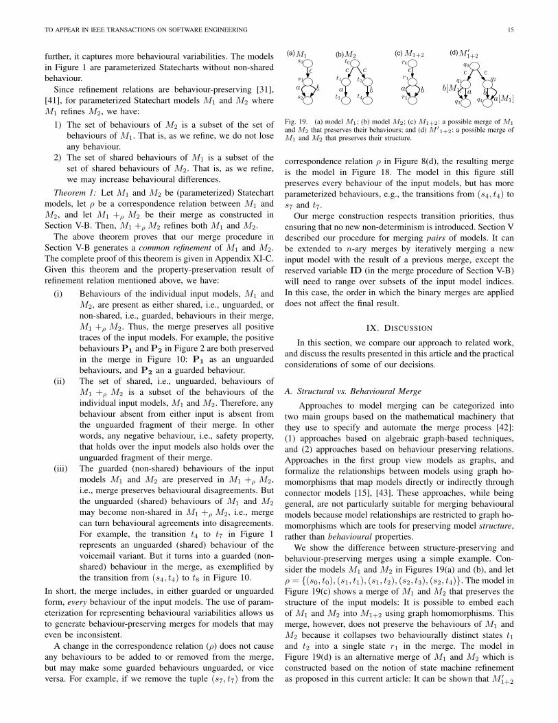
TO APPEAR IN IEEE TRANSACTIONS ON SOFTWARE ENGINEERING 15
further, it captures more behavioural variabilities. The modelsin Figure 1 are parameterized Statecharts without non-sharedbehaviour.
Since refinement relations are behaviour-preserving [31],[41], for parameterized Statechart models M1 and M2 whereM1 refines M2, we have:
1) The set of behaviours of M2 is a subset of the set ofbehaviours of M1. That is, as we refine, we do not loseany behaviour.
2) The set of shared behaviours of M1 is a subset of theset of shared behaviours of M2. That is, as we refine,we may increase behavioural differences.
Theorem 1: Let M1 and M2 be (parameterized) Statechartmodels, let ρ be a correspondence relation between M1 andM2, and let M1 +ρ M2 be their merge as constructed inSection V-B. Then, M1 +ρM2 refines both M1 and M2.
The above theorem proves that our merge procedure inSection V-B generates a common refinement of M1 and M2.The complete proof of this theorem is given in Appendix XI-C.Given this theorem and the property-preservation result ofrefinement relation mentioned above, we have:
(i) Behaviours of the individual input models, M1 andM2, are present as either shared, i.e., unguarded, ornon-shared, i.e., guarded, behaviours in their merge,M1 +ρ M2. Thus, the merge preserves all positivetraces of the input models. For example, the positivebehaviours P1 and P2 in Figure 2 are both preservedin the merge in Figure 10: P1 as an unguardedbehaviours, and P2 an a guarded behaviour.
(ii) The set of shared, i.e., unguarded, behaviours ofM1 +ρ M2 is a subset of the behaviours of theindividual input models, M1 and M2. Therefore, anybehaviour absent from either input is absent fromthe unguarded fragment of their merge. In otherwords, any negative behaviour, i.e., safety property,that holds over the input models also holds over theunguarded fragment of their merge.
(iii) The guarded (non-shared) behaviours of the inputmodels M1 and M2 are preserved in M1 +ρ M2,i.e., merge preserves behavioural disagreements. Butthe unguarded (shared) behaviours of M1 and M2
may become non-shared in M1 +ρ M2, i.e., mergecan turn behavioural agreements into disagreements.For example, the transition t4 to t7 in Figure 1represents an unguarded (shared) behaviour of thevoicemail variant. But it turns into a guarded (non-shared) behaviour in the merge, as exemplified bythe transition from (s4, t4) to t8 in Figure 10.
In short, the merge includes, in either guarded or unguardedform, every behaviour of the input models. The use of param-eterization for representing behavioural variabilities allows usto generate behaviour-preserving merges for models that mayeven be inconsistent.
A change in the correspondence relation (ρ) does not causeany behaviours to be added to or removed from the merge,but may make some guarded behaviours unguarded, or viceversa. For example, if we remove the tuple (s7, t7) from the
(a) (b) (c) (d)
c
a b
c c
a b
M1 M2 M1+2 M ′1+2
s0
s1
s2
t0
t1 t2
t3 t4
c c
a ba[M1]
b[M1]
q0
q1q2
q3q4
r0
r1
r2
c
ba
Fig. 19. (a) model M1; (b) model M2; (c) M1+2: a possible merge of M1
and M2 that preserves their behaviours; and (d) M ′1+2: a possible merge ofM1 and M2 that preserves their structure.
correspondence relation ρ in Figure 8(d), the resulting mergeis the model in Figure 18. The model in this figure stillpreserves every behaviour of the input models, but has moreparameterized behaviours, e.g., the transitions from (s4, t4) tos7 and t7.
Our merge construction respects transition priorities, thusensuring that no new non-determinism is introduced. Section Vdescribed our procedure for merging pairs of models. It canbe extended to n-ary merges by iteratively merging a newinput model with the result of a previous merge, except thereserved variable ID (in the merge procedure of Section V-B)will need to range over subsets of the input model indices.In this case, the order in which the binary merges are applieddoes not affect the final result.
IX. DISCUSSION
In this section, we compare our approach to related work,and discuss the results presented in this article and the practicalconsiderations of some of our decisions.
A. Structural vs. Behavioural Merge
Approaches to model merging can be categorized intotwo main groups based on the mathematical machinery thatthey use to specify and automate the merge process [42]:(1) approaches based on algebraic graph-based techniques,and (2) approaches based on behaviour preserving relations.Approaches in the first group view models as graphs, andformalize the relationships between models using graph ho-momorphisms that map models directly or indirectly throughconnector models [15], [43]. These approaches, while beinggeneral, are not particularly suitable for merging behaviouralmodels because model relationships are restricted to graph ho-momorphisms which are tools for preserving model structure,rather than behavioural properties.
We show the difference between structure-preserving andbehaviour-preserving merges using a simple example. Con-sider the models M1 and M2 in Figures 19(a) and (b), and letρ = {(s0, t0), (s1, t1), (s1, t2), (s2, t3), (s2, t4)}. The model inFigure 19(c) shows a merge of M1 and M2 that preserves thestructure of the input models: It is possible to embed eachof M1 and M2 into M1+2 using graph homomorphisms. Thismerge, however, does not preserve the behaviours of M1 andM2 because it collapses two behaviourally distinct states t1and t2 into a single state r1 in the merge. The model inFigure 19(d) is an alternative merge of M1 and M2 which isconstructed based on the notion of state machine refinementas proposed in this current article: It can be shown that M ′1+2
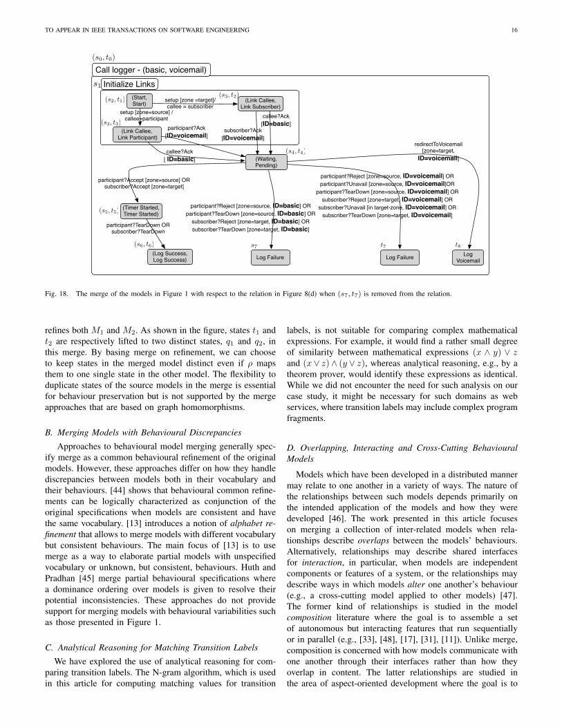
TO APPEAR IN IEEE TRANSACTIONS ON SOFTWARE ENGINEERING 16
(Link Callee, Link Subscriber)
(Link Callee, Link Participant)
(Waiting, Pending)
(Timer Started, Timer Started)
Log Failure(Log Success, Log Success)
setup [zone =target]/callee = subscriber
setup [zone=source] /callee=participant
participant?Ack [ID=voicemail]
subscriber?Ack[ID=voicemail]
redirectToVoicemail[zone=target,ID=voicemail]
participant?Reject [zone=source, ID=basic] ORparticipant?TearDown [zone=source, ID=basic] OR
subscriber?Reject [zone=target, ID=basic] ORsubscriber?TearDown [zone=target, ID=basic]
participant?TearDown ORsubscriber?TearDown
participant?Accept [zone=source] ORsubscriber?Accept [zone=target]
Log Voicemail
(s0, t0)
callee?Ack[ID=basic]
callee?Ack[ ID=basic]
Call logger - (basic, voicemail)
(Start, Start)
Initialize Linkss1
(s2, t1)(s3, t2)
(s3, t3)
(s4, t4)
(s5, t5)
(s6, t6) t8
Log Failure
participant?Reject [zone=source, ID=voicemail] ORparticipant?Unavail [zone=source, ID=voicemail]OR
participant?TearDown [zone=source, ID=voicemail] ORsubscriber?Reject [zone=target, ID=voicemail] OR
subscriber?Unavail [in target-zone, ID=voicemail] ORsubscriber?TearDown [zone=target, ID=voicemail]
s7 t7
Fig. 18. The merge of the models in Figure 1 with respect to the relation in Figure 8(d) when (s7, t7) is removed from the relation.
refines both M1 and M2. As shown in the figure, states t1 andt2 are respectively lifted to two distinct states, q1 and q2, inthis merge. By basing merge on refinement, we can chooseto keep states in the merged model distinct even if ρ mapsthem to one single state in the other model. The flexibility toduplicate states of the source models in the merge is essentialfor behaviour preservation but is not supported by the mergeapproaches that are based on graph homomorphisms.
B. Merging Models with Behavioural Discrepancies
Approaches to behavioural model merging generally spec-ify merge as a common behavioural refinement of the originalmodels. However, these approaches differ on how they handlediscrepancies between models both in their vocabulary andtheir behaviours. [44] shows that behavioural common refine-ments can be logically characterized as conjunction of theoriginal specifications when models are consistent and havethe same vocabulary. [13] introduces a notion of alphabet re-finement that allows to merge models with different vocabularybut consistent behaviours. The main focus of [13] is to usemerge as a way to elaborate partial models with unspecifiedvocabulary or unknown, but consistent, behaviours. Huth andPradhan [45] merge partial behavioural specifications wherea dominance ordering over models is given to resolve theirpotential inconsistencies. These approaches do not providesupport for merging models with behavioural variabilities suchas those presented in Figure 1.
C. Analytical Reasoning for Matching Transition Labels
We have explored the use of analytical reasoning for com-paring transition labels. The N-gram algorithm, which is usedin this article for computing matching values for transition
labels, is not suitable for comparing complex mathematicalexpressions. For example, it would find a rather small degreeof similarity between mathematical expressions (x ∧ y) ∨ zand (x∨ z)∧ (y ∨ z), whereas analytical reasoning, e.g., by atheorem prover, would identify these expressions as identical.While we did not encounter the need for such analysis on ourcase study, it might be necessary for such domains as webservices, where transition labels may include complex programfragments.
D. Overlapping, Interacting and Cross-Cutting BehaviouralModels
Models which have been developed in a distributed mannermay relate to one another in a variety of ways. The nature ofthe relationships between such models depends primarily onthe intended application of the models and how they weredeveloped [46]. The work presented in this article focuseson merging a collection of inter-related models when rela-tionships describe overlaps between the models’ behaviours.Alternatively, relationships may describe shared interfacesfor interaction, in particular, when models are independentcomponents or features of a system, or the relationships maydescribe ways in which models alter one another’s behaviour(e.g., a cross-cutting model applied to other models) [47].The former kind of relationships is studied in the modelcomposition literature where the goal is to assemble a setof autonomous but interacting features that run sequentiallyor in parallel (e.g., [33], [48], [17], [31], [11]). Unlike merge,composition is concerned with how models communicate withone another through their interfaces rather than how theyoverlap in content. The latter relationships are studied inthe area of aspect-oriented development where the goal is to
TO APPEAR IN IEEE TRANSACTIONS ON SOFTWARE ENGINEERING 17
weave cross-cutting concerns into a base system (e.g., [49],[50], [51]). The focus of this article was on relationshipsthat capture overlaps between model behaviours, and not onsituations where model relationships describe interactions orcross-cutting aspects.
E. Model Matching Techniques
Approaches to model matching can be exact or approx-imate. Exact matching is concerned with finding structuralor behavioural conformance relations between models. Graphhomomorphisms are examples of the former, whereas simu-lation and bisimulation relationships – of the latter. Findingexact correspondences between models has applications inmany fields including graph rewriting, pattern recognition,program analysis, and compiler optimization. However, itis not very useful for matching distributed models becausethe vocabularies and behaviours of these models seldom fittogether in an exact way, and thus, exact conformance relationsbetween these models are unlikely to be found.
Most domains use heuristic techniques for matching. Thesetechniques yield values denoting a likelihood of correspon-dence between elements of different models. In databasedesign, finding correspondences between database schemata isreferred to as schema matching [52]. State-of-the-art schemamatchers, such as Protoplasm [9], combine several heuristicsfor computing similarities between schema elements. Ourtypographic and linguistic heuristics (Section IV-A) are verysimilar to those used in schema matching, but our otherheuristics are tailored to behavioural models.
Several approaches to matching have been proposed insoftware engineering. Maiden and Sutcliffe [6] employ heuris-tic reasoning for finding analogies between a problem de-scription and already existing domain abstractions. Ryan andMathews [53] use approximate graph matching for findingoverlaps between concept graphs. Alspaugh et. al. [54] pro-pose term matching based on project glossaries for findingsimilarities between textual scenarios. Mandelin et. al. [4]combine diagrammatic and syntactic heuristics for findingmatches between architecture models. Xing and Stroulia [55]use heuristic-based name-similarity and structure-similaritymatchers to identify conceptually similar entities in UMLclass diagrams. None of these approaches were specificallydesigned for behavioural models and are either inapplicableor unsuitable for matching Statechart models.
Some matching approaches deal with behavioural mod-els of a different kind. For example, Kelter and Schmidt[56] discuss differencing mechanisms specifically designedfor UML Statecharts. This work assumes that models aredeveloped centrally within a unified modelling environment.Other approaches apply to independently-developed models.Lohmann [57] and Zisman et. al. [8] define similarity measuresbetween web-services to identify candidate services to replacea service in use when it becomes unavailable or unsuitabledue to a change. Quante and Koschke [58] propose similaritymeasures between finite state automata generated by differentreverse engineering mechanisms to compare the effectivenessof these mechanisms. Bogdanov and Walkinshaw [59] provide
an algorithm for comparing LTSs without relying on the initialstate or any particular states of the underlying models as thereference point. None of these are applicable both to ourparticular purpose (comparing different versions of the samefeature), and to our particular class of models (Statechartsmodels). Further, the evaluation of our matching technique istargeted at behavioural models built in the telecommunicationdomain. To our knowledge, the usefulness and effectiveness ofmodel matching have not been studied in this context before.
In computer science theory, several notions of behaviouralconformance have been proposed to capture the behaviouralsimilarity between models with quantitative features such astime or probability [60]. For these models, a discrete notion ofsimilarity, i.e., models are either equivalent or they are not, isnot helpful because minor changes in the quantitative data maycause equivalent models to become inequivalent, even if thedifference between their behaviours is very minor. Therefore,instead of equivalences that result in a binary answer, oneneeds to use relations that can differentiate between slightlydifferent and completely different models. Examples of suchrelations are stochastic or Markovian notions of behaviouralsimilarity (e.g., [61], [62]). Our formulation of behaviouralsimilarity (Section IV-B) is analogous to these similarityrelations. The goal of this work is to define a distance metricover the space of (quantitative) reactive processes and studythe mathematical properties of the metric. Our goal, instead,is to obtain a similarity measure that can detect pairs of stateswith a high degree of behavioural similarity.
F. Model Merging Techniques
Model merging spans several application areas. In databasedesign, merge is an important step for producing a schemacapturing the data requirements of all the stakeholders [2].Software engineering deals extensively with model merging –several papers study the subject in specific domains, includingearly requirements [15], static UML diagrams [63], [14],[64], [65], [66], and declarative specifications [67]. None ofthese were specifically designed for behavioural models andare either inapplicable or unsuitable for matching Statechartmodels. We compared our work with existing approaches formerging behavioural models in Section IX-B.
There has also been work on defining languages for modelmerging, e.g., the Epsilon Merging Language (EML) [10] andAtlas Model Management Architecture (AMMA) [68]. EMLis a rule-based language for merging models with the same ordifferent meta-models. The language distinguishes four phasesin the merge process and provides flexible constructs fordefining the rules that should be applied in each phase. AMMAfacilitates modelling tasks such as merging using model trans-formation languages defined between different meta-models.Despite their versatility, the current version of EML andAMMA do not formalize the conditions and consequencesof applying the merge rules, and hence, in contrast to ourapproach, do not provide a formal characterization of themerge operation when applied to behavioural models.
In this article, we focused on the application of behaviouralmerge as a way to reconcile models developed independently.
TO APPEAR IN IEEE TRANSACTIONS ON SOFTWARE ENGINEERING 18
Behavioural merge operation may arise in several other relatedareas, including program integration [69] and merging declar-ative specifications [67]. These approaches share the samegeneral motivation with our work which is preservation ofsemantics and support for handling inconsistencies. However,they are not targeted at consolidating variant specifications,and further do not use Statecharts as the underlying notation.
Several approaches to variability modelling have been pro-posed in software maintenance and product line engineering.For example, [70] provides an elaborate view of modellingvariability in use-cases by distinguishing between aspectsessential for satisfying customers’ needs and those related tothe technical realization of variability. Our merge operatormakes use of parameterization for representing variabilitiesbetween different models. This is a common technique inmodelling behavioural variability in Statechart models [34].A similar parameterization technique has been used in [71]for capturing variability in Software Cost Reduction (SCR)tables [72].
In requirements and early design model merging, discrep-ancies are often treated as inconsistencies [73], [12], [15].Some of these approaches require that only consistent modelsbe merged [12]. Others tolerate inconsistency, and can rep-resent the inconsistencies explicitly in the resulting mergedmodel [73], [15]. Our work is similar to the latter groupas we explicitly model variabilities between models usingparameterization.
Several approaches provide guidelines and methodologiesfor building product lines out of legacy systems (e.g., [74]).Most of these approaches rely on a manual review of code,design and documentation of the system that can be time-consuming. The ability to mine legacy product lines andautomate their translation to a product line model capturingcommonalities and variabilities is a necessity. Clearly, suchtranslations should preserve the set and behavior of existingproducts, and, potentially, allow identification and addition ofnew products to the product line. Our approach can providea basis for behaviour-preserving refactoring of product linemodels from a set of existing (legacy) model variants [75].
G. Handling Additional Statechart FeaturesOur approach to Match and Merge can be systematically
extended to handle Statchart models with features other thanthose discussed in the paper. The general strategy for im-plementing such extensions is (1) to modify Definition 1 toincorporate the new features in the Statechart base notation,(2) to identify the additional sanity conditions (to be addedto those defined in Section V-A) so that the new features inthe original models are properly lifted to the merge, and (3)to modify the Merge algorithm in Section V-B to deal withshared aspects of the input models so that the merge remainssemantically sound. For example, one possible solution is toconstrain the model relationships via additional sanity checksso that the new features always fall in the non-shared parts ofthe input models. Although this solution works for arbitraryfeatures, it is too conservative. A better way is to studythe features one by one to identify less constraining sanityconditions for each. Below, we include two examples:
• State entry/exit/in/during actions. For input modelswith state actions, we constrain the relationships so thatthey can only be one-to-one, i.e., a state in one modelcannot be mapped to more than one state in the othermodel. This ensures that only one copy of every stateaction in the input models is lifted to the merge, andhence, these actions are executed the same number oftimes in the merge as in the input models. As observedin a study reported in [76], it is very common for modelsto be related via one-to-one relationships, so this is not alimiting restriction.
• Internal events. In this paper, we assumed that the inputmodels do not include internal events. That is, a transitiontriggered by an external event cannot produce internalevents that may, in turn, trigger other transitions (seeSection III). Our approach can handle internal events ifthe following two conditions hold: (1) The sanity checksare extended to ensure that the relationships betweenstates in the original models are one-to-one. Hence, se-quences of internal events are executed the same numberof times in the merge as in the input models. (2) Thedefinition of shared transitions in the merge algorithm inSection V-B is changed so that a pair of shared transitionshas identical actions, i.e., α = α′, as well as identicalevents, conditions, and priority. These shared transitionsare replaced in the merged model with one transition withan action α. Since the action on the transition in the mergeis the same as in the corresponding transitions in the inputmodels, the sequences of internal events generated in themerge by α are the same as in each of the input models.
Optionally, when extending the approach with additionalStatechart features, we can also augment the existing Matchheuristics with new heuristics designed specifically for thesenew features. For example, we can choose to compute sim-ilarity values based on the state entry/exit/in/during actionsand use these values to initialize the behavioural matchingin Section IV-B, i.e., we can consider these values to bethe behavioural matching similarities at iteration zero (thisapproach is implemented in [75]).
H. Practical Limitations
Our work has a number of limitations which we list below.
Evaluation. Our evaluation in Section VII may not be acomprehensive assessment of the effectiveness of our Matchoperator: Firstly, in our evaluation, we assume that it ispossible to find a matching relationship which is agreeableto all users. In practice, this may not be the case [3]. A morecomprehensive evaluation would require several independentsubjects to provide their desired correspondence relations,and use these for computing an average precision and recall.Secondly, matching results can be improved by proper userguidance, which we did not measure here. More specifically, inSection VII, we evaluated Match as a fully automatic operator.In practice, it might be reasonable to use Match interactively,with the user seeding it with some of the more obviousrelations, and pruning incorrect relations iteratively. We expect
TO APPEAR IN IEEE TRANSACTIONS ON SOFTWARE ENGINEERING 19
that such an approach will improve accuracy. Alternatively,a developer might prefer to assess the output of the Matchoperator by computing merge and inspecting the resultingmodel for validity. This way, each correspondence relationis treated as a hypothesis for how the models should becombined, to be adjusted if the resulting merge does not makesense. We plan to investigate the feasibility of this approachfurther.
Scalability and usability. Discussions in Sections VII-A andVIII-A show that the computational complexity of our opera-tors is not high. Since the space complexity of merge is linearin the size of the input models, the size of the merge does notgrow as rapidly as the size of (parallel) compositions [33], andhence, issues such as the state-explosion problem [33] do notarise in our work. In our evaluation and experimentation withthe Match and Merge operators, the actual running times ofour algorithms were also negligible.
Although our matching and merging algorithms scale wellin terms of computational efficiency and space usage, thereare some issues regarding usability of our approach that maylimit its applicability to large models. In particular, currentlyTReMer+ cannot preserve the layout of the source models, andignores all their visual cues during merge. We plan to addressthis issue in the future. Another problem is the representa-tion of model relationships. Visual representations are veryappealing but they may not scale well for complex operationalmodels such as large executable Statecharts. For such models,it should be possible to express relationships symbolicallyusing logical formulas or regular expressions. This may lead toa more compact and comprehensible representation of modelcorrespondences.
X. CONCLUSIONS AND FUTURE WORK
In this article, we presented an approach to matching andmerging of Statechart models. Our Match operator includesheuristics that use both static and behavioural properties tomatch pairs of states in the input models. Our evaluations showthat this combination produces higher precision than relyingon static or behavioural properties alone. Our Merge operatorproduces a combined model in which variant behaviours ofthe input models are parameterized using guards on theirtransitions. The result is a merge that preserves the temporalproperties of the input models. We have also developed atool that implements both our Merge and Match operators andenables seamless application of the two.
While our evaluation results demonstrate the effectivenessof our approach, its practical utility can only be assessed bymore extensive empirical studies. The value of our tool islikely to depend on factors such as the size and complexityof the models, the user’s familiarity with the models, and theuser’s subjective judgment of the matching results. Our Mergeoperator only applies to hierarchical state machine models.Extending it to behavioural models described in differentnotations, i.e., heterogeneous behavioural models, presents achallenge. In future work, we plan to address this limitationby developing ways to merge models at a logical level.
The work reported in this article is part of a larger ongoingproject on model management and its applications to softwareengineering. A vision for this project has been presented in[1]. Our current direction is to develop appropriate modelmanagement operators for the suite of UML notations andto provide a unifying framework for using these operatorsin a cohesive way [77], [78]. Developing such a frameworkinvolves a careful analysis of a wide range of concerns suchas assumptions about the nature of models and their intendeduse, the details of the relationships between models (e.g., levelof granularity, semantics, representation), and the correctnesscriteria expected from the model management operators. Wehave already developed a preliminary classification of theseconcerns for model management operators [79] and intend toexpand on and refine this classification in the future.
The ideas behind our work have already been picked up fordifferent purposes in different areas, most notably, in Productline engineering for characterizing different notions of featurecomposition [80] and for developing behaviour-preservingmethods to build product line models from products [75]; inWeb-service discovery for identifying candidate services torepair or modify service compositions [57]; and, recently, incomputational cognitive modeling for managing and compos-ing cognitive models with complex relationships [81].
Acknowledgments. We are grateful to Thomas Smith andGregory Bond for their help with our analysis of telecomfeatures and the ECharts language. We thank the TSE review-ers and members of the Model Management Research Groupat the University of Toronto for their insightful comments.Financial support was provided by the Natural Sciences andEngineering Research Council of Canada, IBM, and the Re-search Council of Norway under the ModelFusion project.
REFERENCES
[1] G. Brunet, M. Chechik, S. Easterbrook, S. Nejati, N. Niu, and M. Sa-betzadeh, “A manifesto for model merging,” in Workshop on GlobalIntegrated Model Management (GaMMa ’06) co-located with ICSE’06,2006.
[2] P. Bernstein, “Applying model management to classical meta dataproblems,” in Proceedings of the 1st Biennial Conference on InnovativeData Systems Research, 2003, pp. 209–220.
[3] S. Melnik, Generic Model Management: Concepts And Algorithms, ser.Lecture Notes in Computer Science. Springer, 2004, vol. 2967.
[4] D. Mandelin, D. Kimelman, and D. Yellin, “A Bayesian approach todiagram matching with application to architectural models.” in ICSE’06: Proceedings of the 28th International Conference on SoftwareEngineering, 2006, pp. 222–231.
[5] G. Spanoudakis and A. Finkelstein, “Reconciling requirements: Amethod for managing interference, inconsistency and conflict,” Annalsof Software Engineering, vol. 3, pp. 433–457, 1997.
[6] N. Maiden and A. Sutcliffe, “Exploiting reusable specifications throughanalogy,” Communications of the ACM, vol. 35, no. 4, pp. 55–64, 1992.
[7] J. Rubin and M. Chechik, “A declarative approach for model compo-sition,” in Workshop on Model-driven Approaches in Software ProductLine Engineering co-located with SPLC’10, 2010, to appear.
[8] A. Zisman, G. Spanoudakis, and J. Dooley, “A framework for dynamicservice discovery,” in ASE, 2008, pp. 158–167.
[9] P. Bernstein, S. Melnik, M. Petropoulos, and C. Quix, “Industrial-strength schema matching,” SIGMOD Record, vol. 33, no. 4, pp. 38–43,2004.
[10] D. Kolovos, R. Paige, and F. Polack, “Merging models with the epsilonmerging language (eml),” in MoDELS, 2006, pp. 215–229.
TO APPEAR IN IEEE TRANSACTIONS ON SOFTWARE ENGINEERING 20
[11] S. Nejati, M. Sabetzadeh, M. Chechik, S. Uchitel, and P. Zave, “Towardscompositional synthesis of evolving systems,” in SIGSOFT ’08/FSE-16:Proceedings of the 16th ACM SIGSOFT International Symposium onFoundations of Software Engineering, 2008, pp. 285–296.
[12] S. Uchitel and M. Chechik, “Merging partial behavioural models,”in SIGSOFT ’04/FSE-12: Proceedings of the 12th ACM SIGSOFTInternational Symposium on Foundations of Software Engineering, 2004,pp. 43–52.
[13] D. Fischbein, G. Brunet, N. D’Ippolito, M. Chechik, and S. Uchitel,“Weak alphabet merging of partial behaviour models,” ACM Transac-tions on Software Engineering and Methodology, 2010, to appear.
[14] A. Mehra, J. C. Grundy, and J. G. Hosking, “A generic approach to sup-porting diagram differencing and merging for collaborative design,” inASE ’05: Proceedings of the 20th IEEE/ACM International Conferenceon Automated Software Engineering, 2005, pp. 204–213.
[15] M. Sabetzadeh and S. Easterbrook, “View merging in the presence ofincompleteness and inconsistency,” Requirements Engineering Journal,vol. 11, no. 3, pp. 174–193, 2006.
[16] J. Whittle and J. Schumann, “Generating statechart designs from sce-narios,” in ICSE ’00: Proceedings of 22nd International Conference onSoftware Engineering. ACM Press, May 2000, pp. 314–323.
[17] M. Jackson and P. Zave, “Distributed feature composition: a virtualarchitecture for telecommunications services,” IEEE Transactions onSoftware Engineering, vol. 24, no. 10, pp. 831–847, 1998.
[18] P. Zave, “Modularity in Distributed Feature Composition,” in SoftwareRequirements and Design: The Work of Michael Jackson, B. Nuseibehand P. Zave, Eds. Good Friends Publishing, 2010.
[19] G. Bond, E. Cheung, H. Goguen, K. Hanson, D. Henderson, G. Karam,K. Purdy, T. Smith, and P. Zave, “Experience with component-baseddevelopment of a telecommunication service,” in Proceedings of theEighth International Symposium on Component-Based Software Engi-neering (CBSE), 2005, pp. 298–305.
[20] S. Nejati, M. Sabetzadeh, M. Chechik, S. Easterbrook, and P. Zave,“Matching and merging of statecharts specifications,” in ICSE ’07: Pro-ceedings of the 29th International Conference on Software Engineering,2007, pp. 54–64.
[21] M. Sabetzadeh, S. Nejati, S. Easterbrook, and M. Chechik, “Globalconsistency checking of distributed models with TReMer+,” in ICSE’08: Proceedings of the 30th International Conference on SoftwareEngineering, 2008, pp. 815–818.
[22] D. Harel and M. Politi, Modeling Reactive Systems With Statecharts :The Statemate Approach. McGraw Hill, 1998.
[23] J. Niu, J. M. Atlee, and N. A. Day, “Template semantics for model-based notations,” IEEE Transactions on Software Engineering, vol. 29,no. 10, pp. 866–882, 2003.
[24] G. Bond, “An introduction to ECharts: The concise usermanual,” AT&T, Tech. Rep., 2008, available at: http://echarts.org/Downloads/Download-document/An-Introduction-to-EChar%ts-The-Concise-User-Manual-2008-05-20-v1.3-beta.html.
[25] G. Bond and H. Goguen, “ECharts: Balancing design and implementa-tion,” AT&T, Tech. Rep., 2002, available at: http://echarts.org.
[26] C. Manning and H. Schutze, Foundations of Statistical Natural Lan-guage Processing. MIT Press, 1999.
[27] T. Pedersen, S. Patwardhan, and J. Michelizzi, “WordNet: similarity -measuring the relatedness of concepts,” in AAAI ’04: Proceedings ofAssociation for the Advancement of Artificial Intelligence, 2004, pp.1024–1025.
[28] S. Patwardhan and T. Pedersen, “Using WordNet-based context vectorsto estimate the semantic relatedness of concepts,” in EACL 2006 Work-shop on Making Sense of Sense – Bringing Computational Linguisticsand Psycholinguistics Together, 2006, pp. 1–8.
[29] P. Tan, M. Steinbach, and V. Kumar, Introduction to Data Mining.Addison Wesley, 2005.
[30] T. Cormen, C. Leiserson, R. Rivest, and C. Stein, Introduction toAlgorithms, 2nd ed. The MIT Press, 2001.
[31] R. Milner, Communication and Concurrency. New York: Prentice-Hall,1989.
[32] R. D. Nicola, U. Montanari, and F. Vaandrager, “Back and forth bisimu-lations,” in CONCUR ’90: Proceedings of 8th International Conferenceon Concurrency Theory, ser. Lecture Notes in Computer Science, vol.458, 1990, pp. 152–165.
[33] E. Clarke, O. Grumberg, and D. Peled, Model Checking. MIT Press,1999.
[34] H. Gomaa, Designing Software Product Lines with UML: From UseCases to Pattern-based Software Architectures, 1st ed. Addison Wesley,2004.
[35] M. Sabetzadeh, S. Nejati, S. Liaskos, S. Easterbrook, and M. Chechik,“Consistency checking of conceptual models via model merging,” in RE’07: Proceedings of 15th IEEE International Requirements EngineeringConference, 2007, pp. 221–230.
[36] M. McGill and G. Salton, Introduction to Modern Information Retrieval.McGraw-Hill, 1983.
[37] J. H. Hayes, A. Dekhtyar, and J. Osborne, “Improving requirementstracing via information retrieval,” in RE ’03: Proceedings of the 11thIEEE International Symposium on Requirements Engineering, 2003, pp.138–147.
[38] S. Nejati, “Behavioural model fusion,” Ph.D. dissertation, University ofToronto, 2008.
[39] A. Hussain and M. Huth, “On model checking multiple hybrid views,” inProceedings of 1st International Symposium on Leveraging Applicationsof Formal Methods, 2004, pp. 235–242.
[40] K. Larsen and B. Thomsen, “A modal process logic,” in LICS ’88:Proceedings of 3rd Annual Symposium on Logic in Computer Science.IEEE Computer Society Press, 1988, pp. 203–210.
[41] M. Huth, R. Jagadeesan, and D. A. Schmidt, “Modal transition systems:A foundation for three-valued program analysis,” in ESOP ’01: Pro-ceedings of 10th European Symposium on Programming, ser. LectureNotes in Computer Science 2028. Springer, 2001, pp. 155–169.
[42] M. Sabetzadeh, “Merging and consistency checking of distributed mod-els,” Ph.D. dissertation, University of Toronto, 2008.
[43] H. Liang, Z. Diskin, J. Dingel, and E. Posse, “A general approach forscenario integration,” in MoDELS, 2008, pp. 204–218.
[44] K. Larsen, B. Steffen, and C. Weise, “A constraint oriented proofmethodology based on modal transition systems,” in TACAS ’95: Pro-ceedings of First International Workshop on Tools and Algorithms forConstruction and Analysis of Systems, ser. Lecture Notes in ComputerScience, vol. 1019. Springer, 1995, pp. 17–40.
[45] M. Huth and S. Pradhan, “Model-checking view-based partial specifica-tions,” Electronic Notes Theoretical Computer Science, vol. 45, 2001.
[46] S. Nejati and M. Chechik, “Behavioural model fusion: An overview ofchallenges,” in ICSE Workshop on Modeling in Software Engineering(MiSE ’08), 2008.
[47] B. Nuseibeh, J. Kramer, and A. Finkelstein, “A framework for expressingthe relationships between multiple views in requirements specification,”IEEE Transaction on Software Engineering, vol. 20, no. 10, pp. 760–773, 1994.
[48] J. Hay and J. Atlee, “Composing features and resolving interactions,”in SIGSOFT ’00/FSE-8: Proceedings of the 8th ACM SIGSOFT Inter-national Symposium on Foundations of Software Engineering, 2000, pp.110–119.
[49] A. Moreira, A. Rashid, and J. Araujo, “Multi-dimensional separationof concerns in requirements engineering,” in RE ’05: Proceedings ofthe 10th IEEE International Symposium on Requirements Engineering,2005, pp. 285–296.
[50] P. Tarr, H. Ossher, W. Harrison, and S. S. Jr., “N degrees of separation:Multi-dimensional separation of concerns,” in ICSE ’99: Proceedings ofthe 21st International Conference on Software Engineering, 1999, pp.107–119.
[51] W. Harrison, H. Ossher, and P. Tarr, “General composition of soft-ware artifacts,” in 5th International Symposium Software Composition(SC’06), co-located with ETAPS’06, ser. Lecture Notes in ComputerScience, vol. 4089. Springer, 2006, pp. 194–210.
[52] E. Rahm and P. Bernstein, “A survey of approaches to automatic schemamatching,” The VLDB Journal, vol. 10, no. 4, pp. 334–350, 2001.
[53] K. Ryan and B. Mathews, “Matching conceptual graphs as an aid torequirements re-use,” in RE ’93: Proceedings of IEEE InternationalSymposium on Requirements Engineering, 1993, pp. 112–120.
[54] T. Alspaugh, A. Anton, T. Barnes, and B. Mott, “An integrated scenariomanagement strategy,” in RE ’99: Proceedings of the 4th IEEE Interna-tional Symposium on Requirements Engineering, 1999, pp. 142–149.
[55] Z. Xing and E. Stroulia, “Differencing logical uml models,” Autom.Softw. Eng., vol. 14, no. 2, pp. 215–259, 2007.
[56] U. Kelter and M. Schmidt, “Comparing state machines,” in CVSM’08:ICSE’08 Workshop on Comparison and versioning of software models,2008, pp. 1–6.
[57] N. Lohmann, “Correcting deadlocking service choreographies using asimulation-based graph edit distance,” in BPM ’08: Proceedings of the6th International Conference on Business Process Management, 2008,pp. 132–147.
[58] J. Quante and R. Koschke, “Dynamic protocol recovery,” in WCRE ’07:Proceedings of the 14th Working Conference on Reverse Engineering,2007, pp. 219–228.
TO APPEAR IN IEEE TRANSACTIONS ON SOFTWARE ENGINEERING 21
[59] K. Bogdanov and N. Walkinshaw, “Computing the structural differencebetween state-based models,” in WCRE ’09: Proceedings of the 200916th Working Conference on Reverse Engineering, 2009, pp. 177–186.
[60] F. van Breugel, “Abe ’08: Workshop on approximate behavioural equiv-alences,” 2008.
[61] L. de Alfaro, M. Faella, and M. Stoelinga, “Linear and branchingmetrics for quantitative transition systems,” in ICALP ’04: Proceedingsof the 31st International Colloquium on Automata, Languages andProgramming, 2004, pp. 97–109.
[62] O. Sokolsky, S. Kannan, and I. Lee, “Simulation-based graph similarity,”in TACAS ’06: Proceedings of 12th International Conference on Toolsand Algorithms for the Construction and Analysis of Systems, ser.Lecture Notes in Computer Science, vol. 3920. Springer, 2006, pp.426–440.
[63] M. Alanen and I. Porres, “Difference and union of models,” in UML’03: Proceedings of the 6th International Conference on The UnifiedModeling Language, ser. Lecture Notes in Computer Science, vol. 2863.Springer, 2003, pp. 2–17.
[64] K. Letkeman, “Comparing and merging UML models in IBMrational software architect,” IBM, Tech. Rep., 2006, http://www-306.ibm.com/software/awdtools/architect/swarchitect/.
[65] A. Zito, Z. Diskin, and J. Dingel, “Package merge in UML 2: Practicevs. theory?” in MoDELS ’06: Proceedings of the 9th InternationalConference on Model Driven Engineering Languages and Systems,2006, pp. 185–199.
[66] A. Boronat, J. Carsı, I. Ramos, and P. Letelier, “Formal model mergingapplied to class diagram integration,” Electron. Notes Theor. Comput.Sci., vol. 166, pp. 5–26, 2007.
[67] D. Jackson, “Alloy: a lightweight object modelling notation,” ACMTransactions on Software Engineering and Methodology, vol. 11, no. 2,pp. 256–290, 2002.
[68] M. D. D. Fabro, J. Bezivin, F. Jouault, and P. Valduriez, “Applyinggeneric model management to data mapping,” in BDA, 2005.
[69] S. Horwitz, J. Prins, and T. Reps, “Integrating noninterfering versions ofprograms,” ACM Transaction on Programming Languages and Systems,vol. 11, no. 3, pp. 345–387, 1989.
[70] G. Halmans and K. Pohl, “Communicating the variability of a software-product family to customers,” Software and System Modeling, vol. 2,no. 1, pp. 15–36, 2003.
[71] S. Faulk, “Product-line requirements specification (prs): An approachand case study,” in RE ’01: Proceedings of the 6th IEEE InternationalSymposium on Requirements Engineering, 2001, pp. 48–55.
[72] C. Heitmeyer, A. Bull, C. Gasarch, and B. Labaw, “SCR*: A toolset forspecifying and analyzing requirements,” in Annual Conf. on ComputerAssurance, 1995, pp. 109–122.
[73] S. Easterbrook and M. Chechik, “A framework for multi-valued reason-ing over inconsistent viewpoints,” in ICSE ’01: Proceedings of the 23rdInternational Conference on Software Engineering, 2001, pp. 411–420.
[74] J. Bayer, J. Girard, M. Wurthner, J. DeBaud, and M. Apel, “Transitioninglegacy assets to a product line architecture,” in ESEC / SIGSOFT FSE,1999, pp. 446–463.
[75] J. Rubin and M. Chechik, “Quality of behavior-preserving product linerefactorings,” 2011.
[76] J. Whittle, A. Moreira, J. Araujo, P. Jayaraman, A. Elkhodary, andR. Rabbi, “An expressive aspect composition language for uml statediagrams,” in MoDELS ’07: Proceedings of the 10th InternationalConference on Model Driven Engineering Languages and Systems,2007, pp. 514–528.
[77] R. Salay, M. Chechik, S. Easterbrook, Z. Diskin, P. McCormick,S. Nejati, M. Sabetzadeh, and P. Viriyakattiyaporn, “An eclipse-basedtool framework for software model management,” in ETX, 2007, pp.55–59.
[78] R. Salay, “Using modeler intent in software engineering,” Ph.D. disser-tation, University of Toronto, 2010.
[79] M. Chechik, S. Nejati, and M. Sabetzadeh, “A relationship-basedapproach to model integration,” Innovations in Systems and SoftwareEngineering, 2011, (To Appear).
[80] A. Classen, P. Heymans, T. T. Tun, and B. Nuseibeh, “Towards safercomposition,” in ICSE Companion, 2009, pp. 227–230.
[81] “Researching and developing persistent and generative cognitive mod-els,” http://palm.mindmodeling.org/pgcm/Welcome.html, 2010.
[82] R. Alur, S. Kannan, and M. Yannakakis, “Communicating hierarchicalstate machines,” in ICALP ’99: Proceedings of the 26th InternationalColloquium on Automata, Languages and Programming, ser. LectureNotes in Computer Science, vol. 1644. Springer, 1999, pp. 169–178.
[83] D. Dams, R. Gerth, and O. Grumberg, “Abstract interpretation of reactivesystems,” ACM Transactions on Programming Languages and Systems,vol. 2, no. 19, pp. 253–291, 1997.
Shiva Nejati is a research scientist at the SimulaResearch Laboratory in Norway. She received herB.Sc. from Sharif University of Technology (Iran) in2000, and her M.Sc. and Ph.D. from the Universityof Toronto in 2003 and 2008, respectively. Her mainresearch area is software engineering, with specificinterests in model-based development, behaviouranalysis, requirements engineering, specification anddesign methods, and web-services.
Mehrdad Sabetzadeh is a Research Scientist at theSimula Research Laboratory. He received his Ph.D.from the University of Toronto in 2008 and workedas a Postdoctoral Researcher at University CollegeLondon in 2009. Dr. Sabetzadeh’s main researchinterest is model-based software development withan emphasis on requirements engineering, verifica-tion and validation, and certification. Sabetzadeh isa Member of the IEEE Computer Society.
Marsha Chechik is currently Professor and ViceChair in the Department of Computer Science at theUniversity of Toronto. She received her Ph.D. fromthe University of Maryland in 1996. Prof. Chechik’sresearch interests are in the application of formalmethods to improve the quality of software. Shehas authored over 90 papers in formal methods,software specification and verification, computer se-curity and requirements engineering. In 2002-2003,Prof. Chechik was a visiting scientist at LucentTechnologies in Murray Hill, NY and at Imperial
College, London UK. She is an associate editor of IEEE Transactions onSoftware Engineering 2003-2007, 2010-present. She is a member of IFIPWG 2.9 on Requirements Engineering and an Associate Editor of Journal onSoftware and Systems Modeling. She regularly serves on program committeesof international conferences in the areas of software engineering and auto-mated verification. Marsha Chechik was a Co-Chair of the 2008 InternationalConference on Concurrency Theory (CONCUR), Program Committee Co-Chair of the 2008 International Conference on Computer Science and SoftwareEngineering (CASCON), and Program Committee Co-Chair of the 2009International Conference on Formal Aspects of Software Engineering (FASE).She is a Member of the IEEE Computer Society.
Steve Easterbrook is a professor of computer sci-ence at the University of Toronto. He received hisPh.D. (1991) in Computing from Imperial Collegein London (UK), and was a lecturer at the Schoolof Cognitive and Computing Science, University ofSussex from 1990 to 1995. In 1995 he moved to theUS to lead the research team at NASA’s IndependentVerification and Validation (IV&V) Facility in WestVirginia, where he investigated software verificationon the Space Shuttle Flight Software, the Interna-tional Space Station, the Earth Observation System,
and several planetary probes. He moved to the University of Toronto in 1999.His research interests range from modelling and analysis of complex softwaresoftware systems to the socio-cognitive aspects of team interaction, includingcommunication, coordination, and shared understanding in large softwareteams. He has served on the program committees for many conferencesand workshops in Requirements Engineering and Software Engineering, andwas general chair for RE’01 and program chair for ASE’06. In the summerof 2008, he was a visiting scientist at the UK Met Office Hadley Centre.Easterbrook is a Member of the IEEE Computer Society.

TO APPEAR IN IEEE TRANSACTIONS ON SOFTWARE ENGINEERING 22
Pamela Zave received an A.B. degree in Englishfrom Cornell University, and a Ph.D. degree in com-puter sciences from the University of Wisconsin–Madison. She has been with AT&T Research (for-merly Bell Labs) since 1981. She is interested in allaspects of formal methods for software engineeringas applied to networks, and holds 17 patents in thetelecommunication area.
Dr. Zave is an ACM Fellow and an AT&T Fellow.She has received three Ten-Year Most InfluentialPaper awards and four Best Paper awards. She is
currently chair of IFIP Working Group 2.3 on Programming Methodology.
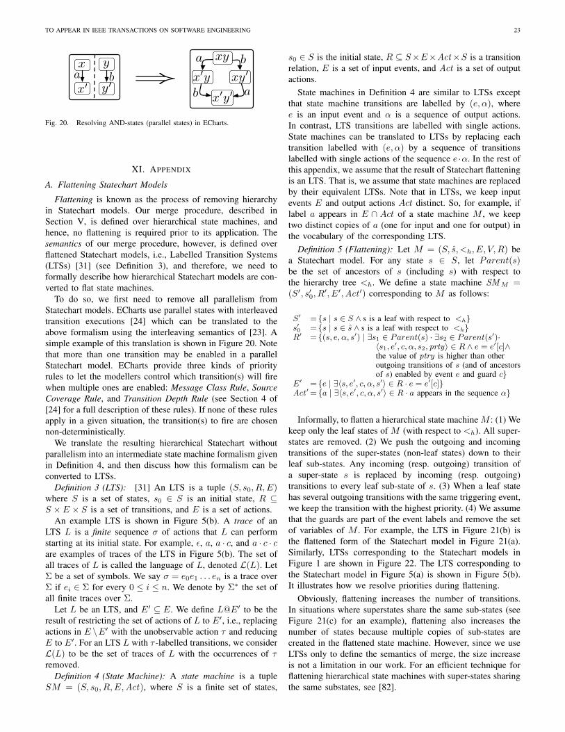
TO APPEAR IN IEEE TRANSACTIONS ON SOFTWARE ENGINEERING 23
x′
x y
y′a b
xy
x′y
x′y′
xy′a b
b⇒
a
Fig. 20. Resolving AND-states (parallel states) in ECharts.
XI. APPENDIX
A. Flattening Statechart Models
Flattening is known as the process of removing hierarchyin Statechart models. Our merge procedure, described inSection V, is defined over hierarchical state machines, andhence, no flattening is required prior to its application. Thesemantics of our merge procedure, however, is defined overflattened Statechart models, i.e., Labelled Transition Systems(LTSs) [31] (see Definition 3), and therefore, we need toformally describe how hierarchical Statechart models are con-verted to flat state machines.
To do so, we first need to remove all parallelism fromStatechart models. ECharts use parallel states with interleavedtransition executions [24] which can be translated to theabove formalism using the interleaving semantics of [23]. Asimple example of this translation is shown in Figure 20. Notethat more than one transition may be enabled in a parallelStatechart model. ECharts provide three kinds of priorityrules to let the modellers control which transition(s) will firewhen multiple ones are enabled: Message Class Rule, SourceCoverage Rule, and Transition Depth Rule (see Section 4 of[24] for a full description of these rules). If none of these rulesapply in a given situation, the transition(s) to fire are chosennon-deterministically.
We translate the resulting hierarchical Statechart withoutparallelism into an intermediate state machine formalism givenin Definition 4, and then discuss how this formalism can beconverted to LTSs.
Definition 3 (LTS): [31] An LTS is a tuple (S, s0, R,E)where S is a set of states, s0 ∈ S is an initial state, R ⊆S × E × S is a set of transitions, and E is a set of actions.
An example LTS is shown in Figure 5(b). A trace of anLTS L is a finite sequence σ of actions that L can performstarting at its initial state. For example, ε, a, a · c, and a · c · care examples of traces of the LTS in Figure 5(b). The set ofall traces of L is called the language of L, denoted L(L). LetΣ be a set of symbols. We say σ = e0e1 . . . en is a trace overΣ if ei ∈ Σ for every 0 ≤ i ≤ n. We denote by Σ∗ the set ofall finite traces over Σ.
Let L be an LTS, and E′ ⊆ E. We define L@E′ to be theresult of restricting the set of actions of L to E′, i.e., replacingactions in E \E′ with the unobservable action τ and reducingE to E′. For an LTS L with τ -labelled transitions, we considerL(L) to be the set of traces of L with the occurrences of τremoved.
Definition 4 (State Machine): A state machine is a tupleSM = (S, s0, R,E,Act), where S is a finite set of states,
s0 ∈ S is the initial state, R ⊆ S×E×Act×S is a transitionrelation, E is a set of input events, and Act is a set of outputactions.
State machines in Definition 4 are similar to LTSs exceptthat state machine transitions are labelled by (e, α), wheree is an input event and α is a sequence of output actions.In contrast, LTS transitions are labelled with single actions.State machines can be translated to LTSs by replacing eachtransition labelled with (e, α) by a sequence of transitionslabelled with single actions of the sequence e ·α. In the rest ofthis appendix, we assume that the result of Statechart flatteningis an LTS. That is, we assume that state machines are replacedby their equivalent LTSs. Note that in LTSs, we keep inputevents E and output actions Act distinct. So, for example, iflabel a appears in E ∩ Act of a state machine M , we keeptwo distinct copies of a (one for input and one for output) inthe vocabulary of the corresponding LTS.
Definition 5 (Flattening): Let M = (S, s, <h, E, V,R) bea Statechart model. For any state s ∈ S, let Parent(s)be the set of ancestors of s (including s) with respect tothe hierarchy tree <h. We define a state machine SMM =(S′, s′0, R
′, E′,Act ′) corresponding to M as follows:
S′ = {s | s ∈ S ∧ s is a leaf with respect to <h}s′0 = {s | s ∈ s ∧ s is a leaf with respect to <h}R′ = {(s, e, α, s′) | ∃s1 ∈ Parent(s) · ∃s2 ∈ Parent(s′)·
〈s1, e′, c, α, s2, prty〉 ∈ R ∧ e = e′[c]∧the value of ptry is higher than otheroutgoing transitions of s (and of ancestorsof s) enabled by event e and guard c}
E′ = {e | ∃〈s, e′, c, α, s′〉 ∈ R · e = e′[c]}Act ′= {a | ∃〈s, e′, c, α, s′〉 ∈ R · a appears in the sequence α}
Informally, to flatten a hierarchical state machine M : (1) Wekeep only the leaf states of M (with respect to <h). All super-states are removed. (2) We push the outgoing and incomingtransitions of the super-states (non-leaf states) down to theirleaf sub-states. Any incoming (resp. outgoing) transition ofa super-state s is replaced by incoming (resp. outgoing)transitions to every leaf sub-state of s. (3) When a leaf statehas several outgoing transitions with the same triggering event,we keep the transition with the highest priority. (4) We assumethat the guards are part of the event labels and remove the setof variables of M . For example, the LTS in Figure 21(b) isthe flattened form of the Statechart model in Figure 21(a).Similarly, LTSs corresponding to the Statechart models inFigure 1 are shown in Figure 22. The LTS corresponding tothe Statechart model in Figure 5(a) is shown in Figure 5(b).It illustrates how we resolve priorities during flattening.
Obviously, flattening increases the number of transitions.In situations where superstates share the same sub-states (seeFigure 21(c) for an example), flattening also increases thenumber of states because multiple copies of sub-states arecreated in the flattened state machine. However, since we useLTSs only to define the semantics of merge, the size increaseis not a limitation in our work. For an efficient technique forflattening hierarchical state machines with super-states sharingthe same substates, see [82].
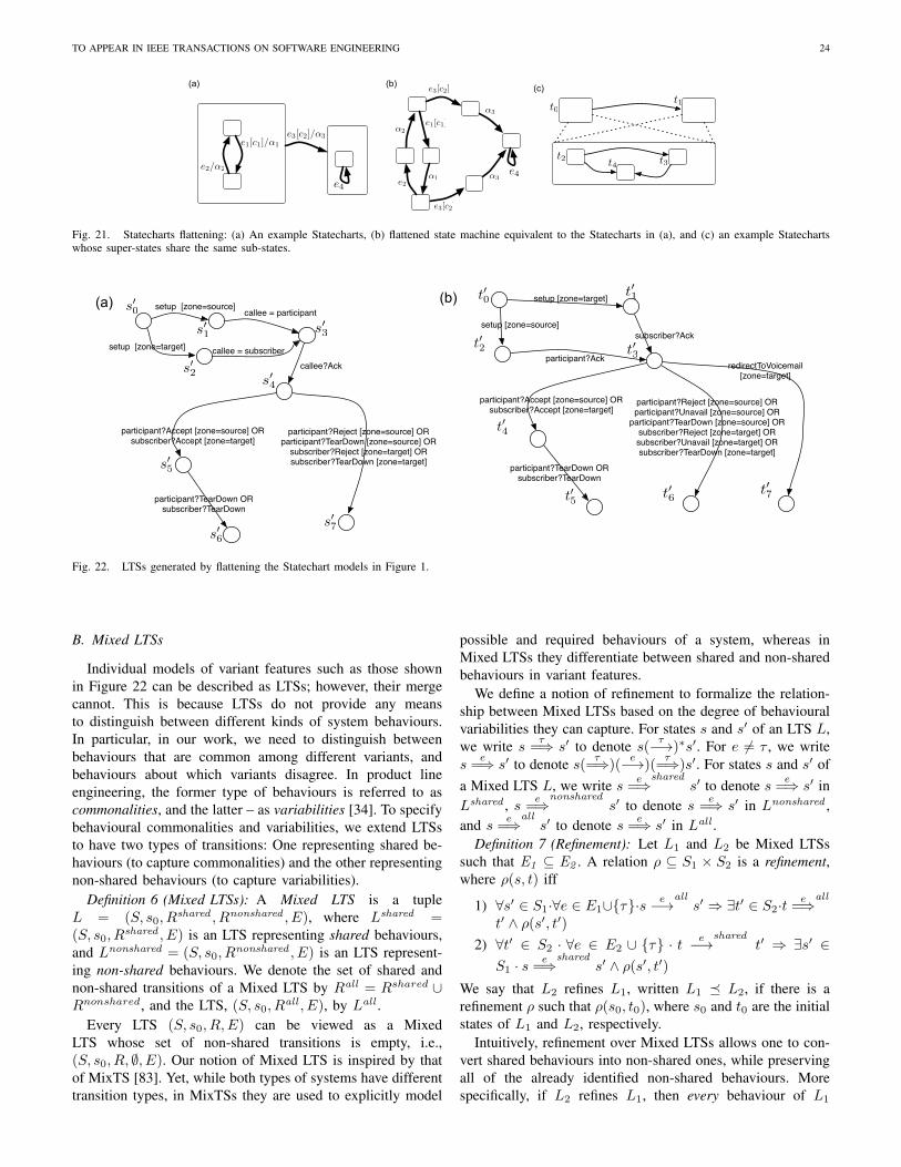
TO APPEAR IN IEEE TRANSACTIONS ON SOFTWARE ENGINEERING 24
e1[c1]/α1
e2/α2
e3[c2]/α3
e4
(a) (b) (c)
t0t1
t2 t3t4
e1[c1]
α1e2
α2
e3[c2]
α3e4
e3[c2]
α3
Fig. 21. Statecharts flattening: (a) An example Statecharts, (b) flattened state machine equivalent to the Statecharts in (a), and (c) an example Statechartswhose super-states share the same sub-states.
setup [zone=source]
callee?Ack
participant?Reject [zone=source] ORparticipant?TearDown [zone=source] OR
subscriber?Reject [zone=target] ORsubscriber?TearDown [zone=target]
participant?TearDown ORsubscriber?TearDown
participant?Accept [zone=source] ORsubscriber?Accept [zone=target]
setup [zone=target]
setup [zone=target]
setup [zone=source]
participant?Ack
subscriber?Ack
redirectToVoicemail[zone=target]
participant?Reject [zone=source] ORparticipant?Unavail [zone=source] OR
participant?TearDown [zone=source] ORsubscriber?Reject [zone=target] ORsubscriber?Unavail [zone=target] ORsubscriber?TearDown [zone=target]
participant?TearDown ORsubscriber?TearDown
participant?Accept [zone=source] ORsubscriber?Accept [zone=target]
s′0
s′1
s′2
s′3
s′4
s′5
(a) t′0 t′1
t′2 t′3
t′4
t′5 t′6 t′7
(b)
callee = subscriber
callee = participant
s′6
s′7
Fig. 22. LTSs generated by flattening the Statechart models in Figure 1.
B. Mixed LTSs
Individual models of variant features such as those shownin Figure 22 can be described as LTSs; however, their mergecannot. This is because LTSs do not provide any meansto distinguish between different kinds of system behaviours.In particular, in our work, we need to distinguish betweenbehaviours that are common among different variants, andbehaviours about which variants disagree. In product lineengineering, the former type of behaviours is referred to ascommonalities, and the latter – as variabilities [34]. To specifybehavioural commonalities and variabilities, we extend LTSsto have two types of transitions: One representing shared be-haviours (to capture commonalities) and the other representingnon-shared behaviours (to capture variabilities).
Definition 6 (Mixed LTSs): A Mixed LTS is a tupleL = (S, s0, R
shared , Rnonshared , E), where Lshared =(S, s0, R
shared , E) is an LTS representing shared behaviours,and Lnonshared = (S, s0, R
nonshared , E) is an LTS represent-ing non-shared behaviours. We denote the set of shared andnon-shared transitions of a Mixed LTS by Rall = Rshared ∪Rnonshared, and the LTS, (S, s0, R
all , E), by Lall .Every LTS (S, s0, R,E) can be viewed as a Mixed
LTS whose set of non-shared transitions is empty, i.e.,(S, s0, R, ∅, E). Our notion of Mixed LTS is inspired by thatof MixTS [83]. Yet, while both types of systems have differenttransition types, in MixTSs they are used to explicitly model
possible and required behaviours of a system, whereas inMixed LTSs they differentiate between shared and non-sharedbehaviours in variant features.
We define a notion of refinement to formalize the relation-ship between Mixed LTSs based on the degree of behaviouralvariabilities they can capture. For states s and s′ of an LTS L,we write s τ
=⇒ s′ to denote s( τ−→)∗s′. For e 6= τ , we writes
e=⇒ s′ to denote s( τ
=⇒)(e−→)(
τ=⇒)s′. For states s and s′ of
a Mixed LTS L, we write s e=⇒shared
s′ to denote s e=⇒ s′ in
Lshared , s e=⇒nonshared
s′ to denote s e=⇒ s′ in Lnonshared ,
and s e=⇒all
s′ to denote s e=⇒ s′ in Lall .
Definition 7 (Refinement): Let L1 and L2 be Mixed LTSssuch that E1 ⊆ E2 . A relation ρ ⊆ S1 × S2 is a refinement,where ρ(s, t) iff
1) ∀s′ ∈ S1·∀e ∈ E1∪{τ}·s e−→alls′ ⇒ ∃t′ ∈ S2·t e
=⇒all
t′ ∧ ρ(s′, t′)
2) ∀t′ ∈ S2 · ∀e ∈ E2 ∪ {τ} · t e−→sharedt′ ⇒ ∃s′ ∈
S1 · s e=⇒shared
s′ ∧ ρ(s′, t′)
We say that L2 refines L1, written L1 � L2, if there is arefinement ρ such that ρ(s0, t0), where s0 and t0 are the initialstates of L1 and L2, respectively.
Intuitively, refinement over Mixed LTSs allows one to con-vert shared behaviours into non-shared ones, while preservingall of the already identified non-shared behaviours. Morespecifically, if L2 refines L1, then every behaviour of L1
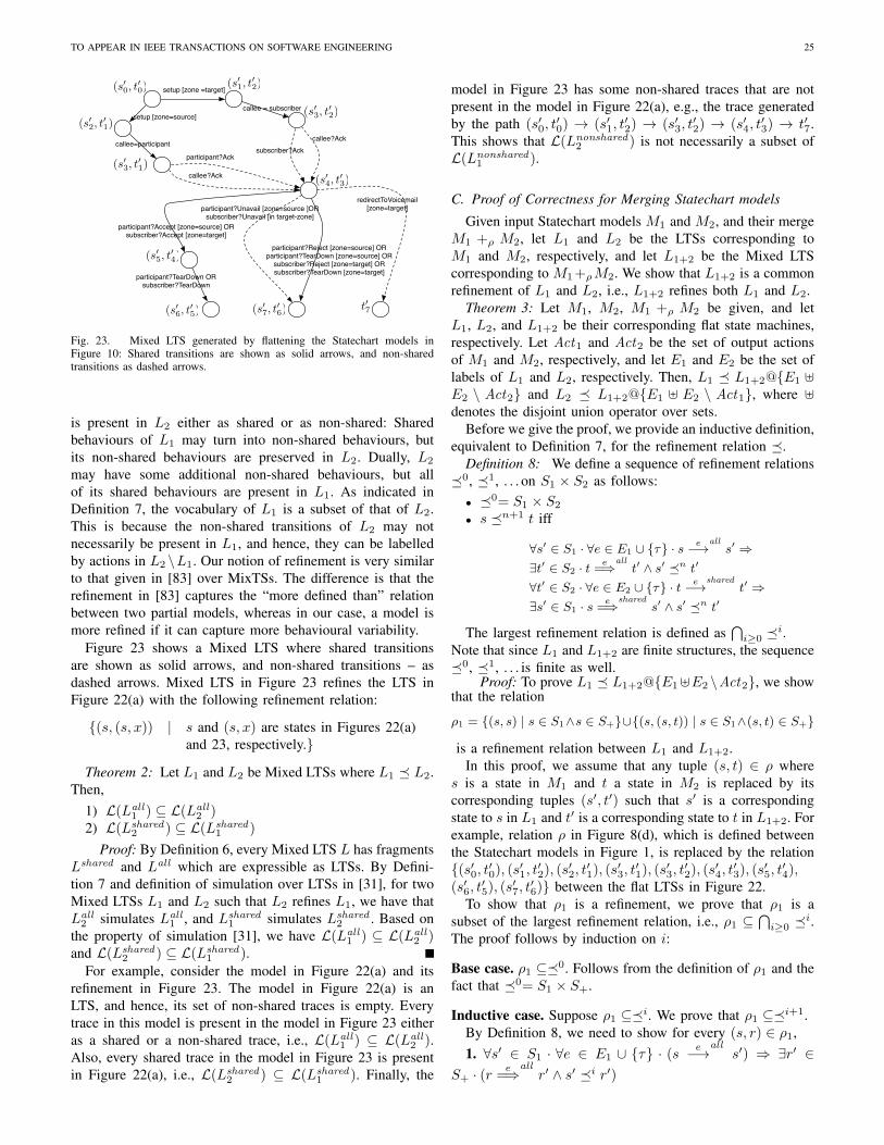
TO APPEAR IN IEEE TRANSACTIONS ON SOFTWARE ENGINEERING 25
setup [zone =target]
setup [zone=source]
participant?Ack subscriber?Ack
redirectToVoicemail[zone=target]
participant?Reject [zone=source] ORparticipant?TearDown [zone=source] OR
subscriber?Reject [zone=target] ORsubscriber?TearDown [zone=target]participant?TearDown OR
subscriber?TearDown
participant?Accept [zone=source] ORsubscriber?Accept [zone=target]
callee?Ack
callee?Ack
callee = subscriber
callee=participant
participant?Unavail [zone=source ]ORsubscriber?Unavail [in target-zone]
(s′0, t
′0)
(s′2, t
′1)
(s′1, t
′2)
(s′3, t
′1)
(s′3, t
′2)
(s′4, t
′3)
(s′5, t
′4)
(s′6, t
′5) (s′
7, t′6) t′7
Fig. 23. Mixed LTS generated by flattening the Statechart models inFigure 10: Shared transitions are shown as solid arrows, and non-sharedtransitions as dashed arrows.
is present in L2 either as shared or as non-shared: Sharedbehaviours of L1 may turn into non-shared behaviours, butits non-shared behaviours are preserved in L2. Dually, L2
may have some additional non-shared behaviours, but allof its shared behaviours are present in L1. As indicated inDefinition 7, the vocabulary of L1 is a subset of that of L2.This is because the non-shared transitions of L2 may notnecessarily be present in L1, and hence, they can be labelledby actions in L2 \L1. Our notion of refinement is very similarto that given in [83] over MixTSs. The difference is that therefinement in [83] captures the “more defined than” relationbetween two partial models, whereas in our case, a model ismore refined if it can capture more behavioural variability.
Figure 23 shows a Mixed LTS where shared transitionsare shown as solid arrows, and non-shared transitions – asdashed arrows. Mixed LTS in Figure 23 refines the LTS inFigure 22(a) with the following refinement relation:
{(s, (s, x)) | s and (s, x) are states in Figures 22(a)and 23, respectively.}
Theorem 2: Let L1 and L2 be Mixed LTSs where L1 � L2.Then,
1) L(Lall1 ) ⊆ L(Lall
2 )2) L(Lshared
2 ) ⊆ L(Lshared1 )
Proof: By Definition 6, every Mixed LTS L has fragmentsLshared and Lall which are expressible as LTSs. By Defini-tion 7 and definition of simulation over LTSs in [31], for twoMixed LTSs L1 and L2 such that L2 refines L1, we have thatLall2 simulates Lall
1 , and Lshared1 simulates Lshared
2 . Based onthe property of simulation [31], we have L(Lall
1 ) ⊆ L(Lall2 )
and L(Lshared2 ) ⊆ L(Lshared
1 ).For example, consider the model in Figure 22(a) and its
refinement in Figure 23. The model in Figure 22(a) is anLTS, and hence, its set of non-shared traces is empty. Everytrace in this model is present in the model in Figure 23 eitheras a shared or a non-shared trace, i.e., L(Lall
1 ) ⊆ L(Lall2 ).
Also, every shared trace in the model in Figure 23 is presentin Figure 22(a), i.e., L(Lshared
2 ) ⊆ L(Lshared1 ). Finally, the
model in Figure 23 has some non-shared traces that are notpresent in the model in Figure 22(a), e.g., the trace generatedby the path (s′0, t
′0) → (s′1, t
′2) → (s′3, t
′2) → (s′4, t
′3) → t′7.
This shows that L(Lnonshared2 ) is not necessarily a subset of
L(Lnonshared1 ).
C. Proof of Correctness for Merging Statechart models
Given input Statechart models M1 and M2, and their mergeM1 +ρ M2, let L1 and L2 be the LTSs corresponding toM1 and M2, respectively, and let L1+2 be the Mixed LTScorresponding to M1+ρM2. We show that L1+2 is a commonrefinement of L1 and L2, i.e., L1+2 refines both L1 and L2.
Theorem 3: Let M1, M2, M1 +ρ M2 be given, and letL1, L2, and L1+2 be their corresponding flat state machines,respectively. Let Act1 and Act2 be the set of output actionsof M1 and M2, respectively, and let E1 and E2 be the set oflabels of L1 and L2, respectively. Then, L1 � L1+2@{E1 ]E2 \ Act2} and L2 � L1+2@{E1 ] E2 \ Act1}, where ]denotes the disjoint union operator over sets.
Before we give the proof, we provide an inductive definition,equivalent to Definition 7, for the refinement relation �.
Definition 8: We define a sequence of refinement relations�0, �1, . . . on S1 × S2 as follows:• �0= S1 × S2
• s �n+1 t iff
∀s′ ∈ S1 · ∀e ∈ E1 ∪ {τ} · se−→
alls′ ⇒
∃t′ ∈ S2 · te
=⇒allt′ ∧ s′ �n t′
∀t′ ∈ S2 · ∀e ∈ E2 ∪ {τ} · te−→
sharedt′ ⇒
∃s′ ∈ S1 · se
=⇒shared
s′ ∧ s′ �n t′
The largest refinement relation is defined as⋂i≥0 �i.
Note that since L1 and L1+2 are finite structures, the sequence�0, �1, . . . is finite as well.
Proof: To prove L1 � L1+2@{E1]E2 \Act2}, we showthat the relation
ρ1 = {(s, s) | s ∈ S1∧s ∈ S+}∪{(s, (s, t)) | s ∈ S1∧(s, t) ∈ S+}
is a refinement relation between L1 and L1+2.In this proof, we assume that any tuple (s, t) ∈ ρ where
s is a state in M1 and t a state in M2 is replaced by itscorresponding tuples (s′, t′) such that s′ is a correspondingstate to s in L1 and t′ is a corresponding state to t in L1+2. Forexample, relation ρ in Figure 8(d), which is defined betweenthe Statechart models in Figure 1, is replaced by the relation{(s′0, t′0), (s′1, t
′2), (s′2, t
′1), (s′3, t
′1), (s′3, t
′2), (s′4, t
′3), (s′5, t
′4),
(s′6, t′5), (s′7, t
′6)} between the flat LTSs in Figure 22.
To show that ρ1 is a refinement, we prove that ρ1 is asubset of the largest refinement relation, i.e., ρ1 ⊆
⋂i≥0 �i.
The proof follows by induction on i:
Base case. ρ1 ⊆�0. Follows from the definition of ρ1 and thefact that �0= S1 × S+.
Inductive case. Suppose ρ1 ⊆�i. We prove that ρ1 ⊆�i+1.By Definition 8, we need to show for every (s, r) ∈ ρ1,1. ∀s′ ∈ S1 · ∀e ∈ E1 ∪ {τ} · (s
e−→alls′) ⇒ ∃r′ ∈
S+ · (r e=⇒all
r′ ∧ s′ �i r′)
TO APPEAR IN IEEE TRANSACTIONS ON SOFTWARE ENGINEERING 26
2. ∀r′ ∈ S+ · ∀e ∈ (E1 ] E2 ∪ {τ}) \ Act2 · (r e−→shared
r′)⇒ ∃s′ ∈ S1 · (s e=⇒shared
s′ ∧ s′ �i r′)To prove 1., we identify four cases:
Case 1: ∀s′ ∈ S1 · ∀e ∈ E1 ∪ {τ} · se−→
alls′∧
∃t, t′ ∈ S2 · (s, t) ∈ ρ ∧ (s′, t′) ∈ ρ⇒ (by construction of M1 +ρM2 in Section V-B and
definition of ρ1)r = (s, t) ∧ ∃(s′, t′) ∈ S+ · (s, t)
e−→all
(s′, t′)∧(s′, (s′, t′)) ∈ ρ1
⇒ (by the inductive hypothesis, and let r′ = (s′, t′))∃r′ ∈ S+ · r
e−→allr′ ∧ s′ �i r′
Case 2: ∀s′ ∈ S1 · ∀e ∈ E1 ∪ {τ} · se−→
alls′∧
∃t ∈ S2 · (s, t) ∈ ρ∧ 6 ∃t′ ∈ S2 · (s′, t′) ∈ ρ⇒ (by construction of M1 +ρM2 in Section V-B)
r = (s, t)∧ 6 ∃t′ ∈ S2 · (s′, t′) ∈ ρ ∧ (s, t)e−→
alls′
⇒ (by definition of S+ and ρ1)∃t ∈ S2 · r = (s, t) ∧ ∃s′ ∈ S+ · (s, t)
e−→alls′∧
(s′, s′) ∈ ρ1⇒ (by the inductive hypothesis, and let r′ = s′)
∃r′ ∈ S+ · re−→
allr′ ∧ s′ �i r′
Case 3: ∀s′ ∈ S1 · ∀e ∈ E1 ∪ {τ} · se−→
alls′∧
6 ∃t ∈ S2 · (s, t) ∈ ρ ∧ ∃t′ ∈ S2 · (s′, t′) ∈ ρ⇒ (by construction of M1 +ρM2 in Section V-B)
r = s ∧ ∃t′ ∈ S2 · (s′, t′) ∈ ρ ∧ se−→
all(s′, t′)
⇒ (by definition of S+ and ρ1)∃(s′, t′) ∈ S+ · s
e−→all
(s′, t′) ∧ (s′, (s′, t′)) ∈ ρ1⇒ (by the inductive hypothesis, and let r′ = (s′, t′))
∃r′ ∈ S+ · re−→
allr′ ∧ s′ �i (s′, t′)
Case 4: ∀s′ ∈ S1 · ∀e ∈ E1 ∪ {τ} · se−→
alls′∧
6 ∃t ∈ S2 · (s, t) ∈ ρ∧ 6 ∃t′ ∈ S2 · (s′, t′) ∈ ρ⇒ (by construction of M1 +ρM2 in Section V-B)
r = s∧ 6 ∃t′ ∈ S2 · (s′, t′) ∈ ρ ∧ se−→
alls′
⇒ (by definition of S+ and ρ1)∃s′ ∈ S+ · s
e−→alls′ ∧ (s′, s′) ∈ ρ1
⇒ (by the inductive hypothesis, and let r′ = s′)∃r′ ∈ S+ · r
e−→allr′ ∧ s′ �i r′
To prove 2., by construction of merge in Section V-B, forany shared transition r e−→shared
r′ in L1+2, we have• if e 6= τ , then ∃(s, t), (s′, t′) ∈ ρ·r = (s, t)∧r′ = (s′, t′).• if e = τ , then ∃(s, t), (s, t′) ∈ ρ · r = (s, t)∧ r′ = (s, t′).
∀r′ ∈ S+ · ∀e ∈ (E1 ] E2) \Act2 · re−→
sharedr′∧(
∃(s, t), (s′, t′) ∈ ρ · r = (s, t) ∧ r′ = (s′, t′) ∧ e 6= τ∨
∃(s, t), (s, t′) ∈ ρ · r = (s, t) ∧ r′ = (s, t′) ∧ e = τ)
⇒ (by construction of M1 +ρM2 in Section V-B)∃(s, t), (s′, t′) ∈ ρ · r = (s, t) ∧ r′ = (s′, t′)∧s
e−→shared
s′ ∧ e 6= τ∨
∃(s, t), (s, t′) ∈ ρ · r = (s, t) ∧ r′ = (s, t′)∧s
e=⇒
shareds ∧ e = τ
⇒ (by definition of ρ and ρ1)∃s′ ∈ S1 · s
e−→shared
s′ ∧ (s′, (s′, t′)) ∈ ρ1 ∧ e 6= τ∨
sτ
=⇒shared
s ∧ (s, (s, t′)) ∈ ρ1⇒ (by the inductive hypothesis)
∃s′ ∈ S1 · se
=⇒shared
s′ ∧ s′ �i r′
The above proves that ρ1 ⊆⋂i≥0 �i. Since ρ1 also relates
s0 (the initial state of L1) to (s0, t0) (the initial state of L1+2),ρ1 is indeed a refinement relation between L1 and L1+2. ρ1might not be the largest refinement relation, but any refinementrelation that includes the initial states of its underlying modelscan preserve their temporal properties.
To prove L2 � L1+2, we show that the relation
σ2 = {(t, t) | t ∈ S+∧t ∈ S2}∪{(t, (s, t)) | t ∈ S2∧(s, t) ∈ S+}is a refinement relation between L2 and L1+2. The proof issymmetric to the one above.
Recall that by our definition in Section V-B, shared tran-sitions r and r′ must have identical events, conditions, andpriorities, but they may generate different output actions. Thereason that we do not require actions of shared transitions tobe identical is that by our assumption in Section III, the inputStatechart models are non-interacting, and hence, actions inone input model do not trigger any event in the other model.In our merge procedure, for any pair of shared transitions rand r′, we create a single transition r′′ in the merge that canproduce the union of the actions of r and r′. Thus, the tracegenerated by r′′ may not exactly match the traces of r andr′. For example, consider the following shared transitions inFigure 1:
s2setup[zone=target]/callee==subscriber−−−−−−−−−−−−−−−−−−−−−−−−−→ s3 and
t1setup[zone=target]−−−−−−−−−−−−→ t3
These transitions are lifted to the transition
(s2, t1)setup[zone=target]/callee==subscriber−−−−−−−−−−−−−−−−−−−−−−−−−→ (s3, t3)
in the merge in Figure 10, but the action callee==subscriberdoes not exist in Figure 1(b). Thus, we need to hide thisaction when comparing the merge with the model in Fig-ure 1(b). Figure 24 shows the Mixed LTS correspondingto the merge in Figure 10 where actions callee==subscriberand callee==participant are hidden. It can be seen that thisMixed LTS is a refinement of the LTS corresponding tothe model in Figure 1(b) where the refinement relationis {((s, t), t) | (s, t) and t are states in Figure 10 and 1(b),respectively. }.
By Theorems 2 and 3, we have(1) L(Lshared
1+2 @{E1 ] E2 \ Act2}) ⊆ L(Lall1 ), and
L(Lshared1+2 @{E1 ] E2 \ Act1}) ⊆ L(Lall
2 ). That is,the set of shared, i.e., unguarded, behaviours of themerge is a subset of the behaviours of the individualinput models.
(2) L(Lall1 ) ⊆ L(Lall
1+2), and L(Lall2 ) ⊆ L(Lall
1+2). Thatis, behaviours of the individual input models arepresent as either shared, i.e., unguarded, or non-shared, i.e., guarded, behaviours in their merge.
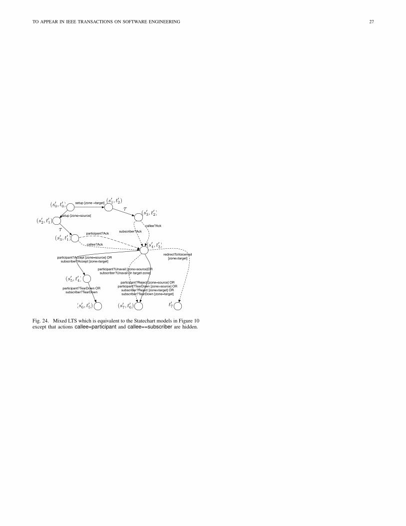
TO APPEAR IN IEEE TRANSACTIONS ON SOFTWARE ENGINEERING 27
setup [zone =target]
setup [zone=source]
participant?Ack subscriber?Ack
redirectToVoicemail[zone=target]
participant?Reject [zone=source] ORparticipant?TearDown [zone=source] OR
subscriber?Reject [zone=target] ORsubscriber?TearDown [zone=target]
participant?TearDown ORsubscriber?TearDown
participant?Accept [zone=source] ORsubscriber?Accept [zone=target]
callee?Ack
callee?Ack
τ
τ
participant?Unavail [zone=source]ORsubscriber?Unavail [in target-zone]
(s′0, t
′0)
(s′2, t
′1)
(s′1, t
′2)
(s′3, t
′1)
(s′3, t
′2)
(s′4, t
′3)
(s′5, t
′4)
(s′6, t
′5) (s′
7, t′6) t′7
Fig. 24. Mixed LTS which is equivalent to the Statechart models in Figure 10except that actions callee=participant and callee==subscriber are hidden.