ARMY

TM5-852-6AIR FORCE AFR 88-19, Volume 6

TECHNICAL MANUAL

ARCTIC AND SUBARCTICCONSTRUCTION

CALCULATION METHODSFOR DETERMINATION OFDEPTHS OF FREEZE AND

THAW IN SOILS

DEPARTMENTS OF THE ARMY AND THE AIR FORCE

JANUARY 1988

REPRODUCTION AUTHORIZATION/RESTRICTIONSThis manual has been prepared by or for the Government and is public property

and not subject to copyright .Reprints or republications ofthis manual should include a credit line substantially

as follows : "Joint Departments of the Army and Air Force USA, Technical ManualTM 5-852-6/AFR 88-19, Volume 6, Calculation Methods for Determination of Depthsof Freeze and Thaw in soils, date."

TECHNICALMANUAL

HEADQUARTERSNO. 5-852-6

DEPARTMENTSOF THE ARMYAIR FORCE REGULATION

ANDTHE AIRFORCEAFR 88-19, VOLUME 6

WASHINGTON, DC, 25 January 1988

ARCTIC AND SUBARCTIC CONSTRUCTION-CALCULATION METHODS FORDETERMINATION OF DEPTHS OF FREEZE ANDTHAW IN SOILS

"This manual supercedes TM 5-852-6/AFM 88-19, Chap . 6, dated January 1966 .

Paragraph PageCHAPTER 1. GENERAL

Purpose and scope . . . . . . . . . . . . . . . . . . . . . . . . . . . . . . . . . . . . . . 1-1 1-1References and symbols . . . . . . . . . . . . . . . . . . . . . . . . . . . . . . . . 1-2 1-1Background . . . . . . . . . . . . . . . . . . . . . . . . . . . . . . . . . . . . . . . . . . . . 1-3 1-1

CHAPTER 2. DEFINITIONS AND THERMALPROPERTIES

Definitions 2-1 2-1Thermal properties of soilsand other constructionmaterials . . . . . . . . . . . . . . . . . . . . . . . . . . . . . . . . . . . . . . . . . . . . . . . 2-2 2-2Fundamental considerations . . . . . . . . . . . . . . . . . . . . . . . . . . . 2-3 2-3Freezing and thawingindexes . . . . . . . . . . . . . . . . . . . . . . . . . . . . . . . . . . . . . . . . . . . . . . . . 2-4 2-5

CHAPTER 3. ONE-DIMENSIONAL LINEARANDPERIODIC MEAT FLOW

Thermal regime . . . . . . . . . . . . . . . . . . . . . . . . . . . . . . . . . . . . . . . . . 3-1 3-1Modified Berggren equation . . . . . . . . . . . . . . . . . . . . . . . . . . . . 3-2 3-1Homogeneous soils . . . . . . . . . . . . . . . . . . . . . . . . . . . . . . . . . . . . . 3-3 3-3Multilayer soils . . . . . . . . . . . . . . . . . . . . . . . . . . . . . . . . . . . . . . . . . 3-4 3-3Effect of snow andvegetative cover . . . . . . . . . . . . . . . . . . . . : . . . . . . . . . . . . . . . . . . . 3-5 3-6Surface temperaturevariations . . . . . . . . . . . . . . . . . . . . . . . . . . . . . . . . . . . . . . . . . . . . . . 3-6 3-6Converting indexes intoequivalent sine waves oftemperature . . . . . . . . . . . . . . . . . . . . . . . . . . . . . . . . . . . . . . . . . . . 3-7 3-8Penetration of freeze orthaw beneath buildings . . . . . . . . . . . . . . . . . . . . . . . . . . . . . . . . 3-8 3-11Use of thermal insulatingmaterials . . . . . . . . . . . . . . . . . . . . . . . . . . . . . . . . . . . . . . . . . . . . 3-9 3-18

CHAPTER 4. TWO-DIMENSIONAL RADIAL HEATFLOW

General . . . . . . . . . . . . . . . . . . . . . . . . . . . . . . . . . . . . . . . . . . . . . . . . . . . . . . . . . . . . . 4-1 4-1Pile installation inpermafrost . . . . . . . . . . . . . . . . . . . . . . . . . . . . . . . . . . . . . . . . . . . . . . . . . . . . . . . . 4-2 4-2Utility distribution systemsin frozen ground . . . . . . . . . . . . . . . . . . . . . . . . . . . . . . . . . . . . . . . . . . . . . . . . . 4-3 4-7Discussion of multi-dimensional heat flow . . . . . . . . . . . . . . . . . . . . . . . . . . . . . . . . . . . . . . . . . 4-4 4-13

APPENDIX A. LIST OF SYMBOLS A-1APPENDIX B. THERMALMODELS FORCOMPUTING

FREEZE ANDTHAWDEPTHS B-1APPENDIX C. REFERENCES C-1BIBLIOGRAPHY BIBLIO-1

Figure 2-1 . Average thermal conductivity for sands and gravels, frozen. . . . . . . . . . . . . . . . . . . . . . . . . . . . .

2-32-2. Average thermal conductivity for sands and gravels, unfrozen. . . . . . . . . . . . . . . . . . . . . . . . .

2.42-3. Average thermal conductivity for silt and clay soils, frozen . . . . . . . . . . . . . . . . . . . . . . . . . . . . . .

2.42-4. Average thermal conductivity for silt and clay soils, unfrozen. . . . . . . . . . . . . . . . . . . . . . . . . .

2.42-5. Average thermal conductivity for peat, frozen. . . . . . . . . . . . . . . . . . . . . . . . . . . . . . . . . . . . . . . . . . . . . .

2.52-6. Average thermal conductivity for peat, unfrozen. . . . . . . . . . . . . . . . . . . . . . . . . . . . . . . . . . . . . . . . . . .

2.52-7. Average volumetric heat capacity for soils . . . . . . . . . . . . . . . . . . . . . . . . . . . . . . . . . . . . . . . . . . . . . . . . . . .

2.82-8.7dolumetriclatentheatforsoils . . . . . . . . . . . . . . . . . . . . . . . . . . . . . . . . . . . . . . . . . . . . . . � .�������� 2.92-9. Average monthly temperatures versus time at Fairbanks, Alaska- . . . . . . . . . . . . . . . . . . . . . 2-102-10Relationship between wind speed and n-factor during thawing season. . . . . . . . . . . . . . . . 2-112-11 .Relationship between mean freezing index and maximum freezing index for

10 years of record, 1953-1962 (arctic and subarctic regions). . . . . . . . . . . . . . . . . . . . . . . . . . . . . . . 2-122-12Relationship between mean thawing index and maximum thawing index for

10 years of record, 1953-1962 (arctic and subarctic regions). . . . . . . . . . . . . . . . . . . . . . . . . . . . . . . 2-133-1 . .1 coefficient in modified Berggren formula.

3-23-2. Relationship between (x/2;att-) and erf (x/287_1)

. . . . . . . . . . . . .. . . . . . . . .. . . . . . . . . . . . . . . . . . . . . . . . . . . . .. . . . . . . . . . . . . . . . . . . . . . . . . . . . . . . . . . . . . . . . . . . .

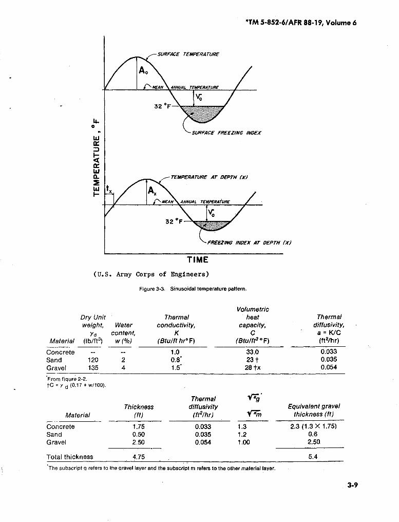
3-73-3. Sinusoidal temperature pattern . . . . . . . . . . . . . . . . . . . . . . . . . . . . . . . . . . . . . . . . . . . . . . . . . . . . . . . . . . . ., . . .

3.93-4. Indexes and equivalent sinusoidal temperature. . . . . . . . . . . . . . . . . . . . . . . . . . . . . . . . . . . . . . . . . . . . 3-103-5. Average monthly temperatures for 1949-1950 and equivalent sine wave,

Fairbanks, Alaska. . . . . . . . . . . . . . . . . . . . . . . . . . . . . . . . . . . . . . . . . . . . . . . . . . . . . . . . . . . . . . . . . . . . . . . . . . . . . . . . . . . 3-113-6. Long-term mean monthly temperatures and equivalent sine wave,

Fairbanks, Alaska. . . . . . . . . . . . . . . . . . . . . . . . . . . . . . . . . . . . . . . . . . . . . . . . . . . . . . . . . . . . . . . . . . . . . . . . . . . . . . . . . . 3-123-7. Schematic of ducted foundation . . . . . . . . . . , . . . . . . . . . . . . . . . . . . . . . . . . . . . . . . . . . . . . . . . . . � , . . . . . . 3-143-8. Properties of dry air at atmospheric pressure . . . . . . . . . . . . . . . . . . . . . . . . . . . . . . . . . . . . . . . . . . . . . . . 3-164-1 . Illustration for example in paragraph 4-la. . . . . . . . . . . . . . . . . . . . . . . . . . . . . . . . . . . . . . . . . . . . . . . . . . . . 4-24-2. Temperature around a cylinder having received a step change in temperature. . . . . 4-34-3. General solution of slurry freeze-back . . . . . . . . . . . . . . . . . . . . . . . . . . . . . . . . . . . . . . . . . . . . . . . . . . . . . . . .

4-44-4. Specific solution of slurry freeze-back. . . . . . . .. . . . . . . . . . . . . . . . . . . . . . . . . . . . . . . . . . . . . . . . . . . . . . . . .

4-54-5. Freezeup of stationary water in an uninsulated pipe. . . . . . . . . . . . . . . . . . . . . . . . . . . . . . . . . . . . . .

4-94-6. Temperature drop of flowing water in a pipeline. . . . . . . . . . . . . . . . . . . . . . . . . . . . . . . . . . . . . . . . . . . 4-12

Table

2-1. Specific heat values of various materials. . . . . . . . . . . . . . . . . . . . . . . . . . . . . . . . . . . . . . . . . . . . . . . . . . . . .

2.22-2. Thermal properties of construction materials . . . . . . . . . . . . . . . . . . . . . . . . . . . . . . . . . . . . . . . . . . . . . . .

2.62-3. Calculation of cumulative degree-days. . . . . . . . . . . . . . . . . . . . . . . . . . . . . . . . . . . . . . . .

. . . . . . . . . . . . . . .

2.92-4. n-factors for freeze and thaw. . . . . . . . . . . . . . . . . . . . . . . . . . . . . . . . . . . . . . . . . . . . . . . . . . . . . . . . . . . . . . . . . . . . . 2.113-1 . Multilayer solution of modified Berggren equation. . . . . . . . . . . . . . . . . . . . . . . . . . . . . . . . . . . . . . . .

3.53-2. Thaw penetration beneath a slab-on-grade building constructed

on permafrost. . . . . . . . . . . . . . . . . . . . . . . . . . . . . . . . . . . . . . . . . . . . . . . . . . . . . . . . . . . . . . . . . . . . . . . . . . . . . . . . . . . . . . . 3.133-3. Insulated pavement design, no frost penetration. . . . . . . . . . . . . . . . . . . . . . . . . . . . . . . . . . . . . . . . . . 3.203-4. Insulated pavement design, frost penetration. . . . . . . . . . . . . . . . . . . . . . . . . . . . . . . . . . . . . . . . . . . . . . 3.20B-1 . Thermal, fluid and electric analogs . . . . . . . . . . . . . . . . . . . . . . . . . . . . . . . . . . . . . . . . . . . . . . . . . . . . . . . . . . . .

B-2

LIST OF FIGURES

LIST OF TABLES

1-1 .

Purpose and scope .This manual contains criteria andmethods for calculating the depths offreeze andthawinsoils,with considera-tion of the effects of other adjacentmaterials, for the design of militaryfacilities in seasonal frost, arctic andsubaretic regions. The contents areapplicable to bothArmy and AirForceconstruction in arctic, subaretic andseasonal frost areas. The data pre-sented in this manual relate to arcticand subaretic facility design presentedin the other manuals of the Arctic andSubarctic Construction series .

1-2.

References and symbols .Appendix C lists the references forthis manual; appendix A contains a listof symbols.

1-3. Background.a. The depths to which soils may

freeze and thaw is very important inthe design of pavements, structuresand utilities in areas of seasonal frostandpermafrost. Methods ofcalculatingsuch depths, based on heat-transferprinciples, are presented here. Forderivation of basic equations, and the

CHAPTER 1

GENERAL

*TM 5-852-6/AFR 88-19, Volume 6

underlyingtheory, seeappendix Candthe bibliography .b. Heat transfer in soils involving

phase change of pore water is an ex-tremely complex process and manyproblems defy rigorous mathematicaltreatment. Themethods presentedhereare simplified procedures developedfor the solution of engineering designproblems.c. Several assumptions have been

made indeveloping practical methodsofcalculating depths of freeze or thawin soils . It is assumed that each layer ofmaterial is homogeneousand isotropic,and that the average thermal proper-ties of frozen and unfrozen soils areapplicable. Unless specific data areavailable, it is alsoassumed that all soilwater is converted to ice, or all ice isconverted to water, atatemperature of32°F. This latter assumption is sub-stantially correct for coarse-grainedsoils but only partially true for fine-grained soils.d. The services of the U.S. Army Cold

Regions Research and EngineeringLaboratory (USACRREL), Hanover,NewHampshire, are available to assist inthe development of solutions for heat-flow problems in soils.

2-1 . Definitions .Definitions of certain specialized terms

_ applicable to arctic and subarcticregions are contained in TM 5-8_5_2/AFR _S-1G,_Volume 1. Following areadditional terms used specifically inheat-transfer calculations .

a. Thermal conductivity, K. Thequantity of heat flow in a unit timethrough a unit area of a substancecaused by a unit thermal gradient.

b. Specific heat, c. The quantity ofheat absorbed (or given up) by a unitweight ofa substancewhen its temperature is increased (or decreased) by 1degree Fahrenheit (°F) divided by thequantity of heat absorbed (or given up)by a unit weight of water when itstemperature is increased (or decreased)by 1°F .

c. Volumetric heat capacity, C. Thequantity of heat required to changethe temperature of a unit volume by1°F.

Forunfrozen soils,

L=144 yd

CHAPTER 2

DEFINITIONS AND THERMAL PROPERTIES

WCu =yd(c+1.0

100Forfrozen soils,

WC f = yd (c + 0.5

100

)

(eq 2-2)

W

W

100

(eq 2-1)

Average values for most soils,

cavg. = Yd (c + 0.75

100

)

(eq 2-3)where c = specific heat ofthe soil solids(0.17 for most soils)

Yd = dry unit weight of soilw = water content of soil in per-

cent of dry weight .d. Volumetric latent heat offusion,

L. The quantity of heat required tomelt the ice (or freeze the water) in aunitvolume of soil withoutachange intemperature-in British thermal units(Btu) per cubic foot (ft3) :

(eq 2-4)

e. thermalresistance,R. The recipro-cal of the time rate ofheat flow througha unit area ofa soil layer of given thickness d per unit temperature difference :

f. Thermal diffusivity, a. An indica-tor ofhoweasily a material willundergotemperature change:

cg. Thermal ratio, a-

a

d

K

K

*TM 5-852-6/AFR 88-19, Volume 6

(eq 2-5)

(eq 2-6)

(eq 2-7)

wherevoabsolutevalue ofthe difference

' between the meanannual tem-perature below the groundsurface and 32°F.

vs one of two possible meanings,depending on the problembeing studied:

(1) vs = nF/t

(or nl/t)where

n=conversion factor from airindex to surface index

F= air freezing indexI =air thawing indext = length of freezing (or thawing)

season .(2) vs absolute value of the dif-

ference between the meanannualgroundsurface temp-erature and 32°F.

In the first case, vs is useful forcomputing the seasonal depthof freeze or thaw. In the secondcase, it is useful in computingmultiyear freeze or thawdepths that may develop as aresult of some long-termchange in the heat balance atthe ground surface.

h. Fusion parameter, /j"

*TM 5-852-6/AFR 88-19, Volume 6

C

2-2

N -_

"s

(eq2-8)L

whereve has the two possible meaningsnoted above.

i. "Lambda" coefficient, JI " A factorallowing for heat capacity and initialtemperature ofthe ground (see fig. 3-1).

Aadj).

(eq2-9)

j. Thermal regime. The temperaturepattern existing in a soil body in rela-tion to seasonal variations.

k. British thermal unit, Btu. Thequantity of heat required to raise thetemperature of1 pound (lb) ofwater 1°Fat about 40°F.

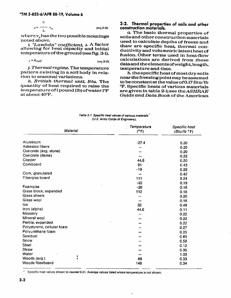
Table 2-1. Specific heat values of various materials .*(U.S. Army Corps of Engineers).

Specific heat values shown to nearest 0.01 . Average values listed where temperature is not shown .

2-2.

Thermal properties of soils and otherconstruction materials.

a. The basic thermal properties ofsoils and other construction materialsused to calculate depths of freeze andthaw are specific heat, thermal con-ductivity andvolumetric latent heat offusion. Other terms used in heat-flowcalculations are derived from thesedataand the elements ofweight, length,temperature and time.

b. the specific heat of most dry soilsnear the freezingpointmaybeassumedto be constantat the value of0.17 Btu/lb°F. Specific heats of various materialsare given in table 2-1 ; see theASFIRAEGuide and DataBook of the American

MaterialTemperature

(OF)Specific heat(Btullb OF)

Aluminum -27.4 0.20Asbestos fibers -- 0.25Concrete (avg . stone) -- 0.20Concrete (dams) - 0.22Copper 44.6 0.20Corkboard 91 0.43

-19 0.29Cork, granulated -- 0.42Fiberglas board 111 0.24

-22 0.19Foamglas -20 0.16Glass block, expanded 112 0.18Glass sheets -- 0.20Glass wool -- 0.16Ice 32 0.48Iron (alpha) 44.6 0.11Masonry __ 0.22Mineral wool __ 0.22Perlite, expanded __ 0.22Polystyrene, cellular foam __ 0.27Polyurethane foam -- 0.25Sawdust -- 0.60Snow -- 0.50Steel __ 0.12Straw -- 0.35Water -- 1 .00Woods (avg .) Y 68 0.33Woods fiberboard 148 0.34

Society of Heating and Air Condition-ing Engineers for the specific heatvalues ofcommon materials .

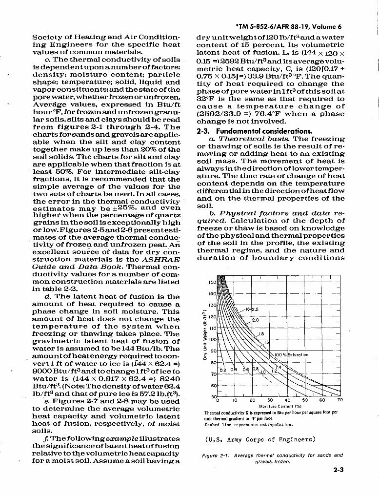
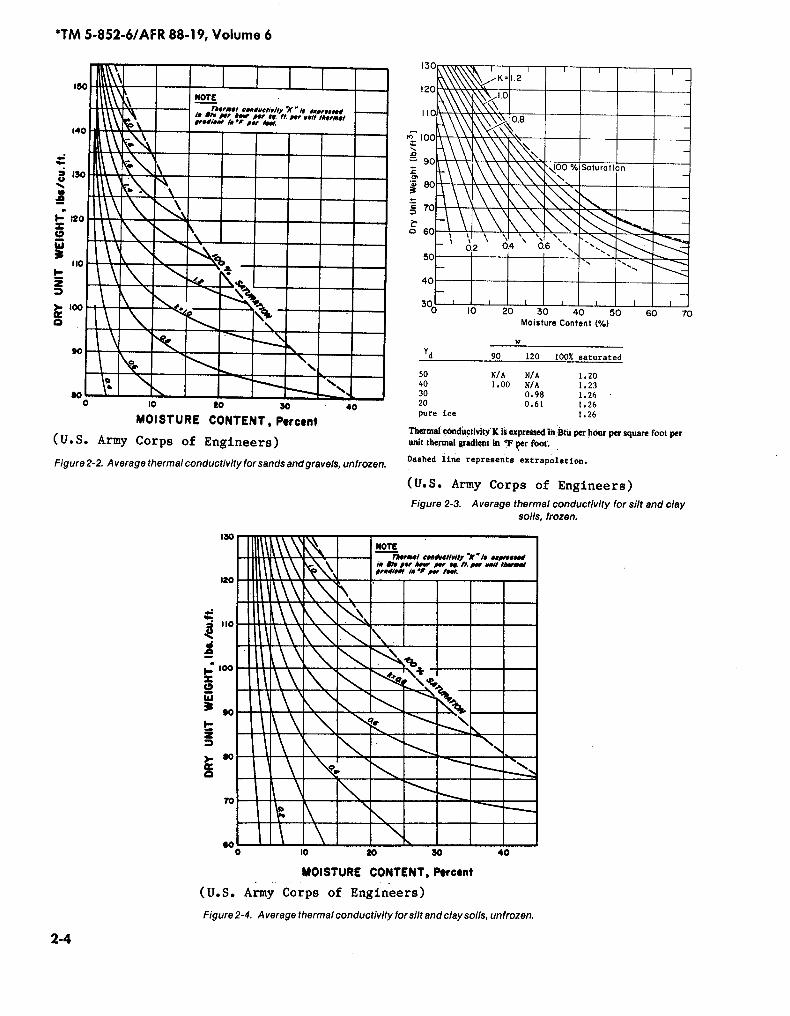
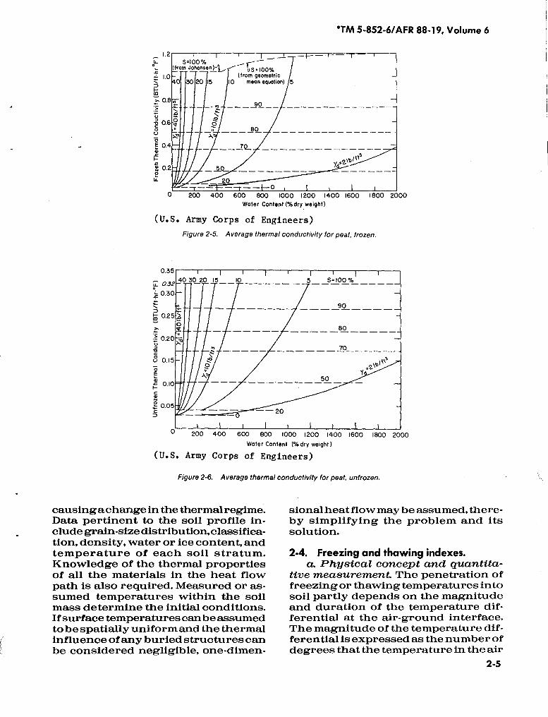
c. The thermal conductivity of soilsis dependentuponanumber offactors:density ; moisture content; particleshape; temperature ; solid, liquid andvapor constituents; and the state ofthepore water, whether frozen or unfrozen.Average values, expressed in Btu/fthour °F, for frozen andunfrozen granu-lar soils, silts and clays should be readfrom figures 2-1 through 2-4. Thecharts for sandsand gravelsare applic-able when the silt and clay contenttogether make up less than20% of thesoil solids. The charts for silt and clayare applicable when that fraction is at

' least 50%. For intermediate silt-clayfractions, it is recommended that thesimple average of the values for thetwo sets of charts be used. In all cases,the error in the thermal conductivityestimates may be ±25%, and evenhigher whenthe percentage of quartzgrains in the soil is exceptionally highor low. Figures 2-5 and 2-6 presentesti-mates of the average thermal conduc-tivity of frozen and unfrozen peat. Anexcellent source of data for dry con-struction materials is the ASHRAHGuide and Data Book. Thermal con-ductivity values for a number of com-mon construction materials are listedin table 2-2.

d. The latent heat of fusion is theamount of heat required to cause aphase change in soil moisture. Thisamount of heat does not change thetemperature of the system whenfreezing or thawing takes place. Thegravimetric latent heat of fusion ofwater is assumed to be 144 Btu/lb . Theamountofheat energy required to con-vert 1 ft of water to -ice is (144 X 62.4 =)9000 Btu/ft3 and to change 1 ft3 of ice towater is (144 X 0.917 X 62.4 =) 8240Btu/ft3. (Note: The density ofwater 62.4lb/ft3 and that of pure ice Is 57.2 lb.ft3) .

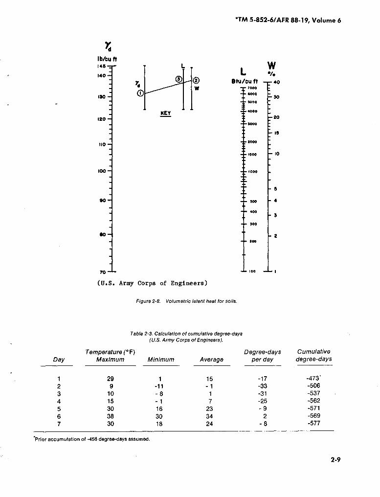
e. Figures 2-7 and 2-8 may be usedto determine the average volumetricheat capacity and volumetric latentheat of fusion, respectively, of moistsoils.

f. Thefollowingexampleillustratesthe significance of latentheatoffusionrelative to the volumetric heat capacityfor a moist soil . Assume a soil having a

dry unitweightof1201b/ft3 andawatercontent of 15 percent. Its volumetriclatent heat of fusion, L, is (144 X 120 X0.15 =1 2592 Btu/ft3 and its average volu-metric heat capacity, C, is (120[0.17 +0.75 X 0.15] =) 33.9 Btu/ft3 OF. The quan-tity of heat required to change thephase of pore water in 1 ft3of this soil at32°F is the same as that required tocause a temperature change of(2592/33.9 =) 76 .4'F when a phasechange is not involved.2-3 .

Fundamental considerations.a. Theoretical basis. The freezing

or thawing of soils is the result of re-moving or adding heat to an existingsoil mass . The movement of heat isalways inthe direction oflower temper-ature. The time rate of change of heatcontent depends on the temperaturedifferential in the direction of heatflowand on the thermal properties of thesoil .

b. Physical factors and data re-quired. Calculation of the depth offreeze or thaw is based on knowledgeof the physical and thermal propertiesof the soil in the profile, the existingthermal regime, and the nature andduration of boundary conditions

150

0 I I14

13

09T

08 e

6

50

*TM 5-852-6/AFR 88-19, Volume 6

0 10 20 30 40 50Moisture Content (%)

Thermal conductivity K is expressed in Btu per hour per square foot perunit thermal gradient in °F per foot .Dashed line represents extrapolation .

(U .S . Army Corps of Engineers)

Figure 2-1. Average thermal conductivity for sands andgravels, frozen.

60 70

0

0

2-3

\\~I2.0

1 .8

1100%/Saturation

0.2 o . s o.s \

*TM 5-852-6/AFR 88-19, Volume 6

uW

3H2

14

130

3- 100

0

2-4

90

so0 10 20 30

MOISTURE CONTENT, Percent(U .S . Army Corps of Engineers)

Figure 2-2. Average thermal conductivity for sands andgravels, unfrozen .

w

IC73z

0

40

10

t0

130

12

0W 10va 90La3 80

70

0 60

50

40

300

30

MOISTURE CONTENT, Percent

(U.S. Army Corps of Engineers)

Figure 2-4. Average thermalconductivity forsiltand clay soils, unfrozen .

10 20 30 40 50 60 70Moisture Content (°/,)

w

ThermalconductivitYK is expressed'iq :$tu perhour per square foot perunit thermal gradient in °F per foot.Dashed line represents extrapolation.

(U.S . Army Corps of Engineers)Figure 2-3.

Average thermal conductivity for silt and claysoils, frozen.

40

;0BEEN,E~ rrrr'

i

~.eGil~y K"li .yrnHl

0

n /1I usit POWINNOM

WIV

LIM

i

' 1-

iav

roenwr it"r. ..,nmn

i

NE

20111I"� .r ~ H. hr .MI lMrwal4 rs .~

110 �I"�

00 1111,101k0m --

90

so 111W 0

7001,,_ ' ~~-

aa ""

d 90 120 100% saturated

50 N/A N/A 1 .2040 1.00 N/A 1 .2330 0.98 1 .2620 0 .61 1 .26pure ice 1 .26

(U .S . Army Corps of Engineers)

causingachange in the thermal regime .Data pertinent to the soil profile in-clude grain-size distribution, classifica-tion, density, water or ice content, andtemperature of each soil stratum .Knowledge of the thermal propertiesof all the materials in the heat flowpath is also required. Measured or as-sumed temperatures within the soilmass determine the initial conditions .Ifsurface temperatures can beassumedto be spatially uniform and the thermalinfluence ofany buried structurescanbe considered negligible, one-dimen-

(U.S. Army Corps of Engineers)

_0200 400 600 800 1000 1200 1400 1600

Water Content (%dry weight)

Figure 2-5.

Average thermal conductivity for peat, frozen .

600 800 1000 1200 1400Water Content (%dry weight)

Figure 2-6.

Average thermal conductivity for peat, unfrozen.

'TM 5-852-6/AFR 88-19, Volume 6

1800 2000

sional heat flowmaybeassumed, there-by simplifying the problem and itssolution.

2-4.

Freezing and thawing indexes.a. Physical concept and quantita-

tive measurement. The penetration offreezing or thawing temperatures intosoil partly depends on the magnitudeand duration of the temperature dif-ferential at the air-ground interface.The magnitude of the temperature dif-ferential is expressed as the number ofdegrees that the temperature in the. air

2-5

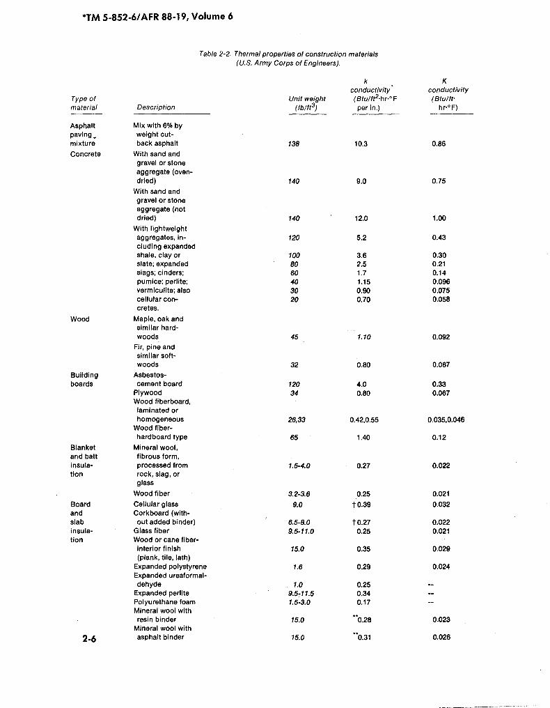
*TM 5-852-6/AFR 88-19, Volume 6

Table 2-2. Thermal properties of construction(U.S . Army Corps of Engineers) .

materials

k Kconductivity conductivity

Type of Unit weight (Btulft2 -hr"° F (Btulft "material Description (Iblit3) per in .) hr-OF)

Asphalt Mix with 6% bypaving . weight cut-mixture back asphalt 138 10.3 0 .86Concrete With sand and

gravel or stoneaggregate (oven-dried) 140 9 .0 0.75

With sand andgravel or stoneaggregate (notdried) 140 12.0 1 .00

With lightweightaggregates, in- 120 5 .2 0.43cluding expandedshale, clay or 100 3.6 0.30slate ; expanded 80 2 .5 0 .21stags ; cinders ; 60 1 .7 0 .14pumice; perlite ; 40 1 .15 0.096vermiculite ; also 30 0.90 0.075cellular con- 20 0.70 0.058cretes .

Wood Maple, oak andsimilar hard-woods 45 1.10 0.092

Fir, pine andsimilar soft-woods 32 0.80 0.067

Building Asbestos-boards cement board 120 4.0 0 .33

Plywood 34 0.80 0.067Wood fiberboard,laminated orhomogeneous 26,33 0.42,0 .55 0.035,0.046Wood fiber-hardboard type 65 1 .40 0 .12

Blanket Mineral wool,and batt fibrous form,insula- processed from 1 .5-4.0 0.27 0.022tion rock, slag, or

glassWood fiber 3.2-3.6 0.25 0.021

Board Cellular glass 9.0 1' 0.39 0.032and Corkboard (with-slab out added binder) 6.5-8.0 10.27 0.022insula- Glass fiber 9.5-11 .0 0.25 0.021tion Wood or cane fiber-

interior finish 15.0 0.35 0.029(plank, tile, lath)Expanded polystyrene 1 .6 0.29 0.024Expanded ureaformal-dehyde 1 .0 0.25 --Expanded perlite 9 .5 "11 .5 0.34 --Polyurethane foam 1.5-3.0 0.17 --Mineral wool withresin binder 15.0 0.28 0.023

Mineral wool with2-6 asphalt binder 15.0 0.31 0.026

Valuesfork are fordrybuilding materials at a meantemperatureof75°F exceptas noted; wet conditions will adversely affect values ofmany of these materials.

t Mean temperature of 60° F.

Mean temperature of 320 F.

or at the ground surface is above (posi-tive) or below (negative) 32°F, the as-sumed freezing point of water. Theduration is expressed in days.

b. Air freezing index (F) and airthawingindex(1). The air freezing andair thawing indexes, as defined in TM5-862-1/AFR 88-19, Volume 1, may bedetermined by the following methods.

(1) Summation of degree-days offreeze and thaw from average dailytemperatures. If T1 is the maximumdaily air temperature and T2 is theminimum daily air temperature. theaverage daily air temperature T, maybe taken as 1/2 (TI + T2), and thenumberof degree-days for the day is (T -_32) .The summation of the degree-days for"a freezing or thawingseason gives theair freezing or air thawing. Index.Table 2-3 illustrates the method usedto obtain the summation ofdegree-daysfor a1-week period, assuming that-456degree-days had been accumulatedsince freezing began.Anaverage dailytemperature basedonhourly tempera-tures would be slightly moreaccurate,but such precision is not usually war-ranted. The negative sign, indicating

freezing degree-days, is usuallyomitted.

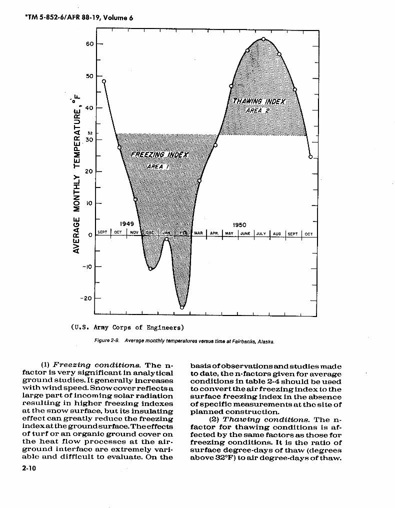
(2)Calculation fromaverage month-ly temperatures . The freezing orthawing index may be calculated bydetermining the area between the 32°Fline and the curve of average monthlytemperature and time, taken over theappropriate season . The area may bedetermined by planimeter or a simpleapproximation rule (Simpson's rule,midordinate rule, etc.) . The areas areexpressed in units of degree-days, re-sulting in asummation of degree-daysor a freezing or thawing index. For anexample refer to figure 2-9, a plot ofthe monthly average temperatures atFairbanks, Alaska, from September1949 to October 1950. Determination ofareas by planimeter gave a freezingindex of -5240 degree-days and athawing index of +3420 degree-days.Theuse ofSimpson's rule gave a freez-ing index of -5390andathawingindexof +3460 degree-days. Either pair ofindices is adequate for computations.

c. Surfacefreezing and surface-thawingindexes. For determining theheat flow within the soil, it is neces-

'TM 5-852-6/AFR 88-19, Volume 6 '

2-7

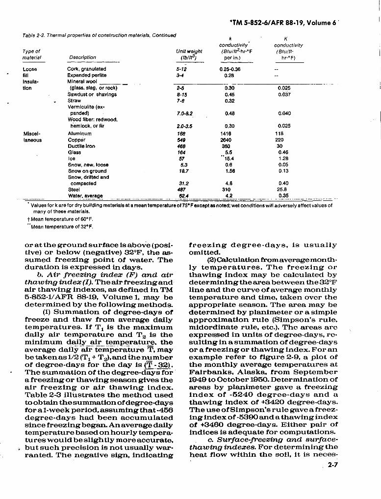
Table 2-2.

Type ofmaterial

Thermal properties of construction materials,

Description

Continued

Unit(Iblft3)

weight

kconductivity'(Btulft2-hr "°Fper in.)

Kconductivity(Btulft-

hr-°F)

Loose Cork, granulated 5-12 0.25-0.36 --fill Expanded perlite 3-4 0.28 --Insula- Mineral wooltion (glass, slag, or rock) 2-5 0.30 0.025

Sawdust or shavings 8-15 0.45 0.037Straw 7-8 0.32Vermiculite (ex-panded) 7.0-8.2 0.48 0.040Wood fiber: redwood,hemlock, or fir 2.0-3.5 0.30 0.025

Miscel- Aluminum 168 1416 118laneous Copper 549 2640 220

Ductile Iron 468 360 30Glass 164 5.5 0.46Ice 57 ~15.4 1 .28Snow, new, loose 5.3 0.6 0.05Snow on ground 18.7 1.56 0.13Snow, drifted andcompacted 31.2 4.8 0.40

Steel 487 310 25 .8Water, average 62.4 4.2 0.35

*TM 5-852-6/AFR 88-19, Volume 6

2-8

130

120-"

100-

90--

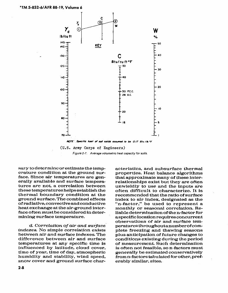
sary to determine or estimate the temp-erature condition at the ground sur-face. Since air temperatures are gen-erally available and surface tempera-tures are not, a correlation betweenthese temperatureshelps establish thethermal boundary condition at theground surface. The combined effectsof radiative, convective and conductiveheatexchangeat the air-groundinter-face often mustbe considered in deter-mining surface temperature .

d. Correlation of air and surfaceindexes. No simple correlation existsbetween air and surface indexes. Thedifference between air and surfacetemperatures at any specific time isinfluenced by latitude, cloud cover,time of year, time of day, atmospherichumidity and stability, wind speed,snow cover and ground surface char-

Btu/cu ft °FSO

40

30 RC .C .28 A.C .

20

16

7'o -L-

-

Avre.' Specific hoot of save solids assumed to be O./T ON //&. *F

(U.S . Army Corps of Engineers)

Figure 2-7.

Average volumetric heat capacity for soils.

W

90

-40

30

-20

!- 10

-5

acteristics, and subsurface thermalproperties. Heat balance algorithmsthat approximate many of these inter-relationships exist but they are oftenunwieldly to use and the inputs areoften difficult to characterize . It isrecommended that the ratio ofsurfaceindex to air index, designated as the"n-factor," be used to represent amonthly or seasonal correlation . Re-liable determination ofthe n-factor fora specific location requires concurrentobservations of air and surface tem-peratures throughoutanumberofcom-plete freezing and thawing seasonsplus anticipation of future changes toconditions existing during the periodof measurement. Such determinationis often not feasible, so n-factors mustgenerally be estimated conservativelyfrom n-factors tabulated for other, pref-erably similar, sites .

rIb/cu ft

140 -I

130-

120-

too-

too-

90-

Go-

-PO -"A.-

Prior accumulation of -456 degree-days assumed.

KEY

L W0

Btu/cu ft -t- 40

"TM 5-852-6/AFR 88-19, Volume 6

(U .S . Army Corps of Engineers)

Figure 2-8.

Volumetric latent heat for soils.

Table 2-3. Calculation of cumulative degree-days(U.S. Army Corps of Engineers).

2-9

DayTemperature (° F)

Maximum Minimum AverageDegree-days

perdayCumulativedegree-days

1 29 1 15 -17 -473 *2 9 -11 - 1 -33 -5063 10 - 8 1 -31 -5374 15 - 1 7 -25 -5625 30 16 23 - 9 -5716 38 30 34 2 -5697 30 18 24 -8 -577

*TM 5-852-6/AFR 88-19, Volume 6

2-10

wWSI-QW0-MWE-

JSI-ZO

WQSWQ

60

50

40

32

30

20

10

0

-20

(U.S . Army Corps of Engineers)Figure 2-9.

Average monthly temperatures versus time at Fairbanks, Alaska.

(1) Freezing conditions. The n-factor is very significant in analyticalground studies. It generally increaseswith wind speed. Snowcover reflectsalarge part of incoming solar radiationresulting in higher freezing indexesat the snow surface, but its insulatingeffect can greatly reduce the freezingindexat theground surface. The effectsof turf or an organic ground cover onthe heat flow processes at the air-ground interface are extremely vari-able and difficult to evaluate. On the

basis ofobservations and studies madeto date, the n-factors given for averageconditions in table 2-4 should be usedto convert the air freezing index to thesurface freezing index in the absenceof specific measurements at the site ofplanned construction.

(2) Thawing conditions. The n-factor for thawing conditions is af-fected by the same factors as those forfreezing conditions . It is the ratio ofsurface degree-days of thaw (degreesabove 32°F) to air degree-days ofthaw.

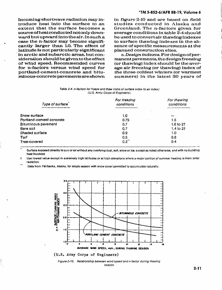
Incoming shortwave radiation may in-troduce heat into the surface to anextent that the surface becomes asource ofheatconductednotonly down-ward butupward into the air. In such acase the n-factor may become signifi-cantly larger than 1.0. The effect oflatitude is not particularly significantin arctic and subarctic areas, but con-sideration shouldbegiven to the effectof wind speed. Recommended curvesfor n-factors versus wind speed forportland-cement-concrete and bitu-minous-concrete pavements areshown

t

"TM 5-852-6/AFR 88-19, Volume 6

in figure 2-10 and are based on fieldstudies conducted in Alaska andGreenland. The n-factors given foraverage conditions in table 2-4 shouldbe used to convertair thawingindexesto surface thawing indexes in the ab-sence of specific measurements at theplanned construction sites.

e. Designindexes. Fordesign ofper-manentpavements, the design freezing(or thawing) index should be the average air freezing (or thawing) index ofthe three coldest winters (or warmestsummers) in the latest 30 years of

Surface exposed directly to sun or air without any overlying dust, soil, snow or ice, except as noted otherwise, and with no buildingheat involved .

Use lowest value except in extremely high latitudes or at high elevations where a major portion of summer heating is from solarradiation.

Data from Fairbanks, Alaska, for single season with snow cover permitted to accumulate naturally .

X

a~rcN

C

0 2 4 6 6 10 12 14AVERAGE WIND SPEED, mph, DURING THAWING SEASON

(U.S. Army Corps of Engineers)Figure 2-10.

Relationship between wind speed and n- factor during thawingseason .

16

2-1 1

3.0I

2.6

2.0 ~~,S

ICANCRETE

1.0

`PoWTCAA9 CEMENT CONCRETE

Table 2-4.

Type of surface

n-factors for freeze and thaw (ratio ofsurface index to air index)(U.S. Army Corps of Engineers).

For freezingconditions

For thawingconditions

Snow surface 1 .0 _-Portland-cement concrete 0.75 1 .5Bituminous pavement 0.7 1 .6 to 2tBare soil 0.7 1 .4 to 2tShaded surface 0.9 1 .0Turf 0.5 0.8Tree-covered 0.3 ** 0.4

'TM 5-852-6/AFR 88-19, Volume 6

record . If 30 years of record are notavailable, the air freezing (or thawing)index for the coldest winter (orwarmest summer) in the latest 10-yearperiod may be used. For design offoundations for average permanentstructures, the design freezing (orthawing) index should be computedfor the coldest (or warmest) winter in30 years of record or should be esti-mated to correspond with this fre-quency ifthe number of years of recordis limited . Periods of record usedshould be the latest available. To avoidthe necessity for adopting a new andonly slightly different freezing (orthawing) index each year, the designindex at a site with continuing con-

Wh

9000

xWOZ

Z

XQ

I Cg000

. e0001-

7000F-

5000

400,03000

(AmAloo

o(BEMEL)

4

(NORrNWAY) o

/ o(KOrZESUE)(FAIRBANKS!

(rHIXE) o

I(BARROW!o

/6(Fr YUKON/

(BETTLES)

NOTE .' rhulr, bnenlond dolo from /952 through 1961 .

I

I

I

I

I8000 9000000 5000

MEAN AIR-FREEZING INDEX, Degree-days(U.S . Army Corps of Engineers)

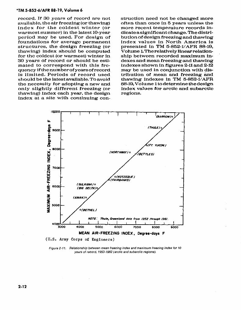
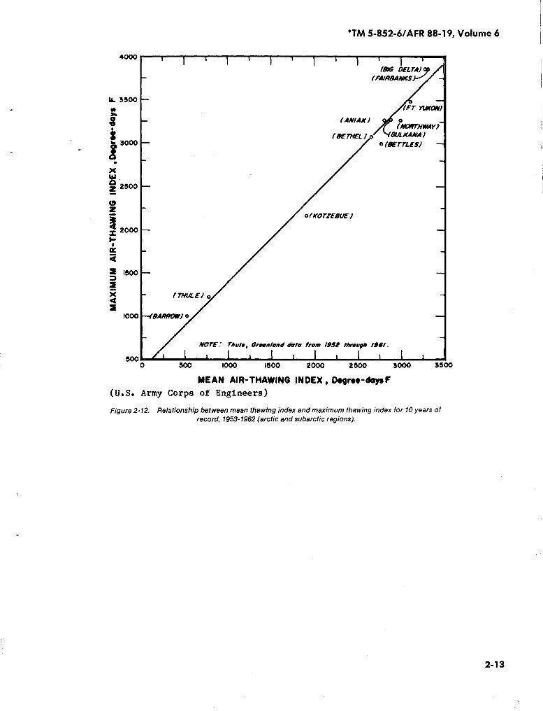
struction need not be changed moreoften than once in 5 years unless themore recent temperature records in-dicate a significant change. The distri-bution ofdesign freezingandthawingindex values in North America ispresented in TM 5-862-1/AFR 88-19,Volume 1. Therelatively linear relation-ship between recorded maximum in-dexes and mean freezing and thawingindexes shown in figures 2-11 and 2-12may be used in conjunction with dis-tribution of mean and freezing andthawing indexes in TM 5-862-1/AFR88-19,Volume 1 to determine the designindex values for arctic and subarcticregions.

6000 7000

F

Figure 2-11 .

Relationship between mean freezing index andmaximum freezing index for 10years of record, 1953-1962 (arctic and subarctic regions) .

NWW

W(6ULKANA) o

6000 (B/6 DELTA! o,Q

IL 3500

r

X

z 2500

Z

XQ

4000

3000

1500

1000

500

( THUL E) 0

-IBARROWI0/

0(KOTIEBUE)

(BW OELWT(FAIRBAAWS)

(FT. YUIfQY)

(ANIAK) 0Ir (MOPrHWAY1

(BETNEL) a' VG7/LKANA)0wrnESI

NOTE .' Mule, areonlend dolo from 1952 /Amuph /of/ .

Imo_- L. j

I

1

I

1

I

I

I

t0 500 1000 1500 2000 2500 3000 3500

MEAN AIR-THAWING INDEX, D"rwdoysF(U.S. Army Corps of Engineers)

*TM 5-852-6/AFR 88-19, Volume 6

Figure 2-12.

Relationship between mean thawing index and maximum thawing index for 10 years ofrecord, 1953-1962 (arctic and subarctic regions) .

CHAPTER 3

ONE-DIMENSIONAL LINEAR AND PERIODIC HEAT FLOW

3-1 .

Thermal regime.The seasonal depths of frost and thawpenetration in soils depends upon thethermal properties of the soil mass, thesurface temperature (upper boundarycondition) and the thermal regime ofthe soil at the start of the freezing orthawing season . Many methods areavailable to estimate frost and thawpenetration depths and surface tem-peratures . Some of these are sum-marized in appendix B. This chapterconcentrates on some techniques thatrequire only relatively simple handcalculations . For the computationalmethods discussed below, the initialground temperature isassumed to uni-formly equal the mean annual air tem-perature of the particular site underconsideration . The upper boundarycondition is represented by the sur-face freezing (or thawing) index.

3-2 .

Modified Berggren equation.a. The depth to which 32°F tem-

peratures will penetrate into the soilmass is based upon the "modified"Berggren equation, expressed as:

48KnF

Lor

(eq3-1)

48 K nl

Lwhere

X= depth of freeze or thaw (ft)K= thermal conductivity of soil

(Btu/ft hr °F)L = volumetric latent heat of fusion

(Btu/ft3)n=conversion factor from air

index to surface index (dimen-sionless)

F= air freezing index (°F-days)I = air thawing index (°F-days)

'TM 5-852-6/AFR 88-19, Volume 6

= coefficient that considers theeffect of temperature changesin the soil mass (dimensionless).

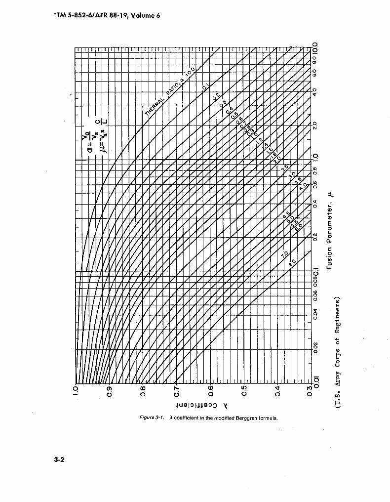
The A coefficient is a function of thefreezing (or thawing) index, the meanannual temperature of the site, and thethermal properties of the soil. Freezeand thaw of low-moisture-content soilsin the lower latitudes is greatly in-fluenced by this coefficient . Itisdeter-minedby two factors: the thermal ratioa and the fusion parameter /j. Thesehave been defined in paragraph 2-1.Figure 3-1 shows A as a function of aand N.

b . A complete development of thisequation and a discussion of the neces-sary assumptions and simplificationsmade during its development are notpresented here. A few of the more im-portant assumptions and some of theequation limitations are discussedbelow. The assumptions and limita-tions apply regardless ofwhether theequation is used to determine the depthof freeze or the depth ofthaw.

(1)Assumptions. The mathematicalmodel assumes one-dimensional heatflow with the entire soil mass at itsmeanannual temperature(MAT) priorto the start of the freezing season. Itassumes thatwhenthe freezing seasonstarts, the surface temperaturechanges suddenly (as a step function)from the mean annual temperature toa temperature v3 degrees below freez-ing and that it remains at this newtemperature throughout the entirefreezing season. Latent heat affects themodel by acting as a heat sink at themoving frost line, and the model as-sumes that the soil freezesata tempera-ture of 32°F .

(2) Limitations. The modifiedBerggren equation is able to determinefrost penetration in areas where theground below a depth of several feet

*TM 5-852-6/AFR 88-19, Volume 6

3-2

IIIMIdMI M%I/ImpAPEFAMUFAFI19,aPAPIMAPOAF

1111~II~D~

N MINE

115111111211p

111111111111111!1

10110. Ap

1 0;,

"/~~~~~

lI/I%/I%I MEN.MMwMII0;WAMIIW,I"I%IL//w%/

MAI

OPFA POPPAP'A NFAOAF-FINEFOR JIPPAFA

'A

IF-

I's 004 AP04

n~~r~i~r/ya~inztiRai~azra~i~w~an

~~I

AlaiNII~~

WONFA

'All,IPI

4ua!o1j;aOO

Figure 3-1 .

A coefficient in the modified Berggren formula.

N

W4-10

a0U

remains permanently thawed, or todetermine thaw penetration in areaswhere the ground below a depth .ofseveral feet remains permanentlyfrozen. These two conditions are simi-lar in that the temperature gradientsare of the same shape, although re-versed with respect to the 32°F line . Nosimpleanalyticalmethod exists to deter-mine the depth of thaw in seasonalfrost areas or the depth of freeze inpermafrost areas, and such problems ,should be referred to HQDA (DAEN-ECE-G) or HQAFESC. Numerical tech-niques and computer programs areavailable to solve more complex prob-lems. AppendixB discusses some ther-mal computer models for computingfreeze and thaw depths. The modifiedBerggren equation cannotbe used suc-cessfully to calculate penetration overparts of the season. The modifiedBerggren equation does not accountfor any moisture movement that mayoccur within the soil. This limitationwould tend to result in overestimatedfrost penetration (if frost heave is sig-nificant) or underestimated thawpenetration.

(3) Applicability. The modifiedBerggren equation is most often applic-able in either of two ways: to calculatethe multi-year depth of thaw in perma-frost areas or to calculate the depth ofseasonal frost penetration in seasonalfrost areas. It is also sometimes used tocalculate seasonal thaw penetration(active layer thickness) in permafrostareas.

3-3.

Homogeneous soils.The depth of freeze or thaw in onelayer ofhomogeneoussoilmaybe deter-mined by means of the modifiedBerggrenequation.A thin bituminousconcrete pavement will not affect thehomogeneity of this layer in calcula-tions, but a portland-cement-concretepavement greater than 6 inches thickshould be treated as a multilayeredsystem. In this example for homoge-neous soils, determine the depth of

. frost penetration into a homogeneoussandy silt for the followingconditions:

-Mean annual temperature(MAT) = 37.2°F .

*TM 5-852-6/AFR 88-19, Volume 6

-Surface freezing index (nF) _2600 degree-days.

-Length of freezing season (t)= 160 days.

-Soil properties: yd =1001b/ft3, w= 16%.

The soil thermal properties are asfollows:

-Volumetric latent heat of fusion,L = 144(100)(0.16) = 2160 Btu/ft3.

(eq. 3-2).-Average volumetric heatcapacity,Cavg =100[0.17++(0.75X0.l5)]= 28.3 Btu/ft3 -F .

(eq3-3)-Average thermal conductivity,Kf = 0.80 Btu/ft hr °F (fig. 2-3)Ku = 0.72 Btu/ft hr °F (fig . 2-4)Kav = 1/2 (Ku +Kf) --' 0.76 Btu/fthr °f'.

The ,l coefficient is as follows:-Average surface temperaturedifferential,

vs = nF/t - 2600/160- 16.6°F (16.6°F below 32°F).

(eq3-4)-Initial temperature differential,vo - MAT -32 - 37.2-32.0 =6.2°F (6 .2° above 32°F).

(eq3-6)-Thermal ratio,a = vo/vs = 6.2/16.6 - 0.33.

(eq3-6)-Fusion parameter,p - vs (C/L) - 16.6(28.2/2160) - 0.20.

(eq3-7)-Lambda coefficient,.1 - 0.89 (fig. 3-1) .

(eq3-8)Estimated depth of frost penetration,

X

48KnF= 0.89J 48(0.76)(2600)

=~

5.8 ftL

2160

(eq3-8

3-4.

Multilayer soils.A multilayer solution to the modifiedBerggren equation is used for non-homogeneous soils by determiningthat portion of the surface freezing (orthawing) index required to penetrateeach layer. The sumof the thicknessesof all the frozen (or thawed) layers isthe depth of freeze (or thaw). Thepartial freezing (or thawing) index re-quired to penetrate the top layer isgiven by

Lid, RyF1 (or 11) -

2

(

2

)

(eq3-10)24a 1

3-3

'TM 5-852-6/AFR 88-19, Volume 6

wheredl = thickness of first layer (ft)R1 = dl/K1 = thermal resistance of

first layer.The partial freezing (or thawing) indexrequired to penetrate the second layeris

The partial indexrequired to penetratethe nth layer is:

whereIR is the total thermal resistanceabove the nth layer and equals

3-4

L2d2 R2F2 (or I2 ) = .

(111+

-) .24x2 2

RnFn (or In) -

(MR +

- )24.12 2

Lndn

(eq 3-11)

(eq 3-12)

R1 + R2 + R3 . . . + Rn.1 "

(eq 3-13)

The summation of the partial indexes,F 1 +F2 + F3 . ..+Fn(orI 1 +I2+13 .. .+ In)

Is equal to the surface freezing indexthawing index) .

a. In this example, determine thedepth of thaw penetration beneath abituminous concrete pavement for thefollowing conditions:

-Meanannual temperature (MAT)= 12°F.

-Air thawing index (I)= 780 degree-days.

-Average wind speed in summer7.5 miles per hour (mph).

-Length of thaw season (t)= 105 days.

-Soil boring log-.

(eq 3-14)

~In accordance with Unified Soil Classification System .

Since awindspeed of 7-1/2 mph resultsin an n-factor of 2.0 (fig. 2-10), a surfacethawing index nI of 1560 degree-daysis used in the computations. The vs, voand a values are determined in the sameway as those for the homogeneous case:

vs- 1560/105 = 14.8°F

(eq 3-15)vo= 12.0 - 32.0 = 20.0°F

(eq 3-16)a s 20.0/14 .8 - 1.35 .

(eq3-17)The thermal properties C, K and L ofthe respective layers are obtained fromfigures 2-1 through 2-8.

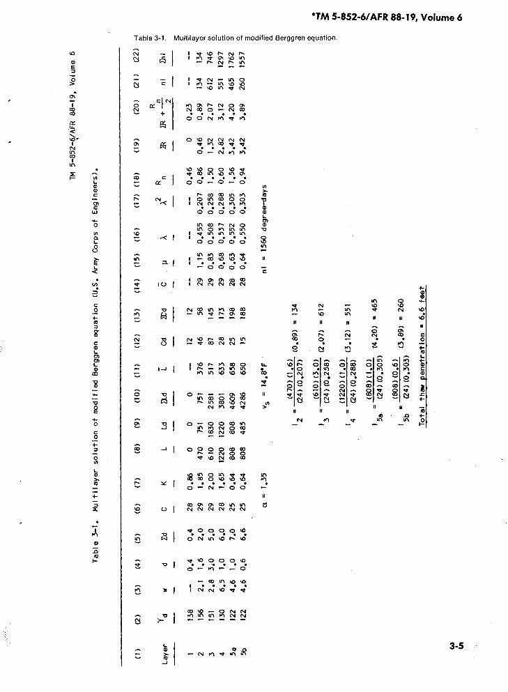
b. Table 3-1 facilitates solution ofthe multilayer problem, and in the fol-lowing discussion, layer 3 is used toIllustrate quantitative values. Columns9, 10, 12 and 13 are self-explanatory.Column 11, T:, represents the averagevalue of L for a layer and is equal toELd/ld (2581/5.0 = 517) . Column 14, Zs,represents the average value of C andis obtained from XCd/ld (145/5.0 = 29).Thus T: and -C represent weightedvalues to a depth of thaw penetrationgiven by Ed, which is the sum of alllayer thicknesses to that depth.The fusion parameter p for each layeris determined from

v8 (C /L) = 14.8 (29/517) = 0.83 .

(eq 3-18)The A coefficient is equal to 0.508 fromfigure 3-1 . Column 18, Rn, is the ratiod/K and for layer 3 equals (3.0/2.0) or1.5. Column 19, FR, represents the sumof the Rn valuesabove the layer underconsideration . Column 20, IR + (Rn/2),equals the sum of the R n values abovethe layer plus one-half the Rn value ofthe layer being considered. Fog ,ayer 3this is [1.32 + (1.50/2)] = 2.07. Column 21,nI, represents the number of degree-days required to thaw the layer beingconsidered and is determined from

LayerDepth

(ft) Material'Dry unit weight

(Iblft3)Water content

(%)

1 0.0-0.4 Asphaltic concrete 138 _-2 0.4-2.0 GW-G P 156 2.13 . 2.0-5.0 GW-G P 151 2.84 5.0-6.0 SM 130 6.55 6.0-8.0 SM-SC 122 4.66 8.0-9.0 SM 116 5.2

TM5-

852-

6/AF

R88

-19,

Volume

6

w c m 0 " 3 0 a o

70

Tota

lth

awpenetration

=6,

6fe

etO C

Tabl

e3-

1,Mu

ltil

ayer

solu

tion

ofmodified

Berg

gren

equa

tion

(U.S

.Army

Corps

ofEngineers)

.

(1)

(2)

(3)

(4)

(5)

(6)

(7)

(8)

(9)

(10)

(11)

(12)

(13)

(14)

(15)

(16)

(17)

(18)

(19)

(20)

(21)

(22)

RLa

yer

Yd

wd

EdC

KL

LdELd

LCd

Md

CIt

.~~2

RnBR

D2+2

nlPn

I

1138

--0,

40,

428

0,86

00

0--

1212

----

----

0,46

00,23

----

2156

2,1

1,6

2,0

291,85

470

751

751

376

4658

291,15

0,45

50,207

0,86

0,46

0,89

134

134

3151

2,8

3,0

5,0

292,

0061

01830

2581

517

87145

290,83

0,508

0,25

81,50

1,32

2,07

612

746

4130

6,5

1,0

6,0

281.65

1220

1220

3801

633

28173

290,68

0,53

70,288

0,60

2,82

3,12

551

1297

5a122

4,6

1,0

7,0

250,

6480

880

846

0965

825

198

280,

630,

552

0,30

51,56

3.42

4,20

465

1762

5b122

4,6

0,6

6,6

250,

6480

848

54286

650

15188

280,

640,

550

0,30

30,94

3,42

3"89

260

1557

a=

1,35

vs=

14,8

°Fni

=1560

degr

ee-d

ays

(470)(1,6)

1__

2(2

4)(0,207)

(0"89)

=134

(610)(3,0)

I=

(2,07)

=61

23

(24)

(0.2

58)

(1220)(1,0

14_

(3'12)

=551

(24)

(0,288)

(808)(1,0)

15a

(4"20

)=

465

(24)

(0,305)

(808)(0,6)

15b

_(3

"89)

=26

24)

(0,303)

*TM 5-852-6/AFR 88-19, Volume 6

For layer 3,(610)(3.0)

The summation of the number ofdegree-days required to thaw layers 1through 4 is 1297, leaving (1560 -1297 =)263 degree-days to thaw a portion oflayer 5. A trial-and-error method is usedto determine the thickness of thethawed part of layer 5. First, it is as-sumed that 1.0 feet of layer 5 is thawed(designated as layer 5a). Calculationsindicate 465 degree-days are neededtothaw 1.0 foot of layer 5 or (465 - 263 =)202 degree-days more than available.A new layer, 5b, is then selected by thefollowing proportion

This new thickness results in 260degree-days required to thawlayer 5bor 3 degree-days less than available.Further trial-and-error isunwarrantedand the total estimated thaw penetra-tion would be 6.6 feet. A similar tech-nique is used to estimate frost penetra-tion in a multilayer soil profile.3-5.

Effect of snow and vegetative cover.Thermal properties of snowandvegeta-tive covers are extremely variable inboth time and space. Both materialstend to act as insulators and retardheat transfer at the air-ground inter-face .Infreeze-thawcomputations,snowand vegetative surface materials aretreated as separate layers in the multi-layer solution ofthe modified Berggren

3-6

Ldn1 -

(7-R +24,2

= 612 degree-days

(eq 3-19)

n13 =

(2.07)

(eq3-20)24(0.608)2

(263/466)1 .0 = 0.57 ft (try 0.6 ft) .

(eq3-21)

equation, with snow cover thicknessestimated seasonally . The tabulationbelow presents average thermal proper-ties ofsnowapplicable for calculationin the noted regions if a better database is not available. In the absence ofsite-specific data, figures 2-5 and 2-6should beused to estimate the thermalconductivities of vegetative surfacecover.3-6.

Surface temperature variations .The temperatures at the air-groundinterface are subject to daily and sea-sonal fluctuations. Precipitation, insola-tion, air temperature and turbulencecontribute to these variations in sur-face temperature. To facilitate mathe-matical calculations, twoassumptionsarecommonlymaderegarding the tem-peratures at the upper boundary : 1) asudden step change occurs in surfacetemperature or 2) the surface tempera-ture change is sinusoidal. The sinu-soidal variation of temperature over ayear closely approximatesactual condi-tions; however, it is amenable to handcalculations only if latent heat effectsare negligible . Solutions and examplesfor both conditions are given below.

a. Suddenstep change. This involvesa sudden change in the surface tem-perature of a mass thatwas initially ata constant, uniform temperature . Thesuddenstep change wasused to estab-lish the boundary conditions for heatflow in the modified Berggren equationgiven in paragraph 3-2. If the influenceof latent heat is not involved, or is as-sumed negligible, the following equa-tion may be used:

T(X t) = Ts + (To - Ts) erf (

)

(eq3-22)2 -fat

Region

Unitweight(Iblft 3 )

K(Btulft)hr ° F)

C(Btulft3 ° F)

L(Btulft3 )

Interior Alaska 16 0.11 8 2300

Canadian Archipelago,N . Alaskan coast,and temperate regions 20 0.18 10 2880

Northern Greenland 22 0.20 11 3170

where

T(X, t) = temperature at depth x, attime (°F)

TS

= suddenly applied constantsurface temperature (°F)

To

=initial uniform tempera-ture of the mass (°F)

erf

=mathematical expression,-

termed the error function,which is frequently usedin heat flow computations(dimensionless)

x

=depth below surface (ft)

h164'

I

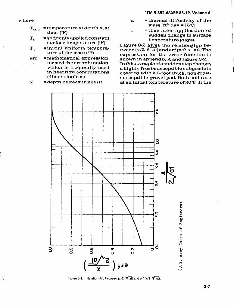
Figure 3-2.

Relationship between (x/2 Y-a-t) and erf (x/2

at).

*TM 5-852-6/AFR 88-19, Volume 6

a

= thermal diffusivity of themass (ft2/day = K/C)

t

= time after application ofsudden change in surfacetemperature (days).

Figure 3-2 gives the relationship be-tween (x/2 at) and erf (x/2 1rat) .Theexpression for the error function isshown in appendix A and figure 3-2.In thisexample ofasudden step change,a highly frost-susceptible subgrade iscovered with a 2-foot thick, non-frost-susceptible gravel pad. Both soils areat an initial temperature of 20°F . If the

0N

t0O

NO

..

v

Mb0GWWO

A.HOU

v

3-7

*TM 5-852-6/AFR 88-19, Volume 6

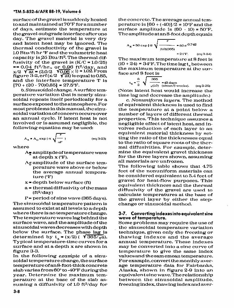
surface ofthe gravel is suddenly heatedto and maintained at 70°F foranumberof days, estimate the temperature atthe gravel-subgrade interface after oneday. The gravel material is very dryand latent heat may be ignored. Thethermal conductivity of the gravel is1.0 Btu/ft hr °F and the volumetric heatcapacity is 25 Btu/ft3. The thermal dif-fusivity of the gravel is (K/C = 1.0/25)== 0.04 ft2/hr., or 0.96 ft2/day, andx/2 at = (2.0/2 1r0.~-X 1) = 1.02 . Fromfigure 3-2, erf (x/2 -a6t) is equal to 0:85,and the interface temperature T is[70 + (20 - 70)0.851 = 27.5°F.

b. Sinusoidal change. Asurfutce tem-perature variation that is nearly sinu-soidal repeats itself periodically for asurface exposed to the atmosphere. Formost problems in this manual, the sinu-soidal variation ofconcernoccurs overan annual cycle. If latent heat is notinvolved or is assumed negligible, thefollowing equation may be used:

whereA= amplitude oftemperature wave

atdepth x (°F) .Ao amplitude of the surface tem-

perature wave above or belowthe average annual tempera-ture (°F)

x = depth below surface (ft)a = thermal diffusivity of the mass

(ft2/day)P= period of sine wave (365 days) .

The sinusoidal temperature pattern isassumed to exist at all levels to a depthwhere there is notemperaturechange.Thetemperature waves lag behind thesurface wave, and the amplitude of thesinusoidal wavesdecreases with depthbelow the surface. The phase lag isdetermined by tx = (x/2) ( 3-1r6Ua).Typical temperature-time curves for asurface and at a depth x are shown infigure 3-3.In the following example of a sinu-soidal temperature change, the surfacetemperature ofan 8-foot-thickconcreteslab varies from 60° to -40°F during theyear. Determine the maximum tem-perature at the base of the slab as-suming a diffusivity of 1.0 ft2/day for3-8

Ax = Ao exp (-x

)

(eq3-23)aP

the concrete . Theaverage annual tem-perature is [60 + (-40)1/2 = 10°F and thesurface amplitude is (60 - 10) = 50°F.The amplitude at an 8-foot depth equals

50 exp [-8 .V

= 50 e'0.742(1.0)(365)

24°F .

(eq 3-24)The maximum temperature at 8 feet is(10 + 24) = 34°F. The time lag txbetweenthe maximum temperature at the sur-face and 8 feet is

8 ~ 365tx

=43days2

n(1.0)

(about 6 weeks) .

(eq 3-25)(Note: latent heat would increase thetime lag and decrease the amplitude.)

c. Nonuniform layers. The methodof equivalent thickness is used to findthe temperature at a point below anumber of layers of different thermalproperties. This technique assumes anegligible effect of latent heat, and in-volves reduction of each layer to anequivalent material thickness by set-ting the ratio of the thicknesses equalto the ratio of square roots of the ther-mal diffusivities . For example, deter-mine the equivalent gravel thicknessfor the three layers shown, assumingall materials are unfrozen.The following table shows that 4.75feet of the nonuniform materials canbe considered equivalent to 5.4 feet ofgravel for heat-flow purposes . Thisequivalent thickness and the thermaldiffusivity of the gravel are used tocalculate temperatures at the base ofthe gravel layer by either the step-change or sinusoidal method.

3-7.

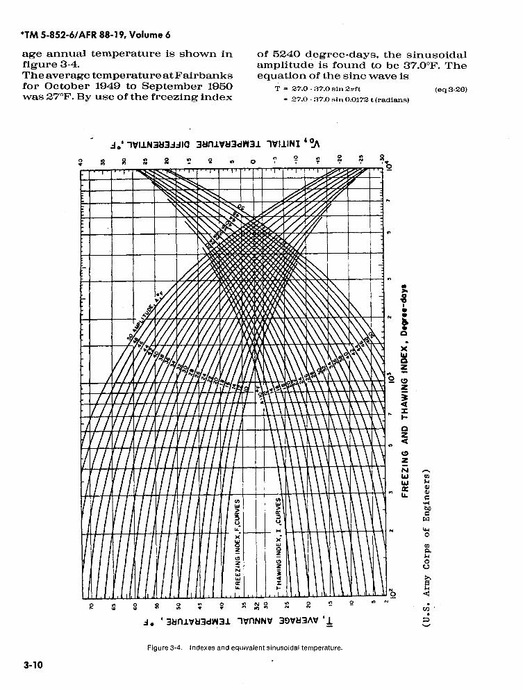
Converting indexes into equivalent sinewave of temperature.Someproblems may require the use ofthe sinusoidal temperature variationtechnique, given only the freezing orthawing indexes and the averageannual temperature. These indexesmay be converted into a sine curve oftemperature to give the same indexvalues and thesamemean temperature .For example, convert the monthly aver-age temperature data for Fairbanks,Alaska, shown in figure 2-9 into anequivalent sinewave. The relationshipbetween the sinusoidal amplitude,freezingindex, thawing indexand aver-

From figure 2-2 .tC = y d (0 .17 + w/100) .

TIME

The subscript g refers to the gravel layer and the subscript m refers to the other material layer .

"TM 5-852-6/AFR 88-19, Volume 6

FREEZING INDEX Ar DEPTH (X)

3-9

(U.S . Army Corps

Figure

of Engineers)

3-3. Sinusoidal temperature pattern .

VolumetricDry Unit Thermal heat Thermalweight, Water conductivity, capacity, diffusivity,

yd content, K C a = K/CMaterial (Ib/ft) w (%) (Btulft hr° F) (Btulft3 ° F) (ft 2/hr)Concrete -- -- 1 .0 33.0 0.033Sand 120 2 0.8* 23 t 0.035Gravel 135 4 1 .5 * 28 tx 0.054

MaterialThickness

(ft)

Thermaldiffusivity

(ft 2lhr)Equivalent gravelthickness (ft)

Concrete 1 .75 0.033 1 .3 2.3 (1 .3 X 1 .75)Sand 0.50 0.035 1 .2 0.6Gravel 2.50 0.054 1 .00 2.50

Total thickness 4.75 5.4

*TM 5-852-6/AFR 88-19, Volume 6

age annual temperature is shown infigure 3-4.Theaveragetemperature at Fairbanksfor October 1949 to September 1950was 27°F . By use of the freezing index

3- 10

O

EWA

VAF,FA

:~

~

~~~NIMIN&eINIMA iurua~

L11 ~RAM RAW\TAXU

2ManiMriiM "t~~n llWIW1 11R

MANFAM iiINTERIM""~~~~

~NaII WHEN

O

,1,' -1VI1N3a3ddl0 3an1Va3dW31 '1VIIINI 4 ?J1

N N M 2

AO O,$

o

= 27.0 - 37.0 sin 0.0172 t (radians)

10

O

N O

r

O

f?b

10

M

f

f

W~ M

N

N

d, '38f11Va3dW31 -lVnNNV 3JV83AV 'l

Figure 3-4.

Indexes and equivalent sinusoidal temperature.

of 5240 degree-days, the sinusoidalamplitude is found to be 37.0°F . Theequation of the sine wave is

T = 27.0 - 37.0 sin 2vft

(eq 3-26)

N

0

M

N

wT

4

PO

xW0Z

Z

a0Za

N

wheref = frequency, 1/365 cycles per dayt = time from origin in days. (Origin

of curve is located at a. pointwhere T intersects the averageannual temperature on its waydownward toward the yearlyminimum.)

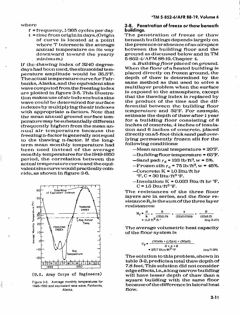
If the-thawing index of 3240 degree-days had been used,the sinusoidal tem-perature amplitude would be 35.50F.The actual temperature curve for Fair-banks, Alaska, and the equivalent sinewavecomputed from the freezing indexare plotted in figure 3-5. This illustra-tion makesuse ofair indexes buta sinewave could be determined for surfaceindexes bymultiplying the air indexeswith appropriate n-factors. Note thatthe mean annual ground surface tem-perature maybe substantially different(frequently higher) from the meanan-nual air temperature because thefreezingn-factor is generally not equalto the thawing n-factor . If the long-term mean monthly temperature hadbeen used instead of the averagemonthlytemperatures for the1949-1950period, the correlation between theactual temperature curveand the equi-valentsine curvewould practically coin-cide, as shown in figure 3-6.

60

50

.d 40

3027

r 20

0

afda0" 0

-10

-2

10

(U.S . Army Corps of Engineers)Figure 3-5.

Average monthly temperatures for1949-1950 and equivalent sine wave, Fairbanks,

Alaska .

*TM 5-852-6/AFR 88-19, Volume 6

3-8 .

Penetration of freeze or thaw beneathbuildings.The penetration of freeze or thawbeneath buildings depends largely onthe presence orabsence ofanairspacebetween the building floor and theground as discussed below and in TM5-852-4/AFM 88-19, Chapter 4.

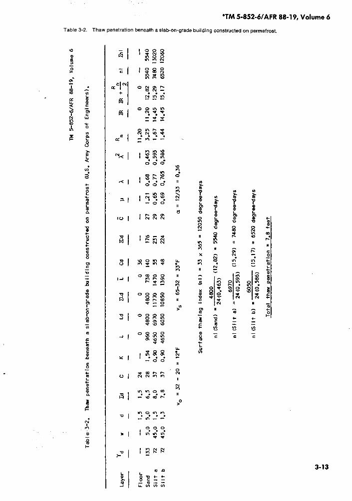
a. Building floorplaced onground.When the floor of a heated building isplaced directly on frozen ground, thedepth of thaw is determined by thesame method as that used to solve amultilayer problem when the surfaceis exposed to the atmosphere, exceptthat the thawing index is replaced bythe product of the time and the dif-ferential between the building floortemperature and 32'F. For example,estimate the depth ofthaw after 1 yearfor a building floor consisting of 8Inches of concrete, 4 inches of insula-tion and 6 inches of concrete, placeddirectly on a5-foot-thick sand pad over-lying permanently frozen silt for thefollowing conditions :

-Mean annual temperature = 20°F.-Buildingfloor temperature = 650F.-Sand pad: Yd= 133 lb/ft3, w = 5%.-Frozen silt: yd = 75 Ib/ft3, w = 45%.-Concrete: K = 1.0 Btu/fthr

'F, C = 30 Btu/ft3 oF.-Insulation: K = 0.033 Btu/ft hr'F,C = 1.5 Btu/ft3 'F.

The resistances of the three floorlayers are in series, and the floor re-sistanceB. f isthesumofthe three layerresistances:

Rf . d +

8

+

4

+

ak (12)(1 .0) (12)(0.03:3) (12)(1.0)

= 11.2 ft2 ft °

(eq 3-27)

The average volumetric heat capacityof the floor system is

(30)(8) + (1,6)(4) + (30)(F3)Cr8+4+g

= 23.7 Btu/ft3,F

(eq 3-28)

Thesolution to this problem, shown intable 3-2, predicts a total thaw depth of7.8 feet. This solution did not consideredge effects, i.e.,along narrow buildingwill have lesser depth of thaw than asquare building with the same floorbecause ofthe difference in lateral heatflow.

3-1 1

Sine Waveof Equivalent Indexes

THAWINGINDEX

--- TAvg Annual/~ Temp

FREEZINGINDEX /

Avg.Temperature

L_ ILQD©~lM 138~© o-.

1949 1950

*TM 5-852-6/AFR 88-19, Volume 6

3-12

IJL0

60

50

TT--T_ - _ i

SINE WAVE EOUIVALEN T(AMPL/TUOE 37 °F)

OCT

(U .S . Army Corps of Engineers)Figure 3-6 .

Long-term mean monthly temperatures and equivalent sine wave, Fairbanks, Alaska.

b. Airspace below building(1)Anunskirtedairspacebetween

the heated floor of building and theground will help preventdegradationofunderlying permafrost.Theairspaceinsulates the building floor from theground and acts as a convective pas-sage for flow of cold air that dissipatesheat from the floor system and theground.Thedepthofthaw is calculatedby means of the modified Berggrenequation for either ahomogeneous ormultilayered soil system, as applicable.An n-factor of 1.0 is recommended todetermine the surface thawing indexbeneath theshaded areaof an elevatedbuilding.

(2) There is no simple mathemati-cal expression for analyzing the heatflow in a ventilated floor system thathas ducts or pipes installed within theflooror at somedepthbeneaththefloor,with air circulation induced by stackeffect. The depth to which freezingtemperatures will penetrate is com-putedwith themodifiedBerggren equa-tion, except that theair freezing indexat the outlet governs. This index isinfluenced by anumber of design vari-ables, i.e., average daily air tempera-tures, inside building temperatures,floor and duct or pipe system design,temperature and velocity of air in thesystem, and stack height. Cold air

W

Q

4

MEAN TEMPERATURE

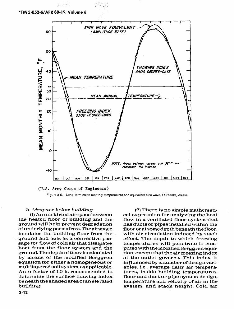
THAWING INDEX3400 DEGREE-DAYS

W3230a

MEAN ANNUAL TEMPERATUREW 26 .2

H

J 20 FREEZING INDEX5300 DEGREE-DAYS

HZO

IO

ZW

0

NOTE. Areas between curves and 32°F linerepresent the indexes.

-10 i*

SEPT I OCT I NOV -I DEC JAN I FEB I MAR I APR I MAY JUNE__ 1 JULY1AUG A SEPT

w w

TM5-

852-

6/AF

R88

-19,

Volume

6

Tabl

e3-

2.

Thaw

pene

trat

ion

beneath

aslab-on-grade

building

constructed

onpe

rmaf

rost

(U.S

.Army

Corps

ofEn

gine

ers)

,

m w N m a 3 "" w J m m w a 0 d n.

Surface

thawing

inde

x(n

l)=

33x36

5=

1205

0degree-days

a48

00ni

(San

d)-

24(0

,463

)(1

2.8

2)=

5540

degree-days

6970

nI(S

ilt

a)=

24(0

.593

)(1

5.29)

=74

80degree-days

m a 060

50ni(S

ilt

b)-

(15,17)

-6520

degree-days

mN

24(0

.586

)3

am

Total

thaw

penetration

=7,8

feet

o N70

Laye

rd

wd

EdC

KL

LdELd

LCd

Xd

Cu

~2R n

)R

R~R

+2nl

FnI

Floo

r--

--1,

51,5

24--

00

00

36--

---

--11

,20

00

----

Sand

133

5.0

5,0

6.5

281,

5496

048

0048

0073

8140

176

271.21

0.68

0.463

3,25

11,2

012

,82

5540

5540

Silt

a72

45.0

1,5

8,0

370.

9046

5069

7011

770

1470

55231

290,

650,

770,593

1,67

14,4

515

.29

7480

1302

0Silt

b72

45,0

1,3

7,8

370,90

4650

6050

1085

01390

4822

429

0,69

0,76

50.

586

1,44

14,4

515

,17

6520

1206

0

v0=32

-20

=12°F

vs=

65-32

-33°F

a=

12/33

=0.

36

*TM 5-852-6/AFR 88-19, Volume 6

passing through the ducts acquiresheat from the duct walls and experi-ences a temperature rise as it movesthrough the duct, and the air freezingindex is reduced at the outlet . Fieldobservations indicate that the inlet airfreezing index closely approximatesthe site airfreezing index. The freezingindex at the outlet must be sufficientto counteract the thawing index andensure freeze-back offoundation soils.

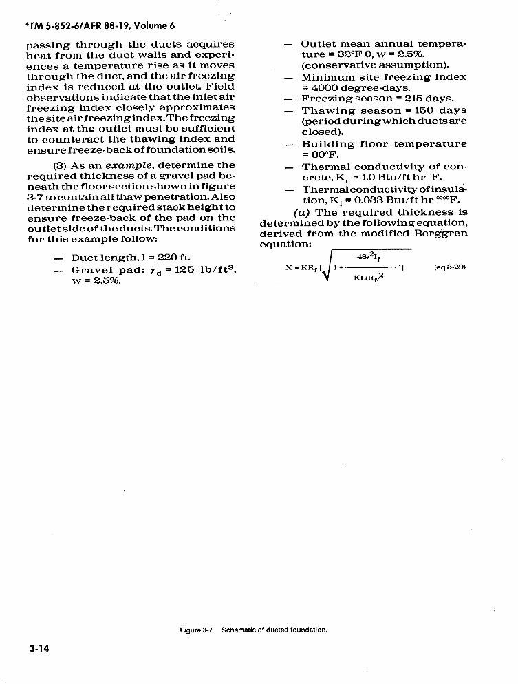
(3) As an example, determine therequired thickness of a gravel pad be-neath the floor section shownin figure3-7 to contain all thaw penetration. Alsodetermine the required stack height toensure freeze-back of the pad on theoutlet side of the ducts. The conditionsfor this example follow:

3-14

- Duct length, l = 220 ft.- Gravel pad : yd = 125 lb/ft3 ,w = 2.51 .

Figure 3-7.

Schematic of ducted foundation .

- Outlet mean annual tempera-ture = 32°F 0, w = 2.51.(conservative assumption).

- Minimum site freezing index= 4000 degree-days.

- Freezing season = 215 days.- Thawing season = 150 days

(period duringwhich ducts areclosed).

- Building floor temperature= 60°F.

- Thermal conductivity of con-crete, K. = 1.0 Btu/ft hr °F.

- Thermal conductivity ofinsula-tion, Ki = 0.033 Btu/ft hr °°°°F .

(a) The required thickness isdetermined by the followingequation,derived from the modified Berggrenequation:

48*21fX = KRf [

1 +

. 11

(eq 3-29)V

KL(Rf)2

whereK = average thermal conductivity of

gravel=1/2(0.7 + 1.0) = 0.85 Btu/ft hr °F

RT = thermal resistance of floorsystem

18 4 1212(1 .0) 12(0.033) 12(1 .0)12.5 ft2 hr °F/Btu

(eq3-30(In the computations thedead airspaceis assumed equivalent to the thermalresistance of concrete of the samethickness.)

=factor in modified Berggrenequation = 0.97 (conservativeassumption)

If= thawing indexat floorsurface= (60 - 32)(150) = 4200 degree-days

L=latent heat of gravel =144(125)(0.025 = 450 Btu/ft3

then (48)(0 .97) 2'(4200) *X- (0.85(12 .5) [ _

1 +

.11(0.85)(450)(12.5)2

- 1.1.0 ft.

(eq 3-31)(b) Thus the totalamountof heat

to be removed from the gravel pad bycold-air ventilationduring thefreezingseason with ducts open is equal to thelatent and sensible heat contained inthe thawed pad. The heat content persquare foot of pad is determined asfollows:

- Latent heat, (X)(L) = (11.0)(450)= 4950 Btu/ft2

- Sensible heat (10 percent oflatent heat, based upon ex-perience) = 495

- Total heat content:5445 Btu/ft2.

ducts will be open during thefreezing season (215 days),and theaver-age rate of heat flow from the gravelduring this season is equalto 5445/215X 24 = 1.0 Btu/ft2 hr. The average thaw-ing index at the surface of the pad is

The

LX2

(450)(11 .0)= 1420 degree-days.

4812K = 48(0.97)2(0.85)

(eq3-32)This thawing index must be com-pensated forbyan equalfreezing indexat the duct outlet on the surface of thepad to assure freeze-back.Theaverage

R

where

`TM 5-852-61AFR 88-19, Volume 6

pad surface temperature at the outletend equals the ratio

Required freezing indexLength of freezing season

1420215

=

6.6°F below32°F or 25.4°F.Theinletairduring thefreezingseasonhas an average temperature of

Air freezing index

4000Length of freezing season

215= 18.6°F below 32°F or 13.4°F.

Therefore, theaveragepermissibletem-perature rise TR along the duct is(25.4 - 13.4) = 12.0°F.

(c) The heat flowing from thefloorsurface to theductairduring thewinter is equal to the temperature difference between thefloor and duct airdivided by the thermal resistance be-tween them. The thermal resistance Ris calculated as follows:

Xe Xi 1 14Ke Ki hre (12)(1 .0)

+

4 .

+1= 12.3 hr ft2 OF/Btu(eq 3-33)(12)(0 .033) 1.0

XC = thickness of concrete (ft)Xi = thickness of insulation (ft)hre =surface transfer coefficient

between duct wall and ductair

(For practical design, hrC = 1.0 Btu/ft2hr °F and represents the combinedeffect of convection and radiation. Atmuch higher air velocities, this valuewill be slightly larger; however,usinga value of 1.0 will lead to conservativedesigns). The average heat flow be-tween the floor and inlet duct air is[(60 - 13.4)/12.3] = 3.8 Btu/ft2hr,and be- -twe.en the floor and outlet duct air is[(60 - 25.4)/12.3] = 2.8 Btu/ft2 hr. Thus

. the average rate of heat flow from thegravel pad to the duct air is 1.0 Btu/ft2hr. The total heat flow 0 to the duct airfrom the floor and gravel pad is(3.3 + 1.0) = 4.3 Btu/ft2hr.The heat flowto the duct air must equal the heatremoved by the duct air-

Heat added -heat removedOfm .60V Ad p epTR.

(eq 3-34)

3-15

*TM 5-852-6/AFR 88-19, Volume 6

Thus the average duct air velocityrequired to extract this quantity of heat(4.3 Btu/ft2 hr) is determined by theequation:

3-16

V =

ft/minute

(eq3-36)60 Ad p CpTR

wheretotal heat flow to duct air (4.3Btu/ft2 hr)

.Q

=length of duct (220 ft)

Substitution of appropriate valuesgives a required air velocity

(4.3)(220)(2.68)V=

Figure 3-8 .

Properties of dry air at atmospheric pressure.

(60)(1.68)(0.083)(0 .24)(12 .0)= 111 ft/minute.

(eq 3-36)(d) The required air flow is ob

tained by a stack or chimney effect,which is related to the stack height.The stack height is determined by theequation

m = duct spacing (2.66 ft)Ad = cross-sectional area of duct

(1.68 ft2)= density of air (0.083 lb/ft3[figure 3-10] )

lid = hV + h r (eq 3 .37)where

p ehd

H(TC . To) Inches of water5.2(T e + 460)(natural draft head)

cp = specific heat of air at constant p - density of air at average ductpressure (0.24 Btu/lb °F) temperature (lb/ft3)

TR =temperature rise in duct air e = efficiency of stack system(12°F) . This factor provides for

HTe

To

V

hf

friction losses within thechimney

= stack height (ft)= temperature of air in stack(°F)

= temperature of airsurrounding stack (°F)V 2_ (

)2 inches of water(velocity head)

= velocity of duct air (ft/minute)Is

240 ft

4000

= f- by inches of waterDe

(friction head)= friction factor(dimensionless)

= equivalent duct length (ft)= equivalent duct diameter (ft) .

used to calculate the

leDe

The techniquefriction head is

4(cross-sectional areaof duct in ft2)

4(1.58)Dc =

-perimeter of duct in ft

2 ( 18+20 + 12)12 2(eq 3-38)= 1.22 ft .

The equivalent length of the duct isequal to the actual length 1 s plus anallowance lb for bends and entry andexit. Each right-angle bend has theeffect of adding approximately 65diametersto the length of theduct,andentry and exit effects add about 10diametersforeach entry or exit. In thisexamplethetotal allowance 1b for theseeffects is [2(65 + 10) =] 150 diameters,which is added to the length of thestraight duct. The estimated length ofstraight duct Is is

5 ft

(assumed inletopen length)220 ft (length of duct beneath

floor)15 ft

(assumed stack height)

fe = ks +fb/ e m 240 + (150 X 1.22) - 423 ft.

(eq 3-39)

The friction factor f' s a function ofReynolds number NR and the ratioe/De.Areasonable absolute roughnessfactor e of the concrete duct surface is0.001 feet, based on field observations .Suggested values of e for other typesof surfaces are given in the ASHRABData and Guide Book . The effect ofminor variations in e on the friction

factor is small, as noted by examiningthe-equation below used to calculatethe friction factor f. Reynoldsnumberis obtained from the equation

V(a' + 0.25De)

whereNR -

-17,7000.49

V - average ductvelocity (ft/hr)a - shortest dimension (ft)V - kinematic viscosity

(ft2/hr at 19.4°F [fig. 3.81).The friction factor f' is obtained bysolving the equation

-0.005511+(20,000x -+-)1/311.22 17.700

-0.0285 .

(eq3-41)Therefore, the friction head is

The drafthead required to providethedesired velocity head and to overcomethe friction head is furnished by thechimney or stackeffect. Thedraftheadhd is obtained as follows:

The stack height required to producethis draft head is

5.2 hd(Tc + 460)H

(0.083)(0.80)(25.4 - 13.4)- 26 ft

wherePToToe

hd

NR

'TM 5-852-6/AFR 88-19, Volume 6

(111 X 80)(1.0 +0.25 X 1.221

f=0.0066[1 + (20,000 X -+-De NR

e423

- 0.0285 X

Xby - 9.8hv.1.22

pE(Tc - To)(5.2)(8.31x10-3)(25.4 + 460)

0.001 106

(eq 3-40)

hf- f X D X by

(eq 3-42)

(eq 3-44)

= 0.08315/ft3-25.4°F=13.4°F-8095 (found to be a reasonabledesignvaluebasedonobserva-tions over an entire season)

=8.31X103 inches of water.

347

hd - by + hf - by+9.8 by (eq 3-43)- 10.8 by

va 10.8 (-)2

4000

111a 10.8 (-)2= 8.31X10.3 inches ofwat

'TM 5-852-6/AFR 88-19, Volume 6(e) If the stack is too high for the

structure, agreaterthickness of insula-tion couldbe used. In this example, theeffectof increasing theinsulation thick-ness by one-halfwouldresult in lower-ing the stack height by five-eighths.

(f) This firstapproximated stackheight is next incorporated in the cal-culation of the length of straight duct.25, and the newly obtained fe is used torecalculate the friction head hf. By trial-and-error, the final calculated stackheight is found to be 26.5 ft .

(g) The stack height is an im-portant variable because an increasein stack height will increase the ductairflow. Circulation of air through theducts results from 1) a density dif-ference between theair inside theductand that outsidethe building,2) apres-surereductionat theoutletendattrib-utable to the stack effect, 3) a positivepressure head at the inlet end whenwind blows directly into the intakestack opening, and 4) a negative pres-sure head at the outlet when windpasses over theexhauststack opening.Draft caused by wind is highly erraticand unpredictable and should not beconsidered in design; however, thevents should be cowled to take ad-vantage of any available velocity headprovided by the wind. If sufficient aircannot be drawn through ducts bynatural draft, mechanical blowerscould be specified or considerationgiven toalternatingairflowin theducts.3-9.

Use of thermal insulating materials.An insulating layer may be used inconjunction with a non-frost-suscep-tible material to reduce the thicknessof fill required to keep freezing orthawing temperatures from pene-tratinginto anunderlying frost-suscep-tible soil. As in the example of para-graph 3-8a, the thermal resistance ofthe pavementand insulation layers areadded to obtain total resistance, andthe latent heat effect of a combinedpavement and insulation layer is as-sumed negligible . (TM5-818-2/AFM88-6, Chap.4discussesin detail thedesignof insulated pavements.) If the insu-lating material will absorb water, itsinsulating effectiveness will be re-duced considerably (as discussed in

3-18

TM5-852-4/AFM88-19, Chap. 4) . Limitedfield tests indicate that the heat-flowresistance of a Portland-cement-concrete pavement overlying a high-quality insulating layer is more compli-cated than simple addition of resist-ances, but until sufficient data areobtained for validation, treatment ofresistances in series is recommended.

a. Example. Apavement consists of14 inches of Portland-cementconcreteplaced on a 6-foot gravel base course.Frostpenetrated 3.2 feet into theunder-lyingsiltsubgrade. Determinethe thick-ness of insulation required to preventfrostpenetration into thesubgrade forthe following conditions.

- Mean annual temperature =35.3°F.

- Air freezing index =3670 degree-days

- Freezing season = 170 days- Concrete: K = 1.0 Btu/ft hr °F,

C = 0.30 Btu/ft3°F- Insulation: K = 0.024 Btu/ft hr

°F, C = 0.28 Btu/ft3 °F- Gravel base: yd = 130 lb/ft3,w=4%

- Silt subgrade: yd= 100lb/ft3,w = 10%.

Surfacefreezingindex = 0.75 X 3670 =2752 degree-days. From the knowndata

b. Trial 1. Usea2-inchlayer of insula-tion and a 6-inch concrete levelingcourse.

-Pavement section :

14 inches of concrete2 Inches of Insulation6 inches ofconcrete

levelingcourse

R

Cp

2752vs = 16.2'F (eq 3-45)

170vo 35.3 - 32.0 = 3.3'F (eq 3-46)

3.3a = =0.20 (eq 3-47)

16.2

22 inches totald 14 2=-= + +K 12x1.0 12x0.024

612x1.0

8.60 hr ft2,F/Btu (eq 3.48)(14X30) + (2X0.28) + (6X30)

2227.3 Btu/ft3 -F (eq 3-49)

The calculation appears in table 3-3and indicates that this pavement sec-tion has an excess of (2752 - 3033 =) 481degree-days to prevent frost -pene-tration into the silt subgrade.

c. Trial 2. Use a 1.5-inch layer ofinsulation and a6-inch concrete level-ing course.

-Pavement section: 14 inches ofconcrete1.5 inches of insulation6 inches ofconcrete

leveling course

21.5 inches total

Cp =

'TM 5-852-6/AFR 88-19, Volume 6 '

d 14 1.5 6RP = -=-+

+K

12X1.0

12x0.024

12x 1.06.86 hr ft2 °F/Btu

(eq 3-50)(14X30) + (1 .5X0 .28) + (6X30)

21 .5= 27.9 Btu/ft3 °F

(eq3-51)Thecalculation (see table 3-4) indicatesthat this pavement section will notprevent frost penetration into the siltsubgrade as (2752 - 2553 =) 199degree-days remain forsubgrade penetration.The 2-inch thickness of insulation istherefore required .

'TM 5-852-6/AFR 88-19, Volume 6

Table 3-3.

Insulated pavement design, no frost penetration.

Table 3-4.

Insulated pavement design, frost penetration .

3-20

4-1 . General.Radial flow of heat is considered inthermalproblems involvingthedesignof pile foundations in permafrost (TM5-852-4/AFM88-19, Chapter4),thecon-structionof utility supply lines for thetransportof waterandsewage in perma-frost areas and seasonal frost areas(TM 5-852-5/AFR88-19, Volume 5), andthe design ofartificially frozen groundfor retaining structures during con-struction. A number of the basic con-ceptsand techniquesused to calculateradial heat flow from cylindrical sur-faces are discussed below.

a. ThermalResistance. In analyzingheat flow for areas with cylindricalcross sections, the effective thicknessforradial flow fromaunit length of thecylinder is

1 r2

r2In I-, or0.367log r27r

1

1where

rI = inside wall radius (ft)r2= outside wall radius (ft) .

The thermal resistance R is equal tothe effective thickness divided by theconductivity of the material betweenthetworadii. Asan example, aconcreteconduit with a wall thickness of 6inchesandan inside diameter of 10 feetis surrounded by 4 inches of cellularglassinsulation and4feetofdrygravel.Calculate the thermal resistance be-tweenthe inside concrete wall and theouter edge of the gravel material. Thefollowing thermal conductivities aregiven:

- Concrete,K =1.00 Btu/ft hr °F.- Insulation, K = 0.033 Btu/ft hr

°F.- Gravel, K = 1.5 Btu/ft hr °F.

Let (see fig. 4-1 for values of rI - r4)rI=radius to inner wall of conduitr2=radius to outer wall of concrete

CHAPTER 4

TWO-DIMENSIONAL RADIAL HEAT FLOW

1 r4+ - log -K3-4 r3

0.352

*TM 5-852-6/AFR 88-19, Volume 6

r3= radius to outer edge of insula-tion

r4= radius to outer edge of gravelK1-2

thermalconductivity ofconcreteK2-3 = thermal conductivity of insula-

tionK3-4 =thermal conductivity of gravel.

1 r2 1 r3R-0.367( - log

+

- log

(eq 4-1)'1 -2 r K2-3 r2

1 5.5 1 5.83 1 9.83=0.367 ( - log - + - log _+_109 -+)1.0 5.0 0.033 5.5 1.5 5.83-0.367 (0.041 + 0.767 + 0.151) -0.352 ft.2 hr °F/Btu.

If the temperature in the conduitwere45°F and the temperature at the outer,face of the gravel were 35°F, the heatflow per linear foot of conduit wouldequal

(45 - 35) - 28.4 Btu/hr.

(eq 4-2)

b. Temperature field surroundinga cylinder. Thesudden or step changein surface temperature discussed forsemi-infinite slabs in paragraph 3-6ahas application to heat-flow problemsassociated with pile foudations inpermafrost. A mathematical solutiopis available for the problem where the .surface temperature of a cylinder issuddenly changed from the uniformtemperature of the surroundingmedium, as long as there is no phasechange. Figure 4-2 is used to determinethe temperature T ata distance r fromthecenter ofacylinder of radius rhat atime tafter the surface temperature ofthe cylinder is changed from To to T8.ThetemperatureTorepresents theuni-form temperature of themediumpriorto the sudden change in surfacetemperature.

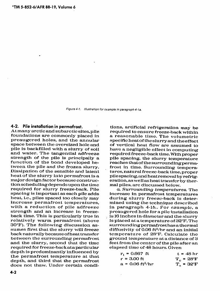
'TM 5-852-6/AFR 88-19, Volume 6

4-2 .

Pile installation in permafrost.Atmany arctic and subarctic sites, pilefoundations are commonly placed inpreaugered holes, and the annularspace between the oversized hole andpile is backfilled with a slurry of soiland water. The tangential adfreezestrength of the pile is principally afunction of the bond developed be-tween the pile and the frozen slurry .Dissipation of the sensible and latentheat of the slurry into permafrost is amajordesign factor because construc-tion schedulingdependsuponthe timerequired for slurry freeze-back . Pilespacing is important as each pile addsheat, i.e ., piles spaced too closely mayincrease permafrost temperatures,with a reduction of pile adfreezestrength and an increase in freeze-back time. This is particularly true inrelatively warm permafrost (above30°F). The following discussion as-sumes first that the slurry will freezeback naturally because of heattransferbetween the surrounding permafrostand the slurry, second that the timerequired for freeze-back at a particulardepth is predominantly influenced bythe permafrost temperature at thatdepth, and third that the permafrostdoes not thaw. Under certain condi-4-2

Figure 4-1 .

Illustration for example in paragraph 4-1a .

tions, artificial refrigeration may berequired to ensure freeze-back withina reasonable time . The volumetricspecific heat of the slurry and the effectof vertical heat flow are assumed tohave a negligible effect in computingrequired freeze-back time. With properpile spacing, the slurry temperaturereaches thatof the surroundingperma-frost in time. Surrounding tempera-tures, natural freeze-back time, properpile spacing, andheatremoval by refrig-eration, as well as heat transferby ther-mal piles, are discussed below.

a. Surrounding temperatures. Theincrease in permafrost temperaturesduring slurry freeze-back is determined using the technique describedin paragraph 4-1b. . For example, apreaugered hole for a pile installationis 16 inches in diameter and the slurryis placed at a temperature of 32°F. Thesurrounding permafrost hasa thermaldiffusivity of 0.06 ft2/hr and an initialtemperature of 28°F . Calculate theground temperature at a distance of 3feet from the center of the pile after anelapsed time of 48 hours . Given

rl = 0.667 ft t = 48 hrr = 3.00 ft To = 28°Fa = 0.06 ft2/hr TS = 32°F

Figure 4-2. Temperature around a cylinder having received a step change in temperature.

therefore,

From figure 4-2,

r 10.667

T - To~ -

= 0.39

(eq 4.3)

= -..-V

(0.06)(48)

TS' TO

r 3.00- _ - = 4.60 .

(eq 4-4)r l 0.667

"TM 5-852-6/AFR 88-19, Volume 6

(eq 4-6)

T = 0.18 (TS - To)+To = 0.18 (32-28)+28

= 28.7°F .

(eq 4-6)

4-3

'TM 5-852-6/AFR 88-19, Volume 6

This technique is also used to predictthe increase in permafrost temperatureduring slurry freeze-back. Since it as-sumes aconstant surface temperaturefor a cylinder, it is applicable only tothe time offreeze-back . After the slurryhas frozen, the permafrost temperaturedecreases and the model is not valid.

b. Natural freeze-back time. Thisheat transfer problem assumes a slur-ried pile to be a finite heat source inside

4-4Figure 4-3.

General solution of slurry freeze-back.

a semi-infinite medium, with asuddenlyapplied constant temperature source(32°F) that dissipates radially intofrozen ground ofknown initial tempera-ture . The general solution for thenatural freeze-back problem, basedupon the latent heat content of theslurry, is shown in figure 4-3.

(1) For example, calculate the timerequired to freeze back a 12 .5-inchdiameter timber pile placed in an 18-

inch hole preaugered in permafrostand backfilled with a slurry for thefollowing conditions :

- Permafrost:

Silty sandInitial temperature - 27°FDry unit weight = 941b/ft3Water content - 259 .

- Slurry backfill:

Silt, waterPlacement tempera-ture - 33.5°FDry unit weight - 72 ib/ft3Water content - 45%.

In figure 2-3, the thermal conductivityof the permafrost is determined to be1.1 Btu/ft hr°F. The volumetric heatcapa-city is calculated to be

[94 (0.17 + 0.525100 )] - 27.7 Btu/ft3 °17

(eq4-7)

and the thermal diffusivity to be1.127.7

Thevolumetric latentheatof theslurryis

(144 X 72 X 0.45) - 4970 Btu/ft3 °17

(eq4-9)and the latent heat per linear foot ofbackfill is

n[ 4 (1 .52 .1.042)] 4970 -4280 Btu.

(eq4.10)

Whenfigure 4-3 is entered with avalueof

Cr2At

then,at

- 0.0397 ft2/hr.

(eq4-8)

- .12.4.r22

(27.7)(0.752)(5)1 .55

(eq4.11)

(eq 4-12)

The time required to freeze back theslurry backfill is

12 .4 X 0.752- 179 hoursor about0.0397

7.3days.

(eq4-13)At this time the slurry temperature is32°F. Subsequent to freeze-back, thetemperature of the slurry will continueto decrease and will approach thepermafrost temperature . Ninety per-cent of the temperature difference ; willdisappear in about twice the time re-quired for freeze-back to 32°F. In thisexample, after a period of [7.3 + (2X 7.3) =122 days, the slurrytemperaturewould be approximately [32 - 0.90 (32 -27) =1 27.5°F . The time (22 days) should

'TM 5-852-6/AFR 88-19, Volume 6

be increased by 50 percent to permitan element of safety in the design.(Note: the sensible heat introduced bythe pile and slurry was negligible incomparison to the latent heat intro-duced by the slurry and was not con-sidered in calculations.)

(2) Permafrosttemperature varia-tions with depth, as discussed in TM5-852-4/AFM 88-19, Chap. 4, should beconsidered in calculating freeze-backtime. Figure 4-4 illustrates the effectof permafrost temperature on freeze-back for the above example. Sinceheatinput is governed principally by thelatentheat ofslurry backfill, which is afunction of slurry volume, moisturecontent and dry unit weight, a familyof curves relating volumetric latentheat of slurry, permafrost tempera-tures and freeze-back time may be de-veloped for a specific site to account

Figure 4-4.

Specific solution of slurry freeze-back

4-5

*TM 5-852-6/AFR 88-19, Volume 6

for varying pile shapesandpreaugeredhole diameters. To minimize the heatintroduced by the slurry, the watercontent should be the minimum re-quired for complete saturation . Thiscanbe bestaccomplished by backfillingwith the highest dry unit weight mate-rial that can be processed and placed,i.e., a well-graded concrete sand with a6-inch slump.

c. Pile Spacing. The effect of pilespacing on the overall rise of perma-frost temperature resultingfrom installation of piles in preaugered holes isfound by equating the latent heat ofslurry backfill with the allowable sen-sible heat (temperature) rise of the sur-rounding permafrost . For example,calculate the minimum allowable pilespacing in the preceding example sothat the permafrost temperature willnot rise above 31°F.Thefollowingequa-tion, equating the latent heat of theslurry to the change of sensible heat ina permafrostprism of side S, is used todetermine the pile spacing:

s =

(nr2) +

Q

(eq4-14)C AT

whereS

= grid pile spacing (ft)r2 = radius of augered hole (ft)Q

= latent heat of slurry per lineal foot(Btu/ft)

C = volumetric heatcapacity ofperma-frost (Btu/ft3 °F)

AT= temperature rise of permafrost(°F) .

Substitution ofappropriate values fromthe aboveexampleand amaximum allow-able permafrost temperature rise ATof 4°F give aminimum pile spacing S of

4280(3.14)(0.75)2 +

=6.4 ft.

(eq 4-15)(27.7)(4)This spacing may not keep local tem-perature from rising to more than 31°F;however, itwill keep the entire mass ofpermafrost from reaching that tempera-ture.

(1) Numerical analysis ofanumberof pile installations indicates that pilespacing should be at least five diameters of the drill hole size . A plot, similarto that shown in figure 4-4, may beprepared to relate pile spacing and

4-6

permafrost temperature rise for thevolumetric latent heat of the slurrybackfill introduced into the drill hole.A family of curves may be developed toaccount for variation of slurry volumet-ric latent heat.

(2) In this example the slurry back-fill was placed ata temperature slightlyabove freezing (33.5°F) and, theoretically, the sensible heat of the slurryshould be considered . The volumetriccapacity of the unfrozen slurry was[72(0.17 + 1.0 X 0.45) _] 44.6 Btu/ft3 °F,and with a temperature difference of(33.5 - 32 =) 1.5°F, this represents asensible heat of (1.5 X 44.6 =) 67 Btu/ft3.A comparison of this quantity with thevolumetric latent heat of the slurry(4670 Btu/ft3) shows that its heat maybe considered negligible, as long as itnear the freezing point.

d. Artificialfreeze-back time. Ifper-mafrost is temperatures are marginal,it may be necessary to refrigerate thepile to accelerate slurry freeze-backtime and to have refrigerationavailableif permafrost temperatures rise afterconstruction. The following exampleshows calculations required to deter-mine theamount of heat to be extractedfrom the ground. The average volumeof slurry backfill for a group of piles is31 cubic feet each. The slurry is placedat a naverage temperature of 48°F andmust be frozen to 23°F. A silt-waterslurry of SO lb/ft3 dry weight and 40percent water content is used as back-fill material, and an available refrigera-tion unit is capable of removing225,000Btu/hr. Calculate the length of timerequired to freeze back a cluster of 20piles .

-Volumetric latent heat of back-fill :

L = (1-14 X 80 X 0.40) = 4600 Btu/ft3.

(eq4-16)-Volumetric heat capacity of

frozen backfill :Cf = 80 (0.17 + (0.5X0.4)) = 29.6 Btu/ft3 °F .

(eq 4-17)-Volumetric heat capacity of un-

frozen backfill :Cu = 80 [0.17 +(1.0X0.4)) = 46.6 Btu/ft3 °F .

(eq 4-18)-Heatrequired to lower the slurry

temperature to the freezing point-46.6 X 31 (48 - 32) = 22,618 Btu/pile .

(eq4-19)-Heat required to freeze slurry:31 X 4600 = 142,600 Btu/pile .

(eq 4-20)

-Heat required to lower theslurry temperature from the freezingpoint to 23°F;

29.6 X 31 (32 - 23) = 8258 Btu/pile .

(eq 4-21)-Total heat to be removed from

the slurry :20 (22,600 + 142,700 + 8200) = 3,470,000 Btu.

(eq 4-22)-Time required for artificial

freeze-back, excluding allowances forsystem losses:

3,470,000/225,000 - 15.5 hours.

(eq4-23)e. Meat transfer by thermal piles.

Artificial freeze-back may be accom-plished also by use oftwotypes ofself-refrigerated heat exchangers : a single-phase liquid-convection heat transferdevice and a two-phase boiling-liquidand vapor convection heat transferdevice. TM 5-852-4/AFM 88-19, Chapter4 presents heat transfer rates for thetwo-phase system . There are few heattransfer field data available for thesingle-phase system.

4-3. Utility distribution systems in frozenground.General considerations for the designof utility systems in cold regions aregiven inTM5-852-5/AFR 88-19, Volume5.

a. Burying water pipes in frozenground. Water pipes that are buried infrozenground maybekept from freezing by any one of the followingmethods: 1) placing the waterline in aninsulated utilidor, which is a contin-uousclosed conduit with all lines, suchas water, sewage and steamlines, in-stalled away from direct contact withfrozen ground, 2) providing a suf-ficient flow velocity such that the watertemperature at the terminusofthe pipe-line does not reach the freezing pointor 3) heating the water at the intake orat intermediate stations along the line .A layer of insulation around a pipelinewill retard, but not prevent, freezing ofstanding water in a pipe. The thermalanalysis of a pipeline buried in frozenground is complicated by the changingthermal properties, ice content, sea-sonal and diurnal changes of tempera-ture and the intermittent water flow.Some calculation techniques applic-able to the problem of buried utilitiesare presented below for standing andfor flowing water. Additional tech-

niques are presented in TM 5-852-5/AFR 88-19, Volume 5.

b. Freezing of standing water in aburied pipe. Problems with freezeupof stationary water must take intoaccount the initial time required tolower the water temperature to thefreezing point and the amount of timerequired to form an annulus of ice inthe pipe. In most instances the dangerpoint is reached when water begins tofreeze .

(1) The time required to lower thetemperature of nonflowing water inan insulated pipe to the freezing pointis given by the equation

t=

*TM 5-852-6/AFR 88-19, Volume 6

31.2 ri TN,-Ts(r' In rp )In-K,

32-Ts (eq 4-24)

wheret

=time (hr)Ki = thermal conductivity of in-

sulation (Btu/ft hr °F)rp = radius of pipe (ft)r i = radius to outer edge ofinsula-

tion (ft)T N, = initial water temperature (°F)Ts = temperature ofsurrounding

soil (°F) .For example, a 12-inch diameter ironpipe containingwater at42°F is buriedin 28°F soil . Determine the time re-quired to lower the water temperatureto 32°F if the pipe is insulated with 3Inches of cellular glass (K i = 0.033Btu/ft hr°F) .

31.2 -

_ 0.75

42-28t - - (0.502 In - ) in -- 120hours (5 days)

0.033

0.50

32-28

eq4-25

(2) Once the water temperaturehas been lowered to the freezing point,ice begins to form in an annular ringinside the pipe. The following assump-tions are made to solve this problem:

-The water is initially at 32°F.-Theheatreleasedbythe freezing

of water does not affect the sur-rounding ground temperatures .

-The volumetric heat capacity ofthe ice may be ignored .

-The thermal resistance of thepipe wall is negligible.The solution predicts the time requiredto form an annulus of ice around theinner wall of the pipe. Knowledge ofpipe radius, insulation thickness and

4-7

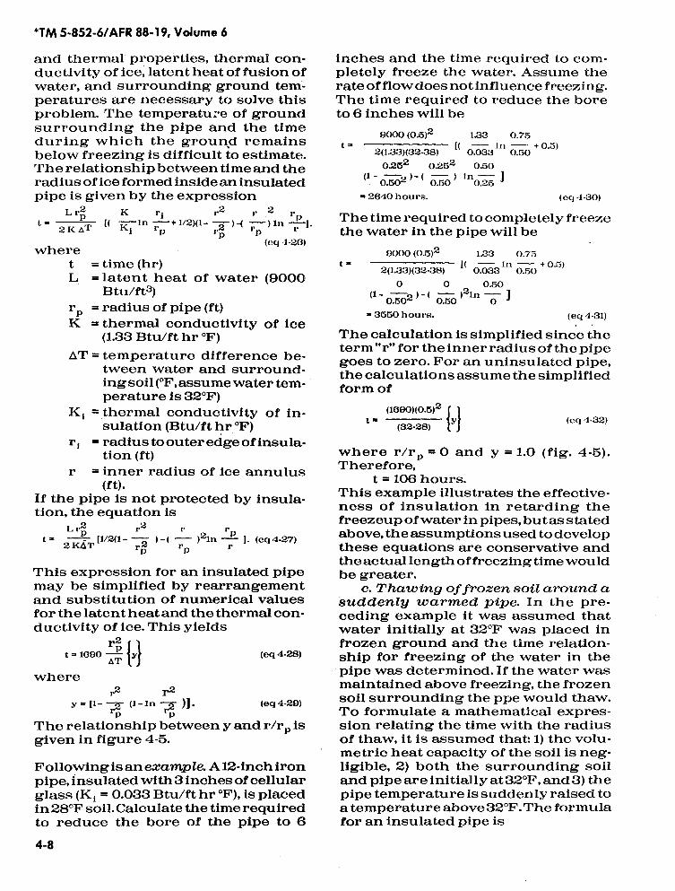
'TM 5-852-6/AFR 88-19, Volume 6

and thermal properties, thermal con-ductivity of ice, latent heat of fusion ofwater, and surrounding ground tem-peratures are necessary to solve thisproblem. The temperatuze of groundsurrounding the pipe and the timeduring which the ground remainsbelow freezing is difficult to estimate.The relationship between timeand theradius of ice formed inside an insulatedpipe is given by the expression

L r2K

rir 2r

2

rt= T [( -1n-+1/2)(1--r2 )-( r )In P-].

2K0 i p p p(eq 4-26)

wheret

= time (hr)L = latent heat of water (9000

Btu/ft3)rp = radius of pipe (ft)K = thermal conductivity of ice

(1.33 Btu/ft hr °F)AT = temperature difference be-

tween water and surround-ingsoil (°F, assume water tem-perature is 32°F)

K i = .thermal conductivity of in-sulation (Btu/ft hr °F)

ri =radius to outer edgeof insula-tion (ft)

r

=inner radius of ice annulus(ft) .

If the pipe is not protected by insula-tion, the equation is

t

This expression for an insulated pipemay be simplified by rearrangementand substitution of numerical valuesfor the latent heat and the thermal con-ductivity of ice. This yields

The relationship between y and r/rp isgiven in figure 4-5.

Following is anexample. A12-inch ironpipe, insulated with 3 inches of cellularglass (Ki = 0.033 Btu/ft hr °F), is placedin 28°F soil. Calculate the time requiredto reduce the bore of the pipe to 64-8

Lr2

r2 r r=

KIT[1/2(1-

2 ) -(r

)21n

P 1 . (eq 4-27)2

rp p

inches and the time required to com-pletely freeze the water. Assume therate of flow does not influence freezing.The time required to reduce the boreto 6 inches will be

t=

t

9000 (0.5)2

1.33

0.75r

2(1.33)(32-38)

[( 0.0331n 0.50 +0..~)

0.252 0.252 0.501_

6.502)- ( 0.50 ) in0.25- 2640 hours.

(eq 4-30)

The time required to completely freezethe water in the pipe will be

9000 (0 .5)2

1.33

0.752(1.33)(32-38)

[( 0.033 1I~ 0.50 + 0.5)

O O 0.50(1-0

.502)-( 0.50 )21°o l

- 3550 hours.

(eq4-31)

The calculation is simplified since theterm"r" for the inner radius of the pipegoes to zero. For an uninsulated pipe,the calculations assumethe simplifiedform of

(1690)(0.5)2

~Y~(32 28)

where r/r p = O andTherefore,

t = 106 hours.This example illustrates the effective-ness of insulation in retarding thefreezeup of water in pipes, but as statedabove, the assumptions used to developthese equations are conservative andthe actual length offreezing timewouldbe greater .

e. Thawing offrozen soil around asuddenly warmed pipe . In the pre-ceding example it was assumed thatwater initially at 32°F was placed infrozen ground and the time relation-ship for freezing of the water in thepipe was determined . If the water wasmaintained above freezing, the frozensoil surrounding the ppe would thaw.To formulate a mathematical expres-sion relating the time with the radiusof thaw, it is assumed that: 1) the volu-metric heat capacity of the soil is neg-ligible, 2) both the surrounding soiland pipe are initially at 32°F, and 3) thepipe temperature is suddenly raised toa temperature above 32°F. The formulafor an insulated pipe is

y = 1 .0 (fig . 4-5) .

rt = 1690 QT jyj (eq 4-28)

wherer2 r2

Y = [1-x2

(1-1n A- (eq 4-29)p p

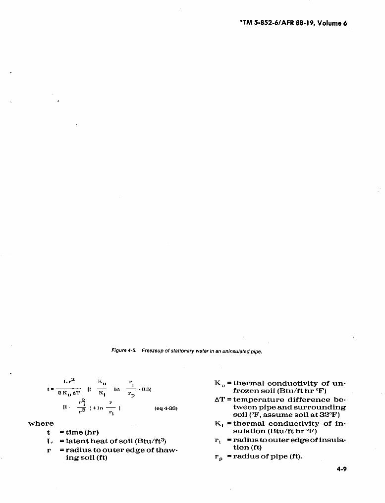
'TM 5-852-6/AFR 88-19, Volume 6

4-9

Figure 4-5. Freezeup of stationary water in an uninsulated pipe .

Lr2 KU ri KU = thermal conductivity of un-In2 KU pT V

Ki rP.0.5) frozen soil (Btu/fthr °F)

r2 r QT = temperature difference be-[I -

r2 )+'n 1 (e9 4-33) tween pipeand surroundingi soil (°F, assume soil at 32°F)

where Ki = thermal conductivity of in-t = time (hr) sulation (Btu/ft hr °F)L = latent heat of soil (Btu/ft3) ri =radiusto outeredge ofinsula-r = radius to outer edge of thaw- tion (ft)

ingsoil (ft) rP = radius of pipe (ft) .

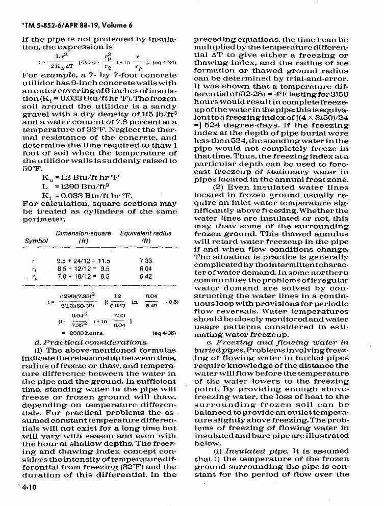
*TM 5-852-6/AFR 88-19, Volume 6

If the pipe is not protected by insula-tion, the expression is

L r2r2rt

4T

[-0.5 (1 -

r

) + In . 1 . (eq 4-34)2I{u

2

r pFor example, a 7- by 7-foot concreteutilidor has 9-inch concrete walls withan outer covering of 6 inches ofinsula-tion (K i = 0.033 Btu/ft hr °F). The frozensoil around the utilidor is a sandygravel with a dry density of 115 lb/fOand a water content of 7.8 percent at atemperature of 32°F. Neglect the ther-mal resistance of the concrete, anddetermine the time required to thaw 1foot of soil when the temperature ofthe utilidor walls is suddenly raised to50°F.

Ku =1.2 Btu/ft hr °FL =1290 Btu/ft3K i = 0.033 Btu/ft hr °F.

For calculation, square sections maybe treated as cylinders of the sameperimeter.

" 4-10

t(1290)(7.33)2 1.2 6.04

U2(1.2)(50-32) 0.033 5.42

6.042 7.33

7.332

) +In

64

In .0.5)

= 2060 hours .

(eq 4-35)

d. Practical considerations.(1) The above-mentioned formulas

indicate the relationship between time,radius of freeze or thaw, and temperature difference between the water inthe pipe and the ground. In sufficienttime, standing water in the pipe willfreeze or frozen ground will thaw,depending on temperature differen-tials. For practical problems the as-sumed constant temperature differen-tials will not exist for a long time butwill vary with season and even withthe hour at shallow depths. The freez-ing and thawing index concept con-siders the intensity of temperature dif-ferential from freezing (32°F) and theduration of this differential . In the

preceding equations, the time t can bemultiplied by the temperature differen-tial AT to give either a freezing orthawing index, and the radius of iceformation or thawed ground radiuscan be determined by trial-and-error .It was shown that a temperature dif-ferential of(32-28) = 4°F lasting for 3150hourswould result in complete freeze-up ofthe water in thepipe; this is equiva-lent to a freezing index of [(4 X 3150)/24=1 524 degree-days . If the freezingindex at the depth of pipe burial wereless than 524, the standing water in thepipe would not completely freeze inthat time. Thus, the freezing index at aparticular depth can be used to fore-cast freezeup of stationary water inpipes located in the annual frost zone.

(2) Even insulated water lineslocated in frozen ground usually re-quire an inlet water temperature significantly above freezing. Whether thewater lines are insulated or not, thismay thaw some of the surroundingfrozen ground. This thawed annuluswill retard water freezeup in the pipeif and when flow conditions change.The situation is practice is generallycomplicated bythe intermittentcharac-ter of water demand. Insomenortherncommunities the problems of irregularwater demand are solved by con-structing the water lines in a contin-uousloop with provisions for periodicflow reversals . Water temperaturesshould be closely monitored and waterusage patterns considered in esti-mating water freezeup .

e. Freezing and flowing water inburied pipes.Problems involvingfreez-ing of flowing water in buried pipesrequire knowledge of the distance thewater will flow before the temperatureof the water lowers to the freezingpoint. By providing enough above-freezing water, the loss of heat to thesurrounding frozen soil can bebalanced to provide an outlet tempera-ture slightly above freezing. The prob-lems of freezing of flowing water ininsulated and bare pipe are illustratedbelow.

(1) Insulated pipe. It is assumedthat 1) the temperature of the frozenground surrounding the pipe is constant for the period of flow over the

SymbolDimension-square

ONEquivalent radius

(ft)

r 9.5+24/12=11 .5 7.33r ; 8 .5 + 12/12 = 9.5 6.04rp 7.0 + 18/12 = 8.5 5.42

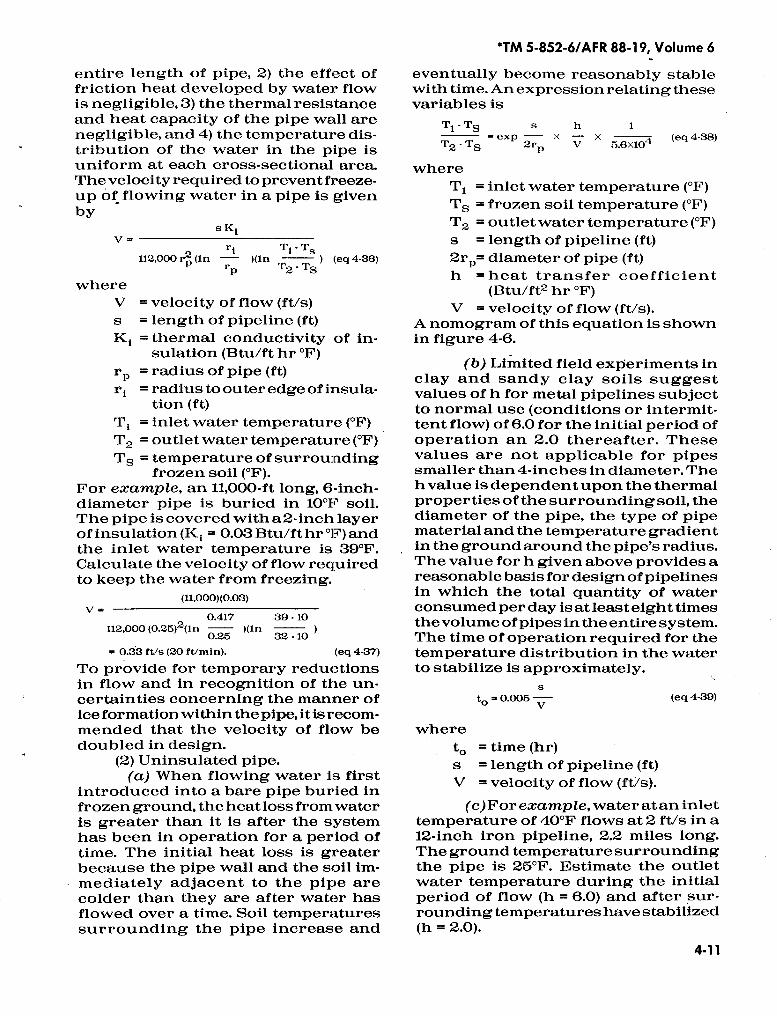
entire length of pipe, 2) the effect offriction heat developed by water flowis negligible, 3) the thermal resistanceand heat capacity of the pipe wall arenegligible, and 4) the temperature dis-tribution of the water in the pipe isuniform at each cross-sectional area.The velocity required to prevent freeze-up of flowing water in a pipe is givenby -

v

= 0.33 ft/s (20 ft/min).

s Kiri TI-Ts

112,000 r2 (In

-

)(InT2 -

T

)

(eq 4-36)p

Swhere

V

= velocity of flow (ft/s)s

=length of pipeline (ft)= thermal conductivity of in-sulation (Btu/ft hr °F)

= radius of pipe (ft)= radius to outer edge ofinsula-

rnri

tion (ft)Ti = inlet water temperature (°F)T2 =outletwater temperature (°F)Ts = temperature of surrounding

frozen soil (°F) .For example, an 11,000-ft long, 6-Inch-diameter pipe is buried in 10°Fr soil.The pipe is covered with a2-inch layerof insulation (Ki = 0.03 Btu/ft hr °F) andthe inlet water temperature is 39°F.Calculate the velocity of flow requiredto keep the water from freezing.

(11,000)(0.03)v= 0.417 39-10

112,000 (0 .25)2(ln 0,25

)(In

32-10 )(eq 4-37)

To provide for temporary reductionsin flow and in recognition of the un-certainties concerning the manner ofice formation within the pipe, it is recom-mended that the velocity of flow bedoubled in design.

(2) Uninsulated pipe.(a) When flowing water is first

introduced into a bare pipe buried infrozen ground, the heatloss from wateris greater than it is after the systemhas been in operation for a period oftime. The initial heat loss is greaterbecause the pipe wall and the soil im-mediately adjacent to the pipe arecolder than they are after water hasflowed over a time. Soil temperaturessurrounding the pipe increase and

*TM 5-852-6/AFR 88-19, Volume 6

eventually become reasonably stablewith time. An expression relating thesevariables is

T1, TSs

h

1T2 -

TS= exp

2rpX

v X 5.6X104

(eq4-38)

whereTl = inlet water temperature (°F)Ts = frozen soil temperature (°F)T2 =outletwater temperature (°F)s

=length of pipeline (ft)2rp diameter of pipe (ft)h =heat transfer coefficient

(Btu/ft2 hr °F)V

=velocity of flow (ft/s) .A nomogram of this equation is shownin figure 4-6.

(b) Limited field experiments inclay and sandy clay soils suggestvalues ofh for metal pipelines subjectto normal use (conditions or intermit-tent flow) of 6.0 for the initial period ofoperation an 2 .0 thereafter. Thesevalues are not applicable for pipessmaller than 4-inches in diameter. Thehvalue is dependentuponthe thermalproperties of the surrounding soil, thediameter of the pipe, the type of pipematerial and the temperature gradientin the groundaround the pipe's radius.The value for h given above provides areasonable basis for design ofpipelinesin which the total quantity of waterconsumedperday is at least eight timesthe volume ofpipes in the entire system.The time of operation required for thetemperature distribution in the waterto stabilize is approximately .

Sto = 0.005v

(eq 4-39)

whereto

= time (hr)s

=length of pipeline (ft)V

= velocity of flow (ft/s) .(c)For example, water atan inlet

temperature of 40°F flows at 2 ft/s in a12-inch iron pipeline, 2.2 miles long.Thegroundtemperature surroundingthe pipe is 25°F. Estimate the outletwater temperature during the initialperiod of flow (h = 6.0) and after sur-rounding temperatures have stabilized(h = 2.0) .

4-1 1

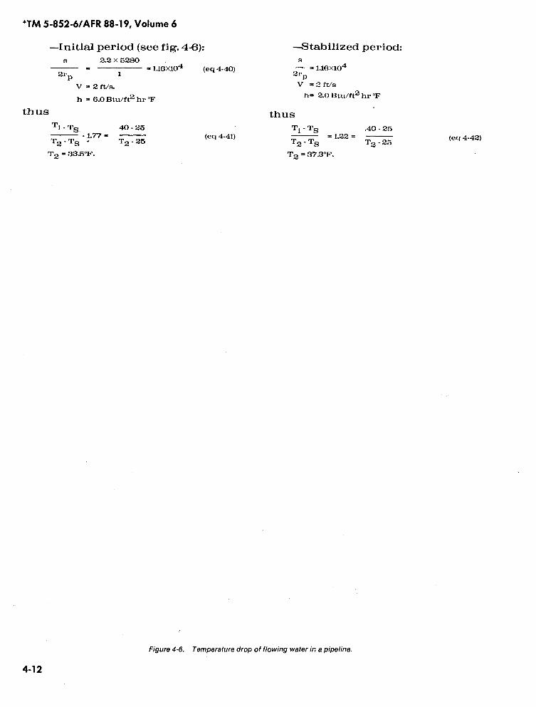
*TM 5-852-6/AFR 88-19, Volume 6

-Initial period (see fig. 4-6) :

-Stabilized period:

thus

4- 12

s

2.2 X 5280

s

2:-

=

1

= 1.16X .104(eq4-40)

2r = 1.16X104P

AV = 2 ft/s.

V

='.3 ft/s

h = 6.0 Btu/ft2 hr °F h- 2.0 Btu/ft2 hr °F

thusT1 - TS,

40-25

Tl - TS

.40-25T

_11" =

T

(eq 4-41)

T

= 1.22 =2 -TS

2-25

T2'

S

T2- 25T2 - 33.5°F .

T2 -37.3°F .

Figure 4-6.

Temperature drop of flowing water in a pipeline.

(eq 4-42)

To operate on the safe side, the outlettemperature T2 should remain at orabove 35°F. The calculated initial watertemperature of 33.5°F would be con-sidered unsafeand either the flow velo-city should be increased to approxi-mately 3 ft/s or the inletwater tempera-ture should be raised to about 43°F.These- precautions would be neededonly for an initial period, i.e .,

s 11 .600to =

0.005V= 0.005

2= approximately 29 hours.

(eq 4-43)

f. Design considerations . The cal-culation techniques presented aboveindicate the principal factors to be con-sidered in design of water distributionlines placed in frozenground . Theuseofthese techniques together with recog-nition of the complexities of actual in-pipe ice formation and sound engi-neering judgmentprovides a basis fordesign ofpipelines in areas of seasonalfrostand permafrost. Changing the sur-face cover over an installed pipelinewill affect the distribution of tempera-tures with depth and may result indepressing the temperatures adjacentto the pipe. This is particularly true ifanatural vegetative cover is stripped andreplaced bya snow-free pavement .Theinfluence of new construction abovean existing pipeline may require achange in operating procedures forthe system, such as an increase in thevelocity or flow or additional heatingat the inlet.4-4. Discussion of multidimensional heatflow.

a. The relatively simple analyticaltechniques discussed in this manualare not always sufficient for considering the concurrent thermal effects ofmultidimensional temperature changeand soil water phase transformation .The one-dimensional and radial heat-flow computation techniques pres-ented in this manual were based onfield observations and the use ofreason-able simplifyingassumptions. The tech-niques are intended to facilitate ana-

*TM 5-852-6/AFR 88-19, Volume 6

lysis and to promote adequate design.The assumptions involved and tech-nique limitations have been em-phasized .

b. Heat flow beneath heated struc-tures is multidimensional because ofthe finite boundaries of such structures.The ground surface temperatureadjacent to the south side of the build-ing is generally higher than that onthe north side, and the ground surfacetemperature on the west side is gen-erally higher than on the east side; inaddition to this influence, the three-dimensional temperature distributionbeneath the building will be affectedby the plan dimensions of the floor .Three-dimensional solutions are avail-able to the problem of heat flow inhomogeneous materials beneath thesurface of a heated finite area sur-rounded by an infinite area subject toadissimilar surface temperature condi-tion; however, the solutions consideronly the effects of temperature changeandnotthe effects of phase transforma-tions. Such solutions tend to be rathercomplex and unwieldy, and theirneglect of latent heat generally resultsin an over-estimation of the depth offreeze or thaw. The magnitude of thisover-estimation is dependent on thequantity of moisture in the frozen orthawed soil .

c . The example given in paragraph3-8a for calculating the depth of thawbeneath a heated slab-on-grade building considered only one-dimensionalvertical heat flow and excluded lateralheat flow from the soil beneath the,building to the surrounding soil massin the winter . The amount of lateralheat flowwoulddepend on the buildingdimensions and the wintertime soil tem-perature gradient. Slab-on-grade,heated structures usually preventfrost penetration under the center ofthe building and result in a thaw bulbin the foundation soil that may causepermafrostdegradation with time.Thistype of construction is discussed inTM 5-852-4/AFM 88-19, Chapter 4.

4-1 3

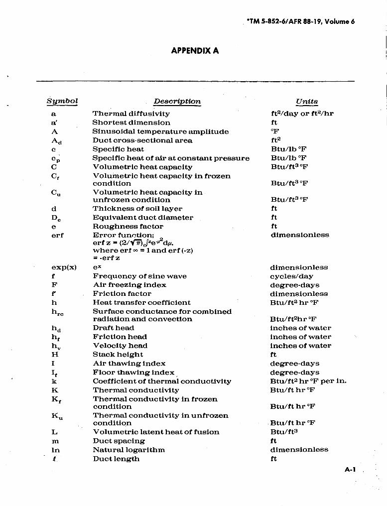
APPENDIX A

'TM 5-852-6/AFR 88-19, Volume 6

Sumbot Description Unitsa Thermal diffusivity ft2/day or ft2/hra' Shortest dimension ftA Sinusoidal temperature amplitude °FAd Duct cross-sectional area ft2c Specific heat Btu/lb °F

Specific heat of air at constant pressure Btu/lb °FC Volumetric heat capacity Btu/ft3 °FC f Volumetric heat capacity in frozen

condition Btu/ft3 °FCu Volumetric heat capacity in

unfrozen condition Btu/ft3 °Fd Thickness of soil layer ftDe Equivalent duct diameter fte Roughness factor fterf Error function; dimensionless

erf z = (2/Y77_r)a(ze-Y2dp,where ert = 1 and. erf (-z)= -erf z

exp(x) ex dimensionlessf Frequency of sine wave cycles/dayF Air freezing index degree-daysf. Friction factor dimensionlessh Heat transfer coefficient Btu/ft2 hr °Fhre Surface conductance for combined

radiation and convection Btu/ft2hr °Fhd Draft head inches of waterhf Friction head inches of waterhV Velocity head inches of waterH Stack height ftI Air thawingindex degree-daysif Floor thawing Index,, degree-daysk Coefficient of thermal conductivity Btu/ft2 hr °F per in.K Thermal conductivity Btu/fthr °FK f Thermal conductivity in frozen

condition Btu/ft hr °FKu Thermal conductivity in unfrozen

condition Btu/ft hr °FL Volumetric latent heat of fusion Btu/ft3m Duct spacing ftIn Natural logarithm dimensionlessf . Duct length ft

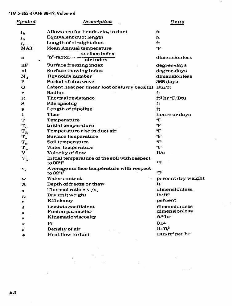
'TM 5-852-6/AFR 88-19, Volume 6

symbol Description Units

1b Allowance for bends,, etc., in duct ftle Equivalent duct length ftIs Length of straight duct ftMAT Mean Annual temperature °F

surface indexn "n"-factor = air index dimensionlessnF Surface freezing index degree-daysnI Surface thawing index degree-daysNR Reynolds number dimensionlessP Period of sine wave 366 daysQ Latent heat per linear foot of slurry baekfill Btu/ftr Radius ftR Thermal resistance ft2 hr °F/BtuS Pile spacing fts Length of pipeline ftt Time hours or daysT Temperature °FTo Initial temperature °FTR Temperature rise in duct air °FTS Surface temperature °FTs Soil temperature °FTw Water temperature °FV Velocity of flow ft/sVo Initial temperature of the soil with respect

to 32°F °Fvs Average surface temperature with respect

to 32°F °Fw Water content percent dry weightX Depth of freeze or thaw fta Thermal ratio - vo/v$ dimensionlessYd Dry unit weight lb/ft3s Efficiency percent

Lambdacoefficient dimensionlessu Fusion parameter dimensionlessv Kinematic viscosity ft2/hr

Pi 3.14P Density of air lb/ft3

Heat flow to duct Btu/ft2 per hr

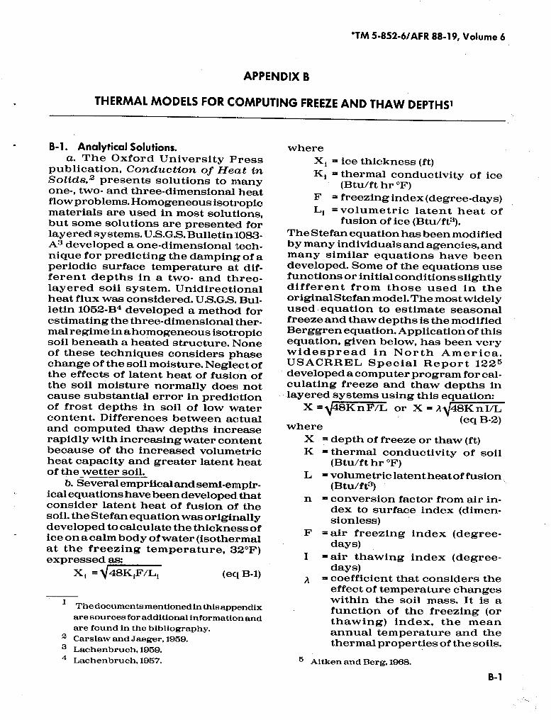
APPENDIX B

THERMAL MODELS FOR COMPUTING FREEZE AND THAW DEPTHSI

B-1 .

Analytical Solutions.a. The Oxford University Press

publication, Conduction of Heat inSolids,2 presents solutions to manyone-, two- and three-dimensional heatflow problems. Homogeneous isotropicmaterials are used in most solutions,but some solutions are presented forlayered systems.U.S.G.S . Bulletin 1083-A3 developed a one-dimensional tech-nique for predicting the damping of aperiodic surface temperature at dif-ferent depths in a two- and three-layered soil system. Unidirectionalheat flux was considered. U.S.G.S. Bul-letin 1052-B4 developed a method forestimating the three-dimensional ther-malregime in ahomogeneous isotropicsoil beneath a heated structure . Noneof these techniques considers phasechange of the soil moisture. Neglect ofthe effects of latent heat of fusion ofthe soil moisture normally does notcause substantial error in predicationof frost depths in soil of low watercontent. Differences between actualand computed thaw depths increaserapidly with increasing water contentbecause of the increased volumetricheat capacity and greater latent heatof the wetter soil_.

b . Several empriicaland semi-empir-ical equations have been developed. thatconsider latent heat of fusion of thesoil . the Stefan equation was originallydeveloped to calculate the thickness ofice onacalmbody ofwater (isothermalat the freezing temperature, 32°F)expressed as:

234

Xi =

48KjF/Li(eqB-1)

Thedocumentsmentionedinthis appendixare sources for additional information andare found in the bibliography .Carslaw and Jaeger,1959.Lachenbruch,1959 .Lachenbruch,1957 .

*TM 5-852-6/APR 88-19, Volume 6

whereXi = ice thickness (ft)K i = thermal conductivity of ice

(Btu/ft hr °F)F =freezing index (degree-days)Li =volumetric latent heat of

fusion of ice (Btu/ft3) .The Stefan equation hasbeen modifiedby manyindividualsand agencies, andmany similar equations have beendeveloped . Some of the equations usefunctions or initial conditions slightlydifferent from those used in theoriginal Stefan model. Themostwidelyused equation to estimate seasonalfreeze andthawdepths is the modifiedBerggren equation. Application of thisequation, given below, has been verywidespread in North America .USACRREL Special Report 122 5developed acomputer program for cal-culating freeze and thaw depths inlayered systems using this equation:X = 48Kn

/L or X = 11 48Kn I/Lwhere

(eq B-2)

X = depth of freeze or thaw (ft)K = thermal conductivity of soil

(Btu/ft hr °F)L = volumetric latent heatof fusion

(Btu/ft3)n = conversion factor from air in-

dex to surface index (dimen-sionless)

F - air freezing index (degree-days)

I

= air thawing index (degree-days)

= coefficient that considers theeffect of temperature changeswithin the soil mass. It is afunction of the freezing (orthawing) index, the meanannual temperature and thethermal properties of the soils.

5 Aitken and Berg, 1968.

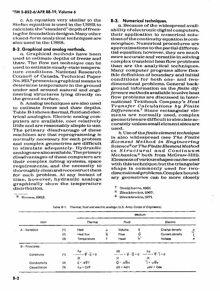
*TM 5-852-6/AFR 88-19, Volume 6

c. An equation very similar to theStefan equation is used in the USSR tocalculate the "standard" depth of freezing for foundation designs. Many otherclosed-form analytical techniques arealso used in the USSR.B-2 . Graphical and analog methods.

a. Graphical methods have beenused to estimate depths of freeze andthaw. The flow net technique can beused to estimate steady-state tempera-ture conditions. National ResearchCouncil of Canada, Technical Paper.No . 163,g presents a graphical means todetermine temperature in the groundunder and around natural and engi-neering structures lying directly onthe ground surface.

b. Analog techniques are also usedto estimate freeze and thaw depths .Table B-1 shows thermal, fluid and electrical analogies. Electric analog com-puters are available, cost relativelylittle and are reasonably simple to use.The primary disadvantage of thesemachines are that reprogramming is;normally necessary for each problemand complex geometries are difficultto simulate adequately . Hydraulicanalogs are also available. The primarydisadvantages of these computers aretheir complex tubing systems, spacerequirements, and the necessity tothoroughly clean and reconstructthem.for each problem. At any instant oftime, however, hydraulic analogsgraphically show the temperaturedistribution .

B-2

Brown, 1663.

B-3.

Numerical techniques.a. Because of the widespread avail-

ability ofelectronic digital computers,their application to numerical solutions ofthe continuity equation is com-monplace . Numerical procedures areapproximations to the partial differen-tial equation; however, they are muchmore accurate and versatile in solvingcomplex transient heat flow problemsthan are the analytical techniques.Many computer programs allow flex-ible definition of boundary and initialconditions for both one- and two-dimensional problems. General back-ground information on the finite dif-ference methods available to solve heatflow problems are discussed in Inter-national Textbook Company's HeatTransfer Calculations by FiniteDifferences. 7 Since rectangular ele-ments are normally used, complexgeometries are difficult to simulate ac-curately unless small element sizes areused.

b. Use ofthefinite elementtechniqueis also widespread (see The FiniteElement Method in EngineeringSciences or TheFiniteElementMethodin Structural and ContinuumMechanics, 9 both from McGraw-Hill) .Elements ofvarious shapes can be usedwith this technique; but the triangularshape is commonly used for two-dimensional problems. Complexbound-ary geometries can be more closely

7 Dusinberre,1961.Zienkiewicz,1967 .

9 Zienkiewicz,1971 .

Table B-1 . Thermal, fluid and electric analogs (U.S. Army .Corps of Engineers) .

Medium

Item Thermal Fluid Electric

A - Variables (1) Heat u Volume S Charge density _p(2) Heat flux 4 Flow Q Current density -'j(3) Temperature T Head H Voltage e

B - Principles :au as ap

Continuity (1) +V-a=o +V . d=o +V .i=oat at at

Conductivity (2) q = -kVT d = -kVH j = -UVeCapacitance (3) du=CdT dS = AdH pdV = Cde

simulated using finite element pro-cedures. For multidimensional heatflow problems, the finite element pro-cedure is frequently more efficient, i.e.,it requires less computer time than thefinite difference technique.

_c. Many flexible computer programs

exist thatsimulate heatconduction andphase change in soils. Each has itsown particular datarequirements,com-

`TM 5-852-6/AFR 88-19, Volume 6

putational capabilities, and acquisitioncosts and restraints. USACRREL hascompleted and documented a modelthat may be useful in solving manyanalytical problems related to construc-tion in the Arctic andSubarctic; othermodels are under development. Con-tact HQ (DAEN-ECE-G) or HQ AFESCfor assistance in selecting an appro-priate model.

APPENDIX C

REFERENCES

Government PublicationsDepartments of theArmy and theAirForce.TM 5-818-2/AFM 88-6, Chapter 4

Pavement Design for Seasonal FrostConditions

TM 5-852-1/AFR 88-19, Volume 1

Arctic andSubarctic Construction,General Provisions

TM 5-852-4/AFM 88-19, Chapter4

Arctic and Subarctic Construction,Building Foundations

TM 5-852-5/AFR 88-19, Volume 5

Arctic and Subarctic Construction,Utilities

'TM 5-352-6/AFR 88-19, Volume 6

Nongovernment PublicationsAmerican Society ofHeating, Refrigeration, andAir-Conditioning Engineers(ASHRAE)345 East 47th Street, New York,N.Y. 10017ASHRAE Guide and Data Book (1963)

Aitken,G.W. andR.L. Berg (1968) Digitalsolution of modified Berggren equa.tion'to calculate depths of freeze andthaw in multilayered systems. Han-over, N.H. : U.S . Army Cold RegionsResearch and Engineering Labora-tory, Special Report 122.

Albert, M.R. (1983) Computer modelsfor two-dimensional transient heatconduction . CRREL Report 83-12.Hanover, N.H. : U.S. Army Cold Re-gions Research and EngineeringLaboratory.

Aldrich, H.P. and H.M. Paynter (1963)Frostinvestigations, fiscal year 1963,first interim report, analytical studiesof freezing and thawing of soils .ACFELTechnicalReport42.Hanover,N.H. : U .S. Army Cold Regions Re-search and Engineering Laboratory.

Alter, A.J . (1969) Water supply in coldregions . CRREL Monograph III-C5a .Hanover, N.H. : U .S. Army Cold Re-gions Research and EngineeringLaboratory.

Alter, A.J . (1969) Sewerage and sewagedisposal disposal in cold regions.CRRELMonograph III-C6b. U.S. ArmyCold Regions Research and Engi-neering Laboratory.

Arctic Construction and Frost EffectsLaboratory (1966) Design and opera-tion ofanhydraulic analogcomputerfor studies of freezing and thawingof soils. ACFELTechnical Report 62.Hanover, N.H.: U.S . Army Cold Re-gions Research and EngineeringLaboratory.

Arctic Constructionand Frost EffectsLaboratory (1968) Frost investiga-tions, 1962-1963. Cold room studies,third interim report ofinvestigations.ACFEL Technical Report 43/1. Han-over, N.H. : U.S. Army Cold RegionsResearch and Engineering Labora-tory.ASHRAE (1963) Air Conditioning Re-frigeration DataBook,DesignVolume.New York: American Society of

BIBLIOGRAPHY

*TM 5-852-6/AFR 88-19, Volume.6

Heating, Refrigerating and Air-Conditioning Engineers .

Barthelemy, J.L. (1980) Performance ofnatural convection heat exchangesystem for subgrade cooling ofperma-frost . CRREL Special Report 80-40.Hanover, N.H. : U.S. Army Cold Re-gions Research and EngineeringLaboratory .

Baumeister, T. (ed.) (1968) MechanicalEngineers Handbook, 6th Ed. NewYork: McGraw-Hill.

Berg, R.L . (1976) Thermoinsulatingmediawithinembankments onperen-nially frozen soil . CRREL SpecialReport 76-3. Hanover,N.H. : U.S. ArmyCold Regions Research and Engi-neering Laboratory.

Brown,W.G . (1963)Graphical determina-tion of temperature under heated orcooled areas on the ground surface.Ottawa: Division ofBuildingResearch,National Research Council ofCanada,Technical Paper No. 163.

Carey, K.L. (1982) The freezing andblockingof water pipes. Cold RegionsTechnical Digest, 82-1. Hanover,N.H.-.U.S. ArmyCold Regions Research andEngineering Laboratory.

Carslaw, H.S . and J.C. Jaeger (1969)Conduction of Heat in Solids, 2ndedition. London: Oxford UniversityPress, Inc.

Corruccini, R.J . and J.J . Gnlewek (1960)Specific heatsand enthalpies of tech-nical solids at low temperatures .National Bureau of Standards Mono-graph 21. Washington, D.C.

Crory, F.E. (1963) Pile foundations inpermafrost. In Permafrost: Pro-ceedings, International Conference,Purdue University. NAS-NRCPublica-tion No. 1287. Washington, D.C., pp.467-472 .

Dusinberre, G.M. (1961) Heat TransferCalculations by Finite Differences.Pennsylvania: International TextBook Company.

Biblio- 1

*TM 5-852-6/AFR 88-19, Volume 6Farouki,O.T. (1981) Thermal propertiesof soils. CRRELMonograph 81-1 . Han-over, N.H.: U.S. Army Cold RegionsResearch and Engineering Labora-tory.

Gilpin, R.R. (1977) The effects of den-dritic ice formation in water pipes .International Journal of Heat andMass Transfer, vol. 20, pp. 693.

Gilpin,RA. (1977) A study ofpipe freez-ingmechanisms. In Utilities Deliveryin Arctic Regions. Ottawa : Environ-mental Protection Service, Environ-"ment Canada, Report No. EPS 3-WP-77-1, pp. 207-220 .

Gilpin, R.R. (1978) A study of factorsaffecting the ice nucleation tempera-ture in a domestic water supply. TheCanadianJournal of ChemicalBngi-neering, vol. 56, pp.466-471 .

Gilpin, R.R. (1979) The morphology ofice structure in a pipe at or neartransition Reynolds numbers. HeatTransfer. San Diego: American In-stitute of Chemical Engineers Sym-posiumSeries 189, vol. 75, pp. 89-94.

Gilpin, R.R. (1981) Ice formation in apipe containing flows in the transitionand turbulent regimes . ASMBJournalofHeat Transfer, vo1.103, pp.363-368.

Ingersoll, L.R., O.J . Zobel and A.C. Inger-soll (1954) HeatConduction: With.Engi-neering, Geological and Other Ap-plications. Madison: University ofWisconsin Press.

Jakob, M. and G.A. Hawkins (1957) Ble-ments of Heat Transfer and Insula-tion, 3rd Ed. New York: John Wileyand Sons, Inc.

Johnson, P .R. (1971) Empirical heattransfer rates ofsmall, Longand Balchthermal piles and thermal convectionloops. Fairbanks: Institute of ArcticEnvironmental Engineering, Univer. .sity of Alaska, Report 7102.

Jennings,B.H. andS .R . Lewis (1968)AirConditioning andRefrlgeration,. 4th.Ed. Pennsylvania: International Text-book Co.

Kaplar, C.W. (1978) Effects of moistureand freeze-thaw on rigid thermal in-sulations :A laboratory investigation.InProceedings of the Conference onApplied TechniquesforColdBnviron-

Biblio-2

ments, Cold Regions Specialty Con-ference, Anchorage, Alaska. NewYork: ASCE.

Kersten, M.S. (1949) Laboratory re-search for the determination of thethermal properties of soils. ACFELTechnical Report 23. Hanover, N.H. :U.S . ArmyCold Regions Research andEngineering Laboratory.

Lachenbruch, A.H. (1957) Three-dimen-sional heat conduction in Permafrostbeneath heated buildings. U.S . Geo-logical Survey Bulletin 1062-B .

Lachenbruch,A.H. (1959) Periodic heatflowin stratified medium with applica-tion topermafrost problems.U.S . Geo-logical Survey Bulletin 1083-A .

Luikov, A.V . (1966)Heat and MassTransferin Capillary-PorousBodies.(Translated from Russian by P.W.B.Harrison.) London: Pergamon Press,Ltd.

Lunardini, V.J . (1981) Heat Transfer inCold Climates . New York: VanNostrand Reinhold Co.

Mallory, S.F. (1969)Thermallnsulation.New York: Van Nostrand ReinholdCo.M.I.T . (1957) Frost penetration in multi-layer soil profiles . ACFELTechnicalReport 67. Hanover, N.H.: U.S. ArmyCold Regions Research and Engi-neering Laboratory.

McAdams (1954) Heat Transmission,3rd Ed. New York: McGraw-Hill .

Porkhaev, G.V. and V .F. Zhukov (1972)Standard depth of freezing of soilsfor foundation engineering purposes.Osnovaniya, Fundamenty i Mek-hanikaGruntov, no.6 (TranslatedfromRussian by Plenum PublishingCorp.,Consultants Bureau). NewYork.

Quinn,W.F. and E.F. Lobacz (1962) Frostpenetration beneath concrete slabsmaintained free ofsnowand ice, withand without insulation. HighwayResearch Board Bulletin 331,pp. 98-115.

Sanger, F.J . (1968) Ground freezing inconstruction . CRREL MiscellaneousPaper 404. Hanover, N.H. : U.S. ArmyCold Regions Research and Engi-neering Laboratory.

Sanger, F.J. and F.H. Sayles (1978)Thermal and rheological computa-

tions for artificially frozen groundconstruction. CRREL MiscellaneousPaper 1216 . Hanover, N.H. : U.S. ArmyCold Regions Research and Engi.neering Laboratory.

Scott, R.F. (1964) Heat exchange at theground surface. CRREL MonographII-A1. Hanover, N.H.: U.S . Army ColdRegions Research and EngineeringLaboratory .

The Engineering Equipment UsersAssociation (1966) Thermal insulationof industrial buildings . EEVAHand-

U.S. GJVEXA4Nf PRINTING OMQ{ 1988,!06-982/80019

'TM 5-852-6/AFR 88-19, Volume 6

book No. 14. London: Constable andCompany, Ltd.

Wilkes, G.B. (1960) HeatInsulationNewYork: John Wiley and Sons, Inc.

Zienkiewicz, O.C. (1967) TheFinite Ele-ment Method in Structural and Con-tinuumMechanics. London: MeGraw.Hill PublishingCo., Ltd.

Zienkiewicz, O.C. (1971) TheFinite Ele-mentMethod inEngineering Science.London: McGraw-Hill PublishingCo.,Ltd.

Biblio-3

R.L. DILWORTHBrigadier General, United StatesArmy

TheAdjutant General

The proponent agency of this publication is the Office of the Chiefof Engineers, United States Army. Users are invited to sendcomments and suggested improvements on DA Form 2028(Recommended Changes to Publications and Blank Forms) direct toHODA(CEEC-EG), WASH, DC 20314-1000.

By Order of the Secretaries of the Army and the Air Force:

CARL E. VUONO'General, United States Army

Official:

ChiefofStaff

LARRYD. WELCH, General, USAFOfficial :

Chief ofStaffWILLIAM O. NATIONS, Colonel, USAFDirector ofInformation ManagementandAdministration

DISTRIBUTION :To be distributed in accordance with DA Form 12-34B, Require-

ments for Arctic and Subarctic Construction .

PIN:

024920 000