Embed Size (px)
Citation preview
3:
G
(C, ,C.
,...3
,
P . I
,,4
.-.,
"5"- ".
..,,-'.
J "l
C -r
_s
# #: _:ii!; : i TMI
:>
¢,,)0I::1
'll;q
https://ntrs.nasa.gov/search.jsp?R=19900020108 2020-01-07T02:47:01+00:00Z
I
l
,tllti||ltll/lllllill/lillili_tuilitiililtlitiili_ii_li_li_i_i_'_ _i_'_ _ _"_'_'_ .......................................................................................................................
NASA Contractor Report 4325
Suspension Systems for Ground
Testing Large Space Structures
Ronald R. Gold, Inger P. Friedman,
and Wilmer H. Reed III
Dynamic Engineering, Inc.
Newport News, Virginia
W. L. Hallauer
Virginia Polytechnic Institute and State University
Aerospace and Ocean Engineering Department
Blacksburg, Virginia
Prepared for
Langley Research Center
under Contract NAS1-18798
National Aeronautics andSpace Administration
Office of Management
Scientific and TechnicalInformation Division
1990

TABLE OF CONTENTS
TABLE OF CONTENTS ............................. ii±
LIST OF FIGURES ................................. vi
SUMMARY ..................................... ix
1.0 INTRODUCTION ................................... 1
2.0 TEST APPARATUS ................................. 3
3.0 VERTICAL SUSPENSION SYSTEM ...................... 4
3.1 Description ................................... 4
3.2 Analytical Development ........................... 5
3.3 Experimental Test Set-Up ......................... 8
3.4 Performance Characteristics/Test Results ............. 10
4.0 LATERAL SUSPENSION ............................ 13
4.1 Moving Cart Analogy ........................... 14
4.2 Damping Effects ............................... 15
5.0 TORSION SUSPENSION ............................ 18
5.1 Description of Concept .......................... 18
5.2 Test Results .................................. 19
5.3 Application to Evolutionary Model .................. 20
iii
-" ,, ....... r mL iyd I_.,i.,J
TABLE OF CONTENTS, CON'T
6.0 PASSIVE LATERAL/TORSION ANALYTICAL MODEL ........ 22
6.1 Equations of Motion ............................ 22
6.2 Undamped Vibration Modes ...................... 27
6.2.1 Cart Fixed (2-DOF Model) .................... 27
6.2.2 Cart Free (3-DOF Model) .................... 28
6.3 Damped Vibration Modes ........................ 28
7.0 ACTIVE CONTROL OF LATERAIJTORSlON SUSPENSION .... 30
7.1 General Design Considerations .................... 30
7.2 Proportional Control ............................ 33
7.3 Proportional-Integral-Derivative Control ............... 35
7.4 Experimental Results ........................... 38
8.0 CONCLUDING REMARKS ........................... 40
9.0 REFERENCES ................. .................. 42
APPENDIX A, SUSPENSION SYSTEM ASSEMBLY PROCEDURE 43
APPENDIX B, PC-MATLAB DATA FILES ................. 48
B.1, 2-DOF Model of Full System in 1-g with Cart Fixed ..... 48
B.2, 2-DOF Model of Test Structure in 0-g .............. 52
B.3, 3-DOF Model of Undamped Full System in 1-g ........ 54
iv
TABLE OF CONTENTS, CON'T
B.4, Damping Constant Representing Linear Bearing Friction 57
B.5, Proportional Control ........................... 58
B.6, Rigid Body Modes ............................ 60
B.7, PID Control ................................. 62
APPENDIX C, DIGITAL CONTROLLER PROGRAM .......... 64
v
LIST OF FIGURES
Figure 1.
Figure 2.
Figure 3.
Figure 4.
Figure 5.
Figure 6.
Figure 7.
Figure 8a. Vertical Suspension Test Results, 145 Ib Load
Figure 8b. Vertical Suspension Test Results, 80 Ib Load
Figure 8c.
Figure 9a.
Vertical Suspension Test Apparatus .................. 68
Lateral/Torsion Suspension Test Apparatus ............. 69
Zero Spring Rate Mechanism (ZSRM) ................ 70
ZSRM Stiffness Characteristics ...................... 71
Effect of Side Spring Preload on System Frequency ...... 72
3-DOF Suspension Test Apparatus .................. 73
Stiffness and Frequency Comparisons,
Main Spring vs. ZSRM ............................ 74
.......... 75
........... 76
Vertical Suspension Test Results, 42.5 Ib Load .......... 77
Comparison of Analytical and Experimental Results,145 Ib Load
................................... 78
Figure 9b. Comparison of Analytical and Experimental Results,80 Ib Load
..................................... 9
Figure 10. Change in Frequency with Side Spring Vertical Location ... 80
Figure 11. Change in _ with Frequency ....................... 81
Figure 12. Moving Cart Analogy ............................. 82
Figure 13. Lateral Suspension Model ......................... 83
Figure 14. Effect of Cart Damping on Lateral-Mode Root ........... 84
vi
LIST OF FIGURES, CONT'D
Figure 15. Equivalent Viscous Damping of Carton Linear Bearing ............................... 85
Figure 16. Linear-Bearing Breakout Force Coefficient ............. 86
Figure 17. Low-Frequency Torsional Suspension System ........... 87
Figure 18. Effect of h on Frequency Spectra of TorsionSuspension System ............................. 88
Figure 19. Phase Zero Evolutionary Model with Torsion Suspension . .. 89
Figure 20. Phase Zero Evolutionary Model with Torsion Suspension -1st Torsion Mode ............................... 90
Figure 21. Test Article Geometry and DOFs .................... 91
Figure 22. Natural Frequencies of the Lateral/Torsion Systemwith Cart Fixed ................................. 92
Figure 23. Natural Frequencies of the Lateral/Torsional Systemwith Cart Free .................................. 93
Figure 24. Transient Response of Damped 1-g 3-DOF Model,
Xc(t ) is solid, xo(t) is dot dash ....................... 94
Figure 25. Effect of Active Control on Lateral-Mode Root
Control Force Fc = Cp(X2-X 1) ....................... 97
Figure 26. Zero Stiffness Open-Loop Loci of Roots as c,, Varies
from 0 thru 0.4 (mg = 100 Ib, m,,g = 5.65 Ib,
h = 17.5 in, L = 62.12 in) ......................... 98
Figure 27. Zero-Stiffness Proportional-Control Loci ofRoots d/b = 1 ................................. 99
vii

LIST OF FIGURES, CONT'D
Figure 28. Loci of Roots for P, PD, and PI Types of Control for
h = 0", d/b = 1.084, c,, = 0.5 Ib/ips, -r = 0.025 sec ...... 101
viii
SUMMARY
This report documents a research program for the development of improved suspension
techniques for ground vibration testing of large, flexible space structures. The
suspension system must support the weight of the structure and simultaneously allow
simulation of unconstrained rigid-body movement as in the space environment.
Exploratory analytical and experimental studies were conducted for suspension systems
designed to provide minimum vertical, horizontal, and rotational degrees of freedom.
The effects of active feedback control added to the passive system were also
investigated.
An experimental suspension apparatus was designed, fabricated and tested. This test
apparatus included a zero spring rate mechanism (ZSRM) designed to support a range
of weights from 50 to 300 Ibs and provide vertical suspension mode frequencies less
than 0.1 Hertz (Hz).
The lateral suspension consisted of a pendulum suspended from a moving cart (linear
bearing) which served to increase the effective length of the pendulum. The torsion
suspension concept involved dual pendulum cables attached from above to a pivoting
support (bicycle wheel). A simple test structure having variable weight and stiffness
characteristics was used to simulate the vibration characteristics of a large space
structure.
The suspension hardware for the individual degrees of freedom was analyzed and tested
separately and then combined to achieve a 3 Degree-of-Freedom (DOF) suspension
system. Results from the exploratory studies should provide useful guidelines for the
ix

development of future suspension systems for ground vibration testing of large space
structures.
This research program was conducted under NASA Langley Research Center Contract
NAS1-18798 funded by the Controls-Stuctures Interaction Guest Investigator Program.
1.0 INTRODUCTION
The proposed use of large space structures has created unique and challenging
requirements. The extremely large size and light weight of the structures coupled with
the near zero gravity, vacuum environment of space causes difficulty with the control and
movement of such structures. To understand and document these difficulties a
significant number of ground-based tests on sample or model large space structures will
be required. Ground Vibration Tests (GV'F's) are necessary to characterize a structure's
behavior under dynamic conditions such as slewing a large space antenna or performing
a docking maneuver with a space station. Ground Vibration Tests provide the engineer
with data specifying the structure's natural modes, frequencies, damping, and mode
shapes. These data are critical in determining methods of moving and controlling large,
lightweight space structures.
One of the major difficulties with ground vibration testing of large space structures is
suspending the structure to allow freedom of motion similar to that found in space. It is,
of course, impossible to match the near zero gravity environment of space in ground-
based facilities, therefore, suspension systems must support the structure and must do
so in a manner that does not overly constrain its motion. The structural members
themselves are not designed to take significant loads such as the weight loading which
occurs in a ground test environment. Therefore, the suspension system must, while
allowing freedom of motion, adequately distribute the weight loading throughout the frail
structural members. Freedom of motion requires that the suspension system allow the
structure rigid-body movement, that is, minimal coupling with the flexible or vibrational
modes of the structure. This freedom is required to adequately simulate movement of
the structure in space.
The extremely large size and relative frailty of the structures themselves, or even scaled
models of the structures, create unique problems associated with suspension systems.
These large structures typically have extremely low natural frequencies. The fundamental
frequencies will often be below 0.5 Hz. The addition of a suspension system creates
non-zero rigid body modes of the large space structure. The frequency of the rigid
body modes is dependent on the suspension stiffness. To adequately uncouple the
rigid body modes of the structure from the fundamental flexible modes, the rigid body
modes should have frequencies substantially lower than the first fundamental mode.
Attempts are often made to suspend structures with long cables, pendulum fashion, from
a high ceiling. However, at the extremely low frequencies involved, the required cable
lengths become prohibitively long.
Pendulum cable supports limit structural testing to one plane of motion at a time. This
support technique ignores the coupling of structural modes in more than one plane and
does not address the distortion of torsion modes of beam-like structures nor the
distortion of bending modes in the vertical plane. Improved suspension systems using
both active and passive technologies have been proposed for support of large space
structures. It is felt that initial improvements using simple passive techniques should be
examined as a starting point and supplementedwith active systems as necessary. As
such, this report will document studies, both passive and active, which provide improved
suspension in three degrees-of-freedom. Techniques will be described which "effectively"
lengthen fixed pendulum cables and which offer soft suspension in both the vertical and
torsional degrees of freedom.
2
2.0 TEST APPARATUS
An illustration of the apparatus used to provide a soft vertical suspension is shown in
Figure 1. The main springs bear the weight of the large space structure (represented
by laboratory weights in the figure), but the dynamic stiffness of the system is decreased
by the addition of the side spring forces. The system tested was designed to support
a range of payloads from 50 to 300 Ibs and to provide a minimum suspended frequency
of less than 0.1 Hz. The suspension system is designed to allow a vertical travel of _+
3 inches. A complete description of the mechanism and its performance is included in
Section 3.0 of this report.
The coupled lateral/torsion suspension system is shown conceptually in Figure 2. The
soft lateral suspension is provided by a linear bearing which serves to effectively
lengthen the support cables. The torsion suspension is shown as a simple wheel
concept. In the laboratory tests a good quality bicycle wheel was used for the torsion
suspension because it best met the overall requirements of minimum weight, high load
capacity, minimum bearing friction, and low cost. The choice of a bicycle wheel is not
surprising since the basic design of such wheels has been optimized over many years.
For more heavy duty (high payload) requirements a simple three-bar linkage may be
substituted. Complete descriptions of the lateral and torsion suspension devices are
included in Sections 4.0 and 5.0, respectively.
While originally analyzed and tested independently, the vertical suspension and the
lateral/torsion suspension were coupled as a three degree-of-freedom (DOF) suspension
in later tests. The lateral and torsion suspension are heavily coupled and have been
analyzed and tested together. Coupling the vertical suspension to the lateral/torsion was
3
not significant in that they are basically uncoupled. However, the addition of the vertical
suspension did complicate the active control system as described in Section 7.0.
In order to test the suspension systems, a simple test structure was fabricated which
simulated the characteristics of a large space structure. Also shown in Figure 2, the
simulated structure is a rigid frame loaded with laboratory weights and restrained
elastically by three long rods. The structure is designed to have three basic low
frequency modes of interest, horizontal (lateral) and vertical translation and rotation
(torsion) in the plane normal to the rods. The lateral and vertical mode natural
frequencies are between 0.2 and 0.3 Hz, and the torsion mode frequency is designed
to be between 1.0 and 2.0 Hz. The structural weight can be varied from 20 to 200 Ibs.
This range of payload and low natural frequencies provide an excellent test bed and
allow a rigorous evaluation of the suspension devices.
3.0 VERTICAL SUSPENSION SYSTEM
3.1 Description
The primary objective of a vertical suspension system is to provide a near zero vertical
stiffness and yet be strong and stiff enough to support a heavy load with a limited
amount of initial deflection. The Dynamic Engineering Incorporated (DEI) vertical
suspension system is based on the concept of a Zero Spring Rate Mechanism (ZSRM)
which has been discussed by others including Kienholz et al in Reference 1. This type
of system can be designed to have very low vertical stiffness characteristics and at the
same time support large loads with moderate initial deflections. The components of the
ZSRM configuration incorporated into the DEI vertical suspension system are shown in
Figure 3a. The weight of the structure is supported by the main vertical spring, which
4
has a spring constant Km. in order to limit the initial deflection of the spring under load,
a relatively stiff spring is used. The ZSRM configuration consists of four linkages, two
vertical and two horizontal. The horizontal members are joined together at one end and
are connected to the vertical members on the opposite ends. The vertical members are
supported at the upper end by a fixed support through a hinge joint. All the
connections between the members are also hinge joints. A horizontal spring, with
stiffness K s stretches between the outward ends of the horizontal members, applying a
compressive force to them.
When the system is in equilibrium, the horizontal members are exactly horizontal and the
vertical members are perpendicular to them. The structural weight is balanced by the
restoring force of the main spring, and the compressive force has no component in the
vertical direction. As the system is deflected away from the neutral point, the
compressive load in the horizontal members develops a vertical component. This vertical
force acts in a direction opposite to the restoring force of the main spring, effectively
reducing the stiffness of the main spring. With the proper combination of springs and
compressive load, the system will exhibit near zero stiffness and will require very little
force to deflect it from the neutral point. The structural weight will behave as if it is
floating.
3.2 Analytical Development
The vertical suspension system was analyzed to determine the best configuration by
examining the effect of each of the design parameters on the behavior of the system.
By summing the vertical forces acting at the center point (see Figure 3b), the restoring
force, F R, can be determined from the following equation:
5
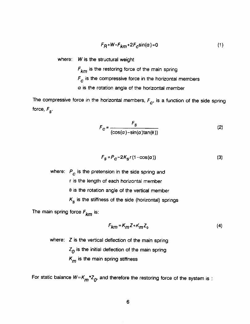
FR + W-Fkm +2Fcsin(o ) =0 (I)
where: W is the structural weight
Fkm is the restoring force of the main spring
F c is the compressive force in the horizontal members
a is the rotation angle of the horizontal member
The compressive force in the horizontal members, Fc, is a function of the side spring
force, F s.
FsF c = (2)
(cos(a)-sin(a)tan(O))
F s = Pc-2K s r (1 -cos(a )) (3)
where: Pc is the pretension in the side spring and
r is the length of each horizontal member
e is the rotation angle of the vertical member
Ks is the stiffness of the side (horizontal) springs
The main spring force Fkm is:
Fkm =KmZ*KmZ o
where: Z is the vertical deflection of the main spring
Z 0 is the initial deflection of the main spring
K m is the main spring stiffness
(4)
For static balance W=Km*Zo, and therefore the restoring force of the system is :
6
2Fssin(a)F R = K m Z - (5)
cos(a) - sin(a) tan({) )
For small values of Z, angle e is very small and the equation for F R can be reduced to
the following:
F R = KmZ - 2F s tan(a) (6)
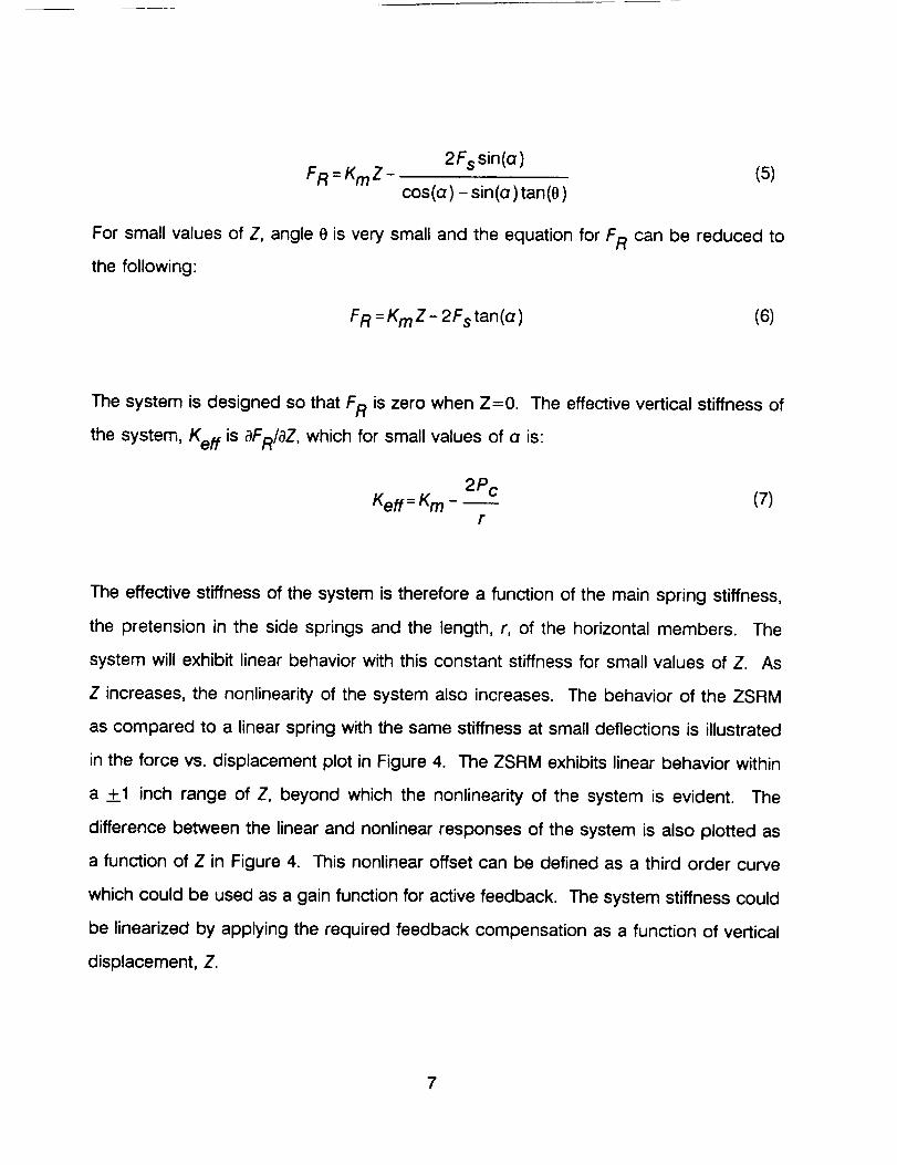
The system is designed so that FR is zero when Z=0. The effective vertical stiffness of
the system, Keff is aFR/aZ, which for small values of a is:
2P cKeff= Km - _ (7)
r
The effective stiffness of the system is therefore a function of the main spring stiffness,
the pretension in the side springs and the length, r, of the horizontal members. The
system will exhibit linear behavior with this constant stiffness for small values of Z. As
Z increases, the nonlinearity of the system also increases. The behavior of the ZSRM
as compared to a linear spring with the same stiffness at small deflections is illustrated
in the force vs. displacement plot in Figure 4. The ZSRM exhibits linear behavior within
a +1 inch range of Z, beyond which the nonlinearity of the system is evident. The
difference between the linear and nonlinear responses of the system is also plotted as
a function of Z in Figure 4. This nonlinear offset can be defined as a third order curve
which could be used as a gain function for active feedback. The system stiffness could
be linearized by applying the required feedback compensation as a function of vertical
displacement, Z.
7
The nonlinearity of the system is a function of several parameters, including Km, Ks, r
and L, where L is the length of the vertical members. In general, for a given structural
weight, decreasing the stiffness of the springs (while maintaining the correct Km/K s ratio)
will reduce the nonlinearity of the system. However, a reduction in Km is limited by
strength requirements and limits on the static deflection of the spring. The stiffness of
the system is not symmetric with respect to the Z direction, due to the motion of the
vertical member. As L increases, e decreases to the point where there is no motion of
the vertical members within the vertical travel limit of the system. If e is zero the stiffness
will be symmetric with respect to the Z direction. Physical limitations on the length of the
vertical members must be considered, however, when designing the system.
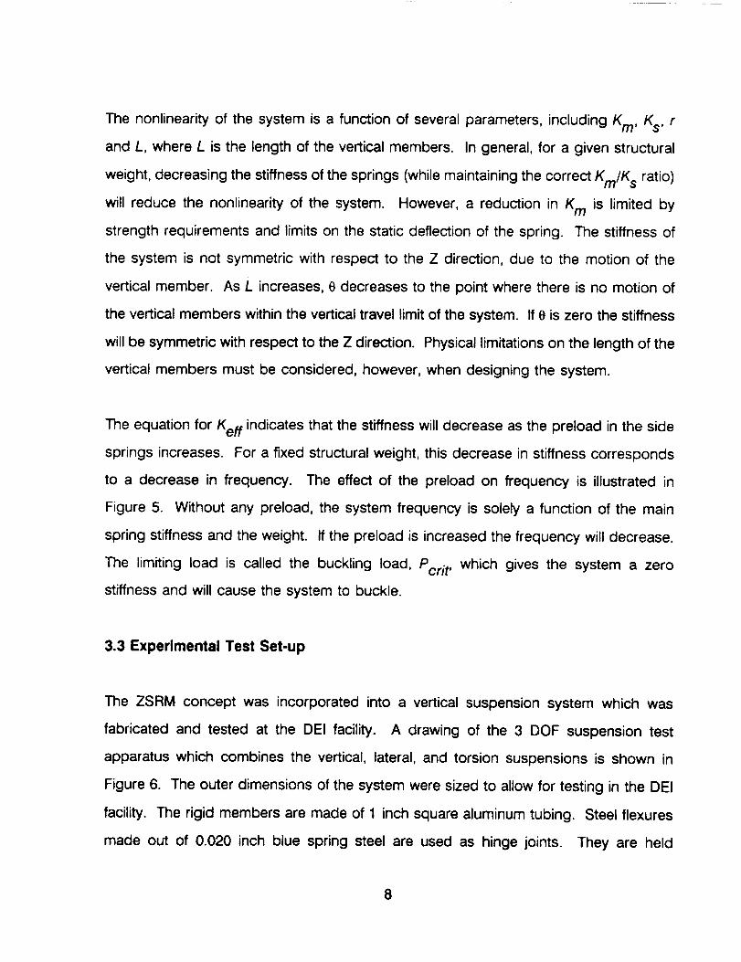
The equation for Keff indicates that the stiffness will decrease as the preload in the side
springs increases. For a fixed structural weight, this decrease in stiffness corresponds
to a decrease in frequency. The effect of the preload on frequency is illustrated in
Figure 5. Without any preload, the system frequency is solely a function of the main
spring stiffness and the weight. If the preload is increased the frequency will decrease.
The limiting load is called the buckling load, Pcrit' which gives the system a zero
stiffness and will cause the system to buckle.
3.3 Experimental Test Set-up
The ZSRM concept was incorporated into a vertical suspension system which was
fabricated and tested at the DEI facility. A drawing of the 3 DOF suspension test
apparatus which combines the vertical, lateral, and torsion suspensions is shown in
Figure 6. The outer dimensions of the system were sized to allow for testing in the DEI
facility. The rigid members are made of 1 inch square aluminum tubing. Steel flexures
made out of 0.020 inch blue spring steel are used as hinge joints. They are held
8
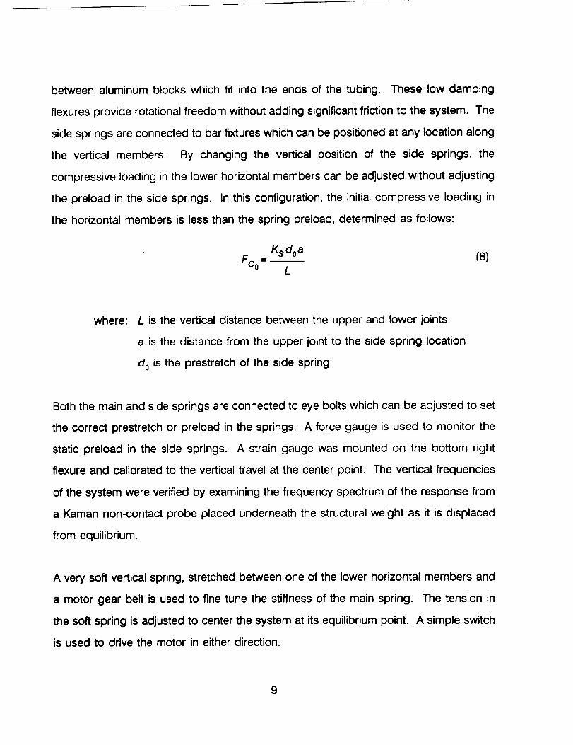
between aluminum blocks which fit into the ends of the tubing. These low damping
flexures provide rotational freedom without adding significant friction to the system. The
side springs are connected to bar fixtures which can be positioned at any location along
the vertical members. By changing the vertical position of the side springs, the
compressive loading in the lower horizontal members can be adjusted without adjusting
the preload in the side springs. In this configuration, the initial compressive loading in
the horizontal members is less than the spring preload, determined as follows:
K s d oa (8)Fc° - L
where: L is the vertical distance between the upper and lower joints
a is the distance from the upper joint to the side spring location
d o is the prestretch of the side spring
Both the main and side springs are connected to eye bolts which can be adjusted to set
the correct prestretch or preload in the springs. A force gauge is used to monitor the
static preload in the side springs. A strain gauge was mounted on the bottom right
flexure and calibrated to the vertical travel at the center point. The vertical frequencies
of the system were verified by examining the frequency spectrum of the response from
a Kaman non-contact probe placed underneath the structural weight as it is displaced
from equilibrium.
A very soft vertical spring, stretched between one of the lower horizontal members and
a motor gear belt is used to fine tune the stiffness of the main spring.
the soft spring is adjusted to center the system at its equilibrium point.
is used to drive the motor in either direction.
The tension in
A simple switch
9
This experimental vertical suspension was designed to support a maximum load of 300
Ibs. The range of vertical travel is +3 inches. Protective stops have been installed on
the system to prevent any further travel which could damage the flexures. Two different
spring combinations were tested on this system, the first with a load capacity of 150 Ibs
and the second with a load capacity of 50 Ibs. Complete instructions for the assembly,
installation and tuning of the vertical system are included in Appendix A.
This type of vertical suspension system can be customized to a large range of weight
Ioadings by installing the appropriate combination of main and side springs. The weight
range for a particular spring combination is dependent on the adjustment features
available for large changes in initial deflection of the main spring. The vertical stroke is
limited primarily by flexure deflection limits. The stroke can be increased by lengthening
the horizontal members, which will increase the ratio between the vertical travel and the
deflection of the flexures.
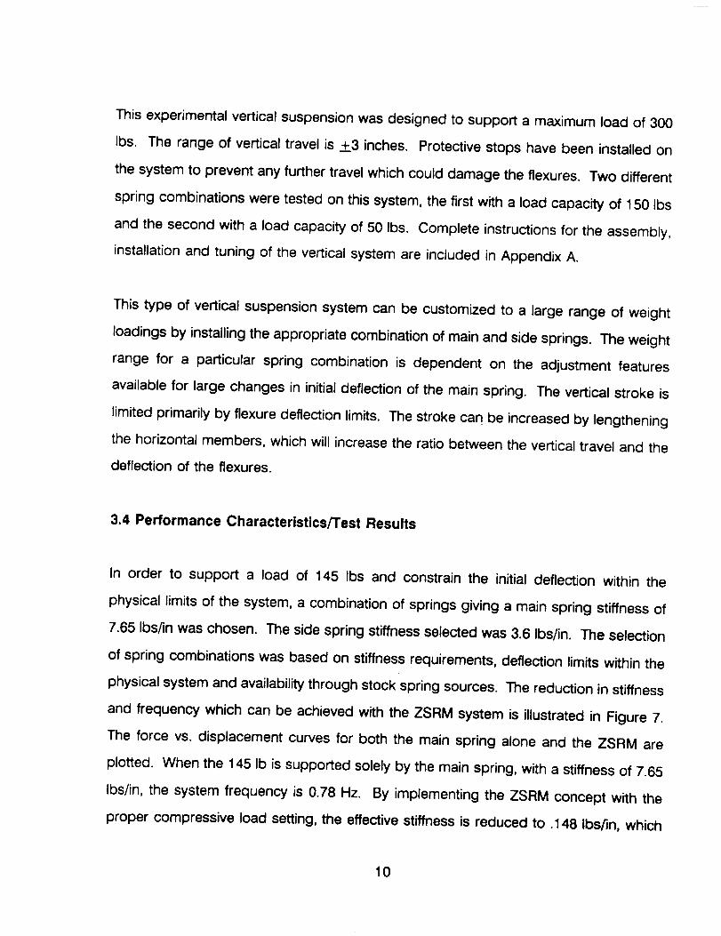
3.4 Performance Characteristics/Test Results
In order to support a load of 145 Ibs and constrain the initial deflection within the
physical limits of the system, a combination of springs giving a main spring stiffness of
7.65 Ibs/in was chosen. The side spring stiffness selected was 3.6 Ibs/in. The selection
of spring combinations was based on stiffness requirements, deflection limits within the
physical system and availability through stock spring sources. The reduction in stiffness
and frequency which can be achieved with the ZSRM system is illustrated in Figure 7.
The force vs. displacement curves for both the main spring alone and the ZSRM are
plotted. When the 145 Ib is supported solely by the main spring, with a stiffness of 7.65
Ibs/in, the system frequency is 0.78 Hz. By implementing the ZSRM concept with the
proper compressive load setting, the effective stiffness is reduced to .148 Ibs/in, which
10
corresponds to a frequency of 0.1 Hz. As mentioned previously, the stiffness of the
ZSRM becomes nonlinear as Z increases. This nonlinearity can be observed in the force
vs. displacement curve for magnitudes of Z greater than one inch.
For a constant supported weight, the frequency of the vertical system can be adjusted
to any value less than the frequency of the main spring by applying the correct
compressive loading to the lower horizontal members. For a given mass, M, and a
desired frequency, _, the required effective stiffness of the system, Keff, is _2*M. The
equation for Keff, derived in the analysis section, can be used to solve for the preload
in the side springs as follows:
pc = (K m _Keff ) rL (9)2a
The force gauge is used to set the correct preload determined from this equation. The
spring deflection is changed by adjusting the location of the eye bolts or the spring
attachment bar. Fine tuning adjustments may be necessary to match the desired
frequency.
Initial attempts at matching frequencies indicated that the vertical stiffness of the system
was higher than expected due to the stiffness of the flexures. In calculating the proper
preload, K m must include the main spring and flexure stiffnesses.
The desired frequency chosen for the experimental test apparatus was 0.1 Hz. The
frequency of the system was verified using a Kaman non-contact probe, placed
underneath the supported weight. The system was displaced from its neutral point
about two inches and allowed to oscillate freely. The frequency spectrum from the
11
probe response was used to determine the frequency. A free response time history and
corresponding frequency spectrum for the vertical system supporting a 145 Ib load are
presented in Figure 8a. The frequency of the vertical mode is 0.105 Hz. The vertical
system was tested with various weight Ioadings to verify that the desired frequencies
could be achieved for a range of weights. The minimum weight tested on the 145 Ib
spring system was 80 Ibs. The 0.1 Hz frequency of this configuration was verified by
the frequency spectrum of the free response, shown in Figure 8b. A second set of
springs was installed for a maximum load of 50 Ibs. The frequency spectrum from the
free response of this configuration with a 42 Ib load is shown in Figure 8c.
Force deflection tests were performed on the various configurations to determine the
restoring force of the system in the +3 inch vertical range. Weight was added to the
system in small increments and deflection measurements were taken for each
incremental weight. The force vs. deflection curve obtained from these measurements
along with the analytical curve are presented in Figure 9a for the 145 Ib case. The
experimental curve demonstrates slightly more nonlinearity for values of Z beyond two
inches, but the differences are relatively small. The force vs. displacement curve shown
in Figure 9b for the vertical system with an 80 Ib load demonstrates similar behavior.
As mentioned previously, the vertical location of the side spring mounting brackets can
be adjusted to provide a means of changing the compressive load in the lower
horizontal members without changing the preload in the side springs. The sensitivity of
this adjustment with respect to compressive loading and frequency is illustrated in Figure
10. The frequency can be reduced from .185 Hz to .068 Hz by lowering the position of
the springs 1.75 inches which corresponds to a 2 Ib change in compressive loading.
This high degree of sensitivity not only allows the system to be tuned for very low
12
frequencies (near zero), but also makes the system more sensitive to changes in
temperature and air disturbances.
Damping measurements were obtained from the free decay response of the system to
an initial deflection. The percent critical damping, _, was calculated using the logarithmic
decrement method. Damping was examined for a range of system frequency settings
corresponding to various levels of compressive loading. The damping measurements
taken from the experimental data are presented in Figure 11. As expected, Z;increases
as frequency decreases. Since there are no moving parts in the system, the source of
the damping must be structural damping in the flexures. At such low frequencies, air
damping could also be a contributing factor.
4.0 LATERAL SUSPENSION
The suspension of large space structures from long pendulum cables provides a
convenient means for allowing the test article to move laterally as a rigid body. To
minimize dynamic coupling of the pendulum and elastic modes of the suspended
structure, excessively long pendulum cables may be required. For the test article
suspended as a simple pendulum with cables fixed at the upper ends, the lowest
suspension mode frequency is
p = Vl-g/ L , rad/sec (10)
where: g is the gravitational constant and
L the support cable length
13
The techniques described below provide a means for increasing the effective length of
pendulum cables. Some of these ideas were originally introduced in Reference 2.
4.1 Moving Cart Analogy
The moving-cart analogy depicted in Figure 12 provides a useful means of studying the
application of extended pendulum techniques such as the inverted pendulum, tensioned-
cable suspension and other techniques for reducing the natural frequency of a simple
pendulum. The primary goal of all of these methods is to reduce the system's
fundamental frequency. This frequency is dependent upon the stiffness of a spring
between the cart and ground. If the spring is infinitely stiff, the suspension system
frequency is g_, the simple pendulum frequency. As the spring stiffness, Kx,
approaches zero, the suspension frequency, (_p, likewise approaches zero.
The tensioned cable may also be replaced with a fixed rail or beam on which a pulley
rides. This system has the advantage that large tensions and long lengths are not
required to lower the restoring force. The restoring spring Kx is controlled by the shape
of the rail, specifically, the depth, d, of the rail. The value of Kx shown in Figure 12 is
for a circular arc shape and yields a linear spring for small motions on the rail. This
system offers very low values of K.x, in fact, the rail can be flat (d = 0), allowing the
restoring force to approach zero.
The system also has a higher-frequency cart mode. For K,
mode frequency, oc, to the simple pendulum frequency is
= 0 the ratio of the cart-
14
w(11)
where W and w are the weights of the suspended structure and the cart respectively.
It is interesting to note that in all cases, the effective spring stiffness Kx, and conse-
quently the suspension system frequency, is strongly dependent on the suspended
weight. This feature differs from the simple pendulum whose frequency is independent
of pendulum weight.
4.2 Damping Effects
In the preceding discussion of lateral suspension systems, the effects of damping or
friction forces were neglected. The effect of such forces acting on the moving cart is
considered next. For ease of analysis, it is assumed throughout that the damping
mechanism can be modeled as an equivalent linear viscous damper. To investigate
damping effects, the lateral suspension model shown in Figure 13 is analyzed. The
definition of parameters and the specific example cases to be considered are also given
in Figure 13. Note that the suspended mass is connected to the ground by a spring
of stiffness k. Thus, _-_M represents the undamped lateral mode frequency of the
"test article" in a zero-gravity (O-g) environment. The equations of motion for the model
shown in Figure 13 are as follows:
15
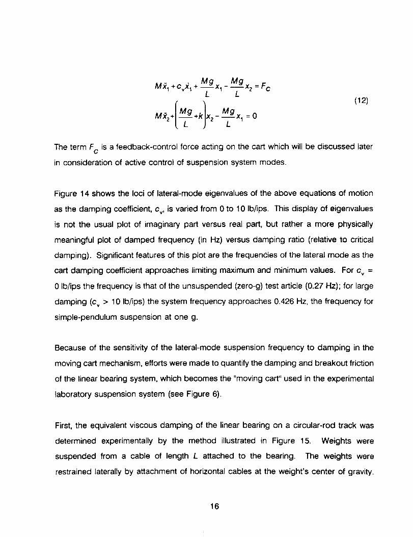
Mn MnM,_ 1 + c,,,_ 1+ '-=xl_ ""_, xz = F c
L L(12)
The term Fc is a feedback-control force acting on the cart which will be discussed later
in consideration of active control of suspension system modes.
Figure 14 shows the loci of lateral-mode eigenvalues of the above equations of motion
as the damping coefficient, c,,, is varied from 0 to 10 Ib/ips. This display of eigenvalues
is not the usual plot of imaginary part versus real part, but rather a more physically
meaningful plot of damped frequency (in Hz) versus damping ratio (relative to critical
damping). Significant features of this plot are the frequencies of the lateral mode as the
cart damping coefficient approaches limiting maximum and minimum values. For c v =
0 Ib/ips the frequency is that of the unsuspended (zero-g) test article (0.27 Hz); for large
damping (c v > 10 Ib/ips) the system frequency approaches 0.426 Hz, the frequency for
simple-pendulum suspension at one g.
Because of the sensitivity of the lateral-mode suspension frequency to damping in the
moving cart mechanism, efforts were made to quantify the damping and breakout friction
of the linear bearing system, which becomes the "moving cart" used in the experimental
laboratory suspension system (see Figure 6).
First, the equivalent viscous damping of the linear bearing on a circular-rod track was
determined experimentally by the method illustrated in Figure 15. Weights were
suspended from a cable of length L attached to the bearing. The weights were
restrained laterally by attachment of horizontal cables at the weight's center of gravity.
16
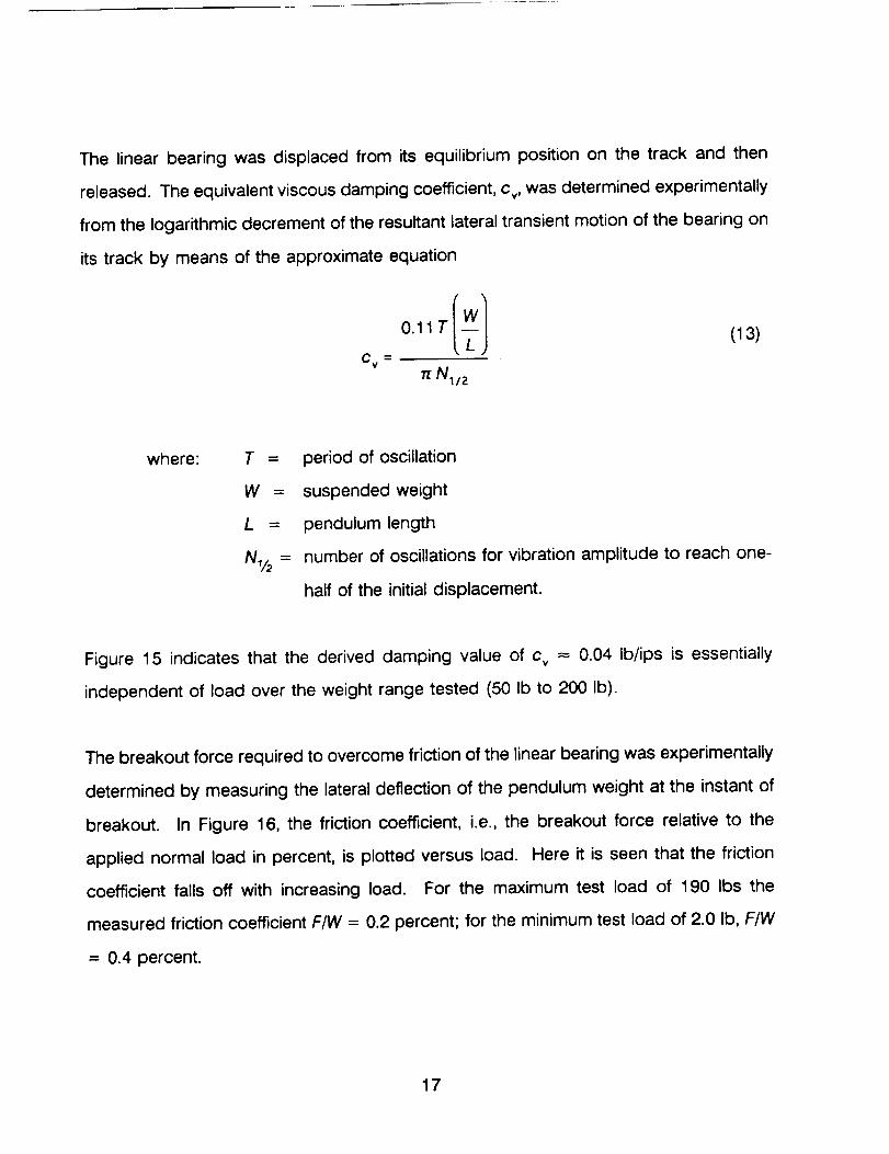
The linear bearing was displaced from its equilibrium position on the track and then
released. The equivalent viscous damping coefficient, c v, was determined experimentally
from the logarithmic decrement of the resultant lateral transient motion of the bearing on
its track by means of the approximate equation
C v
(13)
where: T
W =
L =
N½=
period of oscillation
suspended weight
pendulum length
number of oscillations for vibration amplitude to reach one-
half of the initial displacement.
Figure 15 indicates that the derived damping value of c v = 0.04 Ib/ips is essentially
independent of load over the weight range tested (50 Ib to 200 Ib).
The breakout force required to overcome friction of the linear bearing was experimentally
determined by measuring the lateral deflection of the pendulum weight at the instant of
breakout. In Figure 16, the friction coefficient, i.e., the breakout force relative to the
applied normal load in percent, is plotted versus load. Here it is seen that the friction
coefficient falls off with increasing load. For the maximum test load of 190 Ibs the
measured friction coefficient F/W = 0.2 percent; for the minimum test load of 2.0 Ib, F/W
= 0.4 percent.
17
5.0 TORSION SUSPENSION
In previous sections of the paper, various means of achieving low-frequency suspension
modes in the vertical and lateral directions have been considered. To alleviate coupling
between the suspension system and the structure's torsion modes, there is equal need
for consideration of low-frequency suspension to allow undistorted torsional vibration
modes.
5.1 Description of Concept
Figure 17 shows the proposed low-frequency torsional suspension system. This system
uses a dual cable approach and a rotating support pivot to lower the frequency of the
suspension system's torsion or rotation mode. The body is suspended by two cables
of equal length L from a pivoting support structure. The cables are configured as a
parallelogram such that at rest, the center of gravity of the body hangs directly below
the pivot axis.
The system has two uncoupled natural pendulum modes.
mode whose frequency is described by:
One is the "simple" pendulum
o s = g_, rad/sec (14)
where: g is the gravitational constant
L is the pendulum cable length
18
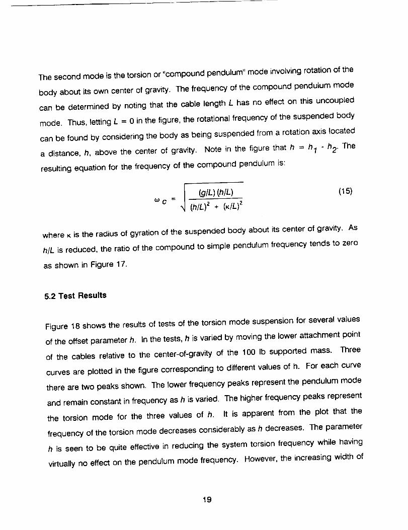
The second mode is the torsion or "compound pendulum" mode involving rotation of the
body about its own center of gravity. The frequency of the compound pendulum mode
can be determined by noting that the cable length L has no effect on this uncoupled
mode. Thus, letting L -- 0 in the figure, the rotational frequency of the suspended body
can be found by considering the body as being suspended from a rotation axis located
a distance, h, above the center of gravity. Note in the figure that h = h 1 - h 2. The
resulting equation for the frequency of the compound pendulum is:
_C = I (g/L) (h/L)(h/L) z + (K/L) z
(15)
where x is the radius of gyration of the suspended body about its center of gravity. As
h/L is reduced, the ratio of the compound to simple pendulum frequency tends to zero
as shown in Figure 17.
5.2 Test Results
Figure 18 shows the results of tests of the torsion mode suspension for several values
of the offset parameter h. In the tests, h is varied by moving the lower attachment point
of the cables relative to the center-of-gravity of the 100 Ib supported mass. Three
curves are plotted in the figure corresponding to different values of h. For each curve
there are two peaks shown. The lower frequency peaks represent the pendulum mode
and remain constant in frequency as h is varied. The higher frequency peaks represent
the torsion mode for the three values of h. It is apparent from the plot that the
frequency of the torsion mode decreases considerably as h decreases. The parameter
h is seen to be quite effective in reducing the system torsion frequency while having
virtually no effect on the pendulum mode frequency. However, the increasing width of
19
the pendulum mode peaks for decreasing values of h indicates an increase in damping
of this mode.
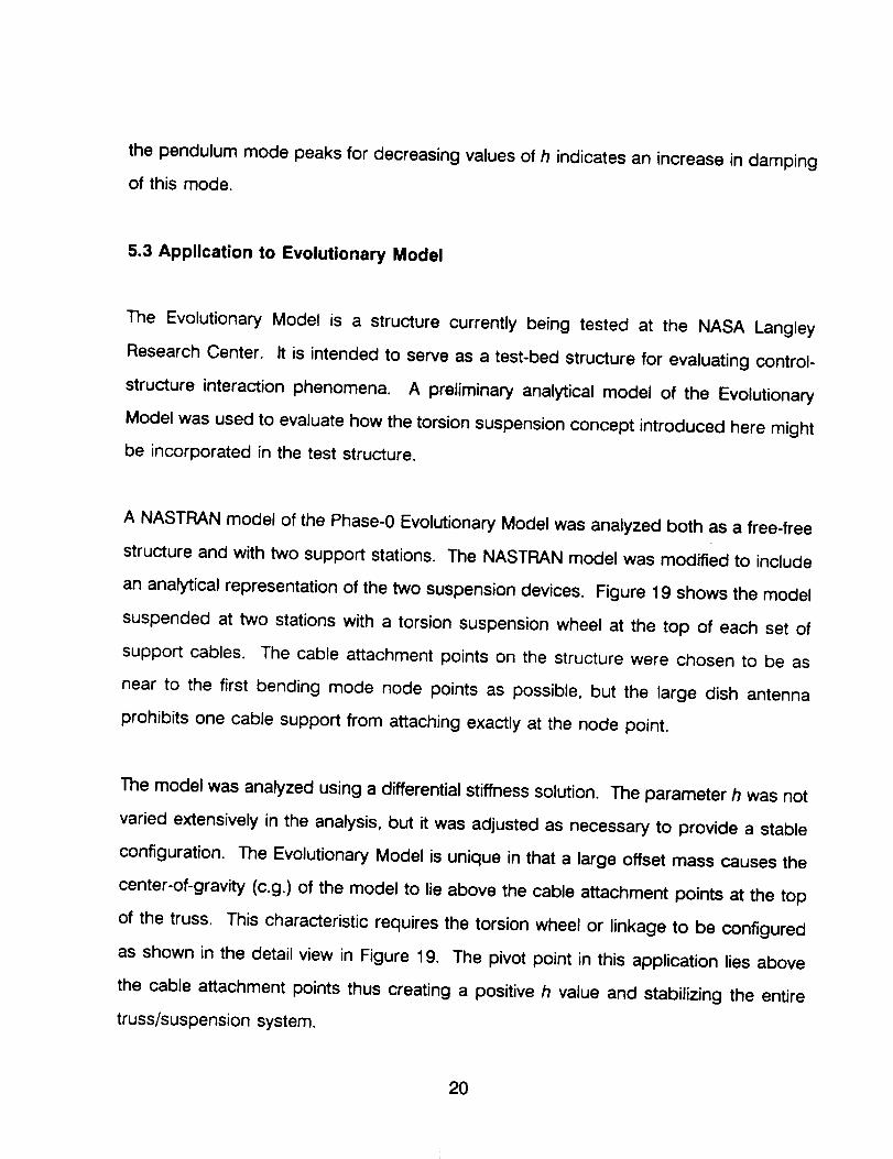
5.3 Application to Evolutionary Model
The Evolutionary Model is a structure currently being tested at the NASA Langley
Research Center. It is intended to serve as a test-bed structure for evaluating control-
structure interaction phenomena. A preliminary analytical model of the Evolutionary
Model was used to evaluate how the torsion suspension concept introduced here might
be incorporated in the test structure.
A NASTRAN model of the Phase-0 Evolutionary Model was analyzed both as a free-free
structure and with two support stations. The NASTRAN model was modified to include
an analytical representation of the two suspension devices. Figure 19 shows the model
suspended at two stations with a torsion suspension wheel at the top of each set of
support cables. The cable attachment points on the structure were chosen to be as
near to the first bending mode node points as possible, but the large dish antenna
prohibits one cable support from attaching exactly at the node point.
The model was analyzed using a differential stiffness solution. The parameter h was not
varied extensively in the analysis, but it was adjusted as necessary to provide a stable
configuration. The Evolutionary Model is unique in that a large offset mass causes the
center-of-gravity (c.g.) of the model to lie above the cable attachment points at the top
of the truss. This characteristic requires the torsion wheel or linkage to be configured
as shown in the detail view in Figure 19. The pivot point in this application lies above
the cable attachment points thus creating a positive h value and stabilizing the entire
truss/suspension system.
20
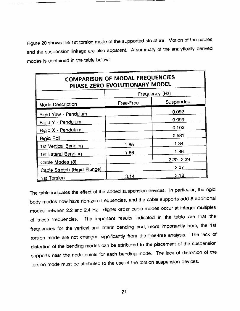
Figure 20 shows the 1st torsion mode of the supported structure. Motion of the cables
and the suspension linkage are also apparent. A summary of the analytically derived
modes is contained in the table below:
COMPARISON OF MODAL FREQUENCIES
PHASE ZERO EVOLUTIONARY MODEL
Mode Description
Rigid Yaw - Pendulum
Rigid Y - Pendulum
Rigid X - Pendulum
Rigid Roll
1st Vertical Bending
1st Lateral Bending
Cable Modes (8)
Cable Stretch (Rigid Plunge)
1 __t Torsion
Frequency (Hz)
Free-Free Suspended
0.092
0.099
0.102
0.581
1.85 1.84
1.86 1.86
2.20- 2.39
3.07
3.183.14
The table indicates the effect of the added suspension devices. In particular, the rigid
body modes now have non-zero frequencies, and the cable supports add 8 additional
modes between 2.2 and 2.4 Hz. Higher order cable modes occur at integer multiples
of these frequencies. The important results indicated in the table are that the
frequencies for the vertical and lateral bending and, more importantly here, the 1st
torsion mode are not changed significantly from the flee-free analysis. The lack of
distortion of the bending modes can be attributed to the placement of the suspension
supports near the node points for each bending mode. The lack of distortion of the
torsion mode must be attributed to the use of the torsion suspension devices.
21
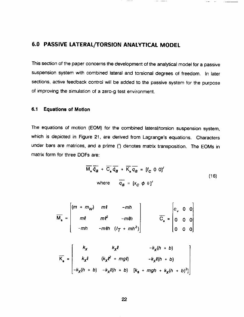
6.0 PASSIVE LATERAL/TORSION ANALYTICAL MODEL
This section of the paper concerns the development of the analytical model for a passive
suspension system with combined lateral and torsional degrees of freedom. In later
sections, active feedback control will be added to the passive system for the purpose
of improving the simulation of a zero-g test environment.
6.1 Equations of Motion
The equations of motion (EOM) for the combined lateral/torsion suspension system,
which is depicted in Figure 21, are derived from Lagrange's equations. Characters
under bars are matrices, and a prime (') denotes matrix transposition. The EOMs in
matrix form for three DOFs are:
M o Ela + Ca <fla * K'a__a = [fc 0 0]'
n
where qa = [Xc #_ e] I
(16)
Ma
(rn + row) m_ -mh
mO mr7 -m_
-mh -m_ (I T + mh 2)
c v 0 O]
000 0
kx
kx_ (kx_ + mg_)
-kx(h + b) -kxO(h + b) [k 8
-kx(h + b)
-kxO(h + b)
+ mgh + kx(h + b) 2]
22
The definitions of the notations in Eq. 16 are:
g = 386.4 in/s 2, acceleration due to gravity
mg = 99.48 Ib, weight of the test structure
m, = 2/g Ib-sZ/in, mass of the wheel (3-bar linkage) and cart
/ = 1,777/g Ib-s2-in, c.g. moment of inertia of the test structure
I, = 338/g Ib-sZ-in, moment of inertia of the wheel (3-bar linkage) about its c.g.
IT= I + I,
= 88.625 in, cable length
b = 3.00 in, distance above the spring elastic center of the test structure's c.g.
kx = 0.756 Ibs/in, horizontal-translation spring constant
k e = 194.5 Ib-in/rad, rotational spring constant
c v = viscous damping constant representing friction of the linear bearing
h = h 1 - h 2 (see Fig. 21), a variable parameter
fc = feedback-control force
x c = cart translation DOF
= rotation angle of the cables
e = rotation angle of the test structure
Note that the values listed match those of the experimental test apparatus described in
section 2.0. A viscous damping matrix with one non-zero damping constant c,, has been
added to approximate the friction of the linear bearing. Estimation of c,, based on
measured response of the system is described in Section 4.4.
In later considerations of closed-loop control of horizontal motion, translations of the
wheel-cart and the test structure are the measured quantities used as input to the
control system. It is appropriate, therefore, to replace the rotations in Eq. 16 with
translations, and two reasonable quantities to use are x o, translation of the test structure
23

c.g., and Xe, translation of the elastic center of the external spring system, as illustrated
on Figure 21. Hence, we define a new set of DOFs, qb = [Xc Xo Xe] I The
transformation between the two sets of DOFs is
qa = T qb (17)
w
T=
1 0 0
1 h+b h
_b _b
1 1
b b
Hence, we transform the original mass, damping and stiffness matrices with the matrix
product Mbb = _ M T , etc. Then the EOMs in the second set of DOFs are
MbClb + C bclb + Kb qb = [fc 0 0] / (18)
Mb
m w
0
0
0 0
IT I T
Cm+
IT I T
b 2 b 2
24
Kb
mg mg h + b
Q Q b
_ + (j + m_
b b bb
b b z _ b b
mg h
Q b
b b
kX+ b2+ 0 b +
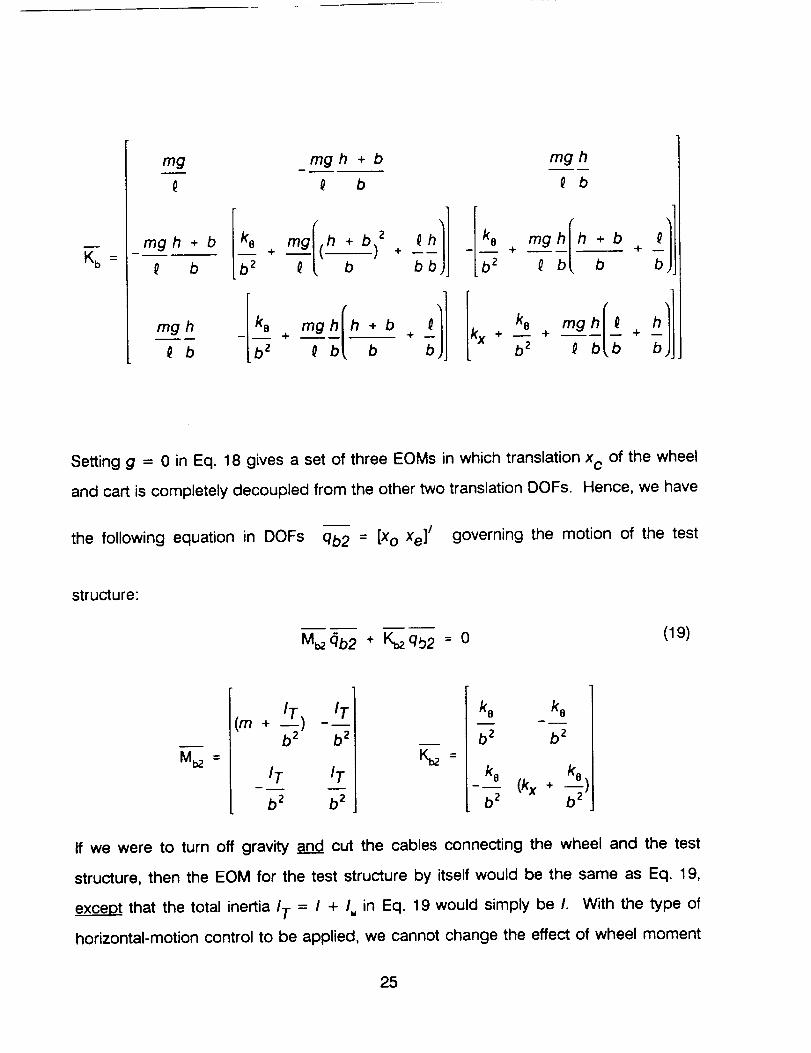
Setting g = 0 in Eq. 18 gives a set of three EOMs in which translation x c of the wheel
and cart is completely decoupled from the other two translation DOFs. Hence, we have
the following equation in DOFs qb2 = [Xo Xe ]/ governing the motion of the test
structure:
M_. Clb2 + K_ q_2 = 0(19)
M_
(m ÷ IT)b 2
IT
b 2
IT
b 2
K=
k s kea
b z b z
If we were to turn off gravity and cut the cables connecting the wheel and the test
structure, then the EOM for the test structure by itself would be the same as Eq. 19,
excep__ that the total inertia I T = I + I,, in Eq. 19 would simply be I. With the type of
horizontal-motion control to be applied, we cannot change the effect of wheel moment
25
of inertia I W. Hence, the modes of Eq. 19 should be considered the target modes for the
controlled system, even though I. is not present in the O-g EOMs of the test structure
by itself. (It is interesting to note that, in principle, I. could be canceled if it were
possible to implement a rotational acceleration feedback control on the wheel.)
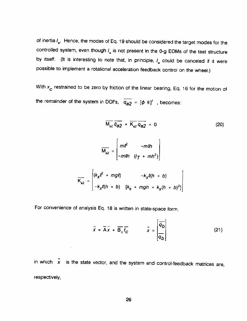
With x c restrained to be zero by friction of the linear bearing, Eq. 16 for the motion of
the remainder of the system in DOFs, qa2 = [¢) 0]_ , becomes:
M.z lfla2 + K-_J2_a2 = 0 (20)
Ma2 =
_ I(kx_ +mgO)= -kxO(h + b) lK"2 [-kxO(h + b) [k 8 + mgh + kx(h + b) z]
For convenience of analysis Eq. 18 is written in-state-space form,
x = Ax + Bcf c x = (21)
in which x is the state vector, and the system and control-feedback matrices are,
respectively,
26
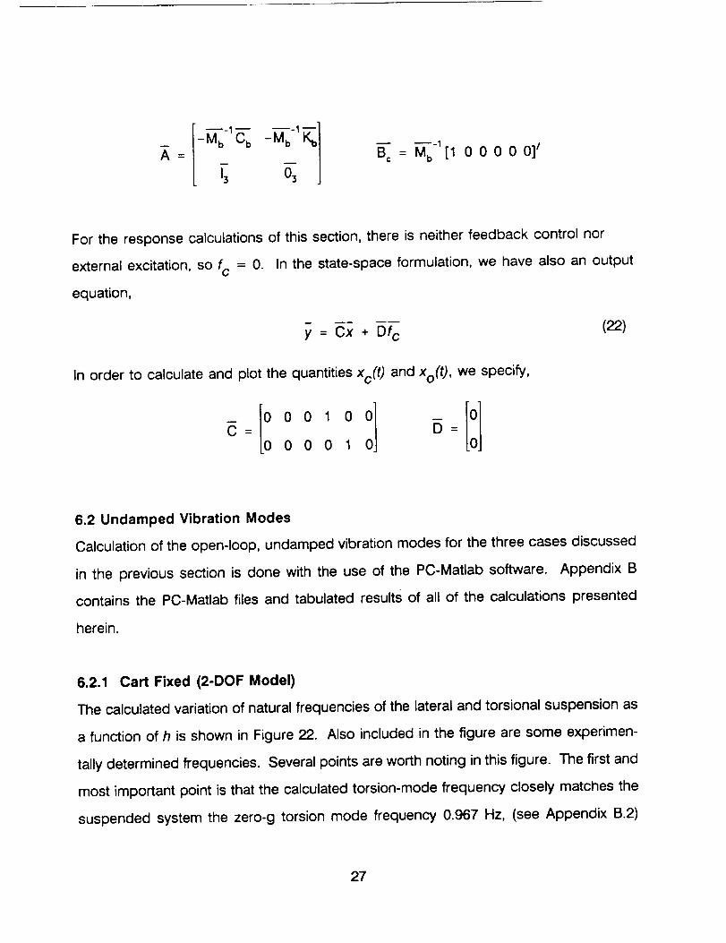
A=-Mb Cb -Mb KbI _ = M-'bb-'
[1 0 0 0 0 0] I
For the response calculations of this section, there is neither feedback control nor
external excitation, so fc = 0. In the state-space formulation, we have also an output
equation,
y = Cx + Df c (22)
In order to calculate and plot the quantities Xc(t) and Xo(t ), we specify,
I:oo 0c;ooo :l6.2 Undamped Vibration Modes
Calculation of the open-loop, undamped vibration modes for the three cases discussed
in the previous section is done with the use of the PC-Matlab software. Appendix B
contains the PC-Matlab files and tabulated results of all of the calculations presented
herein.
6.2.1 Cart Fixed (2-DOF Model)
The calculated variation of natural frequencies of the lateral and torsional suspension as
a function of h is shown in Figure 22. Also included in the figure are some experimen-
tally determined frequencies. Several points are worth noting in this figure. The first and
most important point is that the calculated torsion-mode frequency closely matches the
suspended system the zero-g torsion mode frequency 0.967 Hz, (see Appendix B.2)
27
when h = 0. The rightward shift of the experimental points from the predicted curve is
believed to be due to uncertainties in measurement of the effective cable attachment
points in determining h. Because of cable stiffness effects, the cable end attachment
points may not behave as perfect hinges as was assumed. Also note that the lateral
mode frequency for this case with cart fixed is the simple pendulum frequency, 0.426 Hz,
versus 0.265 Hz for zero-g (see Appendix B.2) and is insensitive to changes in h within
the h range of practical interest.
6.2.2 Cart Free (3-DOF Model)
This is a useful theoretical case, even though it is not physically realizable due to the
substantial friction in the linear bearing. The calculated results for this case are given
in Appendix B.3, and the natural frequencies are plotted in Figure 23. Comparison of
the results in Figure 23 with those in the previous figure shows that by freeing the cart
the lowest two modes of the undamped 3-DOF model for h = 0 are nearly identical to
the modes of the 0-g, 2-DOF test structure. Hence, if the linear bearing were frictionless,
then the passive cable-suspension system described by the model with h -- 0 would do
an excellent job of simulating the 0-g case. It appears, then, that the primary function
of the active horizontal-motion control system is to compensate for the friction in the
linear bearing by forcing the wheel-cart to move as if the bearing were frictionless. In
order to design such a control system, we must know at least the order of magnitude
of the friction (as represented by the parameter c,,), and this issue is addressed in the
next section.
6.3 Damped Vibration Modes
The experimental result suggests that the linear bearing's friction has a complex nature,
probably much more like Coulomb friction than viscous damping. However, use of the
linear analysis capabilities of PC-Matlab requires that the damping model be linear, so
28
the objective of the exercise described here was to infer a linear viscous damping
constant c v that influences the dynamic response in a fashion similar to the actual
bearing friction.
The resonant driving and release is simulated by a simple initial-condition, with zero
external excitation: the initial velocity has the shape of the undamped 3-DOF translation
mode, and the initial displacement is zero. The subsequent time-history of response is
calculated and plotted for a specified value of c v.
In the time-history graphs to be discussed next, Xc(t) is plotted with solid lines, and Xo(t)
is plotted with dot-dash lines. The first case is for c v = 0 Ib/ips, and it is a check on the
functioning of the PC-Matlab solution (veloresp.m in Appendix B.4); the results are
plotted on Figure 24a. The response is free, undamped vibration in the translation mode
at 0.265 Hz of the 3-DOF model, in perfect agreement with the h = 0 modal results of
Appendix B.2. This result tends to validate that veloresp.m is functioning correctly.
The other cases are for cv = 0.1, 1.0, 10 and 100 Ib/ips, and the results are plotted on
Figures 24b, 24c, 24d, and 24e, respectively. For c, = 0.1 Ib/ips, the damping appears
to be proportional and modal in the 0.265 Hz mode of the 3-DOF model. For c_ = 1.0
Ib/ips, the damping appears to be nonproportional, which indeed it is, and the character
of the response is quite different from that of the 0.265 Hz mode. For c,, = 10 Ib/ips,
motion x c of the cart is very small, and motion x o of the test structure is only lightly
damped at a frequency almost indistinguishable from 0.426 Hz, the h = 0 translation
mode frequency of the 2-DOF model with fixed cart. Finally, for c,, = 100 Ib/ips, x c is
almost completely suppressed, and x o is in free vibration at 0.426 Hz with almost
imperceptible damping.
29
7.0 ACTIVE CONTROL OF LATERAL_rORSION SUSPENSION
7.1 General Design Considerations
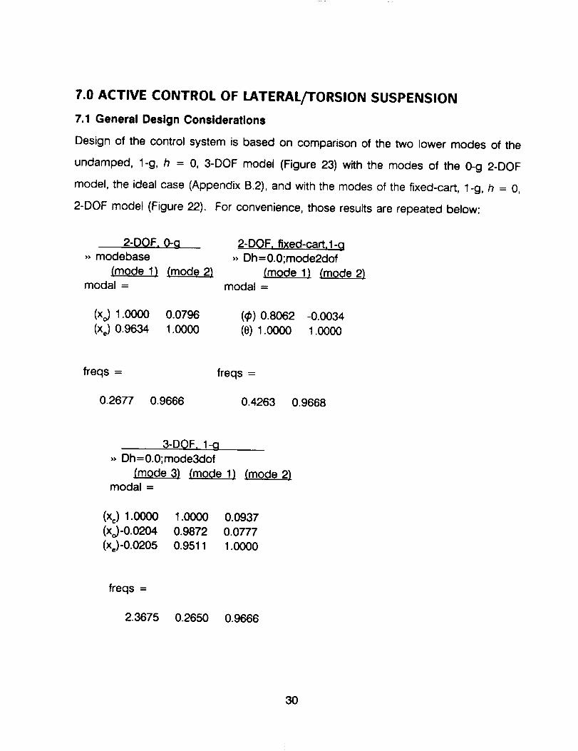
Design of the control system is based on comparison of the two lower modes of the
undamped, l-g, h = 0, 3-DOF model (Figure 23) with the modes of the 0-g 2-DOF
model, the ideal case (Appendix B.2), and with the modes of the fixed-cart, l-g, h = 0,
2-DOF model (Figure 22). For convenience, those results are repeated below:
2-DQF, 0-g- modebase
(mode 1) (mode 2)modal =
(xo) 1.0000 0.0796
(xe)0.9634 1.0000
2-DOF. fixed-cart, 1-g
- Dh=0.0;mode2dof
(mode 1) (mode 2)modal =
(9) 0.8062 -0.0034(e) 1.0000 1.0000
_eqs =
0.2677 0.9666
freqs =
0.4263 0.9668
3-DOF, 1-g
- Dh =0.0;mode3dof
(mode 3) (mode 1)modal =
(mode
(xc) 1.0000 1.0000 0.0937
(xo)-0.0204 0.9872 0.0777
(Xe)-0.0205 0.9511 1.0000
freqs =
2.3675 0.2650 0.9666
30
Mode 2 is essentially the same in all three cases, which shows that setting h = 0 in the
1-g cases is an effective passive method for preserving the 0-g rotation mode. Active
control is required, therefore, only to preserve the 0-g translation mode, mode 1, in the
environment of 1-g and the sticky linear bearing.
Observe in 3-DOF mode 1, the translation mode, that xc _ x o, which means that the cart
remains almost directly above the test structure's c.g. This suggests that the control
system for the actual damped laboratory article should, for motion in the translation
mode, maintain the cart directly above the test structure's c.g. Cart position xc can be
sensed with a potentiometer. Likewise, position of the test structure can be sensed with
a noncontacting Kaman transducer, but xo is not the test structure translation that should
be sensed. The nodal point of 3-DOF mode 2, the rotation mode, is not right at the c.g.,
but rather a short distance above it. Therefore, sensing of xo could cause the control
system to modify the rotation mode, which would probably be counterproductive.
It is appropriate, therefore, to sense the translation of the test structure at the nodal point
of the 3-DOF rotation mode, which is a distance d above the spring elastic center. The
translation of the nodal point is denoted xd and is given in terms of the defined DOFs
by
31

x d = x e + dO X°Xel= xe + = x ob + Xell
The ratio d/b is found from the shape of 3-DOF mode 2 to be
(1 -Xo/Xe)l = (1 -0.0777) 1 = 1.0843.
(23)
It has been established that the control system should maintain x c = x d in order to
preserve the O-g translation mode with minimal effect on the rotation mode. Accordingly,
we define the error quantity
E = Xd - Xc = C_x
where, from Eqs. 21 and 23, the output matrix is
(24)
C--_ : 000-1 ;(25)
We consider in subsequent sections methods for effecting control by making control
force fc a linear function of E, and/or its time integral, and/or its time derivative. These
types of control are commonly called proportional (P), integral (I), and derivative (D)
control, and combinations thereof are referred to as PD, PID, etc. control.
32
7.2 Proportional Control
For proportional control, we define the feedback constant Cp
fc(t) = Cp _.(t)
Combining Eqs. 21,24-26 then gives
and set
(26)
x = (A + CpB cC,)x = AcX (27)
The matrices A, B c and _ can be calculated by specifying h (= 0 in the
following), c,, and d/b (= 1.0843 in Appendix Bo5) and running the PC-Matlab m-file (see
Appendix B.5). The effect of varying the proportional feedback constant Cp on the lateral
mode eigenvalues is shown in Figure 25. For this case the damping constant c v = 1.0
was assumed. Note the similarities between this figure and Figure 14, the open-loop
case where the damping constant cv was varied. The root loci are essentially the same
in both figures, demonstrating that active control of the cart's lateral position relative to
that of the suspended body effectively compensates for the adverse effects of cart
damping with regard to simulating 0-g test conditions.
33
For all of the cases discussed to this point, the 0-g vibration modes of the test structure
involve structural deformation and therefore have positive natural frequencies. There is
interest also in the case for which the structure is not restrained by springs and therefore
has at least one zero-frequency rigid-body mode in 0-g. For this case, then, we let
stiffness constants k, and k e be zero. To avoid the complication of repeated zero
eigenvalues, we consider h > 0. In particular, we evaluate the case with numerical
values h = 1.75, mg = 100 Ib, m,g = 5.65 Ib, _ = 62.125", with all other values the
same as before. Changing these values in PC-Matlab and running the modified m-file
(under the name k0mde3df.m) gives the following for the undamped, 1-g modes:
$-DOF, l-g, Unrestrained
,, Dh = 1.75;k0mde3df
(xc)
(xj
(mode 3) (mode 1) (mode 2)modal =
1.0000 1.0000 -0.7273
-0.0565 1.0000 0.0411
-0.0372 1.0000 1.0000
freqs =
1.7255 0.0000 0.8952
The translation mode now is a zero-frequency rigid-body mode, and the rotation mode
has 0.8952 Hz natural frequency.
The modes above are for zero friction in the linear bearing. When c v increases slightly
above zero, then the rigid-body translation mode remains at zero frequency but has an
exponential damping time constant. It is not appropriate, therefore, to plot the locus of
34
roots in the frequency vs. zeta form used for Figures 14 and 25. Accordingly, the
appropriate m-files have been modified to calculate and plot loci of roots in the more
traditional form of imaginary part vs. real part (see Appendix B.6).
The open-loop results for c,, varying 0-0.4 Ib/ips are shown in Figure 26. There are three
ranges of c,, in which the roots are qualitatively different: 0 to about 0.29, about 0.29 to
about 0.36, and above about 0.36 Ib/ips. In the middle range, the only oscillatory roots
are those of the rotation mode.
The results of Figure 25 establish that proportional control tends to achieve the desired
effect if the translation mode has positive natural frequency. The question now is
whether or not proportional control performs as desired also for the zero-frequency
modei i.e., does proportional control move the roots of the rigid-body translation mode
of Figure 26 toward the origin, decreasing the damping in that mode and making it
appear more like the true undamped, 0-g mode? To answer this question, the closed-
loop case is also modelled in Appendix B.6. The results are presented in Figures 27a
thru 27c. In each figure, c,, is assigned a value and proportional feedback constant Cp
is varied 0-2 Ibs/in in increments of 0.1 Ibs/in. In each case, proportional control forces
the translation mode's roots toward the origin, which is the desired effect.
7.3 Proportional-Integral-Derivative Control
For general PID control, we define feedback constants Cp, C i and C d, and then express
the control force as
35
tc = cp + Ci[otC(o)do+ C v(t) (28)
The derivative term in Eq. 28 requires some explanation. It is not possible or even
desirable in practice to implement an exact derivative operation, so a standard alternative
procedure is to introduce a new variable v(t) and to approximate the derivative with a
single-pole high-pass filter,
_'d _ + v = _(t) (29)
For small values of time constant Td, we have v = de/dt for low-frequency c(t) signals
and v = e/-rd for high-frequency signals. Hence, choosing "ra appropriately results in a
good approximate differentiation of low-frequency signals of interest without the
undesirable differentiation of high-frequency noise. (A band-pass filter with appropriate
parameters would be an equally accurate differentiator and a more effective noise
attenuator, but it would increase the order of Eq. 29 and, hence, the number of states
in the controller.) For example, setting "rd = 0.025 sec gives an approximate differentia-
tor that is accurate to less than 9 o of phase error and 1% of magnitude error for signals
of 1 Hz or lower.
It is necessary now to write Eqs. 28 and 29 in a state-space form. To do so, we define
the controller state variables,
Error signal c(t) is the input to the controller. Then the definition of z 1 and the integral
of Eq. 29, with the definition of z 2, constitute the controller state equations,
36
(31)
Equation 29, the controller output equation, becomes
= ÷(32)
CdDz = Cp +
T d
Finally, we combine Eqs. 21, 24, 31 and 32 to obtain the state equation of the entire
closed-loop system, which consists of both the laboratory structure and the dynamic PID
controller:
I(x-+O,B C,)B,C, Azz
(33)
The roots of Eq. 33 are evaluated by three PC-Matlab m-files (see Appendix B.7). These
files generated results which allow a quick assessment of the effects of derivative and
integral feedback on the basic proportional-control system. The results are shown on
Figure 28. The root loci on Figure 28 suggest that derivative and integral feedback are
not very helpful and that simple proportional feedback is the most effective. This,
however, is a cursory evaluation, and a more detailed analysis would be required to
determine with certainty the relative merits of proportional, integral, and derivative
feedbacks in this control problem.
37
7.4 Experimental Results
To evaluate the analytical results described in the previous sections, the lateral
suspension system was supplemented with an active feedback control system. As
pictured in Figure 6, the "moving cart" was attached to a drive belt and driven by a small
DC motor. The absolute position of the cart was read by a potentiometer directly driven
by the belt/motor.
In Section 7.1 the error signal, c, was derived as the difference of the cart absolute
position and the test structure's absolute position measured at the nodal point of its 3-
DOF rotation mode. To implement this error as a feedback control signal, the test
structure described in Section 2.0 was instrumented with a Kaman non-contact
displacement probe at a point near the node of the rotation mode. The use of the non-
contact probe allowed sensitive displacement measurements to be made without adding
friction to the system. However, the non-contact probe provides linear output over a
maximum range of two inches. This limit did not prohibit the evaluation of the active
control technique, but, in order to achieve even the two inch range, the largest diameter
(also two inches) non-contact probe was required. This large diameter did not allow
displacement measurement at precisely the rotation mode nodal point. Instead, the
displacement over a much larger area was sensed and averaged thus introducing effects
of the rotation mode.
The active control system was implemented with a digital controller made by Spectrum
Signal Processing. This IBM-PC compatible controller card utilizes a Texas Instruments
(TI), TMS320C25 Digital Signal Processing (DSP) microprocessor to allow high
throughput rates and extremely fast data processing rates. This card is supplemented
by an additional input/output (I/O) card to provide four simultaneous sampling input
38
channels. Each channel provides 12 bit analog-to-digital (A/D) conversion at sample
rates up to 58 kHz. The I/O card also provides two output channels. It is apparent that
the high sample rates and indeed even the digital controller are not required to
implement such a simple control algorithm, but the system can be expanded to provide
multiple control loops for several suspension devices. As such, a high speed, high data
throughput system was purchased for evaluation. Once setup, the digital controller also
allows very easy implementation of new control laws or the inclusion of derivative or
integral feedback as described earlier.
The proportional control scheme as described in Section 7.2 was implemented in the
controller. The assembly language listing of the control algorithm is shown in Appendix
C. The two previously calibrated, absolute position measurements were read by the A/D
inputs of the I/O card. The difference of the two signals was taken to obtain the error,
(. The error was multiplied by a gain and output by the I/O card. The lateral
suspension motor was driven by the output signal after being amplified and conditioned
by a servo amplifier.
Results of this simple evaluation were disappointing. Rather than providing a smoothly
operating suspension system which follows the motion of the test structure, the motor
was driven into a relativelyhigh frequency, limit-cycle oscillation. This result was clearly
not predicted by the earlier analyses. The oscillations were not difficult to account for
after a simple examination of the system. The oscillations were occurring at a frequency
of approximately 2 Hz, clearly above the lateral frequency of the test structure, but
closely matching the cart mode frequency. The cart mode response was greatly
enhanced by the additional mass and dynamics of the vertical suspension system which
also has structural system modes at approximately 2 Hz. This enhanced response and
39
the vertical suspension dynamics were being sensed by the potentiometer and fed back
into the error signal, thus driving the system unstable.
A consideration was given to try to filter the feedback signals. However, to achieve the
large rolloff in frequency desired to eliminate the spurious mode response, a sharp (80
dB/oct) filter is necessary. Such filters were available but were also found to have phase
shifts at 0.3 Hz as large as 60 degrees. Such large phase shifts in the controller
bandwidth are not acceptable and the technique had to be abandoned.
It was felt that simplifying the hardware of the complete test apparatus would provide a
better evaluation of the method. Unfortunately, it was not possible to include this
alternative approach within the current effort. Thus, the experimental results for the
active system remain inconclusive.
8.0 CONCLUDING REMARKS
Exploratory studies have been conducted for very low frequency suspension systems
for dynamic testing of large, flexible space structures. An experimental 3 DOF
suspension apparatus supporting a simulated large space structure has been analytically
modelled, fabricated and tested. The characteristics of the passive lateral suspension
system augmented with active feedback control was also studied.
Conclusions drawn from the results of these analytical and experimental studies include:
• The ZSRM provided minimum vertical mode suspension frequencies below 0.1
Hz and allowed a maximum travel of +/- 3 inches.
40
, The torsion suspension concept introduced in this report is effective in simulating
unconstrained conditions for the first torsion mode of beam-like structures.
,For the lateral suspension system, damping and friction forces in the moving cart
mechanism (a linear bearing) severely limited the ability of the system to simulate
zero-gravity conditions.
. Analytical studies indicated that active proportional feedback control of the
moving cart would eliminate the adverse effects of damping identified during
tests of the lateral suspension system. Attempts to experimentally demonstrate
active augmentation of the 3 DOF suspension test apparatus were not
successful, however, due to dynamic instabilities resulting from coupling of the
higher frequency spurious modes of the overall system.
o The digital control card used in the active control implementation was found to
have extensive capability and would be suitable for control of several control
loops for multiple suspension devices. However, the interface to the controller
requires programming in TI assembly language thus entailing extensive time for
familiarization. Furthermore the DSP chip on the controller card is limited to
fixed-point arithmetic which further complicates the programming. For future
applications, newer, floating-point arithmetic DSP chips are now available (at
much higher cost) and offer alternative operating system environments to ease
some of the interfacing difficulties.
41
9.0 REFERENCES
,
o
Kienholz, D.A., Crawley, E.F., and Harvey, T.J.: '_/ery Low Frequency Suspension
Systems For Dynamic Testing". AIAA Paper 89-1194, Proc. 30th Structures,
Structural Dynamics, and Materials Conference, Mobile, AL, April 1989.
Gold, Ronald R., Reed, Wilmer H., II1: "Preliminary Evaluation of SuspensionSystems for 60-Meter MAST Flight System". DEI Report. No. C2602-008,
February 1987.
42
APPENDIX A
SUSPENSION SYSTEM ASSEMBLY PROCEDURE
By Edward Y. Brandt
Included in this Appendix are instructions for the assembly and installation of the
experimental suspension system. The procedures should be followed carefully to avoid
damage to the system and for safety reasons. Proper assembly of the system requires
the presence of two persons. The necessary tools include open ended wrenches (3/8,
7/16, 1/2 inch) and a set of allen wrenches. A drawing of the complete assembly is
shown in Figure 6. This drawing identifies the components which are discussed in the
assembly procedures.
I. ASSEMBLY
A°The lateral system, including the linear bearing assembly, motor, potentiometer,
gears and drive belt should be installed first. The aluminum bar on which the
linear bearing assembly rests must be supported at either end at a height of at
least 13 feet from the floor. It is important that the bar is level.
goWith the lateral system in place, the vertical system can be assembled and
mounted to the lateral system by the following procedures:
,Attach the upper and side plates of the vertical system mounting box to the
linear bearing block, then connect the lower mounting plate and the horizontal
support member.
43
.
Insert the upper flexure assemblies into the ends of the horizontal support
member and bolt in place.
NOTE: There are four holes in two of the flexure blocks for flexure length
adjustment. For the current configuration the bolt must go through the third hole
from the inboard end to make the vertical members parallel.
.
Slip the vertical members onto the flexure blocks and bolt into place.
,
Insert the threaded rod through the horizontal support member and lower
mounting plate. Secure in place with two nuts, one above and one below.
.
Slide the main spring attachment plate onto the threaded rod and secure with
a nut.
NOTE: The location of the plate along the threaded rod will vary greatly
depending on the amount of weight being supported and the size of the main
springs being used.
.
Attach the eyebolts to the plate and hang main springs.
NOTE: If more extension of the main springs is required, remove the threaded
rod and attach the eyebolts directly to the lower mounting plate. By doing so
the length of the main springs will increase with a Y(_ss of adjustment travel.
°
With the weight box supported, hang the lower subassembly on the main springs
from the eye bolts. This lower subassembly includes the center linkage
members, the center and side flexures, the torsion suspension assembly, the
cables and the weight box.
44

.Remove the support and add weights to the box until the desired weight is
attained.
.With the desired weight in the weight box, adjust the main spring position on the
threaded rod so that the lower horizontal members can be attached to the
bottom of the vertical members. If more adjustment is needed, adjust the
eyebolts evenly.
10. Slide the side spring mounting brackets up the vertical member and secure them
about three inches up the tube.
11. Connect the vertical members to the lower horizontal members with the lower
flexure assemblies. The vertical motion stops are also installed at this time as
they share a common bolt.
12. Adjust the main spring tension until the lower horizontal members are level.
13. Allow the side spring mounting brackets to rest on the backplates. Attach
eyebolts to the bracket opposite the force gage with the eyebolts in their most
extended position.
14. Attach the eyebolts to the side spring attachment bar in their most extended
position and connect side springs.
15. Grasp the bar firmly while supporting the structure and stretch the springs until
the center hole engages on the force gage stud. A second person should
45
secure the vertical members and secure the spring attachment bar on the stud
with a nut.
16.Increase the extension/pretension of the side springs by adjusting the side eye
bolts and the nut securing the spring attachment bar. The side spring
pretension can be set to the proper level using the force gauge. Minor
adjustments will be required on the main spring tension during this process in
order to center the system.
II. PROCEDURES FOR CHANGING THE SYSTEM WEIGHT
A,
Never attempt to remove or add weight to the box without securing the box
firmly in a fixed position. The vertical motion stops are not designed to withstand
the force of the main springs. If the weight is removed without the proper
precautions, the three lower flexures will be damaged and will need to be
replaced.
g.
An alternative to securing the weight box in a fixed position is to disassemble the
lower portion of the system using this procedure:
1. Loosen side spring tension at all four eyebolts.
.
Remove the side spring attachment bar from the force gage stud.
second person remove the nut and help support the structure.
Have a
3. Remove one of the eyebolts from the bar to allow springs to hang.
46

4. Remove flexure blocks and vertical motion stops.
5. Reload box to desired weight.
6. Adjust the position of the main springs to set the correct vertical position of lower
horizontal members.
7. Re-assemble in reverse order.
47

APPENDIX B.1
2-DOF Model of Full System in 1-g with Cart Fixed
A PC-Matlab m-file called hz2dof.m calculates and plots the natural frequencies of Eq.
20 versus the parameter h (denoted Dh in all m-files). The m-file is:
%hz2dof.m mod 1 2/2/90 To calc and plot nat freqs of 2-dof dei model.
%First calc mass & stiffness matrices (ref. Gold's derivation & my
%10/27/89 re-derivation), then calc the nat freqs in Hz.
%Required input is Low, Inc, Hii for Dh=Low:lnc:Hii.
%Output is a plot of the two nat freqs versus Dh, which is hl-h2.
M g = 99.48;g = 386.4; M = Mg/g; Mw = 2/g ;Iw = 338/g;I = 1777/g;
Kx= .756;Kt = 194.5;b = 3;L=88.625;
j=0;for Dh = Low: Inc: Hii
j=j+l;
Dhb=Dh+b;mas2=[M*L ^ 2 -M*L*Dh;-M*L*Dh lw+l+M*Dh ^ 2];
stf2= [Kx*L ^ 2+ Mg*L -Kx*L*Dhb;-Kx*L*Dhb Kt+ Mg*Dh + Kx*Dhb ^ 2];
Hz= (eig(stf2,mas2). ^ .5)/(2"pi);
H(j) = Dh;Freqs(j,1:2) = [Hz(1 ) Hz(2)];end
plot(H,Freqs(:,l),H,Freqs(:,2),'--'),grid,ylabel('FREQUENCY in Hz'),
xlabeI('DELTA-H in inches'),
title('NATURAL FREQUENCIES OF DEI 2-DOF MODEL')
The user runs hz2dof.m in PC-Matlab by first defining Low, Inc, and Hii, which are the
low value, increment, and high value, respectively, of h, and then typing the m-file name,
hz2dof. M-file hz2dof.m generates a plot, Figure 22, of the two undamped natural
frequencies (in Hz) versus h.
The mode shapes for this case are also of interest, so a separate m-file, mode2dof.m,
was written to calculate them:
%mode2dof.m 2/2/90 Calc modes of 2-dof cable- and spring-supported
48
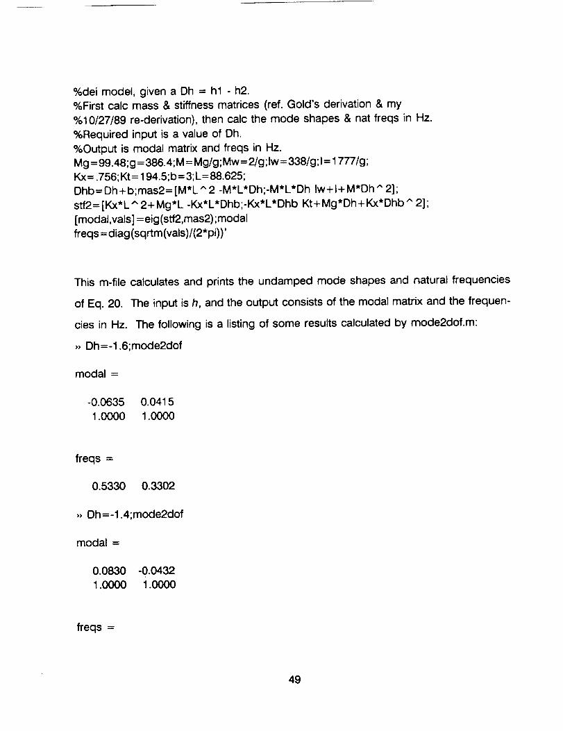
%dei model, given a Dh = hl - h2.%First calc mass & stiffness matrices (ref. Gold's derivation & my%10/27/89 re-derivation), then calc the mode shapes & nat freqs in Hz.%Required input is a value of Dh.%Output is modal matrix and freqs in Hz.Mg= 99.48;g =386.4;M= Mg/g;Mw= 2/g ;Iw= 338/g ;I= 1777/g;Kx=.756;Kt= 194.5;b=3;L=88.625;Dhb= Dh+b;mas2--- [M*L ^ 2 -M*L*Dh;-M*L*Dh Iw+l+ M*Dh ^ 2];stf2= [Kx*L ^ 2+ Mg*L -Kx*L*Dhb;-Kx*L*Dhb Kt+ Mg*Dh+ Kx*Dhb ^ 2];[modal,vals] = eig(stf2,mas2);modalfreqs= diag (sqrtm(vals)/(2*pi))'
This m-file calculates and prints the undamped mode shapes and natural frequencies
of Eq. 20. The input is h, and the output consists of the modal matrix and the frequen-
cies in Hz. The following is a listing of some results calculated by mode2dof.m:
,, Dh=-1.6;mode2dof
modal =
-0.0635 0.0415
1.0000 1.0000
freqs =
0.5330 0.3302
)) Dh=-1.4;mode2dof
modal =
0.0830 -0.0432
1.0000 1.0000
freqs =
49
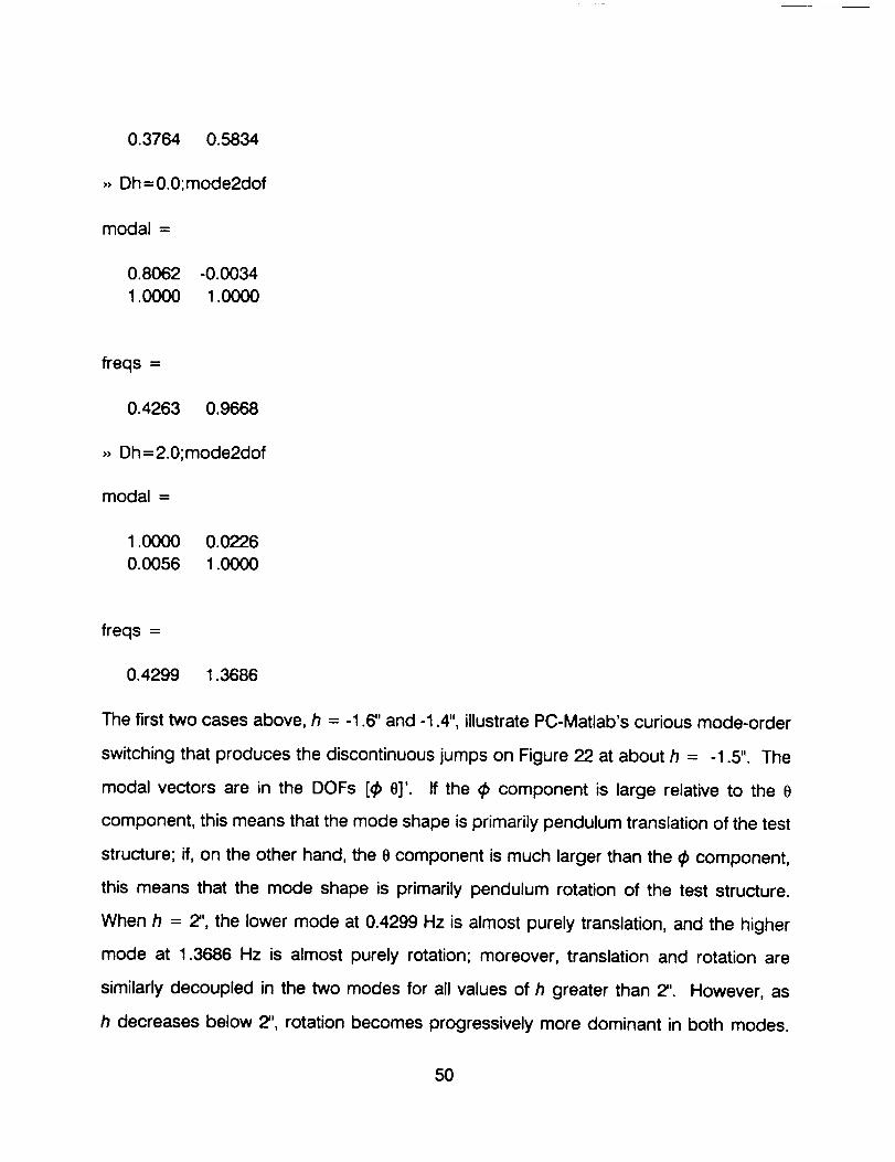
0.3764 0.5834
,, Dh=0.0;mode2dof
modal =
0.8062 -0.0034
1.0000 1.0000
freqs =
0.4263 0.9668
,, Dh=2.0;mode2dof
modal --
1.0000 0.0226
0.0056 1.0000
freqs =
0.4299 1.3686
The first two cases above, h = -1.6" and -1.4", illustrate PC-Matlab's curious mode-order
switching that produces the discontinuous jumps on Figure 22 at about h = -1.5". The
modal vectors are in the DOFs [4 e]'. If the _ component is large relative to the e
component, this means that the mode shape is primarily pendulum translation of the test
structure; if, on the other hand, the e component is much larger than the (_ component,
this means that the mode shape is primarily pendulum rotation of the test structure.
When h = 2'', the lower mode at 0.4299 Hz is almost purely translation, and the higher
mode at 1.3686 Hz is almost purely rotation; moreover, translation and rotation are
similarly decoupled in the two modes for all values of h greater than 2''. However, as
h decreases below 2'', rotation becomes progressively more dominant in both modes.
50

At h = 0", translation and rotation are strongly coupled in the lower mode; and at h =
-1.6" and -1.4", both modes are primarily rotational.
51

APPENDIX B.2
2-DOF Model of Test Structure in 0-g
This is the ideal case. The objective of the horizontal-motion control system is to
produce modes of the full 3-DOF system which are as close as possible to the
corresponding modes of this 0-g 2-DOF model. The PC-Matlab m-file modebase.m,
which follows, calculates the natural vibration modes of Eq. 19.
%modebase.m mod 2 3/5/90 Calc modes of basic 2-dof spring-supported
%dei model with gravity turned off completely.
%First calc mass & stiffness matrices (ref. my derivation in [xo xe]'
%coordinates), then calc the mode shapes & nat freqs in Hz.%There is no input.
%Output is modal matrix and freqs in Hz.
Mg = 99.48;g = 386.4; M = Mg/g;I = 1777/g;Iw= 338/g; Kx= .756; Kt = 194.5;b = 3;
lob2= (1+ Iw)/b ^ 2;mas = [M+ lob2 -Iob2;-Iob2 lob2];
Kcm = Kt/b ^ 2;stf= [Kcm -Kcm;-Kcm Kx+ Kcm];
[modal,vals] = eig (stf, mas) ;modal
freqs = diag (sqrtm (vals)/(2*pi))'
No input is required to modebase.m, and the output consists of the modal matrix and
natural frequencies in Hz:
,, modebase
modal =
1.0000 0.0796
0.9634 1.0000
freqs =
0.2677 0.9666
52
The modal vectors are in the DOFs [xo Xe]', so the lower mode at 0.2677 Hz is almost
pure translation, and the higher mode at 0.9666 Hz is primarily rotation, with its nodal
point just above the c.g. of the test structure.
53

APPENDIX B.3
3-DOF Model of Undamped Full System in 1-g
This is a useful theoretical case, even though it is not physically realizable due to the
substantial friction in the linear bearing. A PC-Matlab m-file called hz3dof.m calculates
and plots the natural frequencies of Eq. 16 (with c v = 0 and fc = 0) versus h. The m-fileis:
%hz3dof.m 2/2/90 To calc and plot nat freqs of 3-dof dei model.
%First calc mass & stiffness matrices (ref. Gold's derivation & my%10/27/89 re-derivation), then calc the nat freqs in Hz.
%Required input is Low, Inc, Hii for Dh=Low:lnc:Hii.
%Output is a plot of the three nat freqs versus Dh, which is hl-h2.
Mg = 99.48;g = 386.4;M = Mg/g;Mw=2/g;Iw= 338/g;i = 1777/g;
b = 3;L= 88.625; Kx = .756; Kt = 194.5;j = 0;for Dh = Low:lnc: Hii
Dhb= Dh+b;j=j+ 1;
mass= [Mw+M M*L -M*Dh;M*L M*L ^ 2 -M*L*Dh;-M*Dh -M*L*Dh Iw+l+M*Dh ^ 2];stif= [Kx Kx*L -Kx*Dhb;Kx*L Kx*L ^ 2+ Mg*L -Kx*L*Dhb;
-Kx*Dhb -Kx*L*Dhb Kt + Mg*Dh + Kx*Dhb ^ 2];Hz= (eig(stif, mass). ^ .5)/(2"pi);
H(j)=Dh;Freqs(j,l:3)=[Hz(1) Hz(2)Hz(3)];end
plot(H,Freqs(:,l),H,Freqs(:,2),,..,,H,Freqs(:,3),,_.,),grid,
ylabeI('FREQUENCY in Hz'),xlabeI('DELTA-H in inches'),
title('NATURAL FREQUENCIES OF DEI 3-DOF CABLE-SUPPORTED MODEL')
The user runs hz3dof.m in PC-Matlab by first defining Low, Inc, and Hii, which are the
low value, increment, and high value, respectively, of h, and then typing the m-file name,
hz3dof. M-file hz3dof.m generates a plot, Figure 23, of the three undamped natural
frequencies (in Hz) versus h. The plot of second mode frequency on Figure 23 seems
almost identical to the corresponding plot on Figure 22 for the 2-DOF system with wheel-
cart translation x c suppressed. Figure 23 shows also the frequency of the third mode
at about 2.37 Hz, which is almost independent of h over the range plotted. The mode
54

shapes for this case are also of interest, so a separate m-file, mode3dof.m, was written
to calculate them:
%mode3dof.m 2/19/90 Calc modes of 3-dof cable- and spring-supported
%dei model (in [xc xo xe]' dofs), given a Dh = hl - h2.
%First calc mass & stiffness matrices (ref. Gold's derivation & my
%10/27/89 re-derivation) + transformation to [xc xo xe]' dofs.
%Then calc the mode shapes in [xc xo xe]' dofs & nat freqs in Hz.
%Required input is a value of Dh.
%Output is modal matrix and freqs in Hz.
%Mass matrix mass and stiffness matrix stif are generated but not printed.
Mg = 99.48;g = 386.4;M = Mg/g;Mw= 2/g;Iw=338/g;I = 1777/g;
b=3;L=88.625;Kx=.756;Kt= 194.5;Dhb= Dh+b;
mass= [Mw+ M M*L -M*Dh;M*L M*L ^ 2 -M*L*Dh;-M*Dh -M*L*Dh Iw+ I+ M*Dh ^ 2];
stif= [Kx Kx*L -Kx*Dhb;Kx*L Kx*L ^ 2+Mg*L -Kx*L*Dhb;
-Kx*Dhb -Kx*L*Dhb Kt+Mg*Dh+Kx*Dhb ^ 2];
T=[1 0 0;-1/L Dhb/(L*b) -Dh/(L*b);0 1/b -l/b];
mass=T'*mass*T;stif =T'*stif*T;
[modal,vals] = eig (stif,mass); modal
freqs = diag (sqrtm (vals)/(2* pi))'
This m-file calculates and prints the undamped mode shapes and natural frequencies
of Eq. 16 (with c v = 0 and fc = 0). The input is h, and the output consists of the modal
matrix and the frequencies in Hz. The following is a listing of some results calculated
by mode3dof.m:
,, Dh=-0.5;mode3dof
modal =
1.0000 1.0000 0.2866
-0.0204 0.9956 0.0998
-0.0222 0.9462 1.0000
freqs =
55
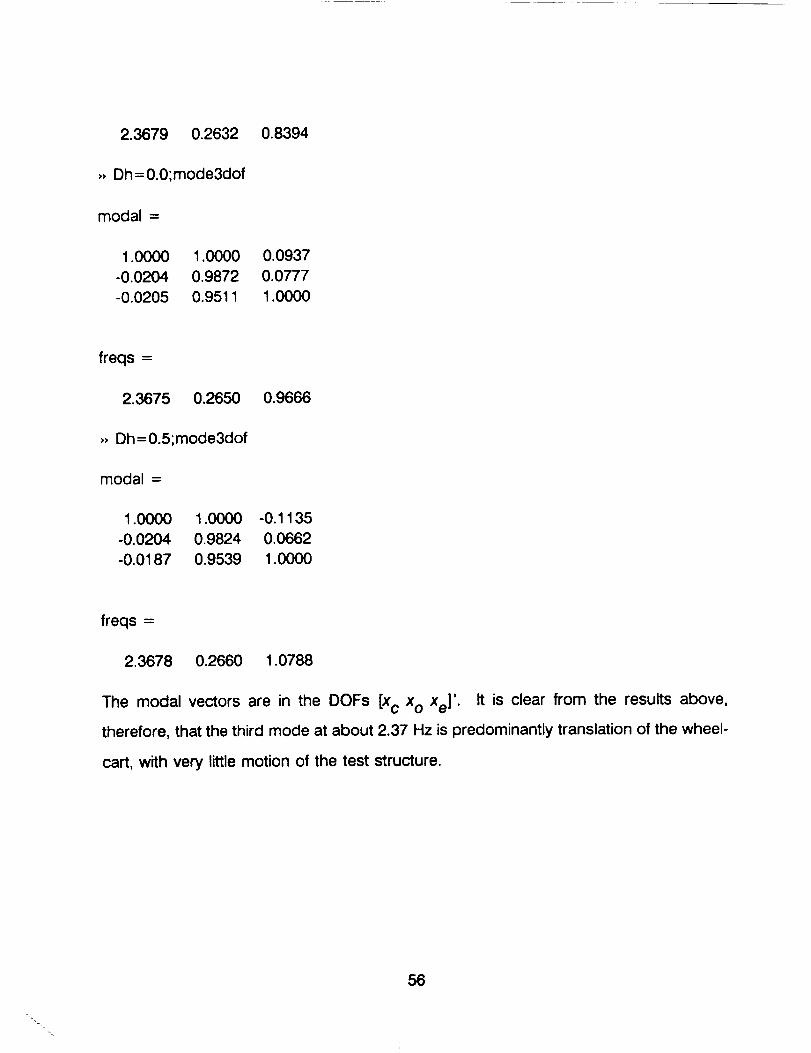
2.3679 0.2632
,, Dh=0.0;mode3dof
modal =
0.8394
1.0000 1.0000 0.0937
-0.0204 0.9872 0.0777
-0.0205 0.9511 1.0000
freqs --
2.3675 0.2650
,, Dh=0.5;mode3dof
modal =
0.9666
1.0000 1.0000 -0.1135
-0.0204 0.9824 0.0662
-0.0187 0.9539 1.0000
freqs =
2.3678 0.2660 1.0788
The modal vectors are in the DOFs [x c x o Xe]'. It is clear from the results above,
therefore, that the third mode at about 2.37 Hz is predominantly translation of the wheel-
cart, with very little motion of the test structure.
56
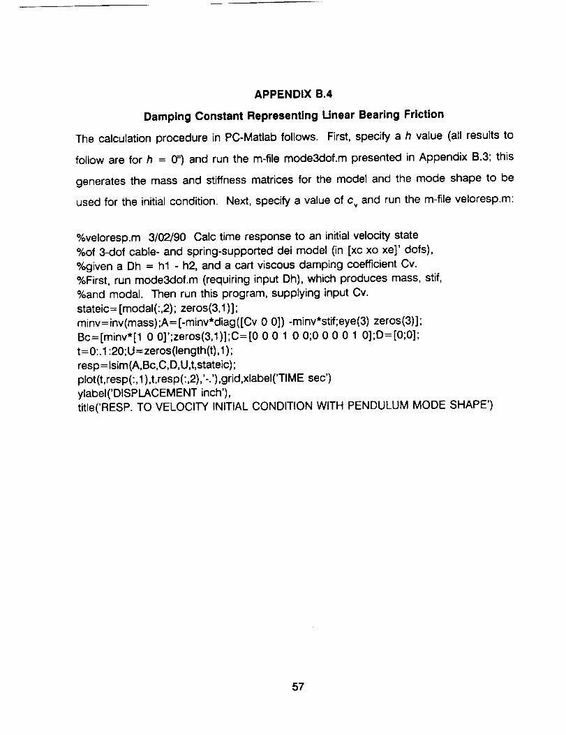
APPENDIX B.4
Damping Constant Representing Linear Bearing Friction
The calculation procedure in PC-Matlab follows. First, specify a h value (all results to
follow are for h = 0") and run the m-file mode3dof.m presented in Appendix B.3; this
generates the mass and stiffness matrices for the model and the mode shape to be
used for the initial condition. Next, specify a value of c v and run the m-file veloresp.m:
%veloresp.m 3/02/90 Calc time response to an initial velocity state
%of 3-dof cable- and spring-supported dei model (in [xc xo xe]' dofs),
%given a Dh = hl - h2, and a cart viscous damping coefficient Cv.
%First, run mode3dof.m (requiring input Dh), which produces mass, stif,
%and modal. Then run this program, supplying input Cv.
stateic = [modal(:,2); zeros(3,1 )];
minv =inv(mass);A= [-minv*diag([Cv 0 0]) -minv*stif;eye(3) zeros(3)];
Bc=[minv*[1 0 0]';zeros(3,1)];C=[0 0 0 1 0 0;0 0 0 0 1 0];D=[0;0];
t =0:.1:20;U = zeros(length(t), 1);
resp = Isim (A, Bc, C, D, U,t, stateic);
plot (t,resp(:, 1),t,resp(:,2),'-.'),grid,xlabel('TIME sec')
ylabeI('DISPLACEMENT inch'),
title('RESP. TO VELOCITY INITIAL CONDITION WITH PENDULUM MODE SHAPE')
57

APPENDIX B.5
Proportional Control
%statmats.m rood 1 3/04/90 Calc state matrices of 3-dof cable- and
%spring-supported dei model (in [xc xo xe]' dofs), given a Dh = hl - h2,
%Cv = the viscous damping coefficient of the cart bearing,
%and dob = the ratio d/b. Required inputs are Dh, Cv and dob.
%The matrices calculated are the 3x3 mass, minv, and stif, and
% A = the 6x6 plant state matrix,
% Bc = the 6xl control input matrix,
% Bd = the 6xl disturbance input matrix for excitation fe,
% C = the lx6 output matrix for measuring xe,
% D = [0],
% Ceps = the lx6 output matrix for eps = xd - xc.
Mg = 99.48;g = 386.4; M = Mg/g; Mw = 2/g; Iw= 338/g;I = 1777/g;It = I+ Iw;mi = 1/M;
b = 3; L = 88.625; Kx = .756; Kt = 194.5; Dhb = Dh + b;m3 = IUb ^ 2; Kg = M'g/L; RDh = Dh/b;
RDhb = RDh + 1 ;kl = Kg*RDhb; k2= Kg*RDh;k3= Kt/b ^ 2;k4=-(k3+ k2* (L/b + RDhb));
mass=[Mw 0 0;0 M+m3 -m3;0 -m3 m3];minv=[1/Mw 0 0;0 mi mi;0 mi mi+l/m3];
stir= [Kg -kl k2;-kl k3+Kg*(RDhb ^ 2+RDh*L/b) k4;k2 k4 Kx+k3+k2*(L,/b+RDh)];
A=[-minv*diag([Cv 0 0]) -minv*stif;eye(3) zeros(3)];
Bc= [minv*[1 0 0]';zeros(3,1 )];Bd= [minv*[0 0 1]';zeros(3,1)];
C=[0 0 0 0 0 1];D=[0];Ceps=[0 0 0 -1 dob 1-dob];
The eigenvalues and eigenvectors of _ reflect the character of the closed-loop
system, Eq. 27. The procedure for calculating relevant parts of the eigensolution with
PC-Matlab follows. First, specify values for h, c v and d/b. The eigenvalues and
eigenvectors of A¢ vary with feedback constant Cp. Hence, next specify an array of
Cp values with the statement "Cp=lst value:increment:last value" (supply numerical
values for 1st value, etc.), or with a "logspace" statement if an array equally spaced on
the logarithmic scale is desired. Then run m-file proprloc.m:
%proprloc.m (04 Apr 90): Proportional control of horizontal motion;
%program plots locus of damped freqs vs. zetas of translation mode of
%3-DOF model as proportional feedback constant Cp varies;
%Action req'd to execute:
% First enter values for Dh, Cv and dob;
% next enter 'Cp=lst value:increment:last value;proprloc',
58
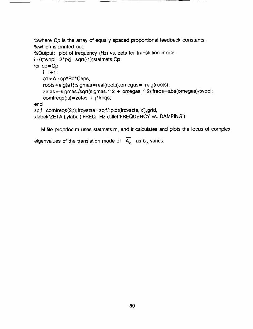
%where Cp is the array of equally spaced proportional feedback constants,
%which is printed out.
%Output: plot of frequency (Hz) vs. zeta for translation mode.
i= 0;twopi=2*pi;j =sqrt(- 1);statmats;Cp
for cp=Cp;
i=i+l;
al =A+cp*Bc*Ceps;
roots = eig (a 1);sigmas = real (roots);omegas = imag (roots);
zetas =-sigmas./sqrt(sigmas. ^ 2 + omegas. ^ 2);freqs = abs(omegas)/twopi;
comfreqs(:,i)=zetas + j*freqs;end
zpjf=comfreqs(3,:);frqvszta=zpjf.';plot(frqvszta,'x'),grid,
xlabel('ZETA'),ylabel('FREQ Hz'),title('FREQUENCY vs. DAMPING')
M-file proprloc.m uses statmats.m, and it calculates and plots the locus of complex
eigenvalues of the translation mode of _ as Cp varies.
59
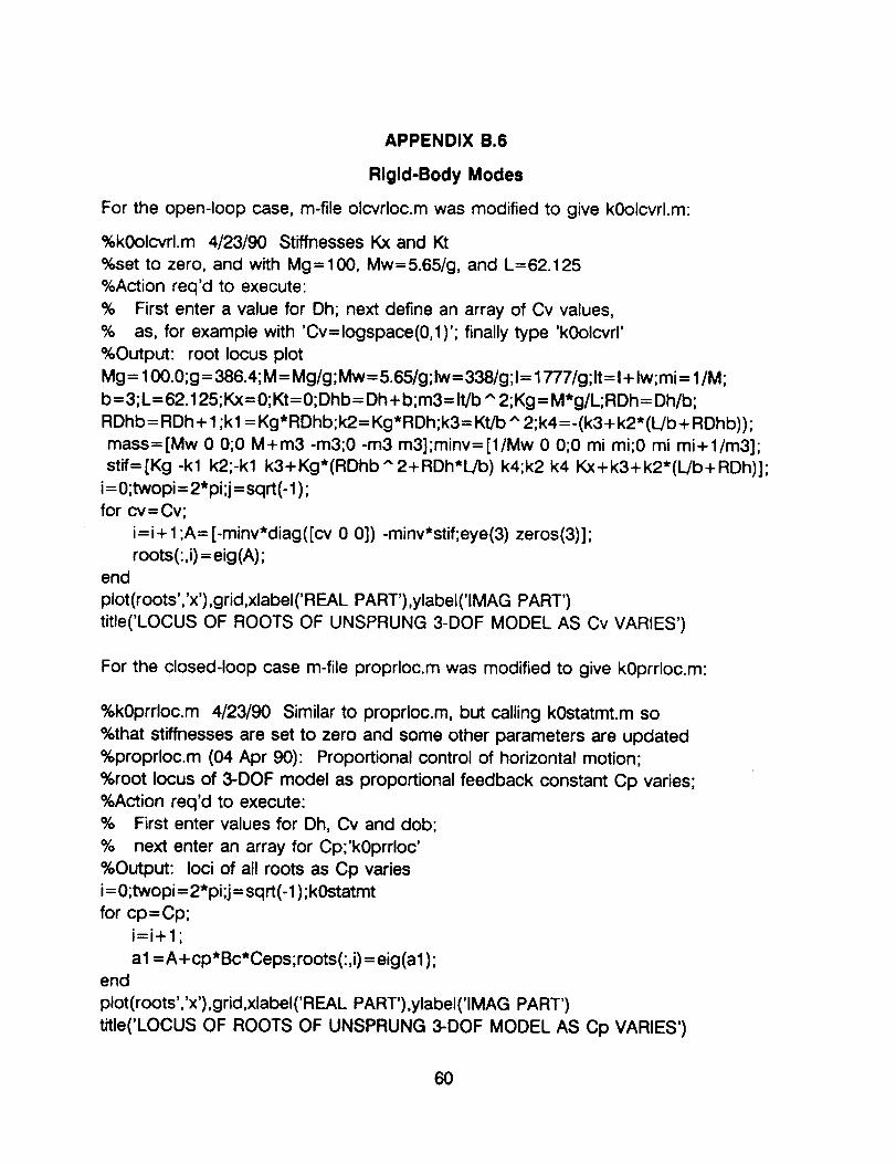
APPENDIX B.6
Rigid-Body Modes
For the open-loop case, m-file olcvrloc.m was modified to give k0olcvrl.m:
%k0olcvrl.m 4/23/90 Stiffnesses Kx and Kt
%set to zero, and with Mg=100, Mw=5.65/g, and L=62.125
%Action req'd to execute:
% First enter a value for Dh; next define an array of Cv values,
% as, for example with 'Cv=logspace(0,1)'; finally type 'k0olcvrl'
%Output: root locus plot
Mg= 100.0;g = 386.4; M = Mg/g;Mw= 5.65/g;Iw= 338/g;I = 1777/g;It= I + Iw;mi = l/M;
b=3; L=62.125; Kx= 0;Kt=0;Dhb= Dh + b;m3= ItJb ^ 2;Kg= M'g/L; RDh = DhPo;
RDhb= RDh + 1 ;k 1= Kg*RDhb;k2 = Kg*RDh;k3= Kt/b ^ 2; k4 =-(k3+ k2* (L/b + RDhb));
mass=[Mw 0 0;0 M+m3 -m3;0 -m3 m3];minv--[1/Mw 0 0;0 mi mi;0 mi mi+ 1/m3];
stif=[Kg-kl k2.;-kl k3+Kg*(RDhb^2+RDh*lJb)k4;k2 k4 Kx+k3+k2*(L/b+RDh)];
i=0;twopi=2*pi;j=sqrt(-1 );
for cv=Cv;
i=i+l ;A= [-minv*diag([cv 0 0]) -minv*stif;eye(3) zeros(3)];
roots(:,i) =eig(A);
end
piot(roots','x'),grid,xlabel('REAL PART'),ylabeI('IMAG PART')
title('LOCUS OF ROOTS OF UNSPRUNG 3-DOF MODEL AS Cv VARIES')
For the closed-loop case m-file proprloc.m was modified to give k0prrloc.m:
%k0prrloc.m 4/23/90 Similar to proprloc.m, but calling k0statmt.m so
%that stiffnesses are set to zero and some other parameters are updated
%proprloc.m (04 Apr 90): Proportional control of horizontal motion;
%root locus of 3-DOF model as proportional feedback constant Cp varies;
%Action req'd to execute:
% First enter values for Dh, Cv and dob;
% next enter an array for Cp;'k0prrloc'
%Output: loci of all roots as Cp varies
i = 0;twopi = 2*pi;j = sqrt(- 1); k0statmt
for cp=Cp;
i=i+l;
al =A+cp*Bc*Ceps;roots(:,i)=eig(al);end
plot(roots','x'),grid,xlabel('REAL PART'),ylabeI('IMAG PART')
title('LOCUS OF ROOTS OF UNSPRUNG 3-DOF MODEL AS Cp VARIES')
6O

M-file kOstatmt.m referred to in kOprrloc.m is the same as statmatsom, except that the
values for k,,, k e, mg, m,,g and Qwere changed as stated above. Results of kOprrloc.m
are recorded on Figures 27 a-c.
61

APPENDIX B.7
PID CONTROL
Given a single value for each of the PID coefficients, pidroots.m listed below calculates
all of the roots:
%pidroots.m 22 Apr 1990
%enter Dh, then run mode3dof.m, then run dobcalc.m to calc dob
%Enter Cv; then run statmats.m to calc A, Bc and Ceps%Enter taud; prog. calcs Az and Bz
%Specify Cp and Ci and Cd;prog. calls freqzeta to calc roots
itaud = 1/taud;Az= [0 0;0 -itaud] ;Bz = [1 ;itaud] ;A21 = Bz*Ceps;
con = Cd/taud; Cz = [Ci -con] ;Dz = Cp + con;
a= [A+ Dz*Bc*Ceps Bc*Cz;A21 Az] ;freqzeta
Two m-files calculate the loci of translation mode roots of Eq. 33 as controller coefficients
vary. Program pidrlocd.m calculates the locus as C d varies, with Cp and Ci fixed:
%pidrlocd.m 27 Apr 1990 Calculates the freq-zeta locus of the transl.
%mode of the 3-DOF model as derivative coefficient Cd varies.
%enter Dh, then run mode3dof.m, then run dobcalc.m to calc dob
%Enter Cv; then run statmats.m to calc A, Bc and Ceps
%Enter taud; prog. calcs Az and Bz
%Specify Cp and Ci and an array of values for Cd.
itaud = 1/taud;Az= [0 0;0 -itaud] ;Bz= [1 ;itaud] ;A21 = Bz*Ceps;
i=0;j=sqrt(-1 );twopi=2*pi;Cdfor cd=Cd
i= i+ 1;con = cd/taud;Cz = [Ci -con] ;Dz = Cp +con;
a=[A+Dz*Bc*Ceps Bc*Cz;A21 Az];
,roots = eig (a);sigmas = real (roots);omegas = imag (roots);
zetas=-sigmas./sqrt(sigmas. ^ 2 + omegas. ^ 2);freqs=abs(omegas)/twopi;comfreqs(:,i)=zetas + j*freqs;
end
zpjf=comfreqs(6,:);frqvszta=zpjf.';plot(frqvszta,,x,),grid,
xlabeI('DAMPING FACTOR, ZETA'),ylabeI('DAMPED FREQ Hz'),
title('LOCUS OF FREQ-ZETA OF 3-DOF CL-PID MODEL AS Cd VARIES')
Similarly, pidrloci.m calculates the locus as Ci varies, with Cp and C d fixed:
62

%pidrloci.m 27 Apr 1990 Calculates the freq-zeta locus of the transl.
%mode of the 3-DOF model as integral coefficient Ci varies.
%enter Dh, then run mode3dof.m, then run dobcalc.m to calc dob
%Enter Cv; then run statmats.m to calc A, Bc and Ceps
%Enter taud; prog. calcs Az and Bz
%Specify Cp and Cd and an array of values for Ci.
itaud = 1/taud;Az= [0 0;0 -itaud];Bz= [1 ;itaud] ;A21 = Bz*Ceps;
i=0;j=sqrt(-1);twopi=2*pi;Cifor ci=Ci
i= i + 1 ;con = Cd/taud; Cz = [ci -con]; Dz = Cp + con;
a= [A+ Dz*Bc*Ceps Bc*Cz;A2.1 Az];
roots = eig (a) ;sig m as = real (roots) ;o meg as = imag (roots);
zetas =-sigmas./sqrt(sigmas. ^ 2 + omegas. ^ 2);freqs= abs(omegas)/twopi;
comfreqs(:,i)=zetas + j*freqs;end
zpjf=comfreqs(6,:);frqvszta=zpjf.';plot(frqvszta,'x'),grid,
xlabeI('DAMPING FACTOR, ZETA'),ylabeI('DAMPED FREQ Hz'),
title('LOCUS OF FREQ-ZETA OF 3-DOF CL-PID MODEL AS Ci VARIES')
To generate the results shown on Figure 28, each of the three m-files was run
separately, and its root locus was saved (with the "save" command in PC-Matlab). Then
all three loci were loaded together (with the "load" command in PC-Matlab) and plotted
on the same graph.
63
APPENDIX C
DIGITAL CONTROLLER PROGRAM
The control program implemented in the Spectrum Signal Processing TMS320C25
System Board is listed below. The program is written in TI (Texas Instruments) COFF
assembly language. The program is compiled and linked with the TI COFF Assembler
and Linker programs supplied with the system. To implement the executable program
in the system board it must be downloaded using the Spectrum MON25 monitor
program also supplied with the system.
**********************************'k _******
* Two Channel Sample *
* With output proportional to error ** TMS320C25 *
********_*********************************
* Author : R. Gold
* Dynamic Engineering, Inc.
* Tel (804) 873-1344
* Date 4/23/90
* 320C25 LINKS
* DEFINE ADDRESS CONSTANTS
VAL0: .equ 01 h
VALI: .equ 02h
AY0: .equ 03h
AY1 : .equ 04h
ERR: .equ 05h
TIMER: .equ 09h
STAT: .equ 08h
CTRL: .equ 08h
64
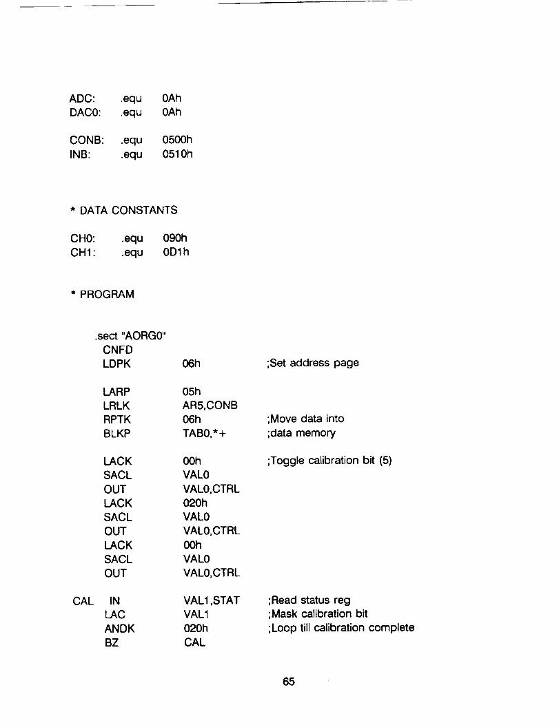
ADC: .equ 0Ah
DAC0: .equ 0Ah
CONB: .equ 0500h
INB: .equ 051 Oh
* DATA CONSTANTS
CH0: .equ 090h
CH1 : .equ 0Dlh
* PROGRAM
.sect "AORG0"
CNFD
LDPK
LARP
LRLK
RPTK
BLKP
LACK
SACL
OUT
LACK
SACL
OUT
LACK
SACL
OUT
CAL IN
LAC
ANDK
BZ
06h
05h
AR5,CONB
06h
TAB0,* +
00h
VAL0
VAL0,CTRL
020h
VAL0
VAL0,CTRL
00h
VAL0
VAL0,CTRL
VAL1 ,STATVAL1
020h
CAL
;Set address page
;Move data into
;data memory
;Toggle calibration bit (5)
;Read status reg
;Mask calibration bit
;Loop till calibration complete
65
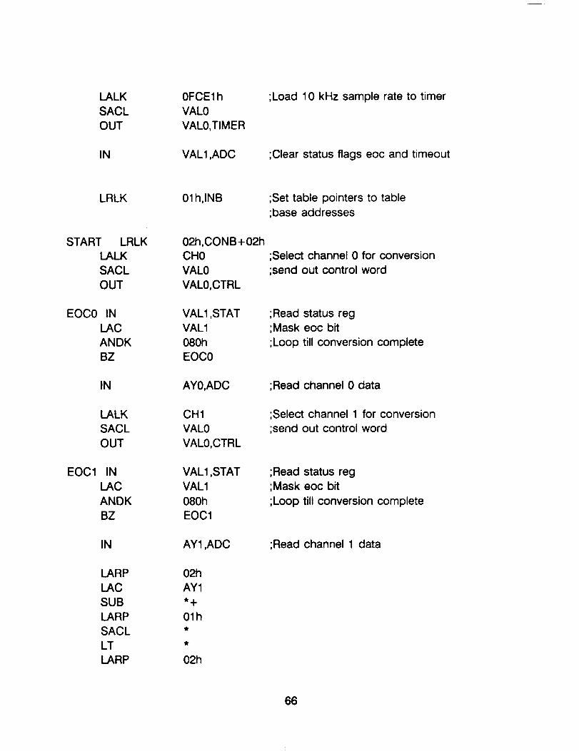
LALK
SACL
OUT
0FCE1 h
VAL0
VAL0,TIMER
;Load 10 kHz sample rate to timer
IN VAL1 ,ADC ;Clear status flags eoc and timeout
LRLK 01 h,INB ;Set table pointers to table
;base addresses
START LRLK
LALK
SACL
OUT
02h,CONB+02h
CH0
VAL0
VAL0,CTRL
;Select channel 0 for conversion
;send out control word
EOC0 IN
LAC
ANDK
BZ
VAL1 ,STATVAL1
080h
EOC0
;Read status reg;Mask eoc bit
;Loop till conversion complete
IN AY0,ADC ;Read channel 0 data
LALK
SACL
OUT
CH1
VAL0
VAL0,CTRL
;Select channel 1 for conversion
;send out control word
EOC1 IN
LAC
ANDK
BZ
VAL1 ,STAT
VAL1
080h
EOC1
;Read status reg;Mask eoc bit
;Loop till conversion complete
IN AY1 ,ADC ;Read channel 1 data
LARP
LAC
SUB
LARP
SACL
LT
LARP
02h
AY1
*+
01h
02h
66
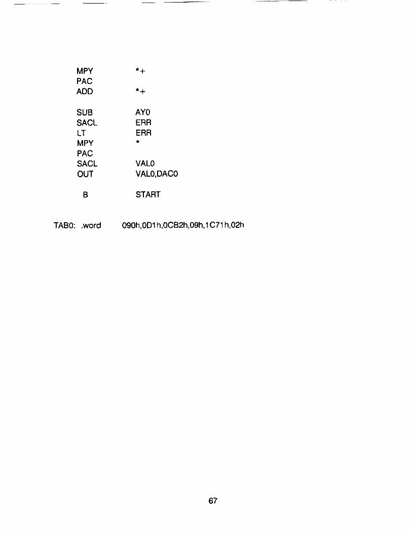
MPY
PAC
ADD
SUB
SACL
LT
MPY
PAC
SACL
OUT
AY0
ERR
ERR_t
VAL0
VAL0,DAC0
B START
TAB0: .word 090h,0D 1 h,0CB2h,09h, 1C71 h,02h
67
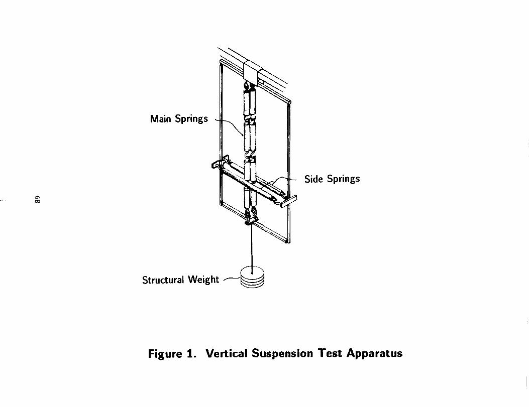
O_
GO
Main Springs ,.
Side Springs
Structural Weight _--"_ _
Figure 1. Vertical Suspension Test Apparatus
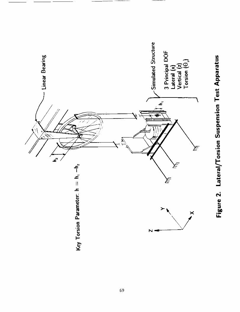
el
N_
Ill
llgem
l..i_
69
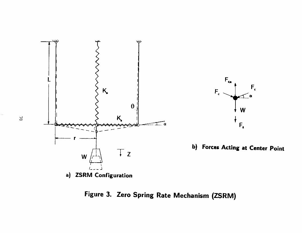
0
L
K,
0
a) ZSRM Configuration
Fc _ c
F,,
b) Forces Acting at Center Point
Figure 3. Zero Spring Rate Mechanism (ZSRM)
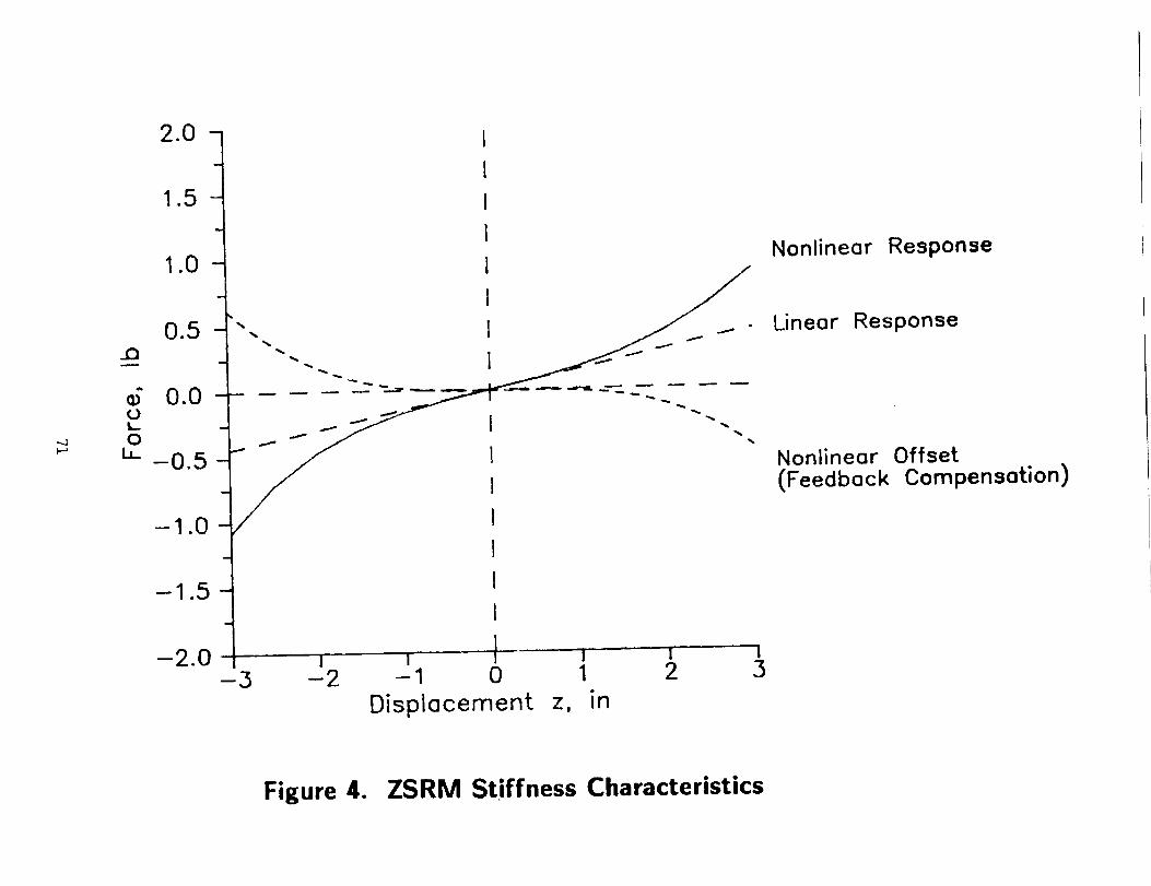
2.0
-.J
1.0
-1.0
-1.5
Nonlinear
Linear
Nonlinear(Feedback
Response
Response
OffsetCompensation)
-3
1i t - t l I i
-2 -1 0 1 2 3
Displocement z, in
Figure 4. ZSRM Stiffness Characteristics

1.0
(d m
m
o
Km
0.8
0.6
60/0 0
0.4
Pcrit
Km
2
F
0.2
0.0 I0.0 0.2 0.4 0.6 0.8 I .0
Pc/Pcrit
Figure 5. Effect of Side Spring Preload on System Frequency
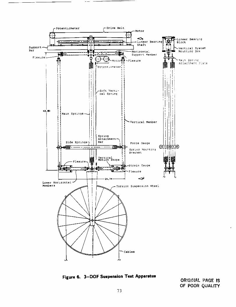
Potentiometer
SupportBar
r----Flexure
q
Belt
-Soft Verti-
cal Spring
43.
Main Springs----.-
Shaft
Support Member
_Vertical Member
Side Springs-
SpringAt
Force Gauge
Soring Mounting
Bracket
Lower Horizontal
Members
;train Gauge
Flexure
rsion Suspenszon Wheel
Lznear Bearlng
lock
Vertzcal System
Mounting Box
Mazn $prznq
Attachment _[ate
Cables
Figure 6. 3-DOF Suspension Test Apparatus
73
OR{G!NAL PAGE IS
OF POOR QUALITY
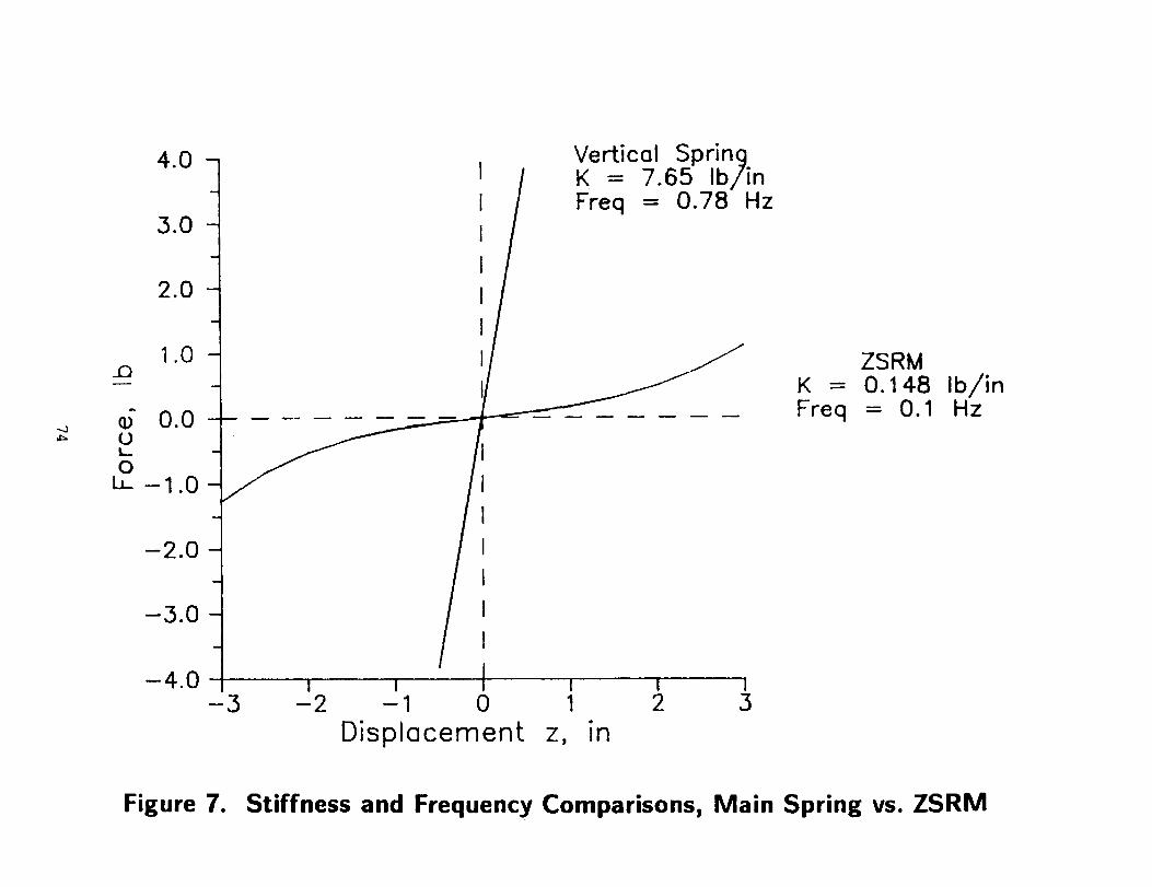
4.0
3.0
2.0
1.0_Q
-1.0
-2.0
Vertical Spring= 7.65 Ib/inFreq = 0.78
I I1 I I-3 -2 -1 0 1 2 3
Displecement z, in
Hz
ZSRMK = 0,148 Ib/inFreq = 0.1 Hz
Figure 7. Stiffness and Frequency Comparisons, Main Spring vs. ZSRM
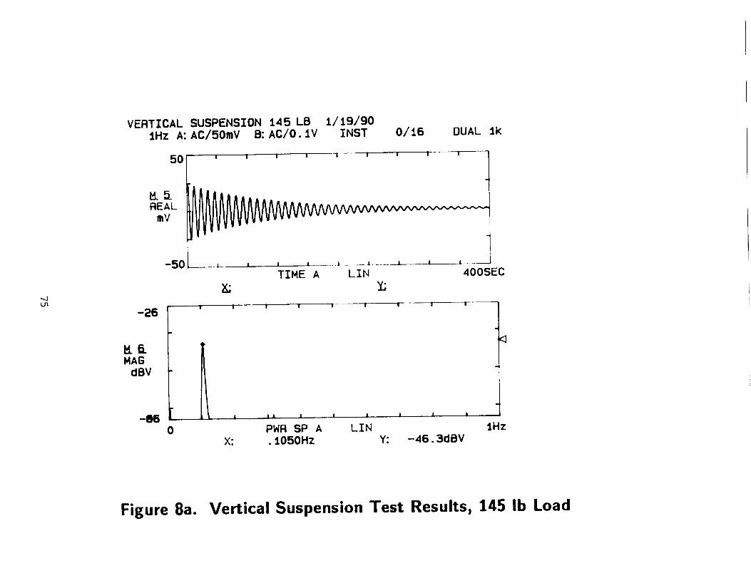
_J_n
VERTICAL SUSPENSION 145 LBIHz A:AC/5OmV B:AC/O.1V
I i /
50 l
_.5REAL
mV
-5O
-26
M6MAG
dBV
1/19/90INST O/CB DUAL lk
I i i I i i
__J._ I i l .... l _ .L ..... I I 1
TIME A LIN 400SEC
x: Y.;
i I i I- I _ " I i-'--
i I IL I, i i | I •
PWR SPA LIN
X: . t050Hz Y: -46.3dBV
IHz
Figure 8a. Vertical Suspension Test Results, 145 Ib Load
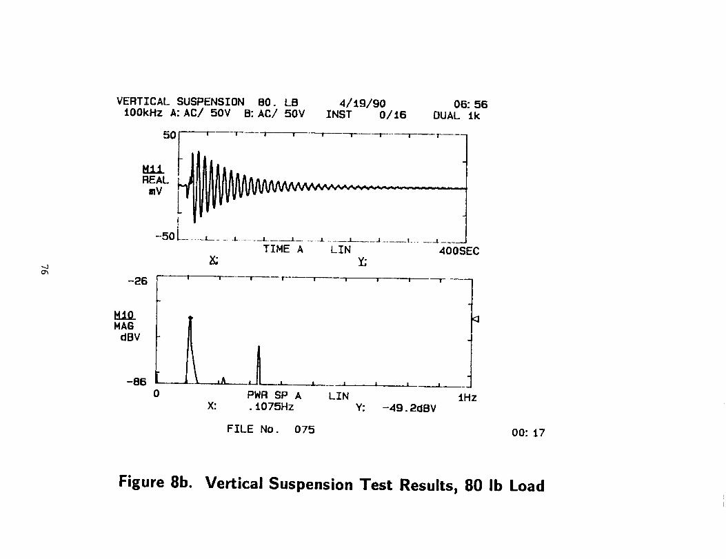
..jO_
VERTICAL SUSPENSION 80. LBtOOkHz A: AC/ 50V B: AC/ 50V
4/19/90 06:56INST 0/t6 DUAL tk
Y:
BiO_NAG
dBV
-86 _ , ., , .. _
0 1Hz
,_ LI , i . ,
PWR SPA LIN
X: .1075Hz
FILE No. 075
Y: -49.2dBV
00:17
Figure 8b. Vertical Suspension Test Results, 80 Ib Load
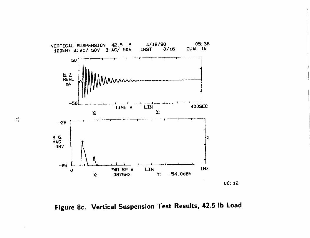
_J..J
VERTICAL SUSPENSION A2 5 LBtOOkHz A:AC/ 50V B:AC/ 50V
50_ r,_--1_-- ----lr r
4/t9/90 05:38INST 0/16 DUAL tk
T l-_ --I-- -"----"Ir_ --T
H. 7_REAL
mV
TIME A LIN
x: _C
-50 .... ,
-26 r_r--'t1
ME
dBV
-86 - '0
T ! r-------w
X:
i
4
L -- - L .... -_
400SEC
I4
I I I __ I I.... I
PWR SPA LIN.0875Hz Y: -54. OclBV
IHz
00:t2
Figure 8c. Vertical Suspension Test Results, 42.5 Ib Load
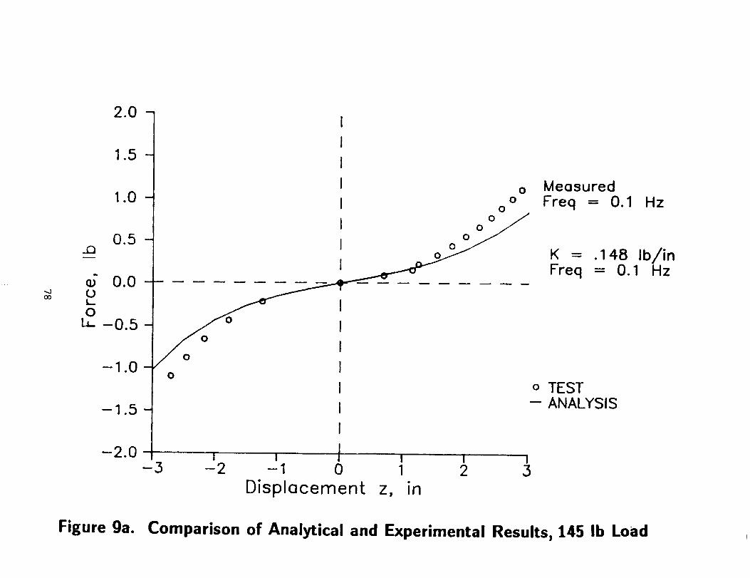
2.0 --
(3O
1.5 -
1.0
0.5
°_ 0.0
u_ -0.5
-1.0
-I .5 -
°o Measured
o° Freq = 0.1 Hzo
o o K = .148 IbFreq = 0.1 H/izn
0
-2.0 I I ! I I I
-3 -2 -1 0 1 2 3
Displacement z, in
o TEST-- ANALYSIS
Figure 9a. Comparison of Analytical and Experimental Results, 145 Ib Load
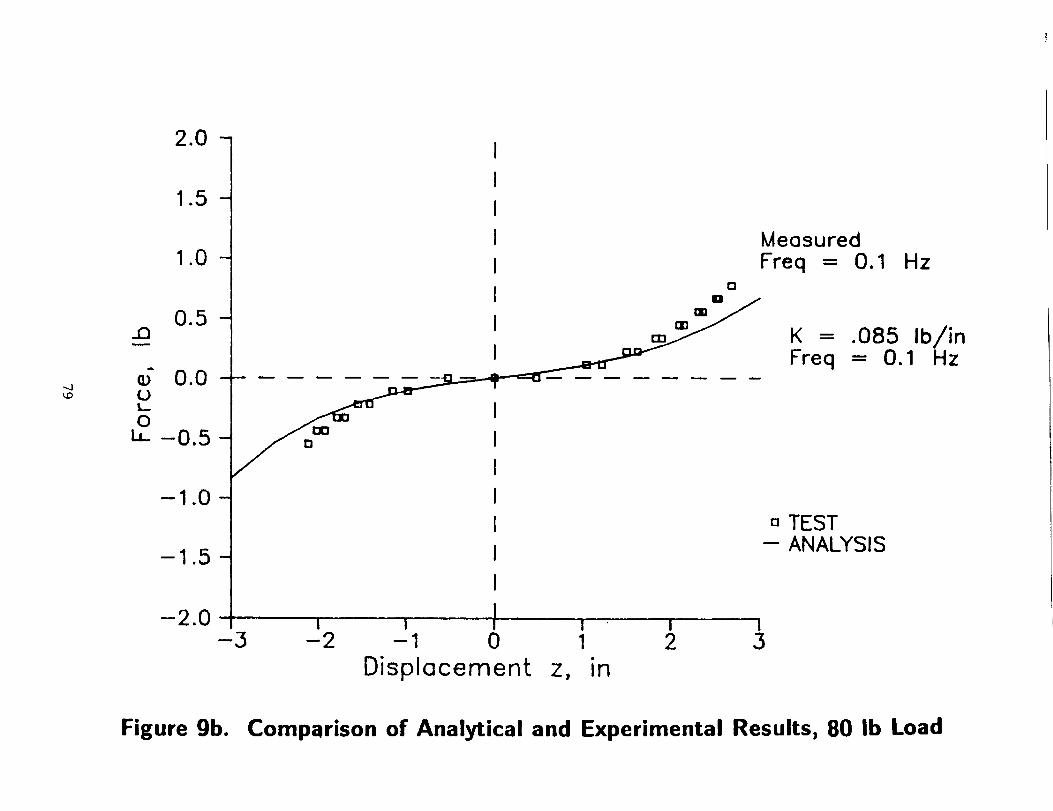
2.0 -
-..J
1,5 -
1.0
0.5
0.0
u_ -0.5
-1.0 -
-1.5 -
Meosured
a Freq = 0.1 Hz
__ K = .085 Ib/inFreq - 0.1 Hz
-2.0, _ _ i i i-3 -2 -1 0 1 2 3
Displacement z, in
a TEST-- ANALYSIS
Figure 9b. Comparison of Analytical and Experimental Results, 80 Ib Load
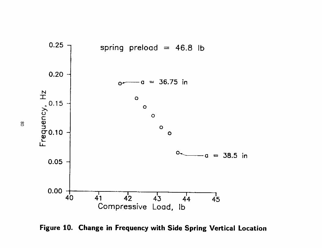
Go0
Nt
0.25
0.20 -
t,...LL
0.05
0.00
spring preload = 46.8 Ib
o.*------a = 36.75 in
0
0
0
0
0
o.,._ a = 38.5 in
,=,,, , , i
I i i i i40 41 42 43 44 45
Compressive Load, Ib
Figure 10. Change in Frequency with Side Spring Vertical Location
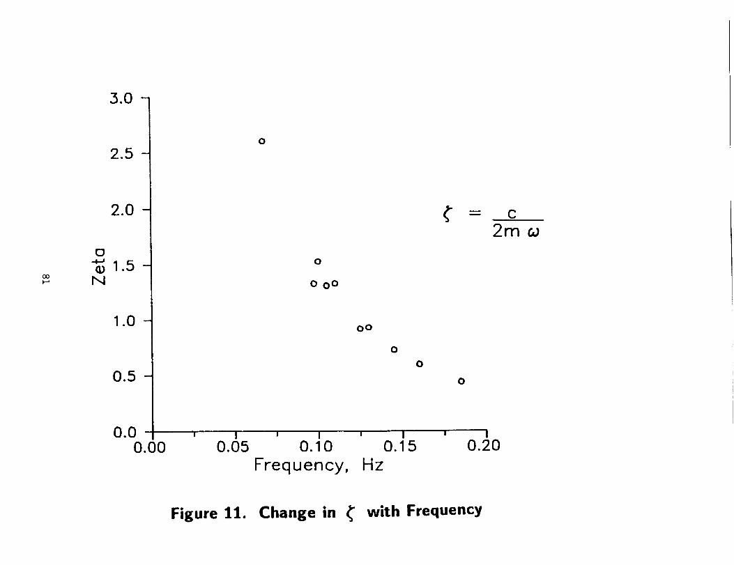
3.0 --
(30
o
N
2.5 --
2.0 --
1.5 -
1.0 --
0.5 -
0.00.00
0
0
0 0 o
O0
0
0
0
I ' I ' I ' i
0.05 0.10 0.15 0.20
Frequency, Hz
C
2m co
Figure 11. Change in _ with Frequency
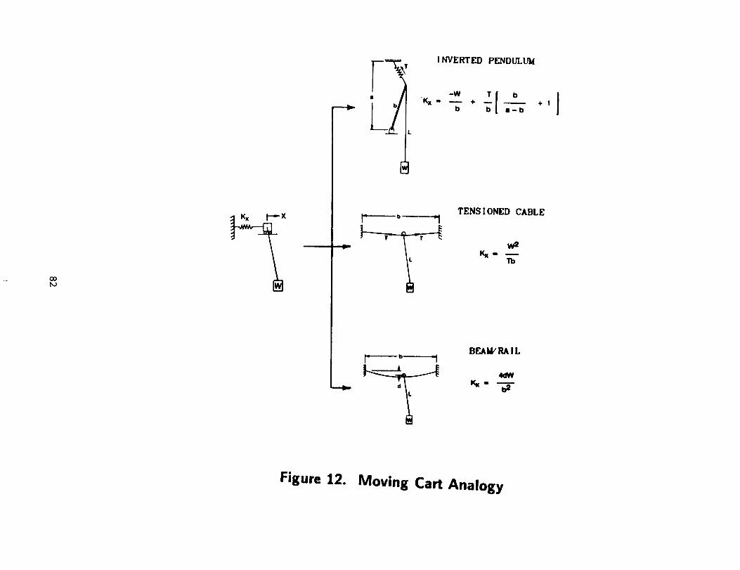
oo
INYERTED PENDULUM
_w ,io I'Kx " _ + + 1b b a-t)
TENSIONED CABLE
Kx I i
BEAM/RAIL
Figure 12. Moving Cart Analogy
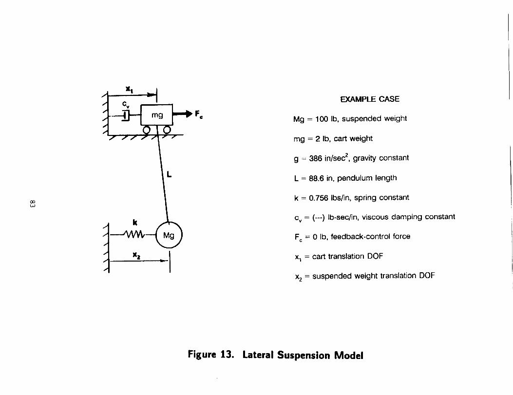
ooL_
XI
¥
F¢
/
/
/
/
/
X2
EXAMPLE CASE
Mg = 100 Ib, suspended weight
mg = 2 Ib, cart weight
g = 386 in/sec z, gravity constant
L = 88.6 in, pendulum length
k = 0.756 Ibs/in, spring constant
cv = (---) Ib-sec/in, viscous damping constant
Fc = 0 Ib, feedback-control force
x1 = cart translation DOF
xz = suspended weight translation DOF
Figure 13. Lateral Suspension Model
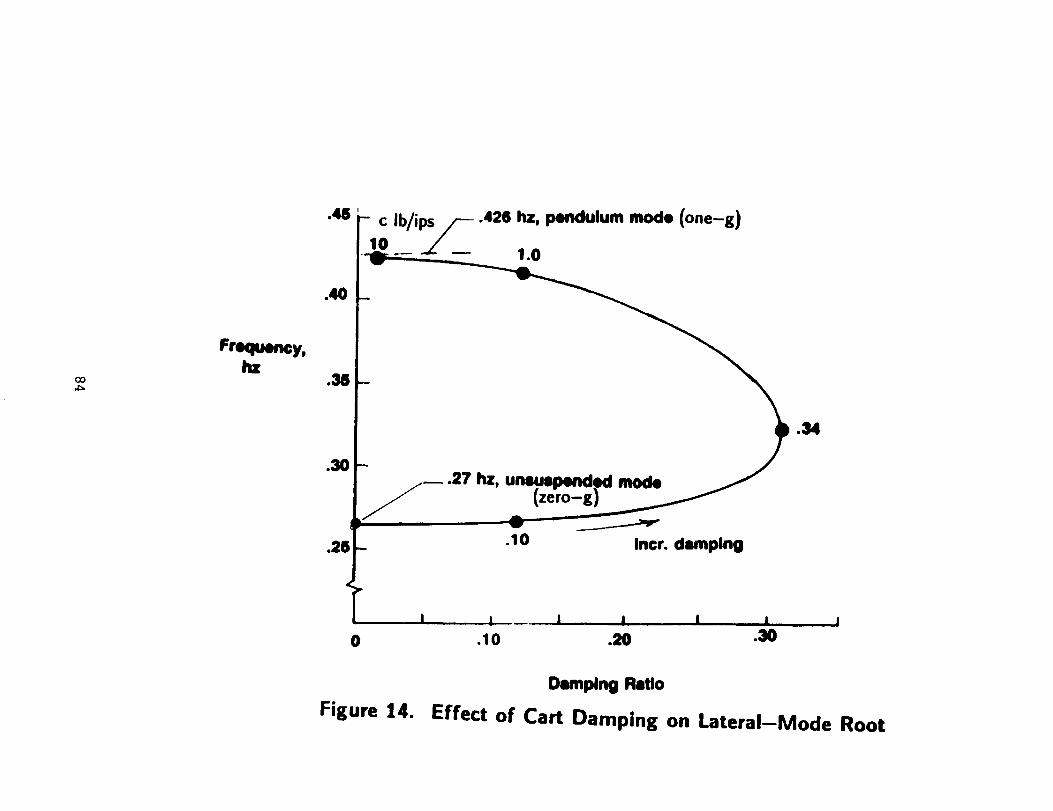
CO
.48
.40
Fre_ency,.38
.30
.28
0
- c Ib/i_ .426 hz, pendulum mode (one-g)2_ -- 1.o
_ .10 Incr. damping
I I I I l I ,
.10 .20 .30I
Figure 14.
Damping Ratio
Effect of Cart Damping on Lateral-Mode Root
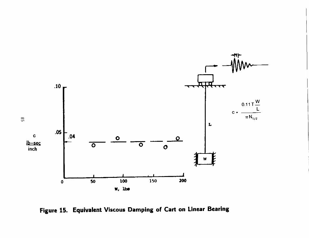
.10 -
-'_rt--
U1
C
inch
.O5 t
.04 o _.__ 90 0 0
l i 1, JI , , |
0 5O I00 150 200
W, lls
L
C i
0.11T wL
Figure 15. Equivalent Viscous Damping of Cart on Linear Bearing
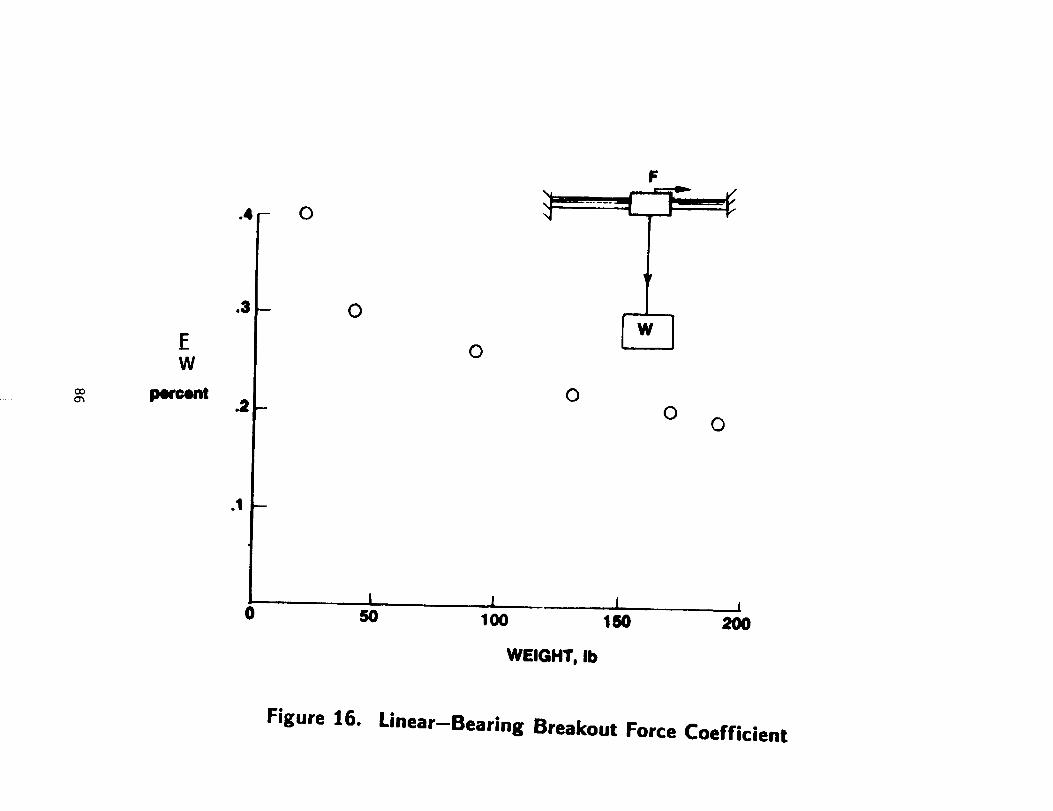
.4- O
F
COO_
EW
percent
.3
.2
.1
0
- 0
0
0
50 100 150 200
WEIGHT, Ib
Figure 16. Linear-Bearing Breakout Force Coefficient
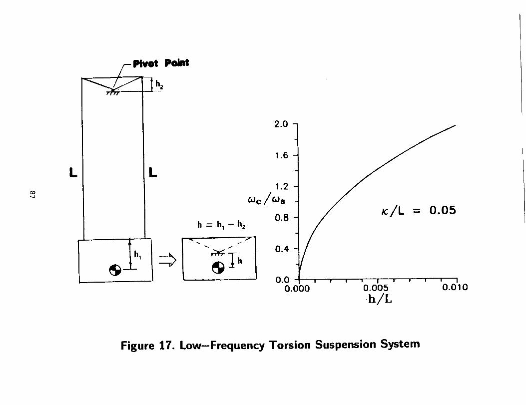
Pivot Point
O3-_J
L
Figure 17. Low-Frequency Torsion Suspension System
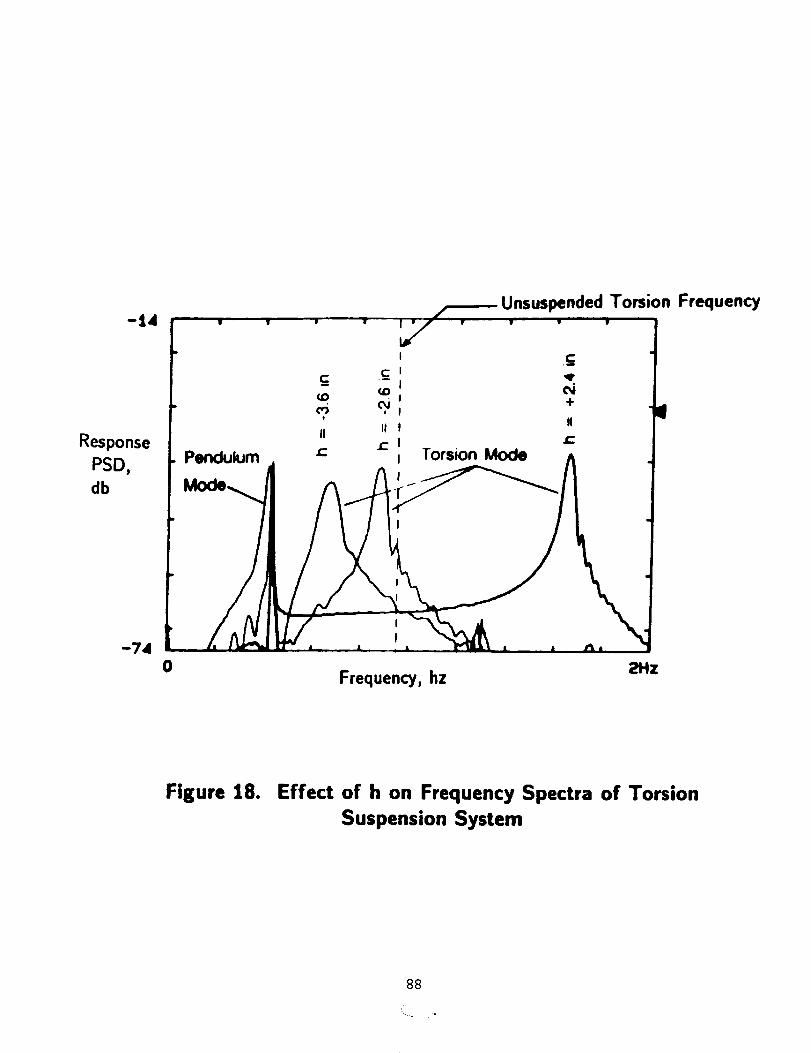
Unsuspended Torsion Frequency
-'4''" " "'_'" " "c"
c c_ _r- <o c_i
• _ _ + iiII II II
Response ; z: z:PSD, I. Pendulum , '- Torsion Mode h J
db
-74
0 Frequency, hz EHz
Figure 18. Effect of h on Frequency Spectra of Torsion
Suspension System
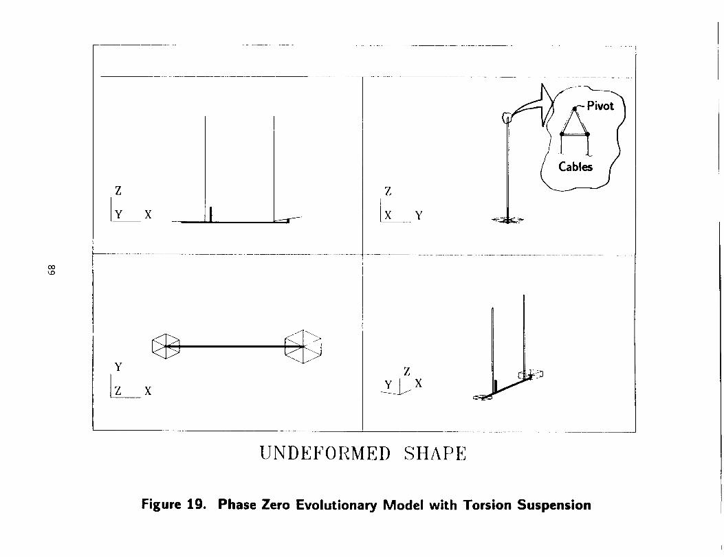
CO_0
Z
Y
X
X
Z
Y
li
ItH
UNDEFORMED SHAPE
Figure 19. Phase Zero Evolutionary Model with Torsion Suspension
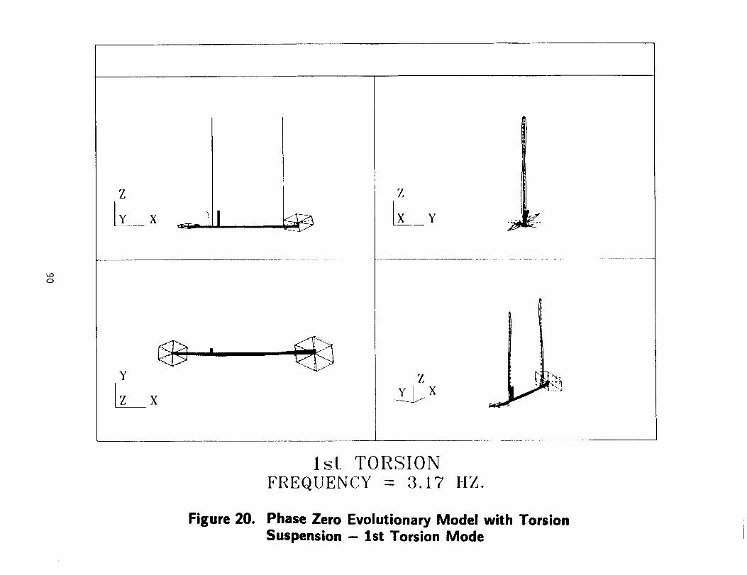
_OO
Z
X
X
Z
Y
Z
1 sL TORSION
FREQUENCY - 3.17 HZ.
Figure 20. Phase Zero Evolutionary Model with Torsion
Suspension - 1st Torsion Mode
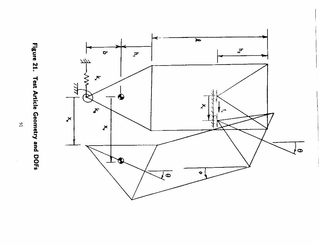
kO
i
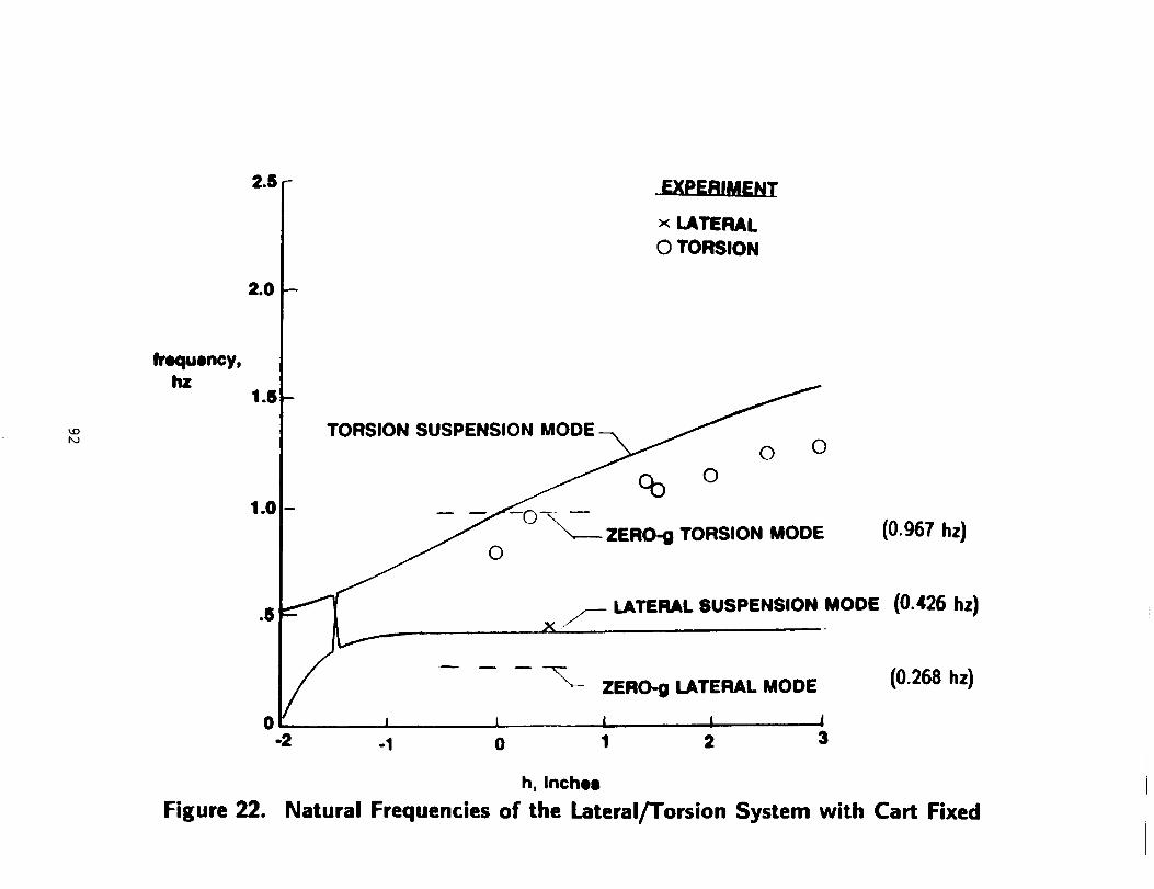
EXPERIMENT
x LATERAL
O TORSION
_O
frequency,hz
1.0
TORSION SUSPENSION MODE
O
O O
% o
ZERO-g TORSION MODE (0.967 hz)
jr- LATERAL SUSPENSION MODE (0.426 hz)
-1 0 1
h, Inchee
ZERO-g LATERAL MODE (0.268 hz)
l 1 J2 3
Figure 22. Natural Frequencies of the Lateral/Torsion System with Cart Fixed
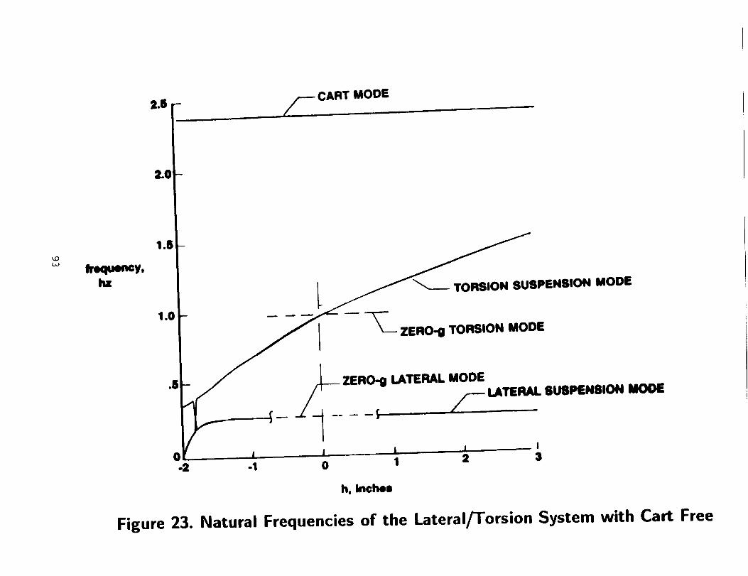
2.(
CART MODE
frequency,hz TORSION SUSPENSION MODE
-_ ZERO-g TORSION MODE
_ ZERO-g LATERAL MODE
_ _ _ f LATERAL 8USPEN$10N MODE
h, Inches
Figure 23. Natural Frequencies of the Lateral/Torsion System with Cart Free
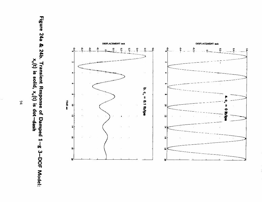
-rlme
OFCl
tD
O"
pI, _1
me _1
me
ox_
7c_O,,W
t_n_
IOCl
I
0"1"1
0
m
eo
I J--. I l I L _ I l
DISPLACaEMENT
i
OJ
!
t J
_._.___ ,o' ¸
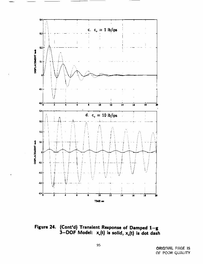
0,4
O,2
i 0
-GI
q _ v P
: ! c. _= llb/ips
1
- - L-_
_--4- ....
I,,i
4
i ' I
,,
6 | 10 12I i L
14 16 11
! ..... ; ...... __. ..... _:-
2D
]0
Figure 24. (Cont'd) Transient Response of Damped 1-g3-DOF Model: x_(t) is solid, Xo(t) is dot dash
95ORIG!NAL PAGE IS
OF POOR QUALITY
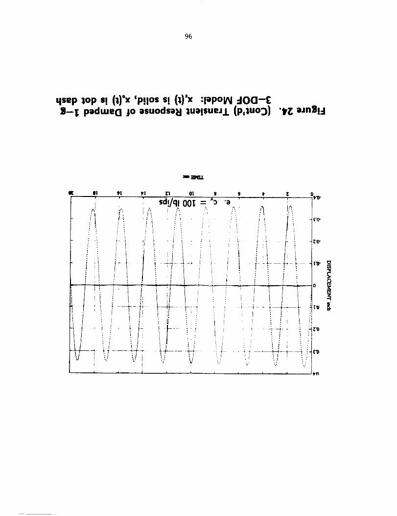
96
qsep :lop s! (:i)°x 'p!los s! (:l)='x :lapOlAI =lOQ-I_S-l[ padtueO jo asuodsaEI ;UalSUe,.L (p,luo:)) "t'Z:;_'nll!=l
I a]_lr.
!"
I i I i i i
Z'O-
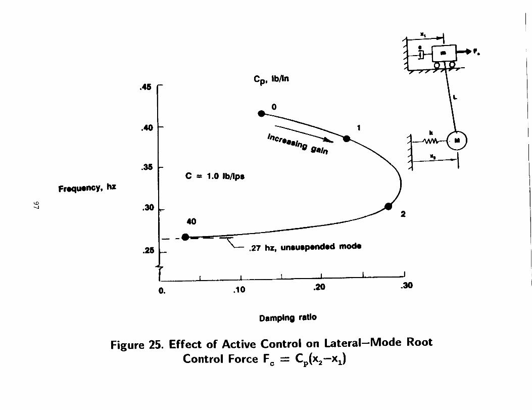
-.d
.45 -
o_ --
.25 _
Os
C = 1.0 Ib/Ips
4O
Cp, Ib/ln
2
_-- .27 hz, unsuspended mode
! I J [ I
.10 .20 .30
Damping ratio
Figure 25. Effect of Active Control on Lateral-Mode Root
Control Force Fc -- Cp(x2-xz)
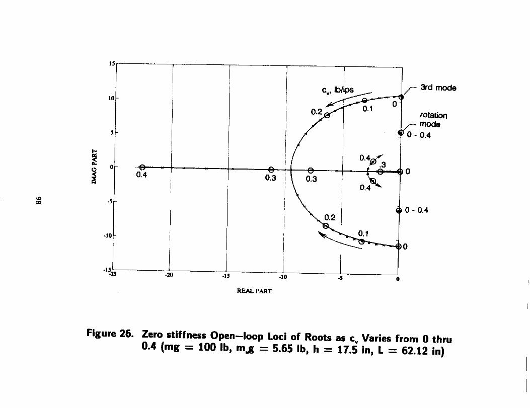
_OCO
15
10
-5
-10
-_5.z5J-20
7I
cv, Ib/ips
0
-I$ -I0 .$ 0
REAL PART
3rd mode
rotationmode
0 - 0.4
0
0 - 0.4
0
Figure 26. Zero stiffness Open-loop Loci of Roots as cv Varies from 0 thru
0.4 (rag = 100 Ib, m.g = 5.65 Ib, h = 17.5 in, L = 62.12 in)
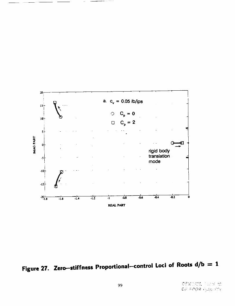
i=,
201 ,
E
51 ......
-5
{-151
"_..IL.8 .IL.6
a. C v
©
[]
= 0.05 Ib/ips
Cp = 0
Cp = 2
rigid bodytranslationmode
L *Jl t L_2_4
REAL PART
0
Figure 27. Zero-stiffness Proportional-control Loci of Roots d/b = 1
99
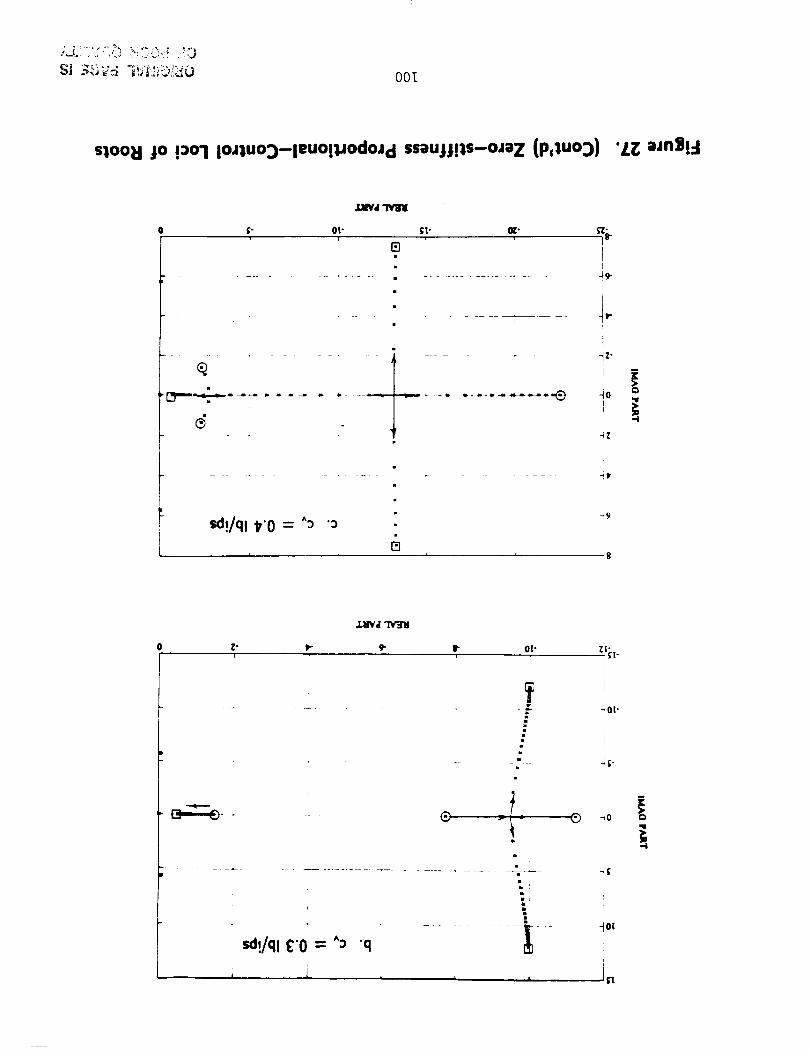
001
sloou jo !:)o3 Im;UO3-1euo!_odmd ss;)uJj!_s-m_Z (P,lUO3) "LZ:;unS!=l
J,_rd
f" Or" ;_- _- _.v
Io.
-,--............ -_ -io i-,4
i
4z
sd!/ql t"O = ^:)
L
":)_9
0 Z- _-! r
J.b'Vd
9" J-
sd!/ql £'0 = ^:) "q
i i i
- -- _01"
• i• ;
• _.
_ -_0
--- O[
i
fl
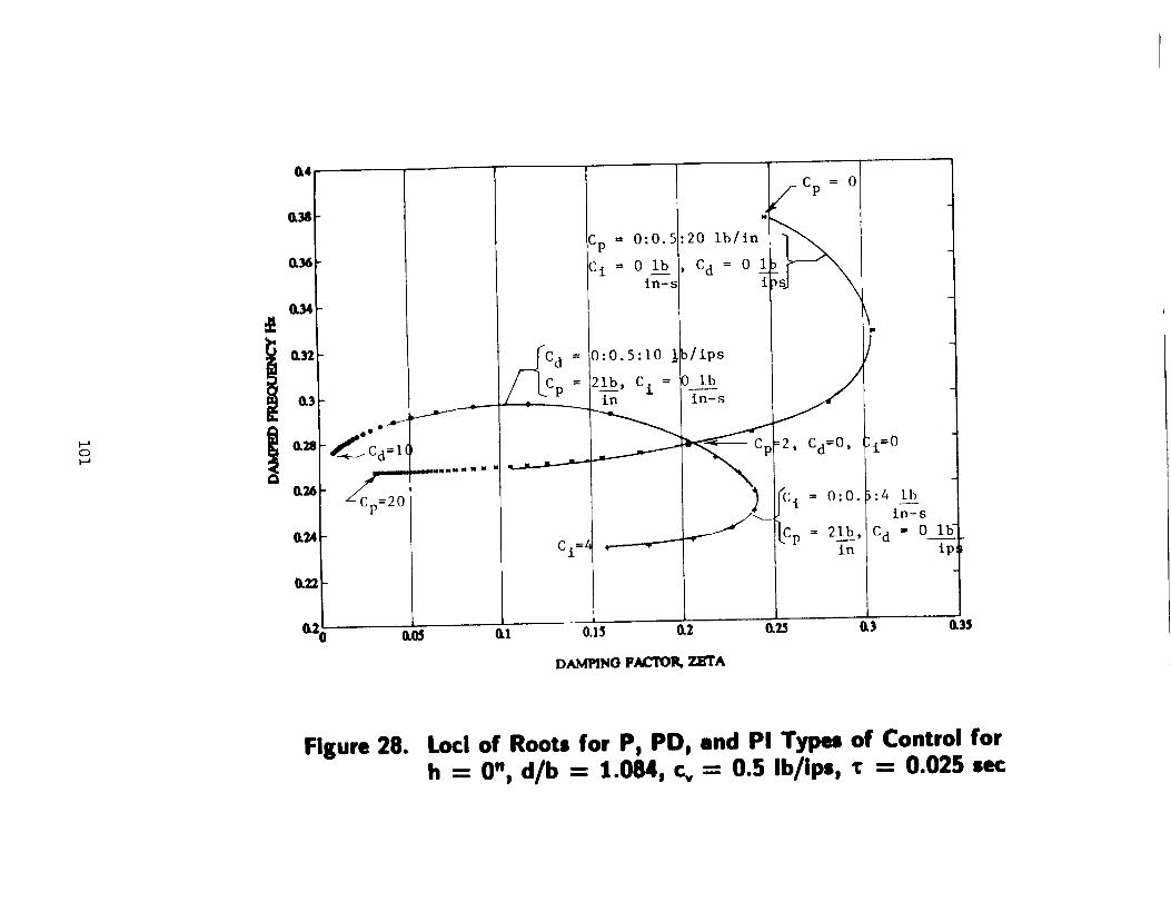
0
0.4
0,_
0.36
0.34
i 0.32O.3
O.26
0.24
O00_
_Cd=I
(k2o
_mmmm m N m
Cp = 0:0.
ci = o _bin-s
Cp= 0
:20 1b/inC d = 0_1_i
C d = 0:0.5:10 ,/ips
21b, C =i in-s
C i = 0:0.
Cp 2l__b_b,
in
t_
i=O
0.1 0.15 0.2 0._
:4 ib
177-s
Cd = 0 iIip
W0.3 0.35
DAMPINO FAL'_'OI_ZETA
Figure 28. Loci of Roots for P, PD, and PI Types of Control for
h = 0", d/b = 1.084, Cv = 0.5 Ib/ips, • = 0.025 sec
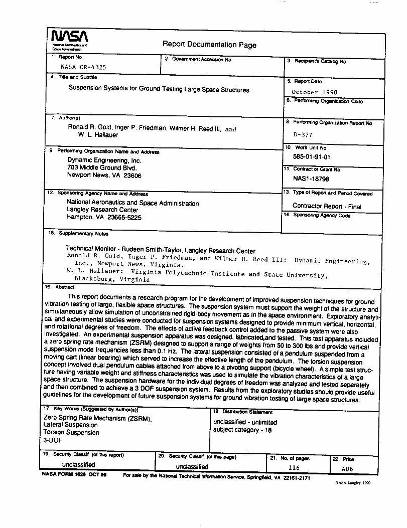
16,
..=.,.,,.=,., Report Documentation Page
I Repot1 No 2. Government A_ No
NASA CR-4325
4. T_e and Subtle
SuspensionSystems for Ground TestingLarge Space Structures
9.
Aumoqs)
Ronald R. Gold, Inger P. Friedman, Wilmer H Reed III, andW L Hallauer
Performing Organizalzon Name and Address
Dynamic Engineering. Inc.703 Middle Ground Blvd.Newport News, VA 23606
12 Sponsonng Agency Name and AG_,.¢_
National Aeronauticsand Space AdministrationLangley Research CenterHampton, MA 23665-5225
15 Supplementary Notes
3. Recq_enrs CataJogNo.
5. Report Date
October 1990
6. Performing Organiza_on Code
8 Performing Organcabon Report No
D-377
10. Work Umt No.
585-01-91-01
11. Conlract or Grant No
NAS 1 - 18798
13. Typeof R__=rporl_.and Period Covered
Contractor Report- Final
14. Sponsoring Agency Code
Technical Monitor-Rudeen Smith-Taylor, LangleyResearch Center
Ronald R. Gold, Inger P. Friedman, and Wilmer H. Reed III: Dynamic Engineering,Inc., Newport News, Virginia.
W. L. Hallauer: Virginia Polytechnic Institute and State University,Blacksburg, Virginia
Abs_a_
This report documents a research program for the development of improved suspension techniques for ground
vibration testing of large, flexible space structures. The suspension system must support the weight of the structure and
simultaneously allow simulation of unconstrained rigid-body movement as in the space environment. Exploratory analyti-
cal and experimental studies were conducted for suspension systems designed to provide minimum vertcal, horizontal,and rotational degrees of freedom. The effects of active feedback control added to the passive system were also
investigated. An experimental suspension apparatus was designed, fabricated,and tested. This test apparatus included
a zero spring rate mechanism (ZSRM) designed to support a range of weights from 50 to 300 Ibs and provide vertical
suspension mode frequencies less than 0.1 Hz. The lateral suspension consisted of a pendulum suspended from a
moving cart (linear bearing) which served to increase the effective length of the pendulum. The torsion suspension
concept involved dual pendulum cables attached from above to a pivotingsupport (bicycle wheel). A simple test struc-
ture having variable weight and stiffness charactenstics was used to simulate the vibration charactertstcs of a large
space structure. The suspension hardware for the individual degrees of freedom was analyzed and tested separately
and then combined to achieve a 3 DOF suspension system. Results from the exploratory studies should provide usefulguidelines for the development of future suspension systems for ground vibration testing of large space structures.
17 Key Wo,-,_ ($_m,_,___t=,'Jby Author(s))
Zero Spring Rate Mechanism (ZSRM).Lateral SuspensionTorsionSuspension3-DOF
19. =-¢_-J."dyCL',_._it (of this report)
unclassified
N-A-SAFC,_J 1626 OCT86
18. Distrib_T,,_3Stel_T,_-_
unclassified - unlimited
subject category - 18
zo. secure/c==_. (of_ pace) 2t No.of pag_u_nc___-_=-__!fied 116
For saleby _ NaliorwdTechnicalInformationSe_0Ce.SiwingfwWd,VA 22161-2171
22. Price
A06
NASA-Lmz_ey, 1990
-,,,