Embed Size (px)
Citation preview
THE EXTENSION AND APPLICATION
OF DIFFERENTIAL ANALYZER TECENIQUE IN THE SOLUTION
OF ORDINARY DIFFERENTIAL EQUATIONS.
by
Samuel Hawks Caldwell
S.B., Massachusetts Institute of Technology1925
S.M., Massachusetts Institute of Technology1926
Submitted in Partial Fulfillment of the Requirement
for the Degree of
DOCTOR OF SCIENCE
from the
Massachusetts Institute of Technology
1933
Signature of Author,
Certification by the Department
tKsT. gECO
14 SEP 1933
LI BR AP
~-~~~~~1
ACKNOWLEDGMENTS
For a period of three years, I enjoyed
the privilege of almost daily association with
Dr. Vannevar Bush in the developinent, and later the
operation of the Differential Analyzer. In these
formal words, I cannot fittingly acknowledge my
indebtedness to Dr. Bush as a teacher, friend, and
helpful critic, but hope that this thesis will show
to some extent that his hard work has not been
entirely in vain.
To my nimerous advisers of the Department
of Physics, and particularly to Professor Philip M.
Morse, Dr. L. A. Young, and Dr. W. P. Allis, I am
deeply indebted for their many suggestions and
criticiams, and their everlasting patience with my
naive conceptions in the field of atomic physics.
TABUT OF CQNTENTS
Page
Introduction
Chapter I.
Chapter II.
Application of the Differential Analyzerin Electrical Engineering
a) Machine transientsb) Electric circuitsc) Acoustics
General Applicationsa) Dynemics
The Problem of Three BodiesCosmic rays
b) Astrophysicsc) Miscellaneous
451523
2525374950
52546264
Chapter III. Applications in Atomic Physicsa) Atomic structure in the stationary
stateWave mechanics
b) Non-stationary state atomic problemsc) Potential field problems
Chapter IV.
Chapter V.
The Problem of the Self-Consistent Fielda) The Hartree methodb) An extension of Hartree's method for
the heliun-like at omsc) Procedure on the Differential Analyzerd) Control and reduction of errorse) Computationsf) Resultsg) Discussion of method and results
Sumary and Conclusionsa) Range of application of the present
machineb) Desirable additions to present equip-
mentc) Significance of the Differential
Analyzer methodd) Utility and significance of the work
in atomic physics
67
7275909599
100
122
127
129
131
Table of Contents cont'd.
PageAppendix A. Derivation of schedule used in applying
the method of least squares for the controlof accidental errors 133
Appendix 3. Method of fitting aapirical wave func-tions to the machine data 138
Appendix C. Calculation of the energy parameterfrom the equation of the wave function 140
Appendix D. Calculation of scale factors 142
Appendix E. Symbols 149
Bibliography 151
Biographical sketch 1515

INTRODUCTION
The developnent of any machine brings with it the necessity
of devising methods of using the machine in order to derive full benefit
from it. With a machine as comprehensive as the Differential Analyzer 1 ,
this necessity is a continuing one, for, except for certain general pro-
cedures, the method of using the machine is dependent largely on the
requirements of the problem in hand. To a certain extent, then, any
successful attack on a new type of problem will almost invariably leave
behind it a contribution to that aggregate of basic methods which con-
stitutes a technique.
Until about one year ago, exploratory work on the Differential
Analyzer related largely to the field of electrical engineering - a
natural consequence of the fact that the machine was developed by
electrical engineers. Other fields were receiving some attention, but
not to the extent that seemed desirable. This situation has now changed
considerably, and a real demand has arisen for the use of the machine in
other branches of science and engineering. In particular, the applica-
tion of the machine in atomic physics has been extended rapidly, and
much of the material of this thesis deals with this type of work.
In the field of atomic physics there was, and still is,
abundant opportunity for exploring the possibilities of attack by means
of the Differential Analyzer. The physicist has an assortment of the-
oretical rjethods - as developed by Heisenberg, Schrodinger, Dirac, and
others - from which he can set up the equations governing a given atomic
configuration, but with the exception of the hydrogen atom and the
1. See bibliography for all numbered references.
-2-
hydrogen-like atoms, he can obtain no specific solutions for those
equations. Approximate methods have, of course, been developed, and
give excellent results in a ntnber of cases, especially in those cases
where the answers to similar problems are known. As a last resort, the
method of numerical integration can be applied, usually with reasonable
success, and always with a great deal of labor.
In entering this field of activity, the writer did not first
make a general survey with the idea of picking a likely looking point
for attack. Rather he entered it in a spirit of inquisitiveness,
impelled by the fact that on at least three different occasions he had
told visiting members of the Physics Department staff that the Differ-
ential Analyzer could handle the differential equations of atomic physics
which they brought with them. On the fourth occasion, he not only ans-
wered "yes" again but decided that it would be highly appropriate to
prove that that answer was right. In February 1931 the Differential
Analyzer method was tried, and in accordance with the established custom,
it was tried first on the hydrogen atom. The success which followed
merely gave further evidence to support the growing tradition that almost
any method works with hydrogen.
The plan of attack developed in this first operation was fairly
simple. In fact, it was too simple because the desired result was known
analytically, and it was easy enough to make sure the machine was operat-
ing satisfactorily. Nevertheless, the work did show that it was possible
to attack the more difficult cases provided a method could be developed
to insure unifomiity of operation of the machine. The principal object
of the work to be described was, therefore, to investigate and enlarge
L
the range of application, adaptability and reliability of the
Differential Analyzer. In the course of the work, the writer, by
applying the philosophy of the machine method, was able to make an
improvement in the basic method of solving the problem chosen, and has
therefore made it a second object of this thesis to present as an illus-
trative example an extension of Hartree's method for obtaining the wave
functions of atomic configurations containing a nucleus and two electrons.
The presentation which follows id divided into four main sec-
tions. First, there is given an account of the methods and procedures
developed for handling problems in electrical engineering, including a
short resume of the progress made with the product integraph. This is
followed by a treatment of certain general problems of broad interest,
particularly the classical problems of three bodies and the more modern
cosmic ray problem according to the Lemaitre-Vallarta theory. In the
next section is presented a general discussion of various problems of
atomic physics from the point of view of Differential Analyzer technique;
this serves as a background for the final section which describes the
writer's work in this field.
Chapter I.
APPLICATIONS OF THE DIFFERENTIAL ANALYZERIN ELECTRICAL EfGIERING
In exnmining the work done in connection with the Differential
Analyzer in the field of electrical engineering, frequent reference is
found to the forerunner of this machine - the product integraph2 ,3, 4 .
Although relatively inaccurate and of decidedly limited range in compar-
ison with the present machine, the product integraph was a highly effective
instrument in the hands of the many men who worked with it. Some concep-
tion of the extent to which it was used may be gained from the fact that,
in electrical engineering alone, there were fourteen theses submitted and
seven papers (exclusive of papers describing the machine) published describ-
ing work in which the product integraph was used. It is appropriate to
include this material in the discussion which follows, because the work
originally undertaken on the product integraph has been continued and
greatly extended on the Differential Analyzer, and also because methods
and procedures developed in this earlier work have been to a large extent
applied directly to the present machine.
Most of the solutions carried out on the product integraph
which will be discussed here, were in the field of machine transients.
This program has been continued and enlarged on the Differential Analyzer.
Likewise solutions for both steady-state and transient conditions in elec-
tric circuits constitute another important group of electrical engineering
applications. More recently, the Differential Analyzer has been applied
to the solution of acoustics equations and it is expected that an exten-
sive program will be carried out in that field.
-5-
a) Machine transients
Solutions have been obtained on either the product integraph
or the the Differential Analyzer for machine transients problems of
three types, namely: machine behavior under short-circuit conditions,
machine performance under variable or suddenly applied load, and the
influence of various factors of design and operation on the pulling-into-
step ability of synchronous machines.
The first work on the camputation of short-circuit currents
was that carried out in 1927-28 by F. G. Kear, using the product inte-
graph5. Although the results of the immediate study were negative,
definite progress was made in two directions. First, during the course
of the study the machine as it existed at that time was altered to per-
mit treatment of more general types of equations. Second, the need for
a still more general type of machine and a more accurate one was shown.
Kearts description is especially vivid in dealing with the various errors
encountered in the product integraph and the means employed to eliminate
them*. These errors were, in fact, encountered and corrected during
the course of his investigation of short-circuit currents in alternators,
to the extent that the integraph became a machine sufficiently flexible
and reliable to turn out a steady stream of solutions of the two other
types of problems discussed below.
The short circuit problem received no further machine compu-
tation treatment until last year when C. Kingsley, .Tr. carried out on
the Differential Analyzer solutions of three-phase short-circuit cur-
rents on a synchronous machine6 * This work involved the solution of
* The equation -r, which Kear labelled "classic" because ofthe many d attempts made to solve it accurately on the pro-duct integraph was also the first equation solved on the Differ-ential Analyzer. The latter machine also failed to handle itaccurately until the "frontlash* unit was developed to eliminatethe backlash in the gear trains.
__~1
two semi-simultaneous equations. The first was a linear equation of
the third order, with constant coefficients, and from it the field
current transients were obtained. The second equation was used to
evaluate the armature current, using the field transients derived fran
the first equation. Although the first equation could have been solved
analytically, a separate Differential Analyzer set-up was made for it,
largely because of the time saved in plotting out the field transient
over a number of cycles. Since the coefficients were linear, no manual
operation was necessary and the solutions proceeded rapidly.
The problem of determining the perfomance of synchronous
machines under conditions of variable or suddenly impressed load was
treated rather extensively on the product integraph (see references
7 - 17 inclusive). Up to the present time none of this work has been
done on the Differential Analyzer*. Aside from the improvement in
the accuracy of the results which would be derived from a repetition
of this work, by using the new machine a distinct improvement in tech-
nique is possible in at least one respect. The type of equation used
in most of the previous studies was
+ P(g) d. + sin g = P0 + PI (1)dt12 1
It should be noted that the coefficient P(Q) is a function of the
angle Q. In order to introduce this variation on the product inte-
graph, the te P(Q) -- was plotted as a function of dQ for adtl dt1
* A repetition of scme of the work of Edgerton and Iyon8 is scheduledto be carried out by Levine and Snell. This is for the purposeof getting more accurate solutions.
-7 -
number of different values of 9. These plots were, of course, simply
straight lines. During the course of the solution one operator sta-
tioned at the output platen read off the values of 9 from the result
plot and called them to the operator following the p d versus -9dtl dtl
plots. The latter followed the line corresponding to the last value
of e called to him, and shifted from line to line in accordance with
the result.
On the Differential Analyzer the step approximation described
above is unnecessary. The machine is now sufficiently flexible so that
the variable coefficient can be continuously evaluated as a function
of its argument and applied to the first derivative as indicated in
the equation.
The same approximation was made in the earlier work on
pulling-into-step phenomena (see references 18 - 22 inclusive).
Recently, however, this work has been largely repeated and extended
using the Differential Analyzer (see references 23 - 26 inclusive) and
the approximation has been removed. It will be instructive to examine
the procedures used in the last series of solutions.
Before taking up this topic, it would be well to consider the
method used for classifying the results, this method having been devel-
oped originally in connection with the product integraph solutions.
It is apparen that the solution of a given problem on a machine like
the Differential Analyzer always consists of individual solutions of
particular cases. The variations between solutions are caused by
adjusting one or more of the parameters of the equation, or by alter-
ing the starting conditions.
-8-
In formal solutions, on the other hand, it is possible to
express a result so that by altering certain tems in the equation of
that result any of the desired solutions may be obtained. The utility
of machine solutions is enhanced greatly by any process which tendis
toward such generalization.
The method of generalization used in the pulling-into-step
problem (and also in the problem of variable or suddenly applied load)
proceeds frcm the equation*.
p + pd + PMsin L (2)~dt 2, dtL()
The coefficients Pi and PM are constant, but Pd is a function
of 9 (see equation (7), p.10 ). These coefficients depend only on the
machine design and vary widely between different machines. For any
particular machine the equation can be solved as given, but the results
thus obtained would be of little value in attempting to gauge the per-
fomance of another machine of different design. It is out of the
question, of course, to obtain solutions for each desired cambination
of design constants and load.
Fortunately, by a simple change of variable, the entire
picture can be simplified and the equation can be thrown into foin fram
which it is feasible to obtain a general set of solutions. Dividing
equation (2) by Pj, there results
e2 + Pd d_ + PM sin g , Edt 2 P dt P (3)
* In the equation as given, the tem PR sin 2Q for reluctance torquehas been omitted; this does not effect the procedure, and the
equation with it included will be discussed later.
-9 -
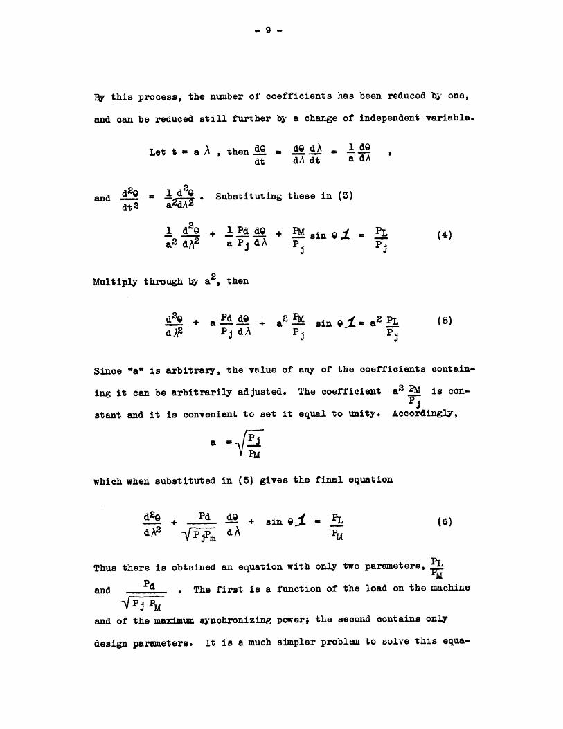
]r this process, the number of coefficients has been reduced by one,
and can be reduced still further by a change of independent variable.
Let t a ,then a dAddt dAdt adA
and - 2Q 1 d2 . Substituting these in (3)dt 2 a9
1 + . + sin . - (4)a2 dA2 aPj dA p P
Multiply through by a2 , then
d2 + a A + a P sin 9 a 2 PLdA2 Pj dA P P
Since "a* is arbitrary, the value of any of the coefficients contain-
ing it can be arbitrarily adjusted. The coefficient a2 PM is con-
stant and it is convenient to set it equal to unity. Accordingly,
a = PM
which when substituted in (5) gives the final equation
+ + sin 9.f1 =iL (6)d A2 \ dA
Thus there is obtained an equation with only two parameters,
and Ed . The first is a function of the load on the machine
and of the maximum synchronizing power; the second contains only
design parameters. It is a much simpler problem to solve this equa-
-10 -
tion for various values of the parameters thus combined, than to
solve it for various values of the individual constants.
The procedure described can be applied at least in part to
many problems and is a primary method of generalizing solutions ob-
tained on the Differential Analyzer.
In discussing the method of solving the pulling-into-step
equation, the most recent solution made by Edgerton (see reference 23)
will be taken as an illustrative example. He introduces a term due
to reluctance torque together with an expression which approximates
closely the variation of Pd with 0 and, after indicating two integra-
tions, obtains as his working equation
(;= - sin 91 - PR sin 29)dA - k(1 - b cos 2Q)dQ dAM
The information desired from solving this equation is the
maximum value of load ratio PL for which a motor having its field
switched on at a given angle will synchronize. From a series of such
results taken at different switching angles, the limiting switching
angle for any load ratio is obtained. The usual procedure is to run
a series of solutions with fixed switching angle and with varying PL ,
until two values of this ratio very close together are known, between
which the solution changes from the stable to the unstable type. This
procedure is repeated for a number of values of switching angle.
Edgerton made a radical change in the method, which elimin-
ated the trial and error feature entirely. He first obtained solutions
- 11-
PLat different values of --- for the steady-state slip versus steady-
PM
state angle, prior to field switching. A series of solutions using
the same values of PL was then made with the Analyzer running back-
wards. To start each of these solutions, the angle was set very close
to the unstable equilibrium angle and the slip at zero. The intersec-
tion of each of these solutions with the steady-state solution for the
same load ratio gave the angle at which the field would have to be
switched on in order to attain the unstable equilibrium angle. Thus,
except for accidents, each pair of solutions gave a useful result, and
the wasted effort inherent to the previous method was eliminated.
The Differential Analyzer connections used in this work were
quite conventional. Three integrators were employed, and the functions
(sin Q + PR sin 29) and k(l - b cos 29) were introduced from plots.
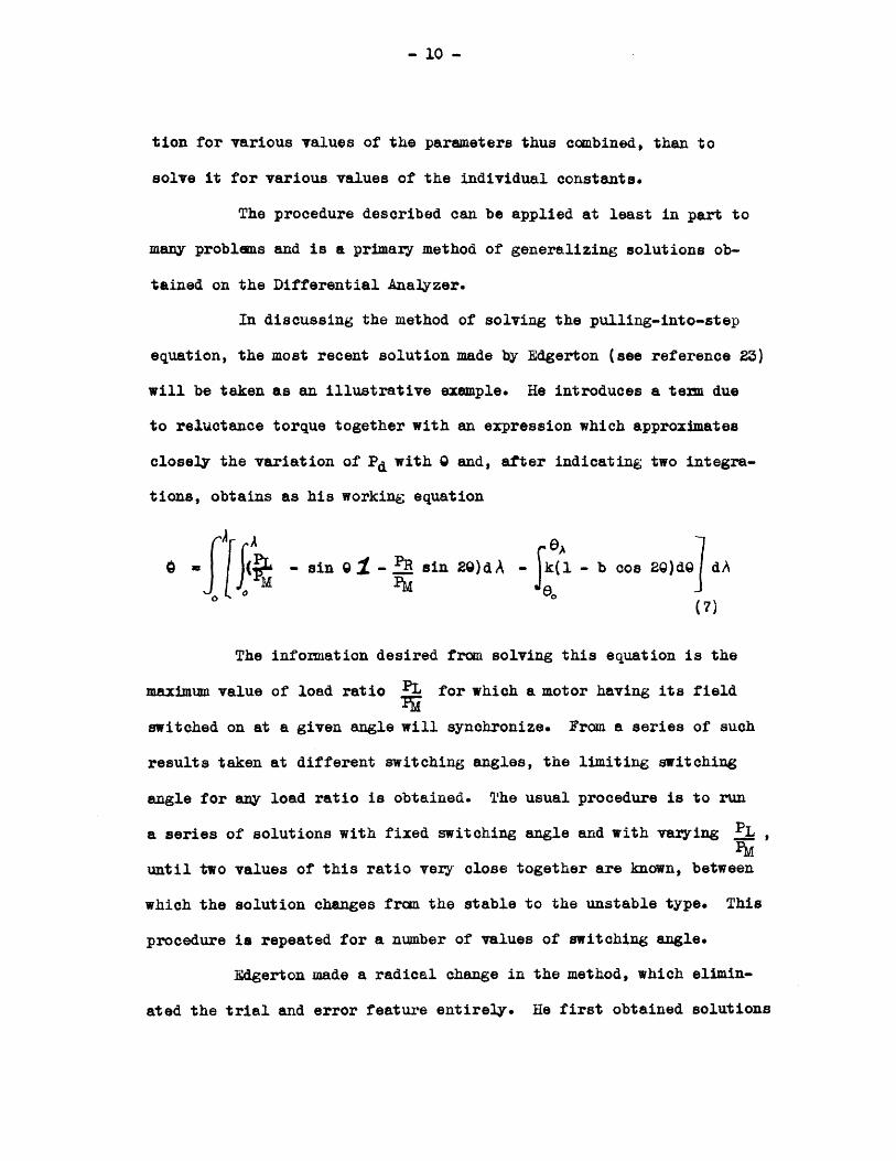
The schematic connections are shown in Fig. 1*.
Rramination of equation (7) shows that it is possible to
carry out this solution without using plotted functions, by the
following method. The second integral within the brackets is evaluated
formally giving the equation;
A A
sin 9.1 - sin 2G)dA
0 o- k(G - - sin 29 + 1 sin 29o) dA
2 2
* See Appendix E for the list of symbols used in these diagrams, andtheir meaning.

I
b 'A A ) d 8b crL)4
FIG. 1
-13-
Then substituting (2 sin 6 cos 9) for sin 29,
G JL(f -sin 91 - 2 P sin cos )dA (9)
-k( - b sin 0 cos 9 - 9 +1 sin 290 )] dA2
The equation now contains the functions sin 0 and cos 0 and these
can be obtained as the solution of the auxiliary equation
- cy, for which y a a sin 9 and c cos 9 (or vice versa).dg2
In order to carry out all the necessary operations with the six inte-
grators available at present, the terms of the equation must be some-
what rearranged. Also, the term , which is a constant for any
particular solution, must be integrated once formally in order to save
an integrator. The transformed equation becomes
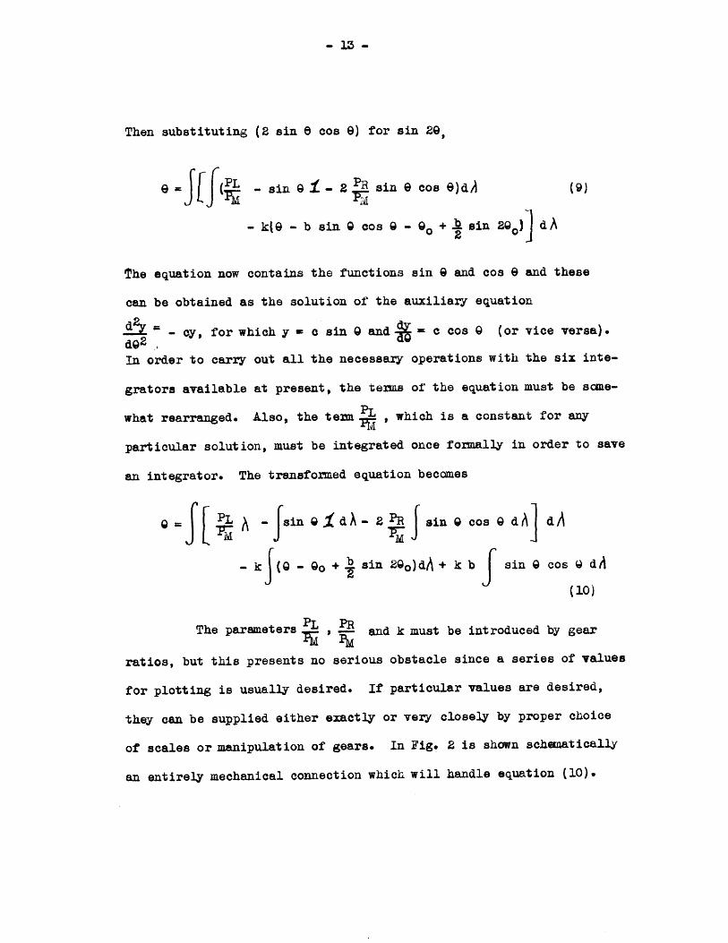
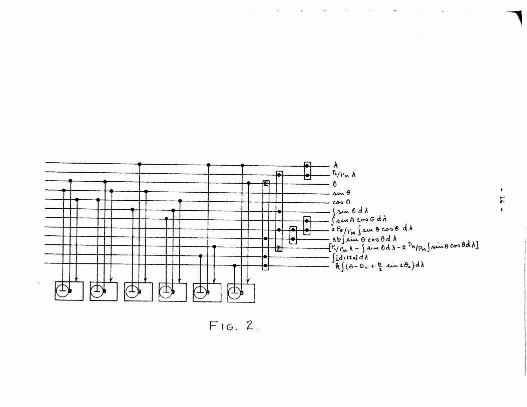
9 =$ A\ - sin 9 Id A-2 sin 9 cos 9 dA] dA
- kf(9 - 0o + sin 290)d/ + k b sin 9 cos Q dA
(10)
The parameters , and k must be introduced by gear
ratios, but this presents no serious obstacle since a series of values
for plotting is usually desired. If particular values are desired,
they can be supplied either exactly or very closely by proper choice
of scales or manipulation of gears. In Fig. 2 is shown schematically
an entirely mechanical connection which will handle equation (10).
[yy,~.~Vwyv
9T WYV+ 0 9f
v PLollI PIJf
x~ -q w W/
C F' wyt!
Q w -
VWd/
Z

- 15 -
b) Electric circuits
The ordinary differential equations of linear circuits are
not troublesome and in general the Differential Analyzer is not required
for their solution. Used merely as a means of plotting desired solutions
of higher order equations, it is to some extent valuable as a time saver,
but usually the analytic result is of more value. In cases where cir-
cuits contain non-linear elements, however, the situation is quite dif-
ferent, and the Differential Analyzer has a real part to play.
It is immediately apparent upon examination of the problem,
that the same difficulty exists as was found in the study of machine
transients. The solution for a particular case is readily obtainable,
but in order to permit any variation of the parameters of the circuit,
many separate solutions must be obtained. To a large extent, therefore,
the utility of the machine is limited to the study of cases of immediate
interest. This limitation appears not because of failure of the machine,
but because of the failure of the mathematical language used to set up
the equations. Furthermore, this limitation is present more or less in
every problem handled on the Differential Analyzer. It is particularly
troublesome in dealing with non-linear circuit elements because of the
wide variations of parameters which are possible and physically important;
in other problems, such as those of atomic physics, it gives little
trouble because only certain solutions have physical significance, and
continuous variation of the parameters is in many cases not required.
Some generality can be attained by extending the method of
changing variables described on page 5 . The following example has
been carried through to illustrate the procedure and also to show the

-16 -
6mount of repetition necessary to obtain solutions applicable over
a wide range of parameters in even a simple case.
Consider the circuit consisting of a constant resistance R
in series with an iron core inductance. If R includes the resistance
of the coil, and the inductance* is represented by L(i), then the
equation holding when a steady voltage E is suddenly impressed is
Ri + L(i) di= El (11)dt
or
i= .. dt- .J... i dt (12)JL(i) L(i)
Now introduce the change of variable
L(o) R
where L(o) is the value of L(i) at i = o, and equation (12) becomes
i L-*1d' - .- i d T (13)R L(i) JL(i)
The factor E is the steady-state current and must be treated as aR
parameter. Representing it by is, and dividing both sides** of (13)
by is
i d I dT (14)SL(i) Li
or 1 (1 - I)dr (15)SL(i)
* Hysteresis is neglected. L(i) is defined as N X 10-8, where $is in maxells and i is in amperes.
** This is peimissible because = is is constant for any particularsolution.
- 17 -
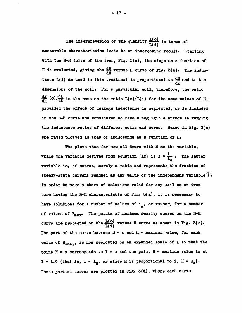
The interpretation of the quantity in terms ofL( i)
measurable characteristics leads to an interesting result. Starting
with the B-H curve of the iron, Fig. 3(a), the slope as a function of
H is evaluated, giving the . versus H curve of Fig. 3(b). The induc-dli
tance L(i) as used in this treatment is proportional to .B and to thedH
dimensions of the coil. For a particular coil, therefore, the ratio
d (o)/g is the same as the ratio L(o)/L(i) for the same values of H,
provided the effect of leakage inductance is neglected, or is included
in the B-H curve and considered to have a negligible effect in varying
the inductance ratios of different coils and cores. Hence in Fig. 3(c)
the ratio plotted is that of inductance as a function of H.
The plots thus far are all drawn with H as the variable,
iwhile the variable derived fra equation (15) is I a . The latter
variable is, of course, merely a ratio and represents the fraction of
steady-state current reached at any value of the independent variableT
In order to make a chart of solutions valid for any coil on an iron
core having the B-H characteristic of Fig. 3(a), it is necessary to
have solutions for a nuaber of values of is, or rather, for a nunber
of values of Baax. The points of maximu density chosen on the B-H
curve are projected on the L(O) versus H curve as shown in Fig. 3(c).L(i)
The part of the curve between H = o and H = maximu value, for each
value of B., is now replotted on an expanded scale of I so that the
point H = o corresponds to I = o and the point H = maximum value is at
I = 1.0 (that is, i = is, or since H is proportional to i, H = Hs)*
These partial curves are plotted in Fig. 3(d), where each curve
W

oyl (e/ : - oil _ _ __ _ _ _ __ _ _ _ oj 0_ _ _ _ _ _ _ _ _ _ _ _ _
I, WI 7i(0) 7
co~
HP9p)
(a)(~)
4

corresponds to a different value of maximin (steady state) flux density.
Using this last set of curves in equation (15), the equation
can be written more properly in the form
I' (I) L - I d7, (16)
thus indicating that the inductance ratio is used as a function of I
rather than i. The solutions of this equation are obtained for each
of the curves of Fig. 3(d), using the Anayzer connections of Fig. 4.
If a sufficient nuber of steady-state flux densities are
considered, then a chart of curves of I versus T can be prepared for
each kind of iron. By interpolation in such a chart, the current-time
curve due to constant E impressed in any R, L circuit using this iron
can be detexmined, within the limits of the asseptions set forth.
Up to the present time, very little work on the application
of the Differential Analyzer to general non-linear circuits (exclusive
of those eontaining vacum tubes) has been undertaken. Bachli and
Chibas 2 7 have studied a series-parallel circuit containing an iron
core inductance, and T. R. Saith28 studied an R, L(i), C series cir-
cuit. In both of these studies, the object was to ascertain the
response to sinusoidal voltages. In view of the engineering importance
of d-c. operated non-linear circuits (e.g. exciters, relays), further
study of the d-c. cases would seen appropriate.
* * * *
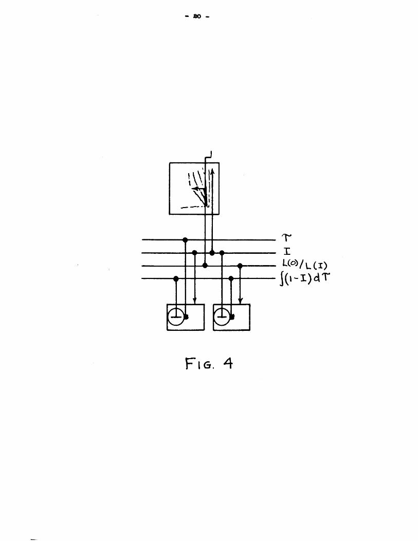
L(o)/ (L)
FiG. 4
III I I
rug

-u-rn
- 21 -
The vacuum tube as a circuit element has had increasing
importance during recent years. Its development and application has
proceeded largely on an experimental basis, with relatively little
analysis of an exact nature. The Differential Analyzer is of direct
aid in exact cmputation of the performance of vacuum tubes as cir-
cuit elements.
One of the principal difficulties in the machine treatment
of the vacuun tube problem is in the nature of the characteristic
curves which describe the tube. These curves form a surface* along
which the operating point shifts. On the Analyzer, this calls for a
three-dimensional input table if the representation is to be exact.
This is a possibility which cannot be overlooked; the table can be
constructed, but so far no procedure for constructing surfaces to
scale and with reasonable economy of time has been devised.
In order to avoid the difficulty, a closely spaced family
of curves is used, and the operator following the curves shifts from
one to another as the value of the third variable changes**. (This
procedure is the same as that applied in some of the machine transients
work on the product integraph (see page 6). While it must be recog-
nized that the method involves more or less abrupt changes, depending
on the skill of the operators, and that some degree of approximation
is thereby introduced, actual duplicate runs show such close repetition
of results that the procedure can be regarded as substantially exact.
* For the dynatron oscillator (Gager and McGraw29 ), only two dimen-sional characteristics are required.
** Radford set up a telephone system between the operator and anobserver who could read off the value of the third variabledirectly from a scale.
- 22 -
In the matter of generalizing the process, little can be
said at present. In the studies already completed (references 29, 30),
circuit constants were used diredtly with no attempt to combine para-
meters. Further work in this field is under way at the present writing
(references 31 - 33) in which ratios of parameters are used to some
extent. The problem is inherently non-general because of the wide
variety of tubes and circuits. This, together with the fact that un-
explained discrepancies exist between experimentally observed results
and those calculated by the machine, makes it necessary for the present
to apply the Differential Analyzer to the solution of particular prob-
lems. In other words, the principal functions of the Analyzer at the
present time is to aid in coordinating theory and experiment.
The machinery of the Differential Analyzer can be of use int
the evaluation of integrals of the form fA(t - A )E(A )d A , en-
countered in the study of linear networks with applied forces variable
with time. It is a straightforward integrating process which is carried
out for a sufficient number of values of t to give an adequate descrip-
tion of the variation. Although the process can be perfoned in more
elegant manner by machines of the type developed by Gould' and Gray35
and now under further developnent as the Cinema Integraph, the Differ-
ential Analyzer is useful as an alternative in important cases. This
problem has also a special interest because it was for the purpose of
carrying out such computations that Dr. V. Bush and Messrs. Gage, Craig
and Stewart built the watt-hour meter integrating unit which formed the
nucleus of the product integraph6. Another example of work of this
type (performed on the product integraph) may be found in the analysis
of three-phase transmission line transients carried out by Finley and357Williams
c) Acoustics
A study of the "Distribution of intensity in a sound field
bounded by a rigid hyperbola of revolution" was carried out on the
Differential Analyzer last year*. This is the first solution thus far
obtained of an acoustic field with boundaries which are surfaces of
revolution generated by curves other than straight lines; it is a fine
example of the power of the machine in handling problems which are
cmpletely unmanageable analytically. In addition to providing a
qualitative check of some recent experimental results obtained by
Hall8, the study furnished verification of the existence of standing
waves without external reflection - a condition previously suspected
from experimental evidence in this partioular type of field.
In setting up the problem, Professor Fey was able to separate
the variables of the original partial differential equations by making
a particular selection of the shapes of both source and boundaries.
The ordinary differential equations resulting were
-y B2 Cox2p + 1cot2 3+ - A (17)dP32 4 2 A (7
andA3 - Z [B2 sin 1 tah2 1+ A]da2 Z 4 2 (18)
* This problem was formulated and proposed by Professor R. D. Fay,to whom the writer is indebted for interpretative materialwhich has not yet been published.

In equation (17), which was the first treated, B is the frequency
parameter while A is an unknown parameter to be obtained from the solu-
tion*.
The means of determining A is contained in the boundary con-
ditions to be satisfied by the solution. For equation (17) these are.
at j=o, y = o, and at /6=/ (at the boundary), . cot,6,df3 2
Only the first of these conditions can be established when the machine
is started, so for a given starting condition it is necessary to vary A
until the required end condition is established. Once A is found for
a particular value of B, both parameters can be inserted directly in
(18) and that equation is then ready for direct solution.
It will be recalled that in the solution of the pulling-into-
step problem of synchronous motors, much the same process was carried
through. For a given set of conditions the Pi'PM ratio was varied over
a range in order to find the critical value, that is, the maximum value
for which the machine would synchronize. The requirement that the
machine should synchronize meant that the slip had to reach zero, or
in other words, a boundary condition was applied to the end of the run
just as in the case described above.
As will be brought out later, the same type of requirement
must be met in the solution of the equations of atomic configuration in
the steady state. In spite of the widely different characteristics of
the three physical problems, much the same mathematical idiom is used
in their description, and for solution on the Differential Analyzer, the
techniques have many features in comuon.
* The process for determining unknown parameters of this type was used
previously by the writer in studying the radial wave equation forthe hydrogen atom. o
Chapter II.
GENERAL APPLICATIONS
The many applications of the Differential Analyzer to prob-
lems of electrical engineering have been natural consequences of its
development by electrical engineers. But the electrical engineer must
express himself mathematically by language used in camnon with many other
sciences, and the machine he builds to carry out his computations is dir-
ectly applicable to other problems which are foxmulated by the same mathe-
matical processes.
In the discussion below, the work on atomic physics is omitted,
since it will be treated in detail in the following chapters. The prob-
lems taken up have in acme cases already been treated on the Analyzer;
the others are important in the literature and can be handled by the
Differential Analyzer method to advantage.
a) Dynamics
The problem par excellence of dynamics is that known as the
"Problem of Three Bodies". It may be stated*. "Three particles attract
each other according to the Newtonian law, so that between each pair of
particles there is an attractive force which is proportional to the pro-
duct of the masses of the particles and the inverse square of their dis-
tance apart: they are free to move in space, and are initially supposed
to be moving in any given manner 1 to detemine their subsequent motion."
This problem has been a subject of research for scme of the greatest
mathematicians and on it over eight hundred books and papers have been
* "Analytical Dynamics", E. T. Whittaker (1927), Cambridge. Chap. XIIIet seq.
- 28-
published within the last two hundred years. In the general form as
stated above, it cannot be solved in terms of any of the functions
known at present. It cannot be solved on the present Differential An-
alyzer either, because the machine does not contain a large enough
number of the required units. But a consideration of this classic
problem from the standpoint of machine technique is instructive, and
affords in a preliminary way a picture of what a more general Differen-
tial Analyzer must accomplish and how large a machine it must be.
The equations of motion of three bodies with respect to fixed
rectangular axes fonu an 18th order system, that is, there are nine
differential equations each of second order. Using dots over the co-
ordinates to indicate differentiation with respect to time, and chang-
ing the time scale so that the gravitation constant becomes unity, the
equations of motion with respect to fixed axes are.
E=M2 2 -XP Il + M3 X3 -i
Y2- Y1 + in3 Y3-yr12 r3B
1* 2 ~ + M3 Body 1.r123 r3
z? 2 Z2 -l + M 31 - X
r123 ryd
(1)
x2 = m3 Y3 - Y2 + mi 1 - '2r23 r 2 1
3
y2= 3 3- 2+ i 1 - 7r 5rg3 Body 2.
Z2 = m3 z 3 - Z2 + ml zi - z2r23 3 r 21p
-27 -
i -X13 + 2 - X33 =ml -r31. + M2 32 (1) contId,
Y73 = ml 1 -Y3 + m2 j3ody 3.-3-r313 r32
" M Zi -Z3 + m z -z3 1 3 2 -Z
Equations (1) may be reduced to a 12th order system by chang-
ing to a new set of axes with one of the bodies at the origin, and
expressing the relative motion or the other two with respect to it. No
loss of generality is involved in this procedure- the forces acting pre-
clude the possibility of there being any acceleration of the center of
gravity of the system as a whole, so that only the relative motion is
significant.
Let body 3 be located at the new origin; the coordinates of
the moving origin with respect to the fixed axes are (a,(3 , 2 ). The
new axes are allowed to move by translation only; that is, O'X' remains
parallel to OX, O'Y remains parallel to OY, and O'Z' remains parallel
to OZ, where the primes refer to the new system of co8rdinates. The
coordinates of any body with respect to the new system are then given by:
XU = zu ' + CX
yn - Yn' + (2)
zn = zn' +
and by differentiation
fn fl + Ct
" I99ZnU zn +
Substituting (2) and (3) in (1), and dropping the accents
x1 + a 2 r 23
1 + =m 2 rrl2
=m2 z2- 1
r 23
+ ~ y3 -Y 2y2 + =m3 r2,-r23
3
"+ z 3 -z 2z 2 + m -3r23
+E a i = X1-1313
r-3 3
t, if3
z3 + mir 331
+ M3 73-71
+ B1 Z3-Z1
r13
+ m 11-121 3
+ l r213+ m -1 Y
+ m Z1-Z213r21
+ mY2Y3r323
+ m 3
+ M 22-z32 . ;
Since in the new system, body 3 is fixed at the origin of
coordinates,
13 w Y3 " z 3 = 0,
and also3 = Y3 = 3 0
Making these substitutions in the last three equations of (4),
rj3 3
zi +
X2 + a
(4)
29
am 31r13
1
Ml Y
1'l
+ M2
r2
+ m2
r2
(5)
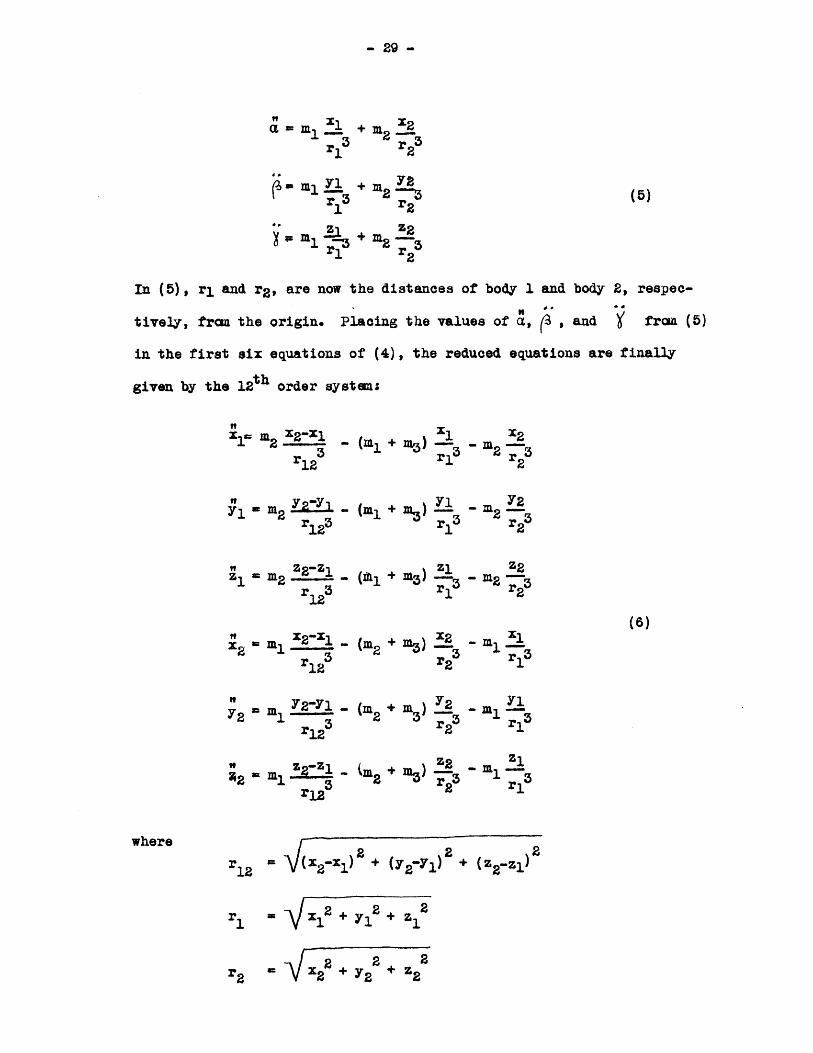
In (5), ri and r2, are now the distances of body 1 and body 2, respec-
tively, from the origin. Placing the values of , , and ' from (5)
in the first six equations of (4), the reduced equations are finally
given by the 1 2th order systems
r 1 23
y a 2 , - (.1 +r123'
-(mi + M) -3 - m2 3ri r 2
m3) - M2 '2ri 3 r23
1 = m2 - (Vl + m3 )
12
2 M 1 - (m2 + m3 )
=MY2-Yl (M --
y 2 =m 1 - n 2 + m3)
rl23
r 123
(M 2 + Mn3 )
3- m 3
3: -3MX3
r2 r23
X2 X1
r2 3 r
Y2 3 ulYl3r2 r
- m 12
r X 2 + y,2 + z2
r2 x22 + y2 + z2
(6)
where

-30-
The system of equations (6), although not of the lowest
possible order, is the best for attack by means of a Differential Anal-
yzer, to the best present knowledge of the writer. The equations can
be reduced to a system as low as the sixth order*. Analytically such
reduction is of value, but the complexity of the functions which must
be evaluated in solving the lower order system by machine methods is a
decidedly unfavorable factor. The eighth order system is somewhat better
in this respect, but still not as simple as that of the twelfth which has
been given. It did not seem necessary for the purposes of this treatment
to derive and analyze the intermediate orders. Possibly a ninth or an
eleventh order system is superior to the twelfth, and this possibility
should be thoroughly investigated before attempting an actual solution.
The principles and methods used here will be equally applicable to a
different set of equations.
Equations (6) can be somewhat simplified by again changing the
time scale so as to divide through ber either m 1 or m 2. Using the latter,
and recalling that the gravitational constant G has already been elimin-
ated in this manner, the new time scale is such that
t seconds, (7)
Br this change of variable, the final equations become
= xz~ - (A+B) " -Xi r 3 r 13 r7312 2(8)
A -l (l+B).2 XlX2 r123 - Z2r2 1 r
* of. Whittaker, loc. cit.

-51 -
(with similar equations for the y's and z's),
where
A and B= .m 2 m2
It should be noted that only two parameters appear, and these
are both ratios of masses so that the equations may be applied without
change to systems of either celestial or atomic dimensions.
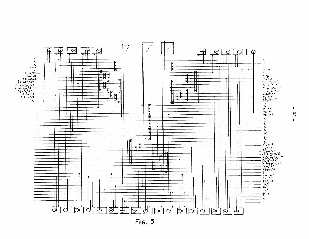
Fig. 5 shows schematically the machine connections suggested
for the solution of this problem. Gears in general are not indicated
but those necessary in order to introduce the various parameters of the
problem are shown. It will be observed that three input tables are
indicated as producing the necessary - 5/2 powers. These functions could
be produced by integrators as follows.
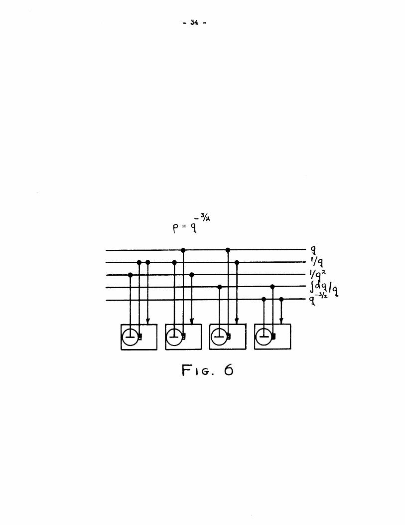
-s/aLet p q
- 3/2 q-/gdq
-/2 q 1
p dq
p - p (a)2 g
Now let, .q
dt 1
dq e
or q -f()2 dq (b)
x IjaI/r/at
(as- x,)/', A T
(a i A, Ie,' AtAS ,/r~LdT
It it I I
NEI I I I I
£0 _
_~i _ __Tz_
_ _~ Fi _ _I_
FiG. 5
-111 111 111 111- M
y
Y"
JyJaT(~ t e ))YJe4 a i
('-i,/ a
Al
(A+
A / Ir ?
S/r,.3 AT
/ 3
x- A.)
The mechanical connections in which the relations in (a) and (b) are
applied to produce the desired function are shown in Fig. 6.
Four integrators are required to produce only one of the
- 3/2 power functions, and since three such functions appear in equa-
tions (8) a total of twelve integrators would be required for this pur-
pose. This large number of integrators required, together with the fact
that reciprocal functions can be produced to better advantage from plots
makes it advisable to use input tables as shown in Fig. 5. This is
not a weakness in the method; a machine sufficiently comprehensive to
solve the three-body problem will certainly have automatic input tables
to introduce some functions.
The squares of distances which must be evaluated in this solu-
tion are produced using a single integrator for each square to be ob-
tained, by the simple and frequently useful method of integrating the
quantity to be squared with respect to itself*. It will be observed
* This method was first used on the Differential Analyzer in connectionwith a trial study of a problem in ballistics. Later, in a memoran-dun of Tune 1, 1931, Dr. V. Bush generalized the procedure by show-ing that a number of functions, among them the reciprocal . , couldbe produced by regarding them as solutions of auxiliary differentialequations. These equations were to be set up as in the example onpage 14, so that only integrators and adders would be needed forsolution. Guerrieri (ref. 39) carried out an S.M. thesis under thewriter's supervision, in which he derived the desired equations forsome forty functions. He also suggested the use of two integratorsand an adder for multiplication by use of the rule, uv =Judv + vdu.
In this same memorandum, Dr. Bush made another generalization ofgreat theoretical importance. He says, "Any differential equationwith variable coefficients (perhaps subject to rather broad condi-tions) may be regarded as a more complicated differential equationwith constant coefficients." This statement contemplates the pro-duction of any finite, continuous, single-valued function by the useof integrators and adders; various series expansions may be used forexperimental curves. The idea is one which has every prospect ofbeing developed into a powerful method in connection with a moreelaborate machine (see footnote, p.36).
33 -
Fi&. 6
that in all twenty-seven integrators are required for this solution, -
four-and-one-half times as many as are available on the present Differ-
ential Analyzer.
Various difficulties may occur in the course of a machine
solution of this problem. While a few of these difficulties may be
anticipated, a complete discussion is impossible because of the lack
of knowledge of three-body motion in the general case.
Consider, for example, the case of a sun and two planets, or
possibly a sn, planet and moon. For a given set of initial conditions,
the solution by machine would probably be quite straightforward. But
examining the initial conditions required, it is found that they con-
sist of the initial position and initial velocity of each body (except
the one fixed at the origin). These twelve numerical values plus the
values of the parameters A and B in equations (8) are necessary to
start each solution. Furthernore each of the fourteen quantities can
have an infinite nunber of values over an infinite range.
The immediate problem would be to restrict these ranges
either from practical or theoretical considerations. It is obvious
also that certain combinations become identical with others when co-
ordinates are interchanged and can be eliminated from the standpoint of
symmetry.
A further difficulty arises in those cases in which two of
the bodies come very close together, or even collide. The distances ri,
r 2 ,and r1 2 appear in the denominators of fractions,and if any of these
become zero, the corresponding terms in the equations become infinite.
- 36 -
This type of difficulty has been encountered on the present machine.
Two procedures can be suggested for overcoming it. Usually, in the
vicinity of such singularities it is possible to obtain accurate series
solutions which are reliable. In other cases, amaller terms may become
negligible, thus allowing simplification of the problem.
Although the Differential Analyzer cannot provide a general
solution of the problem, its individual nunerical solutions are worth
while, if only because of the novelty of getting a result, rather than
speculating about it. More can be expected, however, from systematic
charting of results, and it is not unreasonable to set out on a def-
inite program to determine, at least over a limited range, the varia-
tions in solutions due to systematic variation of parameters and initial
conditions. This is particularly true if a machine recently projected
can be used*. By using automatic methods for making connections, in-
troducing initial, conditions, and changing gears, it would be possible
to make real progress in carrying out exhaustive investigations of the
type discussed above.
iurther information might also be obtainable regarding
peculiarities of certain solutions of the three-body problem. If
instabilities were possible, they could well be examined. Although
it is not probable that general criteria for instability could be
established, the fact that there are unstable systems could be demon-
strated, if true, and something of their nature could be learned.
* * * * *
* Memoranda of Dr. V. Bush. Dec. 1, 1932; "Differential Analyzer;Specifications for an Improved Model"; Feb. 12, 1933, "Appendixto Specifications".

Considering the electron as a particle, the study of its
motion under the action of electric and magnetic fields is of importance
in many problems. Using the product integraph Sears" found the orbits
of an electron oscillating in the space between the filament and the
plate of a three-electrode vacuum tube, as part of his investigation of
the theory of the Barkhausen-Kurz effect.
More recently, Lemaitre and Vallarta~l have studied the equa-
tions of motion of charged particles moving in the magnetic field of a
dipole. By this means, they find analytically a variation of cosmic ray
intensity with latitude which is in agreement with recent measurements.
Their results were obtained by numerical integration of a rather complex
equation, and in order to extend the work recourse was had to the Differ-
ential Analyzer. An analysis and discussion of the steps taken in the
attempt to solve this problem on the machine is of interest, not only
because of the importance of the cosmic ray problem, but also because
of the splendid example offered of the methods used to extend the range
of the Differential Analyzer in difficult cases.
The equation to be solved, as given by Lemaitre and Vallarta
is2
+ C + sin 2 AdA
5 s2 ndAd 2 0os 2dxX2 . & 1 + C -sin 2 AdA .cos2A
x X2. x
or dividing through by x and taking the square root,
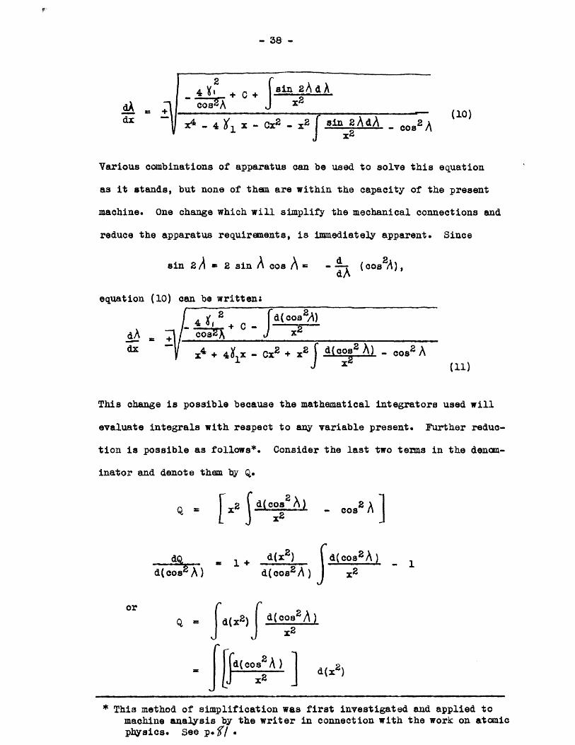
- 38 -
c sin 2A d Acosg-Ax2
A + (10)Varo4 - 4 us x -x2 . 2 sin 2A dA - cos2A
Various combinations of apparatus can be used to solve this equation
as it stands, but none of them are within the capacity of the present
machine. One change which will simplify the mechanical connections and
reduce the apparatus requirements, is immediately apparent. Since
sin 2 2 sin A cos A d (cos A),
equation (10) can be written;
4 2 dcos2dA + 2 -A)
dx ~ 4 + 491x - Cx2 + d(cos cos2 A(11)
This change is possible because the mathematical integrators used will
evaluate integrals with respect to any variable present. Further reduc-
tion is possible as follows*. Consider the last two terms in the denom-
inator and denote them by Q.
Q2 = x2 d(cos8A) - cos2A
d1 + d(x2) d(cos2 A)
d(cos2A) d(cos2 A) J 2
orQ = d(x2) d(co8a)
d(coA) ] 2
* This method of simplification was first investigated and applied tomachine analysis by the writer in connection with the work on atomicphysics. See pe g/
Also, since
14 = 2 .2 d (x 2)
andx2 = C d(x2)
the denominator of (11) can be written
- 4 x+ f[ 2x2 C +dcos2 d(x2
and the complete equation now takes as its final form
4 + - d(cos2cos2A x2
4 x + (2X2 - C + 2 ) d(x2)'~hJ J ~2(12)
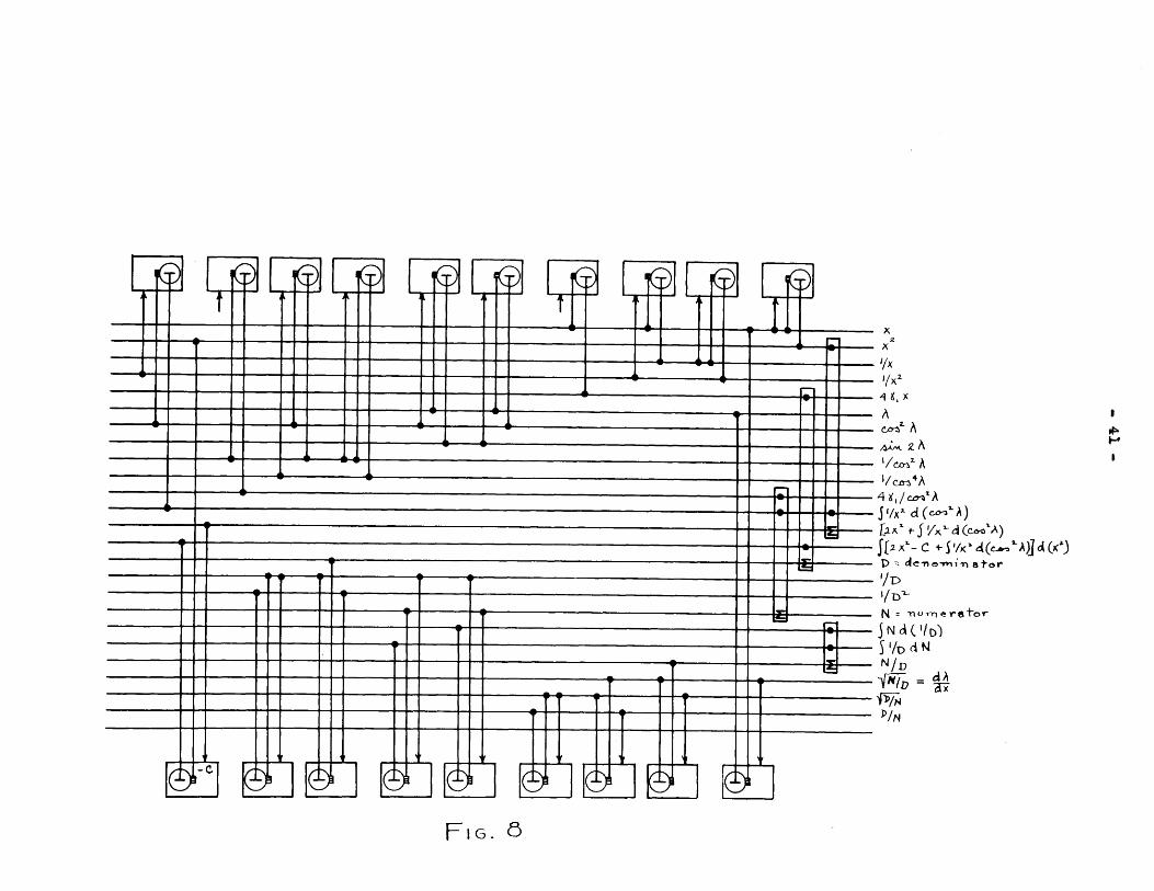
Fig. 7 shows schenatically the connections of the machine nec-
essary to solve (12). As far as is known to the writer, it represents
the form requiring the least amount of apparatus. For purposes of com-
parison, it is interesting to note the connections shown in Fig. 8, by
means of which the same equation can be handled using integrators, adders
and gears for all operations. A machine capable of handling the three-
body problem would, of course, contain the required nuber of units.
The results obtained in working with this equation on the
Differential Analyzer were most disappointing. Considerable time was
spent investigating peculiarities in the machine's behavior, and this
resulted in the discovery of two difficulties. First, the terns in x
appearing in the denominator combined so as to produce small differences
of large quantities. In order to correct this difficulty, it was necessary
- 39 -

x
2.
4 1, X
Aedo A
]~x'J/x a d(cd& A)
[ix'- c +Si/ d c&.Ad(x )N = -uJ erater
b =eleneoi nator
a A
FIG. 7
IL - --------- *"*-** ........ ..........
Fl G. (5.
'A
4/Z-S AA
/2 2- AA
I/
I/D
N/D
11 li 11 11 11
- 42 a*
to adapt the output table so as to serve as an input table on which
4 2was plotted the tena (x - Cx 4611C) as a function of x. Although
this removed the immediate trouble, much of the elegance of the method
was lost, and further trouble still remained.
It was now found that having started the machine, the solution
proceeded satisfactorily until the point was reached where the slope
dApassed through zero. From this point on, if no special procedure
was adopted, the machine stopped drawing a curve and simply described a
straight line parallel to the X-axis; that is, once it reached zero
slope, it continued with the same slope. The source of this peculiarity
was soon found, - not in the machine, but in the equation.
In equation (12) it may be observed that the slope is equal
to a fraction composed of functions of x and A in both numerator and
denominator. Hence the slope may become zero either if the numerator
becomes zero, or if the denominator becomes infinite. It so happens
that in this case the numerator becomes zero. Examining the numerator,
which is
4 + C - d(cos2 A)
the first term varies only with A , the second is constant, and the
third term varies only if A varies. Hence the numerator will change
its value only if A varies. But when the point of zero slope is
reached, not only does the numerator become zero, but it must stay
there, since A does not change. The machine goes on "dead center"
and draws only a straight line of zero slope as an answer. This solu-
-43-
tion satisfies the differential equation, but has no significance*.
An attempt was made to avoid the difficulty by arbitrarily
carrying the slope through zero in as continuous fashion as possible.
No consistency could be obtained, however, and the work on the problem
was discontinued to await further study. This study was to proceed
along three lines: first, to attempt to introduce a second derivative
into the equation in accordance with which the slope would be properly
varied; second, to study similar equations having known analytic solu-
tions (in particular, the Clairault equation); third, to seekareformu-
lation of the problem. The first method, although theoretically possible,
leads to no useful result because the final equation becomes too com-
plicated for the machine to handle it. The second method was somewhat
of a last resort and has not been tried. Recently, however, the writer
has had some success in reformulating the problem for the machine. Al-
though, it has not yet been tested on the machine, the method proposed
is not subject to the difficulty described above, because acceleration
terms are explicitly contained.
* The charged particle is moving in a magnetic field, and the solutionfound indicated it as moving in a direction at right angles to theaxis of the field-producing dipole. This cannot be true physically;the force produced by the motion must alter the path.
Mathematically, the difficulty is that the singular solutionA = const. exists, and at any point where dA = 0 , this solution
is tangent to the desired particular solu- U tion. No informationis supplied the machine to enable it to continue on the particularsolution, and since no further guidance is required for it to followthe singular solution, it proceeds to do so. Lemaitre and Vallartado not mention this difficulty in their paper; they encountered itin their numerical integration, but the true nature of the difficultywas completely recognized only after the machine study was attempted.

It seemed logical in attempting a reformulation of the prob-
lem to go back to the unreduced equations of motion. They express the
real physical problem, and since they contain the force terms explicitly
any solution of them must represent the motion of the particle under the
action of the forces present. The question is, can they be handled on
the present Differential Analyzer?
Lemaitre and Vallarta gave the equations of motion in polar
coordinates. Reducing these equations to the form in which they were
most easily handled by machine left them still far too complicated for
the present equipnent. Following this, the work of Carl St8rmer42*
was consulted for details of the methods he had used on the same prob-
lem in studying the phenomena of aurora borealis.
Briefly, St8imer sets up the equations of motion in rectangular
co8rdinates. Since the force acting on a charged particle in a magnetic
field is always perpendicular to its motion, the velocity is constant.
St8nner therefore changes to the independent variable defined by ds = v dt.
He then transforms to equations in cylindrical co8rdinates defined by:
x = R cos Z Z
y = R sin f
The motion is separated into two components, the first, motion in the
meridian plane, and the second, rotation of the meridian plane about
the magnetic axis. Since the rotation of the meridian plane can be
determined after the motion of the particle in the plane is known, only
the equations dealing with the latter motion need be considered immed-
iately.
* Lemaitre and Vallarta referred to St8imer's work both in their paperand in conversations with the writer. At the time of the first study,however, his equations had not been reduced to a form suitable for themachine. This step was taken by the writer in the present investigation.
- 45 -D
Neither the rectangular ooordinates nor the cylindrical co-
ordinates are quite suitable for reducing the problem to permit an
immediate machine study. Fortunately, Stonmer had made another change
of variables in order to simplify his own computation problem, and his
final equations are susceptible to machine attack.
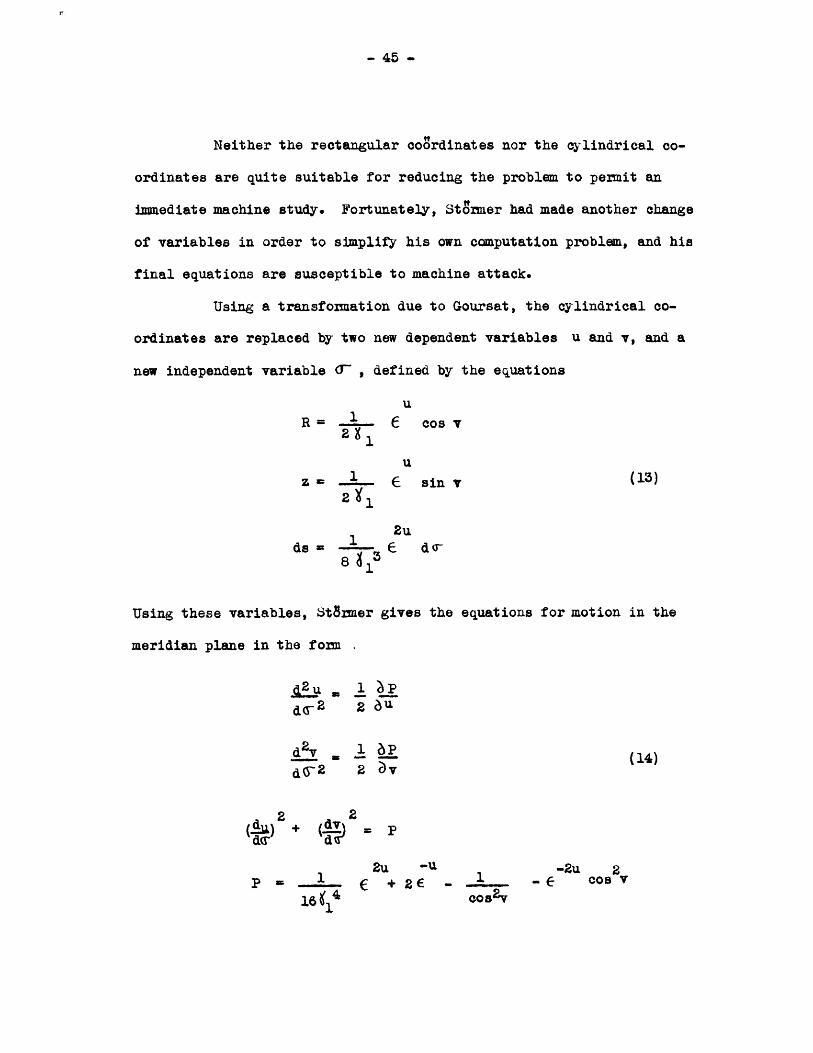
Using a transformation due to Goursat, the cylindrical co-
ordinates are replaced by two new dependent variables u and v, and a
new independent variable T~ , defined by the equations
u
R =6 Cos T
uZ =-- E sin v (1-3)
2 I
1 udo 3 -- E d T-
Using these variables, Stoimer gives the equations for motion in the
meridian plane in the fom ,
d6-V2 2U u
d2v 1 6P (14)
2 S2 2 hv
( ) + ( p
1u -u -2u 2P 1 + 2E - -- cosv
16' o2

-46-
Evaluating the partial derivatives, and indicating derivatives with
respect to G by dots, the required equations become
2u -u -Zu 2u= a - + 6 Cos V
(15)
= 6 sin v cos v -Cos v
where a =16
The third equation in (14) is not independent but can be derived from
the two given in (15) as will be shown later. It must be satisfied,
however, by the initial conditions. Hence only three of the quantities,
u, v, u and + can be specified arbitrarily in starting a solution.
To put equations (15) into forms which can be handled on the
present machine, two simple changes are necessary. Factoring out
E -2u in the first equation and (sin v cos v) in the second, and then
indicating an integration of each, they may be written
-tu 4u u 2U = (a 6 - + cos v)d-(
(16)
-2uv = sin v cos v ( C d -
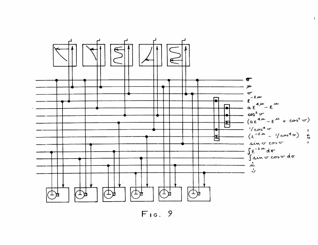
These equations can be solved with six integrators and five input
tables, which is just the limit of present equipment; Fig. 9 shows the
connections required. At the present writing a new attack on the prob-
lem, using these equations is being planned.
.6 .9'4
A i C -/ -
-P
-CrD + -fy 3 V-Ty * -0
r-5
..& r o
rvy W .r
..-........
(.
I.(Li
2u -u+ 2 6
2 -2uv = ff E
- 4cosv d( 2)
d(cos2V) 1coo2
Adding these it is apparent that the correct value of P is obtained.
The equations are of further interest, however, because in the form
u u -u+ 26 - cos v d(E
(18)
I -M 2 12u -e d(cos v) -
they can be set up on the present machine. But the old difficulty
again crops up, this time in a two-fold way, for if either u or v
reaches zero, it stays there. This time, fortunately, the source of
the difficulty is apparent. In deriving (18) the equations of (15)
were multiplied by u and v respectively. Hence the terms on both
sides of the equations all go to zero together, and the whole expression
- 48 -
The method of demonstrating the relation given in (14) that
'2 '2u + V
brings out equations which throw some further light on the difficulty
encountered with the Lemaitre and Vallarta equation. In equations (15)
I I
multiply the first equation by u and the second by v, and then integrate
both with respect to ~ . Since e dd6 = du, and dv - dv,
some of the integrations can be ccmpleted. When carried through, the
final results are
'2u a
(17?)

- 49 -
vanishes. Although the writer has not carried through in detail the
steps indicated by Lemaitre and Vallarta in their derivation*, a similar
process seems to have been carried out there.
The machine method indicated in Fig. 9 is by no means the best
obtainable# its only real advantage is that the present machine can
handle it. Unfortunately, all the integrating units are required for
strictly integrating purposes and none are available to generate func-
tions. With additional integrators available, the situation would be;
Number of additional Manual operatorsintegrators required
0 51 43 2
7 0
b) Astrophysics
In the general field of astrophysics, both the three-body
problem and the problem of the motion of a charged particle in a dipole
magnetic field (the earth's) must be included. These were discussed
under the heading of "dynamics" for the sake of generality.
It is to be hoped that investigations using the Differential
Analyzer will be undertaken in the near future along other lines. In
particular, the theory of stellar structure finds mathematical expression
to a large degree in the Endem** equation (and others)
. + = 0 (19)2d ( d n
* The derivation given in their paper (40) is very brief and containsnone of the detail steps which would furnish information on thispoint.
** R. Emden, Gaskugeln (Leipzig, 1907).
- 50 -
Much has been written on this equation and the nature of its solutions,
with but few actual solutions to write about. In one volume of a single
publication (Monthly Notices of the Royal Astronomical Society, Vol. 91,
1930-31) about ten papers appear dealing with this single equation or its
variations. The technique of its solution by the Differential Analyzer has
been explored by Bush and Caldwell 4 3 in a study of the Thomas-Fermi equa-
tion, which is the same as the Enden equation except for a change of sign.
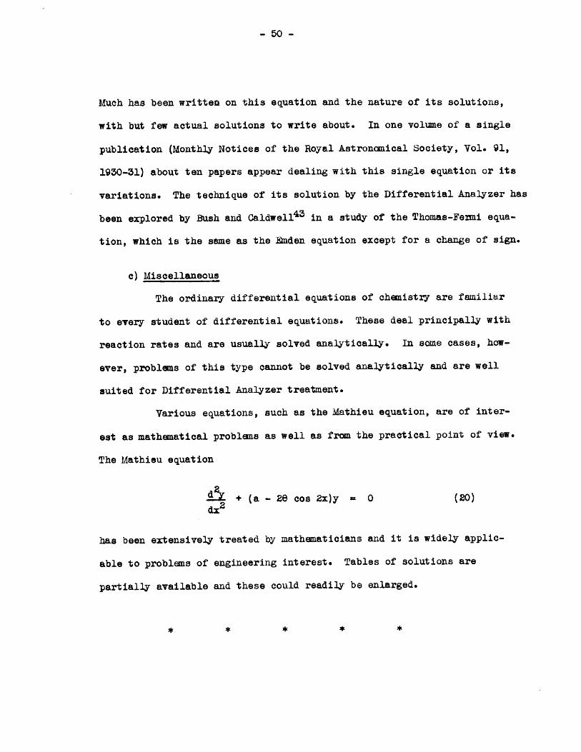
c) Miscellaneous
The ordinary differential equations of chemistry are familiar
to every student of differential equations. These deal principally with
reaction rates and are usually solved analytically. In some cases, how-
ever, problems of this type cannot be solved analytically and are well
suited for Differential Analyzer treatment.
Various equations, such as the Mathieu equation, are of inter-
est as mathematical problems as well as from the practical point of view.
The Mathieu equation
+ (a - 2e cos 2x)y = 0 (20)
has been extensively treated by mathematicians and it is widely applic-
able to problems of engineering interest. Tables of solutions are
partially available and these could readily be enlarged.
* *
I WNWINOWNW- MI
- 51. -
In these introductory chapters, besides reviewing much of the
important work carried out on the Differential Analyzer and its predeces-
sor, the Product Integraph, the writer has attempted to show by various
examples how the machine method may be adapted and extended to meet new
problans. In some cases the objective is reached if the problen can be
handled at all. The next step is to simplify the method, both with re-
gard to the nunber of solutions required and the complexity of the machine
connections. Finally, there comes the ultimate step of making the machine
do all the work, or as so aptly expressed by Dean Bush, ". . . . relegat-
ing to the machine those parts of the processes of thought which are
inherently mechanical and repetitive."
In the problen to be taken up in detail in the following chap-
ters, the first two steps have already been taken and the methods are
known for taking the final step.
Chapter III.
APPLICATIONS IN ATOMIC PHYSICS
a) Atomic structure in the stationary state
In the three decades which have passed since Planck intro-
duced his revolutionary idea of discrete, quantized energy states,
the science of atomic physics has developed to the extent that its
theoretical concepts are of practical interest to engineers in many
fields. Within relatively few years, the electron has come to play
an important role in everyday life; from it have come new industries
and others have been revolutionized as a result of the engineer's
deeper understanding of electronic phenomena.
The general historical development of this and other aspects
of atomic physics is treated in many books and papers on the subject .
Briefly, the commonly accepted model of the atom is, or was, that pro-
posed by Rutherford, in which there is a relatively heavy central core
or proton about which revolves one or more lighter particles called
electrons. These bodies are electrically charged, with each electron
carrying the same amount of negative charge and the proton carrying a
positive charge equal to the sun of the electronic charges. Most of
the theoretical analysis prior to 1925 was based on this simple model,
and it is still used to a considerable extent, at least for qualitative
purposes, at the present time. Much explanatory material in connection
with various phenomena of electronics, gaseous conduction, ionization
processes and photoelectric effects, etc., still deals with this
simple model.
- 53 -
For some time prior to the more recent developnents in
atomic theory, the shortcomings of this model were becoming apparent.
The quantum theory based on it had become more and more a patchwork
composed principally of classical mechanics and numerous arbitrary
rules which had been introduced in order to bring theoretical results
in accord with experiment. Furthennore, a number of cases had appeared
in which definite failure of the theory occurred*. Of these, among the
most serious was the inability to predict the spectral frequencies for
atoms containing more than one electron. Even for neutral helium, which
contained only one additional electron, the theoretical results were
definitely not in accord with experiment.
An additional and rather fundamental shortcoming of quantum
theory had been known for some time, namely, that even though the
theory might be patched up so that it would give reasonably accurate
predictions of the frequencies of emitted radiation, there was still no
way of calculating the intensity of the radiation. This situation was
inherent to quantum theory. No difficulty was encountered in computing
the amplitude of radiation from a simple oscillator, but quantum theory
postulated that radiation occurred only when an electron changed from
one orbit (or state of oscillation) to another. No laws governing the
intensity of the radiation produced by such a change had been formulated,
and in this respect at least it was quite evident that a radical change
in procedure was necessary.
The first step to correct the latter difficulty was taken
in 1925 when Heisenberg undertook to develop a method of using the
* Reference 44, Chap. VIII.
- 54 -
classical laws of radiation, and introduced a double subscript nota-
tion so as to make the intensity dependent on both the beginning and
end states of the electron. This method was studied and extended by
Heisenberg and others and has developed to the present-day matrix
mechanics. It has since been shown to give results equivalent to
those obtained by the later wave mechanics. Not only did later the-
ories make radiation intensity calculations possible, but they have
also been shown to give results much more nearly or exactly in accord
with experiment in many cases where the older quantum theory failed.
In 1924 L. de Broglie, in working out a new method for
computing energy levels, introduced the idea of a wave motion associ-
ated with electrons in motion. This idea was later amplified and
extended by Schrodinger in his original papers on wave mechanics.
As has been mentioned above, the results given by Schr8dinger's theory
are identical with those given by Heisenberg's. In fact, the two
methods are exactly equivalent in content although entirely dissimilar
in form.
* * * * *
The general problem of wave mechanics is to solve for any
particular case the Schrdinger wave equation*
2 + M2 (W - V) = 0, (1)
* Valid for stationary state problens in which the variation withtime is assumed to be simple harmonic.
- 55 -
where ) is the wave function, ik is the mass of the particle con-
sidered, h is Planck's constant, W is the total energy, and V is
the potential energy. This is, of course, a partial differential
equation and is not susceptible to direct attack by present machines.
Before any solution can be obtained, it is necessary to find Coor-
dinates in which the variables will separate.
In this discussion it will be assumed that the variables
have been separated properly, and that the equation for the radial
component of the wave function is given. This equation is an ordin-
ary differential equation, and in the case of hydrogen is written
1 d. (r2 ) . 1+ S+ V (W + .- )S= 0,r dr r 2 h2 r
(2)
where S is the radial component of P. It is customary to study
this equation after two changes are made. The first is to change
to the variable R = Sr. The second is to introduce new units such
that distance is measured in terms of the radius of the first Bohr
orbit (= 0.528 x 10- cmi.), and energy in terms of the ionization
potential of normal hydrogen (= 13.54 electron volts). These changes
simplify the form of the equation and the coefficients. For hydrogen,
the resulting expression is
dR + (E - 1(i +) + 2)R 0 (3)2 x2 x
Only certain particular solutions of equation (3) are
significant, and these are found by satisfying certain conditions
- 56 -
inherent to the physical problem. In the first place, the wave func-
tion 9) of equation (1) is presumably a quantity of scme physical
significance, and it is conceivably a measurable quantity. If so, it
must be finite throughout the entire range of variables. Since S is
a component of q), it must obey the same restriction, and hence R
must have the value zero at r = 0 (or x = 0) because R = Sr. Now as
r approaches 0O , if only the criterion of finiteness of S is applied,
the function R can become infinite, and under this condition it is
impossible to select a significant solution.
Other reasoning, based upon the physical interpretation of
the - function, furnishes a definite condition to be satisfied.
Not only must q) be finite over all space, but it must satisfy the
relation S iT)dV = 1, (4)
where T is the complex conjugate of 41 and dV is the volune element
of the particular co8rdinates in which 4) is expressed. If ' is a
real quantity, the condition of (4) becomes simply
2dv 1. (5)
In order that this be true, both 4) and its component S must become
zero as r approaches infinity. The related function R in equation (3)
must also approach zero as x approaches infinity; in fact, R itself
must satisfy the equationd(
I-R2 dx=1 (6)
I
- 57 -
Since equation (5) is linear, it is apparent that the absolute mag-
nitude of R is indeterminate. The actual scale of R is known only
after it has been made to satisfy equation (6), a process called
nonnalization.
The physical interpretation of the 9J -function fran which
the nonnalization integral (4) is set up is given in various fonas.
It is commonly accepted that the expression W dv represents the
probability that an electron is located in the element dv. Since the
wave equation is set up for a single electron moving in the potential
field V, if this probability is integrated over all space, the inte-
gral must equal unity because there is the certainty of one electron
being present. Thus equation (4) is written directly. In similar
manner, R2 represents the probability that the electron is in the
volume element between x and x + dx, and as written in equation (6),
the integral over all values of the variable x must equal unity.
Sumarizing, the conditions which a solution of equation (5)
must satisfy are. first, R must be zero at x = 0 and at x = CO ;
second, the function must be normalized. The Differential Analyzer
technique must be such as to produce solutions which meet these condi-
tions.
The second of these conditions is readily met in a large
number of cases, of which the hydrogen atom is an example. When the
equation is linear, there is no need to consider the question of
normalization until after the solution is obtained. The scale of the
wave function can be anything and satisfy the differential equation.
It is the nomalization condition which is then used to fix the scale.
It will be shown later that valid wave equations which are
non-linear can be written. In general the criterion is that if the
potential terms (in equation (3) the tems - 1(1 +1) + .- ) arex I
known functions of the independent variable, or functions which are
assumed to be known, the wave equation is linear. If, on the other
hand, the potential energy is not known as a function of the independent
variable and must be expressed in tems of the wave function itself,
the equation becomes non-linear. In these latter cases, the nomaliza-
tion condition must be satisfied by the immediate solution because the
scale factor of the wave function is no longer arbitrary.
There still remains the first condition, namely, R(0) = 0 and
R(O) = 0; this must be satisfied in any event. How is the machine to
be operated in order to satisfy this condition? Consider the equation
written in a slightly different form, namely:
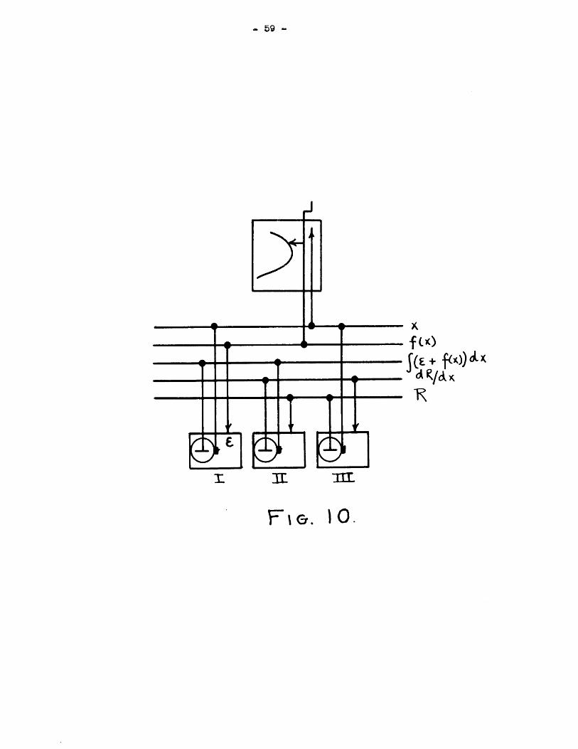
d2 + + f(x) R 0, (7)dx2
where f(x) is any known potential function and E is the term associ-
ated with the total energy. Fig. 10 indicates the machine connections
required if the equation is rewritten
-{ + f(x) R dx. (8)
Now suppose a solution is to be obtained satisfying the condition
stated above. Starting at x = 0, the abscissa displacement of the
fx)
fE+ )
SK~{~c~
9 : 1 'R I I
F e. 10.

- 60 -
input table will be set at this point, and the pointer will be
cranked to the initial ordinate. Next the integrator displacements
must be set to their initial values. Integrators II and III are, of
course, set at the initial values of R and .R respectively. R isdx
initially zero as required and can have any value (within the
limitation that the maximum available displacement on the lead screw
must not be exceeded) since its scale is arbitrary.
Integrator I as yet has no definite starting displacement.
It must be displaced in proportion to the temi 6 + f(x) , but only
f(x) is known initially. The total energy constant E is unknown and
must be guessed. Thus, one more condition (R (00) = 0) is to be ful-
filled and there is the one parameter E which can be varied as re-
quired. For a given f(x) there are only certain values of E which
will make R go to zero as x becomes infinite. These values of 6 are
known as the "characteristic values" or the "eigenwerte"; the correspond-
ing R(x)'s are called the eigen-functions.
Mathematical proof of the uniqueness of eigenwerte and eigen-
45functions is given in standard texts on wave mechanics . Considered
as a Differential Analyzer problem the role of the eigenwert as a
necessary adjustable parameter is quite apparent.
Certain difficulties appear when these solutions are tried.
Inaccuracies of machine operation are particularly troublesome. If,
for example, equation (3) were to be solved for a constant potential,
it could be written
d2i-- = R (9)dx
2
The solutions of this equation are exponential if K is positive and
sinusoidal if K is negative. In stationary state atomic problems, the
coefficient of R is negative near the nucleus and becomes positive for
larger values of radius.
Now suppose some slight error has appeared momentarily, suf-
ficient to change R from its true value by an amount A. The machine is
still connected to solve the equation, but the variable has been changed
and the equation can be written
d2 (R+A) = K(R +A) (10)dx2
Subtracting equation (9) from (10) there results the equation due to
the momentary error.
dA KA (11)dx2
The error term as thus given is of exactly the same form as
the desired function. In the range of x where K is negative any errors
which are introduced are sinusoidal and do not tend to cumulate rapidly.
In this region the operation of the machine is quite stable and results
can be repeated without difficulty. When K becomes positive, however,
the errors introduced accumulate exponentially and the situation is
critical. It is complicated by the fact that if the total energy is
not exactly an eigenwert, the R-function itself diverges toward either
plus or minus infinity exponentially. The problem of distinguishing
between an exponential error term and an exponential result is one of
- 62 -
the principal difficulties encountered; the method used to separate
them and to eliminate the error term will be described in the next
chapter.
In the discussion given above, nothing was said about the
form of the potential function f(x). The method outlined is straight-
forward and workable provided f(x) is finite throughout the entire
working range. It is characteristic of the atomic problem, however,
that the potential function becomes infinite at the nucleus where x = 0.
Hence, in general, solutions cannot be obtained in the simple manner
described above.
This limitation does not invalidate the argument which shows
that 4 must have a particular value in order to make R(OO) = 0. It
simply means that the starting conditions at some small positive value
of x must be specified, instead of those at x = 0. A small value of x
is necessary because over a small enough range, the solution can be
written in series form, and from this series the ratio of function (R)
to slope (dR/dx) can readily be obtained. With this exception, the
procedure is as outlined above.
b) Non-stationary state atomic problems
In addition to the stationary state problems there is a group
of wave problems in which the principal interest is in collision pro-
cesses; these may be classified as problems of the non-stationary atomic
state.
The equations governing the phenomena have been studied ex-
tensively on the Differential Analyzer, particularly by Prof. P. M. Morse
- 63 -
and Dr. W. P. Allis*. It would be impossible within the scope of
this thesis to discuss the collision problem adequately. It is inter-
esting, however, to note the form in which the equation most recently
studied was presented.
d 2 + (k + V(r)- =
drzr
-r - t+1 - + - -
+ 2 2 6 r f r Rdr + r 2r ER dr
(12)
The rather formidable problem of handling this equation on the present
machine was solved by taking advantage of certain symetries which
exist. If two new functions of r are defined by the equations
OCX= Jr 2E r dr040
2L6 r dr,
r
and the limits of integration are made uniform, this equation reduces
to
R + (k2 + V(r) - (/+1 ) R dr =
+ 2 +1 da R d -fd fRd x (13)
* A paper by these men describing the most recent work is to be pub-lished soon in the Physical Review. Also see "Quantum Mechanicsof Collision Processes", by Philip M. Morse, Rev, of Modern Physics,4, 577 (1932).
- 64 -
The final step necessary is to transfox the integral on the left,
writing for it
k2 + V(r) (+1)) R dr k2fr + R d V(r) (14)
where V (r) V(r) -- )dr (15)
This step is necessary so that the available number of integrating
units will be sufficient. It means simply that the integral in
equation (15) must be evaluated prior to machine operation.
Since the results of this work and the procedure followed
are soon to be published by Morse and Allis, no further discussion
will be given here.
c) Potential field problems
As indicated in section (a) of this chapter, the potential
field plays an important part in the solution of the wave equation.
In fact, in many cases, the problem is almost solved if the fom of
the potential function is definitely known.
The potential field problem is really one of detenmining
charge distribution. It is usually assumed then that the macroscopic
law
=frholds in atomic dimensions, and the potential is computed from it.
-65-
The justification for this assumption is that potential fields thus
calculated give results in accord with experiment.
In many of the problems of interest the potential field can
be written immediately. Thus, in the case of the hydrogen atom - that
"proving-ground" of all atomic theories - or the hydrogen-like atoms,
it can be written directly as
V(r) = -.r
where Z is the atomic number, and e is the charge on an electron.
This function when used in the wave equation leads to solutions which
check spectroscopic results.
Unfortunately, in the majority of cases, the form of the
potential function is notknown. Approximate methods are available,
however, and these would be made more useful if, for example, wave
functions were obtained for a wide assortment of empirical potential
fields. The Differential Analyzer is well adapted to supply such aids
to analysis.
The atoms with more than one electron are of particular
interest, and their potential field problems are difficult. If there
are very many electrons, the problem can be considered as a statistical
one in the manner of Thomas and Fermi. The Thomas-Fermi equation has
already been solved on the Differential Analyzer by Dr. V. Bush and
the writer, and the results are in the literature42,
Another method of treating the many-electron atom is due to
Hartree4 6 . This method is applicable where the fields are spherically
- 66 -
symmetrical - the so-called central field - or where they can be
assumed as central without introducing too much doubt. Consider the
case of the helium-like atoms in which there is a nucleus and two
electrons. Besides the assumption of a central field, Hartree assumes
that both electrons are identical and therefore have identical wave
functions. The wave function is obtained by solving the wave equation
for one of the electrons moving in the field of the nucleus and the
other electron. In order to find the component of potential due to
the second electron, its wave function must be known, and hence the
solution of the whole problem must be known. This, of course, is a
situation in which successive approximation methods are used, and
Hartree follows that procedure. His steps are
Initial field
Initial field corrected for electroncontributions
Solutions of Wave Equation
Distribution of charge
Final field
The desired solution is found when the successive cycles
of calculations repeat, that is, when the final field is the same as
the initial field. The final wave function is the one which is
characteristic of the self-consistent field.
In the next chapter, a new method is described for obtaining
the self-consistent field solutions. It has been successfully applied
in eight cases and the method has been developed to the point where a
solution for a single helium-like atom can be found in a reasonable
length of time.
-67-
Chapter IV
THE PROBLEM OF THE SFJE-CONSISTENT FIELD
a) The Hartree method
Two principal canputation processes are required to solve
an atomic problem by Hartree's method. First, a normalized wave
function is given and from it and whatever known charge distribution
is present, a potential field is camputed. Second, given this or
another potential field, the corresponding wave equation is solved
for a wave function which satisfies the boundary conditions of the
physical problem. It is assumed in referring to these processes that
the functions dealt with cannot conveniently be represented analytically.
Considering the first process as a machine problem, there is
given a normalized function S(r) which is a real function of r only.
This function is to be interpreted so that the charge density is given
by its square; that is, in the potential integral V = ,the
value 82 is to be substituted for Y .
The expression for the potential due to S contains two
terms, derived as follows. It is apparent that since the charge
density 32 is spherically symmetrical, the equipotential surfaces are
concentric spheres. Consider a spherical surface of radius r; the
charge of the electron is partly within and the remainder outside of
this surface. Due to the charge entirely within the surface, the
potential on the surface is given by the integral
r
~Vi JS2 0 'MTr r2 dr, (inner potential) (1)0
The second term, due to that portion of the charge which is outside
the surface is
00
S32* 4rr 2drJ r, (outer potential) (2)
r
The total potential due to the charge density 32 is the sun of (1)
and (2).
In the case to be studied, it is convenient to change the
variables of the original equation; the variable S is replaced by
and the scale of the independent variable is altered so that ther
417 factors of (1) and (2) are reanoved. Therefore, the working inte-
grals from which the potential is derived are given by:
V( 1 2 2 dxv(x) = 1 dx + x (3)
The evaluation of such integrals on the Differential Analyzer
is a simple matter. The connections required are shown in Fig. 11.
(See also Figs. 12, 13, 14).
Having found the potential energy expression, the second
principal part of the Hartree procedure, which is to solve the corre-
sponding wave equation, can be carried out as described in Chapter III,
part (a). The result is a new 4' which is used to compute a new poten-
tial in order to repeat the'process. With enough repetitions, the
condition will eventually be reached in which the q) used to compute
the potential energy is the same as that found by solving the wave
equation containing this potential energy expression. The name

*1 -i-
w/xp Af
X /) p
X6
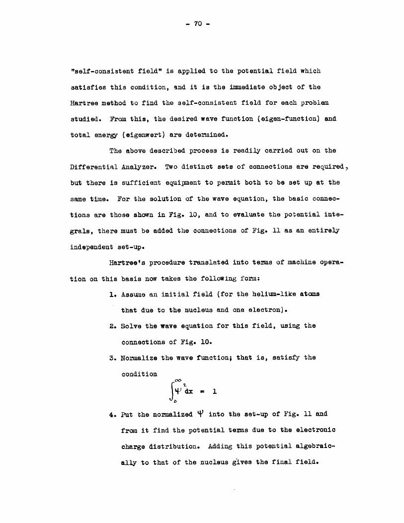
- 70 -
"self-consistent field" is applied to the potential field which
satisfies this condition, and it is the immediate object of the
Hartree method to find the self-consistent field for each problem
studied. From this, the desired wave function (eigen-function) and
total energy (eigenwert) are determined.
The above described process is readily carried out on the
Differential Analyzer. Two distinct sets of connections are required,
but there is sufficient equi.;ment to permit both to be set up at the
same time. For the solution of the wave equation, the basic connec-
tions are those shown in Fig. 10, and to evaluate the potential inte-
grals, there must be added the connections of Fig. 11 as an entirely
independent set-up.
Hartree's procedure translated into terms of machine opera-
tion on this basis now takes the following form;
1. Assune an initial field (for the helium-like atoms
that due to the nucleus and one electron).
2. Solve the wave equation for this field, using the
connections of Fig. 10.
3. Normalize the wave function; that is, satisfy the
condition
4. Put the normalized V into the set-up of Fig. 11 and
from it find the potential terms due to the electronic
charge distribution. Adding this potential algebraic-
ally to that of the nucleus gives the final field.
- 71 -
5. Compare the final field with the field first used.
If they are identical, the q) obtained in step 2 is
the solution desired. If not, replace the field used
in step 1 by that found in step 4 or by sane inter-
polated field and repeat until correspondence is attained.
Although this method offered no insunmountable difficulties
of execution, it was not a particularly attractive one. The idea of
having to carry out the calculations a piece at a time was bothersome,
probably because it seemed entirely out of line with the philosophy
of the machine method. The question kept arising, - why not connect
the two parts of the machine together so that the part in Fig. 10 fed
its 4' into the part in Fig. 11, and the part in Fig. 11 fed its poten-
tial right back into the part in Fig. 10 where it belonged? True, it
was then no longer the Hartree method, but it was evident that if the
potential function used in the wave equation was continuously gener-
ated from the solution of the wave equation, then every solution ob-
tained was a self-consistent one. Hence, if the machine could be
controlled so that a normalized, finite solution was obtainable, that
solution would be the same as would be obtained from the original
Hartree method.
There remained two questions. Could the problem be formu-
lated in its entirety, including the steps which in the first method
would be done on paper, and still be within the capacity of the 2
Differential Analyzer? If so, then could a solution satisfying all
conditions be obtained within a reasonable time?
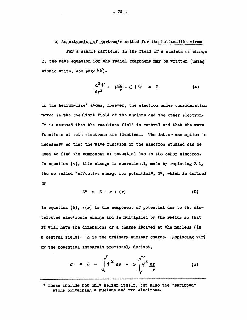
- 72 -
b) An extension of Hartree's method for the helium-like atoms
For a single particle, in the field of a nucleus of charge
Z, the wave equation for the radial component may be written (using
atomic units, see page 55).
d ( - - ) 0 (4)dr2 r
In the helium-like* atoms, however, the electron under consideration
moves in the resultant field of the nucleus and the other electron.
It is assumed that the resultant field is central and that the wave
functions of both electrons are identical. The latter assumption is
necessary so that the wave function of the electron studied can be
used to find the component of potential due to the other electron.
In equation (4), this change is conveniently made by replacing Z by
the so-called "effective charge for potential", Z*, which is defined
by
ZO= Z - r v (r) (5)
In equation (5), v(r) is the component of potential due to the dis-
tributed electronic charge and is multiplied by the radius so that
it will have the dimensions of a charge l~cated at the nucleus (in
a central field). Z is the ordinary nuclear charge. Replacing v(r)
by the potential integrals previous'ly derived,
Z*= Z - 2 dr - r j dr(6)
r
* These include not only helium itself, but also the "stripped"atoms containing a nucleus and two electrons.

- 73 -
It is more convenient in using the Differential Analyzer to use the
same limits of integration in both the integral teims of (6), so the
equation is expanded to
r 00 r
Z* Z - f q, d.r - r d2 + r (p 2
0rf r rf~ r (0 (7)
Now the integral f 2 is a definite integral and for any solu-
tion which is of physical interest it may be replaced by an unknown,
but finite, constant C. Since only these significant solutions are
to be retained, the substitution may be made imnediately, and Zo hence
becomesr
Z = Z - Cr 1 4 2dr + r qj2r (8)
Replacing the Z of equation (4) by the Z* thus computed,
and also introducing the changes of variable
x = Zr (9)
(10)
the equation to be solved becomes
x Xd2 )+ + 2 2 dx -fX0
Fx X Z ZZ
(The change of variable in (9) was introduced in order that the
maximum of Y would be reached in all cases near x = 1 instead of
- 74 -
getting closer to the origin as Z increased. Since 6 varies approxi-
mately as Z for this problem, the substitution of (10) was made in
order to introduce a parameter which varied only slightly in the neigh-
borhood of = 1. These changes were suggested by Dr. L. A. Young of
the Pbysics Department.)
Examining equation (11), it is apparent that the constant C
introduced adds no complication. The method of solving the wave equa-
tion requires that the value of be found by trial, and it is no more
difficult to do this for the value of ( + 2G). These values can
later be separated as will be shown. Of more immediate concern is the
fact that the equation is not linear, and hence the scale of 4 and
its derivatives is no longer arbitrary. Moreover, since the potential
is derived directly from Y , the wave function must be normalized as
it leaves the machine - it cannot be normalized in a separate operation.
Hence, the technique used in operating the machine must be such that the
resulting wave function is a normalized function which is zero at x = 0
and at x = oo
As has been shown before, the condition that q(0) is satis-
fied by starting with a zero value of 'P. Also, the parameter
( (+ -2) is available and this can be adjusted so that P (o) = 0.
The condition that W2 dx = 1 can be attained by varying the
starting slope, since now the size of at x = 0 has a direct
effect on the shape of C. Multiplying the initial slope by an
arbitrary constant no longer has the effect of merely multiplying
all values of V by the same constant.
M
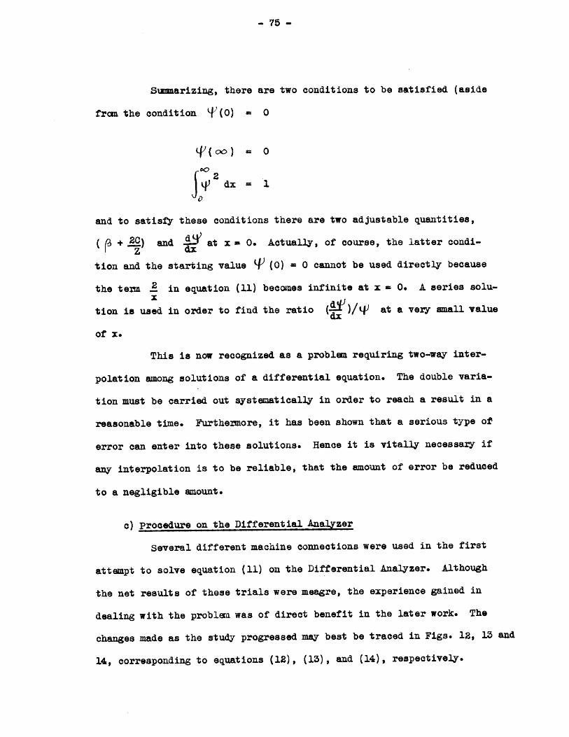
Sunsaarizing, there are two conditions to be satisfied (aside
frcam the condition T() = 0
(oco) = 0
2dx= 1
and to satisfy these conditions there are two adjustable quantities,
( + 2.) and 1L at x = 0. Actually, of course, the latter condi-Z dx
tion and the starting value q) (0) = 0 cannot be used directly because
the term . in equation (11) becomes infinite at x = 0. A series solu-
tion is used in order to find the ratio (.)/9J at a very small value
of x.
This is now recognized as a problem requiring two-way inter-
polation among solutions of a differential equation. The double varia-
tion must be carried out systematically in order to reach a result in a
reasonable time. Furthermore, it has been shown that a serious type of
error can enter into these solutions. Hence it is vitally necessary if
any interpolation is to be reliable, that the amount of error be reduced
to a negligible amount.
c) procedure on the Differential Analyzer
Several different machine connections were used in the first
attempt to solve equation (11) on the Differential Analyzer. Although
the net results of these trials were meagre, the experience gained in
dealing with the problem was of direct benefit in the later work. The
changes made as the study progressed may best be traced in Figs. 12, 13 and
14, corresponding to equations (12), (13), and (14), respectively.
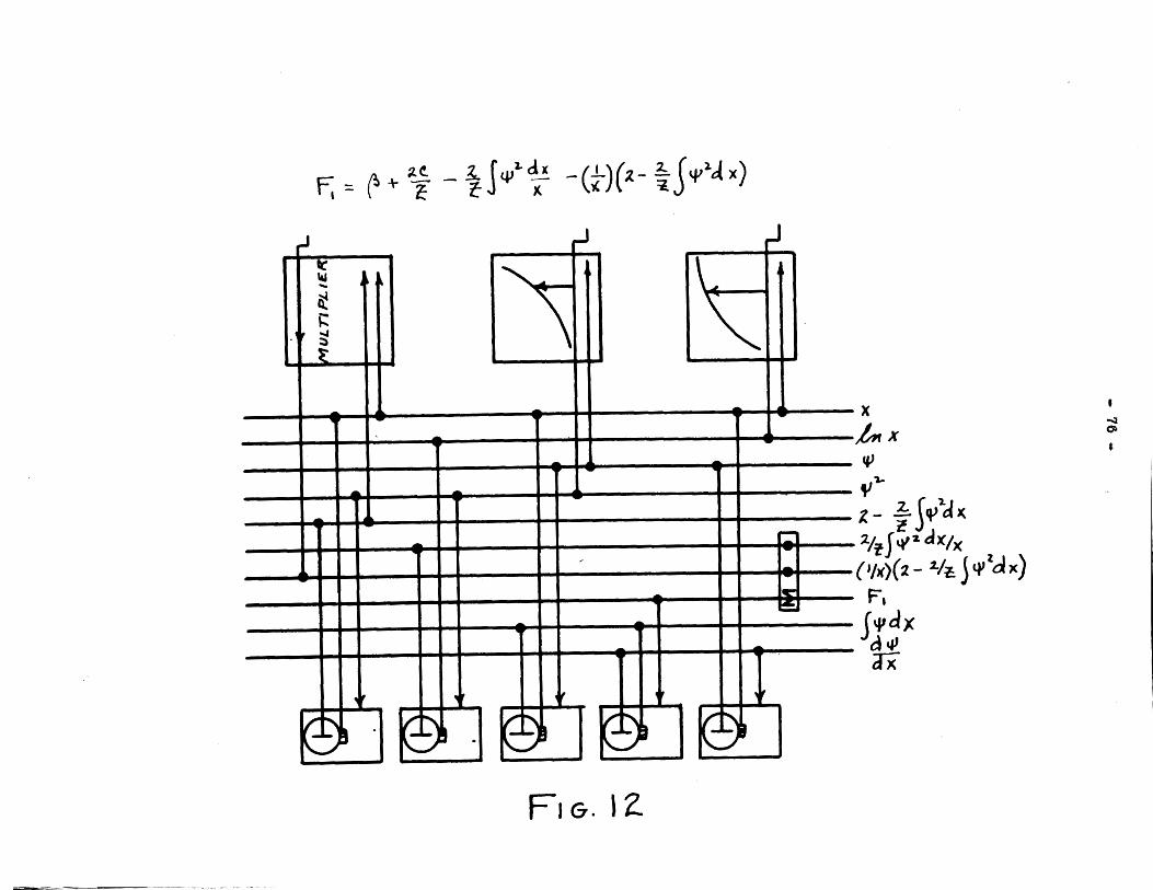
-21 9I .Sf
p
X/x' -
xwX
---
H
--r-_- -~ I
--i------
____ Vrrvr III~4
III IIIIII
F
(xpd)
T(bj 2
,rx Y 5 -e
AL
riL-- -
3(/b ---
--0
4 1- I
x Z + 7r

J7( 1z
X pth Ix p1
xp 4- _ -_ _
xp~~bL j
x -f) f
goal-"
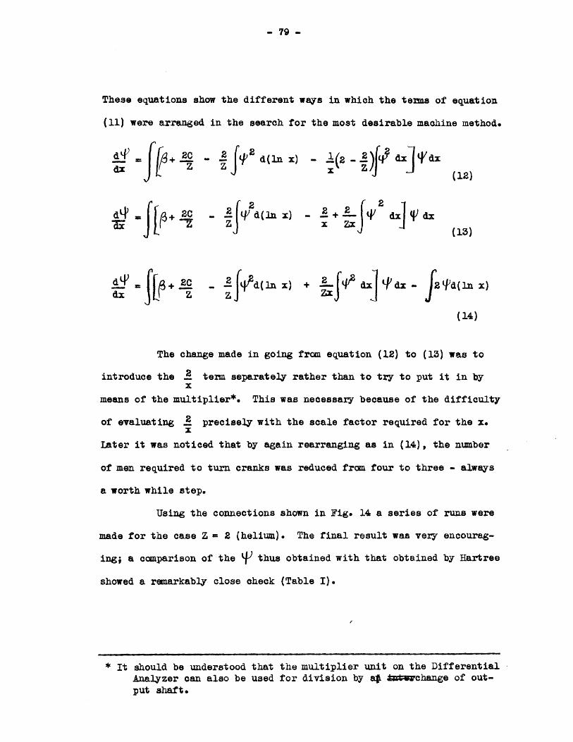
- 79 -
These equations show the different ways in which the tems of equation
(11) were arranged in the search for the most desirable machine method.
+ .r-d (Ix ) - f - x 9 dz (12)
dx f + 2 d (In x) -3+E dxj t dx
dx x
x JJ(13)
d' 2j+ Af d(In x) + 2 )dx dx -2q)d(ln x)
(14)
The change made in going from equation (12) to (13) was to
introduce the A term separately rather than to try to put it in byx
means of the multiplier*. This was necessary because of the difficulty
of evaluating A precisely with the scale factor required for the x.
Later it was noticed that by again rearranging as in (14), the number
of men required to turn cranks was reduced from four to three - always
a worth while step.
Using the connections shown in Fig. 14 a series of runs were
made for the case Z = 2 (helium). The final result was very encourag-
ing; a comparison of the q) thus obtained with that obtained by Hartree
showed a remarkably close check (Table I).
* It should be understood that the multiplier unit on the DifferentialAnalyzer can also be used for division by a tm*rchange of out-put shaft.
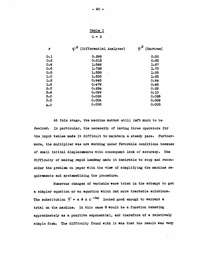
- 80 -
Table IZ= 2
£ 2r p2 (Differential Analyzer) 92 (Hartree)0.1 0.298 0.300.2 0.812 0.830.4 1.549 1.570.6 1.728 1.730.8 1.558 1.561.0 1.253 1.251.2 0.945 00941.6 0.479 0.482.0 0.224 0.222.4 0.099 0.103.0 0.026 0.0263.5 0.009 0.009
4.0 0.003 0.003
At this stage, the machine method still left much to be
desired. In particular, the necessity of having three operators for
the input tables made it difficult to maintain a steady pace. Further-
more, the multiplier was not working under favorable conditions because
of small initial displacements with consequent lack of accuracy. The
difficulty of making rapid headway made it desirable to stop and recon-
sider the proble on paper with the view of simplifying the machine re-
quirements and systematizing the procedure.
Numerous changes of variable were tried in the attempt to get
a simpler equation or an equation which had more tractable solutions.
The substitution 9- = a e x 6 -bx looked good enough to warrant a
trial on the machine. In this case e would be a function behaving
approximately as a positive exponential, and therefore of a relatively
simple foim. The difficulty found with it was that the result was very
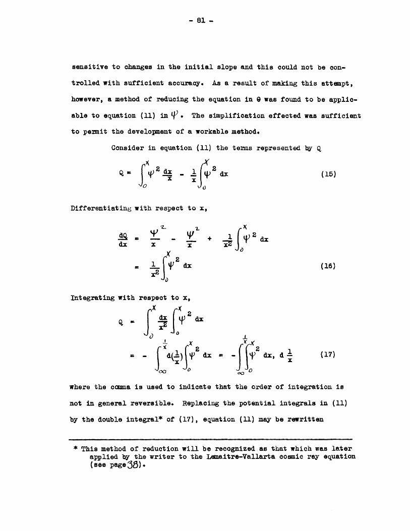
- 81 -
sensitive to changes in the initial slope and this could not be con-
trolled with sufficient accuracy. As a result of making this attempt,
however, a method of reducing the equation in G was found to be applic-
able to equation (11) in q). The simplification effected was sufficient
to permit the development of a workable method.
Consider in equation (11) the terms represented by Q
q, W d (15)
Differentiating with respect to x,
dx xX
3. 1P dx (16)X2j
Integrating with respect to x,
X 2
22
- d) dx = dx, d 1 (17)
where the cama is used to indicate that the order of integration is
not in general reversible. Replacing the potential integrals in (11)
by the double integral* of (17), equation (11) may be rewritten
* This method of reduction will be recognized as that which was laterapplied by the writer to the Lemaitre-Vallarta cosmic ray equation(see page38).

- 82 -
2 + - (P+ )-x0 (18)
This equationalthough little better in appearance, can be set up on
the Differential Analyzer in much simpler fashion, as shown in Fig. 15.
(See also Figs. 30 and 31 in Appendix D for details of the connections.)
Two important gains are made at once; only one operator is required
instead of three, and no multiplier is used at all. Profiting frCM
previous experience, the term containing A due to the nuclear chargex
is evaluated separately. For convenience in designing the connections,
equation (18) is rearranged in the fonm
_V + 3 C+ + f d )j dx-2
fF Sd S - (19)
It is interesting to observe that with two additional inte-
grators equation (19) could be solved by an entirely mechanical inter-
connection. An operator is required to introduce the function . ,x
and this can be done with two integrators* by setting them up to solve
the auxiliary equation - = - y2. This is the ultimate aim of thedx
machine method in all cases - to reduce the human effort required to
the point where only design and supervision are required, and to
simplify the procedures so that even this effort is a minimum.
The connections of Fig. 15 were found to be suitable and
using them the consistency of operation of the machine was much
These integrators would probably require special 4esign because forvalues of x<<l, the output shaft representing -... must rotate muchmore rapidly than the x-shaft. If the scale factors are altered tocampensate for this difference, the time required for solution withpresent integrators is excessive. A set of change gear boxes designedfor quick shifts would also be applicable in eliminating the difficulty.
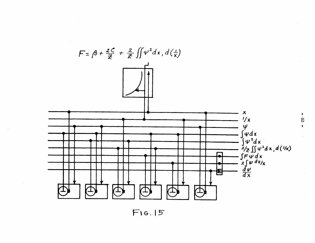
JJW~. UIIUIL I 1' 'I' Ut III IL I ~ II
- 2 ff(:2d)) j(I,
9' 3
f'dx2z/,Jqm SS(
Fl G. 15-
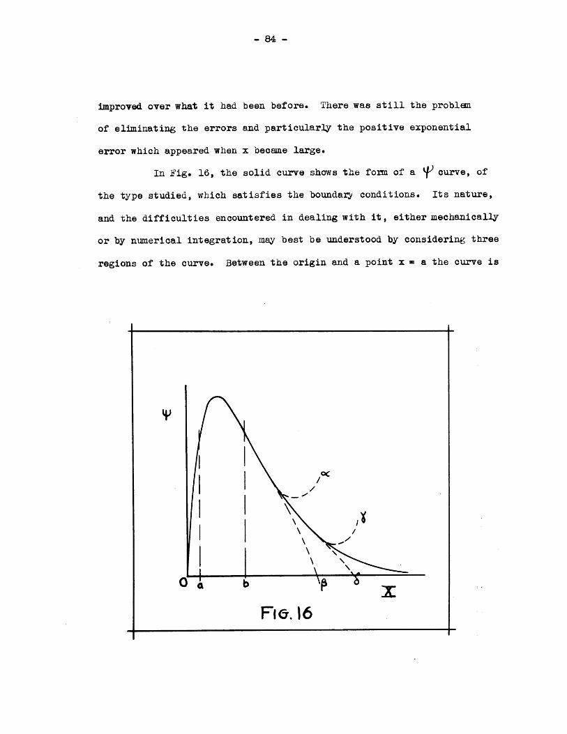
- 84 -
improved over what it had been before. There was still the problen
of eliminating the errors and particularly the positive exponential
error which appeared when x became large.
In Fig. 16, the solid curve shows the form of a IV curve, of
the type studied, which satisfies the boundary conditions. Its nature,
and the difficulties encountered in dealing with it, either mechanically
or by numerical integration, may best be understood by considering three
regions of the curve. Between the origin and a point x = a the curve is

- 85 -
essentially sinusoidal and is very stable. In this region the small
errors of machine operation have a negligible influence, on the average,
and consistency of operation is readily obtainable. In the region rrom
x = a to x = b, the solution changes from one which is essentially sinu-
soidal to one which is essentially exponential, and this region may be
described as a transition region. It is characterized by the tendency
of the solution to become unstable, to a degree determined by the values
of "a" and "b" which are assumed as the boundaries of the region. Here
the errors begin to accumulate exponentially and must be accounted for.
The region from x = b to x = cO is critical; the solutions are of
exponential form, as are also the errors. If the initial settings are
not quite right to produce an eigen-function, the solutions will turn off
exponentially toward either + oco or - o' as illustrated by the dotted
curves C' , 3 , , in Fig. 15. Moreover, this same thing will
happen in any case if the error is allowed to accumulate from the start.
It is apparent, therefore, that the inherent error must be controlled in
order that the behavior of the solution itself may be discerned.
It is useful in order to visualize the workings of the method
more clearly to consider what procedure would be necessary if an ab-
solutely perfect machine were used so that no errors of operation could
appear. The solution cannot be started at x = 0 because of the singular-
ity in the potential at that point. In order to start at some small
value of x an analytic solution over a anall range near the origin must
47be known. The solution used was
53/2 -(1 - m)Xi 2(l - --.- )
16Z(20)

- 86 -
(The use of this expression for q was suggested by Dr. L. A. Young.)
It was used only to obtain the ratio at x = 0.02. Differentiating
(20) and dividing this result by (20), the ratio is
.- (1- -..) (21)X 16Z
and for x - 0.02,
4= + -- (22)16Z
All solutions for the same Z were started at x = 0.02 with the same
value of , as given by equation (22). This satisfied the condition
that 4)(0) = 0.
Working with a perfect machine, it would now be necessary to
choose a value of ((+ ,,C) and run a series of solutions with differentZ
starting slopes until one was found which did not run off to either
+ c>O or - 00 , but followed a course similar to the one shown in Fig. 16
by the solid line. Even with a perfect machine which introduced no error,
this would be impossible, because for a given value of (f+ .2 .) theZ
initial slope (and hence the initial function) must have a value equal
to some particular number, with no tolerance allowed. For any finite
range of adjustment, the number of possible settings of an index is
infinite, and the probability of setting an index at one particular
point out of an infinite number is zero. Hence the statement that even
with a perfect machine, the desired result cannot be obtained exactly.
- 87 -
In spite of this difficulty, the solution satisfying the
boundary condition 4-' ( cO) = 0 can be found with sufficient accuracy.
As the critical value of slope is approached, the solutions proceed to
larger and larger values of x before they begin to diverge. Now if two
solutions are obtained, corresponding to two slightly different starting
slopes, such that at some large value of x (in practice x > 8) one
diverged toward + co-and the other toward - v< , the true solution would
be known within very close limits since it would lie between them. As a
matter of fact when the critical value of slope is known to lie between
two values which lie very close together, it is found that over a large
range of x the corresponding solutions are abost identical, and for all
practical purposes the true solution over this range can be obtained by
averaging. After the trial solutions begin to diverge, however, the
location of the true solution becomes doubtful.
The method of obtaining the true Y at large values of x
depends upon representing the two trial solutions by empirical functions
for values of x > 5. Since most of the charge of the electron is in
the region between x = 0 and x = 5, an approximate expression for (/2
beyond x = 5 is satisfactory provided it fits the observed points within
a few per cent*.
From the form of the equation, it has previously been shown
that the solution for large x is exponential. The desired solution must
contain only negative exponential terms since it must approach zero as x
approaches infinity. A trial solution very near the true solution must
* A one per cent error in fit, if always in the sane direction, wouldthrow the entire solution off about 1/20 of one per cent.
- 88 -
contain also either additive or subtractive positive exponential terms
to account for the divergence toward + 0 or - oo.
From these considerations, the form of the enpirical function
was chosen to be*
Bx DxA C- + C C (x > 5) (23)
Accordingly, this expression was applied to the trial solutions by using
a sufficient nutnber of observed values to determine the values of A, B, C,
and D. (See Appendix C for the method employed.)
The results of these calculations were as follows;
1. In all cases one of the exponentials turned out to be negative,
and the other positive.
2. For trial solutions diverging toward + c:,0 , the positive
exponential was additive; for those diverging toward -o3
the positive exponential was subtractive.
3. Canparison of the expression for two trial solutions
going toward + v0 and - c00 respectively, showed that both
had negative exponential terms of the same order of magnitude.
From each pair of oppositely diverging trial solutions a pair
of negative exponentials would be obtained by discarding the positive
exponential terms. An average of these negative exponentials provided
a satisfactory end region of the solution, satisfying the condition
q)(00) = 0. As a matter of fact, it was found that if the solution
could be pushed beyond the value x = 8 before either q) became zero(solution diverging to - CX0) or before V became zero (solution
* A better form would have been E= AGBx - CeDx, but this possib-ility was overlooked at the X time of carrying out the calculations.
- 89 -
diverging to + c6 ) that either type of solution could be used in
establishing the true solution without finding the oppositely diverg-
ing type. In the latter case, the positive exponential ten was re-
moved as described*.
Thus far a single solution satisfying the requirements at
x = 0 and x = 00 has been obtained, using a perfect machine. Now the
solution must be examined to see if it is normalized. It would be a
rare accident to get a normalized solution on the first attempt so
some provision must be made so that this condition can be controlled.
It will be noted in Fig. 15, that the output of one of the integrators
is jq) 2 dx, and this output displaces the disc of another integrator.
During the last part of the solution, this integral hardly changes,
particularly if the solution is of the type which goes to -oo. Hence
this integrator displacement serves during machine operation as a
fairly reliable guide as to whether the solution is above or below the
required nonalization. (Later, during computations, the final evalua-
tion of the normalization integral is obtained by Simpson's rule from
x = 0 to x = 5, and by integrating the negative exponential sguared
from x = 5 to x = c4 ). Having found one solution which is above or
below normal, the value of (p+ -0) is decreased or increased, and the
entire procedure repeated. A little experience soon shows how much
the eigenwert should be changed in order to produce another solution
which is slightly on the other side of the normal solution. The ob-
ject is to get two finite solutions very close together with the
normal solution between them.
* It should be remembered in this treatment assuning a perfect machine,that in the actual case the positive exponential term may be partlydue to error of operation. The entire term is discarded in anycase.
- 90 -
The final step is to evaluate dx for each solution
and then to interpolate between the two so that for the final curve
this integral has the value unity.
d) Control and reduction of errors
Before starting any important work on the Differential Analy-
zer certain precautions against systematic and gross error must be taken.
Unless they are subjected to severe overloads or damaged, the integrators
give little trouble. Plotted functions must be carefully drawn and
checked and all scale factors must be verified after the machine connec-
tions are designed. Similarly, after the machine has been connected, all
connections and gearing must be checked against the drawing. Bearings
must be oiled to reduce friction and all drives should be tested to make
sure there are no slipping set screws. Frontlash units must be inserted
in every drive in which the direction of rotation reverses; these are
adjusted to compensate the backlash present before any runs are made.
These routine precautions are adequate protection in most cases against
errors arising within the machine. Although no such protection is avail-
able against gross human errors in using the machine, these errors usu-
ally have no serious consequences because it does not require much
ialIvariation to make the solutions of different, equations behave very
unreasonably, and the machine frequently shows signs of distress.
The accidental errors encountered are due principally to
small errors in initial displacements and to irregularities in follow-
ing curves manually. These can be somewhat reduced by care and skill,
but in general this is not sufficient. Irregularities of curve follow-
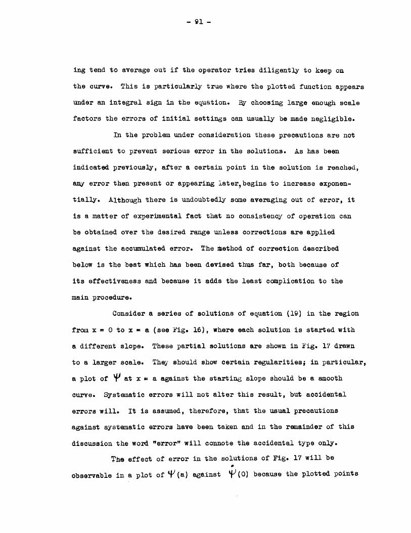
- 91 -
ing tend to average out if the operator tries diligently to keep on
the curve. This is particularly true where the plotted function appears
under an integral sign in the equation. By choosing large enough scale
factors the errors of initial settings can usually be made negligible.
In the problen under consideration these precautions are not
sufficient to prevent serious error in the solutions. As has been
indicated previously, after a certain point in the solution is reached,
any error then present or appearing later,begins to increase exponen-
tially. Although there is undoubtedly some averaging out of error, it
is a matter of experimental fact that no consistency of operation can
be obtained over the desired range unless corrections are applied
against the accumulated error. The fiethod of correction described
below is the best which has been devised thus far, both because of
its effectiveness and because it adds the least canplication to the
main procedure.
Consider a series of solutions of equation (19) in the region
from x = 0 to x = a (see Fig. 16), where each solution is started with
a different slope. These partial solutions are shown in Fig. 17 drawn
to a larger scale. They should show certain regularities; in particular,
a plot of Y at x = a against the starting slope should be a smooth
curve. Systematic errors will not alter this result, but accidental
errors will. It is assumed, therefore, that the usual precautions
against systematic errors have been taken and in the remainder of this
discussion the word "error" will connote the accidental type only.
The effect of error in the solutions of Fig. 17 will be
observable in a plot of 4F(a) against V(0) because the plotted points
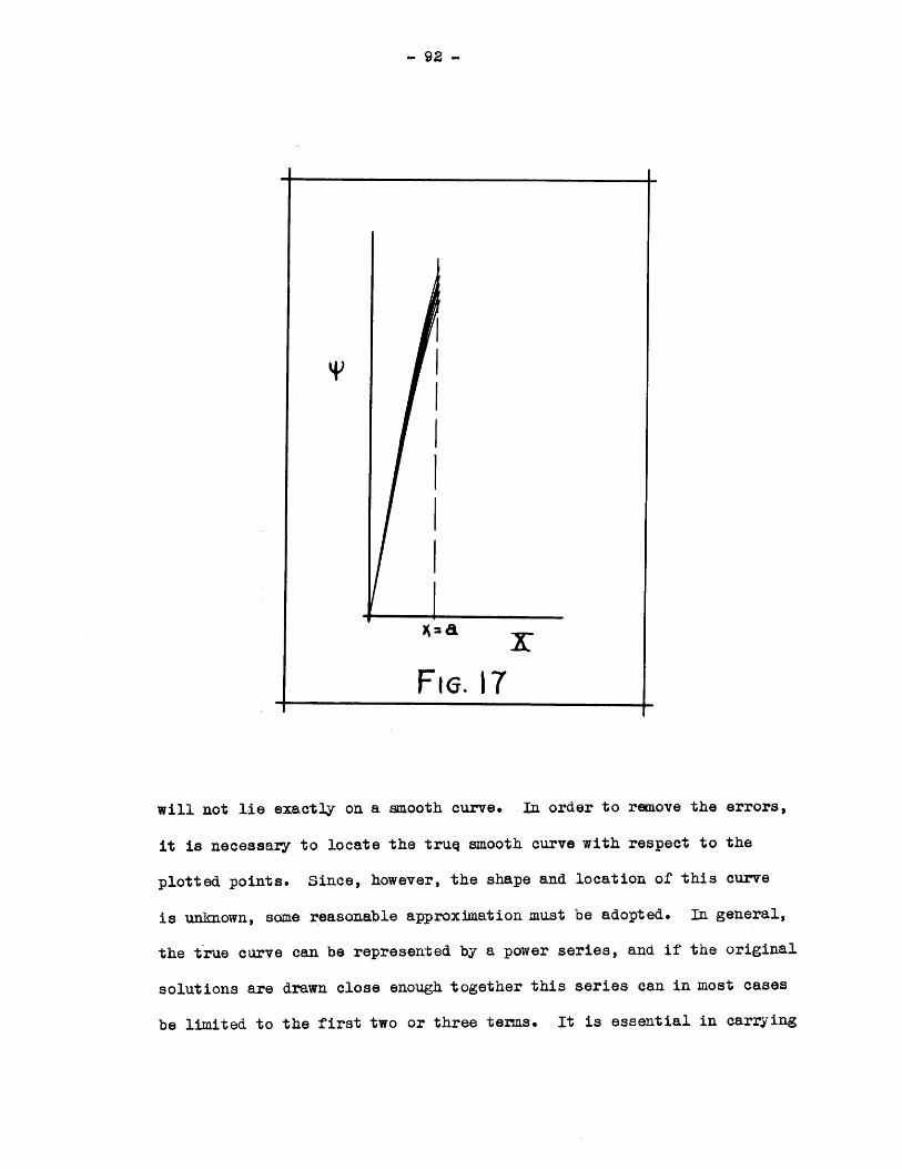
- 92 -
will not lie exactly on a smooth curve. In order to remove the errors,
it is necessary to locate the true smooth curve with respect to the
plotted points. Since, however, the shape and location of this curve
is inknown, some reasonable approximation must be adopted. In general,
the true curve can be represented by a power series, and if the original
solutions are drawn close enough together this series can in most cases
be limited to the first two or three terms. It is essential in carrying

out this method that the initial variations be of limited range so
that the end results always have a linear or parabolic variation.
Now although the exact position of this curve cannot be
detenained, it is possible to locate it in its most probable position.
This is accanplished by finding the equation of the curve (straight line
or parabola) by the method of least squares. The equation thus obtained
is used to calculate the corrected values of the variable - in this case
the 4)(a) of Fig. 17, but in general any of the variables of the problem.
These corrected values of the variables are now used as starting points
for the next region, at the end of which the process is repeated.
Translated into the language of machine operation, the rinal
procedure may now be given.
1. For a given fixed value of ( + 20), chosen to give a
nonnalized solution as nearly as possible, compute initial
settings for five runs, varying the initial slope by equal
small intervals. These solutions are all to start at
x = 0.02 and the ratio /f is to be kept constant at
its computed value.
2. -vithout recording any results, run the five solutions out
to the point x= 0.5 and stop the machine. At this point
read and record all integrator displacements.
3. Using the schedule method derived in Appendix A, compute
by least squares, the most probable values of the inte-
grator displacements.
- 93 -

4. Using the values computed in step 3, continue the
solutions through the second region, stopping the machine
at x = 2.2. Again read and record all integrator dis-
placements.
5. Repeat the cgmputations of step 3 on this last set of
readings.
6. Continue the solutionsusing the corrected displacements
just found. If the range of initial variation has been
properly selected, one or more of these five solutions
will diverge toward + C0 and the other toward - 00.
7. Interpolate between two adjacent but oppositely diverging
solutions until a solution is obtained for which neither
qA' nor ( reach zero before x = 8. Record this solution
from x = 2.2 to x = 8.
8. Make the same inteolation at x = 0.02 and record the
solution from there to x = 0.5.
9. Repeat at x = 0.5 and record to x = 2.2 (Note that the
starting conditions at x = 0.5 are interpolated from the
data obtained in step 5.)
10. From the result of step 7, read the magnitude of
PV 2 dx and deteraine whether the solution is above
or below nomnal. If this reading is very near unity the
final value is uncertain, and the estimate may be wrong.
This does not matter because the recorded solution will
then be very near the desired result and extrapolation
can be usedif necessarywith safety.
- 95 -
11. Repeat steps 1 - 10 with a new value of /+ 2G to correctZ
or slightly over-correct the normalization.
Thus two sets of data are obtained, bracketing the nonnalized
wave function, and in both sets the solutions are run out far enough
that the remaining positive exponentials, due either to accunulated
error or incorrect eigenwerte, can be eliminated by camputation.
e) Camputations
The results obtained fram the machine consist, for each value
of Z, of two sets of partial curves; both satisfy the condition W(0)i:O,
neither show marked tendency to diverge until after the point x = 8 is
reached, and the normal solution lies somewhere between them. Fig. 18
shows the form of the curves; in order to indicate how the curve is
started fresh at the beginning of each region, the accunulated error
has been exaggerated. The solid lines show the curves as they are ob-
tained from the machine and the dotted line shows the position of the
desired curve; regions are designate. by the roman numerals. The steps
taken to compute the final results from these data are the followingl
1. Fit the curve in region IV to the expression
1/ = ABx + CCDz and discard the positive exponen-
tial part of the result. The remaining negative exponen-
tial is the true curve for region IV. (See Appendix B.)
2. Use the curve found in step 1 to determine the value of
W/ (5), which is the end value for the curve of region III.
The corrected initial value for region III is known and
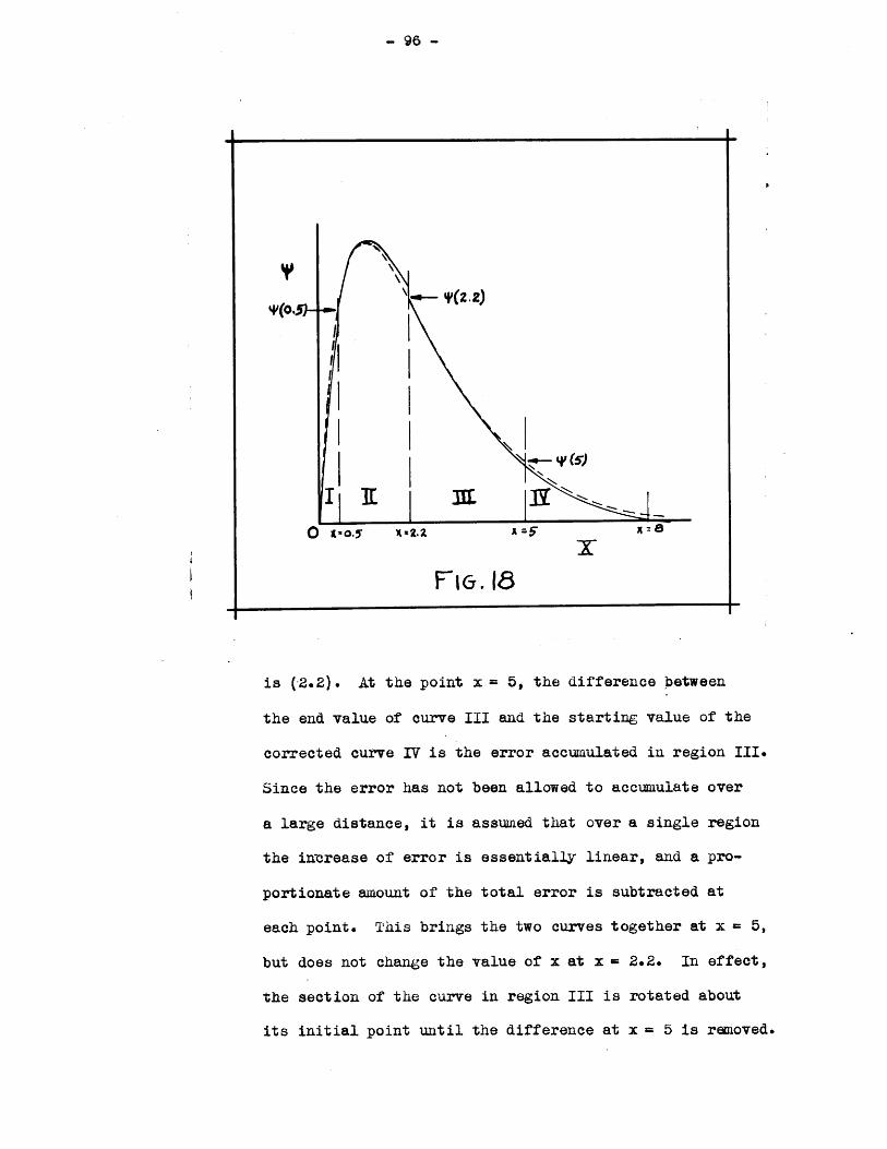
- 96 -
xFie. 18
is (2.2). At the point x = 5, the difference between
the end value of curve III and the starting value of the
corrected curve IV is the error accumulated in region III.
Since the error has not been allowed to accumulate over
a large distance, it is assuned that over a single region
the increase of error is essentially linear, and a pro-
portionate amount of the total error is subtracted at
each point. This brings the two curves together at x = 5,
but does not change the value of x at x = 2.2. In effect,
the section of the curve in region III is rotated about
its initial point until the difference at x = 5 is removed.
.1
4(z.z)
W 3(5)
A Z5"0 '-o.5 x-.2

- 97 -
3. By similar computations make the curve of region II
continuous with that of region III, and likewise finally
make the curve of region I continuous with that of region
II.
4. Repeat steps 1 - 3 for the other set of curves obtained
for the same value of Z.
5. Determine for each curve the value of the integral
J r)2 dx. From x = 0 to x = 5, use Simpson's rule (50
ordinates were used by the writer). From x = 5 to x = "0,
integrate the exponential obtained in step 1.
6. Interpolate between the two curves using the results of
step 5 so that for the final curve -2 dx = 1.
7. From the curve obtained in step 6 find the value of the
integral J 2 _d . This is the constant C in the tem
+ 2. The value of this ten is known from the initial
conditions used; subtracting . from it gives the value
of the energy parameter(.
As a final check on the work, the values of V/are plotted against Z
for various values of x. These curves are shown in Fig. 19. They are
particularly valuable as a check, because the entire procedure is
carried out independently for each value of Z, and the smooth curves
obtained indicate clearly that the procedure is effective in eliminat-
ing accidental error. The only irregularities are in the points for
Z = 6; the wave function for Z = 6 can, as a matter of fact, be read
off more correctly from the curves of Fig. 19 than from the original
data.
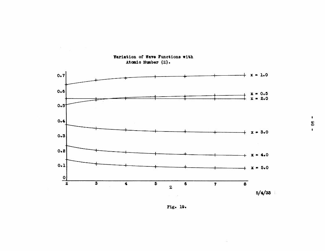
Variation of Wave Functions withAtomio Nmber (Z).
x = 1.0
0*5-
4 x- 3.0
+ x =4.0
0.7
O.4
0.3
0.2
0.1
0
Fig. 19.

- 99 -
Additional computations were made in order to fit thebx dx
empirical equation Y= ax 6 + ex 6 to the final wave fune-
tions*. Using the method of Appendix B, the values of a, b, d and
d were found. The constants were such that one of the texms, say
ax4 6 b , was larger than the other in each case, and became relatively
still larger as either x or Z increased. When "a" and "b" were plotted
against Z, fairly anooth curves were obtained, but "ce" and "d", which
detennined the size of the smaller term,were irregular. In order to
get a consistent set of equations, the "smoothed" values of "a" and
"b" were taken directly from their plots as functions of Z. Then "c"
and "d" were adjusted so that the final equation gave the correct
initial slope and also satisfied the condition dx = 1; the
values of "c" and "d" thus obtained were regular with respect to Z.
The details of these calculations are omitted, but the final equations
are given.
Finally, these empirical expressions for (1 were used to
compute values of to compare with the direct machine results. The
method of computation is given in Appendix C, and the results are in-
cluded in the next section.
f) Results
Calculations of V)were carried out for Z = 2, 3, 4, 5, 6, 7,
8, and 32& The collected results of these calculations are presented
in Tables 2 - 9 inclusive and in Figs. 20 to 27.
* This type of equation for V is one which is frequently used inanalytic studies.

100 -
For each value of Z there are tabulated the numerical values
of I) as a function of x, the empirical equation for . , the value of
derived directly from the machine results, and the value of
computed from the empirical equation. The curve accompanying each
table shows the comparison between the values of Vfrgiven directly by
the machine and the values computed from the enpirical equation.
In Table 10 are grouped for comparison values of as
determined by various computational methodstogether withA,*kp& experi-
mental values. Fig. 28 shows the variation of with Z (Z = 2 to
Z = 8 only).
g) Discussion of method and results
It is interesting to compare the method just described for
obtaining self-consistent solutions, with that which would be required
if the machine were used simply as a means of carrying out the original
Hartree steps. The essential steps for the latter case are listed on
page 70. Having assumed an initial potential field, it is necessary
to solve a linear wave equation and obtain a finite wave function. In
order to control the errors and to adjust the eigenwert, a series of
solutions with varying eigenwert are required, divided into regions
as in the writer's method. From one series of solutions, a single,
finite, continuous wave function is obtained by the method of compu-
tation described in part (e).
Thus far both methods involve the same amount of work. In
the next step of the writer's method, the same process is repeated, and
from these two results, the final wave function can be computed readily.
MArVA-M Q

- 101 -
Table 2
Z W 2 (Hellun)
tV
00.15150.27500.37410.45500.51500.56230.59750.63500.64000.84990.65420.65530.64920.64160.6514
-0. 715xW = 1.012 xE&
-1*50r+ 0.539 xE
0.485 (maachine result)
=1 M 0.408 (camputed)
The following equation fits the above points
better than the first equation listed, but the coef-
ficients do not form part of a smooth curve when
plotted against Z.
V1 = 1.010 x G -0.715X + 0.711 x-&1.499X
x
00.10.20.50.40.50.60.?70.80.91.01.11.21.41.41.5
1.61.71.81.92.02.22.42.62.83.03.54.04.55.0
0.61910.00490.58980.57540.55680.52180.48610.45030.41500.38000.30580.23900.18570.1459
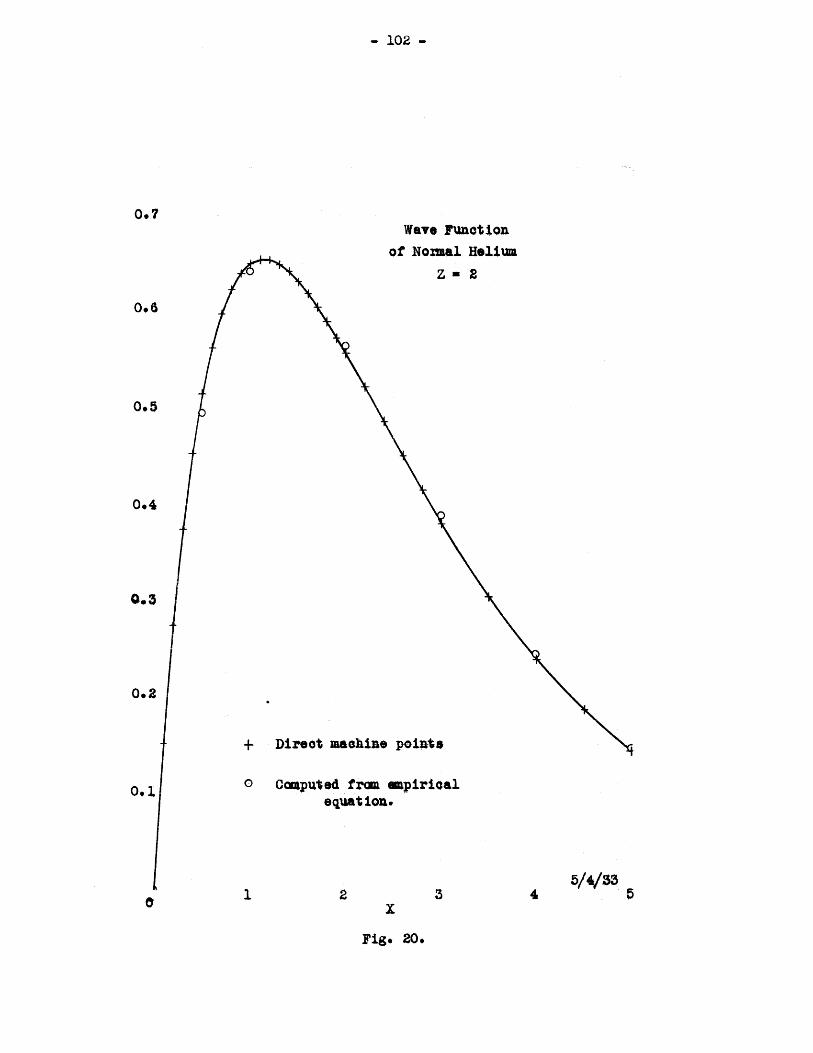
- 102 -
Wave Functionof Nomal Helium
Z w 2
+ Direot machine points
0 Omputed from anpiricalequation.
1 2 3 4
Fig. 20.
0.7
0.6
0.5
0.4
0.3
0.2
0.1
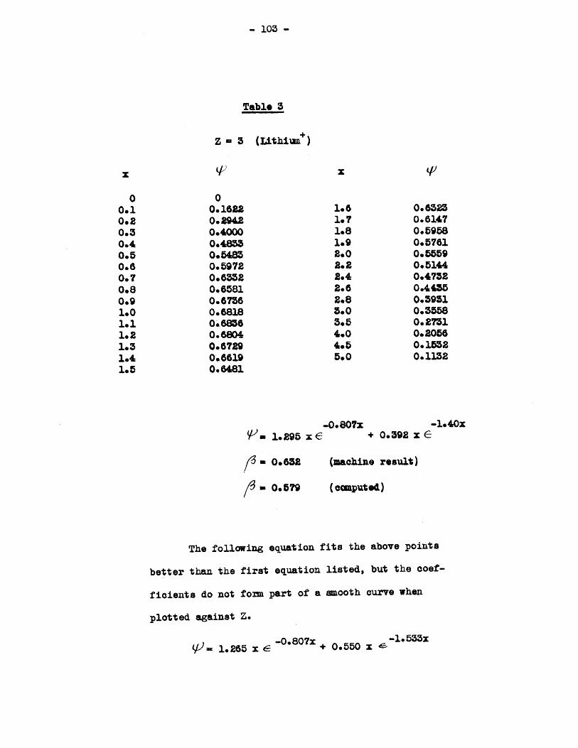
F..Table 3
Z - 3 (Lithiun+
00.16220.29420.40000.48330.548M0.59720.63520.65810.67360.68180A8860.68040.67290.66190.6481
-0.807X -1.40x10 .295 x E- + 0.592 x 6-
= a 0.632
3 - 0.579
(machine result)
(eenputed)
The following equation fits the above points
better than the first equation listed, but the coef-
ficients do not form part of a amooth curve when
plotted against Z.
= 1.265 x C -0.807x + 0.550 x 6-1.555X
- 1o5 -
00.10.20.30.40.50.60.70.80.91.01.11.21.31.41.5
1.61.71.81.92.02.22.42.62.83.03.54.04.55.0
0.63230.61470.59580.57610.55590.510.47320.44350.39310.35580.27510.20560.15320.1132
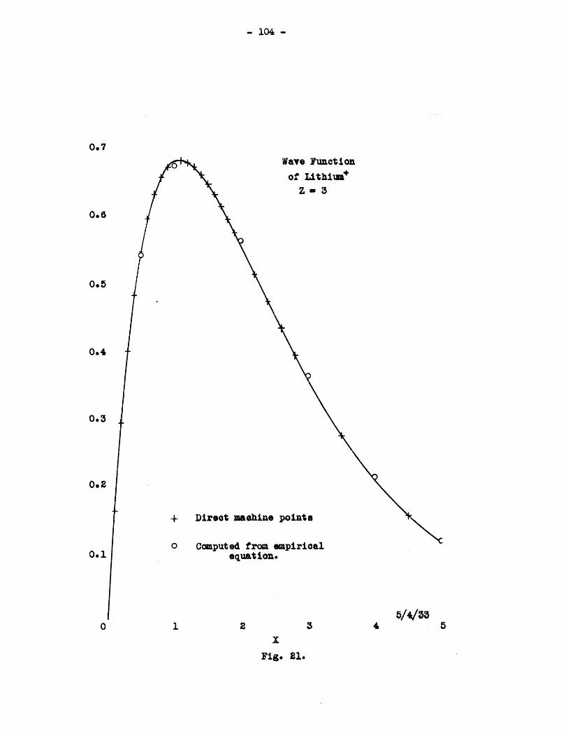
- 104 -
0.7Wave Functionof Lithitaa
Z= 3
0.6
0.5
0.4
0.3
0.2
+ Direct zaahine points
0 Camputed from empirical0.1 equation.
5/4/330 1 2 3 4 5
iFig* 21.
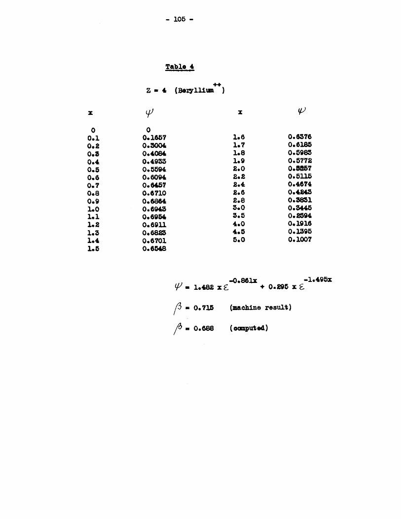
- 105 -
Table 4
Z = 4 (Beryllita
00.16570.50040.40840.49550.55940.60940.64570.67100.68640.69450.69560.69110.68250.67010.6548
= 1.482 X
/ 0.715
/ 0.688
-0.861-xe495+ 0.295 x
(machbine result)
(o4mputed)
x
00.10.20.30.40.50.60.70.80.91.01.11.21.31.41.5
x
1.61.71.81.92.02.22.42.62.8S.03.54.04.55.0
Y-)
0.65760.61850.59850.57720.8570.51150.46740.42450.38510.54450.25940.19160.13950.1007

- 106 -
Waye Funct ionof Bryllian+
Z n 4
Direeot machin points
Computed from empirioalequation.
1 2
Fig. 22.
0.7
0.6
0.5
0.4
0,8
0.1
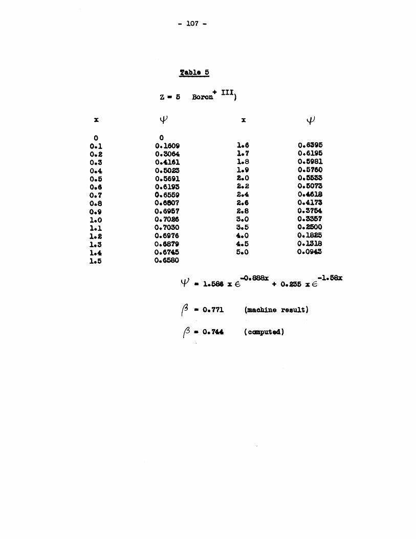
- 107 -
Table 5
Z - 5 Boron 111
0* 16090.30640.41610.50230.56910.61930.65590.68070.69570.70260.70300.69760.68790.67450.6580
x
1.61.71.81.92.02.22.42.62.83.03.54.04.55.0
-0.888X= 1.586 x 6
- 0.771
-1.503+ 0.255 x 6-
(machine result)
3- 0.744 (canputed)
x
00.10.20.30.40.50.60.70.80.91.01.11.21.31.41.5
q)
0.63950.61950.59810.57600.55350.50730.46180.41730.37540.33570.25000.18250.13180.094
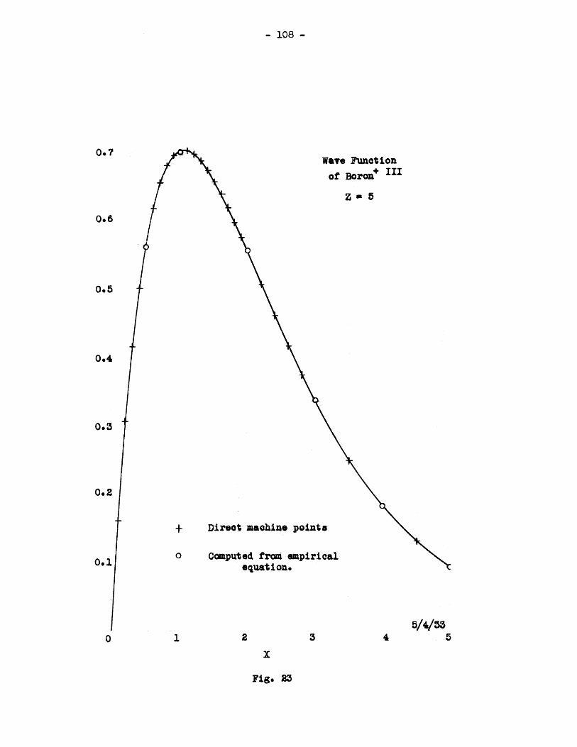
I. ~
- 108 -
Wave Functionof Bron+ II
Z M 5
0.6
0.5
0.4
0.3
0.2
0.1
0 1 2 3 4
Fig* 23
0.7
Direot machine points
Computed froni empiricalequation.
5//33S5
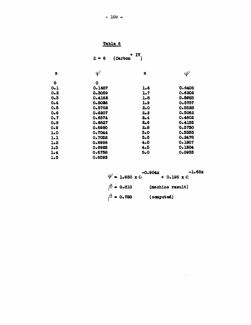
- 109 -
Table 6
+ IVZ = 6 (Carbou )
q0
0.16870.30590.41620.00W0.57020.62070.65740.68270.69800.70440.70520.69960.69230.67580.6593
= 1.650 x 6
{S = 0.810
(3 - 0.788
904x -1.65X+ 0.195 x 6
(machine result)
(ceaputed)
x
00.10.20.30.40.50.60.70.80.91.01.11.21.51.41.5
1.61.71.81.92.02.22.42.62.85.03.54.04.55.0
0.64050.62020.50850.57570.55280.50620.46020.41550.37300.3M50. 24780.18070.13040.0933

r
Wave Funettonof Carbon+ IV
Z a 6
-+ Direct machine points
o Computed from empiricalequatione
1 2
- 110 -
0.7
0.8
0.4
0.3
0.2
5/4/33
Fig. 24.
-I
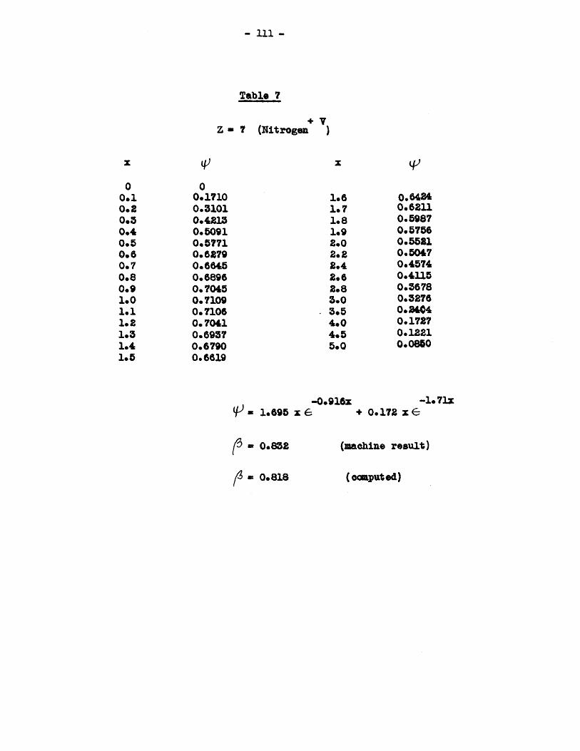
x
00.10.20.30.40.50.60.70.80.91.01.11.21.31.41.5
r
-0.916x= 1.695 x 6
( 0.832
-1.71M+ 0.172 x E
(maechine result)
(ocmputed)
- 111 -
Table 7
Z = 7 (Nitrogen
00.17100.31010.42130.50910.57710.6790.68450.68960.70450.71090.71060.70410.69370.67900.6619
1.61.71.81.92.02.22.42.62.83.0
- 3.54.04.55.0
O.6840.62110.59870.57560.55210*50470.45740.41150.46780.32760.26040.17270.12210.0850
)
= 0.818
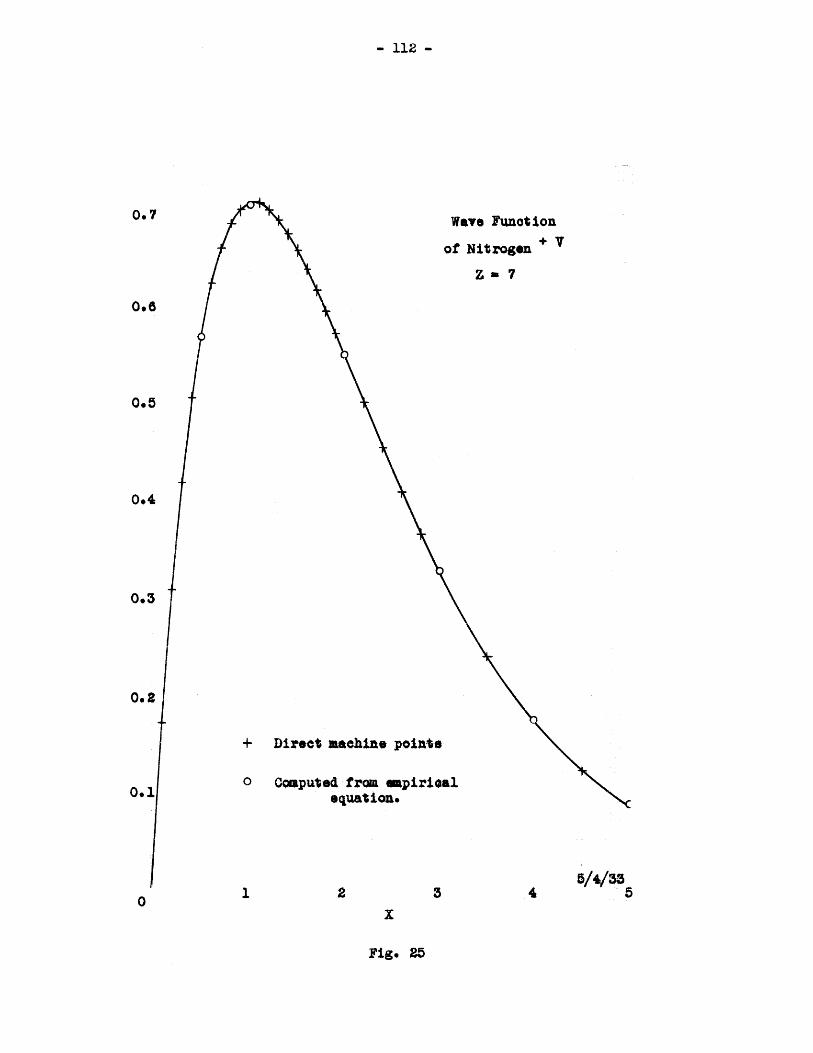
- 112 -
Ways Function
of Nitrogen + V
Z a 7
0.4
0.2
+ Direct machine points
0 0omputed from mpirioalequation.
1 2 3
Fig. 25
0.7
0.6
4
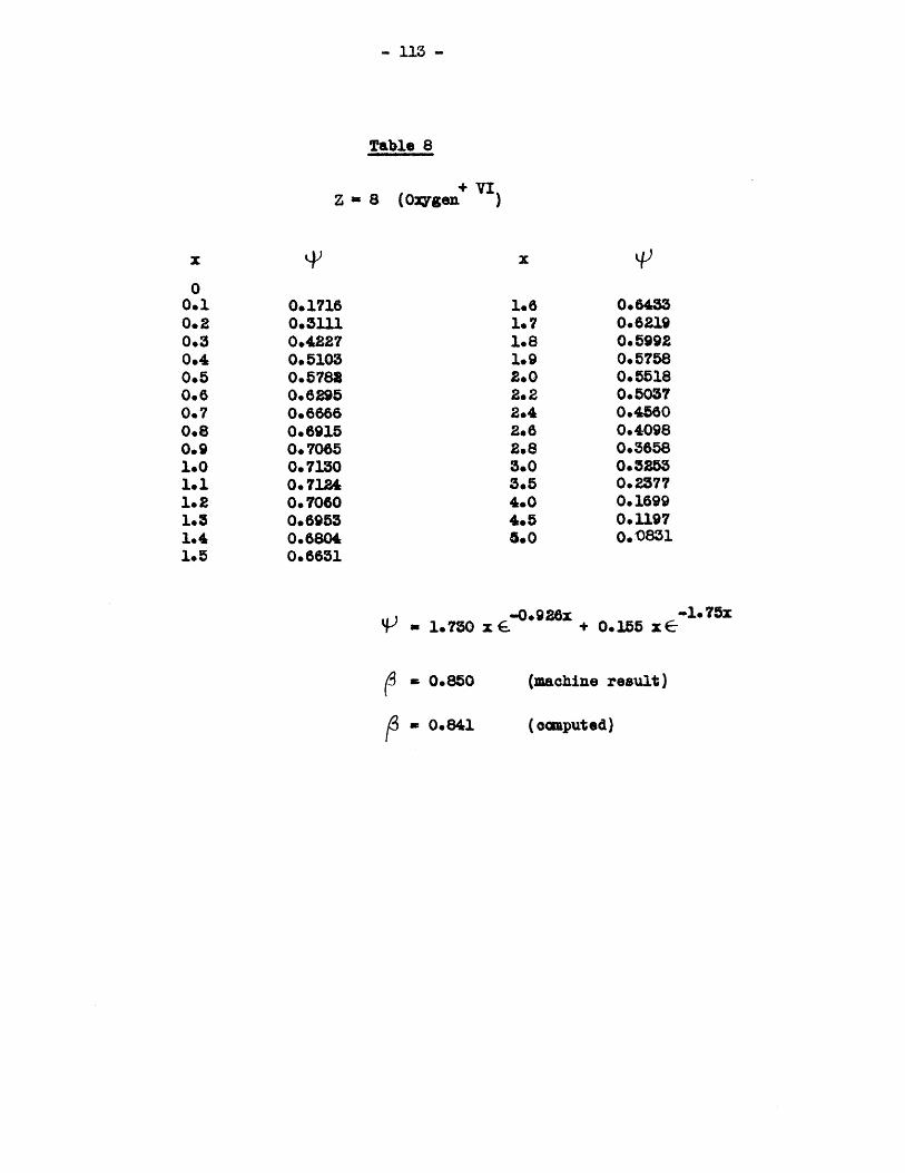
- 113 -
Table 8
+ VIZ = 8 (0:Igen
1.61.71.81.92.02.22.4262.83.03.54.04.55.0
0.64330.62190.59920.57580.55180.50370.45600.40980.36580.32530.23770916990. 11970.0851
-0.926x -l.75xS1.70 x . + 0.155 xEC
(machine result)
(computed)
0.10.20.30.40.50.60.70.80.91.01.11.21.31.41.5
0.17160.31110.42270.51030.57830.82950.66660.69150.70650.71300.71240.70600.69530.68040.6631
= 0.850
= 0.841
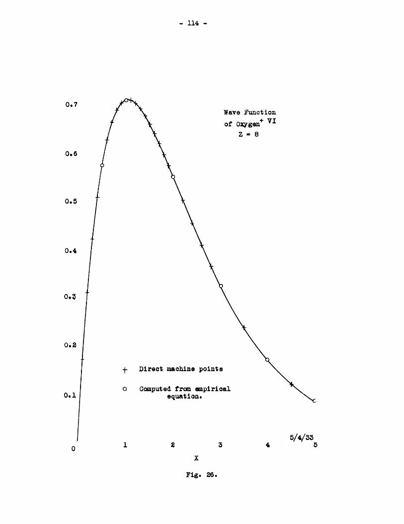
- 114 -
Wave Function
of 0:Qge+ viZ = 8
0.6
0.5
0.4
00Z
0.2
0.1
1 2 3 4
Fig. 26.
0.7
Direct machine points
Computed from empiricalequation.
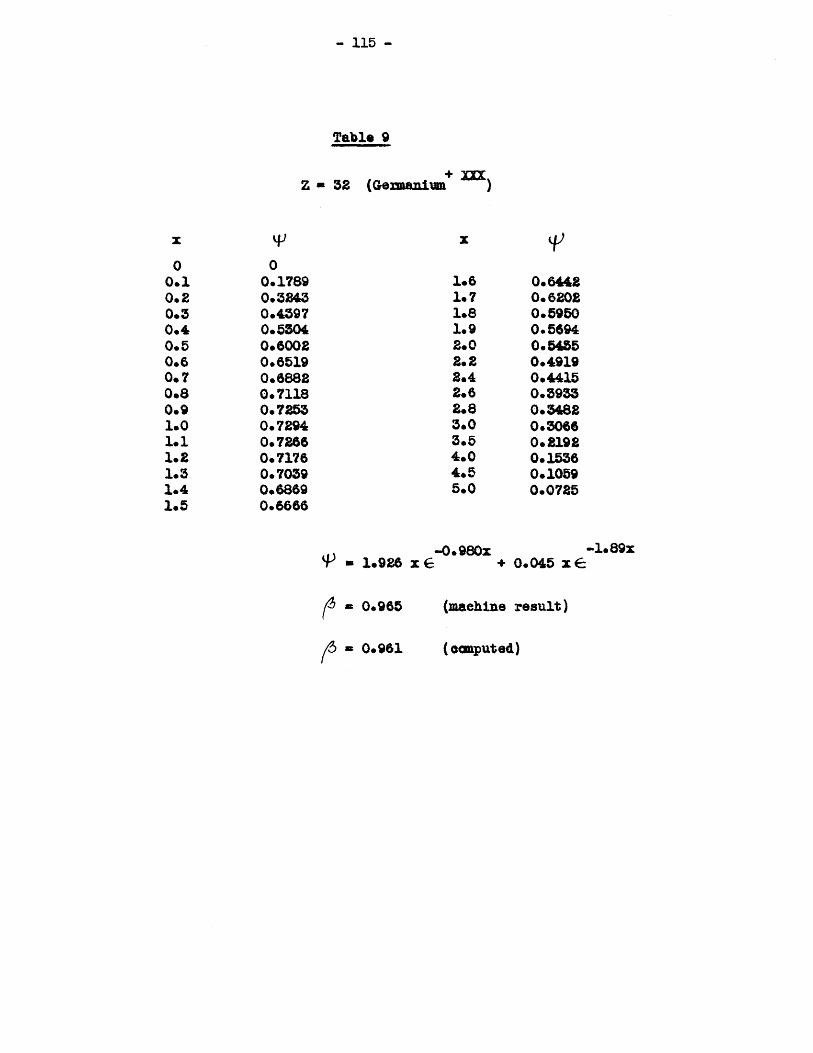
4)
00.17890.32430.43970.53040.60020.65190.68820. 71180.72530.72940.72660.71760.70390.8690.6666
1.61.71.81.92.02.22.42.62.83.03.54.04.55.0
9- 1.926 x6
= 0.965
-0.980x -1e89X+ 0.045 x 6
(machine result)
/3 - 0.961
x
00.10.20.30.40.50.60.70.80.91.01.11.21.31.41.5
0.64420.62020.59500.56940.54550.49190.44150.39330.34820.30660.21920.15360.10590.0725
(onputed)
- 115 -
Table 9
Z = 32 (Gennanium )
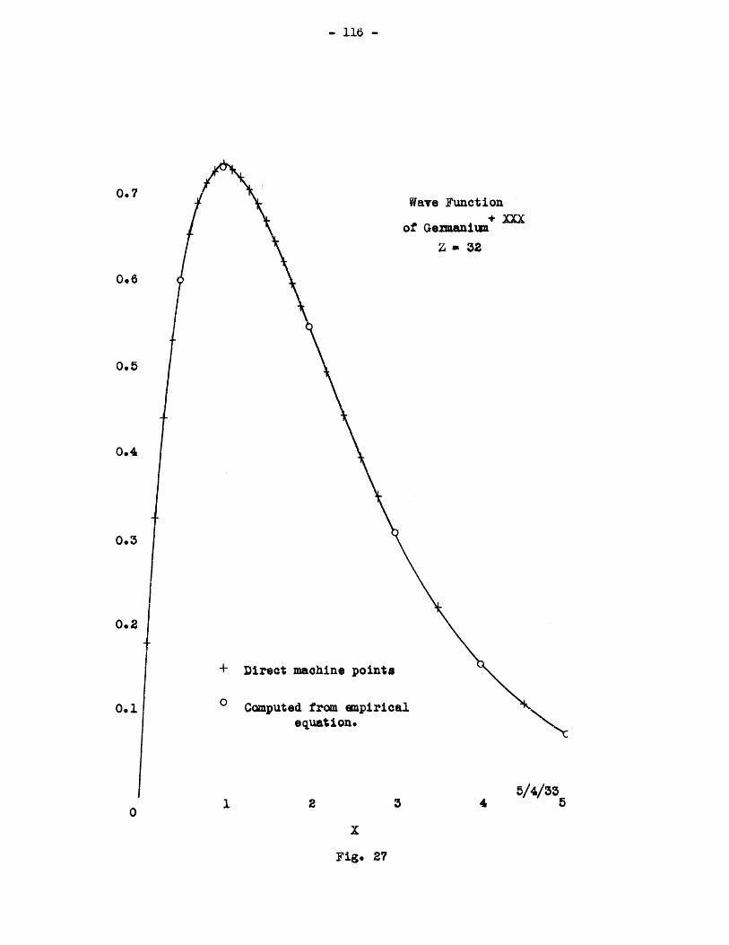
- 116 -
Wave Function
of Grmani+ xxx
Z M 32
+ Direct machine points
0 Computed from eapiricalequation.
1 2 4 5/4/33
Fig. 27
0.7
0.6
0.5
0.4
0.3
0.2
0.1
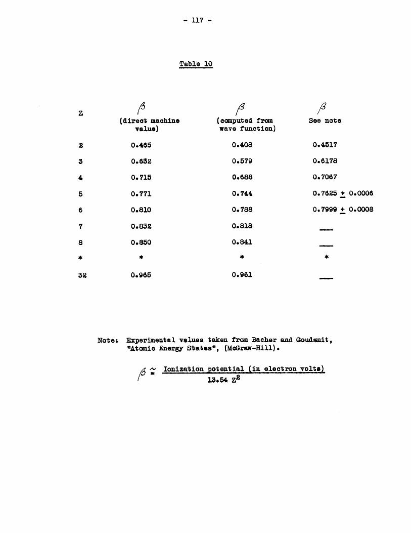
- 117 -
Table 10
(direct machinevalue)
0.465
0. 652
0.715
0.771
0.810
0.852
0.850
*
0.965
/19
(computed fromwave function)
0.408
0.579
0.688
0.744
0.788
0.818
0.841
*
See note
0*4517
0.4178
0.7067
0.7625 + 0.0006
0.7999 + 0.0008
*
0.961
Notes Experimental values taken from Bacher and Goudsmit,"Atomic Energy States", (McGraw-Hill).
Ionization potential (in electron volts)
1.54 Z2
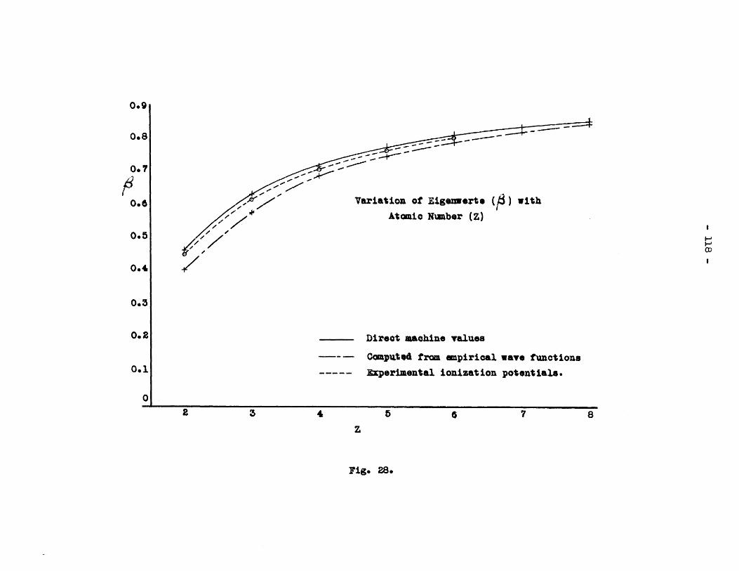
7Variation of Eiguwerte (,3) with
Atomic Number (Z)
7/
Direct aaehine values
---- =OMp140d from empirical wave functions
Experimental ionization potentials.
Fig. 28.
0.8
0.7
0.6
0.5
0.3
0.2
0.1
0
MI
- 119 -
To continue with the Hartree procedure, the wave function just ob-
tained is nomalized, and from it a new potential field is computed
by means of the machine connections of Fig. 11. If this potential
curve is the same as that originally assumed, the calculations are
complete. If not, they must be repeated, as many times as are neces-
sary to obtain correspondence.
In view of the fact that in the writer's method, the extra
step of computing potentials is eliminated, it is apparent that more
operations are required using the Hartree steps if the cycle need
only be gone through twice. Actually, the possibility of assuming
an initial field so nearly correct is rather raote, and in general
the machine operations for the Hartree method will require more time
than is needed for the method described.
From inspection of the wave function curves of Figs. 20 to
27, it is apparent that the points calculated from the empirical equa-
tions derived check the machine points very closely except for Z a 2
and Z = 3. These discrepancies appeared after the numerical coeffi-
cients of all the equations were adjusted as described in the preced-
ing section. As Z decreases, the relative contributions of the two
exponential tenms in the equation for 9 become more nearly of the
same magnitude. The method of adjusting the coefficients, however,
depends for accuracy on having one term considerably larger than
the other. If the curve of each coefficient against Z could be ex-
tended below Z - 2, the results would be improved because the position
of the curve could then be determined more accurately at Z = 2 and
Z = 3. To do this, it would be necessary to obtain the data by solving
- 120 -
the wave equation for, say, Z = 1.5 - a strange atomic configuration,
but merely another gear ratio on the Differential Analyzer.
In both Tables 2 and 3, it will be noted that another empir-
ical equation for the wave function is given; these equations are nor-
malized and fit their respective machine curves, but the coefficients
do not lie on smooth curves when plotted with those of the higher atomic
numbers.
Fig. 28, which gives the variation of the eigenwert with
respect to the atomic nuaber Z shows clearly that consistent results
are obtainable by the method used. The values of obtained directly
from the machine check approximate values computed from experimental
results to within about three per cent at Z = 2 and within nearly one
per cent at Z = 6. (No experimental data are available for higher values
of Z.) These discrepancies between as obtained directly from the
machine and as computed from known ionization potentials are not indica-
tions of error. It so happens that the two results are almost equal
numerically, but the true ionization potential should be computed from
the energy parameter as follows.
The total energy of electron 1 with respect to the nucleus and
electron 2 is equal to 6 Z2 . Likewise the total energy of electron 2
with respect to the nucleus and electron 1 is given by the same value
Z2. If these are added, the total energy of the atom thus obtained
is too large because the mutual energy of the two electrons has been
taken into account twice. It is necessary, therefore, to subtract a
term equal to this mutual energy*. The total energy of the bydrogen-like
* This is obtained as an integral over all space of the form
foi2 v(x)dx, where v(x) is that given by equation (3) of this
chapter. It can be computed from the data presented in Tables2 - 9.

- 121 -
atom which is left after one electron is removed by ionization is
given by Z2. The difference between the total energy of the original
helium-like atom and that of the final hydrogen-like atom is the re-
quired ionization potential (in atomic units). This is given by the
expression
W 2 Z - (mutual energy of the twoelectrons).
This computation is not carried out here because it is not strictly
part of the machine problen of this thesis. All the data required for
the computation are in the tabulated results.
The overall accuracy of machine operation on this problem is
difficult to estimate. In applying the least-square correction to
eliminate the error accunulated in a single region, the maximum correc-
tion of wave function required was about 0.6 per cent while the aver-
age was less than 0.2 per cent. These figures indicate the extent to
which the machine results can be repeated in the presence of cunulative
error. With allowance for systanatic error, the wave functions are
probably accurate to within 0.3 per cent from x = 0 to x = 5. Beyond
this point, the results are less certain. But it should be remembered
that only about 5 per cent of the total charge of the electron is
located in the region beyond x = 5 and hence a 10 per cent error in
ordinates although large on an absolute basis is anall in its effect
on the overall distribution.
- 122 -
Chapter V.
SMLlARY AND CONCLUSIONS
a) Range of application of the present machine
From the camputational methods described and proposed in the
preceding chapters, it is clearly evident that the range of application
of the present Differential Analyzer cannot be defined in terms of the
specific types of ordinary differential equations which it will solve.
The machine is a structure consisting of a limited number of basic units,
usable in whatever sequences and combinations are required. Any state-
ment of its scope must take this important characteristic into account.
Among the various mechanisms contained in the Analyzer, the
integrator is, of course, the most important single unit. At least one
integrator is needed to solve any differential equation, and the limitedd
number of these units is the principal limitation of the present machine.
It is in terms of integrators that the range of application of the mach-
ine must at present be defined.
Now the integrator is a rather versatile mechanism, in a
mathematical sense, especially in combination with others of its kind,
and it is therefore necessary to distinguish in some way between the
operations it perfozms. It is suggested that two types of integrators
be defined, an essential integrator and a functional integrator.
Essential integrators are those which are used only to lower the order
of derivatives; this includes carrying out integrations explicitly
indicated in differential equations, because such equations can be
written without explicit integrals, but in terms of higher order
.. 123 -
derivatives. The functional integrator, used either singly or
in combination with others, performs principally those auxiliary
integrating processes which are not inherent to the problem in hand,
but which are deliberately introduced to gain advantages resulting
ficm automatic operation.
From the definitions given it can be seen that for any prob-
lem the number of essential integrators required is equal to the order
of the equation. This follows from the fact than an nth order deriva-
tive must be put through n integrations in order to obtain the depend-
ent variable as a function of the independent variable, and further,
that the order of a differential equation is by definition equal to
that of the highest order derivative appearing in it. Since the
dependent variable must be produced explicitly, it follows that the
minimum number of integrators required is equal to the order of the
equation. Hence the upper limit of the range of application of the
present Differential Analyzer is the solution of sixth order differ-
ent ial equat ions.
For any particular equation which is to be placed on the
present machine, the number of integrating units available as func-
tional integrators is equal to six minus the order of the equation.
It would be an undue restriction to set up rules in general for the
use of these available functional integrators. As a matter of
experience, however, it has been found that for certain processes,
integrators should be used rather than input tables or multipliers,
and in considering the disposition of available functional integrators,
they should be assigned first to such processes. As an example,
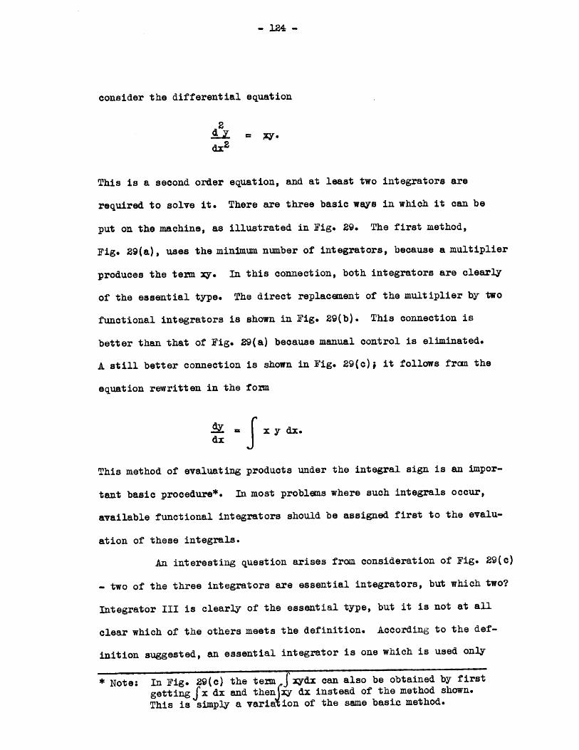
consider the differential equation
2dy = Xzy.
dx 2
This is a second order equation, and at least two integrators are
required to solve it. There are three basic ways in which it can be
put on the machine, as illustrated in Fig. 29. The first method,
Fig. 29(a), uses the minimum number of integrators, because a multiplier
produces the term xy. In this connection, both integrators are clearly
of the essential type. The direct replacement of the multiplier by two
functional integrators is shown in Fig. 29(b). This connection is
better than that of Fig. 29(a) because manual control is eliminated.
A still better connection is shown in Fig. 29(c); it follows frcm the
equation rewritten in the form
x y dx.dx
This method of evaluating products under the integral sign is an impor-
tant basic procedure*. In most problems where such integrals occur,
available functional integrators should be assigned first to the evalu-
ation of these integrals.
An interesting question arises from consideration of Fig. 29(c)
- two of the three integrators are essential integrators, but which two?
Integrator III is clearly of the essential type, but it is not at all
clear which of the others meets the definition. According to the def-
inition suggested, an essential integrator is one which is used only
* Note: In Fig. 29(c) the term Jxydx can also be obtained by first
getting fx dx and then fy dx instead of the method shown.This is simply a varia ion of the same basin method.
Y
(a')
--- - - - -
- - - - - -
- - - - - - - - -
It.(i,)
- -
- - -
--- - - -
I lit(c)
Fi&. Z9
d
X
XYSx
xz
4y x
sxcyjx
-k dlwmdffffdw== q

- 126 -
to lower the order of a derivative. Neither integrator I nor inte-
grator II do this explicitly, but integrator II produces the .Adx
term finally, and by liberal interpretation may be designated as an
essential integrator. Still further trouble is encountered, however,
in certain cases which arise where a derivative is ultimately produced
as a sum of other tems. If the derivative thus produced is of the
same order as the equation, then it will be reduced by a series of
essential integrators. But it frequently happens that it is more con-
venient to produce a lower order derivative as a sum of other terms,
and in such cases it is impossible to distinguish all of the essential
integrators. The point to be made is that although theoretically a
problem can be set up on the Analyzer so that the essential integrators
can be clearly designated, the principal object of classification of
this sort is to aid in defining minimum requirements and maximum range.
Without going further into the details of how to design mach-
ine connections, the following list shows in order of importance and
utility the uses to which available functional integrators should be put.
1. Evaluation of products under the integral sign.
2. Production of simple functions such as squares and exponen-
tials where one integrator replaces one manual operator.
3. Multiplication by use of the rule uv = u dv +J v du
4. Production of general functions. In choosing which func-
tions to produce by integrators, the first object should
be to replace a manual operation by as few integrators as
possible. If the choice on this basis is immaterial, then
design for optimum mechanical performance. For example,

127 -
if two integrators are available to produce either a
sine function or a reciprocal, use them to produce the
sine.
5. Integrators may be used instead of change gears for fine
control of adjustable parameters.
The order given above need not, of course, be followed rigor-
ously if any advantage is obtainable by departing from it. In certain
cases, for example, the order of items 3 and 4 might well be reversed
to advantage- this depends on the requirements of the specific problem.
As illustrated by the very simple example of Fig. 29, there
is great flexibility in the use of integrators for functional purposes.
The maximum range of the machine from the standpoint of essential inte-
grating processes has been stated, but it is doubtful whether a categor-
ical statement of the allowable complexity of an equation can be given.
b) Desirable additions to present equipment
As was mentioned in the preceding section, the principal
limitation on the use of the present Differential Analyzek is in the
restricted number of integrators available. When this machine was
first built, six integrators were considered adequate to handle prac-
tically all the demands which would be made on the machine for some
time to come. Within two months of the time the machine was put into
service, problems arose in which additional integrators could haVe been
used to advantage.
Besides the specific uses of functional integrators which
have been mentioned, certain general advantages accrue from having a

- 128
more adequate supply of these units. The introduction of functional
relations automatically is not only more convenient, but also greater
speed and improved accuracy are thereby obtainable. A machine contain-
ing sufficient integrators can, if desired, be divided and used for two
problems simultaneously, and still be available as a whole. Furtheimore,
the necessity for repair of the units is obvious, and with present operat-
ing schedules it is very difficult to maintain the units properly; even
a single spare integrator would take care of this situation nicely.
The number of additional integrating units which can be in-
stalled to advantage on the present machine is to some extent controlled
by the physical difficulties of getting them in without rebuilding too
much of the machine. By adding one more bay of special design at the
end of the machine now occupied by the recording counter, four addi-
tional integrators can be installed. In addition, the output table can
be shifted to one of the input table positions and the space it now uses
can hold two more integrators. The output table would, of course, be
modified so that it would serve as either an input or an output table
in its new location. The six integrators which could thus be added
would double the present capacity of the machine in this respect and
would greatly increase its utility, speed and accuracy.
At the present time, an investigation is going forward on
methods of following plotted curves automatically*. The results ob-
tained at the present writing are encouraging, and it appears that it
will be feasible in the near future to introduce this refinement on
the machine. There are several reasons why this is a desirable step.
* This investigation is being carried on by Mr. H. A. Traver as anS.M. thesis.

- 129 -
In the first place, no matter how many integrators within reason there
are available, it is almost certain that problems will arise for which
the number of integrators is inadequate, and input plots will have to
be used. For some types of experimental curves, the integrator connec-
tions required to produce them are entirely too complicated. There
are also certain analytic functions which are more satisfactorily intro-
duced from plots than from integrators. In all these cases, it is usu-
ally advantageous to be able to follow the plots automatically, because
of the higher speed and improved accuracy which are available. The
hand control must be retained, of course, for use with certain types of
plots where automatic following is not feasible (e.g. vacuum tube char-
acteristics).
c) Significance of the Differential Analyzer method
The Differential Analyzer method must be regarded in the last
analysis as simply another method of computing certain results. It is
unique, however, in that it combines the power of numerical integration
to handle analytically wmanageable terms and combinations, with the
exactness of analytic solution, which is unattainable numerically except
at the expense of unreasonable labor. Although it is in itself a power-
ful method, it must be supplemented by skill and thorough understanding
on the parts of the men who use it. The hunman brain must plan the
attack in every problem, using such mathematical devices as are neces-
sary and available to produce a workable procedure. In the preceding
chapters a number of examples have been given which show both the gen-
eraL application of the method and the extent to which the basic method

- 130 -
can be modified in order to overcome limitations of equi;ment.
There is more to the Differential Analyzer than merely
setting up a machine and operating it so as to obtain solutions of a
differential equation. No achievement can be claimed for using muscles
instead of nerve tissue to solve mathematical problems. The true aim
of the method is to let the machine do all the work and to reduce even
supervision to a minimum. This has a direct bearing on the one serious
limitation of the method. It has been pointed out that the machine can
anly produce individual solutions of a given equation. In many cases
it is possible by applying methods of generalization to make one of
these single solutions mean more than the answer to a single part of
the problem. Even then, a great many solutions are required in order
to complete an adequate study of the equation over the range of vari-
ables which is of interest. Anything which speeds up the process of
obtaining a solution is a step toward the removal of the limitation
expressed above. Much can be accomplished in this respect by the
complete mechanization of all operations, and there is every hope that
this objective will be realized in the not-too-distant future (see foot-
note page %).
In addition to its primary role as a computing method, there
is some indication that the machine method may be of aid to analysis.
As an example, the consolidation of the Hartree steps made by the writer
was effected because of previous knowledge of the possibilities of the
machine method. The question was not how to solve a given problem on
the machine, but how to express certain physical and mathematical condi-
tions so that the given machine could be used more effectively. In
U
- 131 -
other problems, certain generalizations have been suggested by
peculiarities in the behavior of the machine. Further developments
of this type will undoubtedly appear as the work on the machine pro-
ceeds.
d) Utility and significance of the work in atomic physics
It has been demonstrated that the machine method is directly
applicable to problems of atomic structure in the stationary state.
The method finally developed is straightforward and with care and
systematic operation will produce the desired results in a reasonable
length of time. Working with one assistant, the writer was finally
able to carry out in less than twelve hours all machine operations
and associated least-square camputations necessary to solve for a
single wave function (one atom). This time was possible, of course,
only after the machine had been set up and after the necessary pro-
cedures had been established. If a series of wave functions is to
be obtained (which is usually the case) it can be maintained as a
steady pace. A unique feature of the procedure is the method used
to control the cumulative error due to accidental inaccuracies of
operation.
Eight wave functions are presented both numerically and
with corresponding empirical formulas. These results have already
been applied in further work and are applicable to other studies in
atomic physics. As brought out in Chapter 17, the energy values given
are first approximations to the ionization potentials. Further inte-
grations are necessary in order to campute the corrections applicable
to these values.
-132-
The theory of atomic structure, as expressed in quantum
mechanics, has undergone revolutionary change and phenomenal develop-
ment in very recent years. It has attained a unity of construction
which permits direct application of basis principles in the writing
of the wave equations for given states, and in the interpretation of
the solutions of these equations in physical and chemical terms. But
the gap between the wave equation and its solutions is still large,
even in relatively simple cases. The success which has thus far
attended the effort to close this gap by means of the Differential
Analyzer is encouraging; this machine and its projected improvements
offer to atomic physics unique procedures for further advance, by
removing computation barriers which now stand in the way.
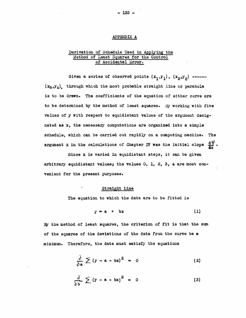
- 133 -
APPENDIX A
Derivation of Schedule Used in Applying theMethod of Least Squares for the Control
of Accidental Error.
Given a series of observed points (x 1,Yi), '2t2)*------
(Xn,yn), through which the most probable straight line or parabola
is to be drawn. The coefficients of the equation of either curve are
to be determined by the method of least squares. By working with five
values of y with respect to equidistant values of the argument desig-
nated as x, the necessary computations are organized into a simple
schedule, which can be carried out rapidly on a computing machine. The
argument x in the calculations of Chapter IV was the initial slope AT.ax
Since x is varied in equidistant steps, it can be given
arbitrary equidistant values; the values 0, 1, 2, 3, 4 are most con-
venient for the present purposes.
Straight Line
The equation to which the data are to be fitted is
y a + bx (1)
Br the method of least squares, the criterion of fit is that the sum
of the squares of the deviations of the data from the curve be a
minimum. Therefore, the data must satisfy the equations
2 j(y - a -bx)2 0 (2)
(y - a - bx) 0 (3)Sbb
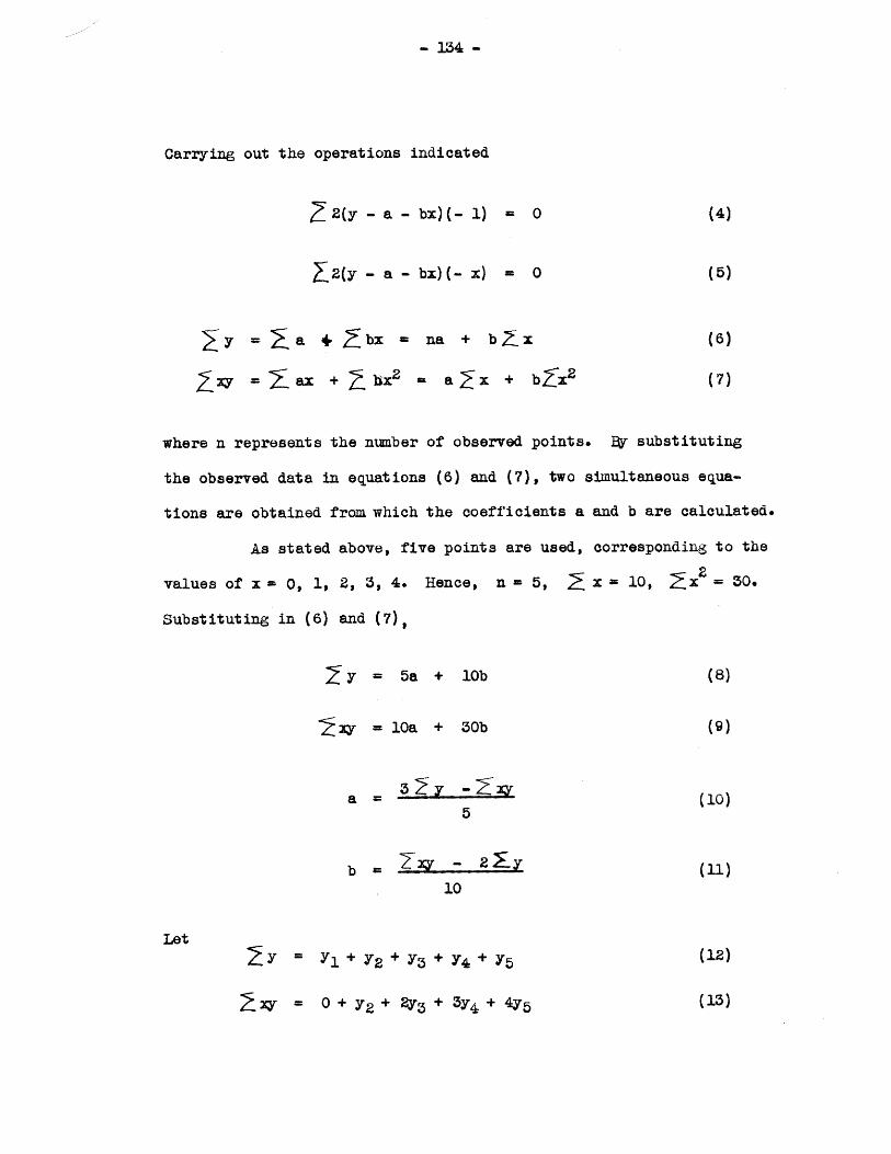
Carrying out the operations indicated
72(y - a - bx)(- 1) = 0 (4)
L2(y - a - bx)(- x) = 0 (5)
y = a + bx na + b 7 x (6)
xy = 2 ax + tjx 2 a 2 x + bfx 2 (7)
where n represents the number of observed points. By substituting
the observed data in equations (6) and (7), two simultaneous equa-
tions are obtained from which the coefficients a and b are calculated.
As stated above, five points are used, corresponding to the
values of x = 0, 1, 2, 3, 4. Hence, n W 5, x 10, 2x = 30.
Substituting in (6) and (7),
2 y = 5a + 10b (8)
xiy = 10a + 30b (9)
3 y - (10)5
b -2217 (11)10
Lety= yl + y2 + y 3 + y4 + y 5 (12)
2 xy = 0 + y 2 + 2y 3 + 3y4 + 4y5 (13)
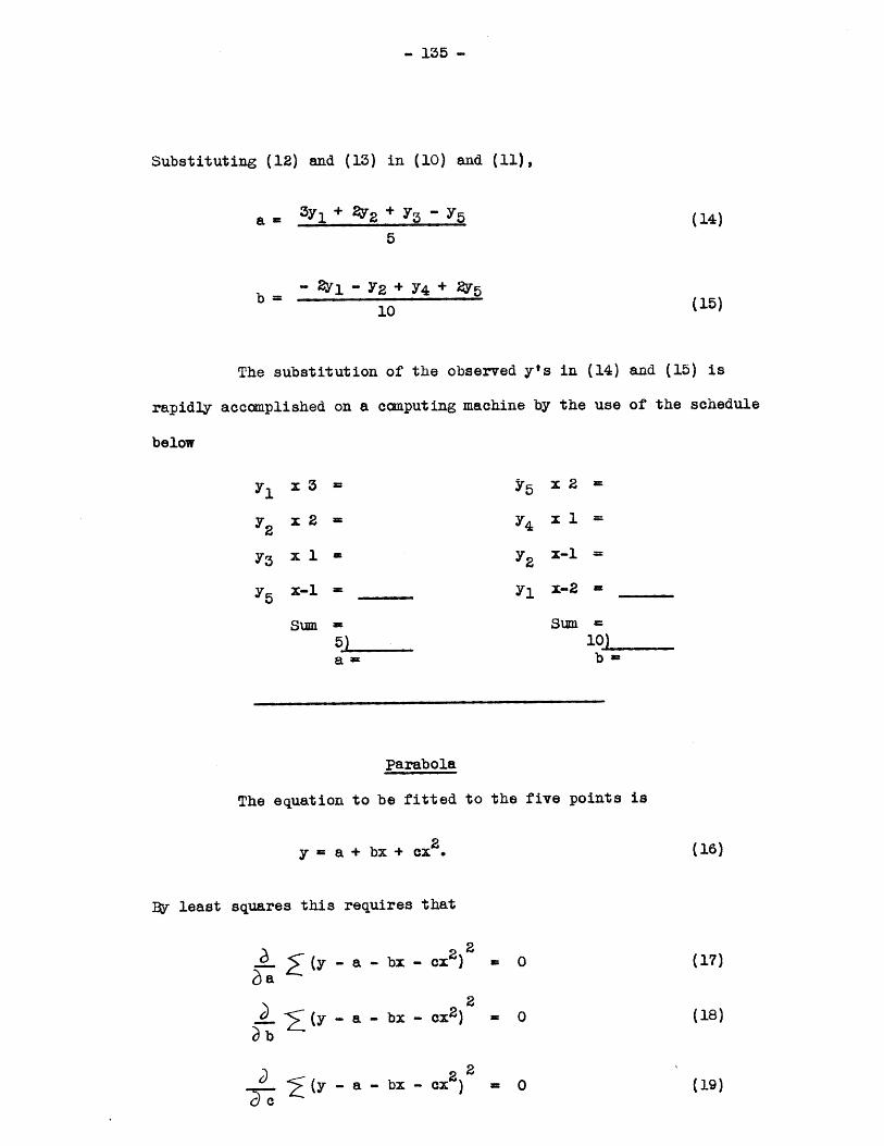
- 135 -
Substituting (12) and (13) in (10) and (11),
a = 3y + 2y+y 3 5
- 2yl - Y2 + Y4 + 45(15)
The substitution of the observed y's
rapidly accomplished on a computing machine by
below
x 3
x 2
x 1
x-l
Sum
in (14) and (15) is
the use of the schedule
xl2
x-1
x-2
Sun=
5)a
10)
b=
Parabola
The equation to be fitted to the five points is
y = a + bx + ex2
By least squares this requires that
_~2
3 ;(y - a - bx - cx2)2ha
2(y - a - bx - cx2)
Sb
0 (y - a - bx - ex2 2
=0
=0
(17)
(18)
= 0 (
(14)
(16)
(19)
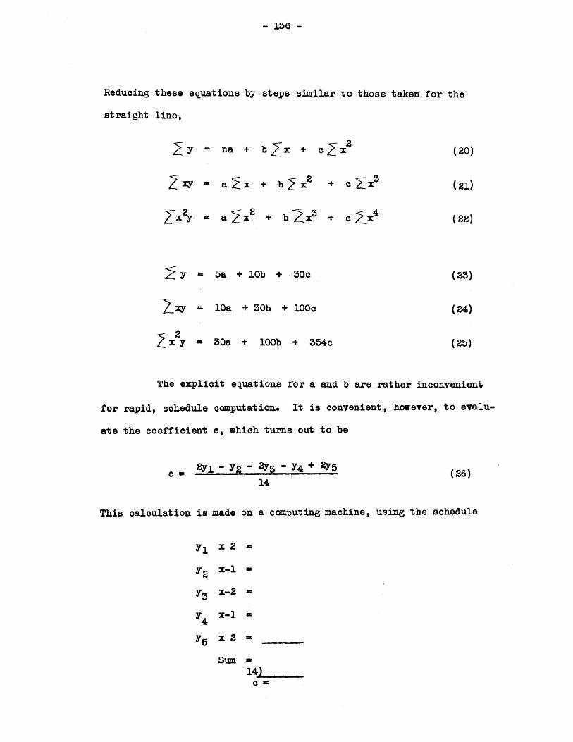
Z 37 = a 2 x + b x 2 +
xy = a 2x 2 + b 2x3 +
O .3
O x
(21)
(22)
(23)
(24)
(25)
y .5a + 10b + 30c
Zxy =10a + 30b + 100c
x y= 30a + 100b + 354c
The explicit equations for a and b are rather inconvenient
for rapid, schedule camputation. It is convenient, however, to evalu-
ate the coefficient C, which turns out to be
0 2yy 2 - 2 -Y 4 + 2Y5 (26)14
This calculation is made on a computing machine, using the schedule
y1
Y2
y3
yY4
y5
x 2
X-1
x-2
x-l
x 2
Sum
- 136 -
Reducing these equations by steps similar to those taken for the
straight line,
2 y = na + b jx + cZx2 (20)

- 137 -
2Khowing c, the value of cx at each point can be determined, and
when subtracted from the original parabolic data, the result is a
series of points which can be represented by a straight line. Thus
Y2 = Y2 - c
Y73 = Y3 - 4a
Y4 = Y4 - 90
Y-5 = Y5 - 16c
The equation of the straight line through the y data is obtained
using the schedule on page /5
- 138 -
APPENDIX B
Method of Fitting Bapirical Wave Functions
to the Machine Data
The equation to which the data is fitted is
4 = ax ebx + cx E
This is conveniently handled in the form
ox dxy a C = a + ce6
The constants of equation (2) are found by the following method*.
Consider three successive y-values, y1, y29 y3 , correspond-
ing to the equidistant x-values xl, x, + h, x, + Eh. For these the
equations are written
abx, dx,y aa6 + cOE
Y2 - a b(xl+h) d(xl+h)
+ d(xi+2h)y3 = a E b(xi+2h)
(3)
bx bha aE Ce + cE E
bxil 2bh= aE G
(4)
dxl 2dh+ ce r-
(5)
Multiplying equation (3) by C(b+d)h and equation (4) by -(&bh + dh
and adding these products to equation (5),
y ( bh + 6dh y2 + (2+ b+d)h yi 0 (6)
* Lipka, "Graphical and Mechanical Computation", p. 156.
(1)
(2)
- 139 -
bhor Y_3.= ( E
71
dh y2 (b+d)h+ ).Y. -
Yjl(7)
bh dh (b+d)hSubstituting A ( + 6 ), and B =
the equation for any set of successive values of y is written
Yn+2 P.A- n
Yn(8)
This is the equation of a straight line in yn+2
and from it the exponential coefficients b and d
Eiowing b and d, the original equation
Y 6 = aE +0
and t ,
are determined.
(2) is rewritten
(9)
This equation is linear in y 6 and O(b-d)x, and frcm it the coef-
ficients a and a are determined.
Although the coefficients of the original equation could be
detemnined directly by least squares, the process is very ccmplicated
and requires entirely too much time. The same results are achieved
by using the method described above, and fitting straight lines to
equations (8) and (9) by the method of least squares. This method was
used in the present work and was found to be very satisfactory.
- 140-
APPENDIX C
Calculation of E;nergy Parameter from the
Equat ion of the Wave Function
The wave equation which was solved is
d~(- + -0. + 2 2dx - ) / (i)dxdx 2 ZJX
O
where C .jxi . If the terms of equation (1) are rearranged soJx
as to solve for , and the expression
axbx dxaxE + ex6 (2)
is substituted, it can be shown that varies from an infinite value
at x =0 to a zero value at x = 00 . The desired value of 0 is the
most probable value, and this found by using the wave function as a
weighting function and integrating over all space. Accordingly, the
expression to be evaluated is
010
The reduction of this integral in terms of the coefficients
of the wave function (2) is 'rather involved, and will be omitted since
it consists merely of algebraic substitution and integration. The
final expression for as thus calculated, is given below.

- 141 -
( + 4abcd + )
- .+
64Z b5 d5
+ (1- )(a 2 + 2 + 2
a2.2 1 + b + 5 + i + dz 23 (~) d
8acZ(b+d) 2
a2 (1 + 3b + d)
(3b + d)3
ao a2 5b+ dZ (3b+d) b
+ 02(l + b + 3d)(b + 3d) 3 J
+ 2 b+ 5d
(b+3d) 3 4d 3
This expression is not particularly siNple to use numer-
ically, but the calculated value of thus obtained is useful as a
check against gross error in the wave function.
73
- 142 -
APPENDIX D
Calculation of Scale Factors
For the problem of the self-consistent field using the equation
dq) + 2C+A 2(q2 -x ((-)] qd.dx
dx JJ) Z ZJJ
F J) dFx - 2 dx,
the machine connections with gear ratios indicated are shown in Fig. 30.
It will be observed that un1mown gear ratios are indicated at all points
where the driven shaft is connected directly to a shaft of limited dis-
placement. Furthermore, gear ratios are inserted in drives to differ-
ential gears (adders) in order to permit equalization of scale factors
at these points.
In assigning the scale factors to the various shafts, it is
customary to start with the shaft representing the independent variable.
This shaft is labelled Ax in this case, meaning that the shaft rotates
"A" turns for every unit of "x", and its displacement at any instant is
hence the product Ax. Since this shaft drives the abscissa lead screw
of the input table, which has a maximum allowable displacement of 480
turns, it is stepped down by the gear ratio nl. The ordinate scale of
the plot is unknown, hence the scale factor "B" is assigned to the
shaft; the maximunm allowable displacement of the ordinate lead screw is
360 turns. For the q)- shaft, another unknown scale factor "C" is
assigned as shown. All remaining scale factors can be computed from
those now assigned, making use of the fact that the scale factor of the
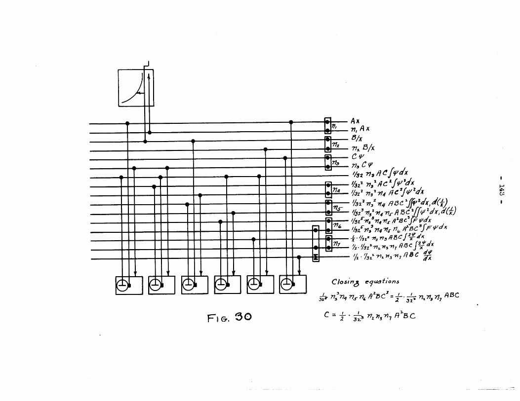
Fi&. SO
Ax
s , n ,lA1I'f ,2'x
Sznj A ~
j n/2 n,'-4 1A5/X
1±2 /j |1,iin e~~Tc ffyi 2d, d()
n*./tn1,ncf~'d-- , . nC nsnc fdx
C losine e 1 BJtionls
,fn~~nq/ _c=_ynn~iAC
c=t- +? ".0 7 sc
milk.
-- - I I I I I
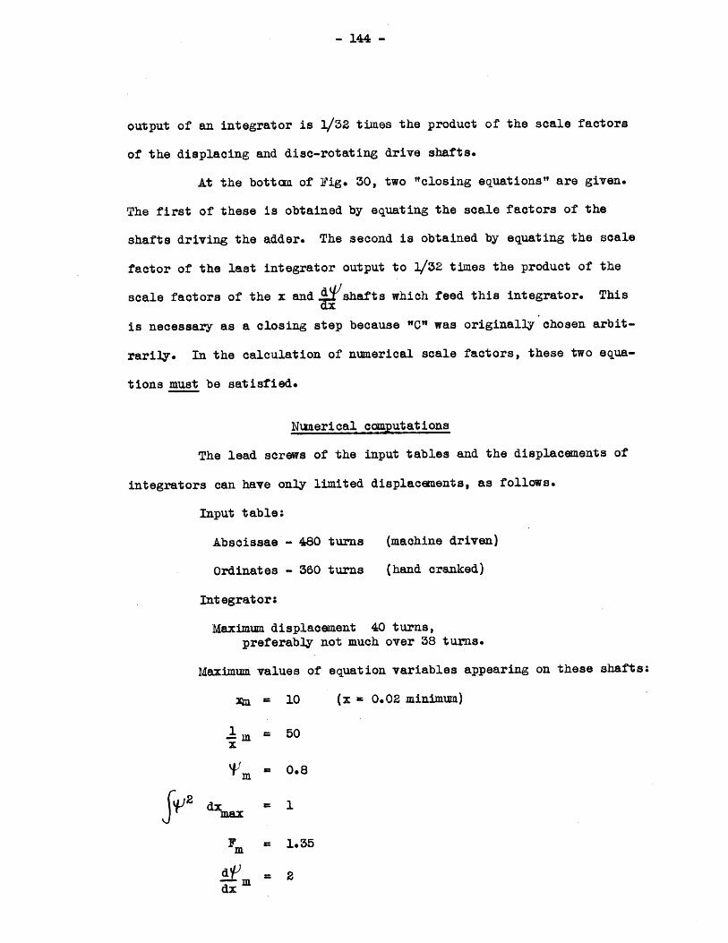
10.1
- 144 -
output of an integrator is 1/32 times the product of the scale factors
of the displacing and disc-rotating drive shafts.
At the bottan of Fig. 30, two "closing equations" are given.
The first of these is obtained by equating the scale factors of the
shafts driving the adder. The second is obtained by equating the scale
factor of the last integrator output to 1/32 times the product of the
scale factors of the x and dt/shafts which feed this integrator. This
is necessary as a closing step because "C" was originally chosen arbit-
rarily. In the calculation of numerical scale factors, these two equa-
tions must be satisfied.
Numerical computations
The lead screws of the input tables and the displacements of
integrators can have only limited displacements, as follows.
Input table:
Abscissae - 480 turns (machine driven)
Ordinates - 360 turns (hand cranked)
Integrator*
Maximum displacement 40 turns,preferably not much over 38 turns.
Maximum values of equation variables appearing on these shafts;
An 10 (x 0.02 minimua)
m 50
fr~d7m =10.
2
Fm 1.35
dxm
- -5.0 W__ _ __ - mommillea -aW.Migm- -I
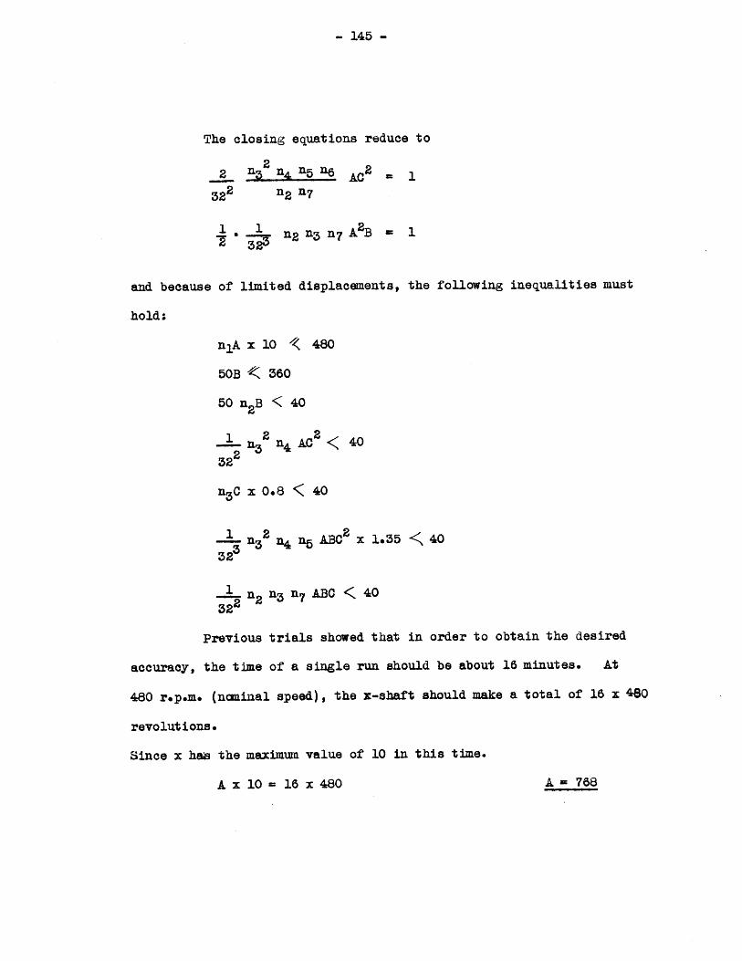
- 145 -
The closing equations reduce to
22 n3 n45 "6 AC2 1
322 n2 n7
. n 2 n3 n7 A2 B = 1
and because of limited displacements, the following inequalities must
hold:
n1 A x 10 'K 480
50B < 360
50 n2B C 40
1 2 2 4n3 n4 AC 40
32
n3C x 0. 8 < 40
1 2- .- 3 n4 6 ABC2 x 1.35 40
323
n2 n3 n7 ABC < 40322
Previous trials showed that in order to obtain the desired
accuracy, the time of a single run should be about 16 minutes. At
480 r.p.m. (noninal speed), the x-shaft should make a total of 16 x 480
revolutions.
Since x has the maximum value of 10 in this time.
A x 10 = 16 x 480 A 768
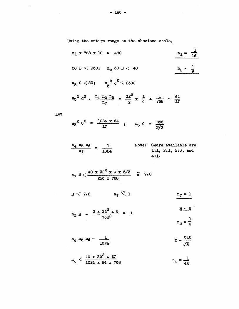
- 146 -
Using the entire range on the abscissa scale,
ni x 768 x 10 a 480
50 B < 360; n 2 50 B < 40
n 2 C < 2500
n32 2 , n4 n5 En6 .
n7
323
2
11-
91 . 64
768 27
n32 2 1024 x 64
27U3 C = 256
Note; Gears available are1:1, 2:1, 2:3, and4:1.
B 40
B < 7.2
x 322 x 9 x 3/3256 x 768
n7 7 1
2 x 32 x 93 7682
114 n5 n6
4
=.1
1
1024
40 x 322 x 271024 x 64 x 768
113 C (50;
n =
n2*
Let
A4 n5 n6117 1024
2' 9.8
n7 = 1
B 6
C
14 1148

- 147 -
n5 n6o 64
340 x 32 x 27 x 48
1.35 x 1024 x 64 x 768n5I
n6 -
A = 768
B= 6
S512
Sunmary
nj = 1
n2 =
n3=
n = 1
48
.5 = 1
n6~ * 64
n7 = 1
Using these scale factors, the physical set-up of the
machine is designed as shown in Fig. 31. On this sheet, the complete
set of shaft constants is also recorded. The necessary gear changes
are indicated also; these must be such that the closing equations are
still satisfied and no displacements are too large.

Sco-nst- A 5CDEFG4 __ x _ XS16 X _X X4 x X X X
6 3Z X X X7 X x x _
81 C X XI_(
32 x _x
Z- GEAit5
C
Lz
* ~~f- xv d()9Jyudx4
L
Oici)iz tij-~Ifl
J.P dx
%.~
tli
fe1
+lf *iC
PL-or 5cAi
L1.- SPEC
G&EA5qs.
./oxcoNTEkR- ,1fp
71
F~/&c.
- - -- - - - - - -z z:41 1-L
-- G S
J I_ -
P --- s
76T I I I I I IE
i
+-ti-
G NOR'IAu /6-imaes '4 iv"y
"M R1:eu 4sIw2 AetILwa#1~t 77:1 E67I
V 4:1 4 : 1 4:1P i:i 4: A:L
R ~~ 1 6:1 60- 4:1 /1
-r /: / 4 : 1:/
A
04
- 149 -
APPE91IX E
Symbola
It is convenient to have standard symbols to represent
the machine units. These sybols have been saployed throughout
this thesis in illustrating methods of dealing with various prob-
lems on the machine. In Fig. 32, the symbols of the most conmon
units are shown.
Of the symbols shown, those of the integrator, multiplier-
divider, input table, and adder appear most frequently; the others
are used only in the physical connection diagram of Fig. 31.

150
V v I
Int egratw m k u
P Q
Input Table
P = f(Q)
Spiral Gear Boxes
(right hand) (left hand)
Spur Gear Set
(ratio shown by figures)
Fig. 32.
- 151 -
BIBLIOGRAPHY
1. Bush, V. The Differential Analyzer. A New Machine for SolvingDifferential Equations, Jour. of the Franklin Inst., Vol. 212,No. 4, October, 1931.
2. Bush, V., Gage, F. D., and Stewart, H. R. A Continuous Integraph,Jour. of the Franklin Inst., January, 1927.
3. Bush, V. and Hazen, H. L. Integraph Solution of Differential Equa-tions, Jour. of the Franklin Inst., November, 1927.
4. Hazen, H. L. The Extension of Electrical Engineering Analysisthrough the Reduction of Computational Limitations by Mechan-ical Methods, Sc.D. Thesis, June, 1931.
5. Kear, F. G., Jr. Integraph Solution of Simultaneous DifferentialEquations, S.M. Thesis, 1928.
6. Kingsley, C., Jr. Calculation of Three-Phase Short-Circuit Currentsof a Synchronous Machine by M1eans of the Differential Analyzer,S.M. Thesis, June, 1932.
7. Edgerton, H. E. Abrupt Change of Load on a Synchronous Machine,S.M. Thesis, 1927.
8. Iyon, W. V. and Edgerton, H. E. Transient Torque-Angle Characteristics,,Presented A.I.E.E. Convention, Jan. 27-31, 1930.
9. Teplow, L. Stability of Synchronous Motors Under Variable TorqueLoads, S.M. Thesis, 1927.
10. Teplow, L. Stability of Synchronous Motors as Determined by the,Recording Product Integraph, G.E. Review, July, 1928. Vol. 31,No. 7, pp. 356 - 365.
11. Church, E. A. and Willcutt, F. W. Improvement of TransientStability of Power Systems, S.M. Thesis, 1928.
12. Tsang, N. F. Surging of Synchronous Motors under Sudden Load,S.M. Thesis, 1928.
13. Cutts, R., Jr. The Effect of Suddenly Applied Load on the Shaftof a Synchronous Motor with a Single Phase Non-Salient PoleRotor, S.M. Thesis, 1928.
14. Vieweger, A. L. Stability of Synchronous Machines under AbruptLoading, S.M. Thesis, 1929.
- 152 -
15. Smith, C. C. An Integraph Analysis of the Sudden Application ofLoad to a Salient-Pole Synchronous Motor, S.M. Thesis, 1929.
16. Hu, J. T. The Torque-Angle Characteristics of a Synchronous Motorunder Pulsating Impressed Load, S.M. Thesis, 1929.
17. Sumers, I. H. and McClure, X. B. Progress in the Study of SystemStability, Jour. A.I.E.E., Vol. 49, p. 132, January, 1930.
18. Gewertz, C. The Pulling-into-Step of a Synchronous Induction(Autosynchronous) Motor, S.M. Thesis, 1928.
19. Zak, F. 5. Synchronizing an Induction Synchronous Machine, S.M.Thesis, 1929.
20. Edgerton, H. E. and Zak, F. J. The Pulling-into-Step of aSynchronous Induction Motor, I.E.E. Jour., Vol. 68, No. 405,September, 1930.
21. Fourmarier, P. The Pulling-into-Step of a Salient-Pole Synchron-ous Motor, S.M. Thesis, 1930.
22. Edgerton, H. E. and Fouxmarier, P. The Pulling-into-Step of aSalient-Pole Synchronous Motor, Presented A.I.E.E., Jan. 26-30,1931.
23. Edgerton, H. E. Benefits of Angularly-Controlled Field Switchingon the Pulling-into-Step Ability of Salient-Pole SynchronousMotors, Sc.D. Thesis, 1931.
24. Brown, G. S. and Germeshausen, K. J. The Effect of ControlledField Switching on the Pulling-into-Step of a SynchronousInduction Motor, S.B. Thesis, 1931.
25. Hamilton, R. W. The Effect of Field Transients on the Pulling-into-Step of Synchronous Induction Motors, S.M. Thesis, 1932.
26. Edgerton, H. E., Brown, G. S., Genueshausen, K. J., and Hamilton,R. W. Synchronous Motor Pulling-into-Step Phenomena, PresentedA.I.E.E., January, 1933.
27. Bachli, W. K. and Chibas, J. E. A Study of a Non-Linear SeriesParallel Circuit, S.M. Thesis, 1932.
28. Smith, T. R. Investigation of the Volt-Ampere Characteristics ofa Non-Linear R.L.C. Series Circuit, S.B. Thesis, 1932.
29. McGraw, X. E. Experimental and Integraph Study of the DynatronOscillator Operating at Low Frequencies, S.M. Thesis, 1932.
- 153 -
30. 11adford, W. H. The Solution of Vacuum Tube Circuit Problems byMeans of the Differential Analyzer, S.M. Thesis, 1932.
31. Bell, 5. S. The solution of the Tuned Grid and the Tuned PlateOscillator Circuits by Means of the Differential Analyzer,S.M. Thesis, 1933.
32. Burnett, C. E. A Study with the Differential Analyzer of theSteady-State and Transient Response of Simple Vacuum-TubeAmplifier Circuits under Different Load Conditions, S.M. Thesis,1933.
33. Fink, D. G. Tentative title - The Prediction of Amplitude ofOscillation in Vacuum-Tube Oscillating Circuits - A Study on theM.I.T. Differential Analyzer, S.B. Thesis, 1933.
34. Gould, K. E. Integration of Functional Product by Measurement ofInfra-Red Radiation, Tour. Opt. Soc. Am. and Rev. Sci. Instr.,pp. 198-206, September, 1928.
35. Gray, T. S. A Photo-Electric Integraph, Jour. Franklin Inst.,Vol. 212, No. 1, July, 1931.
36. Bush, V. and Members of the Research Staff. Transmission LineTransient Investigations, Contr. from Dept. of Elec. Eng.,M.I.T. Serial No. 50, September, 1925.
37. Finley, T. H. and Williams, H. W. Analysis of Three-Phase Trans-mission L4ne Transients, S.M. Thesis, 1926.
38. Hall, W. M. Omments on the Theory of Horns, Jour. Acoustical Soc.Am., Vol. III, No. 4, April, 19321 A Miniature CondenserTransmitter for Sound-Field Measurements, Jour. Acoustical Soc.Am., Vol. IV, No. 1, July, 1932.
39. Guerrieri, X. Methods of Introducing Functional Relations Auto-matically on the Differential Analyzer, S.M. Thesis, 1932.
40. Sears, F. W. Integraph Solutions of Electron Orbits in theBarkhausen-Kurz Effect, Jour. Franklin Inst., 209, pp. 459-472,April, 1930.
41. Lemaitre, G. and Vallarta, M. S. On Compton's Latitude Effect ofCosmic Radiation, Phys. Rev., 43, pp. 87-91, January 15, 1933.
42. St8nmer, Carl. Periodische Elektronenbahnen im Felde einesElementarmagneten und ihre Anwendung auf BrUches Modellversucheund auf Eschenhagens Elementaxwellen des Erdmagnetismus, Zeit.fur Astrophysik, 1, pp. 237-274, 1930.

I KA.
- 154 -
43. Bush, V. and Caldwell, S. H. Thomas-Feimi Equation Solution bythe Differential Analyzer, Phys. Rev., pp. 1898-1902, Vol. 38,No. 10, November 15, 1931.
44. Van Vleck, T. H. Quantum Principles and Line Spectra, Nat. Res.Council Bull. No. 54, 1926.
45. Condon, E. U. and Morse, P. M. Quantum Mechanics. (McGraw-HillBook Co.).
46. Hartree, D. R. The Wave Mechanics of an Atom with a Non-CoulombCentral Field, Proc. Camb.Phil. Soc., 24, pp. 89-132; 426-437;1927-28.
47. Eckart, Carl. The Theory and Calculation of Screening Constants,Pbys. Rev. 36, pp. 878-892 (1930).
- 155 -
BIOGRAPHICAL SKETCH
The writer completed his secondary school work at the
Frankford High School, Philadelphia, Pa., in February, 1921, and
entered the Massachusetts Institute of Technologyin October, 1921.
He registered in Course VI-A at the Institute and took his co-operative
work with the General Electric Co. principally at the LYnn, Mass. plant,
starting in March 1923. Assignments at the General Electric Co. in-
cluded tests on constant-current transfoners, small motors and gener-
ators, and rectifiers at Iynn, and large induction motors at Schenectady.
His thesis research for the Master's degree was carried out in the
Tungar laboratory at Lynn on "Characteristics and Theory of Operation
of a Dry Electrolytic Rectifier". In Tune 1926, he was awarded by the
Institute the degrees of S.B. (as of 1925), and S.M.
In February 1926, he was appointed as an Assistant in the
Electrical Engineering Department and assigned to carry on work in the
cable research sponsored by the National Electric Light Association.
This work was completed in the spring of 1928,.and in February 1928, the
writer was appointed Instructor in Electrical Engineering, which rank
he now holds.
The sunmer of 1928 was spent with the American Telephone
and Telegraph Co. at Houlton, Maine, working on the transatlantic
radio-telephone receiving system. In 1929, the writer worked during
the summer in the engineering department of the Samson Electric Co.
Since October 1929, he has been in charge of the Electrical Engineering
Research Laboratory at the Institute, and summers have been spent in
the work of that laboratory.
- 156 -
A list of the writer's publications follows;
Miniature Power Systems. How Vast Electrical TransmissionNetworks are Duplicated and Studied in a Laboratory.
S. H. Caldwell and H. L. Hazen. Technology Review,33, p. 452, July 1931.
Thomas-Fermi Equation Solution by the Differential Analyzer.
V. Bush and S. H. Caldwell. Physical Review, pp. 1898-1902, Vol. 38, No. 10, November 15, 1931.
An Improved Form of Electrocardiograph.
S. H. Caldwell, C. B. Oler, and J. C. Peters, Jr.Review of Scientific Instruments, Vol. 3, No. 6,June, 1932.
Research in Electrocardiography.
W. 1D. Reid and S. H. Caldwell. Presented at Montreal,February 10, 1933, before American College ofPhysicians.