Embed Size (px)
Citation preview

Wave Propagation in Finite Element and Mass-Spring-Dashpot Lattice Modelsby
Marianne S. Holt-PhoenixB.S., Mathematics
United States Naval Academy, 2000
SUBMITTED TO THE DEPARTMENT OF MECHANICAL ENGINEERING IN PARTIALFULFILLMENT OF THE REQUIREMENTS FOR THE DEGREES OF
NAVAL ENGINEERAND
MASTER OF SCIENCE IN MECHANICAL ENGINEERINGAT THE
MASSACHUSETTS INSTITIUTE OF TECHNOLOGY
JUNE 20069 2006 Marianne S. Holt-Phoenix. All rights reserved.
The author hereby grants to MIT and the U.S. Government permission to reproduce and todistribute publicly paper and electronic copies of this thesis document in whole or part.
Signature of AuthorDepartment of Mechanical Engineering
May 8, 2006
Certified by__J es
C edCertified by__
H. Williams, Jr., School of ng' eering Professor of Teaching ExcellenceDepartment of Mechanical Engineering
Thesis Supervisor
- Il iAccepted by_
Accepted by_
David V. Burke, Senior LecturerDepartment of Mechanical Engineering
Thesis Reader
Michael Triantafyllou, Professor of Mechanical and Ocean EngineeringDirector, Center for Ocean EngineeringDepartment of Mechanical Engineering
Lallit Anand, Professor of Mechanical EngineeringChair, Department Committee on Graduate Students
Department of Mechanical Engineering
3 INSTITUTE 1LIG tAMKER~
1
MASSACHUSETTOF TECHNC
JUL 1 4 2006
LIBRARIES

2

Wave Propagation in Finite Element and Mass-Spring-Dashpot Lattice Modelsby
Marianne S. Holt-Phoenix
Submitted to the Department of Mechanical Engineering in Partial Fulfillment of theRequirements for the Degrees of Naval Engineer and Master of Science in Mechanical
Engineering.
AbstractNumerical efficiency comparisons of a four-node finite element model (FEM), a
mass-spring lattice model (MSLM), and a mass-spring-dashpot lattice model (MSDLM) areinvestigated. Specifically, the error in the ultrasonic phase speed with variations in Poisson'sratio and angle of incidence is evaluated in each model of an isotropic elastic solid. With regardto phase speed, materials with constant N grid spaces per P-wavelength having Poisson's ratiosbetween 0.0 and 0.25 are modeled more accurately with the MSLM. Materials with Poisson'sratios between 0.35 and 0.5 and N grid spaces per P-wavelength are more accurately modeledwith the FEM. Materials whose Poisson's ratio is between 0.25 and 0.35 are modeled equallyaccurately. With regard to phase speed, viscoelastic materials modeled with FEM and MSDLMshow good agreement with known analytical solutions. The computational expense of all threemodels is also examined. The number of floating point operations (FLOPS) needed to achieve aspecified phase speed accuracy is calculated for each different model. While the FEM andMSLM have nearly the same computation cost, the MSDLM is 5 times more costly than eitherthe FEM or MSLM.
Thesis Supervisor: James H. Williams, Jr.Title: School of Engineering Professor of Teaching Excellence
Thesis Reader: David V. BurkeTitle: Senior Lecturer, Department of Mechanical Engineering
3

Page intentionally left blank
4

Acknowledgements
To my advisor Prof. J. H. Williams, Jr., whose guidance and supervision kept me focused and ontrack over the course of the past year, thank you. You have shown me what a truly greatprofessor is and I will always be grateful for the opportunity I had to work with you.
To Dr. Anton Thomas, who helped me to develop the concepts for this thesis, thank you. Yourassistance and encouragement throughout this entire thesis were invaluable.
To my parents Shinko and Wayne for their love and understanding, thank you.
To all my friends and family, who constant encouragement and support kept me motivated, thankyou.
To the U.S. Navy for their financial support, thank you.
And finally, I would like to thank my husband Dionisio for your love, patience and absoluteconfidence in me. I could not have finished my thesis without you.
5

Page intentionally left blank
6

Table of Contents
A bstract ........................................................................................................................................... 3
Table of Contents............................................................................................................................ 7
List of Figures................................................................................................................................. 9
Introduction................................................................................................................................... 11
Problem Statem ent ........................................................................................................................ 12
Introduction to N um erical M odels............................................................................................. 12
Investigation into A ccuracy of an Interior Point........................................................................ 16
A nalysis of accuracy ................................................................................................................. 18
Investigation into A ccuracy of a Point at a Traction Free Surface ............................................. 30
Input Signal Shape .................................................................................................................... 32
A ccuracy ................................................................................................................................... 34
A ttenuation analysis of FEM and M SDLM .................................................................................. 35
Com putational cost of FEM and M SDLM m odels....................................................................... 37
Conclusions................................................................................................................................... 41
References..................................................................................................................................... 42
APPENDIX A - Derivation of the indicial notation for the 4-node finite element model ..... 43
A PPEN D IX B - D ispersion Relation/ H igh frequency assum ption.............................................. 53
A PPEN D IX C - Lam b's Solution................................................................................................. 57
A PPEN D IX D - Penetration D epth............................................................................................... 59
7

Page intentionally left blank
8

List of Figures
Figure 1. Schematic of an MSDLM at an interior plane-strain particle located at position (ij)[8].................................................................................................................................................. 13
Figure 2. Schematic of a four-node FEM at an interior plane-strain node located at position (ij)........................................................................................................................................................ 14
Figure 3. Schematic of MSLM at an interior plane-strain particle located at position (ij) [8]... 16
Figure 4. Percent error in phase speed as a function of grid spaces per wavelength, wherePoisson's ratio v =0.3 and angle of orientation 0 =00 for (a) FEM and (b) MSLM. .......... 22
Figure 5. Percent error in phase speed as a function of grid spaces per wavelength, where thePoisson's ratio v =0.3 and angle of orientation 0 =45 ............................................................. 23
Figure 6. Percent error in phase speed as a function of grid spaces per wavelength, wherePoisson's ratio v =0.2 and angle of orientation 0 =450 ........................................................... . 23
Figure 7. Percent error in phase speed as a function of grid spaces per wavelength, wherePoisson's ratio v =0.4 and angle of orientation 0 =45 ............................................................. 24
Figure 8. Number of grid spaces per wavelength required to achieve 1% or less phase speed errorin MSLM as a function of Poisson's ratio v, and a plane wave angle of incidence 0 with respectto the horizontal axis for (a) P waves and (b) S waves............................................................ 27
Figure 9. Number of grid spaces per wavelength required to achieve 1% error or less phase speederror in FEM as a function of Poisson's ratio v and plane wave angle of incidence 0 with respectto horizontal axis for (a) P waves and (b) S waves................................................................... 29
Figure 10. Number of grid spaces required for 1% phase speed error for S-waves as v varies from0.0 to 0.5 angle of incidence 0 =45*. ........................................................................................ 30
Figure 11. Schematic of an FEM at surface plane-strain particle located at position (ij)..... 32
Figure 12. Schematic of an MSLM at surface plane-strain particle located at position (ij) [8]. 32
Figure 13. Gaussian-modulated cosinusoidal input................................................................... 33
Figure 14. Horizontal and vertical displacements of the surface particle located 3.5 P-wavelengths from a point source in the M SLM ............................................................................ 34
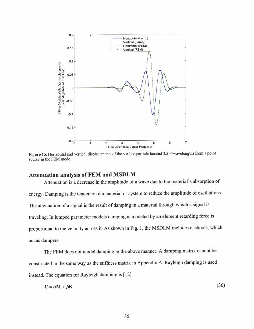
Figure 15. Horizontal and vertical displacements of the surface particle located 3.5 P-wavelengths from a point source in the FEM mode. .................................................................... 35
9

Figure 16. Phase speed error of a FEM of a material with Q=25 and angle of orientation 0 =45*........................................................................................................................................................ 3 6
Figure 17. Percent error in phase speed as a function of grid spaces per wavelength, where Q=25,angle of orientation 0 =45*. .......................................................................................................... 37
Figure 18. Number of FLOPS per S-Wavelength required for 1% phase speed error for S-wavesas v varies from 0.0 to 0.5 angle of incidence 0=450................................................................... 39
10

IntroductionNondestructive evaluation (NDE) techniques have been used for decades to characterize
materials and inspect products. For example, the U.S. Navy has developed a variety of NDE
techniques and systems for identifying defects in ship structures. These techniques and systems
are vital for finding defects before they impact the safety and mission readiness of a ship [1].
Most NDE systems contain an energy source used to probe an object, a receiver or detector that
measures how the energy has been changed by the object, and components and analyses to
record, process, and interpret the measurement data [2]. Many of these systems use ultrasonic
wave energy. Some advantages of ultrasonic testing (UT) are that small surface and subsurface
discontinuities can be detected. Ideally, the approximate size and orientation of the flaw can also
be determined [3]. Prediction and simulation of ultrasonic wave propagation provide valuable
analytical techniques in the interpretation of UT data.
Two approaches to numerical simulation of wave propagation are with a finite element
model (FEM) and a mass-spring-dashpot lattice model (MSDLM). Finite element procedures are
now a critical part of engineering analysis and design [4]. The versatility and ease of use of
commercially available finite element programs have contributed to their popularity. In recent
years, new research in mass-spring lattice models has taken place. Yim [5] discusses the
advantages of a mass-spring lattice model and the U.S. Navy has already begun research in
numerical simulation of thick, layered composites with mass-spring-dashpot lattice models [6].
In this thesis, FEM and MSDLM are compared with regard to phase speed accuracy and
computational cost.
11

Problem StatementChoosing an appropriate analysis method can be difficult without knowing which model
will most accurately represent a particular material or phenomenon.
Numerical anisotropy exists in each model and may affect computational results,
especially with regard to propagation direction [7]. It is well known that one method of reducing
error is by reducing mesh size. This does have the added effect of increasing computational cost.
This thesis proposes that by choosing carefully the model used, error and computational cost
may be reduced.
Introduction to Numerical ModelsThe mass-spring-dashpot lattice model (MSDLM) in Fig. 1 [8] is a modified version of
the mass-spring lattice model (MSLM) of Yim and Sohn [9] and Yim and Choi [10]. The
MSDLM is a heuristic, physical model where the inertia and viscoelasticity of a solid are
modeled as particles interconnected with springs and dashpots.
The spring constants and dashpot coefficients are derived from the exact partial
differential equations governing a two-dimensional standard linear solid [8]. The particle
velocities and displacements, as well as volumetric forces through each element are numerically
integrated with a fourth-order Runge-Kutta algorithm [11]. The MSDLM has been used to study
wave propagation phenomena in materials having attenuation and has been shown to agree with
analytical solutions in both steady-state and transient analyses [8].
12

2
-1-1,+j Ji1
i+Ij+1
b4h 9 93b, g.b 9
h h
(a)
Figure 1. Schematic of an MSDLM at an interior plane-strain particle located at position (ij) [8].
To ensure stability and convergence of the Runge-Kutta algorithm in the MSDLM, the Courant
number C must satisfy
c AtC = m 1.30 (1)
h
where c,nxyp is the maximum P phase speed, h is the grid space, and At is the numerical time
step [8]. Phase speed is the speed at which the crest of a single-frequency wave travels.
The finite element method is an approach for solving partial differential equations (PDEs)
and integral equations [12]. Finite element modeling of a solution involves the mesh
discretization of a continuous domain into a set of discrete sub-domains and a finite number of
points called nodes. In Fig. 2, elements comprising the entire domain are connected at common
nodes and collectively approximate the shape of the initial domain. The elements
13

are then approximated by a discrete set of piecewise continuous functions (polynomials) defined
using the nodal values of the continuous solution. The solution to the piecewise continuous
functions approximates the solution to the initial PDE. Finite difference methods are different
from finite element methods in that the differential operators are approximated rather than
represented by piecewise polynomials.
h
h
i-1,j-1il
L_
A
A
y, V
x ui-lij
i-ij-1I
MW
kij+J
A
i,iA=1
W
A
-L~
h
i+1,j+
i+1,]
i+1,j-1
w
h
Figure 2. Schematic of a four-node FEM at an interior plane-strain node located at position (ij).
In structural mechanics, finite element methods are often based on an energy principle
such as the principle of virtual work. Polynomial shape functions are used to relate the
displacement at any particular point to the displacements at the FEM nodes. A model of a
material such as a standard linear solid can be generated using the displacements at the nodes,
14
i F I RR P I
-I- V
ij-1

material properties, and constitutive relationships. FEM have been used to study wave
propagation and attenuation and have been shown to agree with analytical solutions.
To ensure accuracy and stability in a wave propagation finite element model, certain
criteria must be met. The length, Le,of a finite element must be
Le = Cmax At (2)
where c is the maximum wave speed and At is the corresponding timestep. For this analysis, an
explicit integration method is used which means the Courant-Friedrichs-Lewy (CFL) condition
must be met in order to obtain accurate results. Simply stated, the maximum allowable Courant
number C that an explicit time-integrator may use is 1.
c AtC = max (3)
Le
where Le corresponds to the length of the finite element h. While it is well known that C greater
than 1 causes a model to become unstable, a finite element model also becomes inaccurate as C
decreases to values less than 1 [12].
Fig.3 is a mass-spring-lattice model (MSLM). It is similar to the MSDLM in arrangement
of nodes but differs from the MSDLM in that it lacks dashpots. It is useful in modeling wave
propagation phenomena in elastic materials and has been shown to agree with analytical
solutions in both steady-state and transient analyses [5,9,10].
15

77 77i -1, j+1 i+I, j+1
92h
91_2_ , i i+1,
91
h
r__ i-1,j-1 ij-1 i 1j -
h h
Figure 3. Schematic of MSLM at an interior plane-strain particle located at position (i,j) [8].
Investigation into Accuracy of an Interior PointIn this example, the material is elastic and does not attenuate, so the mass-spring-lattice
model (MSLM) is used. The phase speed accuracy can be investigated using the MSLM and a
four-node FEM with an arbitrarily oriented plane wave propagating through an unbounded
elastic media.
The equations of motion in a plane strain isotropic medium having mass proportional
damping expressed in Cartesian coordinates, are
a2U 2 v a 2u p au
at2 ax 2 axay + P 2 at
a2V a2V a 2u a 2v p avP =A+2p) +(A+P)---+p (5)
at 2 ay 2 & g, aX2 T at
where u is the displacement in the x-direction, v is the displacement in the y-direction, p is the
density, r is a time constant, and A and p are Lame elastic constants.
16

The four node finite element model discretization of eqn. (4) and eqn. (5) give the
following equations written in component form at a particle position (ij) at time t.[Appendix A]
t+At 1 + =-'-^ p I +2ui, p 1 2(ii 2 + 2) 1t p 2At ) 'I (At)2UIj(PA + I (P(At zAt)
!A+p+ 3 h2 ( ui +t ui- -2tui~) (ui +tui~- -2u (6
+ h2 ( u + ~~ u.+~ u + u - 4'u)6+ h2 h (6) t
vip 1+ p2
4 2 + vi],~ ViI'+ (+.1 ****-11 1 , -1'j-1)
j ((At) 2 r 2At (At) 2 z- 2At (At) 2
.3 2 + t +t t 2 ( IVi+ 1j 4t v)h h
A + ( 7+ 6 h2 ' i + v + v +'v,, -4'vt, (7)
where At is the numerical time step and h is the grid spacing. (A similar analysis for the MSLM
can be found in reference [8].) For stability, the Courant number C must satisfy
C = , < 1 (8)h
where cp is the longitudinal wave speed given by
C,= +2p (9)p
The shear wave speed cs is given by
CS = - (10)p
17

Analysis of accuracyTaking the two dimensional discrete Fourier transform of eqn (3) and (4) and forming the
amplification equation yields [8]
l+AI u =G'u (11)
where
I= [U u t v '~A'U '-'V] (12)
t = I'/+U '+AtV tU 'V] (13)
a b c 0
G d e 0 f (4G=L1 0 0 (14)
-0 1 0 0_
and where
2(2 3)(cos(kh)-1))-(Kh 2cos(kIh)-1)
+( 4(A +3p) j(cos(ky(hXcos(kh))-1) +L =h2(t (15)
p p(At) 2 2rAt
-2 L (sin(k h)sin(k~h))b = (16)
(At)2 2z-At
p p
(At) 2 2zAt(At2 2zAtlJ(7
18

+ + (sin(kh)sin(k,h))h
p +2P(At) 2 2rAt
Cc2(2A +3p)3h 2 I(cos(kh)-1) - j(cos(kxh) -1)
+ 4(A + 3p) (Cos(kh(cos(kh))-1)6h ))
(At)2 2vAtf = P
(At) 2 2rAt
In eqns. (12) through (17)
kX = k cos 0
k, = ksinO
The four eigenvectors of the amplification matrix G are 4 p, 4+s, -p, and c-s, where the subscripts
+ or - refer to the positive and negative phases.
The positive phase change in one time step is found from the exact dispersion relation as
e1act At = kcAt (23)
(24)eactAt = kcsA
and the positive phase change from the numerical approximation is [13]
0 numericalAt = Im{ln( ,,)}
(onumericalAt = Im{ln( ,s)}
(25)
(26)
where 4j, and 4s are the eigenvectors that correspond to the pressure or P- and shear or S-waves.
19
(18)
C 2p)(At) 2 )
p
(At) 2 2rAt
(19)
(20)
(21)
(22)

The numerical phase change can be written in non-dimensional form as
O)numericalAt = fcn{C, v, kh, 0, cor} (27)
where v is the Poisson's ratio, or is a non-dimensional frequency, k is the wavenumber, and h is
the grid spacing. (A similar analysis for the MSLM can be found in reference [8].)
Percent phase error in the numerical phase change relative to the exact phase change is defined
OnumericalAt - exactAt x 100% (28)exact
Multiplying eqn. (25) by
I/k (29)
1/k
yields
= cnumerical Cexact X 100% (30)Cexact
which is simply the percent error in wave speed.
Consider the exact and numerical dispersion relation for an elastic material with v=0.30
and a plane wave propagating along the x-axis (0=0) as shown in Fig. 4. For this example and for
the remainder of this paper, C=1 will be used. As seen in the figure, the phase error of P-waves
of both FEM and MSLM rapidly decrease despite the small number of grid spaces per
wavelength. This phenomena is due to the fact that the FEM and the MSLM solutions are equal
to the exact solution for this Poisson's ratio v=0.30 and angle of orientation 6=00. The S-wave
propagation of the FEM and MSLM differ as the normalized wavelength increases. It is
interesting to note that the S-wave phase speed error is the same for both models at Poisson's
ratio v =0.3 and angle of orientation 0=0.
Fig. 5 shows the case where Poisson's ratio v =0.3 and angle of orientation 0 =45'.
20

The only difference between Fig. 4 and Fig. 5 is the angle of orientation. The FEM P-wave error
is now significantly different due to the change in 0. The P-wave solution changed from the
exact solution to a solution that has an error inversely proportional to the number of grid spaces.
In the FEM, the P- and S- wave phase speed errors are nearly equal but the errors in the P- and S-
waves for the MSLM are different by a factor of two. The unusual behavior of the MSLM S-
wave is disregarded due to the small number of grid spaces per wavelength. At two grid spaces
per wavelength, both models are extremely inaccurate.
While it is well known that the phase errors in most numerical models vary as 6 varies, it
is interesting to note that the phase error in each model varies as v varies as well. In Fig. 6, 0=
450 and v = 0.2. The phase error of the MSLM is clearly less than the phase error of the FEM.
The difference in error between the FEM and the MSLM equates to roughly one less grid
spacing per wavelength.
In Fig. 7, 0= 450 and v =0.4. The phase speed error for the P-wave speed in the FEM is
slightly larger than the phase speed error in the MSLM. However, the S-wave speed error is
nearly one order of magnitude smaller in the FEM than in the MSLM.
21

10 1oNumber of Grid Spaces Per Wavelength
(a)
10 I0~Number of Grid Spaces Per Wavelength
(b)
Figure 4. Percent error in phase speed as a function of grid spaces per wavelength, where Poisson's ratio v =0.3 and
angle of orientation 9=00 for (a) FEM and (b) MSLM.
22
FEM P-"ave------- FEM S-wave
Io"
10
102
10
104LZJ
0.
10
10-
10- 10
-MSLM P-%,,aVe-MSLM S-wave
.2I
10"
10 7
10
10

10
10 --- MSLM4 S-waveFEM P-wave
- FEM S-wavc
. Ig
LU 104
.
1o' 10 10Number of Grid Spaces Per Wavelength
Figure 5. Percent error in phase speed as a function of grid spaces per wavelength, where the Poisson's ratio v =0.3
and angle of orientation 0 =45'.
10
- MSLM P-wave
10 MSLM S-waveFEM P-wave
- FEM S-"avc
u10 -
0
10
0)0 10 10Number of Grid Spaces Per Wavelength
Figure 6. Percent error in phase speed as a function of grid spaces per wavelength, where Poisson's ratio v =0.2 and
angle of orientation 0 =45*.
23
MSLM P-wave

'(V.
- MSLM P-wave0 -------- MSLM S-wave
- FEM P-wave-.. FFM S-wavc
10
0
10 7
U~ 10001101
Number of Grid Spaces Per Wavelength
Figure 7. Percent error in phase speed as a function of grid spaces per wavelength, where Poisson's ratio v =0.4 and
angle of orientation 0 =45'.
Typically, in engineering applications an acceptable error is known and grid spaces per
wavelength N are determined and given by
N, = 21r (31)kph
Ns = 21r (32)ksh
where Np and Ns are the number of grid spaces per P and S wavelengths respectively, kp and ks
are the respective wavenumbers, and h is the grid space.
Figure 9 is the number of grid spaces required by the MSLM to achieve 1% error or less
in phase speed as functions of Poisson's ratio and angle of incidence. Fig. 10 is the same plot for
the FEM. Note that for both the FEM and MSLM, Np and Ns are symmetric about 9= 450, which
follows from the symmetry of the models for interior particles as shown in Fig. 2 and Fig. 3. In
24

both models, the phase error of P-waves decays to zero as 0 --+0 . Holding 0=00 or 90', Ns is a
monotonically increasing function for both FEM and MSLM
There are differences in the models. In the MSLM, Np decreases as v increases while
holding 6= 45*. In the FEM, holding 0=45' and increasing v increases Np slightly. Holding
0-450 , Ns for MSLM has a minimum at v =0.3 before increasing dramatically. The FEM has a
minimum Ns at v = 0.43 before increasing. The errors in S-wave speed for the case when 0=45'
and v varies from 0.0 to 0.5 is shown in Fig. 8.
25

Page intentionally left blank
26

>20
20
18
16
14
12
10
8
6
4
2
0
0 0.1 0.2 0.3 0.4 0.5Poisson's Ratio. r
(a)
CLZU2U
*0
.2
U
00
0 0.1 0.2 0.3Poisson's Ratio. i
(b)
Figure 8. Number of grid spaces per wavelength required to achieve 1% or less phase speed error in MSLM as a functionangle of incidence 0 with respect to the horizontal axis for (a) P waves and (b) S waves.
of Poisson's ratio v, and a plane wave
U2U
*0
.2
U
Q0U
t\.)-4
C
U
a.
ZZ
a
U.*0
>20
20
18
16
14
12
10
8
6
4
2
00.4 0.5
t

Page intentionally left blank
28

9090
75
$60
45
C
30
<15
00 0.1 0.2 0.3
Poisson's Ratio. r'(a)
>2020
181614
12
10864
2
0
00)
I-0)
U,0)C)
ed2
C0I-.0)
z
, 75
0
$600
45
o 30
0.4 0.50
0 0.1 0.2 0.3Poisson's Ratio. r
(b)
Figure 9. Number of grid spaces per wavelength required to achieve 1% error or less phase speed error in FEM as a functionangle of incidence 0 with respect to horizontal axis for (a) P waves and (b) S waves.
of Poisson's ratio v and plane wave
W
CL
0
$-
Z
U,
>2020
18
16
14
12
10
86
4
20
0.4 0.5

30
25-
20-
-)15
15-
S10
z
5 --
000 0.1 0.2 0.3 0.4 0.5
Poisson's Ratio. -
Figure 10. Number of grid spaces required for 1% phase speed error for S-waves as v varies from 0.0 to 0.5 angle of
incidence 0=45*.
Investigation into Accuracy of a Point at a Traction Free Surface
Wave propagation problems involving a surface excitation and a surface response in an
elastic half-space have become known as Lamb's problems due to the efforts of Horace Lamb in
1904. Lamb's work is based on Rayleigh's discovery of surface waves in 1887. Lamb discovered
Rayleigh waves are a direct function of the source kinematics and that P- and S-waves are a
function of the time derivative of the source function [14]. An analytical solution exists for these
types of problems. (Refer to [8] or [15] for a detailed discussion of the analytical solution.)
Previously in this paper, FEM and MSLM were compared to each other for phase
speed accuracy at an interior point. FEM and MSLM displacement accuracy will be compared to
an analytical solution for a point on a traction-free boundary.
Two dimensional schematics of the FEM and the MSLM discretization of a plane strain
30
MSLM- FEM (4 Node)

elastic solid at a traction free boundary are shown in Fig. 11 and Fig. 12. The corresponding
equations of motion in indicial notation for the FEM are
I t-At u..- ' t+At Ut-At U +t+At U , t UA t -] 2Ath
2 \t Uijl_ i,j/h2
+ h2 + -2u) (33)
2 2 \ i-l,-I - +,j- 2 2 \ i-1,j tv i+t j
p (tAt V-2t v +^v )+ tAtv + 4 2p23 ('vj- 1 vAt 2 " r 2At h 2
+ t ti+,j -h (34)
* 2 \ ii-,j--iji+,j-, i j
*2h2 2 u P(IU- tui~- 2 h2 2 P( ui, U-
where At is the numerical time step, and u, and vi, are horizontal and vertical displacements
respectively. (A detailed analysis of the corresponding equations of motion of the MSLM can be
found in reference [8].)
31

boundary face
y, V
i-, x U,j i+,j
h
i-J,]-1 i,j-1 i+],j-1
h
Figure 11. Schematic of an FEM at surface plane-strain particle located at position (i,j).
boundary face
h/2
h
Figure 12. Schematic of an MSLM at surface plane-strain particle located at position (z j) [8].
Input Signal ShapeThe surface excitations in the two-dimensional numerical simulations are point loads.
The frequency content of the time-varying point load is dictated by the Gaussian-modulated
cosinusoid depicted in Fig. 13. The numerical function is
32

u(O, t)= u, exp -(2 f~t - 3)2) cos(274t - 3ff-' (35)
0.
___f10.3
0 0.5 /1 1.0
U Iff 3.0
S0
2nf, Af 2_
(Time)/(Period at Center Frequency)
Figure 13. Gaussian-modulated cosinusoidal input.
where up is the peak displacement, f, is the standard deviation cyclic frequency, and f, is the
center cyclic frequency. The maximum effective frequency of the input signal is f, +3 f,.
Maximum effective frequency relates to the minimum propagating wavelength. This minimum
wavelength is used in accuracy calculations.
Figure 14 shows the surface displacement of a particle 3.5 P-wavelengths from the point
source in the MSLM. Figure 15 shows the surface displacement of a particle 3.5 P-wavelengths
from the point source in the FEM. Twenty grid spaces per minimum wavelength are used in each
model. This grid spacing is selected to ensure less than 1% error in phase speed for an interior
particle for both the FEM and the MSLM.
33

AccuracyBoth the FEM and MSLM reproduce Lamb's solution for surface displacements of an
elastic material due to surface excitation. As shown in Fig. 14 and Fig. 15, the difference
between the analytical solution and the numerical solution is small. In the FEM and MSLM, the
phase error in both the horizontal and vertical directions is less than 2%. A detailed summary of
Lamb's solution appears in Appendix C.
0.2
0.15f
04)
00
0
* -0.05
-0.1
-0.15
-0.2'0 1 2 3 4 5 6 7
(Time)/(Period at Center Frequency)
Figure 14. Horizontal and vertical displacements of the surface particle located 3.5 P-wavelengths from a point
source in the MSLM.
34
- I
Horizontal (Lamb)Vertical (Lamb)
- Horizontal (MSLM)- Vertical (MSLM)
~
n 4
Horizontal (Lamb) IVertical (Lamb)
- Horizontal (FEM)0.15 FVertical (FEM)
0.1
0.05 -
0
94.-0.5
-0.15
-0.15
-VZ0 1 2 35 6 7(Time)/(Period at Center Frequency)
Figure 15. Horizontal and vertical displacements of the surface particle located 3.5 P-wavelengths from a point
source in the FEM mode.
Attenuation analysis of FEM and MSDLMAttenuation is a decrease in the amplitude of a wave due to the material's absorption of
energy. Damping is the tendency of a material or system to reduce the amplitude of oscillations.
The attenuation of a signal is the result of damping in a material through which a signal is
traveling. In lumped parameter models damping is modeled by an element retarding force is
proportional to the velocity across it. As shown in Fig. 1, the MSDLM includes dashpots, which
act as dampers.
The FEM does not model damping in the above manner. A damping matrix cannot be
constructed in the same way as the stiffness matrix in Appendix A. Rayleigh damping is used
instead. The equation for Rayleigh damping is [12]
C = aM +)6K (36)
35

Where C is the damping matrix, M is the mass matrix, K is the stiffness matrix, and a and / are
constants determined from two given damping ratios that correspond to two unequal frequencies
of vibration. Thus damping in the FEM is not proportional to velocity but is proportional to
mass.
In this thesis, one characteristic of damping is penetration depth (Q) (Appendix D). This
is the depth an input signal travels into a material before the amplitude of the signal is reduced to
e~" (about 4%) of its original amplitude. Initial results indicate that a damped FEM does agree
with numerical solutions determined by the MSDLM. In Fig. 16, the phase speed error of a
material with Q- 25 is shown.
7 -EXACT P-wave
-----.-- FEM P-waveEXACT S-wave
6- -----. FEM S-wavc
5-
0 0.1 0.2 0.3 0.4 0,5 0.6 0.7 0.8 0.9 1
kh/2ir
Figure 16. Phase speed error of a FEM of a material with Q=25 and angle of orientation 0=45'.
In Fig. 17, the same material is modeled with varying grid spaces per wavelength. This
shows good agreement with an analysis of the MSDLM in reference [8].
36
-- ---------- - - - -----

10
FEM P-wave--.- FEM S-wave
10[
10
7.
SW-
10'
10 ~
10
10 10 10 10'Number of Grid Spaces Per Wavelength
Figure 17. Percent error in phase speed as a function of grid spaces per wavelength, where Q=25, angle oforientation 0=45'.
Computational cost of FEM and MSDLM modelsAccuracy is not the only issue of importance for numerical simulation. Computational
cost is another issue considered in this study. Theoretically, given enough time and computing
power, extremely accurate numerical models can be generated using any numerical simulation
method. In most engineering analyses, there are limits on time or computing power available for
a specific model. A trade-off study can be completed in order to maximize accuracy while
minimizing cost. In most cases, there comes a point where additional improvement in accuracy is
not beneficial enough to justify the additional computational effort. This point varies depending
on the type of engineering problem being analyzed.
37

One method of measuring computational cost is by estimating the number of floating
point operations (FLOPS) per time step or iteration. For the FEM, the MSLM and the MSDLM,
this involves determining the number of nodes and multiplying that number by the numerical
operations (multiplies, adds, divides and subtracts) per node.
Since the FEM and MSLM use the Central Difference Method, the number of FLOPS
can be easily determined. For the FEM, the number of numerical operations can be found by
examining eqn. (6) and eqn. (7). The number of nodes can be determined by using the desired
accuracy to find the number of elements needed to reach this accuracy. There are 38 numerical
operations per time step per node for the FEM.
The discretized equations of motion for the MSLM are
t+At u,, - 2 'ui,, + '-^'Ui,= (+ p+tu
P- (A&t)2 h h2 u,,,,Q -2 ui,,j u-
+ 2 (u,+1, ,+'ui 1 ,_,_ +u,,j1 +'ui1 ,1 +1 -4'u,1 ) (37)
+ 4h2 ('v,,,+ 'v,_ _ 'i+Iv
t+tvi, -2' vi, +'t-^' vi, (t + ij, p2v~ ,'P+ (At) 2 = h2 vv1 -2 +
+ ('v, +'vi, _ + ,+ ' v +'v,_ l -4'vi,) (38)
+ 4h2 ui+,j+ '+ ,_,1- u ,- u
There are 34 numerical operations per time step per node for the MSLM. Figure 18 is a
plot of the number of FLOPS per S-Wavelength required for 1% phase speed error for S-waves
as v varies from 0.0 to 0.5 angle of incidence 6 =45*.
38

60 - ------- -- 1--.-.---.-,----------- --- r-- MSLM- FEM (4 Node)
550
500
450
400
350
300'0 0.1 0.2 0.3 0.4 0.5
Poisson's Ratio. r
Figure 18. Number of FLOPS per S-Wavelength required for 1% phase speed error for S-waves as v varies from 0.0
to 0.5 angle of incidence 0 =45'.
Determining the FLOPS for the MSDLM is more difficult, since the integration method
used is a fourth order Runge-Kutta. Once the number of numerical operations is determined by
examining eqn. (36) and eqn. (37), that number must be multiplied by four. Some computational
savings are found since the MSDLM requires a Courant number of 1.3. This larger Courant
number leads to a larger time step, therefore, there are fewer nodes in the model. The stress-
dynamic equations for the MSDLM are
39
. . .. . .. ..... .........

2 \-ui+,j - i,j + (i-Mjdt T & 2
+ r(ui+,j+ i-,j- + i+,j-+1 i--,j+l i,j/
+r( - M)-+ 2 (i+ 1,j+1 + i-,j-1 i+,j-1 i-1,j+
4t2 (40)
+ H 2 M (i+ - 2i +i-
M ( + + + + _,+ -4)
+ -M. . .+ 4h2 i+l,j+l + i-1,-~,j-1 j -1 E-,j+l,
+_ - (41)*
2 \ -i,j+ -i,j 4,j- dt p rh
2rM2
" \ - i+lj+ i-I,j-1 bi+z,j- fi-),j(I4442 +,j -,- +,- -,+ (40)
+ T h 2 M (i,j+l - 2*in - v )~
+M
'u', = d~i (41)dt
''', = *in (42)dt
-zi (f x + f x (43)dt p iJ ~
'''j~ = (fbz + fz (4dt =p i.* ij(4
There are 288 numerical operations per time step per node for the MSDLM. Stress-
dynamic equations are used for the MSDLM to account for changes in volumetric forces. These
forces must be included for the stress relaxation mechanism in the MSDLM.
40

The surface stress-dynamic equations for the MSDLM and the equations of motion for
the FEM and the MSLM are different from the interior equations. For most engineering
problems, the number of surface particles is minuscule compared to the number of interior
particles and so are neglected in this study. The computational cost of a four-node FEM is
approximately the same as that for the MSLM. The computational cost of the MSDLM is on the
order of 5 times greater than the cost of the FEM and MSLM.
ConclusionsFinite element, mass-spring lattice, and mass-spring-dashpot lattice models are powerful
numerical simulation tools. For modeling elastic materials with Poisson's ratio between 0.0 and
0.2, the mass-spring lattice model has the lowest computational cost for phase speed error less
than 1%. For modeling elastic materials with Poisson's ratio between 0.35 and 0.45, the finite
element model is more accurate but costs just slightly more than the mass-spring lattice model.
For modeling materials with attenuative properties, the MSDLM is more accurate but is nearly 5
times more expensive than the finite element model. Both the FEM and MSDLM model
attenuative materials accurately.
41

References1. Nguyen, L., J. Beach, and E. Greene. International Maritime Defence Exhibition. Singapore.
(1999).
2. Logan, C., Advancing Technologies and Applications in Nondestructive Evaluation, [Online]Available http://www.llnl.gov/str/Logan.html, (February 2, 2006).
3. Hellier, C. Handbook ofNondestructive Evaluation, p. 7.110-7.111. McGraw-HillCompanies, Inc., New York (2001).
4. Bathe, K, Finite Element Procedures, p. xiii. Prentice Hall, New Jersey, (1996).
5. Yim, H and Y. Sohn, Transactions on Ultrason. Ferroelectr. Freq. Cont. 47:549 (2000).
6. Small, P.D., Ultrasonic Wave Propagation in Thick Layered Composites ContainingDegraded Interfaces, SM-NavE Thesis Massachusetts Institute of Technology, p. 12 (2005).
7. Yue, B and M. Guddati, J. Acoust. Soc. Am. 2132 (2005).
8. Thomas, A., H. Yim and J.H. Williams, Jr. submitted for publication (2005).
9. Yim, H. and Y. Sohn. IEEE Trans. Ultrason. Ferroelectr. Freq. Cont. 47:551 (2000).
10. Yim, H. and Y. Choi. Mater. Eval. 58:889 (2000).
11. Abraowitz and I.A. Stegun (Eds.), Handbook of Mathematical Functions with Formulas,Graphs and Mathematical Tables, p896-897. Dover, New York (1982).
12. Bathe, K. Finite Element Procedures. p815 Prentice Hall, Inc. (1996).
13. H. Yim. Unpublished research (2003).
14. Glaser, S. G. Weiss, L. Johnson J. Acoust. Soc. Am., 104 (3) (1998).
15. H. Lamb. Philosophical Transactions of the Royal Society Of London. Series A, ContainingPapers of a Mathematical or Physical Character. 203:1(1904).
42

APPENDIX A - Derivation of the indicial notation for the 4-node finiteelement model
The finite element method (FEM) is a widely used tool in engineering analysis [A. 1]. The
four-node element is one of the simplest, but it is still a powerful and useful tool in the solution
of practical engineering problems. In this appendix, a plane strain isotropic medium having
mass- proportional damping is discretized.
The equations of motion in the interior of a plane strain isotropic medium having mass-
proportional damping is expressed in Cartesian coordinates as
2U a2u a2v a 2u p auP 2 =(A +2p) 2 + (A + p) + (A.1)
ax axy y ata2 aX2 2~ + 2
a2 V a2V a2U ___ (A.2p_ = (A +2p) + (A~ + p (A.2)Pa~V~~ Y axay ax 2 atat 2 a22
where p is density, u and v are horizontal and vertical displacements, respectively, A and p are
Lame elastic constants and r is a characteristic time.
The corresponding elemental equilibrium equation for a lumped mass element can be
expressed in matrix form as
M +AI (el) -2' U(el)+tAtU(eI) + I (el) t+A+ - (el) tA(el)+ K(el)u el) F (el) (A.3)(At) 2 r 2At
where Mel) is the elemental mass matrix.
I
1
M (el) = ph 2 1 (A.4)4 1
43

and 'V(e') is the elemental displacement vector
I (e) _
tU
t U2
t U3
t 4
V1
V2
V3
V4
(A.5)
A schematic of a square four-node element having grid spacing h is shown in Figure Al.
3
F-
y, VA
x ,
4
h
Figure A 1. Schematic of four-node element.
The elemental stiffness matrix K ") may be calculated as
K(el) = f f B(el)T C B(e)B(e)dxdy
h
(A.6)
44
t

H(el) is the displacement interpolation matrix for a four-node square element i with sides of
length h
He') = h10
h2 h3 h4 0 0 0 00 0 0 h h2 h 3 h4
where
I 2xh, =.-Ci+-7J1ih 4 h
12xh2 = - h 1
4 h
(A.8)
(A.9)2y)
(A.7)
h3 = I ( _ (A.104 h h
h4 = - (+ 1 (A.114 h 2h
B (e) is the corresponding strain-displacement matrix corresponding to the local element degrees
of freedom, given as
hB,)B (el= 0
_h,,
h2,x h3j h4j 0 0 0 0
0 0 0 h1 , h2,, h3, h4 ,
h2,, h3 , h4,y h1 , h2,x h3 h4,x
(A.12)
where
45
)
1+2 J2 h
hI ! C ( Y2(A.13)2 h
1+ 2
h2,x = h h (.4
2 h
1-2-
1h
h -1 ( (A.16)2 h1+2-
1h
h4,y I (C_+22 (A.216)2 li
hie r (2 j (A.17)2 h
1-2-1h
h2,y = 2 h A.8
-2 h
h3,y = 2) h(.19)
-2 h
h4,= 2 h (.0
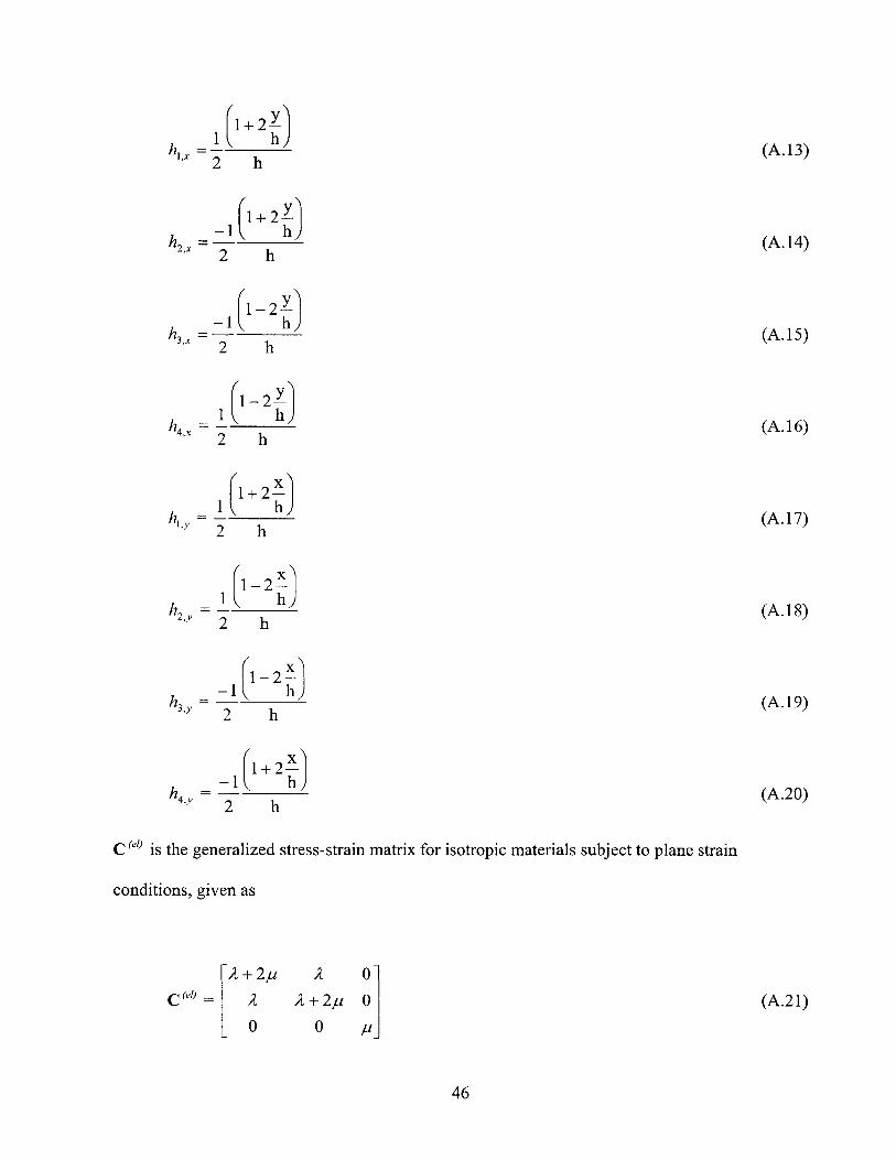
C' is the generalized stress-strain matrix for isotropic materials subject to plane strain
conditions, given as
A+2p A 0
C' =el A A +2p 0 (A.2 1)
0 0 P_
46

The elemental K matrix is
K(el) =
k3 k4 k5 k6 k7 k8
k4 k3 k8 k7 k6 k5
ki k2 k7 k8 k5 k6k k6 k5 k 8 k7
k k4 k3 k2
k k2 k3
ki k4
where
ki 1 A + p3
k2 = p3 2
k3 = - -6
k4 = -26
2
k5 = IA+ Ip4 4
k6 = AI p4 4
k7 = 4- I A p4 4
47
(A.22)
(A.23)
(A.24)
(A.25)
(A.26)
(A.27)
(A.28)
(A.29)
k8 1k - -A +-p
4 4(A.30)
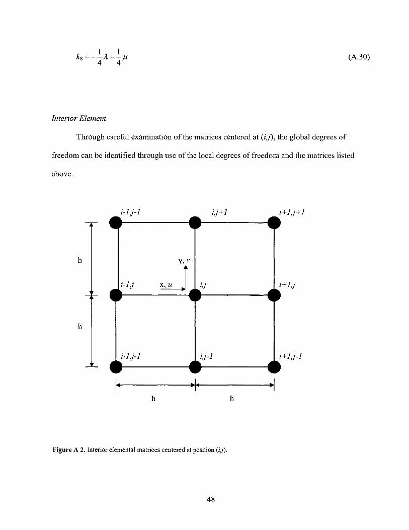
Interior Element
Through careful examination of the matrices centered at (ij), the global degrees of
freedom can be identified through use of the local degrees of freedom and the matrices listed
above.
h
h
i-1,]-1
L
A U
w
h
pp
h
Figure A 2. Interior elemental matrices centered at position (ij).
48
y, v
i-1,j-1 i~j-1ILL-i
i
+1,j-1

The four-node finite element discretization of eqns. (A. 1) and (A. 2) yields the following
equations written in component form at position (ij) and time t.
+ t+At U.) 3_2i t u +.u1 , -2tu , 1 )h
12+1T2 (,it~ + I tj, 2 i
h
+ 6 2 +(tt +1 +11 1 , -4'u ,)
+ 4 h 2 4 ( v. 1*1 l-I il~~ It. 1 vi-j 1 -ti],
P 1 ( -vt-AtU + tvAt U
z- 2At
PAt
h 2 i+ 1j i-i,]
ht+Ay ( 3h,2+1 vij - 2v )
-2tv, 1 )
I A + I+ 6 2 2P+ v +'v, +'vi1,j+_ -4'v )
+ h4 2 4 ui ~ ~ - ui~~- + ui_,_ _u )1j
P 1 (1-Atv. + t+A v-r 2At
where At is the numerical time step.
49
(A.31)
(A.32)
I -t U
(t-At vi, -2 v.,

Surface Element
Through examination of the matrices centered at (ij), the global degrees of freedom can
be identified through use of the local degrees of freedom. A two-dimensional schematic of the
FEM discretization of a plane strain elastic solid along a traction boundary is shown in Figure A
3.
h
A
F
y, v
xui-1j
h
boundary face
i~i
F!
Figure A 3. Schematic of a surface element centered at (i,j).
The corresponding equations of motion are
50
i-1,j- ij-1
i+1,j
+1,j-]
W

2t-At t+At )t-At u + t+At +, 3,+I ( + t tA r 2At h
2
( Uijt _1 U i~ lj-h
+h2 Q - v+tUi+j- -2u-)
+ 2 h2 2 r( tjvi' -I'v- 1 21 h 2 2t ViI' )tVi
1t-2,j r 2At j
2 \ i-,jvi+,j -2'v,j)
h+ 2 (t~i, -+tvi+11j-1 -2'v )
I2 I+ 2 211t 1-u h 2 2 (tu tu)
Where At is the numerical time step, and uj, and vi, are the horizontal and vertical displacements,
respectively.
REFERENCES
[A-1] Bathe, K, Finite Element Procedures, Prentice Hall, New Jersey, 1996.
51
(A.33)
(A.34)
+t+At Vj 3h2p i' - tvij)

Page intentionally left blank
52

APPENDIX B - Dispersion Relation/ High frequency assumptionIn order to make numerical analysis of elastic wave phenomena possible, assumptions
concerning the dispersion relation and frequency of the wave must be made. In this appendix, the
dispersion relation for a material having mass-proportional damping is derived.
Equilibrium equation
The equation of motion for a one-dimensional material having mass-proportional
damping is
EaU 2 a a
ax + at C2 (B.1)
where E is the governing elastic constant, u is the displacement, p is the density, and r is a
characteristic time.
Consider a propagating harmonic wave having the form
u(x,t) = U~e-"+i(->t) (B.2)
where U is the peak displacement, a is the attenuation, k is the wavenumber, and o is the radial
frequency.
Solving for the partial derivatives yields
a2 2 = U 0 (a 2 -k 2 + > - U0 (2aik)e -+ika (B.3)
11lt = UOicte-cf+'(kx-"> (B.4)
a2u at2 = -UCO22e-c+ika) (B.5)
After substituting eqns. (B.3) through (B.5) into eqn. (B.1) and simplifying, the
dispersion relation becomes
53

E(a2 -k 2 )pco 2 = E(2aik) - ico
Separating the real and imaginary parts of eqn. (B.6) yields
E(a2 -k 2 )+pCo 2 =0
E(2aik) - --io = 0T
Solving eqn. (B.8) for the wavenumber yields
k = P ozE2a
Substituting eqn. (B.9) into eqn. (B.7) yields
2)
E a2 _ (a L+ CO2 = 0
P
Let
S= Cmaxp
Multipyling eqn (B. 10) by a2 and substituting eqn. (B. 11) into eqn. (B. 10) yields
4 2 2a2a- 4
2A 4 + 2=0Cmax
54
(B.6)
(B.7)
(B.8)
(B.9)
(B.10)
(B.11)
(B.12)T 4cmax

Solving for a2 yields
a 2 CO -+ I+12C max l2 2- a ))
Substituting eqn (B. 13) into eqn. (B.7) yields
k2=W 2 2 +
2cmax2
At high frequencies,
k -'Cmax
1a-
2 cmax T
At low frequencies,
k
1+ j2
1
2vc max
a -+2a2
55
(B.13)
(B. 14)
(B.15)
(B.16)
(B.17)

Page intentionally left blank
56
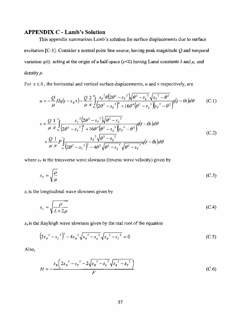
APPENDIX C - Lamb's SolutionThis appendix summarizes Lamb's solution for surface displacements due to surface
excitation [C-I]. Consider a normal point line source, having peak magnitude Q and temporal
variation q(t), acting at the origin of a half-space (y<O) having Lame constants A and u, and
density p.
For x < 0 the horizontal and vertical surface displacements, u and v respectively, are
Q Q 2* s 02-s -L2 ST _2Q Hq(tsT T 2 q(t- Ox)d (C.1)
II PZS,(20 2) 1604(02 -SL2S T _02)
Q 1 sT2 (202 -ST2 W2 -SL2 q t_9x)df (202 2Y +164(02 ~ 22 2)
S S 1 L XT -2(C.2)
+Q 1 fsT 2 -sL -q(t - OxcdOA sT22 -sT -4 L 2 s2 T
where sT is the transverse wave slowness (inverse wave velocity) given by
ST = (C.3)
SL is the longitudinal wave slowness given by
sL (C.4)S+ 2p
sR is the Rayleigh wave slowness given by the real root of the equation
(2sR2 ST 224SR2 2SL S =0 (C.5)
Also,
H =L 5 R sT (C.6)F
57

where
4 -2ss2 sR L3( S T 4sR ~ 4,R5 4sR3 R ~sL2 5R2 7ST -8ST 2SR (C
s2 ~S2 R2 T2SR SL ISR ST
P in eqn. (C.2) denotes the principal value of the integral [C-2]. A non-integrable singularity
exists at 0= sR and the integral must be defined as
b 'C-6 b
P f(#4 = Jim ff( )d + ff( )dj (C
where a<c<b and the non-integrable singularity exists atf(c).
The surface displacements for x<0 are given by replacing (t - ;x) with (t + 4x) in eqns.
(C.1) and (C.2) and reversing the sign of the horizontal displacements in eqn. (C.1).
REFERENCES
[C-1] H. Lamb. Philosophical Transactions of the Royal Society of London. Series A,Containing Papers of a Mathematical or Physical Character. 203:1 (1904).
[C-2] E. Kreyszig. Advanced Engineering Mathematics 7th ed., p.851. John Wiley& Sons, NewYork (1993).
58
.7)
.8)

APPENDIX D - Penetration DepthLet the penetration depth Q of an attenuative material be the number of wavelengths required for
a cyclic input signal to decrease in amplitude to e-" where a is the attenuation and x is the
distance.
e-aQA = e-n (D.1)
where A is the wavelength
aQA = rc (D.2)
Q = '' (D.3)F a A
For a standard linear solid [Dl] having a relaxation time r , under the frequency assumption
COr >> (D.4)
where co is the circular frequency. Frequency-independent attenuation is
1a =
2-c
where c is maximum phase speed. Recall,
c = Af
where f is cyclic frequency. The relationship between co andf is
co= 27f
therefore
(Of= -
Substituting eqn. (D-5) into eqn. (D-3) yields
ff2rc -=. Q
(D.5)
(D.6)
(D.7)
(D.8)
(D.9)
Substituting eqn. (D-6) into eqn. (D-9) yields
59

;r21f = Q (D.10)
Substituting eqn. (D-8) into (D- 10) yields
rc = Q (D.11)
Recall,
COc=- (D.12)
k
where k is the wavenumber. k can be rewritten as
k= O I+ + (D.13)-cmax
The phase speed error between the exact solution and the numerical approximation can be
written as
error = c - max (D.14)C max
Substituting eqn. (D-12) into (D-14) yields
(O
error = k m (D.15)Cmax
Substituting eqn. (D-13) into (D-15) yields
error = 1 1+ I+ 2 -I (D.16)
Figure D 1 is a plot of the error with respect to cor. The error decreases as the frequency
increases. As wor increases, Q increases. Therefore a material having a high penetration depth,
which is equivalent to a low attenuation, is modeled more accurately.
60

*'.u~nu'u-'np r n.u ............ .. .~i ..... ii-i-mI- -.- ---AM
0
10 0
10
10-
10'
10
10
10-1
10710F3
10-2 10
Figure D 1. Phase speed error as a function of cor.
Error in attenuation
Attenuation may be written as
a = O -+ 1 + IT 2r al tmeca22lJ
recall that numerically
_1amax~
2rcmax
The error between the exact and numerical attenuation can be written as
61
1000 T
10 1 102 103
(D.17)
(D.18)
- I I 1 11 1 1 I . I I
II I . , . . . , I . . I I I I . I I . . I . . . . I , . - -
.I . -

error = amax -aamax
Substituting eqn. D- 18 and C-19 into eqn. D- 17 yields
error =1I-Fir{-1+ 1+ 2
Figure D 2 is a plot of the attenuation error as a function of cor. As Cor increases, the error
decreases.
0
0)
100
10
10-2
10
10 -
10
1
10
06L
10-2 10~1 100oT
10 1 102 103
Figure D 2. Attenuation error as a function of cnr.
62
(D.19)
(D.20)
........ .. ......
10-3
If a material is attenuative, its penetration depth decreases. Since penetration depth is a
function of wcr , the frequency decreases as well. This decrease in frequency causes errors in
phase speed modeling.
REFERENCES
[D-1] Thomas, A., H. Yim and J.H. Williams, Jr. submitted for publication (2005).
63

Page intentionally left blank
64qCvT