Remote Sounding with Advanced Infrared and Microwave Instruments

Chris BarnetNOAA/NESDIS/STAR

University of Maryland, Baltimore County (Adjunct Professor)AIRS Science Team Member

NPOESS Sounder Operational Algorithm Team MemberGOES-R Algorithm Working Group – Chair of Sounder Team

NOAA/NESDIS representative to IGCO

Wednesday July 25, 2007Workshop on Applications of Remotely Sensed

Observations in Satellite Data Assimilation

2

Sounding Theory Notes for the discussion today is on-line

voice: (301)-316-5011 email: chris.barnet@noaa.govftp site: ftp://ftp.orbit.nesdis.noaa.gov/pub/smcd/spb/cbarnet/..or.. ftp ftp.orbit.nesdis.noaa.gov, cd pub/smcd/spb/cbarnetSounding NOTES, used in teaching UMBC PHYS-741: Remote Sounding and UMBC PHYS-640: Computational Physics (w/section on Apodization)

~/reference/rs_notes.pdf

~/reference/phys640_s04.pdfThese are living notes, or maybe a scrapbook – they are not textbooks.

For an excellent text book on the topic of remote sounding is:

Rodgers, C.D. 2000. Inverse methods for atmospheric sounding: Theory and practice. World Scientific Publishing 238 pgs

3

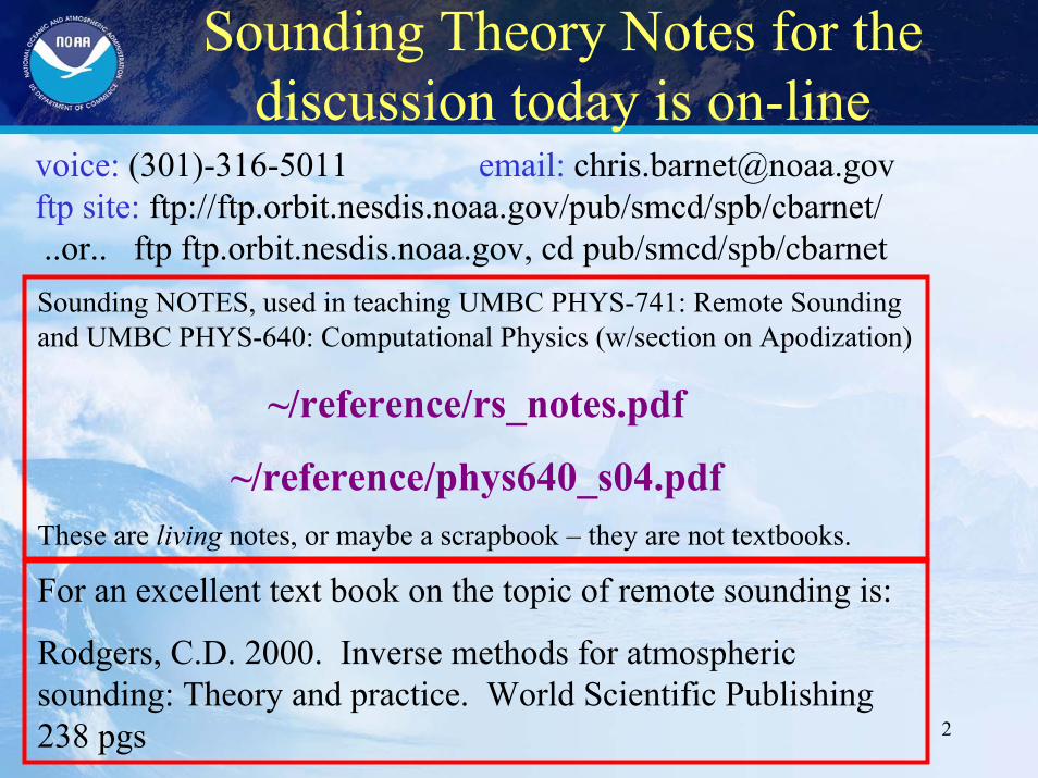
Topics for Lectures

• Monday July 23, 2007– Introduction to AIRS & IASI and our plans to use operational sounders

to retrieve atmospheric and surface products.– Introduction to Sounding Methodology

• Cloud clearing• Statistical Regression Retrievals

• Tuesday July 24, 2007– Sidebar: Comparison of Dispersive and Interferometric Instruments– Introduction to Sounding Methodology (continued)

• The forward model: Converting state vector to radiances.• The inverse problem: Converting radiances to a state vector.

• Wednesday July 25, 2007– Introduction to Sounding Methodology (continued)

• Vertical Averaging Kernels & Error Covariance Matrices– Validation of Products– Atmospheric Carbon Retrievals

4

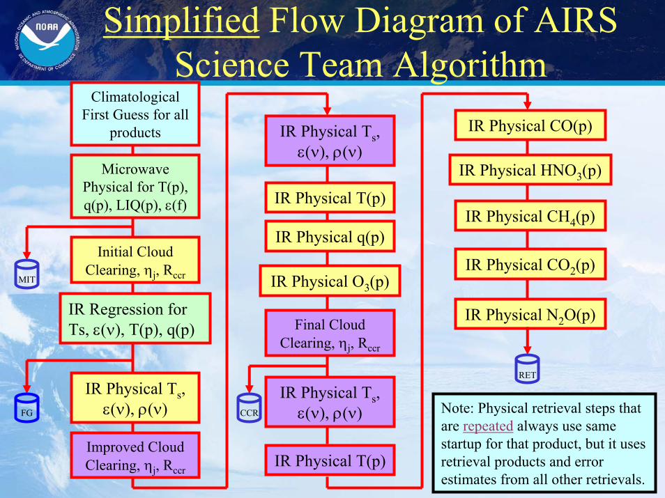
Simplified Flow Diagram of AIRS Science Team Algorithm

ClimatologicalFirst Guess for all

products

Initial Cloud Clearing, ηj, Rccr

IR Regression for Ts, ε(ν), T(p), q(p)

IR Physical Ts, ε(ν), ρ(ν)

Microwave Physical for T(p), q(p), LIQ(p), ε(f)

Improved Cloud Clearing, ηj, Rccr

Final Cloud Clearing, ηj, Rccr

IR Physical CO(p)

IR Physical HNO3(p)

IR Physical CH4(p)

IR Physical CO2(p)

IR Physical Ts, ε(ν), ρ(ν)

IR Physical T(p)

IR Physical T(p)

IR Physical Ts, ε(ν), ρ(ν)

IR Physical q(p)

IR Physical O3(p)

IR Physical N2O(p)

MIT

RET

FG Note: Physical retrieval steps that are repeated always use same startup for that product, but it uses retrieval products and error estimates from all other retrievals.

CCR

5

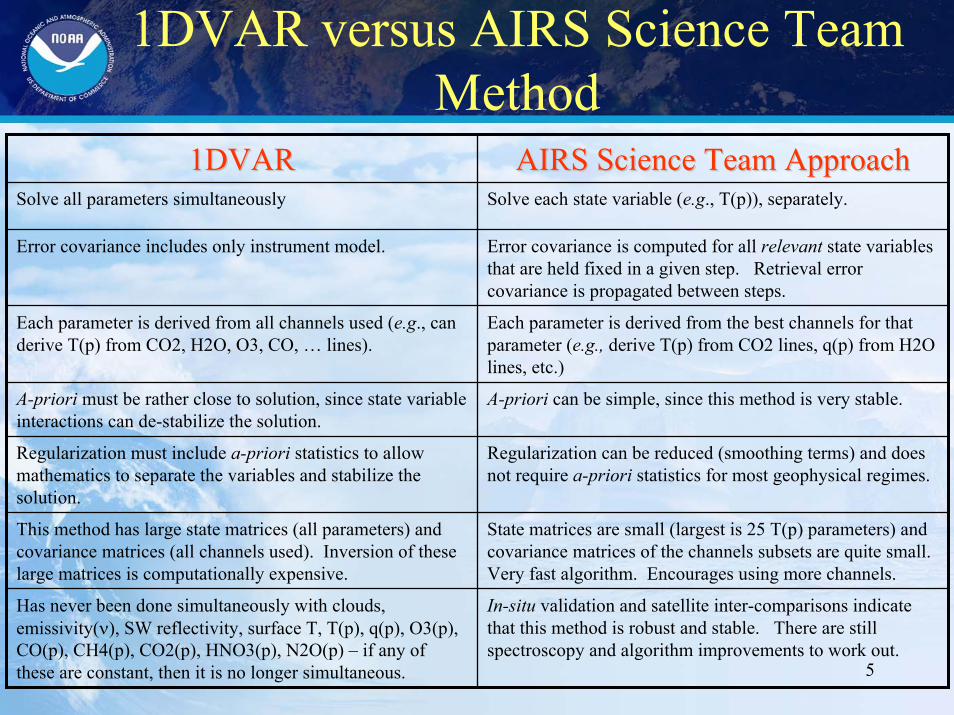
1DVAR versus AIRS Science Team Method

In-situ validation and satellite inter-comparisons indicate that this method is robust and stable. There are still spectroscopy and algorithm improvements to work out.

Has never been done simultaneously with clouds, emissivity(ν), SW reflectivity, surface T, T(p), q(p), O3(p), CO(p), CH4(p), CO2(p), HNO3(p), N2O(p) – if any of these are constant, then it is no longer simultaneous.

State matrices are small (largest is 25 T(p) parameters) and covariance matrices of the channels subsets are quite small. Very fast algorithm. Encourages using more channels.

This method has large state matrices (all parameters) and covariance matrices (all channels used). Inversion of these large matrices is computationally expensive.

Regularization can be reduced (smoothing terms) and does not require a-priori statistics for most geophysical regimes.

Regularization must include a-priori statistics to allow mathematics to separate the variables and stabilize the solution.

A-priori can be simple, since this method is very stable.A-priori must be rather close to solution, since state variable interactions can de-stabilize the solution.

Each parameter is derived from the best channels for that parameter (e.g., derive T(p) from CO2 lines, q(p) from H2O lines, etc.)

Each parameter is derived from all channels used (e.g., can derive T(p) from CO2, H2O, O3, CO, … lines).

Error covariance is computed for all relevant state variables that are held fixed in a given step. Retrieval error covariance is propagated between steps.

Error covariance includes only instrument model.

Solve each state variable (e.g., T(p)), separately.Solve all parameters simultaneously

AIRS Science Team ApproachAIRS Science Team Approach1DVAR1DVAR

6

Some Final Thoughts on Remote Sounding Approaches

• This discussion isn’t new. It has been going on for more than 30 years!

• It really boils down to Physics versus Statistics – although in the modern era this distinction has been blurred.– Regression and Neural Network Approaches– Use of geophysical covariance to regularize the under-determined problem.

• Take a look at discussion at the end of Rodgers, C.D. 1977. “Statistical principles of inversion theory.” in ”Inversion Methods in Atmospheric Remote Sounding” (ed. Deepak) p.117- 138.

• This discussion is also transcribed in Section 22.2 of my notes (reference/rs_notes.pdf).

• As in all things, the answer may lie in the middle ground. Weare exploring adding some a-priori statistics to help in certain geophysical domains (e.g., lower boundary layer T(p), etc.) and we may explore some simultaneous retrievals (T(p)/emissivity, etc.) to improve the products.

7

Retrieval Averaging Kernels (11 slides)

See

1)Rogers 2000, pg. 43-44 & pg. 83-85

2)Rodgers and Conner 2003

3) My notes – section 8.12.1

8

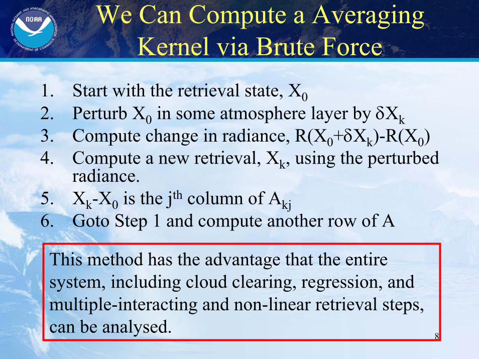
We Can Compute a Averaging Kernel via Brute Force

1. Start with the retrieval state, X02. Perturb X0 in some atmosphere layer by δXk3. Compute change in radiance, R(X0+δXk)-R(X0)4. Compute a new retrieval, Xk, using the perturbed

radiance.5. Xk-X0 is the jth column of Akj6. Goto Step 1 and compute another row of A

This method has the advantage that the entire system, including cloud clearing, regression, and multiple-interacting and non-linear retrieval steps, can be analysed.

9

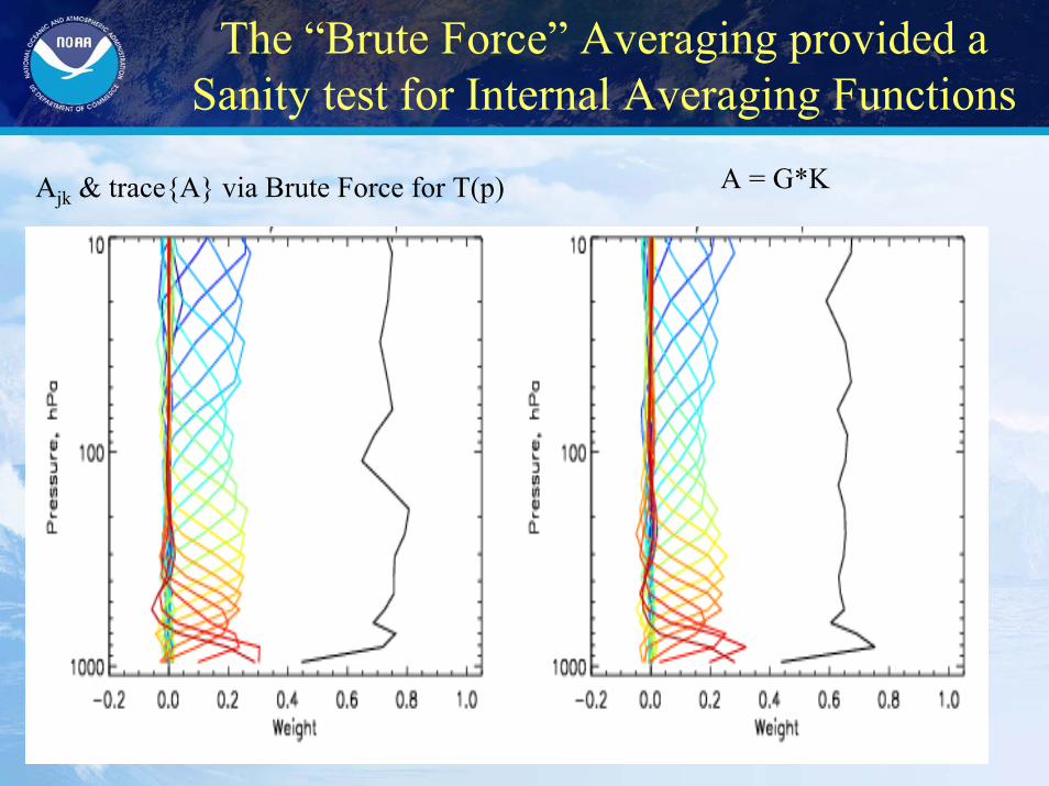
The “Brute Force” Averaging provided a Sanity test for Internal Averaging Functions

A = G*KAjk & trace{A} via Brute Force for T(p)

10

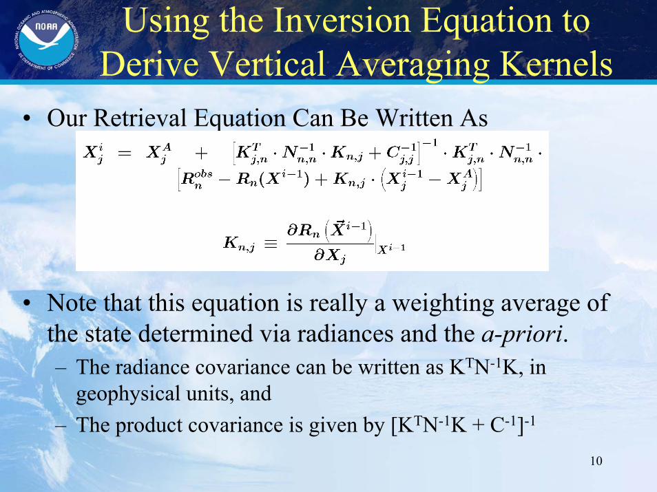
Using the Inversion Equation to Derive Vertical Averaging Kernels

• Our Retrieval Equation Can Be Written As

• Note that this equation is really a weighting average of the state determined via radiances and the a-priori.– The radiance covariance can be written as KTN-1K, in

geophysical units, and– The product covariance is given by [KTN-1K + C-1]-1

11

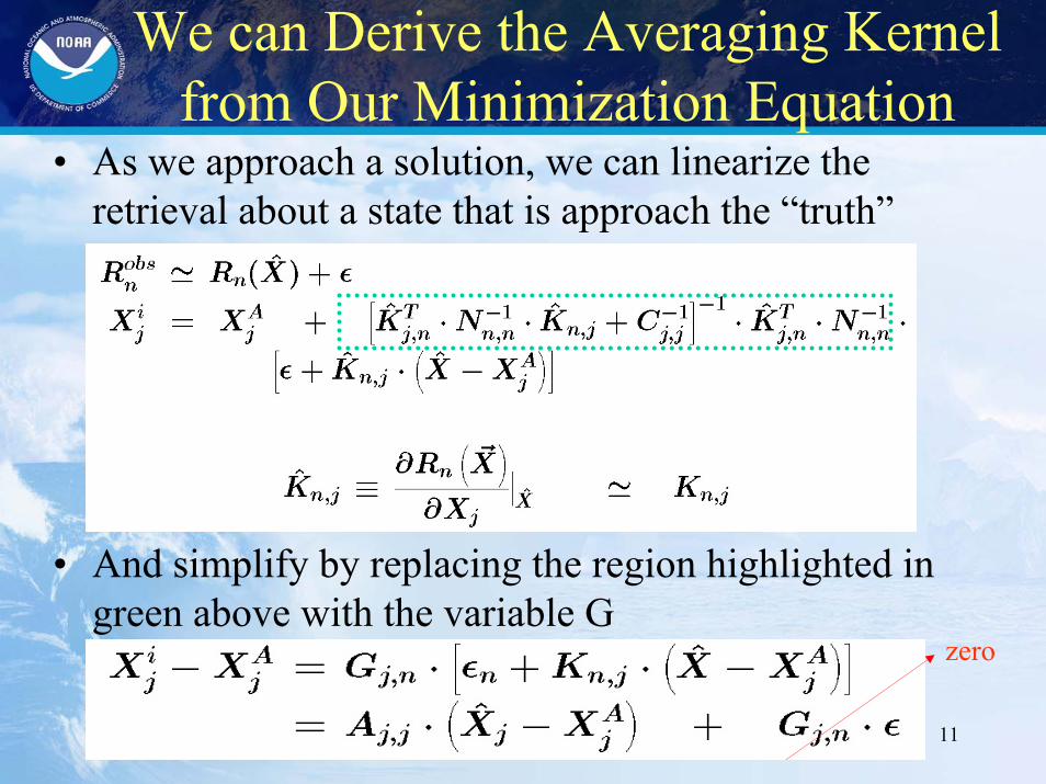
We can Derive the Averaging Kernel from Our Minimization Equation

• As we approach a solution, we can linearize the retrieval about a state that is approach the “truth”

• And simplify by replacing the region highlighted in green above with the variable G

zero

12

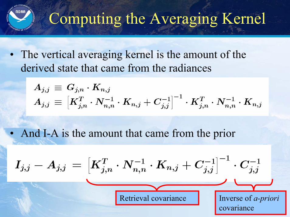
Computing the Averaging Kernel

• The vertical averaging kernel is the amount of the derived state that came from the radiances

• And I-A is the amount that came from the prior

Retrieval covariance Inverse of a-prioricovariance

13

Value of the Vertical Averaging Function

• A is the retrieval weighing of the channel kernel functions (think of a retrieval operator as an integrator of data)

• A tells you how much the observations were believed.• I-A tells you how much of the a-priori was believed.• When comparing other measurements (such as high vertical

resolution sondes or aircraft) the validation measurements – Must have similar vertical smoothing and– Should be “degraded” by the fraction of the prior that entered the solution

(i.e., in regimes were we don’t have 100% information content)• When using AIRS products the A matrix

– Tells you the vertical correlation between parameters– Tells you how much to believe the product and where to believe the

product.– A-priori assumptions can be removed from the solution if we are in a

linear domain.

14

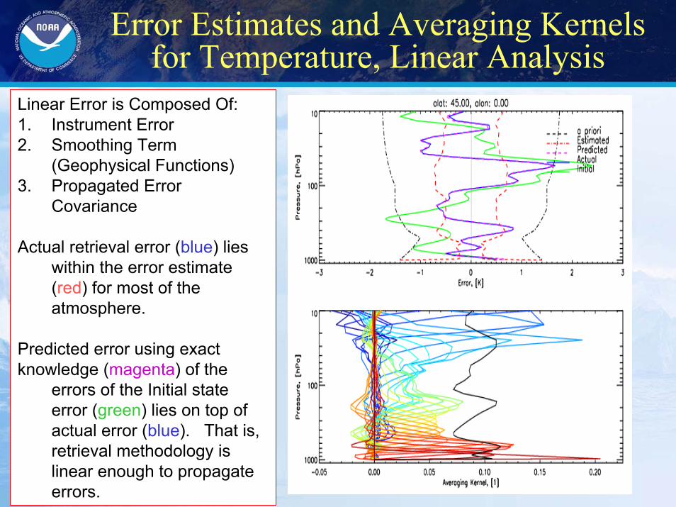
Error Estimates and Averaging Kernels for Temperature, Linear Analysis

Linear Error is Composed Of:1. Instrument Error2. Smoothing Term

(Geophysical Functions)3. Propagated Error

Covariance

Actual retrieval error (blue) lies within the error estimate (red) for most of the atmosphere.

Predicted error using exact knowledge (magenta) of the

errors of the Initial state error (green) lies on top of actual error (blue). That is, retrieval methodology is linear enough to propagate errors.

15

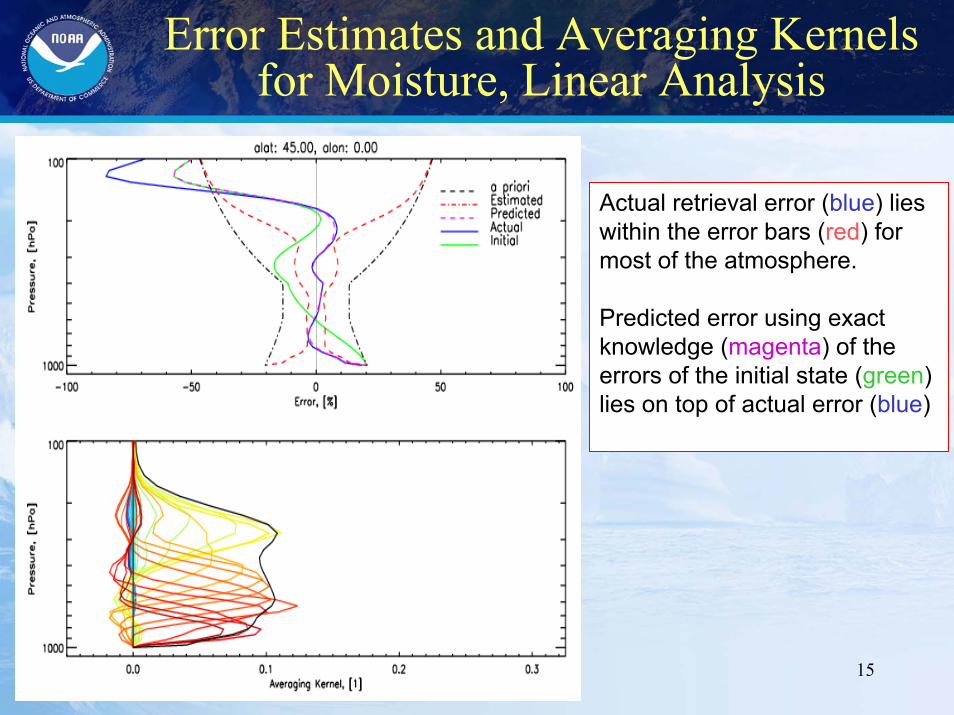
Error Estimates and Averaging Kernels for Moisture, Linear Analysis

Actual retrieval error (blue) lies within the error bars (red) for most of the atmosphere.

Predicted error using exact knowledge (magenta) of the errors of the initial state (green) lies on top of actual error (blue)

16

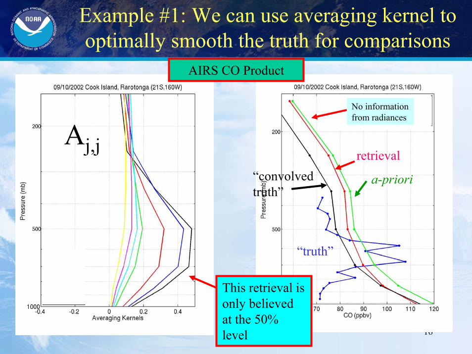
Example #1: We can use averaging kernel to optimally smooth the truth for comparisons

Aj,j

“truth”

a-priori

retrieval“convolved truth”

This retrieval is only believed at the 50% level

AIRS CO Product

No information from radiances

17

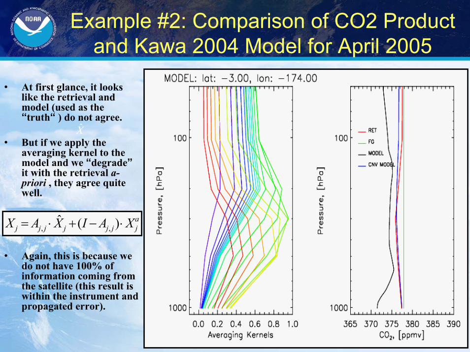
Example #2: Comparison of CO2 Product and Kawa 2004 Model for April 2005

• At first glance, it looks like the retrieval and model (used as the “truth“ ) do not agree.

• But if we apply the averaging kernel to the model and we “degrade”it with the retrieval a-priori , they agree quite well.

• Again, this is because we do not have 100% of information coming from the satellite (this result is within the instrument and propagated error).

ajjjjjjj XAIXAX ⋅−+⋅= )(ˆ

,,

X̂

18

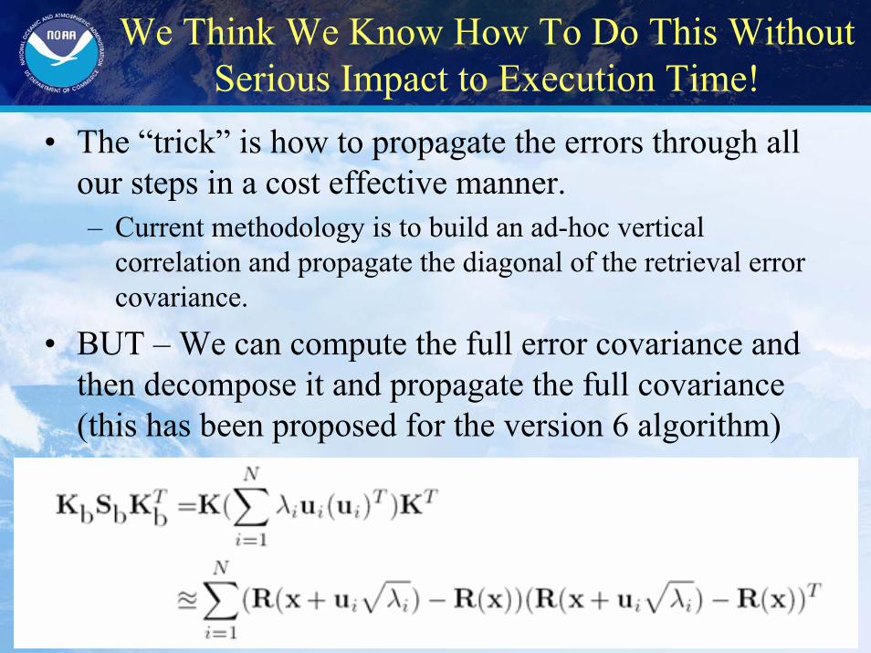
We Think We Know How To Do This Without Serious Impact to Execution Time!

• The “trick” is how to propagate the errors through all our steps in a cost effective manner.– Current methodology is to build an ad-hoc vertical

correlation and propagate the diagonal of the retrieval error covariance.

• BUT – We can compute the full error covariance and then decompose it and propagate the full covariance (this has been proposed for the version 6 algorithm)

19

Validation (17 slides)

20

“what is truth”• Compare to ECMWF & NCEP Analysis (e.g., Susskind, 2005)

– Can compare complete global dataset– Differences can be model or retrieval errors– Implicitly validating against all other instruments (all assimilated space-borne,

sondes, buoy’s etc.) used in analysis• Compare to Radiosondes, Ozonesondes (e.g., See Tobin, 2006, Divakarla, 2006)

– Only a couple hundred “dedicated” sondes are flown per year. Usually we fly 2 sondes so we can see lower and upper air at overpass time.

• Sondes can take 1-2 hours to ascend• Sondes can drift 100’s of km’s during ascent.

– A few hundred sondes are launched globally per day (usually at synoptic times) that are within 300 km and +/- 1 hour of our overpass.

• Different sonde instruments, quality of launches, etc.• In-situ intensive experiments with sondes, aircraft and LIDAR.

– Have participated in INTEX-NA6 AEROSE, START, MILAGRO, INTEX-B, AMMA, and WAVES

• Inter-comparison of satellite products.– Aqua/AIRS has been compared to Aura/TES/MLS/OMI (8 minutes apart),

CloudSat/Calipso (75 seconds apart) products.• Large number of global co-locations of “similar” products.

– Aqua/AIRS has been compared to other satellites (e.g., TOMS, SBUV, CERES)

21

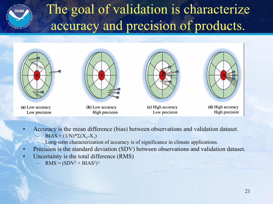
The goal of validation is characterize accuracy and precision of products.

• Accuracy is the mean difference (bias) between observations and validation dataset.– BIAS = (1/N)*Σ(X2-X1)– Long-term characterization of accuracy is of significance in climate applications.

• Precision is the standard deviation (SDV) between observations and validation dataset.• Uncertainty is the total difference (RMS)

– RMS = (SDV2 + BIAS2)½

22

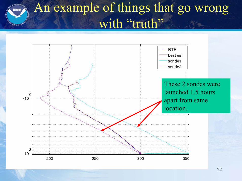
An example of things that go wrong with “truth”

These 2 sondes were launched 1.5 hours apart from same location.

23

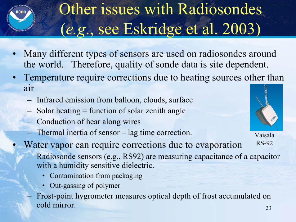
Other issues with Radiosondes(e.g., see Eskridge et al. 2003)

• Many different types of sensors are used on radiosondes around the world. Therefore, quality of sonde data is site dependent.

• Temperature require corrections due to heating sources other than air– Infrared emission from balloon, clouds, surface– Solar heating = function of solar zenith angle– Conduction of hear along wires– Thermal inertia of sensor – lag time correction.

• Water vapor can require corrections due to evaporation– Radiosonde sensors (e.g., RS92) are measuring capacitance of a capacitor

with a humidity sensitive dielectric.• Contamination from packaging• Out-gassing of polymer

– Frost-point hygrometer measures optical depth of frost accumulated on cold mirror.

VaisalaRS-92

24

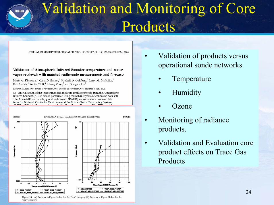
Validation and Monitoring of Core Products

• Validation of products versus operational sonde networks

• Temperature

• Humidity

• Ozone

• Monitoring of radiance products.

• Validation and Evaluation core product effects on Trace Gas Products

25

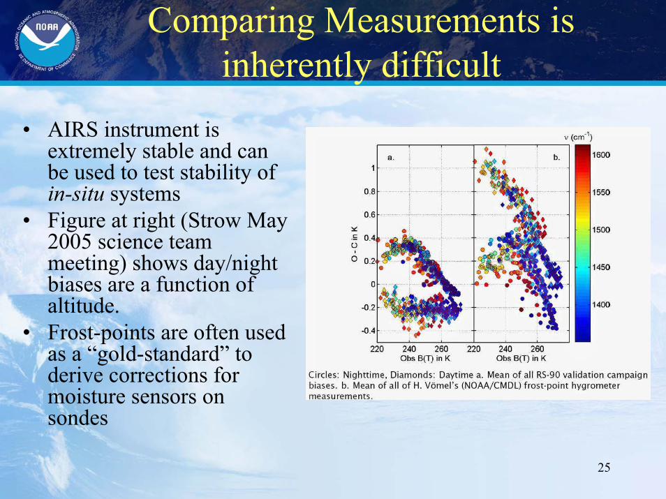
Comparing Measurements is inherently difficult

• AIRS instrument is extremely stable and can be used to test stability of in-situ systems

• Figure at right (Strow May 2005 science team meeting) shows day/night biases are a function of altitude.

• Frost-points are often used as a “gold-standard” to derive corrections for moisture sensors on sondes

26

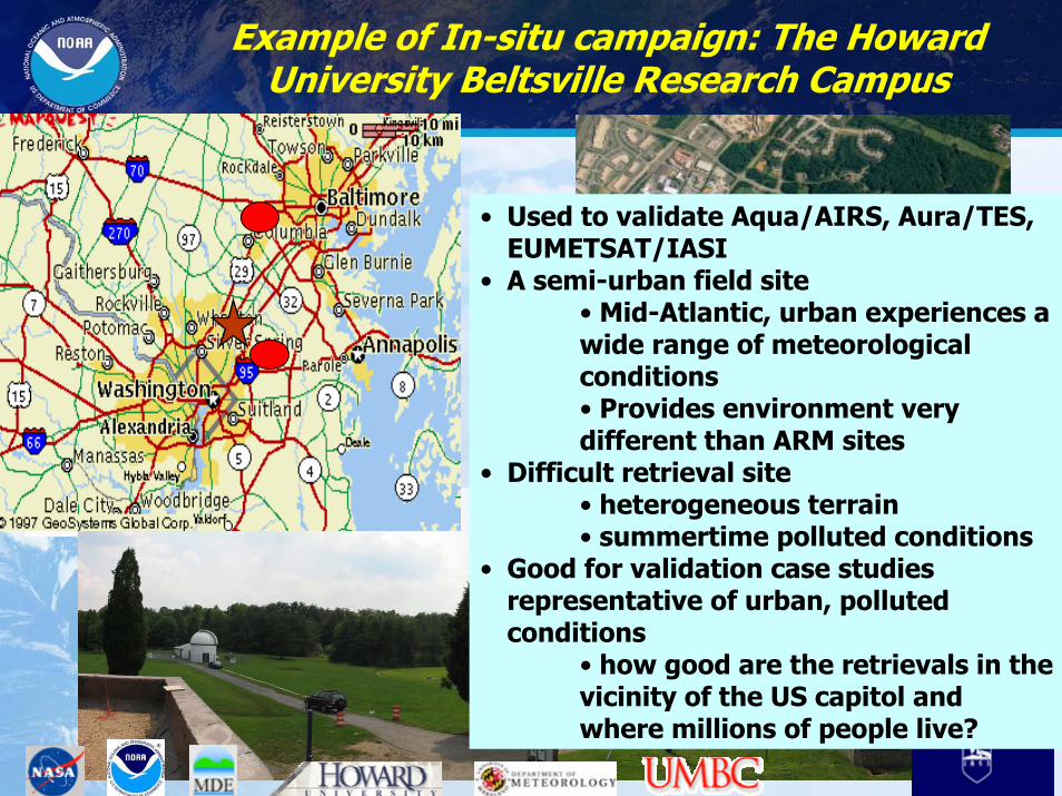
Example of In-situ campaign: The Howard University Beltsville Research Campus

• Used to validate Aqua/AIRS, Aura/TES, EUMETSAT/IASI

• A semi-urban field site• Mid-Atlantic, urban experiences a wide range of meteorological conditions• Provides environment very different than ARM sites

• Difficult retrieval site• heterogeneous terrain• summertime polluted conditions

• Good for validation case studies representative of urban, polluted conditions

• how good are the retrievals in the vicinity of the US capitol and where millions of people live?

27

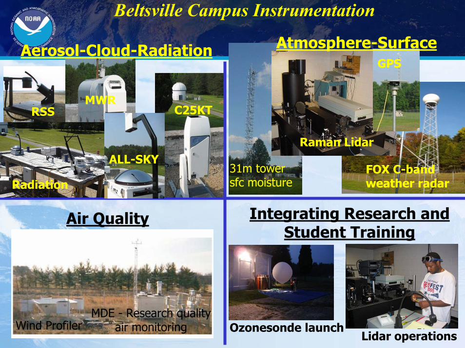
Beltsville Campus Instrumentation

RSS

31m towersfc moisture

Raman Lidar

FOX C-band weather radar

MWRC25KT

Radiation

Aerosol-Cloud-Radiation

ALL-SKY

Atmosphere-SurfaceGPS

Integrating Research andStudent Training

Air Quality

MDE - Research quality air monitoringWind Profiler

Lidar operationsOzonesonde launch

28

Conversion of species from one pressure grid to another needs to be done correctly!

• Radiosondes measure water at specific levels (usually relative humidity). Usually 10’s of thousands of points are measured in a single assent.

• This can be converted to a mixing ratio at a given level; however, there can be a lot of vertical structure (moist or dry layers) that are beyond any remote sounding instruments capability to measure.

• When comparing measurements it is important to– Have a common vertical resolution– Conserve the molecules to be compared (don’t count

molecules twice).

29

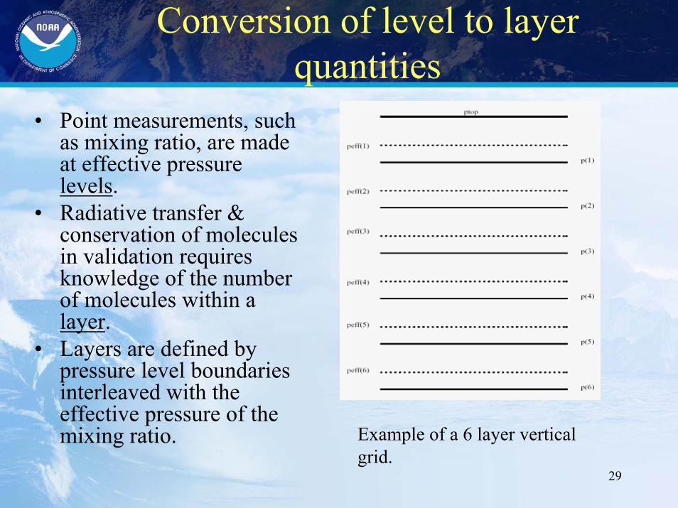
Conversion of level to layer quantities

• Point measurements, such as mixing ratio, are made at effective pressure levels.

• Radiative transfer & conservation of molecules in validation requires knowledge of the number of molecules within a layer.

• Layers are defined by pressure level boundaries interleaved with the effective pressure of the mixing ratio. Example of a 6 layer vertical

grid.

30

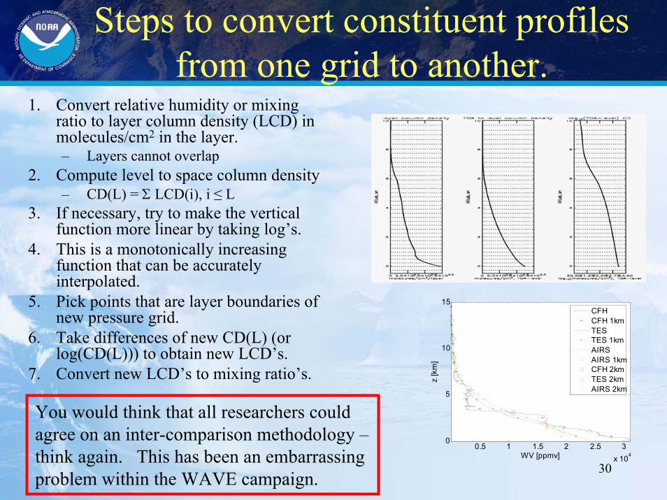
Steps to convert constituent profiles from one grid to another.

1. Convert relative humidity or mixing ratio to layer column density (LCD) in molecules/cm2 in the layer.– Layers cannot overlap

2. Compute level to space column density– CD(L) = Σ LCD(i), i ≤ L

3. If necessary, try to make the vertical function more linear by taking log’s.

4. This is a monotonically increasing function that can be accurately interpolated.

5. Pick points that are layer boundaries of new pressure grid.

6. Take differences of new CD(L) (or log(CD(L))) to obtain new LCD’s.

7. Convert new LCD’s to mixing ratio’s.

0.5 1 1.5 2 2.5 3x 104

0

5

10

15

z [k

m]

WV [ppmv]

CFHCFH 1kmTESTES 1kmAIRSAIRS 1kmCFH 2kmTES 2kmAIRS 2km

You would think that all researchers could agree on an inter-comparison methodology –think again. This has been an embarrassing problem within the WAVE campaign.

31

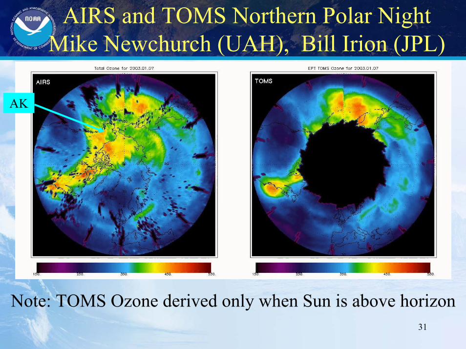
AIRS and TOMS Northern Polar NightMike Newchurch (UAH), Bill Irion (JPL)

AK

Note: TOMS Ozone derived only when Sun is above horizon

32

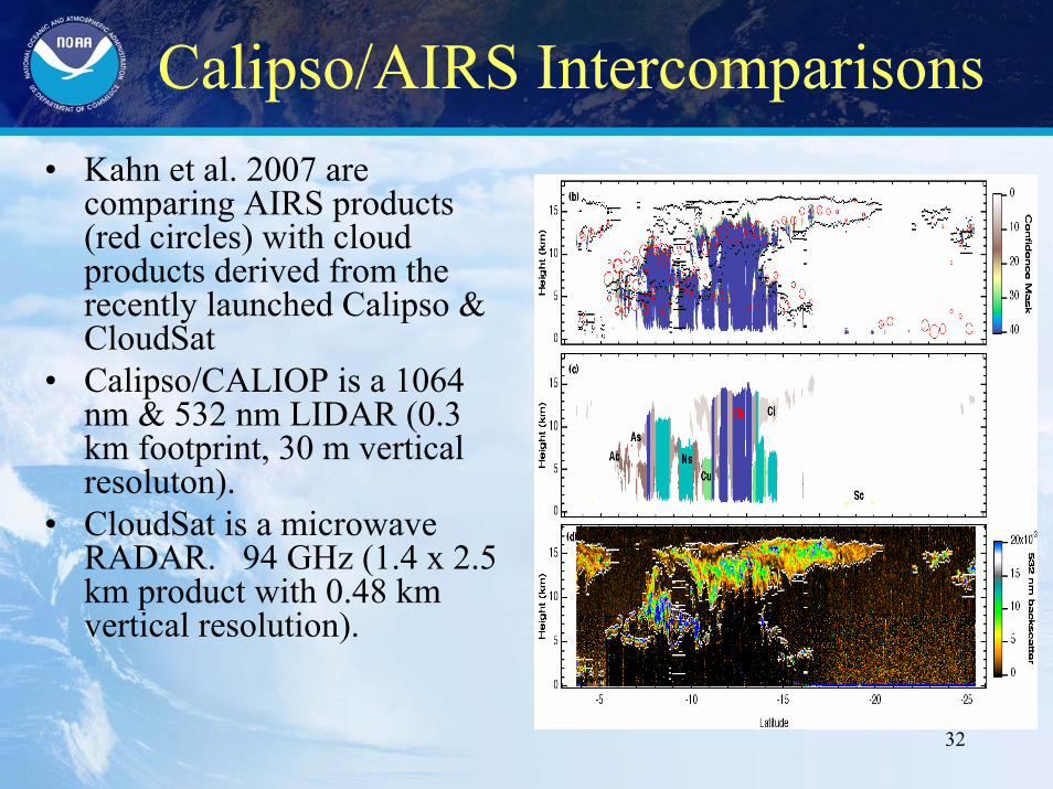
Calipso/AIRS Intercomparisons• Kahn et al. 2007 are

comparing AIRS products (red circles) with cloud products derived from the recently launched Calipso & CloudSat

• Calipso/CALIOP is a 1064 nm & 532 nm LIDAR (0.3 km footprint, 30 m vertical resoluton).

• CloudSat is a microwave RADAR. 94 GHz (1.4 x 2.5 km product with 0.48 km vertical resolution).

33

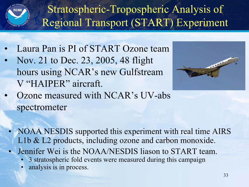
Stratospheric-Tropospheric Analysis of Regional Transport (START) Experiment

• Laura Pan is PI of START Ozone team• Nov. 21 to Dec. 23, 2005, 48 flight

hours using NCAR’s new GulfstreamV “HAIPER” aircraft.

• Ozone measured with NCAR’s UV-abs spectrometer

• NOAA NESDIS supported this experiment with real time AIRS L1b & L2 products, including ozone and carbon monoxide.

• Jennifer Wei is the NOAA/NESDIS liason to START team.• 3 stratospheric fold events were measured during this campaign • analysis is in process.

34

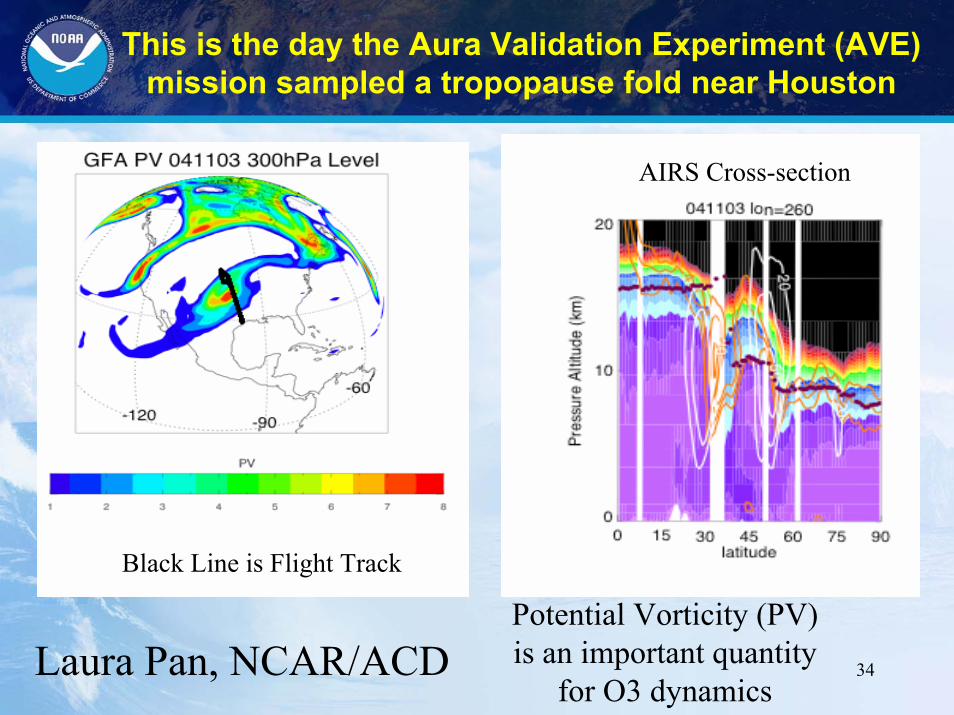
This is the day the Aura Validation Experiment (AVE) mission sampled a tropopause fold near Houston

AIRS Cross-section

Potential Vorticity (PV) is an important quantity

for O3 dynamics

Black Line is Flight Track

Laura Pan, NCAR/ACD

35

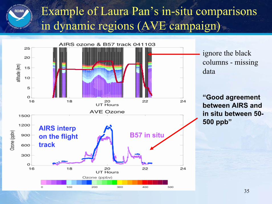
Example of Laura Pan’s in-situ comparisons in dynamic regions (AVE campaign)

AIRS interpon the flight track

B57 in situ

ignore the black columns - missing data

“Good agreement between AIRS and in situ between 50-500 ppb”

36

Movies• WAVES_Launch_18July.avi

– RS-92/Ozonesonde launch on July 18, 2006 from Beltsville MD.• AIRS_AGU_video v2_720x480.mov

– “Probably the best water vapor dataset available.” Andrew Dessler

– “The AIRS data is a key link in providing observations at prettymuch unprecedented spatial and time scales over regions of the planet where we have never had observations of the planet before.” Andrew Gettelman

– “AIRS is really the first global satellite dataset that has a very high quality, both water vapor and ozone, in both data quality and spatial/temporal resolution that can contribute in tropopauseregions.” Laura Pan

37

Atmospheric Carbon Retrievals

1.Brief introduction to all AIRS/IASI trace gas products.

2.Show example of AIRS CO2 product.

38

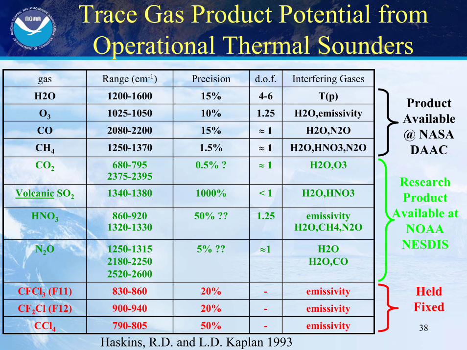
Trace Gas Product Potential from Operational Thermal Sounders

Haskins, R.D. and L.D. Kaplan 1993emissivity-50%790-805CCl4

emissivity-20%900-940CF2Cl (F12)

emissivity-20%830-860CFCl3 (F11)

H2OH2O,CO

≈15% ??1250-13152180-22502520-2600

N2O

emissivityH2O,CH4,N2O

1.2550% ??860-9201320-1330

HNO3

H2O,HNO3< 11000%1340-1380Volcanic SO2

H2O,O3≈ 10.5% ?680-7952375-2395

CO2

H2O,HNO3,N2O≈ 11.5%1250-1370CH4

H2O,N2O≈ 115%2080-2200CO

H2O,emissivity1.2510%1025-1050O3

T(p)4-615%1200-1600H2O

Interfering Gasesd.o.f.PrecisionRange (cm-1)gas

ProductAvailable@ NASA

DAAC

Research Product

Available at NOAA

NESDIS

Held Fixed

39

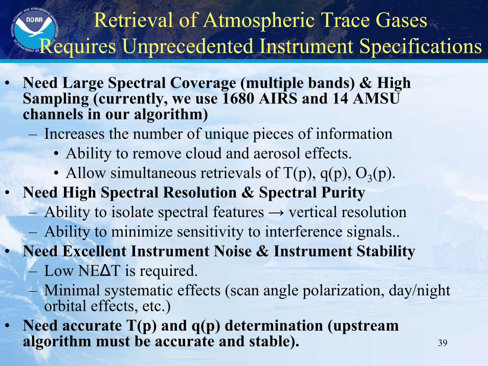
Retrieval of Atmospheric Trace GasesRequires Unprecedented Instrument Specifications

• Need Large Spectral Coverage (multiple bands) & High Sampling (currently, we use 1680 AIRS and 14 AMSU channels in our algorithm)– Increases the number of unique pieces of information

• Ability to remove cloud and aerosol effects.• Allow simultaneous retrievals of T(p), q(p), O3(p).

• Need High Spectral Resolution & Spectral Purity– Ability to isolate spectral features → vertical resolution– Ability to minimize sensitivity to interference signals..

• Need Excellent Instrument Noise & Instrument Stability– Low NE∆T is required.– Minimal systematic effects (scan angle polarization, day/night

orbital effects, etc.) • Need accurate T(p) and q(p) determination (upstream

algorithm must be accurate and stable).

40

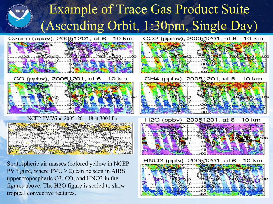
Example of Trace Gas Product Suite(Ascending Orbit, 1:30pm, Single Day)

NCEP PV/Wind 20051201_18 at 300 hPa

Stratospheric air masses (colored yellow in NCEP PV figure, where PVU ≥ 2) can be seen in AIRS upper tropospheric O3, CO, and HNO3 in the figures above. The H2O figure is scaled to show tropical convective features.

41

Utility of Trace Gas Correlations

• To identify interesting dynamical regimes for scientific study.– Identify regions of atmospheric stratospheric/tropospheric

exchange (STE)– Identify source regions of trace gases (e.g., biomass burning,

pollution).– Identify regions of interesting transport (e.g., Brewer Dobson

circulation of CH4 and CO2) or photochemistry (e.g., O3 production from CO).

• A diagnostic tool to help improve satellite measurements of trace gases

• Problems in specific situations (e.g., deserts, topography, isothermal)• Improper spectral separation of gases (e.g., HNO3/CH4)

42

29 month time-series of AIRS productsSouth America Zone (-25 ≤ lat ≤ EQ , -70 ≤ lon ≤ -40)

43

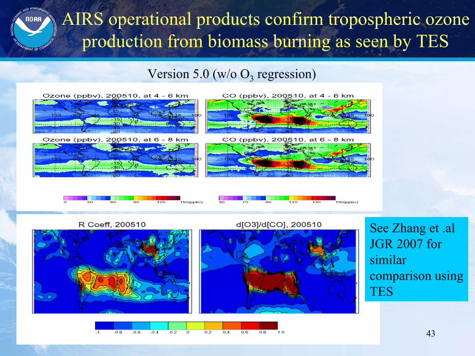
AIRS operational products confirm tropospheric ozone production from biomass burning as seen by TES

Version 5.0 (w/o O3 regression)

See Zhang et .al JGR 2007 for similar comparison using TES

44

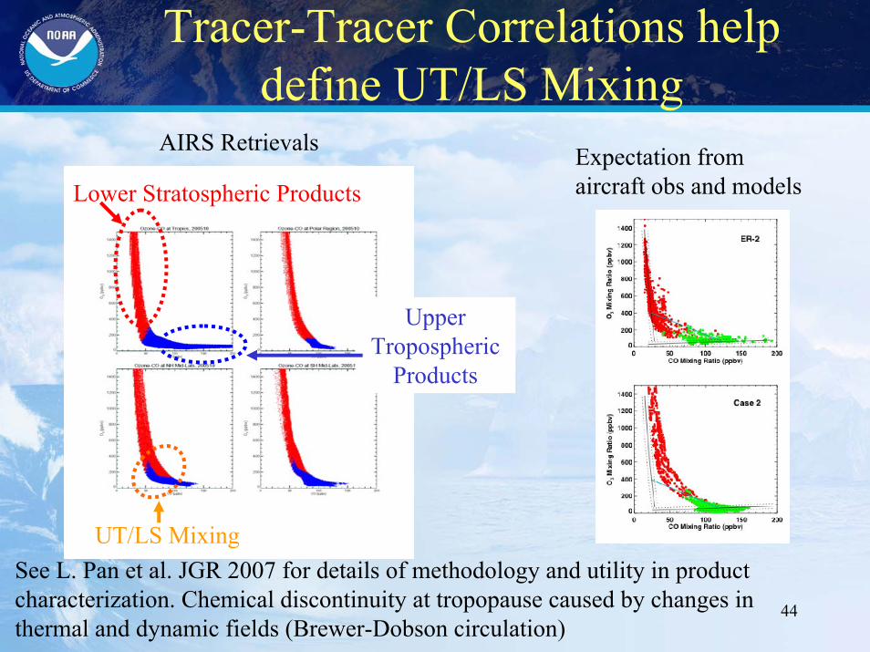
Tracer-Tracer Correlations help define UT/LS Mixing

See L. Pan et al. JGR 2007 for details of methodology and utility in product characterization. Chemical discontinuity at tropopause caused by changes in thermal and dynamic fields (Brewer-Dobson circulation)

UT/LS Mixing

Lower Stratospheric Products

Upper Tropospheric

Products

Expectation from aircraft obs and models

AIRS Retrievals

45

Motivation for Carbon Trace Gases

• Fossil fuel emissions are rapidly increasing the amount of atmospheric carbon dioxide (CO2) that results in a increase in the energy of the atmosphere.– Understanding sources and sinks of atmospheric CO2 and the transport and

lifetime in the atmosphere is a critical component of understanding climate change.

• Atmospheric methane (CH4) has a larger climate impact– Quantifying emissions from wetlands, agriculture, landfills, fires, etc. is

important to understanding the atmospheric concentration.– Regulating methane emissions could mitigate a significant portion of the

anthropogenic climate impact.– Rapid warming in polar regions has the potential of a large positive feedback

due to melting of Pleistocene-age ices and rapid emissions of large amounts of CH4

• Carbon monoxide (CO) and ozone (O3) can help distinguish sources and of atmospheric carbon and characterize transport.

46

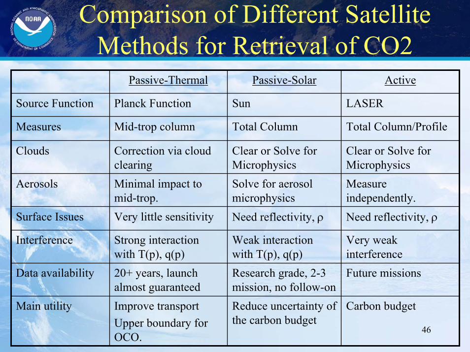
Comparison of Different Satellite Methods for Retrieval of CO2

Measure independently.

Solve for aerosol microphysics

Minimal impact to mid-trop.

Aerosols

Main utility

Data availability

Interference

Surface Issues

Clouds

Measures

Source Function

Carbon budgetReduce uncertainty of the carbon budget

Improve transportUpper boundary for OCO.

Future missionsResearch grade, 2-3 mission, no follow-on

20+ years, launch almost guaranteed

Very weak interference

Weak interaction with T(p), q(p)

Strong interaction with T(p), q(p)

Need reflectivity, ρNeed reflectivity, ρVery little sensitivity

Clear or Solve for Microphysics

Clear or Solve for Microphysics

Correction via cloud clearing

Total Column/ProfileTotal ColumnMid-trop column

LASERSunPlanck Function

ActivePassive-SolarPassive-Thermal

47

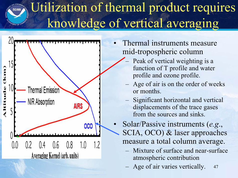
Utilization of thermal product requires knowledge of vertical averaging

• Thermal instruments measure mid-tropospheric column– Peak of vertical weighting is a

function of T profile and water profile and ozone profile.

– Age of air is on the order of weeks or months.

– Significant horizontal and vertical displacements of the trace gases from the sources and sinks.

• Solar/Passive instruments (e.g., SCIA, OCO) & laser approaches measure a total column average.– Mixture of surface and near-surface

atmospheric contribution– Age of air varies vertically.

48

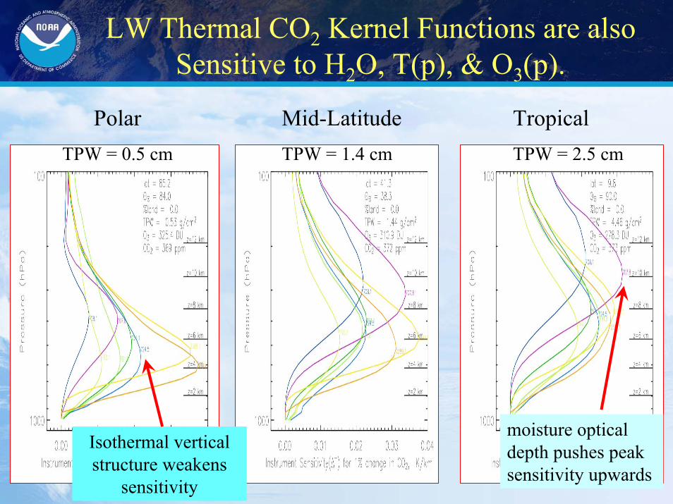
LW Thermal CO2 Kernel Functions are also Sensitive to H2O, T(p), & O3(p).

Mid-LatitudeTPW = 1.4 cm

PolarTPW = 0.5 cm

Isothermal vertical structure weakens

sensitivity

TropicalTPW = 2.5 cm

moisture optical depth pushes peak sensitivity upwards

49

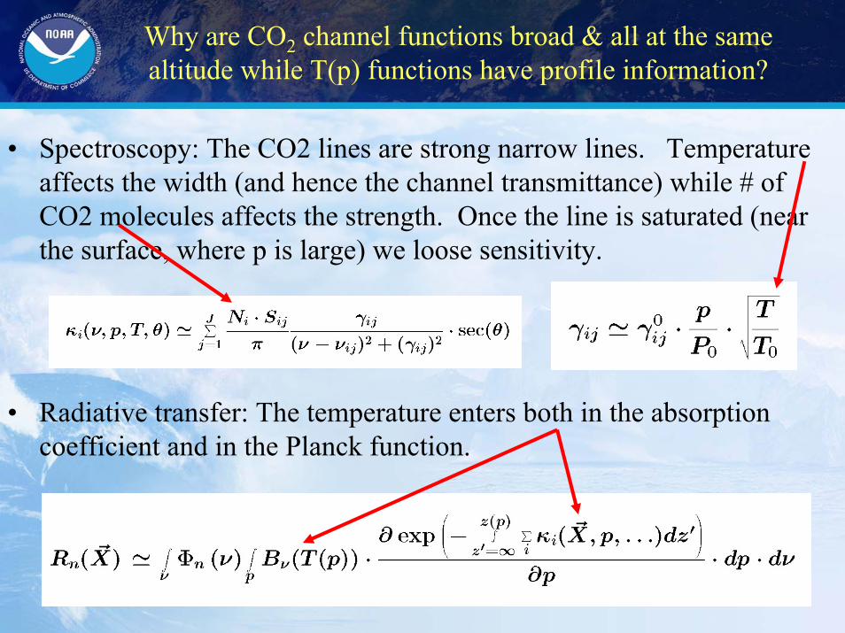
Why are CO2 channel functions broad & all at the same altitude while T(p) functions have profile information?

• Spectroscopy: The CO2 lines are strong narrow lines. Temperature affects the width (and hence the channel transmittance) while # of CO2 molecules affects the strength. Once the line is saturated (near the surface, where p is large) we loose sensitivity.

• Radiative transfer: The temperature enters both in the absorption coefficient and in the Planck function.

50

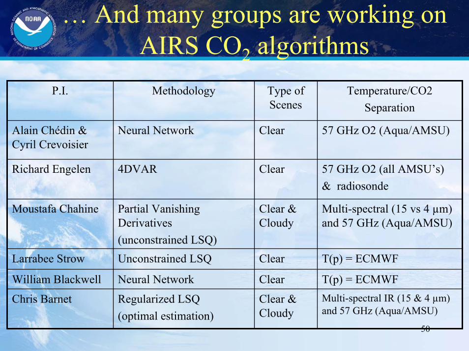
… And many groups are working on AIRS CO2 algorithms

T(p) = ECMWFClearUnconstrained LSQLarrabee Strow

Temperature/CO2Separation

Type of Scenes

MethodologyP.I.

Clear & Cloudy

Clear

Clear & Cloudy

Clear

Clear

Multi-spectral IR (15 & 4 µm) and 57 GHz (Aqua/AMSU)

Regularized LSQ(optimal estimation)

Chris Barnet

T(p) = ECMWFNeural NetworkWilliam Blackwell

Multi-spectral (15 vs 4 µm) and 57 GHz (Aqua/AMSU)

Partial Vanishing Derivatives(unconstrained LSQ)

Moustafa Chahine

57 GHz O2 (all AMSU’s)& radiosonde

4DVARRichard Engelen

57 GHz O2 (Aqua/AMSU)Neural NetworkAlain Chédin & Cyril Crevoisier

51

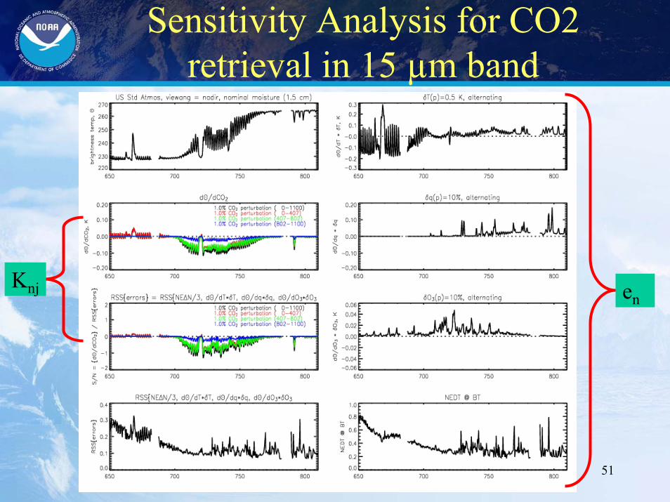
Sensitivity Analysis for CO2 retrieval in 15 µm band

Knj en

52

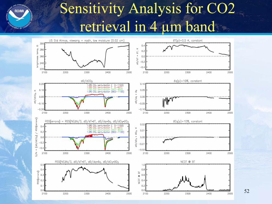
Sensitivity Analysis for CO2 retrieval in 4 µm band

53

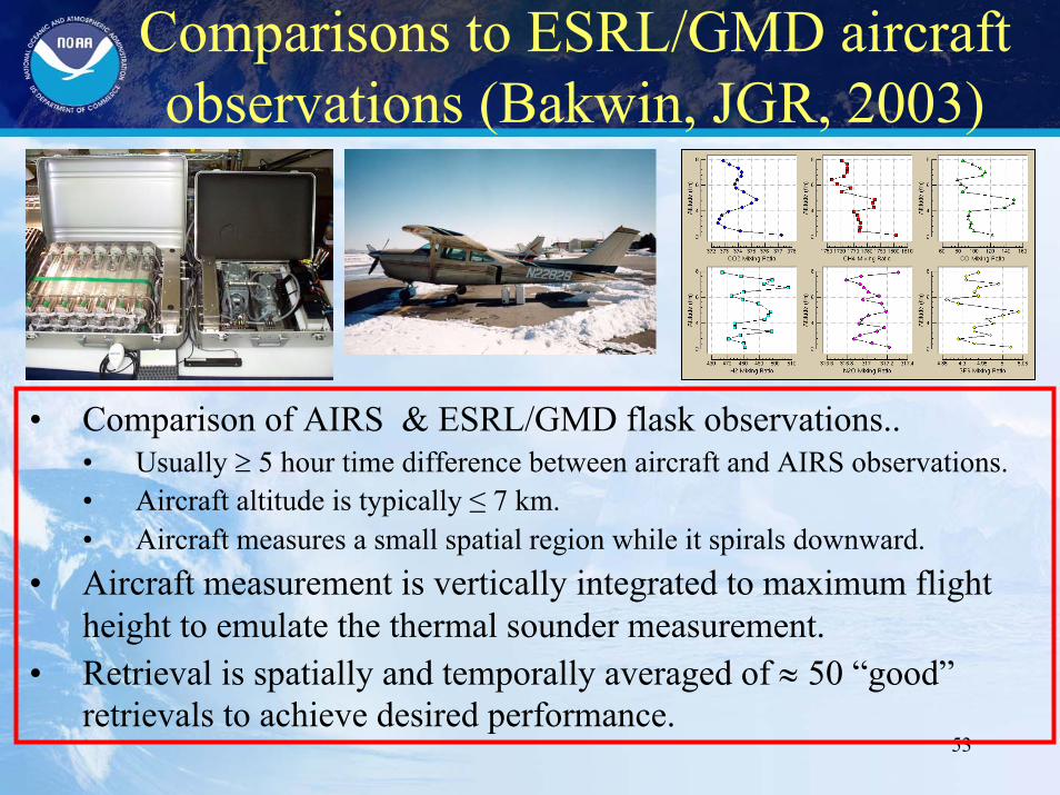
Comparisons to ESRL/GMD aircraft observations (Bakwin, JGR, 2003)

• Comparison of AIRS & ESRL/GMD flask observations..• Usually ≥ 5 hour time difference between aircraft and AIRS observations.• Aircraft altitude is typically ≤ 7 km.• Aircraft measures a small spatial region while it spirals downward.

• Aircraft measurement is vertically integrated to maximum flight height to emulate the thermal sounder measurement.

• Retrieval is spatially and temporally averaged of ≈ 50 “good” retrievals to achieve desired performance.

54

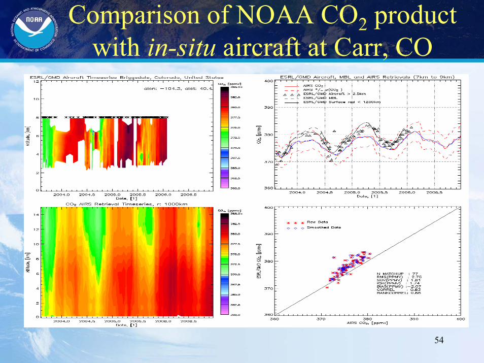
Comparison of NOAA CO2 product with in-situ aircraft at Carr, CO

55

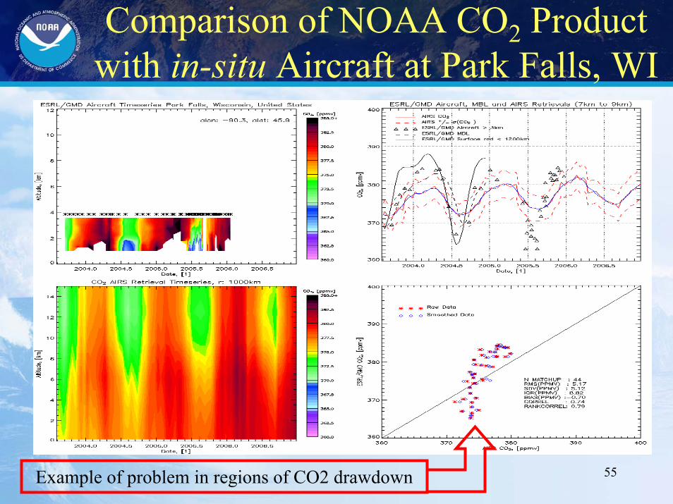
Comparison of NOAA CO2 Product with in-situ Aircraft at Park Falls, WI

Example of problem in regions of CO2 drawdown

56

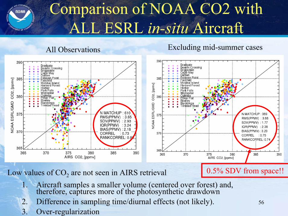
Comparison of NOAA CO2 with ALL ESRL in-situ Aircraft

Excluding mid-summer casesAll Observations

0.5% SDV from space!!Low values of CO2 are not seen in AIRS retrieval1. Aircraft samples a smaller volume (centered over forest) and,

therefore, captures more of the photosynthetic drawdown2. Difference in sampling time/diurnal effects (not likely).3. Over-regularization

57

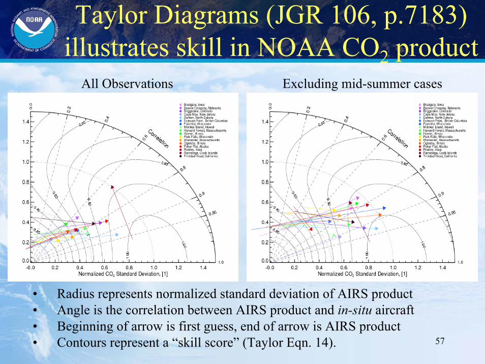
Taylor Diagrams (JGR 106, p.7183) illustrates skill in NOAA CO2 product

All Observations Excluding mid-summer cases

• Radius represents normalized standard deviation of AIRS product• Angle is the correlation between AIRS product and in-situ aircraft• Beginning of arrow is first guess, end of arrow is AIRS product• Contours represent a “skill score” (Taylor Eqn. 14).

58

NOAA AIRS CO2 Product is Still in Development

• Measuring a product to 0.5% is inherently difficult– Empirical bias correction (a.k.a. tuning) for AIRS is at the 1 K level and can

affect the CO2 product.– Errors in moisture of ±10% is equivalent to ±0.7 ppmv errors in CO2.– Errors in surface pressure of ±5 mb induce ±1.8 ppmv errors in CO2.– AMSU side-lobe errors minimize the impact of the 57 GHZ O2 band as a T(p)

reference point.– Bottom Line: Core product retrieval problems must be solved first.

• Currently, we can characterize seasonal and latitudinal mid-tropospheric variability to test product reasonableness.

• The real questions is whether thermal sounders can contribute to the source/sink questions.– Requires accurate vertical & horizontal transport models – Having simultaneous O3, CO, CH4, and CO2 products is a unique contribution

that thermal sounders can make to improve the understanding of transport.

59

So maybe the utility of thermal sounders has yet to be exploited

• AIRS has produces the first global tropospheric measurement of CO2 & CH4.

• AIRS, IASI, and CrIS should provide a long-term dataset.• AIRS has a unique capability to inter-compare tropospheric

products of temperature, water, O3, CO, CH4, and CO2.• We expect to learn new things from this dataset.• We are exploring diurnal signals and hope to identify large

pollution or biosphere events over the lifetime of these instruments.• We are exploring the use of trace gas correlations within the AIRS

products as an analysis to help identify sources of trace gases.• We want to work with transport modelers to compare our product

to a realistic emission scenario for CO2 with proper vertical weighing functions.

• Other ideas?

60

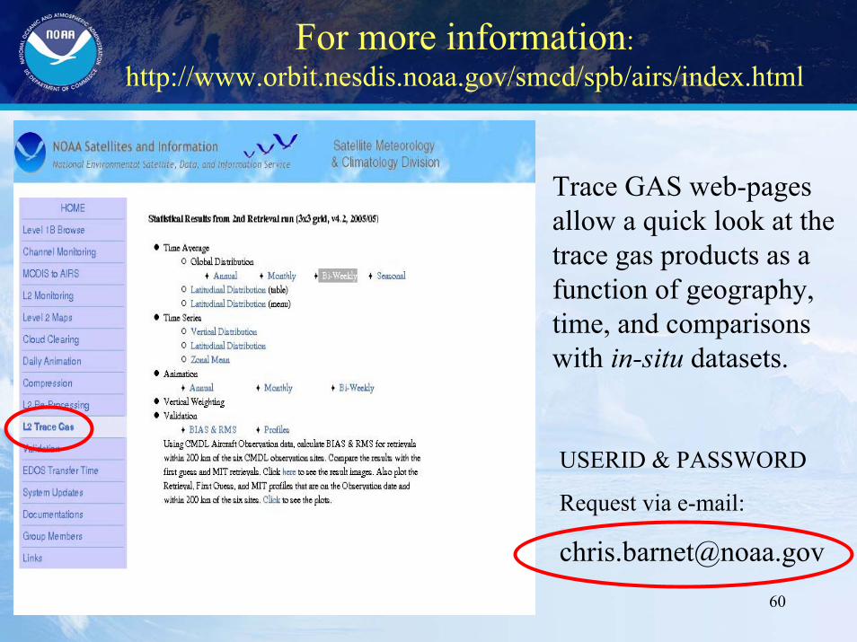
For more information:http://www.orbit.nesdis.noaa.gov/smcd/spb/airs/index.html

• Trace GAS web-pages allow a quick look at the trace gas products as a function of geography, time, and comparisons with in-situ datasets.

USERID & PASSWORD

Request via e-mail:

chris.barnet@noaa.gov

61

Some ReferencesAIRS Instrument & Retrieval Algorithms

• Aumann, H.H., M.T. Chahine, C. Gautier, M.D. Goldberg, E. Kalnay, L.M. McMillin, H. Revercomb, P.W. Rosenkranz, W.L. Smith, D.H. Staelin, L.L. Strow and J. Susskind 2003. AIRS/AMSU/HSB on the Aqua mission: design, science objectives, data products, and processing systems. IEEE Trans. Geosci. Remote Sens. 41 p.253- 264.

• Barnet, C.D., M. Goldberg, L. McMillin, E.S. Maddy and M.T. Chahine 2005. Remote sounding of trace gases from advanced sounders. FTS/HISE, OSA Technical Digest (Optical Soc. Amer.) 3 pgs. (paper HMC3)

• Barnet, C.D., M. Goldberg, L.M. McMillin and M.T. Chahine 2004. Remote sounding of trace gases with the EOS/AIRS instrument. SPIE 5548 p.300-312.

• Barnet, C.D., S. Datta and L. Strow 2003. Trace gas measurements from the atmospheric infrared sounder (AIRS). Optical Remote Sensing, OSA Technical Digest p.89-92.

• Chahine, M.T., C.D. Barnet, E.T. Olsen, L. Chen and E. Maddy 2005. On the determination of atmospheric minor gases by the method of vanishing partial derivatives with application to CO2. Geophys. Res. Lett. 32 L22803 doi:10.1029/2005GL0241651, 5 pgs.

• Goldberg, M.D., Y. Qu, L.M. McMillin, W.W. Wolf, L. Zhou and M. Divakarla 2003. AIRS near-real-time products and algorithms in support of operational weather prediction. IEEE Trans. Geosci. Remote Sens. 41 p.379-389.

• Maddy, E.S., C.D. Barnet, L.M. McMillin, M. Goldberg and M.T. Chahine 2005. Investigating the separability of temperature and CO2 from operational hyper-spectral sounders. FTS/HISE, OSA Technical Digest (Optical Soc. Amer.) 3 pgs. (paper HTuD10)

• Rodgers, C.D. 2000. Inverse methods for atmospheric sounding: Theory and practice. World Scientific Publishing 238 pgs.

• Rodgers, C.D. and B.J. Conner 2003. Inter-comparison of remote sounding instruments. J. Geophys. Res. v.108 p.1-14. doi:10.1029/2002JD002299

62

Sample ReferencesValidation

• Divakarla, M.G., C.D. Barnet, M.D. Goldberg, L.M. McMillin, E. Maddy, W.W. Wolf, L. Zhou and X. Liu 2006. Validation of Atmospheric Infrared Sounder temperature and water vapor retrievals with matched radiosonde measurements and forecasts. J. Geophys. Res. v.111 D09S15 doi:10.1029/2005JD006116, 20 pgs.

• Eskridge, R.E., J.K. Luers and C.R. Redder 2003. Unexplained Discontinuity in the U.S. RadiosondeTemperature Data. Part I: Troposphere. J. Climate v.16 p.2385-2395.

• Gettelman, A., E.M. Weinstock, E.J. Fetzer, F.W. Irion, A. Eldering, E.C. Richard, K.H. Rosenlof, T.L. Thompson, J.V. Pittman, C.R. Webster and R.L. Herman 2004. Validation of Aqua satellite data in the upper troposphere and lower stratosphere with in situ aircraft. Geophys. Res. Lett. v.31 L22107 doi:10.1029/2004GL020730

• Kahn, B.H., M. T. Chahine, G. L. Stephens, G. G. Mace, R. T. March, and Z. Wang, A. Eldering, R. E. Holz, R. E. Kuehn, D.G. Vane and C. D. Barnet 2007. Cloud type comparisons of AIRS, CloudSat, and CALIPSO cloud height and amount. Submitted to Atmos. Chem. Phys.

• Kawa, S.R, D.J. Erickson III, S. Pawson and Z. Shu 2004. Global CO2 transport simulations using meteorological data from the NASA data assimilation system. J. Geophys. Res. v.109 D18312 doi:10.1029/2004J004 554, 17 pgs.

• Pan, L., K.P. Bowman, M. Shapiro, W.J. Randel, R. Gao, T. Campos, A. Cooper, C. Davis, S. Schauffler, B.A. Ridley, J.C. Wei and C. Barnet 2007. Chemical behavior of the tropopause observed during the Stratosphere-Troposphere Analyses of Regional Transport (START) experiment. J. Geophys. Res. In press

• Taylor, K.E. 2001. Summarizing multiple aspects of model performance in a single diagram. J. Geophys. Res. v.106 p.7183-7192. doi:10.1029/2000JD900719

• Tobin, D.C., H.E. Revercomb, C.C. Moeller and T.S. Pagano 2006. Use of Atmospheric Infrared Sounder high spectral resolution spectra to assess the calibration of Moderate resolution Imaging Spectroradiometer on EOS Aqua. J. Geophys. Res. v.111 D09S05 doi:10.1029/2005JD006095, 15 pgs.

• Tobin, D.C., H.E. Revercomb, R.O. Knuteson, B.L. Lesht, L.L. Strow, S.E. Hannon, W.F. Feltz, L.A. Moy, E.J. Fetzer and T.S. Cress 2006. Atmospheric Radiation Measurement site atmospheric state best estimates for Atmospheric Infrared Sounder temperature and water retrieval validation. J. Geophys. Res. v.111 D09S14 doi:10.1029/2005JD006103, 18 pgs.

63

ReferencesAIRS Trace Gas Algorithms

• Haskins, R.D. and L.D. Kaplan 1993. Remote sensing of trace gases using the atmospheric infrared sounder. Intl Rad. Symp. (QC912.3 I57 1992, Deepak Publ.) p.278-281.

• Crevoisier, C., S. Heilliette, A. Chedin, S. Serrar, R. Armante and N.A. Scott 2004. Midtropospheric CO2 concentration retrieval from AIRS observations in the tropics. Geophys. Res. Lett. v.31 p.17106-17110. doi:10.1029/2004GL020141

• Crevoisier, C., A. Chedin and N.A. Scott 2003. AIRS channels selection for CO2 and othertrace gases retrieval. Quart. J. Roy. Meteor. Soc. v.128 p.2719-2740. doi:10.1256/qj.02.180

• Engelen, R.J. and A.P. McNally 2005. Estimating atmospheric CO2 from advanced IR satellite radiances within an operational 4D-Var data assim. system: Results and Validation. J. Geophys. Res. v.110 D18305 doi:10.1029/2005JD005982

• Engelen, R.J. and G.L. Stephens 2004. Information content of infrared satellite sounding measurements with respect to CO2. J. Appl. Meteor. v.43 p.373-378.

• Engelen, R.J., G.L. Stephens and A.S. Denning 2001. The effect of CO2 variability on the retrieval of atmospheric temperatures. Geophys. Res. Lett. v.28 p.3259-3263.

64

Other ReferencesSTE & Gas Correlations

• Bakwin, P.S., P.P. Tans, B.B. Stephens, S.C. Wofsy, C. Grebig and A. Grainger 2003. Strategies for measurement of atmospheric column means of carbon dioxide from aircraft using discrete sampling. J. Geophys. Res. 108p.4514-4520.

• Matsueda, H., H.Y. Inoue and M. Ishii 2002. Aircraft observation of carbon dioxide at 8-13 km altitude over the western Pacific from 1993 to 1999. Tellus-B 54 p.1-21.

• Pan, L.L., J. C. Wei, D. E. Kinnison, R. R. Garcia, D. J. Wuebbles, and G. P. Brasseur 2007. A set of diagnostics for evaluating chemistry-climate models in the extratropical tropopause region. JGR, In-press

• Shia, R.L., M.C. Liang, C.E. Miller and Y.L. Yung 2006. CO2 in the upper troposphere: influence of stratosphere-troposphere exchange. Geophys. Res. Lett. 33 L14814 doi:10.1029/2006GL026141, 4 pgs.

• Zhang, L., D.J. Jacob, K.W. Bowman, J. A. Logan, Solène Turquety, R. C. Hudman, Q. Li, R. Beer, H. M. Worden, J. R. Worden, C. P. Rinsland, S. S. Kulawik, M. C. Lampel, M. W. Shephard, B. M. Fisher, A. Eldering, and M. A. Avery. 2007 Continental outflow of ozone pollution as determined by O3-CO correlations from the TES satellite instrument. JGR, in press.