Embed Size (px)
Citation preview
Optimization over Structured Subsets ofPositive Semidefinite Matrices via Column Generation
Amir Ali Ahmadi∗
Princeton, ORFEa a [email protected]
Sanjeeb DashIBM Research
Georgina Hall∗
Princeton, [email protected]
December 16, 2015
Abstract
We develop algorithms for inner approximating the cone of positive semidefinite matrices via linearprogramming and second order cone programming. Starting with an initial linear algebraic approxima-tion suggested recently by Ahmadi and Majumdar, we describe an iterative process through which ourapproximation is improved at every step. This is done using ideas from column generation in large-scalelinear and integer programming. We then apply these techniques to approximate the sum of squarescone in a nonconvex polynomial optimization setting, and the copositive cone for a discrete optimizationproblem.
1 Introduction
Semidefinite programming is a powerful tool in optimization that is used in many different contexts, perhapsmost notably to obtain strong bounds on discrete optimization problems or nonconvex polynomial programs.One difficulty in applying semidefinite programming is that state-of-the-art general-purpose solvers oftencannot solve very large instances reliably and in a reasonable amount of time. As a result, at relativelylarge scales, one has to resort either to specialized solution techniques and algorithms that employ problemstructure, or to easier optimization problems that lead to weaker bounds. We will focus on the latter approachin this paper.
At a high level, our goal is to not solve semidefinite programs (SDPs) to optimality, but rather replacethem with cheaper conic relaxations—linear and second order cone relaxations to be precise—that returnuseful bounds quickly. Throughout the paper, we will aim to find lower bounds (for minimization prob-lems); i.e., bounds that certify the distance of a candidate solution to optimality. Fast, good-quality lowerbounds are especially important in the context of branch-and-bound schemes, where one needs to strike adelicate balance between the time spent on bounding and the time spent on branching, in order to keep theoverall solution time low. Currently, in commercial integer programming solvers, almost all lower boundingapproaches using branch-and-bound schemes exclusively produce linear inequalities. Even though semidef-inite cuts are known to be stronger, they are often too expensive to be used even at the root node of a
∗Amir Ali Ahmadi and Georgina Hall are partially supported by the Young Investigator Program award of the AFSOR.
1
branch-and-bound tree. Because of this, many high-performance solvers, e.g., IBM ILOG CPLEX [15] andGurobi [1], do not even provide an SDP solver and instead solely work with LP and SOCP relaxations. Ourgoal in this paper is to offer some tools that exploit the power of SDP-based cuts, while staying entirelyin the realm of LP and SOCP. We apply these tools to classical problems in both nonconvex polynomialoptimization and discrete optimization.
Techniques that provide lower bounds on minimization problems are precisely those that certify non-negativity of objective functions on feasible sets. To see this, note that a scalar γ is a lower bound on theminimum value of a function f : Rn → R on a set K ⊆ Rn, if and only if f(x)− γ ≥ 0 for all x ∈ K. Asmost discrete optimization problems (including those in the complexity class NP) can be written as polyno-mial optimization problems, the problem of certifying nonnegativity of polynomial functions, either globallyor on basic semialgebraic sets, is a fundamental one. A polynomial p(x) := p(x1, . . . , xn) is said to be non-negative, if p(x) ≥ 0 for all x ∈ Rn. Unfortunately, even in this unconstrained setting, the problem of testingnonnegativity of a polynomial p is NP-hard even when its degree equals four. This is an immediate corollaryof the fact that checking if a symmetric matrix M is copositive—i.e., if xTMx ≥ 0, ∀x ≥ 0—is NP-hard.1
Indeed, M is copositive if and only if the homogeneous quartic polynomial p(x) =∑
i,jMi,jx2ix
2j is non-
negative.Despite this computational complexity barrier, there has been great success in using sum of squares
(SOS) programming [32], [22], [30] to obtain certificates of nonnegativity of polynomials in practical set-tings. It is known from Artin’s solution [7] to Hilbert’s 17th problem that a polynomial p(x) is nonnegativeif and only if
p(x) =
∑ti=1 q
2i (x)∑r
i=1 g2i (x)
⇔ (
r∑i=1
g2i (x))p(x) =
t∑i=1
q2i (x) (1)
for some polynomials q1, . . . , qt, g1, . . . , gr. When p is a quadratic polynomial, then the polynomials gi arenot needed and the polynomials qi can be assumed to be linear functions. In this case, by writing p(x) as
p(x) =
(1
x
)TQ
(1
x
),
where Q is an (n+ 1)× (n+ 1) symmetric matrix, checking nonnegativity of p(x) reduces to checking thenonnegativity of the eigenvalues of Q; i.e., checking if Q is positive semidefinite.
More generally, if the degrees of qi and gi are fixed in (1), then checking for a representation of p ofthe form in (1) reduces to solving an SDP, whose size depends on the dimension of x, and the degreesof p, qi and gi [32]. This insight has led to significant progress in certifying nonnegativity of polynomialsarising in many areas. In practice, the “first level” of the SOS hierarchy is often the one used, where thepolynomials gi are left out and one simply checks if p is a sum of squares of other polynomials. In this casealready, because of the numerical difficulty of solving large SDPs, the polynomials that can be certified tobe nonnegative usually do not have very high degrees or very many variables. For example, finding a sum ofsquares certificate that a given quartic polynomial over n variables is nonnegative requires solving an SDPinvolving roughly O(n4) constraints and a positive semidefinite matrix variable of size O(n2) × O(n2).Even for a handful of or a dozen variables, the underlying semidefinite constraints prove to be expensive.Indeed, in the absence of additional structure, most examples in the literature have less than 10 variables.
1Weak NP-hardness of testing matrix copositivity is originally proven by Murty and Kabadi [29]; its strong NP-hardness isapparent from the work of de Klerk and Pasechnik [17].
2
Recently other systematic approaches to certifying nonnegativity of polynomials have been proposedwhich lead to less expensive optimization problems than semidefinite programming problems. In particu-lar, Ahmadi and Majumdar [4], [3] introduce “DSOS and SDSOS” optimization techniques, which replacesemidefinite programs arising in the nonnegativity certification problem by linear programs and second-order cone programs. Instead of optimizing over the cone of sum of squares polynomials, the authorsoptimize over two subsets which they call “diagonally dominant sum of squares” and “scaled diagonallydominant sum of squares” polynomials (see Section 2.1 for formal definitions). In the language of semidef-inite programming, this translates to solving optimization problems over the cone of diagonally dominantmatrices and scaled diagonally dominant matrices. These can be done by LP and SOCP respectively. Theauthors have had notable success with these techniques in different applications. For instance, they are ableto run these relaxations for polynomial optimization problems of degree 4 in 70 variables in the order of afew minutes. They have also used their techniques to push the size limits of some SOS problems in controls;examples include stabilizing a model of a humanoid robot with 30 state variables and 14 control inputs [26],or exploring the real-time applications of SOS techniques in problems such as collision-free autonomousmotion planning [5].
Motivated by these results, our goal in this paper is to start with DSOS and SDSOS techniques andimprove on them. By exploiting ideas from column generation in integer/linear programming, and by ap-propriately interpreting the DSOS and SDSOS constraints, we produce several iterative LP and SOCP-basedalgorithms that improve the quality of the bounds obtained from the DSOS and SDSOS relaxations. Geomet-rically, this amounts to optimizing over structured subsets of sum of squares polynomials that are larger thanthe sets of diagonally dominant or scaled diagonally dominant sum of squares polynomials. For semidefiniteprogramming, this is equivalent to optimizing over structured subsets of the cone of positive semidefinitematrices. An important distinction to make between the DSOS/SDSOS/SOS approaches and our approach,is that our approximations iteratively get larger in the direction of the given objective function, unlike theDSOS, SDSOS, and SOS approaches which all try to inner approximate the set of nonnegative polynomialsirrespective of any particular direction.
The organization of the rest of the paper is as follows. In the next section, we review relevant notation,and discuss the prior literature on DSOS and SDSOS programming. In Section 3, we give a high-leveloverview of our column generation approaches in the context of a general SDP. In Section 4, we describean application of our ideas to nonconvex polynomial optimization and present computational experimentswith certain column generation implementations. In Section 5, we apply our column generation approachto a specific discrete optimization application, namely the stable set problem. All the work in these sectionscan be viewed as providing techniques to optimize over subsets of positive semidefinite matrices. We thenconclude in Section 6 with some future directions, and discuss ideas for column generation which allow oneto go beyond subsets of positive semidefinite matrices in the case of polynomial optimization and the stableset problem.
2 Preliminaries
Let us first introduce some notation on matrices. We denote the set of real symmetric n × n matrices bySn. Given two matrices A and B in Sn, we denote their matrix inner product by A · B :=
∑i,j AijBij =
Trace(AB). The set of symmetric matrices with nonnegative entries is denoted byNn. A symmetric matrixA is positive semidefinite (psd) if xTAx ≥ 0 for all x ∈ Rn; this will be denoted by the standard notation
3
A � 0, and our notation for the set of n× n psd matrices is Pn. A matrix A is copositive if xTAx ≥ 0 forall x ≥ 0. The set of copositive matrices is denoted by Cn. All three sets Nn, Pn, Cn are convex cones andwe have the obvious inclusion Nn + Pn ⊆ Cn. This inclusion is strict if n ≥ 5 [13], [12]. For a cone ofmatrices in Sn, we define its dual cone K∗ as {Y ∈ Sn : Y ·X ≥ 0, ∀X ∈ K}.
For a vector variable x ∈ Rn and a vector q ∈ Zn+, let a monomial in x be denoted as xq := Πni=1x
qii ,
and let its degree be∑n
i=1 qi. A polynomial is said to be homogeneous or a form if all of its monomialshave the same degree. A form p(x) in n variables is nonnegative if p(x) ≥ 0 for all x ∈ Rn, or equivalentlyfor all x on the unit sphere in Rn. The set of nonnegative (or positive semidefinite) forms in n variablesand degree d is denoted by PSDn,d. A form p(x) is a sum of squares (sos) if it can be written as p(x) =∑r
i=1 q2i (x) for some forms q1, . . . , qr. The set of sos forms in n variables and degree d is a cone denoted
by SOSn,d. We have the obvious inclusion SOSn,d ⊆ PSDn,d, which is strict unless d = 2, or n = 2, or(n, d) = (3, 4) [20]. Let z(x, d) be the vector of all monomials of degree exactly d; it is well known that aform p of degree 2d is sos if and only if it can be written as p(x) = zT (x, d)Qz(x, d), for some psd matrixQ [32], [31]. The size of the matrix Q, which is often called the Gram matrix, is
(n+d−1
d
)×(n+d−1
d
). At
the price of imposing a semidefinite constraint of this size, one obtains the very useful ability to search andoptimize over the convex cone of sos forms via semidefinite programming.
2.1 DSOS and SDSOS optimization
In order to alleviate the problem of scalability posed by the SDPs arising from sum of squares programs, Ah-madi and Majumdar [4], [3]2 recently introduced similar-purpose LP and SOCP-based optimization prob-lems that they refer to as DSOS and SDSOS programs. Since we will be building on these concepts, webriefly review their relevant aspects to make our paper self-contained.
The idea in [4], [3] is to replace the condition that the Gram matrix Q be positive semidefinite withstronger but cheaper conditions in the hope of obtaining more efficient inner approximations to the coneSOSn,d. Two such conditions come from the concepts of diagonally dominant and scaled diagonally dom-inant matrices in linear algebra. We recall these definitions below.
Definition 2.1. A symmetric matrix A = (aij) is diagonally dominant (dd) if aii ≥∑
j 6=i |aij | for all i. Wesay that A is scaled diagonally dominant (sdd) if there exists a diagonal matrix D, with positive diagonalentries, such that DAD is diagonally dominant.
We refer to the set of n × n dd (resp. sdd) matrices as DDn (resp. SDDn). The following inclusionsare a consequence of Gershgorin’s circle theorem:
DDn ⊆ SDDn ⊆ Pn.
We now use these matrices to introduce the cones of “dsos” and “sdsos” forms and some of their gen-eralizations, which all constitute special subsets of the cone of nonnegative forms. We remark that in theinterest of brevity, we do not give the original definitions of dsos and sdsos polynomials as they appear in [4](as sos polynomials of a particular structure), but rather an equivalent characterization of them that is moreuseful for our purposes. The equivalence is proven in [4].
2The work in [4] is currently in preparation for submission; the one in [3] is a shorter conference version of [4] which hasalready appeared. The presentation of the current paper is meant to be self-contained.
4
Definition 2.2 ([3, 4]). Recall that z(x, d) denotes the vector of all monomials of degree exactly d. A formp(x) of degree 2d is said to be
• diagonally-dominant-sum-of-squares (dsos) if it admits a representation asp(x) = zT (x, d)Qz(x, d), where Q is a dd matrix.
• scaled-diagonally-dominant-sum-of-squares (sdsos) if it admits a representation asp(x) = zT (x, d)Qz(x, d), where Q is an sdd matrix.
• r-diagonally-dominant-sum-of-squares (r-dsos) if there exists a positive integer r such thatp(x)(
∑ni=1 x
2i )r is dsos.
• r-scaled diagonally-dominant-sum-of-squares (r-sdsos) if there exists a positive integer r such thatp(x)(
∑ni=1 x
2i )r is sdsos.
We denote the cone of forms in n variables and degree d that are dsos, sdsos, r-dsos, and r-sdsos byDSOSn,d, SDSOSn,d, rDSOSn,d, and rSDSOSn,d respectively. The following inclusion relations arestraightforward:
DSOSn,d ⊆ SDSOSn,d ⊆ SOSn,d ⊆ PSDn,d,
rDSOSn,d ⊆ rSDSOSn,d ⊆ PSDn,d, ∀r.
The multiplier (∑n
i=1 x2i )r should be thought of as a special denominator in the Artin-type representation
in (1). By appealing to some theorems of real algebraic geometry, it is shown in [4] that under someconditions, as the power r increases, the sets rDSOSn,d (and hence rSDSOSn,d) fill up the entire conePSDn,d. We will mostly be concerned with the cones DSOSn,d and SDSOSn,d, which correspond to thecase where r = 0. From the point of view of optimization, our interest in all of these algebraic notions stemsfrom the following theorem.
Theorem 2.3 ([3, 4]). For any integer r ≥ 0, the cone rDSOSn,d is polyhedral and the cone rSDSOSn,dhas a second order cone representation. Moreover, for any fixed d and r, one can optimize a linear functionover rDSOSn,d (resp. rSDSOSn,d) by solving a linear program (resp. second order cone program) of sizepolynomial in n.
The “LP part” of this theorem is not hard to see. The equality p(x)(∑n
i=1 x2i )r = zT (x, d)Qz(x, d)
gives rise to linear equality constraints between the coefficients of p and the entries of the matrix Q (whosesize is polynomial in n for fixed d and r). The requirement of diagonal dominance on the matrix Q can alsobe described by linear inequality constraints on Q. The “SOCP part” of the statement comes from the fact,shown in [4], that a matrix A is sdd if and only if it can be expressed as
A =∑i<j
M ij2×2,
where eachM ij2×2 is an n×n symmetric matrix with zeros everywhere except for four entriesMii,Mij ,Mji,Mjj ,
which must make the 2× 2 matrix[Mii Mij
Mji Mjj
]symmetric and positive semidefinite. These constraints are
rotated quadratic cone constraints and can be imposed using SOCP [6], [24]:
Mii ≥ 0,∣∣∣∣∣∣( 2Mij
Mii −Mjj
) ∣∣∣∣∣∣≤Mii +Mjj .
5
We refer to optimization problems with a linear objective posed over the convex cones DSOSn,d,SDSOSn,d, and SOSn,d as DSOS programs, SDSOS programs, and SOS programs respectively. In gen-eral, quality of approximation decreases, while scalability increases, as we go from SOS to SDSOS to DSOSprograms. Depending on the size of the application at hand, one may choose one approach over the other.
3 Column generation for inner approximation of positive semidefinite cones
In this section, we describe a natural approach to apply techniques from the theory of column genera-tion [9], [18] in large-scale integer programming to the problem of optimizing over nonnegative polynomi-als. Here is the rough idea: We can think of all SOS/SDSOS/DSOS approaches as ways of proving that apolynomial is nonnegative by writing it as a nonnegative linear combination of certain “atom” polynomialsthat are already known to be nonnegative. For SOS, these atoms are all the squares (there are infinitelymany). For DSOS, there is actually a finite number of atoms corresponding to the extreme rays of the coneof diagonally dominant matrices (see Theorem 3.1 below). For SDSOS, once again we have infinitely manyatoms, but with a specific structure which is amenable to an SOCP representation. Now the column gen-eration idea is to start with a certain “cheap” subset of atoms (columns) and only add new ones—one or alimited number in each iteration—if they improve our desired objective function. This results in a sequenceof monotonically improving bounds; we stop the column generation procedure when we are happy with thequality of the bound, or when we have consumed a predetermined budget on time.
In the LP case, after the addition of one or a few new atoms, one can obtain the new optimal solutionfrom the previous solution in much less time than required to solve the new problem from scratch. However,as we show with some examples in this paper, even if one were to resolve the problems from scratch aftereach iteration (as we do for all of our SOCPs and some of our LPs), the overall procedure is still relativelyfast. This is because in each iteration, with the introduction of a constant number k of new atoms, theproblem size essentially increases only by k new variables and/or k new constraints. This is in contrast toother types of hierarchies—such as the rDSOS and rSDSOS hierarchies of Definition 2.2—that blow up insize by a factor that depends on the dimension in each iteration.
In the next two subsections we make this general idea more precise. While our focus in this section ison column generation for general SDPs, the next two sections show how the techniques are useful for ap-proximation of SOS programs for polynomial optimization (Section 4), and copositive programs for discreteoptimization (Section 5).
3.1 LP-based column generation
Consider a general SDPmaxy∈Rm
bT y
s.t. C −m∑i=1
yiAi � 0,(2)
with b ∈ Rm, C,Ai ∈ Sn as input, and its dual
6
minX∈Sn
C ·X
s.t. Ai ·X = bi, i = 1, . . . ,m,
X � 0.
(3)
Our goal is to inner approximate the feasible set of (2) by increasingly larger polyhedral sets. Weconsider LPs of the form
maxy,α
bT y
s.t. C −m∑i=1
yiAi =
t∑i=1
αiBi,
αi ≥ 0, i = 1, . . . , t.
(4)
Here, the matrices B1, . . . , Bt ∈ Pn are some fixed set of positive semidefinite matrices (our psd“atoms”). To expand our inner approximation, we will continually add to this list of matrices. This isdone by considering the dual LP
minX∈Sn
C ·X
s.t. Ai ·X = bi, i = 1, . . . ,m,
X ·Bi ≥ 0, i = 1, . . . , t,
(5)
which in fact gives a polyhedral outer approximation (i.e., relaxation) of the spectrahedral feasible set ofthe SDP in (3). If the optimal solution X∗ of the LP in (5) is already psd, then we are done and havefound the optimal value of our SDP. If not, we can use the violation of positive semidefiniteness to extractone (or more) new psd atoms Bj . Adding such atoms to (4) is called column generation, and the problemof finding such atoms is called the pricing subproblem. (On the other hand, if one starts off with an LPof the form (5) as an approximation of (3), then the approach of adding inequalities to the LP iterativelythat are violated by the current solution is called a cutting plane approach, and the associated problem offinding violated constraints is called the separation subproblem.) The simplest idea for pricing is to look atthe eigenvectors vj of X∗ that correspond to negative eigenvalues. From each of them, one can generate arank-one psd atom Bj = vjv
Tj , which can be added with a new variable (“column”) αj to the primal LP in
(4), and as a new constraint (“cut”) to the dual LP in (5). The subproblem can then be defined as gettingthe most negative eigenvector, which is equivalent to minimizing the quadratic form xTX∗x over the unitsphere {x| ||x|| = 1}. Other possible strategies are discussed later in the paper.
This LP-based column generation idea is rather straightforward, but what does it have to do with DSOSoptimization? The connection comes from the extreme-ray description of the cone of diagonally dominantmatrices, which allows us to interpret a DSOS program as a particular and effective way of obtaining n2
initial psd atoms.Let Un,k denote the set of vectors in Rn which have at most k nonzero components, each equal to ±1,
and define Un,k ⊂ Sn to be the set of matrices
Un,k := {uuT : u ∈ Un,k}.
7
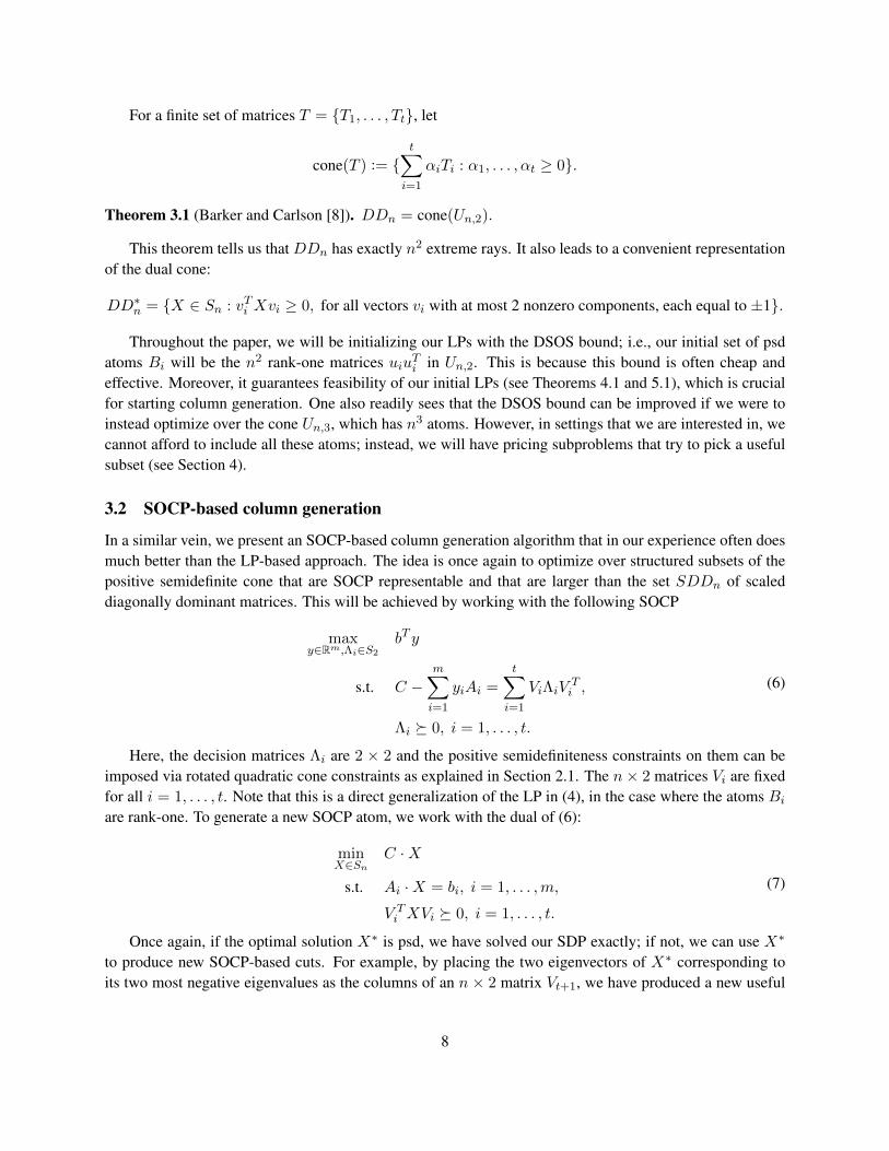
For a finite set of matrices T = {T1, . . . , Tt}, let
cone(T ) := {t∑i=1
αiTi : α1, . . . , αt ≥ 0}.
Theorem 3.1 (Barker and Carlson [8]). DDn = cone(Un,2).
This theorem tells us that DDn has exactly n2 extreme rays. It also leads to a convenient representationof the dual cone:
DD∗n = {X ∈ Sn : vTi Xvi ≥ 0, for all vectors vi with at most 2 nonzero components, each equal to ±1}.
Throughout the paper, we will be initializing our LPs with the DSOS bound; i.e., our initial set of psdatoms Bi will be the n2 rank-one matrices uiuTi in Un,2. This is because this bound is often cheap andeffective. Moreover, it guarantees feasibility of our initial LPs (see Theorems 4.1 and 5.1), which is crucialfor starting column generation. One also readily sees that the DSOS bound can be improved if we were toinstead optimize over the cone Un,3, which has n3 atoms. However, in settings that we are interested in, wecannot afford to include all these atoms; instead, we will have pricing subproblems that try to pick a usefulsubset (see Section 4).
3.2 SOCP-based column generation
In a similar vein, we present an SOCP-based column generation algorithm that in our experience often doesmuch better than the LP-based approach. The idea is once again to optimize over structured subsets of thepositive semidefinite cone that are SOCP representable and that are larger than the set SDDn of scaleddiagonally dominant matrices. This will be achieved by working with the following SOCP
maxy∈Rm,Λi∈S2
bT y
s.t. C −m∑i=1
yiAi =
t∑i=1
ViΛiVTi ,
Λi � 0, i = 1, . . . , t.
(6)
Here, the decision matrices Λi are 2 × 2 and the positive semidefiniteness constraints on them can beimposed via rotated quadratic cone constraints as explained in Section 2.1. The n× 2 matrices Vi are fixedfor all i = 1, . . . , t. Note that this is a direct generalization of the LP in (4), in the case where the atoms Biare rank-one. To generate a new SOCP atom, we work with the dual of (6):
minX∈Sn
C ·X
s.t. Ai ·X = bi, i = 1, . . . ,m,
V Ti XVi � 0, i = 1, . . . , t.
(7)
Once again, if the optimal solution X∗ is psd, we have solved our SDP exactly; if not, we can use X∗
to produce new SOCP-based cuts. For example, by placing the two eigenvectors of X∗ corresponding toits two most negative eigenvalues as the columns of an n × 2 matrix Vt+1, we have produced a new useful
8
atom. (Of course, we can also choose to add more pairs of eigenvectors and add multiple atoms.) As in theLP case, by construction, our bound can only improve in every iteration.
We will always be initializing our SOCP iterations with the SDSOS bound. It is not hard to see that thiscorresponds to the case where we have
(n2
)initial n× 2 atoms Vi, which have zeros everywhere, except for
a 1 in the first column in position j and a 1 in the second column in position k 6= j. We denote the set of allsuch n× 2 matrices by Vn,2
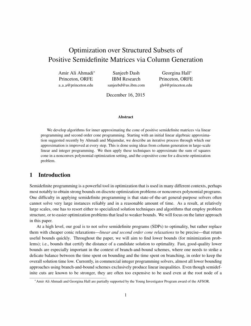
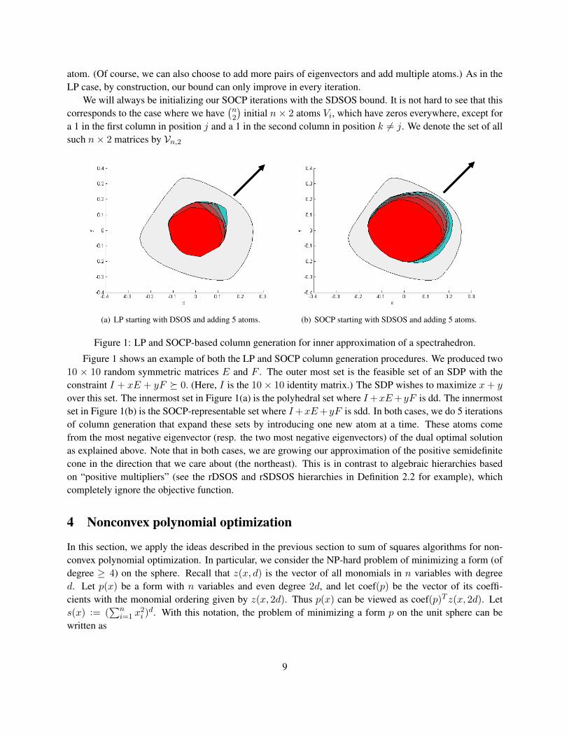
(a) LP starting with DSOS and adding 5 atoms. (b) SOCP starting with SDSOS and adding 5 atoms.
Figure 1: LP and SOCP-based column generation for inner approximation of a spectrahedron.
Figure 1 shows an example of both the LP and SOCP column generation procedures. We produced two10 × 10 random symmetric matrices E and F . The outer most set is the feasible set of an SDP with theconstraint I + xE + yF � 0. (Here, I is the 10× 10 identity matrix.) The SDP wishes to maximize x+ y
over this set. The innermost set in Figure 1(a) is the polyhedral set where I+xE+yF is dd. The innermostset in Figure 1(b) is the SOCP-representable set where I+xE+yF is sdd. In both cases, we do 5 iterationsof column generation that expand these sets by introducing one new atom at a time. These atoms comefrom the most negative eigenvector (resp. the two most negative eigenvectors) of the dual optimal solutionas explained above. Note that in both cases, we are growing our approximation of the positive semidefinitecone in the direction that we care about (the northeast). This is in contrast to algebraic hierarchies basedon “positive multipliers” (see the rDSOS and rSDSOS hierarchies in Definition 2.2 for example), whichcompletely ignore the objective function.
4 Nonconvex polynomial optimization
In this section, we apply the ideas described in the previous section to sum of squares algorithms for non-convex polynomial optimization. In particular, we consider the NP-hard problem of minimizing a form (ofdegree ≥ 4) on the sphere. Recall that z(x, d) is the vector of all monomials in n variables with degreed. Let p(x) be a form with n variables and even degree 2d, and let coef(p) be the vector of its coeffi-cients with the monomial ordering given by z(x, 2d). Thus p(x) can be viewed as coef(p)T z(x, 2d). Lets(x) := (
∑ni=1 x
2i )d. With this notation, the problem of minimizing a form p on the unit sphere can be
written as
9
maxλ
λ
s.t. p(x)− λs(x) ≥ 0, ∀x ∈ Rn. (8)
With the SOS programming approach, the following SDP is solved to get the largest scalar λ and an SOScertificate proving that p(x)− λs(x) is nonnegative:
maxλ,Y
λ
s.t. p(x)− λs(x) = zT (x, d)Y z(x, d) (9)
Y � 0.
The sum of squares certificate is directly read from an eigenvalue decomposition of the solution Y to theSDP above and has the form
p(x)− λs(x) ≥∑i
(zT (x, d)ui)2,
where Y =∑
i uiuTi . Since all sos polynomials are nonnegative, the optimal value of the SDP in (9) is a
lower bound to the optimal value of the optimization problem in (8). Unfortunately, before solving the SDP,we do not have access to the vectors ui in the decomposition of the optimal matrix Y . However, the factthat such vectors exist hints at how we should go about replacing Pn by a polyhedral restriction in (9): Ifthe constraint Y � 0 is changed to
Y =∑u∈U
αuuuT , αu ≥ 0, (10)
where U is a finite set, then (9) becomes an LP. This is one interpretation of Ahmadi and Majumdar’s workin [3, 4] where they replace Pn by DDn. Indeed, this is equivalent to taking U = Un,2 in (10), as shown inTheorem 3.1. We are interested in extending their results by replacing Pn by larger restrictions than DDn.A natural candidate for example would be obtained by changing Un,2 to Un,3. However, although Un,3 isfinite, it contains a very large set of vectors even for small values of n and d. For instance, when n = 30 andd = 4, Un,3 has over 66 million elements. Therefore we use column generation ideas to iteratively expandU in a manageable fashion. To initialize our procedure, we need to start with good enough atoms to have afeasible LP. The following result guarantees that replacing Y � 0 with Y ∈ DDn always yields an initialfeasible LP in the setting that we are interested in.
Theorem 4.1. For any form p of degree 2d, there exists λ ∈ R such that p(x)− λ(∑n
i=1 x2i )d is dsos.
Proof. As before, let s(x) = (∑n
i=1 x2i )d. We observe that the form s(x) is strictly in the interior of
DSOSn,2d. Indeed, by expanding out the expression we see that we can write s(x) as zT (x, d)Qz(x, d),where Q is a diagonal matrix with all diagonal entries positive. So Q is in the interior of DD(n+d−1
d ), and
hence s(x) is in the interior of DSOSn,2d. This entails that for α > 0 small enough, the form
(1− α)s(x) + αp(x)
will be dsos. Since DSOSn,2d is a cone, the form
(1− α)
αs(x) + p(x)
will also be dsos. By taking λ to be smaller than −1−αα , the claim is established.
10
As DDn ⊆ SDDn, the theorem above implies that replacing Y � 0 with Y ∈ SDDn also yields aninitial feasible SOCP. Motivated in part by this theorem, we will always start our LP-based iterative processwith the restriction that Y ∈ DDn. Let us now explain how we improve on this approximation via columngeneration.
Suppose we have a set U of vectors in Rn, whose outerproducts form all of the rank-one psd atoms thatwe want to consider. This set could be finite but very large, or even infinite. For our purposes U alwaysincludes Un,2, as we initialize our algorithm with the dsos relaxation. Let us consider first the case where Uis finite: U = {u1, . . . , ut}. Then the problem that we are interested in solving is
maxλ,αj
λ
s.t. p(x)− λs(x) = zT (x, d)Y z(x, d)
Y =t∑
j=1
αjujuTj , αj ≥ 0 for j = 1, . . . , t.
Suppose z(x, 2d) has m monomials and let the ith monomial in p(x) have coefficient bi, i.e., coef(p) =
(b1, . . . , bm)T . Also let si be the ith entry in coef(s(x)). We rewrite the previous problem as
maxλ,αj
λ
s.t. Ai · Y + λsi = bi for i = 1, . . . ,m
Y =
t∑j=1
αjujuTj , αj ≥ 0 for j = 1, . . . , t.
where Ai is a matrix that collects entries of Y that contribute to a coefficient corresponding to monomial iin z(x, 2d), when zT (x, d)Y z(x, d) is expanded out. The above is equivalent to
maxλ,αj
λ
s.t.∑j
αj(Ai · ujuTj ) + λsi = bi for i = 1, . . . ,m. (11)
αj ≥ 0 for j = 1, . . . , t.
The dual problem is
minµ
m∑i=1
µibi
s.t. (
m∑i=1
µiAi) · ujuTj ≥ 0, j = 1, . . . , t
m∑i=1
µisi = 1.
In the column generation framework, suppose we consider only a subset of the primal LP variables cor-responding to the matrices u1u
T1 , . . . , uku
Tk for some k < t (call this the reduced primal problem). Let
11
(α1, . . . , αk) stand for an optimal solution of the reduced primal problem and let µ = (µ1, . . . , µm) standfor an optimal dual solution. If we have
(
m∑i=1
µiAi) · ujuTj ≥ 0 for j = k + 1, . . . , t, (12)
then µ is an optimal dual solution for the original larger primal problem with columns 1, . . . , t. In otherwords, if we simply set αk+1 = · · · = αt = 0, then the solution of the reduced primal problem becomes asolution of the original primal problem. On the other hand, if (12) is not true, then suppose the condition isviolated for some uluTl . We can augment the reduced primal problem by adding the variable αl, and repeatthis process.
Let B =∑m
i=1 µiAi. We can test if (12) is false by solving the pricing subproblem:
minu∈U
uTBu. (13)
If uTBu < 0, then there is an element u in U such that the matrix uuT violates the dual constraint writtenin (12). Problem (13) may or may not be easy to solve depending on the set U . For example, an ambitiouscolumn generation strategy to improve on dsos (i.e., U = Un,2), would be to take U = Un,n; i.e., the set allvectors in Rn consisting of zeros, ones, and minus ones. In this case, the pricing problem (13) becomes
minu∈{0,±1}n
uTBu.
Unfortunately, the above problem generalizes the quadratic unconstrained boolean optimization problem(QUBO) and is NP-hard. Nevertheless, there are good heuristics for this problem (see e.g., [11],[16]) thatcan be used to find near optimal solutions very fast. While we did not pursue this pricing subproblem, we didconsider optimizing over Un,3. We refer to the vectors in Un,3 as “triples” for obvious reasons and generallyrefer to the process of adding atoms drawn from Un,3 as optimizing over “triples”.
Even though one can theoretically solve (13) with U = Un,3 in polynomial time by simple enumerationof n3 elements, this is very impractical. Our simple implementation is a partial enumeration and is imple-mented as follows. We iterate through the triples (in a fixed order), and test to see whether the conditionuTBu ≥ 0 is violated by a given triple u, and collect such violating triples in a list. We terminate theiteration when we collect a fixed number of violating triples (say t1). We then sort the violating triples byincreasing values of uTBu (remember, these values are all negative for the violating triples) and select the t2most violated triples (or fewer if less than t2 are violated overall) and add them to our current set of atoms.In a subsequent iteration we start off enumerating triples right after the last triple enumerated in the currentiteration so that we do not repeatedly scan only the same subset of triples. Although our implementation issomewhat straightforward and can be obviously improved, we are able to demonstrate that optimizing overtriples improves over the best bounds obtained by Ahmadi and Majumdar in a similar amount of time (seeSection 4.2).
We can also have pricing subproblems where the set U is infinite. Consider e.g. the case U = Rn in(13). In this case, if there is a feasible solution with a negative objective value, then the problem is clearlyunbounded below. Hence, we look for a solution with the smallest value of “violation” of the dual constraintdivided by the norm of the violating matrix. In other words, we want the expression uTBu/norm(uuT ) tobe as small as possible, where norm is the Euclidean norm of the vector consisting of all entries of uuT . Thisis the same as minimizing uTBu/||u||2. The eigenvector corresponding to the smallest eigenvalue yields
12
such a minimizing solution. This is the motivation behind the strategy described in the previous sectionfor our LP column generation scheme. In this case, we can use a similar strategy for our SOCP columngeneration scheme. We replace Y � 0 by Y ∈ SDDn in (9) and iteratively expand SDDn by using the“two most negative eigenvector technique” described in Section 3.2.
4.1 Experiments with a 10-variable quartic
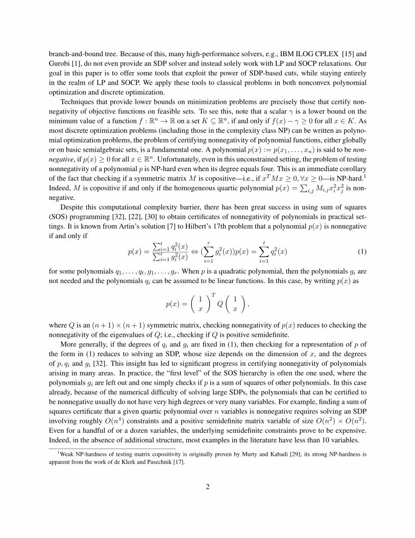
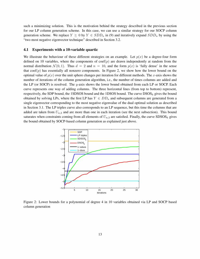
We illustrate the behaviour of these different strategies on an example. Let p(x) be a degree-four formdefined on 10 variables, where the components of coef(p) are drawn independently at random from thenormal distribution N (0, 1). Thus d = 2 and n = 10, and the form p(x) is ‘fully dense’ in the sensethat coef(p) has essentially all nonzero components. In Figure 2, we show how the lower bound on theoptimal value of p(x) over the unit sphere changes per iteration for different methods. The x-axis shows thenumber of iterations of the column generation algorithm, i.e., the number of times columns are added andthe LP (or SOCP) is resolved. The y-axis shows the lower bound obtained from each LP or SOCP. Eachcurve represents one way of adding columns. The three horizontal lines (from top to bottom) represent,respectively, the SDP bound, the 1SDSOS bound and the 1DSOS bound. The curve DSOSk gives the boundobtained by solving LPs, where the first LP has Y ∈ DDn and subsequent columns are generated from asingle eigenvector corresponding to the most negative eigenvalue of the dual optimal solution as describedin Section 3.1. The LP triples curve also corresponds to an LP sequence, but this time the columns that areadded are taken from Un,3 and are more than one in each iteration (see the next subsection). This boundsaturates when constraints coming from all elements of Un,3 are satisfied. Finally, the curve SDSOSk givesthe bound obtained by SOCP-based column generation as explained just above.
5 10 15 20 25 30−5.5
−5
−4.5
−4
−3.5
−3
−2.5
−2
−1.5
−1
iterations
SDPLP triplesSDSOSk
DSOSk
1−sdsos1−dsos
Figure 2: Lower bounds for a polynomial of degree 4 in 10 variables obtained via LP and SOCP basedcolumn generation
13
4.2 Larger computational experiments
In this section, we consider larger problem instances ranging from 15 variables to 40 variables, and we onlyapply our “triples” column generation strategy. Our problem instances are again fully dense and generatedin exactly the same way as the n = 10 example of the previous subsection.
To solve the triples pricing subproblem with our partial enumeration strategy, we set t1 to 300,000 andt2 to 5000. Thus in each iteration, we find up to 300,000 violated triples, and add up to 5000 of them. Inother words, we augment our LP by up to 5000 columns in each iteration. This is somewhat unusual as inpractice at most a few dozen columns are added in each iteration. The logic for this is that primal simplexis very fast in reoptimizing an LP when a small number of additional columns are added to an LP whoseoptimal basis is known. However, in our context, we observed that the associated LPs are very hard forthe simplex routines inside our LP solver (CPLEX 12.4) and take much more time than CPLEX’s interiorpoint solver. We therefore use CPLEX’s interior point (“barrier”) solver not only for the initial LP but forsubsequent LPs after adding columns. Because interior point solvers do not benefit significantly from warmstarts, each LP takes a similar amount of time to solve as the initial LP, and therefore it makes sense to add alarge number of columns in each iteration to amortize the time for each expensive solve over many columns.
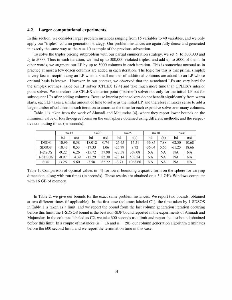
Table 1 is taken from the work of Ahmadi and Majumdar [4], where they report lower bounds on theminimum value of fourth-degree forms on the unit sphere obtained using different methods, and the respec-tive computing times (in seconds).
n=15 n=20 n=25 n=30 n=40bd t(s) bd t(s) bd t(s) bd t(s) bd t(s)
DSOS -10.96 0.38 -18.012 0.74 -26.45 15.51 -36.85 7.88 -62.30 10.68SDSOS -10.43 0.53 -17.33 1.06 -25.79 8.72 -36.04 5.65 -61.25 18.661-DSOS -9.22 6.26 -15.72 37.98 -23.58 369.08 NA NA NA NA
1-SDSOS -8.97 14.39 -15.29 82.30 -23.14 538.54 NA NA NA NASOS -3.26 5.60 -3.58 82.22 -3.71 1068.66 NA NA NA NA
Table 1: Comparison of optimal values in [4] for lower bounding a quartic form on the sphere for varyingdimension, along with run times (in seconds). These results are obtained on a 3.4 GHz Windows computerwith 16 GB of memory.
In Table 2, we give our bounds for the exact same problem instances. We report two bounds, obtainedat two different times (if applicable). In the first case (columns labeled C1), the time taken by 1-SDSOSin Table 1 is taken as a limit, and we report the bound from the last column generation iteration occuringbefore this limit; the 1-SDSOS bound is the best non-SDP bound reported in the experiments of Ahmadi andMajumdar. In the columns labeled as C2, we take 600 seconds as a limit and report the last bound obtainedbefore this limit. In a couple of instances (n = 15 and n = 20), our column generation algorithm terminatesbefore the 600 second limit, and we report the termination time in this case.
14
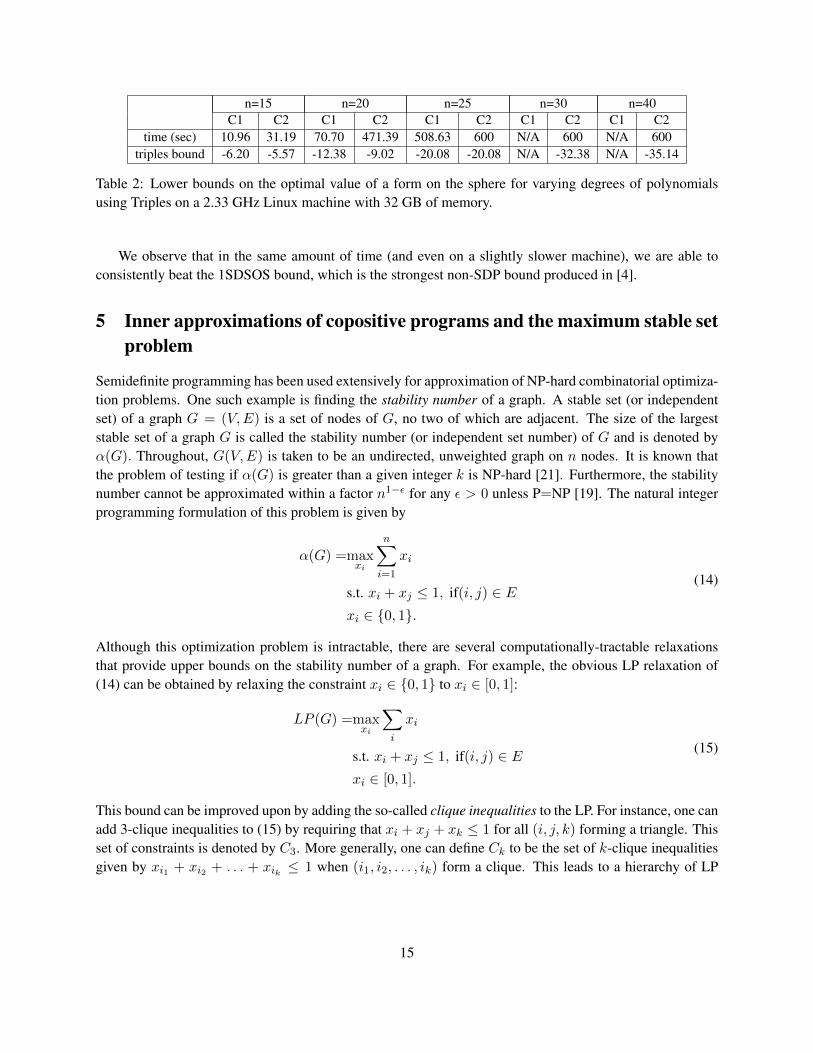
n=15 n=20 n=25 n=30 n=40C1 C2 C1 C2 C1 C2 C1 C2 C1 C2
time (sec) 10.96 31.19 70.70 471.39 508.63 600 N/A 600 N/A 600triples bound -6.20 -5.57 -12.38 -9.02 -20.08 -20.08 N/A -32.38 N/A -35.14
Table 2: Lower bounds on the optimal value of a form on the sphere for varying degrees of polynomialsusing Triples on a 2.33 GHz Linux machine with 32 GB of memory.
We observe that in the same amount of time (and even on a slightly slower machine), we are able toconsistently beat the 1SDSOS bound, which is the strongest non-SDP bound produced in [4].
5 Inner approximations of copositive programs and the maximum stable setproblem
Semidefinite programming has been used extensively for approximation of NP-hard combinatorial optimiza-tion problems. One such example is finding the stability number of a graph. A stable set (or independentset) of a graph G = (V,E) is a set of nodes of G, no two of which are adjacent. The size of the largeststable set of a graph G is called the stability number (or independent set number) of G and is denoted byα(G). Throughout, G(V,E) is taken to be an undirected, unweighted graph on n nodes. It is known thatthe problem of testing if α(G) is greater than a given integer k is NP-hard [21]. Furthermore, the stabilitynumber cannot be approximated within a factor n1−ε for any ε > 0 unless P=NP [19]. The natural integerprogramming formulation of this problem is given by
α(G) =maxxi
n∑i=1
xi
s.t. xi + xj ≤ 1, if(i, j) ∈ Exi ∈ {0, 1}.
(14)
Although this optimization problem is intractable, there are several computationally-tractable relaxationsthat provide upper bounds on the stability number of a graph. For example, the obvious LP relaxation of(14) can be obtained by relaxing the constraint xi ∈ {0, 1} to xi ∈ [0, 1]:
LP (G) =maxxi
∑i
xi
s.t. xi + xj ≤ 1, if(i, j) ∈ Exi ∈ [0, 1].
(15)
This bound can be improved upon by adding the so-called clique inequalities to the LP. For instance, one canadd 3-clique inequalities to (15) by requiring that xi + xj + xk ≤ 1 for all (i, j, k) forming a triangle. Thisset of constraints is denoted by C3. More generally, one can define Ck to be the set of k-clique inequalitiesgiven by xi1 + xi2 + . . . + xik ≤ 1 when (i1, i2, . . . , ik) form a clique. This leads to a hierarchy of LP
15
relaxations:LPk(G) = max
∑i
xi
xi ∈ [0, 1]
C2, . . . , Ck are satisfied.
(16)
Notice that for k = 2, this simply corresponds to (15), in other words, LP2(G) = LP (G).There are also semidefinite programming (SDP) relaxations that provide upper bounds to the stability
number. The most famous one perhaps is the Lovasz theta number ϑ(G) [25], which is defined as theoptimal value of the following SDP:
ϑ(G) :=maxXJ ·X
s.t. I ·X = 1,
Xi,j = 0, ∀(i, j) ∈ EX ∈ Pn.
(17)
Here J is the all-ones matrix and I is the identity matrix of size n. The Lovasz theta number is known toalways give at least as good of an upper bound as the LP in (15), even with the addition of clique inequalitiesof all sizes (there are exponentially many); see, e.g., [23, Section 6.5.2] for a proof. In other words,
ϑ(G) ≤ LPk(G),∀k.
An alternative SDP relaxation for stable set is due to de Klerk and Pasechnik. In [17], they show that thestability number can be obtained through a conic linear program over the set of copositive matrices. Namely,
α(G) = minλλ
s.t. λ(I +A)− J ∈ Cn,(18)
where A is the adjacency matrix of G. Replacing Cn by the restriction Pn + Nn, we obtain the aforemen-tioned relaxation through the following SDP
SDP (G) := minλ,X
λ
s.t. λ(I +A)− J ≥ XX ∈ Pn.
(19)
This latter SDP is more expensive to solve than the Lovasz SDP (17), but the bound that it obtains is alwaysat least as good (and sometimes strictly better). A proof of this statement is given in [17, Lemma 5.2], whereit is shown that (19) is an equivalent formulation of an SDP of Schrijver [36], which produces stronger upperbounds than (17).
Another reason for the interest in the copositive approach is that it allows for well-known SDP andLP hierarchies—developed respectively by Parrilo [31, Section 5] and de Klerk and Pasechnik [17]—thatproduce a sequence of improving bounds on the stability number. In fact, by appealing to Positivstellensatzresults of Polya [33], and Powers and Reznick [34], de Klerk and Pasechnik show that their LP hierarchyproduces the exact stability number in α2(G) number of steps [17, Theorem 4.1]. This immediately implies
16
the same result for stronger hierarchies, such as the SDP hierarchy of Parrilo [31], or the rDSOS and rSDSOShierarchies of Ahmadi and Majumdar [4].
One notable difficulty with the use of copositivity-based SDP relaxations such as (19) in applications isscalibility. For example, it takes more than 5 hours to solve (19) when the input is a randomly generatedErdos-Renyi graph with 300 nodes and edge probability p = 0.8. 3 Hence, instead of using (19), we willsolve a sequence of LPs/SOCPs generated in an iterative fashion. These easier optimization problems willprovide upper bounds on the stability number in a more reasonable amount of time, though they will beweaker than the ones obtained via (19).
We will derive both our LP and SOCP sequences from formulation (18) of the stability number. Toobtain the first LP in the sequence, we replace Cn by DDn + Nn (instead of replacing Cn by Pn + Nn aswas done in (19)) and get
DSOS1(G) := minλ,X
λ
s.t. λ(I +A)− J ≥ XX ∈ DDn.
(20)
This is an LP whose optimal value is a valid upperbound on the stability number as DDn ⊆ Pn.
Theorem 5.1. The LP in (20) is always feasible.
Proof. We need to show that for any n × n adjacency matrix A, there exists a diagonally dominant matrixD, a nonnegative matrix N , and a scalar λ such that
λ(I +A)− J = D +N. (21)
Notice first that λ(I + A)− J is a matrix with λ− 1 on the diagonal and at entry (i, j), if (i, j) is an edgein the graph, and with −1 at entry (i, j) if (i, j) is not an edge in the graph. If we denote by di the degree ofnode i, then let us take λ = n −mini di + 1 and D a matrix with diagonal entries λ − 1 and off-diagonalentries equal to 0 if there is an edge, and −1 if not. This matrix is diagonally dominant as there are at mostn − mini di minus ones on each row. Furthermore, if we take N to be a matrix with λ − 1 at the entries(i, j) where (i, j) is an edge in the graph, then (21) is satisfied and N ≥ 0.
Feasibility of this LP is important for us as it allows us to initiate column generation. By contrast, if wewere to replace the diagonal dominance constraint by a diagonal constraint for example, the LP could fail tobe feasible. This fact has been observed by de Klerk and Pasechnik in [17] and Bomze and de Klerk in [10].
To generate the next LP in the sequence via column generation, we think of the extreme-ray descriptionof the set of diagonally dominant matrices as explained in Section 3. Theorem 3.1 tells us that these aregiven by the matrices in Un,2 and so we can rewrite (20) as
DSOS1(G) := minλ,αi
λ
s.t. λ(I +A)− J ≥ X
X =∑
uiuTi ∈Un,2
αiuiuTi ,
αi ≥ 0, i = 1, . . . , n2.
(22)
3The solver in this case is MOSEK [2] and the machine used has 3.4GHz speed and 16GB RAM; see Table 4 for more results.The solution time with the popular SDP solver SeDuMi [37] e.g. would be several times larger.
17
The column generation procedure aims to add new matrix atoms to the existing set Un,2 in such a waythat the current bound DSOS1 improves. There are numerous ways of choosing these atoms. We focus firston the cutting plane approach based on eigenvectors. The dual of (22) is the LP
DSOS1(G) := maxX
J ·X
s.t. (A+ I) ·X = 1
X ≥ 0
(uiuTi ) ·X ≥ 0,∀uiuTi ∈ Un,2.
(23)
If our optimal solution X∗ to (23) is positive semidefinite, then we are obtaining the best bound we canpossibly produce, which is the SDP bound of (19). If this is not the case however, we pick our atom matrixto be the outer product uuT of the eigenvector u corresponding to the most negative eigenvalue of X∗. Theoptimal value of the LP
DSOS2(G) := maxX
J ·X
s.t. (A+ I) ·X = 1
X ≥ 0
(uiuTi ) ·X ≥ 0, ∀uiuTi ∈ Un,2
(uuT ) ·X ≥ 0
(24)
that we derive is guaranteed to be no worse than DSOS1 as the feasible set of (24) is smaller than thefeasible set of (23). Under mild nondegeneracy assumptions (satisfied, e.g., by uniqueness of the optimalsolution to (23)), the new bound will be strictly better. By reiterating the same process, we create a sequenceof LPs whose optimal values DSOS1, DSOS2, . . . are a nonincreasing sequence of upper bounds on thestability number.
Generating the sequence of SOCPs is done in an analogous way. Instead of replacing the constraintX ∈ Pn in (19) by X ∈ DDn, we replace it by X ∈ SDDn and get
SDSOS1(G) := minλ,X
λ
s.t. λ(I +A)− J ≥ XX ∈ SDDn.
(25)
Once again, we need to reformulate the problem in such a way that the set of scaled diagonally dominantmatrices is described as some combination of psd “atom” matrices. In this case, we can write any matrixX ∈ SDDn as
X =∑
Vi∈Vn,2
Vi
(a1i a2
i
a2i a3
i
)V Ti ,
where a1i , a
2i , a
3i are variables making the 2×2 matrix psd, and the Vi’s are our atoms. Recall from Section 3
that the set Vn,2 consists of all n×2 matrices which have zeros everywhere, except for a 1 in the first columnin position j and a 1 in the second column in position k 6= j. This gives rise to an equivalent formulation of
18
(25):SDSOS1(G) := min
λ,aji
λ
s.t. λ(I +A)− J ≥ X
X =∑
Vi∈Vn,2
Vi
(a1i a2
i
a2i a3
i
)V Ti(
a1i a2
i
a2i a3
i
)� 0, i = 1, . . . ,
(n
2
).
(26)
Just like the LP case, we now want to generate one (or more) n× 2 matrix V to add to the set {Vi}i so thatthe bound SDSOS1 improves. We do this again by using a cutting plane approach originating from the dualof (26):
SDSOS1(G) := maxX
J ·X
s.t. (A+ I) ·X = 1
X ≥ 0
V Ti ·XVi � 0, i = 1, . . . ,
(n
2
).
(27)
Note that strong duality holds between this primal-dual pair as it is easy to check that both problems arestrictly feasible. We then take our new atom to be
V = (w1 w2),
where w1 and w2 are two eigenvectors corresponding to the two most negative eigenvalues of X∗, theoptimal solution of (27). If X∗ only has one negative eigenvalue, we add a linear constraint to our problem;if X∗ � 0, then the bound obtained is identical to the one obtained through SDP (19) and we cannot hopeto improve. Our next iterate is therefore
SDSOS2(G) := maxX
J ·X
s.t. (A+ I) ·X = 1
X ≥ 0
V Ti ·XVi � 0, i = 1, . . . ,
(n
2
)V T ·XV � 0.
(28)
Note that the optimization problems generated iteratively in this fashion always remain SOCPs and theiroptimal values form a nonincreasing sequence of upper bounds on the stability number.
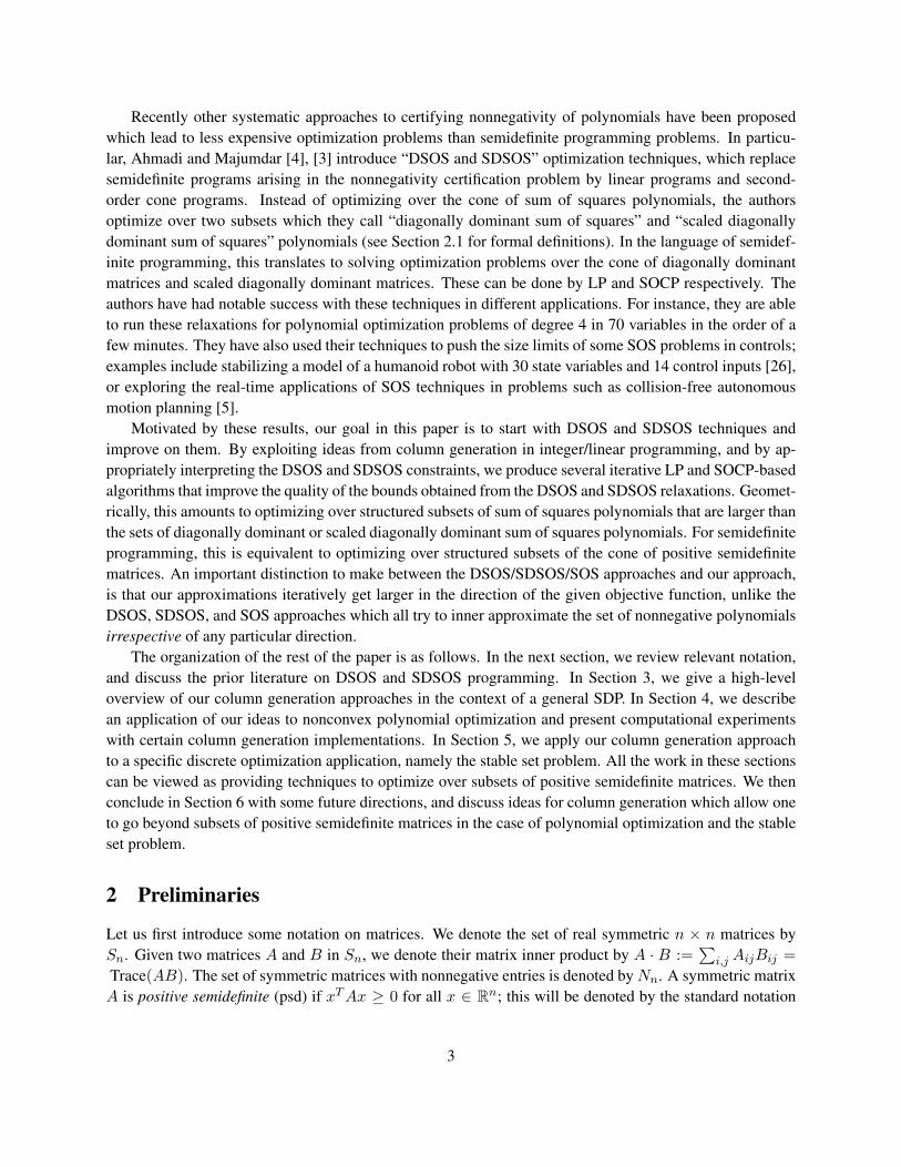
To illustrate the column generation method for both LPs and SOCPs, we consider the complement ofthe Petersen graph as shown in Figure 3(a) as an example. The stability number of this graph is 2 and one ofits maximum stable sets is designated by the two white nodes. In Figure 3(b), we compare the upper boundobtained via (19) and the bounds obtained using the iterative LPs and SOCPs as described in (24) and (28).
Note that it takes 3 iterations for the SOCP sequence to produce an upperbound strictly within oneunit of the actual stable set number (which would immediately tell us the value of α), whereas it takes 13iterations for the LP sequence to do the same. It is also interesting to compare the sequence of LPs/SOCPs
19
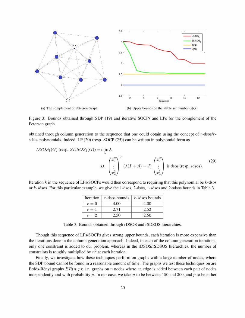
(a) The complement of Petersen Graph
2 4 6 8 10 121.5
2
2.5
3
3.5
4
4.5
iterations
DSOSk
SDSOSk
SDP
α(G)
(b) Upper bounds on the stable set number α(G)
Figure 3: Bounds obtained through SDP (19) and iterative SOCPs and LPs for the complement of thePetersen graph.
obtained through column generation to the sequence that one could obtain using the concept of r-dsos/r-sdsos polynomials. Indeed, LP (20) (resp. SOCP (25)) can be written in polynomial form as
DSOS1(G) (resp. SDSOS1(G)) = minλλ
s.t.
x21...x2n
T
(λ(I +A)− J)
x21...x2n
is dsos (resp. sdsos).(29)
Iteration k in the sequence of LPs/SOCPs would then correspond to requiring that this polynomial be k-dsosor k-sdsos. For this particular example, we give the 1-dsos, 2-dsos, 1-sdsos and 2-sdsos bounds in Table 3.
Iteration r-dsos bounds r-sdsos boundsr = 0 4.00 4.00r = 1 2.71 2.52r = 2 2.50 2.50
Table 3: Bounds obtained through rDSOS and rSDSOS hierarchies.
Though this sequence of LPs/SOCPs gives strong upper bounds, each iteration is more expensive thanthe iterations done in the column generation approach. Indeed, in each of the column generation iterations,only one constraint is added to our problem, whereas in the rDSOS/rSDSOS hierarchies, the number ofconstraints is roughly multiplied by n2 at each iteration.
Finally, we investigate how these techniques perform on graphs with a large number of nodes, wherethe SDP bound cannot be found in a reasonable amount of time. The graphs we test these techniques on areErdos-Renyi graphs ER(n, p); i.e. graphs on n nodes where an edge is added between each pair of nodesindependently and with probability p. In our case, we take n to be between 150 and 300, and p to be either
20
0.3 or 0.8 so as to experiment with both medium and high density graphs.4
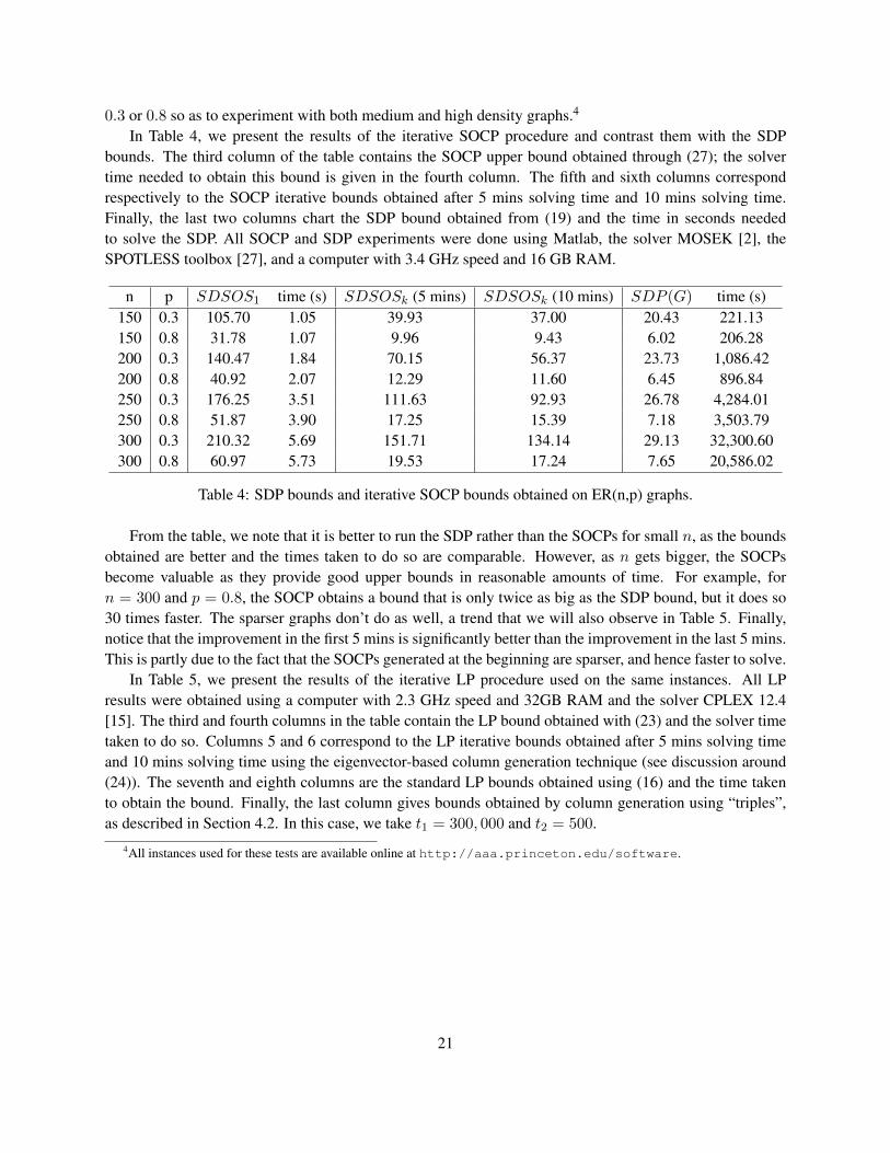
In Table 4, we present the results of the iterative SOCP procedure and contrast them with the SDPbounds. The third column of the table contains the SOCP upper bound obtained through (27); the solvertime needed to obtain this bound is given in the fourth column. The fifth and sixth columns correspondrespectively to the SOCP iterative bounds obtained after 5 mins solving time and 10 mins solving time.Finally, the last two columns chart the SDP bound obtained from (19) and the time in seconds neededto solve the SDP. All SOCP and SDP experiments were done using Matlab, the solver MOSEK [2], theSPOTLESS toolbox [27], and a computer with 3.4 GHz speed and 16 GB RAM.
n p SDSOS1 time (s) SDSOSk (5 mins) SDSOSk (10 mins) SDP (G) time (s)150 0.3 105.70 1.05 39.93 37.00 20.43 221.13150 0.8 31.78 1.07 9.96 9.43 6.02 206.28200 0.3 140.47 1.84 70.15 56.37 23.73 1,086.42200 0.8 40.92 2.07 12.29 11.60 6.45 896.84250 0.3 176.25 3.51 111.63 92.93 26.78 4,284.01250 0.8 51.87 3.90 17.25 15.39 7.18 3,503.79300 0.3 210.32 5.69 151.71 134.14 29.13 32,300.60300 0.8 60.97 5.73 19.53 17.24 7.65 20,586.02
Table 4: SDP bounds and iterative SOCP bounds obtained on ER(n,p) graphs.
From the table, we note that it is better to run the SDP rather than the SOCPs for small n, as the boundsobtained are better and the times taken to do so are comparable. However, as n gets bigger, the SOCPsbecome valuable as they provide good upper bounds in reasonable amounts of time. For example, forn = 300 and p = 0.8, the SOCP obtains a bound that is only twice as big as the SDP bound, but it does so30 times faster. The sparser graphs don’t do as well, a trend that we will also observe in Table 5. Finally,notice that the improvement in the first 5 mins is significantly better than the improvement in the last 5 mins.This is partly due to the fact that the SOCPs generated at the beginning are sparser, and hence faster to solve.
In Table 5, we present the results of the iterative LP procedure used on the same instances. All LPresults were obtained using a computer with 2.3 GHz speed and 32GB RAM and the solver CPLEX 12.4[15]. The third and fourth columns in the table contain the LP bound obtained with (23) and the solver timetaken to do so. Columns 5 and 6 correspond to the LP iterative bounds obtained after 5 mins solving timeand 10 mins solving time using the eigenvector-based column generation technique (see discussion around(24)). The seventh and eighth columns are the standard LP bounds obtained using (16) and the time takento obtain the bound. Finally, the last column gives bounds obtained by column generation using “triples”,as described in Section 4.2. In this case, we take t1 = 300, 000 and t2 = 500.
4All instances used for these tests are available online at http://aaa.princeton.edu/software.
21
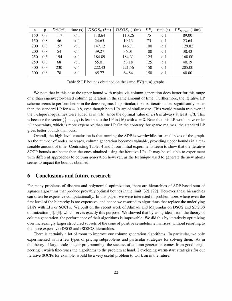
n p DSOS1 time (s) DSOSk (5m) DSOSk (10m) LP2 time (s) LPtriples (10m)150 0.3 117 < 1 110.64 110.26 75 < 1 89.00150 0.8 46 < 1 24.65 19.13 75 < 1 23.64200 0.3 157 < 1 147.12 146.71 100 < 1 129.82200 0.8 54 < 1 39.27 36.01 100 < 1 30.43250 0.3 194 < 1 184.89 184.31 125 < 1 168.00250 0.8 68 < 1 55.01 53.18 125 < 1 40.19300 0.3 230 < 1 222.43 221.56 150 < 1 205.00300 0.8 78 < 1 65.77 64.84 150 < 1 60.00
Table 5: LP bounds obtained on the same ER(n, p) graphs.
We note that in this case the upper bound with triples via column generation does better for this rangeof n than eigenvector-based column generation in the same amount of time. Furthermore, the iterative LPscheme seems to perform better in the dense regime. In particular, the first iteration does significantly betterthan the standard LP for p = 0.8, even though both LPs are of similar size. This would remain true even ifthe 3-clique inequalities were added as in (16), since the optimal value of LP3 is always at least n/3. Thisis because the vector (1
3 , . . . ,13) is feasible to the LP in (16) with k = 3. Note that this LP would have order
n3 constraints, which is more expensive than our LP. On the contrary, for sparse regimes, the standard LPgives better bounds than ours.
Overall, the high-level conclusion is that running the SDP is worthwhile for small sizes of the graph.As the number of nodes increases, column generation becomes valuable, providing upper bounds in a rea-sonable amount of time. Contrasting Tables 4 and 5, our initial experiments seem to show that the iterativeSOCP bounds are better than the ones obtained using the iterative LPs. It may be valuable to experimentwith different approaches to column generation however, as the technique used to generate the new atomsseems to impact the bounds obtained.
6 Conclusions and future research
For many problems of discrete and polynomial optimization, there are hierarchies of SDP-based sum ofsquares algorithms that produce provably optimal bounds in the limit [32], [22]. However, these hierarchiescan often be expensive computationally. In this paper, we were interested in problem sizes where even thefirst level of the hierarchy is too expensive, and hence we resorted to algorithms that replace the underlyingSDPs with LPs or SOCPs. We built on the recent work of Ahmadi and Majumdar on DSOS and SDSOSoptimization [4], [3], which serves exactly this purpose. We showed that by using ideas from the theory ofcolumn generation, the performance of their algorithms is improvable. We did this by iteratively optimizingover increasingly larger structured subsets of the cone of positive semidefinite matrices, without resorting tothe more expensive rDSOS and rSDSOS hierarchies.
There is certainly a lot of room to improve our column generation algorithms. In particular, we onlyexperimented with a few types of pricing subproblems and particular strategies for solving them. As inthe theory of large-scale integer programming, the success of column generation comes from good “engi-neering”, which fine-tunes the algorithms to the problem at hand. Developing warm-start strategies for ouriterative SOCPs for example, would be a very useful problem to work on in the future.
22
Here is another interesting research direction, which for illustrative purposes we outline for the problemstudied in Section 4; i.e., minimizing a form on the sphere. Recall that given a form p of degree 2d, we aretrying to find the largest λ such that p(x)− λ(
∑ni=1 x
2i )d is a sum of squares. Instead of solving this sum of
squares program, we looked for the largest λ for which we could write p(x)− λ as a conic combination ofa certain set of nonnegative polynomials. These polynomials for us were always either a single square or asum of squares of polynomials. There are polynomials, however, that are nonnegative but not representableas a sum of squares. Two classic examples [28], [14] are the Motzkin polynomial
M(x, y, z) = x6 + y4z2 + y2z4 − 3x2y2z2,
and the Choi-Lam polynomial
CL(w, x, y, z) = w4 + x2y2 + y2z2 + x2z2 − 4wxyz.
Either of these polynomials can be shown to be nonnegative using the arithmetic mean-geometric mean(am-gm) inequality, which states that if x1, . . . , xk ∈ R, then
x1, . . . , xk ≥ 0⇒ (k∑i=1
xi)/k ≥ (Πki=1xi)
1k .
For example, in the case of the Motzkin polynomial, it is clear that the monomials x6, y4z2 and y2z4 arenonnegative for all x, y, z ∈ R, and letting x1, x2, x3 stand for these monomials respectively, the am-gminequality implies that
x6 + y4z2 + y2z4 ≥ 3x2y2z2 for all x, y, z ∈ R.
These polynomials are known to be extreme in the cone of nonnegative polynomials and they cannot bewritten as a sum of squares (sos) [35].
It would be interesting to study the separation problems associated with using such non-sos polynomialsin column generation. We briefly present one separation algorithm for a family of polynomials whose non-negativity is provable through the am-gm inequality and includes the Motzkin and Choi-Lam polynomials.This will be a relatively easy-to-solve integer program in itself, whose goal is to find a polynomial q amongstthis family which is to be added as our new “nonnegative atom”.
The family of n-variate polynomials under consideration consists of polynomials with only k+1 nonzerocoefficients, with k of them equal to one, and one equal to −k. (Notice that the Motzkin and the Choi-Lampolynomials are of this form with k equal to three and four respectively.) Letm be the number of monomialsin p. Given a dual vector µ of (11) of dimension m, one can check if there exists a nonnegative degree 2d
polynomial q(x) in our family such that µ · coef(q(x)) < 0. This can be done by solving the following
23
integer program (we assume that p(x) =∑m
i=1 xαi):
minc,y
m∑i=1
µici −m∑i=1
kµiyi (30)
s.t.∑
i:αi is evenαici = k
m∑i=1
αiyi
m∑i=1
ci = k
m∑i=1
yi = 1
ci ∈ {0, 1}, yi ∈ {0, 1}, i = 1, . . . ,m, ci = 0 if αi is not even.
Here, we have αi ∈ Nn and the variables ci, yi form the coefficients of the polynomial q. The above integerprogram has 2m variables, but only n+ 2 constraints (not counting the integer constraints). If a polynomialq(x) with a negative objective value is found, then one can add it as a new atom for column generation.In our specific randomly generated polynomial optimization examples, such polynomials did not seem tohelp in our preliminary experiments. Nevertheless, it would be interesting to consider other instances andproblem structures.
Similarly, in the column generation approach to obtaining inner approximations of the copositive cone,one need not stick to positive demidefinite matrices. It is known that the 5 × 5 “Horn matrix” [13] forexample is extreme in the copositive cone but cannot be written as the sum of a nonnegative and a positivesemidefinite matrix. One could define a separation problem for a family of Horn-like matrices and add themin a column generation approach. Exploring such strategies is left for future research.
7 Acknowledgments
We are grateful to Anirudha Majumdar for insightful discussions and for his help with some of the numericalexperiments in this paper.
References
[1] Gurobi optimizer reference manual. URL: http://www. gurobi. com, 2012.
[2] MOSEK reference manual, 2013. Version 7. Latest version available at http://www.mosek.com/.
[3] A. A. Ahmadi and A. Majumdar. DSOS and SDSOS optimization: LP and SOCP-based alternatives tosum of squares optimization. In Proceedings of the 48th Annual Conference on Information Sciencesand Systems. Princeton University, 2014.
[4] A. A. Ahmadi and A. Majumdar. DSOS and SDSOS: more tractable alternatives to sum of squaresand semidefinite optimization. In preparation, 2015.
24
[5] A. A. Ahmadi and A. Majumdar. Some applications of polynomial optimization in operations researchand real-time decision making. Prepint available at http://arxiv.org/abs/1504.06002. Toappear in Optimization Letters, 2015.
[6] F. Alizadeh and D. Goldfarb. Second-order cone programming. Mathematical programming, 95(1):3–51, 2003.
[7] E. Artin. Uber die Zerlegung definiter Funktionen in Quadrate. In Abhandlungen aus dem mathema-tischen Seminar der Universitat Hamburg, volume 5, pages 100–115. Springer, 1927.
[8] G. Barker and D. Carlson. Cones of diagonally dominant matrices. Pacific Journal of Mathematics,57(1):15–32, 1975.
[9] C. Barnhart, E. L. Johnson, G. L. Nemhauser, M. W. Savelsbergh, and P. H. Vance. Branch-and-price:Column generation for solving huge integer programs. Operations research, 46(3):316–329, 1998.
[10] I. M. Bomze and E. de Klerk. Solving standard quadratic optimization problems via linear, semidefiniteand copositive programming. Journal of Global Optimization, 24(2):163–185, 2002.
[11] E. Boros, P. Hammer, and G. Tavares. Local search heuristics for quadratic unconstrained binaryoptimization (qubo). Journal of Heuristics, 13(2):99–132, 2007.
[12] S. Burer. Copositive programming. In Handbook on semidefinite, conic and polynomial optimization,pages 201–218. Springer, 2012.
[13] S. Burer, K. M. Anstreicher, and M. Dur. The difference between 5× 5 doubly nonnegative andcompletely positive matrices. Linear Algebra and its Applications, 431(9):1539–1552, 2009.
[14] M. D. Choi and T. Y. Lam. Extremal positive semidefinite forms. Math. Ann., 231:1–18, 1977.
[15] CPLEX. V12. 4: Users manual for CPLEX. International Business Machines Corporation,46(53):157.
[16] S. Dash. A note on QUBO instances defined on Chimera graphs. arXiv preprint arXiv:1306.1202,2013.
[17] E. de Klerk and D. Pasechnik. Approximation of the stability number of a graph via copositive pro-gramming. SIAM Journal on Optimization, 12(4):875–892, 2002.
[18] G. Desaulniers, J. Desrosiers, and M. M. Solomon. Column generation, volume 5. Springer Science& Business Media, 2006.
[19] J. Hastad. Clique is hard to approximate within n1−ε. In Proceedings of the 37th Annual Symposiumon Foundations of Computer Science.
[20] D. Hilbert. Uber die Darstellung Definiter Formen als Summe von Formenquadraten. Math. Ann., 32,1888.
[21] R. M. Karp. Reducibility among combinatorial problems. Springer, 1972.
25
[22] J. B. Lasserre. Global optimization with polynomials and the problem of moments. SIAM Journal onOptimization, 11(3):796–817, 2001.
[23] M. Laurent and F. Vallentin. Lecture Notes on Semidefinite Optimization. 2012.
[24] M. S. Lobo, L. Vandenberghe, S. Boyd, and H. Lebret. Applications of second-order cone program-ming. Linear algebra and its applications, 284(1):193–228, 1998.
[25] L. Lovasz. On the Shannon capacity of a graph. Information Theory, IEEE Transactions on, 25(1):1–7,1979.
[26] A. Majumdar, A. A. Ahmadi, and R. Tedrake. Control and verification of high-dimensional systemsvia DSOS and SDSOS optimization. In Proceedings of the 53rd IEEE Conference on Decision andControl, 2014.
[27] A. Megretski. SPOT: systems polynomial optimization tools. 2013.
[28] T. S. Motzkin. The arithmetic-geometric inequality. In Inequalities, pages 205–224. Academic Press,New York, 1967.
[29] K. G. Murty and S. N. Kabadi. Some NP-complete problems in quadratic and nonlinear programming.Mathematical Programming, 39:117–129, 1987.
[30] Y. Nesterov. Squared functional systems and optimization problems. In High performance optimiza-tion, volume 33 of Appl. Optim., pages 405–440. Kluwer Acad. Publ., Dordrecht, 2000.
[31] P. A. Parrilo. Structured semidefinite programs and semialgebraic geometry methods in robustness andoptimization. PhD thesis, California Institute of Technology, May 2000.
[32] P. A. Parrilo. Semidefinite programming relaxations for semialgebraic problems. Mathematical Pro-gramming, 96(2, Ser. B):293–320, 2003.
[33] G. Polya. Uber positive Darstellung von Polynomen. Vierteljschr. Naturforsch. Ges. Zurich, 73:141–145, 1928.
[34] V. Powers and B. Reznick. A new bound for Polya’s theorem with applications to polynomials positiveon polyhedra. Journal of Pure and Applied Algebra, 164(1):221–229, 2001.
[35] B. Reznick. Some concrete aspects of Hilbert’s 17th problem. In Contemporary Mathematics, volume253, pages 251–272. American Mathematical Society, 2000.
[36] A. Schrijver. A comparison of the Delsarte and Lovasz bounds. Information Theory, IEEE Transac-tions on, 25(4):425–429, 1979.
[37] J. Sturm. SeDuMi version 1.05, Oct. 2001. Latest version available athttp://sedumi.ie.lehigh.edu/.
26