Embed Size (px)
Citation preview

http://repository.osakafu-u.ac.jp/dspace/
Title Analysis of Cutting Temperature of Drill Point
Author(s)Ogawa, Koichi; Adachi, Katsushige; Sakurai, Keizo; Niba, Ralph; Takas
hima, Yoshinao
Editor(s)
CitationBulletin of University of Osaka Prefecture. Series A, Engineering and nat
ural sciences. 1991, 40(1), p.137-148
Issue Date 1991-10-30
URL http://hdl.handle.net/10466/8535
Rights

137
Analysis of Cutting Temperature of Drill Point
Koichi OGAwA,' Katsushige ADAcHI," Keizo SAKuRAI""
Ralph NIBA""and Yoshinao TAKAsHIMA"
(Received June 15, 1991)
The main objective of the present paper is to discuss cutting temperature ofthe drill point in low frequency vibratory drilling of stainless steel (SUS 304).
Although many studies dealing with drill wear in conventional drilling havebeen presented, there has been hitherto no study dealing with cutting tempera-
ture of the drill point in low frequency vibratory drilling of SUS 304.
For this reason, cutting temperature in low frequency vibratory drilling ofSUS 304 was selected as the subject of study, that is, cutting temperature inthe drill face was measured by utilizing cobalt high speed steel drills brazed
with sheathed thermocouples, and the experimental results were comparedwith those of conventional drilling. Futhermore, distribution of cutting tem-perature in the drill point was computed by the finite element method.
From this study, distribution of cutting temperature in the drill point was
clarified.
1. Introduction
A large proportion of metal machining processes is covered by the process of hole
making. As a result of this widespread use of drills, the automation of the drilling
process is being vigorously pursued.However, problems such as extended drill Iife,
efficient chip disposal, excellent hole finish and so on have to be realized to fully
meet automatlon requlrements.
Whereas the use of tough materials such as stainless steel, titanium alloys has
been gaining ground, the effective drilling of these tough materials is marred by lots
of limitations which have to be overcome. The drilling of these tough materials in
particular is one of the difficult problems being faced by the metal machining
industry. One of the problems confronted when drilling tough materials is poor chip
disposal, thus, giving rise to an increase in cutting edge temperature. This drawback
is attributed to the very low heat conductivity and the tendency for these materials
to easily work harden. Another striking problem associated with the drilling of
tough materials is the severe adherence of chips on the drill face thus, hampering the
drilling action.
*
**
Course of Instrument Science, College of Integrated Arts and Sciences.
Faculty of Engineering, Osaka Sangyo University
138 Koichi OGAWA, Katsushige ADACHI, Keizo SAKURAI Ralph NIBA and Yoshinao TAKASHIMA
Low frequency vibratory drilling is one of the drilling methods believed suited to
drilling tough materials. Surprisingly so far, there has been very little research on
this promising drilling method. The only prominent study on vibratory drilling in
tough materials was reported by E. A Satel.
Considering the strategic importance of stainless steel, hole making in stainless
steel (SUS 304) was taken up as the theme of study by the authors. Special attention
is paid to the drill point temperature which has a direct bearing on the performance
of a tool. In addition, cutting forces (thrust, torque) and tool wear are also given
consideration. The correlation between cutting temperature and tool wear is looked
into besides, the three dimensional heat conduction analysis of the cutting edge by
the finite element method is undertaken to study the temperature distribution at the
face and flank.
2. Experimental device and method
2. 1 Device
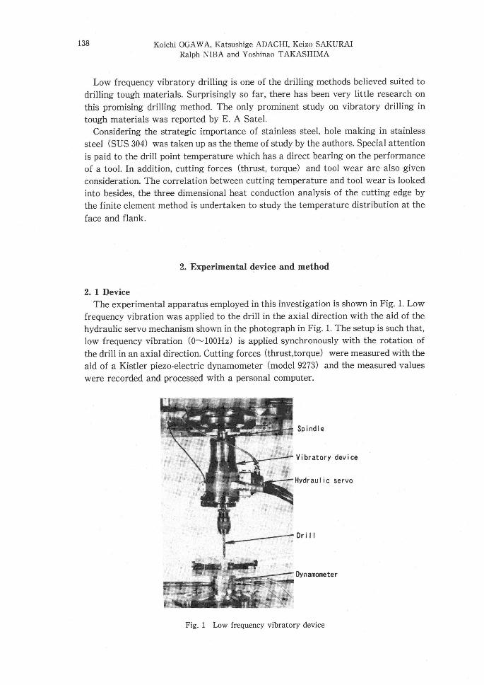
The experimental apparatus employed in this investigation is shown in Fig. 1. Low
frequency vibration was applied to the drill in the axial direction with the aid of the
hydraulic servo mechanism shown in the photograph in Fig. 1. The setup is such that,
low frequency vibration (O'--100Hz) is applied synchronously with the rotation of
the drill in an axial direction. Cutting forces (thrust,torque) were measured with the
aid of a Kistler piezo-electric dynamometer (model 9273) and the measured values
were recorded and processed with a personal computer.
ntee.
ts・, xt ・
ee
Spindle
Vibratory device
Hydraulic servo
Dril1
Dynatnometer
Fig. 1 Low frequency vibratory device
139
Analysis of C"tting 7timpemtu7e of Dnil Iloint
2. 2 Cutting temperature measurement A sheathed thermocouple was employed to measure the cutting edge temperature.
There are numerous research on cutting temperature but to the best of our knowl-
edge there is none on drill face temperature measurement.
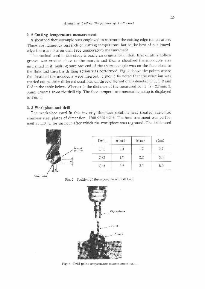
The method used in this study is really an originality in that, first of all, a hollow
groove was created close to the margin and then a sheathed thermocouple was
implanted in it, making sure one end of the thermocouple was on the face close to
the flute and then the drilling action was performed. Fig. 2 shows the points where
the sheathed thermocouple were inserted. It should be noted that the insertion was
carried out at three different positions, on three different drills denoted C'1, C-2 and
C-3 in the table below. Where r is the distance of the measured point (r=2.7mm, 3.
5mm, 5.9mm) from the drill tip. The face temperature measuring setup is displayed
in Fig. 3.
2. 3 Workpiece and drill
The workpiece used in this investigation was solution heat treated austenitic
stainless steel plates of dimension (200×300×20). The heat treatment was perfor-med at 1100eC for an hour after which the workpiece was reground. The drills used
Mesufedpesitien
Drill a(mm) b(mm) r(mn)
C-1 1.3 1.7 2.7
C-2 1.7 2.2 3.5
C-3 3.2 3.1 5.9
Chieel petnt
Fig. 2 Position of thermocouple on drill face
t/.ve
Wbrkpiecex
Chuck
Fig. 3 Drill point temperature measurement setup
140 Koichi OGAWA, Katsushige ADACHI, Keizo SAKURAI Ralph NIBA and Yoshinao TAKASHIMA
were cobalt high speed steel drills (JIS SKH56)of diameter 10mm. A model of the
drill with an inserted thermocouple is shown in Fig. 4. In order to minimize varia-
tions,only drills from the same lot were used. A water soluble lubricant (JSIS W2-3)
was employed and the rate of flow was held constant at 3.2 1/min.
gee
Fig. 4
geesseq,eewyinag,watrwewpagma/.ww.;-,:'"g
Photograph of drill with inserted thermocouple
3. Results and discussion
3. 1 Cutting forces and tool wear
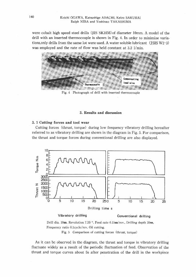
Cutting forces (thrust, torque) during low frequency vibratory drilling hereafter
referred to as vibratory drilling are shown in the diagram in Fig. 5. For comparison,
the thrust and torque forces during conventional drilling are also displayed.
Ezg9R
zu=L̀b
10
8
6
4
2
E)cx)8
2500
am15001OOO
am oO 5 10 15 20 250 5 10 15 mo Drilling time s
Vibratory drilting Conventional drilling
Drill dia. 10mm, Revolution 7.3S-', Feed rate O.15mn/rev., Drilling depth 20mm,
Frequency ratio O.lcycle/rev, Oil cutting.
Fig. 5 Comparison of cutting forces (thrust, torque)
as
As it can be observed in the diagram, the thrust and torque in vibratory drilling
fluctuate widely as a result of the periodic fluctuation of feed. Observation of the
thrust and torque curves about 5s after penetration of the drill in the workpiece

141
Analysis of Cutting 7;7mPerzzture of Dn'll Point
reveal in the case of vibratory drilling, a thrust force of about 1600N'v2050N, while
the torque force is about 5.0Nmev6.6Nm. The static component of these forces that
is the average of the periodic fluctuation, are thrust force of 1825N and torque force
of 5.8 Nm. Whereas, the conventional drilling thrust and torque curves yield readings
of 2000N and 6.3Nm respectively. A look at the curves in the diagram, reveal that
thrust and torque forces for vibratory drilling are 23% and 27% lower than those in
conventional drilling.
A look at the photographs of both drilling methods displayed in Fig. 6 reveal the
absence of built-up edge on the face and just little wear on the chisel, while wear of
the cutting edge of drills employed in the vibratory drilling tests is fairly uniform in
nature whereas, considerable wear can be noticed on the outer corners of drills
employed in conventional drilling tests. The wear of the cutting edges on the outer
corners proceeds remarkably fast during conventional drilling leading to the accu-
mulation of built-up edges on the chisel causing chips to pack easily in the hole
thereby hastening tool failure.
Imm -
Conventional VibratoryDrill dia. 10mm, Revolution 7.3 S2', Feed rate O.15mm!rev., Drilling depth 20mm,
Frequency ratio O.lcyclelrev., Oil cutting
Fig. 6 Comparison of tool wear
From the viewpoint of tool wear and cutting forces, the above results reveal the
superiority of vibratory drilling over conventional drilling. The main reasons for this
superiority are the reduction in friction heat between the workpiece and tool as well
as the curb in built-up edge formation during vibratory drilling. Wear of the cutting
edges is believed to be influenced especially by friction heat.
3. 2 Cutting edge temperature
In the foregoing test, face temperature mesurement for both drilling methods were
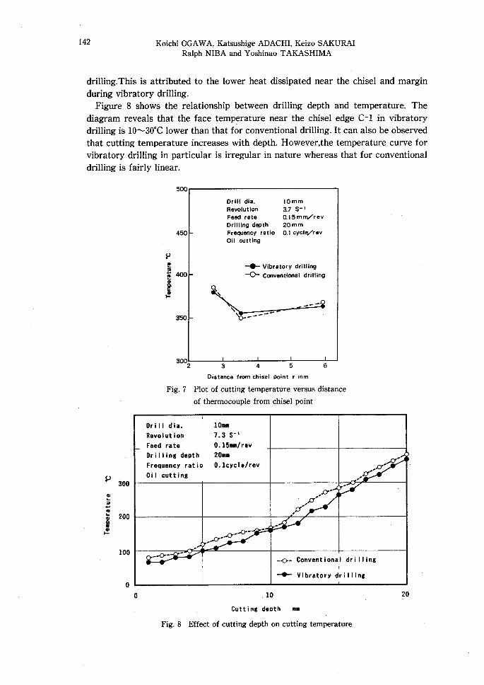
perfomed. Fig. 7 is a plot of distance from chisel point against temperature.
Temperature readings at the face were taken at a drilling depth of 20mm at three
different points from the chisel point.
As it can be seen' in the diagram in Fig. 7 the face temperature for both drilling
methods is higher near the chisel edge C-1 and margin C-3 than the central portion
C-2. A close examination of the diagram also reveals that the face temperature near
the chisel point and margin are lower for vibratory drilling than conventional
142 Koichi OGAWA, Katsushige ADACHI, Keizo SAKURAI Ralph NIBA and Yoshinao TAKASHIMA
drilling.This is attributed to the lower heat dissipated near the chisel and margin
during vibratory drilling.
Figure 8 shows the relationship between drilling depth and temperature. The
diagram reveals that the face temperature near the chisel edge C-1 in vibratory
drilling is 10'v30℃ lower than that for conventional drilling. It can・also be observed
that cutting temperature increases with depth. However,the temperature curve for
vibratory drilling in particular is irregular in nature whereas that for conventional
drilling is fairly linear.
500
450
9eg 4co
gR
350
300
Rts
DrM dia.Revolution
Feed reteDritling depth
Frequency ratio
O" cutting
s
10mm3.7 S-i
O.15mrn/rev20 mmO.1 cyclofrev
- Vibratory drilling
-'(>- Conventional drilting
N5 .. ..--- -
-. ..D
P 3002
etse 2oo
2,.e.
100
o
Fig. 7
Oistance from ehisel point r mm
Plot of cutting temperature versus distance
of thermocouple from chisel point
Drieldia.
Revolution
Feedrate
10mm
7.3S-iO.15mmlrev
Drillingdepth
Frequencyratio
eitcutting
20mm
O.lcycle/revte"
tl
.q'C'
"t
D'"t
."'
'
.D.".Dp
'
'
'
.-O・-'-o- Conventiona ldrilling
Vibratory・tdri1ling
o
Fig. 8
10
Cutting depth mm
Effect of cutting depth on cutting temperature
20

143
Analysis of Cutting 71gmperature of Drill・ Pbint
The irregular temperature curve obtained during vibratory drilling is believed to
be due to the pulsating effect of the vibratory shocks on the cutting edge. While the
drop in temperature can be attributed to improved coolant penetration as a result of
the vibration enabling the coolant to reach the cutting edge thereby curbing wear of
the cutting edges. The reduction in tool wear and cutting forces (static components)
during vibratory drilling is in good agreement with this observation.
4. Analysis of cutting edge temperature by finite element analysis
As it was previously elaborated, the localized temperature at the drill face can be
measured. However,the entire cutting edge temperature is exceptionally difficult to
measure due to the three-dimensional geometry of the drill point. Finite element
analysis is effective in tackling a task of this nature. Surprisingly, there is as yet no
study incorporating the finite element method in drill cutting temperature analysis
despite the conveniences it embodies.
Thus, the finite element method was employed by the authors to theoretically
analyse the cutting edge temperature in conventional drilling. As previously pointed
out, the theoretical analysis of the cutting edge temperature on a three-dimensional
basis entails a lot of difficulties. As a result, in the foregoing analysis attention is
paid to the case involving the formation of continuous chips, which is conventional
drilling.
4. 1 Technique of drill point temperature analysis
The technique leading to an understanding of the drill face temperature distribu-
tion advanced by Shirai et al. entails the solving of unsteady state heat conduction
equations to derive the final steady state temperature distribution. However, in a
case involving the continous ejection of chips, the temperature distribution is thought
to be unsteady due to heat dissipation from within the material. Thus, if initially
after a fixed time has elapsed this technique is treated as a steady state problem it
would be more practical from the viewpoint of reduced computation time. Thus, in
the foregoing analysis, the ordinary differential equation for unsteady state heat
conduction (equation 1) was solved using the finite element method.
x.s<72T+ip-pc OaTt =o (1)
where T is the temperrature, tis the time, Q is the internal heat dissipation ratio,
p, x and c are respectively density, thermal conductivity and specific heat of the
material.
Unlike the three dimensional cutting action of tool bits, the flow of heat along the
cutting edge during the three dimensional cutting action of drills cannot be neglected.
In addition, in the case of drills the flow of heat from chips to the drill has to be
considered, viz, heat conduction and heat velocity boundary conditions have to be
also given consideration. However, since it is impossible in a strict sense to derive

144 Koichi OGAWA, Katsushige ADACHI, Keizo SAKURAI Ralph NIBA and Yoshinao TAKASHIMA
the heat distribution over an entire drill, equation (1) was idealized by finite element
method in cases where provision for temperature T is given as a boundary condition
for steady state heat conduction and the division of the drill point into elements was
implemented. The temperature distribution in an element is depicted by equation (2).
n T( t[,y, z:t) =2 1V} (x;y,2) ¢i (t) (2) i--1
where All・ (x;y,z) is the shape function of the element; dii(t) is the temperature at
node i at time t and n is the number of nodes in the elemerit. A further idealization
of equation (2) yields the finite element equation (3) given by
(Kmn) {g6n}= {Rm}+{Sm} (3) The computer program for three-dimensional heat conduction analysis by Yagawa
et al. was used as reference.
4. 2 Finite element idealization
The drill has a twisted flute and since the drill point thins out toward the tip, it is
extremely difficult to truly perform the three-dimensional idealization of the drill
point, Thus, in this analysis the drill point was divided into surfaces or sections in a
perpendicular directon to the drill axis and the various sections were assembled,
creating a model as shown in Fig. 9. The idealized model is an isoparametric
hexagon with each element having eight nodes. It is desirable for all the divided
sections to have the same number of elements but since the drill point thins out
toward the tip, reduction of the number of elements on each section was adopted.
Furthermore, because the chisel cannot be associated with finite elements, the
surface O.lmm below the chisel was designated the first section and the surface 4.
9mm from the drill tip was divided into 15 sections (denoted A to P making
altogether 16 sections) . Next, each section was idealized into rectangular elements.
The Z coordinate of each section is shown in Table 1. An idealized model is given
in Fig. 10.
It should be mentioned that section L to section P lie on the same surface. An
assembled model of section A to section L is depicted in Fig. 11, there are all
together 2880 finite elements and 3542 nodes in this model. The finite element mesh
diagrams of the drill face(a)and flank(b)at a point 3mm from the drill tip are shown
in Fig. 12.
z
.
' v, s
'
N1
lsNNNN,
Fig. 9 Diagram showing sectioned surface
perpendicular to drill axis

145
Table
Analysis of Cbetti,rg Tlamperainre of Dri'll Pbint
1 Distance of sections from the chisel point in a plane
perpendicular to the drill axis
Section Z-coordinate(mm)
Section Z-coordinate(mm)
A O.1 I 2.4
B O.3 J 2.7
c O.6 K 3.0
D O.9 L 3.3
E 1.2 M 3.7
F 1.5 N 4.1
G 1.8 o 4.5
H 2.1 P 4.9
Fig. 10 Finite element idealization of
section F (Total No. of nodes
=121 ; elements=100)
Fig. 11 An assembled model of section
A'"-L
,
Figr
twtting edge
(a)
12 Finite elementi
Cutting edge
(b)
dealization of drill flank and face

146 Koichi OGAWA, Katsushige ADACHI, Keizo SAKURAI Ralph NIBA and Yoshinao TAKASHIMA
4. 3 Boundary conditions
The following procedure was used to apply the boundary conditions employed in
the analysis. First of all, pre-recorded values of the face temperature from the
face temperature experiment were recorded and then the chisel and margin tem-
perature(maximum temperature)within each surface was held constant while all
other boundary conditions were specified as radiation boundary conditions. The
chisel and margin temperatures were measured by inserting sheathed thermocouples
in the workpiece at the portions shown in the diagram in Fig. 13. Consideration was
given to the temperature value used as boundary condition because of temperature
differences at the various outer corners. Values for gc and x used in the analysis,
are respectively 7.82mg/nf, O.536KJ/Kg ' K and 42.6W/m ' K.
tt/.
-4. tl
× -t
,'liS>,5
f
x.. 1.7
so
gom
:.
:k..
,-
:I--
l-Ietll
,
1'
::
, ,
Thermoco'up
Workpiece
Fig. 13 Position of thermocouple in workpiece
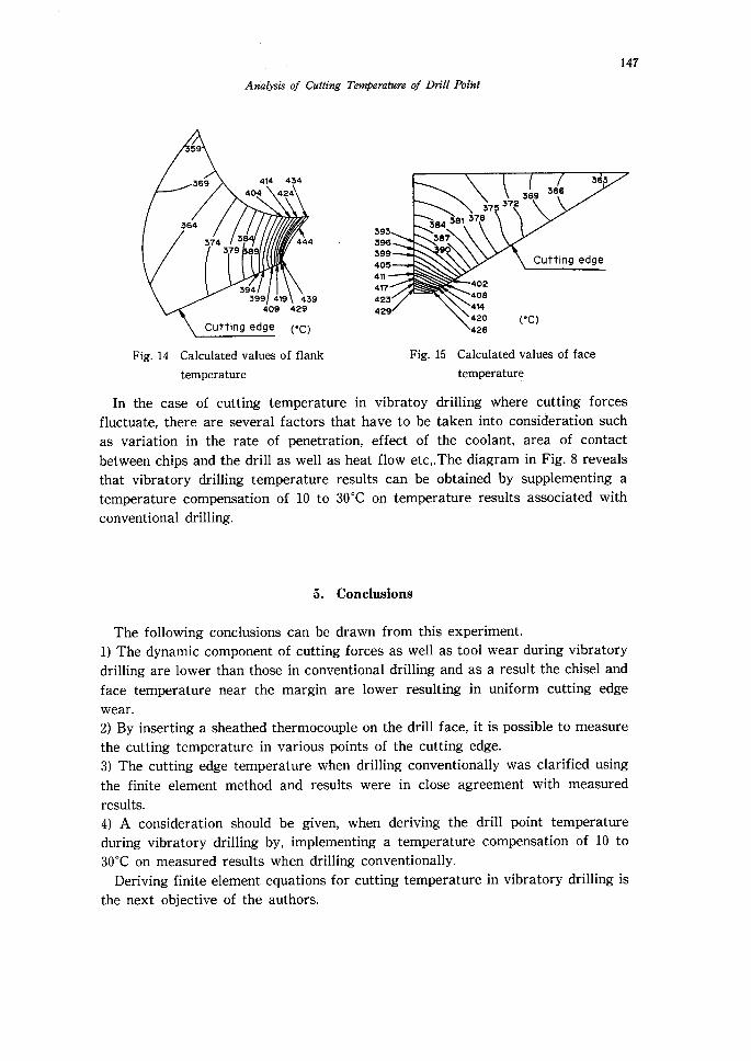
4. 4 Results of numerical analysis and comparison with measured results
The calculated results of the isothermal temperature distribution within the drill
face and flank are shown in the diagrams in Fig. 14 and 15. As was previously
emphasized, readings were taken at a point 3mm from the drill tip. A look at the
temperature slopes in the face temperature distribution diagram reveal the direc-
tion of chip flow while, the temperature slopes in the flank diagram leads to an
understanding of the nature of heat generation at the chisel. Comparing these
results with the measured values in the drill face reVeal that the temperature
difference with drill C-3 was 150C,while the temperature difference with drills C-1
and C-2 was 80C. That is, the numerical values are higher than measured values.
147
An'alysiS of Cutting Tlampevature of Drill Pbin' t
5
569
564
414 454404 424
58574 579 89
594 599 419 409
edge
444
Cutting
Fig. 14 Calculated values of flank
temperature
In the case of cutting
fluctuate, there are several factors
as variation in the rate of
between chips and the drill as well
that vibratory drilling temperature
temperature compensation of 10 to
conventional drilling.
459429
(eC)
595596599405411
417
425429
581584
587
90
572 575578
566569
565
Cutting edge
Fig.
temperature in vibratoy
that have to be
penetration, effect of
as heat flow etc,.The diagram
results can be
30eC on temperature
402 4oe 414 420 (oC). 426
15 Calculated values of face
temperature
drilling where cutting forces
taken into consideration such
the coolant, area of contact
in Fig. 8 reveals
obtained by supplementing a
results associated with
5. Conclusions
The following conclusions can be drawn from this experiment.
I) The dynamic component of cutting forces as well as tool wear during vibratory
drilling are lower than those in conventional drilling and as a result the chisel and
face temperature near the margin are lower resulting in uniform cutting edge
wear.2) By inserting a sheathed thermocouple on the drill face, it is possible to measure
the cutting temperature in various points of the cutting edge.
3) The cutting edge temperature when drilling conventionally was clarified using
the finite element method and results were in close agreement with measured
results.
4) A consideration should be given, when deriving the drill point temperature
during vibratory drilling by, implementing a temperature compensation of 10 to
300C on measured results when drilling conventionally.
Deriving finite element equations for cutting temperature in vibratory drilling is
the next objective of the authors.

148
1)2)
3)4)
5)
6)
7)
8)
9)
Koichi OGAWA, Katsushige ADACHI, Keizo SAKURAI Ralph NIBA and Yosliinao TAKASHIMA
References
M. Tueda, K. Hasegawa: Transaction of the JSME, 28, 384 (1962).
S. Zaima, Y. Suzuki, H. Okushima and S. Yamada : Journal of Japan Institute of Light Metals,
31, 341 (1981).
K. Okuahima, Y. Itagaki : Journal of the Japan Society of Precision Engineering, 36, 1 (1970).
K. Adachi, K. Ogawa, N. Arai, H. Igaki : Journal of Japan Institute of Light Metals, Vol.40, No.
2, 88 (1990).
K. Adachi, K. Ogawa. N. Arai, K. Okita, R. Niba : Bull. Japan Soc. of Engg., Vol.24, No.3, 200
(1990).
K. Ogawa, K. Adachi, K. Sakurai, R.,Niba, Y. Takashima : Bull. of Univ. of Osaka Prefecture,
Vol.39, No.1, 95 (1990).
K. Adachi, K. Ogawa, N. Arai, H. Igaki : Journal of Japan Institute of Light Metals, Vol.40, No.
3, 171 (1990).
N. Arai, K. Adachi, M. Nakamura, K. Ogawa : Proceedings of The 3rd Sino-Japan Conference
on Ultraprecision Machining, Cll-Ol (1990).
M. Yagawa, A FEM Guide for Flow and Head Conduction, Baifukan, 223 <1983).