1

Title 1

Bending the curve of terrestrial biodiversity needs an integrated strategy 2

3

Summary paragraph 4

Increased efforts are required to prevent further losses of terrestrial biodiversity and the ecosystem 5

services it provides1,2. Ambitious targets have been proposed, such as reversing the declining trends 6

in biodiversity3 – yet, just feeding the growing human population will make this a challenge4. We use 7

an ensemble of land-use and biodiversity models to assess whether (and if so, how) humanity can 8

reverse terrestrial biodiversity declines due to habitat conversion, a major threat to biodiversity5. 9

We show that immediate efforts, consistent with the broader sustainability agenda but of 10

unprecedented ambition and coordination, may allow to feed the growing human population while 11

reversing global terrestrial biodiversity trends from habitat conversion. If we decide to increase the 12

extent of land under conservation management, restore degraded land, and generalize landscape-13

level conservation planning, biodiversity trends from habitat conversion could become positive by 14

mid-century on average across models (confidence interval: 2042-2061), but not for all models. Food 15

prices could increase and, on average across models, almost half (confidence interval: 34-50%) of 16

future biodiversity losses could not be avoided. However, additionally tackling the drivers of land-17

use change may avoid conflict with affordable food provision and reduces the food system’s 18

environmental impacts. Through further sustainable intensification and trade, reduced food waste, 19

and healthier human diets, more than two thirds of future biodiversity losses are avoided and the 20

biodiversity trends from habitat conversion are reversed by 2050 for almost all models. Although 21

limiting further loss will remain challenging in several biodiversity-rich regions, and other threats, 22

such as climate change, must be addressed to truly reverse biodiversity declines, our results show 23

that bold conservation efforts and food system transformation are central to an effective post-2020 24

biodiversity strategy. 25

2

Main text 26

27

Terrestrial biodiversity is decreasing rapidly1,2 as a result of human pressures, largely through habitat 28

loss and degradation due to the conversion of natural habitats to agriculture and forestry5. 29

Conservation efforts have not halted the trends6 and land demand for food, feed and energy 30

provision is increasing7,8, putting at risk the myriad of ecosystem services people depend upon9–11. 31

32

Ambitious targets for biodiversity have been proposed, such as halting and even reversing the 33

currently declining trends3,12 and conserving half of the Earth13. However, evidence is lacking on 34

whether such biodiversity targets can be achieved, given that they may conflict with food provision4 35

and other land uses. As a step towards developing a strategy for biodiversity that is consistent with 36

the sustainable development agenda, we have used a multi-model ensemble approach14,15 to assess 37

whether and how future biodiversity trends from habitat loss and degradation can be reversed, 38

while still feeding the growing human population. 39

40

We designed seven scenarios to explore pathways towards reversing the declining biodiversity 41

trends (Table 1; Methods), based on the Shared Socioeconomic Pathway (SSP) scenario 42

framework16. The Middle of the Road SSP2 defined our baseline scenario (denoted as BASE) for 43

future drivers of habitat loss. In six additional scenarios we considered different combinations of 44

supply-side, demand-side and conservation efforts towards reversing biodiversity trends: these were 45

based on the Green Growth SSP1 scenario, augmented by ambitious conservation assumptions 46

(Extended Data Fig. 1), and culminated in the Integrated Action Portfolio (IAP) scenario which 47

includes all efforts. 48

49

Because of the uncertainties inherent in estimating how drivers will change and how these changes 50

will affect biodiversity, we used an ensemble approach to model biodiversity trends for each 51

3

scenario. First, we used the land-use components of four Integrated Assessment Models (IAMs) to 52

generate four spatially and temporally resolved projections of habitat loss and degradation for each 53

scenario (Methods). These IAM outputs were then evaluated by eight biodiversity models (BDMs) to 54

project nine biodiversity indicators (BDIs, each defined as one biodiversity metric estimated by one 55

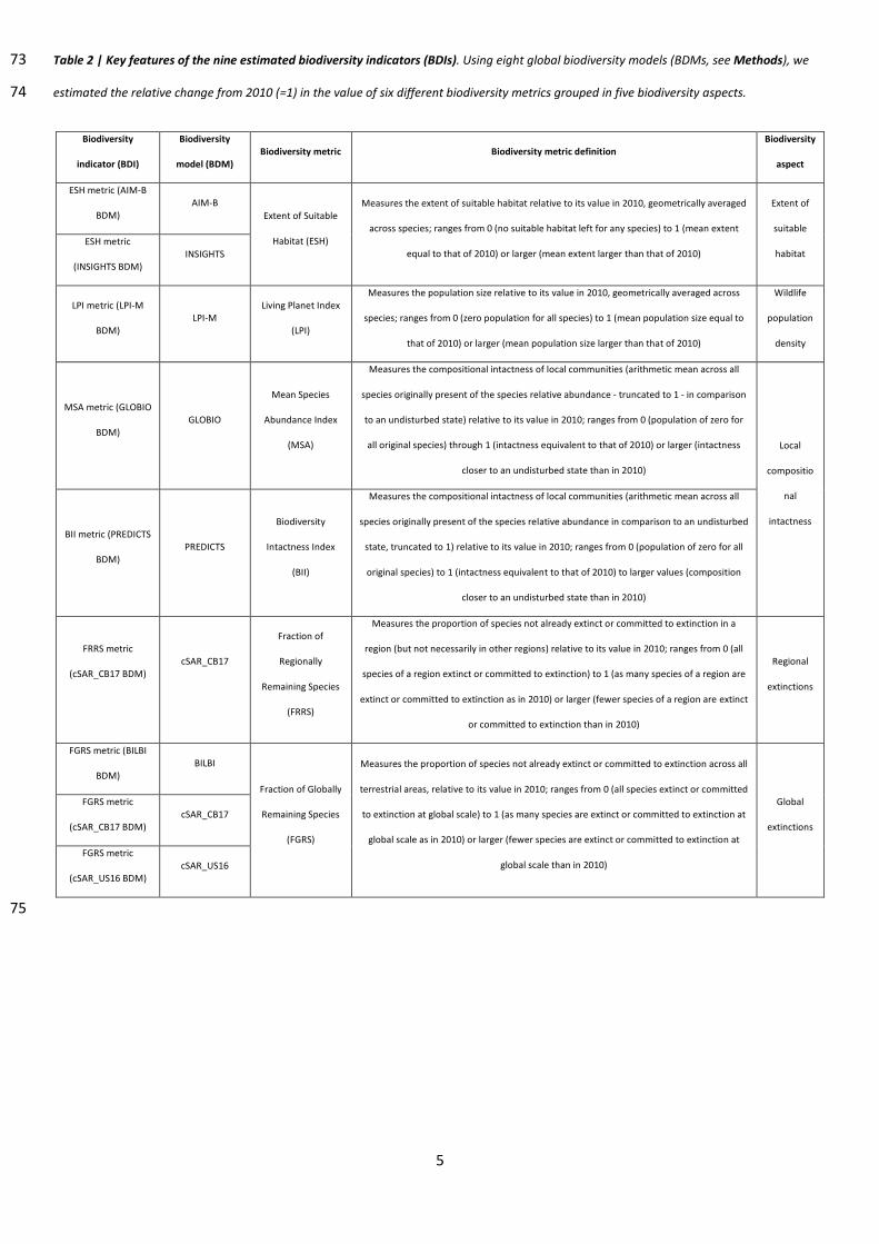
BDM; Table 2) describing trends in five aspects of biodiversity: extent of suitable habitat, wildlife 56

population density, local compositional intactness, regional species extinctions, and global species 57

extinctions. The BASE and IAP scenarios were projected for an ensemble of 34 combinations of IAMs 58

and BDIs; the other five scenarios were evaluated for a subset of seven BDIs for each IAM (ensemble 59

of 28 combinations, see Methods). To obtain more robust insights, we performed bootstrap 60

resampling17 of the ensembles (10,000 samples with replacement, see Methods). We used state-of-61

the-art models of terrestrial biodiversity for global scale and broad taxonomic coverage, however, 62

we note that more sophisticated modeling approaches – currently hard to apply at such scales – 63

might provide more accurate estimates at smaller scales18. While we estimate future biodiversity as 64

affected by future trends in the largest threat to biodiversity to date (habitat destruction and 65

degradation), we note that more accurate projections of future biodiversity trends should account 66

for additional threats to biodiversity, such as climate change or invasive alien species. 67

68

4

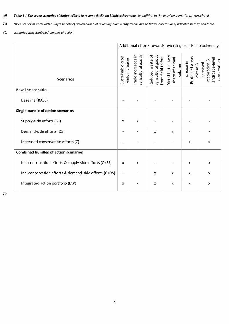
Table 1 | The seven scenarios picturing efforts to reverse declining biodiversity trends. In addition to the baseline scenario, we considered 69

three scenarios each with a single bundle of action aimed at reversing biodiversity trends due to future habitat loss (indicated with x) and three 70

scenarios with combined bundles of action. 71

Scenarios

Additional efforts towards reversing trends in biodiversity

Sust

aina

ble

crop

yi

eld

incr

ease

s

Trad

e in

crea

ses i

n ag

ricul

tura

l goo

ds

Redu

ced

was

te o

f ag

ricul

tura

l goo

ds

from

fiel

d to

fork

Diet

shift

to lo

wer

sh

are

of a

nim

al

calo

ries

Incr

ease

in

Prot

ecte

d Ar

eas

exte

nt &

Incr

ease

d re

stor

atio

n &

la

ndsc

ape-

leve

l co

nser

vatio

n

Baseline scenario

Baseline (BASE) - - - - - -

Single bundle of action scenarios

Supply-side efforts (SS) x x - - - -

Demand-side efforts (DS) - - x x - -

Increased conservation efforts (C) - - - - x x

Combined bundles of action scenarios

Inc. conservation efforts & supply-side efforts (C+SS) x x - - x x

Inc. conservation efforts & demand-side efforts (C+DS) - - x x x x

Integrated action portfolio (IAP) x x x x x x

72

5

Table 2 | Key features of the nine estimated biodiversity indicators (BDIs). Using eight global biodiversity models (BDMs, see Methods), we 73

estimated the relative change from 2010 (=1) in the value of six different biodiversity metrics grouped in five biodiversity aspects. 74

Biodiversity

indicator (BDI)

Biodiversity

model (BDM) Biodiversity metric Biodiversity metric definition

Biodiversity

aspect

ESH metric (AIM-B

BDM) AIM-B

Extent of Suitable

Habitat (ESH)

Measures the extent of suitable habitat relative to its value in 2010, geometrically averaged

across species; ranges from 0 (no suitable habitat left for any species) to 1 (mean extent

equal to that of 2010) or larger (mean extent larger than that of 2010)

Extent of

suitable

habitat ESH metric

(INSIGHTS BDM) INSIGHTS

LPI metric (LPI-M

BDM) LPI-M

Living Planet Index

(LPI)

Measures the population size relative to its value in 2010, geometrically averaged across

species; ranges from 0 (zero population for all species) to 1 (mean population size equal to

that of 2010) or larger (mean population size larger than that of 2010)

Wildlife

population

density

MSA metric (GLOBIO

BDM) GLOBIO

Mean Species

Abundance Index

(MSA)

Measures the compositional intactness of local communities (arithmetic mean across all

species originally present of the species relative abundance - truncated to 1 - in comparison

to an undisturbed state) relative to its value in 2010; ranges from 0 (population of zero for

all original species) through 1 (intactness equivalent to that of 2010) or larger (intactness

closer to an undisturbed state than in 2010)

Local

compositio

nal

intactness BII metric (PREDICTS

BDM) PREDICTS

Biodiversity

Intactness Index

(BII)

Measures the compositional intactness of local communities (arithmetic mean across all

species originally present of the species relative abundance in comparison to an undisturbed

state, truncated to 1) relative to its value in 2010; ranges from 0 (population of zero for all

original species) to 1 (intactness equivalent to that of 2010) to larger values (composition

closer to an undisturbed state than in 2010)

FRRS metric

(cSAR_CB17 BDM)

cSAR_CB17

Fraction of

Regionally

Remaining Species

(FRRS)

Measures the proportion of species not already extinct or committed to extinction in a

region (but not necessarily in other regions) relative to its value in 2010; ranges from 0 (all

species of a region extinct or committed to extinction) to 1 (as many species of a region are

extinct or committed to extinction as in 2010) or larger (fewer species of a region are extinct

or committed to extinction than in 2010)

Regional

extinctions

FGRS metric (BILBI

BDM) BILBI

Fraction of Globally

Remaining Species

(FGRS)

Measures the proportion of species not already extinct or committed to extinction across all

terrestrial areas, relative to its value in 2010; ranges from 0 (all species extinct or committed

to extinction at global scale) to 1 (as many species are extinct or committed to extinction at

global scale as in 2010) or larger (fewer species are extinct or committed to extinction at

global scale than in 2010)

Global

extinctions

FGRS metric

(cSAR_CB17 BDM) cSAR_CB17

FGRS metric

(cSAR_US16 BDM) cSAR_US16

75

6

Reversing biodiversity trends by 2050 76

Without further efforts to counteract habitat loss and degradation, we projected that global 77

biodiversity will continue to decline (BASE scenario; Fig. 1). Rates of loss over time for all nine BDIs in 78

2010-2050 were close to or greater than those estimated for 1970-2010 (Extended data 79

Extended Data Table 1). For various biodiversity aspects, on average across IAM and BDI 80

combinations, peak losses over the 2010-2100 period were: 13% (range: 1-26%) for the extent of 81

suitable habitat, 54% (range: 45-63%) for wildlife population density, 5% (range: 2-9%) for local 82

compositional intactness , 4% (range: 1-12%) for global extinctions, and 4% (range: 2-8%) for 83

regional extinctions (Extended Data Table 1). Percentage losses were greatest in biodiversity-rich 84

regions (Sub-Saharan Africa, South Asia, South East Asia, the Caribbean and Latin America; Extended 85

Data Fig. 2). The projected future trends for habitat loss and degradation and its drivers8,16, 86

biodiversity loss7,8, and variation in loss across biodiversity aspects7,19,20 are consistent with those 87

reported in other studies1 (Extended Data Fig. 2-5; Supp. discussion 1). 88

89

In contrast, ambitious integrated efforts could minimize further declines and reverse biodiversity 90

trends driven by habitat loss (IAP scenario; Fig. 1). In the IAP scenario, biodiversity loss was halted by 91

2050 and was followed by recovery for all IAM and BDI combinations except for one (IMAGE IAM x 92

GLOBIO-MSA BDI). This reflects reductions in habitat loss and degradation and its drivers, and 93

restoration of degraded habitats in this scenario (Extended Data Fig. 3-5; Supp. discussion 1). 94

Although global biodiversity losses are unlikely to be halted by 20206, rapidly stopping the global 95

biodiversity decline due to habitat loss is a milestone on the path to more ambitious targets. 96

97

Uncertainties in both future land use and its impact on biodiversity are significant, reflecting 98

knowledge gaps15. To maximize the robustness of conclusions in the face of these uncertainties, we 99

used a strategy with three main elements. First, as recommended by the IPBES15, we conduct a 100

multi-model assessment, building on the strengths and mitigating the weaknesses of several 101

7

individual IAMs and BDMs to characterize uncertainties, understand their sources and identify 102

results that are robust to these uncertainties. Looking at one BDI across multiple IAMs (e.g., ribbons 103

in individual panels of Fig. 1), or comparing two BDIs informing on the same biodiversity aspect (e.g., 104

MSA and BII BDIs in Fig. 1 c.) illuminates uncertainties stemming from individual model features such 105

as initial condition, internal dynamics and scenario implementation. This shows, for example, that 106

differences between IAMs in the initial area of grassland suitable for restoration and in the intensity 107

of restoration efforts induce large uncertainties in biodiversity trends in all scenarios involving 108

increased conservation efforts (C, C+SS, C+DS and IAP scenarios, Supp. discussion 2). Similarly, 109

differences between BDMs in the timing of biodiversity recovery under restoration introduces 110

further uncertainties, as do differences in taxonomic coverage and input data source between BDMs 111

modeling the same BDI (Supp. discussion 2). 112

113

Second, rather than the absolute values of BDIs, we focus on the direction and inflexion in their 114

relative change over time and their response to differences in land-use change outcomes across 115

scenarios. This choice emphasizes aspects of biodiversity outcomes that are more directly 116

comparable across multiple models and means comparisons are less impacted by model-specific 117

differences and biases. We also used the most recent versions of BDMs that are still developing – for 118

example, the PREDICTS implementation of BII used here21 better captures compositional turnover 119

caused by land-use change than did an earlier implementation22. All BDMs remain affected by 120

uncertainty in the initial land-use distribution, especially the spatial distribution of current forest and 121

grassland management, which varies across IAMs and causes estimates of all BDIs for the year 2010 122

to differ significantly among IAMs. Because these initial differences between IAMs persist across 123

time horizons and scenarios, the direction and amplitude of projected relative changes in indicator 124

values are more informative than their absolute values across the ensemble. 125

126

8

Third, we used bootstrap resampling with replacement to obtain confidence intervals of ensemble 127

statistics and limit the influence of any particular model on the key results (Methods). However, our 128

approach does not cover part of the overall uncertainty, stemming from either individual models 129

(e.g., related to input parameter uncertainty) or limitations common to most models implemented 130

in this study, such as the rudimentary representation of relationships between biodiversity and land-131

use intensity (see Supp. discussion 2, and Methods for more information on the evaluation of 132

individual BDMs). 133

134

9

135

Fig. 1 | Estimated recent and future global biodiversity trends resulting from land-use change, with and without coordinated efforts to 136

reverse trends. Panels a-e depict the trends for the five aspects of biodiversity, resulting from changes in nine biodiversity indicators (BDIs; 137

individual sub-panels, see Table 2). BDI values are shown as differences from the 2010 value (=1); a value of -0.01 means a 1% loss in: the 138

extent of suitable habitat (panel a), the wildlife population density (panel b), the local compositional intactness (panel c), the regional number 139

of species (panel d) or the global number of species (panel e). BDI values are projected in response to land-use change derived from one source 140

over the historical period (1970-2010, black line; 2010 is indicated with a vertical dashed line) and from four Integrated Assessment Models 141

(IAMs: AIM, GLOBIOM, IMAGE and MAgPIE; thick lines display the mean across models while ribbons display the range across models) for the 142

baseline BASE scenario (grey) and Integrated Action Portfolio IAP scenario (yellow, see Table 1) over the future period (2010-2100).143

10

Contribution of different interventions 144

To understand the contribution of different strategies, we analyzed the BDI trends projected for all 145

seven scenarios (see Table 1) for an ensemble of 28 BDI and IAM combinations, as shown in Fig. 2a 146

for the MSA BDI and Extended Data Fig. 6 for other BDIs. We focused on ensemble statistics for 147

three outcomes (Fig. 2b; Extended Data Table 2): the date of peak loss (date at which the BDI value 148

reached its minimum over the 2010-2100 period); the share of future peak loss that could be 149

avoided, compared to the BASE scenario; and the speed of recovery after the peak loss (the recovery 150

rate after peak loss, relative to the rate of decline over the historical period, see Methods). 151

152

Our analysis shows that a bold conservation plan is crucial for halting biodiversity declines and 153

setting ecosystems onto a recovery path3. Increased conservation efforts (C scenario) was the only 154

single bundle of action scenario leading on average across the ensemble to both a peak in future 155

biodiversity losses before the last quarter of the 21st century (mean and 95% CI of the average date 156

of peak loss ≤ 2075) and large reductions in future losses (mean and 95% CI of the average 157

reductions ≥ 50%). On average across the ensemble, the speed of biodiversity recovery after peak 158

loss was slow in Supply-Side (SS) and Demand-Side (DS) scenarios, but much faster when also 159

combining increased conservation and restoration (in C, C+SS, C+DS and IAP scenarios), with a larger 160

amount of reclaimed managed land (Extended Data Fig. 4). Our IAP scenario involve restoring 4.3-161

14.6 million km2 of land by 2050, requiring the Bonn Challenge target (3.5 million km2 by 2030) to be 162

augmented by higher targets for 2050. 163

164

However, efforts to increase both the management and the extent of protected areas – to 40% of 165

terrestrial area, based on wilderness areas and Key Biodiversity Areas – and to increase landscape-166

level conservation planning efforts in all terrestrial areas (C scenario; Methods) were insufficient on 167

average to avoid >50% of the losses projected in the BASE scenario in many biodiversity-rich regions 168

(Extended Data Fig. 7). Furthermore, the slight decrease in the global crop price index projected on 169

11

average across IAMs in the BASE scenario was reversed in the C scenario (Extended Data Fig. 8). 170

Without transformation of the food system, bolder conservation efforts would be conflict with 171

future food provision, given the projected technological developments in agricultural productivity 172

across models (Supp. discussion 3). 173

174

In contrast, a deeper food system transformation, relying on feasible supply-side and demand-side 175

efforts as well as increased conservation efforts (IAP scenario; Supp. discussion 3), would greatly 176

facilitate the reversal of biodiversity trends, reduce the trade-offs emerging from siloed policies, and 177

offer broader benefits. On average across the ensemble, ≥67% of future peak losses were avoided 178

for 96% (95% CI: 89-100%) of IAM and BDI combinations in the IAP scenario, in contrast to 43% (95% 179

CI: 25-61%) in the C scenario (see Extended Data Table 2). Similarly, across the ensemble, 180

biodiversity trends were reversed by 2050 for 96% (95% CI: 89%-100%) of IAM and BDI combinations 181

in the IAP scenario vs. 61% (95% CI: 43%-79%) in the C scenario. Integrated efforts thus alleviate 182

pressures on habitats (Extended Data Fig. 5) and reverse biodiversity trends from habitat loss 183

decades earlier than strategies that allow habitat losses followed by restoration (Extended Data Fig. 184

7). Integrated efforts might also mitigate the trade-offs between regions and exploit 185

complementarities between interventions: for example, increased agricultural intensification and 186

trade may limit agricultural land expansion at the global scale, but induce expansion at a regional 187

scale unless complemented with conservation efforts23,24. We found spatially contrasted – and 188

sometimes regionally negative – impacts of various interventions, but the number of regions in 189

favorable status increased with integration efforts (Extended Data Figure 7) . Finally, integrated 190

strategies have benefits other than just enhancing biodiversity: dietary transitions alone have 191

significant benefits for human health25, and integrated strategies may also increase food availability, 192

reverse future trends in greenhouse gas emissions from land use, and limit increases in the impact of 193

land use on the water and nutrient cycles (Extended Data Fig. 8; Supp. discussion 4). 194

195

12

196

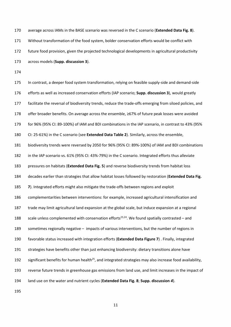
Fig. 2 | Contributions of various efforts to reverse land-use change-induced biodiversity trends. Future actions towards reversing biodiversity 197

trends vary across seven scenarios (BASE, SS, DS, C, C+SS, C+DS and IAP), indicated by different colors. In panel a, the line for each future 198

scenario represents the mean across four IAMs and the ribbon represents the range across four IAMs of future changes (compared to 2010) for 199

one illustrative biodiversity metric (MSA) estimated by one biodiversity model (GLOBIO). For the historical period, the black line represents the 200

changes projected in the same biodiversity metric for the single land-use dataset considered over this period. Symbols display the estimated 201

changes by 2100 for individual IAMs. Panel b displays estimates of the distribution across combinations of BDIs and IAMs, for each scenario, of: 202

the date of the 21st century minimum (date of peak loss, left sub-panel); the proportion of peak biodiversity losses that could be avoided 203

compared to the BASE scenario (middle sub-panel); and the speed of recovery after the minimum has been reached (right sub-panel, 204

normalized by the historical speed of change, so that a value of -1 means recovery at the speed at which biodiversity losses took place in 1970-205

2010, and values lower than -1 indicate a recovery faster than the 1970-2010 loss). Values are estimated from 10,000 bootstrap samples from 206

the original combination of BDIs and IAMs: in each boxplot, the thick vertical bar indicates the mean estimate (across bootstrap samples) of the 207

mean value (across BDI and IAM combinations), the box indicates the 95% confidence interval of the mean value, and the horizontal lines 208

indicate the mean estimates (across bootstrap samples) of the 2.5th and 97.5th quantiles (across BDI and IAM combinations). In each boxplot, 209

the estimates are based on bootstrap samples with N=28 (7 BDIs x 4 IAMs), except for the right sub-panel, in which N ≤ 28, as the speed of 210

recovery after peak loss is not defined if the peak loss is not reached before 2100. 211

13

Discussion and conclusions 212

Our study suggests ways of resolving key trade-offs associated with bold actions for terrestrial 213

biodiversity4,26. Actions in our IAP scenario address the largest threat to biodiversity – habitat loss 214

and degradation – and are projected to reverse declines for five aspects of biodiversity. These 215

actions may be technically possible, economically feasible and consistent with broader sustainability 216

goals, but designing and implementing policies that enables such efforts will be challenging and will 217

demand concerted leadership (Supp. discussion 3). In addition, reversing declines in other 218

biodiversity aspects (e.g., phylogenetic and functional diversity) might require different spatial 219

allocation of conservation and restoration actions, and possibly higher areal increase (Supp. 220

discussion 5). Similarly, other threats (e.g., climate change, biological invasions) currently affect two 221

to three times fewer species than land-use change at the global scale5, but can be more important 222

locally, can have synergistic effects, and will increase in global importance in the future. Therefore, a 223

full reversal of biodiversity declines will require additional interventions, such as ambitious climate 224

change mitigation that exploits synergies with biodiversity rather than further eroding biodiversity. 225

Nevertheless, even if the actions explored in this study are insufficient, they will remain essential for 226

reversing terrestrial biodiversity trends. 227

228

The need for transformative change and responses that simultaneously address a nexus of 229

sustainability goals was recently documented by the Intergovernmental Science-Policy Platform on 230

Biodiversity and Ecosystem Services1,2. Our study complements that assessment by shedding light on 231

the nature, ambition and complementarity of actions required to reverse the decline of global 232

biodiversity trends from habitat loss, with direct implications for the international post-2020 233

biodiversity strategy. Reversing biodiversity trends – an interpretation of the 2050 Vision of the 234

Convention on Biological Diversity – requires the urgent adoption of a conservation plan that retains 235

the remaining biodiversity and restores degraded areas. Our scenarios feature an expansion to up to 236

40% of terrestrial areas with effective management for biodiversity, restoration efforts beyond the 237

14

targets of the Bonn Challenge, and a generalization of land-use planning and landscape approaches. 238

Such a bold conservation plan will conflict with other societal demands from land, unless 239

transformations for sustainable food production and consumption are simultaneously considered. 240

For a successful post-2020 biodiversity strategy, ambitious conservation must be combined with 241

action on drivers of biodiversity loss, especially in the land use sectors. Without an integrated 242

approach that exploits synergies with the Sustainable Development agenda, future habitat losses will 243

at best take decades to restore, and further irreversible biodiversity losses are likely. 244

245

Models and scenarios can help to further outline integrated strategies that build upon contributions 246

from nature to achieve sustainable development. This will however necessitate further research and 247

the development of appropriate practices at the science-policy interface. Future assessments should 248

seek to better represent land-management practices as well as additional pressures on land and 249

biodiversity, such as climate change impact and mitigation, overexploitation, pollution and biological 250

invasions. The upscaling of novel modeling approaches might facilitate such improvements, although 251

it currently faces data and technical challenges18. In addition to innovative model developments and 252

multi-model assessments, efforts are needed to evaluate and report on the uncertainty and 253

performance of individual models. Such efforts however remain constrained by the complexity of 254

natural and human systems and data limitations: for example, the models used in this analysis lack 255

validation, not least because a thorough validation effort would face data and conceptual 256

limitations27. . In such a context, both improved modeling practices (e.g., open source and FAIR 257

principles28, community-wide modeling standards29) and participatory approaches to validation 258

might play a key role in enhancing the usefulness of models and scenarios30. 259

260

15

References 261

1. IPBES. Summary for policymakers of the global assessment report on biodiversity and ecosystem services of 262

the Intergovernmental Science-Policy Platform on Biodiversity and Ecosystem Services. (IPBES secretariat, 263

2019). 264

2. Díaz, S. et al. Pervasive human-driven decline of life on Earth points to the need for transformative change. 265

Science (80-. ). 366, (2019). 266

3. Mace, G. M. et al. Aiming higher to bend the curve of biodiversity loss. Nat. Sustain. (2018). 267

4. Mehrabi, Z., Ellis, E. C. & Ramankutty, N. The challenge of feeding the world while conserving half the planet. 268

Nat. Sustain. 1, 409–412 (2018). 269

5. Maxwell, S. L., Fuller, R. A., Brooks, T. M. & Watson, J. E. M. The ravages of guns, nets and bulldozers. Nature 270

536, 146–145 (2016). 271

6. Tittensor, D. P. et al. A mid-term analysis of progress toward international biodiversity targets. Science (80-. ). 272

346, 241–245 (2014). 273

7. Newbold, T. et al. Global effects of land use on local terrestrial biodiversity. Nature 520, 45 (2015). 274

8. Tilman, D. et al. Future threats to biodiversity and pathways to their prevention. Nature 546, 73–81 (2017). 275

9. Cardinale, B. J. et al. Biodiversity loss and its impact on humanity. Nature 489, 326–326 (2012). 276

10. Steffen, W. et al. Planetary Boundaries: Guiding human development on a changing planet. Science (80-. ). 277

347, (2015). 278

11. Chaplin-Kramer, R. et al. Global modeling of nature’s contributions to people. Science (80-. ). 366, 255–258 279

(2019). 280

12. Van Vuuren, D. P. et al. Pathways to achieve a set of ambitious global sustainability objectives by 2050 : 281

Explorations using the IMAGE integrated assessment model. Technol. Forecast. Soc. Chang. (2015). 282

13. Wilson, E. O. Half-Earth: Our Planet’s Fight for Life. (2016). 283

14. Tebaldi, C. & Knutti, R. The use of the multi-model ensemble in probabilistic climate projections. Philos. Trans. 284

R. Soc. A Math. Phys. Eng. Sci. 365, 2053–2075 (2007). 285

15. IPBES. Summary for policymakers of the methodological assessment of scenarios and models of biodiversity 286

and ecosystem services of the Intergovernmental Science-Policy Platform on Biodiversity and Ecosystem 287

Services. (2016). 288

16

16. Popp, A. et al. Land-use futures in the shared socio-economic pathways. Glob. Environ. Chang. 42, (2017). 289

17. Efron, B. & Tibshirani, R. Statistical Data Analysis in the Computer Age. Science (80-. ). 253, 390–395 (1991). 290

18. Briscoe, N. J. et al. Forecasting species range dynamics with process-explicit models: matching methods to 291

applications. Ecol. Lett. 22, 1940–1956 (2019). 292

19. McRae, L., Deinet, S. & Freeman, R. The diversity-weighted living planet index: Controlling for taxonomic bias 293

in a global biodiversity indicator. PLoS One 12, 1–20 (2017). 294

20. Newbold, T. et al. Has land use pushed terrestrial biodiversity beyond the planetary boundary? A global 295

assessment. Science (80-. ). 353, 288–291 (2016). 296

21. Newbold, T., Sanchez-Ortiz, K., De Palma, A., Hill, S. L. L. & Purvis, A. Reply to ‘The biodiversity intactness 297

index may underestimate losses’. Nat. Ecol. Evol. 3, 864–865 (2019). 298

22. Martin, P. A., Green, R. E. & Balmford, A. The biodiversity intactness index may underestimate losses. Nat. 299

Ecol. Evol. (2019). doi:10.1038/s41559-019-0895-1 300

23. Phalan, B. et al. How can higher-yield farming help to spare nature? Science (80-. ). 351, 450–451 (2016). 301

24. Lambin, E. F. & Meyfroidt, P. Global land use change, economic globalization, and the looming land scarcity. 302

Proc. Natl. Acad. Sci. 108, 3465–3472 (2011). 303

25. Springmann, M. et al. Options for keeping the food system within environmental limits. Nature (2018). 304

doi:10.1038/s41586-018-0594-0 305

26. Pimm, S. L., Jenkins, C. N. & Li, B. V. How to protect half of Earth to ensure it protects sufficient biodiversity. 306

1–8 (2018). doi:10.1126/sciadv.aat2616 307

27. Mouquet, N. et al. Predictive ecology in a changing world. J. Appl. Ecol. 52, 1293–1310 (2015). 308

28. Wilkinson, M. D. et al. Comment: The FAIR Guiding Principles for scientific data management and 309

stewardship. Sci. Data 3, 1–9 (2016). 310

29. Araújo, M. B. et al. Standards for distribution models in biodiversity assessments. Sci. Adv. 5, 1–12 (2019). 311

30. Eker, S., Rovenskaya, E., Obersteiner, M. & Langan, S. Practice and perspectives in the validation of resource 312

management models. Nat. Commun. 9, 1–10 (2018). 313

31. Riahi, K. et al. The Shared Socioeconomic Pathways and their energy, land use, and greenhouse gas emissions 314

implications: An overview. Glob. Environ. Chang. 42, 153–168 (2017). 315

32. Fricko, O. et al. The marker quantification of the Shared Socioeconomic Pathway 2: A middle-of-the-road 316

17

scenario for the 21st century. Glob. Environ. Chang. (2017). doi:10.1016/j.gloenvcha.2016.06.004 317

33. Leclère, D. et al. Towards pathways bending the curve of terrestrial biodiversity trends within the 21st 318

century (v 1.3): update of methods underpinning the article entitled ‘Bending the curve of terrestrial 319

biodiversity needs an integrated strategy’. (2020). 320

34. van Vuuren, D. P. et al. Energy, land-use and greenhouse gas emissions trajectories under a green growth 321

paradigm. Glob. Environ. Chang. 42, 237–250 (2017). 322

35. IUCN & UNEP-WCMC. The World Database on Protected Areas (WDPA) [On-line], downloaded 09/2017. 323

(UNEP-WCMC, 2017). 324

36. BirdLife International. World Database of Key Biodiversity Areas, developed by the KBA Partnership [Accessed 325

05/10/2017]. (2017). 326

37. Allan, J. R., Venter, O. & Watson, J. E. M. Temporally inter-comparable maps of terrestrial wilderness and the 327

Last of the Wild. Sci. Data 4, 1–8 (2017). 328

38. Scholes, R. J. & Biggs, R. A biodiversity intactness index. Nature 434, 45–49 (2005). 329

39. Hudson, L. N. et al. The database of the PREDICTS (Projecting Responses of Ecological Diversity In Changing 330

Terrestrial Systems) project. Ecol. Evol. 7, 145–188 (2017). 331

40. Hurtt, G. et al. Harmonization of global land-use change and management for the period 850–2100 (In prep.). 332

Geosci. Model Dev. 333

41. IUCN. Red List of threatened species version 2017.3, <http://www. iucnredlist.org>. (2017). 334

42. BirdLife International & Handbook of the Birds of the World. Bird species distribution maps of the world. 335

Version 7.0. (2017). 336

43. Harfoot, M. et al. Integrated assessment models for ecologists: The present and the future. Glob. Ecol. 337

Biogeogr. 23, 124–143 (2014). 338

44. Fujimori, S., Masui, T. & Matsuoka, Y. AIM/CGE [basic] manual. (2012). 339

45. Hasegawa, T., Fujimori, S., Ito, A., Takahashi, K. & Masui, T. Global land-use allocation model linked to an 340

integrated assessment model. Sci. Total Environ. 580, 787–796 (2017). 341

46. Havlík, P. et al. Climate change mitigation through livestock system transitions. Proc. Natl. Acad. Sci. U. S. A. 342

111, 3709–14 (2014). 343

47. Stehfest, E. et al. Integrated Assessment of Global Environmental Change with IMAGE 3.0: Model description 344

18

and policy applications. (2014). 345

48. Woltjer, G. et al. The MAGNET model. 148 (2014). 346

49. Popp, A. et al. Land-use protection for climate change mitigation. Nat. Clim. Chang. 4, 1095–1098 (2014). 347

50. Brooks, T. M. et al. Analysing biodiversity and conservation knowledge products to support regional 348

environmental assessments. Sci. Data 3, 160007 (2016). 349

51. Klein Goldewijk, K., Beusen, A., Van Drecht, G. & De Vos, M. The HYDE 3.1 spatially explicit database of 350

human-induced global land-use change over the past 12,000 years. Glob. Ecol. Biogeogr. 20, 73–86 (2011). 351

52. Ohashi, H. et al. Biodiversity can benefit from climate stabilization despite adverse side effects of land-based 352

mitigation. Nat. Commun. 10, 5240 (2019). 353

53. Visconti, P. et al. Projecting Global Biodiversity Indicators under Future Development Scenarios. Conserv. Lett. 354

9, 5–13 (2016). 355

54. Rondinini, C. & Visconti, P. Scenarios of large mammal loss in Europe for the 21st century. Conserv. Biol. 29, 356

1028–1036 (2015). 357

55. Spooner, F. E. B., Pearson, R. G. & Freeman, R. Rapid warming is associated with population decline among 358

terrestrial birds and mammals globally. Glob. Chang. Biol. 24, 4521–4531 (2018). 359

56. Ferrier, S., Manion, G., Elith, J. & Richardson, K. Using generalized dissimilarity modelling to analyse and 360

predict patterns of beta diversity in regional biodiversity assessment. Divers. Distrib. 13, 252–264 (2007). 361

57. Di Marco, M. et al. Projecting impacts of global climate and land-use scenarios on plant biodiversity using 362

compositional-turnover modelling. Glob. Chang. Biol. 25, 2763–2778 (2019). 363

58. Hoskins, A. J. et al. BILBI: Supporting global biodiversity assessment through high-resolution macroecological 364

modelling. Environ. Model. Softw. 104806 (2020). doi:10.1016/j.envsoft.2020.104806 365

59. Chaudhary, A. & Brooks, T. M. National Consumption and Global Trade Impacts on Biodiversity. World Dev. 366

(2017). doi:10.1016/j.worlddev.2017.10.012 367

60. UNEP & SETAC. Global Guidance for Life Cycle Impact Assessment Indicators, Volume 1. (United Nations 368

Environment Programme, 2016). 369

61. Chaudhary, A., Verones, F., De Baan, L. & Hellweg, S. Quantifying Land Use Impacts on Biodiversity: 370

Combining Species-Area Models and Vulnerability Indicators. Environ. Sci. Technol. 49, 9987–9995 (2015). 371

62. Alkemade, R. et al. GLOBIO3: A Framework to Investigate Options for Reducing Global Terrestrial Biodiversity 372

19

Loss. Ecosystems 12, 374–390 (2009). 373

63. De Palma, A. et al. Changes in the Biodiversity Intactness Index in tropical and subtropical forest biomes, 374

2001-2012. BioRxiv (2018). doi:10.1101/311688 375

64. Hill, S. L. L. et al. Worldwide impacts of past and projected future land-use change on local species richness 376

and the Biodiversity Intactness Index. BioRxiv (2018). 377

65. Purvis, A. et al. Modelling and projecting the response of local terrestrial biodiversity worldwide to land use 378

and related pressures. Adv. Ecol. Res. 58, 201–241 (2018). 379

66. R Core Team. R: A language and environment for statistical computing. (2019). 380

67. IPBES. The methodological assessment report on scenarios and models of biodiversity and ecosystem services. 381

(2016). 382

68. Martre, P. et al. Multimodel ensembles of wheat growth: Many models are better than one. Glob. Chang. 383

Biol. 21, 911–925 (2015). 384

69. Schewe, J. et al. Multimodel assessment of water scarcity under climate change. Proc. Natl. Acad. Sci. U. S. A. 385

111, 3245–50 (2014). 386

70. Meier, H. E. M. et al. Comparing reconstructed past variations and future projections of the Baltic Sea 387

ecosystem - First results from multi-model ensemble simulations. Environ. Res. Lett. 7, (2012). 388

71. Balmford, A. et al. The environmental costs and benefits of high-yield farming. Nat. Sustain. 1, 477–485 389

(2018). 390

72. Thuiller, W., Guéguen, M., Renaud, J., Karger, D. N. & Zimmermann, N. E. Uncertainty in ensembles of global 391

biodiversity scenarios. Nat. Commun. 10, 1–9 (2019). 392

73. Iizumi, T. et al. Uncertainties of potentials and recent changes in global yields of major crops resulting from 393

census- and satellite-based yield datasets at multiple resolutions. PLoS One 13, e0203809 (2018). 394

74. Ray, D. K., Ramankutty, N., Mueller, N. D., West, P. C. & Foley, J. a. Recent patterns of crop yield growth and 395

stagnation. Nat. Commun. 3, 1293 (2012). 396

75. Mueller, N. D. et al. Closing yield gaps through nutrient and water management. Nature 490, 254–7 (2012). 397

76. Garnett, T. et al. Sustainable Intensification in Agriculture: Premises and Policies. Science (80-. ). 341, 33–4 398

(2013). 399

77. Rosenzweig, C. et al. Assessing agricultural risks of climate change in the 21st century in a global gridded crop 400

20

model intercomparison. Proc. Natl. Acad. Sci. 1–6 (2013). doi:10.1073/pnas.1222463110 401

78. Parfitt, J., Barthel, M. & MacNaughton, S. Food waste within food supply chains: Quantification and potential 402

for change to 2050. Philos. Trans. R. Soc. B Biol. Sci. 365, 3065–3081 (2010). 403

79. Bajželj, B. et al. Importance of food-demand management for climate mitigation. Nat. Clim. Chang. 4, 924–404

929 (2014). 405

80. Mozaffarian, D. Dietary and Policy Priorities for Cardiovascular Disease, Diabetes, and Obesity. Circulation 406

133, 187–225 (2016). 407

81. Hyseni, L. et al. The effects of policy actions to improve population dietary patterns and prevent diet-related 408

non-communicable diseases: Scoping review. Eur. J. Clin. Nutr. 71, 694–711 (2017). 409

82. Dinerstein, E. et al. An Ecoregion-Based Approach to Protecting Half the Terrestrial Realm. Bioscience 67, 410

534–545 (2017). 411

83. Watson, J. E. M., Dudley, N., Segan, D. B. & Hockings, M. The performance and potential of protected areas. 412

Nature 515, 67–73 (2014). 413

84. Sayer, J. et al. Ten principles for a landscape approach to reconciling agriculture, conservation, and other 414

competing land uses. Proc. Natl. Acad. Sci. U. S. A. 110, 8349–56 (2013). 415

85. McDonald, J. A. et al. Improving private land conservation with outcome-based biodiversity payments. J. Appl. 416

Ecol. 55, 1476–1485 (2018). 417

86. Ferraro, P. J. & Pattanayak, S. K. Money for Nothing? A Call for Empirical Evaluation of Biodiversity 418

Conservation Investments. PLoS Biol. 4, e105 (2006). 419

87. Dudley, N. et al. The essential role of other effective area-based conservation measures in achieving big bold 420

conservation targets. Glob. Ecol. Conserv. 15, 1–7 (2018). 421

88. Obersteiner, M. et al. Assessing the land resource-food price nexus of the Sustainable Development Goals. 422

Sci. Adv. 2, e1501499–e1501499 (2016). 423

89. Hasegawa, T., Fujimori, S., Takahashi, K. & Masui, T. Scenarios for the risk of hunger in the twenty- first 424

century using Shared Socioeconomic Pathways. Environ. Res. Lett. 10, (2015). 425

90. Byers, E. et al. Global exposure and vulnerability to multi-sector development and climate change hotspots. 426

Environ. Res. Lett. 13, 055012 (2018). 427

91. Nicholson, E. et al. Scenarios and Models to Support Global Conservation Targets. Trends Ecol. Evol. 34, 57–68 428

21

(2019). 429

92. Pereira, H. M. et al. Scenarios for global biodiversity in the 21st century. Science (80-. ). 330, 1496–1501 430

(2010). 431

93. Brum, F. T. et al. Global priorities for conservation across multiple dimensions of mammalian diversity. Proc. 432

Natl. Acad. Sci. 114, 7641–7646 (2017). 433

94. Pollock, L. J., Thuiller, W. & Jetz, W. Large conservation gains possible for global biodiversity facets. Nature 434

546, 141–144 (2017). 435

95. Watson, J. E. M. et al. The exceptional value of intact forest ecosystems. Nat. Ecol. Evol. in press, (2018). 436

96. Newbold, T. Future effects of climate and land-use change on terrestrial vertebrate community diversity 437

under different scenarios. Proc. R. Soc. B Biol. Sci. 285, 20180792 (2018). 438

97. Pacifici, M. et al. Species’ traits influenced their response to recent climate change. Nat. Clim. Chang. 7, 205–439

208 (2017). 440

441

442

22

Methods 443

444

Qualitative and quantitative elements of scenarios 445

446

The Shared Socioeconomic Pathway (SSP) scenario framework31 provides qualitative narratives and model-based 447

quantifications of the future evolution of human demographics, economic development and lifestyle, policies and 448

institutions, technology, and the use of natural resources. Our baseline assumption (BASE scenario) for the future 449

evolution of drivers of habitat loss and degradation followed the Middle Of The Road SSP2 scenario32, extending 450

historical trends in population, dietary preferences, trade and agricultural productivity. SSP2 describes a world in 451

which human population peaks at 9.4 billion by 2070 and economic growth is moderate and uneven, while 452

globalization continues with slow socioeconomic convergence between countries. 453

In six additional scenarios (see Table 1), we assumed that additional actions are implemented in either single or 454

combined bundles with an intensity that increases gradually from 2020 to 2050. The three bundles we consider are: 455

increased conservation efforts (termed C), specifically increases in the extent and management of protected areas 456

(PAs), restoration, and landscape-level conservation planning; supply-side efforts (SS), namely further increases in 457

agricultural land productivity and trade of agricultural goods; and demand-side efforts (DS), namely waste reduction 458

in the food system and a shift in human diets towards a halving of animal product consumption where it is currently 459

high. The additional scenarios correspond to each bundle separately (single bundle of action scenarios: C, SS and DS) 460

and to combined bundle of action scenarios, in which actions are paired (C+SS and C+DS) and combined as the 461

integrated action portfolio of all three bundles (IAP scenario). The scenarios correspond to the following scenarios 462

described in the methodological report33 available at http://dare.iiasa.ac.at/57/: BASE = RCPref_SSP2_NOBIOD, SS = 463

RCPref_SSP1pTECHTADE_NOBIOD, DS = RCPref_SSP1pDEM_NOBIOD, C = RCPref_SSP2_BIOD, C+SS = 464

RCPref_SSP1pTECHTADE_BIOD, C+DS = RCPref_SSP1pDEM_BIOD, IAP = RCPref_SSP1p_BIOD. 465

466

The supply-side and demand-side efforts are based on assumptions from the Green Growth SSP1 scenario16,34, or 467

more ambitious. For the supply-side measures, we followed the SSP1 assumptions strictly, with faster closing of yield 468

gaps leading to higher convergence towards the level of high-yielding countries, and trade in agricultural goods 469

23

developing more easily in a more globalized economy with reduced trade barriers. Our assumed demand-side efforts 470

are more ambitious than SSP1 and involve a progressive transition from 2020 onwards, reaching by 2050: i) a 471

substitution of 50% of animal calories in human diets with plant-derived calories, except in regions where the share 472

of animal products in diets is already estimated to be low (Middle East, Sub-Saharan Africa, India, South-east Asia 473

and other Pacific Islands) and ii) a 50% reduction in total waste throughout the food supply chain, compared to the 474

baseline scenario. See Supp. discussion 3 for a discussion of the feasibility of these options. 475

We generated new qualitative and quantitative elements depicting increased conservation efforts that were more 476

ambitious than in the SSPs. Qualitatively, they relied on two pillars. Firstly, protection efforts are increased at once in 477

2020 in their extent to all land areas (hereafter referred to as ‘expanded protected area’) that are either currently 478

under protection or identified as conservation priority areas through agreed international processes or based on 479

wilderness assessment. Land management efforts also mean that land-use change leading to further habitat 480

degradation is not allowed within the expanded protected areas from 2020 onwards. Secondly, we assume 481

ambitious efforts – starting low in 2020 and progressively increasing over time – both to restore degraded land and 482

to make landscape-level conservation planning a more central feature of land-use decisions, with the aim to reclaim 483

space for biodiversity outside of expanded protected areas, while considering spatial gradients in biodiversity and 484

seeking synergies with agriculture and forestry production. 485

To provide quantification of the increased conservation efforts narrative, we compiled spatially explicit datasets 486

(Extended Data Fig. 1) used as inputs by the IAMs, as follows: 487

(i) For the first pillar (increased protection efforts), we generated 30-arcmin resolution rasters of a) the extent of 488

expanded protected areas and b) land-use change restrictions within these protected areas. We estimated a 489

plausible realization of expanded protected areas by overlaying the World Database of Protected Areas35 (i.e., 490

currently protected areas), the World Database on Key Biodiversity Areas36 (i.e., agreed priorities for conservation) 491

and the 2009 Wilderness Areas37 (i.e., proposed priorities based on wilderness assessment) at 5-arcmin resolution 492

before aggregating the result to 30-arcmin resolution to provide, on a 30-arcmin raster, the proportion of land under 493

expanded protected areas (Extended Data Fig. 1 a). To estimate land-use change restrictions within expanded 494

protected areas, we allowed a given land-use transition only if the implied biodiversity impact was estimated as 495

positive by the impacts of land use on the Biodiversity Intactness Index (BII20,38) modeled from the PREDICTS 496

database39 (Extended Data Fig. 1 c). The BII estimates are global, but vary depending on spatially explicit features for 497

24

the level of land-use aggregation considered in IAMs (whether the background potential ecosystem is forested or not 498

and whether the managed grassland is pasture or rangeland), so we used the 2010 land-use distribution from the 499

LUH2 dataset40 to estimate spatially explicit land-use change restrictions. These layers were used as input in the 500

modeling of future land-use change, to constrain possible land-use changes in related scenarios. 501

(ii) For the second pillar (increased restoration and landscape-level conservation planning efforts), we generated, on 502

a 30-arcmin resolution, a set of coefficients allowing the estimation of a relative biodiversity stock BV(p) score for 503

any land-use configuration in any pixel p. To calculate the score (see [Equ. 1]), we associated a pixel-specific regional 504

relative range-rarity weighted species richness score RRRWSR(p) (Extended Data Fig. 1 b) with land-use class LU and 505

pixel p specific modeled impacts of land uses on the intactness of ecological assemblages20 BII(LU,p) (Extended Data 506

Fig. 1 c) and the modeled proportion of pixel terrestrial area occupied by each land use in each pixel a(LU,p). The 507

RRRWSR(p) score was estimated from range maps of comprehensively assessed groups (amphibians, chameleons, 508

conifers, freshwater crabs and crayfish, magnolias and mammals) from the IUCN Red List41 and birds from the 509

Handbook of the Birds42 and gave an indication of the relative contribution of each pixel in representing the 510

biodiversity of the region. This spatially-explicit information was used as an input for modeling future land-use 511

change to quantify spatial and land-use-specific priorities for biodiversity outside protected areas (including 512

restoring degraded land). 513

514

𝐵𝐵𝐵𝐵(𝑝𝑝) = � [𝐵𝐵𝐵𝐵𝐵𝐵(𝐿𝐿𝐿𝐿,𝑝𝑝) ∙ 𝑅𝑅𝑅𝑅𝑅𝑅𝑅𝑅𝑅𝑅𝑅𝑅(𝐿𝐿𝐿𝐿,𝑝𝑝) ∙ 𝑎𝑎(𝐿𝐿𝐿𝐿,𝑝𝑝)]𝑁𝑁

𝐿𝐿𝐿𝐿=1

[Equ. 1]

515

Projections of recent past and future habitat loss and degradation 516

517

To project future habitat loss and degradation, we used the land-use component of four Integrated Assessment 518

Models (IAMs) to generate spatially and temporally explicit projections of land-use change for each scenario. IAMs 519

are simplified representations of the various sectors and regions of the global economy. Their land-use components 520

can be used to provide quantified estimates of future land-use patterns for given assumptions about their drivers, 521

allowing the projection of biodiversity metrics into the future43. The IAM land-use components were: AIM (from 522

AIM/CGE44,45), GLOBIOM (from MESSAGE-GLOBIOM46), IMAGE (from IMAGE/MAGNET47,48) and MAgPIE (from 523

25

REMIND-MAgPIE49) – see Section 5.1 of the methodological report33 for details. All have global coverage (excluding 524

Antarctica), and model demand, production and trade at the scale of 10 to 37 world regions. Land-use changes are 525

modelled at the pixel scale in all IAMs except for AIM, for which regional model outputs are downscaled. For the 526

GLOBIOM model, high-resolution land-use change model outputs were refined by downscaling from the regional to 527

the pixel scale. 528

Scenario implementation was done according to previous work16, with the exception of assumptions on increased 529

conservation efforts (see Section 5.2 of the methodological report33 for details). For all IAMs, the increased 530

protection efforts were implemented within the economic optimization problem as spatially explicit land-use change 531

restrictions within the expanded protected areas from 2020 onwards. The expanded protected areas reached 40% of 532

terrestrial area (compared to 15.5% assumed for 2010), and >87% of additionally protected areas were solely 533

identified as wilderness areas. The increased restoration and landscape-level conservation planning efforts were 534

implemented in the economic optimization problem as spatially explicit priorities for land-use change from 2020 535

onwards. A relative preference for biodiversity conservation over production objectives, increasing over time, was 536

implemented through a tax on changes in the biodiversity stock or increased scarcity of land available for 537

production. 538

For each scenario, the IAMs projected the proportion of land occupied by each of twelve different land-use classes 539

(built-up area, cropland other than short-rotation bioenergy plantations, cropland dedicated to short-rotation 540

bioenergy plantations, managed grassland, managed forest, unmanaged forest, other natural vegetation, restoration 541

land, abandoned cropland previously dedicated to crops other than short-rotation bioenergy plantations, abandoned 542

cropland previously dedicated to short-rotation bioenergy plantations, abandoned managed grassland, abandoned 543

managed forest) in pixels over the terrestrial area (excluding Antarctica) of a 30-arcmin raster, in 10-year time steps 544

from 2010 to 2100. Abandoned land was treated differently according to the scenarios: in scenarios with increased 545

conservation efforts (C, C+SS, C+DS & IAP) it was systematically considered to be restored and entered the 546

‘restoration land’ land-use class. In other scenarios it was placed in one of the four abandoned land-use classes for 547

thirty years, after which it was moved to the ‘restoration land’ land-use class, unless it had been reconverted into 548

productive land. 549

This led to the generation of 3,360 individual raster layers depicting, at the global scale and 30-arcmin resolution, the 550

proportion of pixel area occupied by each land-use class (12 in total) at each time horizon (10 in total), as estimated 551

26

by each IAM (4 in total) for each scenario (7 in total). As the spatial and thematic coverage of the four IAMs differed 552

slightly, further harmonization was conducted, leading to the identification of 111 terrestrial ecoregions that were 553

excluded from the analysis due to inconsistent coverage across IAMs. For analysis, the land-use projections were also 554

aggregated at the scale of IPBES sub-regions50. More details on the outputs, including a definition of land-use classes 555

and the specifications of each IAM, can be found in the methodological report33. 556

In order to estimate the biodiversity impacts of recent past trends in habitat losses and degradation, we used the 557

spatially explicit reconstructions of the IMAGE model, estimated from the HYDE 3.1 database51 for the period from 558

1970 to 2010, for the same land-use classes and with the same spatial and temporal resolution as used for future 559

projections. 560

561

Projections of recent past and future biodiversity trends 562

563

We estimated the impacts of the projected future changes in land use on nine biodiversity indicators (BDIs), 564

providing information on six biodiversity metrics (see Table 2) indicative of five aspects of biodiversity: the extent of 565

suitable habitat (ESH metric), the wildlife population density (LPI metric), the compositional intactness of local 566

communities (MSA and BII metrics), the regional extinction of species (FRRS metric) and the global extinction of 567

species (FGRS metric). Each BDI is defined as a combination of one of six biodiversity metrics and of one of eight 568

biodiversity models (BDMs) we used: AIM-B52, INSIGHTS53,54, LPI-M19,55, BILBI56–58, cSAR_CB1759, cSAR_US1660,61, 569

GLOBIO62, PREDICTS63–65. These models were selected for their ability to project biodiversity metrics regionally and 570

globally under various scenarios of spatially explicit future changes in land use. Their projections considered only the 571

impact of future changes in land use, and did not account for future changes in other threats to biodiversity (e.g., 572

climate change, biological invasions, hunting). 573

574

Estimating future trends in biodiversity for all seven scenarios, ten time horizons and four IAMs was not possible for 575

all BDMs. We therefore adopted a tiered approach (see Section 6 of the methodological report33): for the two 576

extreme scenarios (BASE and IAP), trends were estimated for all IAMs and time horizons for all BDIs except FGRS x 577

BILBI BDM, for which trends were estimated for only two IAMs (GLOBIOM and MAgPIE) and three time horizons 578

(2010, 2050 and 2100). For the other five scenarios (C, SS, DS, C+SS, C+DS), trends were estimated for all IAMs and 579

27

time horizons for seven BDIs (MSA metric x GLOBIO BDM, BII metric x PREDICTS BDM, ESH metric x INSIGHTS BDM, 580

LPI metric x LPI-M BDM, FRRS metric x cSAR_CB17, FGRS metric x cSAR_CB17 and FGRS metric x cSAR_US16 BDM). 581

Values of each indicator were reported at the global level and for the 17 IPBES sub-regions50 for all BDIs except for 582

FGRS metric x cSAR_US16 BDM (reported only at the global level). 583

584

The BDMs differ in key features affecting the projected trends (see Section 6 of the methodological report33). For 585

example, the two models projecting changes in the extent of suitable habitat rely on the same type of model 586

(Habitat Suitability Models) but have different taxonomic coverage (mammals for INSIGHTS vs. vascular plants, 587

amphibians, reptiles, birds, and mammals for AIM-B), different species-level distribution modeling principles (expert-588

driven for INSIGHTS vs. species distribution model for AIM), and different granularity in their representation of land 589

use and land cover (12 classes for INSIGHTS vs. 5 classes for AIM-B). While all BDMs implicitly account for the current 590

intensity of cropland, only one (GLOBIO) accounts for the impact on biodiversity of future changes in cropland 591

intensity. Similarly, temporal lags in the response of biodiversity to restoration of managed land differed across 592

models, often leading to different biodiversity recovery rates within restored land (Supp. discussion 2). As detailed in 593

the section 6.5 of the methodological report33, the individual BDMs have been subject to various forms of model 594

evaluation. 595

596

Further calculations on projected biodiversity trends 597

598

To facilitate the comparison with the literature and the comparison of baseline trends between time periods and 599

BDIs, we estimated the linear rate of change per decade in the indicator value for all BDI and IAM combinations in 600

two time periods (1970-2010, 2010-2050), as the percentage change per decade (see Extended Data Table 1). The 601

linear rate of change per decade for each period and BDI x IAM combination was derived by dividing the total change 602

projected over the period by the number of decades. 603

604

We also estimated the date DPeakLoss and value VPeakLoss of the peak loss over the 2010-2100 period for each BDI, IAM 605

and scenario combination for which all time steps were available. The date of peak loss is defined as the date when 606

the minimum indicator value estimated over the 2010-2100 period is reached, and the value of peak loss is defined 607

28

as the corresponding absolute BDI value difference from the 2010 level (=1). For the 28 concerned BDI x IAM 608

combinations, we then defined the share of future losses that could be avoided in each scenario S (compared to the 609

BASE scenario) as [1-VPeakLoss(S)/VPeakLoss(BASE)]. For BDI x BDI combinations for which the date of the peak loss was 610

earlier than 2100, we defined the period between the date of peak loss and 2100 as the recovery period, and 611

estimated the relative speed of BDI recovery as the average linear rate of change over the recovery period, relative 612

to the average rate of decline in the historical period (1970-2010). The date of peak loss, share of avoided losses and 613

relative speed of recovery were also estimated at the scale of IPBES subregions, for the 24 BDI and IAM 614

combinations available at such a scale. 615

616

To estimate more robust estimates of the summary statistics (mean, median, standard deviation, 2.5th and 97.5th 617

quantile) across the ensemble of IAM and BDM combinations (28 at global scale and 24 at regional scale) for the 618

above-mentioned values (date of peak loss, share of future losses that could be avoided, speed of recovery) in each 619

scenario, we performed bootstrap resampling with replacement for 10,000 samples. This allowed us to estimate a 620

mean, a standard deviation and a confidence interval (CI: defined as the range between the 2.5th and 97.5th quantile) 621

for each ensemble statistic (mean, median, standard deviation, 2.5th and 97.5th quantile) at global and regional scales 622

(see Extended Data Table 2). No weighting of individual IAM and BDI combinations was applied. Analysis was done 623

with the version 3.6.1 of the R software 66. 624

625

Additional references 626

31. Riahi, K. et al. The Shared Socioeconomic Pathways and their energy, land use, and greenhouse gas emissions 627

implications: An overview. Glob. Environ. Chang. 42, 153–168 (2017). 628

32. Fricko, O. et al. The marker quantification of the Shared Socioeconomic Pathway 2: A middle-of-the-road 629

scenario for the 21st century. Glob. Environ. Chang. (2017). doi:10.1016/j.gloenvcha.2016.06.004 630

33. Leclère, D. et al. Towards pathways bending the curve of terrestrial biodiversity trends within the 21st 631

century (v 1.3): update of methods underpinning the article entitled ‘Bending the curve of terrestrial 632

biodiversity needs an integrated strategy’. (2020). 633

34. van Vuuren, D. P. et al. Energy, land-use and greenhouse gas emissions trajectories under a green growth 634

paradigm. Glob. Environ. Chang. 42, 237–250 (2017). 635

29

35. IUCN & UNEP-WCMC. The World Database on Protected Areas (WDPA) [On-line], downloaded 09/2017. 636

(UNEP-WCMC, 2017). 637

36. BirdLife International. World Database of Key Biodiversity Areas, developed by the KBA Partnership [Accessed 638

05/10/2017]. (2017). 639

37. Allan, J. R., Venter, O. & Watson, J. E. M. Temporally inter-comparable maps of terrestrial wilderness and the 640

Last of the Wild. Sci. Data 4, 1–8 (2017). 641

38. Scholes, R. J. & Biggs, R. A biodiversity intactness index. Nature 434, 45–49 (2005). 642

39. Hudson, L. N. et al. The database of the PREDICTS (Projecting Responses of Ecological Diversity In Changing 643

Terrestrial Systems) project. Ecol. Evol. 7, 145–188 (2017). 644

40. Hurtt, G. et al. Harmonization of global land-use change and management for the period 850–2100 (In prep.). 645

Geosci. Model Dev. 646

41. IUCN. Red List of threatened species version 2017.3, <http://www. iucnredlist.org>. (2017). 647

42. BirdLife International & Handbook of the Birds of the World. Bird species distribution maps of the world. 648

Version 7.0. (2017). 649

43. Harfoot, M. et al. Integrated assessment models for ecologists: The present and the future. Glob. Ecol. 650

Biogeogr. 23, 124–143 (2014). 651

44. Fujimori, S., Masui, T. & Matsuoka, Y. AIM/CGE [basic] manual. (2012). 652

45. Hasegawa, T., Fujimori, S., Ito, A., Takahashi, K. & Masui, T. Global land-use allocation model linked to an 653

integrated assessment model. Sci. Total Environ. 580, 787–796 (2017). 654

46. Havlík, P. et al. Climate change mitigation through livestock system transitions. Proc. Natl. Acad. Sci. U. S. A. 655

111, 3709–14 (2014). 656

47. Stehfest, E. et al. Integrated Assessment of Global Environmental Change with IMAGE 3.0: Model description 657

and policy applications. (2014). 658

48. Woltjer, G. et al. The MAGNET model. 148 (2014). 659

49. Popp, A. et al. Land-use protection for climate change mitigation. Nat. Clim. Chang. 4, 1095–1098 (2014). 660

50. Brooks, T. M. et al. Analysing biodiversity and conservation knowledge products to support regional 661

environmental assessments. Sci. Data 3, 160007 (2016). 662

51. Klein Goldewijk, K., Beusen, A., Van Drecht, G. & De Vos, M. The HYDE 3.1 spatially explicit database of 663

30

human-induced global land-use change over the past 12,000 years. Glob. Ecol. Biogeogr. 20, 73–86 (2011). 664

52. Ohashi, H. et al. Biodiversity can benefit from climate stabilization despite adverse side effects of land-based 665

mitigation. Nat. Commun. 10, 5240 (2019). 666

53. Visconti, P. et al. Projecting Global Biodiversity Indicators under Future Development Scenarios. Conserv. Lett. 667

9, 5–13 (2016). 668

54. Rondinini, C. & Visconti, P. Scenarios of large mammal loss in Europe for the 21st century. Conserv. Biol. 29, 669

1028–1036 (2015). 670

55. Spooner, F. E. B., Pearson, R. G. & Freeman, R. Rapid warming is associated with population decline among 671

terrestrial birds and mammals globally. Glob. Chang. Biol. 24, 4521–4531 (2018). 672

56. Ferrier, S., Manion, G., Elith, J. & Richardson, K. Using generalized dissimilarity modelling to analyse and 673

predict patterns of beta diversity in regional biodiversity assessment. Divers. Distrib. 13, 252–264 (2007). 674

57. Di Marco, M. et al. Projecting impacts of global climate and land-use scenarios on plant biodiversity using 675

compositional-turnover modelling. Glob. Chang. Biol. 25, 2763–2778 (2019). 676

58. Hoskins, A. J. et al. BILBI: Supporting global biodiversity assessment through high-resolution macroecological 677

modelling. Environ. Model. Softw. 104806 (2020). doi:10.1016/j.envsoft.2020.104806 678

59. Chaudhary, A. & Brooks, T. M. National Consumption and Global Trade Impacts on Biodiversity. World Dev. 679

(2017). doi:10.1016/j.worlddev.2017.10.012 680

60. UNEP & SETAC. Global Guidance for Life Cycle Impact Assessment Indicators, Volume 1. (United Nations 681

Environment Programme, 2016). 682

61. Chaudhary, A., Verones, F., De Baan, L. & Hellweg, S. Quantifying Land Use Impacts on Biodiversity: 683

Combining Species-Area Models and Vulnerability Indicators. Environ. Sci. Technol. 49, 9987–9995 (2015). 684

62. Alkemade, R. et al. GLOBIO3: A Framework to Investigate Options for Reducing Global Terrestrial Biodiversity 685

Loss. Ecosystems 12, 374–390 (2009). 686

63. De Palma, A. et al. Changes in the Biodiversity Intactness Index in tropical and subtropical forest biomes, 687

2001-2012. BioRxiv (2018). doi:10.1101/311688 688

64. Hill, S. L. L. et al. Worldwide impacts of past and projected future land-use change on local species richness 689

and the Biodiversity Intactness Index. BioRxiv (2018). 690

65. Purvis, A. et al. Modelling and projecting the response of local terrestrial biodiversity worldwide to land use 691

31

and related pressures. Adv. Ecol. Res. 58, 201–241 (2018). 692

66. R Core Team. R: A language and environment for statistical computing. (2019). 693

694

Data availability 695

696

The 30-arcmin resolution raster layers (extent of expanded protected areas, land-use change rules in expanded 697

protected areas, coefficients allowing the estimation of the pixel-specific and land-use change transition-specific 698

biodiversity impact of land-use change) used by the IAMs to model increased conservation efforts cannot be made 699

freely available due to the terms of use of their source, but will be made available upon direct request to the 700

authors. The 30-arcmin resolution raster layers providing the proportion of land cover for each of the twelve land-701

use classes, four IAMs, seven scenarios and ten time horizons are publicly available from a data repository under a 702

CC-BY-NC license (http://dare.iiasa.ac.at/57/), together with the IAM outputs underpinning the global scale results of 703

Extended Data Fig. 3 and Extended Data Fig. 8 (for all time horizons), the global and IPBES subregion-specific results 704

of Extended Data Fig. 4 and Extended Data Fig. 5, and the BDM outputs underpinning the global and IPBES 705

subregion-specific results depicted in Fig. 1, Fig. 2, Extended Data Fig. 2, Extended Data Fig. 6, Extended Data Fig. 7, 706

Extended Data Table 1 and Extended Data Table 2 (for all available time horizons, BDIs, IAMs and scenarios). 707

708

Code availability 709

710

The code and data used to generate the BDM outputs is publicly available from a data repository under a CC-BY-NC 711

license (http://dare.iiasa.ac.at/57/) for all BDMs. The code and data used to analyze IAM and BDM outputs and 712

generate figures is publicly available from a data repository under a CC-BY-NC license (http://dare.iiasa.ac.at/57/).713

32

Author List: 714

D. Leclère1 (ORCID: 0000-0002-8658-1509); Obersteiner, M.1, 2 (ORCID: 0000-0001-6981-2769); 715

Barrett, M.3; Butchart, S. H. M.4, 5; Chaudhary, A.6, 7 (ORCID: 0000-0002-6602-7279); De Palma, A.8 716

(ORCID: 0000-0002-5345-4917); DeClerck, F. A. J.9, 10; Di Marco, M.11, 12; Doelman, J. C.13 (ORCID: 717

0000-0002-6842-573); Durauer, M.1; Freeman, R.14; Harfoot, M.15; Hasegawa, T.16, 1 (ORCID: 0000-718

0003-2456-5789); Hellweg, S.17; Hilbers, J. P.13, 18; Hill, S. L. L.8, 15; Humpenöder, F.19 (ORCID: 0000-719

0003-2927-9407); Jennings, N.20 (ORCID: 0000-0001-7774-3679); Krisztin, T.1 (ORCID: 0000-0002-720

9241-8628); Mace, G. M.21; Ohashi, H.22; Popp, A.19; Purvis, A.8, 23 (ORCID 0000-0002-8609-6204); 721

Schipper, A. M.13, 18; Tabeau, A.24; Valin, H.1 (ORCID: 0000-0002-0618-773X); van Meijl, H.24; van Zeist, 722

W. J.13 (ORCID: 0000-0002-6371-8509); Visconti, P.1, 14, 21 (ORCID: 0000-0001-6823-2826); Alkemade, 723

R. 13, 25; Almond, R. 26; Bunting, G.4; Burgess, N. D.15; Cornell, S.E.27 (ORCID: 0000-0003-4367-1296); Di 724

Fulvio, F.1; Ferrier, S.28; Fritz, S.1; Fujimori , S.16, 29, 30; Grooten, M.26; Harwood, T.28; Havlík, P.1 (ORCID: 725

0000-0001-5551-5085); Herrero, M.31; Hoskins, A. J.32 (ORCID: 0000-0001-8907-6682); Jung, M.1 726

(ORCID: 0000-0002-7569-1390); Kram, T.13; Lotze-Campen, H.19, 33, 34 (ORCID: 0000-0002-0003-5508); 727

Matsui, T.22 (ORCID: 0000-0002-8626-3199); Meyer, C.35, 36; Nel, D.37, 38; Newbold, T.21; Schmidt-728

Traub, G.39; Stehfest, E.13 (ORCID 0000-0003-3016-2679); Strassburg, B.40, 41; van Vuuren, D. P.13, 42; 729

Ware, C.28; Watson, J. E. M.43, 44; Wu, W.16 (ORCID: 0000-0002-0657-2363) & Young, L.3 730

731

Author affiliations: 732

1 Ecosystem Services Management (ESM) Program, International Institute for Applied Systems Analysis (IIASA), Schlossplatz 1, Laxenburg 733

2361, Austria, contact: leclere@iiasa.ac.at; oberstei@iiasa.ac.at 734

2 Environmental Change Institute, Oxford University, South Parks Road Oxford, OX1 3QY, UK 735

3 WWF UK, The Living Planet Centre, Rufford House, Brewery Road Woking Surrey, GU21 4LL, UK 736

4 BirdLife International, David Attenborough Building, Pembroke Street, Cambridge CB2 3QZ, UK 737

5 Department of Zoology, University of Cambridge, Downing Street, Cambridge CB2 3EJ, UK 738

6 Institute of Food, Nutrition and Health, ETH Zurich, 8092 Zurich, Switzerland 739

7 Department of Civil Engineering, Indian Institute of Technology (IIT) Kanpur, 208016 Kanpur, India 740

8 Department of Life Sciences, Natural History Museum, London SW7 5BD, UK 741

9 EAT, Kongens gate 11, 0152 Oslo, Norway 742

33

10 Bioversity International, CGIAR. Rome, Italy 743

11 CSIRO Land and Water, GPO Box 2583, Brisbane QLD 4001, Australia 744

12 Dept. of Biology and Biotechnologies, Sapienza University of Rome, viale dell'Università 32, I-00185 Rome, Italy 745

13 PBL Netherlands Environmental Assessment Agency, PO Box 30314, 2500 GH, The Hague, the Netherlands 746

14 Institute of Zoology, Zoological Society of London, London, UK 747

15 UN Environment, World Conservation Monitoring Centre (UNEP-WCMC), 219 Huntingdon Road, Cambridge, CB3 0DL, UK 748

16 Center for Social and Environmental Systems Research, National Institute for Environmental Studies (NIES), Tsukuba, Ibaraki, Japan 749

17 Institute of Environmental Engineering, ETH Zurich, 8093 Zurich, Switzerland 750

18 Radboud University, Department of Environmental Science, PO Box 9010, 6500 GL, Nijmegen, the Netherlands 751

19 Potsdam Institute for Climate Impact Research (PIK), Member of the Leibniz Association, P.O. Box 60 12 03, D-14412 Potsdam, Germany 752

20 Dotmoth, Dundry, Bristol, UK 753

21 Centre for Biodiversity & Environment Research (CEBR), Department of Genetics, Evolution and Environment, University College 754

London, Gower Street, London, WC1E 6BT, UK 755

22 Center for International Partnerships and Research on Climate Change, Forestry and Forest Products Research Institute, Forest 756

Research and Management Organization, 1 Matsunosato, Tsukuba, Ibaraki, 305-8687 JAPAN 757

23 Department of Life Sciences, Imperial College London, Silwood Park, Ascot SL5 7PY, U.K.24 Wageningen Economic Research (WECR), 758

Wageningen University and Research, PO Box 29703, The Hague, Netherlands 759

25 Wageningen University, Environmental Systems Analysis Group, P.O. box 47, 6700 AA Wageningen, The Netherlands 760

26 WWF Netherlands, Driebergseweg 10 3708 JB Zeist, the Netherlands 761

27 Stockholm Resilience Centre, Stockholm University, SE-106 91 Stockholm, Sweden 762

28 CSIRO Land and Water, GPO Box 1700, Canberra ACT 2601, Australia 763

29 Kyoto University, Department of Environmental Engineering, 361, C1-3, Kyoto University Katsura Campus, Nishikyo-ku, Kyoto-city, 615-764

8540 Japan 765

30 Energy (ENE) Program, International Institute for Applied Systems Analysis (IIASA), Schlossplatz 1, Laxenburg 2361, Austria 766

31 CSIRO Agriculture and Food, St Lucia, QLD, Australia 767

32 CSIRO Health and Biosecurity, Townsville, QLD, Australia 768

33 Humboldt-Universität zu Berlin, Integrative Research Institute for Transformations in Human-Environment Systems, 10099 Berlin, 769

Germany 770

34 Humboldt-Universität zu Berlin, Department of Agricultural Economics, 10099 Berlin, Germany 771

35 German Centre for Integrative Biodiversity Research (iDiv) Halle-Jena-Leipzig, 04103 Leipzig, Germany 772

36 Faculty of Biosciences, Pharmacy and Psychology, University of Leipzig, 04103 Leipzig, Germany 773

37 WWF International, Rue Mauverney 28, 1196 Gland, Switzerland 774

38 Global Resilience Partnership, Stockholm Resilience Centre, Stockholm University, Kräftriket 2B, SE-10691, Sweden 775

39 Paris Office, Sustainable Development Solutions Network, 19, rue Bergère, 75009. Paris. France 776

40 Rio Conservation and Sustainability Science Centre, Department of Geography and the Environment, Pontifícia Universidade Católica, 777

Rio de Janeiro 22453-900, Brazil 778

34

41 International Institute for Sustainability, Estrada Dona Castorina 124, Rio de Janeiro 22460-320, Brazil 779

42 Copernicus Institute for Sustainable Development, Utrecht University, Utrecht, the Netherlands 780

43 School of Earth and Environmental Sciences, University of Queensland, Brisbane, Australia 781

44 Wildlife Conservation Society, Global Conservation Programs, New York, NY, USA782

35

Acknowledgments 783

DL, SLLH and NJ acknowledge funding from WWF-NL and WWF-UK. NDB, TN, PH, TK, HV and DL acknowledge 784

funding from the UK Research and Innovation’s Global Challenges Research Fund under the Trade, Development and 785

the Environment Hub project (project number ES/S008160/1). SEC acknowledges partial support from the European 786

Research Council under the EU Horizon 2020 research and innovation program (grant agreement 743080 – ERA). AC 787

acknowledges funding from the Initiation Grant of IIT Kanpur, India (Project#2018386). GMM acknowledges the 788

Sustainable and Healthy Food Systems (SHEFS) program supported by the Welcome Trust’s ‘Our Planet, Our Health’ 789

program (grant no. 205200/Z/16/Z). HO and TM acknowledge partial support from the Environment Research and 790

Technology Development Fund (JPMEERF15S11407 and JPMEERF20202002) of the Environmental Restoration and 791

Conservation Agency of Japan, and used the supercomputer of AFFRIT, MAFF, Japan. SFu, TH and WW were 792

supported by the Environment Research and Technology Development Fund (JPMEERF20202002) of the 793

Environmental Restoration and Conservation Agency of Japan and JSPS KAKENHI (JP20K20031, 19K24387) of the 794

Japan Society for the Promotion of Science. SFu and TH were supported by the Sumitomo Foundation. MDM 795

acknowledges support from the MIUR Rita Levi Montalcini program. FH and DL received funding from the ENGAGE 796

project of the European Union’s Horizon 2020 research and innovation program under grant agreement 821471. JD 797

acknowledges support from the SIM4NEXUS project of the European Union’s Horizon 2020 research and innovation 798

program under grant agreement 689150. ADP, SLLH and APu were funded by the Natural Environment Research 799

Council (U.K; grant number NE/M014533/1 to A.P.), the Natural History Museum Departmental Investment Fund 800

and the Prince Albert II of Monaco Foundation (Plants Under Pressure II). TN is funded by a University Research 801

Fellowship from the Royal Society and by a grant from the UK Natural Research Council (NE/R010811/1). DPvV 802

acknowledges partial support from the European Research Council under the Grant Agreement 819566 (PICASSO). 803

MO acknowledges support from the European Research Council under the Grant Agreement 610028 (IMBALANCE-804

P). HvM and AT acknowledge partial support from the Dutch Knowledge Base program Circular and Climate neutral 805

society of the Dutch ministry of LNV. RAlk, JPH and AMS acknowledge support from the GLOBIO project of PBL 806

Netherlands Environmental Assessment Agency. ST, MJ, MO and PV acknowledge support from the Norwegian 807

Ministry of Climate and Environment through Norway's International Climate and Forest Initiative (NICFI) under 808

grant agreement 18/4135. 809

810

36

811

Author contributions 812

DL and MO lead the study. DL coordinated the modeling, performed the analysis, coordinated the writing of the 813

preliminary draft and performed the writing of later drafts. DL, MB, SHMB, AC, AD, FAJD, MDM, JCD, MD, RF, MH, 814

TH, SH, JPH, SLLH, FH, NJ, TKri, GMM, HO, APo, APu, AMS, AT, HV, HvM, WJvZ and PV were involved in the core 815

modeling and writing. RAlk, RAlm, GB, NDB, SEC, FDF, SFe, SFr, SFu, MG, TH, PH, MH, AJH, MJ, TKra, HLC, TM, CM, 816

DN, TN, GST, ES, BS, DPvV, CW, JEMW, WW and LY contributed through several iterations on the study design, result 817

analysis and article writing. 818

819

Competing interests 820

WWF supported the research in kind and funding for editorial, and research support. 821

822

Additional information 823

Supplementary information is available for this paper at DOI-link. 824

Correspondence and requests for materials should be addressed to D.L. and M.O. 825

Reprints and permission information is available online at http://npg.nature.com/reprintsandpermissions/ 826

827

828

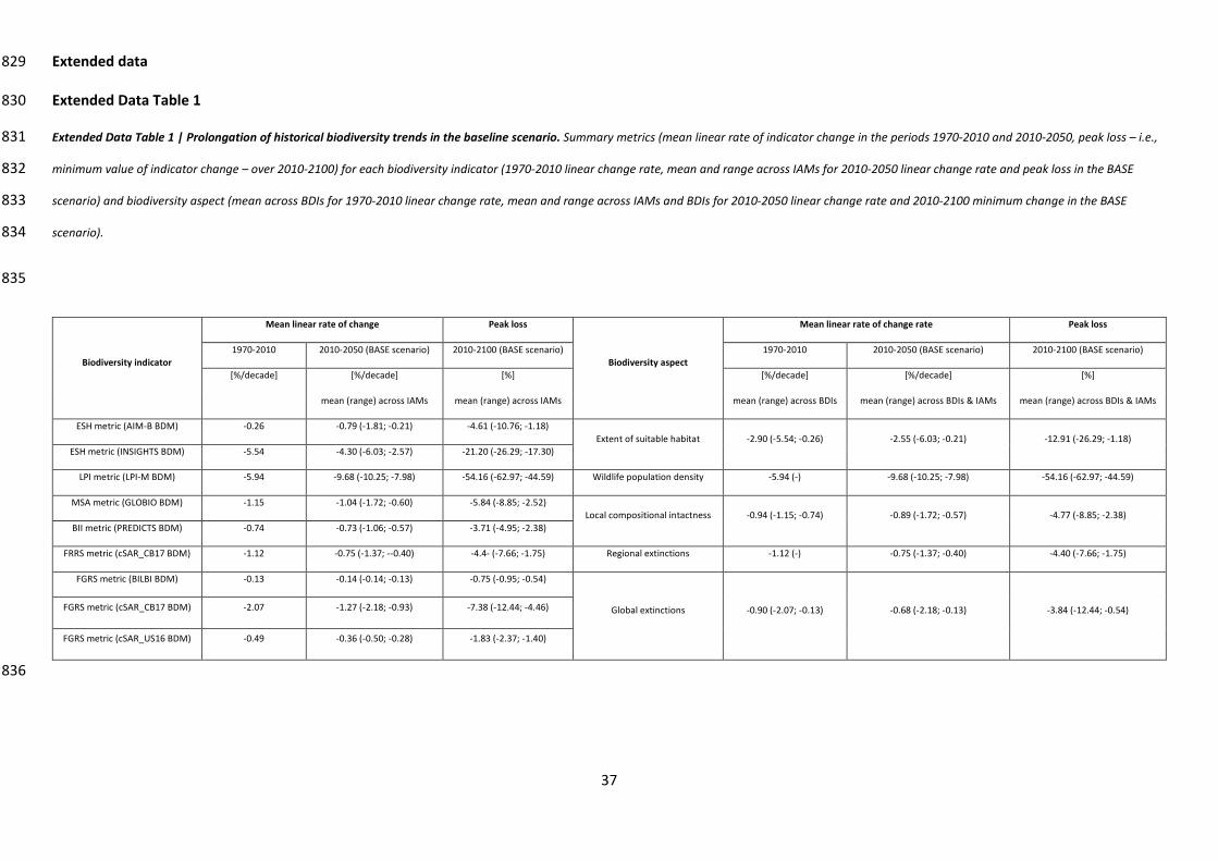
37

Extended data 829

Extended Data Table 1 830

Extended Data Table 1 | Prolongation of historical biodiversity trends in the baseline scenario. Summary metrics (mean linear rate of indicator change in the periods 1970-2010 and 2010-2050, peak loss – i.e., 831

minimum value of indicator change – over 2010-2100) for each biodiversity indicator (1970-2010 linear change rate, mean and range across IAMs for 2010-2050 linear change rate and peak loss in the BASE 832

scenario) and biodiversity aspect (mean across BDIs for 1970-2010 linear change rate, mean and range across IAMs and BDIs for 2010-2050 linear change rate and 2010-2100 minimum change in the BASE 833

scenario). 834

835

Biodiversity indicator

Mean linear rate of change Peak loss

Biodiversity aspect

Mean linear rate of change rate Peak loss

1970-2010 2010-2050 (BASE scenario) 2010-2100 (BASE scenario) 1970-2010 2010-2050 (BASE scenario) 2010-2100 (BASE scenario)

[%/decade] [%/decade] [%] [%/decade] [%/decade] [%]

mean (range) across IAMs mean (range) across IAMs mean (range) across BDIs mean (range) across BDIs & IAMs mean (range) across BDIs & IAMs

ESH metric (AIM-B BDM) -0.26 -0.79 (-1.81; -0.21) -4.61 (-10.76; -1.18) Extent of suitable habitat -2.90 (-5.54; -0.26) -2.55 (-6.03; -0.21) -12.91 (-26.29; -1.18)

ESH metric (INSIGHTS BDM) -5.54 -4.30 (-6.03; -2.57) -21.20 (-26.29; -17.30)

LPI metric (LPI-M BDM) -5.94 -9.68 (-10.25; -7.98) -54.16 (-62.97; -44.59) Wildlife population density -5.94 (-) -9.68 (-10.25; -7.98) -54.16 (-62.97; -44.59)

MSA metric (GLOBIO BDM) -1.15 -1.04 (-1.72; -0.60) -5.84 (-8.85; -2.52) Local compositional intactness -0.94 (-1.15; -0.74) -0.89 (-1.72; -0.57) -4.77 (-8.85; -2.38)

BII metric (PREDICTS BDM) -0.74 -0.73 (-1.06; -0.57) -3.71 (-4.95; -2.38)

FRRS metric (cSAR_CB17 BDM) -1.12 -0.75 (-1.37; --0.40) -4.4- (-7.66; -1.75) Regional extinctions -1.12 (-) -0.75 (-1.37; -0.40) -4.40 (-7.66; -1.75)

FGRS metric (BILBI BDM) -0.13 -0.14 (-0.14; -0.13) -0.75 (-0.95; -0.54)

Global extinctions -0.90 (-2.07; -0.13) -0.68 (-2.18; -0.13) -3.84 (-12.44; -0.54) FGRS metric (cSAR_CB17 BDM) -2.07 -1.27 (-2.18; -0.93) -7.38 (-12.44; -4.46)

FGRS metric (cSAR_US16 BDM) -0.49 -0.36 (-0.50; -0.28) -1.83 (-2.37; -1.40)

836

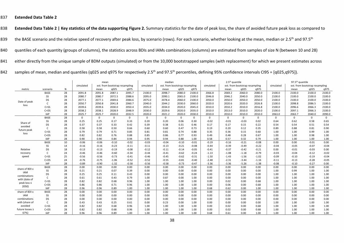
38

Extended Data Table 2 837

Extended Data Table 2 | Key statistics of the data supporting Figure 2. Summary statistics for the date of peak loss, the share of avoided future peak loss as compared to 838

the BASE scenario and the relative speed of recovery after peak loss, by scenario (rows). For each scenario, whether looking at the mean, median or 2.5th and 97.5th 839

quantiles of each quantity (groups of columns), the statistics across BDIs and IAMs combinations (columns) are estimated from samples of size N (between 10 and 28) 840

either directly from the unique sample of BDM outputs (simulated) or from the 10,000 bootstrapped samples (with replacement) for which we present estimates across 841

samples of mean, median and quantiles (q025 and q975 for respectively 2.5th and 97.5th percentiles, defining 95% confidence intervals CI95 = [q025,q975]). 842

mean median 2.5th quantile 97.5th quantile simulated est. from bootstrap resampling simulated est. from bootstrap resampling simulated est. from bootstrap resampling simulated est. from bootstrap resampling

metric scenario N mean q025 q975 mean q025 q975 mean q025 q975 mean q025 q975

Date of peak loss

BASE 28 2091.8 2091.8 2087.1 2095.7 2100.0 2098.7 2080.0 2100.0 2066.8 2069.2 2060.0 2080.0 2100.0 2100.0 2100.0 2100.0 SS 28 2080.7 2080.7 2072.5 2088.6 2095.0 2090.1 2065.0 2100.0 2046.8 2046.2 2040.0 2050.0 2100.0 2100.0 2100.0 2100.0 DS 28 2077.1 2077.1 2069.6 2084.6 2075.0 2078.4 2060.0 2100.0 2050.0 2050.0 2050.0 2050.0 2100.0 2100.0 2100.0 2100.0 C 28 2050.7 2050.8 2041.8 2060.7 2040.0 2044.2 2030.0 2060.0 2020.0 2020.6 2020.0 2026.8 2100.0 2098.8 2086.5 2100.0

C+SS 28 2039.6 2039.6 2030.0 2050.4 2035.0 2034.0 2020.0 2045.0 2010.0 2010.2 2010.0 2016.8 2100.0 2096.6 2066.3 2100.0 C+DS 28 2038.2 2038.1 2028.9 2048.9 2030.0 2029.6 2020.0 2035.0 2010.0 2013.0 2010.0 2020.0 2100.0 2097.1 2066.3 2100.0 IAP 28 2025.7 2025.7 2020.0 2032.5 2020.0 2021.2 2020.0 2030.0 2010.0 2010.0 2010.0 2010.0 2063.0 2063.7 2040.0 2090.0

Share of avoided

future peak loss

BASE 28 0 0 0 0 0 0 0 0 0 0 0 0 0 0 0 0 SS 28 0.25 0.25 0.17 0.33 0.20 0.20 0.06 0.30 -0.02 -0.01 -0.03 0.02 0.64 0.62 0.58 0.65 DS 28 0.37 0.37 0.33 0.42 0.39 0.38 0.31 0.46 0.17 0.17 0.15 0.22 0.54 0.54 0.51 0.54 C 28 0.58 0.58 0.50 0.66 0.60 0.60 0.47 0.73 0.19 0.20 0.12 0.35 0.89 0.88 0.81 0.90

C+SS 28 0.79 0.79 0.71 0.85 0.81 0.81 0.74 0.88 0.35 0.36 0.15 0.60 1.00 1.00 0.99 1.00 C+DS 28 0.82 0.82 0.76 0.88 0.85 0.86 0.77 0.93 0.49 0.48 0.28 0.67 1.00 1.00 0.98 1.00 IAP 28 0.90 0.90 0.84 0.94 0.95 0.94 0.88 1.00 0.58 0.57 0.32 0.79 1.00 1.00 1.00 1.00

Relative recovery

speed

BASE 10 -0.06 -0.06 -0.10 -0.02 -0.03 -0.04 -0.10 -0.01 -0.19 -0.16 -0.21 -0.08 0.00 0.00 -0.01 0.00 SS 14 -0.16 -0.16 -0.23 -0.11 -0.11 -0.13 -0.21 -0.08 -0.44 -0.39 -0.49 -0.22 -0.04 -0.05 -0.07 -0.04 DS 18 -0.13 -0.13 -0.19 -0.08 -0.12 -0.11 -0.14 -0.05 -0.41 -0.37 -0.42 -0.21 0.00 -0.01 -0.03 0.00 C 24 -0.46 -0.46 -0.60 -0.34 -0.44 -0.41 -0.62 -0.24 -1.13 -1.08 -1.18 -0.79 -0.03 -0.04 -0.12 -0.02

C+SS 25 -0.56 -0.56 -0.73 -0.41 -0.46 -0.45 -0.62 -0.31 -1.50 -1.43 -1.56 -1.02 -0.09 -0.10 -0.19 -0.04 C+DS 24 -0.76 -0.75 -1.06 -0.52 -0.52 -0.55 -0.81 -0.40 -2.48 -2.31 -3.44 -1.16 -0.11 -0.13 -0.28 -0.05 IAP 28 -0.89 -0.90 -1.32 -0.58 -0.56 -0.58 -0.73 -0.47 -3.36 -3.36 -5.26 -1.38 -0.08 -0.10 -0.27 0.00

share of BDI x IAM

combinations with (date of peak loss ≤

2050)

BASE 28 0.00 0.00 0.00 0.00 0.00 0.00 0.00 0.00 0.00 0.00 0.00 0.00 0.00 0.00 0.00 0.00 SS 28 0.21 0.21 0.07 0.39 0.00 0.00 0.00 0.00 0.00 0.00 0.00 0.00 1.00 0.99 1.00 1.00 DS 28 0.25 0.25 0.11 0.43 0.00 0.00 0.00 0.00 0.00 0.00 0.00 0.00 1.00 1.00 1.00 1.00 C 28 0.61 0.61 0.43 0.79 1.00 0.87 0.00 1.00 0.00 0.00 0.00 0.00 1.00 1.00 1.00 1.00

C+SS 28 0.82 0.82 0.68 0.96 1.00 1.00 1.00 1.00 0.00 0.02 0.00 0.68 1.00 1.00 1.00 1.00 C+DS 28 0.86 0.86 0.71 0.96 1.00 1.00 1.00 1.00 0.00 0.06 0.00 0.68 1.00 1.00 1.00 1.00 IAP 28 0.96 0.96 0.89 1.00 1.00 1.00 1.00 1.00 0.68 0.62 0.00 1.00 1.00 1.00 1.00 1.00

share of BDI x IAM

combinations with (share of

avoided future losses ≥

67%)

BASE 28 0.00 0.00 0.00 0.00 0.00 0.00 0.00 0.00 0.00 0.00 0.00 0.00 0.00 0.00 0.00 0.00 SS 28 0.00 0.00 0.00 0.00 0.00 0.00 0.00 0.00 0.00 0.00 0.00 0.00 0.00 0.00 0.00 0.00 DS 28 0.00 0.00 0.00 0.00 0.00 0.00 0.00 0.00 0.00 0.00 0.00 0.00 0.00 0.00 0.00 0.00 C 28 0.43 0.43 0.25 0.61 0.00 0.23 0.00 1.00 0.00 0.00 0.00 0.00 1.00 1.00 1.00 1.00

C+SS 28 0.82 0.82 0.68 0.96 1.00 1.00 1.00 1.00 0.00 0.02 0.00 0.68 1.00 1.00 1.00 1.00 C+DS 28 0.82 0.82 0.68 0.96 1.00 1.00 1.00 1.00 0.00 0.02 0.00 0.68 1.00 1.00 1.00 1.00 IAP 28 0.96 0.96 0.89 1.00 1.00 1.00 1.00 1.00 0.68 0.61 0.00 1.00 1.00 1.00 1.00 1.00

39

843 844 845

40

Extended Data Figure 1 846

847

848

Extended Data Fig. 1 | Datasets used to provide spatially explicit input for modeling increased conservation efforts into the land-use models. 849

The figure presents at 30 arcmin-resolution the proportion of land under the assumed expanded protected areas (panel a, based on all areas 850

from the World Database on Protected areas35 and areas from Key Biodiversity Areas36 and Wilderness Areas37) and the value of the assumed 851

spatial priority score for restoration (panel b, Relative Range Rarity-Weighted Species Richness score RRRWSR, based on species range maps 852

from the ICUN Red List41 and the Handbook of the Birds of the World42), as well as the impact of various land uses on the Biodiversity Intactness 853

41

Index (BII38) of various land-use classes (panel c, estimated from assemblage data for 21702 distinct sites worldwide from the PREDICTS 854

database20, 11534 from naturally forested biomes and 10168 from naturally non-forest biomes). Datasets from panels a and c were used to 855

implement spatially explicit restrictions to land-use change within land-use models (from 2020 onwards); datasets from panels b and c were 856

used to implement spatially explicit priorities for restoration and landscape-level conservation planning (from 2020 onwards) in the scenarios 857

were increased conservation efforts are assumed (see Methods). 858

859

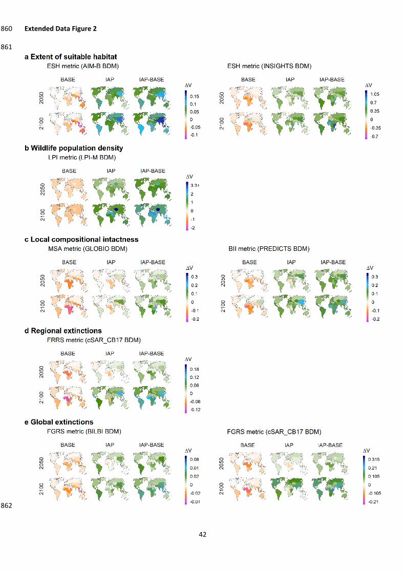
42

Extended Data Figure 2 860

861

862

43

Extended Data Fig. 2 | Spatial patterns in projected changes in the value of biodiversity indicators for BASE and IAP scenarios (and the 863

difference between the IAP and BASE scenarios) for the 17 IPBES subregions, by 2050 and 2100 (as compared to 2010 value). The figure displays 864

the projected changes (mean across IAMs) for each of the eight combinations of biodiversity indicators (BDIs) and biodiversity models (BDMs, 865

see Table 2) for which values at the scale of the IPBES subregions are available, grouped in five aspects of biodiversity (panels a-e). The FGRS 866

indicator was estimated by the cSAR_US16 model only at the global scale.867

44

Extended Data Figure 3 868

869

870

Extended Data Fig. 3 | Projected future global trends in drivers of habitat loss and degradation. Bars indicate for each scenario (colors, mean 871

across all four IAMs) relative change from 2010 to 2050 (upper panel) and 2100 (lower panel) in nine variables (sub-panels). The symbols 872

indicate the IAM-specific values. The variables displayed from the upper left right sub-panel to bottom right sub-panel are: agricultural demand 873

45

for livestock products (Agr. Demand|Liv.), agricultural demand for short-rotation bioenergy crops (Agr. Demand|Crops|Ene.), agricultural 874

demand for crops other than short-rotation bioenergy crops (Agr. Demand|Crops|Non-E.), agricultural supply of livestock products (Agr. 875

Supply|Liv.), agricultural supply of all crop products (Agr. Supply|Crops|Tot.), average yield of crops other than short-rotation bioenergy crops 876

(in metric tonnes dry matter per hectare, Productivity|Crops|Non-E.), and the land dedicated cropland (LC|Cropland) and pasture 877

(LC|Pasture).Values displayed for each variable are change relative to the value of the same variable simulated for 2010, except for two 878

variables (Agr. Demand|Crops|Ene. And Agr. Demand|Crops|Ene.) for which the change in each of these variables is normalized by the sum of 879

values simulated in 2010 for the two variables (i.e., normalization to total demand for crops). 880

46

Extended Data Figure 4 881

882

883 Extended Data Fig. 4 | Projected global trends in land-use change across all scenarios. a) Global trends in the sum of restored land, 884

unmanaged forest and other natural land classes as compared to 2010 (with and without excluding the land abandoned and not yet in 885

restoration – different only for scenarios without increased conservation efforts, see Methods), with thick lines displaying average values across 886

all four IAMs, and ribbons displaying the range across IAMs. Global changes projected in the area of each of the 12 land-use classes (as 887

compared to 2010) for the seven scenarios b) averaged across the four IAMs by 2050 and 2100, and c) for each individual IAM by 2100. 888

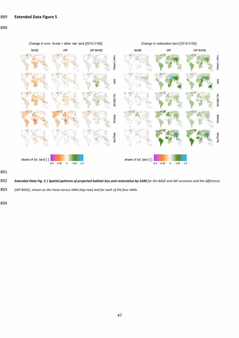
47

Extended Data Figure 5 889

890

891

Extended Data Fig. 5 | Spatial patterns of projected habitat loss and restoration by 2100 for the BASE and IAP scenarios and the difference 892

(IAP-BASE), shown as the mean across IAMs (top row) and for each of the four IAMs. 893

894

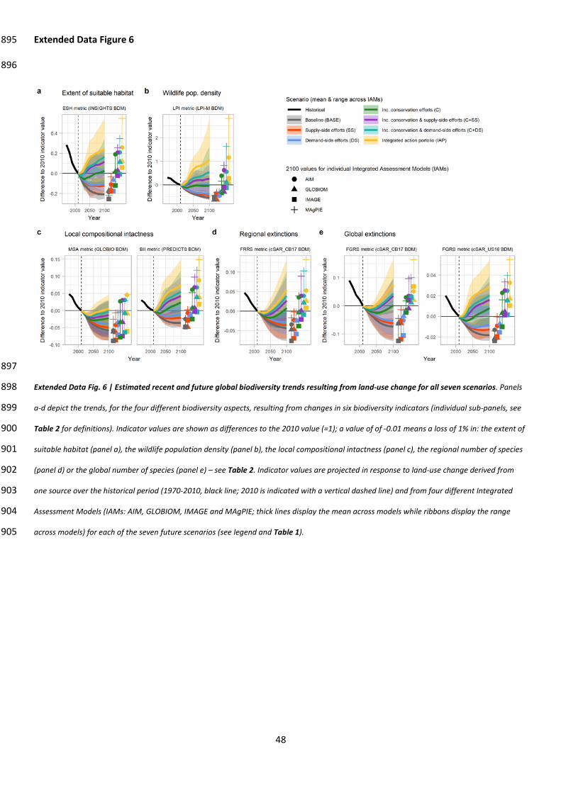
48

Extended Data Figure 6 895

896

897

Extended Data Fig. 6 | Estimated recent and future global biodiversity trends resulting from land-use change for all seven scenarios. Panels 898

a-d depict the trends, for the four different biodiversity aspects, resulting from changes in six biodiversity indicators (individual sub-panels, see 899

Table 2 for definitions). Indicator values are shown as differences to the 2010 value (=1); a value of of -0.01 means a loss of 1% in: the extent of 900

suitable habitat (panel a), the wildlife population density (panel b), the local compositional intactness (panel c), the regional number of species 901

(panel d) or the global number of species (panel e) – see Table 2. Indicator values are projected in response to land-use change derived from 902

one source over the historical period (1970-2010, black line; 2010 is indicated with a vertical dashed line) and from four different Integrated 903

Assessment Models (IAMs: AIM, GLOBIOM, IMAGE and MAgPIE; thick lines display the mean across models while ribbons display the range 904

across models) for each of the seven future scenarios (see legend and Table 1). 905

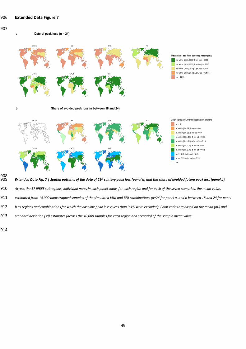
49

Extended Data Figure 7 906

907

908 Extended Data Fig. 7 | Spatial patterns of the date of 21st century peak loss (panel a) and the share of avoided future peak loss (panel b). 909

Across the 17 IPBES subregions, individual maps in each panel show, for each region and for each of the seven scenarios, the mean value, 910

estimated from 10,000 bootstrapped samples of the simulated IAM and BDI combinations (n=24 for panel a, and n between 18 and 24 for panel 911

b as regions and combinations for which the baseline peak loss is less than 0.1% were excluded). Color codes are based on the mean (m.) and 912

standard deviation (sd) estimates (across the 10,000 samples for each region and scenario) of the sample mean value. 913

914

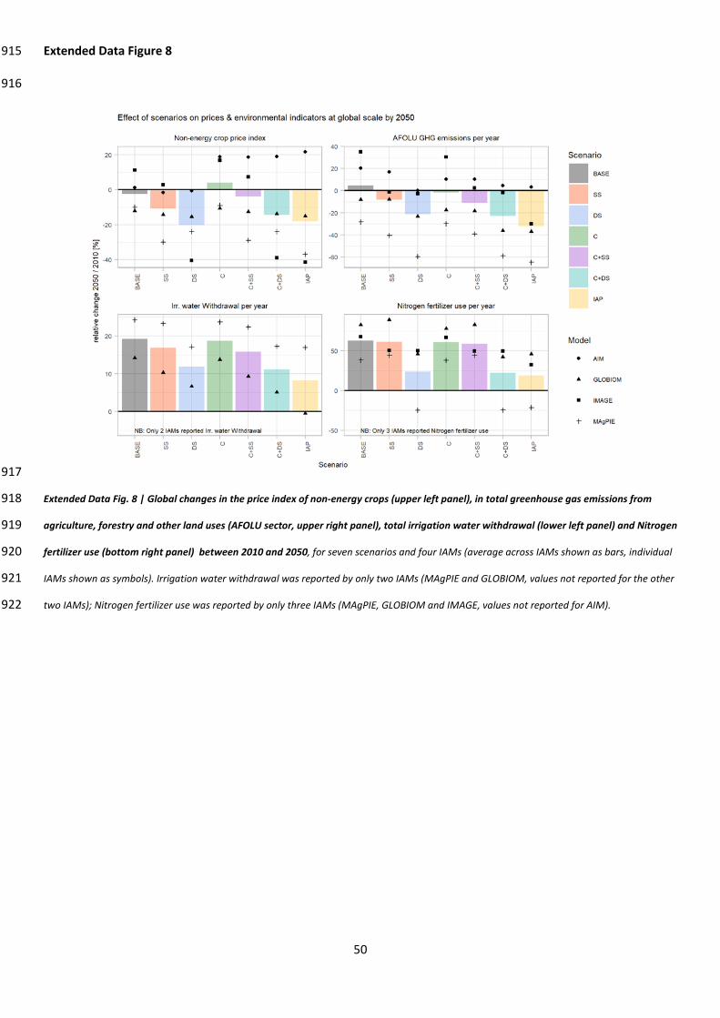
50

Extended Data Figure 8 915

916

917

Extended Data Fig. 8 | Global changes in the price index of non-energy crops (upper left panel), in total greenhouse gas emissions from 918

agriculture, forestry and other land uses (AFOLU sector, upper right panel), total irrigation water withdrawal (lower left panel) and Nitrogen 919

fertilizer use (bottom right panel) between 2010 and 2050, for seven scenarios and four IAMs (average across IAMs shown as bars, individual 920

IAMs shown as symbols). Irrigation water withdrawal was reported by only two IAMs (MAgPIE and GLOBIOM, values not reported for the other 921

two IAMs); Nitrogen fertilizer use was reported by only three IAMs (MAgPIE, GLOBIOM and IMAGE, values not reported for AIM).922

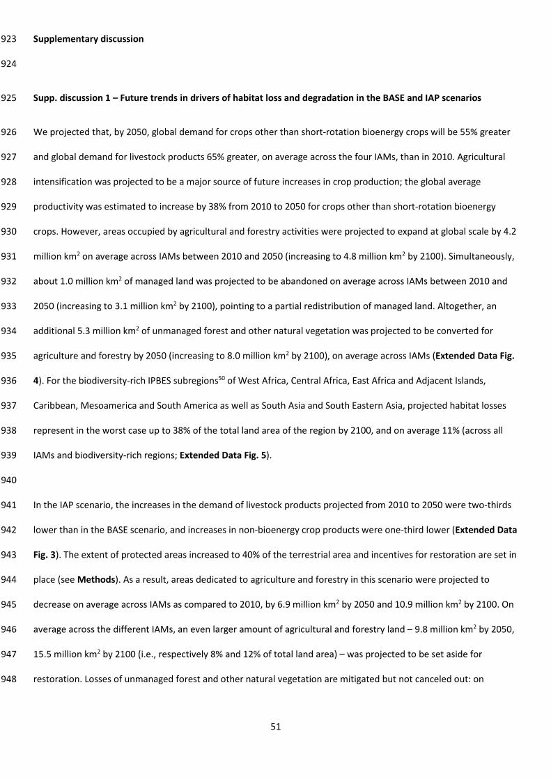
51

Supplementary discussion 923

924

Supp. discussion 1 – Future trends in drivers of habitat loss and degradation in the BASE and IAP scenarios 925

We projected that, by 2050, global demand for crops other than short-rotation bioenergy crops will be 55% greater 926

and global demand for livestock products 65% greater, on average across the four IAMs, than in 2010. Agricultural 927

intensification was projected to be a major source of future increases in crop production; the global average 928

productivity was estimated to increase by 38% from 2010 to 2050 for crops other than short-rotation bioenergy 929

crops. However, areas occupied by agricultural and forestry activities were projected to expand at global scale by 4.2 930

million km2 on average across IAMs between 2010 and 2050 (increasing to 4.8 million km2 by 2100). Simultaneously, 931

about 1.0 million km2 of managed land was projected to be abandoned on average across IAMs between 2010 and 932

2050 (increasing to 3.1 million km2 by 2100), pointing to a partial redistribution of managed land. Altogether, an 933

additional 5.3 million km2 of unmanaged forest and other natural vegetation was projected to be converted for 934

agriculture and forestry by 2050 (increasing to 8.0 million km2 by 2100), on average across IAMs (Extended Data Fig. 935

4). For the biodiversity-rich IPBES subregions50 of West Africa, Central Africa, East Africa and Adjacent Islands, 936

Caribbean, Mesoamerica and South America as well as South Asia and South Eastern Asia, projected habitat losses 937

represent in the worst case up to 38% of the total land area of the region by 2100, and on average 11% (across all 938

IAMs and biodiversity-rich regions; Extended Data Fig. 5). 939

940

In the IAP scenario, the increases in the demand of livestock products projected from 2010 to 2050 were two-thirds 941

lower than in the BASE scenario, and increases in non-bioenergy crop products were one-third lower (Extended Data 942

Fig. 3). The extent of protected areas increased to 40% of the terrestrial area and incentives for restoration are set in 943

place (see Methods). As a result, areas dedicated to agriculture and forestry in this scenario were projected to 944

decrease on average across IAMs as compared to 2010, by 6.9 million km2 by 2050 and 10.9 million km2 by 2100. On 945

average across the different IAMs, an even larger amount of agricultural and forestry land – 9.8 million km2 by 2050, 946

15.5 million km2 by 2100 (i.e., respectively 8% and 12% of total land area) – was projected to be set aside for 947

restoration. Losses of unmanaged forest and other natural vegetation are mitigated but not canceled out: on 948

52

average across IAMs, by 2100 these losses were almost halved in the IAP scenario as compared to the BASE scenario 949

at the global scale (Extended Data Fig. 4-5), and were halved on average in biodiversity-rich regions. 950

951

Supp. discussion 2 – Sources of uncertainties in future projections 952

Using four IAMs made it possible to account explicitly for some of the uncertainty in projected future changes in land 953

use, stemming from differences in model features (such as initial land-use distribution and land-use change 954

dynamics) and from differences in the strategies used to implement the various scenario features in the models. For 955

example, both the residual losses of unmanaged forest and other natural land in biodiversity-rich regions and the 956

increase in restoration land differed significantly between IAMs for the IAP scenario: GLOBIOM and IMAGE projected 957

less optimistic trends than AIM and MAgPIE (Extended Data Fig. 5). The disparity stems from differences between 958

IAMs in the amount of managed grassland that can be restored (lower in GLOBIOM than in other IAMs), the 959

amplitude of preferences towards restoration (lower in IMAGE than in other IAMs) and the amount of deforestation 960

not directly related to the expansion of managed land (higher in IMAGE than in other IAMs). These differences often 961

resulted in greater variation in biodiversity outcome between the IAP and BASE scenarios for AIM and MAgPIE than 962

for the other two IAMs (Fig. 1), and highlight the importance of assessments based on multi-model ensembles, to 963

cover related uncertainties in projected future habitat trends. 964

965

Similarly, using eight BDMs allowed us to account for some uncertainties relating to biodiversity model features 966

(Methods). For example, temporal lags in the response of biodiversity to the restoration of managed land differed 967

between models, often leading to different biodiversity recovery rates within restored land at the global scale for the 968

IAP scenario. Three metrics estimated by three models (ESH metric x AIM-B BDM, FGRS metric x cSAR_US16 BDM 969

and LPI metric x LPI-M BDM) assumed that restored areas are as good as pristine areas for biodiversity, and that the 970

positive impact occurs immediately after shifting to restoration. They therefore provide an upper (optimistic) 971

boundary of biodiversity recovery under restoration. For all other BDIs, restored areas recover to a level of 972

biodiversity that is not always equivalent to that in pristine areas, and for three metrics estimated by two models 973

(MSA x GLOBIO, FRGS x cSAR_CB17 and FRRS x cSAR_CB17), only after several decades. These BDIs provide a more 974

conservative assessment of biodiversity trends – some, such as cSAR_CB17, assumed a linear rate of recovery over 975

53

70 years, which might be viewed as pessimistic. In addition, BDMs estimating the same metric can project different 976

amplitudes of absolute and relative change through time, due to differences in taxonomic coverage, input data and 977

detail in land-use classes. For example, the two BDMs estimating the extent of suitable habitat do so for different 978

sets of taxa and using different land-use classification and input data: AIM-B considers vascular plants, amphibians, 979

reptiles, birds and mammals based on occurrence data, whereas INSIGHTS models only mammals, based on range 980

maps and reported land-use and elevation preferences. Similarly, the difference in the amplitude of projected future 981

relative changes between LPI on the one hand and BII and MSA on the other hand arises from several sources: 982

differences in input data, taxonomic coverage (e.g., birds and mammals for LPI, vs. vertebrates, invertebrates and 983

plants for BII and MSA), whether models rely on observed site- and population-level temporal changes in relative 984

abundance (as for LPI) or on observed differences in sites’ relative abundance (as for BII and MSA), whether they 985

represent the sole impact of land-use change over the entire land area covered by IAMs (as for BII and MSA) or the 986

impacts of both land-use change and other threats (with assumed constant effect across scenarios and time 987

horizons) over a restricted number of grid-cells corresponding to matched sites within the observational record (as 988

for LPI), differences in how species- and site-level data are processed (e.g., truncation to 1 of relative abundances 989

greater than 1 for BII and MSA), and differences in the aggregation of model outputs across grid-cells (e.g., weighting 990

by potential density for BII). Finally, LPI combines species trends using geometric means, which (if declines tend to be 991

concentrated in the less abundant species) has the consequence that LPI declines much more steeply than the 992

average population size; whereas MSA is more directly proportional to average population size, and BII completely 993

so. 994

995

While these differences between models highlight knowledge gaps, all models have different strengths and 996

weaknesses. Using a multi-model ensemble allows us to quantify some of them, thereby allowing more robust 997

conclusions to be reached. This approach is recommended ‘to enable robust decision making and to account for 998

uncertainty in the outcomes of biodiversity models’ by the Intergovernmental Science-Policy Platform on 999

Biodiversity and Ecosystem Services (IPBES 201667, key recommendations of Chapter 4, p122). This approach is also 1000

widely used in other fields, such as climate science14, agrology68, hydrology69 and marine ecosystem modeling70. It 1001

does not account for all types of uncertainties, however. For example, the BDMs implemented in this study, except 1002

for GLOBIO, did not differentiate management practices within cropland, and IAMs did not report this information. 1003

54

Our results may therefore underestimate the future amplitude of both agricultural intensification-driven biodiversity 1004

losses, and biodiversity benefits from agroecological approaches71. Additionally, our approach does not characterize 1005

the uncertainty from individual land-use or biodiversity models, although this can be substantial. For example, in the 1006

context of climate change impact assessment, it has been shown that uncertainties from the parameterization of 1007

individual biodiversity models can be greater than those stemming from using different climate models, and as high 1008

as the uncertainty stemming from which emission scenario is considered72. 1009

1010

Supp. discussion 3 – Feasibility of the various scenarios considered 1011

Our baseline (BASE) scenario relied on the central Middle of the Road SSP2 scenario, which assumes an extension of 1012

historical trends in the future and has been extensively described in the literature16,31,32. We consider this scenario to 1013

be a plausible baseline, and it should not be seen as an overly pessimistic scenario. For example, greater habitat loss 1014

is expected16 for the SSP3 scenario (Regional Rivalry—A Rocky Road), which assumes a human population that 1015

increases continuously over the entire 21st century, a slower increase in crop yields, and setbacks in recent 1016

globalization and land-use regulation trends. 1017

1018

The demand-side and supply-side efforts towards reversing the trends of biodiversity loss were based on options we 1019

consider to be feasible; we excluded assumptions such as increased consumption of artificial meat or insect-based 1020

proteins. Yet, implementing demand-side and supply-side efforts together (IAP scenario) can be viewed as a deep 1021

transformation of anthropogenic use of land, requiring large investments and new policies. For example, the 1022

increases in crop yields we projected in the IAP scenario are, at the global scale, close to estimated recent trends: 1023

depending on the IAM, +34% to +63% between 2010 and 2050, i.e. linear annual rates of increase of between 0.9 1024

and 1.6 percentage points per year (base 2010), compared to estimates over the past 30 years of 0.9 to 1.9 1025

percentage points per year73,74. Yet, this increase implies a doubling of crop yields in Sub-Saharan Africa over the 1026

same period. While significant yield gaps prevailing in this region might offer opportunities75, closing the yield gap in 1027

a sustainable manner will require investments and innovative policies76, and might be complicated by climate 1028

change77. Similarly, halving food waste by 2030 is a Sustainable Development Goal (SDG) target and many action 1029

levers have been identified78. Since we assumed such a target could be achieved by 2050 only, our scenario can be 1030

55

viewed as only moderately ambitious. The proposed efforts will still require country-specific and comprehensive 1031

intervention portfolios, including investment in agricultural and transport infrastructure, training and educational 1032

programs, and improved standards and norms for packaging, storing and recycling. Finally, we assumed a dietary 1033

shift that departs from historical trends and is more ambitious than SSP1 assumptions. However, improving human 1034

health through dietary change is an SDG target, and both evidence and awareness are accumulating that 1035

transitioning towards a ‘flexitarian’ diet could be instrumental in reducing both health and environmental risks25,79. 1036

Evidence of the nature of policy interventions required to trigger dietary transitions is also accumulating80,81, making 1037

our assumption achievable. 1038

1039

Our scenarios aim at biodiversity conservation goals that have already been agreed in principle by Governments3, 1040

but that will require new, ambitious and potentially challenging conservation efforts. Although it seems unlikely that 1041

the globally agreed target of 17% by 2020 will be met6, protected area coverage has increased markedly in recent 1042

decades and there is potential for further increases– some argue that protection of 50% of the Earth’s terrestrial 1043

surface is desirable and achievable82. However, the effectiveness of protected areas is declining, while pressures on 1044

protected areas are growing83. Our assumed increased conservation efforts are ambitious, but rely on a balanced 1045

approach: while we assume an expansion of protected areas to 40% of the terrestrial area with effective 1046

management (i.e., no land-use intensification), >87% of additionally protected areas are identified as wilderness 1047

areas that are by definition under low pressure, and the remaining 3.1% of terrestrial area to be additionally 1048

protected relies solely on priorities that have already been agreed (e.g., Key Biodiversity Areas). Furthermore, in 1049

order to deal with areas that are under pressure (both within and outside protected areas), we rely on landscape-1050

level conservation planning strategies, which seek to increase the restoration of managed areas and to improve the 1051

spatial agency of other land uses84,85. In the IAMs, this is implemented as financial schemes that allow the integration 1052

of spatial preferences for conservation into the land-use decisions pertaining to all terrestrial areas (see Methods). 1053

Financial conservation schemes are increasing in scale and scope, but have been criticized for their poor outcomes 1054

and weak design86. However, such schemes can be improved85, and remain a modeling simplification made for this 1055

analysis; in reality, many other types of tool can be mobilized to achieve landscape-level conservation planning 84,87. 1056

Our scenarios led to the restoration of 4.3-14.6 million km2 (i.e., 3-11% of terrestrial area) by 2050, which might be 1057

compatible with currently agreed targets and momentum towards restoration (e.g., Bonn Challenge, UNCCD’s Land 1058

56

Degradation Neutrality target-setting program). In the models, these efforts are assumed to have already partially 1059

started in 2020 in the most ambitious scenarios. In addition, our baseline scenario is based on SSP2, in which land-1060

use trajectories and conservation efforts differ across models but are not aimed at accurately representing the 1061

observed land-use change and conservation efforts until 2020. This implies that differences in model projections 1062

between scenarios by 2020 and 2030 cannot be used to diagnose the impact of various assumptions about 1063

additional actions over this period in the real world. 1064

1065

The equity of proposed actions should be considered when assessing their feasibility. Solutions that transfer future 1066

development opportunities from biodiversity-rich regions to high-yielding and less biodiversity-rich regions, as well 1067

as foregone opportunities for producers in large production regions as a result of demand-side efforts, might not be 1068

perceived as acceptable or fair. In our view, such issues are inevitably associated with deep transformations of our 1069

land-use system, and require a more comprehensive analysis, including options of intra- and inter-national social 1070

transfers. However, we tried to avoid unnecessarily unfair solutions in two ways. First, our modeling relied partly on 1071

market-like dynamics (rather than solely on restrictive assumptions) to resolve the trade-offs arising from a 1072

progressive shift in societal preferences from production to conservation land use. Future habitat conversion in all 1073

regions was not strictly forbidden, but was made progressively less desirable through economic incentives. The 1074

expanded protected areas (where conversion was strictly forbidden) were mostly located in low-yielding and less 1075

biodiversity rich regions (see Extended Data Fig. 1). This left ample room for habitat conversion and exploitation of 1076

economic opportunities in biodiversity-rich regions, where projected conversion was only halved in the IAP scenario 1077

as compared to the BASE scenario (see Extended Data Fig. 5). Second, the biodiversity score used to inform the 1078

spatial priorities that minimize the biodiversity impacts of future land-use conversions (see Methods) was based on a 1079

regional relative range-rarity score, rather than a global absolute range-rarity score. This implies prioritizing spatial 1080

configurations within regions, while avoiding prioritizing one region over another based on their absolute levels of 1081

biodiversity, although this might be justified based solely on biodiversity considerations. 1082

1083

1084

1085

57

Supp. discussion 4 – Mapping of scenarios to the Sustainable Development Goals (SDGs) 1086

Our analysis focuses on the trade-off between food provision and conservation, and we did not seek to quantify the 1087

extent to which our IAP scenario contributes towards achieving the broader Sustainable Development Goals (SDGs). 1088

However, our scenarios can be positioned with respect to the SDGs as evidence suggests that actions depicted in our 1089

IAP scenario could contribute significantly towards several SDGs and help reduce the food production system’s 1090

pressure on planetary boundaries25,88. SSP2 – defining our baseline scenario – pictures a future in which the 1091

development of economic growth and inequalities, together with land-use developments, lead to reduced food 1092

insecurity89 and poverty90, therefore contributing towards SDGs 1 (No poverty), 2 (Zero hunger) and SDG 10 1093

(Reduced inequalities). Our BASE scenario fully reflects related land-use developments, while our IAP scenario may 1094

achieve better outcomes for SDG2. While dietary preferences follow historical trends in the BASE scenario, the 1095

dietary shift assumed as part of demand-side efforts could allow significant progress towards SDGs 3 (Good health 1096

and well-being) and 13 (Climate action). Halving waste throughout the supply chain is an explicit target of SDG 12 1097

(Responsible consumption and production), while the reductions in agricultural water withdrawal in the IAP scenario 1098

would facilitate achieving SDG 6 (Clean water and sanitation) and make a significant contribution to SDG 14 (Life 1099

below water). Improved conservation efforts would make a significant contribution towards SDG 15 (Life on land). 1100

1101

Supp. discussion 5 – Other biodiversity aspects and threats 1102

Terrestrial biodiversity is a multifaceted concept, encompassing different aspects at various geographical and time 1103

scales, including the local diversity, abundance and uniqueness of genes, species, populations, traits and functions of 1104

living organisms across multiple taxonomic groups, as well as their variation across landscapes and biomes, and their 1105

genetic and ecological history. The models used in our study cover a broader range of biodiversity aspects and 1106

taxonomic groups than those in many previous studies 91,92, but they do not provide estimates of trends in some 1107

biodiversity aspects such as phylogenetic diversity and functional diversity – key indicators of the long-term ability of 1108

ecosystems to cope with future changes. 1109

1110

While it cannot be ensured that trends in these unmodelled terrestrial biodiversity aspects would be reversed in our 1111

most ambitious scenario, we can clarify the anticipated implications of our results for these biodiversity aspects. For 1112

58

example, it has been shown for mammals that conserving functional and phylogenetic diversity on top of taxonomic 1113

diversity might require a substantially larger amount of protected area93. This suggests that our results may be 1114

optimistic if extended to terrestrial biodiversity in general; greater effort may be required to ensure a reversal of 1115

trends across additional aspects of biodiversity. However, priorities may not be simply cumulative, and there may be 1116

overlap and synergies between strategies to conserve multiple aspects of biodiversity94. In our study, the assumed 1117

increased conservation efforts were already designed to balance different conservation priorities: for example, the 1118

restoration priority score (based on relative range rarity) incorporates both local richness and endemism. In addition, 1119

the expanded protected areas encompass identified biodiversity hotspots (e.g., current WDPAs and KBAs) but also 1120

intact ecosystems, expected to host high levels of functional diversity95. In addition, the level of ambition in our 1121

increased conservation effort scenarios is high: an addition of 25% of land to the 15% already protected (resulting in 1122

40% of land protected) while spatial synergies between strategies to conserve multiple aspects of biodiversity were 1123

already found when investigating a smaller addition of 15% of land94. Overall, we believe that our scenarios may 1124

have the ambition needed to reverse additional terrestrial biodiversity aspects (as affected by land-use change), 1125

although tackling additional aspects may require adjustments in spatial priorities. 1126

1127

We account only for the effects on biodiversity of habitat loss due to land-use change, but in reality, biodiversity 1128

faces multiple threats. According to IUCN Red List data, the expansion and intensification of agriculture is imperiling 1129

5,407 species (62% of species listed as threatened or near-threatened), but half as many species (2,700) are 1130

adversely affected by hunting or fishing, 2,298 species are adversely affected by biological invasions and diseases, 1131

and 1,688 by climate change5. Land-use change is currently the largest single threat to biodiversity5, but other 1132

threats will increase in importance in the future, in particular climate change96,97. Our scenarios are focused on the 1133

largest threat, so our most ambitious scenario provides a strong indication of the actions required, but as threats 1134

intensify and shift, these actions may not be sufficient to reverse terrestrial biodiversity trends fully. This reinforces 1135

that integrated strategies, in combination with bold targets, must be central to the post-2020 biodiversity strategy. 1136

59

Supplementary discussion additional references 1137

67. IPBES. The methodological assessment report on scenarios and models of biodiversity and ecosystem 1138

services. (2016). 1139

68. Martre, P. et al. Multimodel ensembles of wheat growth: Many models are better than one. Glob. Chang. 1140

Biol. 21, 911–925 (2015). 1141

69. Schewe, J. et al. Multimodel assessment of water scarcity under climate change. Proc. Natl. Acad. Sci. U. S. A. 1142

111, 3245–50 (2014). 1143

70. Meier, H. E. M. et al. Comparing reconstructed past variations and future projections of the Baltic Sea 1144

ecosystem - First results from multi-model ensemble simulations. Environ. Res. Lett. 7, (2012). 1145

71. Balmford, A. et al. The environmental costs and benefits of high-yield farming. Nat. Sustain. 1, 477–485 1146

(2018). 1147

72. Thuiller, W., Guéguen, M., Renaud, J., Karger, D. N. & Zimmermann, N. E. Uncertainty in ensembles of global 1148

biodiversity scenarios. Nat. Commun. 10, 1–9 (2019). 1149

73. Iizumi, T. et al. Uncertainties of potentials and recent changes in global yields of major crops resulting from 1150

census- and satellite-based yield datasets at multiple resolutions. PLoS One 13, e0203809 (2018). 1151

74. Ray, D. K., Ramankutty, N., Mueller, N. D., West, P. C. & Foley, J. a. Recent patterns of crop yield growth and 1152

stagnation. Nat. Commun. 3, 1293 (2012). 1153

75. Mueller, N. D. et al. Closing yield gaps through nutrient and water management. Nature 490, 254–7 (2012). 1154

76. Garnett, T. et al. Sustainable Intensification in Agriculture: Premises and Policies. Science (80-. ). 341, 33–4 1155

(2013). 1156

77. Rosenzweig, C. et al. Assessing agricultural risks of climate change in the 21st century in a global gridded crop 1157

model intercomparison. Proc. Natl. Acad. Sci. 1–6 (2013). doi:10.1073/pnas.1222463110 1158

78. Parfitt, J., Barthel, M. & MacNaughton, S. Food waste within food supply chains: Quantification and potential 1159

for change to 2050. Philos. Trans. R. Soc. B Biol. Sci. 365, 3065–3081 (2010). 1160

79. Bajželj, B. et al. Importance of food-demand management for climate mitigation. Nat. Clim. Chang. 4, 924–1161

929 (2014). 1162

80. Mozaffarian, D. Dietary and Policy Priorities for Cardiovascular Disease, Diabetes, and Obesity. Circulation 1163

133, 187–225 (2016). 1164

60

81. Hyseni, L. et al. The effects of policy actions to improve population dietary patterns and prevent diet-related 1165

non-communicable diseases: Scoping review. Eur. J. Clin. Nutr. 71, 694–711 (2017). 1166

82. Dinerstein, E. et al. An Ecoregion-Based Approach to Protecting Half the Terrestrial Realm. Bioscience 67, 1167

534–545 (2017). 1168

83. Watson, J. E. M., Dudley, N., Segan, D. B. & Hockings, M. The performance and potential of protected areas. 1169

Nature 515, 67–73 (2014). 1170

84. Sayer, J. et al. Ten principles for a landscape approach to reconciling agriculture, conservation, and other 1171

competing land uses. Proc. Natl. Acad. Sci. U. S. A. 110, 8349–56 (2013). 1172

85. McDonald, J. A. et al. Improving private land conservation with outcome-based biodiversity payments. J. Appl. 1173

Ecol. 55, 1476–1485 (2018). 1174

86. Ferraro, P. J. & Pattanayak, S. K. Money for Nothing? A Call for Empirical Evaluation of Biodiversity 1175

Conservation Investments. PLoS Biol. 4, e105 (2006). 1176

87. Dudley, N. et al. The essential role of other effective area-based conservation measures in achieving big bold 1177

conservation targets. Glob. Ecol. Conserv. 15, 1–7 (2018). 1178

88. Obersteiner, M. et al. Assessing the land resource-food price nexus of the Sustainable Development Goals. 1179

Sci. Adv. 2, e1501499–e1501499 (2016). 1180

89. Hasegawa, T., Fujimori, S., Takahashi, K. & Masui, T. Scenarios for the risk of hunger in the twenty- first 1181

century using Shared Socioeconomic Pathways. Environ. Res. Lett. 10, (2015). 1182

90. Byers, E. et al. Global exposure and vulnerability to multi-sector development and climate change hotspots. 1183

Environ. Res. Lett. 13, 055012 (2018). 1184

91. Nicholson, E. et al. Scenarios and Models to Support Global Conservation Targets. Trends Ecol. Evol. 34, 57–68 1185

(2019). 1186

92. Pereira, H. M. et al. Scenarios for global biodiversity in the 21st century. Science (80-. ). 330, 1496–1501 1187

(2010). 1188

93. Brum, F. T. et al. Global priorities for conservation across multiple dimensions of mammalian diversity. Proc. 1189

Natl. Acad. Sci. 114, 7641–7646 (2017). 1190

94. Pollock, L. J., Thuiller, W. & Jetz, W. Large conservation gains possible for global biodiversity facets. Nature 1191

546, 141–144 (2017). 1192

61

95. Watson, J. E. M. et al. The exceptional value of intact forest ecosystems. Nat. Ecol. Evol. in press, (2018). 1193

96. Newbold, T. Future effects of climate and land-use change on terrestrial vertebrate community diversity 1194

under different scenarios. Proc. R. Soc. B Biol. Sci. 285, 20180792 (2018). 1195

97. Pacifici, M. et al. Species’ traits influenced their response to recent climate change. Nat. Clim. Chang. 7, 205–1196

208 (2017). 1197

1198

62

1199