Tissue-mimicking agar gelatin materials for use in ... · Tissue-mimicking materials for elastography 5599 Long-term stability of lesion diameters and T 2 relaxation times in the

INSTITUTE OF PHYSICS PUBLISHING PHYSICS IN MEDICINE AND BIOLOGY

Phys. Med. Biol. 50 (2005) 5597–5618 doi:10.1088/0031-9155/50/23/013

Tissue-mimicking agar/gelatin materials for use inheterogeneous elastography phantoms

Ernest L Madsen, Maritza A Hobson, Hairong Shi, Tomy Vargheseand Gary R Frank

Department of Medical Physics, University of Wisconsin, 1300 University Avenue, Room 1530,Madison, WI 53706, USA

E-mail: [email protected]

Received 3 May 2005, in final form 24 August 2005Published 16 November 2005Online at stacks.iop.org/PMB/50/5597

AbstractFive 9 cm × 9 cm × 9 cm phantoms, each with a 2-cm-diameter cylindricalinclusion, were produced with various dry-weight concentrations of agar andgelatin. Elastic contrasts ranged from 1.5 to 4.6, and values of the storagemodulus (real part of the complex Young’s modulus) were all in the soft tissuerange. Additives assured immunity from bacterial invasion and can producetissue-mimicking ultrasound and NMR properties. Monitoring of strain ratiosover a 7 to 10 month period indicated that the mechanical properties of thephantoms were stable, allowing about 1 month for the phantom to reachchemical equilibrium. The only dependable method for determining the storagemoduli of the inclusions is to make measurements on samples excised from thephantoms. If it is desired to produce and accurately characterize a phantomwith small inclusions with other shapes, such as an array of small spheres,an auxiliary phantom with the geometry of the cylindrical inclusion phantomsor the equivalent should be made at the same time using the same materials.The elastic contrast can then be determined using samples excised from theauxiliary phantom. A small increase of about 10% in volume of the cylindricalinclusions occurred—a tolerable increase. Interestingly, the smallest increase(about 5%) occurred in the phantom with the largest elastic contrast.

1. Introduction

Phantoms for use in elastography have been produced in many laboratories over the last decade.Usually the phantoms produced are ad hoc, and there is little concern for long-term stabilityof physical properties or for immunity from deterioration due to environmental variations(e.g. temperature). Also, although values of elasticity properties of materials are reported,little attention has been given to the degree to which elastography phantom materials also

0031-9155/05/235597+22$30.00 © 2005 IOP Publishing Ltd Printed in the UK 5597

http://dx.doi.org/10.1088/0031-9155/50/23/013

mailto:[email protected]

http://stacks.iop.org/PMB/50/5597

5598 E L Madsen et al

possess tissue-mimicking (TM) values of ultrasound and/or NMR properties. For example,if the ultrasound attenuation coefficient is a reasonable approximation for a target tissue, butthe propagation speed is 900 m s−1 instead of the 1540 m s−1 assumed by the scanner, thenelastographic performance might appear to be acceptable to 15 cm depth at a nominal 7 MHzscanner frequency instead of to a depth of 15 cm × 900/1540 ≈ 9 cm. A thorough reviewof the literature on elastography phantoms has been included in a recent publication (Madsenet al 2003); thus, a review of only published work most closely related to that reported in thispaper is given here.

Mixtures of agar and gelatin were used in phantoms for use in elastography by de Korteet al (1997). Three homogeneous samples were made with 1%, 2% and 3% dry-weight agar,the dry-weight concentration of gelatin being 8% in all three. The samples were congealedby immersing in ice water, and no cross-linking agent was employed to elevate the meltingpoint of the final materials above that of gelatin; the melting point of typical gelatins is about32 ◦C. The ‘compressibility modulus’ was monitored for a 4 h period following congealing;there was no long-term stability study done.

Other investigators have produced heterogeneous phantoms using agar/gelatin mixtures(Kallel et al 2001). The dry-weight gelatin concentration was different in the backgroundmaterials than in the inclusions, and as a result of osmosis the diameters of the inclusionschanged considerably over a period of 2 weeks. Similar phantoms, in which variations in thedry-weight concentration of gelatin were employed to cause elastic contrast, were producedby Gao et al (1995). As in the case of the phantoms made by Kallel et al (2001), osmosis dueto differences in dry-weight gelatin concentrations would preclude long-term stability.

It has been observed in our laboratory that an aqueous agar background does not changesize or shape significantly even though the dry-weight agar concentration of the inclusionmaterial differs from that of its surroundings. This geometric stability does not exist forgelatin inclusions in gelatin surroundings, i.e., if the initial dry-weight gelatin concentrationin the inclusion is greater than or less than that in the surroundings, the inclusion will increaseor decrease in volume, respectively, presumably due to osmosis. Thus, for an aqueous mixtureof agar and gelatin, a reasonable expectation is that the shape and size of inclusions willnot change if the dry-weight gelatin concentration is the same in the inclusions as in thesurroundings, while the dry-weight agar concentration in inclusions can be different than inthe surroundings. When the dry-weight gelatin concentration is different in the inclusionsthan in the surroundings—as in the case of Kallel et al (2001)—it is reasonable that the sizeof an inclusion would change with time due to osmosis.

Before the advent of elastography, Madsen et al (1991) reported a low MR contrastspherical lesion phantom for use in MRI where the dry-weight gelatin concentration wasuniform throughout, but the dry-weight agar concentration was 2.7% in the backgroundand lower in the spheres. The lower agar concentration produced higher values of thelongitudinal relaxation time (T1) and the transverse relaxation time (T2) in the spheres than inthe background resulting in clinically relevant MR (object) contrast. (Object contrast dependson bulk material parameters; thus, in this case the ratio of T2 for the sphere material dividedby the T2 for the background material might be considered the T2 object contrast.) Thedry-weight agar concentration in one set of spheres was 1.35% and in another set of sphereswas 2.02%; thus, the object contrast in the former case (1.35% agar) was greater than in thelatter case (2.02% agar). Each set contained spheres ranging in diameter from 2 mm through9.5 mm; thus, the test for the MRI unit was to determine the smallest sphere diameter of eachcontrast; the phantom might be referred to as a spherical lesion ‘contrast-detail’ phantom. Thephantom also contained formaldehyde throughout to cross-link the gelatin, raising the meltingpoint to 78 ◦C where the agar component melts.

Tissue-mimicking materials for elastography 5599

Long-term stability of lesion diameters and T2 relaxation times in the ‘contrast-detail’phantom was assessed with two auxiliary phantoms made specifically for testing long-termstability of those parameters. One phantom contained two 3.18-cm-diameter spheres, one ofeach object contrast found in the ‘contrast-detail’ phantom. The second phantom was identicalexcept that the two spheres were 0.95 cm in diameter. The larger diameters allowed T2s inthe spheres and in the background to be measured directly in the phantom with a GE Signaclinical MR unit. Three glass bottles, each containing one of the three types of material,were produced at the time the auxiliary phantoms were made, using the same materials. T2swere measured in these three uniform materials at the same time T2s were measured in thetwo auxiliary phantoms. Thus, any drift in T2 values due to the direct contact of differentmaterials in the auxiliary phantoms could be monitored. The diameters of the spheres werealso monitored by making MR images with the scan planes through the centres of the spheres.T2s in the auxiliary phantoms and in the corresponding uniform materials in the glass bottlesremained within a few per cent of one another over the times monitored (14 weeks in the caseof the 3.18-cm sphere phantom and 20 months in the case of the 0.95-cm sphere phantom).Also, over the periods monitored the diameters of the spheres on MR images did not changeperceptibly, indicating long-term stability of geometry.

As in the Madsen et al case, Plewes et al (2000) produced an agar/gelatin phantom inwhich the agar concentration was different in the inclusion than in the background, whilethe gelatin concentration was the same throughout the phantom. Thus, the size and shape ofthe inclusion would likely have been temporally stable. However, neither elastic nor NMRproperties were monitored over time to assess long-term stability, and apparently there was nocross-linking agent used to raise the melting point above that of the gelatin per se. (Withoutcross-linking our gelatin melts at 32 ◦C.)

Since higher agar concentrations produce noticeably stiffer materials, it is reasonableto expect that higher agar concentrations in agar/gelatin materials will correspond to higherYoung’s moduli. In this paper, we report on the long-term stability of inclusion geometries andon the stability of Young’s moduli and elastic contrasts for heterogeneous phantoms in whichthe gelatin concentration is constant throughout the agar/gelatin mixtures in each phantom,while the agar concentration differs between inclusion and background. The phantoms consistof 9 cm × 9 cm × 9 cm cubes of background material with 2-cm-diameter cylindricalinclusions. The materials have NMR relaxation times, T1 and T2, which mimic soft tissues.Without appropriate additives, the ultrasound propagation speeds and attenuation coefficientsare lower than those typical for soft tissues, and NMR T1s are higher than those in most softtissues. Values of propagation speeds can easily be elevated with addition of solutes and tissue-mimicking values of attenuation coefficients can be produced with addition of microscopicparticulates. The latter solutes and particulates can be chosen to affect the NMR relaxationtimes negligibly. Independently, NMR T1s can be lowered with addition of a Cu2+ salt plusEDTA (ethylene diamine tetraacetic acid), the latter to assure long-term stability (Rice et al1998).

Extensive testing of the long-term stability of inclusion geometries and elastic propertiesof component materials is reported for a set of five heterogeneous agar/gelatin phantoms.

2. Materials and production methods

Each agar/gelatin component in the phantom contains (dissolved) granulated agar (FisherScientific, Pittsburgh, PA, cat. no. BP1423), ‘200 bloom’ gelatin derived from calf skin(Vyse Gelatin Company, Schiller Park, IL), 18 M� cm deionized water, CuCl2-2H2O,EDTA-tetra Na hydrate [ethylenediaminetetraacetic acid tetrasodium hydrate] (Aldrich,


Milwaukee, WI, cat. no. E2,629–0), NaCl, an antibacterial agent (as described in detaillater) and HCHO (formaldehyde). The gelatin likely is responsible for the bonding thatforms between inclusions and background materials. Increased dry-weight concentration ofagar produces greater stiffness (higher Young’s modulus). EDTA forms a chelate with theCu2+ ions, sufficient EDTA being present that all Cu2+ ions are attached to EDTA. Thepurpose of forming the chelate is to allow the Cu2+ to remain mobile, thus allowing controlledlowering of the T1 relaxation time. (Without EDTA, the Cu2+ ions slowly become immobilizedby attaching to the gelatin molecules, thus eliminating their T1-lowering capacity.) NaCl ispresent in sufficient concentration to produce tissue-like NMR coil loading. Formaldehydecross-links gelatin molecules raising the melting point of the material to over 65 ◦C. In onephantom, prevention of fungal and bacterial invasion was accomplished with 1.0 g l−1 ofthimerosal, a mercury-containing compound used in earlier elastography phantoms (Madsenet al 2003); in the other phantoms prevention was done with a less toxic preservative calledGermall-plus R© (International Specialty products, Wayne, NJ, USA) which contains no mercuryand is therefore environmentally more acceptable. Also, some phantoms contain rather highconcentrations of microscopic glass beads to increase ultrasonic attenuation and backscatterto tissue-like levels.

For the five heterogeneous phantoms reported in this paper (referred to as phantoms A, B,C, D and E), the concentrations of the various components differ from one phantom to another;however, within any one phantom the dry-weight gelatin concentration is constant throughout,stiffness differences resulting primarily from differences in dry-weight agar concentrations.

The procedure for making the agar/gelatin materials is presented in the form of anexample; namely, the production of 1.2 l of the background material in phantom B. Otheragar/gelatin materials are made in the same way with differences in concentrations of oneor more components. First, quantities of molten gelatin and molten agar are made. Usingdifferent beakers, 50.4 g of dry gelatin and 64.5 g of glass beads (Potters Industries, Parsippany,NJ, USA; catalog number 4000E) are added to 460 cc of 18 M� cm room-temperature distilledwater, and 16.33 g of dry agar are added to 800 cc of 18 M� cm room-temperature distilledwater. The two mixtures are heated in double boilers; thus, the beakers are not in directcontact with the heat sources to avoid overheating at the bottoms of the beakers. After the twomaterials have clarified (Usually clarification has occurred when the temperature has risen tothe 90 ◦C range.), 460 cc of the molten gelatin and 720 cc of the molten agar are mixed togetherin another beaker. (The volume per cents are approximately 40% and 60%, respectively, for allagar/gelatin materials reported here.) While the mixture is at 70–80 ◦C, 4.1 g of EDTA-tetraNa hydrate is completely dissolved into it. Then 1.4 g of CuCl2-2H2O and 9.6 g of NaClare dissolved. By partially immersing the beaker in cold water and stirring, the mixture iscooled to 50 ◦C, and 18 g of Germall-plus are dissolved into it. The mixture is then cooledto 36 ◦C and 3.0 cc of formalin solution is mixed in. (Note that formalin solution is 37%formaldehyde.) At this point, the molten agar/gelatin is ready to be poured into a mould forcooling and congealing overnight to room temperature.

The glass beads present in the materials contribute to both scattering and attenuation.The 4000E beads have the following typical diameter distribution: 10% are less than 5 µm,50% are less than 18 µm and 90% are less than 45 µm. The mean diameter of these beads istypically 20 µm.

2.1. Heterogeneous phantoms

Each phantom produced consists of a 9 cm × 9 cm × 9 cm cube of background materialwith a 2-cm-diameter cylindrical inclusion which is perpendicular to two sides. A diagram


(a) (b)

Figure 1. Heterogeneous phantom geometry used in long-term stability tests: (a) view with theaxis of the cylindrical inclusion perpendicular to the figure; (b) view with the axis parallel to theplane of the figure.

Table 1. Dry-weight per cents of the various components in the phantoms. The weight per centof 18 M� cm water is not shown since it just makes up the remainder. The gelatin concentrationsin the background and inclusion of any one phantom are the same in the agar/gelatin when glassbeads are excluded; because of the significant difference in glass bead concentrations betweenbackground and inclusions in phantoms D and E, the weight-per cent of gelatin, e.g., gelatin ishigher in the inclusion than in the background.

CuCl2- EDTA tetra- Germall Glass beadMaterial Agar Gelatin 2H2O Na hydrate NaCl HCHO plus scatterers

Phantom A background 1.17 3.60 0.113 0.33 0.77 0.24 – 4.6Phantom A inclusion 3.53 3.60 0.113 0.33 0.77 0.24 1.45 5.6Phantom B background 1.17 3.60 0.113 0.33 0.77 0.24 1.45 4.6Phantom B inclusion 3.53 3.60 0.113 0.33 0.77 0.24 1.45 5.6Phantom C background 1.17 5.52 0.113 0.33 0.77 0.24 1.45 4.4Phantom C inclusion 3.53 5.52 0.113 0.33 0.77 0.24 1.45 5.4Phantom D background 1.17 5.52 0.113 0.33 0.77 0.24 1.45 4.4Phantom D inclusion 3.64 5.70 0.116 0.34 0.80 0.25 1.50 0.0Phantom E background 1.11 4.80 0.114 0.33 0.77 0.32 1.45 3.4Phantom E inclusion 3.44 4.92 0.116 0.34 0.79 0.33 1.49 0.75

is shown in figure 1. The cylinder is centred in the phantom, i.e., the axis of the cylinder is4.5 cm from four surfaces of the cubic phantom. The dry-weight gelatin concentration isconstant throughout each phantom, including background and inclusion. The concentrationfor each component in the phantoms is shown in table 1.

Each phantom is produced in two basic steps. First, the background is made. The mouldto receive the molten background material is an acrylic box open at opposite ends over whichSaran Wrap is epoxied. The barrel of a sawed-off 30 cc hypodermic syringe is epoxied intoa hole in one acrylic wall near one corner of the box. An acrylic cylindrical rod passesthrough holes in opposite sides of the box. ‘Five-minute’ epoxy (3M Scotch Weld DP100,3M Industrial Adhesives and Tapes, St. Paul, MN, USA) ensures a seal between the rod andthe holes in the box. This epoxy forms an adequate bond with acrylic but can be removedrather easily with a knife. Prior to gluing on the last Saran Wrap layer, all surfaces which willbe in contact with the molten background material are coated with a thin layer of petrolatum.


This layer allows clean removal of the stainless steel rods and then removal of the completedbackground from the mould.

After the 40 ◦C molten background material has been introduced into the mould andsyringe barrel through the projecting syringe barrel, the syringe piston is inserted into thesyringe barrel and rubber bands attached to maintain positive gauge pressure on the material asit congeals. Note that before the molten background material is poured in, acrylic constrainingplates are taped over the Saran Wrap sides to assure flatness of those sides of the backgroundmaterial. The entire apparatus is mounted on a rotator so that rotation at 2 rpm about ahorizontal axis occurs throughout the congealing period; thus, gravitational sedimentation ofglass beads, etc, is avoided.

After about 24 h, formaldehyde cross-linking will have raised the melting point of thematerial above 60 ◦C. Then the second production step is carried out, namely, production ofthe inclusion. The epoxy seals around the acrylic rod are removed and the rod is withdrawn.The hole in the gel is then quickly and gently cleaned with Kimwipes R© (Kimberly-ClarkCorporation, Roswell, Georgia, USA) soaked in detergent solution and rinsed with 18 M� cmwater. Tape is applied over one opening in the acrylic wall and 40 ◦C molten inclusionmaterial is poured into the remaining opening filling the hole. Since the background is at roomtemperature, the inclusion material congeals within minutes.

After another 24 h to allow formaldehyde cross-linking of the inclusion material, a knifeedge is used to cut the cylindrical inclusion flush with the sides of the phantom, and thephantom is removed from the acrylic-and-Saran-Wrap mould and submersed in safflower oilin a plastic container. The container is sealed with a cover. The cover is kept on except whenelastograms are obtained to minimize long-term oxidation of the safflower oil.

3. Methods of measurement of material property values

At the time of manufacture of each component material in the phantoms, test samples weremade for measurement of elastic, ultrasonic and NMR properties. For measurement ofYoung’s moduli, 2.6 cm in diameter, 1.0-cm-thick sample discs were made. For ultrasonicmeasurements, 2.5-cm-thick, 7.6-cm-diameter samples are enclosed in a cylindrical containerwith 6-mm-thick acrylic walls and 25-µm-thick Saran Wrap R© covering the parallel faces. ForNMR relaxation time measurement, a 5-mm-diameter NMR tube is filled to within 5 mm ofthe top and is then sealed with petrolatum.

Young’s moduli, ultrasonic parameters and NMR relaxation times were measured at22 ◦C. The method for determining ultrasonic propagation speeds and attenuation coefficientsis the commonly used through-transmission, water-substitution method described, e.g., inMadsen et al (1999).

For the 2.6-cm-diameter, 1.0-cm-thick samples of the TM materials, dynamicmeasurements of complex Young’s moduli were made using an EnduraTEC 3200 ELF system(EnduraTEC Systems Corporation, Minnetonka, MN, USA) with a 250 g load cell. Testsamples are kept immersed in safflower oil when measurements are not being made to preventdesiccation. To make a measurement, a sample disc is removed from the oil and placedbetween two horizontal parallel circular platens made of Teflon R©. The platens are 3 cm indiameter. The lower platen has a circular lip around the edge assuring that the entire flatsurfaces of the sample are in contact with the platens at all times. The inner diameter of thelip is 2.8 cm; thus, there is no constraint on the diameter of the sample. Residual saffloweroil is left on the surfaces of the sample disc to assure that nearly frictionless slipping can occurat the interfaces between the platens and the sample disc.


The actual measurement procedure is programmed using the EnduraTEC WinTest:version2.56 R© DMA (dynamic mechanical analysis) software (EnduraTEC Systems Corporation,Minnetonka, MN, USA). Initially, the upper platen is not in contact with the sample disc. Itis lowered until contact is detected, and then the program completes the procedure as follows.After taring the load cell, the sample is compressed at 0.04 mm s−1 to a mean compressionvalue M selected by the user and that compression is maintained for a user-selected time(typically 5 s) after which a ‘precycle’ compression variation is done ending at compressionM. Then the sinusoidal oscillation in compression proceeds at a displacement amplitudechosen by the user. At least ten cycles are completed after which the Fourier analysis ofboth waveforms allows analysis at the peak frequency. Amplitudes of displacement and forceare determined, as is the lag of the displacement relative to the force. These values, alongwith entered accurate values for the sample diameter and thickness, allow computation bythe software of the real (storage) and imaginary (loss) parts of Young’s modulus. At eachfrequency, the procedure is repeated once more and an averaging of the real and imaginaryparts is taken. Then the compression is returned to the zero level of the chosen sinusoidalthickness variation. Frequencies employed were 0.1 and 1.0 Hz, the number of cycles being10 and 100, respectively. Only 1 Hz values are reported in this paper; however, the differencebetween values at 0.1 Hz and 1.0 Hz is very small. Displacement and force are monitoredsimultaneously. With values of the diameter and thickness of the sample disc being introduced,the software then computes the real (storage) and imaginary (loss) parts of the complexYoung’s modulus.

At the time of production of each component material in a phantom, two disc sampleswere produced, called production samples. The Young’s modulus for a component materialis taken to be the mean Young’s modulus for the pair. The standard error is taken to equal thesample standard deviation/

√2 unless the resulting standard error is less than the estimated

uncertainty for a single Young’s modulus measurement (on a single sample), namely, 3% ofthe Young’s modulus value, i.e., the minimum uncertainty for a mean Young’s modulus valueis 3% of that mean value. The 3% uncertainty for a single Young’s modulus value correspondsto uncertainties of ±0.2 mm in measurement of the height and diameter of the disc sampleson which Young’s modulus measurements are made.

The NMR relaxation times T1 and T2 were measured using the inversion-recovery pulsesequence for T1 and the Carr–Purcell–Meiboom–Gill pulse sequence for T2. The relaxometeremploys a 60 MHz Bruker mq 60 minispec NMR analyser R© (Bruker Optics, Inc., MinispecDivision, The Woodlands, TX, USA) operating at a probe (sample) temperature of 22 ◦C.Monoexponential fitting sufficed for both T1 and T2.

4. Procedure for assessing long-term stability of the phantoms

The cylindrical inclusions have a different composition than their surroundings. Sinceinclusions and surroundings (background) are in direct contact, it is possible that significantchanges in inclusion diameter and stiffness could occur over time because of osmotic effects.

4.1. Elastic contrast

Elastic contrast is defined as the ratio of the low frequency storage modulus (real part of thecomplex Young’s modulus) of the inclusion to that of the background material. If a phantomis used in assessing strain imaging, it is important that the elastic contrast be known. If thephantom is to be used to test a system that aims to map the Young’s modulus, then the complexYoung’s moduli for both materials composing the phantom must be known. The disc sample


Figure 2. Diagrams of apparatus used to slice the phantoms to obtain samples for measurementof Young’s modulus. The phantom is pushed through the cutting wire to obtain either 1-cm-thickor 2-cm-thick slices.

of a component material, made at the time each component of the phantom is made andreferred to henceforth as a production sample, might be assumed to have the same complexYoung’s modulus as that in the phantom itself. However, because phantom components mightchange due to osmosis, it is necessary to test this assumption. This test was done by comparingstorage moduli measured on the production samples with storage moduli of samples excisedfrom the phantoms themselves (excised samples).

A version of ‘cheese cutter’ was used to excise samples from the heterogeneous phantomsfor measurement of complex Young’s moduli of the component materials (see figure 2). Arigid frame with a taut, horizontal 0.1-mm-diameter stainless steel wire positioned either 1 cmor 2 cm above a horizontal base plate constitutes the principal component of the apparatus.The phantom is placed on one side of the wire and a vertical slider surface is then used to pushthe phantom through the wire. The cylindrical inclusion of the phantom is oriented verticallyso that the slice contains an inclusion disc in the centre. In figure 2 the wire is positioned tocut a 1-cm-thick slice.

After each slice was cut, the diameter of the inclusion disc was measured with a machinist’scalipers; then 2 cm × 2 cm squares were cut from the background material of the slice andthe 2-cm-diameter inclusion disc was excised with a razor blade. After each square or disc


Figure 3. Diagram showing areas on elastograms for computation of strain ratios.

had been excised, it was immersed in safflower oil in a small labelled jar (with cap) untilmeasurements were undertaken on the EnduraTEC 3200.

4.2. Strain ratios

The strain ratio is defined as the mean strain of the inclusion divided by the mean strainof the background. To assess the stability of the strain ratio, periodic determinations ofstrain ratios were made from elastograms of phantoms A-E obtained using an Aloka modelSSD-2000 scanner with a 7.5 MHz linear array scan head. The focus was set at 5.5 cm foreach determination.

The following method was followed for consistent selection of areas on the elastogramfor determining mean strains (see figure 3). The centre of the inclusion is located on theelastogram and its pixel coordinates noted. Then the mean strain value and standard deviationare determined from all pixel values for pixels lying inside the 10 mm × 10 mm area. Thestandard error equals the standard deviation divided by the square root of the number ofindependent pixel values (strain values) (Bevington 1969). The number of strain valuesaveraged is approximately 100 mm2/[(4/22) mm × (3/4) mm] ≈ 733 where (4/22) mm is thelateral pixel dimension and (3/4) mm is the axial pixel dimension. However, it is estimatedthat the number of independent pixels is 1/4 of 733 ≈ 180.

The mean strain value and standard deviation for the background are computed using thetwo 4 mm × 10 mm areas positioned relative to the 10 mm square area as shown in figure 3.Because the total area is 80% of that employed for the inclusion, the number of independentstrain values is estimated to be 0.8 × 180 = 144.

Once the mean strain values and their standard errors for the inclusion and the backgroundhave been determined, the value of the strain ratio is computed. The error in its value iscomputed by straightforward propagation of errors using the computed standard errors for theinclusion mean strain and background mean strain.


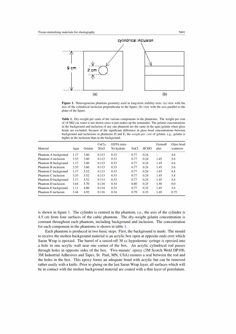
Figure 4. Mean storage moduli and standard errors for phantoms A and B. Production samplevalues are shown over a period of 1 year as filled triangles, circles or squares; inclusion valuesare shown as for phantom A and � for phantom B, and background values are shown as • forphantom A and � for phantom B. Mean storage moduli for inclusion samples cut from the phantomsare shown as � for phantom A and � for phantom B. Mean storage moduli for background samplescut from the phantoms are shown as ◦ for phantom A and � for phantom B.

4.3. Geometry

To test for size changes of inclusions due to osmosis, the cylinders were made (at the time ofphantom production) with a diameter of 20.0 mm, and diameter measurements were made onslices cut from the phantoms many months after production as described in subsection 4.1.Typically, four independent inclusion diameter measurements were made with a machinist’scalipers for each slice, and the uncertainty of the mean was taken to be the standard error.Diameter measurements were also made using ultrasound imaging prior to slicing up thephantoms.

5. Results

5.1. Mechanical properties

In figures 4–6, values for storage moduli are shown for the 2.6-cm-diameter, 1-cm-thick discsamples made at the time of production of each phantom component. Initial measurementswere made within a few days of production of the corresponding phantom and continued for9–12 months. The per cent compression was 2–6%.


Figure 5. Mean storage moduli and standard errors for phantoms C and D. Production samplevalues are shown over a period of 12 months (phantom C) or 10 months (phantom D) as filledtriangles, circles or squares; inclusion values are shown as for phantom C and � for phantom D,and background values are shown as • for phantom C and � for phantom D. Mean storage modulifor inclusion samples cut from the phantoms are shown as � for phantom C and � for phantom D.Mean storage moduli for background samples cut from the phantoms are shown as ◦ forphantom C and � for phantom D.

Also shown in figures 4–6 are the storage moduli for samples excised from each phantom9–12 months after production of the phantom. The per cent compression was 2–4%.

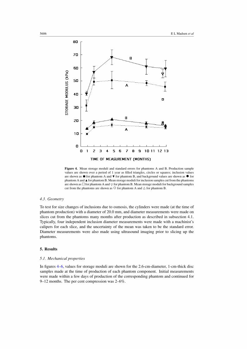
For the production samples corresponding to each type of material, the value of tanδ ≡ (imaginary part of Young’s modulus)/(real part of Young’s modulus) = (loss modulus)/(storage modulus) does not demonstrate a time dependence when the material is at least4 weeks old (see appendix A). Thus, it is considered sufficient to characterize the loss moduliof the production samples in terms of mean values and sample standard deviations over thetime periods indicated in figures 4–6. Those values are given in table 2.

In table 3, means and standard errors of tan δ are shown for 1-cm-thick samples cutfrom the phantoms on one day followed by means and standard errors for 2-cm-thick samplescut the following day. The 2-cm-thick samples were produced to enhance accuracy ofdetermination of complex Young’s moduli.

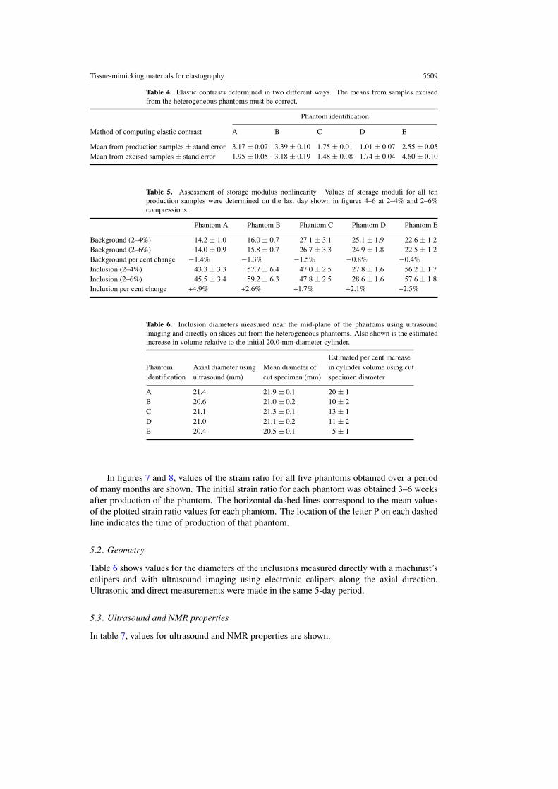
Table 4 shows values of elastic contrasts determined in two ways. The first row of valuescorresponds to means of elastic contrast determined from the values of the storage moduliplotted in figures 4–6 over time. These values resulted from measurements made on the2.6-cm-diameter, 1-cm-thick cylindrical production samples made at the time of productionof each phantom component, i.e., these samples had never existed in one of the phantoms and,therefore, were never exposed to osmotic effects due to contact with materials of different


Figure 6. Mean storage moduli and standard errors for phantom E. Production sample values areshown over a period of nine months as filled circles or squares; inclusion values are shown as ,and background values are shown as •. The mean storage modulus for inclusion samples cutfrom the phantom is shown as �. The mean storage modulus for background samples cut fromthe phantom is shown as ◦.

Table 2. The mean and standard errors of tan δ for the 1- cm-thick production samples over 6–12 months during which (complex) Young’s moduli were measured. Initial tan δ values determinedwithin 4 weeks of the phantom’s production were excluded since they were 10–30% higher thanthe means for the remaining (later) tan δ values.

Phantom A Phantom B Phantom C Phantom D Phantom E

Background 0.108 ± 0.023 0.097 ± 0.007 0.078 ± 0.004 0.070 ± 0.009 0.079 ± 0.007Inclusion 0.121 ± 0.011 0.117 ± 0.010 0.096 ± 0.007 0.110 ± 0.013 0.122 ± 0.005

Table 3. Means and standard errors for tan δ corresponding to 1-cm-thick and 2-cm-thick samplescut from the phantoms. Note that the values for the 1-cm-thick samples are generally considerablygreater than those for the 2-cm-thick samples.


Background (1-cm cuts) 0.098 ± 0.010 0.126 ± 0.010 0.105 ± 0.005 0.121 ± 0.008 0.121 ± 0.008Inclusion (1-cm cuts) 0.157 ± 0.008 0.152 ± 0.006 0.154 ± 0.021 0.154 ± 0.011 0.164 ± 0.009Background (2-cm cuts) 0.095 ± 0.004 0.096 ± 0.004 0.075 ± 0.006 0.078 ± 0.003 0.078 ± 0.005Inclusion (2-cm cuts) 0.119 ± 0.005 0.106 ± 0.017 0.096 ± 0.004 0.108 ± 0.005 0.120 ± 0.005

compositions. The second row of values consists of means of elastic contrast values determinedfrom storage modulus values for the samples cut from slabs of the phantoms. The second rowof values must be the correct values for the phantoms, of course.

There was a small nonlinearity in storage moduli observed. This was quantified bycomparing measurements at 2–4% and 2–6% compressions on the same samples on the sameday (the last day in figures 4–6). The results are shown in table 5.


Table 4. Elastic contrasts determined in two different ways. The means from samples excisedfrom the heterogeneous phantoms must be correct.

Phantom identification

Method of computing elastic contrast A B C D E

Mean from production samples ± stand error 3.17 ± 0.07 3.39 ± 0.10 1.75 ± 0.01 1.01 ± 0.07 2.55 ± 0.05Mean from excised samples ± stand error 1.95 ± 0.05 3.18 ± 0.19 1.48 ± 0.08 1.74 ± 0.04 4.60 ± 0.10

Table 5. Assessment of storage modulus nonlinearity. Values of storage moduli for all tenproduction samples were determined on the last day shown in figures 4–6 at 2–4% and 2–6%compressions.


Background (2–4%) 14.2 ± 1.0 16.0 ± 0.7 27.1 ± 3.1 25.1 ± 1.9 22.6 ± 1.2Background (2–6%) 14.0 ± 0.9 15.8 ± 0.7 26.7 ± 3.3 24.9 ± 1.8 22.5 ± 1.2Background per cent change −1.4% −1.3% −1.5% −0.8% −0.4%Inclusion (2–4%) 43.3 ± 3.3 57.7 ± 6.4 47.0 ± 2.5 27.8 ± 1.6 56.2 ± 1.7Inclusion (2–6%) 45.5 ± 3.4 59.2 ± 6.3 47.8 ± 2.5 28.6 ± 1.6 57.6 ± 1.8Inclusion per cent change +4.9% +2.6% +1.7% +2.1% +2.5%

Table 6. Inclusion diameters measured near the mid-plane of the phantoms using ultrasoundimaging and directly on slices cut from the heterogeneous phantoms. Also shown is the estimatedincrease in volume relative to the initial 20.0-mm-diameter cylinder.

Estimated per cent increasePhantom Axial diameter using Mean diameter of in cylinder volume using cutidentification ultrasound (mm) cut specimen (mm) specimen diameter

A 21.4 21.9 ± 0.1 20 ± 1B 20.6 21.0 ± 0.2 10 ± 2C 21.1 21.3 ± 0.1 13 ± 1D 21.0 21.1 ± 0.2 11 ± 2E 20.4 20.5 ± 0.1 5 ± 1

In figures 7 and 8, values of the strain ratio for all five phantoms obtained over a periodof many months are shown. The initial strain ratio for each phantom was obtained 3–6 weeksafter production of the phantom. The horizontal dashed lines correspond to the mean valuesof the plotted strain ratio values for each phantom. The location of the letter P on each dashedline indicates the time of production of that phantom.

5.2. Geometry

Table 6 shows values for the diameters of the inclusions measured directly with a machinist’scalipers and with ultrasound imaging using electronic calipers along the axial direction.Ultrasonic and direct measurements were made in the same 5-day period.

5.3. Ultrasound and NMR properties

In table 7, values for ultrasound and NMR properties are shown.


Figure 7. Strain ratios obtained from elastograms over a 10 month period for phantom A (•),phantom B ( ) and phantom C (�). The dashed horizontal lines correspond to the mean of allstrain ratios for each phantom, the numerical value appearing on the right side. The position of theletter P on each dashed line indicates the time of production of the phantom.

Table 7. Ultrasound and NMR properties measured at 22 ◦C on samples of each of the ten differentmaterials formed at the time of production of each material. Density values were computed basedon knowledge of densities of component materials.

Ultrasound properties NMR relaxation times

Propagation Atten. coeff. ÷ frequency Density T1 T2

TM material version speed (m s−1) (dB cm−1 MHz−1) (g ml−1) (ms) (ms)

Phantom A BKGD 1518 ± 1 0.35 ± 0.02 1.04 498.2 ± 0.2 63 ± 2Phantom A INCL 1527 ± 1 0.45 ± 0.02 1.05 431 ± 5 28.4 ± 0.2Phantom B BKGD 1526 ± 1 0.35 ± 0.02 1.04 456.6 ± 0.5 60 ± 2Phantom B INCL 1533 ± 1 0.47 ± 0.02 1.05 402.3 ± 0.4 28.8 ± 0.3Phantom C BKGD 1532 ± 1 0.36 ± 0.02 1.04 419 ± 1 59 ± 1Phantom C INCL 1542 ± 1 0.50 ± 0.02 1.05 369 ± 1 32.7 ± 0.5Phantom D BKGD 1532 ± 1 0.38 ± 0.02 1.04 423.0 ± 0.8 57 ± 1Phantom D INCL 1535 ± 1 0.14 ± 0.02 1.00 494 ± 2 59 ± 1Phantom E BKGD 1518 ± 1 0.46 ± 0.02 1.04 396 ± 1 59 ± 1Phantom E INCL 1518 ± 1 0.18 ± 0.02 1.00 488 ± 1 53 ± 1


Figure 8. Strain ratios obtained from elastograms over a 9 month period for phantom D (◦) anda 7 month period for phantom E (�). The dashed horizontal lines correspond to the mean of allstrain ratios for each phantom, excluding the initial values in each case. The numerical mean valuecorresponding to the dashed line appears at the right end of the line. The position of the letter P oneach dashed line indicates the time of production of the phantom.

6. Discussion

6.1. Storage moduli

The storage moduli of the production samples (produced at the time of production of eachphantom component) are shown over a 9 to 12 month period in figures 4–6 (closed circles,triangles and squares). The storage moduli rise considerably during the first few months andthen gradually decrease.

The storage moduli for the samples cut from the phantoms are also shown in figures 4–6(open circles, triangles and squares). Those storage moduli of samples cut from thebackgrounds agree rather well with those of the background production samples measured atthe same time. However, for storage moduli of the inclusions that level of agreement existsonly for phantoms B and C. Assuming that the (mean) storage modulus for the inclusionsamples cut from the phantom is the correct value, the production sample values for phantomsA, D and E are, respectively, high by 27%, low by 47% and low by 45%. Thus, values ofstorage moduli for the inclusion production samples should not be assumed to correspond tothe storage moduli of the inclusion material in the actual phantom.

In figure 5, the values of storage moduli measured over time for the inclusion productionsamples for phantom D are confusing. Based on compositions, the inclusion storage moduli


might be expected to be nearly the same as those for phantom C. As seen in table 1, themajor difference in composition between phantoms C and D is that there are no beads in theinclusion material of phantom D, while there are beads in the inclusion material of phantom C.The inclusion storage moduli for phantom D (figure 5) are far below those for phantom C.In fact, earlier inclusion storage moduli for phantom D are lower than the correspondingbackground values and end up only slightly higher. On the other hand, the mean storagemoduli for inclusion samples cut from phantom D agree with both cut and production samplesfor phantom C, as would be expected. One possible explanation for the unexpected storagemodulus values for the inclusion production samples of phantom D is that there was a mix upof samples in the laboratory, i.e., the production samples measured did not actually correspondto the inclusion material in phantom D. Another possible explanation is that the two productionsamples corresponding to the inclusion material of phantom D were accidentally placed closeto a laboratory heating source and their temperature became elevated enough to cause chemicalchange with no visual evidence that heating had occurred.

A small nonlinearity was observed for the storage moduli when results for a compressionrange of 2–4% were compared with results for a range of 2–6% (table 5). An average decreaseof about 1% for the five background samples occurred with higher compression range whilean increase of about 2.8% occurred for the five inclusion samples. (However, excludingphantom A from the average, the average increase for the inclusion samples was 2.2%.) Thehigher dry-weight concentration of agar in the inclusions may account for the increase for theinclusion samples, agar per se being nonlinear (Hall et al 1997).

The lack of validity of inclusion storage moduli of the production samples is reflected inthe computed elastic contrast values shown in table 4. The elastic contrasts computed fromthe storage moduli of the samples cut from the samples should be the correct values for thephantoms.

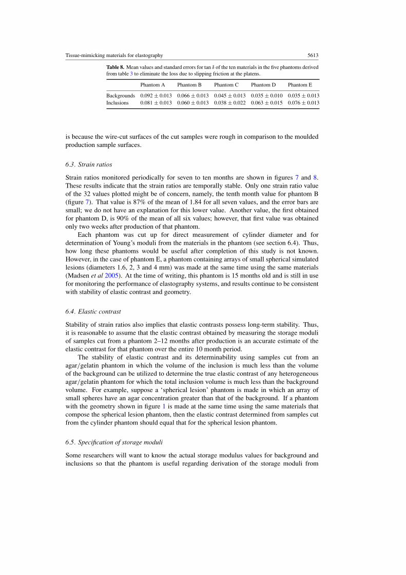
6.2. Loss moduli and tan δ values

Referring to table 3, where tan δ values are shown for 1-cm-thick and 2-cm-thick samples cutfrom the phantoms, tan δ values for the 1-cm-thick samples are generally considerably greaterthan those for the 2-cm-thick samples, even though the storage moduli for the 1-cm and 2-cmsamples agree very well for each of the ten different materials. Thus, there is a significantpartial loss due to slipping friction at the platens, and that part of the loss should not be countedin the loss moduli or tan δ values.

The correct values of the loss modulus—or equivalently tan δ—can be computed fromthe values in table 3 using the following facts: (1) The ratio of the amplitude of the sinusoidaloscillation to the sample thickness was kept the same, namely, 0.01. (2) The parallel flat areascontacting the platens were all the same. (3) The Young’s modulus is an intrinsic materialproperty. The applicable relations are

E′′ = 2E′′2-cm − E′′

1-cm and tan δ = 2 tan δ2-cm − tan δ1-cm (1)

where E′′ and tan δ are the computed best estimates for the loss modulus and tan δ, E′′1-cm

is the loss modulus determined experimentally using the 1-cm-thick cut sample, etc (seeappendix B for a derivation of equations (1)). With propagation of errors, the corrected(computed) mean values and standard errors of tan δ are given in table 8.

The derived (corrected) values of tan δ for phantom A are a little larger than for the otherfour phantoms. Recall that all phantoms except phantom A were preserved with Germall-plus R©, phantom A being preserved with thimerosal.

Note that the measured tan δ values for the production samples shown in table 2 are lessthan those for the equal thickness (1 cm) samples cut from the phantom (table 3). This likely


Table 8. Mean values and standard errors for tan δ of the ten materials in the five phantoms derivedfrom table 3 to eliminate the loss due to slipping friction at the platens.


Backgrounds 0.092 ± 0.013 0.066 ± 0.013 0.045 ± 0.013 0.035 ± 0.010 0.035 ± 0.013Inclusions 0.081 ± 0.013 0.060 ± 0.013 0.038 ± 0.022 0.063 ± 0.015 0.076 ± 0.013

is because the wire-cut surfaces of the cut samples were rough in comparison to the mouldedproduction sample surfaces.

6.3. Strain ratios

Strain ratios monitored periodically for seven to ten months are shown in figures 7 and 8.These results indicate that the strain ratios are temporally stable. Only one strain ratio valueof the 32 values plotted might be of concern, namely, the tenth month value for phantom B(figure 7). That value is 87% of the mean of 1.84 for all seven values, and the error bars aresmall; we do not have an explanation for this lower value. Another value, the first obtainedfor phantom D, is 90% of the mean of all six values; however, that first value was obtainedonly two weeks after production of that phantom.

Each phantom was cut up for direct measurement of cylinder diameter and fordetermination of Young’s moduli from the materials in the phantom (see section 6.4). Thus,how long these phantoms would be useful after completion of this study is not known.However, in the case of phantom E, a phantom containing arrays of small spherical simulatedlesions (diameters 1.6, 2, 3 and 4 mm) was made at the same time using the same materials(Madsen et al 2005). At the time of writing, this phantom is 15 months old and is still in usefor monitoring the performance of elastography systems, and results continue to be consistentwith stability of elastic contrast and geometry.

6.4. Elastic contrast

Stability of strain ratios also implies that elastic contrasts possess long-term stability. Thus,it is reasonable to assume that the elastic contrast obtained by measuring the storage moduliof samples cut from a phantom 2–12 months after production is an accurate estimate of theelastic contrast for that phantom over the entire 10 month period.

The stability of elastic contrast and its determinability using samples cut from anagar/gelatin phantom in which the volume of the inclusion is much less than the volumeof the background can be utilized to determine the true elastic contrast of any heterogeneousagar/gelatin phantom for which the total inclusion volume is much less than the backgroundvolume. For example, suppose a ‘spherical lesion’ phantom is made in which an array ofsmall spheres have an agar concentration greater than that of the background. If a phantomwith the geometry shown in figure 1 is made at the same time using the same materials thatcompose the spherical lesion phantom, then the elastic contrast determined from samples cutfrom the cylinder phantom should equal that for the spherical lesion phantom.

6.5. Specification of storage moduli

Some researchers will want to know the actual storage modulus values for background andinclusions so that the phantom is useful regarding derivation of the storage moduli from


strain ratios. If production samples corresponding to the background material are madeand it is accepted that the elastic contrast is invariant, then determination of the elasticcontrast using samples cut from a cylinder phantom plus the value of the storage modulusof the background at the time of concern allow computation of the storage modulus of theinclusion(s).

6.6. Geometry

Referring to table 6, all cylindrical inclusions increased in diameter from an initial value of20.0 mm at the time of production. The greatest diameter increase occurred for phantom A.Phantom A is not very important, however, because the preservative used was thimerosal, amercury-containing compound used in past phantoms. The more environmentally acceptableGermall-plus has been shown to be an excellent alternative to thimerosal; therefore, futurephantoms will be preserved with Germall-plus instead of thimerosal. The mean diameterincrease for phantoms B–D was 1 mm, about 5%, and the mean volume increase was10%. These are small increases. Thus, if a spherical lesion phantom were produced with3.0-mm-diameter spherical inclusions, then a sphere volume increase of 10% corresponds toa diameter increase from 3.0 to 3.1 mm, a tolerable difference.

The fact that no perceptible changes in size of inclusions were observed for low MRcontrast phantoms (Madsen et al 1991) described in section 1 may be related to two factors:first, the MR phantoms were low contrast so that the dry-weight agar concentrations in theinclusions were closer to that in the surroundings than in the present study; second, theuncertainties in the MR determinations of sizes were greater than in the case of modernultrasound or direct measurement with machinist’s calipers done in the current study.

6.7. Ultrasound properties

Since the values for these properties were measured on ‘production’ samples made at thetime of production of the respective phantom components, only values for the backgroundmaterials can be assumed accurate. However, since the increases in volume of inclusions inthe phantoms are only about 10%, it is reasonable that ultrasound properties determined for theinclusion materials are not greatly in error. If more accurate values of ultrasound attenuationcoefficients and propagation speed for the inclusion material are considered essential for someuse of the phantom, then samples cut from the cylinder phantom for determination of Young’smoduli could also be used to measure those ultrasound properties.

Note that the slopes of the ultrasound attenuation coefficient versus frequency for thebackground materials of all five phantoms lie in the range 0.35–0.46 dB cm−1 MHz−1 at22 ◦C, a good approximation for the attenuation of many soft tissues.

The ultrasound propagation speeds in the background materials range from 1518 through1532 m s−1 at 22 ◦C. If values closer to 1540 m s−1 are desired, an appropriate concentrationof glycerol can be included in both background and inclusions during manufacture of thephantom.

We have used small concentrations of glycerol to raise propagation speeds in ultrasoundphantom materials. The rate of increase is about 4.4 m s−1 per weight per cent glycerol. Forweight per cent concentrations of up to 10%, the increase in attenuation coefficient slope isless than 0.02 dB cm−1 MHz−1. To adjust a speed from 1518 m s−1 to 1540 m s−1 wouldrequire a 5% glycerol concentration. Thus, ultrasound attenuation should not be affected.It seems likely that mechanical properties would not be significantly affected at this lowconcentration either.


6.8. NMR properties

In the case of phantoms A, B and C, both T1 and T2 are lower for the inclusion material thanfor the background material. This is expected because of the higher concentration of agar inthe inclusion material. However, this expected distinction between inclusion and backgroundmaterials is not demonstrated for phantoms D and E. For these phantoms, T1 actually is higherin the inclusions than in the background and T2 is about the same.

A major difference between the phantoms is that in phantoms A–C the inclusions havea rather high concentration of glass beads (about 5.5% by weight), while there are no beadsin the inclusion of phantom D and a relatively small concentration in the inclusion ofphantom E (see table 1). All five phantoms have a bead concentration of 3.4–4.6% byweight in the backgrounds. Probably the glass beads contribute to lowering T1 and T2. If themagnetic susceptibility of the glass beads is sufficiently different from that of the surroundinggel, then the T2 value measured is actually T ∗

2 , which depends on settings of the pulse spacingof the CPMG pulse sequence. Thus, T ∗

2 is not an acceptable specification of the T2 intrinsicto materials.

An experiment was carried out on a sample with a higher concentration of glass beads(inclusion material for phantom B) to see if the measured T2 value depended on the CPMGpulse separation. Using the usual pulse separation of 2.5 ms, the T2 value was 27.4 ms. Withpulse separations of 1 ms, 0.2 ms and 0.1 ms, the T2 values determined were 31.3 ms, 39 msand 41 ms, respectively, indicating that the beads were lowering measured T2 values dueto diffusion effects and non-tissue-like local variations in magnetic permeability. Thus, ifphantoms are to be considered tissue-mimicking for use in MR elastography, there should beno glass beads present.

7. Summary and conclusions

Five phantoms with a variety of compositions were made using a base material of agar,gelatin, water, formaldehyde, Cu2+, EDTA, NaCl, microscopic glass beads and a preservative.Cylindrical inclusions existed in each phantom with higher dry-weight agar concentrations thanin the background material. The dry-weight gelatin concentration was constant throughouteach phantom. The volume fraction corresponding to the cylindrical inclusions was small—about 4%. The phantoms are tissue-mimicking with respect to mechanical and ultrasoundproperties, but adequate mimicking of NMR relaxation times is compromised by the presenceof microscopic glass beds used to increase ultrasound attenuation. Agar/gelatin phantoms foruse in MR elastography should be made without glass beads.

Changes in the inclusions for about 1 month following production were probably causedby osmotic effects. These changes included an approximately 10% increase in cylindervolume and a significant change in Young’s modulus compared to the value for samples ofinclusion material not subject to osmotic effects (never in contact with background material).Thus, the true Young’s modulus of the cylindrical inclusion must be determined using asample cut from the phantom.

Note that tan δ for the materials in these phantom materials is small—about 0.05.Monitoring of the strain ratio for the five phantoms over 7–10 months indicated long-term

stability of that parameter. Stability of strain ratio implies stability of elastic contrast also.Thus, elastic contrast for a phantom can be determined by measuring the storage modulus ofinclusion and background materials excised from the phantom, allowing 1 or 2 months afterproduction of the phantom for chemical stability to be established.


7.1. Characterization of phantoms with inclusions of any size and number buta small total volume fraction

Phantoms for testing the performance of elastography systems are not restricted to oneswith cylindrical inclusions. For example, one type of phantom (Madsen et al 2004) hasarrays of small spherical inclusions in a background material, the total volume fraction ofinclusions being much less than 4%. It is not practical to try to measure the inclusion storagemodulus using samples cut from the small spheres since the spheres are 5 mm or less indiameter. However, if a phantom of the geometry in figure 1 is made at the same time asthe spherical lesion phantom with the background and 2-cm inclusion diameter cylindricalinclusion composed of the same materials as in the spherical lesion phantom, then samplescan be cut from the cylinder phantom after 2 months to determine the storage modulusof background and inclusion and, therefore, the elastic contrast for both the cylinder andspherical lesion phantom.

Some researchers in elastography are interested in deriving the storage modulusdistribution using the strain ratio elastogram. Following is a method for determining thestorage moduli for background and inclusions in these phantoms at any time followingproduction of the phantom. Although the elastic contrast in the phantoms is stable, theactual values of the storage moduli for the background material rise and then fall over atleast a year. (See background storage moduli in figures 4–6.) If samples of backgroundmaterial for measurement of the storage modulus are produced at the time of production ofa phantom, a measurement of the storage modulus of these background samples at any time,plus knowledge of the elastic contrast, allows computation of the storage modulus of theinclusion material at that time.

7.2. Method of preservation

There appears to be no advantage to the use of thimerosal as a preservative while thereis a considerable disadvantage since thimerosal is a mercury-containing compound. Thus,preservation with Germall-Plus R© is recommended.

Acknowledgments

Work supported in part by NIH grants R01EB000459 and R21 EB003853 and by WhitakerFoundation grant RG-02–0457.

Appendix A

Values of tan δ versus time after production are given in table A1 for the phantom Cproduction samples. These demonstrate the lack of time dependence of tan δ when thesamples are at least 4 weeks old. Note that the largest values for both background andinclusion occur at 1 week after production.

Appendix B

There is an error in the measured loss modulus, E′′, and therefore also in tan δ due to slippingfriction at the interface between the platens and sample. Following is a way to computecorrected values of E′′ and tan δ when measurements of Young’s moduli of samples differingonly in thickness are available. Samples with the same area and thicknesses of 1 cm and 2 cm


Table A1. Values of tan δ versus time lapse since production for the production samplescorresponding to phantom C.

Number of weeks after production ofthe phantom and production samples

Material 1 6 14 41 52

Background 0.087 0.073 0.078 0.083 0.077Inclusion 0.121 0.103 0.094 0.087 0.098

cut from the phantoms were available. The per cent compression range used for both was thesame, namely, 2–4%. The (complex) Young’s modulus E is defined by

�F/A = E�z/z (B.1)

where �F is the sinusoidally varying force, A is the mean sample area, �z is thesinusoidally varying displacement and z is the sample thickness. For notational brevity,define �P ≡ �F/A and �C ≡ �z/z. Then equation (B.1) becomes

�P = E�C. (B.2)

We have �P = (�P )o eiωt and �C = (�C)o ei(ωt−δ), δ � 0, where δ is the phase lag ofdisplacement due to energy loss in the material. Then

E = �P/�C = (�P )o/(�C)o eiδ = E′ + iE′′ (B.3)

where (�P )o and (�C)o correspond to real-valued amplitudes, E′ is the (real) storagemodulus, E′′ is the (real) loss modulus and i ≡ √−1. Also, tan δ = E′′/E′.

The energy loss per cycle for a disc of mean area A and mean thickness z, not countingslipping frictional loss at the platens, can be computed as a function of E′′ and (�C)o.Consider the real force applied by the platen at the one moving surface �FR = (�P )oA cos ωt

(The other surface is assumed to be stationary) and the real displacement at that surface�zR = (�C)o z cos(ωt − δ). Thus the energy loss per cycle, ignoring frictional loss at theplatens, is

L =∫

one cycle�FRd(�zR)

= −(�P )oA(�C)ozω

∫ 2π/ω

0cos(ωt) sin(ωt − δ) dt

= (�P )oA(�C)ozπ sin δ, (B.4)

and the loss per cycle per unit volume, ignoring friction at the platens, is

L/(Az) = (�P )o(�C)oπ sin δ = πE′′(�C)2o (B.5)

where E′′ = (�P )o/(�C)o sin δ has been imported from equation (B.3).Since the values of A and (�C)o are assumed to have been made the same experimentally

for samples of different thicknesses, the energy loss per cycle due to slipping friction at theplatens, LF, must be the same for both thicknesses. Let the thickness of one sample, z2, betwice the thickness of the other sample, z1; then z2 = 2z1. Thus, the actual energy loss percycle, including slipping frictional loss at the platens, is L2 = (�P )o A(�C)oz2π sin δ + LF

for the sample of thickness z2 and L1 = (�P )o A(�C)oz1π sin δ + LF for the sample ofthickness z1.


The measured loss moduli are

E′′1 = [

π(�C)2o

]−1[(L1 + LF)/(Az1)] = E′′ + LF

[π(�C)2

oAz1]−1

(B.6)

and

E′′2 = [

π(�C)2o

]−1[(L2 + LF)/(Az1)] = E′′ + LF

[π(�C)2

oAz2]−1

(B.7)

for sample thicknesses z1 and z2, respectively, where E′′ is the correct loss modulus.Introducing the assumption that z2 = 2z1, equations (B.6) and (B.7) can be solved for the

correct loss modulus, E′′ in terms of E′′1 and E′′

2, namely,

E′′ = 2E′′2 − E′′

1 . (B.8)

If the storage moduli determined for the two thicknesses are the same (They were for the 1-cmand 2-cm-thick cut samples.) and are assumed to be correct, then

E′′/E′ = 2E′′2 /E′ − E′′

1 /E′ or tan δ = 2 tan δ2 − tan δ1 (B.9)

where tan δ1 corresponds to the measured value for the sample of thickness z1 and tan δ2

corresponds to the measured value for the sample of thickness z2.

References

Bevington P R 1969 Data Reduction and Error Analysis for the Physical Sciences (New York: McGraw-Hill)de Korte C L, Cespedes E L, van der Steen A F W, Norder B and te Nijenhuis K 1997 Elastic and acoustic properties

of vessel mimicking material for elasticity imaging Ultrason. Imaging 19 112–26Gao L, Parker K J and Alam S K 1995 Sonoelasticity imaging: theory and experimental verification J. Acoust. Soc.

Am. 97 3875–86Hall T J, Bilgen M, Insana M F and Krouskop T A 1997 Phantom materials for elastography IEEE Trans. Ultrason.

Ferroelectr. Freq. Control 44 1355–65Kallel F, Prihoda C D and Ophir J 2001 Contrast-transfer efficiency for continuously varying tissue moduli: simulation

and phantom validation Ultrasound Med. Biol. 27 1115–25Madsen E L, Blechinger J C and Frank G R 1991 Low-contrast focal lesion detectability phantoms for 1H MR imaging

Med. Phys. 18 549–54Madsen E L et al 1999 Interlaboratory comparison of ultrasonic backscatter, attenuation and speed J. Ultrasound

Med. 18 615–31Madsen E L et al 2004 Tissue-mimicking spherical lesion phantoms for elastography with and without ultrasound

refraction effects Proc. Third Int. Conf. on the Ultrasonic Measurement and Imaging of Tissue Elasticity(Lake Windermere, Cumbria 17–20 Oct 2004) p 102

Madsen E L, Frank G R, Hobson M A, Shi H, Jiang J, Varghese T and Hall T J 2005 Spherical lesion phantoms fortesting the performance of elastography systems Phys. Med. Biol. submitted

Madsen E L, Frank G R, Krouskop T A, Varghese T, Kallel F and Ophir J 2003 Tissue-mimicking oil-in-gelatindispersions for use in heterogeneous phantoms Ultrason. Imaging 25 17–38

Plewes D B, Bishop J, Samani A and Sciarretta J 2000 Visualization and quantification of breast cancer bio-mechanicalproperties with magnetic resonance elastography Phys. Med. Biol. 45 1591–610

Rice J R, Milbrandt R H, Madsen E L, Frank G R and Boote E J 1998 Anthropomorphic 1H MRS head phantomMed. Phys. 25 1145–56

Documents

Tissue-mimicking agar gelatin materials for use in ... · Tissue-mimicking materials for elastography 5599 Long-term stability of lesion diameters and T 2 relaxation times in the