Tire Pressure Maintenance - A Statistical Investigation

DOT HS 811 086 April 2009

Tire Pressure Maintenance -A Statistical Investigation

This report is free of charge from the NHTSA Web site at www.nhtsa.dot.gov

This publication is distributed by the U.S. Department of Transportation, National Highway Traffic Safety Administration, in the interest of information exchange. The opinions, findings and conclusions expressed in this publication are those of the author(s) and not necessarily those of the Department of Transportation or the National Highway Traffic Safety Administration. The United States Government assumes no liability for its content or use thereof. If trade or manufacturers’ names or products are mentioned, it is because they are considered essential to the object of the publication and should not be construed as an endorsement. The United States Government does not endorse products or manufacturers.

1. Report No. DOT HS 811 086

2. Government Accession No.

3. Recipient's Catalog No.

5. Report Date April 2009

4. Title and Subtitle Tire Pressure Maintenance – A Statistical Investigation 6. Performing Organization Code

7. Author(s) Santokh Singh*, Kristin Kingsley, Chou-Lin Chen

8. Performing Organization Report No. 10. Work Unit No. (TRAIS)

9. Performing Organization Name and Address National Highway Traffic Safety Administration 1200 New Jersey Avenue SE. Washington, DC 20590 *URC Enterprises, Inc.

11. Contract or Grant No.

13. Type of Report and Period Covered NHTSA Technical Report

12. Sponsoring Agency Name and Address Mathematical Analysis Division, National Center for Statistics and Analysis National Highway Traffic Safety Administration 1200 New Jersey Avenue SE. Washington, DC 20590 14. Sponsoring Agency Code

15. Supplementary Notes 16. Abstract Past studies on tire pressure monitoring have revealed that about 28 percent of light vehicles on our Nation's roadways run with at least one underinflated tire. Only a few psi difference from vehicle manufacturer's recommended tire inflation pressure can affect a vehicle's handling and stopping distance. Poor tire maintenance can increase incidences of blowouts and tread separations. Similarly, underinflation negatively affects fuel economy. In 2005, NHTSA's FMVSS 138 required automobile manufacturers to install tire pressure monitoring systems (TPMS) on light passenger vehicles with phase-in period from 2006 to 2008. Prior to the regulation, NHTSA’s National Center for Statistics and Analysis conducted several surveys and studies to estimate and compare the benefits of Direct and Indirect TPMS. The results of the most recently conducted survey, Tire Pressure Monitoring System Study, are presented in this report. Data collection in this survey ceased prior to its completion. This study outlines a Bayesian approach to compute the case weights so that the estimates could be representative of the universe considered for the survey. Subsequently, effectiveness of TPMS is studied by comparing estimates of percentages of underinflated and overinflated vehicles with and without TPMS, as well as the average underinflation and overinflation over vehicles in the two groups: vehicles with and without TPMS. Testing some relevant hypotheses provides statistical support to claims made in favor of TPMS based on the above comparisons. The analysis also covers comparison of direct and indirect versions of TPMS, concluding that direct type of TPMS is more effective as compared with the indirect. Since this data collection, improvements have been made to both kinds of TPMS, so different results are to be expected if the study were to be conducted presently. 17. Key Words Tire pressure, Case weights, Underinflation, Overinflation.

18. Distribution Statement This report is free of charge from the NHTSA Web site at www.nhtsa.dot.gov

19. Security Classif. (of this report) Unclassified

20. Security Classif. (of this page) Unclassified

21. No. of Pages 19

22. Price

http://www.nhtsa.dot.gov/

Contents

1 INTRODUCTION 1

2 DATA COLLECTION METHODOLOGY 1

3 TARGET INFORMATION (DATA) 2

4 SAMPLE SIZE 2

5 SAMPLE DESIGN AND CASE WEIGHTS 3

6 ANALYSIS 5

6.1 Preliminary Analysis . . . . . . . . . . . . . . . . . . . . . . . . . . . . . . . . . . . . . . 6

6.2 Analysis: Comparison of Vehicle Groups and Their Subcategories . . . . . . . . . . . 7

6.2.1 Correct Pressure . . . . . . . . . . . . . . . . . . . . . . . . . . . . . . . . . . . . . 8

6.2.2 Underinflation . . . . . . . . . . . . . . . . . . . . . . . . . . . . . . . . . . . . . . 8

6.2.3 Overinflation . . . . . . . . . . . . . . . . . . . . . . . . . . . . . . . . . . . . . . . 9

7 TPMS EFFECTIVENESS ANALYSIS 10

7.1 Effectiveness - Controlling Underinflation . . . . . . . . . . . . . . . . . . . . . . . . . . . 11

7.2 Effectiveness - Controlling Overinflation . . . . . . . . . . . . . . . . . . . . . . . . . . . . 11

8 RESULTS AND DISCUSSION 12

9 APPENDIX 13

i

_________________________________________________________________________________________________________ NHTSA's National Center for Statistics and Analysis, 1200 New Jersey Avenue SE., Washington, DC 2590

List of Figures

1 Comparison-actual sample sizes and planned sample sizes for the 24 selected PSUs . . . . . . . . 3

2 Percent frequency distributions of Underinflated and Overinflated vehicles . . . . . . . . . . . . 7

3 Percent vehicles with Underinflation and Overinflation exceeding threshold values, 0, 5, 10, 25,

35, 45 percent. . . . . . . . . . . . . . . . . . . . . . . . . . . . . . . . . . . . . . . . . . . . 8

ii


List of Tables

1 Sample segmentation by vehicle groups and their subcategories . . . . . . . . . . . . . . . . . . 2

2 Stratification in an exemplar PSU. . . . . . . . . . . . . . . . . . . . . . . . . . . . . . . . . . 4

3 Allocation of sampled vehicles and their estimates over vehicle groups . . . . . . . . . . . . . . 5

4 Underinflation status by vehicle group and device type . . . . . . . . . . . . . . . . . . . . . . 9

5 Average underinflation (percent) by vehicle group and device type . . . . . . . . . . . . . . . . 10

6 Overinflation status by vehicle group and device type . . . . . . . . . . . . . . . . . . . . . . . 10

7 Average Overinflation (percent) by vehicle group and device type . . . . . . . . . . . . . . . . . 11

iii


iv


EXECUTIVE SUMMARY

Background and Objective

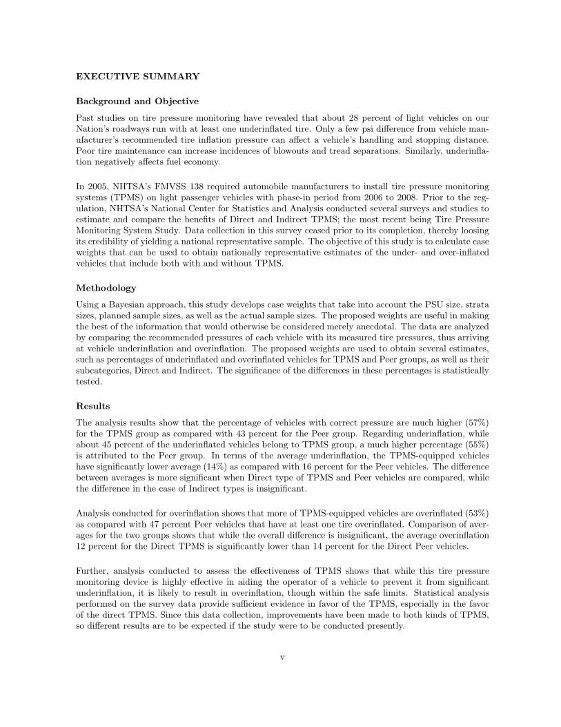
Past studies on tire pressure monitoring have revealed that about 28 percent of light vehicles on ourNation’s roadways run with at least one underinflated tire. Only a few psi difference from vehicle man-ufacturer’s recommended tire inflation pressure can affect a vehicle’s handling and stopping distance.Poor tire maintenance can increase incidences of blowouts and tread separations. Similarly, underinfla-tion negatively affects fuel economy.

In 2005, NHTSA’s FMVSS 138 required automobile manufacturers to install tire pressure monitoringsystems (TPMS) on light passenger vehicles with phase-in period from 2006 to 2008. Prior to the reg-ulation, NHTSA’s National Center for Statistics and Analysis conducted several surveys and studies toestimate and compare the benefits of Direct and Indirect TPMS; the most recent being Tire PressureMonitoring System Study. Data collection in this survey ceased prior to its completion, thereby loosingits credibility of yielding a national representative sample. The objective of this study is to calculate caseweights that can be used to obtain nationally representative estimates of the under- and over-inflatedvehicles that include both with and without TPMS.

Methodology

Using a Bayesian approach, this study develops case weights that take into account the PSU size, stratasizes, planned sample sizes, as well as the actual sample sizes. The proposed weights are useful in makingthe best of the information that would otherwise be considered merely anecdotal. The data are analyzedby comparing the recommended pressures of each vehicle with its measured tire pressures, thus arrivingat vehicle underinflation and overinflation. The proposed weights are used to obtain several estimates,such as percentages of underinflated and overinflated vehicles for TPMS and Peer groups, as well as theirsubcategories, Direct and Indirect. The significance of the differences in these percentages is statisticallytested.

Results

The analysis results show that the percentage of vehicles with correct pressure are much higher (57%)for the TPMS group as compared with 43 percent for the Peer group. Regarding underinflation, whileabout 45 percent of the underinflated vehicles belong to TPMS group, a much higher percentage (55%)is attributed to the Peer group. In terms of the average underinflation, the TPMS-equipped vehicleshave significantly lower average (14%) as compared with 16 percent for the Peer vehicles. The differencebetween averages is more significant when Direct type of TPMS and Peer vehicles are compared, whilethe difference in the case of Indirect types is insignificant.

Analysis conducted for overinflation shows that more of TPMS-equipped vehicles are overinflated (53%)as compared with 47 percent Peer vehicles that have at least one tire overinflated. Comparison of aver-ages for the two groups shows that while the overall difference is insignificant, the average overinflation12 percent for the Direct TPMS is significantly lower than 14 percent for the Direct Peer vehicles.

Further, analysis conducted to assess the effectiveness of TPMS shows that while this tire pressuremonitoring device is highly effective in aiding the operator of a vehicle to prevent it from significantunderinflation, it is likely to result in overinflation, though within the safe limits. Statistical analysisperformed on the survey data provide sufficient evidence in favor of the TPMS, especially in the favorof the direct TPMS. Since this data collection, improvements have been made to both kinds of TPMS,so different results are to be expected if the study were to be conducted presently.

v

vi

1 INTRODUCTION

In order for a vehicle to handle safely and use fuel economically, proper tire inflation, as recommended bythe vehicle manufacturer, needs to be maintained in a vehicle’s tires. Pressure below the recommendedpressure (i.e., underinflation) can cause high heat generation that in turn can cause rapid tire wear,tire blowout, and loss of vehicle control that may cause a crash. TPMS is believed to be an effectivemeans to monitor the tire pressure - a claim that is statistically tested in this study. Comparison ofvehicles equipped with TPMS with the vehicles without TPMS can throw light on the effectiveness ofthis device. Further, there are two types of TPMS, Direct and Indirect. Direct systems operate witha tire pressure sensor in each tire cavity, while Indirect systems monitor tire pressure by comparingcharacteristics of tires, such as wheel speeds using the anti-lock braking system. Indirect systems do notdistinguish between overinflation and underinflation. Therefore, it is also of interest to assess whetherDirect TPMS is more effective as compared with Indirect TPMS.

In support of rulemaking activities mandated by Section 13 of the TREAD Act, the National HighwayTraffic Safety Administration’s National Center for Statistics and Analysis conducted the Tire PressureSpecial Study (TPSS) and the Tire Pressure Monitoring System Study (TPMSS). The TPSS was de-signed to assess to what extent passenger vehicle operators are aware of the recommended tire pressuresfor their vehicles, the frequency and the means they use to measure their tire pressure, and how signifi-cantly the actual measured tire pressure deviated from the manufacturer’s recommended pressure. Thisstudy is focused on the last aspect of the tire pressure maintenance.

The TPMSS was designed to gather tire-pressure-related information on vehicles equipped with differentkinds of tire pressure monitoring systems so that their respective effectiveness could be evaluated. Themain objective was to assess the effectiveness of TPMS, in general and investigate if Direct TPMS is moreeffective as compared with Indirect TPMS. The present study conducts statistical analysis to estimatesome tire-pressure-related statistics, as well as make inferences about the effectiveness of TPMS devices.Section 2 of this paper discusses data collection methodology. In section 3 details about the data collectedin TPMSS are provided. The break-up of the population size and the size of the actual sample collectedin TPMSS is discussed in section 4. Section 5 probes the issue of assigning case weights and outlinesstatistical methodology used in revising weights that is required due to early termination of the survey.Section 6 is devoted to statistical analysis focused on estimation of tire-pressure-related parameters, aswell as test certain hypotheses that are relevant to tire pressure maintenance issue. In section 7, thedata are further analyzed with the objective of assessing the effectiveness of TPMS. The last section,section 8, summarizes the findings of this study. Additionally, the appendix provides analytical detailsof the weighting methodology.

2 DATA COLLECTION METHODOLOGY

The objective of TPMSS was to assess real-world tire pressure maintenance of vehicles in the UnitedStates. Accordingly, the data collection was planned to obtain a nationally representative sample ofpassenger vehicles, including passenger cars, light trucks, pickups, and sport utility vehicles. The targetpopulation for the survey consisted of two categories of vehicles: vehicles equipped with the tire pressuremonitoring system, to be referred to as the “TPMS group” and the ones that were not equipped withTPMS, to be referred to as the “Peer group.” As mentioned earlier, there are two types of tire pressuremonitoring systems, Direct and Indirect. Therefore, care was taken to include both types of TPMSsystems in the sampling frame. Finally, the vehicle age was also taken into account by including vehiclesfrom model years 1997 through 2003 in the two groups.

The survey was conducted through the infrastructure of the National Automotive Sampling System

1

(NASS) Crashworthiness Data System (CDS). As in NASS-CDS data collection system, the TPMSSdata were collected from 24 primary sampling units (PSU). The sample was selected from the Stateregistration files and was comprised of vehicles from the TPMS group as well as from the Peer groupas determined with the assistance of the Alliance for Automobile Manufacturers. The Peer group wasformed by including vehicles that were not equipped with TPMS, but were of the same model years andof similar body styles and price ranges as the vehicles selected in the TPMS group. A computer programrandomly selected study vehicles (TPMS and Peer) from the list of those eligible.

3 TARGET INFORMATION (DATA)

The information on several tire-pressure-related variables, such as actual pressure in all the tires, therecommended tire pressure levels for the vehicle, ambient temperature, age of the vehicle, and age andsex of the vehicle owner/operator was collected in this survey. In order to assess the effectiveness ofmonitoring devices, the information on the categorical variables: TPMS (presence or absence), TPMStype (Direct or Indirect) was documented as well. This study is focussed on assessing effectiveness ofTPMS and uses the tire-pressure-related variables only.

4 SAMPLE SIZE

Originally, the data were planned to be collected on a sample of 12,001 vehicles. Anticipating theresponse rate of the survey to be 60 percent, the data on 7,000 vehicles was the actual target. However,the survey was not completed and data was collected on 2,316 vehicles only. The allocation of theoriginally planned sample of 12,001 vehicles over Peer and TPMS groups, as well as their subcategories,Direct and Indirect, is shown in Table 1. This table also shows (within parentheses) similar allocationof the final sample of 2,316 vehicles.

Table 1: Sample segmentation by vehicle groups and their subcategories

TOTAL SUBJECT VEHICLES

12,001†

(2,316)∗

TPMS-equipped (TPMS)

5,977†

(1,259)∗

Without TPMS (Peer)

6,024†

(1,057)∗

Direct TPMS Indirect TPMS Direct Peer Indirect Peer

1,261†

(213)∗4,716†

(1,046)∗1211†

(243)∗4,813†

(814)∗

†Planned sample size (Actual sample size)∗

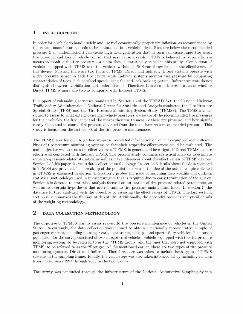
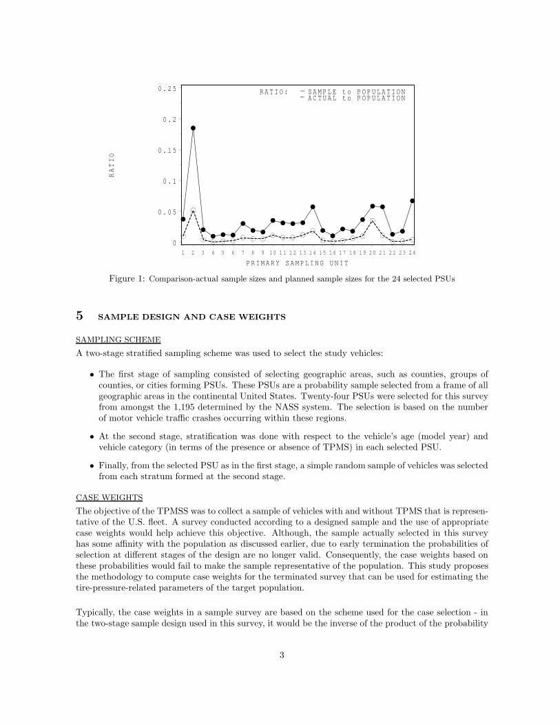
Given the reduced sample size, it was of interest in this study to assess how well the actual samplecould represent the population. This is done by comparing the ratio, Rplanned of planned sample sizeto the corresponding PSU size with the ratio Ractual of actual sample size to the corresponding PSUsize. Figure 1 presents profiles of these two ratios over PSUs in which data were collected. The patternsof the two ratios in this figure shows that the number of vehicles actually documented in the sample isconsistently proportional to the planned PSU sample sizes. However, this does not completely make thesample nationally representative in certain other aspects of the sample design. Therefore, an adjustmentneeds to be made through case weights to achieve a reasonable level of national representation. Thefollowing section is devoted to developing these weights.

2

R A T I O : S A M P L E t o P O P U L A T I O N A C T U A L t o P O P U L A T I O N

RATIO

0

0 . 0 5

0 . 1

0 . 1 5

0 . 2

0 . 2 5

P R I M A R Y S A M P L I N G U N I T

1 2 3 4 5 6 7 8 9 1 0 1 1 1 2 1 3 1 4 1 5 1 6 1 7 1 8 1 9 2 0 2 1 2 2 2 3 2 4

Figure 1: Comparison-actual sample sizes and planned sample sizes for the 24 selected PSUs

5 SAMPLE DESIGN AND CASE WEIGHTS

SAMPLING SCHEME

A two-stage stratified sampling scheme was used to select the study vehicles:

• The first stage of sampling consisted of selecting geographic areas, such as counties, groups ofcounties, or cities forming PSUs. These PSUs are a probability sample selected from a frame of allgeographic areas in the continental United States. Twenty-four PSUs were selected for this surveyfrom amongst the 1,195 determined by the NASS system. The selection is based on the numberof motor vehicle traffic crashes occurring within these regions.

• At the second stage, stratification was done with respect to the vehicle’s age (model year) andvehicle category (in terms of the presence or absence of TPMS) in each selected PSU.

• Finally, from the selected PSU as in the first stage, a simple random sample of vehicles was selectedfrom each stratum formed at the second stage.

CASE WEIGHTS

The objective of the TPMSS was to collect a sample of vehicles with and without TPMS that is represen-tative of the U.S. fleet. A survey conducted according to a designed sample and the use of appropriatecase weights would help achieve this objective. Although, the sample actually selected in this surveyhas some affinity with the population as discussed earlier, due to early termination the probabilities ofselection at different stages of the design are no longer valid. Consequently, the case weights based onthese probabilities would fail to make the sample representative of the population. This study proposesthe methodology to compute case weights for the terminated survey that can be used for estimating thetire-pressure-related parameters of the target population.

Typically, the case weights in a sample survey are based on the scheme used for the case selection - inthe two-stage sample design used in this survey, it would be the inverse of the product of the probability

3

of PSU selection and the probability of vehicle selection from a stratum. Originally, the weight for theith case selected randomly form the jth stratum of the kth selected PSU was defined as

W oijk =

(

1

Pk

) (

1

Pij/k

)

, (1)

where Pk = Prob {kth PSU is selected }, Pij/k = Prob {ith vehicle is selected from jth stratum, given

that kth PSU has been selected}.

Although the survey was terminated prior to completion of data collection based on the laid-down sampledesign, the PSU selection had already been made. This preserves the probability Pk of PSU selection.However, due to early termination, the selection of vehicles in the strata was disturbed - fewer thanplanned vehicles could be selected in the strata. This questions the validity of the corresponding selec-tion probability Pij/k. To introduce a reasonable amount of national representation, revision of theseprobabilities is imperative. What is needed is to account for what was actually selected in a stratum asagainst what was supposed to be selected. This suggests that the posterior rather than the prior dis-tribution should be used for computing the vehicle selection probability Pij/k to be used in computingweights as in (1). Based on this rationale, this study proposes a Bayesian methodology to compute caseselection probabilities Pij/k, and hence the case weights Wijk.

Consider the sampling design layout for an exemplar PSU as shown in Table 2, where nij is the samplesize originally planned to be collected from the stratum (ij) of the PSU and mij is the sample sizeactually collected from the ijth stratum.

Table 2: Stratification in an exemplar PSU.

Vehicle Age Vehicle group

With TPMS Without TPMS

(Study group) (Peer group)

Less than 3 years n11 n12

(New vehicles) m11 m12

3 years or older n21 n22

(Old vehicles) m21 m22

The case selection at each stage is basically a Bernoulli process with probability of selection (success)determined by the ratio of the number to be selected to the number from which to be selected. Thus, ifin a stratum of Nij vehicles, nij are to be selected, then the probability of selection (success, speakingin terms of bernoulli trials), is the ratio (π = nij/Nij.) However, instead of nij vehicles, only mij

(mij ≤ nij) could be selected by the time the survey was terminated. Speaking in terms of the bernoullitrials, this amounts to having mij successes in nij trials with probability of success given by π. It is thisprobability that needs to be revised using the prior information about the sample size. Bayesian approachis used for this purpose as outlined in the appendix. The probability that maximizes the selection of ith

vehicle from the jth stratum of the kth PSU, that is the mode of the posterior distribution [1], is givenby

π∗ =(mij − 1/2)

(nij − 1)(2)

Finally, in the two-stage selection process used in the survey, the probability of selection of a vehicle isthe product of the probability of selection Pk of the kth PSU and the posterior probability given by (2),

4

that is

P ∗ijk = Pk ∗

(

mij − 1/2

nij − 1

)

. (3)

However, some adjustments are needed before this posterior probability of case selection could be usedin calculating case weights. It should be noted that the strata in which the number of vehicles actuallyselected is equal to the number that was originally planed for a stratum do not require the Bayesiantreatment. Thus, the case weights are calculated using the formula (1) or (3), depending upon whetherthe number of vehicles actually selected is equal to or less than the number of vehicles planned to beselected. Further, non-response in a survey is not uncommon. To account for this contingency, theweights need to be adjusted by using the response rates in the selected strata. Finally, the case selectionprobabilities and hence the case weights are calculated by

Wijk =

(

1Pk

) (

Nij

nij

)(

1rj

)

, if mij = nij

(

1Pk

) (

nij−1

mij−1

2

) (

1rj

)

, if mij < nij ,

where rj×100 (rj ≤ 1) percent is the response rate in the jth stratum.

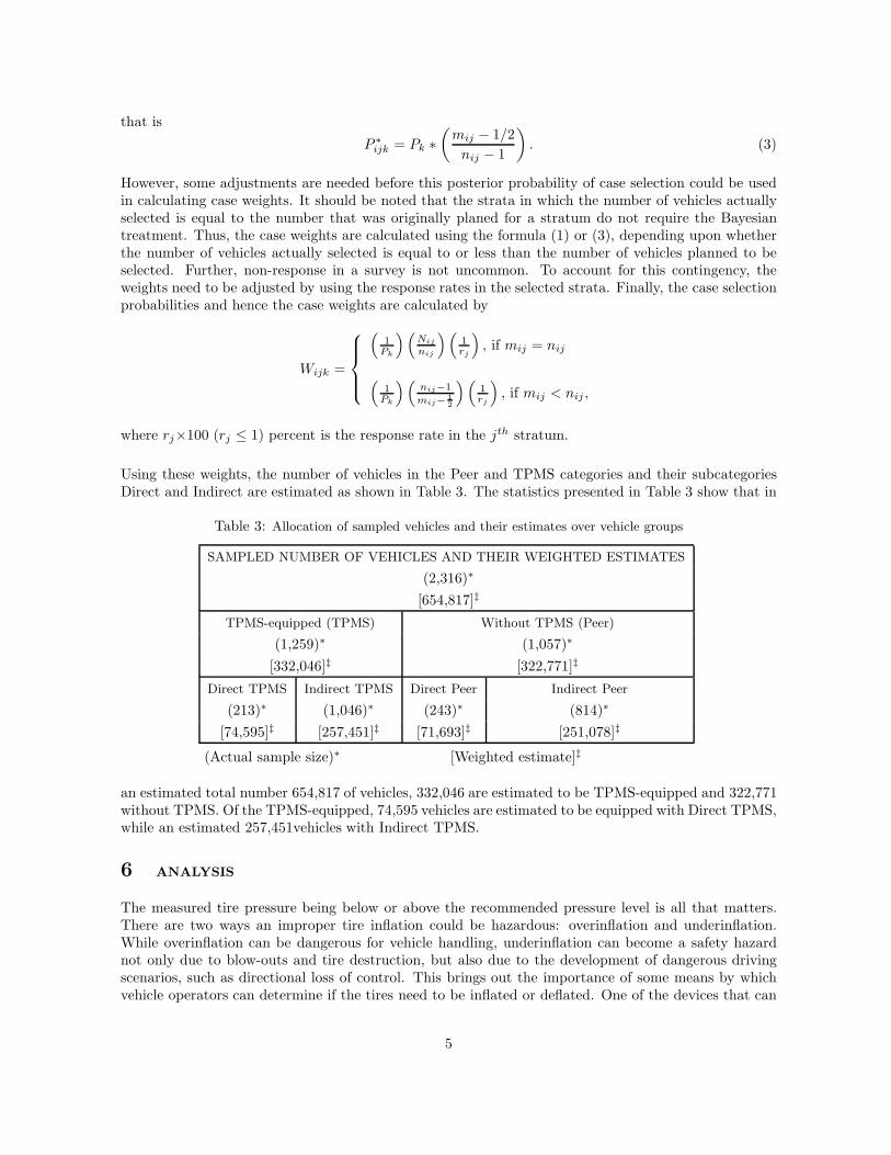
Using these weights, the number of vehicles in the Peer and TPMS categories and their subcategoriesDirect and Indirect are estimated as shown in Table 3. The statistics presented in Table 3 show that in

Table 3: Allocation of sampled vehicles and their estimates over vehicle groups

SAMPLED NUMBER OF VEHICLES AND THEIR WEIGHTED ESTIMATES

(2,316)∗

[654,817]‡

TPMS-equipped (TPMS)

(1,259)∗

[332,046]‡

Without TPMS (Peer)

(1,057)∗

[322,771]‡

Direct TPMS Indirect TPMS Direct Peer Indirect Peer

(213)∗

[74,595]‡(1,046)∗

[257,451]‡(243)∗

[71,693]‡(814)∗

[251,078]‡

(Actual sample size)∗ [Weighted estimate]‡

an estimated total number 654,817 of vehicles, 332,046 are estimated to be TPMS-equipped and 322,771without TPMS. Of the TPMS-equipped, 74,595 vehicles are estimated to be equipped with Direct TPMS,while an estimated 257,451vehicles with Indirect TPMS.

6 ANALYSIS

The measured tire pressure being below or above the recommended pressure level is all that matters.There are two ways an improper tire inflation could be hazardous: overinflation and underinflation.While overinflation can be dangerous for vehicle handling, underinflation can become a safety hazardnot only due to blow-outs and tire destruction, but also due to the development of dangerous drivingscenarios, such as directional loss of control. This brings out the importance of some means by whichvehicle operators can determine if the tires need to be inflated or deflated. One of the devices that can

5

be used for this purpose is TPMS. This study is focused on assessing the effectiveness of TPMS as ameans to maintain tire inflation at the recommend levels, as well as study the comparative effectivenessof Direct and Indirect TPMS. One of the ways this can be done is to compare the TPMS group ofvehicles with the Peer group and TPMS Direct subgroup with TPMS Indirect subgroup. This studymakes these comparisons in terms of the frequencies of underinflated and overinflated vehicles for thetwo groups, as well as their average underinflation and overinflation. Statistical analysis is conducted toestimate some tire-inflation-related parameters using the proposed weights and test certain hypothesesto compare groups of vehicles with and without TPMS, as well as their respective subgroups, Direct andIndirect.

The tire-pressure-related parameters that can be used to determine underinflation and overinflation arethe manufacturer’s recommended tire inflation pressure and the one actually measured in the survey foreach tire of a vehicle. The difference between the two is used to determine the extent of underinflationand overinflation of a tire:

• Underinflation = Recommended pressure - Measured pressure (≥ 0, recommended exceeds mea-sured)

• Overinflation = Measured pressure - Recommended pressure (≥ 0, measured exceeds recom-mended)

For the analysis purpose, these are converted into percentages (percentage of the corresponding recom-mended pressure of the subject tire) for each tire of the vehicle.

With regard to the tire pressure status of a vehicle on the whole, an underinflated vehicle in this studyrefers to a vehicle that has at least one tire underinflated. The same criterion is used in the case ofoverinflation. It should be noted that a vehicle can have both underinflated and overinflated tires.

While the variables Underinflation and Overinflation are computed for all the tires of a vehicle, theminimum of all tire pressures in the case of underinflation and maximum of all tire pressures in the caseof overinflation are used as measures of vehicle underinflation and overinflation, respectively.

6.1 Preliminary Analysis

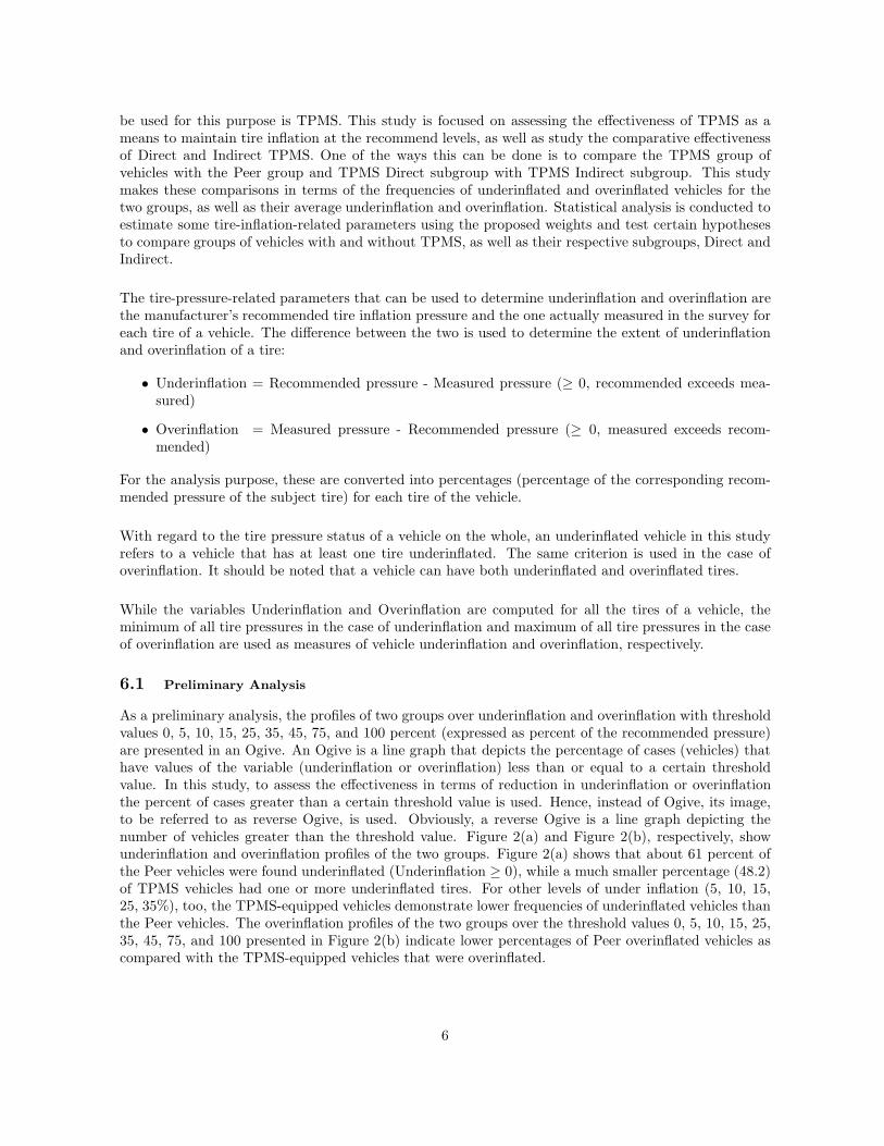
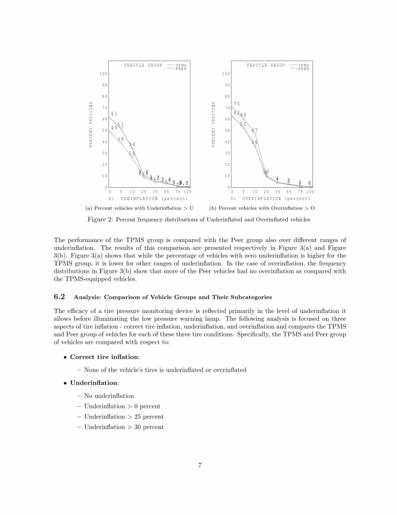
As a preliminary analysis, the profiles of two groups over underinflation and overinflation with thresholdvalues 0, 5, 10, 15, 25, 35, 45, 75, and 100 percent (expressed as percent of the recommended pressure)are presented in an Ogive. An Ogive is a line graph that depicts the percentage of cases (vehicles) thathave values of the variable (underinflation or overinflation) less than or equal to a certain thresholdvalue. In this study, to assess the effectiveness in terms of reduction in underinflation or overinflationthe percent of cases greater than a certain threshold value is used. Hence, instead of Ogive, its image,to be referred to as reverse Ogive, is used. Obviously, a reverse Ogive is a line graph depicting thenumber of vehicles greater than the threshold value. Figure 2(a) and Figure 2(b), respectively, showunderinflation and overinflation profiles of the two groups. Figure 2(a) shows that about 61 percent ofthe Peer vehicles were found underinflated (Underinflation ≥ 0), while a much smaller percentage (48.2)of TPMS vehicles had one or more underinflated tires. For other levels of under inflation (5, 10, 15,25, 35%), too, the TPMS-equipped vehicles demonstrate lower frequencies of underinflated vehicles thanthe Peer vehicles. The overinflation profiles of the two groups over the threshold values 0, 5, 10, 15, 25,35, 45, 75, and 100 presented in Figure 2(b) indicate lower percentages of Peer overinflated vehicles ascompared with the TPMS-equipped vehicles that were overinflated.

6

U : U D E I N F L A T I O N ( p e r c e n t )

V E H IC LE G RO UP TPMSPEER

PERCENT VEHICLES

0

1 0

2 0

3 0

40

50

60

70

80

90

100

0 5 10 25 35 45 75 100

4 9

3 9

2 6

8 . 44 . 2 2 . 6 0 . 60 . 0

6 1

5 1

3 4

9 . 95 . 4 3 . 4

0 . 30 . 0

O: OVER INFLA TION (pe rcent )

VE HICLE GRO UP TPMSPEER

PERCENT VEHICLES

0

1 0

2 0

3 0

40

50

60

70

80

90

100

0 5 10 25 35 45 75 100

7 0

6 0

4 7

1 0

4 2 0 0

6 2

5 2

3 6

94 3 1 0

(a) Percent vehicles with Underinflation > U (b) Percent vehicles with Overinflation > O

Figure 2: Percent frequency distributions of Underinflated and Overinflated vehicles

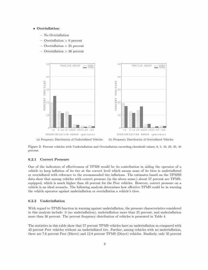
The performance of the TPMS group is compared with the Peer group also over different ranges ofunderinflation. The results of this comparison are presented respectively in Figure 3(a) and Figure3(b). Figure 3(a) shows that while the percentage of vehicles with zero underinflation is higher for theTPMS group, it is lower for other ranges of underinflation. In the case of overinflation, the frequencydistributions in Figure 3(b) show that more of the Peer vehicles had no overinflation as compared withthe TPMS-equipped vehicles.

6.2 Analysis: Comparison of Vehicle Groups and Their Subcategories

The efficacy of a tire pressure monitoring device is reflected primarily in the level of underinflation itallows before illuminating the low pressure warning lamp. The following analysis is focused on threeaspects of tire inflation - correct tire inflation, underinflation, and overinflation and compares the TPMSand Peer group of vehicles for each of these three tire conditions. Specifically, the TPMS and Peer groupof vehicles are compared with respect to:

• Correct tire inflation:

– None of the vehicle’s tires is underinflated or overinflated

• Underinflation:

– No underinflation

– Underinflation > 0 percent



7

• Overinflation:

– No Overinflation

– Overinflation > 0 percent



U N D E R I N F L A T I O N R A N G E ( p e r c e n t )

VE H I CL E GR OU P PEERTPMS

PERCENT VEHICLES

0

1 0

2 0

3 0

4 0

5 0

= 0 0 -1 0 1 0- 252 5 - 353 5- 4 5 >45

OVERINFLATION RANGE (percent)

VEH ICLE GROU P PEERTPMS

PERCENT VEHICLES

0

10

20

30

40

50

=0 0 -10 1 0-2525 -3535-4 5 >45

(a) Frequency Distribution of Underinflated Vehicles (b) Frequency Distribution of Overinflated Vehicles

Figure 3: Percent vehicles with Underinflation and Overinflation exceeding threshold values, 0, 5, 10, 25, 35, 45percent.

6.2.1 Correct Pressure

One of the indicators of effectiveness of TPMS would be its contribution in aiding the operator of avehicle to keep inflation of its tire at the correct level which means none of its tires is underinflatedor overinflated with reference to the recommended tire inflations. The estimates based on the TPMSSdata show that among vehicles with correct pressure (in the above sense,) about 57 percent are TPMS-equipped, which is much higher than 43 percent for the Peer vehicles. However, correct pressure on avehicle is an ideal scenario. The following analysis determines how effective TPMS could be in warningthe vehicle operator against underinflation or overinflation a vehicle’s tires.

6.2.2 Underinflation

With regard to TPMS function in warning against underinflation, the pressure characteristics consideredin this analysis include: 0 (no underinflation), underinflation more than 25 percent, and underinflationmore than 30 percent. The percent frequency distribution of vehicles is presented in Table 4.

The statistics in this table show that 57 percent TPMS vehicles have no underinflation as compared with43 percent Peer vehicles without an underinflated tire. Further, among vehicles with no underinflation,there are 7.6 percent Peer (Direct) and 12.8 percent TPMS (Direct) vehicles. Similarly, only 35 percent

8

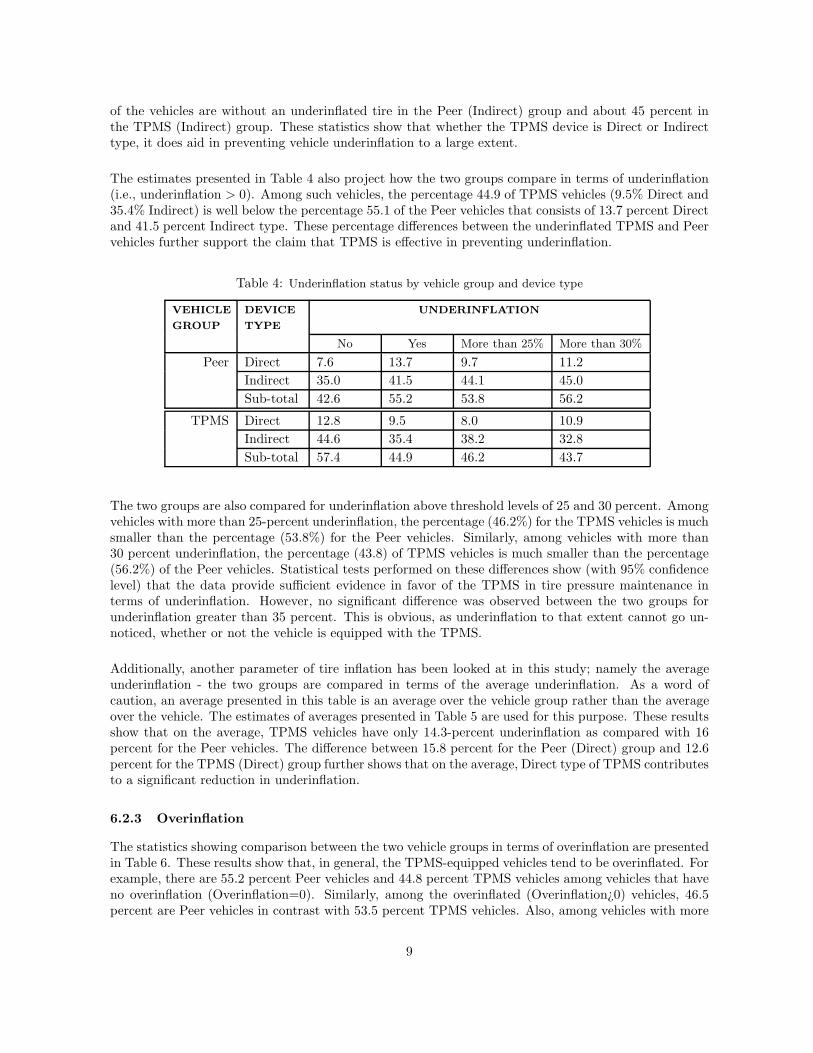
of the vehicles are without an underinflated tire in the Peer (Indirect) group and about 45 percent inthe TPMS (Indirect) group. These statistics show that whether the TPMS device is Direct or Indirecttype, it does aid in preventing vehicle underinflation to a large extent.

The estimates presented in Table 4 also project how the two groups compare in terms of underinflation(i.e., underinflation > 0). Among such vehicles, the percentage 44.9 of TPMS vehicles (9.5% Direct and35.4% Indirect) is well below the percentage 55.1 of the Peer vehicles that consists of 13.7 percent Directand 41.5 percent Indirect type. These percentage differences between the underinflated TPMS and Peervehicles further support the claim that TPMS is effective in preventing underinflation.

Table 4: Underinflation status by vehicle group and device type

VEHICLE DEVICE UNDERINFLATION

GROUP TYPE

No Yes More than 25% More than 30%

Peer Direct 7.6 13.7 9.7 11.2

Indirect 35.0 41.5 44.1 45.0

Sub-total 42.6 55.2 53.8 56.2

TPMS Direct 12.8 9.5 8.0 10.9

Indirect 44.6 35.4 38.2 32.8

Sub-total 57.4 44.9 46.2 43.7

The two groups are also compared for underinflation above threshold levels of 25 and 30 percent. Amongvehicles with more than 25-percent underinflation, the percentage (46.2%) for the TPMS vehicles is muchsmaller than the percentage (53.8%) for the Peer vehicles. Similarly, among vehicles with more than30 percent underinflation, the percentage (43.8) of TPMS vehicles is much smaller than the percentage(56.2%) of the Peer vehicles. Statistical tests performed on these differences show (with 95% confidencelevel) that the data provide sufficient evidence in favor of the TPMS in tire pressure maintenance interms of underinflation. However, no significant difference was observed between the two groups forunderinflation greater than 35 percent. This is obvious, as underinflation to that extent cannot go un-noticed, whether or not the vehicle is equipped with the TPMS.

Additionally, another parameter of tire inflation has been looked at in this study; namely the averageunderinflation - the two groups are compared in terms of the average underinflation. As a word ofcaution, an average presented in this table is an average over the vehicle group rather than the averageover the vehicle. The estimates of averages presented in Table 5 are used for this purpose. These resultsshow that on the average, TPMS vehicles have only 14.3-percent underinflation as compared with 16percent for the Peer vehicles. The difference between 15.8 percent for the Peer (Direct) group and 12.6percent for the TPMS (Direct) group further shows that on the average, Direct type of TPMS contributesto a significant reduction in underinflation.

6.2.3 Overinflation

The statistics showing comparison between the two vehicle groups in terms of overinflation are presentedin Table 6. These results show that, in general, the TPMS-equipped vehicles tend to be overinflated. Forexample, there are 55.2 percent Peer vehicles and 44.8 percent TPMS vehicles among vehicles that haveno overinflation (Overinflation=0). Similarly, among the overinflated (Overinflation¿0) vehicles, 46.5percent are Peer vehicles in contrast with 53.5 percent TPMS vehicles. Also, among vehicles with more

9


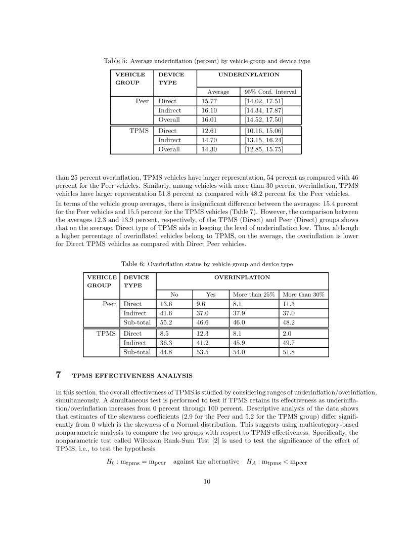
Table 5: Average underinflation (percent) by vehicle group and device type

VEHICLE DEVICE UNDERINFLATION

GROUP TYPE

Peer Direct

Indirect

Overall

Average

15.77

16.10

16.01

95% Conf. Interval

[14.02, 17.51]

[14.34, 17.87]

[14.52, 17.50]

TPMS Direct

Indirect

Overall

12.61

14.70

14.30

[10.16, 15.06]

[13.15, 16.24]

[12.85, 15.75]

than 25 percent overinflation, TPMS vehicles have larger representation, 54 percent as compared with 46percent for the Peer vehicles. Similarly, among vehicles with more than 30 percent overinflation, TPMSvehicles have larger representation 51.8 percent as compared with 48.2 percent for the Peer vehicles.

In terms of the vehicle group averages, there is insignificant difference between the averages: 15.4 percentfor the Peer vehicles and 15.5 percent for the TPMS vehicles (Table 7). However, the comparison betweenthe averages 12.3 and 13.9 percent, respectively, of the TPMS (Direct) and Peer (Direct) groups showsthat on the average, Direct type of TPMS aids in keeping the level of underinflation low. Thus, althougha higher percentage of overinflated vehicles belong to TPMS, on the average, the overinflation is lowerfor Direct TPMS vehicles as compared with Direct Peer vehicles.

Table 6: Overinflation status by vehicle group and device type

VEHICLE DEVICE OVERINFLATION

GROUP TYPE

No Yes More than 25% More than 30%

Peer Direct 13.6 9.6 8.1 11.3

Indirect 41.6 37.0 37.9 37.0

Sub-total 55.2 46.6 46.0 48.2

TPMS Direct 8.5 12.3 8.1 2.0

Indirect 36.3 41.2 45.9 49.7

Sub-total 44.8 53.5 54.0 51.8

7 TPMS EFFECTIVENESS ANALYSIS

In this section, the overall effectiveness of TPMS is studied by considering ranges of underinflation/overinflation,simultaneously. A simultaneous test is performed to test if TPMS retains its effectiveness as underinfla-tion/overinflation increases from 0 percent through 100 percent. Descriptive analysis of the data showsthat estimates of the skewness coefficients (2.9 for the Peer and 5.2 for the TPMS group) differ signifi-cantly from 0 which is the skewness of a Normal distribution. This suggests using multicategory-basednonparametric analysis to compare the two groups with respect to TPMS effectiveness. Specifically, thenonparametric test called Wilcoxon Rank-Sum Test [2] is used to test the significance of the effect ofTPMS, i.e., to test the hypothesis

H0 : mtpms = mpeer against the alternative HA : mtpms < mpeer

10

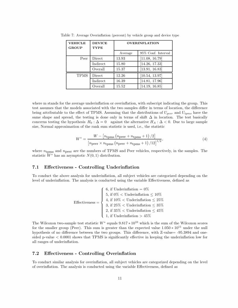
Table 7: Average Overinflation (percent) by vehicle group and device type

VEHICLE DEVICE OVERINFLATION

GROUP TYPE

Peer Direct

Indirect

Overall

Average

13.93

15.80

15.37

95% Conf. Interval

[11.08, 16.79]

[14.26, 17.33]

[13.91, 16.83]

TPMS Direct

Indirect

Overall

12.26

16.39

15.52

[10.54, 13.97]

[14.81, 17.96]

[14.19, 16.85]

where m stands for the average underinflation or overinflation, with subscript indicating the group. Thistest assumes that the models associated with the two samples differ in terms of location, the differencebeing attributable to the effect of TPMS. Assuming that the distributions of Upeer and Utpms have thesame shape and spread, the testing is done only in terms of shift ∆ in location. The test basicallyconcerns testing the hypothesis H0 : ∆ = 0 against the alternative HA : ∆ < 0. Due to large samplesize, Normal approximation of the rank sum statistic is used, i.e., the statistic

W ∗ =W −

[

ntpms(

npeer + ntpms + 1)

/2]

npeer × ntpms npeer + ntpms + 1 /121/2

, (4)[ ( ) ]

where ntpms and npeer are the numbers of TPMS and Peer vehicles, respectively, in the samples. Thestatistic W ∗ has an asymptotic N(0, 1) distribution.

7.1 Effectiveness - Controlling Underinflation

To conduct the above analysis for underinflation, all subject vehicles are categorized depending on thelevel of underinflation. The analysis is conducted using the variable Effectiveness, defined as

6, if Underinflation = 0%

5, if 0% < Underinflation ≤ 10%

4, if 10% < Underinflation ≤ 25%Effectiveness =



1, if Underinflation > 45%

The Wilcoxon two-sample test statistic W

∗ equals 9.817 ∗ 1010 which is the sum of the Wilcoxon scoresfor the smaller group (Peer). This sum is greater than the expected value 1.050 ∗ 1011 under the nullhypothesis of no difference between the two groups. This difference, with Z-value= -95.3894 and one-sided p-value < 0.0001 shows that TPMS is significantly effective in keeping the underinflation low forall ranges of underinflation.

7.2 Effectiveness - Controlling Overinflation

To conduct similar analysis for overinflation, all subject vehicles are categorized depending on the levelof overinflation. The analysis is conducted using the variable Effectiveness, defined as

11

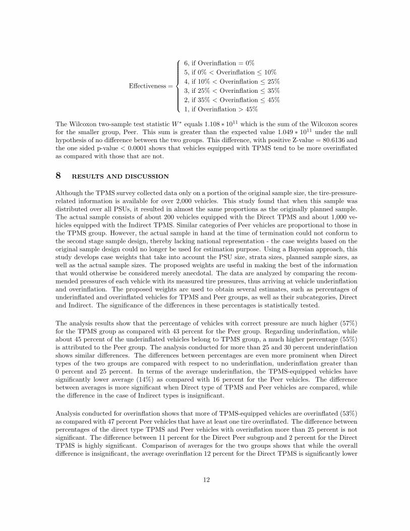
6, if Overinflation = 0%

5, if 0% < Overinflation ≤ 10%

4, if 10% < Overinflation ≤ 25%Effectiveness =



1, if Overinflation > 45%

The Wilcoxon two-sample test statistic W ∗ equals 1.108 ∗ 1011 which is the sum of the Wilcoxon scoresfor the smaller group, Peer. This sum is greater than the expected value 1.049 ∗ 1011 under the nullhypothesis of no difference between the two groups. This difference, with positive Z-value = 80.6136 andthe one sided p-value < 0.0001 shows that vehicles equipped with TPMS tend to be more overinflatedas compared with those that are not.

8 RESULTS AND DISCUSSION

Although the TPMS survey collected data only on a portion of the original sample size, the tire-pressure-related information is available for over 2,000 vehicles. This study found that when this sample wasdistributed over all PSUs, it resulted in almost the same proportions as the originally planned sample.The actual sample consists of about 200 vehicles equipped with the Direct TPMS and about 1,000 ve-hicles equipped with the Indirect TPMS. Similar categories of Peer vehicles are proportional to those inthe TPMS group. However, the actual sample in hand at the time of termination could not conform tothe second stage sample design, thereby lacking national representation - the case weights based on theoriginal sample design could no longer be used for estimation purpose. Using a Bayesian approach, thisstudy develops case weights that take into account the PSU size, strata sizes, planned sample sizes, aswell as the actual sample sizes. The proposed weights are useful in making the best of the informationthat would otherwise be considered merely anecdotal. The data are analyzed by comparing the recom-mended pressures of each vehicle with its measured tire pressures, thus arriving at vehicle underinflationand overinflation. The proposed weights are used to obtain several estimates, such as percentages ofunderinflated and overinflated vehicles for TPMS and Peer groups, as well as their subcategories, Directand Indirect. The significance of the differences in these percentages is statistically tested.

The analysis results show that the percentage of vehicles with correct pressure are much higher (57%)for the TPMS group as compared with 43 percent for the Peer group. Regarding underinflation, whileabout 45 percent of the underinflated vehicles belong to TPMS group, a much higher percentage (55%)is attributed to the Peer group. The analysis conducted for more than 25 and 30 percent underinflationshows similar differences. The differences between percentages are even more prominent when Directtypes of the two groups are compared with respect to no underinflation, underinflation greater than0 percent and 25 percent. In terms of the average underinflation, the TPMS-equipped vehicles havesignificantly lower average (14%) as compared with 16 percent for the Peer vehicles. The differencebetween averages is more significant when Direct type of TPMS and Peer vehicles are compared, whilethe difference in the case of Indirect types is insignificant.

Analysis conducted for overinflation shows that more of TPMS-equipped vehicles are overinflated (53%)as compared with 47 percent Peer vehicles that have at least one tire overinflated. The difference betweenpercentages of the direct type TPMS and Peer vehicles with overinflation more than 25 percent is notsignificant. The difference between 11 percent for the Direct Peer subgroup and 2 percent for the DirectTPMS is highly significant. Comparison of averages for the two groups shows that while the overalldifference is insignificant, the average overinflation 12 percent for the Direct TPMS is significantly lower

12

than 14 percent for the Direct Peer vehicles.

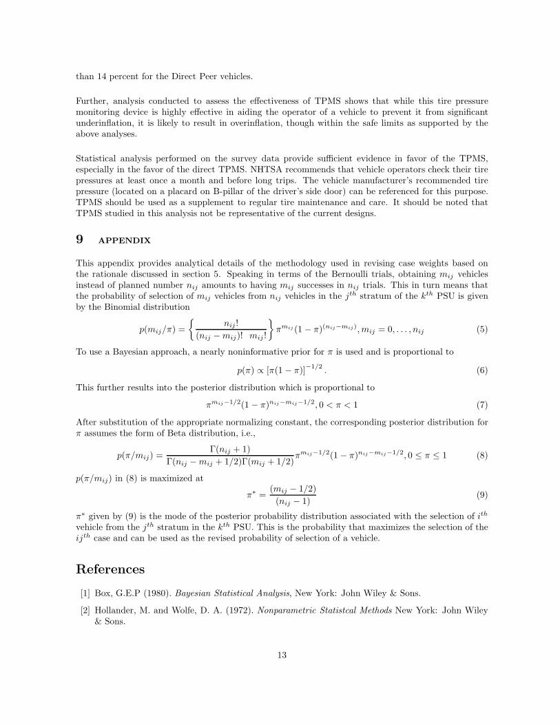
Further, analysis conducted to assess the effectiveness of TPMS shows that while this tire pressuremonitoring device is highly effective in aiding the operator of a vehicle to prevent it from significantunderinflation, it is likely to result in overinflation, though within the safe limits as supported by theabove analyses.

Statistical analysis performed on the survey data provide sufficient evidence in favor of the TPMS,especially in the favor of the direct TPMS. NHTSA recommends that vehicle operators check their tirepressures at least once a month and before long trips. The vehicle manufacturer’s recommended tirepressure (located on a placard on B-pillar of the driver’s side door) can be referenced for this purpose.TPMS should be used as a supplement to regular tire maintenance and care. It should be noted thatTPMS studied in this analysis not be representative of the current designs.

9 APPENDIX

This appendix provides analytical details of the methodology used in revising case weights based onthe rationale discussed in section 5. Speaking in terms of the Bernoulli trials, obtaining mij vehiclesinstead of planned number nij amounts to having mij successes in nij trials. This in turn means thatthe probability of selection of mij vehicles from n vehicles in the jth stratum of the kth

ij PSU is givenby the Binomial distribution

p(mij/π) =

{

nij !

(nij − mij)! mij !

}

πmij (1 − π)(nij−mij), mij = 0, . . . , nij (5)

To use a Bayesian approach, a nearly noninformative prior for π is used and is proportional to

p(π) ∝ [π(1 − π)]−1/2

. (6)

This further results into the posterior distribution which is proportional to

πmij−1/2(1 − π)nij−mij−1/2, 0 < π < 1 (7)

After substitution of the appropriate normalizing constant, the corresponding posterior distribution forπ assumes the form of Beta distribution, i.e.,

p(π/mij) =Γ(nij + 1)

Γ(nij − mij + 1/2)Γ(mij + 1/2)πmij−1/2(1 − π)nij−mij−1/2, 0 ≤ π ≤ 1 (8)

p(π/mij) in (8) is maximized at

π∗ =(mij − 1/2)

(nij − 1)(9)

π∗ given by (9) is the mode of the posterior probability distribution associated with the selection of ith

vehicle from the jth stratum in the kth PSU. This is the probability that maximizes the selection of theijth case and can be used as the revised probability of selection of a vehicle.

References

[1] Box, G.E.P (1980). Bayesian Statistical Analysis, New York: John Wiley & Sons.

[2] Hollander, M. and Wolfe, D. A. (1972). Nonparametric Statistcal Methods New York: John Wiley& Sons.

13

DOT HS 811 086April 2009

Documents

Tire Pressure Maintenance - A Statistical Investigation