Embed Size (px)
Citation preview

Timing-Driven Macro Placement
Dissertation
zur
Erlangung des Doktorgrades (Dr. rer. nat.)
der
Mathematisch-Naturwissenschaftlichen Fakultät
der
Rheinischen Friedrich-Wilhelms-Universität Bonn
Vorgelegt von
Philipp Ochsendorf
geboren in
Frankfurt am Main
Bonn, Januar 2019

Angefertigt mit Genehmigung der Mathematisch-Naturwissenschaftlichen Fakultät derRheinischen Friedrich-Wilhelms-Universität Bonn
Erstgutachter: Herr Professor Dr. Jens VygenZweitgutachter: Herr Professor Dr. Dr. h.c. Bernhard Korte
Tag der Promotion: 22. März 2019Erscheinungsjahr: 2019
ii

Acknowledgments
This dissertation would not have been possible without the support of many people. Firstand foremost I would like to express my gratitude to Professor Dr. Jens Vygen for theinspiring supervision of my doctoral studies.
I also wish to thank Professor Dr. Dr. h.c. Bernhard Korte and Professor Dr. StefanHougardy for providing outstanding working conditions at the Research Institute forDiscrete Mathematics of the University of Bonn.
I would also like to thank the present and past members of the BonnPlace-Team,especially Dr. Ulrich Brenner, Dr. Jan Schneider and Jannik Silvanus. The extremely goodatmosphere in this team, the support as well as the fruitful discussions and ideas provedto be invaluable. Special thanks also go to all students for their collaboration, especiallyNils Hoppmann.
I also thank all other colleagues of the institute for inspiring discussions, in particularAnna Hermann. Special thanks go to Professor Dr. Stephan Held for his support with theIBM timing environment. Furthermore I thank Dr. Christoph Bartoschek for his influenceon my programming attitude, which set me off on the right track.
But my biggest thanks go to Conni, my parents and my sister Lisa. Without theirpermanent support, encouragement and endless patience, I would not have been able tofinish this thesis.
iii


Contents
Acknowledgments iii
Contents v
1 Introduction 1
2 Placement Problems 32.1 Basic Definitions . . . . . . . . . . . . . . . . . . . . . . . . . . . . . . . . . 32.2 Placement . . . . . . . . . . . . . . . . . . . . . . . . . . . . . . . . . . . . . 4
2.2.1 Placement Constraints . . . . . . . . . . . . . . . . . . . . . . . . . . 52.2.2 Placement Objectives . . . . . . . . . . . . . . . . . . . . . . . . . . 72.2.3 Placement Problem Variants . . . . . . . . . . . . . . . . . . . . . . 10
2.3 Macro Placement . . . . . . . . . . . . . . . . . . . . . . . . . . . . . . . . . 112.4 Standard Cell Placement . . . . . . . . . . . . . . . . . . . . . . . . . . . . . 14
3 Timing-Driven Rectangle Packing 193.1 Distance-Bound Model . . . . . . . . . . . . . . . . . . . . . . . . . . . . . . 193.2 Computing Distance-Bounds . . . . . . . . . . . . . . . . . . . . . . . . . . 253.3 Basic Properties . . . . . . . . . . . . . . . . . . . . . . . . . . . . . . . . . 273.4 Strongly Polynomial Algorithm . . . . . . . . . . . . . . . . . . . . . . . . . 313.5 Distance Bound Pruning . . . . . . . . . . . . . . . . . . . . . . . . . . . . . 393.6 LP-Formulation for Fixed Relations . . . . . . . . . . . . . . . . . . . . . . 43
4 Timing-Driven Macro Placement 474.1 Shredded Placement . . . . . . . . . . . . . . . . . . . . . . . . . . . . . . . 48
4.1.1 Placement with Shredded Macros . . . . . . . . . . . . . . . . . . . . 494.1.2 Macro Reassembly . . . . . . . . . . . . . . . . . . . . . . . . . . . . 50
4.2 Macro Legalization . . . . . . . . . . . . . . . . . . . . . . . . . . . . . . . . 504.2.1 Macro Packing . . . . . . . . . . . . . . . . . . . . . . . . . . . . . . 524.2.2 Choosing Unconstrained Rectangles . . . . . . . . . . . . . . . . . . 544.2.3 Selecting the Window . . . . . . . . . . . . . . . . . . . . . . . . . . 554.2.4 Computing Feasible Areas . . . . . . . . . . . . . . . . . . . . . . . . 574.2.5 Choosing Spatial Relations . . . . . . . . . . . . . . . . . . . . . . . 574.2.6 Solving the Rectangle Packing Problem . . . . . . . . . . . . . 584.2.7 Local Post-Optimization . . . . . . . . . . . . . . . . . . . . . . . . . 59
4.3 Timing-Driven Macro Legalization . . . . . . . . . . . . . . . . . . . . . . . 604.3.1 Distance Bound Construction . . . . . . . . . . . . . . . . . . . . . . 604.3.2 Timing-Driven Macro Packing . . . . . . . . . . . . . . . . . . . . . 61
v

Contents
4.3.3 Solving the Timing-Driven Rectangle Packing Problem . . . 624.3.4 Timing-Driven Local Post-Optimization . . . . . . . . . . . . . . . . 72
4.4 Post-Optimization . . . . . . . . . . . . . . . . . . . . . . . . . . . . . . . . 72
5 Global Placement 755.1 Fast Partitioning . . . . . . . . . . . . . . . . . . . . . . . . . . . . . . . . . 75
5.1.1 Movebound Constraints in Partitioning . . . . . . . . . . . . . . . . 765.1.2 Weak Movebound Homogeneity . . . . . . . . . . . . . . . . . . . . . 805.1.3 Weakly Movebound Homogeneous Regions . . . . . . . . . . . . . . 84
5.2 Self-Stabilizing BonnPlace . . . . . . . . . . . . . . . . . . . . . . . . . 885.2.1 General Framework . . . . . . . . . . . . . . . . . . . . . . . . . . . 885.2.2 Forces . . . . . . . . . . . . . . . . . . . . . . . . . . . . . . . . . . . 905.2.3 Breaking Conditions . . . . . . . . . . . . . . . . . . . . . . . . . . . 91
5.3 Routability-Driven Placement . . . . . . . . . . . . . . . . . . . . . . . . . . 915.3.1 Congestion Estimation . . . . . . . . . . . . . . . . . . . . . . . . . . 925.3.2 Density Adjustments . . . . . . . . . . . . . . . . . . . . . . . . . . . 93
5.4 Timing-Aware Placement . . . . . . . . . . . . . . . . . . . . . . . . . . . . 94
6 Experimental Results 976.1 Test Environment . . . . . . . . . . . . . . . . . . . . . . . . . . . . . . . . . 976.2 Partitioning with Movebounds . . . . . . . . . . . . . . . . . . . . . . . . . 996.3 Self-Stabilizing Behavior . . . . . . . . . . . . . . . . . . . . . . . . . . . . . 1026.4 Congestion-Driven Standard Cell Placement . . . . . . . . . . . . . . . . . . 103
6.4.1 Industrial Designs . . . . . . . . . . . . . . . . . . . . . . . . . . . . 1046.4.2 DAC 2012 Placement Contest . . . . . . . . . . . . . . . . . . . . . . 106
6.5 Timing-Driven Standard Cell Placement . . . . . . . . . . . . . . . . . . . . 1076.6 Mixed-Size Placement . . . . . . . . . . . . . . . . . . . . . . . . . . . . . . 111
6.6.1 Timing Results . . . . . . . . . . . . . . . . . . . . . . . . . . . . . . 1116.6.2 Running Time . . . . . . . . . . . . . . . . . . . . . . . . . . . . . . 1156.6.3 Outlook . . . . . . . . . . . . . . . . . . . . . . . . . . . . . . . . . . 119
Summary 121
Bibliography 123
Index 133
Notation 137
vi

Chapter 1
Introduction
Computer chips are at the heart of most electronic devices in our daily lives: embeddedsystems, smartphones, personal computers and servers. Many applications need powerfulchips that yet can be operated efficiently. At the same time processing ever increasingamounts of data constantly requires faster and faster microprocessors.
Creating the next generations of these miniature and almost magic devices is achievedin the physical design process. Here the most advanced manufacturing technologies meetwith the fields of computer science and mathematics. Many practical challenges can beformulated as fascinating combinatorial optimization problems.
Designing chips with billions of transistors would not be possible without the help ofautomatic tools. To manage this complexity, transistors are partitioned into modules thateither compute a Boolean function or store bits. These essential building blocks are calledcircuits or cells.
This thesis focuses on the placement problem, where circuits have to be arrangedwithout overlaps on the chip image. As one of the very first stages of physical design,placement quality has far reaching effects on the overall chip performance. At the sametime this stage is repeated frequently which particularly requires fast algorithms.
Favorable placements primarily need to enable good interconnections of the cells. Onthe one hand, these connections must be realized by wires in the subsequent routing designphase. On the other hand, all signals on a chip have to meet individual deadlines at whichthey must reach certain points on the design. Meeting these deadlines particularly requiresshort and thus fast connections. The deadlines define the contracts by which different cellsare guaranteed to interoperate correctly. Especially for modern technology nodes thesetiming challenges require great attention already during the placement stage.
Algorithms for placement usually distinguish between two types of problems: Macroplacement deals with comparably few but very large cells, the macros. Finding goodpositions for macros is challenging since packing macros disjointly is NP-hard and sincethe effect of macro positions on the overall placement objectives is hard to estimate. Withfixed macro positions the remainder of cells, the standard cells, all share a common width orheight. This property considerably simplifies finding feasible placements. But identifyinggood standard cell positions that can be routed easily and satisfy timing requirementsremains challenging, both in theory and practice.
To the best of our knowledge, we address timing characteristics for the very firsttime directly during macro placement. This leads to new extensions of BonnPlace,the placement framework of the BonnTools suite (Korte, Rautenbach and Vygen 2007)
1

Chapter 1. Introduction
developed at the Research Institute for Discrete Mathematics of the University of Bonnin an industrial cooperation with International Business Machines Corporation (IBM).
For this purpose we propose a new timing model for macros and develop algorithmsthat compute macro placements with good timing traits in this model. For evaluatingmacro placements thoroughly we extend BonnPlace to become more efficient and yetmore effective with respect to routing and timing objectives.
In Chapter 2 we formally introduce common chip design notation and outline generalplacement objectives and constraints, particularly arising from routing and timing opti-mization. Afterwards we focus on the two central problem variants, Macro Placementand Global Placement, before we review previous work.
Thereafter we explain how timing objectives for macros can be translated into geo-metric distance bounds. This leads to an extension of the classical Rectangle PackingProblem that is presented in Chapter 3. We analyze basic properties of this generalizedpacking problem before we develop a very efficient algorithm for a certain class of in-stances. We show in Theorem 3.34 that such instances can be solved optimally in O(nm)running time where n and m denote the number of rectangles and distance constraints.Moreover we devise strategies for computing equivalent and compact representations ofour macro timing model. We prove that for any pair of rectangles a single (generalized)distance constraint suffices.
Chapter 4 is devoted to BonnMacro, the macro placement module of BonnPlace.We first revisit the central approach of this algorithm. Afterwards we elaborate how tooptimize timing characteristics of macros in this framework. Therefore we develop theessential ingredient to enable this optimization: an efficient formulation as mixed-integerprogram.
In Chapter 5 we focus on global placement in order to evaluate timing characteristicsof macro placements accurately. We develop a geometric pre-processing to significantlyspeed up partitioning during BonnPlaceGlobal, the global placement module of Bonn-Place. The proposed model of partitioning as minimum-cost flow instance is proven tohave minimum cardinality. Furthermore we propose Self-Stabilizing BonnPlace, anextension of this partitioning-based placer by a force-directed placement framework. Thisapproach provides the necessary versatility for optimizing routing and timing objectivesat the same time.
The quality and performance of all presented algorithms is analyzed and discussedin Chapter 6, both on benchmark instances and on challenging real-world designs pro-vided by our industry partner IBM. We demonstrate the increased efficiency of par-titioning, particularly for the largest and most complicated test cases. The quality ofSelf-Stabilizing BonnPlace is confirmed both for congestion mitigation and timingoptimization on challenging designs. Thereafter we analyze our mixed-size placement flowthat combines timing-driven BonnMacro as well as Self-Stabilizing BonnPlace.
2

Chapter 2
Placement Problems
Placement is one of the most challenging and at the same time important steps in thephysical design of VLSI chips. The quality of the placement has far-reaching effects onthe whole design process.
In this chapter we elaborate the context of placement. We start by fixing a commonnotation in Section 2.1. Section 2.2 is devoted to introduce chip design notation andplacement problems in particular constraints (Section 2.2.1) and objectives (Section 2.2.2).Finally we introduce the two placement problems which are most important for this thesis:Macro Placement (Section 2.3) and Global Placement (Section 2.4). We explainfurther details and review previous work.
2.1 Basic DefinitionsThis thesis deals with a multitude of objects representable by rectangles. In order toestablish a common understanding, we fix the following notation:
Definition 2.1. A rectangle r ⊆ R2 is a set of the form r = [x0, x1 ] × [y0, y1 ] wherexi, yi ∈ R for i ∈ J2K and z0 < z1 for z ∈ x, y.
We emphasize that by Definition 2.1 rectangles are always closed, axis-parallel, non-empty and have non-zero area.
We mostly deal with configurations of rectangles with fixed width and height:
Definition 2.2. The (anchor) position of a rectangle r = [x0, x1 ]×[y0, y1 ] is the lower leftcorner (x0, y0) ∈ R2. Conversely placing r at p ∈ R2 means translating r by p− (x0, y0).
Note that by Definition 2.2 placing rectangle r at p ∈ R2 refers to the (anchor) positionof r. Thus clearly the position of r placed at p is p itself.
For shapes possibly composed of multiple rectangles, we use the following terminology:
Definition 2.3. A rectilinear shape is a set of points S ⊆ R2 for which k ∈ N andrectangles ri ⊆ R2 for i ∈ JkK exist with ⋃i∈JkK ri = S. The set of rectangles ri : i ∈ JkKis called a representation of S.
Clearly the representation of rectilinear shapes is not unique.
Definition 2.4. The intersection of rectangles a and b is a∩ b := (a ∩ b). Furthermorewe define the intersection of two rectilinear shapes R and S as ⋃i⋃j ri ∩ sj where ri andsj are representations of R and S.
3

Chapter 2. Placement Problems
Note that the interior in Definition 2.4 refers to the interior in R2. Consequently byDefinition 2.4 we disregard one-dimensional areas in the intersection of rectangles. Thusfor rectangles a and b, a∩ b is a rectangle if and only if a∩ b 6= ∅. Note that Definition 2.4for rectilinear shapes does not depend on the representation and thus is well defined.
Definition 2.5. For a given finite set P ⊆ R2, the bounding box BB(P ) is the smallestset of the form BB(P ) :=[x0, x1 ] × [y0, y1 ] ⊆ R2 containing P where zi ∈ R and z0 ≤ z1for i ∈ J2K, z ∈ x, y.
Note that BB(P ) is not necessarily a rectangle according to Definition 2.1 since BB(P )may have zero area.
For graph theory we use the notation of Korte and Vygen (2018).
2.2 PlacementNow we turn our attention towards Chip Design and placement in particular. We startwith a couple of introductory definitions:
Definition 2.6. A netlist is a tuple (C,P, γ,N) of finite sets C and P of circuits andpins where γ : P → C ·∪ maps pins to either a circuit or the chip image and N isa partition of P denoting the nets, i.e. N is a family of non-empty disjoint subsets of Pwhose union is P .
The circuits are also commonly referred to as cells or gates. Pins p ∈ P with γ(p) = are preplaced pins (also ports or primary in- or output pins).
Cells of a netlist not only encode abstract connectivity information but also are physicalobjects:
Definition 2.7. Let (C,P, γ,N) be a netlist. The cell shape A(c) of a cell c ∈ C is arectangle. Furthermore each pin p ∈ P has a designated offset off (p) where off (p) ∈ R2.
In practice cells are actually not required to have a shape which is a rectangle. Theo-retically it is possible that a cell’s shape consists of multiple rectangles forming a connectedshape with axis-parallel borders. Depending on their size it is reasonable to include suchcells in the model of Definition 2.7 either by considering an enclosing rectangle shape in-stead or by splitting such a cell into multiple tightly connected cells. But such cell shapeshardly ever appear – in particular not in any practical instance considered in this thesis.Thus modelling cell shapes as rectangles is a minor simplification.
Moreover pins actually also have a physical shape. But pin shapes are rather smallcompared to cell shapes. This especially applies to large cells which are the main focus ofthis work. Thus it is a common assumption in placement to consider pins as points in R2.
The pin offset off (p) ∈ R2 of a pin p ∈ P denotes the relative position of this pointon γ(p) ∈ C ·∪. For a cell c ∈ C we denote the reference point on A(c) for all off (p)of pins p ∈ γ−1(c) as anchor. By translating off (p) accordingly we further consider theanchor of cell c ∈ C to be the lower left corner of A(c). For having a uniform notation,we select 0 ∈ R2 as the anchor of .
With this understanding of the physical realization of a netlist, we can define ourprimary objective:
Definition 2.8. A placement for a netlist (C,P, γ,N) is a map l : C → R2.
4

2.2. Placement
We interpret the position l(c) of cell c ∈ C and placement l according to Definition 2.8as the location of the anchor of c. By Al(c) ⊆ R2 we denote the placed shape of cellc ∈ C with anchor translated to l(c). This aligns the notion of placement for c withplacement for rectangle A(c) (cf. Definition 2.2). We extend any placement l to byl() := 0 ∈ R2. This choice naturally extends the notation of placement to pins p ∈ P vial(p) := l
(γ(p)
)+ off (p).
In practice it is additionally usually allowed to rotate a cell by integer multiples ofπ2 or flip a cell along a vertical axis. (Note that flipping along a horizontal axis can beexpressed by this.) Recall that both operations preserve rectangles. We refer to the stateof a cell with respect to flipping and rotating it as orientation or flip-code.
Technically the orientation of a cell corresponds to one of eight linear maps appliedto A(c) all preserving a cell’s anchor. In that sense also Al(c) depends on the orientationof c ∈ C. In our application rotations by odd multiples of π
2 are always prohibited.Consequently we can change a cell’s orientation without changing its placed shaped (byadapting the placement accordingly). For the remainder of this thesis however it issufficient to consider fixed cell orientations unless explicitly stated otherwise.2.2.1 Placement ConstraintsWe now describe the most important practical constraints for a placement which will leadto the major problem definitions in the following sections.
Definition 2.9. A chip image is a pair (A,B) of a rectangle A, the chip area, and arectilinear shape B ⊆ A of blockages.
Blockages encode areas of the chip image which are prohibited to be occupied by cellsof the netlist. These blocked areas are reserved for special purposes in the design process.Most commonly blockages preserve space for parts of a chip designed by a different team.Also design stages following after placement may require additional space in predeterminedregions e.g. for inserting buffers. Such buffer bays cause blockages as well.
The minimum requirements for a reasonable placement of a netlist on a given chipimage are the following:
Definition 2.10. Consider a netlist (C,P, γ,N) and a chip image (A,B). We call aplacement l legal if all of the following conditions are satisfied:
• Distinct cells do not overlap, i.e. Al(c0) ∩ Al(c1) = ∅ for ci ∈ C and i ∈ J2K withc0 6= c1.
• Each cell is placed in the chip area, i.e. Al(c) ⊆ A for all c ∈ C.• Cells are placed disjointly from blockages, i.e. Al(c) ∩B = ∅ for all c ∈ C.
Recall that disjointness in Definition 2.10 always refers to the notion stated in Defini-tion 2.4.
In addition to the constraints formulated in Definition 2.10 placements have to meetfurther important criteria:
Most importantly, each cell can not be placed in arbitrary positions but rather has tobe placed on a grid. More precisely a predetermined anchor offset on the cell has to bealigned with a grid which depends on the cell’s orientation.
Grid constraints originate from the power supply for cells. Power is distributed over theentire chip image in a regular grid. These power grids have differing granularity depending
5
Chapter 2. Placement Problems
on the routing layer. The necessity for cells to pick up the power supply is modeled bygrid constraints for placement.
The granularity of these grids differs greatly depending on the cell. Most of the cells ina netlist, the standard cells, are very small. All standard cells have a common width orheight. These cells contain very limited wiring resources internally and consequently onlyrequire alignment with a fine power grid on the lowest routing layers. This grid has thesame delta as the common width or height due to which cells are required to be placed incolumns or rows. Meeting such grid constraints can usually be achieved by moving cellslocally which is subject to standard cell legalization (cf. Section 2.2.3).
But this is not the case for all cells, particularly not for macros which are the primaryfocus of this thesis. In contrast to standard cells, such cells are larger and contain morerouting resources internally. Macros are designed independently by different teams or evenbought entirely from contractors. For reasons of aligning to power supply on upper routinglayers, macro grids are relatively coarse. Due to both size and grid granularity of macros,such cells require special algorithms (cf. Section 2.3).
Another important placement constraint is encoded by movebounds. Such constraintsrestrict feasible locations for cells to be not only within the chip image, but rather evenwithin a smaller rectilinear shape.
Definition 2.11. Amoveboundm is a rectilinear shape. For a given netlist (C,P, γ,N)assigned movebounds (M,µ) are a set of movebounds M with a map µ : C →M .
Note that according to Definition 2.11 we consider unconnected movebounds in par-ticular. Movebounds restrict feasible placements in the following sense:
Definition 2.12. Consider a netlist (C,P, γ,N) with assigned movebounds (M,µ). Aplacement l is legal with respect to (M,µ) if and only if Al(c) ⊆ µ(c) for all c ∈ C.
Movebound constraints do not arise for reasons of manufacturability. They rather serveas powerful tool for designers to control the placement solution space. There are manyreasons why such influence is desirable: First and foremost, it allows tools to adapt to theconcept of a designer. Although this is not a mathematical objective, it is an importantgoal in practice. Especially at early design stages of a chip, not all parts of the netlist areworked out yet. Using movebounds allows designers to anticipate future netlist changesfor their placements. Furthermore the organization of the chip design process also imposesconstraints that can be modeled by movebounds. There are certain parts of the netlistrequiring to be placed in close proximity, e.g. parts designed by the same team or operatedon the same power-level.
Note that theoretically the concept of movebounds makes blockages obsolete. Anyblockage could be modeled by subtracting it from all movebounds. This is not donein practice as it increases the complexity of the representation of movebounds. As alsocommonly done in literature, we use both the notion of blockages and movebounds here.
In practice movebounds are used as optional constraints, i.e. there are cells withoutany movebound whatsoever. We incorporate this into the notion of Definition 2.11 byadding an artificial movebound m for which m is the complete chip area. Cells withoutactual movebound instead can equivalently be assigned to m. This simplifies moveboundconsiderations in this thesis.
Practical movebound constraints are also applied in two different flavors: either asinclusive or as exclusive movebounds. Definition 2.12 refers to inclusive movebounds.
6

2.2. Placement
Exclusive movebounds m in contrast require Al(c) ∩m = ∅ for all cells c with µ(c) 6= m.In other words m is limited to be used by cells c with µ(c) = m.
We can avoid the special case of exclusive movebounds in Definition 2.12 using thefollowing pre-processing: For any two exclusive movebounds m0 and m1 we introduceblockages m0 ∩ m1. This is no restriction since this intersection must not be utilizedby any cell whatsoever. Subsequently for an exclusive movebound m we subtract mfrom m′ for all other (inclusive and exclusive) movebounds m′. After doing so, exclusivemovebounds are disjoint from all other movebounds and thus impose no extra constraintsany longer. Thus all movebounds can be treated as (inclusive) movebounds according toDefinition 2.12 from now on.
This pre-processing is computable in terms of intersections and complements of rect-angles. Thus it has polynomial running time in particular. In the following we alwaysassume that this pre-processing has been applied. As a consequence we avoid the specialcase of exclusive movebounds throughout this thesis without loss of generality.2.2.2 Placement ObjectivesPlacement is one of the earliest steps of the chip design flow. Thus placement has tosatisfy all the requirements of the subsequent design stages. Since many of these stages aredifficult optimization problems themselves, their needs are usually modeled as objectives.
A primary placement objective is netlength:
Definition 2.13. For a given netlist (C,P, γ,N) with placement l and net weights w : N →R+, the (weighted) bounding box netlength BBL is
BBL(l) :=∑n∈N
w(n) · BBL(l(p) : p ∈ n),
where BBL(P ) for finite P ⊆ R2 denotes half the perimeter of BB(P ).
Minimizing netlength indirectly models various other optimization goals which we willdiscuss shortly. Furthermore it is widely considered in literature on placement tools aswell as in publicly available benchmarks, e.g. the ISPD placement contests (Nam 2006;Nam et al. 2005).
Another important objective is routability. All pins of the nets have to be intercon-nected by wires located on various routing layers. Thereby both intolerable detours haveto be avoided and involved distance requirements have to be obeyed. On the one hand,this requires short interconnections while on the other hand avoiding too densely packedwires.
In addition to routing, placements have to satisfy strict timing requirements. Elec-trical signals have to arrive in time at specified points on the chip in order to guaranteevarious interdependent parts of the netlist operate correctly all together. This can onlybe achieved with sufficiently short nets but also requires additional optimizations for in-dividual connections, e.g. buffering and gate sizing.
A placement not only has to enable such optimizations, i.e. avoid packing cells toodensely, but also should require as few as possible of these operations. Additional gatesas well as faster gates consume more power which is an important objective to minimize.
To make things even more complicated, also manufacturing costs should be taken intoaccount. Theoretically this can be achieved by facilitating placement on smaller chip areasby which more processors could be produced on a single wafer. But for the most part of
7

Chapter 2. Placement Problems
the design process the chip area is considered to be fixed. In practice the yield is a mainfocus, i.e. the fraction of produced chips that actually work as designed. This is primarilyachieved by avoiding local routing configurations that can not be manufactured reliably.
All these objectives correlate to some extent to placements with small netlength. Butconsidering this as the only optimization goal is not sufficient for the placement of modernmicroprocessors any longer.
In the following we explain routing and timing objectives in further detail. Both areof primary focus throughout this thesis and will subsequently be targeted directly.
Routing ObjectivesAny placement defines a routing instance for which all pins of the nets have to beinterconnected by wires located on various routing layers. Mathematically such a routingcan be seen as a packing of 3-dimensional Steiner trees. Unfortunately the Steiner TreeProblem is known to be difficult (NP-hard due to Karp (1972), MaxSNP-hard due toBern and Plassmann (1989)), which is why even routing a single net is complicated. Inaddition routing both has to obey involved distance requirements and avoid intolerabledetours. Extensive information on routing can be found in Alpert, Mehta and Sapatnekar(2008) as well as Gester et al. (2013).
Nevertheless placements have to be routed eventually. In practice this not only requiresa theoretical guarantee of routability, but rather a concrete routing algorithm implemen-tation capable of finding the desired routing in reasonable time.
Such algorithms usually distinguish between global and detailed routing. Duringglobal routing a rough outline of the wiring is determined. Thereby density constraintsfor wiring capacities on all layers have to be obeyed and detours should be avoided whileconnections are allowed to overlap. The task of detailed routing is completing such a globalwiring to an actual routing. This involves complicated distance requirements arising fromthe manufacturing process. Detailed routing is of subordinate interest for this thesis asplacements usually can be optimized locally for detailed routability (e.g. during detailedplacement).
Therefore the central routing objective during placement is routing congestion,which is an estimate for the wire density required for routing the placement (determinedby a global routing algorithm). The underlying assumption that any placement with lowcongestion can actually be routed is met in practice.
From the perspective of placement there are two different types of congestion: Ifcells have been placed too far apart, nets become too long to be able to pack all neededwires on the chip. This type of global congestion is somewhat attacked by netlengthminimization. But in addition placements have to avoid local congestion caused bytightly entangled circuits in close proximity. This effect will require special treatment andextra optimization steps.
Timing ObjectivesBefore we elaborate how to optimize for good timing characteristics, we need to explainhow timing is actually modeled and evaluated.
Signal propagation times are computed within a connected, acyclic, directed graph onthe pins of the netlist, the so called timing graph. Signals are propagated along thedirected edges in the timing graph.
In practice, the timing graph actually is more complicated in order to be more efficient:It contains multiple nodes for each pin (corresponding to different types of timing analysis).
8

2.2. Placement
In addition the timing graph de facto also contains artificial vertices in order to avoidcomplete bipartite subgraphs. Since the efficiency of the timing engine is not of concernfor this thesis, we may assume no such vertices have been added. Moreover duplicatenodes for the same pins can be handled as virtual pins in the netlist. In order to simplifynotation, we thus assume that the vertices of the timing graph are exactly the pins of thenetlist.
Constraints arise when signals need to have reached certain nodes in the timing graph.These ensure various parts of the netlist are able to interoperate jointly. Particular careis needed for storage elements which save and emit formerly computed bits. Such storageelements fall into two categories, those storing multiple bits (usually modeled by somemacro) and those storing single bits only. Circuits of the latter category are called latchesand appear frequently in any netlist. Non-memory circuits on the chip are also referredto as logic.
Saving and emission of storage elements takes place synchronously and in cycles, i.e.all those gates periodically start picking up the current signal and emitting a former one.This time interval is called clock cycle and its length is the cycle time. The timinggraph expresses the signal propagation that is required to take place within any singleclock cycle.
The cycle time directly affects the overall performance of the chip. Executing the samecomputations within shorter clock cycles results in faster chips. In practice an ambitiouscycle time is fixed upfront and most part of the design process aims at making the set goalpossible.
The time in each clock cycle at which a signal reaches a given node v in the timinggraph is the arrival time at(v). Similarly the latest possible arrival time at node vby which the cycle time is not exceeded is the required arrival time rat(v). Theamount of time left between required and actual arrival time is denoted by slack(v), i.e.slack(v) := rat(v)− at(v).
Those vertices v in the timing graph with predefined arrival times at(v) or requiredarrival times rat(v) are called timing startpoints or timing endpoints. Not all nodesare start- or endpoints, but e.g. those corresponding to memory elements usually are ofthis kind, which particularly applies to latches.
The constant (required) arrival times for timing start- and endpoints are known as as-sertions. Note that by definition assertions are independent from the placement. Timingassertions define the contracts by which all gates of the chip are able to interoperate.
For any fixed placement all values at(v) and rat(v) can be computed by timingengines based on the assertions. The resulting (required) arrival times crucially dependon the used delay function which denotes the time needed for a signal to traverse anedge in the timing graph. This computation considers further properties of the nodes inthe timing graph which are not important for our purpose. We will refer to a fixed timingengine with fixed delay model as timing model.
There are multiple delay models varying in accuracy, complexity and underlying as-sumptions. The presented evaluation context is known as static timing analysis and goesback to Hitchcock, Smith and Cheng (1982) and Kirkpatrick and Clark (1966). The sim-plest models therein neglect any delay resulting from wires entirely or assume a lineardelay proportional to the distance between connected pins (e.g. Otten 1998). More accu-rate models view the timing graph as electrical network of resistances and capacitancesresulting in quadratic delay functions (Elmore 1948). With more computational effort
9

Chapter 2. Placement Problems
even preciser models can be derived, e.g. Rice (Ratzlaff and Pillage 1994), Maise (Liuand Feldmann 2008–2008) or statistical timing (Visweswariah et al. 2006).
Depending on the stage in the chip design process and consequently the requiredaccuracy either of the mentioned delay models is used in practice. For more details ontiming analysis in general, the aforementioned delay models in particular and also furtherhigher order delay models we refer to Sapatnekar (2004) and Alpert, Mehta and Sapatnekar(2008, 546 ff.).
For this thesis, we focus on the virtual timing model (cf. Alpert et al. 2006; Otten1998). This model assumes that all nets can be buffered optimally and therefore the delayalong any net is linear in the distance of the endpoints. The coefficient involved dependson the layer the net is predominantly assigned to. This model copes well with variousuncertainties during placement e.g. topologies remaining to be selected for multi-terminalnets or buffers to be inserted. Virtual timing is an optimistic model that bounds actualdelay from below and estimates it reasonably well in practice, particularly for the mostcritical nets (Alpert et al. 2006). In addition it can be computed and updated in lineartime by propagation in the timing graph in topological order. This is why virtual timingis a good model to consider during placement.
For any path P in the timing graph, Ec(P ) denotes the circuit internal edgesof P i.e. those connecting vertices corresponding to the same circuit. AnalogouslyEw(P ) := E(P ) \ Ec(P ) stands for the wiring edges whose endpoints eventually have tobe connected by actual wires.
Furthermore for given path P in the timing graph and placement l of the netlist, d(P, l)denotes the virtual timing model delay. By assumption on this delay function, itis composed of two components: dc(P ) :=∑e∈Ec(P ) d(e, l) stands for the circuit internaldelay of P . Note that by assumption on d, dc is independent from the placement l.Furthermore
dw(P ) :=∑
e ∈ Ew(P )d(e, l) =
∑(v, w) ∈ Ew(P )
α(v,w) ·∥∥l(w)− l(v)
∥∥1
denotes the wiring delay where αe ∈ R is the coefficient depending on the assignmentof wiring edge e.
The primary timing objective during placement is maximization of the worst slack,i.e. the minimum slack of any node in the timing graph. The worst slack denotes howmuch later all signals could arrive without being too late. In practice assertions are oftenambitious, in which case positive slack often can not be achieved.
Only a small fraction of nodes in the timing graph contributes to the worst slack.Thus usually secondary objectives, to which larger parts of the netlist contribute, areconsidered in addition to worst slack. The most prominent among these is the figure ofmerit (FOM) which specifies the sum of slacks at all endpoints in the timing graph.There is also a variant of the FOM, the so called pFOM, for which the slack of even morenodes is taken into account. For the pFOM all slacks of endpoints and those nodes v with|δ+(v)| > 2 are summed up.2.2.3 Placement Problem VariantsFor various stages in the chip design process, different types of placement problems arisein practice and have been studied in literature.
Chronologically first considered in the order of a hierarchical design process is theFloorplanning Problem. Here only few but large circuits are placed which corre-
10

2.3. Macro Placement
spond to macros or units that will be designed separately. For such units, only a veryrough sketch is known. Often neither the concrete size, nor the precise aspect ratio nordetailed pin positions have been determined yet. All these details are subject to optimiza-tion under the constraint that copies of the same unit share identical characteristics. Withso much uncertainty only netlength can be optimized during floorplanning.
Once concrete shapes for all cells in the netlist have been settled upon, placementrequirements resulting from the hierarchical design process are usually formulated asmovebound constraints (cf. Definitions 2.11 and 2.12) for all further placement steps.The first of these placement stages is the Macro Placement Problem. At thisstage positions for all large cells in the netlist, so called macros, have to be determined,which subsequently remain more or less fixed for the remainder of the flow.
The involved constraint of placing macros disjointly is challenging in practice sincelarge fractions of the chip can be occupied by few macros. Macro Placement focuseson positioning macros in a way that allows extending the placement to the complete netlistnicely. This primarily targets approximations of netlength since all actual objectives arevery hard to estimate at this point.
Further placement goals can only be incorporated by reiterating the complete designflow for few, manually selected promising placement changes. Consequently at this pointlarge safety margins are required for the actual placement of logic. This allows reactingto any potential issues later in the flow without the need of redesigning the whole chip.On the other hand, it likely is overly conservative for the most part.
For fixed macro positions, the next step is placing the remainder of the netlist. Inthe Global Placement Problem this is addressed while neglecting local gridconstraints. Instead of grids Global Placement considers density constraints to ensurefinding legal on-grid positions afterwards can be achieved easily. While netlength has beenthe predominant objective of Global Placement for many years, routability and timingcharacteristics are becoming increasingly important in recent technology nodes.
In the final placement stage, the Detailed Placement Problem, local place-ment issues are addressed. For this purpose all non-standard circuits are assumed to bealready fixed and only considered as blockages. Input for Detailed Placement usuallyis a feasible global placement. The task of this placement step is finding a placementsatisfying local constraints (e.g. grids or additional constraints for pin accessibility) whileperturbing the input as little as possible. A common objective is total squared movement.
The problem of snapping standard circuits into their respective grids imposed by thecircuit rows is also referred to as Legalization Problem. In contrast to the MacroPlacement Problem, finding any legal solution is usually easy. This is due to thefacts that in this case cells share a common width or height and sufficient whitespace isguaranteed via Global Placement’s density constraints.
We refer to the combination of macro and global placement followed by legalization asMixed-Size Placement Problem.
With this preliminary introduction to placement in general, in the following twosections we will elaborate details of two components of mixed-size placement centrallyconsidered in this thesis.
2.3 Macro PlacementThe Macro Placement Problem is central to this thesis. A solution to this problem,a macro placement, is a legal placement map restricted to macro cells. Good macroplacements can easily be extended to good placements for the entire netlist.
11

Chapter 2. Placement Problems
Consequently it is reasonable to incorporate special macro handling into existing globalplacement algorithms. This has been done for min-cut based Capo (Roy et al. 2006),force-directed FastPlace (Viswanathan, Pan and Chu 2006, 2007) and Kraftwerk(Eisenmann and Johannes 1998; Spindler, Schlichtmann and Johannes 2008), as well asnon-linear, analytical APlace (Kahng and Wang 2005), mPL6 (Chan et al. 2006, 2007),ePlace (Lu, Zhuang et al. 2015; Lu, Chen et al. 2015), NTUPlace3 (Chen, Jiang et al.2008) and Maple (Kim et al. 2012). Further details of these and other global placementalgorithms are presented in Section 2.4.
Placing standard cells and macros simultaneously allows to model objectives accurately.Since all placeable objects are considered at the same time, such algorithms always havea global view. But on the flipside, achieving legal macro positions is complicated.
Some of the mentioned approaches, e.g. FastPlace, mPL6 and Maple, handle thisrequirement in a rough pre-legalization estimate. While this guarantees legal positions,these algorithms suffer from suboptimal relative positions that need to be fixed early.Analytical placers incorporate disjointness requirements into the objective. This oftenfails to find an actual legal placement, particularly on instances where macros occupy themajority of the chip area. In this case additional techniques are required.
Partitioning based placement algorithms on the other hand can easily guarantee legal-ity by assigning macros to different bins of the partitioning grid. The central challengethereby is to support fine grids with bins smaller than macros. This has been tackled bytentatively blocking multiple bins for macros, which later can be revised (Adya et al. 2004)or even completely undone (PolarBear: Cong, Romesis and Shinnerl 2005). Khatkhateet al. (2004) instead propose to enhance the partitioning paradigm and consider fractionalcuts in their placer FengShui.
There is also a different approach for deriving initial macro positions with potentialoverlaps. Instead of working on the netlist with macros, it is possible to consider anartificial netlist without such large cells.
Adya and Markov (2005) and Doll, Johannes and Antreich (1994) first proposedreplacing macros with fixed outlines by many small and tightly interconnected artificialcells. This technique is commonly referred to as macro shredding and the artificialcells are called macro fragments. Based on a placement of the shredded netlist macropositions can finally be inferred from their respective fragments, e.g. their center of gravity.This step is known as macro reassembly.
It is possible to apply all existing algorithms for the Global Placement Problem tothe netlist with shredded macros (cf. Section 2.4). With good global placement algorithmsand accordingly adapted shredded netlist (e.g. fragment sizes and interconnections) theresulting macro positions only overlap locally but are well spread globally. This concepthas also been used in BonnMacro (Brenner 2007), the macro placement componentof BonnPlace (Brenner, Struzyna and Vygen 2008), as well as in ComPLx (Kim andMarkov 2012).
In a second step any potential macro overlaps need to be resolved while perturbing theinput as little as possible. This is also referred to as Macro Legalization Problem.Recall that all cell shapes in fact are modeled as rectangles by Definition 2.7. ConsequentlyMacro Legalization leads to the geometric problem of packing rectangles.
If two rectangles are placed without overlaps their disjointness can be certified by aspatial relation:
12

2.3. Macro Placement
Definition 2.14. There are four spatial relations: C (left) , B (right) , O (below) andM (above) . For given rectangles ri where i ∈ J2K and ∼ ∈ C,B,O,M we write r∼ r′ if“∼” holds for the positions of ri, e.g. r0C r1 in case of xmax(r0) ≤ xmin(r1).
The spatial relation of two rectangles ri depends on the placement of both ri or moreprecisely on the relative placement of them. Finding a disjoint placement in particularincludes selecting one spatial relation for each pair of rectangles that holds in the place-ment.
For simply packing rectangles disjointly, any spatial relation is sufficient for any pairof rectangles. In our application though, it is valuable to restrict the available choices ofrelations. Therefore we consider allowed relations ϕ : R × R → P(C,B,O,M). Wealways assume ϕ is anti-symmetric, i.e. x ∈ ϕ
(r, r′
)if and only if x ∈ ϕ
(r′, r
)where
C :=B, O :=M and vice versa.Moreover we even require relation dependent minimum distance constraints for all
rectangle pairs (in order to model macro grid constraints less pessimistically). Moreprecisely, a relation ∼ ∈ C,B,O,M holds with additional space s ∈ R if and onlyif the ∼-defining inequality holds with slack at least s.
With the introduced additional notation we formalize the standard problem of packingrectangles as follows:
Rectangle Packing ProblemInstance: A finite set of rectangles R, allowed relations ϕ : R × R → P(C,B,O,M),
required spacing ψ : R×C,B,O,M×R→ R+, feasible area rectangles A(r)for r ∈ R.
Task: Find placement l : R→ R2 s.t.
• ∀r0, r1 ∈ R placed according to l with ϕ(r0, r1) 6= ∅:∃∼ ∈ ϕ(r0, r1) s.t. r0∼ r1 with additional space ψ(r0∼ r1)
• ∀r ∈ R: r placed at l(r) is contained in A(r)
or decide that no such locations l exist at all.
Recall that the Rectangle Packing Problem refers to the placement of rectanglesintroduced in Definition 2.2.
Note that the presented formulation of the Rectangle Packing Problem alsoincludes rectangles with prescribed positions. Those can be modeled by appropriatefeasible areas allowing the desired placement only, i.e. A(r) := r. We often call rectangleswith such restrictive feasible areas fixed.
Clearly Rectangle Packing contains the problem of placing rectangles disjointlyvia ϕ :≡C,B,O,M. As part of the extension with restricted relations, in particular norequired relation is possible, i.e. ϕ(r0, r1) = ∅. In this case r0 and r1 may overlap in afeasible solution l. We will explicitly use this possibility in Chapters 3 and 4.
The presented form of the Rectangle Packing Problem is a decision problem only.There are many variants of this problem studied in literature with different objectives.Motivated by the chip design application, minimizing netlength and particularly movementfrom an illegal placement is of special interest. Moreover Rectangle Packing is aspecial case of Floorplanning with fixed outlines. This is why minimizing the area of
13

Chapter 2. Placement Problems
an enclosing rectangle also has been studied. We will generalize the Rectangle PackingProblem in order to model timing on macros in Chapter 3.
The Rectangle Packing Problem is a notoriously difficult optimization problem(cf. Theorem 3.16). Consequently large instance can not be solved to optimality in practice.
Many practical approaches start with representations of possible placement topologies,e.g. sequence pairs (Jerrum 1985; Murata et al. 1996), bounded sliceline grids (Nakatakeet al. 1996), Q-sequences (Zhuang et al. 2002–2002), O-trees (Guo, Cheng and Yoshimura1999; Takahashi 2000), B?-trees (Chang et al. 2000), corner sequences (Lin, Chang andLin 2003), transitive closure graphs (Lin and Chang 2005), or adjacent constraint graphs(Zhou and Wang 2004). These and further representations have been surveyed in Chenand Chang (2008) and Young (2008). For all schemes there are exponentially many repre-sentations for solutions to Rectangle Packing. The tightest bounds on the cardinalityof representations have recently been shown by Silvanus and Vygen (2017).
Naturally an optimum packing representation can not be enumerated in practice. Tocircumvent this many heuristics have been applied: Almost all authors of previouslymentioned representations apply simulated annealing, but also dedicated local searchalgorithms (e.g. Adya and Markov (2003), Janiak, Kozik and Lichtenstein (2010) andMoffitt et al. (2006) on constraint graphs or Guo, Cheng and Yoshimura (1999) on O-trees), genetic algorithms (e.g. Tang and Sebastian (2005) on O-trees or Fernando andKatkoori (2008) on sequence pairs) as well as particle swarm optimization (e.g. Sun et al.(2006) on B?-trees) have already been studied. Various heuristics for area minimizationwere surveyed by Bortfeldt (2013). Other (unsurprisingly popular) heuristics simply mimicthe common designer’s approach of moving macros to the corners (e.g. MP-trees by Chen,Yuh et al. (2008)).
A different approach is heuristically selecting small packing sub-instances whose opti-mum solutions can be combined to an overall solution. Onodera, Taniguchi and Tamaru(1991) started this using a branch-and-bound algorithm for area minimization. This wassubsequently improved by Korf, Moffitt and Pollack (2010) via a formulation as meta con-straint satisfaction problem which improved pruning. Similar strategies have also beengeneralized and improved by Funke, Hougardy and Schneider (2016) for the version ofnetlength minimization. An evolution of their Spark implementation is a fundamentalcomponent of today’s BonnMacro.
Depending on input placement quality, minimizing movement from an initial place-ment during Macro Legalization is not sufficient. Yan, Viswanathan and Chu (2014)proposed to include clusters of standard cells with variable outline in legalization with theirplacer Flop. This results in a problem variant very similar to actual Floorplanning.
All mentioned macro placement approaches primarily target netlength as objective.Timing requirements for non-standard cells have been translated to netweighting heuristicsby Gao, Vaidya and Liu (1992), but only in case the packing problem actually is easy.This concept is very similar to common timing-driven standard cell placement paradigms(cf. Section 2.4).
2.4 Standard Cell PlacementSolving the Global Placement Problem is a crucial step in the physical design ofVLSI chips. The quality of the placement has far-reaching effects on the whole designprocess.
For Global Placement macro positions are fixed and the remaining standard cellsof roughly equal height have to be arranged on the chip. Thereby cell grids are ignored.
14

2.4. Standard Cell Placement
Moreover small overlaps are also allowed, which expectedly can be easily resolved bysubsequent Legalization of standard cells (cf. Section 2.2.3). Nevertheless moveboundand density constraints (e.g. measured on a regular grid across the chip) have to berespected.
Finding any feasible global placement satisfying these constraints can usually be accom-plished easily. Since chips contain sufficient unused space, the packing problem becomessimple. But nevertheless optimizing for good placements is challenging, in particular onmodern designs with multiple millions of cells.
Global placement tools typically minimize the total interconnect length. In addition,they have to guarantee routability of their placements while meeting tight timing con-straints on individual signals.
Most state-of-the-art placement tools are analytical algorithms. They start off witha placement minimizing a smoothed approximation of the half-perimeter wirelength, butallowing cells to overlap arbitrarily (Brenner and Vygen 2008). Afterwards the task is toreduce the overlapping of cells.
There are different ways to work towards an overlap-free placement. In principle, twomajor approaches have been applied in practice. Actual implementations often combinevarious methods of either paradigm.
In partitioning-based algorithms, the chip area is divided into bins and the algorithmensures that no bin contains too many cells. Those approaches often are highly efficientand meet density constraints very accurately. The intrinsic challenge for these approachesis the partitioning of cells into bins during which original objectives can only be consideredindirectly.
Other approaches iteratively apply artificial forces pulling cells from crowded areasof the chip towards free space. Forces can be seen as punishments for the illegalityof an analytical placement. Those force-directed placers vary widely in their forcecomputation and modulation. Usually they require many iterations in order to obeydensity constraints. In contrast to partitioning-based algorithms though, each iterationhas a global view on the actual objective.
Analytical placement tools start with an arrangement of cells optimizing a smoothapproximation of the resulting interconnect netlength if all constraints are ignored. Inparticular, cells will overlap in the obtained initial solution. Objectives thereby consideredrange from super-linear (e.g. quadratic by Kleinhans et al. 1991), over log-sum-exp(Naylor, Donelly and Sha 2001) to the weighted-average netlength model (Hsu, Balabanovand Chang 2013). With such a solution, the goal is to find a placement subject to densityconstraints which is almost as good as the initial arrangement.
Force-directed placers perform multiple placement iterations. Successively increasingforces pull cells out of overfull areas of the chip in order to achieve legality. This was firstapplied by Kraftwerk (Eisenmann and Johannes 1998; Spindler, Schlichtmann andJohannes 2008) successfully. Here forces are computed locally as gradient of the densityviolation.
Forces are computed differently in RQL (Viswanathan et al. 2007), FastPlace(Viswanathan, Pan and Chu 2006, 2007) as well as in SimPL (Kim, Lee and Markov2012, 2013) including its subsequent evolutions SimPLR (Kim et al. 2011), Ripple (Heet al. 2011), ComPLx (Kim and Markov 2012), Maple (Kim et al. 2012) and Polar(Lin and Chu 2014; Lin et al. 2015). Here a rough legalization is computed and eachcell is pulled towards its legalized position. Different to Lagrangian multipliers, forces donot penalize illegality directly but punish the difference to one particular legal placement
15

Chapter 2. Placement Problems
which has been computed previously. Hence the quality of the overall algorithm heavilydepends on the legalization itself. The legalization applied in SimPL-based papers is fastbut not very sophisticated. As a result cells can be pulled only slightly towards theirformer legal positions. Consequently a large number of iterations is necessary.
All algorithms mentioned so far introduce forces as artificial connections subsequentlysmoothed by the respective analytical interconnect minimizer. Other analytical ap-proaches directly incorporate smooth approximations for the opposing placement goalsdensity and legality. APlace (Kahng and Wang 2005) does this based on the patent ofNaylor, Donelly and Sha (2001). In mPL (Chan et al. 2006, 2007) density constraintsare globally smoothed using the Helmholtz equation. NTUPlace4 (Hsu et al. 2011)uses quadratic functions to penalize violations of a locally smoothed density function andof a smoothed congestion estimation. More recently, ePlace (Lu, Zhuang et al. 2015;Lu, Chen et al. 2015) successfully models placement instances as electrostatic systemstranslating density violations to the system’s potential energy.
In contrast to those ideas, partitioning-based algorithms recursively subdivide the chiparea while assigning circuits to the respective regions. Capo 10.5 (Roy et al. 2006) doesthis while minimizing the induced cut in the netlist hypergraph. Xiu and Rutenbar (2007)iteratively determine a non-uniform grid that optimizes density violations and scale theseassignments into a regular grid. Also BonnPlace (Brenner, Struzyna and Vygen 2008;Struzyna 2013) contains a partitioning-based global placement algorithm. BonnPlaceuses flow-based partitioning which efficiently solves the global partitioning problem via aseries of min-cost flow problems.
In order to improve running time and solution quality many global placers use clus-tering. A cluster is a group of cells that will be handled as single, artificial object by thealgorithm. Clustering can be integrated well into iterative placement paradigms (cf. Chenet al. 2003; mFAR: Hu and Marek-Sadowska 2005; FastPlace 3.0: Viswanathan, Panand Chu 2007).
Above mentioned and many further global placement algorithms have been surveyedby Nam and Cong (2007), Markov, Hu and Kim (2015) and Alpert, Mehta and Sapatnekar(2008, Chapters 15 – 18).
With ever increasing design complexity, optimizing netlength is insufficient for suc-cessful routing. In order to mitigate routing failures, congestion-driven global placementalgorithms require additional techniques.
Placements with small netlength are a good starting point that globally honors routingresources. Most placer can reliably avoid local routing congestion by spreading cells apartthat contribute to routing hotspots. A placement of locally lower density provides morerouting resources for fewer nets and hence is easier to route. At the same time densityreduction needs to be traded carefully against congestion mitigation: longer nets requiremore routing resources which needs to be prevented on a global scale. Spreading cells caneither be achieved by adjusting the target density locally or by artificially inflating cells(Hou et al. 2001).
A crucial difference between various congestion-driven placement paradigms is theactual congestion estimation. The earliest approaches by Cheng (1994) use a probabilisticrouting estimation. This approach has been refined and extended to account for pindensities in a former version of BonnPlace (Brenner and Rohe 2003).
Modern approaches rely on fast modes of actual global routing engines: This is the casefor many routability-driven evolutions of SimPL (Kim, Lee and Markov 2012) includingSimPLR (Kim et al. 2011) based on BFG-R (Hu, Roy and Markov 2010) as well as
16

2.4. Standard Cell Placement
Polar2 (Lin and Chu 2014) based on FastRoute4 (Xu, Zhang and Chu 2009). Recentversions of BonnPlace are based on BonnRouteGlobal (Müller, Radke and Vygen2011).
There are also different approaches which incorporate routing estimates more directly:The congestion-driven version Rooster (Roy and Markov 2007) of Capo (Roy et al. 2006)considers cuts in the netlist based on Steiner tree estimates in order to avoid congestion.NTUPlace4 (Hsu et al. 2011), the congestion-driven NTUPlace3 (Chen, Jiang et al.2008), incorporates congestion penalties into the overall smoothed objective function.
Further literature on congestion-driven global placement has been surveyed by Adyaand Yang (2008) and Markov, Hu and Kim (2015).
But even a placement that can be routed easily is not satisfactory for modern technol-ogy designs. In addition placements need to ensure that various parts of the netlist caninteroperate jointly. To meet these timing requirements, certain connections must not betoo long.
A very common approach is iteratively computing multiple placements while incen-tivizing the placer to shorten nets with negative slack. This is primarily done using netweights, i.e. coefficients of the nets in the objective.
Effective net weighting schemes have already been proposed by Burstein and Youssef(1985) and Dunlop et al. (1984). Kong (2002) extends this idea and emphasizes sharedcritical nets by path counting. Weights can also be inferred as Lagrangian multipliers forrelaxed timing constraints (Hamada, Cheng and Chau 1993; Srinivasan, Chaudhary andKuh 1992; Szegedy 2005; Wu and Chu 2017).
Other approaches restrict the length of critical nets (Zhong and Dutt 2002). For smallinstances it is also possible to replace an analytical placement with timing-driven inputlocations as determined by a linear program. This has been done in Allegro (Jacksonand Kuh 1989). In order to apply this to larger instances, Luo, Newmark and Pan (2006)pursue a hybrid approach: They use net weights as well as local linear programs ensuringgood timing characteristics.
Similar ideas have been used in many of the aforementioned global placement algo-rithms. Kraftwerk (Eisenmann and Johannes 1998) even use net weights based onElmore delay.
More literature on timing-driven global placement has been summarized by Markov,Hu and Kim (2015) and Pan, Halpin and Ren (2008).
17


Chapter 3
Timing-Driven Rectangle Packing
In this thesis we develop a tool to optimize timing characteristics of macro placements.This chapter lays the theoretical foundation for this purpose. We introduce an extensionof the classical Rectangle Packing Problem motivated by our application in MacroPlacement.
In Section 3.1 we first translate timing information into geometric constraints whichleads to the Timing-Driven Rectangle Packing Problem. Section 3.2 elaborates howto compute this model. We analyze basic properties of the generalized packing problemin Section 3.3, before we focus on certain instances in Section 3.4. Here we prove theessential Theorem 3.34, an efficient, exact algorithm for this subclass of instances.
Afterwards in Section 3.5, we discuss techniques for representing our geometric con-straints more efficiently. Corollary 3.42 proves that for any pair of rectangles a singlegeneralized distance constraint suffices. We close this chapter by a comparison of classicaland generalized Rectangle Packing for fixed spatial relations in Section 3.6.
3.1 Distance-Bound ModelMacro Placement is an important problem in the chip design flow, but at the sametime a very difficult one (cf. Section 2.3). This particularly holds with regard to the timingobjective. Even simply evaluating timing properties of a given macro placement involvessolving a timing aware Global Placement Problem. In order to still optimize timingcharacteristics of macro placements, we will make some simplifying considerations.
Recall that we are assuming a virtual timing environment which has been explainedin Section 2.2.2 (page 8 ff.). In this model we distinguish between gate-internal (Ec, dc)and wiring (Ew, dw) edges and delay. The gate-internal delay thereby is constant, whilethe correlation of distance and wiring delay is linear and layer-dependent.
Throughout this section we consider a fixed instance of the Macro PlacementProblem with arbitrary but also fixed placement l. More precisely this includes a netlistwith dedicated macro cells, blockages and movebounds as well as a timing environment,particularly a timing graph. Recall that we assume without loss of generality the nodesof the timing graph are exactly the pins of the netlist.
Consider two pins s and t of macros as vertices in the timing graph. In the following wedenote by α the (smallest) delay-per-distance coefficient of the fastest layer. Consequentlyfor any s-t-path P in the timing graph
19

Chapter 3. Timing-Driven Rectangle Packing
d(P, l) = dw(P, l) + dc(P ) =∑
e ∈ Ec(P )dc(e) +
∑(u, v) ∈ Ew(P )
α(u,v) ·∥∥l(v)− l(u)
∥∥1
≥∑
e ∈ Ec(P )dc(e) +
∑(u, v) ∈ Ew(P )
α ·∥∥l(v)− l(u)
∥∥1.
Using l(t)− l(s) = ∑(u,v)∈E(P )
(l(v)− l(u)
)we derive
∑(u, v) ∈ Ew(P )
∥∥l(v)− l(u)∥∥
1 ≥∥∥l(t)− l(s)∥∥1 −
∥∥∥∥∥∥∥∑
(u, v) ∈ Ec(P )l(v)− l(u)
∥∥∥∥∥∥∥1
(3.1)
≥∥∥l(t)− l(s)∥∥1 −
∑(u, v) ∈ Ec(P )
∥∥l(v)− l(u)∥∥
1 (3.2)
by the triangle inequality. Thus we see the following lower bound on d(P, l)
d(P, l) ≥ α∥∥l(t)− l(s)∥∥1 +
∑(u, v) ∈ Ec(P )
[dc(u, v)− α
∥∥l(v)− l(u)∥∥
1
]. (3.3)
Most importantly, the delay bound Equation (3.3) only depends on the placementl of the endpoints s and t of P . Both dc and
∥∥l(v)− l(u)∥∥
1 are constant for circuitinternal edges of the timing graph. To emphasize this, we further use the notation‖u, v‖1 :=
∥∥l(v)− l(u)∥∥
1.Since this lower bound holds for any s-t-path P , we are particularly interested in the
most restrictive bound. This motivates the following definition:
Definition 3.1. Consider an instance of Macro Placement with placement l and twopins s and t in the timing graph. We denote the maximum path delay dl(s, t) betweens and t as
dl(s, t) := max
d(P, l) : P is an s-t-path.
We furthermore define the circuit internal delay estimate cd(s, t) between s and t as
cd(s, t) := max
∑
(u, v) ∈ Ec(P )
[dc(u, v)− α‖u, v‖1
]: P is an s-t-path
.We abbreviate max∅ = −∞.
Please note that Definition 3.1 deliberately makes use of the weaker bound Equa-tion (3.2). This is done as Corollary 3.13 proves that the stronger bound Equation (3.1)would lead to an alternative version of cd(s, t) that is NP-hard to compute. This will bediscussed in Section 3.2 in detail.
We summarize the previous motivation in the following lemma:
Lemma 3.2. For any two pins s, t in an instance of Macro Placement and arbitraryplacement l
dl(s, t) ≥ α∥∥l(t)− l(s)∥∥1 + cd(s, t).
20

3.1. Distance-Bound Model
Proof. If t is not reachable from s, there is nothing to show since cd(s, t) = dl(s, t) = −∞.Otherwise, we consider any s-t-path P certifying the value of cd(s, t), i.e. maximizing∑
(u,v)∈Ec(P )[dc(u, v)− α‖l(v)− l(u)‖1
]. The stated bound on dl(s, t) follows from Equa-
tion (3.3) applied to P .
This lower bound contains several simplifying assumptions, i.e. it is not always tighteven for slack-optimum placements. To start with, it assumes that simultaneously allpaths are shortest. For an example where this may not be achievable see Figure 3.1(a).Here we assume the blue macros ri for i ∈ J4K are de facto fixed in their position e.g.for reasons of other connections omitted for simplicity. For appropriate at- and rat-valuesthe depicted solution for the orange cell in the middle is the unique optimum regardingslack. Despite that e.g. the r1-r0-path is not shortest as suggested by the lightly shadedalternative position at the top. But this is what our lower bound assumes.
Additionally Lemma 3.2 expects no detours from circuit internal edges. But also thisaspect can be violated as depicted in Figure 3.1(b). In this example the orange circuitspans a large distance, but thereby makes the highlighted path longer than estimated. Ifit was rotated by 1
2π, our lower bound would be accurate. In practice however, circuitsthat are not selected as macros will be small. This is why this effect only plays a minorrole in practice.
Lastly we assumed a uniform layer assignment to the fastest layer. This will hardly berealizable for reasons of routing congestion. Consequently the actual delay will often belonger than estimated as slower layers have to be utilized as well.
r0r1
r2 r3
(a) An instance with a worst r0-r1-path that is notshortest.
(b) An instance where circuit offsets increase delayon the critical path.
Figure 3.1: Two examples visualizing that Lemma 3.2 only defines a lower boundon delay (macros in blue; non-macros in orange).
Using the lower bound of Lemma 3.2 we can state the following necessary conditionfor achieving a certain slack:
Proposition 3.3. Consider any instance of Macro Placement. If there is a placementl with slack r ∈ R, then∥∥l(t)− l(s)∥∥1 ≤ α−1[rat(t)− at(s)− r − cd(s, t)
]for all startpoints s and endpoints t in the timing graph.
Proof. Since l has slack r, in particular dl(s, t) ≤ rat(t) − at(s) − r. Using Lemma 3.2concludes the proof.
21

Chapter 3. Timing-Driven Rectangle Packing
But clearly, the inverse implication is not necessarily true. As already discussed inFigures 3.1(a) and 3.1(b), Lemma 3.2 is only a necessary condition.
In the following, we want to translate distance requirements as considered in Proposi-tion 3.3 to pure rectangles. Therefore we make the following definitions:
Definition 3.4. Consider a finite set of rectangles R. We define distance bounds asan undirected graph G = (V,E,Ψ) on vertices V = R ·∪ with associated functionsb: E → R and oe : J2K→ R2 for e ∈ E. For brevity we also write Gb for such (G, b, o).
Distance bounds Gb are defined as general undirected graphs in the notation due toKorte and Vygen (2018, Chapter 2.1): Ψ: E(G) → V(G)2 denotes the endpoints of theedges. Since G is undirected, the ordering of Ψ(e) is insignificant for G but rather used todistinguish different endpoints of e for o.
The b-function describes the distance bound length encoded by the edges E(G).We use as an artificial rectangle representing the chip area. For any edge e ∈ E(G) andi ∈ J2K, oe(i) specifies the offset of the i’th endpoint of e w.r.t. Ψ (i.e. either a rectanglev ∈ R or the artificial ).
Please note that Definition 3.4 requires no properties of G, b or o. We stress that Gmay in particular contain loops, parallel edges as well as negative cycles with respect to b.This is why we defined Gb in the rarely used notion of graphs. This generality is necessaryin order to encode arbitrary distance requirements as considered in Proposition 3.3.
A distance bound itself might seem like an odd concept. But before we can demonstrateits intention and relation to Proposition 3.3, we need to extend the notion of slack todistance bounds:
Definition 3.5. Consider a finite set of rectangles R with distance bounds Gb andarbitrary placement l : R → R2. We define the distance bound slack slack(l, Gb )as
slack(l, Gb ) := min
b(e)−∥∥l(e, 0)− l(e, 1)
∥∥1 : e ∈ E(G)
where l(e, i) := l
(Ψ(e)i
)+oe(i) is a shorthand for the location of the i’th endpoint of e and
l() :=(0, 0) ∈ R2. A bound v, w = e ∈ E(G) is critical if e defines the slack of l, i.e.slack(l, Gb ) = b(e)−
∥∥l(e, 0)− l(e, 1)∥∥
1.
This definition of (distance bound) slack is very analogous to the definition of slack(l)with respect to the underlying timing graph: If l meets all distance bounds, slack(l, Gb ) ≥0 defines the maximum threshold by which b could be tightened uniformly while preserving∥∥l(ve)− l(we)∥∥1 ≤ b(e) for all v, w = e ∈ E(G). If this is not the case, − slack(l, Gb ) > 0defines the minimum relaxation necessary for b s.t. that this inequality holds for l.
Clearly the definition of slack does not depend on the ordering of endpoints for e ∈ E(G)w.r.t. Ψ. To emphasize this we usually write
∥∥l(e)∥∥1 for∥∥l(e, 0)− l(e, 1)
∥∥1.
Up to this point distance bounds have not been related to timing in Macro Place-ment. A priori it is not clear how to infer geometric distance bounds based on Propo-sition 3.3. This is due to the fact that both rat- and at-values of macro pins depend onthe placement of successors and predecessors in the timing graph and thus are not knownin advance. Without reliable timing assertions, it is not apparent how to infer distancebounds.
In the following, we want to use practical properties of macros to overcome thisproblem: Macros mostly define start- and endpoints in the timing graph (cf. Section 2.2.2,page 8 ff.). There are cases of macros requiring signal propagation through them in a
22

3.1. Distance-Bound Model
single clock cycle, but these cases are extremely rare. We will later revisit handling suchspecial macros. For the reference, we state this assumption explicitly:
Assumption 3.6. We assume all pins of macros are start- or endpoints in the timinggraph.
Assumption 3.6 equivalently assumes fixed at- or rat-values for all macro pins. Notethat both thereby are in particular independent from the placement.
Based on Assumption 3.6 we can consider timing in Macro Placement using thefollowing distance bounds for a superset of the macros:
Definition 3.7. Consider an instance I of Macro Placement. Let S ⊆ P denotetiming startpoints (i.e. pins with fixed at); analogously define T ⊆ P as the timingendpoints (i.e. with fixed rat). Let R be the rectangles for all shapes of cells γ(S ∪ T )∩C.We thereby define the cannonical distance bounds Gb for I on V(G) :=R ·∪ asE(G) :=
(s, t) : s ∈ S, t ∈ T , Ψ
((s, t)
):=(γ(s), γ(t)
),
b((s, t)
):= rat(t)− at(s)− cd(s, t)
α
and oe(i) to be the offset of ei on γ(ei) = Ψ(e)i for e ∈ E(G).
Consider a macro m ∈ M with any pin, i.e. γ−1(m) 6= ∅. By Assumption 3.6 on theset of macros M , we have m ∈ γ(S ∪ T ). Consequently the canonical distance bounds Gbof Definition 3.7 contains a rectangle rm ∈ V(Gb ) for each such macro m. Moreover edgesδGb (rm) represent distance requirements for all timing startpoints that m can be reachedfrom and endpoints reachable from m.
The series of previous definitions is motivated by the following correspondence of thedistance bound slack:
Proposition 3.8. Consider an instance of Macro Placement with correspondingcanonical distance bounds Gb . For every placement l of the netlist α slack(l, Gb ) ≥slack(l).
Proof. If E(Gb ) = ∅ there is nothing to show.Otherwise by Definition 3.7 of canonical bounds Gb , we have l(p) = l(e, i) for any
p ∈ S ·∪T , i ∈ J2K and e ∈ E(G) with ei = p. Consider any placement l with arbitrarycritical bound e = (s, t) ∈ E(G). Since s ∈ S and t ∈ T , we can apply Proposition 3.3 inorder to conclude
slack(l, Gb ) = b(e)−∥∥l(e, 0)− l(e, 1)
∥∥1
= rat(t)− at(s)− cd(s, t)α
−∥∥l(t)− l(s)∥∥1
Prop.3.3≥ slack(l)
α.
Please note that Proposition 3.8 holds not only, but also in particular for feasible place-ments. Moreover it is applicable to any placement obtained from a rectangle placementextended arbitrarily to non-macro cells. Further note that this proposition is independentfrom Assumption 3.6. In case this assumption is not met, slack(l, Gb ) only implies aweaker upper bound for slack(l).
We already emphasized that Definition 3.4 imposes no requirements on b. In partic-ular b may be negative and not necessarily allows slack( · , Gb ) ≥ 0. In fact it is very
23

Chapter 3. Timing-Driven Rectangle Packing
common that distance bounds in practice are even negative. This stems from the factthat some timing assertions are overly ambitious and hence lead to those bounds. Wedefer normalization of those bounds to Section 3.3.
Already at this point we notice that the contribution of loops e ∈ E(G) to slack(l, Gb )doesn’t depend on l. Such edges merely impose a priori upper bounds on the best possibleslack w.r.t. Gb .
Lemma 3.9. Consider an instance of Rectangle Packing with distance bounds Gb .Let L ⊆ E(G) be the set of loops
L :=e ∈ E(G) : Ψ(e) = (v, v) for some v ∈ V(G)
,
G′ :=(V(G),E(G) \ L) and xL := mine∈L
b(e)− ‖oe(0)− oe(1)‖1
. Here slack(l, Gb ) =
minxL, slack(l, G′b )
for any placement l.
Proof. By definition of slack(l, Gb )
slack(l, Gb ) = min
min
b(e)−
∥∥l(e, 0)− l(e, 1)∥∥
1 : e ∈ L,
minb(e)−
∥∥l(e, 0)− l(e, 1)∥∥
1 : e ∈ E(G)
= minxL, slack(l, G′b )
.
By Lemma 3.9 it is no loss of generality to consider only distance bounds Gbwithoutloops from now on. Disregarding loops is helpful in order to simplify notation:
Firstly we commonly identify an edge e ∈ E(G) with the set v, w where Ψ(e) =(v, w). But inevitably the v, w shorthand is ambiguous for parallel edges. We will makesure that the concrete edge e with e = v, w is always apparent from the context. Thisis why we drop Ψ entirely from here on.
Secondly since each v, w = e ∈ E(G) connects distinct vertices now, we willcommonly denote those by ve and we respectively. Formally this defines a shorthandfor a tuple (e, i) where e ∈ E(G), i ∈ J2K. We extend o-functions to this notation, i.e.define o(ve) := oe(v). Consequently we can also define l(ve) := l(v) + o(ve) for a placementl. We summarize the previously introduced notation with the following central problem:
Timing-Driven Rectangle Packing ProblemInstance: An instance I = (R,ϕ, ψ,A) of the Rectangle Packing Problem (cf.
page 13) together with distance bounds Gb without loops.Task: Find a solution l of I with maximum bound slack slack(l, Gb ) or decide that
no feasible solution exists at all.
Instances of the Timing-Driven Rectangle Packing Problem with simple pack-ing constraints will be discussed later on. In order to refer to those concisely, we make thefollowing definition:
Definition 3.10. Let I = (R,ϕ, ψ,A,Gb ) be an instance of the Timing-Driven Rect-angle Packing Problem. I is said to be an elementary instance if I has no feasiblearea constraints and no disjointness constraints, i.e. ϕ :≡∅.
24

3.2. Computing Distance-Bounds
3.2 Computing Distance-BoundsDefinition 3.1 of cd(s, t) contains a choice between Equations (3.1) and (3.2) as under-lying inequality. We start this section by justifying the deliberate choice for the weakerEquation (3.2): Unless P = NP, the stronger version can not be computed in polynomialtime.
In order to elaborate this, we consider the following problem:
Normed Shortest Path ProblemInstance: d ∈ N, a norm ‖·‖ : Rd → R, a directed graph G with weights w : E(G) → Rd
and two distinct nodes s, t ∈ V(G).Task: Find an s-t-path P with minimum
∥∥w(P )∥∥ :=‖∑e∈E(P )w(e)‖ or decide that
there is no s-t-path at all.
Theorem 3.11. The Normed Shortest Path Problem is NP-hard even if G is acyclicand d = 1.
Proof. Transformation from Partition, which is well known to be NP-complete (Karp1972):
Consider an instance of Partition, i.e. numbers n, c0, . . . , cn−1 ∈ N. We define a graphG :=(V,E) with V :=v0, . . . , vn and E :=
ei, fi : i ∈ JnK
where fi := ei :=(vi, vi+1). Let
w : E(G) → R be defined as w(ei) := +ci and w(fi) :=−ci. We further select s := v0,t := vn. The graph G is visualized in Figure 3.2.
v0 v1 v2 . . . vn
+c0 +c1 +c2 +cn−1
−c0 −c1 −c2 −cn−1
Figure 3.2: Constructed graph G for reducing Partition to Normed ShortestPath.
By construction of G, any s-t-path contains for each i either ei or fi. As ‖·‖ is a norm,‖x‖ = 0 if and only if x = 0. Thus G contains an s-t-path P with
∥∥w(P )∥∥ = 0 if and only
if ∑i:ei∈E(P ) ci = ∑i:fi∈E(P ) ci, i.e. ci : ei ∈ E(P ) is a feasible partition.
For general dimensions d the Normed Shortest Path Problem is even stronglyNP-hard:
Theorem 3.12. The Normed Shortest Path Problem is strongly NP-hard even ifG is acyclic and ‖·‖ ≡ ‖·‖∞.
Proof. Transformation from p-Partition, which is strongly NP-hard due to Garey andJohnson (1975, 1978):
Consider an instance of p-Partition consisting of p, n, c0, . . . , cn−1 ∈ N. DefineC :=∑i∈ JnK ci. Then p-Partition is the problem to decide whether g : JnK → JpK with∑j∈g−1(k) cj = C/p for all k ∈ JpK exists.We consider a graph G :=(V,E) similar to the one constructed in the proof of The-
orem 3.11: V :=v0, . . . , vn and E :=eki : k ∈ JpK, i ∈ JnK where eki :=(vi, vi+1). We
25

Chapter 3. Timing-Driven Rectangle Packing
further define d := p, s := v0, t := vn and weights w : E → Rp as w(eki ) :=χkci where χk isthe characteristic unit vector in dimension k.
By construction any s-t-path P in G uses exactly one edge of eki : k ∈ JpK for eachi ∈ JnK, thus
∥∥w(P )∥∥∞ ≥ C/p in general as
∥∥w(P )∥∥
1 = c.We claim that there is an s-t-path P in G with
∥∥w(P )∥∥∞ = C/p if and only if the
p-Partition instance is a yes-instance: Given a certificate g as above for the instanceof p-Partition, the path P with E(P ) :=eg(i)
i : 0 ≤ i < n satisfies∥∥w(P )
∥∥∞ = C/p.
If on the other hand any s-t-path P in G satisfies∥∥w(P )
∥∥∞ = C/p, the partition g
defined as g(i) := k where eki ∈ E(P ) certifies the original instance of p-Partition asyes-instance.
We have seen that the Normed Shortest Path Problem in general is stronglyNP-hard and remains NP-hard for d = 1. This is important, as it implies the followingcorollary:
Corollary 3.13. The following problem is NP-hard: Given an instance of MacroPlacement with two pins s and t, compute
max
∑
e∈Ec(P )dc(e)− α
∥∥∥∥∥∥∥∑
e∈Ec(P )δe
∥∥∥∥∥∥∥1
: P is an s-t-path in the timing graph
where δe ∈ R2 is the offset of the pins of a circuit internal edge e.
Proof. Implied by Theorem 3.11 as this problem contains the Normed Shortest PathProblem for acyclic G and d = 1 in the special case of dc ≡ 0.
Due to Corollary 3.13 it is impossible to compute a variant of cd(s, t) based onEquation (3.1) in polynomial time, unless P = NP. This is why Definition 3.1 makesuse of the inferior Equation (3.2).
But this definition of cd(s, t) still requires to consider all s-t-paths. Although theremay be exponentially many such paths, we can compute cd(s, t) efficiently.
Lemma 3.14. Consider an instance of Macro Placement. We can compute cd(s, t)for s ∈ S ⊆ V , t ∈ T ⊆ V in O(k(n+m)
)time and O(kn) space where n and m refer to
the timing graph and k := min |S|, |T |.
Proof. We compute cd(s, v) for all s ∈ S and v ∈ V ; in particular for v ∈ T . For anys ∈ S, v ∈ V we have the recursion formula
cd(s, v) = max
cd(s, u) + cd(u, v) : (u, v) ∈ δ−(v),
where −∞+x :=−∞ for x ∈ R. Please note that cd(u, v) is either 0 for wiring edges (u, v)or otherwise the (constant) circuit-internal delay contribution dc(u, v) − α‖u, v‖1 from uto v.
We thus can compute cd(s, vi) for each s ∈ S by the recursion formula using atopological ordering v0, . . . , vn−1 = V of the nodes. This takes O(n+m) time andO(n) space for each s ∈ S. Analogously we can work on the reversed timing graph in case|T | < |S| which concludes the proof.
26

3.3. Basic Properties
The complexity of Lemma 3.14 is reasonable in cases where we can reach most of thetiming graph from s ∈ S. This is not the case in practice however. There we are confrontedwith timing graphs where we can only reach very small fractions of the nodes from a fixeds ∈ S. Consequently accounting for O(n) space and O(n+m) time for such a node s is ahuge overhead.
But we can improve Lemma 3.14 for those kinds of instances.
Proposition 3.15. Consider an instance of Macro Placement. We can computecd(s, t) for s ∈ S ⊆ V and t ∈ T ⊆ V in O(∑s∈S ns +ms) time and O(maxns : s ∈ S )space where we define ns :=|v ∈ V : v reachable from s| as well as ms :=|(v, w) ∈ E :v reachable from s| for s ∈ S.
Proof. We proceed for each s ∈ S individually: We compute the subgraph Hs ⊆ Greachable from s in O(ns +ms) time. In the same running time, we can compute cd(s, t)for all t ∈ T by Lemma 3.14 applied to Hs. This implies the stated complexities for bothrunning time and space.
The running time of Proposition 3.15 is clearly superior to the one of Lemma 3.14since ns+ms ≤ n+m. For instances in practice this difference can be drastic. In additionthe space complexity is output sensitive.
Please note we analogously can propagate cd( · , t) backwards in topological order of thetiming graph. This yields a similar result to Proposition 3.15 with analogous definitionsof nt,mt ∈ N for t ∈ T .
3.3 Basic PropertiesUp to now we have defined the Timing-Driven Rectangle Packing Problem andrecognized its practical relevance. In the following we want to gain a deeper understandingof this problem. We start with an obvious negative observation:
Theorem 3.16. The Timing-Driven Rectangle Packing Problem is strongly NP-hard.
Proof. It contains the Rectangle Packing Problem as the special case where thereare no bounds at all. This problem in turn contains p-Partition, which is known to bestrongly NP-hard due to Garey and Johnson (1975).
Although the Timing-Driven Rectangle Packing Problem is computationallydifficult in general, it has interesting properties:
Lemma 3.17. Consider an instance (R,Gb ) of Timing-Driven Rectangle Packingand δ ∈ R. There is a solution for (R,Gb ) with slack r ∈ R if and only if there is asolution for (R,Gb +δ) with slack r + δ.
Proof. For any placement l we observe for each v, w = e ∈ E(G) individually
b(e)−∥∥l(we)− l(ve)∥∥1 =
[(b +δ)−
∥∥l(we)− l(ve)∥∥1
]− δ.
Consequently slack(l, Gb ) + δ = slack(l, Gb +δ).
27

Chapter 3. Timing-Driven Rectangle Packing
Lemma 3.17 highlights a special aspect of the Timing-Driven Rectangle PackingProblem: The problem is invariant under changing b by constants. Though this problemwas originally motivated as bounding lengths of paths, this property doesn’t apply to pathdistances themselves. This is no contradiction but rather due to the fact that the type ofrelaxation used in Lemma 3.17 represents a uniform increase of rats.
Lemma 3.17 allows us to henceforth assume the following non-negative normalizationof distance bounds:
Corollary 3.18. Let (R,Gb ) be an instance of Timing-Driven Rectangle Packing.There is an equivalent instance (R,Gb′) for which min b′ = 0.
Proof. Apply Lemma 3.17 with δ :=−min
b(e) : e ∈ E(G).
Since the distance bound slack(l, Gb ) is defined on individual edges, it is monotonicw.r.t. subgraphs:
Lemma 3.19. Consider an instance of Rectangle Packing with different distancebounds (G, b, o) and
(G′, b, o
)where G′ ⊆ G is a subgraph. For any placement l,
slack(l, Gb ) ≤ slack(l, G′b ).
Proof. Let He :=((V(G), e), b, o) denote the restriction of Gb to a single edge e ∈ E(G).
As E(G′) ⊆ E(G)
slack(l, Gb ) = min
slack(l,He) : e ∈ E(G)
≤ min
slack(l,He) : e ∈ E(G′)
= slack(l, G′b ).
This implies the following corollary on the respective optimum solutions:
Corollary 3.20. Consider an instance of Rectangle Packing with distance bounds(G, b, o) and
(G′, b, o
)where G′ ⊆ G is a subgraph. For optimum solutions l for Gb and l′
for G′b , slack(l, Gb ) ≤ slack(l′, G′b ).
Proof. By Lemma 3.19 and optimality of l′, slack(l, Gb ) ≤ slack(l, G′b ) ≤ slack(l′, G′b ).
We now want to analyze the structure of optimum solutions of elementary instancesof Timing-Driven Rectangle Packing. Therefore we use the following geometricdefinitions:
Definition 3.21. Consider an instance of Timing-Driven Rectangle Packing withplacement l. We define the angle ]l(re) of e =
r, r′
∈ E(G) w.r.t. l for 0 6=(x, y) := l(r′e)− l(re) as
]l(re) :=
12π − arctan
(xy−1
)for y > 0
32π − arctan
(xy−1
)for y < 0
12π − 1
2π sgn(x) for y = 0.
Informally the angle ]l(re) is the angle of a horizontal line through l(re) and the linesegment connecting endpoints of e placed according to l (cf. Figure 3.3). We can easilyverify ]l(re)−]l(r′e) = π mod 2π by a case distinction whether y as in Definition 3.21 isnon-zero.
28

3.3. Basic Properties
v
w
ve
we
E
N
W
S
NENW
SW SE
E
N
W
S
NENW
SW SE
e = v, w
]l (ve)
]l (we)
Figure 3.3: Edge e = v, w ∈ E(G) drawn in purple according to placementl. The corresponding angles at ve and we are shown in orange, while respectivedirections are specified in gray.
Definition 3.22. Consider an instance of Timing-Driven Rectangle Packing withplacement l. For e =
r, r′
∈ E(G) with l(e) > 0, we call a k ∈ J4K for which](re) ∈ [k π2 , (k + 1)π2 ] mod 2π a direction of re. In case l(e) = 0, re is consideredto have all four directions.
In analogy to the compass directions we will identify k = 0 withNE, 1 andNW, 2 andSW as well as 3 with SE (cf. Figure 3.3). Since Definition 3.22 considers closed intervalsof angles, re can have up to two directions if ‖l(e)‖1 > 0. Edges e with ‖l(e)‖1 = 0 evenhave all four directions. We use the notion of directions in order to characterize certainpaths:
Definition 3.23. Consider an instance of Timing-Driven Rectangle Packing withplacement l. A path (v0, e0, . . . , ek−1, vk) in Gb is called l-monotone if all eivi have acommon direction k ∈ J4K w.r.t. l.
Monotone paths of critical edges will become crucial for finding optimum solutions.We start by characterizing whether such paths exist:
Lemma 3.24. Consider an elementary instance (R,Gb ) of Timing-Driven RectanglePacking. Any optimum solution l for which the number of l-critical e ∈ E(G) is minimum,has the following property: For each l-critical e ∈ E(G) with ∈ e,
∥∥l(e)∥∥1 > 0 anddirection d ∈ J4K there is a monotone cycle with direction d of critical edges w.r.t. lcontaining e.
Proof. Since G contains no loops, let u, = e ∈ E(G) be critical with u ∈ R and∥∥l(e)∥∥1 > 0. Due to symmetry we may assume e has direction NE, possibly after mirroringthe instance. Denote by U ⊆ V(G) the nodes of G that can be reached from u by a NE-monotone path of critical edges w.r.t. l. We will prove a contradiction if e can not beextended to the desired cycle i.e. if 6∈ U :
29

Chapter 3. Timing-Driven Rectangle Packing
u
E
N
W
S
εS
εW
E
N
W
S
εS
εW
E
N
W
S
εS
εW
Figure 3.4: Construction for proving Lemma 3.24: Three green rectangles in U ,two blue ones in R \ U . All six edges in purple are critical. The definitions of εSand εW based on F are highlighted in orange and red.
Let εl := min
slack(l, f)− slack(l, Gb ) : f ∈ E(G) l-uncritical. Denote by F all l-
critical edges f ∈ δ(U) and further
εW := min
∣∣∣∣∣x(l(vf)− l(wf))∣∣∣∣∣ : f=v, w ∈ F, v ∈ U, ]l
(vf)∈(π
2 ,3π2
).In other words, εW denotes the margin w.r.t. x-coordinates of edges leaving U to Wbut not straight S or N. Analogously define εS w.r.t. y- instead of x-coordinates and]l(uf)∈ (π, 2π), i.e. considering edges leaving U to S but not straight W or E. By choice
εl, εW, εS > 0 and consequently εU := minεS, εW > 0. The constellation is depicted inFigure 3.4.
Consider another solution l′ obtained from l by translating U ⊆ R by −(ε, ε) ∈ R2 for0 < ε := 1
2 minεl, εU . Since l was optimum, slack(l, Gb ) ≥ slack(l′, Gb ). By constructionslack(l, f) = slack(l′, f) for f ∈ E(G) \ δ(U). Moreover slack(l′, f) > slack(l, Gb ) for l-uncritical edges f ∈ δ(U) due to ε < εl and thus f also l′-uncritical.
By choice of U no f ∈ F leaves U to NE w.r.t. l. Due to ε < εU no f ∈ F can leaveU to NE w.r.t. l′ as well, particularly not straight to N or E. For that reason and sinceε < εU , f ∈ F leaves U to NW or SE w.r.t. l if and only if this is the case w.r.t. l′. Thus byconstruction of l′,
∥∥l(f)∥∥
1 =∥∥l′(f)
∥∥1 for f ∈ F leaving U to NW or SE. Consequently we
obtain slack(l, f) = slack(l′, f). Finally all f ∈ F leaving U to SW excluding E and N arenot l′-critical since
∥∥l(f)∥∥
1 >∥∥l′(f)
∥∥1 by choice of εU . This contradicts the assumptions
on l since this particularly applies to e.
Lemma 3.24 can be used for proving a central proposition of this thesis. This ob-servation for cycles through can be used in order to characterize monotone cycles ingeneral:
30

3.4. Strongly Polynomial Algorithm
Proposition 3.25. Consider an elementary instance (R,Gb ) of Timing-Driven Rect-angle Packing. Any optimum solution l for which the number of l-critical e ∈ E(G) isminimum, has the following property: For each l-critical e ∈ E(G) and
∥∥l(e)∥∥1 > 0, thereis a monotone cycle C of critical edges w.r.t. l in G containing e.
Proof. Let e ∈ E(G) be l-critical with∥∥l(e)∥∥1 > 0. If ∈ e, the stated property is implied
by Lemma 3.24. Thus we assume 6∈ e = v, w.Let G′b be the instance where v is considered to be artificially fixed at l(v). In this
instance v corresponds to and e to e′ :=, w. Due to e′ ∈ E(G′), slack(l, Gb ) =
slack(l, G′b ). If l was suboptimal w.r.t. G′b , we could extend l(v) to an optimum solutionof Gb with no further critical edges. But this contradicts the assumption on l since suchan extension would avoid the l-critical edge e in particular. Thus l is an optimum solutionof G′b .
Moreover, since l has minimum number of critical edges for Gb , the same must holdfor G′b . Thus we can apply Lemma 3.24 for e′ which is why there is a monotone cycle C ′of critical edges w.r.t. l in G′b starting with e′. Note that since v is fixed in G′b , C ′ doesnot necessarily correspond to a cycle in Gb .
v
w
E
N
W
S
E
N
W
S
e′′ := , v
e′ := , w
Figure 3.5: Construction of cycle C in the proof of Proposition 3.25. Two l-monotone cycles C ′ and C ′′ presented in orange and red both containing withopposite directions.
If the unique edge in δC′()\e′ represents an edge in δG(v), C ′ is also a cycle in Gb .Otherwise, we similarly consider the instance G′′b where w (e = v, w) is fixed at l(w).By the same arguments, there is another l-monotone cycle of l-critical edges C ′′ ⊆ G′′
containing e′′ :=, v with direction opposite of C ′. If C ′′ corresponds to a cycle in G,we are done. Otherwise C ′/C ′′ represents a v/w--path in G with opposite directions.This situation is visualized in Figure 3.5. Thus C :=C ′ ∪ C ′′ ∪ e \ e′, e′′ is a cyclewith the desired properties.
3.4 Strongly Polynomial AlgorithmNow we develop an algorithm for finding the optimum slack s∗ for elementary instancesof Timing-Driven Rectangle Packing. Due to Proposition 3.25, there are optimumsolutions with critical edge of length 0 or monotone cycle of critical edges. The formercase, s∗ is easily identified.
In order to handle the latter case, we will compute s∗ as minimum with the followingguarantee: All monotone cycles have non-negative slack w.r.t. bounds relaxed by s∗. This
31

Chapter 3. Timing-Driven Rectangle Packing
is equivalent by Lemma 3.17. We will explicitly exploit Proposition 3.25 by consideringonly monotone cycles when computing s∗ with this approach.
Therefore we need to consider the following classical optimization problem:
Minimum Ratio Cycle ProblemInstance: A directed graph G with wi : E(G) → R for i ∈ J2K where w1 ≥ 0 and w0 is
conservative on(V(G), e ∈ E(G) : w1(e) = 0).
Task: Find maximum λ ∈ R ·∪∞ s.t. fλ :=w0 − λw1 is conservative.
The problem is well-defined, i.e. λ ∈ R exists s.t. fλ is conservative e.g.
λ < −∑e∈E(G)
∣∣w0(e)∣∣
minw1(e) : e ∈ E(G), w1(e) > 0
(for ·∞ := 0): For any cycle C ⊆ G, either fλ(C) ≥ 0 by choice of λ if there is an e ∈ E(C)with w1(e) > 0, or by assumption on w0 otherwise.
The name of this problem stems from the fact that for instances with optimum λ∗ <∞we have λ∗ = min
w0(E(C))/w1(E(C)) : C ⊆ G cycle
(when abbreviating ·0 :=∞). The
Minimum Ratio Cycle Problem generalizes the Minimum Mean Cycle Problemfor the special case of w1 ≡ 1.
For an instance (G, fλ) of Minimum Ratio Cycle we denote by mr (G, fλ) theoptimum solution λ of this instance.
Before we mention previously known positive results on the Minimum Ratio CycleProblem, we will first deal with negative results. The following variants are NP-hard:
Lemma 3.26. Consider the variation of Minimum Ratio Cycle where w0 is arbitrarywith the following task: determine the maximum λ s.t. fλ
(E(C)
) ≥ 0 for all cycles C ⊆ Gwith w1
(E(C)
) 6= 0. This problem is NP-hard.
Proof. We reduce from Hamiltonian Path: Given a graph G with distinct s, t ∈ V(G),decide whether a Hamiltonian s-t-path exists in G.
For a given instance, we consider the graph H :=(V(G),E(G) ·∪e∗ ) with e∗ :=(t, s).
Furthermore we define w0 :≡−1 and w1 :=χe∗ . Let λ∗ be the optimum λ on this instanceof the Minimum Ratio Cycle Problem variant. G has a Hamiltonian s-t-path if andonly if λ∗ = −(n− 1).
Although the λ computed in the variant of Lemma 3.26 seems to disregard cyclesC ⊂ G with w0
(E(C)
)< 0 and w1
(E(C)
)= 0 completely, the sole presence of such cycles
makes the problem difficult. The same arguments imply another negative result:
Lemma 3.27. Consider the variation of Minimum Ratio Cycle where w0 is arbitrarywith the following task: determine for a fixed e ∈ E(G) with w1(e) 6= 0 the maximum λs.t. fλ
(E(C)
) ≥ 0 for all cycles C ⊆ G with e ∈ E(C). This problem is NP-hard.
Proof. Implied by the same reduction as used for the proof of Lemma 3.26.
Now we can turn our attention to the positive results: The Minimum Mean CycleProblem can be solved in O(nm) by a dynamic programming algorithm due to Karp(1978).
32

3.4. Strongly Polynomial Algorithm
The general Minimum Ratio Cycle Problem has been considered by Megiddo(1983) who provides two different algorithms with running time O(n3 log2 n) andO(n3 logn+mn log2 n log logn) respectively.
For the special case where w1(e) ∈ 0, 1 for all e ∈ E(G) faster algorithms are known:Karp and Orlin (1981) generalized the dynamic programming approach for MinimumMean Cycle to an O
(n3)
algorithm for Minimum Ratio Cycle and proposed aparametric shortest path algorithm with running time O(nm logn). The running timeof the latter approach was subsequently improved by Young, Tarjan and Orlin (1991) toO(mn+ n2 logn
)using Fibonacci-Heaps (Fredman and Tarjan 1987).
Now we work towards the announced algorithm for finding the optimum slack. Thiswill be done by computing minimum ratio cycles in the following auxiliary graph:
Definition 3.28. Let (R,Gb ) be an instance of Timing-Driven Rectangle Packing.The distance graph D(G) is the bidirectionally oriented version of G, i.e. the directedgraph
D(G) :=(V(G),
(v, w) : v, w ∈ E(G)
).
For given direction d we further define fdλ :=wd0 − λ : E(D(G)
)→ R as
wd0((v, w)
):= b(e) +
∑z∈x,y
σdz · z(oe(v)− oe(w)
)e = v, w ∈ E(G),
where σdz ∈ −1, 1 is the signum of z-coordinates in direction d for z ∈ x, y i.e.
σdz :=
+1 if (z, d) ∈ (x,NE), (x, SE), (y,NE), (y,NW),
−1 else.
Note that we usually omit the extra braces and just write fdλ(v, w) for fdλ((v, w)
). The
distance graph is defined for general instances of Timing-Driven Rectangle Packing,but will only be used for elementary ones.
By Definition 3.28, fdλ depends on λ for every e ∈ E(D(G)
). Thus (D(G), fdλ) is an
instance of the Minimum Mean Cycle Problem.Before we can investigate the relation of the distance graph D(G) to Timing-Driven
Rectangle Packing, we analyze some basic properties: By definition of Timing-Driven Rectangle Packing, G contains no loops. This is why the same holds forthe distance graph D(G).
Next we notice that despite D(G) being a directed graph, the certificates for edges inthis graph are unordered e ∈ E(G). Hence the distance graph D(G) contains so calledreverse edges, i.e. for e = (v, w) ∈ E
(D(G)
)the reverse edge e :=(w, v) ∈ E(D(G)).
Consequently every s-t-path P ⊆ D(G) corresponds to a t-s-path P in D(G) consisting ofreverse edges of P .
Lemma 3.29. Let (R,Gb ) be an instance of Timing-Driven Rectangle Packingand c, d two opposite directions. The weighted graphs (D(G), f cλ) and (D(G), fdλ) areisomorphic, i.e. ∃ϕ : E
(D(G)
) → E(D(G)
)bijective s.t. for each v ∈ V
(D(G)
)there is
v′ ∈ V(D(G)
)with ϕ(δp(v)) = δq(v′) for p, q = +,− and for any e ∈ E
(D(G)
)we
have f cλ(e) = fdλ(ϕ(e)
).
33

Chapter 3. Timing-Driven Rectangle Packing
Proof. Mapping e w.r.t. f cλ to e according to fdλ defines such an isomorphism where wechoose v′ := v.
Due to Lemma 3.29, we will only need to consider two of the four versions of thedistance graph D(G).
Next we explore the correspondence of cycles in D(G) and Gb . In order to analyzecycles C ⊆ G and their corresponding counterparts in D(G), we introduce the followingnotation:Definition 3.30. Let C =
(e0, . . . , ek−1
)be a cycle in G with ei :=vi, vi+1 ∈ E(G)
for i ∈ JkK (where indices k and 0 are identified). We define the corresponding distancegraph cycle dgc(C) as dgc(C) :=
((vi, vi+1) : i ∈ JkK
)in D(G).
We further define the cycle dgc(e) :=((ve, we), (we, ve)
)in D(G) for a single edge
e = v, w ∈ E(G).Please note that Definition 3.30 of dgc
(e0, . . . , ek−1
)for a cycle C = (e0, . . . , ek−1) is
independent from the starting edge e0 chosen, but rather assumes a fixed order of traversalfor C. If this order is inverted,
dgc(ek−1, . . . , e0
)= dgc
(e0, . . . , ek−1
)consists of the reverse edges. In that sense, the definition of dgc depends on the chosenorder of C. For a general cycle in Gb , we will either explicitly mention the order or writedgc(C) to emphasize the independence of any chosen order.
By construction of D(G) in Definition 3.28, any cycle in D(G) is the distance graphcycle dgc(C) where C ⊆ G either is a single edge or a cycle. This applies to any minimumratio cycle C ′ of (D(G), fdλ) in particular.
In the following we investigate how the optimum slack for Gb relates to the minimumratio for any instance (D(G), fdλ) of the Minimum Ratio Cycle Problem.Proposition 3.31. For an elementary instance (R,Gb ) of Timing-Driven RectanglePacking, we have s∗ ≥ mindmr (D(G), fdλ) where s∗ is the optimum slack achievablein (R,Gb ).Proof. If E(G) = ∅, there is nothing to show since s∗ =∞ by Definition 3.5. Otherwise,we consider an optimum solution l∗ for Gb with minimum number of critical edges. ByProposition 3.25 there either is an l∗-critical e ∈ E(G) with ‖l∗(e)‖1 = 0 or a monotonecycle of critical edges w.r.t. l∗. We note ‖l∗(e)‖1 = b(e) − s∗ for any critical edge e byDefinition 3.5.
In the former case if e = v, w ∈ E(G) critical with ‖l∗(e)‖1 = 0 exists, the cycleC := dgc(e) ⊆ D(G) satisfies for any direction d
fds∗(C) =∑
(a,b)∈(v,w),(w,v)
b(e)− s∗ +∑
z∈x,yσdz · z
(oe(a)− oe(b)
)= 2
(b(e)− s∗) = 2
∥∥l∗(e)∥∥1 = 0.
For the other case let D be an l∗-monotone and l∗-critical cycle in G and denote itsdirection by d. We choose the order D :=
(e0, . . . ek−1
)with ei :=vi, vi+1 s.t. ei has
direction d at vi. Consequently∑z∈x,y
σdz · z(l∗(vi+1ei
)− l∗
(viei
))=∥∥l∗(ei)∥∥1
34

3.4. Strongly Polynomial Algorithm
for all i ∈ JkK. As all ei are also critical, ‖l∗(ei)‖1 = b(ei) − s∗. For the cycleC := dgc
(e0, . . . , ek−1
) ⊆ D(G) we thus compute the telescoping sum
0 =∑i∈JkK
∑z∈x,y
σdz · z(l∗(vi+1
)− l∗
(vi))
=∑i∈JkK
∑z∈x,y
σdz · z([
l∗(vi+1ei
)− l∗
(viei
)]+[
oei
(vi)− oei
(vi+1
)])
=∑i∈JkK
b(ei)− s∗ +∑
z∈x,yσdz · z
(oei
(vi)− oei
(vi+1
))=∑i∈JkK
fds∗(vi, vi+1
)= fds∗(C).
In either case we constructed a corresponding cycle C ⊆ D(G) and direction d withfds∗(C) = 0. Since E(C) 6= ∅, s∗ ≥ mindmr (D(G), fdλ).
In the following we work on the reverse direction i.e. upper bounds on the optimumslack given by minimum ratio cycles in (D(G), fdλ). We start by showing equality forcertain subgraphs H ⊆ D(G) which will overall be sufficient to show the desired upperbound.
Lemma 3.32. Let (R,Gb ) be an elementary instance of Timing-Driven RectanglePacking with e ∈ E(G). For the optimum slack s∗ of
(V(G), e)b we have s∗ =
mindmr (dgc(e), fdλ).
Proof. Since G contains no loops, e has distinct endpoints. Thus there is a placementl for R where e has l-length 0 i.e. ‖l(e)‖1 = 0 = b(e) − s∗. On the other hand,fdλ(dgc(e)
)= 2
(b(e)− λ) for any direction d. Consequently s∗ = λ.
The same holds for cycles but the proof requires more work.
Lemma 3.33. Let (R,Gb ) be an elementary instance of Timing-Driven Rectan-gle Packing with cycle C ⊆ G. For the optimum slack s∗ of Cb we have s∗ =mindmr (dgc(C), fdλ).
Before we prove this lemma, note that Lemma 3.33 is independent of the direction ofC for dgc(C) since we consider all d and thus implicitly both choices for dgc(C).
Proof. We construct an optimum placement with the stated slack for V(C).In order to do so, we normalize the instance Cb first. Let C = (e0, . . . , ek−1) for
ei = vi, vi+1 (vk = v0). We assume v0 = . This is no loss of generality since in case 6∈ V(C), we have some degree of freedom and may fix the position of v0 arbitrarily inadvance.
We point out that the distance bound slack (Definition 3.5) of a single bound dependson the placement only via the distance of its endpoints. This distance remains constantwhen endpoints are translated equally. Thus for a single e = v, w ∈ E(G) and δ ∈ R2
arbitrary, o′e(x) := oe(x) + δ for x ∈ e defines an equivalent bound that in every solution
35
Chapter 3. Timing-Driven Rectangle Packing
has the same slack as e. We consider o′ obtained by translating offsets of all ei ∈ E(C)with different δi ∈ R2, namely
δi :=i−1∑j=1
(o(vjej−1
)− o
(vjej
))− o(v0
e0)
where we abbreviate oe(v) by o(ve). For the resulting o′ we compute o′(v0e0) = o(v0
e0)+δ0 =o(v0
e0)− o(v0e0) = 0 as well as for i > 0 and µi := o(viei−1)− o(viei)
o′(viei−1
)= o
(viei−1
)+ δi−1 =
(o(viei−1
)− µi
)+ (δi−1 + µi)
= o(viei
)+ δi = o′
(viei
).
Let µ := o′(vkek−1) = ∑
j∈JkK µjBy construction the instances Cb and (C, b , o′) are equivalent and thus it suffices to
prove the statement for the latter one. Since o′(viei−1) = o′(viei) and v0 = , the instance(C, b , o′) asks for a placement of the k−1 intermediate points between 0 ∈ R2 and µ. Themaximum slack achievable thereby is
s∗ = 1k
−‖µ‖1 +∑i ∈ JkK
b(ei).
and this can be realized by placing the points along any l1-shortest 0-µ-path in R2 every(b(ei)− s∗) steps.
On the other hand, for any direction d
fdλ
(dgc
(e0, . . . , ek−1
))=
∑i ∈ JkK
[b(ei)− λ
]+∑
z ∈ x, yσdz · z
(o′(viei
)− o′
(vi+1ei
))= −
∑z ∈ x, y
σdz · z(µ) +∑i ∈ JkK
[b(ei)− λ
].
Consequently fdλ(dgc(e0, . . . , ek−1)) ≥ 0 if and only if λ ≤ λd for
λd := 1k
− ∑z ∈ x, y
σdz · z(µ) +∑i ∈ JkK
b(ei)
.We note that mind λd is attained for a direction d with ∑z∈x,y σ
dzz(µ) = ‖µ‖1. Thus
λd = s∗ for this direction which concludes the proof.
We have considered all building blocks to show the following main theorem:
Theorem 3.34. Let (R,Gb ) be an elementary instance of Timing-Driven RectanglePacking. For the optimum slack s∗ of (R,Gb ) we have
s∗ = mind
mr(D(G), fdλ
).
36

3.4. Strongly Polynomial Algorithm
Proof. Denote the righthand side of the equation by λ∗. Proposition 3.31 implies s∗ ≥ λ∗.If E(G) = ∅, there is no cycle C ⊆ D(G) with E(C) 6= ∅. Consequently
mr (D(G), fdλ) =∞ for any direction d and s∗ =∞ = λ∗.Otherwise λ∗ < ∞ since for any e ∈ E(G) there is the cycle dgc(e) ⊆ D(G) with
dgc(e) 6= ∅. Let d be a direction attaining λ∗ and C ⊆ D(G) a cycle with fdλ∗(C) = 0.Denote by C ′ ⊆ G the subgraph with edges corresponding to E(C). Since C is a cycle, C ′is either also a cycle or a single edge. Let s′ denote the optimum slack of the restrictedinstance (R,C ′b) and λ′ := mindmr (dgc(C ′b), fdλ).
As C ′b ⊆ Gb by Lemma 3.19 s∗ ≤ s′. If C ′ is a single edge s′ = λ′ by Lemma 3.32,otherwise by Lemma 3.33. Since both dgc(C ′b) and D(G) contain the overall minimizer C,we have λ∗ = λ′. Altogether s∗ ≤ λ∗.
Consequently we can find the optimum slack for elementary instances of the Timing-Driven Rectangle Packing Problem in strongly polynomial time:
Corollary 3.35. The optimum slack of an elementary instance (R,Gb ) of Timing-Driven Rectangle Packing can be computed in O(nm) time where n :=|V(G)| andm :=|E(G)| respectively.
Proof. By construction the distance graph D(G) has the same complexity as G both ofnodes and of edges. Using Theorem 3.34 we thus can compute the optimum slack inO(nm) time using the Minimum Mean Cycle Algorithm of Karp (1978).
For such elementary instances of Timing-Driven Rectangle Packing we not onlycan determine the optimum slack. By a geometric argument we are also able to derivesolutions attaining a given slack:
Proposition 3.36. Let (R,Gb ) be an elementary instance of Timing-Driven Rectan-gle Packing and s ∈ R. We can either find a placement l with slack(l, Gb ) = s or decidethat none exists at all in O(nm) time.
Proof. We assume G is connected as we otherwise use the algorithm below for individualconnected components, which results in the stated running time overall. Moreover weassume ∈ V(G) as we can otherwise fix an arbitrary r ∈ R at (0, 0) ∈ R2 and identifyit with := r.
Let distd(v, w) denote the length of a shortest v-w-path in (D(G), fds ) for some directiond. We run the algorithm of Bellman (1958), Ford (1956) and Moore (1959) on (D(G), fds )for d ∈ NE, SE with source . This takes O(nm) time. We thereby either find anegative fds -cycle in D(G) or compute distSE(, · ) as well as distNE(, · ).
If D(G) contains a negative fds -cycle, there is no placement for Gb with slack s byTheorem 3.34.
Otherwise distSE(, r) and distNE(, r) are finite since ∈ V(G) and D(G) is stronglyconnected as G is assumed to be connected. We consider the unique rightmost pointl(r) ∈ R2 with the given distances from in SE and NE. The situation is visualized inFigure 3.6. Thus we define for any r ∈ R ·∪
l(r) :=(
distNE(, r) + distSE(, r)2 ,
distNE(, r)− distSE(, r)2
)∈ R2.
Automatically l() = 0 ∈ R2.
37

Chapter 3. Timing-Driven Rectangle Packing
x
y
l ()
l (r)
x + y = distNE (, r)
−x − y = distNE (, r)
x − y = distSE (, r)
y − x = distSE (, r)
Figure 3.6: Visualization of the choice of l(r) for the proof of Proposition 3.36.
We claim l is the desired placement with slack s: Let e = v, w ∈ E(G) where weselect v s.t. e leaves v in direction d which is NE or SE, i.e. x
(l(ve)
) ≤ x(l(we)
). Finally
∥∥l(ve)− l(we)∥∥1 =∑
z∈x,yσdz · z
([l(w) + oe(w)
]− [ l(v) + oe(v)])
= distd(, w)− distd(, v) +∑
z∈x,yσdz · z
(oe(w)− oe(v)
)=(distd(, w)− distd(, v)− fds (v, w)
)+ b(e)− s
≤ b(e)− s,
since distd(, w) ≤ distd(, v) + fds (v, w) for (v, w) ∈ E(D(G)) by Bellman’s principle ofoptimality and conservativity of fds . Consequently we conclude slack(l, Gb ) ≥ s.
Before we discuss consequences of Proposition 3.36, we point out that the proposedalgorithm does not necessarily find a solution with minimum number of critical edges. Anexample where this is not the case, even when applied with the optimum slack s∗ of theinstance, is shown in Figure 3.7.
In this example the number of critical bounds could be reduced. This can be achievedby moving r1 to the left whereby the worst slack attained at r0 remains constant.
By Corollary 3.35 we can solve the Timing-Driven Rectangle Packing Problemon elementary instances in strongly polynomial time:
Corollary 3.37. Let (R,Gb ) be an elementary instance of Timing-Driven RectanglePacking. We can compute an optimum solution in O(nm) time.
38

3.5. Distance Bound Pruning
r0 r1
Figure 3.7: Example instance with uniform bounds where the algorithm of Propo-sition 3.36 does not find a solution with minimum number of critical edges.
Proof. By Corollary 3.35 we can find the optimum slack s∗ ∈ R in O(nm) time. Ifs∗ = ∞, we have E(G) = ∅ and thus any placement is optimum. Otherwise we applyProposition 3.36 for s∗ in the same running time to obtain a solution l with slack(l, Gb ) =s∗.
3.5 Distance Bound PruningIn this section we work on efficient representations of Timing-Driven Rectangle Pack-ing instances. Crucially we are not only interested in preserving the worst slack value butalso any optimum solution. Therefore we mainly focus on pruning bounds that are insome way induced by other bounds.
First we focus on parallel bounds. We will see that for any pair (r, r′) ∈ R× (R ·∪)a constant number of edges connecting r and r′ are sufficient. The reason for this aregeometric arguments known due to Chao et al. (1992) and Li et al. (2010). In the followingwe present a different, more thorough proof for a slightly stronger statement.
We start by formalizing the central geometric problem:
Definition 3.38. Let Q :=
(qi, si) : i ∈ JnKfor 0 < n ∈ N, points qi ∈ R2 and shifts
si ∈ R. The maximum shifted point distance msdQ is the function msdQ : R2 → Rdefined as
msdQ(p) := maxs+ ‖p, q‖1 : (q, s) ∈ Q
.
By this definition msdQ can clearly be evaluated in O(n) time. But this naïve approachcan be improved: We develop a representation of msdQ in O(n) pre-processing time thatcan be evaluated in O(1) time. In order to find such a representation we need the followingbuilding block:
Definition 3.39. A Manhattan arc is a set of convex combinations
A =λa0 + (1− λ)a1 : λ ∈ [0, 1]
⊆ R2
of ai ∈ R2 with |y(a0)− y(a1)| = |x(a0)− x(a1)|, i.e. A is a closed line segment with angle14π or 3
4π and endpoints ai for i ∈ J2K.
As we will see, Manhattan arcs are important since any function msdQ can be ex-pressed by the distance to such an arc (up to a constant). We further abbreviate‖p,X‖1 := inf
‖p, x‖1 : x ∈ X
for any X ⊆ R2, in particular for Manhattan arcs.
We start by analyzing certain functions closely related to msdQ. One instance of sucha function is visualized in Figure 3.8. With this image in mind it is not surprising thatsuch functions can be expressed as distance to a Manhattan arc.
39

Chapter 3. Timing-Driven Rectangle Packing
Figure 3.8: Visualization of the distance to a Manhattan arc as seen from twodifferent angles.
Lemma 3.40. Consider gd : R2 → R defined as gd(p) := cd +∑z∈x,y σdz · z(p) for cd ∈ R
and d ∈ J4K. Then there is Manhattan arc A and c ∈ R s.t. g(p) := maxgd(p) : d ∈ J4K
=
c+ ‖p,A‖1 for all p ∈ R.Proof. We first consider hi : R2 → R defined as hi(p) := max
gi(p), gi+2(p)
for i ∈ J2K.
The function h0 (for NE and SW) attains its minimum m0 := 12(c0 + c2) along the straight
line L0 of points (x, y) with x+y = 12(c2 − c0). Moreover above (below) L0 the function h0
is defined by g0 (g2) and thus h0(p) = m0 + ‖p, L0‖1. By symmetry h1(p) = m1 + ‖p, L0‖1where m1 := 1
2(c1 + c3) and L1 is the straight line of points (x, y) with x− y = 12(c1 − c3).
Possibly after rotating by 12π we may assume w.l.o.g. m1 ≤ m0. As g(p) =
maxhi(p) : i ∈ J2K
, g attains its minimum c :=m0 on A :=L0 ∩ Bδ(L1) ⊆ R2 for
δ :=m0 − m1. Since L0 and L1 are orthogonal, A is bounded. Moreover as A ⊆ L0,A is a Manhattan arc. This construction is depicted in Figure 3.9.
Let Qi ⊆ R2 for i ∈ J4K denote the points where g is defined by gi. The geometryof Qi can be observed in Figure 3.9. For p ∈ Qi we thus have g(p) = gi(p) = hj(p) =mj +
∥∥∥p, Lj∥∥∥1for j ∈ J2K with i ≡ j (mod 2). By construction ‖p, L0‖1 = ‖p,A‖1 for
p ∈ Q0 ∪ Q2. Denote by qi ∈ R2 the unique point in Qi ∩ A for i ∈ 1, 3. Thus forany p ∈ Qi where i ∈ 1, 3, we have ‖p, L1‖1 = ‖p, qi‖1 + δ = ‖p,A‖1 + δ. Clearly⋃i∈J4KQi = R2 and thus in any case g(p) = c+ ‖p,A‖1 as claimed.
Note that the proof of Lemma 3.40 is constructive and explicitly states how to computeManhattan arc A and shift c. Moreover all steps involved can be performed in constanttime altogether.
We can use this lemma in order to find an efficient representation of maximum shiftedpoint distance functions:Proposition 3.41. Consider any maximum shifted point distance msdQ. We can computes ∈ R and a Manhattan arc with endpoints ai ∈ R2 for i ∈ J2K with msdQ ≡ msdQ∗ whereQ∗ :=(ai, s) : i ∈ J2K in O(|Q|) time.Proof. Let Q =
(qi, si) : i ∈ JnK
. We define ϕd : R2 → R as
ϕd(p) :=∑
z∈x,yσdz · z(p)
40

3.5. Distance Bound Pruning
L0
L1
A
δ
δ
Q0Q1
Q2 Q3
q1
q3
Figure 3.9: Construction of the Manhattan arc A in the proof of Lemma 3.40.
for each direction d ∈ J4K. Further let cid := si − ϕd(qi) for i ∈ JnK and d ∈ J4K.As ‖p, q‖1 = max
ϕd(p)− ϕd(q) : d ∈ J4K
, si + ‖p, qi‖1 = maxcid + ϕd(p) : d ∈ J4K
for all p ∈ R2. By Definition 3.38 of msdQ, we deduce
msdQ(p) = max
maxcid + ϕd(p) : i ∈ JnK
: d ∈ J4K
.
For any direction d, all cid + ϕd are parallel affine linear functions. Thus msdQ(p) =max
cd + ϕd(p) : d ∈ J4K
for cd := maxcid : i ∈ JnK. Consequently we can apply
Lemma 3.40 and obtain a Manhattan arc A ⊆ R2 and s′ ∈ R s.t. msdQ(p) = s′ + ‖p,A‖1for all p ∈ R2.
Let a′i for i ∈ J2K be the endpoints of A. By Definition 3.39 of Manhattan arcs, a′i areopposite corners of a square S ⊆ R2. Let δ ∈ R denote the edge length of S. We finallydefine the desired s := s′ − δ and ai for i ∈ J2K to be the corners of S other than a′i. As a′iare the endpoints of a Manhattan arc, so are ai. Consequently for any p ∈ R2
msdQ(p) = s′ + ‖p,A‖1 =(s′ − δ
)+ max
‖p, ai‖1 : i ∈ J2K
= msdQ∗(p).
It takes O(|Q|) time to determine all cd, everything else can be computed in constanttime.
Equipped with Proposition 3.41 we return to distance bounds. It allows the followingpruning of parallel distance bound edges:
Corollary 3.42. Consider an instance (R,Gb ) of Timing-Driven Rectangle Pack-ing with r ∈ R and r′ ∈ R ·∪. Denote all bounds for r and r′ by P := E
(G[r, r′ ]). We
can compute an extension of b and o to e0 := e1 :=r, r′ in O(|P |) time s.t. slack(l, Gb ) =slack(l,Hb) for any placement l where H :=G− P + e0, e1 .
Proof. To simplify notation, we first translate op( · ) by − op(r) for all p ∈ P (as has alreadybeen done before e.g. in the proof of Lemma 3.33). Thus we may assume op(r) = 0 for allp ∈ P .
41

Chapter 3. Timing-Driven Rectangle Packing
Let G′ :=G[r, r′ ]. For any placement l, slack(l, G′b
)depends only on the distance
of l(r) and l(r′). Thus we also assume fixed l(r′) = 0 ∈ R2 without loss of generality forthe following arguments.
By Definition 3.5 of slack, this implies
slack(l, G′b
)= −max
∥∥∥∥l(r)− op(r′)∥∥∥∥
1− b(p) : p ∈ P
= −msdQ
(l(r)
)for Q :=
(op(r′),b(p)) : p ∈ P
. Thus by Proposition 3.41 there are ai ∈ R2 for i ∈ J2K
and s ∈ R s.t. msdQ ≡ msdQ′ for Q′ :=
(ai, s) : i ∈ J2K. Consequently oei(r′) := ai and
b(ei) := s for i ∈ J2K defines the two bounds that are equivalent to P .The running time is dominated by applying Proposition 3.41 and thus O(|P |).
Note that the argument of translating distance bound offsets used for Corollary 3.42requires fixed orientations for all rectangles. If we would consider variable orientations aspart of the Timing-Driven Rectangle Packing Problem, this statement no longerholds.
Using this corollary for parallel edges in Gb we obtain the following algorithm:
Proposition 3.43. For an elementary instance of Timing-Driven Rectangle Pack-ing, we can compute an optimum solution in O(n3 +m) time.
Proof. Let (R,Gb ) denote the elementary instance. First we prune parallel edges in Gusing Corollary 3.42. This takes O(m) time overall and leaves at most n2 edges. On theremaining instance the algorithm of Corollary 3.37 needs O(n3) time.
We emphasize that in practice there are many parallel edges in Gb . Therefore Propo-sition 3.43 states an important improvement for those cases.
Now we turn our attention to more complex configurations involving paths. Note thatdue to Lemma 3.17, a solution l with maximum slack(l, Gb ) corresponds to the maximums ∈ R for which slack(l, Gb−s) ≥ 0. For paths however, this relaxation is added to eachedge. Consequently for large enough s a single edge e ∈ E(G) can never be dominated bya path P with E(P ) ≥ 2.
An example for this is presented in Figure 3.10: Either P0 :=(e0, e1) or P1 :=(e0, f0, f1)can define the optimum position for r: For fixed b(ei), the optimum slack s =12(‖p, q‖1 − b(e0)− b(e1)
) ∈ R can be arbitrary depending on ‖p, q‖1. In this case P1defines the most restrictive constraints for r if and only if s ≥ b(f0) + b(f1)− b(e1).
rp qe0
f0
e1
f1
Figure 3.10: Example where either path (e0, e1) or (e0, f0, f1) can induce thetightest constraints for r.
42

3.6. LP-Formulation for Fixed Relations
In practice however, we can use a priori bounds on the slack (e.g. lower bounds bylegal placements or upper bounds by Corollary 3.37). Consequently we may restrict theconsidered slack to some interval S ⊆ R. The length of this range S will affect theeffectiveness of the following pruning strategies.
Lemma 3.44. Consider an instance of Timing-Driven Rectangle Packing withS ⊆ R. Let e∗ = u,w ∈ E(G) and P = (e0, . . . , ek−1) for ei = vi, vi+1 ∈ E(G),0 < k ∈ N a u-w-path in G. Further assume e∗ 6= ei for i ∈ JkK, as well as for all s ∈ S∑
i∈JkK
(b(ei)− s
)+
∑i∈Jk+1K
∥∥∥δi∥∥∥1
+∥∥δ∗∥∥1 ≤ b(e∗)− s,
where δi ∈ R2 are defined as δi := o(vi+1ei+1)−o(vi+1
ei) for i ∈ Jk − 1K as well as δ∗ := o(v0
e0)−o(v0
e∗) + o(vke∗)− o(vkek−1).
In that case every solution l with slack(l,Hb) ∈ S satisfies slack(l,Hb) = slack(l, Gb ) ∈S where H :=G− e∗.
Proof. To simplify notation we also use the shorthand o(ve) for oe(v). We can translateoe∗( · ) by o(v0
e0)−o(v0e∗). Thus we may assume o(v0
e∗) = o(v0e0) and o(vke∗)−o(vk
ek−1) = δ∗.As slack(l,Hb) ∈ S and ei 6= e∗ we have ‖l(ei)‖1 ≤ b(ei)− slack(l,Hb). Consequently
by the triangle inequality along P∥∥l(e∗)∥∥1 ≤∑i∈JkK
∥∥∥l(ei)∥∥∥1
+∑
i∈Jk−1K
∥∥∥o(vi+1ei+1)− o(vi+1
ei )∥∥∥
1+∥∥∥o(vke∗)− o(vkek−1)
∥∥∥1
≤∑i∈JkK
[b(ei)− slack(l,Hb)
]+
∑i∈Jk−1K
∥∥∥δi∥∥∥1
+∥∥δ∗∥∥1
≤ b(e∗)− slack(l,Hb)
Thus slack(l,Hb) ≤ slack(l, e? b
)by which slack(l,Hb) ≤ slack(l, Gb ). According to
Lemma 3.19 slack(l, Gb ) ≤ slack(l,Hb). Consequently slack(l, Gb ) = slack(l,Hb) ∈ S.
This lemma has an immediate implication on the set of optimum solutions preserved:
Corollary 3.45. Consider the setting of Lemma 3.44. If S contains the optimum slack,we have opt(Gb ) = opt(Hb) for the set of optimum solutions opt(X) of (R,X).
Proof. Any solution l with slack(l,Hb) ∈ S satisfies slack(l,Hb) = slack(l, Gb ) byLemma 3.44. This particularly holds for optimum l for either Hb or Gb .
3.6 LP-Formulation for Fixed RelationsPractical algorithms for the Rectangle Packing Problem often use a branch-and-bound approach on the relations of the rectangles. This is why the special case of solvinga Rectangle Packing Problem with fixed relations is interesting.Primal Timing-Driven Rectangle Packing LPFor the timing-driven version of this problem, we can also use an LP formulation. There-fore we denote by zmin(r), zmax(r) the boundaries of the feasible area A(r) of r ∈ R indimension z ∈ x, y. Moreover we use the shorthand rCz r′ for rC r′ and rO r′ depend-ing on whether z = x or z = y.
With this notation we formulate the following primal linear program:
43

Chapter 3. Timing-Driven Rectangle Packing
max s
s.t. − zr ≤ −zmin(r)zr ≤ zmax(r)
(r ∈ R; z ∈ x, y) (3.4a)
zr − zr′ ≤ − len(r, z) (r, r′ ∈ R; rCz r′; z ∈ x, y) (3.4b)z−e − zr ≤ z
(oe(r)
)zr − z+
e ≤ −z(oe(r)
) (r ∈ R; e ∈ δ(r); z ∈ x, y) (3.4c)
s+∑
z∈x,y
(z+e − z−e
)≤ b(e) (e ∈ E(G)) (3.4d)
Constraints 3.4a ensure coordinates zr are within the feasible area of rectangle r. Dis-jointness in dimension z according to the fixed relations is guaranteed by constraints 3.4b.Constraints 3.4c describe the defining properties of the maximum/minimum z-coordinatez+e /z−e of bound e ∈ E(G). Using these extrema, constraints 3.4d model the definingproperty of the worst slack s.
The presented linear program 3.4 is general enough to include rectangles and pinswith fixed locations: Fixed rectangles can be modeled by appropriate feasible areas forconstraints 3.4a. We can further include the chip area in R as artificial rectangle withoutany disjointness constraints 3.4b. This rectangle can be fixed at at 0 ∈ R2 as mentionedpreviously.
Handling both those cases implicitly allows an easier notation for the primal pro-gram 3.4. Note that all constraints of this LP are also normalized in order to easily lookat the corresponding dual LP.
Recall that for timing unaware Rectangle Packing with fixed relations and e.g.netlength objective we can formulate a very similar LP. For this purpose, we would considera different graph G (namely the netlist hypergraph), simply eliminate constraints 3.4d andoptimize ∑e∈E(G)
∑z∈x,y
(z+e − z−e
)as new objective.
Altogether constraints 3.4d are the essential difference which have the following impli-cations on the dual LP.Dual Timing-Driven Rectangle Packing LPWe name dual variables f it corresponding to the inequality t in the ith group of the primallinear program 3.4, i.e. for example f0
r,z and f1r,z for constraints 3.4a.
In this notation we denote the objective function of the dual LP by
ν(f) :=∑z; r
(zmax(r) · f1
r,z − zmin(r) · f0r,z
)+
∑z; rCz r′
− len(r, z) · f2r,r′,z
+∑
z; r; e∈δ(r)z(oe(r)
)(f3r,e,z − f4
r,e,z
)+
∑e∈E(G)
b(e) · f5e .
Using this notation,we have the following LP dual to linear program 3.4:
44

3.6. LP-Formulation for Fixed Relations
max ν(f)s.t. f it ≥ 0 (3.5a)∑
e∈E(G)f5e = 1 (3.5b)
∑r∈e
f3r,e,z − f5
e = 0
f5e −
∑r∈e
f4r,e,z = 0
(e ∈ E(G); z ∈ x, y) (3.5c)
f1r,z +
∑r′:rCz r′
f2r,r′,z +
∑e∈δ(r)
f4r,e,z
−
f0r,z +
∑r′:r′ Cz r
f2r,r′,z +
∑e∈δ(r)
f3r,e,z
= 0 (r ∈ R; z ∈ x, y) (3.5d)
Note that constraint 3.5b corresponds to variable s in the primal LP, constraints 3.5care caused by z−b and z+
b while constraints 3.5d correspond to primal coordinate variableszr. Non-negativity constraints 3.5a arise naturally from duality.
The dual linear program 3.5 is similar to the dual LP for the regular RectanglePacking Problem. The latter is equivalent to a minimum-cost flow problem. But thisis no longer the case for program 3.5:
The timing-driven dual LP contains f5e variables corresponding to constraints 3.4d of
the primal LP. The constraints on those variables are no ordinary flow constraints simplybecause f5
e appears in 5 constraints (and ordinary flow variables appear at most twice).For timing-unaware dual LP formulation, there would be no problematic variables f5
e
which is why this dual is a minimum-cost flow problem.We could split the dimension independent f5
e into f5e,x and f5
e,y. If we disregardconstraint 3.5b for a moment, the resulting problem is a flow problem with additionalequality-constraints f5
e,x = f5e,y.
Flow-problems with additional equality-constraints have been studied a little before.They arise naturally from computing generalized matchings. Such Balanced Network Flowsproblems have been studied by Kocay and Stone (1993, 1995) and Goldberg and Karzanov(2004) in skew-symmetric, bipartite graphs. With this combinatorial structure it is in facteasy to find a fractional flow satisfying the equality-constraints. Integral max-flows can becomputed by augmenting along pairs of paths. For balanced flows in arbitrary graphs orwith more general equality-constraints as arising in linear program 3.5, we are not awareof any results – even in the unweighted case.
45


Chapter 4
Timing-Driven Macro Placement
This chapter is devoted to BonnMacro, the framework for Macro Placement de-veloped at the Research Institute for Discrete Mathematics of the University of Bonn.Overviews of earlier versions of BonnMacro have been presented by Brenner (2007),Brenner, Struzyna and Vygen (2008), Funke, Hougardy and Schneider (2016) and Schnei-der (2009).
BonnMacro is applicable to the Macro Placement Problem introduced in Sec-tion 2.2.3 (page 10). It specifically targets cells whose placement highly impacts theoverall solution i.e. large cells. We call these cells macros, although they are technicallynot required to be large and it may even be reasonable to add certain standard cellsto BonnMacro instances. Recall that by Definition 2.7 all cells and thus particularlymacros have rectangles as cell shape.
Similar to other tools presented in Section 2.3 (page 11), BonnMacro initially deter-mines possibly illegal positions for all cells, i.e. particularly macros. During this stage weminimize (weighted) bounding box netlength subject to density constraints. This is doneusing the global placement algorithm BonnPlace on an artificial netlist. In Section 4.1we elaborate details of this approach.
Afterwards inter-macro overlaps need to be resolved. This stage is referred to asmacro legalization. We model macro legalization as Rectangle Packing Problemsubject to minimizing movement from the input locations. As Rectangle Packing ishard (Theorem 3.16) the resulting instances with up to hundreds of rectangles can not besolved optimally in practice.
In order to overcome this complexity, we successively legalize each macro optimally ina smaller, local neighborhood to optimality. Thereby we make sure that no overlaps topreviously legalized macros can be introduced. When this can be completed for all macrossuccessfully, we end up with a feasible macro placement.
Details of the hinted workflow are elaborated in Section 4.2, particularly how localinstances are chosen and additional constraints are modeled in the Rectangle PackingProblem. Afterwards in Section 4.3 we extend this framework to minimize violations oftiming constraints.
From this point onward, BonnMacro always preserves legality in the macro place-ment. In additional post-optimization steps further objectives can be considered. We areable to optimize for sufficient whitespace (e.g. for subsequent buffer insertion), macro align-ment (for improved routability along straight channels) or even netlength of inter-macroconnections. These types of macro post-optimization will be considered in Section 4.4.
47

Chapter 4. Timing-Driven Macro Placement
Neither the overall BonnMacro approach nor single steps (e.g. macro legalization)have any theoretical guarantees and even may fail on instances that are solvable feasibly.Despite that, BonnMacro works very well in practice and finds competitive solutionson a large variety of real-world instances. It is used regularly at IBM for interactiveworkflows (e.g. manual illegal changes combined with BonnMacro legalization) in orderto gain insights in early design phases.
4.1 Shredded PlacementIn this section we explain how the initial placement for BonnMacro is computed. Theseinitial locations are not required to obey all legality constraints e.g. may contain overlapsand can ignore grid constraints entirely. On the other hand, this first solution is thestarting point for the subsequent macro legalization (cf. Section 4.2). Thus it shouldin particular have reasonable netlength and be well spread i.e. roughly respect densityconstraints.
In theory, this looks like a problem similar to Global Placement of standard cells.As has already been elaborated in Section 2.3 (page 11), directly incorporating macro-handling into global placement paradigms is complicated. Both predominantly usedplacement approaches, force-directed and partitioning-based, have intrinsic drawbackswhen applied to mixed-size instances.
A common idea to overcome any issues with large cells is macro shredding. Thisapproach has been described first by Adya and Markov (2005) and Doll, Johannes andAntreich (1994). The basic idea is to replace large macros by multiple artificial smallcells which we call macro fragments (cf. Figure 4.1). Special nets connecting these cellsensure that all fragments of a macro are placed close to each other. Most importantly,instances resulting from this type of macro shredding can directly be processed by anyexisting global placement engine. A location for original macros can afterwards be inferredfrom the respective fragments’ positions.
Figure 4.1: Macro representation by fragments. Artificial fragment interconnec-tions are indicated in violet, original nets in orange. Pin positions in original netsmatch offsets of the original (unshredded) macro.
Although this is a very simple idea it is very effective in practice and still in use today.Clearly shredding a single macro into multiple fragments increases the netlist complexity.Thus for solving real world instances with shredded macros, it is particularly importantto use a very fast and reliable global placer.
For this reason BonnMacro makes use of BonnPlaceGlobal for solving theGlobal Placement Problem, which is another component of BonnPlace also devel-oped at Research Institute for Discrete Mathematics of the University of Bonn. Furtherdetails concerning this partitioning-based placer will be presented in Chapter 5.
48

4.1. Shredded Placement
Figure 4.2: The placement with shredded macro fragments on Rosemarie. Frag-ments colored according to the original macros.
4.1.1 Placement with Shredded MacrosWe now elaborate considerations for macro shredding that we employ in order to inferreliable location details using BonnPlace.
As a first adjustment we will neither execute the last levels of global placementnor detailed placement. During a recursive partitioning scheme like BonnPlace, theassignment of fragments becomes more or less fixed in very fine grids. This is due to thefact that separating tightly connected macro fragments always has a negative effect onnetlength. On the other hand, all macro fragments together will not be part of a commonpartitioning instance in a sufficiently fine grid. Since only locations of macro fragmentsmatter anyway, this has a minor effect on the output and saves unnecessary running time.
The size of the fragments is chosen significantly smaller than the finest grid window ofthe last level performed. Thus we ensure no macro fragments ever require to be fixed inplace during any BonnPlace step.
Additionally macros should be placed more densely than standard cells – at least aslong as we are able to resolve all overlaps subsequently. Thus we scale fragments uniformlysuch that placing them with (standard cell) target density (usually 75 %) results in a userspecified macro density (usually above 80 %).
All macro fragments are connected in a regular grid of highly weighted two-terminalnets (cf. Figure 4.1). The pins of these nets are not directly attached to the fragments’centers but rather shifted towards the outlines. This helps finding distinct locations forfragments during analytical placement of BonnPlace, which in turn makes movementminimization during partitioning more effective.
49

Chapter 4. Timing-Driven Macro Placement
In order to infer reasonable positions for original macros, fragments need to be placedclosely together. To enforce this, we use two different techniques: First we choose the netweights for fragment interconnections significantly above the standard net weight. Ourchoice of weights thereby also takes macro connectivity into account which results in largerweights for macros with many pins.
On the other hand, we also cluster macro fragments. Clustering is a common techniquefor global placement algorithms by which groups of multiple original cells are consideredas single artificial cell. This simplifies Global Placement which is why algorithms runfaster and often can compute better results. BonnPlace also supports clustering. Ineach BonnPlace level, we adaptively dissolve clusters which became too large for therespective partitioning grid. In contrast to global placement on regular netlists, we canfurther delay such unclustering on netlists with clustered shredded macros.
We assign all macro fragments to the movebounds of their respective original macro.This is why the shredded placement always already considers movebounds directly.
Finally we also use the self-stabilizing BonnPlace extension which we elaborate inSection 5.2. In this force-directed framework we essentially perform multiple iterations ofcomplete global placement. For netlists with shredded macros we only run few (usually3) iterations but use a larger force weight increase (usually 0.1).
A placement for shredded macros on Rosemarie computed by this approach is presentedin Figure 4.2. It can be observed that fragments are placed closely together and mostlyarrange in a shape which roughly is a rectangle. But these shapes are far from perfectand often not entirely disjoint. Note that seemingly the respective fragments are smallerthan the original macros as visualized in Figure 4.3. But actually this is not the case: dueto clustering and reduced number of placement levels, fragments frequently overlap in thefinest grid considered. This explains the visual impression.4.1.2 Macro ReassemblyBased on positions for shredded macro fragments we infer macro locations. An importantpart of this macro reassembly also is the choice of an appropriate orientation for themacros.
We proceed similar to Adya and Markov (2005) and use the center of gravity of thefragments as position (for the center of gravity) of the original macro. The macro flip-codeis selected as the predominant orientation among the respective fragments.
There have been experiments to emphasize actual pin positions and relative positionsof corner macro fragments (Engels 2013). Such considerations usually result in macroplacements with less netlength but increase overlaps. This is why this approach is onlyused for special cases, particularly not for experiments presented in this thesis.
The macro placement resulting from our reassembly based on the fragments’ locationsof Figure 4.2 is depicted in Figure 4.3. Note that macros are colored equally as theirrespective fragments.
4.2 Macro LegalizationFor a given, possibly illegal input placement, BonnMacro resolves all macro overlapsas a next step. The main idea is to iteratively legalize macros one after another withminimum movement. An outline of the overall algorithm is given in Algorithm 4.1.
MacroLegalization maintains a set L ⊆ M of legalized macros that is initiallyempty (Algorithm 4.1, line 1). We always preserve the invariant that l is a legal solutionfor the Macro Placement Problem restricted to L. In particular, all macros in L have
50

4.2. Macro Legalization
Figure 4.3: The reassembled macro placement based on the fragments’ positionsof Figure 4.2 on Rosemarie.
to be placed on-grid and in their movebound. Moreover macros in L are disjoint fromother legalized macros and blockages.
In each iteration of the main loop (Algorithm 4.1, lines 2 to 10), we try to change theplacement l such that above invariant is satisfied for L ·∪m. For this purpose we try tosqueeze m between neighboring blockages and legalized macros in L.
As more and more macros are already legalized, it becomes harder to find a legalposition for the next macrom. This is why the order matters in which macros are legalized.In our approach we impose an a priori ordering by priority of the macros (Algorithm 4.1,line 2). We assign macros high priority whose positioning greatly influences the space ofremaining feasible solutions. Therefore we lexicographically prioritize macros with non-trivial movebounds, with larger size and smaller distance to the chip boundary (in thisorder).
Packing a given macrom is achieved by PackMacro (Algorithm 4.1, line 5). Here theproblem of legalizing m is modeled as geometric Rectangle Packing Problem. Sincethis problem is NP-hard by Theorem 3.16, we only can handle small packing instanceswith few rectangles. In this model we thus carefully ensure disjointness to macros inL that can not be considered explicitly. We defer all details concerning this model toSection 4.2.1. An example instance for PackMacro is visualized in Figure 4.4. Therebyeach such Rectangle Packing Problem instance either can not be solved at all orimplies an extension of l enhancing MacroLegalization invariants to L ·∪m.
As we will see, selecting local neighborhoods for m depends of various parameters thateffectively trade running time for overall solution quality. We call a reasonable combination
51

Chapter 4. Timing-Driven Macro Placement
Algorithm 4.1: MacroLegalizationInput : Instance of the Macro Placement Problem, possibly illegal target
locations t.Output: Legal locations for all macros or failure.
1 L :=∅, l := t2 foreach macro m in descending order of priority do3 S :=∅4 foreach packing mode pm do5 s := PackMacro(m, L, pm, l, t)6 if s is not failure then7 S :=S ·∪s
8 if S = ∅ then9 return failure
10 Extend l by BestSolution(S, t), L :=L ·∪m11 return l
of these parameters packing mode. For better quality, we try to pack m with variouspacking modes (Algorithm 4.1, lines 4 to 7). For each mode pm for which this is possible,we save the obtained solution in S (lines 6 to 7).
MacroLegalization minimizes total area-weighted movement of l with respect totarget locations t. How PackMacro optimizes this objective precisely will be covered inSection 4.2.1. Overall BestSolution greedily chooses a best solution amongst S withregard to the same objective (Algorithm 4.1, line 10).
Any solution in S extends MacroLegalization invariants to L ·∪m. Consequentlyif MacroLegalization never returns from line 9, L = M and thus l is a feasible solutionoverall. We summarize the preceding elaboration in the following proposition:
Proposition 4.1. MacroLegalization (Algorithm 4.1) either fails or finds a feasiblesolution to the Macro Placement Problem.
Due to the restriction to consider only local packing instances, MacroLegalizationcan not guarantee to find a feasible solution even on instances for which one exists.4.2.1 Macro PackingThe main building block of MacroLegalization is PackMacro. An overall descriptionof the latter algorithm is presented in Algorithm 4.2.
PackMacro consists of two phases: Selecting appropriate details from the MacroPlacement instance for modelling as Rectangle Packing Problem (Algorithm 4.2,lines 1 to 5) and solving the afore-built instance (lines 6 to 10). Recall that any sub-component can fail, which in turn causes PackMacro to fail as well (lines 8 to 9).
We presented multiple strategies for solving the Rectangle Packing Problem byenumeration in Section 2.3. Although theoretically not the fastest approach, we rely onthe Spark algorithm (Funke 2011; Funke, Hougardy and Schneider 2016). It is a branch-and-bound approach enumerating all allowed spatial relations for any pair of rectangles.Thus the worst case running time is exponential in the number of relations that have tobe determined. Despite that, Spark incorporates various bounding strategies making this
52

4.2. Macro Legalization
Algorithm 4.2: PackMacroInput : Instance of the Macro Placement Problem, Macro m, already
legalized macros L, packing mode pm, current positions l, targetlocations t.
Output: Legal locations for L ·∪m or failure.// Model as rectangle packing instance
1 U := SelectUnconstrained(m, L, pm, l)2 w := SelectWindow(U, L, pm, l)3 Let C be the shapes of b ∈ B and m′ ∈ L \ U intersecting w acc. to l4 F := SelectFeasibleArea(U, C, l, w)5 S := SelectRelations(U, C, pm, l)
// Solve rectangle packing instance6 Find rectangle packing p for (U ·∪C,F, S, t)7 Round p on-grid towards lower left8 if any of the above steps failed then9 return failure
10 return Project(U, C, p)
algorithm efficient in practice. Moreover it intrinsically provides the flexibility to considerrestricted spatial relation options for pairs of rectangle. This is an advantage we make useof in the following.
In order to keep the running time of PackMacro under control, we must not includeall macros into the Rectangle Packing Problem instance and thus restrict the instancecomplexity. This can be done by restricting the overall number of rectangles includedin the instance. Former versions of BonnMacro pursued this approach only (Brenner2007). To achieve a reasonable running time, Rectangle Packing Problem instanceswere limited to very few movable rectangles and blockages. Due to this limitation thisapproach has two major disadvantages:
1. The Rectangle Packing Problem instances have to be chosen so small thatlarger groups of macros can never be moved at all. Consequently overall solutionsfrequently induce unnecessary movement although local instances are solved tooptimality.
2. As more and more macros are already legalized, it becomes difficult to select a localinstance subject to the restrictive instance size constraints. If no such instance canbe found at all, BonnMacro had to fall back to moving m to the closest legalposition. While this fallback often helps finding any completely legal placement, itoften induces movement that could have easily been avoided.
To circumvent both drawbacks, BonnMacro additionally controls the RectanglePacking Problem instance complexity directly. We allow much more rectangles butexplicitly restrict the allowed relations of most of the rectangle pairs (Michaelis 2015).
More precisely, PackMacro maintains two different sets of rectangles: uncon-strained rectangles U and constrained rectangles C. We impose no restrictionson the allowed relations for any pair of rectangles with at least one element of U . For a
53

Chapter 4. Timing-Driven Macro Placement
Figure 4.4: Instance of PackMacro during legalization on Lisa: U ∪C in orange,L \ (U ∪ C) in green, unlegalized macros in yellow and blockages in gray.
pair of constrained rectangles though, only a single relation will be allowed. ConsequentlySpark can avoid any branching on such pairs whatsoever.
In the example instance presented in Figure 4.4, two orange shapes overlap at thebottom. One of them is m which is about to be legalized. In this example, the four orangerectangles closest to the lower chip boundary are U , i.e. unconstrained. Other orangerectangles with increasing distance to m are constrained.
Thereby we can consider instances with much more rectangles but a similar number of(pairwise) spatial relations subject to optimization. This strategy avoids both previouslymentioned drawbacks of the former BonnMacro approach: It provides more flexibilityfor selecting a local Rectangle Packing Problem instance which therefore succeedsmore often. Moreover constrained macros are not fixed in place but rather only limitedin the ability to be moved. Thus we often can reduce the overall movement by movingconstrained macros slightly.
Now that we have outlined the overall idea of PackMacro, we go through all indi-vidual steps and elaborate the details.
4.2.2 Choosing Unconstrained RectanglesThe initial step of PackMacro is the selection of unconstrained macros U by Selec-tUnconstrained (Algorithm 4.2, line 1). SelectUnconstrained always selects m,i.e. the macro m that is subject to legalization.
Subsequently we determine the number of additional unconstrained rectangles upmthat should be considered. This number upm ∈ N is a constant depending on the currentpacking mode pm. In practice upm = 2 for almost all packing modes, but there are rareexceptions.
Further unconstrained macros are then selected from L based on proximity to m with
54

4.2. Macro Legalization
respect to current locations l. More precisely we choose U ′ ⊆ L as the upm macros withsmallest c(m′) ∈ R where
c(m′) :=∥∥∥∥l(m), l
(m′)∥∥∥∥
1· 4
√maxw,w′ minw,w′ + maxh, h′
minh, h′
and (w, h) as well as (w′, h′) denote widths and heights of m and m′. By this choicewe primarily select macros based on the l1-distance to m with respect to l. In additionwe favor macros m′ with shape similar to m. The precise formula was determined bySchneider (2009) based on experimental results.
Finally SelectUnconstrained returns the upm + 1 unconstrained macros selectedas U :=m ·∪U ′.4.2.3 Selecting the WindowBased on already chosen unconstrained macros U , PackMacro selects a window w usingSelectWindow (Algorithm 4.2, line 2).
This window w serves as boundary for the Rectangle Packing Problem instance.In particular, it predetermines the subsequent selection of constrained rectangles C (Al-gorithm 4.2, line 3). Thus selecting an appropriate window w is the most important stepin the creation of the Rectangle Packing Problem instance.
Note that blockages fit very well in our framework of constrained rectangles withlimited movability. The additional constraint that blockages must not be moved at all canbe modeled by feasible areas which are precisely the shape of the blockage.
In order to control the overall complexity of the created Rectangle Packing Prob-lem instance, we must choose the window w in such a way that C has small cardinality.Therefore we impose the upper bound cpm ∈ N on this cardinality. The upper bound cpmdepends on the packing mode pm and is chosen as cpm ∈ [10, 18] in practice.
Selecting a needlessly small windows on the other hand leaves little or even no room atall for packing U . Therefore we naturally are especially interested in windows w containingmuch unused whitespace. This leads to the following purely geometric optimizationproblem:
Bounded Window Selection ProblemInstance: Two rectangles q ⊆ Q ⊆ R2, disjoint rectangles R with r ⊆ Q \ q for all r ∈ R,
a bound k ∈ N and a non-negative density function s : Q→ R≥0.Task: Determine a window w maximizing∫
ws(p) dp
subject to q ⊆ w ⊆ Q and∣∣r ∈ R : r ∩ w 6= ∅
∣∣ ≤ k.Note that the Bounded Window Selection Problem is well defined: On the one
hand, q always is a feasible solution. On the other hand, by additivity of the integral andnon-negativity of s there is an optimum w determined by borders of r ∈ R ·∪Q in allfour cardinal directions. Since there are only finitely many of such rectangles, an optimumwindow w maximizing
∫w s(p) dp exists. Recall that our notion of intersection disregards
one-dimensional areas according to Definition 2.4.
55

Chapter 4. Timing-Driven Macro Placement
We can specify coordinates of potential optima even more precisely. The left boundaryof w for example may be selected from
b : r = [a, b ]× [c, d ] ∈ R, rC q ∪ a : Q = [a, b ]× [c, d ].
Extending this definition to all cardinal directions leads to a restricted Hanan-Grid G.A reasonable approach for solving the Bounded Window Selection Problem
without further assumptions on the density function s is enumeration. For this purpose weconsider all O(|R|2) potential combinations of left and right borders of w in G. For sucha fixed x-interval I ⊆ R, it is sufficient to consider all (inclusion-wise) maximal windowsi.e. at most one window for each potential upper y-coordinate of w.
All these windows can be enumerated in O(|R|ϕ) by a double-sweep-line approachusing separate sweep-lines for the upper and lower border of w. Hereby ϕ denotes therunning time for deciding whether a candidate window is feasible after having movedeither of the sweep-lines.
Wochnik (2017) showed ϕ ∈ O(1): This can be achieved by precomputing for each tilet ∈ G how many r ∈ R intersect t in the interior, the boundaries and the corners. Wecan realize this pre-processing in O(|R|3) running time. Subsequently we can determinefeasibility after moving one of the sweep-lines in ϕ ∈ O(1) time. This is possible by theinclusion-exclusion principle based on the precomputed tile information.
So far, we did not consider the objective at all. But it can easily be incorporated inthe enumeration scheme: We precompute
∫t s(p) dp for any t ∈ G. When either of the
sweep-lines moves, we update the current objective based on precomputed tile informationby additivity of the integral in O(1) running time.
Overall this results in the following complexity of the Bounded Window SelectionProblem:Theorem 4.2 (Wochnik 2017). The Bounded Window Selection Problem can besolved in O
(ρ3 + ρ2σ
)running time where ρ :=|R| and σ denotes the maximum running
time for evaluating∫t s(p) dp on any tile t ∈ G.
In the following we explain how we apply Theorem 4.2 for SelectWindow in practice.The choice of k := cpm has already been discussed before. We further choose q ⊆ R2 asthe bounding box of U according the the current locations l.
Further we do not directly apply Theorem 4.2 to all shapes of L ·∪B. This is done inorder to avoid the cubic running time on instances with thousands of macros and blockages.Instead we first extend q in all cardinal directions separately until more than k shapes areintersected. This defines an a priori boundary Q for any optimum window. Then we onlyneed to consider rectangles R corresponding to L ·∪B with shapes contained in Q.
Our density function s is zero on blockages. For points p not contained in a blockage,we use
s(p) := 1‖p,q‖1C + 1
= C
‖p, q‖1 + C,
where C := max
1,BB(q). Thereby the density in q is 1 and converges to 0 with
increasing distance from q. We thereby reflect the intuition that free space in closeproximity to q is more valuable than in further distance. This is reasonable as we needadditional free space for m – preferably close to q in order to minimize movement.
This type of density function s can be integrated in O(1) on each tile t ∈ G. Thuswe can find an optimum solution to the Bounded Window Selection Problem inO(|R|3
)by Theorem 4.2 as σ ∈ O(1).
56

4.2. Macro Legalization
4.2.4 Computing Feasible AreasFor determined constrained and unconstrained rectangles C and U the next step of Pack-Macro is the selection of feasible areas F using SelectFeasibleArea (Algorithm 4.2,line 4).
The easiest case are blockages which all have predetermined fixed positions. As alreadyoutlined in Section 4.2.3, we model fixed positions by feasible areas that can only besatisfied by a unique position. More precisely we use the rectangle b ⊆ R2 itself as feasiblearea for b ∈ B.
Next we consider rectangles r ∈ C ·∪U corresponding to (movable) macros that arecontained in the window, i.e. r ⊆ w. Recall that this not necessarily includes all rectanglesbut particularly applies to r ∈ U (cf. Algorithm 4.2, line 3). In this case we use the feasiblearea mr ∩ w for r where mr denotes the movebound of the macro corresponding to r.
Otherwise r ∈ C corresponds to a (movable) macro but r 6⊆ w. Here we proceedslightly differently. In particular we need to ensure that r is placed legally to alreadylegalized shapes outside of w. Recall that these will not be modeled in our RectanglePacking Problem instance explicitly (Algorithm 4.2, line 3).
Let B be this set of legalized shapes outside of w. More precisely B contains all shapesof already legalized macros in L \C as well as blockages b ∈ B : b ∩ w = ∅. We extendeach border of r which intersects w until either the corresponding border of w or someb ∈ B is reached. Denote the resulting rectangle by f ⊆ R2. We use f ∩mr as feasiblearea for r, where mr again denotes the movebound of the macro corresponding to r.
As r corresponds to a legally placed macro, r in particular is disjoint from B. Byconstruction the same holds for f and thus any placement of r in f is automaticallydisjoint from B. Since r ⊆ f , the chosen feasible area for r is satisfiable.
4.2.5 Choosing Spatial RelationsAs next step PackMacro determines restricted spatial relations and required minimumspacings using SelectRelations (Algorithm 4.2, line 5).
Considering minimum spacing requirements on rectangles was introduced for modelinggrid constraints on feasible macro locations. Respecting grid constraints directly as partof the Rectangle Packing Problem is notoriously difficult:
Theorem 4.3 (Schneider 2009, Theorem 8). The Rectangle Packing Problem withadditional grid constraints is NP-hard, even if an optimum solution to the correspondingproblem without grids is known.
Due to Theorem 4.3, we pursue a different approach. We impose certain minimumdistance requirements and solve the Rectangle Packing Problem subject to theseadditional constraints. Thereby our choice of minimum spacings ensures that we canround any feasible solution to the respective macro grids without introducing overlaps.
The central idea is the following: Consider two rectangles ri for i ∈ J2K and sup-pose r0∼ r1 for ∼ ∈ C,B,O,M in any feasible solution. Without loss of generality∼ ∈ C,M as we can swap ri otherwise. We select a minimum distance requirementψ(r0∼ r1) ∈ R . Our choice thereby ensures that we can round r1 on-grid towards r0whenever r0 and r1 are at least ψ(r0∼ r1) apart in the respective dimension correspond-ing to ∼. We can compute ψ(r0∼ r1) in O(1) by calculations presented by Engels (2013).
This can also be viewed differently: Any rounding onto a grid will be done towards thelower left (cf. Algorithm 4.2, line 7). The spacing ψ serves as artificial halo towards the
57

Chapter 4. Timing-Driven Macro Placement
upper right of r0 that is guaranteed to contain an on-grid position for the lower left cornerof r1. But in contrast to the version presented by Engels (2013), we avoid introducing thishalo explicitly. In particular, this allows different halos for r0 in e.g. (r0, r1) and (r0, r2)and thus is less restrictive.
To complete this modelling of grid constraints, we need to ensure that this roundingnever will move a rectangle outside of the respective feasible area. We do so by roundingany feasible area as defined in Section 4.2.4 on-grid towards the upper right in advance.
Note that the overall approach to model grid constraints clearly still is pessimistic.There even are instances that have no solution obeying the minimum spacing constraintswhile feasible on-grid solutions exist. On the other hand, minimum spacing requirementsare often exact as large groups of macros have a shared grid in practice.
Precomputing all minimum spacing requirements can be done in O(ρ2) whereρ :=|U ·∪C|. Recall that selecting U and C takes O
(ρ3)running time by Theorem 4.2
(cf. Section 4.2.3). Consequently the running time for minimum spacing computations isacceptable although we will now restrict the allowed relations and thus not explicitly useall of these values.
In addition to minimum spacings SelectRelations also chooses allowed relations:For a pair (r0, r1) ∈ U × (U ·∪C) with an unconstrained rectangle r0, SelectRelationsallows all relations. Otherwise (r0, r1) ∈ C2 for which only a single relation will be allowed.This relation ∼ ∈ C,B,O,M is determined as a spatial relation with maximum gapbeyond the required spacing ψ(r0∼ r1) according to the current positions l.
Note that although l is legal on C, a relation with non-negative gap not necessarilyexists as minimum spacings are pessimistic. We already mentioned that this occurs rarelyin practice. This effect is further reduced by the post-processing Project elaborated inSection 4.2.7.
This concludes the description of all constraints in our legalization model as Rectan-gle Packing instance (Algorithm 4.2, lines 1 to 5).4.2.6 Solving the Rectangle Packing ProblemAs next step PackMacro optimizes over the afore-built Rectangle Packing instance(U ·∪C,F, S) (Algorithm 4.2, line 6).
This is done using the Spark algorithm (Funke 2011; Funke, Hougardy and Schneider2016). More precisely we use use an extension of Spark that is capable of obeying ourrestricted relations (Michaelis 2015).
Spark only considers linear netlength as objective, but we prefer minimizing area-weighted quadratic movement with respect to target locations t. Thus we approximatethis quadratic function by a sum of piecewise linear, convex, even functions. We do thisby few nets (around 10 in practice) with artificial pins in quadratically increasing distanceto t.
Spark is a branch-and-bound algorithm that explores all combinations of allowed spa-tial relations for C ·∪U . Although these are exponentially many, Spark usually performswell in practice by using effective bounding strategies. Nonetheless at times certain in-stances can consume an undesired amount of running time. Therefore we impose a limit onthe maximum number of expanded branch-and-bound nodes as deterministic limit for therunning time. This limit is decreasing for macros with lower priority (cf. Algorithm 4.1,line 2).
In case our Rectangle Packing model has no solution, we are unable to legalize m(Algorithm 4.2, line 9). Otherwise we can round the obtained positions p on-grid towards
58

4.2. Macro Legalization
the lower left without introducing overlaps (line 7). Recall that this is due to our choiceof minimum spacings and spatial relations which has been discussed in Section 4.2.5.
At this point p is a satisfactory solution, i.e. it extends l to be a legal solutionof L ·∪m. PackMacro preserves this property for p, but finally applies a post-optimization which we discuss next.
4.2.7 Local Post-OptimizationThe final step of PackMacro is the post-optimization Project (Algorithm 4.2, line 10).Denote the macros corresponding to U ·∪C byM ′ ⊆ L ·∪m. Project greedily optimizesmovement for each macro m′ ∈M ′ while keeping positions of all other macros L ·∪m \m′ fixed.
More precisely, we treat all macros L ·∪m\m′ as additional blockages. Under theseconstraints we compute an on-grid position for m′ with minimum movement. Thereby weagain (cf. Section 4.2.6) approximate the area-weighted quadratic movement objective bythe same piecewise-linear, convex function.
Recall that our model of grid constraints by means of minimum spacings containsintrinsic pessimism (cf. Section 4.2.5). Therefore even though Project optimizes thesame objective, it oftentimes can reduce movement as grid constraints are modeled exactlyhere.
Moreover we additionally allow flipping m′ under a heuristically chosen objectivepenalty. BonnPlace supports orientation-specific grid constraints due to which someinstances allow particularly small movement when m′ is flipped into an appropriate flip-code. Incorporating this directly allows reducing overall movement even more effectively.
Project is a purely geometric algorithm running in two stages. Denote the fixedshapes corresponding to L ·∪m \ m′ and B by B′. We first compute a set A ofrectangles covering precisely all positions in which m′ can be placed disjointly from B′.In the second stage we project the movement target t
(m′)into each candidate rectangle
a ∈ A and round this off-grid projection in all directions onto the grid of m′. As weconsider movement as piecewise-linear, convex function, the optimum on-grid positionfor m′ thereby is considered as one candidate. Note that this optimization for a givenrectangle a ∈ A gave rise to the name Project.
The crucial part of Project is the first stage. Feasible locations for m′ are thecomplement of appropriately extended blockages B′, which can be computed by sweep-line algorithms. The intricate part is covering this rectilinear polygon with few rectanglesA such that the subsequent stage finishes quickly. Note that finding a minimum cardinalitycover for simple polygons is NP-hard (Culberson and Reckhow 1988) and MaxSNP-hard for general rectilinear polygons (Berman and DasGupta 1992). We therefore applythe algorithm of Franzblau (1989) finding in O(|B| log|B|) running time a O(logα)-approximation of the minimum cover with cardinality α of the general rectilinear polygonA.
In practice we avoid considering all B′ to make Project even faster (Wochnik 2017):We first search with an exponentially expanding window w′ around t
(m′)for any feasible
position p for m′ that is contained in w′ and disjoint from B′. This p is not necessarily anoptimum solution and w′ might still be very large. But it allows using Project on therestriction w ∩B′ where w is the rectangle
w :=x ∈ R2 :
∥∥∥∥x− t(m′)∥∥∥∥∞≤∥∥∥∥t(m′)− p∥∥∥∥
1
.
59
Chapter 4. Timing-Driven Macro Placement
Note that using the l1-ball instead of w would be geometrically smaller, but computation-ally more difficult to handle. Using this pre-processing makes Project very efficient inpractice. This is why we can utilize Project frequently as part of any call to Pack-Macro.
4.3 Timing-Driven Macro LegalizationThis section is devoted to extending BonnMacro legalization to become timing aware.Note that even for fixed placement of macros, finding a placement with good timing prop-erties for all other cells is a complicated and challenging problem in itself (cf. Section 5.4).Therefore it is not practical to evaluate timing exactly on any (partial) macro placementas part of the BonnMacro legalization.
Instead we use the model of distance bounds presented in Section 3.1. We will optimizefor a maximum distance bound slack in this model.
More precisely we start with canonical distance bounds Gb of Definition 3.7. Recallthat in addition to macros, further shapes of cells are considered in V(Gb ). The slack withrespect to Gb is an upper bound for the actual slack (Proposition 3.8). Furthermore underpractical assumptions (Assumption 3.6) the model is chosen to be particularly accuratefor overall critical paths.
Since the Timing-Driven Rectangle Packing Problem is strongly NP-hard (The-orem 3.16), we can not hope for solving this problem globally optimally. Instead we pro-ceed similarly as for the (regular, timing unaware) legalization of macros presented inSection 4.2.
We legalize one macro after another. Thereby we optimize for a maximum distancebound slack while considering neighborhoods of the macros both geometrically on the chiparea and in Gb . The resulting instances of the Timing-Driven Rectangle PackingProblem can be solved optimally for sufficiently restricted neighborhoods using a mixed-integer programming formulation.
As before, we try various choices of sub-instances with different packing modes inMacroLegalization. Among all solutions extending legality to the next macro, weadapt the choice of BestSolution to consider distance bounds: We select the solutionwith maximum slack with respect to Gb and only consider the former objective movementas tie-breaker.
Now we consider all new steps that have been newly introduced in this approach oftiming-driven macro legalization. This includes construction of distance bounds Gb in Sec-tion 4.3.1, modelling local instances of Timing-Driven Rectangle Packing Problemin Section 4.3.2 as well as details how to solve this model presented in Section 4.3.3.4.3.1 Distance Bound ConstructionIn an initial pre-processing to the timing-driven MacroLegalization, we once constructdistance boundsGb . These boundsGb remain constant for the remainder of the algorithm.All further optimizations of the placement target a best possible slack with respect to thesebounds.
Consider a fixed instance of the Macro Placement Problem on macros M . Theconstruction of said distance bounds starts with computing all circuit delay estimatesdc(s, t) for any timing startpoint s and endpoint t using Proposition 3.15. Based on dc,we can construct the canonical distance bounds Gb according to Definition 3.7.
By Assumption 3.6, Gb encodes timing information for any path in the timing graphthat starts or ends in a macro. In particular, without loss of generality V(Gb ) contains
60

4.3. Timing-Driven Macro Legalization
rectangles for all macrosm ∈M . But in practice V(Gb ) consists of many other rectangles.Most prominently among these extra objects are latches, which all intrinsically are timingstart- and endpoints as elaborated in Section 2.2.2. But depending on the timing graphthere can be arbitrary additional other rectangles. Especially due to latches, Gb hasthousands of vertices in practice.
In addition to that, canonical distance bounds represent any timing assertions ofthe timing graph. This representation can not be handled directly due to the merequantity of this information. Moreover assertions are generated based on assumptions withvarying degree of certainty and additionally can be overridden by designers. Consequentlysuch bounds range from being very loose and irrelevant to being overly ambitious andunsatisfiable.
This is why it is important to infer a more efficient representation of Gb for ourpurposes. We thereby ensure to capture the worst distance bound slack of any (yet tobe determined) macro placement. Note that other timing metrics (e.g. FOM) are notnecessarily preserved.
The first of these steps is a pruning of irrelevant distance bounds. We start withan upper bound u ∈ R on the best possible slack. It is derived from individual boundsassuming its endpoints are placed together as close as possible. Then we prune all boundse ∈ E(Gb ) that will have slack better than u for any placement whatsoever. Thereby weconsider placing endpoints of e in the chip area as far apart as possible. If e has betterslack than u in this worst case placement, we clearly need not consider e for worst slackoptimization any longer.
In order to derive a more efficient representation of Gb , we eliminate induced paralleledges of Gb . This pruning removes dominated distance bounds based on the triangleinequality irrespective of the orientation of the endpoints of the bound. Despite lackingtheoretical guarantee, this pruning strategy leaves at most 2 bounds for the majority ofnode pairs in practice.
Still for thousands of nodes in G on real-world instances, this is a huge graph. Butby this pruning strategy we usually reduce the number of edges to a few percent of thecanonical input which we can manage.
Note that we can not apply Corollary 3.42 at this point. Mentioned algorithm requiresfixed macro orientations for the used argument of translating distance bounds. Weoptimize flip-codes not in Timing-Driven Rectangle Packing instances, but rather aspost-optimization during PackMacro. In order to do so, we thus can not prune boundshere with the approach of Corollary 3.42.
4.3.2 Timing-Driven Macro PackingIn this section we elaborate the extensions necessary to optimize distance bound slackusing PackMacro (cf. Algorithm 4.2, page 53). We will optimize the distance boundslack while legalizing m in a small neighborhood.
For this purpose we add a new step to the modelling stage of PackMacro (Algo-rithm 4.2, lines 1 to 5). Once U , w, C, F and S all have already been determined, wefinally select further rectangles N ⊆ V(G).
We include these rectangles N as addition to U ·∪C into the Timing-Driven Rect-angle Packing Problem instance. All other rectangles in V(G) \N are fixed in theirformer positions. But in contrast to U ·∪C, there will be no spatial relations imposed onany rectangle in N .
61

Chapter 4. Timing-Driven Macro Placement
This is motivated as follows: We intentionally allow overlaps with r ∈ N correspondingto a non-macro cell. For r ∈ N corresponding to a macro, disjointness to U ·∪C is alreadyimplied by our choice of feasible areas (cf. Section 4.2.4, page 57). Thus we only fix theposition of such rectangles and can avoid introducing any spatial relation choices at all.
Recall that the task of the MacroLegalization is finding legal positions for macrosM . Determining legal positions for other non-macro cells, in particular those correspond-ing to N , is subject to later steps of BonnPlace (cf. Chapter 5). Thus it is appropriateto defer legalizing non-macros to these steps.
We include N in our Timing-Driven Rectangle Packing Problem model nev-ertheless in order to find better solutions in practice. If cells important for the overallplacement (i.e. macros) are moved, we need to consider the flexibility of moving otherincident cells. This allows in particular to react to new macro positions in order to max-imize the worst slack overall. We emphasize that moving non-macros is essential for ourobjective. Otherwise the model of distance bounds only is a very inaccurate estimatefor timing properties of legal placements of the complete netlist. Thus we allow movingC ·∪U ·∪N .
Thereby N is chosen to be close to U ·∪C in the distance bound graph G. We stressthat this is not influenced by the current positions l, but purely depends on distancebounds Gb . The selection of N is done by a BFS starting from U ·∪C. We restrict theselection based on the number of induced bounds, the cardinality of N as well as themaximum distance from U ·∪C in G. The actual numbers are empirically chosen around5000 depending on the used packing mode pm.
We then optimize worst slack of distance bounds incident to U ·∪C ·∪N . For thispurpose we assume all other rectangles to be fixed at their current positions, i.e. weformally consider the distance bound graph H :=G/R resulting from contracting R in Gwhere R :=(U ·∪C ·∪N) and X := V(G) \ X. Note that particularly ∈ R. By Hb wedenote the distance bound graph for which offsets of contracted endpoints are adaptedbased on their currently (fixed) positions.
Compared to our previous model as Rectangle Packing Problem, optimizing worstslack over Hb is more complicated. In order to compensate for this, we usually reduce thenumber of constrained rectangles for the timing-driven PackMacro in practice.
4.3.3 Solving the Timing-Driven Rectangle Packing Problem
We now explain our model of the Timing-Driven Rectangle Packing Problem asmixed-integer program (MIP). We use the linear program 3.4 as a starting point andincorporate decision variables for spatial relations. Such a formulation is very obvious andhas e.g. already been used by Sutanthavibul, Shragowitz and Rosen (1990) on very smallinstances and without timing constraints.
Recall that an instance (R,ϕ, ψ,A,Gb ) of the Timing-Driven Rectangle Packingspecifies allowed relations ϕ : R × R → P(C,B,O,M). Note that ϕ is defined to beanti-symmetric. In order to simplify notation it thus is sufficient to consider relationsCz ∈ C,O where z ∈ x, y refers to the affected dimension.
The required spacing for r∼ r′ is denoted by ψ(r∼ r′) ∈ R. Based on this spacing
we introduce the shorthand len(rCz r′
):= len(r, z) + ψ
(rCz r′
), where len(r, z) denotes
the edge length of r in dimension z ∈ x, y. Moreover we abbreviate the minimum andmaximum z coordinates of feasible areas A(r) for r ∈ R by zmin(r) and zmax(r) wherez ∈ x, y.
62

4.3. Timing-Driven Macro Legalization
As in program 3.4, we consider fractional variables zr for rectangles positions (r ∈ R,z ∈ x, y) as well as z+
e , z−e denoting the borders of distance bound e in dimension z.
In addition to that we introduce binary variables D(rCz r′
) ∈ 0, 1 for any allowedrelation Cz ∈ ϕ(r, r′). By D we abbreviate the negation of these binary variables, i.e.D(r∼ r′) := 1−D(r∼ r′) ∈ 0, 1.In order to enable or disable certain inequalities based on the decision variables D we
use the method of big M . For this purpose we consider a sufficiently large M ∈ R, e.g.
M :=−maxzmin(r)− zmax(r) : r, r′ ∈ R, z ∈ x, y
.
Equipped with this notation we can formulate the following MIP:Timing-Driven Rectangle Packing Mixed-Integer Program
max s
s.t. zr ≥ zmin(r)zr ≤ zmax(r)
(r ∈ R; z ∈ x, y) (4.1a)
D(r∼ r′
)∈ 0, 1 (∼ ∈ ϕ(r, r′)) (4.1b)
zr − zr′ ≤M ·D(rCz r′
)− len
(rCz r′
)zr − zr′ ≥M ·D
(rCz r′
)− len
(rCz r′
) (Cz ∈ ϕ(r, r′)) (4.1c)
1 ≤∑
∼ ∈ ϕ(r, r′)D(r∼ r′
)(r, r′ ∈ R : ϕ(r, r′) 6= ∅) (4.1d)
z−e ≤ zr + z(o(r, e)
)z+e ≥ zr + z
(o(r, e)
) (e ∈ δ(r); z ∈ x, y) (4.1e)
b(e) ≥ s+∑
z∈x,y
(z+e − z−e
)(e ∈ E(G)) (4.1f)
Constraints 4.1a, 4.1e and 4.1f are carried over from the linear program 3.4. Byconstraints 4.1b we enforce binary decision variables one of which is required to be 1 forany pair of rectangles requiring disjointness by constraints 4.1d.
For enforcing spatial relations in constraints 4.1c, we can use semantic branching. Thistechnique was first introduced by Armando, Castellini and Giunchiglia (1999–1999) andfirst used in the area of rectangle packing by Korf, Moffitt and Pollack (2010). It avoidsredundant assignments to rectangle relations, e.g. for placing r right and above of r′.
For branch-and-bound algorithms semantic branching is a strict improvement. Ina MIP formulation this is not a priori clear: On the one hand, it strengthens the LPrelaxation, especially if decision variables already have been partially fixed. On the otherhand, the negated constraints add extra complexity due to which solving the MIP canbecome harder and slower. Based on practical experiments we decided to use semanticbranching: This provides a clear benefit for instances with many rectangles requiringdisjointness and the slowdown on smaller instances is negligible.
Note that due to distance bounds b, that are not necessarily integer, we no longer canstrengthen the inequality for unselected relations. This has been possible e.g. for rectanglepacking under wirelength minimization (cf. Funke, Hougardy and Schneider 2016, Theorem7).
63

Chapter 4. Timing-Driven Macro Placement
Practical MIP solvers need to use floating point numbers. In order to make compu-tations numerically more stable, we generally need to ensure input numbers to be in areasonable interval. For this purpose our implementation uses differing values of big Mfor each pair of rectangles
r, r′
for which ϕ
(r, r′
) 6= ∅.Note that we actually can avoid binary variables for pairs of rectangles
r, r′
with
ϕ(r, r′
)= ∼. For such pairs, there is only one relation allowed and thus no choice at
all. This can simply be modeled by one constraint similar to 4.1c for D(r∼ r′) = 1. Recall
that this applies to any pair of constrained rectangles in our model. Our MIP solver iscapable of deducing this optimization in a pre-processing step, which is why we for reasonsof simplicity use program 4.1 in both theory and practice.
We will now work towards improving our MIP formulation. In order to comparedifferent variants, we explicitly state the baseline implied by mixed-integer program 4.1:
Proposition 4.4. The Timing-Driven Rectangle Packing Problem can be formu-lated as mixed-integer program with 2n + 2m + 1 fractional variables, s binary variablesand 4n + 2s + j + 5m constraints where n :=|R|, m :=
∣∣E(G)∣∣, s := 1
2∑r,r′∈R|ϕ(r, r′)| and
j :=∣∣r, r′ : r, r′ ∈ R, ϕ(r, r′) 6= ∅
∣∣.Proof. Certified by the mixed-integer program 4.1.
As a first improvement, we can avoid the variables z+e and z−e for computing the
length of bounds e ∈ E(G) entirely. This can be achieved by computing the length ofe by enumerating all four directions d ∈ J4K, which has implicitly already been done inDefinition 3.28 and Proposition 3.31.
Proposition 4.5. The Timing-Driven Rectangle Packing Problem can be formu-lated as mixed-integer program with 2n + 1 fractional variables, s binary variables and4n+ 2s+ j + 4m constraints where n, m, s and j are defined as in Proposition 4.4.
Proof. To shorten notation we use the abbreviation z(r, e) := zr + z(oe(r)
). We consider
the following constraints as replacement for constraints 4.1e and 4.1f:
b(e)− s ≥∑
z ∈ x, yσdz
[z(r, e)− z(r′, e)
](e =
r, r′
∈ E(G), d ∈ J4K) (4.2e)
Note that constraints 4.2e do not depend on the ordering of e as we consider all direc-tions and thus all combinations of signs anyway. We further reference the mixed-integerprogram 4.1 with replacement constraints 4.2e as program 4.2.
The righthand side of constraints 4.2e computes the length of e in direction d. Byconsidering all directions d ∈ J4K, we thereby can correctly limit the worst slack variables.
Replacing constraints 4.1e and 4.1f by constraints 4.2e in mixed-integer program 4.2makes all variables z+
e and z−e for e ∈ E(G) obsolete. Thereby we reduce the number offractional variables by 2m and the number of constraints by m.
But we can even do better than Proposition 4.5. Recall that we only consider localsub-instances of the Macro Placement Problem as Timing-Driven RectanglePacking instances, which has been described in Section 4.3.1.
The overall distance bound graph on all rectangles contains parallel edges. For ourlocal distance bound graph G in our Timing-Driven Rectangle Packing Problem
64

4.3. Timing-Driven Macro Legalization
instance, even more parallel edges exist. These edges result from contracting withrectangles not considered in these instances.
We define m′ ∈ N as the number of edges in E(G) with distinct endpoints, i.e. formally
m′ :=∣∣∣∣∣
r, r′⊆ R : ∃e ∈ E(G) with Ψ(e) =
r, r′
∣∣∣∣∣.Note that in contrast to the ordinary number of edges m of G, m′ accounts for paralleledges only once.
Remember that the Timing-Driven Rectangle Packing Problem considers fixedorientations of all rectangles. Thus we can use Corollary 3.42 and exploit the geometry ofManhattan arcs in order to handle parallel distance bounds more efficiently:Proposition 4.6. The Timing-Driven Rectangle Packing Problem can be formu-lated as mixed-integer program with 2n + 1 fractional variables, s binary variables and4n+ 2s+ j+ 4m′ constraints where m′ denotes the number of non-parallel edges of G andn, s and j are defined as in Propositions 4.4 and 4.5.Proof. Consider the mixed-integer program 4.2 described in Proposition 4.5 as startingpoint. Let r0, r1 ∈ E(G) and E := E
(G[r0, r1 ]
)the set of bounds between r0 and r1.
We will construct replacements for all constraints 4.2e for e ∈ E.Using Corollary 3.42 we can equivalently represent all bounds E by two new bounds
e0, e1. Moreover by the constructive proofs of Proposition 3.41 and Corollary 3.42, e0 ande1 are not arbitrary bounds. In fact we rather know for any placement l of ri
slack(l, E) = slack(l,ei : i ∈ J2K
)= c−
∥∥∥[ l(r0)− l(r1)], A∥∥∥
1
where A is a Manhattan arc and c ∈ R is some constant. Moreover A contains 0 ∈ R2 andis rotationally symmetric around 0.
We can compute ‖ · , A‖1 as maximum distance to points in specific directions. Denotethe endpoints of A by a′i ∈ R2 for i ∈ J2K with x
(a′0) ≤ x
(a′1). We further define ad ∈ R2 for
each direction d ∈ J4K as ad := a0 for d ∈ NW, SW and ad := a1 for the other directions.Consequently for any point p ∈ R2
‖p,A‖1 = max
∑
z ∈ x, yσdz · z(p− ad) : d ∈ J4K
.This can easily be verified by a case distinction whether p ∈ Qd for d ∈ J4K and Qd ⊆ R2
as in the proof of Lemma 3.40 (page 40, visualized in Figures 3.8 and 3.9).Using this representation of ‖ · , A‖1 we can can bound slack s for all bounds E(G) in
our mixed-integer program by the following constraints
c− s ≥∑
z ∈ x, yσdz ·
[(zr0 − zr1
)− z(ad)] (d ∈ J4K). (4.3e)
Note that since A is rotationally symmetric around 0, constraints 4.3e do not depend on theorder of ri. We refer to mixed-integer program 4.3 as the the mixed-integer program 4.2in which constraints 4.2e have been replaced by constraints 4.3e for all sets of parallelbounds.
Replacing constraints 4.2e by constraints 4.3e introduces no extra variables and substi-tutes 4m constraints by 4m′ constraints overall. Consequently mixed-integer program 4.3is a formulation with the claimed complexity.
65

Chapter 4. Timing-Driven Macro Placement
Figure 4.5: Worst slack optimum solution to the instance presented in Figure 4.4on Lisa: Rectangles U ·∪C are drawn in blue, r ∈ N movable in orange and fixed ingray. Distance bounds are drawn as lines connecting respective endpoints coloredby slack. The critical bound in purple is highlighted in the center. Less criticalbounds are drawn in pink and green.
Note that m′ ≤ minn2,m
. Consequently Proposition 4.6 implies the first bound on
the number of constraints which is independent from the number of (parallel) bounds.Recall that the Manhattan arcs for Proposition 4.6 can be computed in linear time
by Proposition 3.41. Consequently formulating program 4.3 requires O(m) pre-processingtime only.Mixed-Integer Programs Solved in PracticeNext we will elaborate how we make use of mixed-integer program 4.3 in our practicalapplication. For this purpose consider Figure 4.5 for an illustration of an optimum solutionto this program. It is of special interest that the solution apparently does not minimizethe length of all bounds.
This is due to the fact our solver usually determines a basic solution to the MIP. Insuch a solution many constraints of the type of constraints 4.3e are tight. Consequently allcorresponding bounds attain exactly the overall worst slack despite being clearly avoidable.But for the overall worst slack objective of program 4.3, this is irrelevant. Thus suchsolutions are very much expected.
But for our application in practice such solutions are undesirable and complicated tohandle for two main reasons:
• Given such solutions, we are unable to tell which of the bounds actually cause theoverall worst slack. Thus we have less understanding of the underlying timing modelof distance bounds. Finally it makes development of this approach much hardersince we can not validate the worst slack.
66

4.3. Timing-Driven Macro Legalization
• As explained in Section 4.3.2, the BonnMacro legalization considers local packinginstances only. Thus we depend on reliable positions for all rectangles, particularlythose excluded from the local instance. With that regard worst slack optimumsolutions are unsatisfactory.
We now explain how to handle both of these issues. For each we will change the MIPmodel and especially the objective in order to meet our practical requirements.
First we tackle identifying distance bounds that actually determine the overall worstslack. Let ri(j), ad(j) and cj for j ∈ Jm′K, i ∈ J2K and d ∈ J4K be the constants forwhich Proposition 4.6 introduced constraints 4.3e into mixed-integer program 4.3. Wenow introduce new fractional variables 0 ≤ ιj ≤ εI for j ∈ Jm′K and a small constantεI ∈ R.
The idea is to use ιj as artificial term to tighten constraints 4.3e. Advertedly tighteningtheses constraints is only possible for uncritical bounds without decreasing the overallworst slack s. On the other hand, we encourage MIP solutions to maximize ιj byincorporating it into the objective. Thus we are able to identify uncritical bounds basedon the value of ιj .
Formally this results in the following mixed-integer program 4.4:
max(1 +m′
)· s+
∑j∈Jm′K
ιj
s.t. Constraints 4.1a to 4.1d (page 63)0 ≤ ιj ≤ εI (j ∈ Jm′K) (4.4e)
cj − s− ιj ≥∑
z ∈ x, yσdz
[(zr0(j) − zr1(j)
)− z(ad(j))]
(d ∈ J4K, j ∈ Jm′K) (4.4f)
A solution of mixed-integer program 4.4 is visualized in Figure 4.5. Here the ιj variableshave been utilized to identify the overall critical distance bound in purple.
Note that program 4.4 somewhat lexicographically maximizes worst slack s and sub-sequently ∑j∈Jm′K ιj . Out choice of objective can not guarantee to actually find a solutionprecisely attaining the best possible slack s∗ (as e.g. program 4.3 does). But still, anyoptimum solution to program 4.4 can only be worse than s∗ by at most εI :
Lemma 4.7. Let (R,ϕ, ψ,A,Gb ) be an instance of Timing-Driven Rectangle Pack-ing with optimum slack s∗. Any solution
(s, ιj
)to the corresponding mixed-integer pro-
gram 4.4 satisfies s ≥ s∗ − εI .
Proof. Assume s < s∗ − εI . This implies(1 +m′
)· s+
∑j∈Jm′K
ιj <(1 +m′
)· (s∗ − εI)+m′ · εI < m′ · s∗.
Note that any optimum solution to the Timing-Driven Rectangle Packing instanceimplies a solution of mixed-integer program 4.4 with ι′j :≡ 0. Such a solution has objectivevalue m′ · s∗. Thus
(s, ιj
)is suboptimal which is a contradiction.
67

Chapter 4. Timing-Driven Macro Placement
Figure 4.6: FOM optimum solution to the instance presented in Figure 4.5 on Lisa:The critical bound in purple is preserved. FOM defining bounds are highlighted inpink. Most of these have positive slack and thus are not shortest possible.
In practice εI can be chosen as a few nm. An alternative to our objective in program 4.4would be solving two separate MIPs: One for finding the optimum worst slack s∗ and oneto determine ιj subject to attaining worst slack s∗ overall. But remember that we canonly solve mixed-integer programs numerically and thus can only find an optimum solutionup to a certain error anyway. Since εI can be chosen so small compared to s∗, such anapproach hardly ever is more accurate.
Recall that we tried hard to keep the number of variables and constraints as small aspossible (cf. Proposition 4.6). With that regard introducing variables ιj is undesirable.
On the other hand, these variables have very limited effect on the overall structure ofthe MIP, in particular since εI is small. Practical experiments have demonstrated thatsolving mixed-integer program 4.4 is not harder than solving program 4.3 while at thesame time solutions provide much more information. This is why we solve program 4.4 inpractice.
Next we want to tackle the second problem illustrated by Figure 4.5. Thereforewe need to determine reliable positions for all rectangles, particularly those irrelevantfrom a perspective of worst slack. We do this by another MIP subject to the constraintof preserving the overall optimum worst slack s∗ determined by solving mixed-integerprogram 4.4.
For this purpose we optimize the Figure of Merit (FOM), i.e. the sum of negative slacksfor all rectangles. All rectangle positions contribute to this objective. Most importantlythis applies particularly to those rectangles which have been irrelevant for the worst slacks∗. This is why FOM is a reasonable secondary objective for our purpose.
To this end we introduce new variables fr for r ∈ R that will denote the worst slackof any bound incident to r. The FOM can be expressed as sum of these new variables fr.
68

4.3. Timing-Driven Macro Legalization
This results in the following mixed-integer program 4.5 :
max (1 +m′) ·∑r ∈ R
fr +∑
j ∈ Jm′K
ιj
s.t. Constraints 4.1a to 4.1d (page 63)s∗ ≤ fr ≤ 0 (r ∈ R) (4.5e)
cj − fr − ιj ≥∑
z ∈ x, yσdz
[(zr0(j) − zr1(j)
)− z(ad(j))]
(d ∈ J4K, j ∈ Jm′K, r ∈ ri(j) : i ∈ J2K) (4.5f)
By constraints 4.5e we ensure that no rectangle has slack worse than s∗, i.e. anysolution is required to have optimum worst slack. Using constraints 4.5f we model thedefining property of fr, i.e. denoting the worst slack of any bound incident to r. Similarlyto program 4.4 we honor ιj as additional objective in program 4.5 for identify FOM-definingconnections.
Note that from a timing point of view, all solutions with positive slack are somewhatidentical. There is nothing more to achieve than making all signals arrive in time. Thusconstraints 4.5e bounds fr by 0 from above according to the definition of FOM (cf.Section 2.2.2, page 8). We also assume s∗ ≤ 0 or equivalently consider mins∗, 0 asoptimum worst slack.
Mixed-integer program 4.5 lexicographically maximizes overall worst slack, FOM andsum of ιj . In analogy to Lemma 4.7, we thereby identify the optimum FOM F up to εIadditively. By the same arguments as presented in the context of program 4.4, this erroris negligible in practice.
Finally it is worth mentioning that constraints 4.5e frequently make mixed-integerprogram 4.5 infeasible in practice. Solving a MIP is a numerical procedure executed witherrors caused by floating point arithmetic.
Consequently we can not expect to find the same optimum slack s∗ when this value isexpressed differently. To cope with this behavior, we marginally relax s∗ for the purposeof modelling program 4.5.
A solution to constraints 4.5e is presented in Figure 4.6. In this example most distancebounds have positive slack, which is why the slack defining pink bounds are not necessarilyshortest.
Optimizing FOM as tiebreaker helps finding reasonable positions for all rectangles.This applies particularly to rectangles that end up with at least one bound of negativeslack. But there are also cases of totally timing uncritical rectangles for which this isnot the case. Placing these according to a basic solution of program 4.5 can result insurprising placements that can not be justified by any objective. In addition we preferthese rectangles to be positioned closed to their input locations in order to minimize theperturbation of the input.
For this reason we introduce a third program 4.6 as additional tiebreaker. We therebyminimize the area-weighted (linear) movement to the target locations t(r) ∈ R2 for r ∈ R.Therefore we introduce new variables mr for r ∈ R describing the movement of r from t(r)
69

Chapter 4. Timing-Driven Macro Placement
Figure 4.7: Movement optimum solution to the instance presented in Figure 4.6on Lisa: The critical bound in purple is preserved. Most cells can be moved towardstheir input locations while preserving FOM.
to (xr, yr). By means of additional constraints, we ensure that the optimum worst slacks∗ as well as the optimum FOM F are preserved. This leads to the following program 4.6:
min∑r ∈ R
mr · w(r)
s.t. Constraints 4.1a to 4.1d (page 63), 4.5e and 4.5fF ≤
∑r ∈ R
fr (4.6g)
mr ≥∑
z ∈ x, yσdz ·
[zr − z
(t(r)
)](d ∈ J4K, r ∈ R) (4.6h)
Effectively program 4.6 is an extension of program 4.5 with a different objective. In-stead of FOM we now minimize the movement weighted by the area w(r) of the rectangles.By constraint 4.6g we ensure that the optimum FOM F is preserved. Constraints 4.6hmeasures the movement mr of r ∈ R from t(r) to the current location of r. Thereby weuse the same expression as has already been utilized for Proposition 4.5. This is why weneed to introduce |R| new variables only.
As already explained, we solely solve program 4.6 as tiebreaker. Thus we do so withfixed relations only. For this purpose we fix D
(r∼ r′) to 1 if this has been the case in
the solution of program 4.5. Recall that for each r, r′ ∈ R with disjointness requirements,there is such a relation ∼ by constraints 4.1d. Moreover we remove all other, non-truebinary variables D
(r∼ r′). Thus program 4.6 in fact becomes a linear program and can
be solved more efficiently.
70

4.3. Timing-Driven Macro Legalization
Similar as for solving programs 4.3 and 4.5, we carefully have to ensure numer-ical stability under floating point arithmetic. Therefore we again need to relax Fslightly to ensure linear program 4.6 is feasible. Additionally we are not allowed to usew(r) := len(r, x) · len(r, y) directly. We have to scale this weight into a small numericalrange that can be handled reliably by our solver.
An illustration of positions determined by linear program 4.6 is given in Figure 4.7.We see the same timing-driven rectangle packing instance on Lisa that has already beenconsidered in Figures 4.5 and 4.6. In this solution many cells can be moved towards theirinput locations without decreasing either worst slack or FOM.
Rounding MIP Solutions
BonnMacro operates on integers: All coordinates, widths and heights of any consideredrectilinear shapes are managed as integers. Since all mixed-integer programs presentedin Section 4.3.3 consider fractional variables zr for rectangles r ∈ R and are solvednumerically, we need to round MIP solutions.
Recall that in the case of (non timing-driven) Rectangle Packing optimum integersolutions exist: If all rectangles, feasible areas and pins have integer coordinates, forfixed relations the corresponding dual min-cost flow problem has integral input and thusan integral optimum. Since this applies to spatial relations of any optimum solution inparticular, it implies integral optimum solutions of Rectangle Packing in context ofBonnMacro (Funke, Hougardy and Schneider 2016, Lemma 12).
But integral optima not necessarily exist for Timing-Driven Rectangle Packing– even with integral input: Consider a path of an even number of distance bounds withb :≡ 0 connecting fixed points with odd distance. On such an instance all optima arenon-integral. Consequently finding an integral optimum is more difficult.
But on the bright side, fractional solutions can be rounded with marginal slack de-crease:
Lemma 4.8. Consider an instance (R,ϕ, ψ,A,Gb ) of Timing-Driven RectanglePacking with integral coordinates. Let zr for r ∈ R and z ∈ x, y be an optimumsolution with slack s∗. Then for any p ∈ [0, 1) the solution z′r :=bzr + pc is feasible andhas slack at least (s∗ − 2).
Proof. Consider the linear program Proposition 4.5 with fixed relations for which zr ands∗ are optimum. Since b · + pc : R → Z is monotone and the identity on N, z′r satisfiesall feasible area and disjointness constraints. Moreover (zr − zr′) ≤
(z′r − z′r′
)+ 1 for any
z ∈ x, y and r, r′ ∈ R. Consequently z′ has slack at least (s∗ − 2).
In practice we have to choose p ∈ [0, 1) carefully in order to apply Lemma 4.8. Notethat an actual MIP solution is determined numerically and thus only feasible up to acertain precision ε > 0. Thus for example zr := 0 < zr′ < zr + ε satisfy the constraintzr′ ≤ zr in the numerical sense. But rounding with p :=(1− δ) for δ ∈ (zr, zr′) results incoordinates z′ with z′r′ > z′r violating this constraint.
Nevertheless this issue can be avoided: Consider all n decimal places di ∈ [0, 1) ofcoordinates zr for n := 2|R|. Since ε < 1
2n in practice, we can choose δ ∈ [0, 1) s.t. for alli ∈ JnK either di < δ− ε or di > δ+ ε. Rounding with respect to p :=(1− δ) consequentlyyields an integral solution that also preserves feasibility numerically.
71
Chapter 4. Timing-Driven Macro Placement
Finally we remark that the downside of losing 2 in terms of slack by Lemma 4.8 isminor in practice. This distance corresponds to less than 0.001 % cycle time on all ourinstances.4.3.4 Timing-Driven Local Post-OptimizationRecall that finally once legal positions have been computed PackMacro applies thelocal post-optimization Project. Since the latter algorithm explicitly targets movementminimization, we skip this step for timing-aware packing modes pm.
Nevertheless it is worth mentioning that the following problem can be solved optimallywith respect to distance bound slack in polynomial time: Find a legal, on-grid position fora single rectangle r ∈ R while considering all other rectangles as fixed blockages. Thus alldistance bounds can be considered as parallel to r,, which is why by Corollary 3.42the set of optimum off-grid positions is a Manhattan arc A. By the same geometricdecomposition used for Project (cf. Section 4.2.7) if suffices to consider the sub-problemof placing r into some rectangle X ⊆ R2 without blockages. An optimum on-grid positionin X for r has to be closest to A and thereby can be determined by an integer program.Note that for this purpose, exactly two integral variables are required in order to modelgrid constraints for r. An integer program with exactly two variables can be solvable inpolynomial time. This was first discovered by Scarf (1981a,b) and subsequently generalizedto a constant number of integer variables by Lenstra (1983).
But this problem is relatively insignificant in practice and would mostly be useful asfallback if the instance creation fails for all other timing-driven packing modes. This iswhy it has not been implemented.
Nevertheless changing the orientation of a macro can often improve the overall worstslack. Although flip-code optimization is explicitly not considered as part of the Timing-Driven Rectangle Packing Problem, it could theoretically be incorporated in for-mulations as MIP. Such a MIP would require additional binary variables for all rectanglesR in order to model flip-code choices. In addition the improvements of Proposition 4.6 nolonger apply, since the necessary Corollary 3.42 requires fixed macro orientations. Conse-quently also many additional constraints are needed in order to model the overall worstslack s. This is why we expect such an extension by flip-code variables to be impracticaland thus did not implement it.
Despite that, macro orientations are relevant still. Instead of optimizing locations andorientations together, we consider the easier problem of flip-code optimization for fixedlocations. This we solve greedily for one macro at a time in order to maximize slack locally.Such an approach is very efficient and thus can be used frequently as post-optimization ofany MIP solution.
4.4 Post-OptimizationIn this section we briefly summarize post-optimizations of BonnMacro. Recall thatsuch procedures are applied to a completely legal macro placement, which in particular isdisjoint and obeys grid constraints. Any post-optimization preserves this property.
The first such step targets unused space for standard circuits. We are able to optimizefree space next to macros by trading additional movement for more whitespace. This isuseful in order to easily facilitate placement of standard cells right next to macros (e.g.during buffering).
Optimization for whitespace is approached similarly as presented in MacroLegal-ization: We consider local subinstances and re-optimize spatial relations while allowing
72

4.4. Post-Optimization
limited additional movement. The objective is extra free space around macros whichreceives higher reward in close proximity of the macros.
This can be modeled in a similar MIP to the one presented in Section 4.2.6. Wejust need to consider extra variables for the amount of whitespace around each rectangle.These variables artificially enlarge the size of the rectangles. Details of this approach havebeen presented by Wochnik (2017).
Mixed-integer programs targeting whitespace are considerably smaller and thus easierto solve than those considered for maximizing distance bound slack. Thus we can applythis type of post-optimization for our experiments discussed in Section 6.6. The whitespacemade available will ensure that standard logic can be placed between macros, whichis assumed by our distance bound model. In order to preserve the optimized worstslack overall, we only honor few circuit rows of whitespace and tightly restrict additionalmovement.
In addition, we are also able to improve macro alignment. Aligned macro bordersresult in straight routing channels. Such structures considerably simplify routing and thususually reduce routing congestion.
BonnMacro supports a greedy post-optimization for alignment with bounded addi-tional movement. We thereby align groups of macros to enforce a shared x- or y-coordinate.This is achieved by iteratively uniting the closest groups of macros starting with each macroas singleton group. Details of this approach are presented in Engels (2013).
Since routability is not the primary focus of this thesis, we did not apply alignmentpost-optimization here.
73


Chapter 5
Global Placement
In this chapter we discuss an enhanced version of BonnPlaceGlobal, the global place-ment component of BonnPlace. BonnPlace is the placement framework of the Bonn-Tools (Korte, Rautenbach and Vygen 2007), a suite of physical design optimization toolsdeveloped at the Research Institute for Discrete Mathematics of the University of Bonnin an industrial cooperation with IBM.
An efficient and reliable global placer is essential: It is required for assessing the qualityof a macro placement. For this purpose we fix the positions of all macros and consider theremaining placement instance as global placement problem (cf. Section 2.2.3). But alsoshredded placement discussed in Section 4.1 already relied on BonnPlaceGlobal.
As first ingredient we describe an effective speedup technique in Section 5.1. It serves asimportant improvement for instances with large chip images and complicated moveboundstructures which particularly arise in early chip design phases.
Afterwards we present our extension of BonnPlace: Self-Stabilizing BonnPlace(Brenner et al. 2015). It incorporates a partitioning-based legalization into a force-directedloop by iteratively pulling circuits towards their positions in a legalized placement. Thisself-stabilizing algorithm combines the accuracy of partitioning-based methods with thestability of force-directed placement strategies. It is capable of optimizing netlength as wellas more involved objective functions like routability and timing behavior. We present anoverview of this approach in Section 5.2, before we discuss congestion- and timing-drivenextension in Section 5.3 and Section 5.4.
5.1 Fast PartitioningBonnPlace is a partitioning-based global placement framework (Brenner, Struzyna andVygen 2008; Struzyna 2011, 2013). We also denote this algorithm by partitioning-basedBonnPlace or BonnPlaceGlobal to distinguish it from the version presented inSection 5.2.
It consists of two major components: An analytical placer that finds locations withsmall netlength but significant overlaps and a partitioning algorithm that assigns circuitsto windows of a grid. Both steps are repeated recursively until the grid windows are sosmall that remaining overlaps can be resolved locally. The phase of partitioning-basedBonnPlace during which we work on the same grid is called a level.
As analytical placement component, we optimize super-linear approximations ofnetlength. We are able to minimize quadratic netlength by solving a linear equationsystem with the conjugate gradient method (Hestenes and Stiefel 1952) as described by
75

Chapter 5. Global Placement
Brenner, Struzyna and Vygen (2008). Moreover due to Struzyna (2013), we can alsouse this approach to approximate netlength with the "bound-to-bound" (B2B) netmodel(Spindler, Schlichtmann and Johannes 2008).
The subsequent partitioning assigns all cells to windows of a grid. This is done underthe constraint that individual windows are not filled with too many cells. As objective weminimize total weighted cell movement from the analytical placement locations.
As this problem contains Partition, it is NP-complete to even decide whether a feasi-ble solution exists. Thus we naturally consider the fractional version of partitioning whichis a Hitchcock Problem, i.e. a min-cost b-flow problem on a graph G ⊆ (A ·∪B,A×B)for sets A and B. Due to Shmoys and Tardos (1993) and Vygen (2005), fractional solutionscan be rounded with minor violation of window capacities.
In the case of partitioning, A :=C and B :=W for the set of grid windows W . Byvirtue of recursive partitioning we have O(4d) grid windows in placement level d. Thuson practical instances with millions of cells, the partitioning problem can not be solvedglobally.
Instead we make use of the Flow-Based Partitioning approach (Struzyna 2011):We first compute globally how cells are moved out of overfull windows. This is doneon a graph on nodes W with constantly many edges per window w ∈ W . Since theunderlying graph does not contain individual cells, the actual movement cost can onlybe approximated. But on the upside, such a flow provides the global information thatcan subsequently be realized locally. Such local subinstances are solved as HitchcockProblems on individual cells and only few neighboring windows.
The actual implementation of BonnPlace used in practice contains multiple furtherheuristics, most importantly cell clustering and repartitioning. Since not particularlyrelevant here, we only refer to Brenner et al. (2015) and Struzyna (2011) for the details.
5.1.1 Movebound Constraints in PartitioningFrom above introduction it is not apparent how to deal with movebound constraints (cf.Definition 2.12). We now elaborate how those are incorporated into partitioning.
To do this we use the concept of regions: For any window w ∈ W , we consider apartition of the window w into rectilinear shapes denoted by regions R(w). For thepurpose of partitioning, a region is semantically equivalent to a window. They bothprovide an area and a capacity for cells (respecting the target density). Thus we canequivalently assign cells to regions in preference of windows.
Respecting regions in partitioning has advantages and disadvantages: Clearly regionsprovide a more detailed view. In particular movement costs can be modeled more accu-rately by using multiple regions for a window. Additionally they provide the necessaryflexibility to incorporate movebound constraints as we will discuss shortly. On the otherhand, fine-grained partitions into regions increase the resulting size of min-cost flow in-stances. Consequently they need be used cautiously in order to control running time.
Next we describe how to respect movebounds by means of regions.
Definition 5.1. Let M be a set of movebounds and R a rectilinear shape. R is M-homogeneous if R ∩m ∈ R,∅ for any m ∈ M . If R ⊆ m for an M -homogeneous Rand movebound m ∈M , m is involved in R.
Remember that we use the geometry explained in Section 2.1 (page 3) here, particularlyDefinitions 2.1 to 2.4.
76
5.1. Fast Partitioning
If we consider regions with areas that are M -homogeneous, we can utilize M -homogeneity in partitioning. More precisely, in this case it is possible to restrict the globalflow-based partitioning graph as well as the local realization instances to assignments ofcells to windows that are feasible w.r.t. movebounds. This can be done by omitting edgesin the resulting min-cost flow instances. The details are described in Struzyna (2010,2011).
But how can we find regions with these properties? This can be done using the followingimportant geometric construction:
Definition 5.2. Consider a rectilinear shape R and a set of movebounds M . The M-homogeneous partition of R is a partition of R intoM -homogeneous, rectilinear shapesRi ⊆ R for i ∈ JkK with unique sets of involved movebounds, i.e. R = ⋃
i∈JkKRi.
Note that by Definition 5.2, distinct rectilinear shapes Ri and Rj in anM -homogeneouspartition have different sets of involved movebounds. Since both are M -homogeneousRi∩Rj = ∅. This justifies the term partition and demonstrates that the M -homogeneouspartition in fact is unique.
Struzyna (2011, page 43) computes M -homogeneous partitions by explicitly enumer-ating sets of involved movebounds. The actual implementation prunes subsets of move-bounds with empty intersections. Nevertheless this approach has running time Ω(2k)where k denotes the maximum number of movebounds with non-empty intersection. Con-sequently this algorithm has never been applicable to complicated, overlapping move-bounds.
At the same time, M -homogeneous partitions can be computed efficiently:
Proposition 5.3. Consider a rectilinear shape R and a set of movebounds M . We cancompute the M -homogeneous partition of R in
O(ρ log ρ+ |M |ω(log ρ+ logω))
running time where ρ denotes the size of representations for R and all movebounds m ∈Mand ω is the size of the output.
Proof. We first compute homogeneous rectangles by a standard sweep-line algorithm andafterwards build a homogeneous partition based on these.
The first part uses a sweep-line on left and right borders of rectangles in representationsof R and m ∈ M sorted by their respective x-coordinates. Upon iterating all events,we maintain the sweep-line as balanced binary search-tree of y-coordinate intervals thatcurrently are covered M -homogeneously. Examples of such trees are AVL-trees due toAdelson-Velsky and Landis (1962) or Red-Black-trees due to Bayer (1972) and Guibasand Sedgewick (1978). In addition to the y-coordinate intervals, we also track how manyrectangles of each movebound m ∈M are involved in each such interval (e.g. by an arrayof length |M |).
Our sweep-line procedure identifies ω M -homogeneous rectangles including involvedmovebounds as bitset of length |M | for each of these rectangles. For all events together,we can update the sweep-line, mentioned counters and the result in O(|M |ω). Sorting allevents initially can be done in O(ρ log ρ) and processing all events thus takes O(|M |ω log ρ
)running time.
As a second step, we transform this representation into rectilinear shapes with uniquemovebound bitsets. This can be done by sorting. Since each comparison of bitsets requires
77

Chapter 5. Global Placement
O(|M |) running time, sorting takes O(|M |ω logω)overall. This implies the stated running
time.
We would like to point out that theM -homogeneous partition is part of the Hanan-Grid(Hanan 1966) of the corners of representations of R and m for m ∈M . Thus ω ∈ O
(ρ2)
and Proposition 5.3 implies a polynomial time algorithm.Although initially computed with exponential running time, Struzyna (2011) makes
use of M -homogeneous partitions of windows in order to determine decompositions intoregions. The approach relies on quad-trees due to Finkel and Bentley (1974).
This data structure is very efficient in practice for querying all rectangles intersectinga given query rectangle. In practice such queries can be answered in ∼O(d+ ω) whered is the depth of the quad-tree and ω is the size of the result. Nonetheless this cannot be stated more precisely as there are examples known for queries in quad-trees ofdepth d on n rectangles requiring O(2d + n) running time. To emphasize this, we use the∼O(·)-notation for statements on running time involving quad-trees.
In order to compare different approaches for computing regions, we state the statusquo of Struzyna (2011) in the following lemma:
Lemma 5.4. Consider a set W of windows of a grid, M of movebounds and a rectilinearshape B of blockages. We can partition all windows w ∈ W into M -homogeneous regionsR(w) in
∼O
∑γ∈β,µ
[γ log γ ] +∑w∈W
(logµ+ µw logµw) +∑
r∈R(w)[ log β + βr ]
time, where we denote the size of representations of all movebounds M by µ, thosemovebounds m ∈ M with w ∩ m 6= ∅ by µw for w ∈ W , all blockages B by β andfinally those b ∈ B for which r ∩ b 6= ∅ by βr.
Proof. We store movebounds and blockages into separate quad-trees. The running timefor this initialization can be bounded by the first summand.
For any window w ∈W , we thereby can determine the moveboundsMw intersecting win ∼O(logµ+ µw) running time. Afterwards we can partition w Mw-homogeneously intorectilinear shapes wi in O(µw logµw) running time due to Proposition 5.3. Subsequentlywe determine R(w) by introducing a region for each wi.
Analogously we also can determine the regions’ capacities: For any region r we querythe blockages within r in ∼O(log β + βr) running time by a single query for the boundingbox of r. For all those rectangles we subtract the area of the intersection with r from thepartitioning capacity of r.
This implies the stated running time overall.
Struzyna (2011) even chose to introduce separate regions for each rectangle in therepresentation of wi. Consequently all regions are defined by single rectangles only. Thiswas done in order to model movement-costs more accurately when computing the globalcell movement in the first stage of flow-based partitioning.
To get an impression what this can result into, we consider the instance Mia presentedin Figure 5.1. What makes this particular instance challenging in practice is not the purenumber of 85 movebounds. As Figure 5.2 illustrates, the movebounds particularly in the
78

5.1. Fast Partitioning
Figure 5.1: Overview of Mia with 85 movebounds. Blockages are drawn in gray;colored shapes represent non-default movebounds.
lower left area of the chip overlap frequently. Thus an M -homogeneous partition of thechip area contains many elements for all these distinct, tiny intersections.
These in turn need to be modeled by different regions for partitioning. With the origi-nal approach by Struzyna (2011) this leads to 317 regions in the first level of partitioning.These regions are visualized in Figure 5.3. In this figure regions are colored purely withthe purpose to differentiate neighboring regions visually. The grid in this level 1 partitionsthe entire chip image into 4 windows (that is clearly visible in Figure 5.4).
The downside of this emphasis on precision is apparent: It significantly increases thecomplexity of the min-cost flow instances both for the global flow and more importantly forthe local realizations. In the latter case in particular, this is crucial since local realizationsrequire one edge in the min-cost flow instance for each possible assignment of circuit toregion. Consequently the running time spent on local realization depends super-linearlyon the number of regions.
In practice this effect can especially be observed during the first levels of globalplacement. Here windows are fairly large and often intersect a considerable fraction ofall movebounds. This often results in intricate homogeneous movebound partitions andthus similar regions. Moreover in the first levels, there are only few windows in the grid,which is why local realizations can barely be computed in parallel. An example where thiscan be seen prominently is given in Figure 5.3.
On the other hand, this running time complexity can easily be avoided by restrictingcreated regions. As indicated in the proof of Lemma 5.4 it is applicable to create a single
79

Chapter 5. Global Placement
Figure 5.2: Closeup of overlapping movebounds on Mia.
region for each element wi of the M -homogeneous partition of w.The effect of this change is presented on the same instance Mia in Figure 5.4. The
resulting reduction of 317 regions (cf. Figure 5.3) down to 166 is apparent. As a side effectFigure 5.4 also clearly visualizes the original grid windows.
5.1.2 Weak Movebound HomogeneityBut this still leaves room for improving the number of regions: Suppose there are twomovebounds m0,m1 ∈ M with m0 6= m1 and mi ∩m′ = ∅ for any m′ ∈ M \ m0,m1 ,i ∈ J2K. Further assume mi ⊆ w for some window w ∈ W and both i ∈ J2K. Note thatm0 and m1 are allowed to overlap. In this case, the approach of Lemma 5.4 results in (atleast two) distinct regions. Figure 5.4 shows multiple movebounds with this propertiese.g. within the upper left window.
But assigning to either of the regions where mi are involved is actually equivalent forthe purpose of partitioning in this level: As mi ⊆ w, all cells of both mi have to be movedinto w anyway. Due to mi∩m′ = ∅ for m′ ∈M \m0,m1 , no m′-cells require capacity inany mi. Consequently it is not required to distinguish between both mi. Thus we actuallyonly need a single region for assignments to either of those movebounds inside w.
Note that by unifying all regions where mi are involved, the movement of assigningmi-cells is modeled less accurately. But by the previous arguments this can never changethe optimum partition into the underlying windows W .
We emphasize that this can only be done due to mi ⊆ w for both i ∈ J2K. Supposem0 ⊆ w, m0 ∩m1 6= ∅ but m1 6⊆ w. Here the utilization of m0 ∩m1 as well as m1 ∩ wdepends on the actual movement costs and is unknown in advance. In order to preserve
80
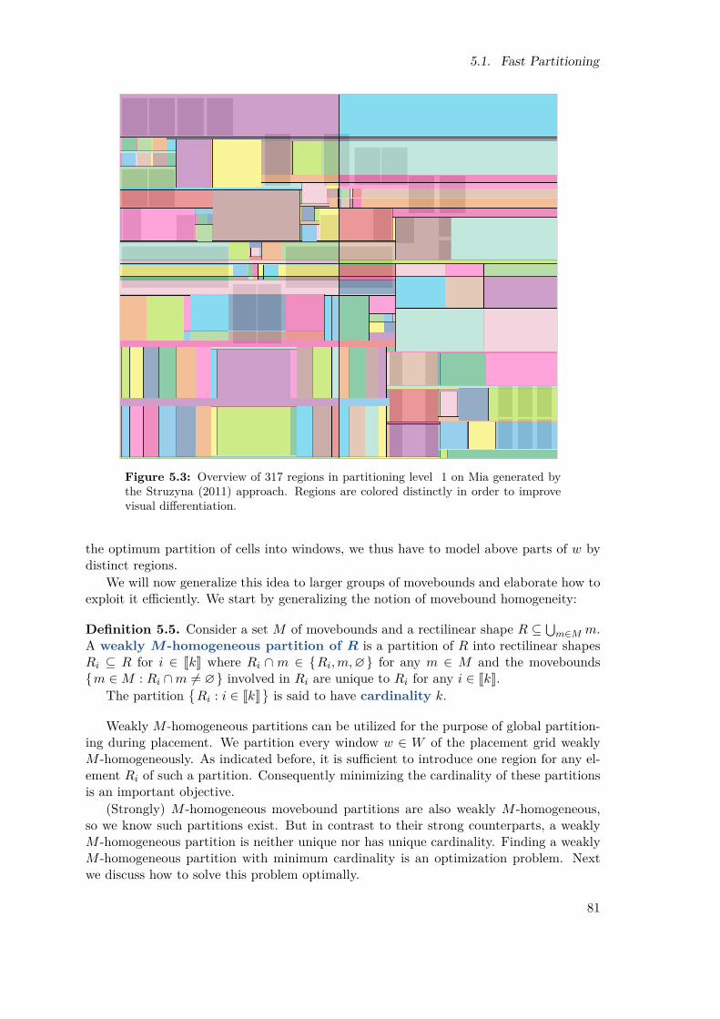
5.1. Fast Partitioning
Figure 5.3: Overview of 317 regions in partitioning level 1 on Mia generated bythe Struzyna (2011) approach. Regions are colored distinctly in order to improvevisual differentiation.
the optimum partition of cells into windows, we thus have to model above parts of w bydistinct regions.
We will now generalize this idea to larger groups of movebounds and elaborate how toexploit it efficiently. We start by generalizing the notion of movebound homogeneity:
Definition 5.5. Consider a set M of movebounds and a rectilinear shape R ⊆ ⋃m∈M m.A weakly M-homogeneous partition of R is a partition of R into rectilinear shapesRi ⊆ R for i ∈ JkK where Ri ∩ m ∈ Ri,m,∅ for any m ∈ M and the moveboundsm ∈M : Ri ∩m 6= ∅ involved in Ri are unique to Ri for any i ∈ JkK.
The partitionRi : i ∈ JkK
is said to have cardinality k.
Weakly M -homogeneous partitions can be utilized for the purpose of global partition-ing during placement. We partition every window w ∈ W of the placement grid weaklyM -homogeneously. As indicated before, it is sufficient to introduce one region for any el-ement Ri of such a partition. Consequently minimizing the cardinality of these partitionsis an important objective.
(Strongly) M -homogeneous movebound partitions are also weakly M -homogeneous,so we know such partitions exist. But in contrast to their strong counterparts, a weaklyM -homogeneous partition is neither unique nor has unique cardinality. Finding a weaklyM -homogeneous partition with minimum cardinality is an optimization problem. Nextwe discuss how to solve this problem optimally.
81

Chapter 5. Global Placement
Figure 5.4: Overview of 166 regions in partitioning level 1 on Mia generatedbased on M -homogeneous partitions of all windows using Lemma 5.4.
Definition 5.6. For a setM of movebounds the movebound graph GM is the directedgraph GM :=(M,EM ) where
EM :=
(m0,m1) : mi ∈M, m0 ∩m1 6= ∅, m1 6⊆ m0.
Definition 5.6 is motivated as follows: Consider a weaklyM -homogeneous partition Rifor i ∈ JnK of rectilinear shape R. Suppose m ∈ M satisfies m 6⊆ Ri for any i ∈ JnK butm ∩ R 6= ∅. If (m,m′) ∈ EM , m ∩m′ and m′ \m 6= ∅ must be covered by a different Riby weak movebound homogeneity. Consequently also m′ satisfies m′ 6⊆ Ri for any i ∈ JnK.
We now elaborate formally, how this reduces the identification of certain importantmovebounds to a reachability problem in GM . As a first step, we examine a particular setof moveboundsM ′ ⊆M which are sufficient for finding weaklyM -homogeneous partitions:
Proposition 5.7. Consider a set of moveboundsM and a rectilinear shape R ⊆ ⋃m∈M m.Let M ′ ⊆M be the movebounds reachable from
S :=m ∈M : m ∩R 6= ∅, m 6⊆ R
in GM . Further define M∗ :=M ′ ·∪m∗ for an artificial movebound m∗ with m∗ :=R \⋃m′∈M ′m
′.In this context any (strongly) M∗-homogeneous partition Ri of R is weakly M -
homogeneous.
82

5.1. Fast Partitioning
Proof. For m′ ∈ M ′ we have Ri ∩ m′ ∈ ∅, Ri ⊆∅, Ri,m′
for any Ri by strong
M ′-homogeneity of Ri.Otherwise m ∈M \M ′, for which we claim Ri ∩m ∈ ∅,m for any Ri: As m 6∈M ′,
for any m′ ∈M ′ we have (m′,m) 6∈ EM by choice of M ′. By Definition 5.6 of GM , for anym′ ∈ M ′ thus either m′ ∩m = ∅ or m ⊆ m′. By definition this is also the case for m∗.Consequently m is strongly M∗-homogeneous. If Ri ∩m = ∅ there is nothing to show.Otherwise m ⊆ Ri as both Ri and m are strongly M∗-homogeneous.
Note that by choice of m∗ in Proposition 5.7, R ⊆ ⋃m∈M∗m. Thus a strongly M∗-homogeneous partition of R exists.
Next we extend the motivation for Definition 5.6 of GM inductively. This establishesa lower bound on the cardinality of any weakly M -homogeneous partition:
Lemma 5.8. Consider a set of movebounds M , a rectilinear shape R ⊆ ⋃m∈M m and
S,M ′ ⊆ M as defined in Proposition 5.7. Further let Ri for i ∈ JnK be any weakly M -homogeneous partition of R. In this case Ri ∩m′ ∈ Ri,∅ for all m′ ∈M ′ and i ∈ JnK.
Proof. Let m′ ∈ M ′. We assume m′ ∩ R 6= ∅ as otherwise there is nothing to show. Bydefinition of M ′ there is a path P = (m0, . . . ,mk,m
′) in GM where m0 ∈ S. We useinduction on the length of a shortest such S-m′-path P .
For the induction basism0 = m′ and thusm′ ∈ S. By definition of S we havem′\R 6= ∅which implies m′ ∩Ri 6= m′ for any Ri ⊆ R. As Ri is a weakly M -homogeneous partition,Ri ∩m ∈ Ri,∅.
In the induction step Ri ∩mk ∈ Ri,∅ for any Ri. By choice of P as shortest S-m′-path, we have m′ 6∈ S. As m′ ∩R 6= ∅, this implies m′ ⊆ R. By the edge
(mk,m
′) ∈ EM ,we obtain ∅ 6= mk ∩m′ ⊆ m′ ⊆ R and m′ 6⊆ mk.
As Ri for i ∈ JnK are a partition of R, there is an Rj with Rj ∩ mk ∩ m′ 6= ∅. Byinduction hypothesis Rj ∩mk = Rj . As m′ 6⊆ mk, m′ \mk 6= ∅ by which m′ \Rj 6= ∅ i.e.Rj ∩m′ 6= m′. As Rj ∩m′ ∈ ∅,m′, Rj due to weak movebound homogeneity, we musthave Rj ∩m′ = Rj . As Ri for i ∈ JnK are a partition of R and particularly disjoint to Rj ,there is no Ri with Ri ∩m′ = m′. Thus Ri ∩m′ ∈ ∅, Ri .
We can use this lower bound of Lemma 5.8 to analyze the construction of Proposi-tion 5.7. As it turns out, this weakly M -homogeneous partition in fact has minimumcardinality:
Theorem 5.9. Consider a set of movebounds M and a rectilinear shape R ⊆ ⋃m∈M m.The weakly M -homogeneous partition constructed in Proposition 5.7 has minimum cardi-nality.
Proof. Let M∗ as defined in Proposition 5.7. By Lemma 5.8 any weakly M -homogeneouspartition of R is strongly M∗-homogeneous. By Definition 5.2 strongly M∗-homogeneouspartitions are unique and particularly have unique cardinality. Consequently the (unique)cardinality of a strongly M∗-homogeneous partition of R is a lower bound on the mini-mum cardinality of any weakly M -homogeneous partition of R. Since the partition ofProposition 5.7 attains this lower bound, it has minimum cardinality.
Using Theorem 5.9 we can compute weakly M -homogeneous partitions as fast asstrongly ones:
83

Chapter 5. Global Placement
Corollary 5.10. Consider a set of movebounds M and a rectilinear shape R ⊆ ⋃m∈M m.We can compute a weakly M -homogeneous partition of R with minimum cardinality
O(ρ log ρ+ |M |ω(log ρ+ logω))
where ρ denotes the size of representations for R and all movebounds m ∈M and ω is thesize of a representation of the strongly M -homogeneous partition of R.
As we discuss shortly, we did not implement the algorithm of Corollary 5.10. Insteadwe make use of a simpler approach which suffices in practice. Thus Corollary 5.10 is notcentral, which is why we only outline essential ideas of a technical proof here:
Proof (sketch). We can adapt the sweep-line algorithm of Proposition 5.3 to computea graph G = (M,E) with the following properties: G has O(ω) edges and for anym0,m1 ∈ M there is a m0-m1-path in G if and only if there is one in GM . Thus wecan compute M ′ ⊆ M reachable from S (cf. Proposition 5.7) in G instead of GM whichtakes O(ω) running time.
Finally by Theorem 5.9 it is sufficient to compute a stronglyM∗-homogeneous partition(cf. Proposition 5.7). As R ⊆ ⋃m∈M∗m, this partition exists. It can be computed in thestated running time by Proposition 5.3.
As mentioned, in practice we avoid making our sweep-line implementation even moreinvolved. Instead of M ′, we work with a superset N with M ′ ⊆ N which is easierto compute: We again start with the M -homogeneous partition Ri for i ∈ JnK of A.Afterwards we determine connected components in a modified, undirected moveboundgraph G′M :=
(M,E′M
)where
E′M :=m0,m1 : mi ∈M,m0 6= m1 and m0 ∩m1 6= ∅
.
By traversing all Ri and their involved movebounds, we can identify N as the nodesreachable from S in G′M . In particular, we thereby can avoid constructing G′M explicitly.Using the well-known union-find data structure (Tarjan 1975) this takes O(ω · α(|M |)),where α denotes the inverse Ackermann function.
Recall that by Definition 5.6 the movebound graph GM is directed and only introducesedges under additional requirements. Consequently M ′ ⊆ N as claimed.
With the usual artificial movebound, we can actually determine a strongly N∗-homogeneous partition from Ri. This can be done by sorting all rectangles in repre-sentations of all Ri and has already been elaborated in the second part of the proof ofLemma 5.4. Since M ′ ⊆ N , the result of this operation is strongly M∗-homogeneous andthus in fact weakly M -homogeneous by Proposition 5.7.
Since M ′ ⊆ N , the result of our implementation is not necessarily a partition ofminimum cardinality. But this de facto is not a huge restriction, since the circumstancesof extra movebounds in N \M ′ happens rarely in practice, in particular not at all in theexperiments presented in Section 6.2.5.1.3 Weakly Movebound Homogeneous RegionsWe can use Corollary 5.10 in each window w ∈ W to find a set of regions R(w) that isminimum for modelling partitioning accurately globally. This can be achieved using theapproach of Lemma 5.4 while substituting the strongly M -homogeneous partition by aweakly one.
84

5.1. Fast Partitioning
Figure 5.5: Overview of 70 regions in partitioning level 1 on Mia generated basedon weakly M -homogeneous partitions of the windows.
This improves the number of created regions drastically. To illustrate this, we recon-sider the instance Mia for which different region creation algorithms have been depicted inFigures 5.3 and 5.4. The 70 regions generated based on weaklyM -homogeneous partitionsof the windows are shown in Figure 5.5. As initially intended, we can clearly identify largegroups of former regions that could be elided by making use of weak M -homogeneity.
Although the output of this approach is optimum in the sense of Theorem 5.9, itcan not be computed quickly. Computing regions so far requires querying moveboundsand blockages for each w ∈ W . Due to the recursive nature of partitioning based globalplacement, we can have millions of windows – especially in the last levels and especiallyon chips with large chip area.
But we can avoid using any quad-trees for this purpose whatsoever. Instead we exploitthe grid structure of the windows W , which we have not done at all so far.
Proposition 5.11. Consider a set of movebounds M in chip area A and a set of gridwindows W subdividing A. We can partition all w ∈ W into weakly M -homogeneousregions R(w) with minimum cardinality in
O(µ logµ+ |M |γ(logµ+ log γ) +
(γ + |M |) log|W |+ ω
)running time, where ω is the size of representations of the output R(w) for all w ∈W , µ isthe size of representations for all movebounds m ∈M and γ is the size of a representationfor the (strongly) M -homogeneous partition of A.
85
Chapter 5. Global Placement
Proof. Let S :=m ∈M :6 ∃w ∈W with m ⊆ w and M ′ ⊆M the movebounds reachablefrom S in GM . S and M ′ are the union of all Sw and M ′w used for finding weakly M -homogeneous partitions of w in Theorem 5.9. Further we specify the artificial moveboundm∗ by m∗ :=A \⋃m∈M ′m and denote M∗ :=M ·∪m∗ .
Let Hi for i ∈ JnK be a strongly M∗-homogeneous partition of A. By Theo-rem 5.9, for each w ∈ W the partition Hw :=
Hi ∩ w : Hi ∩ w 6= ∅, i ∈ JnK
is weakly
M -homogeneous and has minimum cardinality. We will define regions R(w) according tothe partition Hw of w ∈W .
We do so by using the grid structure of W as follows: For any point p ∈ A, we can finda window w ∈W containing p by binary search in O(log|W |) running time. If p is exactlyon the border between neighboring windows, there can be up to four such windows.
We can determine whether m ∈ S by checking m ⊆ w for a single w ∈ W : If such aw exists, it is a window closest to the center of m. Thus we detect m ∈ S by checking allthose constantly many closest windows. This takes O(µ+ |M | log|W |) running time forall movebounds together.
Next we use Corollary 5.10 to compute the graph G with O(γ) edges containing a m0-m1-path if and only if the movebound graph GM does so. Thus we determine M ′ as themovebounds reachable from S in G in O(γ) running time. By Corollary 5.10 computingG and all Hi can be done in O(µ logµ+ |M |γ(logµ+ log γ)
)running time.
Afterwards for each rectangle h ∈ Hi and each i ∈ JnK, we traverse all windows wintersecting h. Again we can find those windows by binary search exploiting the gridstructure of W in O(log|W |) running time. For each such pair (h,w) we either introducea new region in R(w) or add h ∩ w to r of an existing region r ∈ R(w) for Hi. Thisconsumes O(γ log|W |+ ω
)running time overall.
In order to complete the construction of regions, we also need to consider blockages,which Proposition 5.11 does not do so far. We have two options to incorporate blockages:
It would be possible to subtract blockages B from the overall chip image A beforeapplying Proposition 5.11. This is an elegant solution, but increases both γ and ω in therunning time. In particular this can increase the complexity of the decomposition of winto r for r ∈ R(w), even for w ∈W not intersecting B.
In order to avoid this effect, we first apply Proposition 5.11 and afterwards subtractblockages from regions. On the one hand, this introduces the overhead of finding theseregions that intersect B. On the other hand, we thereby avoid any side effects on regionsdisjoint from B. This approach has the following running time:
Lemma 5.12. Consider a rectilinear shape B of blockages represented by rectangles bi fori ∈ JnK. Let R(w) be regions for all windows w ∈W of a grid. We can compute r \B forall r ∈ R(w) and w ∈W in
∑i ∈ JnK
log|W |+∑
r ∈ R(w) : w ∩ bi 6= ∅ρr
running time, where ρr denotes the size of a representation of r.
Proof. We process each bi one after another. For each i ∈ JnK we compute the setWi :=w ∈W : w ∩ bi 6= ∅ in O(log|W |) running time using binary search on W . Thisargument has already been discussed in the proof of Proposition 5.11. Subsequently weiterate all r ∈ R(w) for w ∈Wi and subtract bi from r in O(ρr) running time.
86

5.1. Fast Partitioning
Both Proposition 5.11 and Lemma 5.12 reflect the running time of our actual imple-mentation. We now discuss two purely theoretical improvements that are not used inpractice:
First of all, we can avoid binary search entirely: All windows, regions and blockageshave integer coordinates. For each dimension separately, finding the grid line next to agiven coordinate x ∈ Z thus can be accomplished inO(1) using a lookup table. This lookuptable though is very large, namely linear in width and height of A (which is exponentialin the input). Practical experiments showed that the overhead of populating the lookuptable outweighs the speedup for querying windows. Thus we use binary search both intheory and practice.
Secondly Lemma 5.12 always traverses all regions of the windows Wi while actuallyonly those intersecting bi would be sufficient. Querying those regions efficiently is not aneasy task. Falling back to one quad-tree for each window w ∈ W storing region areas forr ∈ R(w) is not an option: r is a rectilinear shape which can not be stored in generaland storing BB(r) instead still leads to regions considered unnecessarily. Moreover theoverhead of managing separate quad-trees for each w ∈ W would be drastic – especiallyin the last levels of global placement.
Finally the overhead is expected to be minor overall: In the first levels, there are fewregions altogether and even considering all of them for each bi would be manageable. Incontrast to this we have millions of regions in the final levels of global placement. But hereeach window consists of very few regions, usually even only a single one. Thus the numberof unnecessarily considered regions remains small. This is why we use the approach inpractice exactly as described in Lemma 5.12.
Now we want to compare the region construction in Lemma 5.4 against Proposition 5.11plus Lemma 5.12: Clearly the latter combination finds strictly superior regions for par-titioning. It computes regions R(w) with weakly M -homogeneous areas with minimumcardinality. Even though we do not guarantee minimum cardinality in practice, we stilldemonstrated to significantly reduce the number of regions.
Besides output quality, also the required running time is preferable: For a start, therunning time can be stated precisely as it does not use quad-trees any longer. Furthermoreboth Proposition 5.11 and Lemma 5.12 avoid all operations done for each and every w ∈Wand r ∈ R(w) respectively. As a consequence this combination is very valuable in practice– especially in the last levels of global placement. A detailed comparison of different regionconstruction paradigms is presented in Section 6.2.
Finally we’d like to close this section by a few practical remarks:BonnPlace supports non-uniform target densities. This is modeled by certain
density-rectangles d ⊆ A specifying a deviating target density inside d. We incor-porate these similarly as blockages are handled in Lemma 5.12. The only difference isthat we alter the capacity of r ∈ R(w) instead of reducing r.
Furthermore computing regions for partitioning not only requires to calculate capacitiesonly. In addition we also need to find the center of gravity of r for each region r. Thiscan easily be computed during a final step as the weighted average of centers of a ∈ rweighted by a’s area. But this is computationally difficult as it averages products of 32-bitand 64-bit integers (the areas). Those products can not be represented by 64-bit integerswhich is the maximum available to us. In order to overcome this, we compute thoseproducts as floating point numbers and make use of the compensated summation methodof Kahan (1965). This makes the error of summing n floating point numbers independentof n (Higham 1993).
87

Chapter 5. Global Placement
Algorithm 5.1: Self-Stabilizing BonnPlaceInput : Cells C.Output: Locations pos(c) for all cells c ∈ C.
1 pos :≡ 0, iter := 02 while not BreakCondition(pos, iter) do3 foreach c ∈ C do4 Connect c to a new pin at position pos(c) via a virtual net of weight
0.01 · iter.5 Partitioning-based BonnPlaceGlobal6 BonnPlaceLegalization7 Delete virtual nets8 if timing_optimization_enabled then9 BonnLayerAssignment
10 BonnRefinePlace11 BonnPlaceLegalization12 if routability_driven_placement_enabled then13 CongestionAvoidance14 Store current placement as pos, iter := iter + 1
5.2 Self-Stabilizing BonnPlaceWe now present the self-stabilizing BonnPlace framework (Brenner et al. 2015) forGlobal Placement. This framework is a versatile algorithm based on various com-ponents of the BonnTools suite (Korte, Rautenbach and Vygen 2007) developed at theResearch Institute for Discrete Mathematics of the University of Bonn. It can optimizenetlength as well as timing properties (Section 5.3) and routability (Section 5.4).
Self-stabilizing BonnPlace combines the two strongly opposing placement strategiesdescribed in Section 2.4: force-directed and partitioning-based placement. In essence weperform multiple iterations of global placement followed by (standard cell) legalization.In our case this is BonnPlaceGlobal plus BonnPlaceLegalization.
Each iteration learns from previous ones. The insights gained in past iterations aretransferred purely via virtual nets which we call forces. We thereby artificially pullcells towards some position derived from former iterations. Algorithm 5.1 outlines thisplacement strategy.
This approach provides the flexibility to incorporate multiple optimizations for var-ious placement objectives and constraints. We demonstrate how our placement schemestabilizes towards a solution meeting opposing placement goals. This justifies the nameSelf-Stabilizing BonnPlace.
5.2.1 General FrameworkA key ingredient of our tool is the partitioning-based global placement algorithm Bonn-PlaceGlobal (Algorithm 5.1, line 5). As described in Section 5.1, BonnPlaceGlobaliterates analytical placement and flow-based partitioning in multiple levels.
The analytical placement, which is computed in the very first level 0 of each iteration,is of particular interest. In this level the placement grid is trivial i.e. contains only a
88

5.2. Self-Stabilizing BonnPlace
single window. Referring to the notion of SimPL (Kim, Lee and Markov 2012, 2013),the remainder of BonnPlaceGlobal plus BonnPlaceLegalization can be seen aslegalization of this initial placement.
Over the course of iterations, level 0 placements contain fewer overlaps (cf. Figures 5.6and 5.7 and Section 6.3). The extended spreading predicts inevitable distortions for achiev-ing legality. It also helps BonnPlaceGlobal anticipating the effects of partitioningdecisions more accurately. On the other hand, those level 0 placements still optimize net-length on a global scale. Consequently in later iterations we can legalize these locationswith fewer movement and smaller netlength increase.
BonnPlaceGlobal (Brenner, Struzyna and Vygen 2008; Struzyna 2011) optimizes(weighted) quadratic netlength using the clique-netmodel for nets with few pins and thestar-netmodel otherwise (Brenner and Vygen 2001). For pure netlength minimization weinstead make use of a combination of the bound-to-bound net model (B2B) with a super-linear distance scaling factor (Struzyna 2013). As of iteration one, we use the currentplacement to determine the outer pins of nets for the B2B net model. Thus we can avoidthe computation of multiple QPs with B2B in order to stabilize the solution.
The result of BonnPlaceGlobal respects the target density accurately, but con-tains overlaps that need to be resolved locally. For this purpose we use Bonn-PlaceLegalization of Brenner (2012) (Algorithm 5.1, line 6). This algorithm mini-mizes quadratic movement by incrementally clearing overlaps similar to the SuccessiveShortest Path Algorithm (Edmonds and Karp 1972; Tomizawa 1971).
(a) Iteration 0 (b) Iteration 1 (c) Iteration 2 (d) Iteration 3
Figure 5.6: Spreading of cells on Renaud in the first analytical placement in thefirst four iterations. Each cell location is drawn as single blue point.
In the first iteration (iter 0) of our self-stabilizing global placer, we do not knowany legal placement. Thus we skip introducing any forces whatsoever. Afterwards theforces (cf. Section 5.2.2) are respected throughout BonnPlaceGlobal i.e. they affectthe solution in each level and not only the global analytical placement in level 0.
In contrast to other force-directed approaches, we spend more running time for a singleiteration. On the other hand, each iteration not only results in a placement respecting allconstraints (legality, movebounds, target density, blockages cf. Section 2.2) but also is ofhigh quality (Struzyna 2011, 2013).
This allows us to reduce the number of iterations drastically: SimPL (Kim, Lee andMarkov 2012, 2013) requires∼50 iterations, ePlace (Lu, Chen et al. 2015) even more than250. In contrast, for self-stabilizing BonnPlace depending on additional optimizationobjectives (Sections 5.3 and 5.4) 5 to 15 iterations suffice. We optimize elaborately andthus reliably in each iteration, which allows a steeper increase of forces.
89

Chapter 5. Global Placement
5.2.2 ForcesIn our placement algorithm, forces are used to transfer information and to stabilize theplacement procedure. The higher the quality is of information that we get from earlieriterations, the greater is the efficiency of forces. We spend much effort on legalizing eachanalytical placement to a solution of high quality. Transferring this kind of collectedinformation by means of forces is effective.
(a) Iteration 0 (b) Iteration 1 (c) Iteration 2 (d) Iteration 3
Figure 5.7: Spreading of cells on Franziska in the first analytical placement in thefirst four iterations. Each cell location is drawn as single blue point.
We add forces at the beginning of an iteration (Algorithm 5.1, lines 3 to 4). Forthis construction of forces we can use placement information pos stored at the end of theprevious iteration (Algorithm 5.1, line 14). The first iter 0 is performed without forces.During each subsequent iteration iter > 0 of self-stabilizing BonnPlace, there is exactlyone force pulling at each cell.
Forces are modeled as artificial two-terminal nets connecting any cell to some fixedposition on the chip. Those nets are handled exactly the same way as regular nets. Inparticular artificial nets affect the distribution of cells during the analytical placements,but have no (direct) influence on other steps minimizing movement, e.g. flow-based parti-tioning.
For each cell c in the set of circuits C, the artificial force-net is connected to the centerof c. The fixed pin of the force-net is located at pos(c), i.e. the location of c determined inthe previous iteration. This position is called the target point of the force pulling at c.We have experimented with different target points incorporating further past iterations,but this could not improve practical results (Hoppmann 2014).
The weight of force nets increases in each iteration to stabilize the placement. Higherstability is expressed by decreasing cell movement between two consecutive iterationsand converging analytical and legalized placement netlengths. On the one hand, forceshave to be very effective. As we legalize analytical placements with high effort, we wantto transfer as much of the information gained in previous iterations as possible. Inparticular we should induce a significant cell spreading in the analytical placement ofsubsequent iterations. On the other hand, force weights need to be chosen such thatartificial nets are not predominant for netlength minimization. We need to provideguidance, while guaranteeing enough flexibility for our partitioning-based global placerBonnPlaceGlobal.
90

5.3. Routability-Driven Placement
We achieve this by a weight of 0.01 · iter. The average non-artificial net weight is1. Thus our choice of force-weights defines a 1 %-increase in each iteration compared tothe standard net weight. Different uniform and non-uniform force weights provided nobenefits in practice for minimizing netlength (Hoppmann 2014) which is why we stick tothis simple scheme. Increasing force-weights non-uniformly is of particular interest foroptimizing timing characteristics and will be discussed in Section 5.4 in detail.
The impact of forces to the quadratic placement is shown in Figures 5.6 and 5.7 ontwo industrial designs. We see the analytical placement computed in level 0 of Bonn-PlaceGlobal, where we only have one window representing the whole chip area. Weshow the these solutions over the course of the first four iterations (iter ∈ J4K). The spread-ing is already significant, but far from giving a legal solution. This demonstrates how weare able to balance increased spreading and freedom for BonnPlaceGlobal. Althoughwe are able to provide significant guidance and enforce stability, we still leave considerablymany choices for this partitioning-based placer.
When a legal placement is found, we delete forces (Algorithm 5.1, line 7). In thefollowing iteration, new forces will be computed.
5.2.3 Breaking ConditionsThe general breaking condition for the overall loop is a user-specified maximum number ofiterations – typically around 5 to 10. But the Self-Stabilizing BonnPlace frameworkis very flexible and allows further extensions.
In order to save running time, we can skip remaining iterations based on the cells’movement in the last iterations. As future iterations with higher force weights are expectedto deviate less from previous placements, we anticipate to miss little improvement.
As we will demonstrated in Section 6.3, optimization objectives vary non-monotonicallyover the course of iterations. Thus we require the full number of iterations when aimingfor the best quality possible.
On the other hand, this is not always the actual objective in chip design. Dependingon the stage of the design process, sometimes placement algorithms are used to decidewhether a given netlist can be placed routably or with specified slack. We can easilyincorporate criteria to end our algorithm prematurely whenever a placement of sufficientquality is known.
5.3 Routability-Driven PlacementBesides minimizing netlength, our placer is able to improve the routability of a chip. Themain idea is to dynamically reduce placement density wherever routing becomes difficult.We achieve lowered placement density by artificially increasing the size of cells in suchsectors of the chip.
Our CongestionAvoidance routine (Algorithm 5.2) is called at the end of eachiteration (Algorithm 5.1, line 13) of Self-Stabilizing BonnPlace. The result of thisalgorithm, namely new sizes for all cells, serves as input for the following iteration.Updated sizes of cells affect global density, i.e. inflated cells consume more capacity duringflow-based partitioning. On the other hand, those size updates never change the actualphysical outline of a cell.
CongestionAvoidance consist of two major components: congestion estimation(line 1) and density adjustment (lines 2 to 12). In the following we discuss both thosesteps.
91

Chapter 5. Global Placement
Algorithm 5.2: CongestionAvoidanceInput : Grid G, cells C, locations pos(c) for c ∈ C, target/critical wire density
tgt/crit.Output: Adjusted size(c) for all c ∈ C.
1 Use BonnRouteGlobal as congestion estimation on G2 while congested_edge_percentage < 10% and crit > tgt do3 crit := maxtgt, crit− 5 %4 foreach tile window w ∈ G do5 Compute criticality(w) w.r.t. crit6 Choose a ∈ [0, 1]7 foreach tile window w ∈ G do8 foreach cell c ∈ w do9 if criticality(w) > 0 then
10 size(c) := size(c) + a · inflate(c, w)11 else if criticality(w) ≤ 0 then12 size(c) := size(c) + shrink(c, w)
13 return size
5.3.1 Congestion EstimationWe use an actual global router for estimating congestion (Algorithm 5.2, line 1). Suchan algorithm roughly decides how nets are routed, but avoids finding a routing that isactually legal w.r.t. various distance constraints. In particular it determines a predictionof the number of wires crossing certain areas of the chip. We measure congestion basedon this global routing.
Note that during Self-Stabilizing BonnPlace (cf. Algorithm 5.1) Congestion-Avoidance is always applied to a legal placement. A global routing engine works beston legal placements, as predicting congestion accurately is much harder otherwise. Thusalso CongestionAvoidance benefits from the effort spent on legalizing the placementthoroughly.
The global router we rely on is BonnRouteGlobal (Müller, Radke and Vygen2011). This tool considers a coarse three-dimensional grid that partitions the routingarea on all layers. In this grid the global routing problem can be modeled as Min-MaxResource Sharing Problem where resource allocation (routing capacity along grid-edges) is balanced among customers (nets). Assuming individual nets can be routed near-optimally, this approach is proven to find near optimum solutions for the overall globalrouting problem very efficiently.
Moreover this algorithm is also very relevant in practice. In particular it is used inmultiple stages of the IBM chip design process, most notably as first step of detailedrouting (Ahrens et al. 2015; Gester et al. 2013).
For our congestion analysis we align the global routing grid to the placement grid. Asa consequence BonnRouteGlobal estimates exactly the routing requirements causedby our partition of cells into windows. In order to limit running time, we avoid usingthe grid of the final placement level. Instead we use a coarser grid, more precisely of the
92

5.3. Routability-Driven Placement
maximum level during which windows exceed a user-specified number of routing tracks.Naturally we need a fast congestion estimation that can be computed frequently. For
our purposes we also prefer a rough, pessimistic estimation over a more accurate andpossibly optimistic one. This is due to the fact that we want to optimize our placementto be routable easily, rather than barely and with huge effort. Considering a pessimisticrouting estimation more clearly shows where we need to improve the placement.
Thus we adjust standard BonnRouteGlobal in two ways for our purposes: On theone hand, we reduce the number of phases of the Resource Sharing Algorithm to asingle one. On the other hand, we route each net with artificially restricted search space.Instead of leaving the freedom to route it arbitrarily (possibly with large detour to avoidcongestion hotspots), we narrow the search space to the net’s bounding box (plus fewgrid windows). Due to this, routing hotspots can be observed more clearly. Due to bothchoices, we lose theoretical guarantees but make this approach viable in practice.
5.3.2 Density AdjustmentsWith a congestion estimation at hand, Algorithm 5.2 adapts the density of the placement.This is done in two steps similar to Brenner and Rohe (2003): assigning each windowof the grid a routing criticality (lines 2 to 5) and distributing inflations based on thiscriticality (lines 7 to 12). We now elaborate those steps.
In contrast to Brenner and Rohe (2003), CongestionAvoidance manages a dynami-cally adapting congestion target crit. We lower crit maximally towards tgt s.t. at least 10 %of the routing edges have a congestion of at least crit. Here tgt denotes a user-specifiedcongestion target which is usually chosen around 80 % to 90 %.
Based on this congestion target crit and the actual estimated routing congestion, wedetermine routing edge criticalities. These edge criticalities in the interval [0, 1] are derivedby mapping congestion below crit to 0, above l to 1 and interpolating linearly in [crit, l ].Here l denotes a user-specified congestion cutoff (usually 130 %).
Afterwards we designate criticality(w) ∈ [0, 1] to the grid windows (lines 4 to 5).These criticalities are chosen as the average of pin density in w and the edge criticalitiesof incident routing edges of w.
But inflations can not only be increased, but also reduced. In order to downsize cellsin a window, all adjacent edges are required to have criticality 0. If this is the case, wesimilarly interpolate a routing edge uncriticality in [−1, 0] where congestion crit is mappedto 0 and congestion 0 % to −1. Based on this, criticality(w) ∈ [−1, 0] is averaged as before.Reducing cell inflation is essential to recover space in uncongested sectors of the chip.
The distribution of inflations is performed in analogy to Brenner and Rohe (2003)(lines 7 to 12). At this point we have computed criticality(w) ∈ [−1, 1] for each windoww. We then compute the area increment of w as
criticality(w) · ι ·∑c∈w
size(c)
where ι is a user-specified inflation emphasis (usually 80 %). This area increment of w isthen distributed to c ∈ w proportionally to the number of pins of c. We thereby ensurethat no cell is shrinked below its original size.
In order to ensure that the inflated cells can still be placed on the chip at all, weinitially choose a maximum scalar a ∈ [0, 1] for which this is possible. This scalar appliesto all inflations and shrinkages of any cells.
93

Chapter 5. Global Placement
Adapting the criticality threshold crit is essential. On the one hand, it results incautiously computed inflations that targeted congestion hotspots precisely. On the otherhand, we crucially aim at reducing congestion globally towards tgt, even below 100 %.Barely routable chips make detours inevitable, which has a negative effect on other designobjectives. Thus it is necessary to optimize for maximum congestion tgt to make routingeasier. Dynamically adapting our critical congestion crit is an important component forthis. It is very effective in practice as we demonstrate in Section 6.4.2.
5.4 Timing-Aware PlacementThe versatility of Self-Stabilizing BonnPlace is especially useful for optimizing timingcharacteristics (Algorithm 5.1, lines 8 to 11). Besides good routability, this is the mostimportant objective during placement for modern technology nodes. Moreover optimizingthis objective is required to evaluate timing-driven macro placements as obtained byBonnMacro (cf. Chapter 4).
Our framework applies two different methods to resolve timing problems: we optimizethe assignment of nets to routing layers as well as locally move circuits purely based ontiming properties.
Remember that we assume Self-Stabilizing BonnPlace is applied in a linearizedtiming model (cf. Section 2.2.2). Due to this timing optimization runs more efficiently.
As first stage of our internal timing optimization, we run BonnLayerAssignment(Algorithm 5.1, line 9). This module of the BonnTools suite specifically targets criticalnets. It improves the delay of such nets by assigning those to higher layers and recom-mending wider wires. Both those changes lead to lowered resistance and thus improvedtiming.
Naturally especially critical nets compete for limited routing resources on the fastestlayers. BonnLayerAssignment heuristically respects these routing capacities withouthaving to compute an actual global routing. On the other hand, we can also operatethis tool in an optimistic mode where such constraints are not applied. It makes senseto use this mode to obtain worst slack bounds e.g. for evaluating timing-driven macroplacements.
As described in Section 2.2.2, the delay of long nets differs greatly between layers.Thus it is important to first assign long connections across the chip to the fastest layers.Only under this condition we can apply our local placement optimization based on timing.
For this purpose (Algorithm 5.1, line 10) we use another component of the BonnToolssuite: BonnRefinePlace (Bock et al. 2015; Bock 2010). This tool relocates a predefinedratio of cells in the most critical nets to decrease the overall timing criticality. In this step,cells are moved such that critical paths are shortened and detours are avoided. Thisis achieved by a local search for timing optimal positions of single circuits. In orderto overcome local minima, small clusters of neighboring critical cells can also be movedsimultaneously. Typically this approach allows to shorten critical paths significantly incase it is sufficient to move only some of the cells.
The resulting positions of BonnRefinePlace are not necessarily legal. Using theaforementioned BonnPlaceLegalization (Brenner 2012) once again we can resolve alloverlaps in the placement (Algorithm 5.1, line 11). As only a small fraction of cells wasmoved, legalization is efficient and causes little movement as well as degradation in timing.
These refined positions serve as force target points in the next iteration. Moreoverwe emphasize the importance of cells moved by BonnRefinePlace. To do so, weadditionally increase the force weight by 50 % for those circuits. The raised force weights
94

5.4. Timing-Aware Placement
persist in subsequent iterations until the standard force weight has caught up or the cellis moved once again.
With this weighting scheme, we achieve two contrary characteristics: On the onehand, our placer is strongly encouraged to retain similar positions for critical cells in thefuture. On the other hand, in subsequent iterations different cells might become the mosttiming critical. Thus our weight emphasis decays for cells having been formerly critical.We thereby can improve the timing characteristics of placement solutions in subsequentiterations.
Previous versions of Self-Stabilizing BonnPlace additionally updated net weightsbased on timing criticality (Brenner et al. 2015). This turned out to be harmful for moderntechnology nodes and thus is not done any longer.
All described steps for timing optimization change the placement or the layer assign-ment. Either way, these changes directly affect global routability. This is why it is moreeffective to estimate congestion at the end of an iteration in our placement scheme.
To optimize timing thoroughly, we usually perform 15 iterations of timing-driven Self-Stabilizing BonnPlace. Thereby we delay inclusion of BonnLayerAssignment toiteration 1 and BonnRefinePlace to 2. Gradually adding optimization steps helpsin conjunction with CongestionAvoidance as particularly BonnLayerAssignmentsignificantly changes global routability. Thus our placer benefits from the opportunity toadapt the placement accordingly.
For estimating macro placements, less iterations are sufficient. Usually we restrictourselves to 5 iterations whereby we skip optimizing routability and run BonnLayerAs-signment in the mode that disregards routability.
As a closing remark we want to point out the versatility of Self-Stabilizing Bonn-Place. Incorporating further timing optimization techniques which deviate from previ-ous placements even more significantly, e.g. logic optimization or latch clustering, seempromising for future evolutions of our framework.
95


Chapter 6
Experimental Results
This chapter is devoted to the performance of various placement algorithms that havepreviously been discussed. We examine our tools by experiments both on recent real-world instances from industry and on benchmark chips.
Section 6.1 provides an overview of all designs and the benchmarking environment.In Section 6.2 we revisit the running time effects of our improved region construction asdiscussed in Section 5.1. Afterwards we concentrate on Self-Stabilizing BonnPlace(cf. Sections 5.2 to 5.4): We start with an analysis of the basic mode in Section 6.3,before we discuss the congestion-aware mode in Section 6.4 and the joint timing-drivenand congestion-aware variant in Section 6.5. Finally Section 6.6 analyzes our timing-drivenextension of BonnMacro which has been proposed in Chapter 4.
6.1 Test EnvironmentAn overview of all test instances considered in this chapter is presented in Table 6.1. Allinstances are real-world designs provided by our industrial partner IBM.
We test primarily on designs of the current technology nodes, but also include chal-lenging older test cases. Moreover we consider designs with millions of cells, many macrosand blockages as well as complicated movebounds.
Note that we consider multiple variants of one particular instance: Alex. Alex (v1) hasextra movebounds arising from the design hierarchy and Alex (v2) contains many extrablockages.
For technical reasons not all instances provide both timing and routing environments,which is why it is impossible to analyze all approaches on the entire testbed. In thefollowing chapters we consider subsets of the presented chips, for which the respectiveapproaches seemed most promising.
Unless stated otherwise, all experiments have been conducted on an Intel Xeon E5-2699 v4 CPU which runs at 2.2 GHz base frequency. The Intel® Turbo Boost Technologyis enabled with a maximum clock speed of 3.6 GHz. This processor has 22 physical coresproviding 44 threads via hyper-threading. Our machine is equipped with 378 GB of mainmemory.
Our code was compiled using clang version 7.0.0 on CentOS release 7.6 using optimiza-tion level 03. All mixed-integer and linear programs are solved using IBM ILOG CPLEXOptimization Studio 12.6 (CPLEX).
97

Chapter 6. Experimental Results
Chip T C L P N M B MD DB R CA[nm] [103] [103] [103] [%] [103] [mm2]
Anna 14 2 800 203 76 5 24 83 10 15 2.5× 2.5Rosemarie 14 7 941 359 140 9 58 9 13 6.5× 4.6Ida 22 19 67 19 2 1 7 0.2× 0.2Leo 22 31 9 94 34 4 66 1 12 0.8× 0.9Beate 22 41 141 43 10 1 7 0.3× 0.3Sonja 14 53 5 170 55 10 3 11 0.3× 0.4Anja 14 66 244 86 37 56 3 15 2.0× 4.1August 14 73 18 176 67 6 26 3 7 0.7× 0.4Rolf 7 75 222 72 1 8 0.2× 0.3Jannik 14 126 21 360 126 4 4 54 43 13 0.7× 1.7Conni 14 134 99 494 164 66 275 11 1.1× 1.3Falk 14 169 488 167 1 13 0.3× 0.3Lisa 14 171 294 271 121 4 70 2 15 1.5× 2.4Benedikt 22 264 37 837 267 2 29 3 13 0.5× 2.1Renaud 45 352 33 1 132 352 4 33 1 7 1.0× 1.1Viktor 22 382 142 1 551 444 6 5 2.4× 3.9Franziska 22 386 20 1 336 412 2 21 686 13 1.3× 1.7Meinolf 22 393 1 1 494 437 2 1 2 7 1.0× 0.8Iris 22 430 11 1 577 474 2 9 1 224 7 1.0× 0.9Gautier 45 1 362 2 926 5 136 1 478 4 29 14 101 8 4.0× 6.0Regina 14 1 385 37 4 266 1 495 1 2 22 3 384 15 1.9× 1.4Mia 14 1 499 35 4 625 1 625 84 20 3 710 15 1.8× 1.5Valentin 14 1 585 265 4 912 1 693 57 41 4 077 15 2.2× 1.7Rafael 32 1 946 7 008 5 983 1 920 1 982 51 8 487 11 3.2× 2.7Elias 14 5 132 372 16 262 5 408 24 23 19 395 15 2.5× 2.5Alex 14 8 484 3 262 24 906 8 955 380 35 16 222 15 6.1× 4.6Alex (v1) 14 8 484 3 262 24 906 8 955 361 380 35 16 222 15 6.1× 4.6Alex (v2) 14 8 484 3 262 24 906 8 955 301K 56 16 222 15 6.1× 4.6
Table 6.1: Overview of our testbed: For each chip the technology T in [nm], thenumber of cells C, non-standard cells L, pins P, nets N, movebounds M, blockagesB, distance bounds DB and routing layers R. Moreover the fraction MD of the chiparea covered by macros in [%] as well as the chip area CA in [mm2].
98

6.2. Partitioning with Movebounds
6.2 Partitioning with MoveboundsWe first examine the impact of different region construction strategies for Bonn-PlaceGlobal as discussed in Section 5.1. We compare different approaches duringGlobal Placement where all macros have fixed positions. In this context we do notconsider self-stabilizing yet, i.e. perform only a single iteration.
We compare three different approaches: The baseline has been presented in Lemma 5.4.In contrast to the original implementation of Struzyna (2011) it has been improvedto compute the (strongly) movebound homogeneous partition in polynomial time usingProposition 5.3.
An improved version of this strategy is referenced as M -homogeneous. It computesthe movebound homogeneous partition similarly, but in contrast only introduces a singleregion for each element of this partition. Moreover it manages blockages more efficientlyby exploiting the grid structure of windows using Lemma 5.12.
The final approach relies on a weakly M -homogeneous partition of windows. This hasbeen proposed in Proposition 5.11 and includes the same blockage handling mechanismas for the M -homogeneous case.
In a first analysis we reconsider the instance Mia which has already been visualizedmultiple times before (cf. Figures 5.1 to 5.5, pages 79 and 85). This instance is of particularinterest as it has the most challenging movebound structure. Figure 5.2 highlights theintricately overlapping movebound configurations.
The mentioned approaches on this particular instance are compared in Figure 6.1. Weanalyze different properties of all three mentioned approaches in the respective levels ofBonnPlaceGlobal. Since level 0 consists of a single, very efficient QP computationonly (without partitioning), the shown analysis starts with level 1.
On the left we see the number of introduced regions. The exponential increase inregions is intrinsic to recursive partitioning and particularly underlined due to the loga-rithmic scaling. The right of Figure 6.1 visualizes the total wall clock time spent in therespective levels for each strategy.
During the first levels of placement we see a drastic reduction in number of regions.The running time improvement obtained by considering fewer regions is even more obvious.The running time spent in level 2 in the baseline was 2:14 h, which could be reduced to29 min and 15 min with the strongly and weakly movebound homogeneous approaches.The substantial running time improvements are very much expected, since the number ofregions super-linearly contributes to the running time complexity of solving min-cost flowproblems in partitioning.
In the last levels of BonnPlaceGlobal the difference is marginal for two main rea-sons: For once windows become very small and thus intersect few movebounds. Conse-quently the constructed regions of all approaches are more and more similar until theycoincide for all approaches in the final level. On the other hand, our placer processesmultiple windows in parallel. This parallelization works best if there are sufficiently manywindows and compensates for marginal improvements on single, small instances.
A comparison on a larger testbed with more chips is presented in Table 6.2. Allinstances are ordered by increasing number of cells. For each chip we compare thesame region construction variants baseline (base), M -homogeneous (hom) and weaklyM -homogeneous (whom) as in Figure 6.1 in separate rows.
In the columns of Table 6.2 we show the total wall clock time of BonnPlaceGlobal(BPG WT), the wall clock time contribution of computing regions (BPG RC) as well as
99

Chapter 6. Experimental Results
12
34
56
78
910
1112
BonnP
laceLevel
43
44
45
46
47
48
49
410
# Regions
31716670
884475baselineM
-homogeneous
weaklyM
-homogeneous
12
34
5>
5B
onnPlace
Level
0.5
1.0
1.5
2.0
Running Time [h]Figure
6.1:Detailson
Mia:W
ecom
pareB
onnPlaceG
lobalwith
differentregions.The
leftpictureshow
sthenum
bersofregionsin
eachlevelw
hilewe
displaythe
resultingrunning
times
onthe
right.Colors
match
inboth
visualizations.
100

6.2. Partitioning with Movebounds
Chip Run BPG WT BPG RC Netlength[H:M:S] [%] [M:S] [%] [m] [%]
Ida base 12 0 0.34hom 12 +0.76 0 −36.54 0.34 +0.13whom 13 +8.54 0 −32.69 0.34 −0.02
Leo base 16 0 1.81hom 17 +5.52 0 −2.20 1.80 −0.46whom 19 +16.87 0 −17.86 1.80 −0.60
Beate base 20 0 0.51hom 22 +6.70 0 −30.00 0.51 −0.42whom 22 +10.11 0 −34.44 0.51 −0.07
Sonja base 29 0 0.92hom 30 +3.29 0 −28.35 0.92 +0.12whom 32 +10.64 0 −27.10 0.92 +0.08
Jannik base 01:31 3 4.60hom 01:27 −4.40 2 −4.61 4.61 +0.34whom 01:32 +1.28 2 −15.38 4.63 +0.59
Lisa base 01:27 44 14.91hom 54 −38.03 8 −81.18 14.89 −0.11whom 51 −40.55 6 −85.55 14.88 −0.20
Benedikt base 02:53 0 7.29hom 02:56 +1.86 0 −21.93 7.31 +0.25whom 03:00 +4.12 0 −21.49 7.28 −0.13
Renaud base 05:36 0 7.41hom 04:33 −18.68 0 −27.01 7.47 +0.90whom 04:37 −17.51 0 −28.07 7.48 +1.04
Viktor base 05:54 9 20.49hom 06:06 +3.35 5 −45.50 20.50 +0.07whom 05:47 −1.89 5 −46.03 20.47 −0.09
Gautier base 11:53 7 236.90hom 11:42 −1.49 4 −44.62 236.91 0.00whom 13:02 +9.76 4 −38.45 237.04 +0.06
Mia base 04:11:51 13 27.22hom 01:15:40 −69.96 8 −35.94 27.83 +2.25whom 50:43 −79.86 10 −21.91 27.20 −0.04
Rafael base 21:28 21 133.87hom 21:24 −0.24 9 −53.20 133.99 +0.09whom 22:38 +5.50 10 −49.93 134.13 +0.20
Alex base 02:40:50 20:52 205.75hom 02:20:07 −12.88 01:03 −94.96 205.99 +0.12whom 01:39:38 −38.05 01:07 −94.65 205.76 +0.01
Alex (v1) base 12:42:21 11:20 204.51hom 02:38:40 −79.19 01:50 −83.76 204.20 −0.15whom 01:56:32 −84.71 01:23 −87.78 204.15 −0.18
Alex (v2) base 03:10:20 51:25 209.51hom 02:19:40 −26.62 01:20 −97.40 209.30 −0.10whom 01:39:49 −47.56 01:15 −97.55 209.18 −0.16
Summary hom −22.16 −61.47 +0.20whom −26.91 −62.68 +0.03
Table 6.2: Region construction strategies during BonnPlaceGlobal. Wecompare three runs: a baseline run (base) against one with homogeneous (hom) aswell as with weakly homogeneous (whom) regions. Columns present
• BPG WT: Total wall clock time of BonnPlaceGlobal• BPG RC: Contained wall clock time of region construction• WL: Final bounding box wirelength in [m]
All metrics are compared in [%] against the baseline. Improvements in green,marginal deviations in blue, degradations in red. Summaries as geometric meanof the ratios of the deviations.
101
Chapter 6. Experimental Results
the final bounding box netlength (Netlength). The comparison columns in [%] indicatethe changes relative to the baseline version. We finally summarize these deviations fromthe baseline as the geometric mean of the ratios.
On small instances the baseline version is fastest overall (BPG WT). But at the sametime the absolute increase is only a few seconds and thus minor overall. Moreover wallclock time is not a deterministic metric. It usually fluctuates around 5 % by itself especiallyfor a highly parallel application like BonnPlaceGlobal.
On larger instances the total wall clock time significantly improves. The simplificationby M -homogeneous regions defines an important improvement that is even surpassed byconsidering weakly M -homogeneous regions. Running time is most drastically improvedon instances with many movebounds, e.g. Mia or Alex (v1). This is expected since wespecifically targeted those kinds of instances. Here our new region variants dramaticallyspeed up flow-based partitioning as we already demonstrated in Figure 6.1.
But not only the total wall clock time improves due to faster flow-based partitioning.Also the total wall clock time to construct all regions in all levels combined decreases.As the BRG RC column indicates, the tendency is very clear: Both improved regionconstruction versions result in significant and similar speed-ups. This can almost entirelybe attributed to Lemma 5.12 using which quad-trees can be avoided by exploiting thewindows’ grid structure. This effect can be observed most explicitly on instances withlarge chip area, e.g. Rafael or Alex (v2).
Netlength on the other hand marginally increases. In general we expect a netlengthincrease since partitioning is modeled with fewer regions, which is why movement costsare expressed less accurately. At the same time netlength often fluctuates up to 0.5 % onsingle instances, e.g. with slightly different placement parameters. The netlength penaltyof our proposed regions thus is well below a usual variation overall.
Overall weakly M -homogeneous regions provide a very significant running time im-provement that outweighs marginal netlength increase.
6.3 Self-Stabilizing BehaviorIn this section we analyze the performance of the basic Self-Stabilizing BonnPlaceframework. For that reason we do not yet enable congestion mitigation or timing opti-mization techniques. This basic version of our placement algorithm has been introducedin Section 5.2.
In Figure 6.2, we demonstrate the self-stabilizing behavior of BonnPlace on fourselected instances (Falk, Renaud, Meinolf as well as Iris; cf. Table 6.1).
On the left, we present two netlength metrics for each design over the course of the first5 self-stabilizing iterations. The lower curve specifies the bounding box netlength of ouranalytical QP placement. The same netlength metric is evaluated on the legal placementdetermined by BonnPlace starting with the respective QP solution as first analyticalplacement. This is visualized by the upper curve. Note that all absolute values have beennormalized to the final, legal bounding box netlength in order to simplify the comparison.
For each chip, Figure 6.2 also presents a different metric in the right part. Herewe visualize the total (linear) cell movement from the analytical placements to the finalplacements in each iteration.
We can clearly observe that the final netlength can be steadily improved during alliterations of Self-Stabilizing BonnPlace. The netlength reduction of up to 5.5 % isvery significant.
102

6.4. Congestion-Driven Standard Cell Placement
0 1 2 3 4BonnPlace Iteration
20
40
60
80
100
Rel
ativ
eN
etle
ngth
[%]
0 1 2 3 4BonnPlace Iteration
101
102
Mov
emen
t[m
]
FalkRenaudIrisMeinolf
Figure 6.2: Netlength and movement during Self-Stabilizing BonnPlace:The left figure shows QP (lower curve) and legal netlength (upper curve) normalizedto the final netlengths on each chip. On the right, we display total movementresulting from legalizing QP positions. Chip colors match in both figures.
This is achieved via additional spreading in the analytical placement. We observe thisspreading as increasing netlength of the QP solution. This additional information can sub-sequently be utilized by flow-based partitioning and results in the netlength improvementsoverall.
Note that in contrast to SimPL-based approaches (Kim, Lee and Markov 2012, 2013)our analytical placement is not necessarily a lower bound for the final netlength. Sincewe optimize quadratic netlength here, the netlength of the legal placement can be smallerthan the one of the illegal QP.
Moreover our analytical placement with forces results in a particularly good formof spreading. Over the course of iterations, it predicts the legal placement better andbetter. This can be seen in the drastic and steady movement decreases throughout Self-Stabilizing BonnPlace on the right of Figure 6.2. Note that the scale is logarithmichere.
This effect is also demonstrated visually in the QP solutions presented in Figure 5.6(page 89) on Renaud, Figure 5.7 (page 90) on Franziska as well as Figure 6.3 on Meinolf.The presented analysis justifies the name of Self-Stabilizing BonnPlace.
6.4 Congestion-Driven Standard Cell PlacementNow we analyze the congestion-driven mode of Self-Stabilizing BonnPlace. For thispurpose we only enable congestion mitigation and turn timing optimization off.
We consider results on industrial designs in Section 6.4.1 before we address the 2012Design Automation Conference (DAC) placement contest benchmark suite (Viswanathanet al. 2012) in Section 6.4.2.
103

Chapter 6. Experimental Results
(a) Iteration 0 (b) Iteration 1 (c) Iteration 2 (d) Iteration 4
Figure 6.3: Initial QP placements on Meinolf in the first three and the finaliterations.
6.4.1 Industrial DesignsThe first comparison is presented in Figure 6.4. Here we analyze our placer in the first8 self-stabilizing iterations. All placements have been computed with identical defaultparameters for congestion mitigation, i.e. target cell-density of 75 %, a congestion targetwACE4 of 90 % and maximum inflation of 80 % per grid window and iteration. For allfive industrial designs tested on, we know that finding a routable placement is not easy.
The left part is similar to Figure 6.2: For each design, we have two curves. The lowercurve again denotes the bounding box netlength of our initial QP solutions. In contrastto that, the upper curve specifies the routed netlength as determined by our global routerat the end of the respective iterations. In order to compare different chips, all absolutevalues are scaled to the final (routed) netlength.
On the right, we present how the congestion evolves over the course of iterations. Thisis measured in terms of wACE4 [%]. The wiring-area average congestion estimatewACE4 is a standard congestion metric which was first proposed by Wei et al. (2012). Itis defined as
wACE4 := 14 ·
∑p ∈ 0.5, 1, 2, 5
ACE(p)
where ACE(p) is the average congestion estimate on the p% of the most congested globalrouting edges weighted by wiring usage.
As a first observation, we clearly see that routability significantly improved duringSelf-Stabilizing BonnPlace. We observe that the wACE4 decreases quickly and isalready below 100 % on all designs after only 4 iterations. On a single instance (Iris)wACE4 increases in intermediate iterations. This is an effect of placing too many circuitsin small alleys between macros, which we can effectively avoid in a next iteration. On allother instances BonnPlace continues to improve wACE4 steadily in further iterations.
Recall that our congestion mitigation technique is applied as a final step at the end ofeach iteration. Thus the initial high wACE4 values in iteration 0 are expected, since duringplacement in this iteration no inflations have been applied yet. From iteration 1 onwardwe thus observe that our congestion mitigation approach effectively targets wACE4.
The behavior of Self-Stabilizing BonnPlace concerning netlength changes incongestion-driven mode (cf. Figure 6.2). On some instances the final (in this case routed)netlength increases while wACE4 is reduced significantly (e.g. Rolf or Iris). This is in aneffect of our congestion mitigation technique via artificial cell inflations that reduces celldensity and thus can require longer nets.
104
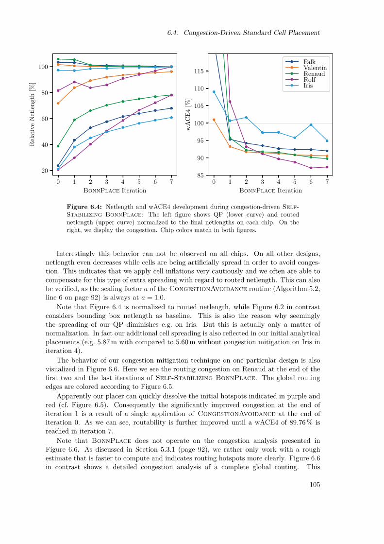
6.4. Congestion-Driven Standard Cell Placement
0 1 2 3 4 5 6 7BonnPlace Iteration
20
40
60
80
100
Rel
ativ
eN
etle
ngth
[%]
0 1 2 3 4 5 6 7BonnPlace Iteration
85
90
95
100
105
110
115
wA
CE4
[%]
FalkValentinRenaudRolfIris
Figure 6.4: Netlength and wACE4 development during congestion-driven Self-Stabilizing BonnPlace: The left figure shows QP (lower curve) and routednetlength (upper curve) normalized to the final netlengths on each chip. On theright, we display the congestion. Chip colors match in both figures.
Interestingly this behavior can not be observed on all chips. On all other designs,netlength even decreases while cells are being artificially spread in order to avoid conges-tion. This indicates that we apply cell inflations very cautiously and we often are able tocompensate for this type of extra spreading with regard to routed netlength. This can alsobe verified, as the scaling factor a of the CongestionAvoidance routine (Algorithm 5.2,line 6 on page 92) is always at a = 1.0.
Note that Figure 6.4 is normalized to routed netlength, while Figure 6.2 in contrastconsiders bounding box netlength as baseline. This is also the reason why seeminglythe spreading of our QP diminishes e.g. on Iris. But this is actually only a matter ofnormalization. In fact our additional cell spreading is also reflected in our initial analyticalplacements (e.g. 5.87 m with compared to 5.60 m without congestion mitigation on Iris initeration 4).
The behavior of our congestion mitigation technique on one particular design is alsovisualized in Figure 6.6. Here we see the routing congestion on Renaud at the end of thefirst two and the last iterations of Self-Stabilizing BonnPlace. The global routingedges are colored according to Figure 6.5.
Apparently our placer can quickly dissolve the initial hotspots indicated in purple andred (cf. Figure 6.5). Consequently the significantly improved congestion at the end ofiteration 1 is a result of a single application of CongestionAvoidance at the end ofiteration 0. As we can see, routability is further improved until a wACE4 of 89.76 % isreached in iteration 7.
Note that BonnPlace does not operate on the congestion analysis presented inFigure 6.6. As discussed in Section 5.3.1 (page 92), we rather only work with a roughestimate that is faster to compute and indicates routing hotspots more clearly. Figure 6.6in contrast shows a detailed congestion analysis of a complete global routing. This
105

Chapter 6. Experimental Results
0 30 50 60 70 76 82 87 91 95 100103 110
Figure 6.5: Legend for congestion visualizations; values in [%].
estimation is trustworthy and very accurate, but has only been computed for reasonsof comparison.
Even though this very instance Renaud is from the former 45 nm-node only, it has beena challenging test case for BonnPlace for many years. Previous versions of BonnPlace(Struzyna 2013) have not been capable of finding any placement which was even close toroutable. But with the proposed enhancements in Self-Stabilizing BonnPlace we cansolve this difficult instance well.
We demonstrated that BonnPlace is capable of effectively mitigating congestion onreal-world industrial designs.6.4.2 DAC 2012 Placement ContestIn this section we compare Self-Stabilizing BonnPlace to other state-of-the-art place-ment tools on the 2012 Design Automation Conference (DAC) placement contest bench-mark suite (Viswanathan et al. 2012).
All our placements are finally routed by the official contest router NCTUgr (Liu et al.2010; Liu, Li and Koh 2012) in regular mode with default parameters. Despite usingNCTUgr for a final estimation, we continue to consult BonnRouteGlobal (Müller,Radke and Vygen 2011) throughout our algorithm (cf. Section 5.3.1, page 92).
We compare the official contest metric, i.e. the scaled wirelength sWL defined as
sWL :=HPWL ·(
1 + 3100(RC− 100)
),
where RC := max100,wACE4 denotes the routing congestion. HPWL stands for the(unscaled) linear half-perimeter wiring length. We report the (scaled) wirelengths androuting congestion as determined by the official benchmark evaluation scripts.
All benchmarks were placed with identical parameter settings. We ran our placer witha target density of 90 % for four iterations. After each iteration, we updated our inflationslimiting the cell size increment to 50 % of the original cells’ size for each grid windowindividually.
Only for these benchmarks, we consider the bound-to-bound net model (B2B) with asuper-linear distance scaling factor for our analytical placements (cf. Struzyna 2013). Thissetup proved beneficial for these DAC benchmark designs, while on real-world instancesthe additional spreading due to quadratic netlength minimization is favorable – especiallyfor timing optimization. As of iteration one, we use the current placement to determinethe outer pins of nets for the B2B net model. Thus we do not have to run multiple QPswith B2B in order to stabilize the solution.
The results are summarized in Table 6.3. We compare ourselves to NTUPlace4 (Hsuet al. 2011), the best participant of the contest, and to the tool of Cong et al. (2013), whichachieved the best results on these benchmarks so far. We report the scaled wirelength(sWL) both as an absolute value and relative in [%] to the scaled wirelength produced byour Self-Stabilizing BonnPlace. Moreover for NTUPlace4 and our tool, we report
106

6.5. Timing-Driven Standard Cell Placement
(a) Iteration 0 (b) Iteration 1 (c) Iteration 7
Figure 6.6: Congestion on Renaud in the first two and the last iterations. Coloringaccording to Figure 6.5.
the routing congestion (RC). Note that the routing congestion of Cong et al. (2013) hasnot been published.
On average NTUPlace4 produces 4.04 % more scaled wirelength than our tool whilethe algorithm of Cong et al. (2013) produces 3.59 % more scaled wirelength. We get thebest published results on six out of the ten benchmark designs. Moreover we reduce therouting congestion RC on all chips attaining the minimum possible in eight out of tencases.
Our congestion mitigation technique is indeed very cautious; the scaling factor a (cf.Section 5.3) is consistently at a = 1.0. We inflate the movable cells’ area by 30.72 % onaverage. This increases HPWL by 3.84 % on average over the course of our iterations.In contrast to our experiments in Section 6.4, we here start with a higher target density,which is why a netlength increase due to congestion mitigation is expected. Despite of this,we are able to rapidly accomplish a drastically improved routability and hence optimizethis essential placement objective well.
It is not trivial to compare running times properly. The official benchmark wasperformed on 64−bit Intel Xeon CPU X7560 running at 2.27 GHz in single threaded mode.Our machine for these experiments is about 45 % faster and our placer is implemented torun highly parallel. In this setting, the former best placer by Cong et al. (2013) needed onaverage more than 225 % of our running time on eight threads. Our running time includesthe invocations of BonnRouteGlobal.
6.5 Timing-Driven Standard Cell PlacementNow we analyze the combined congestion-driven and timing-driven mode of Self-Stabilizing BonnPlace. In contrast to earlier versions of our placer (Brenner et al.2015), we will target both objectives at the same time.
Our timing-aware global placer introduced in Section 5.4 was run with default pa-rameters for timing optimization. These settings include the same congestion mitigationparameters as already discussed in Section 6.4. Furthermore we run 15 iterations intotal, where BonnLayerAssignment is applied from iteration 1 onward and BonnRe-finePlace is used starting with iteration 2.
107

Chapter 6. Experimental Results
Chip Self-StabilizingBonnPlace NTUPlace4Cong et al.
(2013)(Brenner et al. 2015) (Hsu et al. 2011)sWL RC Inf sWL sWL RC[×108] [%] [%] [×108] [%] [×108] [%] [%]
sb2 6.05 100.17 46.42 6.14 +1.49 6.24 +3.14 100.68sb3 3.22 100.00 58.03 3.60 +11.64 3.62 +12.26 103.53sb6 3.37 100.00 31.77 3.40 +0.81 3.42 +1.54 101.21sb7 4.07 100.00 19.23 3.95 −2.96 3.99 −2.10 100.68sb9 2.35 100.00 26.51 2.50 +6.31 2.55 +8.25 102.48sb11 3.44 100.02 15.97 3.40 −1.25 3.42 −0.62 100.02sb12 2.80 100.01 41.57 3.04 +8.38 3.12 +11.21 100.02sb14 2.26 100.00 15.53 2.45 +8.32 2.26 −0.26 100.07sb16 2.65 100.00 31.85 2.74 +3.38 2.80 +5.79 102.39sb19 1.51 100.00 20.30 1.51 −0.21 1.53 +1.18 100.61Avg 100.02 30.72 +3.59 +4.04 101.17
Table 6.3: Results of congestion-driven Self-Stabilizing BonnPlace on theDAC 2012 placement contest benchmark suite (Viswanathan et al. 2012). Wepresent the following metrics:
• sWL: Scaled wirelength (official contest metric)• RC: Routing congestion• Inf: Artificial cell inflation by our algorithm
All metrics are compared in [%] against BonnPlace. Improvements in green,marginal deviations in blue, degradations in red. Averages are the geometric meansof the ratios of the deviations.
In Table 6.4 we illustrate results obtained by Self-Stabilizing BonnPlace withthis configuration. We analyze four real-world designs from recent and older technologynodes.
To evaluate our approach we list multiple relevant metrics for each iteration: To beginwith, we specify the bounding box netlength NL in [m] as well as the routing congestionC measured in terms of wACE4 in [%]. For timing criteria we analyze worst slack WSin [ps] and the path-based FOM variant (abbreviated as FOM in Table 6.4) measured in[ps]. FOM is measured with respect to a slack target of 5 ps. All metrics were gatheredat the end of the respective iteration, after timing optimization on a legal placement.
The results show that over the course of iterations, we are able to improve timingbehavior significantly. From iteration 0 to 14 our placement flow reduces FOM by 97 %on average over the four chips. Using iteration 1 and 2 as baseline, we still improve FOMby 93 % and 72 % respectively. Also the worst slack SLK is considerably improved acrossall designs.
If we take a closer look at the results, we can justify the configuration of our flow: Afteriteration 0 we often face significant routing congestion, e.g. on Rolf or Falk. Similar tothe behavior analyzed in Section 6.4.1, considering one extra iteration with our congestionmitigation already significantly improves routability.
At the end of iteration 1 we perform BonnLayerAssignment for the first time.
108

6.5. Timing-Driven Standard Cell Placement
ItAug
ust
Rolf
Falk
Bene
dikt
NL
CSL
KFO
MNL
CSL
KFO
MNL
CSL
KFO
MNL
CSL
KFO
M[m
][%
][p
s][n
s][m
][%
][p
s][p
s][m
][%
][p
s][n
s][m
][%
][p
s][n
s]0
1.47
88.6
8−
368−
487
0.74
211.
60−
119
−71
532
1.34
122.
51−
126−
2127
9.06
90.8
8−
1090
−76
071
1.47
89.5
7−
257−
195
0.77
115.
78−
116−
2243
701.
2694.0
4−
42−
488
9.00
94.1
2−
470−
1254
21.
4989.2
2−
253−
179
0.80
117.
30−
18−
4579
1.32
94.3
3−
20−
174
9.05
91.0
3−
315
−78
73
1.48
90.5
5−
309−
201
0.83
110.
29−
18−
2852
1.30
93.0
9−
16−
127
9.00
89.8
2−
317
−83
04
1.48
90.7
4−
269−
194
0.83
102.
38−
11−
2463
1.29
91.5
8−
18−
122
8.94
89.2
3−
337
−85
65
1.48
91.0
1−
284−
189
0.83
99.3
5−
16−
6272
1.28
90.8
3−
17−
115
8.94
90.8
8−
341
−90
26
1.48
90.4
4−
263−
182
0.83
98.3
0−
12−
4400
1.26
92.0
7−
16−
988.
9191.3
7−
337
−90
37
1.47
90.3
6−
248−
179
0.84
98.4
9−
11−
2301
1.25
92.2
0−
15−
868.
8992.7
8−
345
−92
78
1.47
90.4
9−
259−
183
0.81
96.3
2−
8−
2147
1.25
92.3
1−
15−
558.
8789.6
7−
361
−96
49
1.47
91.3
2−
246−
175
0.79
95.1
6−
8−
2195
1.24
90.7
4−
13−
628.
8591.0
8−
309
−80
510
1.47
90.5
5−
245−
171
0.78
94.2
4−
12−
1835
1.25
93.8
2−
12−
468.
8491.3
7−
297
−76
111
1.48
90.4
5−
250−
180
0.77
94.3
3−
7−
1145
1.24
92.4
1−
13−
418.
8389.8
9−
299
−80
812
1.48
90.1
9−
252−
177
0.76
93.9
3−
9−
1319
1.24
92.6
9−
13−
368.
8290.3
5−
292
−75
413
1.48
90.0
1−
258−
178
0.76
93.6
2−
6−
192
1.24
92.4
0−
11−
338.
8391.1
5−
326
−87
014
1.48
89.9
7−
262−
181
0.76
93.4
1−
5−
165
1.23
92.6
5−
11−
308.
8190.7
0−
298
−72
8
Table6.4:
Tim
ing-driven
Self
-Sta
bili
zing
Bon
nPla
ceoverview
.Wepresentthefollo
wingmetric
son
Aug
ust,
Rolf,
Falk
and
Benedikt:
•NL:
Rou
tednetle
ngth
in[m
].•
C:R
outin
gcong
estio
nwACE4
in[%
].•
SLK:W
orst
slack
in[p
s].•
FOM:P
ath-ba
sedfig
ureof
merit
in[p
s],largevalues
in[n
s].
Allvalues
aremeasuredba
sedon
thelegalp
lacementat
theendof
each
ofthe
15ite
ratio
ns(It).
109

Chapter 6. Experimental Results
(a) Iteration 0 (b) Iteration 1 (c) Iteration 2 (d) Iteration 14
Figure 6.7: Timing-Driven Self-Stabilizing BonnPlace overview on Falk:We present the first three and the final iterations in the columns. The rows show:QP positions at the start of the iteration, congestion at the end of the iteration(coloring according to Figure 6.5) and cells in the legal placement colored by slack(most timing critical path highlighted).
This assignment of critical nets to fast layers significantly improves worst slack and FOMon all instances apart from Rolf. But on this instance timing degradations are only atemporary effect of our congestion mitigation, that we can shortly compensate. Startingwith iteration 2 we also incorporate BonnRefinePlace. Thus we especially improve theworst interconnections. This can be observed in terms of worst slack for example on Falkand Benedikt.
We also clearly observe that we target a wACE4 of 90 % as described in Section 5.3.2(page 93). Once we reach this goal, we do not reduce cell density further but at the sametime can preserve this wACE4.
Despite various additional steps in our timing-driven mode of Self-StabilizingBonnPlace, we more or less preserve the behavior visualized in Figure 6.4 with re-spect to routed netlength and wACE4. Particularly on Rolf where netlength increases inintermediate iterations, we can see that our balancing of opposing placement objectivesworks well.
Finally note that the version of Benedikt considered in Table 6.4 differs from the oneof Brenner et al. (2015). In the form at hand, Benedikt contains complicated paths whosegate delay is more than 120 % of the cycle time. Thus clearly negative slack can not beavoided here, even if all nets would have length 0. The variant of Brenner et al. (2015)re-optimized this logic to an extent where a worst slack of 0 ps was achievable.
The development of key metrics is exemplary depicted graphically in Figure 6.7 on
110

6.6. Mixed-Size Placement
Falk. We present visualizations of iterations 0, 1, 2 and 14 in the columns. In the first andsecond row we show the initial analytical placement and the congestion of the respectiveiteration (as e.g. in Figures 6.3 and 6.6).
In the last row, we show our final placement of each iteration where cells are coloredby slack and a critical path is highlighted in black. The coloring of slack is relative to thecycle time: More than 10 % slack compared to the cycle time is drawn in blue, positiveslack in green, less than 10 % negative slack relative to the cycle time is drawn in yellow,up to 25 % in orange and below this in purple. In each such visualization, we also add aworst path where respective endpoints are connected by thin black lines. Note that ourtiming optimizations start at the end of iteration 1, which is why we omit timing statisticsof the first iteration.
During the first two iterations we observe the behavior already discussed in Sections 6.3and 6.4.1 what QP spreading and congestion is concerned. In particular the vast majorityof critical routing problems can be resolved. Recall that we do not yet use BonnRe-finePlace at the end of iteration 1 which is why the critical path contains significantdetours.
At the end of iteration 2 we can observe two effects: On the one hand, new smallrouting hotspots arise (e.g. in the upper center). This is an effect of layer-assignmentwhich we can resolve over the course of subsequent iterations. On the other hand, timingcharacteristics of this placement apparently are much better. This can be observed globally(fewer orange cells) as well as locally with a straightened, shorter worst path.
After the final iteration almost all cells reach the slack target, or at least almost theslack target. Cells on the most critical path are placed so closely together that it is evenhard to spot this path connecting few orange boxes in the center of Falk. Note that thepurple boxes are clock buffers (LCBs) who only have incident clock nets hidden from thetiming environment. We achieve this placement while meeting the congestion targets.
We demonstrated that our Self-Stabilizing BonnPlace framework can balancedifferent placement objectives and is capable of finding routable placements with goodtiming characteristics on real-world designs.
6.6 Mixed-Size PlacementNow we present practical results of timing-driven BonnMacro. For this purpose weanalyze the quality of results in Section 6.6.1 before we specifically devote Section 6.6.2 torunning times both of MIP solving and the proposed overall timing-driven BonnMacroflow.6.6.1 Timing ResultsIn this section we analyze our timing-driven mixed-size placement approach. For thispurpose we particularly consider real-world instances where macro placement is relevantfor timing (cf. Table 6.1).
We consider all fairly large cells as macros. Note that this not necessarily includes allnon-standard cells, e.g. latches or clock buffers (LCBs) usually are only a few circuit rowshigh and thus not considered as macros in this section.
Results of this approach are presented in Table 6.5. For each chip, we compare threedifferent macro placements: First a baseline macro placement (base) used by our industrialpartner at some stage of the design process. It not necessarily describes the finallyproduced layout, but it is the latest state known to us. Such placements are createdmostly manually in many iterations by experienced designers.
111

Chapter 6. Experimental Results
Chip Run M-WS WS FOM NL[ps] [ps] [ns] [%] [m] [%]
Anna base −130 −272 −631 41.03BM −175 −272 −1 667 +164.22 39.74 −3.16BM TD −145 −298 −8 766 +1 289.24 67.78 +65.18
Rosemarie base −890 −957 −62 213 88.78BM −818 −818 −53 442 −14.10 74.87 −15.66BM TD −794 −893 −96 805 +55.60 227.19 +155.92
Sonja base −22 −22 −28 0.96BM −29 −30 −15 −45.44 0.93 −2.96BM TD −21 −21 −13 −54.15 0.93 −3.42
Anja base −56 −112 −59 34.49BM −109 −112 −58 −1.80 30.71 −10.95BM TD −29 −102 −16 −73.02 41.20 +19.46
Jannik base −105 −105 −557 4.61BM −126 −149 −871 +56.42 5.62 +21.89BM TD −89 −100 −683 +22.73 5.98 +29.78
Conni base −183 −255 −777 6.22BM −200 −245 −672 −13.55 4.73 −23.97BM TD −178 −183 −505 −34.97 6.51 +4.64
Lisa base −159 −174 −2 089 14.87BM −187 −201 −3 573 +71.03 19.45 +30.83BM TD −148 −154 −1 605 −23.19 24.69 +66.06
Benedikt base −181 −250 −480 7.14BM −181 −246 −487 +1.60 7.27 +1.86BM TD −210 −281 −572 +19.29 8.22 +15.12
Franziska base −36 −44 −56 9.65BM −28 −35 −17 −70.33 9.26 −4.04BM TD −14 −19 −8 −85.84 9.69 +0.38
Regina base −80 −125 −270 36.59BM −82 −102 −171 −36.80 35.09 −4.08BM TD −80 −105 −236 −12.59 36.29 −0.80
Mia base −62 −64 −50 24.53BM −53 −62 −30 −40.51 24.45 −0.32BM TD −71 −71 −42 −14.90 25.69 +4.74
Elias base −108 −248 −1 059 83.63BM −162 −248 −2 469 +133.11 84.14 +0.61BM TD −102 −248 −1 825 +72.30 89.05 +6.47
Table 6.5: Designer macro placement (base) compared with BonnMacro (BM)and timing-driven BonnMacro (BM TD). Columns denote:
• M-WS: Distance bound model worst slack in [ps].• WS: Actual worst slack in [ps] determined by timing engine.• FOM: Path-based figure of merit in [ns].• NL: Final bounding box netlength of legal placement in [m].
All metrics are compared against the baseline. Improvements in green, marginaldeviations in blue, degradations in red.
112

6.6. Mixed-Size Placement
The second macro placement compared (BM) is the result of standard (timing un-aware) BonnMacro. More precisely this includes a shredded placement of macros andsubsequent macro legalization. For each macro we try different packing modes (cf. Sec-tion 4.2) and solve each resulting local instance of Rectangle Packing with Spark(Funke 2011; Funke, Hougardy and Schneider 2016). The packing modes considered tothis end allow up to 3 unconstrained and 10 constrained macros, which empirically leadsto good solutions in terms of netlength. Such a legal placement is not post-optimized anyfurther.
Finally we also compare our timing-driven extension of BonnMacro (BM TD). Thisapproach has been described in Section 4.3 in great detail. It starts with the identicalshredded input placement as (timing unaware) BonnMacro, but models packing locallyas Timing-Driven Rectangle Packing instances.
During timing-driven macro legalization we consider two extra timing-driven packingmodes. For each such packing mode we solve a Timing-Driven Rectangle Packinginstance via a MIP-formulation (cf. Section 4.3.3). The first allows up to 5 unconstrainedand 20 constrained macros, up to 50 000 induced bounds for timing neighbors and a(deterministic) running time limit of roughly 2 min per MIP. The second mode in contrastrestricts these numbers to 4, 16, 25 000 and 30 s respectively. For each macro we selectthe first timing-driven legalization solution obtained within our running time limit. Incase both timing-driven packing modes time out, we fall back to a solution with minimummovement as determined by the aforementioned (timing unaware) packing modes.
We solve all MIPs with the barrier interior point method with multiple threads. Inorder to save running time, we solve MIPs with FOM and movement objective up to 0.5 %relative gap. Moreover we fix spatial relations of the FOM optimal solution for movementminimization.
Since timing-driven macro legalization can deviate further from the shredded inputplacement, the resulting macro placements can also be much denser. In order to compen-sate for this effect, we apply the whitespace post-optimization as discussed in Section 4.4.We use this algorithm to introduce small gaps of up to 4 circuit rows between macroswhile imposing minimal additional movement.
The quality of a macro placement can only be assessed based on a legal placementof the complete netlist. Therefore we evaluate all three macro placements in the sameway: We fix the macro positions and place the remaining cells legally using 5 iterations ofSelf-Stabilizing BonnPlace (cf. Section 5.2).
In order to analyze our timing model of distance bounds more directly, we disregardroutability. This allows to consider a more optimistic layer assignment matching underly-ing assumptions of our model. Thus we enable timing-optimization for Self-StabilizingBonnPlace in a special congestion-unaware mode and do not perform congestion miti-gation.
The resulting three legal placements for the entire netlist are compared in Table 6.5.We list the distance bound model worst slack M-WS in [ps] as well as the actual worst slackin [ps] as computed by the timing engine of IBM. In addition we show the actual path-based FOM, which we present in [ns] in order to simplify comparison of large numbers.Finally we also analyze the bounding box netlength of the placements in [m].
Before we discuss the difference in quality of the three placements, we note that ourimplementation of the distance bound model worst slack is optimistic in practice, i.e. anupper bound on the actual slack as shown in Proposition 3.3 (page 21). Given the various
113

Chapter 6. Experimental Results
sources of possible inaccuracies indicated in Figure 3.1, the distance bound slack correlatesfairly well with the actual slack.
Furthermore we observe that on all but 3 instances timing-driven BonnMacro(BM TD) finds the placements with best distance bound slacks. On Anna this macroplacement is only outperformed by the baseline. This design almost entirely consists ofmacros (highest macro density in Table 6.1). Recall that BonnMacro legalizes macroslocally in decreasing priority (cf. Section 4.2, page 50). This is why on this particularinstance, we have to pay some slack once small macros have to be packed between largeones with limited flexibility.
But the instances Benedikt and Mia require further explanations: Both have mediummacro density (cf. Table 6.1). Thus they particularly require macro positions betweenwhich standard cells can be placed easily in order to allow enough flexibility for subsequenttiming optimization. This requirement is only considered indirectly by BonnMacro asminimization of the deviation from the shredded input placement (in terms of movement).Timing unaware BonnMacro demonstrates that this type of movement objective isreasonable and therefore finds a placement with very competitive distance bound slack.
Timing-driven BonnMacro in contrast is encouraged to deviate from the input place-ment to maximize slack with respect to yet illegal standard cell positions (particularly forlatches). Later, once such macro positions are completed to legal placements of the entirenetlist, some detours can not be avoided. This is why the final latch positions are notoptimum with respect to distance bound slack. The same effect is also documented bycomparing the slack in our model directly after macro legalization (based on illegal stan-dard cell positions). Here these slacks have been much better (Benedikt: −129 ps, Mia:−37 ps). This overly optimistic evaluation explains the observed behavior on these twodesigns.
We refer to Section 6.6.3 for further ideas how to overcome both weaknesses in futureevolutions of timing-driven BonnMacro.
On the remaining instances, timing-driven BonnMacro not only consistently findspositions with best distance bound slack, but also outperforms both other placements interms of actual worst slack. While this is not surprising in comparison to (timing unaware)BonnMacro, it certainly was not expected relative to a hand-crafted baseline.
FOM is only considered as secondary objective by timing-driven BonnMacro. Nev-ertheless this approach finds significantly better placements in that regard on many in-stances. Most interestingly, this particularly again applies in comparison to the baseline.Moreover this holds for the great majority of instances, but particularly not for Annaand Rosemarie. These designs stand out, since both violate the premises of the distancebounds timing model (cf. Assumption 3.6; both contain non-endpoint macro-internal tim-ing nodes). Consequently the actual slack deviates a lot from the distance bound slack,which explains why FOM is not optimized well here.
In terms of netlength, Table 6.5 shows the expected trend: Regular BonnMacrotargets this objective well and outperforms the baseline on the majority of instances.Timing-driven BonnMacro on the other hand is expected to have higher netlength,since movement is only considered as third tie-breaker objective. The instances with themost drastic netlength increase are those with the highest macro densities. Here densermacro placements complicate placing standard logic, which is reflected in higher netlength.
The described effects are also visualized in Figure 6.8. Here the placements are coloredby the distance bounds slacks (cells without any bounds drawn in light gray). Moreoverwe can compare the most critical distance bounds in the baseline and timing-driven
114

6.6. Mixed-Size Placement
(a) Baseline Placement (b) Timing-Driven BonnMacro
Figure 6.8: Distance bound slacks on Lisa: Cells colored by slack. Overall criticalbounds drawn in black.
BonnMacro placements. Note that the respective critical bounds are not necessarilyidentical. These connections also overall define the actual worst slack. BonnMacro canimprove the overall critical connection as it aligns critical macros side by side (e.g. in theupper right of Figure 6.8(b)).
We demonstrated that BonnMacro can optimize various macro placement objectivesand particularly often computes solutions with very competitive worst slack. Such macroplacements not necessarily are perfect but can provide valuable guidance for designers.
6.6.2 Running TimeNow we analyze the running time of timing-driven macro placement. We first evaluatethe difference between various MIP formulations that have been proposed in Section 4.3.3,before we discuss running time contributions of various components of the proposed timing-driven macro placement flow.
Running Time of MIP SolvingInitially we compare the total time for solving different MIP formulations in Table 6.6.Therefore we analyze the deterministic solving times of CPLEX. This metric determinis-tically measures the computational effort of solving a MIP and does not depend on thecurrent load of the machine. This metric empirically correlates well with the actual wallclock time under benchmarking conditions.
115

Chapter 6. Experimental Results
Chip Run S F M[%] [%] [%]
Anna MA −99.37 −55.90 −72.05MA NL −99.87 −72.37 −93.12
Rosemarie MA −52.47 +6.56 −46.35MA NL −93.97 −66.53 −91.97
Sonja MA −68.02 +60.62 −3.55MA NL −47.14 −86.17 −64.27
Anja MA −43.26 −13.76 −1.60MA NL −12.79 −20.66 −49.19
Jannik MA −87.17 −85.92 −89.19MA NL −94.61 −95.20 −96.53
Conni MA −81.89 +42.75 −9.42MA NL −89.00 −62.53 −89.51
Lisa MA −45.05 −48.75 −48.95MA NL −49.67 +14.98 −61.44
Benedikt MA +2.30 +4.04 −53.09MA NL +14.23 −4.08 −53.99
Franziska MA −72.69 +12.16 −12.80MA NL −88.02 −92.66 −89.43
Regina MA −98.41 −98.88 −96.89MA NL −97.82 −99.60 −98.56
Mia MA −95.67 −93.58 −93.41MA NL −93.95 −97.51 −98.46
Elias MA −92.24 −82.06 −84.93MA NL −93.78 −94.36 −96.40
Summary MA −85.28 −61.65 −68.65MA NL −89.86 −85.56 −90.49
Table 6.6: Deterministic CPLEX running time comparison for solving MIPs withslack (S), FOM (F) and movement (M) objective. We show comparisons in [%] withthe baseline MIP formulation. MA stands for a formulation based on ManhattanArcs; MA NL in addition avoids extra variables for measuring bound lengths. Allcomparisons are summarized as geometric means of the ratios of the deviations.
116

6.6. Mixed-Size Placement
We compare three different MIP formulations for Timing-Driven Rectangle Pack-ing: As baseline we consider mixed-integer program 4.1 (page 63).
This baseline is compared with two different enhancements. Note that for technicalreasons we implemented improvements of Section 4.3.3 in reverse order they have beenpresented. The first variant (MA) exploits the geometry of Manhattan arcs. Similarlyto program 4.3 (page 65), this only requires 4 inequalities for any set of parallel distancebounds and one extra variable for the length of a bound. The second variant (MA NL)avoids this very variable (as already elaborated in program 4.2, page 64) and exactlydenotes mixed-integer program 4.3.
All versions use an identical timing-driven packing mode with different constants thanthose of Section 6.6.1 (no timeout, 3 unconstrained and 10 constrained rectangles, 30 000induced distance bounds). Note that we compare aggregated total deterministic CPLEXsolving running times of all MIPs considered throughout timing-driven BonnMacro. Dueto the nature of this algorithm, this not necessarily compares identical Timing-DrivenRectangle Packing instances. Nonetheless the results show a strong tendency.
Table 6.6 separately lists the times for solving the MIP with slack (S), FOM (F) andmovement (M) objectives. Note that we only show the relative running times comparedto the baseline in [%] since the actual absolute values are not very meaningful.
The comparisons in Table 6.6 very clearly show drastic running time improvements.Despite rare outliers, the overall time spent for CPLEX is significantly reduced on all chipsand for all objectives. The best MIP formulation MA NL reduces the MIP solving runningtime by more than 85 % on average for all objectives. Without these improvements moregenerous packing modes as used in Section 6.6.1 would not have been applicable.
Seemingly the majority of the running time improvement stems from exploiting Man-hattan arcs. But actually, both the baseline and MA optimized FOM-MIPs with fixedrelations only. This is not done in MA NL any longer, which is why improvements ofMA NL in FOM-MIPs particularly stand out. Moreover many instances that using MAbecame slower than the baseline, significantly speed up with MA NL.
In addition, the presented improvements do not only result from speeding up fewinstances with enormous running times. Also the maximum (deterministic CPLEX) timespent for solving single instances decreases almost identically as the totals presented inTable 6.6. This holds across all considered chips and objectives.
We also tried to solve our MIPs even faster by providing MIP starts for FOM andmovement MIPs. These can be inferred for the coordinate variables of rectangles fromthe previously solved programs. But this actually turned out to be harmful since CPLEXbecame slower with these initial assignments.
In summary, it therefore can be said that mixed-integer program 4.3 (Proposition 4.6,page 65) provides an essential improvement. This is why it has been used in all timing-driven BonnMacro experiments, particularly those discussed in the following section.Timing-Driven BonnMacro-FlowNow we analyze the running times of our proposed timing-driven macro placement flow.
Figure 6.9 visualizes the running times of different components in this flow. Theshown data refers to the BM TD runs of Table 6.5 on the same instances. We compareaccumulated total wall clock running times of these experiments.
Chronologically the first contribution is Self-Stabilizing BonnPlace with shreddedmacros denoted by BP (A). Recall that we run 3 iterations here using a special clusteringfor macro fragments.
117

Chapter 6. Experimental Results
Anna
Rosemarie
Sonja
Anja
Jannik
Conni
Lisa
Benedikt
Franziska
Regina
Mia
Elias
BP (A) BM CPX BP (B) BLA BRP
05:45:30
07:11:26
00:08:48
01:14:26
00:58:26
01:57:08
01:41:41
00:55:27
01:10:21
03:46:28
04:05:31
21:19:47
Figure 6.9: Running times of timing-driven BonnMacro components: Self-Stabilizing BonnPlace with shredded macros BP (A) and as evaluation withfixed macros BP (B), BonnMacro framework (BM) and MIP solving with CPLEX(CPX), timing optimizations BonnLayerAssignment (BLA) and BonnRefine-Place (BRP). Running time totals in [H:M:S].
Afterwards we display the contribution of the BonnMacro framework ( BM). Thisnot only accounts for the overhead of selecting local packing instances, but also in ourtiming-driven mode for library analysis, loading of distance bounds (Proposition 3.15)and construction of mixed-integer programs. The total time of solving these MIPs withCPLEX is summarized by CPX.
The resulting legal macro placement is afterwards considered as fixed. We evaluate tim-ing characteristics when this solution is extended to all standard cells. Therefore we per-form 5 iterations of timing-aware Self-Stabilizing BonnPlace denoted by BP (B).This step utilizes (congestion unaware) layer assignment using BonnLayerAssignment( BLA) as well as local placement changes using BonnRefinePlace ( BRP).
We summarize the respective total running times on the right of Figure 6.9 in [H:M:S].Figure 6.9 clearly shows that MIP solving consumes a significant amount of running
time during timing-driven BonnMacro. The classical (timing unaware) rectangle packingsolutions based on Spark (Funke, Hougardy and Schneider 2016) are also computed duringBM as additional alternatives. But this type of macro legalization runs so quickly thatit is even dominated by library analysis and distance bound loading in our timing drivenmode.
But apart from that the timing evaluation of a macro placement using Self-Stabilizing BonnPlace still dominates the running time on the majority of test cases.Even BonnLayerAssignment alone is more running time intensive than CPLEX on all
118

6.6. Mixed-Size Placement
but two designs. Even though CPLEX running time could likely be reduced slightly byfurther parameter tuning, this would not affect the overall running time significantly.
On the contrary we also explored larger packing instance parameters. Recall that weconsidered instances with up to 5 unconstrained, 20 constrained macros and up to 50 000distance bounds for the experiments presented so far. But as expected larger mixed-integerprograms hardly pay off: On the one hand, doubling the number of distance bounds on Miaincreases running time by 1293 %. On this instance CPLEX even fails to complete a firstcut-introducing phase within 1 hour of deterministic running time for 10 % of the packinginstances. On the other hand, considering up to 7 unconstrained and 30 constrainedmacros on Rosemarie results in 1644 % more running time.
The deterministic CPLEX time limit only is exceeded on 0.7 % of all Timing-DrivenRectangle Packing instances. In 92 % of these cases, we still find a satisfactory solutionand can continue: Either the next timing-driven packing mode with reduced constantssucceeds or the gap between the best known integer and fractional solutions is sufficientlysmall (below 5 %). For the most part the time limit is reached on FOM MIPs. Thisjustifies our choice of the timeout to avoid huge running times caused by few instances.
We demonstrated that our Timing-Driven Rectangle Packing instances are se-lected reasonably and considering larger constants can hardly be justified.
6.6.3 OutlookAt this point we want to indicate a few potential future extensions for BonnMacro. Allare inspired by current weaknesses and could help improve the quality of results.
A first issue is posed by relevant macro-internal non-endpoint timing nodes. Thosecan not be handled well using the model of slack based on distance bounds. Apportioningslack to paths before and after such nodes would be possible upfront, but likely requiresmany iterations until such estimates are reasonable everywhere.
On the other hand, small subsets of such nodes could be included into our formulationas mixed-integer program. For this purpose we could propagate arrival times directlywithin such a MIP similar to actual virtual timing. Such nodes could also be includedlazily and on demand once they become timing critical. Since arrival time propagationexpectedly is much more expensive than simply bounding distances with Manhattan arcs,such an extension must be used cautiously.
In order to improve the space management for standard logic, two approaches arepossible: On the one hand, we could optimize slack and FOM while restricting movementartificially (overall movement and/or individual movement of single macros). Consequentlymacro positions can deviate less from the shredded input positions which often leads toreduced detours and netlength (cf. timing unaware BonnMacro). On the other hand,such a restricted solution space might not be sufficient for optimizing timing properties.This could be compensated by iterating this approach with a new shredded placementguided by former iterations.
Furthermore logic could also be included in the macro legalization directly. Thereforewe could cluster standard cells into few large groups which could be respected in localpacking instances as rectangles with flexible aspect ratio. Similar approaches have alreadybeen applied for floorplanning (Adya and Markov 2003). Using excellent clusters, manydetours might be avoidable which should result in better netlength. At the same time suchan approach also provides the flexibility of incorporating a direct congestion mitigation intomacro placement. Therefore similar techniques as used in Self-Stabilizing BonnPlacecan be applied to the respective clusters.
119

Chapter 6. Experimental Results
Finally locally suboptimal solutions likely can be avoided by a post-optimization:Similar to the applied macro legalization, we simply could continue to solve local packinginstances. This might help improve the slack of smaller macros that are legalized at thevery last (as discussed on Anna). Such an approach requires a careful tradeoff betweenadditional running time and quality.
120

Summary
Placement is an important step in chip design, the process of finding physical layouts forelectronic computer chips. The basic task during placement is to arrange the buildingblocks of the chip, the circuits, disjointly within a given chip area. Since placementserves as baseline for multiple further optimizations, its quality has far reaching effects onthe overall solution. The main challenges in placement originate in requirements of thesubsequent design flow. This particularly includes finding positions that result in shortcircuit interconnections, that can be routed easily and that ensure all signals arrive intime. In this thesis we investigate various aspects of these challenges.
We mostly focus on the relatively few largest circuits on a chip, the macros. Due to thesize of macros, their placement pre-determines many characteristics of the chip. But atthe same time macro placement quality can hardly be assessed without placing all circuits.In order to still optimize timing, we propose a new timing model on macros which is basedon distance bounds. This model can be evaluated for positions of macros together withonly few extra cells. We prove that it bounds the worst slack that can be achieved byextending macro positions to all circuits. Yet it is accurate enough to predict these timingtraits under certain assumptions that are usually met in practice.
We show how this model can be computed efficiently and how equivalent but smallerrepresentations can be obtained. Packing rectangles disjointly remains strongly NP-hardunder slack maximization in our timing model. Despite of this we develop an algorithmthat solves special cases in O(nm) time where n and m denote the number of rectanglesand distance bounds.
The proposed timing model is also incorporated into BonnMacro. This is the macroplacement component of the placement framework BonnPlace developed at the ResearchInstitute for Discrete Mathematics of the University of Bonn. We extend the paradigm oflegalizing macros locally to optimize timing. Using efficient formulations as mixed-integerprograms relatively large local subinstances can be handled in practice in reasonable time.This results in the first timing-aware macro placement tool.
In addition, we provide multiple enhancements for the partitioning-based standardcell placer BonnPlaceGlobal of BonnPlace. We find a provably smallest model ofpartitioning as minimum-cost flow problem via reduction to a reachability problem ingraphs. Thus we can avoid running time intensive instances using an efficient sweep-linepre-processing and a thoughtful implementation. Moreover we propose the new globalplacement flow Self-Stabilizing BonnPlace. This approach combines partitioning-based BonnPlaceGlobal with a force-directed placement framework. It provides theflexibility to optimize the involved objectives routability and timing during placement.
The performance of our placement tools is confirmed on a large variety of real-worlddesigns provided by our industrial partner IBM. We reduce running time of Bonn-PlaceGlobal by up to 85 % on single instances and by 27 % on average on a large
121

Summary
testbed. Using Self-Stabilizing BonnPlace, we achieve the best published results onthe 2012 DAC congestion-driven placement contest (Viswanathan et al. 2012). Moreoverthis framework finds easily routable placements for challenging designs, even when simulta-neously optimizing timing objectives. Self-Stabilizing BonnPlace and timing-drivenBonnMacro can be combined to a mixed-size placement flow. This combination oftenfinds placements with a very competitive worst slack and even outperforms solutions thathave been determined manually by experienced designers.
122

Bibliography
G. M. Adelson-Velsky and E. M. Landis (1962). “An algorithm for the organization of information”.Trans. by J. R. Myron. In: Soviet Mathematics – Doklady 3, pp. 1259–1263 (cit. on p. 77).
S. N. Adya, S. Chaturvedi, J. A. Roy, D. A. Papa and I. L. Markov (2004). “Unification ofPartitioning, Placement and Floorplanning”. In: Proceedings of the 2004 International Con-ference on Computer-Aided Design. ICCAD (San Jose, California, USA), pp. 550–557. doi:10.1109/ICCAD.2004.1382639 (cit. on p. 12).
S. N. Adya and I. L. Markov (2003). “Fixed-outline Floorplanning: Enabling Hierarchical Design”.In: IEEE Transactions on Computer-Aided Design of Integrated Circuits and Systems 11.6,pp. 1120–1135. doi: 10.1109/TVLSI.2003.817546 (cit. on pp. 14, 119).
S. N. Adya and I. L. Markov (2005). “Combinatorial Techniques for Mixed-size Placement”. In:ACM Transactions on Design Automation of Electronic Systems 10.1, pp. 58–90. doi: 10.1145/1044111.1044116 (cit. on pp. 12, 48, 50).
S. N. Adya and X. Yang (2008). “Congestion-Driven Physical Design”. In: Handbook of Algorithmsfor Physical Design Automation. Ed. by C. J. Alpert, D. P. Mehta and S. S. Sapatnekar,pp. 447–466 (cit. on p. 17).
M. Ahrens, M. Gester, N. Klewinghaus, D. Müller, S. Peyer, C. Schulte and G. Téllez (2015).“Detailed Routing Algorithms for Advanced Technology Nodes”. In: IEEE Transactions onComputer-Aided Design of Integrated Circuits and Systems 34.4, pp. 563–576. doi: 10.1109/TCAD.2014.2385755 (cit. on p. 92).
C. J. Alpert, J. Hu, S. S. Sapatnekar and C. N. Sze (2006). “Accurate Estimation of Global BufferDelay Within a Floorplan”. In: IEEE Transactions on Computer-Aided Design of IntegratedCircuits and Systems 25.6, pp. 1140–1145. doi: 10.1109/TCAD.2005.855889 (cit. on p. 10).
C. J. Alpert, D. P. Mehta and S. S. Sapatnekar, eds. (2008). Handbook of Algorithms for PhysicalDesign Automation (cit. on pp. 8, 10, 16).
A. Armando, C. Castellini and E. Giunchiglia (1999–1999). “SAT-Based Procedures for TemporalReasoning”. In: Recent Advances in AI Planning. 5th European Conference on Planning. ECP(Durham, UK). Ed. by S. Biundo and M. Fox, pp. 97–108. doi: 10.1007/10720246_8 (cit. onp. 63).
R. Bayer (1972). “Symmetric Binary B-Trees: Data Structure and Maintenance Algorithms”. In:Acta Informatica 1.4, pp. 290–306. doi: 10.1007/BF00289509 (cit. on p. 77).
R. Bellman (1958). “On a routing problem”. In: Quarterly of Applied Mathematics (16), pp. 87–90.doi: 10.1090/qam/102435 (cit. on pp. 37, 38).
P. Berman and B. DasGupta (1992). “Approximating the rectilinear polygon cover problems”.In: Proceedings of the Fourth Canadian Conference on Computational Geometry (St. John’s,Newfoundland, Canada), pp. 229–235 (cit. on p. 59).
M. Bern and P. Plassmann (1989). “The Steiner problem with edge lengths 1 and 2”. In: Infor-mation Processing Letters 32.4, pp. 171–176. doi: 10.1016/0020-0190(89)90039-2 (cit. onp. 8).
123

Bibliography
A. Bock, S. Held, N. Kämmerling and U. Schorr (2015). “Local Search Algorithms for Timing-drivenPlacement Under Arbitrary Delay Models”. In: Proceedings of the 52nd Design AutomationConference. DAC (San Francisco, California, USA), Art. No. 29. doi: 10.1145/2744769.2744867 (cit. on p. 94).
A. Bock (2010). “Postoptimierung durch Umplatzierung und Gate Sizing”. Diploma Thesis. Re-search Institute for Discrete Mathematics, University of Bonn (cit. on p. 94).
A. Bortfeldt (2013). “A reduction approach for solving the rectangle packing area minimizationproblem”. In: European Journal of Operational Research 224.3, pp. 486–496. doi: 10.1016/j.ejor.2012.08.006 (cit. on p. 14).
U. Brenner (2007). An Effective Algorithm for Mixed-Size VLSI Placement. Technical Report 07970.Research Institute for Discrete Mathematics, University of Bonn (cit. on pp. 12, 47, 53).
U. Brenner (2012). “VLSI Legalization with Minimum Perturbation by Iterative Augmentation”.In: Proceedings of the 2012 Conference on Design, Automation and Test in Europe. DATE(Dresden, Germany), pp. 1385–1390. doi: 10.1109/DATE.2012.6176579 (cit. on pp. 89, 94).
U. Brenner, A. Hermann, N. Hoppmann and P. Ochsendorf (2015). “BonnPlace: A Self-StabilizingPlacement Framework”. In: Proceedings of the 2015 International Symposium on PhysicalDesign. ISPD (Monterey, California, USA), pp. 9–16. doi: 10.1145/2717764.2717778 (cit. onpp. 75, 76, 88, 95, 107, 108, 110).
U. Brenner and A. Rohe (2003). “An Effective Congestion-Driven Placement Framework”. In: IEEETransactions on Computer-Aided Design of Integrated Circuits and Systems 22.4, pp. 387–394.doi: 10.1109/TCAD.2003.809662 (cit. on pp. 16, 93).
U. Brenner, M. Struzyna and J. Vygen (2008). “BonnPlace: Placement of Leading-Edge Chips byAdvanced Combinatorial Algorithms”. In: IEEE Transactions on Computer-Aided Design ofIntegrated Circuits and Systems 27.9, pp. 1607–1620. doi: 10.1109/TCAD.2008.927674 (cit. onpp. 12, 16, 47, 75, 76, 89).
U. Brenner and J. Vygen (2001). “Worst-Case Ratios of Networks in the Rectilinear Plane”. In:Networks. An International Journal 38.3, pp. 126–139. doi: 10.1002/net.1031 (cit. on p. 89).
U. Brenner and J. Vygen (2008). “Analytical Methods in Placement”. In: Handbook of Algorithmsfor Physical Design Automation. Ed. by C. J. Alpert, D. P. Mehta and S. S. Sapatnekar,pp. 327–346 (cit. on p. 15).
M. Burstein and M. N. Youssef (1985). “Timing Influenced Layout Design”. In: Proceedings ofthe 22nd Design Automation Conference. DAC (Las Vegas, Nevada, USA), pp. 124–130. doi:10.1109/DAC.1985.1585923 (cit. on p. 17).
T. F. Chan, J. Cong, J. R. Shinnerl, K. Sze and M. Xie (2006). “mPL6: Enhanced Multilevel Mixed-Size Placement”. In: Proceedings of the 2006 International Symposium on Physical Design.ISPD (San Jose, California, USA), pp. 212–214. doi: 10.1145/1123008.1123055 (cit. onpp. 12, 16).
T. F. Chan, K. Sze, J. R. Shinnerl and M. Xie (2007). “mPL6: Enhanced Multilevel Mixed-Size Placement with Congestion Control”. In: Modern Circuit Placement: Best Practices andResults. Ed. by G.-J. Nam and J. Cong, pp. 247–288. doi: 10.1007/978-0-387-68739-1_10(cit. on pp. 12, 16).
Y.-C. Chang, Y.-W. Chang, G.-M. Wu and S.-W. Wu (2000). “B*-Trees: A New Representationfor Non-slicing Floorplans”. In: Proceedings of the 37th Design Automation Conference. DAC(Los Angeles, California, United States), pp. 458–463. doi: 10.1145/337292.337541 (cit. onp. 14).
T.-H. Chao, Y.-C. Hsu, J.-M. Ho, K. D. Boese and A. B. Kahng (1992). “Zero Skew Clock Routingwith Minimum Wirelength”. In: IEEE Transactions on Circuits and Systems II: Analog andDigital Signal Processing 39.11, pp. 799–814. doi: 10.1109/82.204128 (cit. on p. 39).
H. Chen, C.-K. Cheng, N.-C. Chou, A. B. Kahng, J. MacDonald, P. Suaris, B. Yao and Z. Zhu(2003). “An Algebraic Multigrid Solver for Analytical Placement with Layout Based Cluster-
124

Bibliography
ing”. In: Proceedings of the 40th Design Automation Conference. DAC (Anaheim, California,USA), pp. 794–799. doi: 10.1109/DAC.2003.1219127 (cit. on p. 16).
T.-C. Chen, Z.-W. Jiang, T.-C. Hsu, H.-C. Chen and Y.-W. Chang (2008). “NTUplace3: AnAnalytical Placer for Large-Scale Mixed-Size Designs With Preplaced Blocks and DensityConstraints”. In: IEEE Transactions on Computer-Aided Design of Integrated Circuits andSystems 27.7, pp. 1228–1240. doi: 10.1109/TCAD.2008.923063 (cit. on pp. 12, 17).
T.-C. Chen and Y.-W. Chang (2008). “Packing Floorplan Representations”. In: Handbook ofAlgorithms for Physical Design Automation. Ed. by C. J. Alpert, D. P. Mehta and S. S.Sapatnekar, pp. 203–238 (cit. on p. 14).
T.-C. Chen, P.-H. Yuh, Y.-W. Chang, F.-J. Huang and T.-Y. Liu (2008). “MP-Trees: A Packing-Based Macro Placement Algorithm for Modern Mixed-Size Designs”. In: IEEE Transactionson Computer-Aided Design of Integrated Circuits and Systems 27.9, pp. 1621–1634. doi: 10.1109/TCAD.2008.927760 (cit. on p. 14).
C.-L. E. Cheng (1994). “RISA: Accurate and Efficient Placement Routability Modeling”. In:Proceedings of the 1994 International Conference on Computer-Aided Design. ICCAD (SanJose, California, USA), pp. 690–695. doi: 10.1109/ICCAD.1994.629897 (cit. on p. 16).
J. Cong, L. Guojie, K. Tsota and X. Bingjun (2013). “Optimizing Routability in Large-ScaleMixed-Size Placement”. In: Proceedings of the 18th Asia and South Pacific Design AutomationConference. ASP-DAC (Yokohama, Japan), pp. 441–446. doi: 10.1109/ASPDAC.2013.6509636(cit. on pp. 106–108).
J. Cong, M. Romesis and J. R. Shinnerl (2005). “Robust Mixed-size Placement Under Tight White-space Constraints”. In: Proceedings of the 2005 International Conference on Computer-AidedDesign. ICCAD (San Jose, California, USA), pp. 165–172. doi: 10.1109/ICCAD.2005.1560058(cit. on p. 12).
J. C. Culberson and R. A. Reckhow (1988). “Covering Polygons is Hard”. In: Proceedings of the29th Annual Symposium on Foundations of Computer Science, pp. 601–611. doi: 10.1109/SFCS.1988.21976 (cit. on p. 59).
K. Doll, F. M. Johannes and K. J. Antreich (1994). “Iterative Placement Improvement by NetworkFlow Methods”. In: IEEE Transactions on Computer-Aided Design of Integrated Circuits andSystems 13.10, pp. 1189–1200. doi: 10.1109/43.317462 (cit. on pp. 12, 48).
A. E. Dunlop, V. D. Agrawal, D. N. Deutsch, M. F. Jukl, P. Kozak and M. Wiesel (1984).“Chip Layout Optimization Using Critical Path Weighting”. In: Proceedings of the 21st DesignAutomation Conference. DAC (Albuquerque, New Mexico, USA), pp. 133–136. doi: 10.1109/DAC.1984.1585786 (cit. on p. 17).
J. Edmonds and R. M. Karp (1972). “Theoretical Improvements in Algorithmic Efficiency forNetwork Flow Problems”. In: Journal of the ACM (JACM) 19.2, pp. 248–264. doi: 10.1145/321694.321699 (cit. on p. 89).
H. Eisenmann and F. M. Johannes (1998). “Generic Global Placement and Floorplanning”. In:Proceedings of the 35th Design Automation Conference. DAC (San Francisco, California, USA),pp. 269–274. doi: 10.1145/277044.277119 (cit. on pp. 12, 15, 17).
W. C. Elmore (1948). “The Transient Response of Damped Linear Networks with Particular Regardto Wideband Amplifiers”. In: Journal of Applied Physics 19.1, pp. 55–63. doi: 10.1063/1.1697872 (cit. on p. 9).
C. Engels (2013). “Algorithms for Macro Placement”. Master’s Thesis. Research Institute forDiscrete Mathematics, University of Bonn (cit. on pp. 50, 57, 58, 73).
P. Fernando and S. Katkoori (2008). “An Elitist Non-Dominated Sorting Based Genetic Algorithmfor Simultaneous Area and Wirelength Minimization in VLSI Floorplanning”. In: 21st Inter-national Conference on VLSI Design (Hyderabad, India), pp. 337–342. doi: 10.1109/VLSI.2008.97 (cit. on p. 14).
125

Bibliography
R. A. Finkel and J. L. Bentley (1974). “Quad Trees A Data Structure for Retrieval on CompositeKeys”. In: Acta Informatica 4.1, pp. 1–9. doi: 10.1007/BF00288933 (cit. on p. 78).
L. R. Ford (1956). Network Flow Theory. Tech. rep. P-923. Rand Corporation, Santa Monica (cit.on p. 37).
D. S. Franzblau (1989). “Performance Guarantees on a Sweep-Line Heuristic for Covering Rectilin-ear Polygons with Rectangles”. In: SIAM Journal on Discrete Mathematics 2.3, pp. 307–321.doi: 10.1137/0402027 (cit. on p. 59).
M. L. Fredman and R. E. Tarjan (1987). “Fibonacci Heaps and Their Uses in Improved NetworkOptimization Algorithms”. In: Journal of the ACM (JACM) 34.3, pp. 596–615. doi: 10.1145/28869.28874 (cit. on p. 33).
J. Funke (2011). “Netzlängenoptimale Platzierung von VLSI-Chips”. German. Diploma Thesis.Research Institute for Discrete Mathematics, University of Bonn (cit. on pp. 52, 58, 113).
J. Funke, S. Hougardy and J. Schneider (2016). “An Exact Algorithm for Wirelength OptimalPlacements in VLSI Design”. In: Integration. the VLSI Journal 52, pp. 355–366. doi: 10.1016/j.vlsi.2015.07.001 (cit. on pp. 14, 47, 52, 58, 63, 71, 113, 118).
T. Gao, P. M. Vaidya and C. L. Liu (1992). “A Performance Driven Macro-Cell PlacementAlgorithm”. In: Proceedings of the 29th Design Automation Conference (Anaheim, California,USA), pp. 147–152. doi: 10.1109/DAC.1992.227845 (cit. on p. 14).
M. R. Garey and D. S. Johnson (1975). “Complexity Results for Multiprocessor Scheduling underResource Constraints”. In: SIAM Journal on Computing 4, pp. 397–411. doi: 10.1137/0204035(cit. on pp. 25, 27).
M. R. Garey and D. S. Johnson (1978). ““Strong” NP-Completeness Results: Motivation, Exam-ples, and Implications”. In: Journal of the ACM (JACM) 25.3, pp. 499–508. doi: 10.1145/322077.322090 (cit. on p. 25).
M. Gester, D. Müller, T. Nieberg, C. Panten, C. Schulte and J. Vygen (2013). “BonnRoute:Algorithms and Data Structures for Fast and Good VLSI Routing”. In: ACM Transactions onDesign Automation of Electronic Systems 18.2, Art. No. 32. doi: 10.1145/2442087.2442103(cit. on pp. 8, 92).
A. V. Goldberg and A. V. Karzanov (2004). “Maximum skew-symmetric flows and matchings”. In:Mathematical Programming 100.3, pp. 537–568. doi: 10.1007/s10107-004-0505-z (cit. onp. 45).
L. J. Guibas and R. Sedgewick (1978). “A Dichromatic Framework for Balanced Trees”. In:Proceedings of the 19th Annual Symposium on Foundations of Computer Science. FOCS (AnnArbor, Michigan, USA), pp. 8–21. doi: 10.1109/SFCS.1978.3 (cit. on p. 77).
P.-N. Guo, C.-K. Cheng and T. Yoshimura (1999). “An O-Tree Representation of Non-SlicingFloorplan and Its Applications”. In: Proceedings of the 36th Design Automation Conference.DAC (New Orleans, Louisiana, United States), pp. 268–273. doi: 10.1109/DAC.1999.781324(cit. on p. 14).
T. Hamada, C.-K. Cheng and P. M. Chau (1993). “Prime: A Timing-driven Placement Tool Using aPiecewise Linear Resistive Network Approach”. In: Proceedings of the 30th Design AutomationConference. DAC (Dallas, Texas, USA), pp. 531–536. doi: 10.1145/157485.165015 (cit. onp. 17).
M. Hanan (1966). “On Steiner’s Problem with Rectilinear Distance”. In: SIAM Journal on AppliedMathematics 14.2, pp. 255–265. doi: 10.1137/0114025 (cit. on pp. 56, 78).
X. He, T. Huang, L. Xiao, H. Tian, G. Cui and E. F. Y. Young (2011). “Ripple: An EffectiveRoutability-driven Placer by Iterative Cell Movement”. In: Proceedings of the 2011 Interna-tional Conference on Computer-Aided Design. ICCAD (San Jose, California, USA), pp. 74–79.doi: 10.1109/ICCAD.2011.6105308 (cit. on p. 15).
126

Bibliography
M. R. Hestenes and E. Stiefel (1952). “Methods of conjugate gradients for solving linear systems”.In: Journal of Research of the National Institute of Standards and Technology 49.1, pp. 409–439(cit. on p. 75).
N. J. Higham (1993). “The Accuracy of Floating Point Summation”. In: SIAM Journal on ScientificComputing 14.4, pp. 783–799. doi: 10.1137/0914050 (cit. on p. 87).
R. B. Hitchcock, G. L. Smith and D. D. Cheng (1982). “Timing Analysis of Computer Hardware”.In: IBM Journal of Research and Development 26.1, pp. 100–105. doi: 10.1147/rd.261.0100(cit. on p. 9).
N. Hoppmann (2014). “Self-Stabilizing BonnPlace – A Self-Stabilizing Global Placement Frame-work”. Master’s Thesis. Research Institute for Discrete Mathematics, University of Bonn (cit.on pp. 90, 91).
W. Hou, H. Yu, X. Hong, Y. Cai, W. Wu, J. Gu and W. H. Kao (2001). “A New Congestion-Driven Placement Algorithm Based on Cell Inflation”. In: Proceedings of the 6th Asia andSouth Pacific Design Automation Conference. ASP-DAC (Yokohama, Japan), pp. 605–608.doi: 10.1145/370155.370560 (cit. on p. 16).
M.-K. Hsu, V. Balabanov and Y.-W. Chang (2013). “TSV-Aware Analytical Placement for 3-D ICDesigns Based on a Novel Weighted-Average Wirelength Model”. In: IEEE Transactions onComputer-Aided Design of Integrated Circuits and Systems 32.4, pp. 497–509. doi: 10.1109/TCAD.2012.2226584 (cit. on p. 15).
M.-K. Hsu, S. Chou, T.-H. Lin and Y.-W. Chang (2011). “Routability-driven Analytical Place-ment for Mixed-size Circuit Designs”. In: Proceedings of the 2011 International Conferenceon Computer-Aided Design. ICCAD (San Jose, California, USA), pp. 80–84. doi: 10.1109/ICCAD.2011.6105309 (cit. on pp. 16, 17, 106, 108).
B. Hu and M. Marek-Sadowska (2005). “Multilevel Fixed-Point-Addition-Based VLSI Placement”.In: IEEE Transactions on Computer-Aided Design of Integrated Circuits and Systems 24.8,pp. 1188–1203. doi: 10.1109/TCAD.2005.850802 (cit. on p. 16).
J. Hu, J. A. Roy and I. L. Markov (2010). “Completing High-quality Global Routes”. In: Proceedingsof the 2010 International Symposium on Physical Design. ISPD (San Francisco, California,USA), pp. 35–41. doi: 10.1145/1735023.1735035 (cit. on p. 16).
M. A. B. Jackson and E. S. Kuh (1989). “Performance-driven Placement of Cell Based IC’s”.In: Proceedings of the 26th Design Automation Conference. DAC (Las Vegas, Nevada, USA),pp. 370–375. doi: 10.1145/74382.74444 (cit. on p. 17).
A. Janiak, A. Kozik and M. Lichtenstein (2010). “New perspectives in VLSI design automation:deterministic packing by Sequence Pair”. In: Annals of Operations Research 179.1, pp. 35–56.doi: 10.1007/s10479-008-0460-9 (cit. on p. 14).
M. Jerrum (1985). Complementary Partial Orders and Rectangle Packing. Tech. rep. CSR-190-85.University of Edinburgh, Department of Computer Science. 10 pp. (cit. on p. 14).
W. Kahan (1965). “Further Remarks on Reducing Truncation Errors”. In: Communications of theACM 8.1, p. 40. doi: 10.1145/363707.363723 (cit. on p. 87).
A. B. Kahng and Q. Wang (2005). “Implementation and Extensibility of an Analytic Placer”.In: IEEE Transactions on Computer-Aided Design of Integrated Circuits and Systems 24.5,pp. 734–747. doi: 10.1109/TCAD.2005.846366 (cit. on pp. 12, 16).
R. M. Karp (1972). “Reducibility Among Combinatorial Problems”. In: Complexity of ComputerComputations. The IBM Research Symposia Series, pp. 85–103. doi: 10.1007/978-1-4684-2001-2_9 (cit. on pp. 8, 25).
R. M. Karp (1978). “A characterization of the minimum cycle mean in a digraph”. In: DiscreteMathematics 23.3, pp. 309–311. doi: 10.1016/0012-365X(78)90011-0 (cit. on pp. 32, 37).
R. M. Karp and J. B. Orlin (1981). “Parametric shortest path algorithms with an applicationto cyclic staffing”. In: Discrete Applied Mathematics 3.1, pp. 37–45. doi: 10.1016/0166-218X(81)90026-3 (cit. on p. 33).
127

Bibliography
A. Khatkhate, C. Li, A. R. Agnihotri, M. C. Yildiz, S. Ono, C.-K. Koh and P. H. Madden (2004).“Recursive Bisection Based Mixed Block Placement”. In: Proceedings of the 2004 InternationalSymposium on Physical Design (Phoenix, Arizona, USA), pp. 84–89. doi: 10.1145/981066.981084 (cit. on p. 12).
M.-C. Kim, N. Viswanathan, C. J. Alpert, I. Markov and S. Ramji (2012). “MAPLE: Multi-level Adaptive PLacEment for Mixed-Size Designs”. In: Proceedings of the 2012 InternationalSymposium on Physical Design. ISPD (Napa, California, USA), pp. 193–200. doi: 10.1145/2160916.2160958 (cit. on pp. 12, 15).
M.-C. Kim, J. Hu, D.-J. Lee and I. Markov (2011). “A SimPLR Method for Routability-drivenPlacement”. In: Proceedings of the 2011 International Conference on Computer-Aided Design.ICCAD (San Jose, California, USA), pp. 67–73. doi: 10.1109/ICCAD.2011.6105307 (cit. onpp. 15, 16).
M.-C. Kim, D.-J. Lee and I. L. Markov (2012). “SimPL: An Effective Placement Algorithm”. In:IEEE Transactions on Computer-Aided Design of Integrated Circuits and Systems 31.1, pp. 50–60. doi: 10.1109/TCAD.2011.2170567 (cit. on pp. 15, 16, 89, 103).
M.-C. Kim, D.-J. Lee and I. L. Markov (2013). “SimPL: An Algorithm for Placing VLSI Circuits”.In: Communications of the ACM 56.6, pp. 105–113. doi: 10.1145/2461256.2461279 (cit. onpp. 15, 89, 103).
M.-C. Kim and I. L. Markov (2012). “ComPLx: A Competitive Primal-dual Lagrange Optimizationfor Global Placement”. In: Proceedings of the 49th Design Automation Conference. DAC (SanFrancisco, California, USA), pp. 747–752. doi: 10.1145/2228360.2228496 (cit. on pp. 12, 15).
T. I. Kirkpatrick and N. R. Clark (1966). “Pert as an Aid to Logic Design”. In: IBM Journal ofResearch and Development 10.2, pp. 135–141. doi: 10.1147/rd.102.0135 (cit. on p. 9).
J. M. Kleinhans, G. Sigl, F. M. Johannes and K. J. Antreich (1991). “GORDIAN: VLSI Placementby Quadratic Programming and Slicing Optimization”. In: IEEE Transactions on Computer-Aided Design of Integrated Circuits and Systems 10.3, pp. 356–365. doi: 10.1109/43.67789(cit. on p. 15).
W. Kocay and D. Stone (1993). “Balanced network flows”. In: Bulletin of the Institute of Combi-natorics and its Applications 7, pp. 17–32 (cit. on p. 45).
W. Kocay and D. Stone (1995). “An Algorithm for Balanced Flows”. In: Journal of CombinatorialMathematics and Combinatorial Computing 19, pp. 3–32 (cit. on p. 45).
T. Kong (2002). “A Novel Net Weighting Algorithm for Timing-driven Placement”. In: Proceedingsof the 2002 International Conference on Computer-Aided Design. ICCAD (San Jose, California,USA), pp. 172–176. doi: 10.1145/774572.774597 (cit. on p. 17).
R. E. Korf, M. D. Moffitt and M. E. Pollack (2010). “Optimal rectangle packing”. In: Annals ofOperations Research 179.1, pp. 261–295. doi: 10.1007/s10479-008-0463-6 (cit. on pp. 14,63).
B. H. Korte and J. Vygen (2018). Combinatorial Optimization. Theory and Algorithms. 6th ed.Vol. 21. 698 pp. doi: 10.1007/978-3-662-56039-6 (cit. on pp. 4, 22).
B. Korte, D. Rautenbach and J. Vygen (2007). “BonnTools: Mathematical Innovation for Layoutand Timing Closure of Systems on a Chip”. In: Proceedings of the IEEE 95.3, pp. 555–572.doi: 10.1109/JPROC.2006.889373 (cit. on pp. 1, 75, 88).
H. W. Lenstra (1983). “Integer Programming with a Fixed Number of Variables”. In: Mathematicsof Operations Research 8.4, pp. 538–548. doi: 10.1287/moor.8.4.538 (cit. on p. 72).
Z. Li, D. A. Papa, C. J. Alpert, S. Hu, W. Shi, C. Sze and Y. Zhou (2010). “Ultra-Fast InterconnectDriven Cell Cloning For Minimizing Critical Path Delay”. In: Proceedings of the 2010 Interna-tional Symposium on Physical Design. ISPD (San Francisco, California, USA), pp. 75–82. doi:10.1145/1735023.1735047 (cit. on p. 39).
128

Bibliography
J.-M. Lin and Y.-W. Chang (2005). “TCG: A Transitive Closure Graph-Based Representation forGeneral Floorplans”. In: IEEE Transactions on Very Large Scale Integration (VLSI) Systems13.2, pp. 288–292. doi: 10.1109/TVLSI.2004.840760 (cit. on p. 14).
J.-M. Lin, Y.-W. Chang and S.-P. Lin (2003). “Corner Sequence - A P-Admissible FloorplanRepresentation With a Worst Case Linear-Time Packing Scheme”. In: IEEE Transactions onVery Large Scale Integration (VLSI) Systems 11.4, pp. 679–686. doi: 10.1109/TVLSI.2003.816137 (cit. on p. 14).
T. Lin and C. Chu (2014). “POLAR 2.0: An Effective Routability-Driven Placer”. In: Proceedingsof the 51nd Design Automation Conference. DAC (San Francisco, California, USA), Art. No.123. doi: 10.1145/2593069.2593181 (cit. on pp. 15, 17).
T. Lin, C. Chu, J. R. Shinnerl, I. Bustany and I. Nedelchev (2015). “POLAR: A High PerformanceMixed-Size Wirelengh-Driven Placer With Density Constraints”. In: IEEE Transactions onComputer-Aided Design of Integrated Circuits and Systems 34.3, pp. 447–459. doi: 10.1109/TCAD.2015.2394383 (cit. on p. 15).
F. Liu and P. Feldmann (2008–2008). “MAISE: An Interconnect Simulation Engine for Timingand Noise Analysis”. In: 9th International Symposium on Quality Electronic Design. ISQED(San Jose, California, USA), pp. 621–626. doi: 10.1109/ISQED.2008.4479809 (cit. on p. 10).
W.-H. Liu, W.-C. Kao, Y.-L. Li and K.-Y. Chao (2010). “Multi-threaded Collision-aware GlobalRouting with Bounded-length Maze Routing”. In: Proceedings of the 47th Design AutomationConference. DAC (Anaheim, California, USA), pp. 200–205. doi: 10.1145/1837274.1837324(cit. on p. 106).
W.-H. Liu, Y.-L. Li and C.-K. Koh (2012). “A Fast Maze-free Routing Congestion Estimator withHybrid Unilateral Monotonic Routing”. In: Proceedings of the 2012 International Conferenceon Computer-Aided Design. ICCAD (San Jose, California, USA), pp. 713–719 (cit. on p. 106).
J. Lu, H. Zhuang, P. Chen, H. Chang, C. Chang, Y. Wong, L. Sha, D. Huang, Y. Luo, C. Tengand C. Cheng (2015). “ePlace-MS: Electrostatics-Based Placement for Mixed-Size Circuits”.In: IEEE Transactions on Computer-Aided Design of Integrated Circuits and Systems 34.5,pp. 685–698. doi: 10.1109/TCAD.2015.2391263 (cit. on pp. 12, 16).
J. Lu, P. Chen, C.-C. Chang, L. Sha, D. J.-H. Huang, C.-C. Teng and C.-K. Cheng (2015). “ePlace:Electrostatics-Based Placement Using Fast Fourier Transform and Nesterov’s Method”. In:ACM Transactions on Design Automation of Electronic Systems 20.2, Art. No. 17. doi: 10.1145/2699873 (cit. on pp. 12, 16, 89).
T. Luo, D. Newmark and D. Z. Pan (2006). “A New LP Based Incremental Timing DrivenPlacement for High Performance Designs”. In: Proceedings of the 43rd Design AutomationConference. DAC, pp. 1115–1120. doi: 10.1145/1146909.1147190 (cit. on p. 17).
I. L. Markov, J. Hu and M.-C. Kim (2015). “Progress and Challenges in VLSI Placement Research”.In: Proceedings of the IEEE 103.11, pp. 1985–2003. doi: 10.1109/JPROC.2015.2478963 (cit.on pp. 16, 17).
N. Megiddo (1983). “Applying Parallel Computation Algorithms in the Design of Serial Algo-rithms”. In: Journal of the ACM (JACM) 30.4, pp. 852–865. doi: 10.1145/2157.322410(cit. on p. 33).
F. Michaelis (2015). “Verbesserungen von Algorithmen für die Platzierung von Macros”. German.Bachelor’s Thesis. Research Institute for Discrete Mathematics, University of Bonn (cit. onpp. 53, 58).
M. D. Moffitt, A. N. Ng, I. L. Markov and M. E. Pollack (2006). “Constraint-Driven FloorplanRepair”. In: Proceedings of the 43rd Design Automation Conference. DAC, pp. 1103–1108. doi:10.1145/1146909.1147188 (cit. on p. 14).
E. F. Moore (1959). “The shortest path through a maze”. In: Proceedings of the InternationalSymposium on Switching Theory. Vol. II, pp. 285–292 (cit. on p. 37).
129
Bibliography
D. Müller, K. Radke and J. Vygen (2011). “Faster Min–Max Resource Sharing in Theory andPractice”. In: Mathematical Programming Computation 3.1, pp. 1–35. doi: 10.1007/s12532-011-0023-y (cit. on pp. 17, 92, 106).
H. Murata, K. Fujiyoshi, S. Nakatake and Y. Kajitani (1996). “VLSI Module Placement Based onRectangle-Packing by the Sequence-Pair”. In: IEEE Transactions on Computer-Aided Designof Integrated Circuits and Systems 15.12, pp. 1518–1524. doi: 10.1109/43.552084 (cit. onp. 14).
S. Nakatake, K. Fujiyoshi, H. Murata and Y. Kajitani (1996). “Module Placement on BSG-structure and IC Layout Applications”. In: Proceedings of the 1996 International Conferenceon Computer-Aided Design, pp. 484–491. doi: 10.1109/ICCAD.1996.569870 (cit. on p. 14).
G.-J. Nam (2006). “ISPD 2006 Placement Contest: Benchmark Suite and Results”. In: Proceedingsof the 2006 International Symposium on Physical Design. ISPD (San Jose, California, USA),pp. 167–167. doi: 10.1145/1123008.1123042 (cit. on p. 7).
G.-J. Nam, C. J. Alpert, P. Villarrubia, B. Winter and M. Yildiz (2005). “The ISPD 2005 Place-ment Contest and Benchmark Suite”. In: Proceedings of the 2005 International Symposium onPhysical Design. ISPD (San Francisco, California, USA), pp. 216–220. doi: 10.1145/1055137.1055182 (cit. on p. 7).
G.-J. Nam and J. Cong, eds. (2007). Modern Circuit Placement: Best Practices and Results. doi:10.1007/978-0-387-68739-1_10 (cit. on p. 16).
W. Naylor, R. Donelly and L. Sha (2001). “Non-linear optimization system and method for wirelength and delay optimization for an automatic electric circuit placer”. US6301693B1 (cit. onpp. 15, 16).
H. Onodera, Y. Taniguchi and K. Tamaru (1991). “Branch-and-bound Placement for BuildingBlock Layout”. In: Proceedings of the 28th Design Automation Conference (San Francisco,California, USA), pp. 433–439. doi: 10.1145/127601.127708 (cit. on p. 14).
R. H. J. M. Otten (1998). “Global Wires: Harmful?” In: Proceedings of the 1998 InternationalSymposium on Physical Design. ISPD (Monterey, California, USA), pp. 104–109. doi: 10.1145/274535.274550 (cit. on pp. 9, 10).
D. Z. Pan, B. Halpin and H. Ren (2008). “Timing-Driven Placement”. In: Handbook of Algorithmsfor Physical Design Automation. Ed. by C. J. Alpert, D. P. Mehta and S. S. Sapatnekar,pp. 423–446 (cit. on p. 17).
C. L. Ratzlaff and L. T. Pillage (1994). “RICE: Rapid Interconnect Circuit Evaluation UsingAWE”. In: IEEE Transactions on Computer-Aided Design of Integrated Circuits and Systems13.6, pp. 763–776. doi: 10.1109/43.285250 (cit. on p. 10).
J. A. Roy, S. N. Adya, D. A. Papa and I. L. Markov (2006). “Min-Cut Floorplacement”. In: IEEETransactions on Computer-Aided Design of Integrated Circuits and Systems 25.7, pp. 1313–1326. doi: 10.1109/TCAD.2005.855969 (cit. on pp. 12, 16, 17).
J. A. Roy and I. L. Markov (2007). “Seeing the Forest and the Trees: Steiner Wirelength Optimiza-tion in Placement”. In: IEEE Transactions on Computer-Aided Design of Integrated Circuitsand Systems 26.4, pp. 632–644. doi: 10.1109/TCAD.2006.888260 (cit. on p. 17).
S. S. Sapatnekar (2004). Timing (cit. on p. 10).H. E. Scarf (1981a). “Production Sets with Indivisibilities, Part I: Generalities”. In: Econometrica
49.1, pp. 1–32. doi: 10.2307/1911124 (cit. on p. 72).H. E. Scarf (1981b). “Production Sets with Indivisibilities, Part II: The Case of Two Activities”.
In: Econometrica 49.2, pp. 395–423. doi: 10.2307/1913318 (cit. on p. 72).J. Schneider (2009). “Macro Placement in VLSI-Design”. Diploma Thesis. Research Institute for
Discrete Mathematics, University of Bonn (cit. on pp. 47, 55, 57).D. Shmoys and É. Tardos (1993). “An approximation algorithm for the generalized assignment
problem”. In: Mathematical Programming 62, pp. 461–474. doi: 10.1007/BF01585178 (cit. onp. 76).
130

Bibliography
J. Silvanus and J. Vygen (2017). Few Sequence Pairs Suffice. Representing All Rectangle Place-ments. arXiv: 1708.09779 [math.CO] (cit. on p. 14).
P. Spindler, U. Schlichtmann and F. M. Johannes (2008). “Kraftwerk2 – A Fast Force-DirectedQuadratic Placement Approach Using an Accurate Net Model”. In: IEEE Transactions onComputer-Aided Design of Integrated Circuits and Systems 27.8, pp. 1398–1411. doi: 10 .1109/TCAD.2008.925783 (cit. on pp. 12, 15, 76).
A. Srinivasan, K. Chaudhary and E. S. Kuh (1992). “RITUAL: A Performance Driven PlacementAlgorithm”. In: IEEE Transactions on Circuits and Systems II: Analog and Digital SignalProcessing 39.11, pp. 825–840. doi: 10.1109/82.204130 (cit. on p. 17).
M. Struzyna (2010). “Flow-based Partitioning and Fast Global Placement in Chip Design”. Dis-sertation. Research Institute for Discrete Mathematics, University of Bonn (cit. on p. 77).
M. Struzyna (2011). “Flow-based partitioning and position constraints in VLSI placement”. In: Pro-ceedings of the 2011 Conference on Design, Automation and Test in Europe. DATE (Grenoble,France), pp. 1–6. doi: 10.1109/DATE.2011.5763100 (cit. on pp. 75–79, 81, 89, 99).
M. Struzyna (2013). “Sub-Quadratic Objectives in Quadratic Placement”. In: Proceedings of the2013 Conference on Design, Automation and Test in Europe. DATE (Grenoble, France),pp. 1867–1872. doi: 10.7873/DATE.2013.372 (cit. on pp. 16, 75, 76, 89, 106).
T.-Y. Sun, S.-T. Hsieh, H.-M. Wang and C.-W. Lin (2006). “Floorplanning based on Particle SwarmOptimization”. In: Proceedings of the 2006 Annual Symposium on Emerging VLSI Technologiesand Architectures. ISVLSI (Karlsruhe, Germany), pp. 7–11. doi: 10.1109/ISVLSI.2006.46(cit. on p. 14).
S. Sutanthavibul, E. Shragowitz and J. B. Rosen (1990). “An Analytical Approach to Floorplan De-sign and Optimization”. In: Proceedings of the 27th Design Automation Conference (Orlando,Florida, USA), pp. 187–192. doi: 10.1145/123186.123255 (cit. on p. 62).
C. Szegedy (2005). “Some Applications of the Weighted Combinatorial Laplacian”. Dissertation.Research Institute for Discrete Mathematics, University of Bonn (cit. on p. 17).
T. Takahashi (2000). “A New Encoding Scheme for Rectangle Packing Problem”. In: Proceedingsof the 37th Design Automation Conference. DAC (Los Angeles, California, United States),pp. 175–178. doi: 10.1109/ASPDAC.2000.835091 (cit. on p. 14).
M. Tang and A. Sebastian (2005). “A Genetic Algorithm for VLSI Floorplanning Using O-TreeRepresentation”. In: Applications of Evolutionary Computing. Proceedings of the EvoWorkshops2005. Ed. by F. Rothlauf, J. Branke, S. Cagnoni, D. W. Corne, R. Drechsler, Y. Jin, P. Machado,E. Marchiori, J. Romero, G. D. Smith and G. Squillero, pp. 215–224. doi: 10.1007/978-3-540-32003-6_22 (cit. on p. 14).
R. E. Tarjan (1975). “Efficiency of a Good But Not Linear Set Union Algorithm”. In: Journal ofthe ACM (JACM) 22.2, pp. 215–225. doi: 10.1145/321879.321884 (cit. on p. 84).
N. Tomizawa (1971). “On Some Techniques Useful for Solution of Transportation NetworkProblems”. In: Networks. An International Journal 1.2, pp. 173–194. doi: 10.1002/net.3230010206 (cit. on p. 89).
N. Viswanathan, C. J. Alpert, C. Sze, Z. Li and Y. Wei (2012). “The DAC 2012 Routability-DrivenPlacement Contest and Benchmark Suite”. In: Proceedings of the 49th Design AutomationConference. DAC (San Francisco, California, USA), pp. 774–782. doi: 10.1145/2228360.2228500 (cit. on pp. 103, 106, 108, 122).
N. Viswanathan, G.-J. Nam, C. J. Alpert, P. G. Villarrubia, H. Ren and C. Chu (2007). “RQL:Global Placement via Relaxed Quadratic Spreading and Linearization”. In: Proceedings of the44th Design Automation Conference. DAC (San Diego, California, USA), pp. 453–458. doi:10.1145/1278480.1278599 (cit. on p. 15).
N. Viswanathan, M. Pan and C. Chu (2006). “FastPlace 2.0: An Efficient Analytical Placer forMixed-mode Designs”. In: Proceedings of the 11th Asia and South Pacific Design Automation
131

Bibliography
Conference. ASP-DAC (Yokohama, Japan), pp. 195–200. doi: 10.1145/1118299.1118354(cit. on pp. 12, 15).
N. Viswanathan, M. Pan and C. Chu (2007). “FastPlace 3.0: A Fast Multilevel Quadratic PlacementAlgorithm with Placement Congestion Control”. In: Proceedings of the 12th Asia and SouthPacific Design Automation Conference. ASP-DAC (Yokohama, Japan), pp. 135–140. doi: 10.1109/ASPDAC.2007.357975 (cit. on pp. 12, 15, 16).
C. Visweswariah, K. Ravindran, K. Kalafala, S. G. Walker, S. Narayan, D. K. Beece, J. Piaget, N.Venkateswaran and J. G. Hemmett (2006). “First-Order Incremental Block-Based StatisticalTiming Analysis”. In: IEEE Transactions on Computer-Aided Design of Integrated Circuitsand Systems 25.10, pp. 2170–2180. doi: 10.1109/TCAD.2005.862751 (cit. on p. 10).
J. Vygen (2005). “Geometric quadrisection in linear time, with application to VLSI placement”.In: Discrete Optimization 2.4, pp. 362–390. doi: 10.1016/j.disopt.2005.08.007 (cit. onp. 76).
Y. Wei, C. Sze, N. Viswanathan, Z. Li, C. J. Alpert, L. Reddy, A. D. Huber, G. E. Tellez, D.Keller and S. S. Sapatnekar (2012). “GLARE: Global and Local Wiring Aware RoutabilityEvaluation”. In: Proceedings of the 49th Design Automation Conference. DAC (San Francisco,California, USA), pp. 768–773. doi: 10.1145/2228360.2228499 (cit. on p. 104).
D. M. Wochnik (2017). “Verbesserte Algorithmen für die Platzierung von Makros”. Master’s Thesis.Research Institute for Discrete Mathematics, University of Bonn (cit. on pp. 56, 59, 73).
G. Wu and C. Chu (2017). “Two Approaches for Timing-Driven Placement by Lagrangian Relax-ation”. In: IEEE Transactions on Computer-Aided Design of Integrated Circuits and Systems36.12, pp. 2093–2105. doi: 10.1109/TCAD.2017.2697947 (cit. on p. 17).
Z. Xiu and R. Rutenbar (2007). “Mixed-Size Placement with Fixed Macrocells using Grid-Warping”. In: Proceedings of the 2007 International Symposium on Physical Design. ISPD(Austin, Texas, USA), pp. 103–110. doi: 10.1145/1231996.1232019 (cit. on p. 16).
Y. Xu, Y. Zhang and C. Chu (2009). “FastRoute 4.0: Global Router with Efficient via Mini-mization”. In: Proceedings of the 14th Asia and South Pacific Design Automation Conference.ASP-DAC (Yokohama, Japan), pp. 576–581. doi: 10.1145/1509633.1509768 (cit. on p. 17).
J. Z. Yan, N. Viswanathan and C. Chu (2014). “An Effective Floorplan-Guided Placement Algo-rithm for Large-Scale Mixed-Size Designs”. In: ACM Transactions on Design Automation ofElectronic Systems 19.3, Art. No. 29. doi: 10.1145/2611761 (cit. on p. 14).
E. F. Y. Young (2008). “Floorplan Representations”. In: Handbook of Algorithms for PhysicalDesign Automation. Ed. by C. J. Alpert, D. P. Mehta and S. S. Sapatnekar, pp. 185–202 (cit.on p. 14).
N. E. Young, R. E. Tarjan and J. B. Orlin (1991). “Faster Parametric Shortest Path and Minimum-Balance Algorithms”. In: Networks. An International Journal 21.2, pp. 205–221. doi: 10.1002/net.3230210206 (cit. on p. 33).
K. Zhong and S. Dutt (2002). “Algorithms for Simultaneous Satisfaction of Multiple Constraintsand Objective Optimization in a Placement Flow with Application to Congestion Control”. In:Proceedings of the 2002 Design Automation Conference. DAC (New Orleans, Louisiana, UnitedStates), pp. 854–859. doi: 10.1109/DAC.2002.1012741 (cit. on p. 17).
H. Zhou and J. Wang (2004). “ACG-Adjacent Constraint Graph for General Floorplans”. In:Proceedings of the International Conference on Computer Design: VLSI in Computers andProcessors. ICCD (Austin, Texas, USA), pp. 572–575. doi: 10.1109/ICCD.2004.1347980(cit. on p. 14).
C. Zhuang, Y. Kajitani, K. Sakanushi and L. Jin (2002–2002). “An Enhanced Q-Sequence Aug-mented with Empty-Room-Insertion and Parenthesis Trees”. In: Proceedings of the 2002 Con-ference on Design, Automation and Test in Europe. DATE (Paris, France), pp. 61–68. doi:10.1109/DATE.2002.998250 (cit. on p. 14).
132

Index
Page numbers in bold face (as in 42) pointto a definition or explanation of a keyword.In contrast, page numbers in serif face (asin 42) indicate an occurrence of a term.
A
Alignment of Macros . . . . . . . . . . . . . . . . . . . 73Analytical Placement . . . . . . . . . . . . . 75, 89 f.Anchor . . . . . . . . . . . . . . . . . . . . see Cell AnchorArrival Time. . . . . . . . . . . . . . . . . . . . . . . . . . . . .9Assertion . . . . . . . . . . . . . . . . . . . . . . . . . . . . . . . . 9
B
B2B . . . . . . . . . . . . . . . . . . . . . . . . . . . . . . . . . . . .76Big M . . . . . . . . . . . . . . . . . . . . . . . . . . . . . . . . . . 63Blockage. . . . . . . . . . . . . . . . . . . . . . . . . . . . . . . . .5BonnLayerAssignment . 88, 94, 107, 118BonnMacro
BonnMacro . . . . . . . . . . . . . . 12, 47, 111BonnPlace . . . . . . . . . . . . . . . . . . . . . . . . . . . 75
Part.-based . . see BonnPlaceGlobalSelf-Stabilizing . .see Self-Stabilizing
BonnPlaceGlobal . . . . . . . . . .75, 88, 99ff.Level . . . . . . . . . . . . . . . . . . 75, 81 f., 85, 88
BonnPlaceLegalization . . . . . . . . . . . . .89BonnRefinePlace . . . . . . 88, 94, 107, 118BonnRouteGlobal . . . . . . . . . . 92, 92, 106Bounded Window Selection . . . . . . . .55Bounding Box . . . . . . . . . . . . . . . . . . . . . . . . . . . 4
Netlength. . . . . . . . . . . . . . . . . . . . . . . . . . . .7Breadth First Search. . . . . . . . . . . . . . . . . . . .62BreakCondition . . . . . . . . . . . . . . . . . .88, 91Buffer Bay . . . . . . . . . . . . . . . . . . . . . . . . . . . . . . . 5Buffering . . . . . . . . . . . . . . . . . . . . . . . . . . . . . . . . 7
C
Cell. . . . . . . . . . . . . . . . . . . . . . . . . . . . . . . . . . . . . .4Anchor . . . . . . . . . . . . . . . . . . . . . . . . . . . . 4 f.
Cluster . . . . . . . . . . . . . . . . . . . . . . . . . . . . .16Macro -. . . . . . . . . . . . . . . . . . . . . . . . . . . . . .6Orientation . . . . . . . . . . . . . . . . . . . . . . . . . .5Placed Shape . . . . . . . . . . . . . . . . . . . . . . . . 5Shape . . . . . . . . . . . . . . . . . . . . . . . . . . . . . . . 4Standard - . . . . . . . . . . . . . . . . . . . . . . . . . . .6
Chip Area . . . . . . . . . . . . . . . . . . . . . . . . . . . . . . . 5Chip Image . . . . . . . . . . . . . . . . . . . . . . . . . . . . 4 f.Circuit . . . . . . . . . . . . . . . . . . . . . . . . . . . . . . . . . . 4Circuit Internal Delay Estimate. . . . . . . . .20Circuit Internal Edge . . . . . . . . . . . . . . . . . . .10Clock Cycle. . . . . . . . . . . . . . . . . . . . . . . . . . . . . .9Congestion . . . . . . . . . . . . . . . . . . . . . . . . . . . . . . 8CongestionAvoidance . . . . . . .88, 92, 105Conservative . . . . . . . . . . . . . . . . . . . . . . . . . . . . 32Cycle Time . . . . . . . . . . . . . . . . . . . . . . . . . . . . . . 9
D
Delay . . . . . . . . . . . . . . . . . . . . . . . . . . . . . . . . . . . .9Circuit Internal . . . . . . . . . . . . . . . . . . . . 10Coefficient. . . . . . . . . . . . . . . . . . . . . . . . . .10Linear - . . . . . . . . . . . . . . . . . . . . . . . . . . . . 10Wire . . . . . . . . . . . . . . . . . . . . . . . . . . . . . . . 10
Density-rectangles . . . . . . . . . . . . . . . . . . . . . . 87Detailed Placement . . . . . . . . . . . . . . . . 11Distance Bound. . . . . . . . . . . . . . . . . . . . .22, 60
Angle . . . . . . . . . . . . . . . . . . . . . . . . . . . . . . 28Cannonical . . . . . . . . . . . . . . . . . . . . . . . . .23Canonical . . . . . . . . . . . . . . . . . . . . . . . . . . 60Critical. . . . . . . . . . . . . . . . . . . . . . . . . . . . .22Direction . . . . . . . . . . . . . . . . . . . . . . . . . . .29Monotone Path. . . . . . . . . . . . . . . . . . . . .29Slack . . . . . . . . . . . . . . . . . . . . . . . . . . . 22, 60
Distance Graph . . . . . . . . . . . . . . . . . . . . . . . . 33Cycle dgc(C) . . . . . . . . . . . . . . . . . . . . . . .34
E
Elmore Delay . . . . . . . . . . . . . . . . . . . . . . . . 9, 17
133

Index
Endpoint . . . . . . . . . . . . . . . . . . . . . . . . . . . . . . . . 9
F
Figure of Merit. . . . . . . . . . . . . . . . . .10, 61, 68Flip-Code . . . . . . . . . . . . . see Cell OrientationFloorplanning . . . . . . . . . . . . . . . . . . . . . . . 10Flow-Based Partitioning . . . . . . . . . . . . . . . .76FOM . . . . . . . . . . . . . . . . . . see Figure of MeritForce . . . . . . . . . . . . . . . . . . . . . . . . . . . . . . . . . . .88
Target Point . . . . . . . . . . . . . . . . . . . . . . . 90Fragment . . . . . . . . . . . . . see Macro Fragment
G
Gate. . . . . . . . . . . . . . . . . . . . . . . . . . . . . . . . . . . . .4Gate Sizing . . . . . . . . . . . . . . . . . . . . . . . . . . . . . . 7Global Placement . . . . . . . . . . . . . . . . . . 11
H
Hitchcock . . . . . . . . . . . . . . . . . . . . . . . . . . . . 76
I
Inclusion-Exclusion Principle. . . . . . . . . . . .56Iteration. . . . . . . . . . . . . . . .see Self-Stabilizing
L
Latch . . . . . . . . . . . . . . . . . . . . . . . . . . . . . . . . 9, 61Legalization
Macro - . . . . . . . . . . . . . . . . . . . . . . . . . 12, 50Standard Cell - . . . . . . . . . . . . . . . . . . . . . . 6
Legalization . . . . . . . . . . . . . . . . . . . . . . . . . 11Logic . . . . . . . . . . . . . . . . . . . . . . . . . . . . . . . . . . . . 9
M
M -homogeneous . . . . . . . . . . . . . . . . . . . . . . . .76Partition . . . . . . . . . . . . . . . . . . . . . . . . . . . 77Cardinaltiy. . . . . . . . . . . . . . . . . . . . . . .81
Weakly – Partition . . . . . . . . . . . . . . . . . 81Macro . . . . . . . . . . . . . . . . . . . . . see Cell, 11, 47
Fragment. . . . . . . . . . . . . . . . . . . . . . .12, 48Legalization . . . . . . . . . . . . . . . . . . . . . . . . 47Legalized . . . . . . . . . . . . . . . . . . . . . . . . . . .50Placement . . . . . . . . . . . . . . . . . . . . . . . . . .11Priority. . . . . . . . . . . . . . . . . . . . . . . . .51, 58Reassembly . . . . . . . . . . . . . . . . . . . . . . . . 50Shredding . . . . . . . . . . . . . . . . . . . . . . . . . . 48
Macro Legalization . . . . . . . . . . . . . . . . .12Macro Placement . . . . . . . . . . . . . . . . . . . 11
Macro Reassembly. . . . . . . . . . . . . . . . . . . . . .12Macro Shredding . . . . . . . . . . . . . . . . . . . . . . . 12MacroLegalization . . . . . . . . . . . . . . . . .52Manhattan Arc . . . . . . . . . . . . . . . . . 39, 65, 72Maximum Path Delay . . . . . . . . . . . . . . . . . . 20Maximum Shifted Point Distance . . . . . . . 39Minimum Ratio Cycle . . . . . . . . . . . . . . . 32Mixed-Size Placement . . . . . . . . . . . . . . 11Movebound . . . . . . . . . . . . . . . . . . . . . . . . . . . . . .6
Assigned - . . . . . . . . . . . . . . . . . . . . . . . . . . . 6Exclusive . . . . . . . . . . . . . . . . . . . . . . . . . . . . 6Inclusive . . . . . . . . . . . . . . . . . . . . . . . . . . . . .6Involved . . . . . . . . . . . . . . . . . . . . . . . . 76, 81Legal Placement . . . . . . . . . . . . . . . . . . . . .6
Movebound Graph . . . . . . . . . . . . . . . . . . . . . 82
N
Net . . . . . . . . . . . . . . . . . . . . . . . . . . . . . . . . . . . . . .4Weight . . . . . . . . . . . . . . . . . . . . . . . . . . . . . 17
Netlist . . . . . . . . . . . . . . . . . . . . . . . . . . . . . . . . . . .4Normed Shortest Path . . . . . . . . . . . . . 25
O
Offset . . . . . . . . . . . . . . . . . . . . . . . see Pin Offset
P
Packing Mode . . . . . . . . . . . . . . . . . 52, 54 f., 60PackMacro . . . . . . . . . . . . . . . . . . . . . . . . . . 53Partition . . . . . . . . . . . . . . . . . . . . . . . . . . 25, 76
p- . . . . . . . . . . . . . . . . . . . . . . . . . . . . . . . . . . 25Partitioning . . . . . . . . . . . . . . . . . . . . . . . . . . . . 76Pin . . . . . . . . . . . . . . . . . . . . . . . . . . . . . . . . . . . . . . 4
Offset . . . . . . . . . . . . . . . . . . . . . . . . . . . . . . . 4Preplaced. . . . . . . . . . . . . . . . . . . . . . . . . . . .4
Placement . . . . . . . . . . . . . . . . . . . . . . . . . . . . . . . 4Legal . . . . . . . . . . . . . . . . . . . . . . . . . . . . . . . . 5
Port . . . . . . . . . . . . . . . . . . . . . . . . . . . . . . . . . . . . . 4Power. . . . . . . . . . . . . . . . . . . . . . . . . . . . . . . . . . . .7Primary Input / Output . . . . . . . . . . . . . . . . . 4Priority. . . . . . . . . . . . . . . . .see Macro PriorityProject . . . . . . . . . . . . . . . . . . . . . . . . . . 53, 59
R
Rectangle . . . . . . . . . . . . . . . . . . . . . . . . . . . . . . . .3Constrained . . . . . . . . . . . . . . . . . . . . . . . . 53Fixed . . . . . . . . . . . . . . . . . . . . . . . . . . . . . . 13Intersection . . . . . . . . . . . . . . . . . . . . . . . . . .3
134

Index
Offset . . . . . . . . . . . . . . . . . . . . . . . . . . . . . . 22Placement . . . . . . . . . . . . . . . . . . . . . . . . . . . 3Position . . . . . . . . . . . . . . . . . . . . . . . . . . . . . 3Unconstrained. . . . . . . . . . . . . . . . . . . . . .53
Rectangle Packing . . . . . . . . . . . . . . . . . .13Timing-Driven . . . . . . . . . . . . . . . . . . . 24Elementary Instance . . . . . . . . . . . . . 24
Rectilinear Shape . . . . . . . . . . . . . . . . . . . . . . . . 3Intersection . . . . . . . . . . . . . . . . . . . . . . . . . .3Representation . . . . . . . . . . . . . . . . . . . . . . 3
Region . . . . . . . . . . . . . . . . . . . . . . . . . . . . . . . . . 76Required Arrival Time . . . . . . . . . . . . . . . . . . .9Reverse Edge . . . . . . . . . . . . . . . . . . . . . . . . . . .33Routing
Detailed . . . . . . . . . . . . . . . . . . . . . . . . . . . . . 8Global . . . . . . . . . . . . . . . . . . . . . . . . . . . . . . .8
S
Scaled Wirelength . . . . . . . . . . . . . . . . . . . . .106SelectFeasibleArea . . . . . . . . . . . . 53, 57SelectRelations . . . . . . . . . . . . . . . . .53, 57SelectUnconstrained . . . . . . . . . . .53, 54SelectWindow . . . . . . . . . . . . . . . . . . .53, 55Self-Stabilizing BonnPlace . . . . . . . . 88
Force . . . . . . . . . . . . . . . . . . . . . . . . see ForceIteration . . . . . . . . . . . . . . . . . . . . . . . . . . . 88
Semantic Branching. . . . . . . . . . . . . . . . . . . . .63Sequence Pairs . . . . . . . . . . . . . . . . . . . . . . . . . .14Shape . . . . . . . . . . . . . . . . . . . . . . see Cell ShapeShredding . . . . . . . . . . . . see Macro ShreddingSlack . . . . . . . . . . . . . . . . . . . . . . . . . . . . . . . . . . . . 9
Worst . . . . . . . . . . . . . . . . . . . . . . . . . . . . . . 10Spark . . . . . . . . . . . . . . . . . . . . . . . . . 14, 58, 113Spatial Relation . . . . . . . . . . . . . . . . . . . . . . . . 13
Additional Space . . . . . . . . . . . . . . . . . . . 13Allowed . . . . . . . . . . . . . . . . . . . . . . . . . . . . 13
Startpoint . . . . . . . . . . . . . . . . . . . . . . . . . . . . . . . 9Steiner Tree. . . . . . . . . . . . . . . . . . . . . . . . . . . . . .8
T
Timing Engine . . . . . . . . . . . . . . . . . . . . . . . . . . .9Timing Graph . . . . . . . . . . . . . . . . . . . . . . . . . . . 8Timing Model . . . . . . . . . . . . . . . . . . . . . . . . . . . 9
V
Virtual Timing . . . . . . . . . . . . . . . . . . . . . . . . . 10Delay Coefficient . . . . . . . . . . . . . . . . . . . 10
W
Whitespace . . . . . . . . . . . . . . . . . . . . . . . . . 55, 72Window . . . . . . . . . . . . . . . . . . . . . . . . . . . . . . . . 76Wiring Edge. . . . . . . . . . . . . . . . . . . . . . . . . . . .10Wiring-Area Average Congestion104, 108 f.
Y
Yield . . . . . . . . . . . . . . . . . . . . . . . . . . . . . . . . . . . . 8
135


Notation
M Above of spatial relation (Definition 2.14, page 12).]l(ve) Angle θ ∈ [0, 2π ] of e = v, w ∈ E(G) w.r.t. locations l
(Definition 3.21, page 28).at(v) Arrival time of node v in the fine timing graph (page 9).O Below of spatial relation (Definition 2.14, page 12).b Length constraints of distance bounds (Definition 3.4, page 22).BB(P ) Bounding box of finite P ⊆ R2 (Definition 2.5, page 4).BBL Bounding box netlength (Definition 2.13, page 7).A(c) Cell shape of cell c (Definition 2.7, page 4). Chip image (Definition 2.6, page 4).C Circuits of a netlist (Definition 2.6, page 4).γ γ : P → C ·∪ (Definition 2.6, page 4).dc(P ) Gate-internal delay of path P in the fine timing graph (page 10).d(P, l) Delay of path P in the fine timing graph acc. to placement l
(page 10).dw(P, l) Wiring delay of path P in the fine timing graph acc. to placement l
(page 10).δ−(v) Set of entering edges of node v in a directed graph.δ+(v) Set of leaving edges of node v in a directed graph.δ(v) Set of incident edges of node v in an undirected graph.Gb Shorthand for distance bounds (G,b, o) (Definition 3.4, page 22).D(G) Distance graph for distance bounds Gb (Definition 3.28, page 33).dgc(C) Distance graph cycle in D(G) for cycles C or edges in G (page 34).fdλ Distance graph function in direction d (Definition 3.28, page 33).Ec Gate-internal edges of the fine timing graph (page 10).E(G) Edges of graph G.Ew Wiring edges of the fine timing graph (page 10).C Left of spatial relation (Definition 2.14, page 12).msdQ(p) Maximum shifted point distance (Definition 3.38, page 39).mr (G, fλ) Optimum ratio of (G, fλ) instance of the Minimum Ratio Cycle
Problem (page 32).µ Movebound map µ : C →M (Definition 2.11, page 6).m′ Number of distinct, connected endpoint pairs (page 65).m Number of edges m :=
∣∣E(G)∣∣ of a graph G.
N Nets of a netlist (Definition 2.6, page 4).n Number of vertices n :=
∣∣V(G)∣∣ of a graph G.
O(f) O-Notation: g ∈ O(f) iff ∃α, β:∣∣g(n)
∣∣ ≤ αf(n) + β.
137

Notation
o Offsets of distance bounds (Definition 3.4, page 22).Ω(f) Ω-Notation: g ∈ Ω(f) iff f ∈ O(g).off (p) Pin offset of pin p (Definition 2.7, page 4).P Pins of a netlist (Definition 2.6, page 4).l(c) Placement l : C → R2 (Definition 2.8, page 4).P(X) Power set of X.JnK The first n ∈ N integers i ∈ N : 0 ≤ i < n = [0, n) ∩ N.rat(v) Required arrival time of node v in the fine timing graph (page 9).e Reverse edge of e ∈ D(G) (page 33).B Right of spatial relation (Definition 2.14, page 12).σdz Indicator of coordinate z ∈ x, y in direction d (Definition 3.28,
page 33).slack(v) Slack at node v in the fine timing graph (page 9).sWL Scaled wirelength metric (page 106).ve Shorthand for (v, e) for undirected edge e and v ∈ e (page 24).V(G) Vertices of graph G.wACE4 Wiring-area average congestion metric (page 4).
138


![Lens Aberration Aware Placement for Timing Yield · effects of resist and photo processes). Gupta et al. [2007] proposed a detailed placement technique to avoid forbidden pitch between](https://img.pdfslide.us/doc/110x75/604d4a68e9c1a430522f8ab5/lens-aberration-aware-placement-for-timing-yield-effects-of-resist-and-photo-processes.jpg)