JOURNAL OF GEOPHYSICAL RESEARCH: SOLID EARTH, VOL. 118, 3848–3859, doi:10.1002/jgrb.50283, 2013

Time-variable gravity signal in Greenland revealed by high-lowsatellite-to-satellite trackingM. Weigelt,1 T. van Dam,1 A. Jäggi,2 L. Prange,2 M. J. Tourian,3 W. Keller,3 andN. Sneeuw3

Received 19 February 2013; revised 1 July 2013; accepted 4 July 2013; published 30 July 2013.

[1] In the event of a termination of the Gravity Recovery and Climate Experiment(GRACE) mission before the launch of GRACE Follow-On (due for launch in 2017),high-low satellite-to-satellite tracking (hl-SST) will be the only dedicated observingsystem with global coverage available to measure the time-variable gravity field (TVG)on a monthly or even shorter time scale. Until recently, hl-SST TVG observations were ofpoor quality and hardly improved the performance of Satellite Laser Rangingobservations. To date, they have been of only very limited usefulness to geophysical orenvironmental investigations. In this paper, we apply a thorough reprocessing strategyand a dedicated Kalman filter to Challenging Minisatellite Payload (CHAMP) data todemonstrate that it is possible to derive the very long-wavelength TVG features down tospatial scales of approximately 2000 km at the annual frequency and for multi-yeartrends. The results are validated against GRACE data and surface height changes fromlong-term GPS ground stations in Greenland. We find that the quality of the CHAMPsolutions is sufficient to derive long-term trends and annual amplitudes of mass changeover Greenland. We conclude that hl-SST is a viable source of information for TVG andcan serve to some extent to bridge a possible gap between the end-of-life of GRACE andthe availability of GRACE Follow-On.Citation: Weigelt, M., T. van Dam, A. Jäggi, L. Prange, M. J. Tourian, W. Keller, N. Sneeuw (2013), Time-variablegravity signal in Greenland revealed by high-low satellite-to-satellite tracking, J. Geophys. Res. Solid Earth, 118, 3848–3859,doi:10.1002/jgrb.50283.

1. Introduction[2] In the last decade, temporal variations of the gravity

field (TVG) have become one of the most ubiquitous andvaluable sources of global information for geophysical andenvironmental studies. Since 2002, the Gravity Recoveryand Climate Experiment (GRACE) mission [Tapley et al.,2004] has delivered monthly snapshots of the gravity fieldthat are used to map the redistribution of mass within theEarth’s fluid layers (atmosphere, continental water, oceans,ice, and solid Earth). As the value of any geophysical orenvironmental record is proportional to the length of thetime series, it is imperative that the TVG time series isnot interrupted (or even worse stopped) as some geophys-ical phenomena, e.g., postglacial rebound (PGR), are onlyjust beginning to be observable. However, GRACE hasalready outlived its predicted lifetime by more than 5 years.

1Faculty of Science, Technology, and Communication, Research Unitof Engineering Science, University of Luxembourg, Luxembourg.

2Astronomical Institute, University of Bern, Bern, Switzerland.3Institute of Geodesy, University of Stuttgart, Stuttgart, Germany.

Corresponding author: M. Weigelt, Faculty of Science, Technology,and Communication, Research Unit of Engineering Science, Universityof Luxembourg, 6 rue Richard Coudenhove-Kalergi, 1359 Luxembourg,Luxembourg. (matthias.weigelt@uni.lu)

©2013. American Geophysical Union. All Rights Reserved.2169-9313/13/10.1002/jgrb.50283

Engineers at the Center for Space Research (CSR) at theUniversity of Texas at Austin, at the German ResearchCentre for Geosciences (GFZ) and NASA’s Jet PropulsionLaboratory are taking every measure necessary to keepGRACE alive until the GRACE Follow-On mission(GRACE-FO) [Flechtner et al., 2013] is operational. But,the reality is that GRACE can fail at any time due to themeanwhile more than double lifetime of the mission.

[3] In the worst case of an immediate failure of GRACE,a data gap of 4 years (provided that GRACE-FO will belaunched in 2017) will arise in our observations of the globalTVG. The question is then: What is the backup plan? Dowe have any possibility to measure the global TVG field inthe gap between a loss of GRACE and the time GRACE-FObecomes operational? The only other dedicated gravity fieldmissions currently in space is the Gravity field and steadystate Ocean Circulation Explorer (GOCE) [European SpaceAgency, 1999]. Beyond, the upcoming Swarm mission[European Space Agency, 2004] is a possible candidate sincethe three satellites have a close resemblance to the satelliteof the former CHallenging Minisatellite Payload (CHAMP)mission. Unfortunately, neither carries the low-lowsatellite-to-satellite tracking (ll-SST) ultra-precise K-bandobservation system of GRACE. However, as we demonstratehere, it is possible to derive the time-variable gravity fromGPS-derived low Earth orbiter (LEO) orbits, a conceptknown as high-low satellite-to-satellite tracking (hl-SST).

3848

source: https://doi.org/10.7892/boris.45850 | downloaded: 13.3.2017

WEIGELT ET AL.: TIME VARIABILITY FROM HL-SST

Table 1. Summary of Dynamical and Measurement ModelsEmployed for the GNSS Orbit Determinationa

Model Type Applied Model or Convention

Reference frameb ITRF2005/IGS05; Altamimi et al. [2007]Subdaily pole IERS2003; McCarthy [2004]Solid Earth tides IERS2003; McCarthy [2004]Meanpole convention IERS2003; McCarthy [2004]Ocean tides CSR3.0Gravity field modelc JGM3, Lmax = 12; Tapley et al. [1996]Antenna phase center Absolute model; Schmid et al. [2007]Tropospheric mapping Global mapping function (GMF)Radiation pressured Improved CODE RPR modelPhase-windup AppliedOcean tidal loadinge FES2004; Lyard et al. [2006]

aIERS, International Earth Rotation and Reference Systems Service.bITRF, International Terrestrial Reference Frame.cJGM, Joint Gravity Model.dRPR, Radiation PRessure.eFES, Finite Element Solution.

[4] CHAMP was based on the hl-SST concept and wassupposed to contribute to the efforts of Satellite Laser Rang-ing (SLR) in determining the gravity field by deliveringobservations of the time variability of the long-wavelengthfeatures of the gravity field [Reigber et al., 2001]. Severalattempts have been made but success has been very limited[e.g., Sneeuw et al., 2002; Qiang and Moore, 2005]. Thoseauthors concluded that the poorer accuracy of the GPS-observations in hl-SST missions (approximately a factor of1000) is the primary limiting factor. Often, temporal varia-tions have only been identified in combination with SatelliteLaser Ranging (SLR) observations [e.g., Cheng et al., 2002].The first realistic solutions based solely on CHAMP datahave been achieved by Prange [2010] using the so-calledstacking solutions. Monthly estimates have been derived byanalyzing residuals to the mean solution Astronomical Insti-tute of the University of Bern (AIUB)-CHAMP03s [Prange,2010]. Then, results of one particular month are collectedover several years (i.e., all Januaries, Februaries, etc.) andcombined yielding a mean annual solution which alreadyshowed typical patterns of geophysical phenomena. Also thecoestimation of trends, annual, and semiannual variations ofthe spherical harmonic coefficients enabled the derivation ofa realistic mean annual solution. Recently, Lin et al. [2012]estimated time variability from hl-SST observations of theCOSMIC satellite formation.

[5] In this paper, we demonstrate that it is possible toderive the long-wavelength time-variable gravity field fromhl-SST observations. This is achieved by (1) a thoroughreprocessing of the GPS-observations, and (2) the applica-tion of a dedicated Kalman filter after the spherical harmonicanalysis which is able to recover interannual variabilities.We show that we are able to resolve the time-variable gravityfield up to approximately degree and order 10. This resolu-tion allows us to derive the prominent features of the masschange trends over Greenland.

[6] The paper outlines the GPS processing and theKalman filter design in section 2. It focuses then on thetime-variable signal in Greenland (section 3.1). Resultsare externally validated with the GRACE CSR release5 monthly solutions and loading time series of four GPSstations (section 3.3).

2. Methodology

[7] A combination of three important procedures enablesthe recovery of the time-variable gravity field from high-lowsatellite-to-satellite missions. These procedures include (1)GPS processing, (2) gravity field recovery, and (3) Kalmanfiltering. Each of these processing steps will be discussed inthe following subsections.

2.1. GPS Reprocessing[8] Modern gravity missions make all use of GPS-based

hl-SST for precise orbit determination (POD), observationtime-tagging, and the extraction of the long-wavelength partof the Earth’s gravity field. GPS orbits and high-rate GPSclock corrections are thus a prerequisite to process datafrom any of the modern gravity missions. Orbit and clockproducts provided by the International GNSS Service (IGS)[Dow et al., 2005], e.g., the final product line, are promisingthe highest possible accuracy and reliability. The globalanalysis centers of the IGS, however, frequently adopt back-ground model and processing changes to steadily improvethe quality of the operational solutions. As a consequence,reprocessing efforts are unavoidable to obtain homoge-neous long-time product series as otherwise long-time seriesof the IGS products are becoming inevitably inconsistent[Steigenberger et al., 2006].2.1.1. Reprocessed GPS Orbit Solutions

[9] A reprocessing tailored to the needs of global gravityfield determination was performed at the Astronomical Insti-tute of the University of Bern (AIUB) by Prange [2010].Data of the global IGS network covering the years 2003to 2009 were processed according to a scheme similar tothat used for the operational solution computed at the Cen-ter for Orbit Determination in Europe (CODE) [Dach et al.,2009]. The adopted background models are conforming tothe models adopted by the IGS on 5 November 2006 (GPSweek 1400) when switching from the relative to the abso-lute antenna phase center model [Schmid et al., 2007] andare summarized in Table 1. The generated products are GPSsatellite orbits, station coordinates, troposphere parameters,and Earth rotation parameters.2.1.2. Reprocessed Clock Solutions

[10] The CHAMP (and GRACE) Level-1b GPS hl-SSTdata are both available with a sampling rate of 10 s. In orderto exploit the full amount of hl-SST data for gravity fieldrecovery, GPS satellite clock corrections need to be availablewith the sampling rate of at least that of the CHAMP datato avoid clock interpolation. CODE has started to deliver 30s GPS clock corrections already since GPS week 1265 (4April 2004) as part of the CODE final clock product [Hugen-tobler, 2004] according to a procedure described by Bock etal. [2009], but 5 s GPS clock corrections have been deliv-ered since GPS week 1478 (3 May 2008) only [Schaer andDach, 2008]. Data from the IGS high-rate network have thusbeen used to generate a homogeneous series of high-rateGPS clock corrections covering the years 2003 till 2009. Inthe year 2003, the number of IGS high-rate stations was stilllimited. The number of station increases from about 30 in2003 to approximately 80 by the end of 2006. Therefore,non-IGS stations were included in the processing as well.More details can be found in Prange [2010, chapter 5].

3849

WEIGELT ET AL.: TIME VARIABILITY FROM HL-SST

0

10

20

30R

MS

(cm

)

year2002 2003 2004 2005 2006 2007 2008 2009

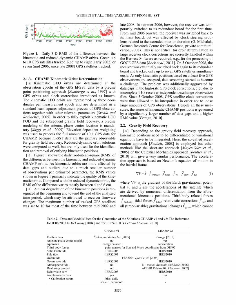
Figure 1. Daily 3-D RMS of the difference between thekinematic and reduced-dynamic CHAMP orbits. Green: upto 10 GPS satellites tracked. Red: up to eight (early 2002) orseven (mid 2006, since late 2008) GPS satellites tracked.

2.1.3. CHAMP Kinematic Orbit Determination[11] Kinematic LEO orbits are determined at the

observation epochs of the GPS hl-SST data by a precisepoint positioning approach [Zumberge et al., 1997] withGPS orbits and clock corrections introduced as known.The kinematic LEO orbits are represented by three coor-dinates per measurement epoch and are determined in astandard least squares adjustment process of GPS observa-tions together with other relevant parameters [Švehla andRothacher, 2005]. In order to fully exploit kinematic LEOPOD and the subsequent gravity field recovery, a precisemodeling of the antenna phase center location is manda-tory [Jäggi et al., 2009]. Elevation-dependent weightingwas used to process the full amount of 10 s GPS data forCHAMP, because hl-SST data are the primary observablefor gravity field recovery. Reduced-dynamic orbit solutionswere computed as well, but are only used for the identifica-tion and removal of outlying kinematic positions.

[12] Figure 1 shows the daily root-mean-square (RMS) ofthe differences between the kinematic and reduced-dynamicCHAMP orbits. As kinematic orbits are more affected bydata gaps and outliers due to a much smaller numberof observations per estimated parameter, the RMS valuesshown in Figure 1 primarily indicate the quality of the kine-matic orbits. Compared with the reduced-dynamic orbits, theRMS of the difference varies mostly between 4 and 6 cm.

[13] A clear degradation of the kinematic positions is rec-ognized at the beginning and toward the end of the analyzedtime period, which may be attributed to receiver firmwarechanges. The maximum number of tracked GPS satelliteswas set to 10 for most of the time between mid 2002 and

late 2008. In summer 2006, however, the receiver was tem-porarily switched to its redundant board for the first time.From mid 2006 onward, the receiver was switched back toits main board, but was affected by clock steering prob-lems related to the extended mission duration (G. Michalak,German Research Centre for Geoscience, private communi-cation, 2008). This is not critical for orbit determination aslarge receiver clock corrections are correctly handled withinthe Bernese Software as required, e.g., for the processing ofGOCE GPS data [Bock et al., 2011]. On 5 October 2008, thereceiver was eventually switched back again to its redundantboard and tracked only up to seven GPS satellites simultane-ously. As only kinematic positions based on at least five GPSobservations are accepted, data screening started to becomea challenge. The problem was additionally aggravated bydata gaps in the high-rate GPS clock corrections, e.g., due toincomplete 1 Hz receiver-independent exchange observationfiles. Since 5 October 2008, GPS satellite clock correctionswere thus allowed to be interpolated in order not to looselarge amounts of GPS observations. Despite all these mea-sures, the series of kinematic CHAMP positions is governedby a significantly larger number of data gaps and a higherRMS value [Prange, 2010].

2.2. Gravity Field Recovery[14] Depending on the gravity field recovery approach,

kinematic positions need to be differentiated or variationalequations have to be integrated. Here, the so-called accel-eration approach [Reubelt, 2008] is employed but othermethods like the short-arc approach [Mayer-Gürr et al.,2005] or the Celestial Mechanics approach [Beutler et al.,2010] will give a very similar performance. The accelera-tion approach is based on Newton’s equation of motion inthe inertial frame

rV = REx – Ef 3rdbody – Ef tides – Ef rel – Ef grav – Ef ng (1)

where rV is the gradient of the Earth gravitational poten-tial V, and REx are the accelerations of the satellite whichare derived by numerical differentiation from the afore-mentioned kinematic positions. Third-body related forcesEf 3rdbody, tidal forces Ef tides, relativistic corrections Ef rel, and

all (time-variable) gravitational changes Ef grav, which cannot

Table 2. Data and Models Used for the Generation of the Solutions CHAMP v1 and v2: The Referencefor IERS2003 Is McCarthy [2004] and for IERS2010 Is Petit and Luzum [2010]

CHAMP v1 CHAMP v2

Position data Švehla and Rothacher [2005] Prange [2010]Antenna phase center model no yesApproach energy balance accelerationThird-body forces point masses for Sun and Moon coordinates from DE405Solid Earth tide IERS2003 IERS2010Pole tide IERS2003 IERS2010Ocean tide FES2004; Lyard et al. [2006]Ocean pole tide IERS2003 IERS2010Atmospheric tide no N1-model; Biancale and Bode [2006]Dealiasing product no AOD1B Release 04; Flechtner [2007]Relativistic corr. IERS2003 IERS2010Accelerometer data yes no! Calibration param. bias: daily -

scale: 1 per month -

3850

WEIGELT ET AL.: TIME VARIABILITY FROM HL-SST

0 10 20 30 40 50 6010−12

10−11

10−10

10−9

10−8

10−7

degree l

unitl

ess

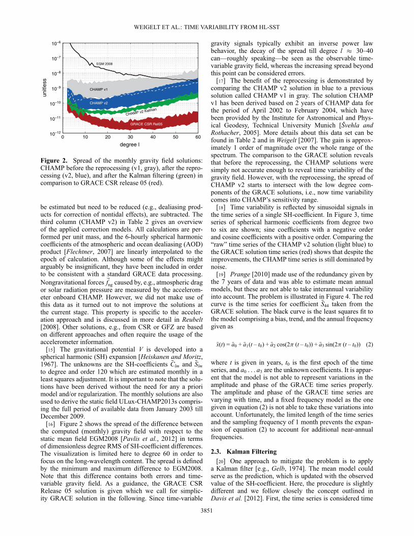
Figure 2. Spread of the monthly gravity field solutions:CHAMP before the reprocessing (v1, gray), after the repro-cessing (v2, blue), and after the Kalman filtering (green) incomparison to GRACE CSR release 05 (red).

be estimated but need to be reduced (e.g., dealiasing prod-ucts for correction of nontidal effects), are subtracted. Thethird column (CHAMP v2) in Table 2 gives an overviewof the applied correction models. All calculations are per-formed per unit mass, and the 6-hourly spherical harmoniccoefficients of the atmospheric and ocean dealiasing (AOD)product [Flechtner, 2007] are linearly interpolated to theepoch of calculation. Although some of the effects mightarguably be insignificant, they have been included in orderto be consistent with a standard GRACE data processing.Nongravitational forces Efng caused by, e.g., atmospheric dragor solar radiation pressure are measured by the accelerom-eter onboard CHAMP. However, we did not make use ofthis data as it turned out to not improve the solutions atthe current stage. This property is specific to the acceler-ation approach and is discussed in more detail in Reubelt[2008]. Other solutions, e.g., from CSR or GFZ are basedon different approaches and often require the usage of theaccelerometer information.

[15] The gravitational potential V is developed into aspherical harmonic (SH) expansion [Heiskanen and Moritz,1967]. The unknowns are the SH-coefficients NClm and NSlmto degree and order 120 which are estimated monthly in aleast squares adjustment. It is important to note that the solu-tions have been derived without the need for any a priorimodel and/or regularization. The monthly solutions are alsoused to derive the static field ULux-CHAMP2013s compris-ing the full period of available data from January 2003 tillDecember 2009.

[16] Figure 2 shows the spread of the difference betweenthe computed (monthly) gravity field with respect to thestatic mean field EGM2008 [Pavlis et al., 2012] in termsof dimensionless degree RMS of SH-coefficient differences.The visualization is limited here to degree 60 in order tofocus on the long-wavelength content. The spread is definedby the minimum and maximum difference to EGM2008.Note that this difference contains both errors and time-variable gravity field. As a guidance, the GRACE CSRRelease 05 solution is given which we call for simplic-ity GRACE solution in the following. Since time-variable

gravity signals typically exhibit an inverse power lawbehavior, the decay of the spread till degree l � 30–40can—roughly speaking—be seen as the observable time-variable gravity field, whereas the increasing spread beyondthis point can be considered errors.

[17] The benefit of the reprocessing is demonstrated bycomparing the CHAMP v2 solution in blue to a previoussolution called CHAMP v1 in gray. The solution CHAMPv1 has been derived based on 2 years of CHAMP data forthe period of April 2002 to February 2004, which havebeen provided by the Institute for Astronomical and Phys-ical Geodesy, Technical University Munich [Švehla andRothacher, 2005]. More details about this data set can befound in Table 2 and in Weigelt [2007]. The gain is approx-imately 1 order of magnitude over the whole range of thespectrum. The comparison to the GRACE solution revealsthat before the reprocessing, the CHAMP solutions weresimply not accurate enough to reveal time variability of thegravity field. However, with the reprocessing, the spread ofCHAMP v2 starts to intersect with the low degree com-ponents of the GRACE solutions, i.e., now time variabilitycomes into CHAMP’s sensitivity range.

[18] Time variability is reflected by sinusoidal signals inthe time series of a single SH-coefficient. In Figure 3, timeseries of spherical harmonic coefficients from degree twoto six are shown; sine coefficients with a negative orderand cosine coefficients with a positive order. Comparing the“raw” time series of the CHAMP v2 solution (light blue) tothe GRACE solution time series (red) shows that despite theimprovements, the CHAMP time series is still dominated bynoise.

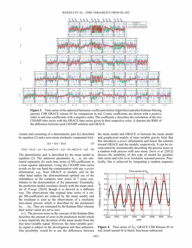
[19] Prange [2010] made use of the redundancy given bythe 7 years of data and was able to estimate mean annualmodels, but these are not able to take interannual variabilityinto account. The problem is illustrated in Figure 4. The redcurve is the time series for coefficient NS44 taken from theGRACE solution. The black curve is the least squares fit tothe model comprising a bias, trend, and the annual frequencygiven as

Nx(t) = Na0 + Na1(t – t0) + Na2 cos(2� (t – t0)) + Na3 sin(2� (t – t0)) (2)

where t is given in years, t0 is the first epoch of the timeseries, and a0 : : : a3 are the unknown coefficients. It is appar-ent that the model is not able to represent variations in theamplitude and phase of the GRACE time series properly.The amplitude and phase of the GRACE time series arevarying with time, and a fixed frequency model as the onegiven in equation (2) is not able to take these variations intoaccount. Unfortunately, the limited length of the time seriesand the sampling frequency of 1 month prevents the expan-sion of equation (2) to account for additional near-annualfrequencies.

2.3. Kalman Filtering[20] One approach to mitigate the problem is to apply

a Kalman filter [e.g., Gelb, 1974]. The mean model couldserve as the prediction, which is updated with the observedvalue of the SH-coefficient. Here, the procedure is slightlydifferent and we follow closely the concept outlined inDavis et al. [2012]. First, the time series is considered time

3851

WEIGELT ET AL.: TIME VARIABILITY FROM HL-SST

Figure 3. Time series of the spherical harmonic coefficients before (light blue) and after Kalman filtering(green); CSR GRACE release 05 for comparison in red. Cosine coefficients are shown with a positiveorder m and sine coefficients with a negative order. The coefficient � describes the correlation of the twoCHAMP time series with the GRACE time series given in their respective color. � denotes the RMS ofthe difference between each CHAMP solution and GRACE.

variant and consisting of a deterministic part Nx(t) describedby equation (2) and a zero-mean stochastic component •x(t).

x(t) = Nx(t) + •x(t) (3)

•x(t) = •a1(t – t0) + •a2 cos(2� (t – t0)) + •a3 sin(2� (t – t0)) (4)

The deterministic part is described by the mean model inequation (2). The unknown parameters Na0 : : : Na3 are esti-mated separately for each time series of SH-coefficients ina least squares adjustment. Using the CHAMP time seriesavoids on the one hand the contamination with any a prioriinformation, e.g., from GRACE or models, and on theother hand makes the aforementioned optimal use of theredundancy as the complete time series of 7 years con-tributes to the determination of the parameter. Essentially,the prediction model correlates closely with the mean mod-els of Prange [2010] though it is derived in a differentway. The observations (the original time series of a sin-gle SH-coefficient) are reduced by the mean model, andthe residuum is seen as the observations of a stochasticzero-mean process which is described by the parameters•a1 : : : •a3. They are estimated by the Kalman filter whereastheir initial values are set to zero.

[21] The process noise in the concept of the Kalman filterdescribes the amount of error in the prediction model whichis here implicitly the deviation of the mean model from thetrue time-variable signal. However, the time-variable grav-ity signal is subject to the investigation and thus unknown.One possibility would be to use the differences between

the mean model and GRACE or between the mean modeland geophysical models of time-variable gravity field. Butthis introduces a priori information and biases the solutiontoward GRACE and the models, respectively. It can be cir-cumvented by stochastically describing the process noise asa random walk process with zero mean. Davis et al. [2012]discuss the suitability of this type of model for geodetictime series and refer to as stochastic seasonal process. Prac-tically, this is achieved by integrating a random sequence

2003 2004 2005 2006 2007 2008 2009 2010−0.8

−0.6

−0.4

−0.2

0

0.2

0.4

0.6

0.8

year

Figure 4. Time series of NS44: GRACE CSR Release 05 inred; trend+annual fit in black; bias/mean subtracted.

3852

WEIGELT ET AL.: TIME VARIABILITY FROM HL-SST

2003 2004 2005 2006 2007 2008 2009 2010−1

−0.8

−0.6

−0.4

−0.2

0

0.2

0.4

0.6

0.8

1

year

Time series of S44

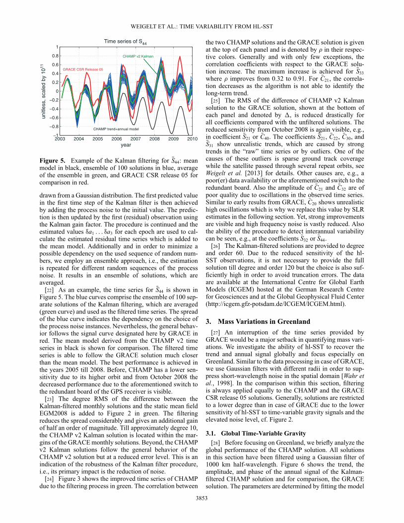
Figure 5. Example of the Kalman filtering for NS44: meanmodel in black, ensemble of 100 solutions in blue, averageof the ensemble in green, and GRACE CSR release 05 forcomparison in red.

drawn from a Gaussian distribution. The first predicted valuein the first time step of the Kalman filter is then achievedby adding the process noise to the initial value. The predic-tion is then updated by the first (residual) observation usingthe Kalman gain factor. The procedure is continued and theestimated values •a1 : : : •a3 for each epoch are used to cal-culate the estimated residual time series which is added tothe mean model. Additionally and in order to minimize apossible dependency on the used sequence of random num-bers, we employ an ensemble approach, i.e., the estimationis repeated for different random sequences of the processnoise. It results in an ensemble of solutions, which areaveraged.

[22] As an example, the time series for NS44 is shown inFigure 5. The blue curves comprise the ensemble of 100 sep-arate solutions of the Kalman filtering, which are averaged(green curve) and used as the filtered time series. The spreadof the blue curve indicates the dependency on the choice ofthe process noise instances. Nevertheless, the general behav-ior follows the signal curve designated here by GRACE inred. The mean model derived from the CHAMP v2 timeseries in black is shown for comparison. The filtered timeseries is able to follow the GRACE solution much closerthan the mean model. The best performance is achieved inthe years 2005 till 2008. Before, CHAMP has a lower sen-sitivity due to its higher orbit and from October 2008 thedecreased performance due to the aforementioned switch tothe redundant board of the GPS receiver is visible.

[23] The degree RMS of the difference between theKalman-filtered monthly solutions and the static mean fieldEGM2008 is added to Figure 2 in green. The filteringreduces the spread considerably and gives an additional gainof half an order of magnitude. Till approximately degree 10,the CHAMP v2 Kalman solution is located within the mar-gins of the GRACE monthly solutions. Beyond, the CHAMPv2 Kalman solutions follow the general behavior of theCHAMP v2 solution but at a reduced error level. This is anindication of the robustness of the Kalman filter procedure,i.e., its primary impact is the reduction of noise.

[24] Figure 3 shows the improved time series of CHAMPdue to the filtering process in green. The correlation between

the two CHAMP solutions and the GRACE solution is givenat the top of each panel and is denoted by � in their respec-tive colors. Generally and with only few exceptions, thecorrelation coefficients with respect to the GRACE solu-tion increase. The maximum increase is achieved for NS33where � improves from 0.32 to 0.91. For NC21, the correla-tion decreases as the algorithm is not able to identify thelong-term trend.

[25] The RMS of the difference of CHAMP v2 Kalmansolution to the GRACE solution, shown at the bottom ofeach panel and denoted by �, is reduced drastically forall coefficients compared with the unfiltered solutions. Thereduced sensitivity from October 2008 is again visible, e.g.,in coefficient NS21 or NC40. The coefficients NS21, NC22, NC30, andNS31 show unrealistic trends, which are caused by strongtrends in the “raw” time series or by outliers. One of thecauses of these outliers is sparse ground track coveragewhile the satellite passed through several repeat orbits, seeWeigelt et al. [2013] for details. Other causes are, e.g., apoor(er) data availability or the aforementioned switch to theredundant board. Also the amplitude of NC21 and NC32 are ofpoor quality due to oscillations in the observed time series.Similar to early results from GRACE, NC20 shows unrealistichigh oscillations which is why we replace this value by SLRestimates in the following section. Yet, strong improvementsare visible and high frequency noise is vastly reduced. Alsothe ability of the procedure to detect interannual variabilitycan be seen, e.g., at the coefficients NS32 or NS44.

[26] The Kalman-filtered solutions are provided to degreeand order 60. Due to the reduced sensitivity of the hl-SST observations, it is not necessary to provide the fullsolution till degree and order 120 but the choice is also suf-ficiently high in order to avoid truncation errors. The dataare available at the International Centre for Global EarthModels (ICGEM) hosted at the German Research Centrefor Geosciences and at the Global Geophysical Fluid Center(http://icgem.gfz-potsdam.de/ICGEM/ICGEM.html).

3. Mass Variations in Greenland[27] An interruption of the time series provided by

GRACE would be a major setback in quantifying mass vari-ations. We investigate the ability of hl-SST to recover thetrend and annual signal globally and focus especially onGreenland. Similar to the data processing in case of GRACE,we use Gaussian filters with different radii in order to sup-press short-wavelength noise in the spatial domain [Wahr etal., 1998]. In the comparison within this section, filteringis always applied equally to the CHAMP and the GRACECSR release 05 solutions. Generally, solutions are restrictedto a lower degree than in case of GRACE due to the lowersensitivity of hl-SST to time-variable gravity signals and theelevated noise level, cf. Figure 2.

3.1. Global Time-Variable Gravity[28] Before focusing on Greenland, we briefly analyze the

global performance of the CHAMP solution. All solutionsin this section have been filtered using a Gaussian filter of1000 km half-wavelength. Figure 6 shows the trend, theamplitude, and phase of the annual signal of the Kalman-filtered CHAMP solution and for comparison, the GRACEsolution. The parameters are determined by fitting the model

3853

WEIGELT ET AL.: TIME VARIABILITY FROM HL-SST

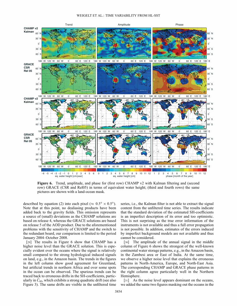
Figure 6. Trend, amplitude, and phase for (first row) CHAMP v2 with Kalman filtering and (secondrow) GRACE (CSR and Rel05) in terms of equivalent water height; (third and fourth rows) the samepictures are shown with a land-ocean mask.

described by equation (2) into each pixel (� 0.5ı � 0.5ı).Note that at this point, no dealiasing products have beenadded back to the gravity fields. This omission representsa source of (small) deviations as the CHAMP solutions arebased on release 4, whereas the GRACE solutions are basedon release 5 of the AOD product. Due to the aforementionedproblems with the sensitivity of CHAMP and the switch tothe redundant board, our comparison is limited to the periodJanuary 2004–October 2008.

[29] The results in Figure 6 show that CHAMP has ahigher noise level than the GRACE solution. This is espe-cially evident over the oceans where the signal is relativelysmall compared to the strong hydrological induced signalson land, e.g., in the Amazon basin. The trends in the figuresin the left column show good agreement for Greenland,but artificial trends in northern Africa and over some spotsin the ocean can be observed. The spurious trends can betraced back to erroneous drifts in the SH-coefficients, partic-ularly in NC60, which exhibits a strong quadratic drift (see alsoFigure 3). The same drifts are visible in the unfiltered time

series, i.e., the Kalman filter is not able to extract the signalcontent from the unfiltered time series. The results indicatethat the standard deviation of the estimated SH-coefficientsis an imperfect description of its error and too optimistic.This is not surprising as the true error information of theinstruments is not available and thus a full error propagationis not possible. In addition, estimates of the errors inducedby imperfect background models are not available and thuscannot be considered.

[30] The amplitude of the annual signal in the middlecolumn of Figure 6 shows the strongest of the well-knowncontinental water storage patterns, e.g., in the Amazon basin,in the Zambesi area or East of India. At the same time,we observe a higher noise level that explains the erroneouspatterns in North-America, Europe, and North-East Asia.The corresponding CHAMP and GRACE phase patterns inthe right column agree particularly well in the NorthernHemisphere.

[31] As the noise level appears dominant on the oceans,we added the same two figures masking out the oceans in the

3854

WEIGELT ET AL.: TIME VARIABILITY FROM HL-SST

KELY

THU2

QAQ1

KULU

(a) (b) (c)

(d) (e) (f)

(g) (h) (i)

(j) (k) (i)

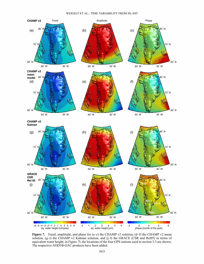
Figure 7. Trend, amplitude, and phase for (a–c) the CHAMP v2 solution, (d–f) the CHAMP v2 meansolution, (g–i) the CHAMP v2 Kalman solution, and (j–l) the GRACE (CSR and Rel05) in terms ofequivalent water height; in Figure 7l, the locations of the four GPS stations used in section 3.3 are shown.The respective AOD1B-GAC products have been added.

3855

WEIGELT ET AL.: TIME VARIABILITY FROM HL-SST

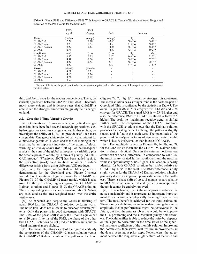
Table 3. Signal RMS and Difference RMS With Respect to GRACE in Terms of Equivalent Water Height andLocation of the Peak Value for the Solutionsa

RMS RMSsignal �GRACE Peak Location

Trend: (cm/yr) (cm/yr) (cm/yr) �P �PCHAMP v2 2.79 2.78 –3.60 50.4ıW 66.0ıNCHAMP mean 3.70 1.54 –4.60 41.2ıW 66.0ıNCHAMP Kalman 2.99 0.63 –4.36 46.1ıW 66.0ıNGRACE 2.78 - –4.39 42.1ıW 69.2ıNAmplitude: (cm) (cm) (cm) �P �PCHAMP v2 6.53 1.75 8.87 44.6ıW 71.2ıNCHAMP mean 4.84 0.66 6.75 56.2ıW 69.7ıNCHAMP Kalman 4.97 0.54 6.81 56.1ıW 70.1ıNGRACE 4.92 - 6.33 47.4ıW 71.8ıNPhase: (Month) (Month) - - -CHAMP v2 4.27 0.71 - - -CHAMP mean 4.16 0.76 - - -CHAMP Kalman 4.24 0.72 - - -GRACE 4.62 - - - -

aIn case of the trend, the peak is defined as the maximum negative value, whereas in case of the amplitude, it is the maximumpositive value.

third and fourth rows for the readers convenience. There, the(visual) agreement between CHAMP and GRACE becomesmuch more evident and it demonstrates that CHAMP isable to see the strongest time-variable gravity field changeson land.

3.2. Greenland Time-Variable Gravity[32] Observations of time-variable gravity field changes

over land have benefited several research applications, e.g.,hydrological or ice-mass change studies. In this section, weinvestigate the ability of hl-SST to provide useful ice-masschange data. One geographic region of particular interest forclimate change studies is Greenland as the ice melting in thatarea may be an important indicator of the extent of globalwarming, cf. Velicogna and Wahr [2006]. For the subsequentanalysis, the sum of the global atmospheric variability plusthe oceanic pressure variability in terms of gravity (AOD1B-GAC product) [Flechtner, 2007] has been added back tothe respective gravity field solutions in order to reducedifferences arising from using different AOD products.

[33] First, the impact of the Kalman filter process isdemonstrated for the Greenland area. Figure 7 showsfour different solutions: Figures 7a–7c, the CHAMP v2;Figures 7d–7f, the CHAMP v2 mean model, which is alsoused for the prediction; Figures 7g–7i, the CHAMP v2Kalman solution; and Figures 7j–7l, the GRACE solution.The corresponding statistics are shown in Table 3. Valuesare calculated as the area-weighted mean over the entirevisible area.

[34] As expected and despite the Gaussian filtering ofagain 1000 km, the CHAMP v2 solution performs worst.The noise level does not allow us to observed realistic pat-terns. Only the phase is in good agreement with GRACE.The RMS of the phase shift is only 0.71 month equivalentto � 20 days. In terms of the RMS, the phase of the othertwo CHAMP solutions do not produce better results but thevisual pattern changes slightly.

[35] The most interesting aspect of the figure is certainlythe comparison of the CHAMP v2 mean solution versusthe CHAMP v2 Kalman solution. The pattern of the trend

(Figures 7a, 7d, 7g, 7j) shows the strongest disagreement.The mean solution has a stronger trend in the northern part ofGreenland. This is confirmed by the statistics in Table 3. Theoverall signal RMS is 2.99 cm/year for CHAMP and 2.78cm/year for GRACE. The signal RMS is� 23 % higher andalso the difference RMS to GRACE is almost a factor 2.5higher. The peak, i.e., maximum negative trend, is shiftedfurther north. The comparison of the CHAMP solutionswith the GRACE solutions shows that the Kalman solutionproduces the best agreement although the pattern is slightlyrotated and shifted to the south-west. The magnitude of thepeak is –4.36 cm/year in terms of equivalent water height,which is just� 0.6% smaller than in case of GRACE.

[36] The amplitude pattern in Figures 7b, 7e, 7h, and 7kfor the CHAMP v2 mean and the CHAMP v2 Kalman solu-tion is almost identical. Only in the extreme north-easterncorner can we see a difference. In comparison to GRACE,the maxima are located further south-west and the maximavalue is approximately � 8 % higher. The location is nearlyidentical for both CHAMP solutions but shifted relative toGRACE by � 9ı to the west. The RMS difference is onlyslightly better for the CHAMP v2 Kalman solution, which isprimarily due to an improved phase estimation in the north-east. There, a phase shift of up to 2 months occurs relativeto GRACE, which can be reduced by the Kalman approachthough it cannot be entirely removed.

[37] In conclusion, the Kalman approach reduces thenoise considerably and it represents an important improve-ment for extracting a geophysically meaningful spatial pat-tern. The most benefit is achieved for the trend estimation.There is only a slight improvement in determining the annualamplitude. Better performance might be achievable in thefuture, but then the primary objective would be to improvethe GPS positioning and the subsequent gravity field recov-ery. The Kalman filter is able to reduce the noise but dependson the signal to noise ratio in the time series of the spheri-cal harmonic coefficients of the monthly solution. Improvingthe coefficients themselves will require improvements inthe data processing at prior steps. Nevertheless, the agree-ment between the long-wavelength features of the trend and

3856

WEIGELT ET AL.: TIME VARIABILITY FROM HL-SST

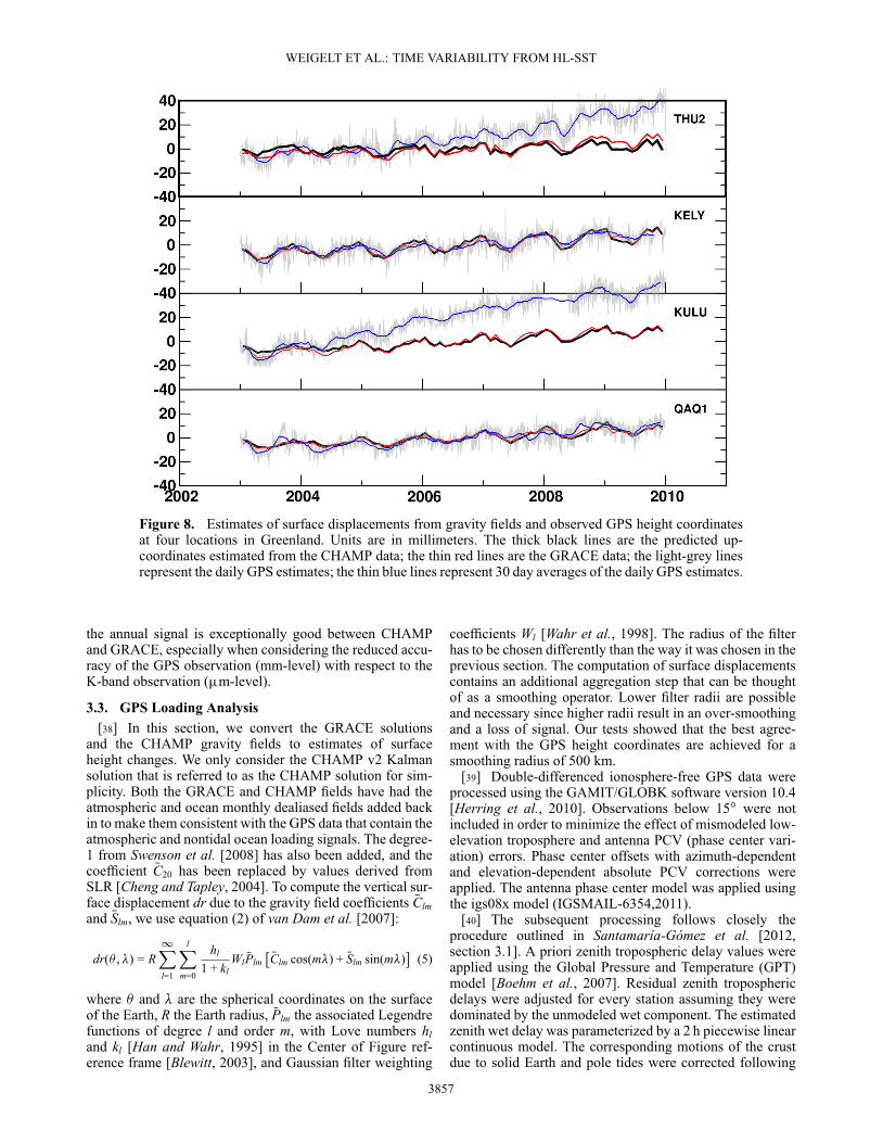
Figure 8. Estimates of surface displacements from gravity fields and observed GPS height coordinatesat four locations in Greenland. Units are in millimeters. The thick black lines are the predicted up-coordinates estimated from the CHAMP data; the thin red lines are the GRACE data; the light-grey linesrepresent the daily GPS estimates; the thin blue lines represent 30 day averages of the daily GPS estimates.

the annual signal is exceptionally good between CHAMPand GRACE, especially when considering the reduced accu-racy of the GPS observation (mm-level) with respect to theK-band observation (�m-level).

3.3. GPS Loading Analysis[38] In this section, we convert the GRACE solutions

and the CHAMP gravity fields to estimates of surfaceheight changes. We only consider the CHAMP v2 Kalmansolution that is referred to as the CHAMP solution for sim-plicity. Both the GRACE and CHAMP fields have had theatmospheric and ocean monthly dealiased fields added backin to make them consistent with the GPS data that contain theatmospheric and nontidal ocean loading signals. The degree-1 from Swenson et al. [2008] has also been added, and thecoefficient NC20 has been replaced by values derived fromSLR [Cheng and Tapley, 2004]. To compute the vertical sur-face displacement dr due to the gravity field coefficients NClmand NSlm, we use equation (2) of van Dam et al. [2007]:

dr(� ,�) = R1X

l=1

lX

m=0

hl

1 + klWl NPlm

�NClm cos(m�) + NSlm sin(m�)

�(5)

where � and � are the spherical coordinates on the surfaceof the Earth, R the Earth radius, NPlm the associated Legendrefunctions of degree l and order m, with Love numbers hland kl [Han and Wahr, 1995] in the Center of Figure ref-erence frame [Blewitt, 2003], and Gaussian filter weighting

coefficients Wl [Wahr et al., 1998]. The radius of the filterhas to be chosen differently than the way it was chosen in theprevious section. The computation of surface displacementscontains an additional aggregation step that can be thoughtof as a smoothing operator. Lower filter radii are possibleand necessary since higher radii result in an over-smoothingand a loss of signal. Our tests showed that the best agree-ment with the GPS height coordinates are achieved for asmoothing radius of 500 km.

[39] Double-differenced ionosphere-free GPS data wereprocessed using the GAMIT/GLOBK software version 10.4[Herring et al., 2010]. Observations below 15ı were notincluded in order to minimize the effect of mismodeled low-elevation troposphere and antenna PCV (phase center vari-ation) errors. Phase center offsets with azimuth-dependentand elevation-dependent absolute PCV corrections wereapplied. The antenna phase center model was applied usingthe igs08x model (IGSMAIL-6354,2011).

[40] The subsequent processing follows closely theprocedure outlined in Santamaría-Gómez et al. [2012,section 3.1]. A priori zenith tropospheric delay values wereapplied using the Global Pressure and Temperature (GPT)model [Boehm et al., 2007]. Residual zenith troposphericdelays were adjusted for every station assuming they weredominated by the unmodeled wet component. The estimatedzenith wet delay was parameterized by a 2 h piecewise linearcontinuous model. The corresponding motions of the crustdue to solid Earth and pole tides were corrected following

3857

WEIGELT ET AL.: TIME VARIABILITY FROM HL-SST

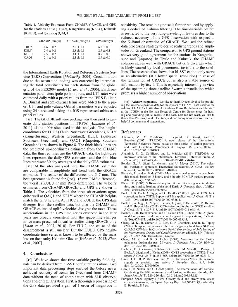
Table 4. Velocity Estimates From CHAMP, GRACE, and GPSfor the Stations Thule (THU2), Kangerlussuaq (KELY), Kulusuk(KULU), and Qaqortoq (QAQ1)

CHAMP (mm/yr) GRACE (mm/yr ) GPS (mm/yr)

THU2 0.6˙ 0.2 2.0˙ 0.1 6.2˙ 0.0KELY 2.4˙ 0.2 2.8˙ 0.1 2.7˙ 0.1KULU 2.5˙ 0.2 3.1˙ 0.1 8.7˙ 0.0QAQ1 2.1˙ 0.2 2.1˙ 0.1 2.9˙ 0.0

the International Earth Rotation and Reference Systems Ser-vice (IERS) Conventions [McCarthy, 2004]. Crustal motiondue to the ocean tide loading was corrected by interpolat-ing the tidal constituents for each station from the globalgrid of the FES2004 model [Lyard et al., 2006]. Earth ori-entation parameters (pole position, rate, and UT1 rate) wereestimated daily with a priori values from the IERS BulletinA. Diurnal and semi-diurnal terms were added to the a pri-ori UT1 and pole values. Orbital parameters were adjustedusing 24 h arcs and taking the IGS reprocessed orbits as apriori values.

[41] The GLOBK software package was then used to gen-erate daily station positions in ITRF08 [Altamimi et al.,2011] of the 400+ sites used in this analysis. The height-coordinates for THU2 (Thule, Northwest Greenland), KELY(Kangerlussuaq, Western Greenland), KULU (Kulusuk,Southeast Greenland), and QAQ1 (Qaqortoq, SouthernGreenland) are shown in Figure 8. The thick black lines arethe predicted up-coordinates estimated from the CHAMPdata; the thin red lines are the GRACE data; the light-greylines represent the daily GPS estimates; and the thin bluelines represent 30 day averages of the daily GPS estimates.

[42] At the sites analyzed here, the CHAMP estimatesare comparable in amplitude and trend with the GRACEestimates. The scatter of the differences are 5–7 mm. Thebest agreement is found for QAQ1 (5 mm RMS difference);the worst is KULU (7 mm RMS difference). The velocityestimates from CHAMP, GRACE, and GPS are shown inTable 4. The velocities from the three observations agreequite well at QAQ1 and KELY where the CHAMP heightsmatch the GPS heights. At THU2 and KULU, the GPS datadiverges from the satellite data, but also the CHAMP andGRACE estimated uplift velocities disagree the most. Theseaccelerations in the GPS time series observed in the lateryears are broadly consistent with the space-time changesin ice mass presented in earlier studies using GRACE only[Khan et al., 2007, 2010]. For THU2, the cause of thedisagreement is still unclear. But the KULU GPS height-coordinate time series is known to be affected by the massloss on the nearby Helheim Glacier [Wahr et al., 2013; Khanet al., 2007].

4. Conclusions[43] We have shown that time-variable gravity field sig-

nals can be derived from hl-SST configurations alone. Twoimportant data processing steps enabled the before neverachieved recovery of trends for Greenland from CHAMPdata without the need of combination with SLR observa-tions and/or regularization. First, a thorough reprocessing ofthe GPS data provided a gain of 1 order of magnitude in

sensitivity. The remaining noise is further reduced by apply-ing a dedicated Kalman filtering. The time-variable patternis restricted to the very long-wavelength features due to thereduced accuracy of the GPS observation with respect tothe K-Band observation of GRACE. We used the refineddata processing strategy to derive realistic trends and ampli-tudes for Greenland. The comparison to GPS ground stationsshows very good agreement for the stations in Kangerlus-suaq and Qaqortoq. In Thule and Kulusuk, the CHAMPsolution agrees well with GRACE but GPS diverges whichis likely caused by local phenomena invisible to the satel-lites. The research also shows that hl-SST cannot only serveas an alternative (at a lower spatial resolution) in case ofthe termination of GRACE but is also a viable source ofinformation by itself. This is especially interesting in viewof the upcoming three satellite Swarm constellation whichpromises a higher number of observations.

[44] Acknowledgments. We like to thank Drazen Švehla for provid-ing the kinematic position data for the 2 years of CHAMP data used for thesolution CHAMP v1. We also like to thank Franz Barthelmes and the staffat the ICGEM at the German Research Centre for Geosciences for host-ing and providing public access to the data. Last but not least, we like tothank Tom Parsons, Frank Flechtner, and one anonymous reviewer for theirhelpful comments and suggestions.

ReferencesAltamimi, Z., X. Collilieux, J. Legrand, B. Garayt, and C.

Boucher (2007), ITRF2005: A new release of the InternationalTerrestrial Reference Frame based on time series of station positionsand Earth Orientation Parameters, J. Geophys. Res., 112, B09401,doi:10.1029/2007JB004949.

Altamimi, Z., X. Collilieux, and L. Métivier (2011), ITRF2008: Animproved solution of the International Terrestrial Reference Frame, J.Geod., 85(8), 457–473, doi:10.1007/s00190-011-0444-4.

Beutler, G., A. Jäggi, L. Mervart, and U. Meyer (2010), The celes-tial mechanics approach: Theoretical foundations, J. Geod., 84(10),605–624, doi:10.1007/s00190-010-0401-7.

Biancale, R., and A. Bode (2006), Mean annual and seasonal atmospherictide models based on 3-hourly and 6-hourly ECMWF surface pressuredata, Tech. Rep. STR 06/01.

Blewitt, G. (2003), Self-consistency in reference frames, geocenter defini-tion, and surface loading of the solid Earth, J. Geophys. Res., 108(B2),2103, doi:10.1029/2002JB002082.

Bock, H., R. Dach, A. Jäggi, and G. Beutler (2009), High-rate GPS clockcorrections from CODE: Support of 1 Hz applications, J. Geod., 83(11),1083–1094, doi:10.1007/s00190-009-0326-1.

Bock, H., A. Jäggi, U. Meyer, P. Visser, J. Ijssel, T. Helleputte, M. Heinze,and U. Hugentobler (2011), GPS-derived orbits for the GOCE satellite,J. Geod., 85(11), 807–818, doi:10.1007/s00190-011-0484-9.

Boehm, J., R. Heinkelmann, and H. Schuh (2007), Short Note: A globalmodel of pressure and temperature for geodetic applications, J. Geod.,81(10), 679–683, doi:10.1007/s00190-007-0135-3.

Cheng, M. K., B. Gunter, J. C. Ries, D. P. Chambers, and B. D. Tapley(2002), Temporal variations in the Earth’s gravity field from SLR andCHAMP GPS data, in Gravity and Geoid: Proceedings of 3rd Meeting ofthe International Gravity and Geoid Commission, edited by I. N. Tziavos,pp. 237–242, Ziti, Thessaloniki, Greece.

Cheng, M. K., and B. D. Tapley (2004), Variations in the Earth’soblateness during the past 28 years, J. Geophys. Res., 109, B09402,doi:10.1029/2004JB003028.

Dach, R., E. Brockmann, S. Schaer, G. Beutler, M. Meindl, L. Prange, H.Bock, A. Jäggi, and L. Ostini (2009), GNSS processing at CODE: Statusreport, J. Geod., 83(3-4), 353–365, doi:10.1007/s00190-008-0281-2.

Davis, J. L., B. P. Wernicke, and M. E. Tamisiea (2012), On seasonalsignals in geodetic time series, J. Geophys. Res., 117, 1–10,doi:10.1029/2011JB008690.

Dow, J., R. Neilan, and G. Gendt (2005), The International GPS Service:Celebrating the 10th anniversary and looking to the next decade, Adv.Space Res., 36(3), 320–326, doi:10.1016/j.asr.2005.05.125.

European Space Agency (1999), Gravity field and steady-state oceancirculation mission, Eur. Space Agency Rep. ESA SP-1233(1), edited byB. Battrick, 217 pp.

3858

WEIGELT ET AL.: TIME VARIABILITY FROM HL-SST

European Space Agency (2004), The Earth’s magnetic field and environ-ment explorers, Eur. Space Agency Rep. ESA SP-1279(6), edited byB. Battrick, 70 pp.

Flechtner, F. (2007), AOD1B Product Description Document for ProductReleases 01 to 04, Rev. 3.1, April 13, 2007, GRACE project document,327–750.

Flechtner, F., P. Morton, M. Watkins, and F. Webb (2013), Status of theGRACE follow-on mission, Proceedings of the International Associationof Geodesy Symposia Gravity, Geoid and Height System (GGHS2012),9.-11.10.2012, Venice, Italy, IAGS-D-12-00141, (accepted).

Gelb, A. (1974), Applied Optimal Estimation, 374 pp., MIT Press,Cambridge, Mass.

Han, D., and J. Wahr (1995), The viscoelastic relaxation of a realisticallystratified Earth, and a further analysis of postglacial rebound, Geophys.J. Int., 120(2), 287–311, doi:10.1111/j.1365-246X.1995.tb01819.x.

Heiskanen, W., and H. Moritz (1967), Physical Geodesy, 364 pp., W. H.Freeman, San Francisco, Calif.

Herring, T. A., R. W. King, and S. C. McClusky (2010), GAMIT: ReferenceManual Version 10.34, Tech. Rep., Mass. Inst. of Technol., Cambridge.

Hugentobler, U. (2004), CODE high rate clocks, IGS Mail No. 4913, IGSCentral Bureau Information System.

Jäggi, A., R. Dach, O. Montenbruck, U. Hugentobler, H. Bock, and G.Beutler (2009), Phase center modeling for LEO GPS receiver anten-nas and its impact on precise orbit determination, J. Geod., 83(12),1145–1162, doi:10.1007/s00190-009-0333-2.

Khan, S. A., J. Wahr, L. A. Stearns, G. S. Hamilton, T. van Dam,K. M. Larson, and O. Francis (2007), Elastic uplift in southeastGreenland due to rapid ice mass loss, Geophys. Res. Lett., 34, L21701,doi:10.1029/2007GL031468.

Khan, S. A., J. Wahr, M. Bevis, I. Velicogna, and E. Kendrick (2010),Spread of ice mass loss into northwest Greenland observed by GRACEand GPS, Geophys. Res. Lett., 37, L06501, doi:10.1029/2010GL042460.

Lin, T., C. Hwang, T.-P. Tseng, and B. Chao (2012), Low-degree gravitychange from GPS data of COSMIC and GRACE satellite missions, J.Geodyn., 53, 34–42, doi:10.1016/j.jog.2011.08.004.

Lyard, F., F. Lefevre, T. Letellier, and O. Francis (2006), Modelling theglobal ocean tides: Modern insights from FES2004, Ocean Dyn., 56(5-6),394–415, doi:10.1007/s10236-006-0086-x.

Mayer-Gürr, T., K. Ilk, A. Eicker, and M. Feuchtinger (2005), ITG-CHAMP01: A CHAMP gravity field model from short kinematicarcs over a one-year observation period, J. Geod., 78(7-8), 462–480,doi:10.1007/s00190-004-0413-2.

McCarthy, D. D. (2004), IERS Conventions (2003), Tech. Rep. No. 32,Verlag des Bundesamts für Kartographie und Geodäsie.

Pavlis, N. K., S. A. Holmes, S. C. Kenyon, and J. K. Factor(2012), The development and evaluation of the Earth GravitationalModel 2008 (EGM2008), J. Geophys. Res., 117, B04406, doi:10.1029/2011JB008916.

Petit, G., and B. Luzum (2010), IERS conventions (2010), Tech. Rep. 36,Verlag des Bundesamts für Kartographie und Geodäsie.

Prange, L. (2010), Global gravity field determination using the GPS mea-surements made onboard the low Earth orbiting satellite CHAMP, PhDthesis, Geodätisch-geophysikalische Arbeiten in der Schweiz, vol. 81,http://www.sgc.ethz.ch/sgc-volumes/sgk-81.pdf.

Qiang, Z., and P. Moore (2005), On the contribution of CHAMP to tem-poral gravity field variation studies, in Earth Observation With CHAMP,Results From Three Years in Orbit, edited by C. Reigber et al., pp. 19–24,Springer, Berlin.

Reigber, C., H. Lühr, and P. Schwintzer (2001), Announcement of opportu-nity for CHAMP, Tech. Rep. CH-GFZ-AO-001.

Reubelt, T. (2008), Harmonische Gravitationsfeldanalyse aus GPS- ver-messenen kinematischen Bahnen niedrig fliegender Satelliten vom TypCHAMP, GRACE und GOCE mit einem hoch auflösenden Beschleuni-gungsansatz, PhD thesis, Universität Stuttgart.

Santamaría-Gómez, A., M. Gravelle, X. Collilieux, M. Guichard, B. M.Míguez, P. Tiphaneau, and G. Wöppelmann (2012), Mitigating theeffects of vertical land motion in tide gauge records using a state-of-the-art GPS velocity field, Global Planet. Change, 98-99, 6–17,doi:10.1016/j.gloplacha.2012.07.007.

Schaer, S., and R. Dach (2008), Model changes made at CODE, IGS MailNo. 5771, IGS Central Bureau Information System.

Schmid, R., P. Steigenberger, G. Gendt, M. Ge, and M. Rothacher (2007),Generation of a consistent absolute phase-center correction modelfor GPS receiver and satellite antennas, J. Geod., 81(12), 781–798,doi:10.1007/s00190-007-0148-y.

Sneeuw, N., C. Gerlach, D. Svehla, and C. Gruber (2002), A first attemptat time-variable gravity recovery from CHAMP using the energy balanceapproach, in Gravity and Geoid: Proceedings of 3rd Meeting of the Inter-national Gravity and Geoid Commission, edited by I. N. Tziavos, pp.237–242, Ziti, Thessaloniki, Greece.

Steigenberger, P., M. Rothacher, R. Dietrich, M. Fritsche, A. Rülke, and S.Vey (2006), Reprocessing of a global GPS network, J. Geophys. Res.,111, B05402, doi:10.1029/2005JB003747.

Švehla, D., and M. Rothacher (2005), Kinematic precise orbit determinationfor gravity field determination, in A Window on the Future of Geodesy,Int. Assoc. of Geod. Symp., vol. 128, pp. 181–188, Springer, Berlin,doi:10.1007/3-540-27432-4_32.

Swenson, S., D. Chambers, and J. Wahr (2008), Estimating geocentervariations from a combination of GRACE and ocean model output, J.Geophys. Res., 113, B08410, doi:10.1029/2007JB005338.

Tapley, B. D., et al. (1996), The Joint Gravity Model 3, J. Geophys. Res.,101(B12), 28,029–28,049, doi:10.1029/96JB01645.

Tapley, B. D., S. Bettadpur, J. C. Ries, P. F. Thompson, and M. M. Watkins(2004), GRACE measurements of mass variability in the Earth system,Science, 305(5683), 503–5, doi:10.1126/science.1099192.

van Dam, T., J. Wahr, and D. Lavallée (2007), A comparison of annualvertical crustal displacements from GPS and Gravity Recovery and Cli-mate Experiment (GRACE) over Europe, J. Geophys. Res., 112, B03404,doi:10.1029/2006JB004335.

Velicogna, I., and J. Wahr (2006), Acceleration of Greenland ice mass lossin spring 2004, Nature, 443(7109), 329–31, doi:10.1038/nature05168.

Wahr, J., M. Molenaar, and F. Bryan (1998), Time variability of theEarth’s gravity field: Hydrological and oceanic effects and their possibledetection using GRACE, J. Geophys. Res., 103(B12), 30,205–30,229,doi:10.1029/98JB02844.

Wahr, J., T. Kahn, T. van Dam, L. Liu, J. H. van Angelen, M. R. vanden Broeke, and C. M. Meertens (2013), The use of GPS horizontalsfor loading studies, with applications to northern California and southeastGreenland, J. Geophys. Res. Solid Earth, 118, 1795–1806, doi:10.1002/jgrb.50104.

Weigelt, M. L. (2007), Global and local gravity field recovery from satellite-to-satellite tracking, PhD thesis, Univ. of Calgary.

Weigelt, M., N. Sneeuw, E. J. O. Schrama, and P. N. A. M. Visser(2013), An improved sampling rule for mapping geopotential func-tions of a planet from a near polar orbit, J. Geod., 87(2), 127–142,doi:10.1007/s00190-012-0585-0.

Zumberge, J. F., M. B. Heflin, D. C. Jefferson, M. M. Watkins, andF. H. Webb (1997), Precise point positioning for the efficient and robustanalysis of GPS data from large networks, J. Geophys. Res., 102(B3),5005–5017, doi:10.1029/96JB03860.

3859