Times Series Analysis Evaluating Mortality Rates and the Differences of How States

Investigate Deaths

by

Jordan M. Bruhn

A thesis submitted in partial fulfillment of the

requirements for the degree of

Master of Science

in

Criminology and Criminal Justice

Thesis Committee:

Mark Harmon Leymon, Chair

Kathryn Wuschke

Danielle McGurrin

Portland State University

2020

i

Abstract

Mortality statistics are essential to both public health and criminal justice systems.

The causes of death that are determined by death investigators influence whether a

criminal investigation is opened or not. Prior research suggests a high degree of

variability for death investigator requirements across states, which may attribute to

inaccurate death reporting. This research provides a 20-year evaluation of the differences

in state death investigation laws and their impacts on rates of mortality. This study

examines the variation in mortality rates by answering if there is a difference in mortality

rates for states requiring medical examiners and states requiring coroners due to the broad

range of job qualifications. Specifically, this study evaluates rates of homicide and

suicide. The research question was evaluated using a Prais-Winsten regression model

with panel-corrected standard errors to analyze if certain death investigators are

associated with different mortality rates given characteristics of state laws. The findings

of this research suggest medical examiners are not associated with more homicides or

fewer suicides than coroners. Implications for future research are suggested within the

discussion.

ii

Table of Contents

Abstract ............................................................................................................................... i

List of Tables .................................................................................................................... iv

List of Figures .....................................................................................................................v

Introduction to Death Investigations ...............................................................................1

Literature Review ..............................................................................................................4

Coroners ........................................................................................................................5

Medical Examiners .......................................................................................................6

General Systems Theory and Criminal Elements .........................................................9

Inconsistent Mortality Rates .......................................................................................13

Homicide Hypothesis ..................................................................................................15

Suicide Hypothesis .....................................................................................................15

Methodology .....................................................................................................................16

Data .............................................................................................................................16

Dependent Variables ...................................................................................................18

Independent Variable ..................................................................................................19

Covariates ...................................................................................................................20

Analytical Design .......................................................................................................23

Results ...............................................................................................................................27

Descriptive Statistics ..................................................................................................27

Homicide Rates and Medical Examiners ....................................................................29

Suicide Rates and Medical Examiners .......................................................................35

Discussion..........................................................................................................................41

Limitations ..................................................................................................................44

Future Research ..........................................................................................................46

Policy Implications .....................................................................................................47

Conclusion ........................................................................................................................50

iii References .........................................................................................................................52

Appendix: Glossary .........................................................................................................55

iv

List of Tables

Table 1: Qualifications for Coroners ................................................................................ 6

Table 2: Description of Variables .................................................................................. 11

Table 3: Descriptive Statitics ......................................................................................... 28

Table 4: Frequency Table of Death Investigators ........................................................... 29

Table 5: Prais-Winsten Regression ................................................................................ 30

Table 6: Prais-Winsten Regression ................................................................................ 36

v

List of Figures

Figure 1: Map of Death Investigators by State ................................................................. 2

Figure 2: History of Medical Examiners Timeline ........................................................... 7

Figure 3: General Systems Theory Flowchart ................................................................ 11

Figure 4: Data Sources................................................................................................... 16

1

Introduction to Death Investigations

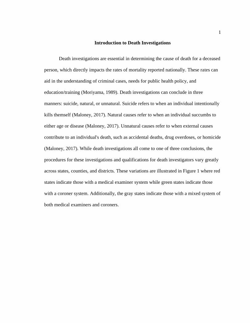
Death investigations are essential in determining the cause of death for a deceased

person, which directly impacts the rates of mortality reported nationally. These rates can

aid in the understanding of criminal cases, needs for public health policy, and

education/training (Moriyama, 1989). Death investigations can conclude in three

manners: suicide, natural, or unnatural. Suicide refers to when an individual intentionally

kills themself (Maloney, 2017). Natural causes refer to when an individual succumbs to

either age or disease (Maloney, 2017). Unnatural causes refer to when external causes

contribute to an individual's death, such as accidental deaths, drug overdoses, or homicide

(Maloney, 2017). While death investigations all come to one of three conclusions, the

procedures for these investigations and qualifications for death investigators vary greatly

across states, counties, and districts. These variations are illustrated in Figure 1 where red

states indicate those with a medical examiner system while green states indicate those

with a coroner system. Additionally, the gray states indicate those with a mixed system of

both medical examiners and coroners.

2

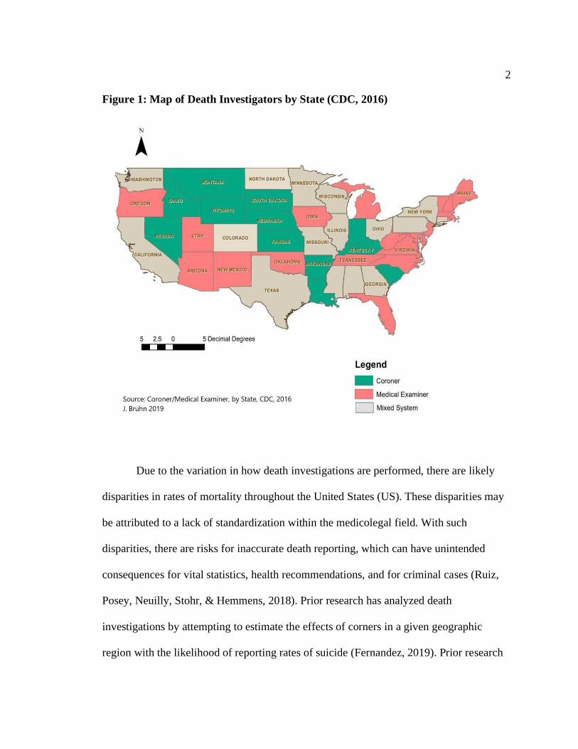
Figure 1: Map of Death Investigators by State (CDC, 2016)

Due to the variation in how death investigations are performed, there are likely

disparities in rates of mortality throughout the United States (US). These disparities may

be attributed to a lack of standardization within the medicolegal field. With such

disparities, there are risks for inaccurate death reporting, which can have unintended

consequences for vital statistics, health recommendations, and for criminal cases (Ruiz,

Posey, Neuilly, Stohr, & Hemmens, 2018). Prior research has analyzed death

investigations by attempting to estimate the effects of corners in a given geographic

region with the likelihood of reporting rates of suicide (Fernandez, 2019). Prior research

3

has also compared the minimum qualifications for both types of investigators finding a

lack of standardization and a lack of pathology requirements for coroners (Ruiz et al.,

2018). The current research examines how death investigators impact rates of homicide

and suicide across states and time.

There are two types of death investigators recognized in this study who work

under the laws of their respective states: coroners and medical examiners. These officials

work within the medicolegal system by investigating all manners of death as well as

classifying and certifying the cause of death. This research compares coroners and

medical examiners to determine if death investigators have a significant impact on

mortality rates in 35 states and the District of Columbia (DC) over 20 years (1999-2018).

4

Literature Review

This research attempts to answer the following research question: Is there a

difference in mortality rates for states requiring medical examiners for death

investigations compared to states which require coroners?

Prior research suggests there are disparities in qualifications for death

investigators across the state and county levels. These disparities include how death

investigators earn their title, training required to perform the job, how a body is examined

post-mortem, and who qualifies for death certification (Ruiz et al., 2018). With an

uninformed medicolegal system, there are risks for misinterpretation and redundancy

because there is no standardized platform for how deaths should be investigated. The

purpose of this research is to evaluate the differences in state law characteristics

regarding death investigations, its impact on rates of mortality, and how deaths are

investigated over time. The map on page seven outlines the differences across states

(CDC, 2016; Hickman, Hughes, & US Bureau of Justice Statistics, 2007). The red states

represent states using medical examiners (22 states/DC), green indicates states using

coroners (14 states), and the gray states represent states utilizing a mixed system of both

coroners and medical examiners (15 states).

The following literature review highlights characteristics of both coroners and

medical examiners while arguing educated guesses as described by General Systems

Theory may result in adverse outcomes such as improperly classified death certificates.

5

Coroners

Coroners were adopted from English Law and are the first established death

investigators of the US. Coroners refer to elected or appointed officials who investigate

the manner of death for a deceased individual. The qualifications for coroners vary

across states and jurisdictions; however, states and jurisdictions are consistent in the lack

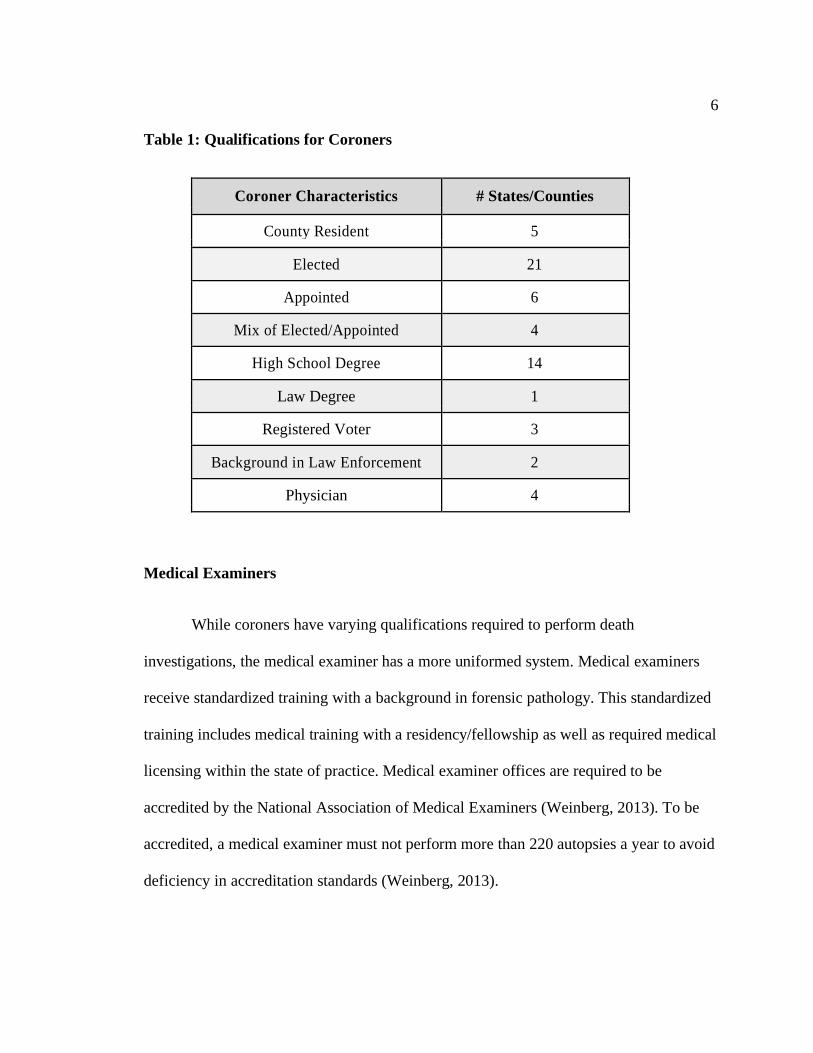
of qualification for a background in pathology. Table one highlights the various minimal

qualifications for coroners, along with the number of states/counties with these

requirements (Fernandez, 2019; Ruiz et al., 2018). As it appears on the table, many

coroners have limited medical background and learn most of their skills from on the job

training. This can prove to be problematic for many reasons because coroners are not

medically qualified to certify the cause of death for an individual; therefore, this study

argues conclusions from coroners are more likely to be inaccurate and unreliable. If the

death is improperly labeled, then this can lead to negative financial outcomes (i.e.,

nullifying life insurance, autopsy cost).

Additionally, these adverse outcomes can be associated with improper

suggestions for policies around certain types of deaths. For example, an uninformed

policy decision may manifest as a result of inaccurate homicide versus suicide rates in a

target area. This can be a result of homicides being inaccurately reported as suicides and

vice versa, causing law enforcement agencies to either neglect a prominent issue or fail in

allocating resources to the appropriate target/problem. For this reason, the lack of

medically qualified death investigators can pose a threat to public safety and risks the

diminishment of justice.

6

Table 1: Qualifications for Coroners

Coroner Characteristics # States/Counties

County Resident 5

Elected 21

Appointed 6

Mix of Elected/Appointed 4

High School Degree 14

Law Degree 1

Registered Voter 3

Background in Law Enforcement 2

Physician 4

Medical Examiners

While coroners have varying qualifications required to perform death

investigations, the medical examiner has a more uniformed system. Medical examiners

receive standardized training with a background in forensic pathology. This standardized

training includes medical training with a residency/fellowship as well as required medical

licensing within the state of practice. Medical examiner offices are required to be

accredited by the National Association of Medical Examiners (Weinberg, 2013). To be

accredited, a medical examiner must not perform more than 220 autopsies a year to avoid

deficiency in accreditation standards (Weinberg, 2013).

7

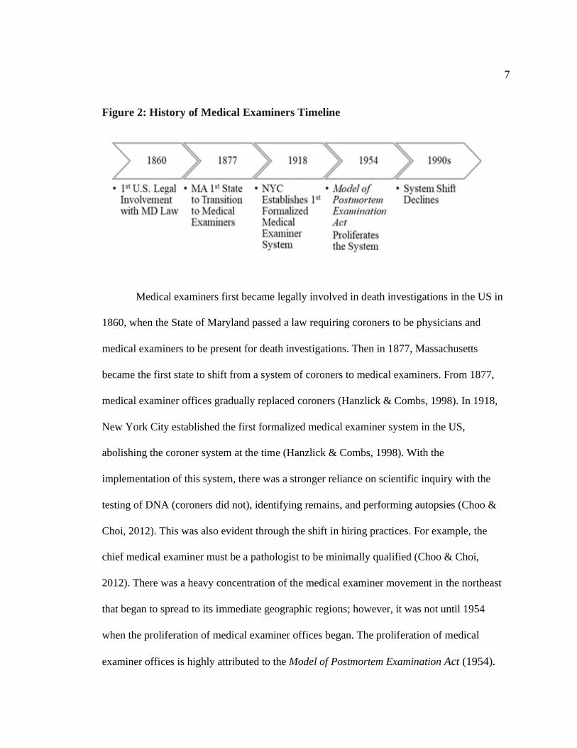
Figure 2: History of Medical Examiners Timeline

Medical examiners first became legally involved in death investigations in the US in

1860, when the State of Maryland passed a law requiring coroners to be physicians and

medical examiners to be present for death investigations. Then in 1877, Massachusetts

became the first state to shift from a system of coroners to medical examiners. From 1877,

medical examiner offices gradually replaced coroners (Hanzlick & Combs, 1998). In 1918,

New York City established the first formalized medical examiner system in the US,

abolishing the coroner system at the time (Hanzlick & Combs, 1998). With the

implementation of this system, there was a stronger reliance on scientific inquiry with the

testing of DNA (coroners did not), identifying remains, and performing autopsies (Choo &

Choi, 2012). This was also evident through the shift in hiring practices. For example, the

chief medical examiner must be a pathologist to be minimally qualified (Choo & Choi,

2012). There was a heavy concentration of the medical examiner movement in the northeast

that began to spread to its immediate geographic regions; however, it was not until 1954

when the proliferation of medical examiner offices began. The proliferation of medical

examiner offices is highly attributed to the Model of Postmortem Examination Act (1954).

8

This model outlined legislation for the development of the medical examiner death

investigation systems. The purpose of the act was to increase competency for

determining the cause of death for a deceased individual where a crime may have

occurred by adding the element of medical science to investigations. With this act, there

was a shift to a focus on forensic pathology to bring forth justice.

According to the National Commission of Forensic Science (2015), the US

required about 1,100-1,200 board-certified pathologist (medical examiners) to perform

the needed number of autopsies; however, there are a little less than 500 board-certified

pathologists registered in the US. Currently, medical examiners serve 48% of the national

population, with the highest population served in Hawai’i, New York, and Missouri. The

decline of the medical examiner's office began in the 1990s for various reasons, such as

the nature of the work and higher pay in other medical specialties. This decline of the

transition to the medical examiner system was a shift away from the movement for

medical competency in investigations set by the Model of Postmortem Examination Act

(1954). A reason for this shift may be attributed to the difficulty in changing state

constitutions with coroners written in them. For example, Georgia Constitution Article

XI (1777) states, “the senior justice on the bench shall act as chief-justice, with the clerk

of the county, attorney for the State, sheriff, coroner, constable, and the jurors when the

chief of justice is absent.”

Another reason contributing to this shift away from medical competency can be

due to the lack of resources needed to perform the job (Weinberg, 2013). In analyzing

this shift, three news articles highlighted how a lack of resources impacts the work of

9

medical examiners. The first example was in Kentucky, where the Chief State Medical

Examiner resigned in 2017 due to a lack of resources, which the resignation was later

withdrawn after a guaranteed higher budget (Eads & Desrochers, 2017). The second

example of a lack of resources impacting medical examiners was in 2017, where New

Hampshire’s Chief Medical Examiner retired, stating there was a high backlog of cases,

heavy workload, and inadequate resources to handle it (Edelstein, 2017). The third case

was found in Los Angeles, California, where the medical examiner resigned in 2016 after

being on the job for only two years, stating he did not have adequate resources necessary

to perform his job duties (Hamilton, 2016).

These resources medical examiners lack to perform their jobs adds strain to the

criminal justice system because cases cannot be adequately processed. As a result,

educated guesses as to whether to open a case for investigation or not must be made by

death investigators, which is best described by General Systems Theory.

General Systems Theory and Criminal Elements

With the lack of educational background in medicine, standards requiring

board certifications, and a background in pathology, many coroners lack the means

to produce an educated guess for death investigations. This can lead to issues such

as taking crime scenes for face value, which may require no further investigation.

This can produce invalid conclusions. This idea is much like Occam’s Razor,

where the simple solution is perceivable the soundest (Domingos, 1999). With

Occam’s Razor, there are two solutions with one being the most plausible, and the

10

other solution has more assumptions: (1) classify the death as a suicide based on

face value (2) investigate the death rejecting face value. This study argues medical

examiners are more likely to produce necessary qualities needed for death

investigations to create a more efficient system because they are better capable of

diverting from the simple solutions with scientific inquiry.

11

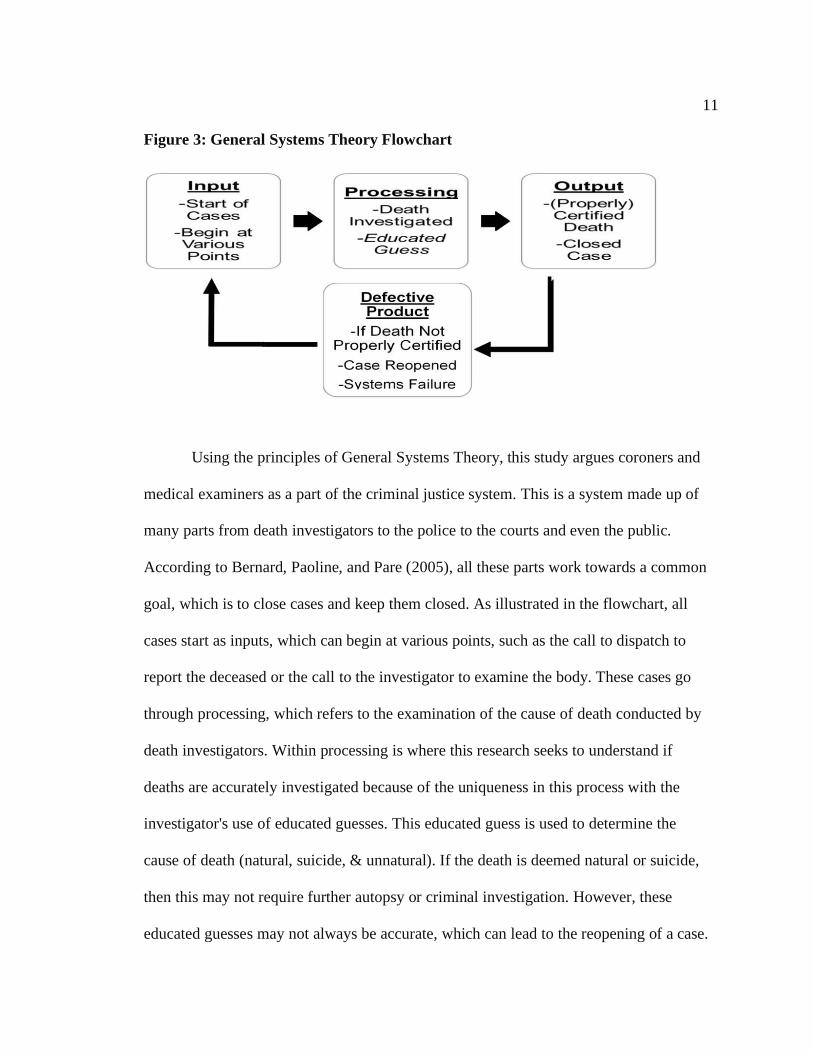
Figure 3: General Systems Theory Flowchart

Using the principles of General Systems Theory, this study argues coroners and

medical examiners as a part of the criminal justice system. This is a system made up of

many parts from death investigators to the police to the courts and even the public.

According to Bernard, Paoline, and Pare (2005), all these parts work towards a common

goal, which is to close cases and keep them closed. As illustrated in the flowchart, all

cases start as inputs, which can begin at various points, such as the call to dispatch to

report the deceased or the call to the investigator to examine the body. These cases go

through processing, which refers to the examination of the cause of death conducted by

death investigators. Within processing is where this research seeks to understand if

deaths are accurately investigated because of the uniqueness in this process with the

investigator's use of educated guesses. This educated guess is used to determine the

cause of death (natural, suicide, & unnatural). If the death is deemed natural or suicide,

then this may not require further autopsy or criminal investigation. However, these

educated guesses may not always be accurate, which can lead to the reopening of a case.

12

This reopening creates defective produce indicating systems failure, which is never a

desirable outcome.

As suggested by 40-year New York veteran homicide detective Vernon Gebreth,

the criminal element sometimes recognizes the lack of investigation around various

death methods; therefore, are likely to reconstruct the crime scene as a suicide or an

accident to avoid culpability for murder (Gebreth, Schimpff, & Senn, 2006).

Practitioners not only recognize the criminal element reconstructing scenes, but also

researchers have suggested this. Ferguson and Petherick (2016) sampled 115 crime

scenes involving death findings 16 scenes were staged suicides with the most notable

means being a firearm or hanging/asphyxiation. These findings confirm Gross (1924),

who proposed common methods of staged suicides. Gross (1924), who suggested deaths

classified as suicides by hanging, can be staged where notes can be forged while the true

method is often attributed to poisoning or strangulation (Ferguson & Petherick, 2016).

With General Systems Theory, there are pressures death investigators experience

known as forward pressures and backward pressures. Forward pressures refer to pushing a

case forward for further investigation, which helps remove fault from the investigator. For

example, if a death is labeled suicide and a follow-up investigation deemed the death as

a homicide, then this invalid death certification can be perceived as incompetence. This

inaccurate labeling requiring further investigation represents a defective output, which

directly goes against the goals of General Systems Theory to keep cases closed.

Therefore, forward pressure is a means of removing possible perceptions of

incompetency to gain more valid conclusions through further investigation. While

13

forward pressure can have positive outcomes for the investigator, it can lead to adverse

outcomes for the criminal justice system as a whole. These adverse outcomes are

associated with the progressive narrowing of the system that can be overwhelmed with

heavier caseloads, higher monetary costs, and more autopsies. Backward pressures

counter the issues from forward pressures. These backward pressures are utilized by

workers in the early stages of the system to encourage these workers to close a cases

and keep them closed rather than pushing the case forward for further investigation

(Bernard et al., 2005). Various actors from the criminal justice system will encourage

this, especially actors who are further along in the process because of the progressive

narrowing of the system. This discretion requires a certain level of competency because

the criminal justice actor must make an educated guess whether to investigate a death or

close the case. The goal for this educated guess is to create completed products, a closed

case with an appropriately labeled death certificate. However, an educated guess is

limited from on the job training and requires a more educational background.

Inconsistent Mortality Rates

A study by Voelker (1995) provides an example of systems failure through the

study of South Carolina's dual coroner and medical examiner system. The purpose of this

research was to highlight the inconsistent structure of death investigations and their

impact on various counts of death. According to Voelker's (1995) data, there were

approximately 32,000 deaths, while 410 deaths were classified as a homicide, and 487

deaths were classified as suicide; therefore, 410 deaths were followed with a criminal

14

investigation, and 487 did not. From the total suspicious deaths investigated, 40% of

these deaths were concluded as heart disease; however, these rates of heart disease

dropped significantly after a physician with medical training was elected coroner

(Voelker, 1995). This significant change in mortality rates suggests medical training

promotes a more accurate and efficient system.

Not only are death investigations, an issue for deceased adults but also deceased

infants. According to Voelker (1995), 12% of all infant deaths examined were classified

as a cause of sudden infant death syndrome without performing an autopsy. Without an

autopsy, this percentage of infant deaths cannot be confirmed as natural; therefore, no

criminal investigation is required. Without a criminal investigation, there is no

determining if a crime has been committed or not. These findings suggest a lack of

medical training for death qualifications can lead to inaccurate reporting and fewer

criminal investigations. This further supports the importance of medical training for

death investigations for more accurate reporting.

The research question is important because it serves to fill gaps in prior literature

by adding a time series element to the regression model. The work of Voelker (1995)

examined natural causes, suicide, and homicide rates with their findings suggesting

medical training impacts mortality rates; however, the model used was limited by not

having a time series element. Other prior research has examined the role of medicolegal

actors regarding geographic variation in suicide rates finding appointed medical

examiners had higher rates of homicide than elected coroners (Klugman, Condran, &

Wray, 2013). Death investigation research has examined, too, the accuracy and

effectiveness of medicolegal actors by comparing the training and qualifications of death

15

investigator officials (Fernandez, 2019). Fernandez (2019) examined the economic

effects of elected coroners and appointed medical examiners on state suicide rates. In

examining these economic effects, Fernandez (2019) found accidental deaths are 2-4%

higher in counties with elected coroners, and annual training on suicide and accidental

deaths for coroners did not affect rates of suicide. By adding a time series element, this

research can identify trends in the data while holding all other variables constant.

Research indicates that medical examiners are the more qualified death

investigators because they have a more informed educated guess and are associated

with advanced technologies/testing when compared to the coroners. Given that medical

examiners are more likely to produce valid conclusions with a properly certified death,

this research examines if there are differences in the rates of mortality given the

characteristics of the state laws. In examining the effects of death investigator on

mortality rates across states and time, two mortality hypotheses were tested:

Homicide Hypothesis: States requiring medical examiners for death investigations will

experience higher rates of homicide than states which require coroners.

Suicide Hypothesis: States requiring medical examiners for death investigations will

experience lower rates of suicide than states which require coroners.

16

Methodology

Data

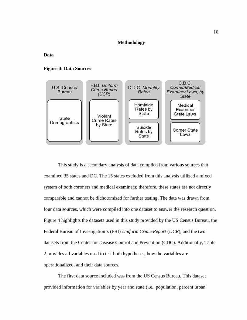
Figure 4: Data Sources

This study is a secondary analysis of data compiled from various sources that

examined 35 states and DC. The 15 states excluded from this analysis utilized a mixed

system of both coroners and medical examiners; therefore, these states are not directly

comparable and cannot be dichotomized for further testing. The data was drawn from

four data sources, which were compiled into one dataset to answer the research question.

Figure 4 highlights the datasets used in this study provided by the US Census Bureau, the

Federal Bureau of Investigation’s (FBI) Uniform Crime Report (UCR), and the two

datasets from the Center for Disease Control and Prevention (CDC). Additionally, Table

2 provides all variables used to test both hypotheses, how the variables are

operationalized, and their data sources.

The first data source included was from the US Census Bureau. This dataset

provided information for variables by year and state (i.e., population, percent urban,

17

unemployment rate, population density, percent white). Population density was

calculated every ten years; however, for all population variables examining the year

1999, the population density was assumed as the same for the 2000-2010 census. The

population density for 1999 was assumed as the following year’s census data to make

1999 more comparable due to the change in how this variable was calculated for prior

censuses.

The second dataset is sourced from the FBI UCR. This report contains crime data

for each state by year. This report accounts for crimes that were reported to the police to

which the police categorizes the crime accordingly and voluntarily reports this data

annually to the FBI. For the current research, UCR datasets from 1999-2018 were

analyzed to create a control variable accounting for violent crime rate per 100,000 for

each location examined by year.

The final two datasets were collected by the CDC. The datasets are Mortality

Rates and Coroner/Medical Examiner Laws, by state. The analysis incorporated 20 years

(1999-2018) of data recorded yearly. In addition to increasing reliability and

strengthening the power to the analysis, the data is evaluated over time allow for the

assessment of changes within each state by year and differences across states. Both

datasets collected to evaluate the differences state characteristics for death investigations

and its impact on mortality rates. The mortality data were coded by both states and the

National Center of Health Statistics using death certificates. Nonresident deaths, US

territory deaths, and fetal deaths were excluded from this dataset. These excluded

variables include nonresident aliens, nationals living abroad, residents of Puerto Rico,

Guam, the Virgin Islands, and other US territories. This excludes 46,442,365 cases.

18

Additionally, homicide deaths by terrorism were excluded from this analysis, which

accounted for 2,937 cases. All homicide deaths by terrorism were excluded from this

study because they are not directly comparable to the rates of homicide and suicide

required to answer the research question. The total number of observed death events

analyzed was 128,629,866, and these events were aggregated into the state level of

analysis by year with 720 (36 * 20) observations for the panel model. Both homicide and

suicide were converted from count data to rates for all observed states. These rates were

calculated by dividing the sum of homicides/suicides within a state per year by the total

state population multiplied by 1,000 people. Thus, the final analysis assessed changes

over time, as well as differences across states.

Dependent Variables

There are two key-dependent variables for mortality rates analyzed in this

research: homicide rates and suicide rates. These rate variables were measured per 1,000

people. They were calculated using the population of an observed location by year

divided by the total number of homicide/suicide deaths for the observed location for the

given year. Table 2 provides more information on these rates, the data source, and the

procedures for operationalization. In total, there were eight manners of death recognized

in the dataset; however, all other types of mortality will be excluded from this analysis.

The other six manners of death are excluded because they are not comparable to the types

of death examined to answer the research question. The two manners of death analyzed,

homicide and suicide, are comprised of 61 mortality categories describing the cause of

19

death. This data was collected from death certificates submitted by all states to DC. Prior

research has suggested homicides and suicides can be misclassified, which can lead to

closed cases without criminal investigation creating inaccurate conclusions for death

investigations (Gebreth et al., 2006; Ferguson & Petherick, 2016). The key dependent

variables were created from the CDC’s Mortality dataset consisting of 35 methods of

homicide and 26 methods of suicide. An example of a method of homicide in this dataset

was an assault by a blunt object, while an example of a method of suicide was intentional

self-harm by handgun discharge. This totaled 61 methods of death analyzed, which were

narrowed down to two categories for this analysis: homicide and suicide These categories

were measured/compared by year, state, and the type of death investigator.

Independent Variable

The independent variable is the type of death investigator. The coroner/medical

examiner laws, by state dataset, analyzed the differences in the death investigator laws by

state and county. There are four types of death investigation systems recognized in this

dataset: centralized medical examiner system (16 states and DC), county/district-based

medical examiner system (6 states), county-based system with a mixture of coroner and

medical examiner office (14 states), County/district/parish-based coroner system (14

states), & state medical examiner (25 states). In total, 15 states are excluded. The

analysis accounted for all revised laws regarding death investigation systems during the

20 years examined. Further information is provided in Table 2 regarding the data source

and procedures for operationalization.

20

The main independent variable analyzed is medical examiner, while coroners

were used as the comparison group. Medical examiners were selected for this analysis

because this research argues for the expansion of the medical examiner system due to the

rigorous education, accreditation, and training these professionals endured. This research

examines the two most common types of death investigators in the US: coroners &

medical examiners. All other types of death investigators have been excluded from this

analysis. A dummy variable for the independent variable was created where one refers to

states with medical examiners, and zero refers to states using coroners. The frequencies

for these investigators are highlighted in Table 4. Prior research analyzed the relationship

of death with mortality rates where finding trends with death reporting, which may be

attributed to the training death investigators undergo (Voelker, 1995). For example,

medical examiners were found to report higher rates of homicide than suicide (Klugman,

Condran, & Wray, 2013). For this reason, a dummy variable for these investigators was

generated called medical examiner. The variable was dichotomized so that zero

represents states utilizing coroners while one represents states utilizing medical

examiners.

Covariates

This study used 20 years of data from January 1, 1999-December 31, 2018.

Measures were included to account for state demographics for each year examined. Table

2 provides information about these measures regarding data sources and how the

variables were operationalized. For example, the unemployment rate was controlled for

21

because prior literature suggests an association with this rate and rates of violent crime

(Lee, Jang, Yun, Lim, Tushaus, 2010). Percent urban was also calculated and controlled

for as a state demographic variable. The percentage of the urban area within a state was

controlled for because prior research suggests more crime occurs in urban areas (Gebreth

et al., 2006). This study controlled for the rate of violent crime using UCR data as prior

research suggest there is a relationship between violent crime rates and homicides

(Gebreth et al., 2006; Ferguson & Petherick, 2016). In examining death investigators, this

study controlled for the race of the deceased as well as the racial demographics of the

state. The race of the deceased was controlled for to understand if there are interracial

effects within the mortality rates. Prior research indicates a disproportionate population

of non-whites is adversely affected by the criminal justice system (Kramer & Wong,

2019; Lautenshclager & Omori, 2018). Although non-whites experience more cumulative

disadvantages within the criminal justice system, white was selected as the examined

race while holding non-white as the reference group. White was selected because this

race accounts for the most population within each state, allowing for more

generalizability.

Additionally, this study controlled for political variables. Within the US, the two

primary political parties are the Democratic party and the Republican party. The

percentage of the Republican House party within each state by year was controlled for to

determine if political affiliation impacts mortality rates given the characteristics of the

state's death investigation laws. Political affiliation is believed to be impactful because

politicians can appoint various death investigators and have input on death investigation

financial budgeting/resources.

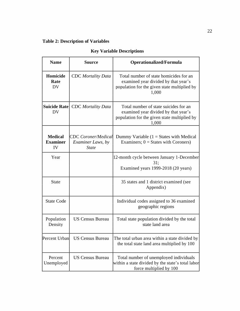
22

Table 2: Description of Variables

Key Variable Descriptions

Name Source Operationalized/Formula

Homicide CDC Mortality Data Total number of state homicides for an

Rate examined year divided by that year’s

DV population for the given state multiplied by

1,000

Suicide Rate CDC Mortality Data Total number of state suicides for an

DV examined year divided by that year’s

population for the given state multiplied by

1,000

Medical CDC Coroner/Medical Dummy Variable (1 = States with Medical

Examiner Examiner Laws, by Examiners; 0 = States with Coroners)

IV State

Year 12-month cycle between January 1-December

31;

Examined years 1999-2018 (20 years)

State 35 states and 1 district examined (see

Appendix)

State Code Individual codes assigned to 36 examined

geographic regions

Population US Census Bureau Total state population divided by the total

Density state land area

Percent Urban US Census Bureau The total urban area within a state divided by

the total state land area multiplied by 100

Percent US Census Bureau Total number of unemployed individuals

Unemployed within a state divided by the state’s total labor

force multiplied by 100

23

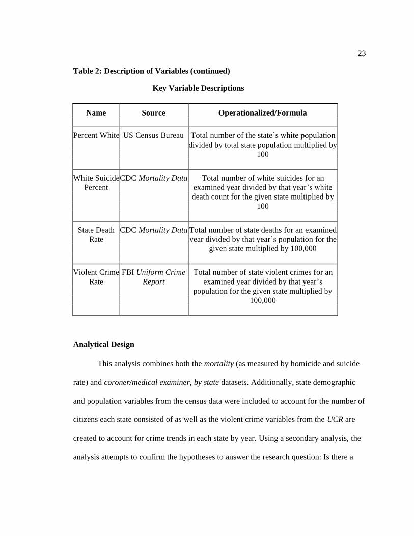
Table 2: Description of Variables (continued)

Key Variable Descriptions

Analytical Design

This analysis combines both the mortality (as measured by homicide and suicide

rate) and coroner/medical examiner, by state datasets. Additionally, state demographic

and population variables from the census data were included to account for the number of

citizens each state consisted of as well as the violent crime variables from the UCR are

created to account for crime trends in each state by year. Using a secondary analysis, the

analysis attempts to confirm the hypotheses to answer the research question: Is there a

Name Source Operationalized/Formula

Percent White US Census Bureau Total number of the state’s white population

divided by total state population multiplied by

100

White Suicide CDC Mortality Data Total number of white suicides for an

Percent examined year divided by that year’s white

death count for the given state multiplied by

100

State Death CDC Mortality Data Total number of state deaths for an examined

Rate year divided by that year’s population for the

given state multiplied by 100,000

Violent Crime FBI Uniform Crime Total number of state violent crimes for an

Rate Report examined year divided by that year’s

population for the given state multiplied by

100,000

24

difference in mortality rates for states requiring medical examiners for deaths compared

to states requiring coroners?

In total the analysis covers the years 1999-2018 (t = 20) and 36 states/district (i =

720). The models utilized in this study replicated Lester’s (1999) study in Hong Kong,

examining the effects of marriage, birth, and unemployment rates on suicide and

homicide rates. Using a time series model, Lester (1999) researched the period from 1976

to 1992 found no association between the variables measured as rates per 10,0000

population; therefore, suicide and homicide were not predicted by rates of marriage,

birth, and unemployment. This research attempted to identify predictors of homicide and

suicide using a time-series design in examining the effects of type of death investigator

on these rates of mortality.

Using a Prais-Winsten regression model with panel-corrected standard errors, this

research analyzed the variations of how states investigate deaths over time. To calculate

panel-corrected standard errors (PCSE), all disturbances within the dataset are assumed

heteroskedastic and correlated across panels (Blackwell, 2005). When analyzing rates of

homicide and suicide, the impacts are often correlated with the previous year as events

are not isolated to one year (i.e., violent crime rate). Because there is autocorrelation

within the models, Prais-Winsten Regression was used (Kmenta, 1997). This type of

linear regression model uses a generalized least-squares method rather than ordinary

least-squares accounting for correlation within the model (Kmenta, 1997).

Panel models can suffer from several specification errors that can lead to invalid

results. One of the key items to test for is if the model is suffering from omitted variable

bias (OVB). OVB is present when unobserved time-dependent or unit-dependent

25

variables that are correlated with the error in the model. A Hausman test can be used to

determine if OVB is present. The test confirmed that for both homicide and suicide rates,

OVB was present. To correct for this, the current research implements a panel (cross-

sectional time-series) regression design using the Prais-Winsten regression model with

panel-corrected standard errors. Additionally, to correct for serial correlation, the model

utilized an autocorrelation term (AR1) of one year. Implementing an AR1 term correlates

each year with the previous year. By using an AR1 term, one year of data was removed.

This year was 1999 as it had nothing to be correlated with due it being the first year

observed within the dataset; therefore, 1999 was used as a control for serial correlation

for all mortality rate models. The specification allowed the model to estimate the effects

of the time-invariant variables used to answer the research question. An additional

Hausman test of the model indicates that this model is not likely to suffer from OVB.

The four combined datasets were used to administer all tests in this research.

The panel variable for all regression models was state code (see Table 2 for

operationalization). The time variable was specified as a year. The period examined to

test both hypotheses is from January 1, 1999-December 31, 2018 (t = 20). By adding

the element of time to the model, the study can observe changes in mortality rates over

a span of years, given the type of death investigator required by the given state. Using

multiple regressions, the model estimated the effects of the type of death investigator

required by the state on mortality rates while holding all other variables constant. Each

mortality rate for all states and years were tested independently to isolate the impact of

the type of death investigator. Six regression models were developed to explain the

variation within the dataset. The two full models using the suicide rate and homicide

26

rate as the dependent variables were compared to determine if medical examiners report

more homicides than suicides.

The model uses a pairwise specification. By implementing pairwise into the model,

the model can account for all variable observations with non-missing pairs. This helped

saved observations such as demographic mortality rates (i.e., white homicide percent) due

to the non-reporting of sensitive racial demographics for criminal/private cases. With the

pairwise specification, the model loses statistical power by making assumptions out of the

missing data. These assumptions can lead to invalid results; however, the omitted data was

low, minimizing any concerns for possible invalidation.

The overall goal was to inform of the cross-sectional effects of the type of death

investigator across mortality rates and its variation over time (t = 20). The analytical

technique for this research called for repeated observations of the type of death

investigator measured by states over time. By repeating observations of the type of

death investigator by states over time, estimates for projected mortality rates were

calculated based on prior data given certain state law characteristics.

27

Results

Descriptive Statistics

Table 3 shows the descriptive statistics for all variables included in the model that

analyzes the 36 observed states/districts during the 20 years examined. The mean for the

homicide rate was 5.54 (N = 720; SD = 4.38) per 1,000 population per year. The mean

for the suicide rate was 14.64 (N = 720; SD = 4.40).

In addition to the mortality variables, the table highlights the descriptive statistics

of the control variables. There are five control variables with complete observations.

Population density has a mean of 457.88 (N = 720; SD = 1643.74). Population density

has a mean of 457.88 (N = 720; SD = 1643.74). Percent urban has a mean of 71.26 (N =

720; SD = 15.59). Percent unemployed has a mean of 5.68 (N = 720; SD = 5.49). Percent

white has a mean of 83.89 (N= 720; SD= 14.64). State death rate has a mean of 867.08

(N = 720; SD = 132.09). Violent crime rate has a mean of 420.81 (N = 720; SD =

242.98).

Within Table 3, there is an indication that three variables are have omitted

observations. These variables are percent Republican House (N = 644; SD = 28.94),

white homicide percent (N = 674; SD = 36.81), and white suicide percent (N = 7.17; SD

= 7.76).

28

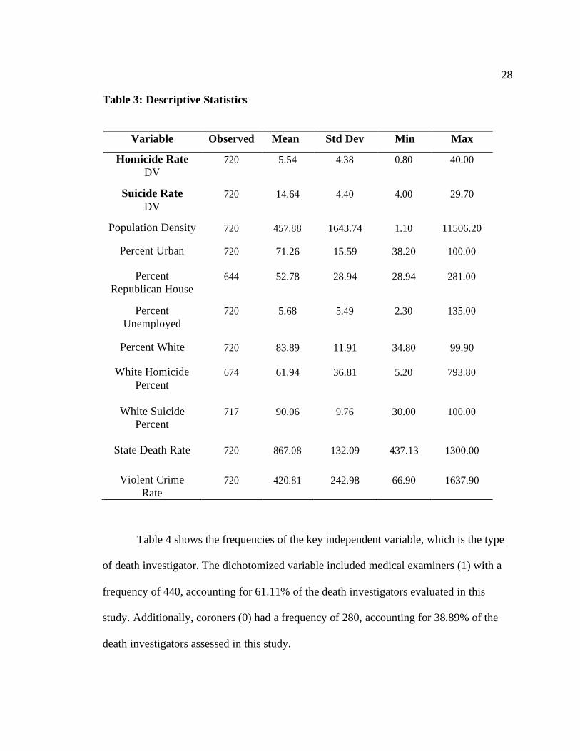
Table 3: Descriptive Statistics

Table 4 shows the frequencies of the key independent variable, which is the type

of death investigator. The dichotomized variable included medical examiners (1) with a

frequency of 440, accounting for 61.11% of the death investigators evaluated in this

study. Additionally, coroners (0) had a frequency of 280, accounting for 38.89% of the

death investigators assessed in this study.

Variable Observed Mean Std Dev Min Max

Homicide Rate 720 5.54 4.38 0.80 40.00

DV

Suicide Rate 720 14.64 4.40 4.00 29.70

DV

Population Density 720 457.88 1643.74 1.10 11506.20

Percent Urban 720 71.26 15.59 38.20 100.00

Percent 644 52.78 28.94 28.94 281.00

Republican House

Percent 720 5.68 5.49 2.30 135.00

Unemployed

Percent White 720 83.89 11.91 34.80 99.90

White Homicide 674 61.94 36.81 5.20 793.80

Percent

White Suicide 717 90.06 9.76 30.00 100.00

Percent

State Death Rate 720 867.08 132.09 437.13 1300.00

Violent Crime 720 420.81 242.98 66.90 1637.90

Rate

29

Table 4: Frequency Table for Death Investigators

Death Investigator Type Frequency Percent

0 (Coroner) 280 38.89

1 (Medical Examiner) 440 61.11

Total 720 100.00

Homicide Rates and Medical Examiners

This research hypothesized medical examiners report higher rates of homicides

than coroners. Three regression models were developed to analyze the impact of medical

examiners on homicide rates. All three Prais-Winsten Regression models for homicide

rates are highlighted in Table 5. The results of the first model reject the null hypothesis

because medical examiners are associated with higher rates of homicide. When other

variables are controlled within the full model, the results indicate an increase of medical

examiners is associated with a decrease in homicide rates. Therefore, the full model fails

to reject the null hypothesis as medical examiners are associated with lower rates of

homicide. The details of both models are discussed below.

30

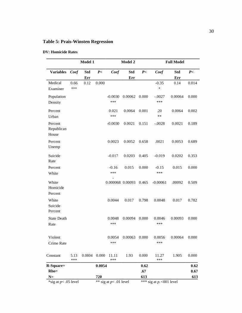
Table 5: Prais-Winsten Regression

DV: Homicide Rates

Model 1 Model 2 Full Model

Variables Coef Std P< Coef Std P< Coef Std P<

Err Err Err

Medical 0.66 0.12 0.000 -0.35 0.14 0.014

Examiner *** *

Population -0.0030 0.00062 0.000 -.0027 0.00064 0.000

Density *** ***

Percent 0.021 0.0064 0.001 .20 0.0064 0.002

Urban *** **

Percent -0.0030 0.0021 0.151 -.0028 0.0021 0.189

Republican

House

Percent 0.0023 0.0052 0.658 .0021 0.0053 0.689

Unemp

Suicide -0.017 0.0203 0.405 -0.019 0.0202 0.353

Rate

Percent -0.16 0.015 0.000 -0.15 0.015 0.000

White *** ***

White

-

0.000068 0.00093 0.465 -0.00061 .00092 0.509

Homicide

Percent

White 0.0044 0.017 0.798 0.0048 0.017 0.782

Suicide

Percent

State Death 0.0048 0.00094 0.000 0.0046 0.00093 0.000

Rate *** ***

Violent 0.0054 0.00063 0.000 0.0056 0.00064 0.000

Crime Rate *** ***

Constant 5.13 0.0804 0.000 11.11 1.93 0.000 11.27 1.905 0.000

*** *** ***

R-Square= 0.0054 0.62 0.62

Rho= .67 0.67

N= 720 613 613

*sig at p< .05 level ** sig at p< .01 level *** sig at p.<001 level

31

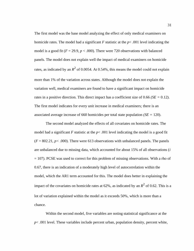
The first model was the base model analyzing the effect of only medical examiners on

homicide rates. The model had a significant F statistic at the p< .001 level indicating the

model is a good fit (F = 29.9, p < .000). There were 720 observations with balanced

panels. The model does not explain well the impact of medical examiners on homicide

rates, as indicated by an R2 of 0.0054. At 0.54%, this means the model could not explain

more than 1% of the variation across states. Although the model does not explain the

variation well, medical examiners are found to have a significant impact on homicide

rates in a positive direction. This direct impact has a coefficient size of 0.66 (SE = 0.12).

The first model indicates for every unit increase in medical examiners; there is an

associated average increase of 660 homicides per total state population (SE = 120).

The second model analyzed the effects of all covariates on homicide rates. The

model had a significant F statistic at the p< .001 level indicating the model is a good fit

(F = 802.21, p< .000). There were 613 observations with unbalanced panels. The panels

are unbalanced due to missing data, which accounted for about 15% of all observations (i

= 107). PCSE was used to correct for this problem of missing observations. With a rho of

0.67, there is an indication of a moderately high level of autocorrelation within the

model, which the AR1 term accounted for this. The model does better in explaining the

impact of the covariates on homicide rates at 62%, as indicated by an R2 of 0.62. This is a

lot of variation explained within the model as it exceeds 50%, which is more than a

chance.

Within the second model, five variables are noting statistical significance at the

p< .001 level. These variables include percent urban, population density, percent white,

32

state death rate, and violent crime rate. Percent urban has a positive, significant impact on

medical examiners. The coefficient size is 0.021 (SE = 0.0064). Thus, when all variables

are controlled for, for every unit increase in percent urban, there is an associated average

increase of about two homicides per total state population (SE = 6.4). Conversely,

population density has a negative impact on homicide rates suggesting as population

density increases, homicide rates decrease. This is indicated by the coefficient size of

population density, which is -0.0030 (SE = 0.00062). Therefore, controlling for all other

variables, for every unit increase in population density, there is an average decrease of

three homicides per total state population (SE = 0.62). This direction is also followed by

percent white. Percent white has a coefficient size of -0.16 (SE = 0.015). This indicates

for every unit increase in the percentage of the white population within a state; there is an

associated average decrease of 160 homicides per total state population when all other

variables are held constant (SE= 15). State death rate and violent crime rate are consistent

with the literature in its association with rates of homicide. Both rates have a significant

positive impact on homicide rates. The coefficient size for the state death rate is 0.0048

(SE = 0.00094). This suggests for every unit increase in state death rates; there is an

associated average increase of about five homicides per total state population when all

other variables are held constant (SE = 0.94). Lastly, the second model indicates when

the other covariates are controlled for, for every unit increase in violent crime rate, there

is an associated average increase of about five homicides per total state population when

all other variables are controlled for (SE = 0.63). This is indicated by a coefficient size of

0.0054 (SE = 0.00063).

33

The full model analyzed the effects of all variables, including medical examiners

on homicide rates. The model had a significant F statistic at the p< .001 level (F =

802.21, p< .000). There were 613 observations with unbalanced panels due to the

removal of about 15% of all observations. As with the second model, PCSE was used to

correct for this problem. With a rho of 0.67, the model has a moderately high level of

autocorrelation, which is slightly higher than the previous. The AR1 accounted for this

autocorrelation. The model maintains its level of explanation of the impacts of all

variables on homicide rates at 62%, as indicated by an R2 of 0.62. By adding medical

examiner into the full model, medical examiners do not increase the level of variation is

explained across states within the model. Six variables are noting statistical significance

at various levels within the full model. These variables include medical examiners,

population density, percent urban, percent white, state death rate, and violent crime rate.

Within the full model, medical examiners lost a level of significance from the p<

.001 level to p< .01 (p< .014) but remains a significant predictor of homicide rates. The

model suggests a negative impact between medical examiners and homicide rates. These

results are unlike the first model because medical examiners are now associated with a

decrease in rates of homicide. This is indicated by the coefficient size of medical examiners,

which is -0.35 (SE = 0.14). When all other variables are controlled for, for every unit

increase in medical examiners, there is an associated average decrease of 350 homicides per

total state population (SE = 140). Percent urban has a significantly positive impact on

homicide rates (p< .002). Although percent urban loses a level of significance from the p<

.001 level, the variable remains impactful on rates of homicide across states. The coefficient

34

size for percent urban is slightly more than the previous model at 0.20 (SE = 0.0064). Thus,

controlling for all other variables, for every unit increase in percent urban, homicides

increase, on average, 200 per total state population when holding all other variables

constant (SE = 6.4). The second model suggests a negative impact observed with

population density and homicide rates (p< .000). This means when population density

increases, homicide rates decrease. The coefficient size for population density is slightly

smaller than the second model at -0.0027 (SE = 0.00064). Thus, for every unit increase

in population density, there is an average decrease of 270 homicides per total state

population when holding all other variables constant (SE = 0.64). A significant negative

impact is also observed with percent white and homicide rates (p<.000). The coefficient

size for percent white is -0.15 (SE = 0.015). This indicates for every unit increase in the

percentage of whites, and there is an associated average decrease of 150 homicides per

total state population when holding all other variables constant. Consistent with prior

literature, the state death rate has a significantly positive impact on homicide rates (p<

.000). The coefficient size for the state death rate is 0.0046, which is slightly less than

the second model (SE = 0.00093). For every unit increase in state death rates, there is an

associated average decrease of about five homicides per total state population when

holding all other variables constant (SE = 0.93). Also, consistent with prior literature,

the violent crime rate has a direct impact on homicide rates. The coefficient size for the

violent crime rate is 0.0056, which is slightly more than the second model (SE =

0.00064). This indicates for every unit increase in violent crime rates, and there is an

35

associated an average increase of about six homicides per total state population when

holding all other variables constant (SE = 0.064).

Suicide Rates and Medical Examiners

This research hypothesized medical examiners report lower rates of suicides than

coroners. Three regression models were developed to analyze the impact of medical

examiners on suicide rates (see Table 5). The models replicate the design of the three

homicide rates models in terms of the F statistic, R2, rho, and with the AR1

autocorrelation. Medical examiners in the full model are not statically significant

(p<.554). The results indicate failure to reject the null hypothesis as the results cannot

suggest that states who utilize medical examiners are associated with lower rates of

suicide.

36

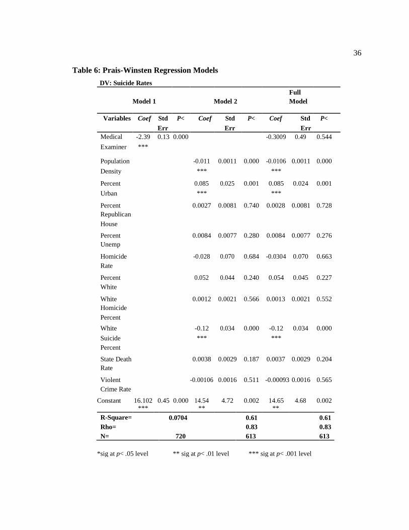
Table 6: Prais-Winsten Regression Models

DV: Suicide Rates

Model 1 Model 2

Full

Model

Variables Coef Std P< Coef Std P< Coef Std P<

Err Err Err

Medical -2.39 0.13 0.000 -0.3009 0.49 0.544

Examiner ***

Population -0.011 0.0011 0.000 -0.0106 0.0011 0.000

Density *** ***

Percent 0.085 0.025 0.001 0.085 0.024 0.001

Urban *** ***

Percent 0.0027 0.0081 0.740 0.0028 0.0081 0.728

Republican

House

Percent 0.0084 0.0077 0.280 0.0084 0.0077 0.276

Unemp

Homicide -0.028 0.070 0.684 -0.0304 0.070 0.663

Rate

Percent 0.052 0.044 0.240 0.054 0.045 0.227

White

White 0.0012 0.0021 0.566 0.0013 0.0021 0.552

Homicide

Percent

White -0.12 0.034 0.000 -0.12 0.034 0.000

Suicide *** ***

Percent

State Death 0.0038 0.0029 0.187 0.0037 0.0029 0.204

Rate

Violent -0.00106 0.0016 0.511 -0.00093 0.0016 0.565

Crime Rate

Constant 16.102 0.45 0.000 14.54 4.72 0.002 14.65 4.68 0.002

*** ** **

R-Square= 0.0704 0.61 0.61

Rho= 0.83 0.83

N= 720 613 613

*sig at p< .05 level ** sig at p< .01 level *** sig at p< .001 level

37

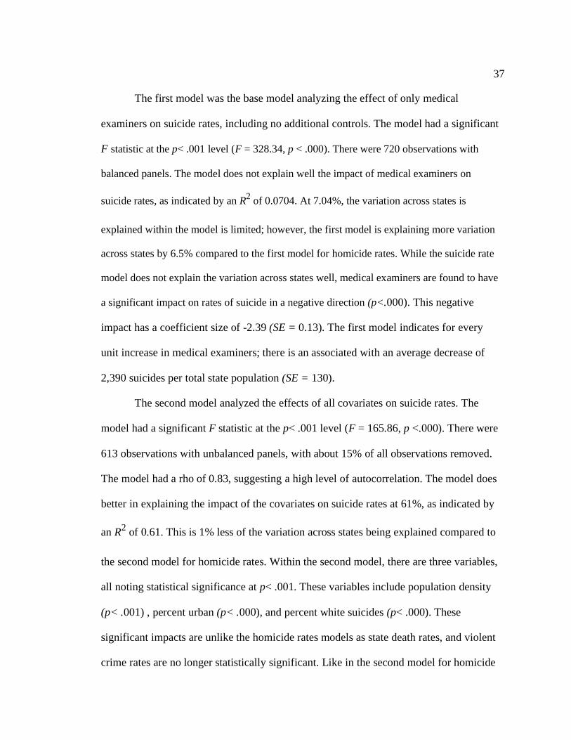
The first model was the base model analyzing the effect of only medical

examiners on suicide rates, including no additional controls. The model had a significant

F statistic at the p< .001 level (F = 328.34, p < .000). There were 720 observations with

balanced panels. The model does not explain well the impact of medical examiners on

suicide rates, as indicated by an R2 of 0.0704. At 7.04%, the variation across states is

explained within the model is limited; however, the first model is explaining more variation

across states by 6.5% compared to the first model for homicide rates. While the suicide rate

model does not explain the variation across states well, medical examiners are found to have

a significant impact on rates of suicide in a negative direction (p<.000). This negative

impact has a coefficient size of -2.39 (SE = 0.13). The first model indicates for every

unit increase in medical examiners; there is an associated with an average decrease of

2,390 suicides per total state population (SE = 130).

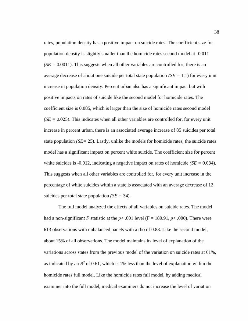
The second model analyzed the effects of all covariates on suicide rates. The

model had a significant F statistic at the p< .001 level (F = 165.86, p <.000). There were

613 observations with unbalanced panels, with about 15% of all observations removed.

The model had a rho of 0.83, suggesting a high level of autocorrelation. The model does

better in explaining the impact of the covariates on suicide rates at 61%, as indicated by

an R2 of 0.61. This is 1% less of the variation across states being explained compared to

the second model for homicide rates. Within the second model, there are three variables,

all noting statistical significance at p< .001. These variables include population density

(p< .001) , percent urban (p< .000), and percent white suicides (p< .000). These

significant impacts are unlike the homicide rates models as state death rates, and violent

crime rates are no longer statistically significant. Like in the second model for homicide

38

rates, population density has a positive impact on suicide rates. The coefficient size for

population density is slightly smaller than the homicide rates second model at -0.011

(SE = 0.0011). This suggests when all other variables are controlled for; there is an

average decrease of about one suicide per total state population (SE = 1.1) for every unit

increase in population density. Percent urban also has a significant impact but with

positive impacts on rates of suicide like the second model for homicide rates. The

coefficient size is 0.085, which is larger than the size of homicide rates second model

(SE = 0.025). This indicates when all other variables are controlled for, for every unit

increase in percent urban, there is an associated average increase of 85 suicides per total

state population (SE= 25). Lastly, unlike the models for homicide rates, the suicide rates

model has a significant impact on percent white suicide. The coefficient size for percent

white suicides is -0.012, indicating a negative impact on rates of homicide (SE = 0.034).

This suggests when all other variables are controlled for, for every unit increase in the

percentage of white suicides within a state is associated with an average decrease of 12

suicides per total state population (SE = 34).

The full model analyzed the effects of all variables on suicide rates. The model

had a non-significant F statistic at the p< .001 level (F = 180.91, p< .000). There were

613 observations with unbalanced panels with a rho of 0.83. Like the second model,

about 15% of all observations. The model maintains its level of explanation of the

variations across states from the previous model of the variation on suicide rates at 61%,

as indicated by an R2 of 0.61, which is 1% less than the level of explanation within the

homicide rates full model. Like the homicide rates full model, by adding medical

examiner into the full model, medical examiners do not increase the level of variation

39

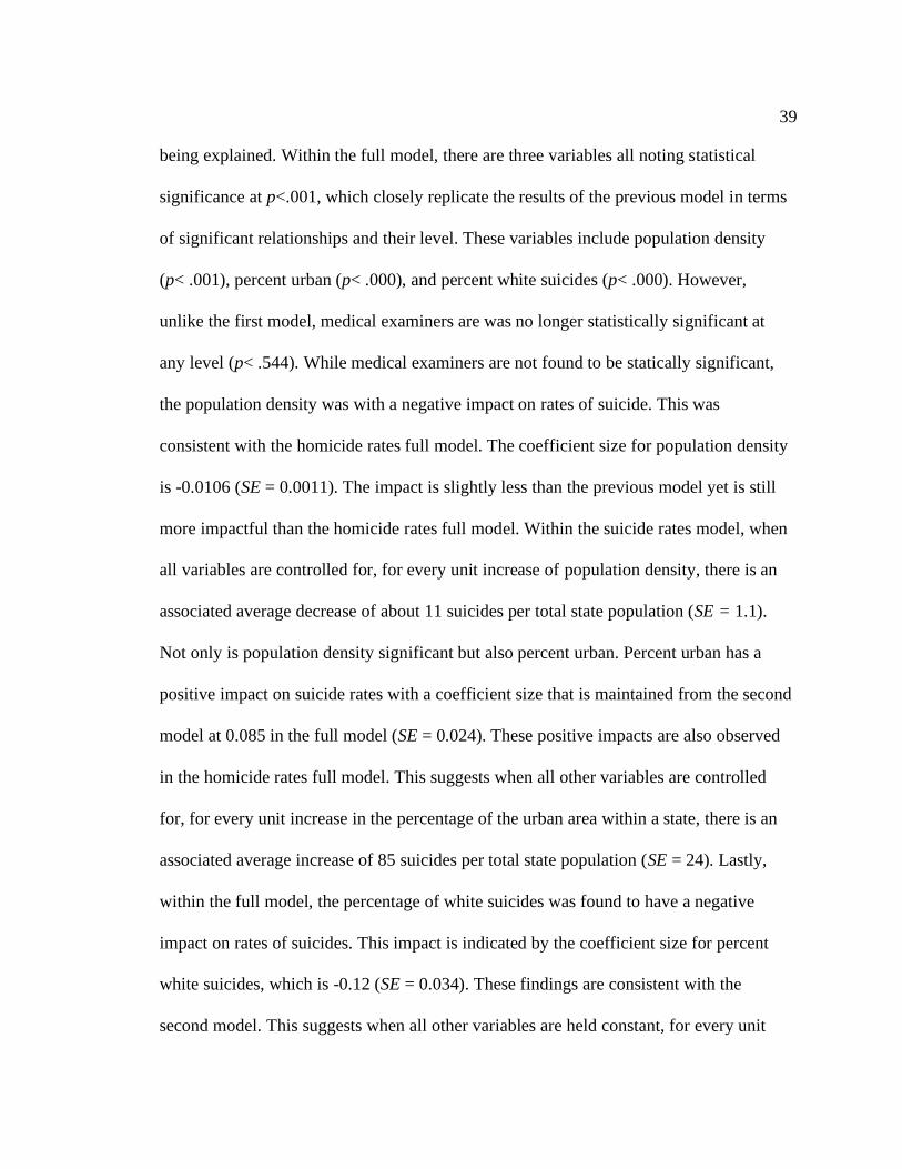
being explained. Within the full model, there are three variables all noting statistical

significance at p<.001, which closely replicate the results of the previous model in terms

of significant relationships and their level. These variables include population density

(p< .001), percent urban (p< .000), and percent white suicides (p< .000). However,

unlike the first model, medical examiners are was no longer statistically significant at

any level (p< .544). While medical examiners are not found to be statically significant,

the population density was with a negative impact on rates of suicide. This was

consistent with the homicide rates full model. The coefficient size for population density

is -0.0106 (SE = 0.0011). The impact is slightly less than the previous model yet is still

more impactful than the homicide rates full model. Within the suicide rates model, when

all variables are controlled for, for every unit increase of population density, there is an

associated average decrease of about 11 suicides per total state population (SE = 1.1).

Not only is population density significant but also percent urban. Percent urban has a

positive impact on suicide rates with a coefficient size that is maintained from the second

model at 0.085 in the full model (SE = 0.024). These positive impacts are also observed

in the homicide rates full model. This suggests when all other variables are controlled

for, for every unit increase in the percentage of the urban area within a state, there is an

associated average increase of 85 suicides per total state population (SE = 24). Lastly,

within the full model, the percentage of white suicides was found to have a negative

impact on rates of suicides. This impact is indicated by the coefficient size for percent

white suicides, which is -0.12 (SE = 0.034). These findings are consistent with the

second model. This suggests when all other variables are held constant, for every unit

40

increase of the percentage of white suicides, there is an associated average decrease in

120 suicides per total state population (SE = 34).

41

Discussion

In a national, cross-sectional time-series analysis of state death investigation

policies and its impact on mortality rates, this research answered: Is there a difference

in mortality rates for states requiring medical examiners for death investigations

compared to states which require coroners? As the results indicate, no, medical

examiners do not report more homicides than coroners, nor do they report fewer

suicides than corners in the full models. The full models represent the models that are

the most theoretically sound. These key findings of this research were unexpected,

along with the various nuances inside models in terms of levels of explanation and the

impacts of variables on rates of mortality. This discussion attempts to bridge the gaps of

these unexpected findings, followed by limitations of this study and avenues for future

research as well as policy.

First, medical examiners within both models are poor measures for explaining the

variation of mortality rates across states. Prior research suggests death investigators can

be impactful on rates mortality such as suicide, yet this concept is not supported by the

current findings (Klugman et al., 2013). The model analyzing homicide rates with just

medical examiner is limited in explaining only 0.54% of the variation across states. This

is a low level of what is being explained across states within the first model. This finding

was a surprise because the initial idea was death investigators could explain the variation

across states well, yet this was not the case. When the covariates were added in the full

model, the explanation of the variation across states within the model increased to 62%.

For this reason, it appears that other variables are the driving forces of homicide rates and

42

not death investigators. Within the compared models, medical examiners significantly

decreased in its coefficient value and its direction of impact. This is showing that other

variables are having greater impacts on rates of homicide. The model analyzing suicide

rates just medical examiner is also limited in explaining the variations across states at

7.06%. While this value is low in terms of its level of explanation, the first model for

suicide rates does better than explaining the first model for homicide rates. When other

variables are considered, the level of explanation of the variation across states increases

to 61%. This is slightly lower than the level of explanation than the full model from

homicide rates, in which these results were unexpected. The expectation was that the

suicide rates full model would do better in explaining the variability than the homicide

rates full model because medical examiners explained more of the variation across states

in the initial model for suicide rates. One thing to note about the model, including

suicides, is medical examiners are no longer significant when included in the full model,

which implies there are other measures are contributing to the impact on suicide rates.

There are two proposed reasons why medical examiners are associated with

lower rates of homicide, both concerned with resources. These concerns can range from

increased resources in areas for medical examiners or lack of resources for medical

examiners to perform their job.

Increased resources may attribute to why medical examiners may report fewer

homicides. This is because areas utilizing medical examiners require higher budgets to

cover the costs of all scientific analysis as well as medical facilities. With higher budgets

allocated towards death investigations, assumptions can be made that more budgeting is

dedicated to public health and policy initiatives (Weinberg, Weeden, Weinberg, &

43

Fowler, 2013). Therefore, homicides in areas with medical examiners may be less likely

due to prevention from public health policies and police enforcement. Additionally,

medical examiners may report more homicides than suicides compared to coroners

because of their location. States who only utilize medical examiners may be

concentrated in areas with higher rates of violent crime such as Louisiana or North

Carolina (FBI UCR, 2018). Therefore, these higher rates of violent crime concentrated

in certain locations can have direct impacts on rates of homicide, resulting in higher

reports.

On the other hand, a lack of resources may be contributing to the lower rates of

homicide reported by medical examiners. Based on prior literature, this research proposes

the findings suggesting homicide rates are lower in states using medical examiners can be

attributed to a lack of resources. These resources refer to both human capital and

monetary costs. As the 2018 report from the National Commission of Forensic Science

suggests, the US has more deaths requiring autopsies than some can perform them

(Weinberg, 2013). Furthermore, autopsies can pose a financial burden on the state due to

the costs associated with body examination/testing (Eads & Desrochers, 2017; Edelstein,

2017; Hamilton, 2016). These issues involving a lack of resources can cause strain on the

system leading to backward pressures (Bernard et al., 2005). Therefore, a lack of

resources can explain why medical examiners do not report more homicides than

coroners.

While the results do not indicate medical examiners as the better investigator, this

study speculates medical examiners are better suited for the investigator position.

Medical examiners are arguably the better investigator as they are associated with more

44

use of scientific inquiry. This inquiry involves testing bodily fluids, DNA, and

performing autopsies. With higher use of scientific inquiry, medical examiners should

have better informed educated guesses bringing forth more valid conclusions. While a

more thorough investigation may produce more valid results, this can also have adverse

outcomes on the state’s death investigation system. These adverse outcomes are

associated with the high financial costs required for the medical examiner

facility/equipment and medical examiner's wages. With these high costs, implementing a

medical examiner system in specific areas like rural areas can lead to backward

pressures. These backward pressures can result in systems failure, which can cause an

ineffective medical examiner system within the jurisdiction. Therefore, it is important for

policymakers to properly allocate funding for death investigations to reduce the strain

experienced by the investigators. With reduced strain, the system should experience less

backward pressures creating a more effective death investigation system.

Limitations

There are several notable limitations of this study that should be considered. First,

this study only examines states who utilize either a coroner or a medical examiner

system. This requirement excludes 15 states utilizing a mixed system. By excluding these

states, this study cannot account for differences in impacts across states with a mixed

system. Additionally, the models lose observations and generalizability.

Limitations are also found within the violent crime dataset sourced from the FBI’s

UCR. This data provides limitations to the measure as it only accounts for violent crimes

45

reported voluntarily by police departments to the FBI and did not account for the dark figure

of crime (De Castelbajac, 2014). This dark figure includes crimes not reported to the

police as well as crimes reported to the police but not reported to the FBI by police

departments.

There are not only limitations to how the rate of violent crime is measured but

also with the variable coroners. This study fails to acknowledge the differences in these

coroner requirements. As noted in Table 1, there are four jurisdictions requiring coroners

to be physicians as a minimum job requirement. An argument can be made that coroners

who are physicians are more qualified for an informed, educated guess as described by

General Systems Theory. If coroners in some jurisdictions have an informed, educated

guess, then they resemble similar characteristics of medical examiners. This may

attribute to why both hypotheses were failed to be rejected.

Another notable limitation of the research is the unit of analysis. Counties were

the intended unit of analysis for the current study as they can produce better results;

however, limited information and online resources were providing the laws/policies of

how each county investigates deaths. Therefore, the unit of analysis was adapted to states,

which lowered the observation count, yet the model was able to maintain its statistical

power. Additionally, this research was limited because of a change in the period

examined. The original intent was to analyze mortality rates from 1968-2018; however,

the CDC mortality data was limited to 1999-2018. By excluding 30 years of mortality

data, the models lose more than 1,000 observations resulting in a loss of statistical power.

Furthermore, the study was not able to account for any changes in death investigation

46

laws because of the limited time frame examined. Without the inclusion of changes in

death investigation laws as to who investigates, this study could not account for if states

experienced different rates of mortality post-law change.

Lastly, there are limitations in the measurement of how the CDC calculated

mortality rates because these rates only include resident deaths and do not account for

nonresident and US territory deaths. The population of the excluded accounts for

46,442,365 cases. Nonresidents in prior research have been associated with higher rates

of homicide and suicide; therefore, research needs to cover this population of people as

they are directly affected by the death investigation policies this research evaluates.

Future Research

The limitations of this study provide avenues for future research. Future research

should replicate this panel model design by increasing the observed years and analyzing

the data at the county unit level of analysis. By changing the unit of analysis from the

state level to county level and expanding the interval of time observed, the model can

explain more of the variation between mortality rates and death investigator types. This

research should include measures for financial budgeting as prior literature suggest this is

an issue for the medicolegal field (Eads & Desrochers, 2017; Edelstein, 2017; Hamilton,

2016). An additional control this study should consider is the number of autopsies

performed in a year by a state. Autopsies are associated with a high financial burden on

47

the states due to the costs for scientific inquiry and incomes associated with pathologists

who perform the autopsies. Research like this should be conducted because this study

proposes medical examiners report lower rates of homicide because they are in areas

that have either increased resources or a lack of resources needed to perform their job.

By controlling for budget, this type of research design can indicate if homicide rates are

associated with financial budgeting.

Future research should also explore the 14 states utilizing the coroner system.

This measure provided a major limitation to the present research as this research could

not control for coroners who are medically trained. A design examining only coroner

states should dichotomize the death investigator measure. This type of dummy variable

can isolate the impacts of medically trained coroners to examine if this qualification

impacts rates of mortality.

Lastly, future research should also consider adapting the model to an interrupted

time-series design examining states who adopted medical examiners and no longer use

the coroner system. The rate of mortality along with other controlling variables should

be examined within these states before the policy of adopting medical examiners was

enacted and after the policy of adopting medical examiners was enacted to determine if

death investigator policies are indicative of rates of mortality.

Policy Implications

Implications based on this study's findings are limited due to the need for

further evaluation. As to no surprise, an increase in rates of violent crimes was

48

associated with an average increase of about six homicides per state. These results

suggest the criminal justice system should continue to focus their efforts towards

decreasing rates of violent crime to decrease rates of homicide. Specifically, this can be

done through various policy initiatives such as Problem-Orientated-Policing to identify

the state's violent crime disorder to amend these issues. This should, in theory, decrease

homicide rates experienced across states.

Implications for policy are not only with increasing law enforcement resources to

reduce violent crime, but there are also implications for urbanized areas. The results of

both mortality models indicate for every unit increase in the percentage of the urban area

within a state; there is an associated increase of both homicides and suicides. This

indicates more measures must be taken by jurisdictions in urbanized areas. A suggested

measure to reduce rates of suicides urbanized areas can implement is providing easily

accessible/affordable mental health services to the general public. Furthermore, actions

can be taken by law enforcement agencies in urbanized areas with increased training in

conflict resolution and creating task force teams such as gangs or gun violence. With

increased resources and training in urbanized areas, rates of homicides and suicides

should decrease; however, further research will be required to evaluate these impacts.

While implications cannot be made about who more accurately reports mortality

rates, this study holds it is important to continue to improve the death investigation

system to have positive impacts on public health and criminal justice. These

improvements can come in both the form of human capital and financial budgeting. As

previously proposed, a lack of resources may contribute to why medical examiners are

49

associated with fewer homicides. Human capital is an issue death investigations face

because there are not enough qualified people to perform autopsies the needed number

of autopsies each year.

50

Conclusion

In this study, it was hypothesized medical examiners would report higher rates of

homicides and lower rates of suicides. The results do not support this as medical

examiners are associated with higher rates of homicides. Furthermore, the results cannot

indicate medical examiners reporting lower rates of suicides. For this reason, the current

research concludes that death investigators are not impactful on rates of mortality. Other

measures explain rates of mortality than death investigators themself. For this reason,

research should continue to explore what is impacting homicide and suicide rates, such as

financial budgets to better understand rates of mortality.

Prior research has attempted to estimate the effects of geography and coroners on

rates of suicide. Research has also been dedicated to comparing the minimum

qualifications for both types of investigators, finding a lack of pathology requirements for

coroners. This research attempts to fill gaps in prior research by evaluating these two

types of death investigators across space and time. By including a time series element, the

goal was to better inform policymakers on death investigators’ trends with mortality rates

over 20 years across states. These results do not support prior research from Klugman et

al. (2013) suggesting medical examiners report more homicides than suicides as the

findings of this study to indicate medical examiners do not report more homicides than

coroners. Additionally, medical examiners do not report fewer suicides than coroners.

More research is recommended to evaluate the differences in death investigators. While

the findings do not indicate more homicides and fewer suicides in states utilizing medical

examiners, this research maintains support for unified death investigations across states

51

by adopting the medical examiner system. With the adoption of the medical examiner

systems, deaths can be properly investigated through scientific inquiry creating a more

efficient criminal justice system.

52

References

Bernard, T., Paoline, E., & Pare, P. (2005). General systems theory and criminal justice. Journal of Criminal Justice, 33(3), 203-211.

Blackwell, J. (2005). Estimation and testing of fixed-effect panel-data systems.

Center for Disease Control and Prevention. (2016). Coroner/medical examiner laws by state. Public health Law Program. Retrieved from

https://www.cdc.gov/phlp/publications/topic/coroner.html

Committee on Identifying the Needs of the Forensic Sciences Community, National Research Council. (20015). Strengthening Forensic Science in the United States:

A Path Forward.

Choo, T. & Choi, Y. (2012, May). Historical development of forensic pathology in the United States. Korean Journal of Legal Medicine, 36(1), 15-21.

De Castelbajac, M. (2014). Brooding Over the Dark Figure of Crime. British Journal of

Criminology, 54(5), 928-945.

Domingos, P. (1999). The role of Occam's razor in knowledge discovery. Data Mining and Knowledge Discovery, 3(4), 409-425.

Eads, M. & Desrochers, D. (2017, March 31). Kentucky's chief medical examiner to

stay on after resignation refused in dispute. Lexington Herald Leader. Retrieved from https://www.kentucky.com/news/state/article141978334.html.

Edelstein, B (2017, September 11). Chief medical examiner to retire. The Eagle Tribune.

Retrieved from https://www.eagletribune.com/news/chief-medical-examiner- to- retire/article_ff59a79f-af00-52b1-970f-22ed1bab1da6.html.

Ferguson, C., & Petherick, W. (2016). Getting away with murder: An

examination of detected homicides staged as suicides. Homicide Studies,

20(1), 3-24.

Fernandez, J. (2019). The political economy of death: Do coroners perform as well as medical examiners in determining suicide. SSRN, 1-27.

http://dx.doi.org/10.2139/ssrn.3360656

Geberth, V., Schimpff, J., Senn, H.J. (2006). Practical homicide investigation. Boca Raton: CRC Press, https://doiorg.proxy.lib.pdx.edu/10.1201/b14761

Gross, H. (1924). Criminal investigation. London, England: Sweet & Maxwell.

53

Hamilton, M. (2016, March 10). LA medical examiner says he plans to resign after just over 2 years on the job. Los Angeles Times. Retrieved from

https://www.latimes.com/ local/lanow/la-me-ln-la-coroner-plans-to-resign-

20160310 story.html.

Hanzlick, R., & Combs, D. (1998). Medical examiner and coroner systems: History and trends. JAMA, 279(11), 870-874.

Hickman, M., Hughes, K. & United States. Bureau of Justice Statistics. (2007). Medical

examiners and coroners' offices, 2004 (Special report (United States Bureau of

Justice Statistics)). Washington, DC: US Dept. of Justice, Office of Justice

Programs, Bureau of Justice Statistics.

Kmenta, J. (1997). Elements of econometrics (2nd ed.). Ann Arbor: University of Michigan Press.

Klugman, J., Condran, G., & Wray, M. (2013). The role of medicolegal systems in producing geographic variation in suicide rates. Social Science Quarterly, 94(2),

462-489.

Kramer, K., & Wang, X. (2019). Assessing cumulative disadvantage against minority female defendants in state courts. Justice Quarterly: New Theory and Research on

Sentencing, 36(7), 1284-1313.

Lautenschlager, R., & Omori, M. (2019). Racial threat, social (dis)organization, and the ecology of police: towards a macro-level understanding of police use-of-force in

communities of color. Justice Quarterly, 36(6), 1050-1071.

Lee, H., Jang, H., Yun, I., Lim, H., & Tushaus, D. (2010). An examination of police use of force utilizing police training and neighborhood contextual factors. Policing:

An International Journal of Police Strategies & Management, 33(4), 681-702.

Lester, D. (1999). Predicting the time-series suicide and homicide rates in Hong

Kong. Perceptual and Motor Skills, 89(1), 204.

Maloney, M. (2017). Death scene investigation: Procedural guide, second edition.

(Second ed.). London: Taylor and Francis.

Moriyama, I. (1989). Problems in measurement of accuracy of cause-of-death statistics.

American Journal of Public Health, 79(10), 1349-1350.

National Institute of Justice, & United States. (1999). Death investigation: A guide for the scene investigator, US Dept. of Justice, Office of Justice Programs, National

Institute of Justice.

54

Ruiz, L., Posey, B., Neuilly, M., Stohr, M., & Hemmens, C. (2018). Certifying death in the United States. Journal of Forensic Sciences, 63(4), 1138-1145.

US Department of Justice, Federal Bureau of Investigation. (1999-2018). Uniform crime reporting handbook: UCR. [Washington, DC]: US Dept. of Justice, Federal

Bureau of Investigation.

Voelker, R. (1995). More expertise needed in death investigations. JAMA, 273(15),

1164-1165.

Weinberg, Mitchell, Weeden, Victor W., Weinberg, Seth, & Fowler, David. (2013).

Characteristics of medical examiner/coroner offices accredited by the national association of medical examiners. Journal of Forensic Sciences, 58(5), 1193-

1199.

55

Appendix: Glossary

Percent White. The race of the deceased is analyzed to assess differences in race and its

impact on mortality rates and death investigator type. There are four race categories

recognized in the Mortality dataset. The listed races are as follows: (1) American Indian/

Alaska Native, (2) Asian/Pacific Islander, (3) Black/African American, & (4) White.

White was the main variable of interest tested, while non-white was used as the

reference group.

Year. The year is defined by the cycle of 12 months between January and December.

This study examines the period from 1968-2018. The year variables are included to

assess trends over a series of 51 years regarding mortality rates and death

investigator type. The level of measurement for the variable year is an interval.

State. State variables are included to evaluate jurisdictions requiring either a coroner

and/or medical examiner for death investigations concerning mortality rates. The state, as

defined by coroner/medical examiner, by state data is a geographic region within the US

with an organized government. There are 35 states and one district (DC) represented in

this analysis. All state variables are measured as nominal data.

Percent Republican House. Political affiliation variables are created to control for the

political party of the states examined by the year. The Republican House party of each

state by year is examined to determine if the political affiliation is predictive of state's

56

mortality rates given the characteristics of the state's death investigation laws. This

variable is measured as nominal at the percent level.

Percent Urban. Percent urban refers to the ratio of individuals living within urban

settings and individuals living in rural settings. The percent urban was created from the

United States Census Bureau dataset. This variable is used to control the number of

individuals living within urban areas compared to rural areas while accounting for

mortality rates and death investigator types. There are 1,836 percent urban variables

created for each state by year. Percent urban's level of measurement is a ratio.

Percent Unemployment. Percent unemployment refers to the number of people within a

state who are unemployed divided by the total population of the state multiplied by 100.

Percent unemployment is used as a control variable to isolate the impact of

unemployment on mortality rates and death investigator types. Percent unemployment

variable was created using the United States Census Bureau dataset. There are 1,836

percent unemployment variables created for each state by year. This variable's level of

measurement is a ratio.

Population Density. Population density refers to the number of people per square mile

of land within a state. This variable was calculated using the United States Census

Bureau dataset. Each state population density variable was created by dividing the total

state population for the examined year by the total land area of the state. This variable is

used to isolate the impact of the number of people within a state on land by year while

57

accounting for mortality rates and death investigator types. There are 1,836 population

density variables created for each state by year. This variable is measured as ratio data.

Medical Examiner. Medical examiners as defined by the coroner/medical examiner, by

state dataset refers to a board-certified medical specialist with a background in pathology

who perform autopsies and determine the cause of death of a deceased individual.

Medical examiners are appointed. This variable assists in answering the research

question by evaluating if medical examiners have a significant impact on mortality rates

analyzed. The variable medical examiner is dichotomized to test the hypothesis. States

requiring medical examiners for death investigations are coded as one while states who

do not require medical examiners for death investigations are coded as zero.

Violent Crime Rate. Violent crime rate refers to the amount of violent crime voluntarily

reported by police departments annually, which is published in the FBI’s UCR. The rate

is measured per 100,000 people accounting for crimes including murder, no-negligent

manslaughter, rape, robbery, and aggravated assault. The violent crime rate is used as a

control variable to isolate the impacts of violent crime trends in each state on mortality

rates and death investigator types. There are 1,836 violent crime rate variables created

for each state by year. This variable is measured as ordinal data.