Embed Size (px)
Citation preview
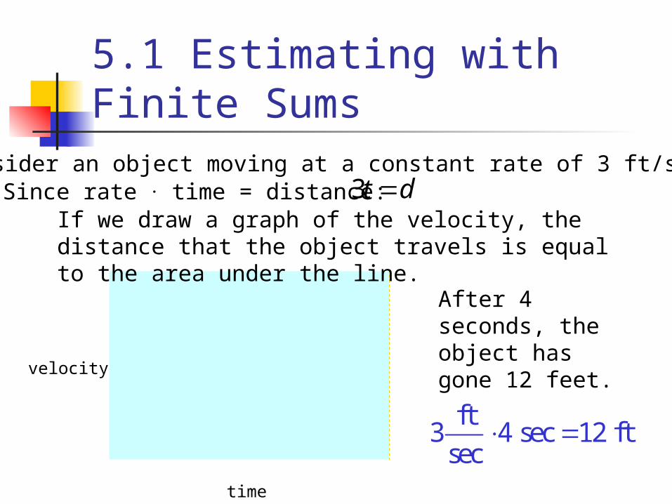
time
velocity
After 4 seconds, the object has gone 12 feet.
Consider an object moving at a constant rate of 3 ft/sec.Since rate . time = distance:If we draw a graph of the velocity, the distance that the object travels is equal to the area under the line.
ft3 4 sec 12 ft
sec
3t d
5.1 Estimating with Finite Sums
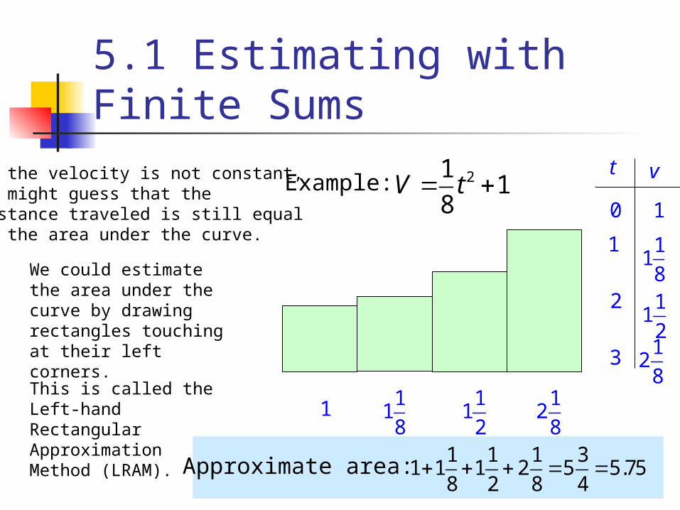
If the velocity is not constant,we might guess that the distance traveled is still equalto the area under the curve.
211
8V t Example:
We could estimate the area under the curve by drawing rectangles touching at their left corners.
This is called the Left-hand Rectangular Approximation Method (LRAM).
1 11
8
11
2
12
8
t v
10
1 11
82 1
12
3 12
8
Approximate area: 1 1 1 31 1 1 2 5 5.75
8 2 8 4
5.1 Estimating with Finite Sums
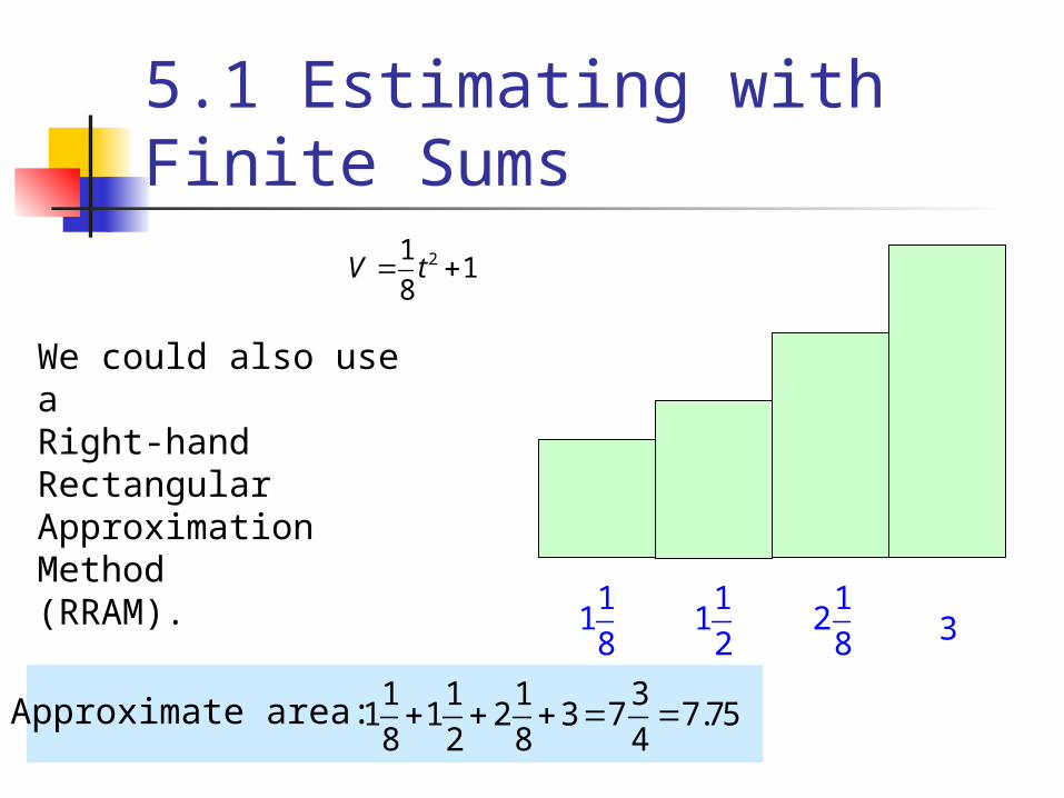
We could also use a Right-hand Rectangular Approximation Method(RRAM).
11
8
11
2
12
8
Approximate area: 1 1 1 31 1 2 3 7 7.75
8 2 8 4
3
211
8V t
5.1 Estimating with Finite Sums
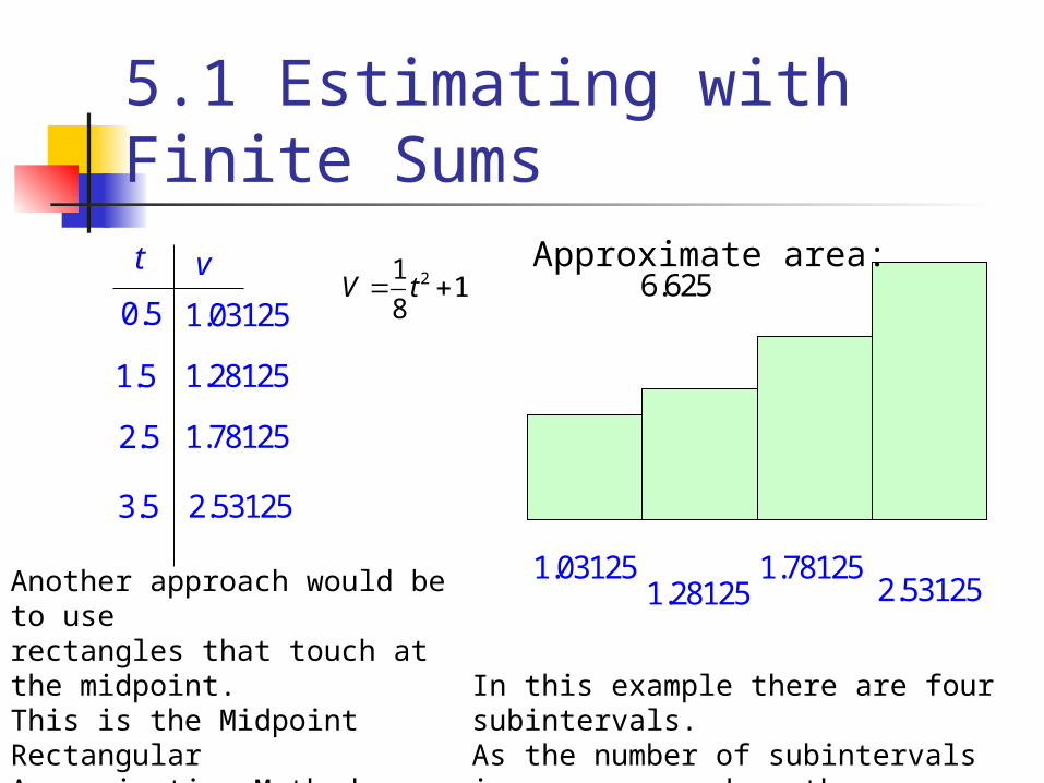
Another approach would be to userectangles that touch at the midpoint. This is the Midpoint Rectangular Approximation Method (MRAM).
1.031251.28125
1.78125
Approximate area:6.625
2.53125
t v
1.031250.5
1.5 1.28125
2.5 1.78125
3.5 2.53125
In this example there are four subintervals.As the number of subintervals increases, so does the accuracy.
211
8V t
5.1 Estimating with Finite Sums
211
8V t
Approximate area:6.65624
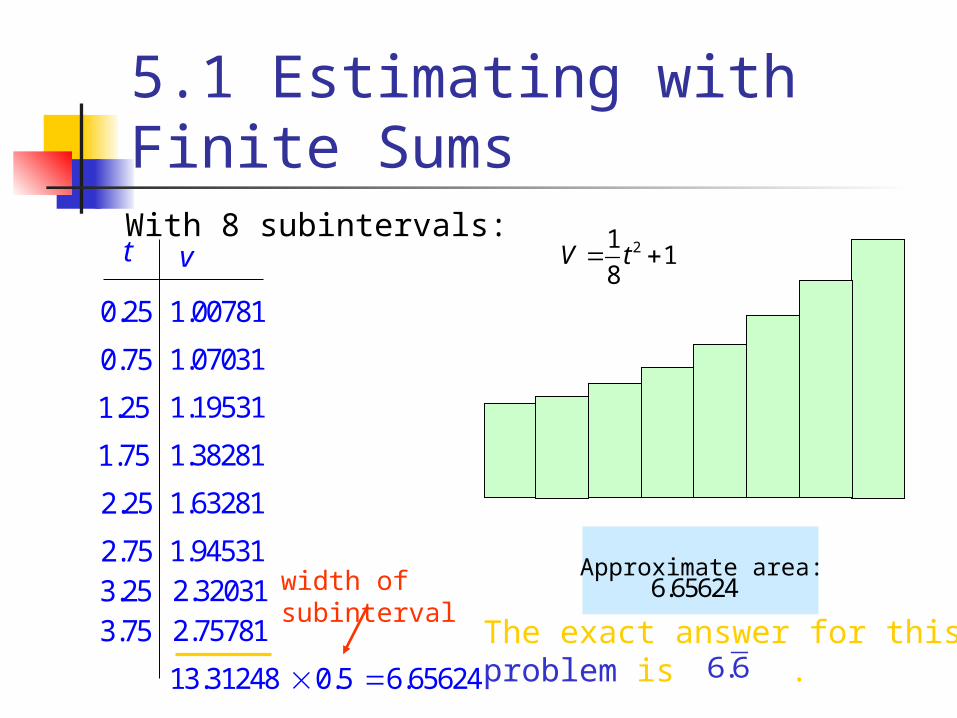
t v
1.007810.25
0.75 1.07031
1.25 1.19531
1.382811.75
2.25
2.753.253.75
1.63281
1.945312.320312.75781
13.31248 0.5 6.65624
width of subinterval
With 8 subintervals:
The exact answer for thisproblem is .6.6
5.1 Estimating with Finite Sums
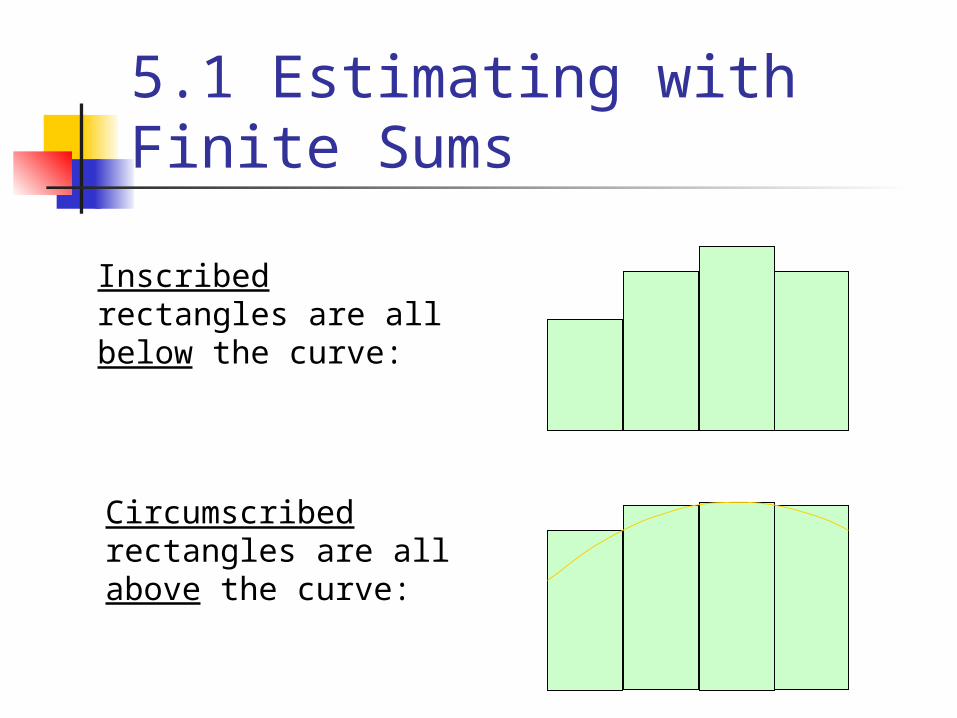
Circumscribed rectangles are all above the curve:
Inscribed rectangles are all below the curve:
5.1 Estimating with Finite Sums
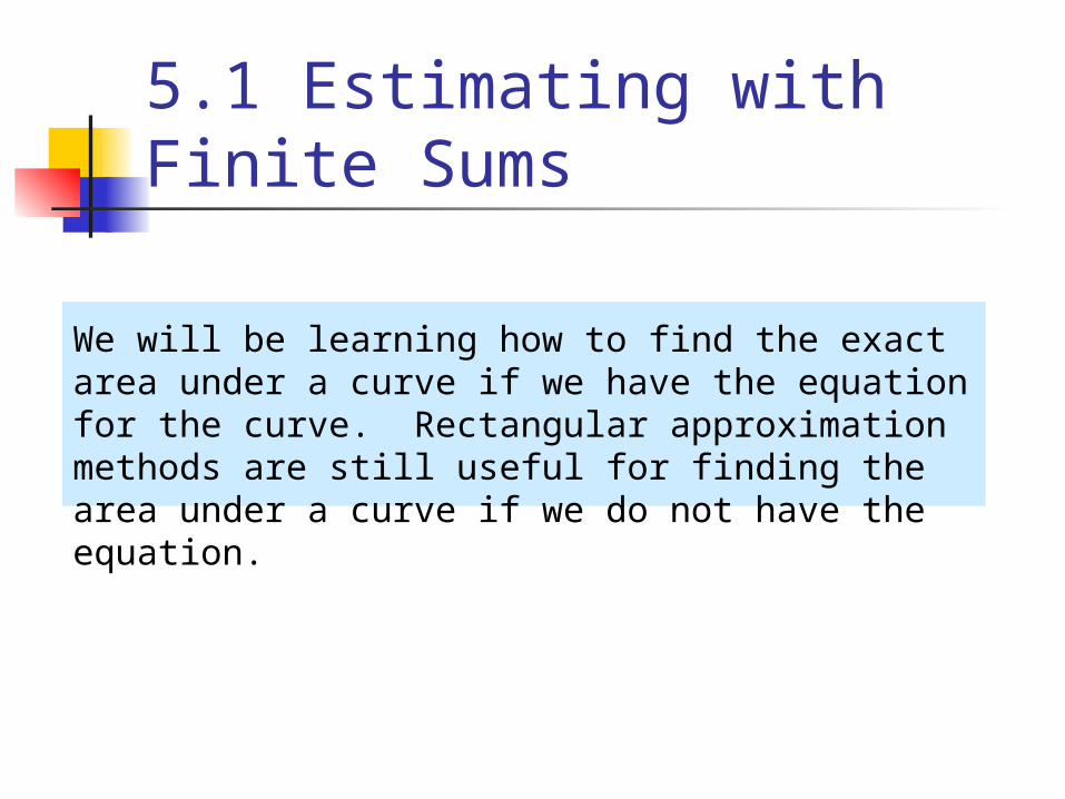
We will be learning how to find the exact area under a curve if we have the equation for the curve. Rectangular approximation methods are still useful for finding the area under a curve if we do not have the equation.
5.1 Estimating with Finite Sums
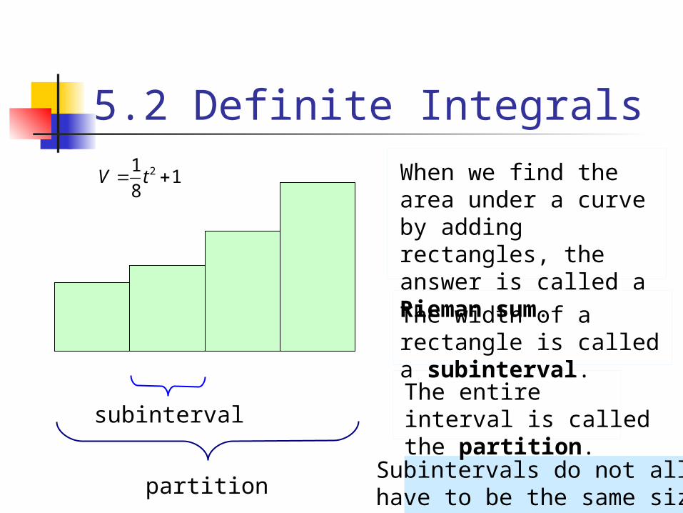
When we find the area under a curve by adding rectangles, the answer is called a Rieman sum.
211
8V t
subinterval
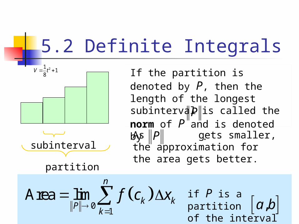
partition
The width of a rectangle is called a subinterval.
The entire interval is called the partition.
Subintervals do not all have to be the same size.
5.2 Definite Integrals
211
8V t
subinterval
partition
If the partition is denoted by P, then the length of the longest subinterval is called the norm of P and is denoted by .P
As gets smaller, the approximation for the area gets better.
P
0
1
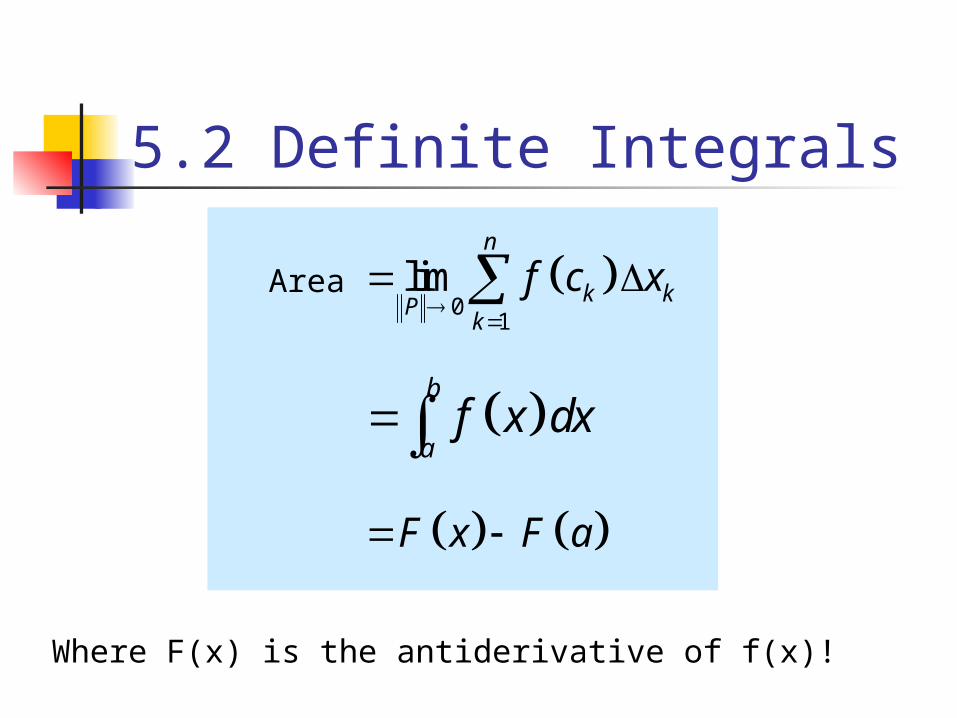
Area limn
k kP
k
f c x
if P is a partition of the interval ,a b
5.2 Definite Integrals
0
1
limn
k kP
k
f c x
is called the definite integral of
over .f ,a b
If we use subintervals of equal length, then the length of a
subinterval is:b a
xn
The definite integral is then given by: 1
limn
kn
k
f c x
5.2 Definite Integrals
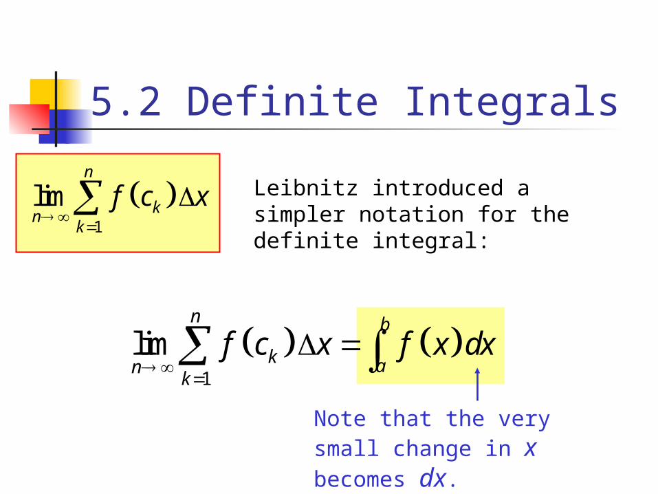
1
limn
kn
k
f c x
Leibnitz introduced a simpler notation for the definite integral:
1
limn b
k ank
f c x f x dx
Note that the very small change in x becomes dx.
5.2 Definite Integrals
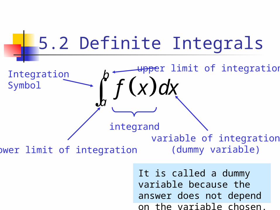
b
af x dx
IntegrationSymbol
lower limit of integration
upper limit of integration
integrandvariable of integration
(dummy variable)
It is called a dummy variable because the answer does not depend on the variable chosen.
5.2 Definite Integrals
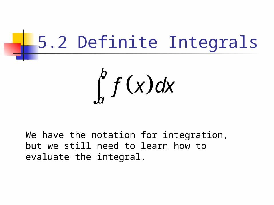
b
af x dx
We have the notation for integration, but we still need to learn how to evaluate the integral.
5.2 Definite Integrals
5.2 Definite Integrals
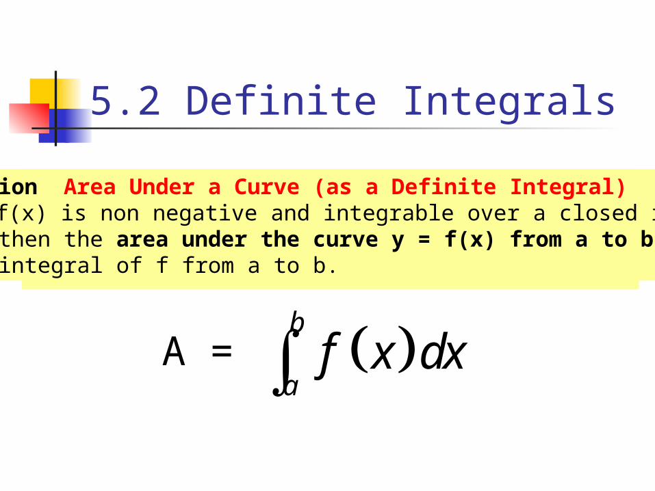
Definition Area Under a Curve (as a Definite Integral)If y = f(x) is non negative and integrable over a closed interval[a,b], then the area under the curve y = f(x) from a to b is the integral of f from a to b.
b
af x dxA =
time
velocity
After 4 seconds, the object has gone 12 feet.
In section 5.1, we considered an object moving at a constant rate of 3 ft/sec.
3t d
If we draw a graph of the velocity, the distance that the object travels is equal to the area under the line.
ft3 4 sec 12 ft
sec
5.2 Definite Integrals
If the velocity varies:
11
2v t
Distance is the area under the curve
8s
5.2 Definite Integrals
)bh(b2
1A 21trapezoid
3)4(12
1Atrapezoid
0
1
limn
k kP
k
f c x
b
af x dx
F x F a
Area
Where F(x) is the antiderivative of f(x)!
5.2 Definite Integrals
211
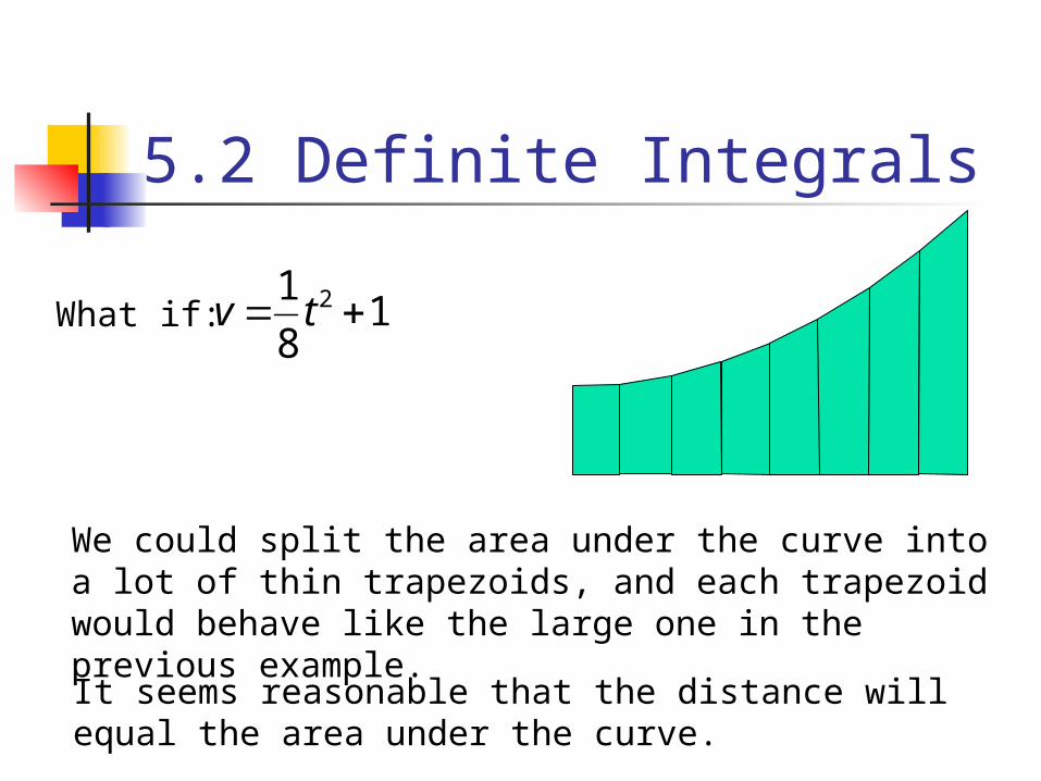
8v t What if:
We could split the area under the curve into a lot of thin trapezoids, and each trapezoid would behave like the large one in the previous example.
It seems reasonable that the distance will equal the area under the curve.
5.2 Definite Integrals
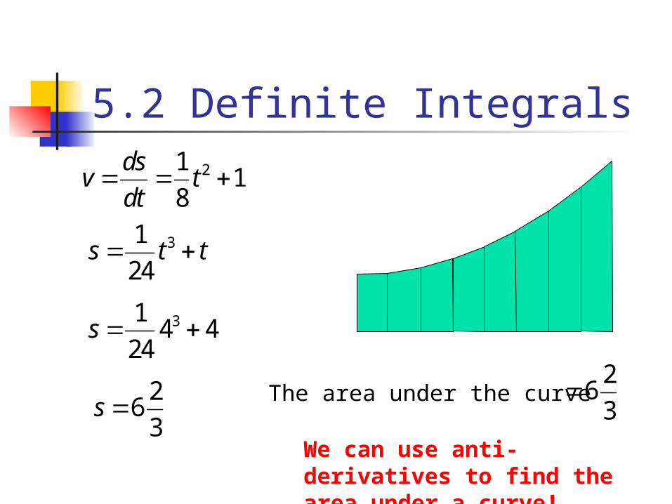
211
8
dsv t
dt
31
24s t t
314 4
24s
26
3s The area under the curve
26
3
We can use anti-derivatives to find the area under a curve!
5.2 Definite Integrals
Area from x=0to x=1
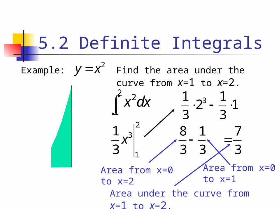
Example:2y x Find the area under the curve from
x=1 to x=2.2 2
1x dx
23
1
1
3x
31 12 1
3 3
8 1
3 3
7
3
Area from x=0to x=2
Area under the curve from x=1 to x=2.
5.2 Definite Integrals
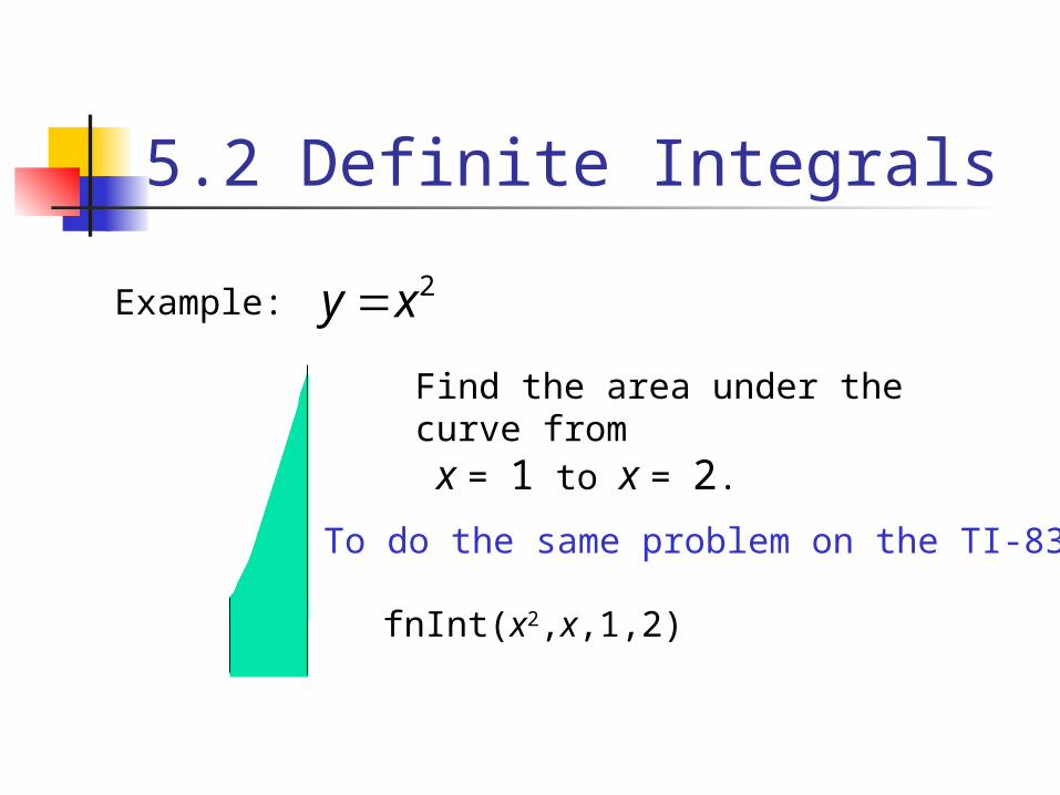
Example: 2y x
Find the area under the curve from x = 1 to x = 2.
To do the same problem on the TI-83:
fnInt(x2,x,1,2)
5.2 Definite Integrals
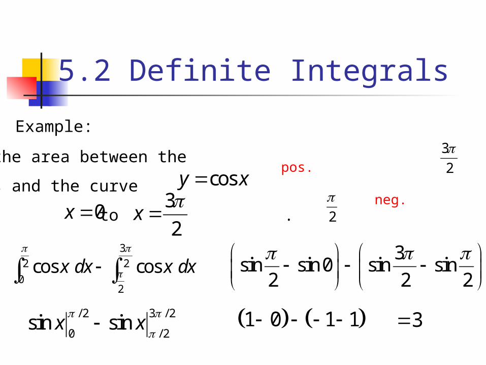
Example:
Find the area between the
x-axis and the curve
from to .
cosy x
0x 3
2x
2
3
2
3
2 2
02
cos cos x dx x dx
/ 2 3 / 2
0 / 2sin sinx x
3sin sin 0 sin sin
2 2 2
1 0 1 1 3
pos.
neg.
5.2 Definite Integrals
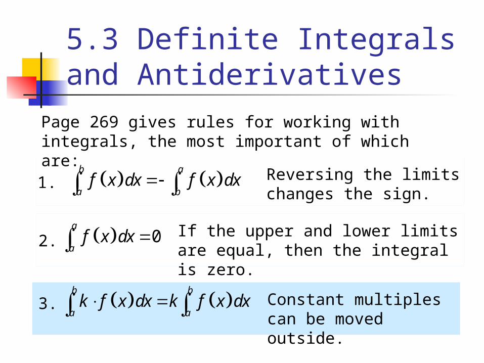
Page 269 gives rules for working with integrals, the most important of which are:
2. 0a
af x dx If the upper and lower limits are equal,
then the integral is zero.
1. b a
a bf x dx f x dx Reversing the limits
changes the sign.
b b
a ak f x dx k f x dx 3. Constant multiples can be
moved outside.
5.3 Definite Integrals and Antiderivatives
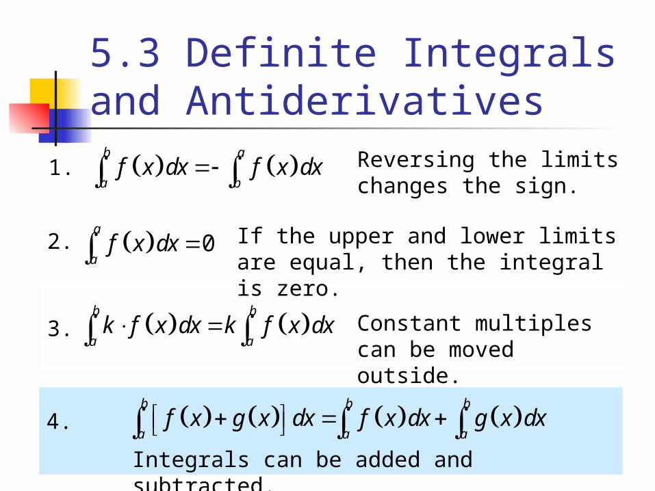
1.
0a
af x dx If the upper and lower limits are equal,
then the integral is zero.2.
b a
a bf x dx f x dx Reversing the limits
changes the sign.
b b
a ak f x dx k f x dx 3. Constant multiples can be
moved outside.
b b b
a a af x g x dx f x dx g x dx 4.
Integrals can be added and subtracted.
5.3 Definite Integrals and Antiderivatives
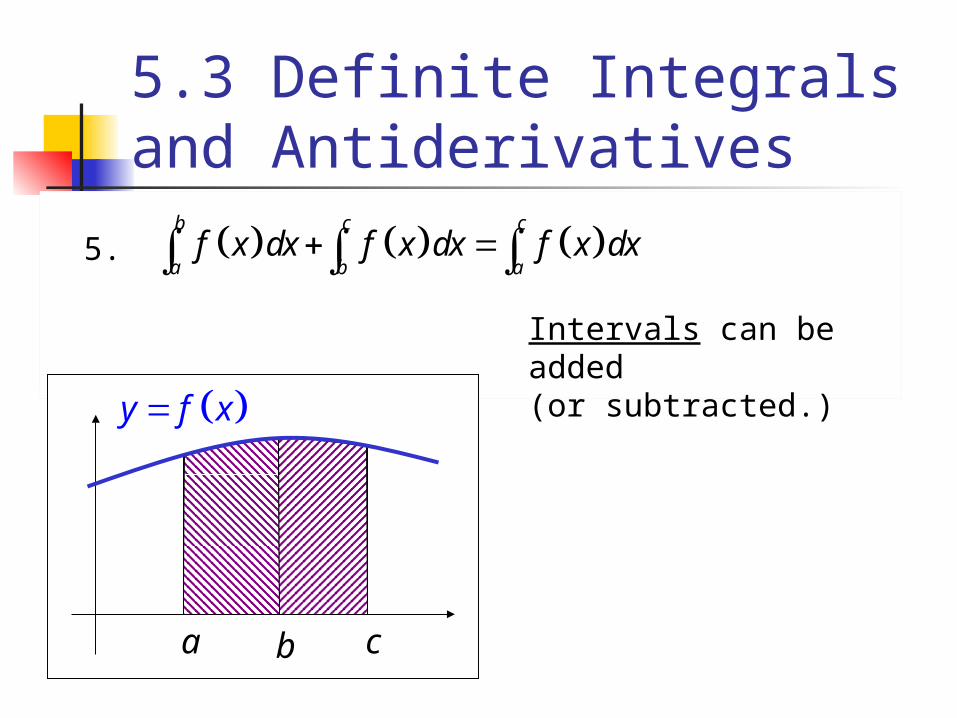
5. b c c
a b af x dx f x dx f x dx
Intervals can be added(or subtracted.)
a b c
y f x
5.3 Definite Integrals and Antiderivatives
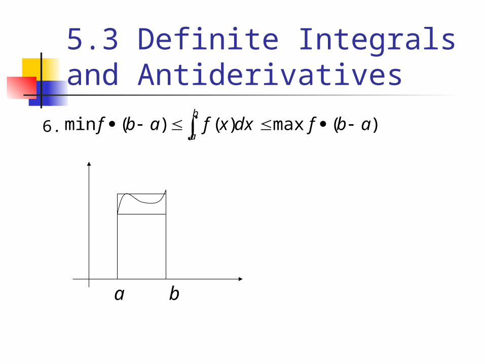
6.
5.3 Definite Integrals and Antiderivatives
b
aabfdxxfabf )(max)()(min
a b
5.3 Definite Integrals and Antiderivatives
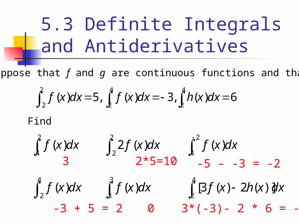
Suppose that f and g are continuous functions and that
4
2
2
2
4
26)(,3)(,5)( dxxhdxxfdxxf
Find
2
4)( dxxf
4
2)( dxxf
2
2)(2 dxxf
3
3)( dxxf
2
4)( dxxf
4
2)](2)(3[ dxxhxf
3 2*5=10 -5 – -3 = -2
-3 + 5 = 2 0 3*(-3)- 2 * 6 = -21
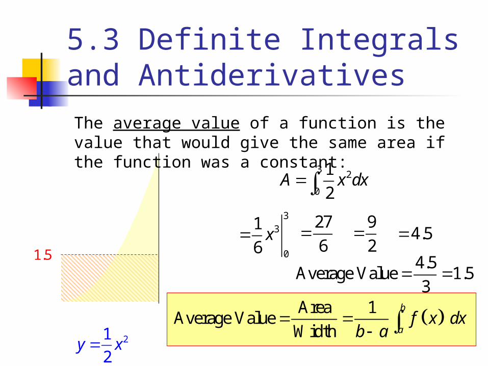
The average value of a function is the value that would give the same area if the function was a constant:
21
2y x
3 2
0
1
2A x dx3
3
0
1
6x
27
6
9
2 4.5
4.5Average Value 1.5
3
Area 1Average Value
Width
b
af x dx
b a
1.5
5.3 Definite Integrals and Antiderivatives
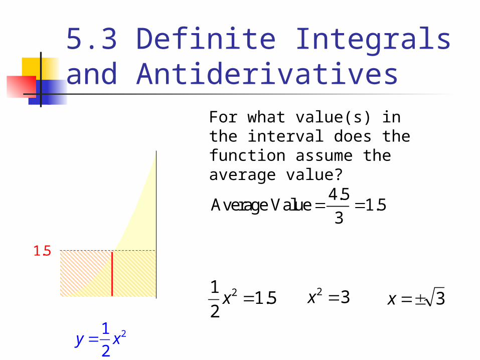
For what value(s) in the interval does the function assume the average value?
21
2y x
4.5Average Value 1.5
3
1.5
5.3 Definite Integrals and Antiderivatives
5.12
1 2 x 32 x 3x
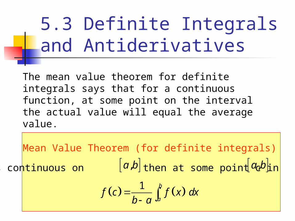
The mean value theorem for definite integrals says that for a continuous function, at some point on the interval the actual value will equal the average value.
Mean Value Theorem (for definite integrals)
If f is continuous on then at some point c in , ,a b ,a b
1
b
af c f x dx
b a
5.3 Definite Integrals and Antiderivatives
5.3 Definite Integrals and Antiderivatives
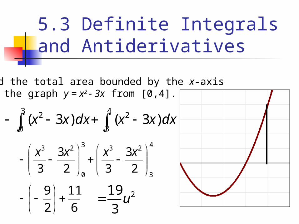
Find the total area bounded by the x-axisand the graph y = x2 - 3x from [0,4].
dxxxdxxx 4
3
23
0
2 )3()3(
4
3
233
0
23
2
3
32
3
3
xxxx
6
11
2
9
2
3
19u
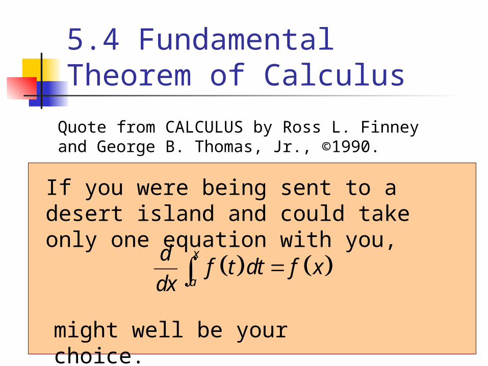
If you were being sent to a desert island and could take only one equation with you,
x
a
df t dt f x
dx
might well be your choice.
Quote from CALCULUS by Ross L. Finney and George B. Thomas, Jr., ©1990.
5.4 Fundamental Theorem of Calculus
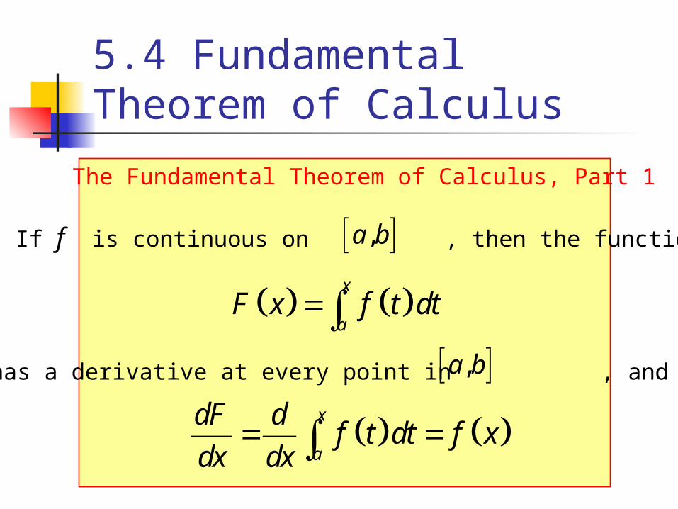
The Fundamental Theorem of Calculus, Part 1
If f is continuous on , then the function ,a b
x
aF x f t dt
has a derivative at every point in , and ,a b
x
a
dF df t dt f x
dx dx
5.4 Fundamental Theorem of Calculus
x
a
df t dt f x
dx
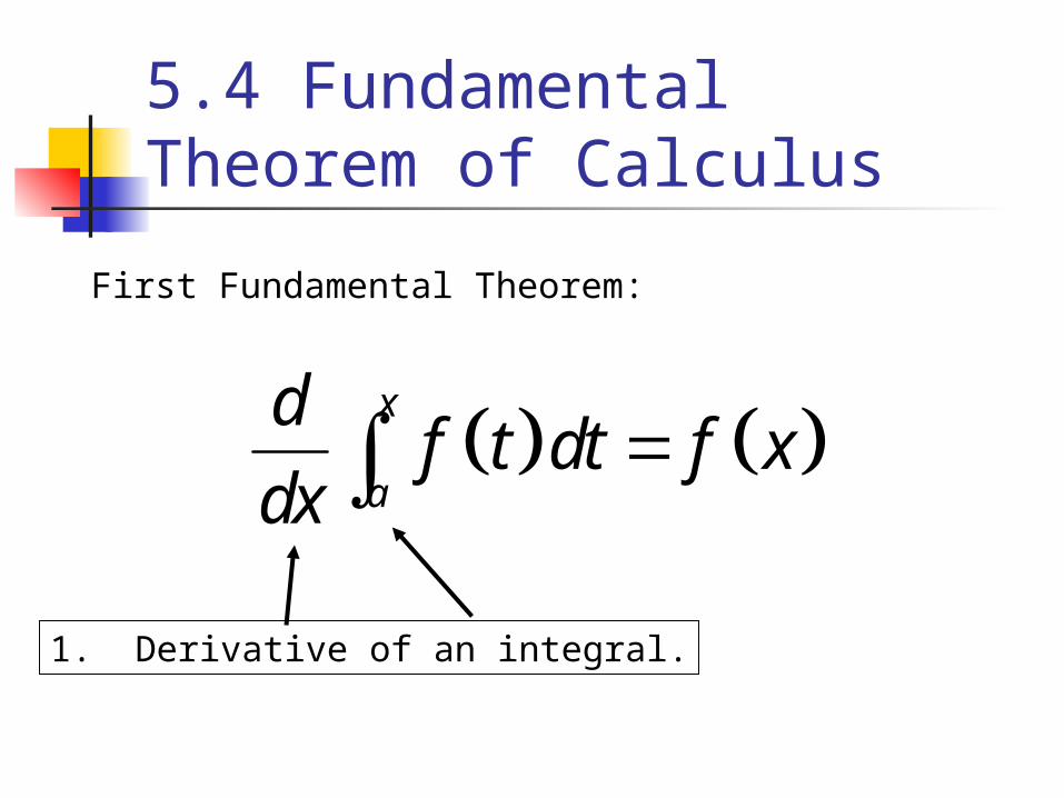
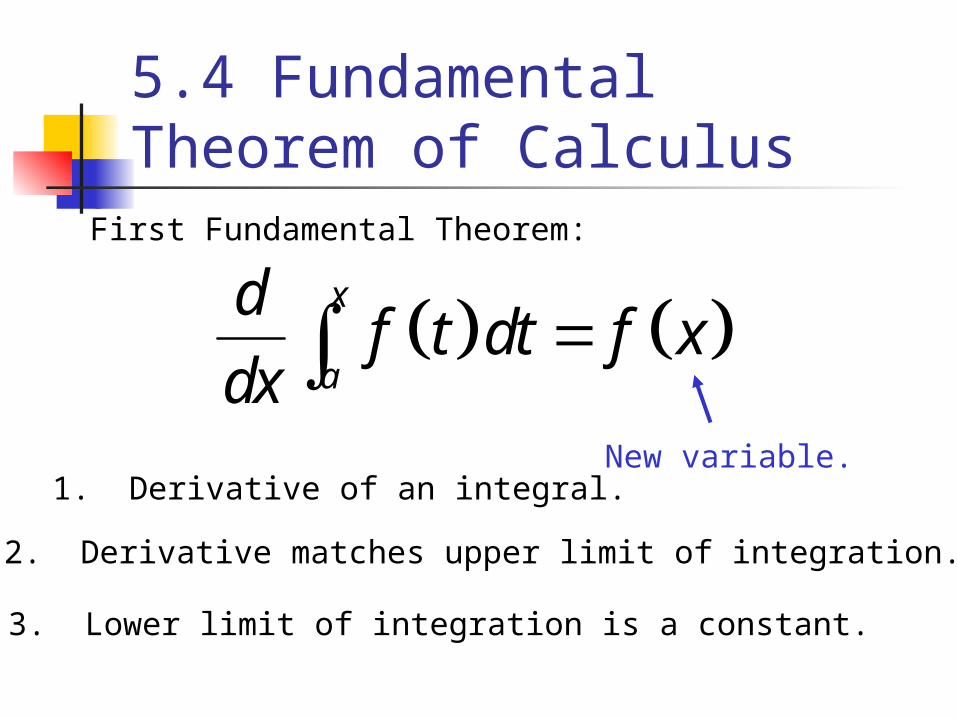
First Fundamental Theorem:
1. Derivative of an integral.
5.4 Fundamental Theorem of Calculus
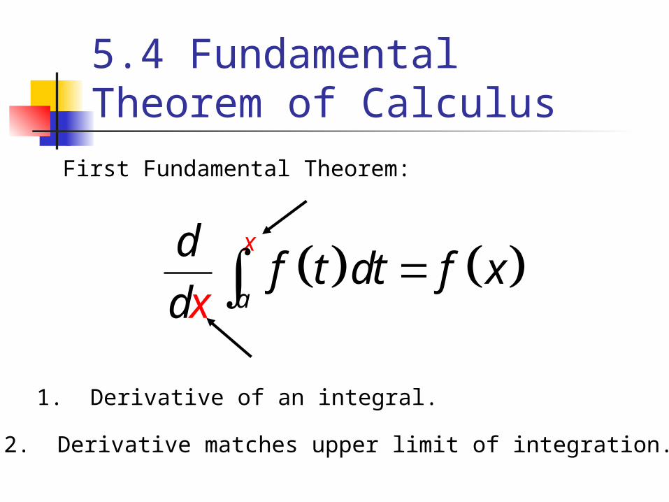
a
xdf t dt
xf x
d
2. Derivative matches upper limit of integration.
First Fundamental Theorem:
1. Derivative of an integral.
5.4 Fundamental Theorem of Calculus
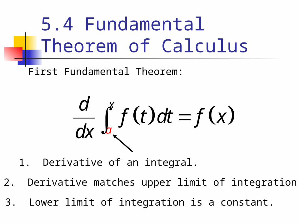
a
xdf t dt f x
dx
1. Derivative of an integral.
2. Derivative matches upper limit of integration.
3. Lower limit of integration is a constant.
First Fundamental Theorem:
5.4 Fundamental Theorem of Calculus
x
a
df t dt f x
dx
1. Derivative of an integral.
2. Derivative matches upper limit of integration.
3. Lower limit of integration is a constant.
New variable.
First Fundamental Theorem:
5.4 Fundamental Theorem of Calculus
cos xd
t dtdx cos x
1. Derivative of an integral.
2. Derivative matches upper limit of integration.
3. Lower limit of integration is a constant.
sinxd
tdx
sin sind
xdx
0
sind
xdx
The long way:First Fundamental Theorem:
5.4 Fundamental Theorem of Calculus
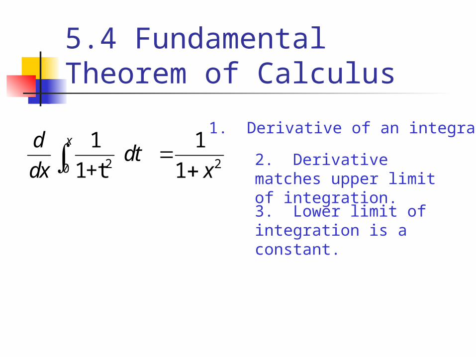
20
1
1+t
xddt
dx 2
1
1 x
1. Derivative of an integral.
2. Derivative matches upper limit of integration.
3. Lower limit of integration is a constant.
5.4 Fundamental Theorem of Calculus
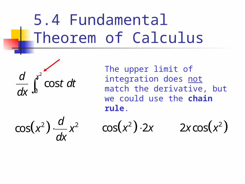
2
0cos
xdt dt
dx
2 2cosd
x xdx
2cos 2x x 22 cosx x
The upper limit of integration does not match the derivative, but we could use the chain rule.
5.4 Fundamental Theorem of Calculus
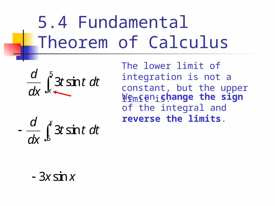
53 sin
x
dt t dt
dx The lower limit of integration is not a constant, but the upper limit is.
53 sin
xdt t dt
dx
3 sinx x
We can change the sign of the integral and reverse the limits.
5.4 Fundamental Theorem of Calculus
2
2
1
2
x
tx
ddt
dx eNeither limit of integration is a constant.
2 0
0 2
1 1
2 2
x
t tx
ddt dt
dx e e
It does not matter what constant we use!
2 2
0 0
1 1
2 2
x x
t t
ddt dt
dx e e
2 2
1 12 2
22xx
xee
(Limits are reversed.)
(Chain rule is used.)
2 2
2 2
22xx
x
ee
We split the integral into two parts.
5.4 Fundamental Theorem of Calculus
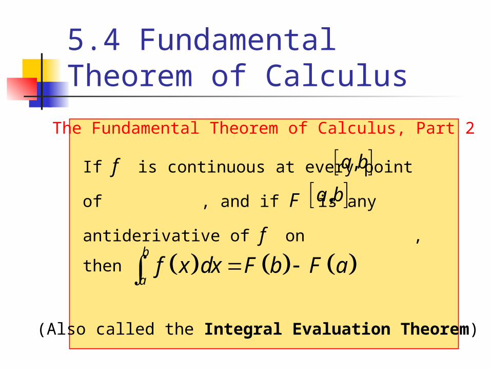
The Fundamental Theorem of Calculus, Part 2
If f is continuous at every point of , and if
F is any antiderivative of f on , then
,a b
b
af x dx F b F a
,a b
(Also called the Integral Evaluation Theorem)
5.4 Fundamental Theorem of Calculus
5.4 Fundamental Theorem of Calculus
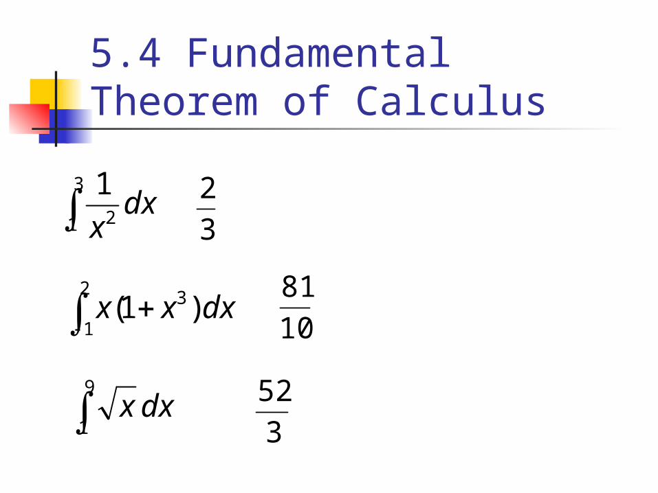
dxx
3
1 2
1
3
2
dxxx 2
1
3)1(10
81
dxx9
1 3
52
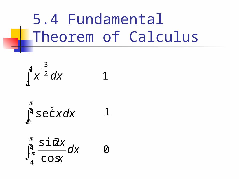
5.4 Fundamental Theorem of Calculus
dxx4
1
2
3
1
dxx4
0
2sec
1
dxx
x4
4 cos
2sin
0
5.4 Fundamental Theorem of Calculus
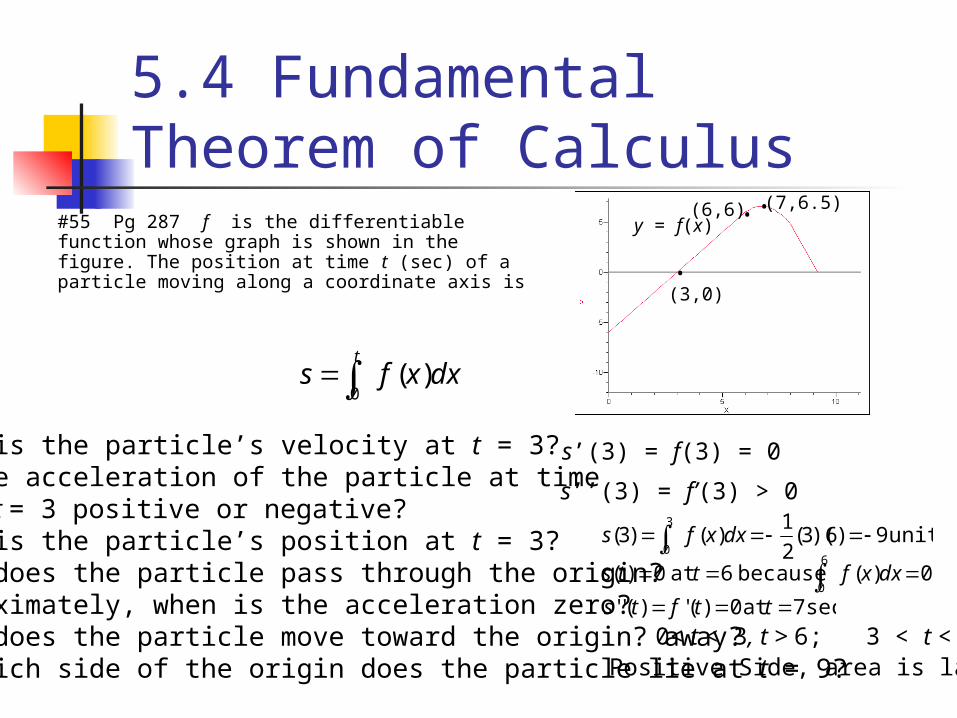
#55 Pg 287 f is the differentiable function whose graph is shown in the figure. The position at time t (sec) of a particle moving along a coordinate axis is
t
dxxfs0
)(
a. What is the particle’s velocity at t = 3?b. Is the acceleration of the particle at time t = 3 positive or negative?c. What is the particle’s position at t = 3?d. When does the particle pass through the origin?e. Approximately, when is the acceleration zero?f. When does the particle move toward the origin? away?g. On which side of the origin does the particle lie at t = 9?
(3,0)
y = f(x)(6,6) (7,6.5)
•
•
•
s’(3) = f(3) = 0
s’’(3) = f’(3) > 0
units9)6)(3(2
1)()3(
3
0 dxxfs
6
00)(because6at0)( dxxftts
sec7at0)(')('' ttfts
0< t < 3, t > 6; 3 < t < 6Positive Side, area is larger
Using integrals to find area works extremely well as long as we can find the antiderivative of the function.
Sometimes, the function is too complicated to find the antiderivative.
At other times, we don’t even have a function, but only measurements taken from a real-life object.
What we need is an efficient method to estimate area when we can not find the antiderivative.
5.5 Trapezoid Rule
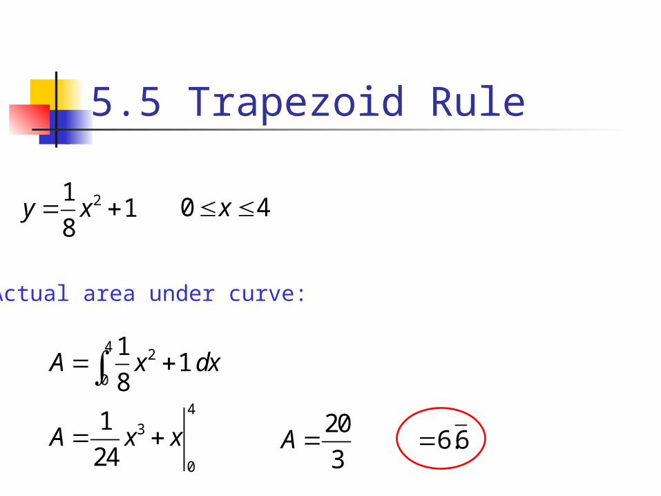
211
8y x
43
0
1
24A x x
4 2
0
11
8A x dx
0 4x
Actual area under curve:
20
3A 6.6
5.5 Trapezoid Rule
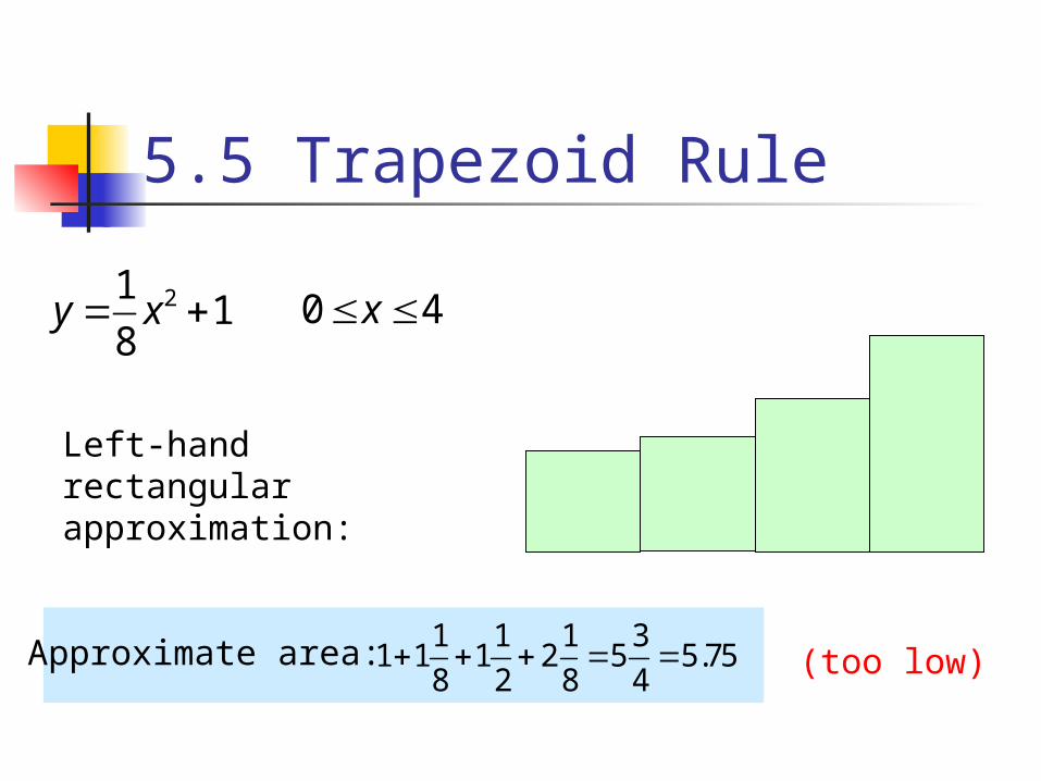
211
8y x 0 4x
Left-hand rectangular approximation:
Approximate area: 1 1 1 31 1 1 2 5 5.75
8 2 8 4 (too low)
5.5 Trapezoid Rule
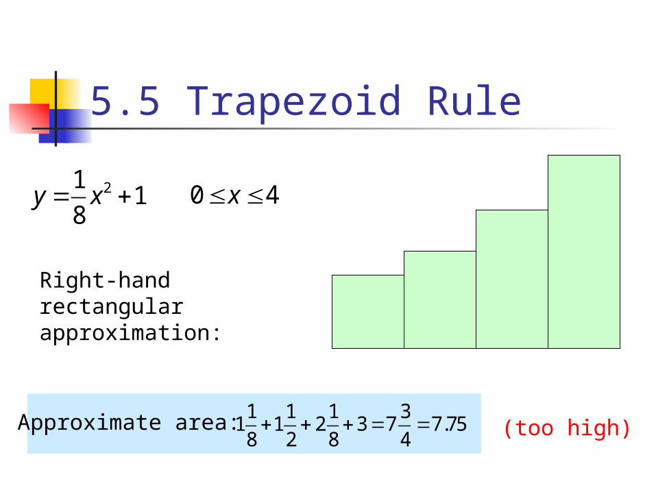
Approximate area: 1 1 1 31 1 2 3 7 7.75
8 2 8 4
211
8y x 0 4x
Right-hand rectangular approximation:
(too high)
5.5 Trapezoid Rule
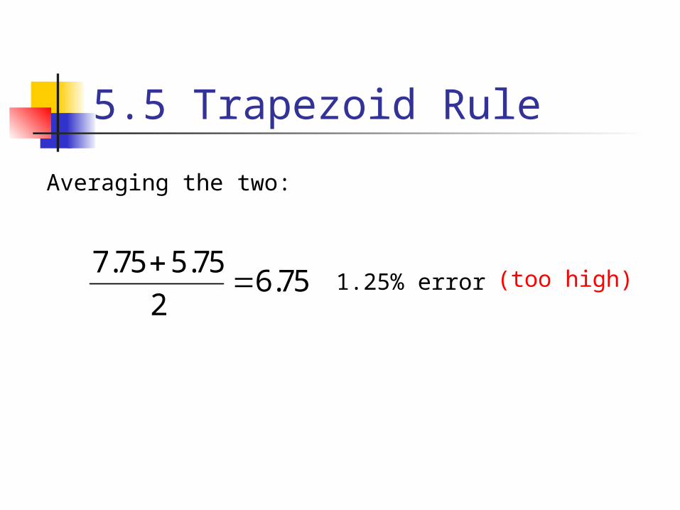
Averaging the two:
7.75 5.756.75
2
1.25% error (too high)
5.5 Trapezoid Rule
5.5 Trapezoid Rule
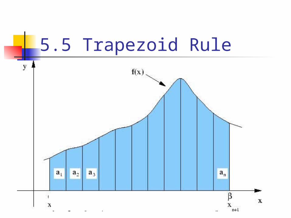
xo=a x1 x2 x3 xn-1 xn = b
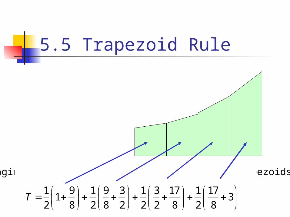
Averaging right and left rectangles gives us trapezoids:
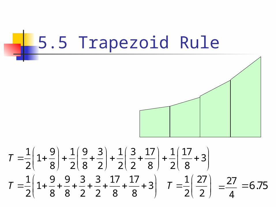
1 9 1 9 3 1 3 17 1 171 3
2 8 2 8 2 2 2 8 2 8T
5.5 Trapezoid Rule
1 9 1 9 3 1 3 17 1 171 3
2 8 2 8 2 2 2 8 2 8T
1 9 9 3 3 17 171 3
2 8 8 2 2 8 8T
1 27
2 2T
27
4 6.75
5.5 Trapezoid Rule
5.5 Trapezoid Rule
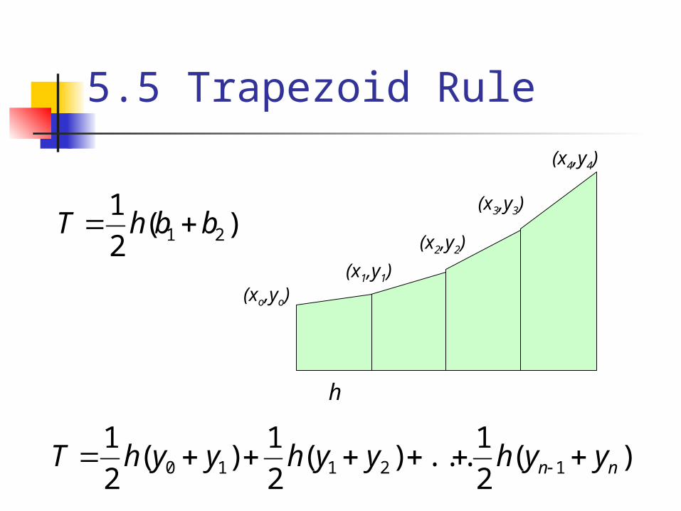
)(2
121 bbhT
(xo,yo)(x1,y1)
(x2,y2)
(x3,y3)
(x4,y4)
h
)(2
1...)(
2
1)(
2
112110 nn yyhyyhyyhT
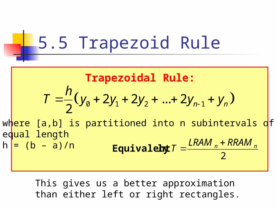
Trapezoidal Rule:
0 1 2 12 2 ... 22 n n
hT y y y y y
where [a,b] is partitioned into n subintervals ofequal lengthh = (b – a)/n
This gives us a better approximation than either left or right rectangles.
5.5 Trapezoid Rule
2nn RRAMLRAM
T
lyEquivalent
5.5 Trapezoid Rule
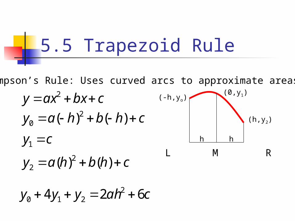
Simpson’s Rule: Uses curved arcs to approximate areas
cbxaxy 2 (-h,yo)(0,y1)
(h,y2)chbhay )()( 20
L M R
h hcy 1
chbhay )()( 22
cahyyy 624 2210
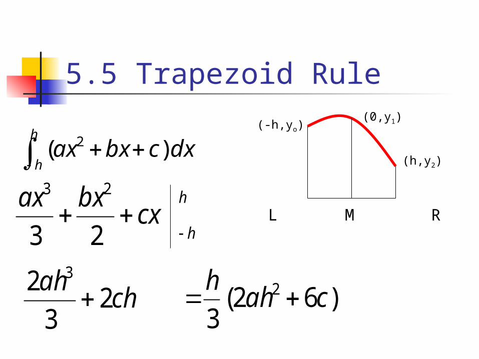
5.5 Trapezoid Rule
dxcbxaxh
h)( 2
(-h,yo)(0,y1)
(h,y2)
L M Rh
hcx
bxax
23
23
chah
23
2 3
)62(3
2 cahh
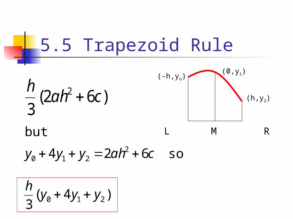
5.5 Trapezoid Rule
(-h,yo)(0,y1)
(h,y2)
L M R
)62(3
2 cahh
)4(3 210 yyyh
but
cahyyy 624 2210 so
Simpson’s Rule:
5.5 Trapezoid Rule
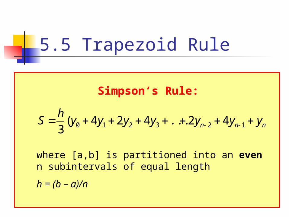
nnn yyyyyyyh
S 123210 42...424(3
where [a,b] is partitioned into an even n subintervals of equal length
h = (b – a)/n
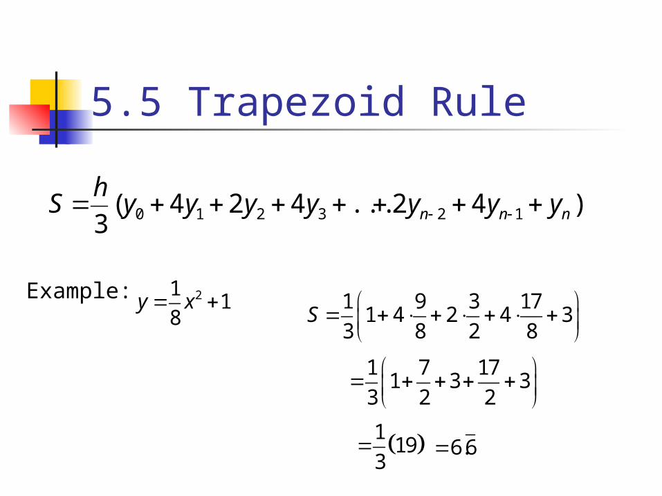
Example: 211
8y x 1 9 3 17
1 4 2 4 33 8 2 8
S
1 7 171 3 3
3 2 2
119
3 6.6
5.5 Trapezoid Rule
)42...424(3 123210 nnn yyyyyyyh
S
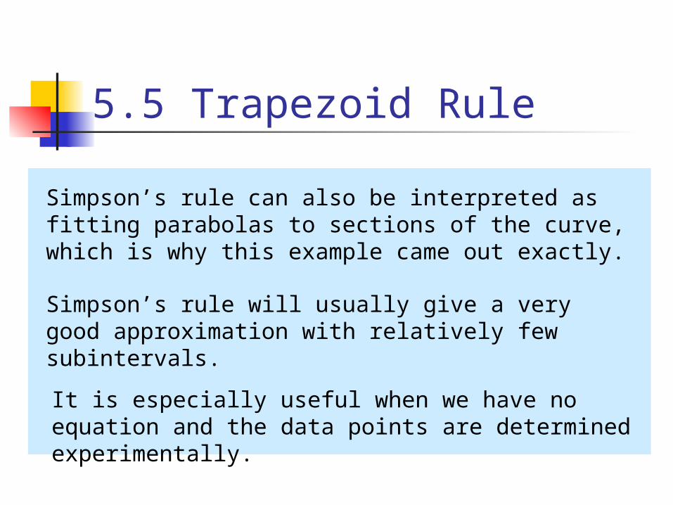
Simpson’s rule can also be interpreted as fitting parabolas to sections of the curve, which is why this example came out exactly.
Simpson’s rule will usually give a very good approximation with relatively few subintervals.
It is especially useful when we have no equation and the data points are determined experimentally.
5.5 Trapezoid Rule
5.5 Trapezoid Rule
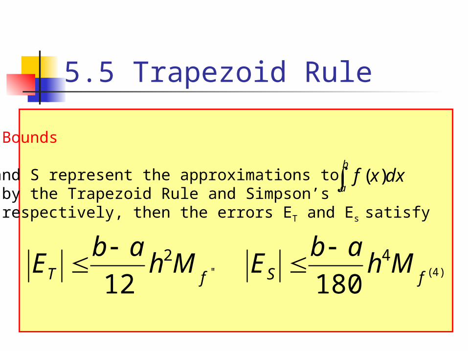
Error Bounds
If T and S represent the approximations togiven by the Trapezoid Rule and Simpson’s Rule, respectively, then the errors ET and Es satisfy
b
adxxf )(
''2
12 fT Mhab
E
)4(4
180 fS Mhab
E