Embed Size (px)
Citation preview

14
Image Acquisition Rate Control Based on Object State Information in Physical
and Image Coordinates
Feng-Li Lian and Shih-Yuan Peng Department of Electrical Engineering, National Taiwan University
Taipei, Taiwan
1. Introduction
Recently, three-dimensional (3-D) vision applications play an important role in industry and
entertainment. Among these applications, interactivity and scene reality are the two key
features affecting the 3-D vision performance. Depending on the nature of the applications,
the interactivity with the users (or the players) can be regarded as an important need, for
example, in the applications of 3-D games and 3-D virtual reality. On the other hand, 3-D
vision scenes can be generated based on physical or virtual models. In order to improve the
scene reality, a new trend in 3-D vision system is to generate the scene based on some
physical or real-world models.
For the 3-D reconstruction, research topics mainly focus on the static cases and/ or the
dynamic cases. For the static cases, the reconstructed scenes do not change with the
observed scenes. For the dynamic cases, the reconstructed scenes change with the observed
scenes. For both static and dynamic cases, the 3-D positioning of moving objects in the scene
is the major component of obtaining the object states in the physical coordinate. A typical 3-
D positioning system is shown in Figure 1. Cameras shown in Figure 1 are used to capture
the images of moving objects in the physical coordinate. The image acquisition rate of
Camera X is denoted as Rate X. After one camera captures the images using its designated
acquisition rate, the captured images are stored and analyzed in the computer. After
analyzing the images, the object states, e.g., position and velocity, in the physical coordinate
can be estimated by any 3-D positioning method.
The 3-D positioning plays an important role of obtaining the object states in the physical
coordinate. In general, cameras are designated as the input devices for capturing images.
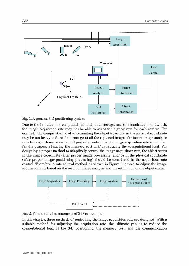
Fundamental components of 3-D positioning are shown in Figure 2. First of all, images are
captured by the input devices such as cameras. Before the image acquisition, the camera
calibration should be done. Based on the calibration result, the relationship between the
physical coordinate and the image coordinate in the captured images can be obtained. Since
the quality of the captured images may be influenced by noise, some image processes
should be performed to eliminate the noise. After the image processing, the captured images
can be analyzed to extract the object information for further 3-D positioning. Finally, any 3-
D positioning method is used to find the object states such as the position and/ or velocity in
the physical coordinate. Ope
n A
cces
s D
atab
ase
ww
w.i-
tech
onlin
e.co
m
Source: Computer Vision, Book edited by: Xiong Zhihui, ISBN 978-953-7619-21-3, pp. 538, November 2008, I-Tech, Vienna, Austria
www.intechopen.com
Computer Vision
232
Object
3-D Space
Object
3-D Space
Rate B
B A
Rate A
Image
Acquisition
Image
Analysis
3-D
Positioning
Image
Information
Object
Information
Rate
Control
Computer
Physical Domain
Object
3-D Space
Object
3-D Space
Rate B
B A
Rate A
Image
Acquisition
Image
Analysis
3-D
Positioning
Image
Information
Object
Information
Rate
Control
Computer
Physical Domain
Fig. 1. A general 3-D positioning system
Due to the limitation on computational load, data storage, and communication bandwidth,
the image acquisition rate may not be able to set at the highest rate for each camera. For
example, the computation load of estimating the object trajectory in the physical coordinate
may be too heavy and the data storage of all the captured images for future image analysis
may be huge. Hence, a method of properly controlling the image acquisition rate is required
for the purpose of saving the memory cost and/ or reducing the computational load. For
designing a proper method to adaptively control the image acquisition rate, the object states
in the image coordinate (after proper image processing) and/ or in the physical coordinate
(after proper image/ positioning processing) should be considered in the acquisition rate
control. Therefore, a rate control method as shown in Figure 2 is used to adjust the image
acquisition rate based on the result of image analysis and the estimation of the object states.
Image Acquisition Image Processing Image AnalysisEstimation of
3-D object location
Rate Control
Fig. 2. Fundamental components of 3-D positioning
In this chapter, three methods of controlling the image acquisition rate are designed. With a
suitable method for adjusting the acquisition rate, the ultimate goal is to reduce the
computational load of the 3-D positioning, the memory cost, and the communication
www.intechopen.com
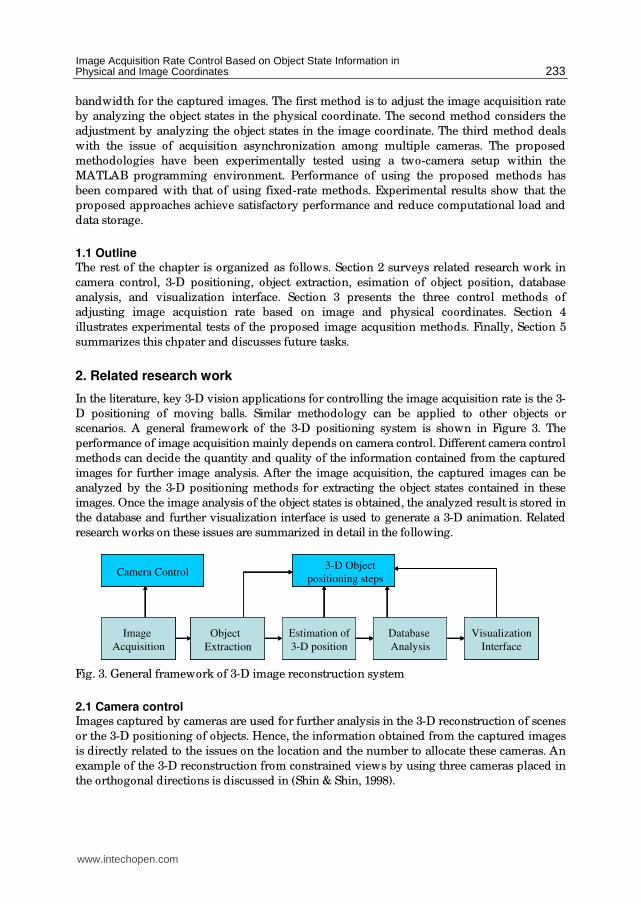
Image Acquisition Rate Control Based on Object State Information in Physical and Image Coordinates
233
bandwidth for the captured images. The first method is to adjust the image acquisition rate
by analyzing the object states in the physical coordinate. The second method considers the
adjustment by analyzing the object states in the image coordinate. The third method deals
with the issue of acquisition asynchronization among multiple cameras. The proposed
methodologies have been experimentally tested using a two-camera setup within the
MATLAB programming environment. Performance of using the proposed methods has
been compared with that of using fixed-rate methods. Experimental results show that the
proposed approaches achieve satisfactory performance and reduce computational load and
data storage.
1.1 Outline The rest of the chapter is organized as follows. Section 2 surveys related research work in
camera control, 3-D positioning, object extraction, esimation of object position, database
analysis, and visualization interface. Section 3 presents the three control methods of
adjusting image acquistion rate based on image and physical coordinates. Section 4
illustrates experimental tests of the proposed image acqusition methods. Finally, Section 5
summarizes this chpater and discusses future tasks.
2. Related research work
In the literature, key 3-D vision applications for controlling the image acquisition rate is the 3-
D positioning of moving balls. Similar methodology can be applied to other objects or
scenarios. A general framework of the 3-D positioning system is shown in Figure 3. The
performance of image acquisition mainly depends on camera control. Different camera control
methods can decide the quantity and quality of the information contained from the captured
images for further image analysis. After the image acquisition, the captured images can be
analyzed by the 3-D positioning methods for extracting the object states contained in these
images. Once the image analysis of the object states is obtained, the analyzed result is stored in
the database and further visualization interface is used to generate a 3-D animation. Related
research works on these issues are summarized in detail in the following.
Ball ExtractionEstimation of
3-D position
Database
Analysis
Visualization
Interface
Image
Acquisition
Camera Control3-D ball
positioning steps
Object
Extraction
Estimation of
3-D position
Database
Analysis
Visualization
Interface
Image
Acquisition
Camera Control3-D Object
positioning steps
Ball ExtractionEstimation of
3-D position
Database
Analysis
Visualization
Interface
Image
Acquisition
Camera Control3-D ball
positioning steps
Object
Extraction
Estimation of
3-D position
Database
Analysis
Visualization
Interface
Image
Acquisition
Camera Control3-D Object
positioning steps
Fig. 3. General framework of 3-D image reconstruction system
2.1 Camera control Images captured by cameras are used for further analysis in the 3-D reconstruction of scenes
or the 3-D positioning of objects. Hence, the information obtained from the captured images
is directly related to the issues on the location and the number to allocate these cameras. An
example of the 3-D reconstruction from constrained views by using three cameras placed in
the orthogonal directions is discussed in (Shin & Shin, 1998).
www.intechopen.com

Computer Vision
234
Generally speaking, the information in the captured images is influenced by the temporal
and spatial factors. Hence, the information can be related to the image acquisition rate of
cameras. If the image acquisition rate is high, more information can be obtained through the
captured images. However, using a high acquisition rate takes much computational time for
data processing and consumes a large amount of memory. Hence, properly controlling the
image acquisition rate is a method that can reduce the computational load.
The amount of information in captured images is related to the image acquisition rate of the
cameras. If the image acquisition rate is high, more information can be obtained through the
captured images. However, a high acquisition rate might take more computation time for
data processing and more storage memory. Therefore, the control method for adjusting
image acquisition rate could help reduce the computational load as well as storage size.
Since this kind of control methods adjust the sampling rate of input devices, they are
classified as the handling of the temporal factors. In general, the inputs of the control
methods for adjusting image acquisition rate are the current status of process system such as
the computational load, or the states of interested object that are obtained by analyzing the
captured images. The criterion for adjusting image acquisition rate might depend on the
percentage of computational load and/ or the guaranteed amount of information in the
captured images. For example, in (Hong, 2002), the criterion of the controlling the
acquisition rate is specified as the amount of computational load and defined by the number
of data management operations per unit time.
For the zoom and focus control of cameras, the main goal is to maintain required
information of the captured images in the spatial resolution. The input for the zoom and
focus control method is often regarded as the percentage of the target shown in the image
search region. For example, in (Shah & Morrell, 2004), the camera zoom is adjusted by the
target position shown in the captured images. An adaptive zoom algorithm for tracking
target is used to guarantee that a given percentage of particles can fall onto the camera
image plane.
On the other hand, the pan-tilt motion controls of camera deal with the issue of
guaranteeing enough spatial and temporal resolutions in the captured images. The camera is
commanded to track the target and the target is required to be appeared in a specific region
of the captured images. The inputs for the pan-tilt motion controls are often regarded as the
percentage of target appeared in the search region and the velocity of camera motion to
track the target in order to guarantee real-time performance. In (Wang et al., 2004), a real-
time pan-tilt visual tracking system is designed to control the camera motion where the
target is shown in the center area of the captured images.
2.2 3-D ball extraction methods Commonly used methods to extract moving balls in the captured images can be classified
based on the color information, geometric features of the balls, and the frame differencing
technique. A comparison of related ball extraction methods is summarized in Table 1.
Ball Extraction Method References
Color information (Theobalt et al., 2004; Andrade et al., 2005; Ren et al., 2004)
Geometric features (Yu et al., 2004; Yu et al., 2003b; D’Orazio et al., 2002)
Frame differencing (Pingali et al., 2001)
Table 1. Methods of extracting ball movement from captured images
www.intechopen.com

Image Acquisition Rate Control Based on Object State Information in Physical and Image Coordinates
235
First of all, a ball detection method based on the color of balls is studied in (Theobalt et al.,
2004). The motion for a variety of baseball pitches is captured in an experimental
environment where the floor and walls are covered with black carpet and cloth. Foreground
object segmentation is facilitated by assigning the background with the same color. In order
to record the rotation and spin of the ball along its trajectory, the entire surface of the ball is
assigned with different markers. Similar idea used to track a ball by its color is also shown
in (Andrade et al., 2005) and (Ren et al., 2004).
Secondly, the ball extraction can also be achieved by related geometric features of the ball. In
(Yu et al., 2004) and (Yu et al., 2003b), several trajectory-based algorithms for ball tracking
are proposed. From recorded image sequences, the candidates of possible ball trajectory are
extracted. These trajectory candidates are detected by matching all the ball features such as
circularity, size, and isolation. In (D’Orazio et al., 2002), a ball detection algorithm based on
the circle hough transform of the geometric circularity is used for soccer image sequences.
Another method proposed in (Pingali et al., 2001) is based on the frame differencing
between current and previous images. Supposing that the balls move fast enough and the
background does not change, the balls in the foreground can be extracted by comparing the
image sequences.
2.3 Estimation of 3-D ball position Based on the extraction results, the ball states such as position and velocity can be estimated. Typical 3-D ball positioning methods include triangulation, trajectory fitting by physical models, and the estimation of the ball position by the Kalman filter. Related methods for the
ball positioning are summarized in Table 2.
Methods for Ball Positioning References
Triangulation (Ren et al., 2004)
Trajectory fitting to physical models (Ohno et al., 2000)
Kalman filter (Yu et al., 2003a)
Table 2. A comparison of different estimation methods for ball positioning
In (Ren et al., 2004), the 3-D positioning of a soccer is achieved by intersecting a set of two rays through two cameras and the observed ball projection on the ground in the images. Since these two rays usually have no intersection, a 3-D position of the object is employed as the point that has a minimum distance to both of these two rays. In (Ohno et al., 2000), the ball position in a soccer game is estimated by fitting a mathematical ball model in the physical coordinate. The estimated position in each image frame depends on the initial position and the initial velocity of the ball in the physical coordinate. The overall trajectory of the soccer can then be determined by the equation specified by the gravity, air friction and timing parameters. In (Yu et al., 2003a), the ball positions in the 3-D space are predicted by the Kalman filter which utilizes the information of past measured positions. By iteratively estimating the ball
positions, the whole ball trajectory can be generated.
2.4 Database analysis Database analysis focuses on calculating ball positions in all captured images or recorded
video. Once all the ball positions are estimated, further analysis on the changes of ball trajectory can be obtained. For example, from the ball positions in the analyzed images or the ball trajectories in the physical coordinate, the speed and orientation can be calculated.
www.intechopen.com
Computer Vision
236
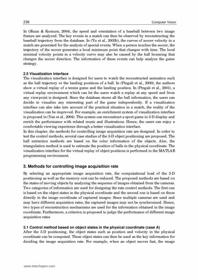
In (Shum & Komura, 2004), the speed and orientation of a baseball between two image
frames are analyzed. The key events in a match can then be observed by reconstructing the
baseball trajectory from the database. In (Yu et al., 2003b), the curves of soccer velocity in a
match are generated for the analysis of special events. When a person touches the soccer, the
trajectory of the soccer generates a local minimum point that changes with time. The local
minimal velocity points in a velocity curve may also be caused by the ball bouncing that
changes the soccer direction. The information of these events can help analyze the game
strategy.
2.5 Visualization interface The visualization interface is designed for users to watch the reconstructed animation such
as the ball trajectory or the landing positions of a ball. In (Pingali et al., 2000), the authors
show a virtual replay of a tennis game and the landing position. In (Pingali et al., 2001), a
virtual replay environment which can let the users watch a replay at any speed and from
any viewpoint is designed. Since the database stores all the ball information, the users can
decide to visualize any interesting part of the game independently. If a visualization
interface can also take into account of the practical situation in a match, the reality of the
visualization can be improved. For example, an enrichment system of visualization interface
is proposed in (Yan et al., 2004). This system can reconstruct a sport game in 3-D display and
enrich the performance with related music and illustrations. Hence, the users can enjoy a
comfortable viewing experience through a better visualization interface.
In this chapter, the methods for controlling image acquisition rate are designed. In order to
test the control methods, several case studies of the 3-D object positioning are proposed. The
ball extraction methods are based on the color information of the objects. Also, the
triangulation method is used to estimate the position of balls in the physical coordinate. The
visualization interface for the virtual replay of object positions is performed in the MATLAB
programming environment.
3. Methods for controlling image acquisition rate
By selecting an appropriate image acquisition rate, the computational load of the 3-D
positioning as well as the memory cost can be reduced. The proposed methods are based on
the states of moving objects by analyzing the sequence of images obtained from the cameras.
Two categories of information are used for designing the rate control methods. The first one
is based on the object states in the physical coordinate and the second one is based on those
directly in the image coordinate of captured images. Since multiple cameras are used and
may have different acquisition rates, the captured images may not be synchronized. Hence,
two types of reconstruction mechanisms are used for the information obtained in the image
coordinate. Furthermore, a criterion is proposed to judge the performance of different image
acquisition rates
3.1 Control method based on object states in the physical coordinate (case A) After the 3-D positioning, the object states such as position and velocity in the physical
coordinate can be computed. These object states can then be used as the key information for
deciding the image acquisition rate. For example, when an object moves fast, the image
www.intechopen.com

Image Acquisition Rate Control Based on Object State Information in Physical and Image Coordinates
237
acquisition rate should be set as high as possible to capture the object motion clearly. If an
object moves slowly or is only in a stationary status, a high acquisition rate is not required.
Using a high acquisition rate may waste the memory storage and the computational cost in
image processing. On the other hand, using a low acquisition rate may lose the reality of the
object motion. Hence, in order to balance the tradeoff between the computational cost and
the accuracy of the 3-D positioning result, the control method for adjusting different image
acquisition rates should be properly designed.
The proposed procedure is discussed in detail in the following. First of all, images are
captured by multiple cameras. Since the quality of captured images may be influenced by
noise, a spatial Gaussian filter is then used to smooth the captured images within the RGB
color channels. Based on a set of predefined features of the objects in terms of the RGB color
channels, the moving objects can be extracted from the images. After the objects are
extracted, the region occupied by the objects in a captured image is stored in a new gray-
scale image. These gray-scale images can be further transformed into binary images by a
specific threshold value. Some lighting influences on the objects may change the result of
color analysis on the object surfaces. The object surfaces in the binary image might not be
necessarily shown in a regular shape. Hence, the image dilation method can be used to
enlarge the analyzed image area, and to improve the object shapes in these binary images.
Finally, by the triangulation approach on the images, a set of 3-D information about the
objects in the physical coordinate can be computed. Also, since the time of captured images
and the corresponding estimated object position are recorded, the object velocity in the
physical domain can be estimated. By analyzing the position and velocity of the object, the
image acquisition rate for the next frame can then be adjusted based on the computed
information.
In this case (named as Case A), the key feature of controlling the image acquisition rate is to
analyze the object states in the physical coordinate. Assume that there are N levels of image
acquisition rates, and each level only represents a specific range of values for the object
states. Hence, by analyzing these object states, a corresponding image acquisition rate can be
determined. Figure 4 shows an example of the mapping between the ball velocity (i.e., the
object state) and the set of image acquisition rates. V0, V1, V2 ,…, VN, are the values of ball
velocity in the physical coordinate. Rate 1, Rate 2, …, Rate N, are different levels of image
acquisition rates arranged from the lowest value to the highest value. By analyzing the ball
velocity, the corresponding image acquisition rate can be determined. That is, if the ball
velocity is between Vi-1 and Vi, the corresponding image acquisition rate is set as Rate i.
…………………………………
Ball Velocity
(Slowest ) (Fastest)
Rate 2 Rate 3 Rate N
V1 V2 V3VN-1 VN
……
V0
Rate 1
Fig. 4. An example of mapping different image acquisition rates by the ball velocity (object
state)
www.intechopen.com
Computer Vision
238
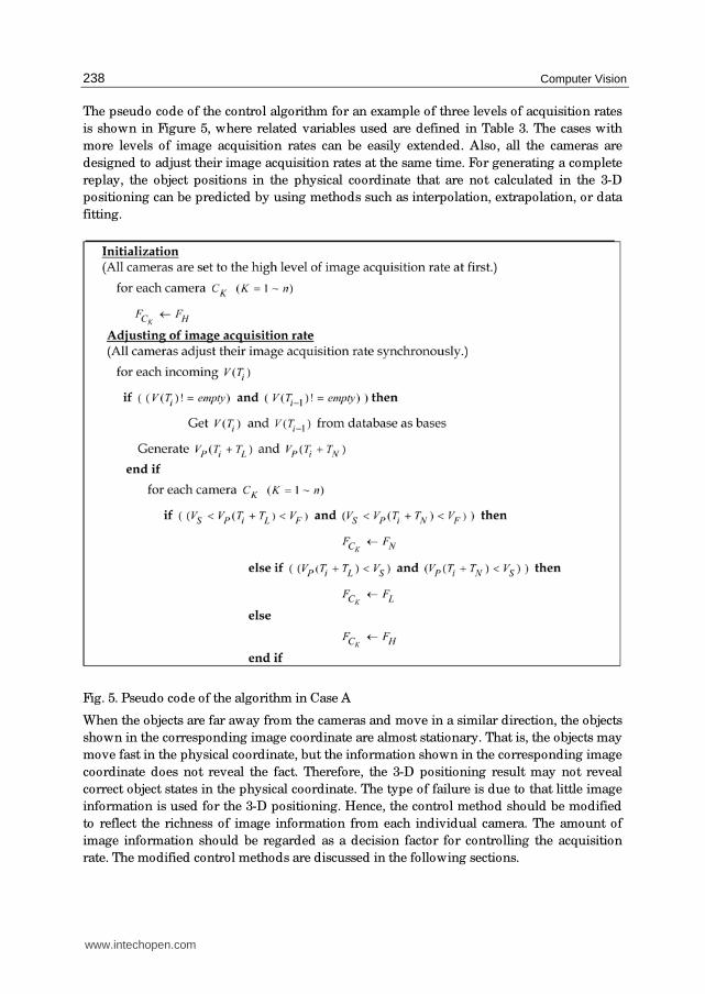
The pseudo code of the control algorithm for an example of three levels of acquisition rates
is shown in Figure 5, where related variables used are defined in Table 3. The cases with
more levels of image acquisition rates can be easily extended. Also, all the cameras are
designed to adjust their image acquisition rates at the same time. For generating a complete
replay, the object positions in the physical coordinate that are not calculated in the 3-D
positioning can be predicted by using methods such as interpolation, extrapolation, or data
fitting.
Fig. 5. Pseudo code of the algorithm in Case A
When the objects are far away from the cameras and move in a similar direction, the objects
shown in the corresponding image coordinate are almost stationary. That is, the objects may
move fast in the physical coordinate, but the information shown in the corresponding image
coordinate does not reveal the fact. Therefore, the 3-D positioning result may not reveal
correct object states in the physical coordinate. The type of failure is due to that little image
information is used for the 3-D positioning. Hence, the control method should be modified
to reflect the richness of image information from each individual camera. The amount of
image information should be regarded as a decision factor for controlling the acquisition
rate. The modified control methods are discussed in the following sections.
www.intechopen.com

Image Acquisition Rate Control Based on Object State Information in Physical and Image Coordinates
239
Symbol Definition Unit
KC index of camera ( 1 ~ )K n= none
KCF the image acquisition rate for the specific index of camera times/ sec
max( )KC
F the maximum image acquisition rate of the all cameras
KC ( 1 ~ )K n=
times/ sec
LF the specific low level of image acquisition rate times/ sec
NF the specific normal level of image acquisition rate times/ sec
HF the specific high level of image acquisition rate times/ sec
iT the recorded time of the captured image which is index i sec
LT
the corresponding image acquisition time to the lower level of
image acquisition rate ( 1 / )L LT F= sec
NT
the corresponding image acquisition time to the normal level of
image acquisition rate ( 1 / )N NT F= sec
( )P t the object velocity in the pixel coordinate domain at time t pixel/ sec
( )KC
PP t
the predictive object velocity in the image domain at time t (the
subscript K
C means the index of camera) pixel/ sec
SP the threshold value of slow object velocity in the image domain pixel/ sec
FP the threshold value of fast object velocity in the image domain pixel/ sec
( )V t the object velocity in the physical coordinate at time t mm/ sec
( )P
V t the predictive object velocity in the physical coordinate at time
t mm/ sec
SV
the threshold value of slow object velocity in the physical
coordinate mm/ sec
FV
the threshold value of fast object velocity in the physical
coordinate mm/ sec
Table 3. The meanings of the symbols in the control algorithm
3.2 Control method based on object states in the image coordinate (case B and case C) In Case A, the method for controlling the image acquisition rate is based on the object states
in the physical coordinate. In this section, novel methods to control the image acquisition
rate directly based on the object states in the image coordinate are proposed. The reason of
using the object states in the image coordinate is that the acquisition rates can be effectively
adjusted based on the actual available information instead of the projected information in
the physical coordinate. Based on different synchronization scenarios among the cameras,
two cases for adjusting the image acquisition rates are discussed. In the first case (named as
Case B), each camera adjusts the image acquisition rate independently to other cameras,
while in the second case (named as Case C) all the cameras adjust their image acquisition
rates cooperatively.
www.intechopen.com

Computer Vision
240
3.2.1 Independently controlling image acquisition rate (case B) In Case B, each camera is designed to control its image acquisition rate independently based
on the information in the image coordinate. The object states are first analyzed
independently in the image coordinate of each camera and then each camera adjusts the
acquisition rate based on the significance of the analyzed image. The significance can be
used as a function of the mobility or the geometric feature of the object. Since all the cameras
do not capture image simultaneously, the numbers of captured images at each camera are
neither the same nor synchronized. Hence, during the 3-D reconstruction, the images from
some cameras may be missed. To overcome this drawback, an interpolation or extrapolation
method should be applied for those missing images. The advantage of only capturing the
most significant images is to reduce the computational load for reconstructing useless
images in the physical coordinate, and/ or the transmission bandwidth. The algorithm for
the adjustment of three-level image acquisition rates is shown in Figure 6. The definition of
the variables in the algorithm is also listed in Table 3. Cases with more levels of image
acquisition rates can be easily extended.
Fig. 6. Pseudo code of the algorithm in Case B
In Case A, all the cameras adjust their image acquisition rates simultaneously, so that the
captured images are always in pairs for further processing. Hence, the object states in the
www.intechopen.com

Image Acquisition Rate Control Based on Object State Information in Physical and Image Coordinates
241
physical coordinate can be directly reconstructed. In Case B, since these cameras adjust their
image acquisition rate independently, the acquisition efficiency of each camera could be
improved, but the captured images may not be necessarily in pairs. The missing images can
be recovered by an interpolation or extrapolation estimation based on the captured images.
Therefore, the 3-D reconstruction of the objects in the physical coordinate can also be
performed.
However, in some scenarios, if the reconstruction by interpolation or extrapolation
generates unacceptable errors, it is advised to increase the acquisition rates of some cameras
in a cooperative way. The cooperation increases the acquisition rates of some cameras and
hence improves the reconstruction performance. However, the total number of captured
images is still smaller than that in Case A. Therefore, the computational cost is still reduced.
The cooperation mechanism is discussed in next section.
3.2.2 Cooperatively controlling image acquisition rates (case C) In this case, the method for controlling image acquisition rate is also based on the
information obtained in the image coordinate. In additions, all cameras try to adjust its
image acquisition rate synchronously. In order to achieve the synchronization, these
acquisition rates should first be compared. The comparison works as follows. Each camera
first predicts an image acquisition rate for the next image frame. The control algorithm then
compares the prediction of each camera and then a designated image acquisition rate is
chosen as the highest of all the predicted image acquisition rates. Finally, all the cameras
adjust to their acquisition rates synchronously. Therefore, the captured images from all the
cameras can be used for the 3-D reconstructions simultaneously.
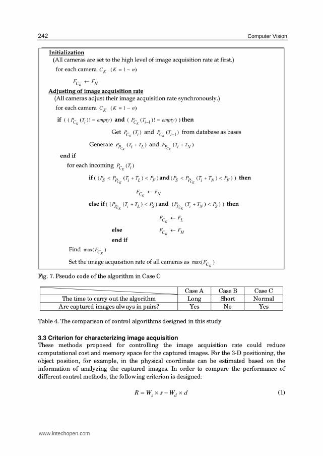
The algorithm for the case of three levels of image acquisition rates is shown in Figure 7.
The definition of the variables in the algorithm is also listed in Table 3. Cases with more
levels of image acquisition rates can be easily extended. Initially, all the cameras are set to
the higher level of image acquisition rate and, hence, capture some images in the meantime.
Therefore, the set of captured images are in pairs. After that, the image is further analyzed
and, because the image information obtained is different among these cameras, each camera
may adjust its acquisition rate independently. Next, at each camera, the image acquisition
rate for the next image frame is analyzed and predicted based on the captured images. In
order to capture the next image frame synchronously, all the cameras are adjusted to the
highest level of all the predicted image acquisition rates and the image frames can be
guaranteed to be captured at the same time.
By using this algorithm, the cameras can compare their predicted image acquisition rates
and adopt the highest rate for the next image frame. Since the algorithm in Case C adjusts
the image acquisition rate before analyzing the object information in the physical
coordinate, this algorithm could performs more efficiently than that of Case A. A
preliminary comparison of the three control algorithms is listed in Table 4.
In addition to the synchronization effect and reconstruction performance, other factors can
also be considered when selecting a suitable algorithm for controlling the image acquisition
rate. The most important concept is that the adjustment of the acquisition rate should
depend on the image quality captured by each camera. In order to characterize the outcome
of the proposed control methods, a performance criterion is proposed in the next section.
www.intechopen.com
Computer Vision
242
Fig. 7. Pseudo code of the algorithm in Case C
Case A Case B Case C
The time to carry out the algorithm Long Short Normal
Are captured images always in pairs? Yes No Yes
Table 4. The comparison of control algorithms designed in this study
3.3 Criterion for characterizing image acquisition These methods proposed for controlling the image acquisition rate could reduce
computational cost and memory space for the captured images. For the 3-D positioning, the
object position, for example, in the physical coordinate can be estimated based on the
information of analyzing the captured images. In order to compare the performance of
different control methods, the following criterion is designed:
s dR W s W d= × − × (1)
www.intechopen.com

Image Acquisition Rate Control Based on Object State Information in Physical and Image Coordinates
243
where s denotes the saving percentage of image quantity, d denotes a reference value
representing the percentage of image distortion, and ,s d
W W are two weighting factors.
Specifically, s can be described as follows:
1
2
1 ,N
sN
= − (2)
where N1 denotes the number of captured images when carrying out the control method and
N2 denotes the number of captured images when all the cameras are set at the highest
acquisition rate. For example, if 240 images are captured using the highest acquisition rate,
and only 200 images are recorded by performing one of control methods, then the
percentage of image saving is estimated as follows:
2001 0.167 16.7%.
240s = − ≅ =
Furthermore, sW can be regarded as a function of memory saving. For example, the function
can be defined as follows:
( ),sW α ξ= (3)
where 1 2/M Mξ = and
1M denotes the quantity of memory used to record all the captured
images by using the highest acquisition rate, and 2M denotes the quantity of memory
assigned by the computer in advance. For example, if it needs 100MB to record all the
captured images and the memory size assigned by the computer is 80MB, ξ can be
calculated as follows:
1001.25.
80ξ = =
If 1ξ > , then saving the number of captured images can be considered an important goal.
dW can be regarded as a function of the object states and the image acquisition rate. For
example, dW is described as follows:
( , ),d
W v kβ= (4)
where v characterizes the object states such as position or velocity, and k is the highest
acquisition rate used in a practical application. If the object states have a large impact on the
image processing (for example, the object speed is large), and the image acquisition rate is
low, it is likely that the outcome of the image processing will be distorted and the value of
dW should be increased. In summary, sW s× can be regarded as the advantage for carrying
out the control method, while d
W d× can be regarded as the disadvantage for carrying out
the control method.
www.intechopen.com

Computer Vision
244
When the value of R is equal to zero, the performance of the control method is just the same
as that without any acquisition rate control because all the images are just captured by the
highest image acquisition rate and occupy all the available memory. Hence, in order to
guarantee the performance of the control method, the value of R should be a positive
number. If several control methods are available for the users to choose, they can be
compared based on the criterion.
4. Experimental results
In this section, the 3-D positioning of solid balls are experimentally tested for the three
methods of controlling image acquisition rates. The test-bed is shown in Figure 8(a). The
image coordinates of the two cameras is shown in Figure 8(b), where the camera centers are
denoted as P1 and P2, respectively, and π1 and π2 are the image frames of the two camera,
repsectively. Since three balls of different colors are used in these experiments, the
foreground object segmentation can be easily performed. The background of the scene is
only white broads. Also, two cameras are used to capture the images which are stored and
analyzed at one single computer.
P1
P2
Camera I
Camera II
P1
P2
P1
P2
Camera I
Camera II
P1Pf
f
+Y
f
f
+Z
P2
+X
1π
2π
(a) (b)
Fig. 8. (a) A snapshot of experimental environment for 3-D positioning, (b) the image
coordinates of the two cameras
In this study, assume that the radius of these balls is known in advance. Hence, the goal of
the 3-D positioning is only to identify the center of these balls. In order to locate the ball
centers in the physical coordinate, the ball center shown in each camera should be processed
first by proper image processing operations. Once the position of the ball center in the image
coordinate of each camera is found, the position of ball center in the physical coordinate can
then be computed by the triangulation method used in the 3-D mapping.
4.1 Image processing results The captured images are stored in the memory of the computer and processed by the image
processing step. First of all, the original captured images loaded from the memory are full-
color images, i.e., with red, green and blue color channels. The spatial Gaussian filter is then
used to process these color channels, independently. In order to distinguish these three balls
shown in the image, each ball is identified from the image by the color analysis. Supposing
www.intechopen.com

Image Acquisition Rate Control Based on Object State Information in Physical and Image Coordinates
245
that a ball region is extracted after the color analysis, the region is stored and transformed
into a gray-scale image. The gray-scale image can be further transformed into a binary
image. Finally, the image dilation method is used to further characterize the shape of ball
region shown in the binary image.
In the color analysis step, all pixels in a captured image are processed by a color analysis
method. That is, a pixel shown in the captured images can be judged as either a part of color
ball or a part of background. When a pixel does not belong to the region of the three balls,
the pixel is regarded as a part of background. This color analysis method is designed to
process all pixels in the captured image. Supposing that the balls are not blocked by others,
this color analysis method can identify every ball region. An example of using the color
analysis method to find a ball region is shown in Figure 9.
In Figure 9(a), an original captured image is shown. Next, the extraction result of the green ball is shown in Figure 9(b), where a binary image is obtained. It is clear that the ball shape is incorrect after the color analysis. Hence, the image dilation method is used to further improve the result of ball region extraction. The result after the image dilation is shown in Figure 9(c), where the ball shape is better than that shown in Figure 9(b).
(a)
(b) (c)
Fig. 9. The results of ball extraction and image dilation in the captured image. (a) The
original image. (b) After ball extraction. (c) After image dilation
4.2 3-D positioning results In this study, the target for 3-D positioning are the centers of the balls. In order to find the
positions of ball centers in the physical domain, the ball centroid shown in images are first
www.intechopen.com

Computer Vision
246
calculated by the image processing step discussed in previous section. Once the positions of
ball centroid shown in images are found, the position of ball center in the physical domain
can be found by the triangulation method. Supposing that a ball center s is the target for 3-
D positioning, an example of the corresponding points of s in the image planes of the two
cameras used in this study is shown in Figure 10.
1π 2π(160,120) (160,120)
f f1T 2T
1P 2P1X+ 2X+
1Y+ 2Y+
1Z+ 2Z+
x+ x+y+ y+ Pixel Coordinate
Frame
Camera Coordinate
Frame
Pixel Coordinate
Frame
Camera Coordinate
Frame
1s
2s
s
xx
y y
x1
y1
x2
y2
Domain Domain
Pixel Coordinate Domain
Pixel Coordinate Domain1π 2π(160,120) (160,120)
f f1T 2T
1P 2P1X+ 2X+
1Y+ 2Y+
1Z+ 2Z+
x+ x+y+ y+ Pixel Coordinate
Frame
Camera Coordinate
Frame
Pixel Coordinate
Frame
Camera Coordinate
Frame
1s
2s
s
xx
y y
x1
y1
x2
y2
Domain Domain
Pixel Coordinate Domain
Pixel Coordinate Domain
Fig. 10. An example for describing the corresponding points of a ball center in the image
planes
The centers of the two camera coordinate domains are denoted by P1 and P2, respectively,
and the image planes are denoted by π1 and π2, respectively. Assume that the range of the
image plane is 320*240 in pixel and the center of the image coordinate is then denoted as
(160, 120). The focal length is denoted by f. The ball center s is the target of the 3-D
positioning, and the corresponding point of s shown in the two image coordinates are
denated as s1 and s2, respectively. Hence, the coordinates of s1 and s2 in π1 and π2,
respevtively, can be described as follows:
1 1 1( , )s x y= (5)
2 2 2( , )s x y= (6)
Supposing that the unit of the focal length f is in terms of pixel, the two 3-D vectors T1 and
T2 can be described as follows
1 1 1( 160, 120, )T x y f= − − (6)
2 2 2( 160, 120, )T x y f= − − (7)
www.intechopen.com
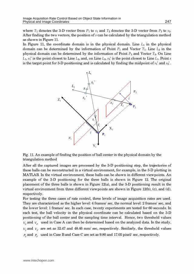
Image Acquisition Rate Control Based on Object State Information in Physical and Image Coordinates
247
where T1 denotes the 3-D vector from P1 to s1 and T2 denotes the 3-D vector from P2 to s2.
After finding the two vectors, the position of s can be calculated by the triangulation method
as shown in Figure 11.
In Figure 11, the coordinate domain is in the physical domain. Line L1 in the physical
domain can be determined by the information of Point P1 and Vector T1. Line L2 in the
physical domain can be determined by the information of Point P2 and Vector T2. On Line
L1, s1’ is the point closest to Line L2, and, on Line L2, s2’ is the point closest to Line L1. Point s
is the target point for 3-D positioning and is calculated by finding the midpoint of s1’ and s2’ .
P1Pf
f
+Y1
f
f
+Z1
P2
+X1
1π
2π
1L
2L
1T
2T
1s
2s
'
1s
'
2s
s
X1
Y1
Z1
1 's
2 's
Fig. 11. An example of finding the position of ball center in the physical domain by the
triangulation method
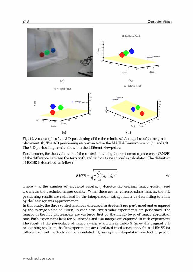
After all the captured images are processed by the 3-D positioning step, the trajectories of
these balls can be reconstructed in a virtual environment, for example, in the 3-D plotting in
MATLAB. In the virtual environment, these balls can be shown in different viewpoints. An
example of the 3-D positioning for the three balls is shown in Figure 12. The original
placement of the three balls is shown in Figure 12(a), and the 3-D positioning result in the
virtual environment from three different viewpoints are shown in Figure 12(b), (c), and (d),
respectively.
For testing the three cases of rate control, three levels of image acquisition rates are used.
They are characterized as the higher level: 4 frames/ sec, the normal level: 2 frames/ sec, and
the lower level: 1 frames/ sec. In each case, twenty experiments are tested for 60 seconds. In
each test, the ball velocity in the physical coordinate can be calculated based on the 3-D
positioning of the ball center and the sampling time interval. Hence, two threshold values
SV and
FV used in Case A can then be determined based on the analyzed data. In the study,
SV and
FV are set as 32.47 and 48.46 mm/ sec, respectively. Similarly, the threshold values
SP and
FP used in Case B and Case C are set as 9.80 and 17.05 pixel/ sec, respectively.
www.intechopen.com
Computer Vision
248
-100
10 20
020
4060
80
-15
-10
-5
0
5
10
15
camera
X-axis
camera
3D Positioning Result
Z-axis
Y-a
xis
(a) (b)
-1001020
0
20
40
60
80
-15
-10
-5
0
5
10
15
cameracamera
3D Positioning Result
Z-axis
X-axis
Y-a
xis
-100
1020
0
20
40
60
80
-15
-10
-5
0
5
10
15
X-axis Z-axis
3D Positioning Result
cameracamera
Y-a
xis
(c) (d)
Fig. 12. An example of the 3-D positioning of the three balls. (a) A snapshot of the original
placement. (b) The 3-D positioning reconstructed in the MATLAB environment. (c) and (d)
The 3-D positioning results shown in the different viewpoints
Furthermore, for the evaluation of the control methods, the root-mean-square-error (RMSE)
of the difference between the tests with and without rate control is calculated. The definition
of RMSE is described as follows:
2
1
1ˆ( )
n
i ii
RMSE q qn =
= −∑ (8)
where n is the number of predicted results, q denotes the original image quality, and
q̂ denotes the predicted image quality. When there are no corresponding images, the 3-D
positioning results are estimated by the interpolation, extrapolation, or data fitting to a line
by the least squares approximation.
In this study, the three control methods discussed in Section 3 are performed and compared
by the average value of RMSE. In each case, five similar experiments are performed. The
images in the five experiments are captured first by the higher level of image acquisition
rate. Each experiment lasts for 60 seconds and 240 images are captured in each experiment.
The result of the percentage of image saving is shown in Table 5. Since the original 3-D
positioning results in the five experiments are calculated in advance, the values of RMSE for
different control methods can be calculated. By using the interpolation method to predict
www.intechopen.com

Image Acquisition Rate Control Based on Object State Information in Physical and Image Coordinates
249
unknown 3-D positions, the calculated results for RMSE is shown in Table 6. By using the
extrapolation method to predict unknown 3-D positions, the calculated results for RMSE is
shown in Table 7. Finllay, by using the method of least squares approximation to predict
unknown 3-D positions, the calculated results for RMSE is shown in Table 8. Also, the
timing data of the image acquisition by uisng the three control methods and the fixed rate
cases are shown in Figure 13.
When all the images are captured by a fixed, normal image acquisition rate, the percentage
of image saving is the smallest. In Case C, the image acquisition rate is adjusted before
comparing the image processing result of the two cameras. Once one camera determines the
time to capture next image, the other camera also capture the image no matter what its
original decision is. Hence, the percentage of image saving for Case C is smaller than that of
Case A and Case B.
For the prediction performance, since Case C acquires more images than Case A and Case B
do, the RMSE for Case C are smaller than those for Case A and Case B. In Case B, the two
cameras do not utilize identical image acquisition rate synchronously. Hence, the position of
the ball in the image coordinate is then predicted. In Case A and Case B, the image
acquisition rate for the two cameras is adjusted synchronously. Therefore, the RMSE in Case
B is larger than those Case A and Case C.
Percentage of image saving
Index of
experiments Case A Case B Case C
Fixed rate
(normal level)
Fixed rate
(lower level)
1 71.67% 70.42% 52.08% 50% 75%
2 71.67% 70.21% 54.58% 50% 75%
3 72.50% 70.21% 56.67% 50% 75%
4 72.92% 70.63% 63.75% 50% 75%
5 72.92% 68.13% 52.08% 50% 75%
Average 72.34% 69.92% 55.83% 50% 75%
Table 5. The percentage of image saving in the experiments
RMSE (by the interpolation method) (Unit: mm)
Index of
experiments Case A Case B Case C
Fixed rate
(normal level)
Fixed rate
(lower level)
1 32.122 63.279 25.957 22.951 33.863
2 33.417 54.744 33.129 22.347 35.781
3 29.328 47.472 26.531 20.588 30.771
4 33.403 68.569 32.773 23.019 34.769
5 31.169 109.168 27.352 21.224 32.368
Average 31.888 68.646 29.142 22.026 33.510
Table 6. The RMSE of prediction performance when all unknown 3-D positioning results are
predicted by the interpolation method
www.intechopen.com

Computer Vision
250
RMSE (by the extrapolation method) (Unit: mm)
Index of
experiments Case I Case II Case III
Fixed rate
(normal level)
Fixed rate
(lower level)
1 56.811 148.509 57.446 43.265 59.658
2 67.293 103.541 63.782 44.111 63.331
3 60.500 109.406 57.555 36.308 55.947
4 59.374 134.716 67.257 41.649 55.583
5 61.874 225.318 58.105 39.891 61.883
Average 61.170 144.298 60.229 41.045 59.280
Table 7. The RMSE of prediction performance when all unknown 3-D positioning results are
predicted by the extrapolation method
RMSE (by the method of data fitting to a line) (Unit: mm)
Index of
experiments Case A Case B Case C
Fixed rate
(normal level)
Fixed rate
(lower level)
1 56.628 122.772 51.346 39.219 56.959
2 62.361 103.874 63.106 41.516 59.385
3 57.299 102.364 52.468 36.267 53.805
4 59.218 136.043 59.807 38.435 54.829
5 56.965 210.031 53.714 41.380 56.788
Average 58.494 135.017 56.088 39.363 56.353
Table 8. The RMSE of prediction performance when all unknown 3-D positioning results are
predicted by the method of data fitting to a line
Finally, the performance criterion, defined in Section 3.3, of these three cases is summarized
in Table 9. The performance criteria in Case A are larger than those in Case B and Case C.
Hence, the performance of Case A is the best. Also, it is advised to use a control method
with a positive R. Therefore, the performance of Case B is not good enough. Also, the
statistic suggests that the performance of using interpolation to predict the missing data is
better than that of using extrapolation and data fitting.
R
Case A Case B Case C
Interpolation 0.2440 -0.1614 0.1139
Extrapolation -0.1842 -1.0421 -0.3477
Data fitting -0.1520 -0.9354 -0.2723
Table 9. The performance criterion R
In summary, Case A has a better result in the percentage of image saving and the
performance criterion. For Case B, due to the asynchronization in image acquisition, the 3-D
www.intechopen.com

Image Acquisition Rate Control Based on Object State Information in Physical and Image Coordinates
251
positioning results cannot be predicted properly and may generate bigger errors than that in
Case A and Case C. Therefore, if the cameras can be placed in an appropriate position to
avoid the problem of obtaining too little object information, Case A should be a better choice
for practical application than Case C.
0 10 20 30 40 50 600
1
2
3
4
5
6
7
Time (sec)
Index o
f D
iffe
rent
Ca
ses
Compare the control methods with the cases of fixed rate
Y-Axis Index- "1"--Fixed Rate(All Higher Level)
Y-Axis Index- "2"--Fixed Rate(All Normal Level)
Y-Axis Index- "3"--Fixed Rate(All Lower Level)
Y-Axis Index- "4"-- Case I
Y-Axis Index- "5"-- Case II
Y-Axis Index- "6"-- Case III
0 10 20 30 40 50 60
0
1
2
3
4
5
6
7
Time (sec)
Index o
f D
iffe
rent
Cases
Compare the control methods with the cases of fixed rate
Y-Axis Index- "1"--Fixed Rate(All Higher Level)
Y-Axis Index- "2"--Fixed Rate(All Normal Level)
Y-Axis Index- "3"--Fixed Rate(All Lower Level)
Y-Axis Index- "4"-- Case I
Y-Axis Index- "5"-- Case II
Y-Axis Index- "6"-- Case III
(a) (b)
0 10 20 30 40 50 600
1
2
3
4
5
6
7
Time (sec)
Index o
f D
iffe
rent
Cases
Compare the control methods with the cases of fixed rate
Y-Axis Index- "1"--Fixed Rate(All Higher Level)
Y-Axis Index- "2"--Fixed Rate(All Normal Level)
Y-Axis Index- "3"--Fixed Rate(All Lower Level)
Y-Axis Index- "4"-- Case I
Y-Axis Index- "5"-- Case II
Y-Axis Index- "6"-- Case III
0 10 20 30 40 50 60
0
1
2
3
4
5
6
7
Time (sec)
Index o
f D
iffe
rent
Cases
Compare the control methods with the cases of fixed rate
Y-Axis Index- "1"--Fixed Rate(All Higher Level)
Y-Axis Index- "2"--Fixed Rate(All Normal Level)
Y-Axis Index- "3"--Fixed Rate(All Lower Level)
Y-Axis Index- "4"-- Case I
Y-Axis Index- "5"-- Case II
Y-Axis Index- "6"-- Case III
(c) (d)
0 10 20 30 40 50 600
1
2
3
4
5
6
7
Time (sec)
Index o
f D
iffe
rent
Cases
Compare the control methods with the cases of fixed rate
Y-Axis Index- "1"--Fixed Rate(All Higher Level)
Y-Axis Index- "2"--Fixed Rate(All Normal Level)
Y-Axis Index- "3"--Fixed Rate(All Lower Level)
Y-Axis Index- "4"-- Case I
Y-Axis Index- "5"-- Case II
Y-Axis Index- "6"-- Case III
(e)
Fig. 13. The timing comparison for different image acquisition mechanisms by using the
three control methods and the fixed rate cases. (a)-(e) The five experiments performed
5. Conclusions and future work
In this study, three methods for controlling image acquisition rate are designed and
analyzed. In order to verify the control methods, the 3-D positioning of balls is used to
compare the performance of the three control methods in terms of the percentage of saving
images and the accuracy of the 3-D positioning results. Experimental results show that the
www.intechopen.com

Computer Vision
252
calculating results for the percentage of saving images in Case C is smaller than that in Case
A and Case B. However, since Case C adopts more images to predict the motion of the balls
in the physical domain, the accuracy of the 3-D positioning result in Case C is better than
that in Case A and Case B. The accuracy for the 3-D positioning result for Case B is worse
than that in Case A and Case C. In order to compare the performance of the three cases, a
performance criterion for judging these control methods is proposed. In practical
applications, cameras should be placed or moved in an appropriate position to avoid the
problem of getting too little object information from the images.
In the future, the following three tasks can be further performed. The first task is to use
advanced mathematical methods for predicting the positions of the interested objects in
the physical domain. The second task is to design more advanced control methods for
better characterize the object states. The third task is to test the scenarios with more
cameras and interested objects for testing the complexity achieved by the proposed
control methods.
6. Acknowledgement
This work was supported in part by the National Science Council, Taiwan, ROC, under the
grants: NSC 95-2221-E-002-303-MY3, and NSC 96-2218-E-002-030, and by DOIT/ TDPA: 96-
EC-17-A-04-S1-054.
7. References
Andrade, E.L.; Woods, J.C.; Khan, E. & Ghanbrai M. (2005) Region-Based Analysis and
Retrieval for Tracking of Semantic Objects and Provision of Augmented
Information in Interactive Sport Scenes, IEEE Transactions on Multimedia, Vol. 7, No.
6, (Dec. 2005) pp. 1084-1096, ISSN: 1520-9210
D’Orazio, T.; Ancona, N.; Cicirelli, G. & Nitti, M. (2002) A Ball Detection Algorithm for Real
Soccer Image Sequences, Proceedings of the 16th International Conference on Pattern
Recognition, pp. 210-213, ISBN: 0-7695-1685-x, Quebec, Canada, Aug. 2002, Institute
of Electrical and Electronics Engineers, Piscataway
Hong, S.M. (2002) Steady-State Analysis of Computational Load in Correlation-Based Image
Tracking, IEE Proceedings on Vision, Image, and Signal Processing, Vol. 149, No. 3,
(June 2002) pp. 168-172, ISSN: 1350-245X
Iwase, H. & Murata A. (2001) Discussion on Skillful Baseball Pitch Using Three-Dimensional
Cinematographic Analysis. Comparison of Baseball Pitch between Skilled and
Unskilled Pitchers, Proceedings of the IEEE International Conference on Systems, Man,
and Cybernetics, pp. 34-39, ISBN: 0-7803-7087-2, Tucson, AZ, USA, Oct. 2001,
Institute of Electrical and Electronics Engineers, Piscataway
Ohno, Y.; Miura, J. & Shirai Y. (2000) Tracking Players and Estimation of the 3D Position of a
Ball in Soccer Games, Proceedings of the IEEE International Conference on Pattern
Recognition, pp. 145-148, ISBN: 0-7695-0750-6, Barcelona, Spain, Sep. 2000, Institute
of Electrical and Electronics Engineers, Piscataway
Pingali, G.; Opalach, A.; Jean, Y. & Carlbom, I. (2001) Visualization of Sports Using Motion
Trajectories: Providing Insights into Performance, Style, and Strategy, Proceedings of
www.intechopen.com
Image Acquisition Rate Control Based on Object State Information in Physical and Image Coordinates
253
the IEEE International Conference on Visualization, pp. 75-82, ISBN: 0-7803-7200-x, San
Diego, CA, USA, Oct. 2001, Institute of Electrical and Electronics Engineers,
Piscataway
Pingali, G.; Opalach, A. & Jean, Y. (2000) Ball Tracking and Virtual Replays for Innovative
Tennis Broadcasts, Proceedings of the IEEE International Conference on Pattern
Recognition, pp. 152-156, ISBN: 0-695-0750-6, Barcelona, Spain, Sep. 2000, Institute of
Electrical and Electronics Engineers, Piscataway
Ren, J.; Orwell, J.; Jones, G.A. & Xu, M. (2004) A General Framework for 3D Soccer Ball
Estimation and Tracking, Proceedings of the IEEE International Conference on Image
Processing, pp. 1935-1938, ISBN: 0-7803-8554-3, Genova, Italy, Oct. 2004, Institute of
Electrical and Electronics Engineers, Piscataway
Shah, H. & Morrell, D. (2004) An Adaptive Zoom Algorithm for Tracking Targets Using
Pan-Tilt-Zoom Cameras, Proceedings of the IEEE International Conference on Acoustics,
Speech, and Signal Processing, pp. 17-21, ISBN: 0-7803-8484-9, Quebec, Canada, May
2004, Montreal, Institute of Electrical and Electronics Engineers, Piscataway
Shin, B.S. & Shin, Y.G. (1998) Fast 3D Solid Model Reconstruction from Orthographic Views,
Computer-Aided Design, Vol. 30, No. 1, (Jan. 1998) pp. 63-76, ISSN: 0010-4485
Shum, H. & Komura, T. (2004) A Spatiotemporal Approach to Extract the 3D Trajectory of
the Baseball from a Single View Video Sequence, Proceedings of the IEEE
International Conference on Multimedia and Expo, pp. 1583-1586, ISBN: 0-7803-8603-5,
Taipei, Taiwan, June 2004, Institute of Electrical and Electronics Engineers,
Piscataway
Theobalt, C.; Albrecht, I.; Haber, J.; Magnor, M. & Seidel, H.P. (2004) Pitching a
Baseball: Tracking High-Speed Motion with Multi-Exposure Images, ACM
Transactions on Graphics, Vol. 23, No. 3, (Aug. 2004) pp. 540-547, ISSN: 0730-0301
Wang, C.K. ; Cheng, M.Y.; Liao, C.H.; Li, C.C.; Sun, C.Y. & Tsai, M.C. (2004) Design and
Implementation of a Multi-Purpose Real-Time Pan-Tilt Visual Tracking System,
Proceedings of the IEEE International Conference on Control Applications, pp. 1079-1084,
ISBN: 0-7803-8633-7, Taipei, Taiwan, Sep. 2004, Institute of Electrical and
Electronics Engineers, Piscataway
Yan, X.; Yu, X. & Hay, T.S. (2004) A 3D Reconstruction and Enrichment System for
Broadcast Soccer Video, Proceedings of the 12th ACM International Conference on
Multimedia, pp. 746-747, ISBN: 1-58113-893-8, New York, NY, USA, Oct. 2004,
Institute of Electrical and Electronics Engineers, Piscataway
Yu, X.; Xu, C.; Tian, Q. & Leong, H.W. (2003a) A Ball Tracking Framework for Broadcast
Soccer Video, Proceedings of the IEEE International Conference on Multimedia and Expo,
pp. 273-276, ISBN: 0-7803-7965-9, Baltimore, MD, USA, July 2003, Institute of
Electrical and Electronics Engineers, Piscataway
Yu, X.; Leong, H.W.; Lim, J.; Tian, Q. & Jiang, Z. (2003b) Team Possession Analysis for
Broadcast Soccer Video Based on Ball Trajectory, Proceedings of the IEEE
International Conference on Information, Communications and Signal Processing, pp.
1811-1815, ISBN: 0-7803-8185-8, Singapore, Dec. 2003, Institute of Electrical and
Electronics Engineers, Piscataway
www.intechopen.com

Computer Vision
254
Yu, X.; Sim, C.H.; Wang, J.R. & Cheong, L.F. (2004) A Trajectory-Based Ball Detection and
Tracking Algorithm in Broadcast Tennis Video, Proceedings of the IEEE International
Conference on Image Processing, pp. 1049-1052, ISBN: 0-7803-8554-3, Genova, Italy,
Oct. 2004, Institute of Electrical and Electronics Engineers, Piscataway
www.intechopen.com

Computer VisionEdited by Xiong Zhihui
ISBN 978-953-7619-21-3Hard cover, 538 pagesPublisher InTechPublished online 01, November, 2008Published in print edition November, 2008
InTech EuropeUniversity Campus STeP Ri Slavka Krautzeka 83/A 51000 Rijeka, Croatia Phone: +385 (51) 770 447 Fax: +385 (51) 686 166www.intechopen.com
InTech ChinaUnit 405, Office Block, Hotel Equatorial Shanghai No.65, Yan An Road (West), Shanghai, 200040, China
Phone: +86-21-62489820 Fax: +86-21-62489821
This book presents research trends on computer vision, especially on application of robotics, and on advancedapproachs for computer vision (such as omnidirectional vision). Among them, research on RFID technologyintegrating stereo vision to localize an indoor mobile robot is included in this book. Besides, this book includesmany research on omnidirectional vision, and the combination of omnidirectional vision with robotics. Thisbook features representative work on the computer vision, and it puts more focus on robotics vision andomnidirectioal vision. The intended audience is anyone who wishes to become familiar with the latest researchwork on computer vision, especially its applications on robots. The contents of this book allow the reader toknow more technical aspects and applications of computer vision. Researchers and instructors will benefit fromthis book.
How to referenceIn order to correctly reference this scholarly work, feel free to copy and paste the following:
Feng-Li Lian and Shih-Yuan Peng (2008). Image Acquisition Rate Control Based on Object State Informationin Physical and Image Coordinates, Computer Vision, Xiong Zhihui (Ed.), ISBN: 978-953-7619-21-3, InTech,Available from:http://www.intechopen.com/books/computer_vision/image_acquisition_rate_control_based_on_object_state_information_in_physical_and_image_coordinates

© 2008 The Author(s). Licensee IntechOpen. This chapter is distributedunder the terms of the Creative Commons Attribution-NonCommercial-ShareAlike-3.0 License, which permits use, distribution and reproduction fornon-commercial purposes, provided the original is properly cited andderivative works building on this content are distributed under the samelicense.