Federal Reserve Bank of MinneapolisResearch Department Staff Report 371

Revised August 2008

Time-Varying Risk, Interest Rates, andExchange Rates in General Equilibrium

Fernando Alvarez∗

University of Chicagoand National Bureau of Economic Research

Andrew Atkeson∗

University of California,Federal Reserve Bank of Minneapolis,and National Bureau of Economic Research

Patrick J. Kehoe∗

Federal Reserve Bank of Minneapolis,University of Minnesota,and National Bureau of Economic Research

ABSTRACT

Under mild assumptions, the data indicate that fluctuations in nominal interest rate differentialsacross currencies are primarily fluctuations in time-varying risk. This finding is an immediateimplication of the fact that exchange rates are roughly random walks. If most fluctuations ininterest differentials are thought to be driven by monetary policy, then the data call for a theorywhich explains how changes in monetary policy change risk. Here we propose such a theory basedon a general equilibrium monetary model with an endogenous source of risk variation–a variabledegree of asset market segmentation.

∗The authors thank George Marios Angeletos, Martin Boileau, Charles Engel, Michael Devereux, Pierre-OlivierGourinchas, Juan Pablo Nicolini, Pedro Teles, Chris Telmer, Linda Tesar, Jaume Ventura, and Ivan Werningfor helpful comments. The authors also thank the National Science Foundation for financial assistance andKathy Rolfe and Joan Gieseke for excellent editorial assistance. The views expressed herein are those of theauthors and not necessarily those of the Federal Reserve Bank of Minneapolis or the Federal Reserve System.

Overall, the new view of finance amounts to a profound change. We have to get

used to the fact that most returns and price variation comes from variation in

risk premia. (Cochrane 2001, p. 451)

Cochrane’s observation directs our attention to a critical counterfactual part of the standard

general equilibrium monetary model: constant risk premia. Variation in risk over time is

essential for understanding movements in asset prices; that has been widely documented.

Yet the standard model does not generate time-varying risk premia. We develop a simple,

general equilibrium monetary model that does. In our model, the asset market is segmented;

at any time, only a fraction of the model’s agents choose to participate in that market. Risk

premia in our model thus vary over time because the degree of asset market segmentation

varies over time, endogenously, in response to stochastic shocks.

We apply the model to interest rates and exchange rates because data on those vari-

ables provide some of the most compelling evidence that variation in risk premia is a prime

mover behind variation in asset prices. In fact, a stylized view of the data on interest rates and

exchange rates is that observed variations in interest rate differentials across bonds denomi-

nated in different currencies are accounted for almost entirely by variations in risk premia.

To make this view concrete, consider the risk, in nominal terms, faced by a U.S.

investor choosing between bonds denominated in either dollars or euros. Clearly, for this

investor, the dollar return on the euro bond is risky because next period’s exchange rate is

not known today. The risk premium compensates the investor who chooses to hold the euro

bond for taking on this exchange rate risk. Specifically, in logs, the risk premium pt is equal

to the expected log dollar return on a euro bond minus the log dollar return on a dollar bond,

pt = i∗t + Et log et+1 − log et − it,

where i∗t and it are the logs of euro and dollar gross interest rates and et is the exchange

rate between the currencies.1 The difference in nominal interest rates across currencies can

thus be divided into the expected change in the exchange rate between these currencies and

a currency risk premium.

In standard equilibrium models of interest rates and exchange rates, since risk premia

are constant, interest rate differentials move one-for-one with the expected change in the

exchange rate. However, nearly the opposite seems to happen in the data: the expected

change in the exchange rate is roughly constant and interest differentials move approximately

one-for-one with risk premia. More precisely, one view of the data is that exchange rates are

roughly random walks, so that the expected depreciation of a currency, Et log et+1 − log et,is roughly constant. (See, for example, the discussion in section 9.3.2 of Obstfeld and Rogoff

1996.) Under this view, the interest rate differential, i∗t − it, is approximately equal to the

risk premium pt plus a constant. The observed variation in the interest rate differential is,

thus, almost entirely accounted for by movement in the risk premium.

A more nuanced view of the data is that exchange rates are not exactly random walks;

instead, when a currency’s interest rate is high, that currency is expected to appreciate.

This observation, documented by Fama (1984), Hodrick (1987), and Backus, Foresi, and

Telmer (1995), among others, is widely referred to as the forward premium anomaly. The

observation seems to contradict intuition, which predicts instead that investors will demand

higher interest rates on currencies that are expected to fall, not rise, in value. To explain the

data, then, theory requires large fluctuations in risk premia, larger even than those in the

interest rate differentials.

Our contribution here is to build a model to exposit a potential mechanism through

which changes in monetary policy change risk in a way consistent with the forward premium

anomaly. Why should one be interested in such a mechanism? Under mild assumptions, the

forward premium anomaly is a demonstration that in the data the changes in interest rate

differentials are changes in the risk of investments in different currencies. If most changes in

interest rate differentials are thought to be driven by monetary policy changes, then the data

call for a theory of how such policy changes change risk. To our knowledge, we are the first

to propose such a mechanism. Since the mechanism is new, we keep the analysis simple and

transparent. For example, we purposefully abstract from trade in goods in the body. (See

Appendix A for an extension of the model that has trade in goods.)

Our model is a two-country, pure exchange, cash-in-advance economy. The key differ-

ence between this model and the standard cash-in-advance model is that here agents must pay

a fixed cost to transfer money between the goods market and the asset market. We imagine

agents as having a brokerage account in the asset market in which they hold a portfolio of

2

interest-bearing assets and having to pay a fixed cost to move cash into or out of this account.

The cost is similar in spirit to that in the models of Baumol (1952) and Tobin (1956), in that

it leads to segmentation of the market in which cash and other money-like assets are traded

for bonds and other interest-bearing assets. In our model, the fixed transfer cost differs across

agents. In each period, agents with a fixed transfer cost below some cutoff level pay it and

thus, at the margin, freely exchange money and bonds. Agents with a fixed transfer cost

higher than the cutoff level choose not to pay it, so do not make these exchanges. This is the

sense in which our model’s asset market is segmented.

The model’s mechanism through which asset market segmentation leads to variable

risk premia is straightforward. Monetary policy changes change the inflation rate, which

changes the net benefit of participating in the asset market. An increase in money growth,

for example, increases the fraction of agents that participate in the asset market, reduces

the effect of a given money injection on the marginal utility of any participating agent, and

thus lowers the risk premium. We show, by way of example, that this type of variable risk

premium can be the primary force driving interest rate differentials across currencies and

that it can generate the forward premium anomaly.

Essentially, our analysis of the model has two parts. First we develop a monetary

model with segmented asset markets that delivers a pricing kernel which we approximate as

a log-quadratic function of money growth. The quadratic part of the kernel is the feature

through which homoscedastic money growth delivers time-varying risk. In the second part of

the analysis, we show that our log-quadratic pricing kernel can generate the forward premium

anomaly if the persistence of money growth is in an intermediate range.

In the second part we also present a numerical example which illustrates our model’s

implications for the behavior of interest rates and exchange rates over time. Our model

also has implications for the patterns of long-run averages of interest rate differentials and

exchange rate depreciations in a cross section of currencies.

The idea that segmented asset markets can generate large risk premia in certain asset

prices is not new. (See, for example, Allen and Gale 1994, Basak and Cuoco 1998, and

Alvarez and Jermann 2001.) Existing models, however, focus on generating constant risk

premia, which for some applications is relevant. As we have argued, any attempt to account

3

for the data on interest rate differentials and exchange rates requires risk premia that are

not only large but also highly variable. Unlike other models, ours generates such large and

variable premia.

Our model is related to a huge literature on generating large and variable risk premia

in general equilibrium models. The work of Mehra and Prescott (1985) and Hansen and

Jagannathan (1991) has established that in order to generate large risk premia, the gen-

eral equilibrium model must produce extremely variable pricing kernels. Also well-known is

the fact that because of the data’s rather small variations in aggregate consumption, a rep-

resentative agent model with standard utility functions cannot generate large and variable

risk premia. Therefore, attempts to account for foreign exchange risk premia in models of

this type fail dramatically. (See Backus, Gregory, and Telmer 1993, Canova and Marrinan

1993, Bansal et al. 1995, Bekaert 1996, Engel 1996, and Obstfeld and Rogoff 2001.) Indeed,

the only way such models could generate large and variable risk premia is by generating an

implied series for aggregate consumption that both is many times more variable and has a

variance that fluctuates much more than that of observed consumption.

Faced with these difficulties, researchers have split the study of risk in general equi-

librium models into two branches. One branch investigates new classes of utility functions

that make the marginal utility of consumption extremely sensitive to small variations in con-

sumption. The work of Campbell and Cochrane (1999) typifies this branch. Bekaert (1996),

Bansal and Shaliastovich (2007), and Lustig and Verdelhan (2007) examine the ability of

models along these lines to generate large and variable foreign exchange risk premia. The

other research branch investigates limited participation models, in which the consumption

of the marginal investor is not equal to aggregate consumption. The work of Alvarez and

Jermann (2001) and Lustig and Van Nieuwerburgh (2005) typifies this branch.

Our work here is firmly part of that second branch. In our model, the consumption

of the marginal investor is quite variable even though aggregate consumption is essentially

constant. For evidence in support of the view that marginal investors have quite variable

consumption, see Mankiw and Zeldes (1991), Brav, Constantinides, and Geczy (2002), and

Vissing-Jorgensen (2002).

To keep our analysis here simple, we take an extreme view of the limited participation

4

idea. In our model, aggregate consumption is (essentially) constant, so it plays no role in

pricing risk. Instead, this risk is priced by the marginal investor, whose consumption is quite

different from aggregate consumption. In this sense, our model provides a potential resolution

to the Backus and Smith (1993) puzzle that fluctuations in real exchange rates are not highly

correlated with fluctuations in aggregate consumption.

Backus, Foresi, and Telmer (1995) and Engel (1996) have emphasized that standard

monetary models with standard utility functions have no chance of producing the forward pre-

mium anomaly because these models generate a constant risk premium whenever the under-

lying driving processes have constant conditional variances. Backus, Foresi, and Telmer argue

that empirically this anomaly is not likely to be generated by primitive processes that have

nonconstant conditional variances. (See also Hodrick 1989.) Instead, these researchers argue,

what is needed is a model that generates nonconstant risk premia from driving processes that

have constant conditional variances. Our model does that.

Our work builds on that of Rotemberg (1985) and Alvarez and Atkeson (1997) and is

most closely related to that of our earlier (2002) work. Our work here is also related to that

of Grilli and Roubini (1992) and Schlagenhauf and Wrase (1995), who study the effects of

money injections on exchange rates in two-country variants of the models of Lucas (1990) and

Fuerst (1992). All of these earlier studies focus on how money shocks can lead to variable real

exchange rates in models with segmented asset markets. None of them, however, examine

the time variation in currency risk premia, which is our central focus. In our 2002 work, in

particular, the pricing kernel we developed implies that risk premia are constant over time.

Hence, that pricing kernel is clearly irrelevant for addressing the issues we focus on here.

1. Some Observations on Risk, Interest Rates, and Exchange RatesHere we document that fluctuations in interest rate differentials across bonds denominated in

different currencies are large, and we develop more fully our argument that these fluctuations

are driven mainly by time-varying risk.

A. The Data

The characteristics of interest rate differentials across bonds denominated in different curren-

cies have been documented in detail by Backus, Foresi, and Telmer (2001). They compute

5

statistics on the difference between monthly euro currency interest rates denominated in U.S.

dollars and the corresponding interest rates for the other G-7 currencies over the time period

July 1974 through November 1994. We display some of these statistics in Table 1. The

average of the standard deviations of these interest rate differentials is large: over three per-

centage points on an annualized basis. (To annualize the monthly standard deviations in

Table 1, multiply them by 12.) Moreover, the interest rate differentials are quite persistent:

at a monthly level, the average of their first-order autocorrelations is .83.

B. The Argument and the Anomaly

To see that these large, persistent fluctuations in interest rate differentials are driven mainly

by time-varying risk, return to the example in the introduction, where a U.S. investor faced

a choice between bonds denominated in either dollars or euros. Again, define the (log) risk

premium for a euro-denominated bond as the expected log dollar return on a euro bond minus

the log dollar return on a dollar bond. Let exp(it) and exp(i∗t ) be the nominal interest rates

on the dollar and euro bonds and et be the price of euros (foreign currency) in units of dollars

(home currency), or the exchange rate between the currencies, in a time period t. The dollar

return on a euro bond, exp(i∗t )et+1/et, is obtained by converting a dollar in period t to 1/et

euros, buying a euro bond paying interest exp(i∗t ), and then converting the resulting euros

back to dollars in t + 1 at the exchange rate et+1. The risk premium pt is then defined as

the difference between the expected log dollar return on a euro bond and the log return on a

dollar bond:

pt = i∗t + Et log et+1 − log et − it.(1)

Clearly, the dollar return on the euro bond is risky because the future exchange rate et+1 is

not known in t. The risk premium compensates the holder of the euro bond for accepting this

exchange rate risk.

To see our argument in its simplest form, suppose that the exchange rate follows a

random walk, so that the expected depreciation of a currency, Et log et+1− log et, is constant.Since (1) implies that

it − i∗t = −pt + Et log et+1 − log et,(2)

6

the interest rate differential is just the risk premium plus a constant. Hence, all of the

movements in the interest rate differential are matched by corresponding movements in the

risk premium so that

var(pt) = var(it − i∗t ).

In the data, however, exchange rates are only approximately random walks. In fact,

one of the most puzzling features of the exchange rate data is the tendency for high interest

rate currencies to appreciate, in that

cov (it − i∗t , log et+1 − log et) ≤ 0,(3)

which is equivalent to

cov (it − i∗t , Et log et+1 − log et) ≤ 0.(4)

The inequality (3) implies that exchange rates are not random walks, because expected de-

preciation rates are correlated with interest rate differentials.

This tendency for high interest rate currencies to appreciate has been widely docu-

mented for the currencies of the major industrialized countries over the period of floating

exchange rates. (For a recent discussion, see, for example, Backus, Foresi, and Telmer 2001.)

The inequality (3) is commonly referred to as the forward premium anomaly.2 In the litera-

ture, this anomaly is documented by a regression of the change in the exchange rates on the

interest rate differential of the form

log et+1 − log et = a+ b(it − i∗t ) + ut+1.(5)

Such regressions typically yield estimates of b that are zero or negative. We refer to b as the

slope coefficient in the Fama regression.

The estimated size of b is particularly puzzling because b ≤ 0 implies that fluctuationsin risk premia that are needed to account for fluctuations in interest differentials are even

larger than those needed if exchange rates followed random walks:3

var (pt) ≥ var (it − i∗t ) .(6)

7

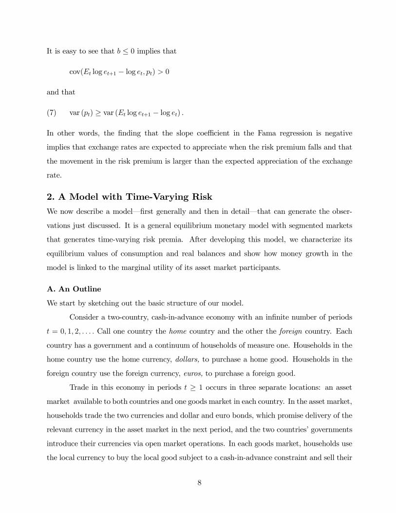
It is easy to see that b ≤ 0 implies that

cov(Et log et+1 − log et, pt) > 0

and that

var (pt) ≥ var (Et log et+1 − log et) .(7)

In other words, the finding that the slope coefficient in the Fama regression is negative

implies that exchange rates are expected to appreciate when the risk premium falls and that

the movement in the risk premium is larger than the expected appreciation of the exchange

rate.

2. A Model with Time-Varying RiskWe now describe a model–first generally and then in detail–that can generate the obser-

vations just discussed. It is a general equilibrium monetary model with segmented markets

that generates time-varying risk premia. After developing this model, we characterize its

equilibrium values of consumption and real balances and show how money growth in the

model is linked to the marginal utility of its asset market participants.

A. An Outline

We start by sketching out the basic structure of our model.

Consider a two-country, cash-in-advance economy with an infinite number of periods

t = 0, 1, 2, . . . . Call one country the home country and the other the foreign country. Each

country has a government and a continuum of households of measure one. Households in the

home country use the home currency, dollars, to purchase a home good. Households in the

foreign country use the foreign currency, euros, to purchase a foreign good.

Trade in this economy in periods t ≥ 1 occurs in three separate locations: an assetmarket available to both countries and one goods market in each country. In the asset market,

households trade the two currencies and dollar and euro bonds, which promise delivery of the

relevant currency in the asset market in the next period, and the two countries’ governments

introduce their currencies via open market operations. In each goods market, households use

the local currency to buy the local good subject to a cash-in-advance constraint and sell their

8

endowment of the local good for local currency. In period 0 there is an initial round of trade

in bonds in the asset market with no trade in goods markets.

Each household must pay a real fixed cost γ for each transfer of cash between the asset

market and a goods market. This fixed cost is constant over time for any specific household,

but it varies across households in both countries according to a distribution F (γ) with density

f(γ).4 Households are indexed by their fixed cost γ. The fixed costs for households in each

country are in units of the local good. We assume F (0) > 0, so that a positive mass of

households has a zero fixed cost.

The only source of uncertainty in this economy is shocks to money growth in the two

countries. The timing within each period t ≥ 1 for a household in the home country is

illustrated in Figure 1. We emphasize the physical separation of the markets by separating

them in the figure. Households in the home country enter the period with the cash P−1y

they obtained from selling their home good endowments in t− 1, where P−1 is the price leveland y is their endowment of their home good. Each government conducts an open market

operation in the asset market, which determines the realizations of money growth rates μ and

μ∗ in the two countries and the current price levels in the two countries P and P ∗.

The household then splits into a worker and a shopper. Each period the worker sells

the household endowment y for cash Py and rejoins the shopper at the end of the period.

The shopper takes the household’s cash P−1y with real value n = P−1y/P and shops for

goods. The shopper can choose to pay the fixed cost γ to transfer an amount of cash Px

with real value x to or from the asset market. This fixed cost is paid in cash obtained in the

asset market. If the shopper pays the fixed cost, then the cash-in-advance constraint is that

consumption c = n+ x; otherwise, this constraint is c = n.

The household also enters the period with bonds that are claims to cash in the asset

market with payoffs contingent on the rates of money growth μ and μ∗ in the current period.

This cash can be either reinvested in the asset market or, if the fixed cost is paid, transferred

to the goods market. With B denoting the current payoff of the state-contingent bonds

purchased in the past, q the price of bonds, andRqB0 the household’s purchases of new

bonds, the asset market constraint is B =RqB0 + P (x + γ) if the fixed cost is paid and

B =RqB0 otherwise. At the beginning of period t+ 1, the household starts with cash Py in

9

the goods market and a portfolio of contingent bonds B0 in the asset market.

In equilibrium, households with a sufficiently low fixed cost pay it and transfer cash

between the goods and asset markets while others do not. We refer to households that pay

the fixed cost as active and those that do not as inactive. Inactive households simply consume

their current real balances.

Throughout, we assume that the shoppers are not allowed to store cash from one

period to the next. This assumption implies that the cash-in-advance constraint holds with

equality and greatly simplifies the analysis. For some models in which agents are allowed to

store cash and end up doing so in equilibrium, see the work of Alvarez, Atkeson, and Edmond

(2003) and Khan and Thomas (2007).

We also assume throughout that in the asset market, households hold their assets in

interest-bearing bonds rather than cash. Note that as long as nominal interest rates are

positive, bonds dominate cash held in the asset market.

B. The Details

Now we flesh out this outline of the economy.

Let Mt denote the stock of dollars in period t, and let μt = Mt/Mt−1 denote the

growth rate of this stock. Similarly, let μ∗t be the growth rate of the stock of euros M∗t . Let

st = (μt, μ∗t ) denote the aggregate event in period t. Then let st = (s1, . . . , st) denote the

state, consisting of the history of aggregate events through period t, and let g(st) denote the

density of the probability distribution over such histories.

In period 0 there is an initial round of trade in bonds in the asset market with no

trade in goods markets. In the asset market in period 0, home households of type γ have

M0 units of home money (dollars), B̄h(γ) units of the home government debt (bonds), and

B̄∗h units of the foreign government debt, which are claims on B̄h(γ) dollars and B̄∗h euros in

the asset market in that period. Likewise, in the asset market in period 0 foreign households

start with M∗0 euro holdings in the foreign goods market, B̄f units of the home government

debt, and B̄∗f(γ) units of the foreign government debt in the asset market.

The home government issues one-period dollar bonds contingent on the aggregate

state st. In period t, given state st, the home government pays off outstanding bonds B(st)

10

in dollars and issues claims to dollars in the next asset market of the form B(st, st+1) at prices

q(st, st+1). Let B̄ denote the stock of outstanding dollar bonds at the beginning of period 0.

The home government budget constraint at st with t ≥ 1 is

B(st) =M(st)−M(st−1) +Zst+1

q(st, st+1)B(st, st+1) dst+1(8)

with M(s0) = M̄ given, and in t = 0, the constraint is B̄ =Rs1q(s1)B(s1) ds1. Likewise, the

foreign government issues euro bonds denoted B∗(st) with bond prices denoted q∗(st, st+1).

The budget constraints for the foreign government are then analogous to the home govern-

ment’s constraints above.

In the asset market in each period and state, home households trade a complete set

of one-period dollar bonds and euro bonds that have payoffs next period contingent on the

aggregate event st+1. Arbitrage between these bonds then implies that

q(st, st+1) = q∗(st, st+1)e(st)/e(st+1),(9)

where e(st) is the exchange rate for one euro in terms of dollars in state st. This arbitrage

relationship implies that the home and foreign bonds are each separately a complete set of

state-contingent assets. Thus, without loss of generality, we can assume that home households

hold only home bonds and foreign households hold only foreign bonds.

Consider now the problem of households of type γ in the home country. Let P (st) denote

the price level in dollars in the home goods market in period t. In each period t ≥ 1, in thegoods market, these households start the period with dollar real balances n(st, γ). They then

choose transfers of real balances between the goods market and the asset market x(st, γ),

an indicator variable z(st, γ) equal to zero if these transfers are zero and one if they are

more than zero, and consumption of the home good c(st, γ) subject to the cash-in-advance

constraint and the transition law,

c(st, γ) = n(st, γ) + x(st, γ)z(st, γ)(10)

n(st+1, γ) =P (st)y

P (st+1),(11)

11

where in (10) in t = 1, the term n(s1, γ) is given by M0/p(s1). In the asset market in t ≥ 1,

home households begin with cash paymentsB(st, γ) on their bonds. They purchase new bonds

and make cash transfers to the goods market subject to the sequence of budget constraints

B(st, γ) =Zst+1

q(st, st+1)B(st, st+1, γ) dst+1 + P (st)

hx(st, γ) + γ

iz(st, γ).(12)

Assume that both consumption c(st, γ) and real bond holdings B(st, γ)/P (st) are uniformly

bounded by some large constants.

In period 0, the asset market constraint for home households is given by

B̄h(γ) + e0B̄∗h =

Zs1q(s1)B(s1, γ) ds1.

In this initial period, home and foreign households trade bonds denominated in the two

currencies and insure themselves against the initial money growth shock s1.

The problem of the home household of type γ is to maximize utility

∞Xt=1

βtZU(c(st, γ))g(st) dst(13)

subject to the constraints (10)—(12). Households in the foreign country solve the analogous

problem, with P ∗(st) denoting the price level in euros in the foreign country goods market.

We require thatRB̄h(γ)f(γ) dγ + B̄f = B̄ and B̄∗h +

RB̄∗f(γ)f(γ) dγ = B̄∗.

Since each transfer of cash between the asset market and the home goods market

consumes γ units of the home good, the total goods cost of carrying out all transfers between

home households and the asset market in t is γRz(st, γ)f(γ) dγ, and likewise for the foreign

households. The resource constraint in the home country is given byZ hc(st, γ) + γz(st, γ)

if(γ) dγ = y(14)

for all t, st, with the analogous constraint in the foreign country. The fixed costs are paid

for with cash obtained in the asset market. Thus, the home country money market—clearing

condition in t ≥ 1 is given byZ ³n(st, γ) +

hx(st, γ) + γ

iz(st, γ)

´f(γ) dγ =M(st)/P (st)(15)

for all st. The money market—clearing condition for the foreign country is analogous. We let

c denote the sequences of functions c(st, γ) and use similar notation for the other variables.

12

An equilibrium in this economy is a collection of bond and goods prices (q, q∗) and (P,

P ∗), together with bond holdings (B,B∗) and allocations for home and foreign households

(c, x, z, n) and (c∗, x∗, z∗, n∗), such that for each transfer cost γ, the bond holdings and the

allocations solve the households’ utility maximization problems, the governments’ budget

constraints hold, and the resource constraints and the money market—clearing conditions are

satisfied.

C. Characterizing Equilibrium

Now, in our model economy, we solve for the equilibrium consumption and real balances of

both active households (those that pay the fixed cost and transfer cash between asset and

goods markets) and inactive households (those that do not). We then characterize the link

between the consumption of active households and asset prices. We focus on households in

the home country; the analysis of households in the foreign country is similar.

Consumption and Real Balances

We start with a household’s decision whether or not to pay the fixed cost in order to transfer

cash between the asset and goods markets. Since households are not allowed to store cash in

the goods market, the cash-in-advance constraint always binds, and any household’s decision

to pay the fixed cost in period t is static. This is because this decision affects only the

household’s current consumption and bond holdings and not the real balances it holds later

in the goods market.

Notice that the constraints (10), (14), and (15) imply that the price level is

P (st) =M(st)/y.(16)

The inflation rate is πt = μt, and real money holdings are n(st, γ) = y/μt. Hence, the

consumption of inactive households is c(st, γ) = y/μt. Let cA(st, γ) denote the consumption

of an active household for a given st and γ.

In this economy, inflation is distorting because it reduces the consumption of any

household that chooses to be inactive. This effect induces some households to use real re-

sources to pay the fixed cost, thereby reducing the total amount of resources available for

consumption. This is the only distortion from inflation in the model. Because of this feature

13

and our assumption that a complete set of nominal claims are traded in the asset market,

the competitive equilibrium allocations and asset prices can be found from the solution to

the following planning problem for the home country, together with that to the analogous

problem for the foreign country.5 Choose z(st, γ) ∈ [0, 1], c(st, γ) ≥ 0, and c(st) ≥ 0 to solve

max∞Xt=1

βtZst

ZγU³c(st, γ)

´f(γ)g(st) dγdst

subject to the resource constraint (14) and this additional constraint:

c(st, γ) = z(st, γ)cA(st, γ) + [1− z(st, γ)]y/μt.(17)

The constraint (17) captures the restriction that the consumption of households that do not

pay the fixed cost is pinned down by their real money balances y/μt. Here the planning weight

for households of type γ is simply the fraction of households of this type.

This planning problem can be decentralized with the appropriate settings of the initial

endowments of home and foreign government debt B̄(γ) and B̄∗(γ). Asset prices are obtained

from the multipliers on the resource constraints above. For simplicity, we have chosen to

focus on the economy in which initial bond holdings are allocated so that all households have

equal Lagrange multipliers on their period 0 budget constraints. The equilibrium allocations

of this economy correspond to those found as the solution to the planning problem with equal

Pareto weights given above. (Economies with different distributions of bond holdings have

equilibrium allocations that correspond to planning problems that have Pareto weights that

depend on γ.)

Notice that the planning problem reduces to a sequence of static problems. We analyze

the consumption pattern first for a fixed choice z to pay the fixed cost and then for the optimal

choice of z.

The first-order condition for an active household’s consumption cA reduces to

βtU 0 ³cA(st, γ)´ g(st) = λ(st),(18)

where λ(st) is the multiplier on the resource constraint. This first-order condition clearly

implies that all households that pay the fixed cost choose the same consumption level, which

means that cA(st, γ) is independent of γ. Since this problem is static, this consumption level

14

depends on only the current money growth shock μt. Hence, we denote this consumption as

cA(μt).

Now, since the solution to the planning problem depends on only current μt and γ,

we drop its dependence on t. It should be clear that the optimal choice of z has a cutoff rule

form: for each shock μ, there is some fixed cost level γ̄(μ) at which the households with γ ≤γ̄(μ) pay this fixed cost and consume cA(μ), and all other households (the inactive ones) do

not pay and consume instead y/μ. For each μ, the planning problem thus reduces to choosing

two numbers, cA(μ) and γ̄(μ), to solve

maxU(cA(μ))F(γ̄(μ))+ U(y/μ)h1− F(γ̄(μ))

isubject to

cA(μ)F(γ̄(μ))+Z γ̄(μ)

0γf(γ) dγ + (y/μ)

h1− F(γ̄(μ))

i= y.(19)

The first-order conditions then can be summarized by (19) and

U(cA(μ))− U(y/μ)− U 0(cA(μ))[cA(μ) + γ̄(μ)− (y/μ)] = 0.(20)

In Appendix B, we show that the solution to these two equations, (19) and (20)–namely,

cA(μ) and γ̄(μ)–is unique. We then can describe the equilibrium consumption and real

balances of active and inactive households in the following proposition:

Proposition 1. The equilibrium consumption of households is given by

c(st, γ) =

⎧⎪⎨⎪⎩ cA (μt) if γ ≤ γ̄(μt)

y/μt otherwise,

where the functions cA (μ) and γ̄(μ) are the solutions to (19) and (20).

Active Household Consumption and Asset Prices

Now we characterize the link between the consumption of active households and asset prices.

In the decentralized economy corresponding to the planning problem, asset prices are

given by the multipliers on the resource constraints for the planning problem. Here, from

(18), these multipliers are equal to the marginal utility of active households.

15

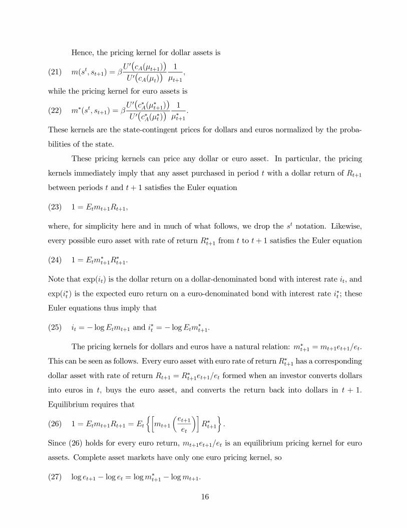
Hence, the pricing kernel for dollar assets is

m(st, st+1) = βU 0(cA(μt+1))U 0(cA(μt))

1

μt+1,(21)

while the pricing kernel for euro assets is

m∗(st, st+1) = βU 0(c∗A(μ∗t+1))U 0(c∗A(μ∗t ))

1

μ∗t+1.(22)

These kernels are the state-contingent prices for dollars and euros normalized by the proba-

bilities of the state.

These pricing kernels can price any dollar or euro asset. In particular, the pricing

kernels immediately imply that any asset purchased in period t with a dollar return of Rt+1

between periods t and t+ 1 satisfies the Euler equation

1 = Etmt+1Rt+1,(23)

where, for simplicity here and in much of what follows, we drop the st notation. Likewise,

every possible euro asset with rate of return R∗t+1 from t to t+ 1 satisfies the Euler equation

1 = Etm∗t+1R

∗t+1.(24)

Note that exp(it) is the dollar return on a dollar-denominated bond with interest rate it, and

exp(i∗t ) is the expected euro return on a euro-denominated bond with interest rate i∗t ; these

Euler equations thus imply that

it = − logEtmt+1 and i∗t = − logEtm∗t+1.(25)

The pricing kernels for dollars and euros have a natural relation: m∗t+1 = mt+1et+1/et.

This can be seen as follows. Every euro asset with euro rate of returnR∗t+1 has a corresponding

dollar asset with rate of return Rt+1 = R∗t+1et+1/et formed when an investor converts dollars

into euros in t, buys the euro asset, and converts the return back into dollars in t + 1.

Equilibrium requires that

1 = Etmt+1Rt+1 = Et

½∙mt+1

µet+1et

¶¸R∗t+1

¾.(26)

Since (26) holds for every euro return, mt+1et+1/et is an equilibrium pricing kernel for euro

assets. Complete asset markets have only one euro pricing kernel, so

log et+1 − log et = logm∗t+1 − logmt+1.(27)

16

Substituting (25) and (27) into our original expression for the risk premium (1) gives that

pt = (Et logm∗t+1 −Et logmt+1)− (logEtm

∗t+1 − logEtmt+1).(28)

Hence, a currency’s risk premium depends on the difference between the expected value of

the log and the log of the expectation of the pricing kernel. Jensen’s inequality implies that

fluctuations in the risk premium are driven by fluctuations in the conditional variability of

the pricing kernel.

Finally, note that given the initial exchange rate e0 and (27) together with the kernels

gives the entire path of the nominal exchange rate et. It is easy to show that the initial

nominal exchange rate is given by

e0 =³B̄ − B̄h

´/B̄∗h,(29)

where B̄h =RB̄h(γ) dF (γ). Clearly, this exchange rate exists and is positive as long as either

B̄h < B̄ and B̄∗h > 0 or B̄h > B̄ and B̄∗h < 0.

D. Linking Money Growth and Active Households’ Marginal Utility

In our model, the active households price assets in the sense that the pricing kernels (21) and

(22) are determined by those households’ marginal utilities. Thus, in order to characterize the

link between money growth and either interest rates or exchange rates, we need to determine

how these marginal utilities respond to changes in money growth, namely, how U 0(cA(μt))

varies with μt.

The Theory

In the simplest monetary models (such as in Lucas 1982), all the agents are active every

period, and changes in money growth have no impact on marginal utilities. Our model

introduces two key innovations to those simple models. One is that here, because of the seg-

mentation of asset markets, changes in money growth do have an impact on the consumption

and, hence, the marginal utility of active households. Our model’s other innovation is that

the size of this impact changes systematically with the size of money growth. As we show,

the change in the size of this impact can be large because the degree of market segmentation

is endogenous. With these two innovations, our model can deliver large and variable currency

risk premia even though the fundamental shocks have constant variance.

17

Mechanically, our model generates variable risk premia that fall as money growth

rises when log cA(μ) is increasing and concave in log μ. To see the link between risk premia

and log cA(μ), define φ(μ) to be the elasticity of the marginal utility of active households

to a change in money growth. With constant relative risk aversion preferences of the form

U(c) = c1−σ/(1− σ), where σ is the degree of relative risk aversion, this elasticity is given by

φ(μ) ≡ −d logU0(cA(μ))

d log μ= σ

d log cA(μ)

d log μ.(30)

Note from (30) that when log cA(μ) is increasing in logμ, φ(μ) > 0. The larger is

φ(μ), the more sensitive is the marginal utility of active households to money growth. Also

note that when log cA(μ) is concave in log μ, φ(μ) decreases in μ; this means the marginal

utility of active households is more sensitive to money growth changes at low levels of money

growth than at high. In this sense, the concavity of log cA(μ) implies that the variability of

the pricing kernel decreases as money growth increases.

We now characterize features of our model’s equilibrium in two propositions. The

proofs of both are in Appendix B.

Proposition 2. As μ increases, more households become active. In particular, γ̄0 (μ) > 0 for

μ > 1, and γ̄0 (1) = 0.

Proposition 3. The log of the consumption of active households cA(μ) is strictly increasing

and strictly concave in log μ around μ = 1. In particular, φ(1) > 0 and φ0(1) < 0.

In Proposition 2, we have shown that more households choose to become active as

money growth and inflation increase. This result is intuitive because as inflation increases,

so does the cost of not participating in the asset market, since the consumption of inactive

households, y/μ, falls as money growth μ increases.

In Proposition 3, we have shown that locally, for low values of money growth at least,

the consumption of active households is increasing and concave in money growth.

A Quadratic Approximation

To capture the nonlinearity of cA(μ) in a tractable way for computing the asset prices im-

plied by our model, we take a second-order approximation to the marginal utility of active

18

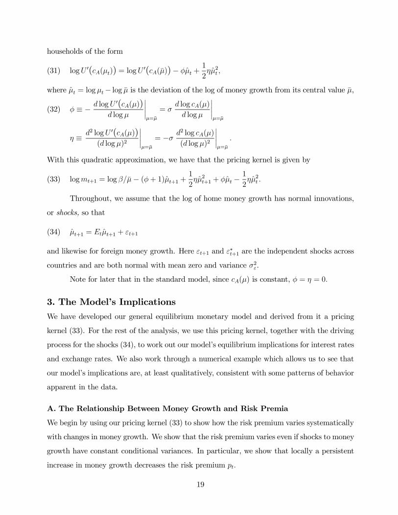
households of the form

logU 0(cA(μt)) = logU 0(cA(μ̄))− φμ̂t +1

2ημ̂2t ,(31)

where μ̂t = log μt− log μ̄ is the deviation of the log of money growth from its central value μ̄,

φ ≡ − d logU 0(cA(μ))d log μ

¯̄̄̄¯μ=μ̄

= σd log cA(μ)

d logμ

¯̄̄̄¯μ=μ̄

(32)

η ≡ d2 logU 0(cA(μ))(d log μ)2

¯̄̄̄¯μ=μ̄

= −σ d2 log cA(μ)

(d log μ)2

¯̄̄̄¯μ=μ̄

.

With this quadratic approximation, we have that the pricing kernel is given by

logmt+1 = log β/μ̄− (φ+ 1)μ̂t+1 +1

2ημ̂2t+1 + φμ̂t −

1

2ημ̂2t .(33)

Throughout, we assume that the log of home money growth has normal innovations,

or shocks, so that

μ̂t+1 = Etμ̂t+1 + εt+1(34)

and likewise for foreign money growth. Here εt+1 and ε∗t+1 are the independent shocks across

countries and are both normal with mean zero and variance σ2ε.

Note for later that in the standard model, since cA(μ) is constant, φ = η = 0.

3. The Model’s ImplicationsWe have developed our general equilibrium monetary model and derived from it a pricing

kernel (33). For the rest of the analysis, we use this pricing kernel, together with the driving

process for the shocks (34), to work out our model’s equilibrium implications for interest rates

and exchange rates. We also work through a numerical example which allows us to see that

our model’s implications are, at least qualitatively, consistent with some patterns of behavior

apparent in the data.

A. The Relationship Between Money Growth and Risk Premia

We begin by using our pricing kernel (33) to show how the risk premium varies systematically

with changes in money growth. We show that the risk premium varies even if shocks to money

growth have constant conditional variances. In particular, we show that locally a persistent

increase in money growth decreases the risk premium pt.

19

Recall that the risk premium can be written in terms of the pricing kernel as in (28):

pt = (logEtmt+1 − Et logmt+1)− (logEtm∗t+1 − Et logm

∗t+1).(35)

Note that if the pricing kernel mt+1 were a conditionally lognormal variable, then, as is well-

known, logEtmt+1 = Et logmt+1 + (1/2)vart(logmt+1). In such a case, the risk premium

pt would equal half the difference of the conditional variances of the log kernels. Given our

quadratic approximation (33), however, the pricing kernel is not conditionally lognormal;

still, a similar relationship between the risk premium and the conditional variance of the

kernel holds.

This relationship is established in the next proposition, the proof of which is in Appen-

dix B. For the resulting risk premium to be well-defined with our quadratic approximation,

we need

ησ2ε < 1,(36)

which we assume for the remainder of our analysis.6

Proposition 4. Under (33), the risk premium is

pt =1

2

1

(1− ησ2ε)

³vart logmt+1 − vart logm∗

t+1

´,(37)

where

vart(logmt+1) = [−(1 + φ) + ηEtμ̂t+1]2σ2ε +

3

4η2σ4ε(38)

and a symmetric formula holds for vart(logm∗t+1).

To see how the risk premium varies with money growth, we calculate the derivative of

the risk premium and evaluate it at μt = μ̄ to get that

dptdμ̂t

= −η(φ+ 1)σ2ε

1− ησ2ε

dEtμ̂t+1dμ̂t

.(39)

Together (36) and (39) imply that the risk premium falls as home money growth rises if

log cA(μ) is concave in log μ, so that η > 0, and if money growth is persistent, so that

dEtμ̂t+1/dμ̂t is positive. Thus, under very simple conditions, we have that the risk premium

decreases as the money growth rate increases.

20

The idea behind that relationship is as follows. Since η is positive, the sensitivity

of marginal utility to fluctuations in money growth decreases as expected money growth

increases. Since money growth is persistent, a high money growth rate in period t leads

households to forecast a higher money growth rate in period t + 1. Thus, a high money

growth rate in period t leads households to predict less variable marginal utility in period

t + 1. Hence, the risk premium in period t decreases as the money growth rate increases in

period t.

B. The Forward Premium Anomaly

We now show that this relationship between money growth and risk premia can lead our model

to generate the forward premium anomaly–the tendency for high interest rate currencies to

appreciate over time. A necessary circumstance is that the persistence of money growth be

within an intermediate range.

From the definition of the risk premium (1), we can write the interest rate differential

as

it − i∗t = Et log et+1 − log et − pt.(40)

As we have seen, a persistent increase in money growth leads the risk premium pt to fall.

When this increase in money growth also leads to an expected exchange rate appreciation

smaller than the fall in the risk premium, the interest rate differential increases, and our

model generates the forward premium anomaly.

The simplest case to study is when exchange rates are random walks, for then an

increase in money growth has no effect on the expected change in the value of the currency.

In this case, because the covariance between the interest rate differential and the expected

change in the exchange rate is zero, the model generates, at least weakly, the forward premium

anomaly.

The more general case is when a persistent increase in money growth leads to an

expected exchange rate appreciation. Recall that in standard models without market seg-

mentation, a persistent increase in money growth leads to the opposite: an expected depreci-

ation. Here we discuss in some detail how our model with asset market segmentation delivers

different implications for the effects of money growth on the exchange rate.

21

To see how an increase in money growth can lead to an expected appreciation of the

nominal exchange rate et in our model, it is helpful to write this expected appreciation as

the sum of the expected appreciation of the real exchange rate and the expected inflation

differential:

Et log et+1 − log et = (Et log vt+1 − log vt) + Et[log(Pt+1/Pt)− log(P ∗t+1/P ∗t )],(41)

where the real exchange rate vt = etP∗t /Pt. In a standard model, an increase in money growth

leads to an expected nominal depreciation because the increased money growth increases

expected inflation but has no effect on real exchange rates. In our model, an increase in

money growth leads to an expected real depreciation that dominates the expected inflation

effect.7

Using our pricing kernels (21) and (22), our expression for changes in exchange rates

(27), and the expression for the home price level together with (16) and its foreign analog,

we can write the right side of (41) in terms of the marginal utility of active households:

Et[logU0(c∗At+1)/U

0(cAt+1)− logU 0(c∗At)/U0(cAt)] + Et[logμt+1 − logμ∗t+1],(42)

where the first bracketed term corresponds to the change in the real exchange rate and the

second to the expected inflation differential. Hence, we can decompose the effect of money

growth changes on the expected change in the nominal exchange rate into two parts: amarket

segmentation effect and an expected inflation effect. The market segmentation effect measures

the impact of an increase in money growth on the expected change in the real exchange rate

through its impact on the marginal utilities in the first bracketed term in (42). This effect

is not present in the standard general equilibrium model, which has no segmentation. The

expected inflation effect, which is present in the standard model, measures the impact of an

increase in money growth on the expected inflation differential in the second bracketed term

in (42).

Now consider the impact of a persistent increase in money growth on the expected

change in the nominal exchange rate. The expected inflation effect is simply

d(Et logμt+1)/d logμt.(43)

22

This effect is larger the more persistent is money growth. In the standard model, this is the

only effect because in that model cA(μ) is constant (and, hence, φ = η = 0). In the standard

model, then, an increase in money growth of one percentage point leads to an expected

nominal depreciation of size d(Et log μt+1)/d log μt.

The size of the market segmentation effect depends on both the degree of market

segmentation and the persistence of money growth. This follows because a persistent increase

in the home money growth rate μt affects both the current real exchange rate

log vt = logU0(c∗A(μ∗t ))/U 0(cA(μt))(44)

and, by increasing the expected money growth rate in t+ 1, the expected real exchange rate

Et log vt+1 = Et logU0(c∗A(μ∗t+1))/U 0(cA(μt+1)).(45)

Using (42), we see that an increase in the home money growth rate μ̂t leads to an expected

change in the real exchange rate of

d

dμ̂t(Et log vt+1 − log vt) = φ

"d(Etμ̂t+1)

dμ̂t− 1

#,(46)

where we have evaluated this derivative at μt = μ̄ and used our quadratic approximation to

the marginal utility of active households.8

As long as money growth is mean-reverting, in that d(Etμ̂t+1)/dμ̂t < 1, an increase

in money growth near the steady state leads to an expected real appreciation. Clearly, the

magnitude of the expected real appreciation depends on both the degree of market segmen-

tation, as measured by φ, and the degree of persistence in money growth, as measured by

d(Etμ̂t+1)/dμ̂t.

Note that the market segmentation effect and the expected inflation effect have oppo-

site signs. If the market segmentation effect dominates, then for values of μt close to μ̄, an

increase in home money growth leads to an expected appreciation of the nominal exchange

rate. This will occur when

dEtμ̂t+1dμ̂t

≤ φ

1 + φ.(47)

Now consider how our model can generate the forward premium anomaly. The defin-

ition of the risk premium (1) implies that

d(it − i∗t )dμ̂t

=d(Et log et+1 − log et)

dμ̂t− dpt

dμ̂t.(48)

23

To get the forward premium anomaly, we need the impact of money growth on the interest

rate differential to have the opposite sign of its impact on expected depreciation. From (39)

we know that an increase in money growth drives down the risk premium. Under (47) this

increase in money growth generates an expected appreciation of the nominal exchange rate.

If the impact of money growth on the risk premium is larger in magnitude than its impact

on the exchange rate, then the forward premium anomaly results.

We summarize this discussion in the following proposition:

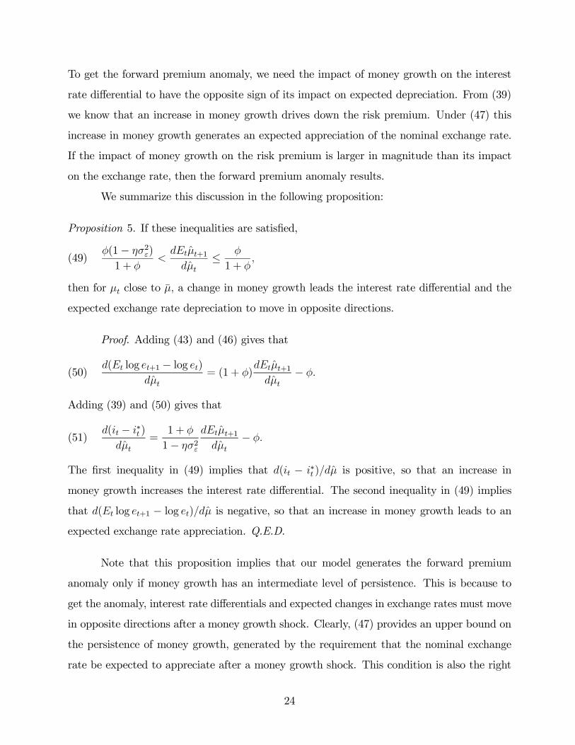
Proposition 5. If these inequalities are satisfied,

φ(1− ησ2ε)

1 + φ<

dEtμ̂t+1dμ̂t

≤ φ

1 + φ,(49)

then for μt close to μ̄, a change in money growth leads the interest rate differential and the

expected exchange rate depreciation to move in opposite directions.

Proof. Adding (43) and (46) gives that

d(Et log et+1 − log et)dμ̂t

= (1 + φ)dEtμ̂t+1dμ̂t

− φ.(50)

Adding (39) and (50) gives that

d(it − i∗t )dμ̂t

=1 + φ

1− ησ2ε

dEtμ̂t+1dμ̂t

− φ.(51)

The first inequality in (49) implies that d(it − i∗t )/dμ̂ is positive, so that an increase in

money growth increases the interest rate differential. The second inequality in (49) implies

that d(Et log et+1 − log et)/dμ̂ is negative, so that an increase in money growth leads to anexpected exchange rate appreciation. Q.E.D.

Note that this proposition implies that our model generates the forward premium

anomaly only if money growth has an intermediate level of persistence. This is because to

get the anomaly, interest rate differentials and expected changes in exchange rates must move

in opposite directions after a money growth shock. Clearly, (47) provides an upper bound on

the persistence of money growth, generated by the requirement that the nominal exchange

rate be expected to appreciate after a money growth shock. This condition is also the right

24

side inequality in (49). The requirement that the movement in the risk premium (39) be

larger than the expected depreciation gives the lower bound on the persistence of money

growth implied by the left side inequality in (49).

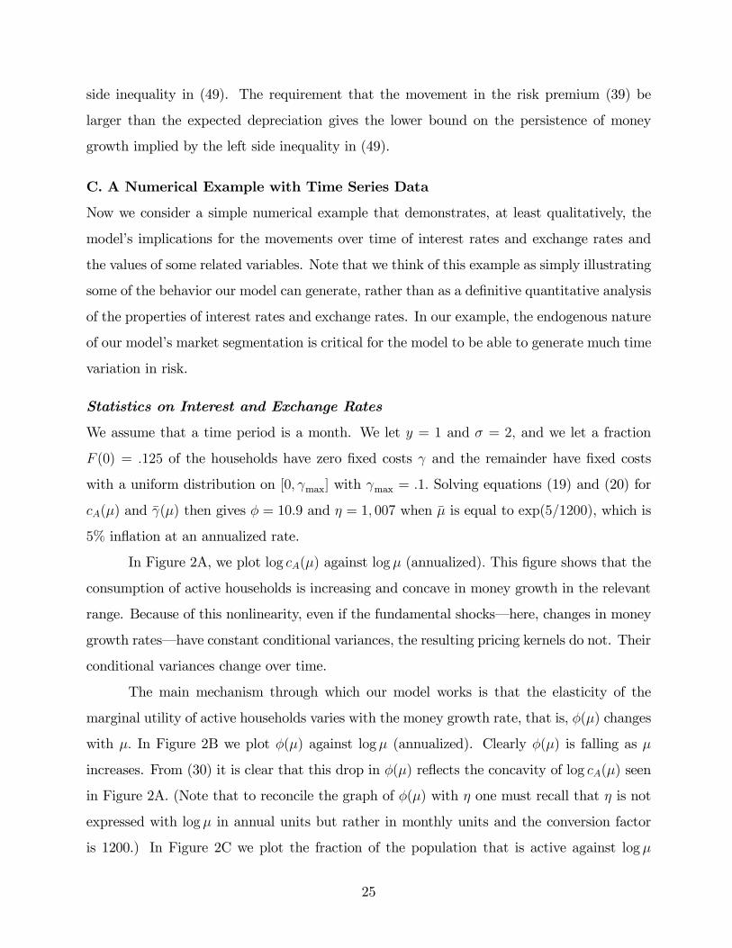
C. A Numerical Example with Time Series Data

Now we consider a simple numerical example that demonstrates, at least qualitatively, the

model’s implications for the movements over time of interest rates and exchange rates and

the values of some related variables. Note that we think of this example as simply illustrating

some of the behavior our model can generate, rather than as a definitive quantitative analysis

of the properties of interest rates and exchange rates. In our example, the endogenous nature

of our model’s market segmentation is critical for the model to be able to generate much time

variation in risk.

Statistics on Interest and Exchange Rates

We assume that a time period is a month. We let y = 1 and σ = 2, and we let a fraction

F (0) = .125 of the households have zero fixed costs γ and the remainder have fixed costs

with a uniform distribution on [0, γmax] with γmax = .1. Solving equations (19) and (20) for

cA(μ) and γ̄(μ) then gives φ = 10.9 and η = 1, 007 when μ̄ is equal to exp(5/1200), which is

5% inflation at an annualized rate.

In Figure 2A, we plot log cA(μ) against log μ (annualized). This figure shows that the

consumption of active households is increasing and concave in money growth in the relevant

range. Because of this nonlinearity, even if the fundamental shocks–here, changes in money

growth rates–have constant conditional variances, the resulting pricing kernels do not. Their

conditional variances change over time.

The main mechanism through which our model works is that the elasticity of the

marginal utility of active households varies with the money growth rate, that is, φ(μ) changes

with μ. In Figure 2B we plot φ(μ) against logμ (annualized). Clearly φ(μ) is falling as μ

increases. From (30) it is clear that this drop in φ(μ) reflects the concavity of log cA(μ) seen

in Figure 2A. (Note that to reconcile the graph of φ(μ) with η one must recall that η is not

expressed with log μ in annual units but rather in monthly units and the conversion factor

is 1200.) In Figure 2C we plot the fraction of the population that is active against logμ

25

(annualized). Clearly, this participation rate rises as μ rises.

Now we use our quadratic approximation to the pricing kernel to illustrate the type of

interest rate and exchange rate behavior that our model can generate. We have constructed

this example so that the exchange rate is a martingale. Hence, interest rates are driven

entirely by movements in the risk premium, and the slope coefficient b in the Fama regression

(5) is zero. We now demonstrate that with these features, our model, in addition to generating

a slope coefficient similar to that in the data, generates some qualitative properties that are

similar to those of the data: interest rate differentials are persistent, and the exchange rate

is an order of magnitude more variable than interest rate differentials.

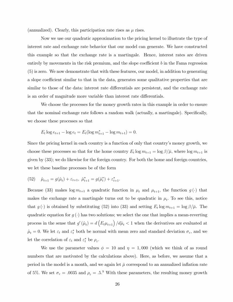
We choose the processes for the money growth rates in this example in order to ensure

that the nominal exchange rate follows a random walk (actually, a martingale). Specifically,

we choose these processes so that

Et log et+1 − log et = Et(logm∗t+1 − logmt+1) = 0.

Since the pricing kernel in each country is a function of only that country’s money growth, we

choose these processes so that for the home country Et logmt+1 = log β/μ̄, where logmt+1 is

given by (33); we do likewise for the foreign country. For both the home and foreign countries,

we let these baseline processes be of the form

μ̂t+1 = g(μ̂t) + εt+1, μ̂∗t+1 = g(μ̂∗t ) + ε∗t+1.(52)

Because (33) makes logmt+1 a quadratic function in μt and μt+1, the function g (·) thatmakes the exchange rate a martingale turns out to be quadratic in μt. To see this, notice

that g (·) is obtained by substituting (52) into (33) and setting Et logmt+1 = log β/μ̄. The

quadratic equation for g (·) has two solutions; we select the one that implies a mean-revertingprocess in the sense that g0 (μ̂t) = d

³Etμt+1

´/dμ̂t < 1 when the derivatives are evaluated at

μ̂t = 0. We let εt and ε∗t both be normal with mean zero and standard deviation σε, and we

let the correlation of εt and ε∗t be ρε.

We use the parameter values φ = 10 and η = 1, 000 (which we think of as round

numbers that are motivated by the calculations above). Here, as before, we assume that a

period in the model is a month, and we again let μ̄ correspond to an annualized inflation rate

of 5%. We set σε = .0035 and ρε = .5.9 With these parameters, the resulting money growth

26

process of the form (52) is similar to that of an AR(1) process with an autocorrelation of .90.

To demonstrate this similarity, in Figure 3 we plot 245 realizations of our baseline money

growth process (52) and this AR(1) process based on the same driving shocks εt.

Now return to Table 1. There we have examined some properties of interest rates and

exchange rates in the data; here we compare to those data the properties implied by this

example. The model’s statistics for this example are reported for the slope coefficient b = 0.

These model statistics are computed as the means over 100,000 draws of 245 periods each.

The statistics in the data, recall, are averages of the statistics for seven European countries

presented by Backus, Foresi, and Telmer (2001), each of which has 245 months of data.

The table shows that in both the data and the model, interest rate differentials do

vary, but not as much as changes in the exchange rate. Interest rate differentials are roughly

one-third as variable in the model as in the data. But in both the data and the model, changes

in the exchange rate have virtually no autocorrelation, whereas interest rate differentials have

a high autocorrelation. At a qualitative level, therefore, our model successfully reproduces

these features of the data.

Other Time Series Statistics

Our model also has implications for the disconnect between aggregate consumption and real

exchange rates. In this example, aggregate consumption is essentially constant, but real

exchange rates are quite variable; hence, real exchange rates are essentially disconnected

from fluctuations in aggregate consumption. In this sense, our model is consistent with the

Backus-Smith puzzle (Backus and Smith 1993).

As discussed in our 2002 work, another feature of the data is that nominal and real

exchange rates have similar volatilities. From (46) and (50), we see that when φ is large, our

model will reproduce that observation. For instance, in our numerical example, the standard

deviation of changes in the real exchange rate is about 93% the size of the standard deviation

of changes in the nominal exchange rate.

We also considered an alternative numerical example with the money growth process

of the form (52) in which the function g(·) is chosen so that the slope coefficient b in theFama regression is equal to −1 in population. The statistics for this numerical example, also

27

reported in Table 1, are nearly identical to those of the earlier example.

The Role of Endogenous Segmentation

Now we show that allowing for endogenous segmentation in our model is a critical feature for

it to be able to generate substantial amounts of time variation in risk.

In our model, even if segmentation were exogenous, so that the fraction of households

that are active were fixed, our model still could generate time-varying risk. This is because the

result in Proposition 3 does not depend on the finding of Proposition 2, that more households

pay the fixed cost when money growth increases. Hence, log cA(μ) is concave, at least locally,

even if the fraction of households that pay the fixed cost does not change with μ. Thus, the

same result would hold if segmentation were exogenous.

If segmentation were exogenous, however, the model could not generate much time

variation in risk. To see that, suppose that a fraction F (0) of households have zero fixed costs

and, hence, are active and that the rest of the households are inactive. For this exogenous

segmentation model, it is easy to show that

φ = σ1− F (0)

μ̄− [1− F (0)]and η =

μ̄

μ̄− [1− F (0)]φ.(53)

Thus, for example, with σ = 2 and μ̄ = (1.05)1/12, to have φ = 10, we need F (0) = 1/6 and,

hence, η = 60. This value of η is an order of magnitude smaller than the value generated

by our endogenous segmentation model. As we show in Table 1 in the row labeled With

Exogenous Segmentation, when we simulate interest rates and exchange rates with these new

values of φ and η, choosing money growth to ensure that exchange rates follow a random

walk, we find that interest rates barely fluctuate. In particular, the standard deviation of the

interest rate differential from the model is one one-hundredth of that in the data.

Note, finally, that with F (0) = 1, so that all households are always active, the model

reduces to the standard constant velocity cash-in-advance model with no time variation in

risk.

D. Long-Run Averages

So far we have focused on the implications of our model for fluctuations over time in the

interest rate differential and the exchange rate for a single pair of currencies. We have

28

shown that our model can generate the forward premium anomaly, or the observation that

high interest rate currencies tend to appreciate over time. The data on long-run averages of

interest rate differentials and exchange rate changes in a cross section of currencies tend to

show the opposite pattern as the time series data: currencies that have high interest rates on

average tend to depreciate on average. (See, for example, Backus, Foresi, and Telmer 2001.)

Here we document that and then show that our model is qualitatively consistent with this

feature of the data as well.

To document this feature, we use monthly data on 14 countries kindly provided by

Ravi Bansal and Magnus Dahlquist. We use these data for the period from January 1976

to March 1998 to construct average one-month interest rate differentials between the U.S.

rate and each of the other countries’ rate as well as corresponding averages of exchange rate

changes over the period.

Figure 4A displays a scatterplot of the resulting values. It shows a clear positive

relationship between the averages, with a slope close to 1.

Our model is consistent with this cross section observation. To see that, suppose we

have a collection of countries with differing permanent components of their money growth

rates μ̄i that, in annualized terms, vary between 1% and 12% per year. For each of these

countries, we use values for the fixed costs and the risk aversion parameter from our numerical

examples to compute the implied values of φi and ηi. We then construct money growth

processes, indexed by gi(μt) as before, so that for each country i, Et logmit+1 = log β/μ̄i,

where logmit+1 is the pricing kernel for country i.We then simulate 100,000 samples of length

245 for these countries and compute the average interest rate differential and exchange rate

change relative to our baseline country, which has the permanent component of its money

growth equal to 5% on an annualized basis.

In Figure 4B we plot the resulting average exchange rate changes against the average

interest rate differentials. Comparing Figures 4A and 4B, we see that our model is consistent

with the cross section observation that over the long run, currencies of countries that have

high interest rates on average tend to depreciate on average.

Of course, the standard model with no segmentation is consistent with this cross

section data as well. Unlike the standard model, however, our model can generate these

29

long-run averages while at the same time generating the time series patterns of interest and

exchange rates that underlie the forward premium anomaly.

4. ConclusionWe have constructed a simple, general equilibrium monetary model with endogenously seg-

mented asset markets and have shown that this sort of friction may be a critical feature of

a complete model of interest rates and exchange rates. The fundamental challenge behind

this exercise has been to develop a model in which exchange rates roughly follow a random

walk (so that expected changes in exchange rates are roughly constant) while interest rate

differentials are highly variable and persistent. In such a model, by definition, movements in

interest rate differentials are movements in risk. Our main contribution here is to propose a

mechanism through which that risk changes because of changes in monetary policy.

30

Appendix A: An Extension with Trade in Goods

In the work above, we have kept the model simple by abstracting from the possibility of trade

in goods. Here we sketch out a version of the model with trade in goods that works similarly

to the original model. Essentially we take the models of Helpman and Razin (1982) and Lucas

(1982) and extend them to have fixed costs of accessing asset markets. We demonstrate that

this extended model leads to results similar to those in the simple model. (Note that in

our economy we assume that goods are purchased in the sellers’ currency. An alternative

assumption is that goods are purchased in the buyers’ currency. For a discussion of the role

of these alternative assumptions, see Helpman and Razin 1984.)

In this extended model, let there be two goods h and f, referred to as home and foreign

goods. Households in the home country have endowments yh and yf of these goods, while

households in the foreign country have endowments y∗h and y∗f . Home country households have

an additively separable period utility function over these goods

αU(ch) + (1− α)U(cf),

where α ∈ (0, 1] and (ch, cf) denotes the consumption of the home and foreign goods by thehome households. Foreign households have a similar period utility function

αU(c∗f) + (1− α)U(c∗h),

where (c∗h, c∗f) denotes the consumption of the home and foreign goods. When α ≥ 1/2,

preferences exhibit a type of home bias: home country households consume relatively more

home goods, and foreign households, relatively more foreign goods.

As in Helpman and Razin (1982) and Lucas (1982), home goods must be purchased

with home currency and foreign goods with foreign currency. Specifically, households in

each country have one cash-in-advance constraint for purchases of home goods and one for

purchases of foreign goods. Home households have a fixed cost γ that applies to each transfer

of home currency between the home goods market and the asset market, and a separate fixed

cost γ∗ that applies to each transfer of foreign currency between the foreign goods market

and the asset market. Home households are indexed by (γ, γ∗) , which we assume have joint

distribution given by F (γ)F ∗(γ∗). Foreign households are indexed by a symmetric distribution

31

of costs: F (γ) for transfers between foreign goods markets and the asset market and F ∗(γ∗)

for transfers between home goods markets and the asset market.

In the model, households now have more options of participation in the goods and asset

markets. They can transfer only home currency, only foreign currency, both currencies, or

none at all. For these different patterns of transfer, the home households will pay γ, γ∗, γ+γ∗,

and 0, respectively, while the foreign households will pay γ∗, γ, γ∗ + γ, and 0, respectively.

It can be shown that the equilibrium allocations of home goods solve the following planning

problem that is the obvious generalization of the one in the simpler model without trade in

goods:

maxchA,c

∗hA.γ̄h,γ̄

∗h

αU(chA)F (γ̄h) + αU(yh/μ)[1− F (γ̄h)]

+ (1− α)U(c∗hA)F∗(γ̄∗h) + (1− α)U(y∗h/μ)[1− F ∗(γ̄∗h)]

subject to

chA F (γ̄h) +Z γ̄h

0γf(γ)dγ + [1− F (γ̄h)]yh/μ

+c∗hA F ∗(γ̄∗h) +Z γ̄∗h

0γf ∗(γ)dγ + [1− F ∗(γ̄∗h)]y

∗h/μ = yh + y∗h.

Here we denote the consumption of home goods by the home and foreign households by

chA and c∗hA. We also denote the cutoff values for transferring home currency to the home

goods market by the home and foreign households by γ̄h and γ̄∗h. The equilibrium allocations

of foreign goods solve a similar problem.

The solution to the problem for home goods is similar to the simpler problem in

which goods are not tradable. The link between money injections and households’ marginal

utilities is also similar. The key distinctions between the model with and without tradable

goods are as follows. Here all active households equate their marginal utilities; hence, the

consumption of home goods of home and foreign active households moves together. If a home

household does not make a transfer of home currency, then the home consumption of home

goods is ch = yh/μ. If a foreign household does not make a transfer of home currency, then

its consumption of the home good is c∗h = y∗h/μ. Hence, the value of making a transfer of

home currency for a home household differs from that of making one for a foreign household.

32

Likewise, the cost of making such a transfer is drawn from F (γ) for a home household and

from F ∗(γ∗) for a foreign household. Because of these differences in the value and costs

of making transfers, in general, the home households have a cutoff function for transfers of

home currency γ̄h(μ) which differs from the cutoff that foreign households have for transfers

of home currency γ̄∗h(μ). A similar distinction holds with respect to foreign currency transfers.

Consider now a utility function of the form U(c) = c1−σ/ (1− σ) . It is easy to show

that the optimal allocations {chA (μ) , c∗hA (μ) , γ̄h (μ) , γ̄∗h (μ)} are increasing functions of

μ and that the consumption of home goods of the home and foreign active households are

proportional, c∗hA (μ) = ω chA (μ), where ω = [(1− α) /α]1σ .

Next we present a proposition in which the determination of the active households’

consumption and cutoff function is identical to that in the model without tradable goods.

Proposition 8. Assume that endowments satisfy

y∗h/yh = ω(54)

and that the upper bound of the support for γ, denoted γmax, satisfies F∗ (ωγmax) = 1. Then

γ̄h(μ) and γ̄∗h(μ) satisfy γ̄∗h (μ) = ω γ̄h(μ), and the values of chA (μ) and γ̄h (μ) are identical

to those in an economy with no tradable goods, an aggregate endowment of yh + y∗h, and a

distribution of costs given by

F̃ (γ) =F (γ) + ωF ∗(ωγ)

1 + ω.

The proof of this proposition follows from verifying that the candidate solution satisfies

the first-order conditions of the problem stated above. The assumption (54) includes the case

of completely symmetric countries, α = 1/2 and yh = y∗h, but it is more general. In particular,

this assumption allows for a type of home bias preference of α ≥ 1/2 and specialization inthe endowments in the sense of yh > y∗h. The home bias implies that ch ≥ cf at μ = μ∗. This

assumption implies that for μ = 1, exports are zero, since ch = yh. For μ > 1, however, there

typically will be trade in equilibrium, provided that F and F ∗ differ.

When assumption (54) is not satisfied, γ̄h and γ̄∗h move together with μ, but they are

not necessarily proportional; hence, the expression of chA(μ) does not reduce exactly to that

33

of the model with no tradable goods. Nevertheless, the expressions for chA and γ̄h are similar

to those in that model.

To see why, consider the extreme case in which y∗h = 0, so that the foreign country

has no endowment of the home good. In this case, under appropriate conditions, all foreign

households engage in transfers of home currency, so that γ̄∗h (μ) = γ∗max. The resulting ex-

pressions for chA (μ) and γ̄h (μ) correspond to those for the model with no tradable goods,

the cost functions F̃ (γ) = [F (γ) + ω]/ (1 + ω) and F̃ (0) = ω / (1 + ω), the consumption of

inactive home households yh/μ, and the aggregate endowment [yh − R γ∗dF ∗ (γ∗)] / (1 + ω) .

Appendix B: Some Proofs

Proof of Unique Solution (Requirement for Proposition 1)

Here we show that equations (19) and (20) have at most one solution for any given μ.

To see this result, solve for γ̄ as a function of cA from (20) and suppress explicit

dependence of μ to get

γ̄(cA) =U(cA)− U(y/μ)

U 0(cA)− [cA − (y/μ)] .

Note that

dγ̄(cA)

dcA= − U 00(cA)

[U 0(cA)]2[U(cA)− U(y/μ)].(55)

Use (20) to see that dγ̄(cA)/dcA is positive when cA + γ̄ − (y/μ) > 0 and negative when

cA + γ̄ − (y/μ) < 0. Substituting γ̄(cA) into (19) and differentiating the left side of the

resulting expression with respect to cA gives

F(γ̄(cA))+ [cA + γ̄(cA)− (y/μ)] dγ̄(cA)dcA

.(56)

Using (55), we see that (56) is strictly positive; hence, the equations have at most one solution.

Q.E.D.

Proof of Proposition 2

Differentiating equations (19) and (20) with respect to μ and solving for γ̄0 gives that

γ̄0 (μ) =[U 0 (y/u)− U 0 (cA)] (y/μ)− U 00 (cA) [cA + γ̄ − (y/μ)]1−F

Fy/μ2

U 0 (cA)− U 00 (cA) [cA + γ̄ − (y/μ)]f/F ,

34

where to simplify we have omitted the arguments in the functions F, f, cA, and γ̄. Note that

cA (1) = y and γ̄ (1) = 0. Also note that (19) implies that if μ > 1, then cA + γ̄ − (y/μ) > 0.To derive this result, rewrite (19) as

cA(μ) +

R γ̄(μ)0 γf(γ) dγ

F(γ̄(μ))− y/μ =

y − y/μ

F(γ̄(μ)),(57)

use the inequality γ̄(μ) ≥³R γ̄(μ)0 γf(γ) dγ

´/F (γ̄(μ)), and note that the right side of (57) is

strictly positive for μ > 1. It follows from this result and (20) that U 0 (y/μ)−U 0 (cA) > 0 for

μ > 1. Finally, since U is strictly concave, U 00 (cA) < 0; thus, γ̄0 > 0 for μ > 1. Using similar

results for μ = 1, we get that γ0 (1) = 0. Q.E.D.

Proof of Proposition 3

We first show that φ (1) = σ[1 − F (0)]/F (0), which is positive when F (0) > 0. To see this,

differentiate (19) with respect to μ and γ̄, and use, from Proposition 2, that γ̄0 (1) = γ̄ (1) = 0

in order to get that

c0A (1) = y1− F (0)

F (0).

Using this expression for c0A(1) and using cA (1) = y in φ(1) = σc0A(1)/cA(1) gives our intended

result.

We next show that φ0(1) = −φ(1)/F (0), which is negative because φ(1) > 0 and

F (0) > 0. To see this, first differentiate (30) to get that

φ0 (1) = σ

⎡⎣c00A (1)cA (1)

+c0A (1)cA (1)

−Ãc0A (1)cA (1)

!2⎤⎦ .(58)

Second, differentiate (19) with respect to μ and γ̄, and use the result at μ = 1, γ̄0 (μ) =

γ̄ (μ) = 0, and cA (μ) + γ̄ (μ)− y/μ = 0 to get that

c00A (1) = −2y1− F (0)

F (0).

Using these expressions for c0A and c00A in (58) produces the desired result. Q.E.D.

Proof of Proposition 4

To prove Proposition 4, we derive two equations, (37) and (38).

35

To derive (37), start with (35), the risk premium defined in terms of the pricing kernels.

Compute Et logmt+1 from (33). To compute logEtmt+1, we must compute

logEt expµh−(φ+ 1) + ηEtμ̂t+1

iεt+1 +

η

2ε2t+1

¶.

To do that, use the result that if x is normally distributed with mean zero and variance

σ2 and satisfies 1− 2bσ2 > 0, then

E exp³ax+ bx2

´= exp

Ã1

2

a2σ2

(1− 2bσ2)!µ

1

1− 2σ2b¶1/2

.(59)

To derive (59), note that

E exp³ax+ bx2

´=

1

σ√2π

Zexp

³ax+ bx2

´exp

Ã− x2

2σ2

!dx =

1

σ√2π

Zexp

µ1

2σ2

h2σ2ax+

³2σ2b− 1

´x2i¶

dx =

1

σ√2π

Zexp

Ã1

2σ2

"−³1− 2σ2b

´x2 + 2σ2ax−

Ãσ4a2

1− 2σ2b!+

Ãσ4a2

1− 2σ2b!#!

dx =

exp

Ã1

2

a2σ2

(1− 2bσ2)!

1

σ√2π

Zexp

⎛⎝− 1

2σ2

"³1− 2σ2b

´1/2x− σ2a

(1− 2σ2b)1/2#2⎞⎠ dx =

exp

Ã1

2

a2σ2

(1− 2bσ2)!

1

σ√2π

Zexp

⎛⎝−(1− 2σ2b)2σ2

"x− σ2a

(1− 2σ2b)#2⎞⎠ dx.

which equals (59).

We can derive (38) using (33) together with the standard results that Etε4t+1 = 3σ4ε

and Etε3t+1 = 0. Q.E.D.

36

Notes

1Technically, pt is simply the log of the excess return on foreign currency bonds. In

general, this excess return could arise for many reasons, including differences in taxes, liquidity

services, or transaction costs across bonds. We take the view here that fluctuations in this

excess return are driven primarily by risk; hence, we refer to the excess return as the risk

premium.

2The forward premium anomaly can also be stated in terms of forward exchange rates.

The forward exchange rate ft is the price specified in a contract in period t in which the

buyer has the obligation to transfer ft dollars in t+1 in exchange for one euro. The forward

premium is then the forward rate relative to the spot rate ft/et. Arbitrage implies that

log ft − log et = it − i∗t . Thus, (3) can be restated as cov(log ft − log et, log et+1 − log et) < 0.The forward premium and the expected change in exchange rates, therefore, tend to move in

opposite directions. This observation contradicts the hypothesis that the forward rate is a

good predictor of the future exchange rate.

3To see that (4) implies (6), use (1) to rewrite (4) as var(it − i∗t ) + cov(it − i∗t , pt) ≤ 0or

var (it − i∗t ) ≤ −cov (it − i∗t , pt) = −corr (it − i∗t , pt) std (it − i∗t ) std (pt) .

Then, as does Fama (1984), divide by std(it − i∗t ), and use the fact that a correlation is less

than or equal to one in absolute value.

4It is easy to see that if we replace the assumption that each household draws its fixed

cost once with the assumption that each household takes an i.i.d. draw of its fixed cost each

period, the analysis is identical.

5Recall our assumptions that a complete set of nominal claims are traded in the asset

market and that agents face a fixed cost of transferring cash between the asset market and

the goods market. These assumptions imply that we do not have a complete set of con-

tingent claims to consumption. Because of the fixed cost, households choose to bear some

consumption risk endogenously.

37

6This condition ensures that Etmt+1 exists. In Appendix B, in the proof of Proposition

4, we need the generalization of this condition: 1− 2bσ2 > 0. In the proof, when we computeZexp(−(1− 2bσ2)x2) dx,

we need this condition to have this integral well-defined.

7Note that in both our segmented market model and the standard model, when today’s

money growth rate increases, today’s exchange rate depreciates. In the segmented market

model, this initial depreciation is so large that it leads to overshooting, in that after the

impact period, the exchange rate appreciates. In the standard model, this initial depreciation

is small, and hence, it leads to undershooting, in that after the impact period, the exchange

continues to depreciate.

8Doing so gives that the expected depreciation of the real exchange rate is given by

Et log vt+1 − log vt =

−φEt(μ̂∗t+1 − μ̂t+1) +

1

2ηEt(μ̂

∗2t+1 − μ̂2t+1) + φ(μ̂∗t − μ̂t)−

1

2η(μ̂∗2t − μ̂2t ).

9See Brandt, Cochrane, and Santa-Clara (2006) for a discussion of the correlation of

home and foreign pricing kernels needed to explain the data.

38

References

Allen, Franklin, and Douglas Gale. 1994. Limited market participation and volatility

of asset prices. American Economic Review 84 (4, September): 933—55.

Alvarez, Fernando, and Andrew Atkeson. 1997. Money and exchange rates in the

Grossman-Weiss-Rotemberg model. Journal of Monetary Economics 40 (3, December): 619—

40.

Alvarez, Fernando, Andrew Atkeson, and Chris Edmond. 2003. On the sluggish re-

sponse of prices to money in an inventory-theoretic model of money demand. NBERWorking

Paper 10016.

Alvarez, Fernando, Andrew Atkeson, and Patrick J. Kehoe. 2002. Money, interest

rates, and exchange rates with endogenously segmented markets. Journal of Political Econ-

omy 110 (1, February): 73—112.

Alvarez, Fernando, and Urban J. Jermann. 2001. Quantitative asset pricing impli-

cations of endogenous solvency constraints. Review of Financial Studies 14 (4, Winter):

1117—51.

Backus, David K., Silverio Foresi, and Chris I. Telmer. 1995. Interpreting the forward

premium anomaly. Canadian Journal of Economics 28 (Special issue, November): S108—19.

Backus, David K., Silverio Foresi, and Chris I. Telmer. 2001. Affine term structure

models and the forward premium anomaly. Journal of Finance 56 (1, February): 279—304.

Backus, David K., Allan W. Gregory, and Chris I. Telmer. 1993. Accounting for

forward rates in markets for foreign currency. Journal of Finance 48 (5, December): 1887—

1908.

Backus, David K., and Gregor W. Smith. 1993. Consumption and real exchange rates

in dynamic economies with non-traded goods. Journal of International Economics 35 (3-4,

November): 297—316.

Bansal, Ravi, and Magnus Dahlquist. 2000. The forward premium puzzle: Different

tales from developed and emerging economies. Journal of International Economics 51 (1,

June): 115—44.

Bansal, Ravi, A. Ronald Gallant, Robert Hussey, and George Tauchen. 1995. Non-

parametric estimation of structural models for high-frequency currency market data. Journal

39

of Econometrics 66 (1—2, March—April): 251—87.

Bansal, Ravi and Ivan Shaliastovich. 2007. Risk and return in bond, currency, and

equity markets. Manuscript, Duke University.

Basak, Suleyman, and Domenico Cuoco. 1998. An equilibrium model with restricted

stock market participation. Review of Financial Studies 11 (2, Summer): 309—41.

Baumol, William J. 1952. The transactions demand for cash: An inventory theoretic

approach. Quarterly Journal of Economics 66 (4, November): 545—56.

Bekaert, Geert. 1996. The time variation of risk and return in foreign exchange

markets: A general equilibrium perspective. Review of Financial Studies 9 (2, Summer):

427—70.

Brandt, Michael W., John H. Cochrane, and Pedro Santa-Clara. 2006. International

risk sharing is better than you think, or exchange rates are too smooth. Journal of Monetary

Economics 53, (4, May): 671—98.

Brav, Alon, George M. Constantinides, and Christopher C. Geczy. 2002. Asset pricing

with heterogeneous consumers and limited participation: Empirical evidence. Journal of

Political Economy 110 (4, August): 793—824.

Campbell, John Y., and John H. Cochrane. 1999. By force of habit: A consumption-

based explanation of aggregate stock market behavior. Journal of Political Economy 107 (2,

April): 205—51.

Canova, Fabio, and Jane Marrinan. 1993. Profits, risk, and uncertainty in foreign

exchange markets. Journal of Monetary Economics 32 (2, November): 259—86.

Cochrane, John H. 2001. Asset Pricing. Princeton, N.J.: Princeton University Press.

Engel, Charles. 1996. The forward discount anomaly and the risk premium: A survey

of recent evidence. Journal of Empirical Finance 3 (2, June): 123—92.

Fama, Eugene F. 1984. Forward and spot exchange rates. Journal of Monetary Eco-

nomics 14 (3, November): 319—38.

Fuerst, Timothy S. 1992. Liquidity, loanable funds, and real activity. Journal of

Monetary Economics 29 (1, February): 3—24.

Grilli, Vittorio, and Nouriel Roubini. 1992. Liquidity and exchange rates. Journal of

International Economics 32 (3—4, May): 339—52.

40

Hansen, Lars Peter, and Ravi Jagannathan. 1991. Implications of security market

data for models of dynamic economies. Journal of Political Economy 99 (2, April): 225—62.

Helpman, Elhanan, and Assaf Razin. 1982. Dynamics of a floating exchange rate

regime. Journal of Political Economy 90 (4, August): 728—54.

Helpman, Elhanan, and Assaf Razin. 1984. The role of saving and investment in

exchange rate determination under alternative monetary mechanisms. Journal of Monetary

Economics 13 (3, May): 307—25.

Hodrick, Robert J. 1987. The Empirical Evidence on the Efficiency of Forward and

Futures Foreign Exchange Markets. Chur, Switz.: Harwood Academic Publishers.

Hodrick, Robert J. 1989. Risk, uncertainty, and exchange rates. Journal of Monetary

Economics 23 (3, May): 433—59.

Khan, Aubhik, and Julia K. Thomas. 2007. Inflation and interest rates with endoge-

nous market segmentation. Working Paper 07-1, Federal Reserve Bank of Philadelphia.

Lucas, Robert E., Jr. 1982. Interest rates and currency prices in a two-country world.

Journal of Monetary Economics 10 (3, November): 335—59.

Lucas, Robert E., Jr. 1990. Liquidity and interest rates. Journal of Economic Theory

50 (2, April): 237—64.

Lustig, Hanno, and Stijn Van Nieuwerburgh. 2005. Quantitative asset pricing impli-

cations of housing collateral constraints. Manuscript, University of California, Los Angeles.

Lustig, Hanno, and Adrien Verdelhan. 2007. The cross section of foreign currency risk

premia and consumption growth risk. American Economic Review 97 (1, March): 89—117.

Mankiw, N. Gregory, and Stephen P. Zeldes. 1991. The consumption of stockholders

and nonstockholders. Journal of Financial Economics 29 (1, March): 97—112.

Mehra, Rajnish, and Edward C. Prescott. 1985. The equity premium: A puzzle.

Journal of Monetary Economics 15 (2, March): 145—61.

Obstfeld, Maurice, and Kenneth Rogoff. 1996. Foundations of International Macro-

economics. Cambridge, Mass.: MIT Press.

Obstfeld, Maurice, and Kenneth Rogoff. 2001. Risk and exchange rates. Manuscript,

University of California, Berkeley.

41

Rotemberg, Julio J. 1985. Money and the terms of trade. Journal of International

Economics 19 (1—2, August): 141—60.

Schlagenhauf, Don E., and Jeffrey M. Wrase. 1995. Liquidity and real activity in a

simple open economy model. Journal of Monetary Economics 35 (3, August): 431—61.

Tobin, James. 1956. The interest-elasticity of transactions demand for cash. Review

of Economics and Statistics 38 (3, August): 241—47.

Vissing-Jorgensen, Annette. 2002. Limited asset market participation and the elas-

ticity of intertemporal substitution. Journal of Political Economy 110 (4, August): 825—53.

42

Figure 1 Timing in the Two Markets for a Household in the Home Country

If transfer x, pay fixed cost γ.

Cash-in-Advance Constraint Consumption: c = n + x if cash transferred. c = n if no transfer.

Real balances n = P−1y /P

Shopper

Endowment sold for cash Py

Asset Market Constraint Bonds: B = Ç qB′ + P(x+γ) if cash transferred.B = Ç qB′ if no transfer.

Worker

Starting cash P−1y

Ending cash Py

Starting bonds B

Endingbonds B′

Asset Market

Goods Market

Rate of money growth μ observed

.00

.01

.02

.03

.04

.05

.06

.07

.08

0 1 2 3 4 5 6 7 8 9 10 11 12 13 14 15 16 17 18 19 20

Figure 2A How the Log of the Consumption of Active Households Is Related to the Log of Money Growth

log μ (annualized)

log

c A

0

2

4

6

8

10

12

14

16

0 1 2 3 4 5 6 7 8 9 10 11 12 13 14 15 16 17 18 19 20

Figure 2B How the Elasticity of Marginal Utility φ(μ) Is Related to the Log of Money Growth

log μ (annualized)

φ(μ)

0%

10%

20%

0 1 2 3 4 5 6 7 8 9 10 11 12 13 14 15 16 17 18 19 20

Figure 2C How the Fraction of Active Agents Is Related to the Log of Money Growth

log μ (annualized)

perc

ent a

ctiv

e

-.02

-.01

.00

.01

.02

0 25 50 75 100 125 150 175 200 225

Figure 3 Realizations of Money Growth from Our Baseline Process and an AR(1) Process

Period

Baseline Process

AR(1) Process

Figure 4 The Cross Section Average Interest Rate Differentials and Exchange Rate Changes

Figure 4A In the Data Average One-Month Interest Rate Differential (U.S. Less Other Country) vs. Average One-Month Change in Exchange Rate (with U.S. Dollar) January 1976–March 1998, for 14 Countries*

-6

-4

-2

0

2

4

6

8

10

-6 -4 -2 0 2 4 6 8 10 12

Interest Rate Differential

Exch

ange

Rat

e C

hang

e

45o line

*The countries are Austria, Belgium, Canada, Denmark, England, France, Germany, Italy, Japan, the Netherlands, Portugal, Spain, Sweden, and Switzerland. Sources: Data studied in Ravi Bansal and Magnus Dahlquist 2000

Figure 4B In the Model Average One-Month Interest Rate Differential (Home Less Foreign Country) vs. Average One-Month Change in Exchange Rate (with Home Currency) Over 245 Months**

-6

-4

-2

0

2

4

6

8

10

-6 -4 -2 0 2 4 6 8 10 12

Interest Rate Differential

Exch

ange

Rat

e C

hang

e

45o line

**For the home country, we used the baseline process for money with the permanent component of money growth μ equal to 5% at an annual basis. We then constructed 29 foreign countries with the same process for money except that μ varies from 1% to 12% in .5% increments. We then computed the average one-month interest rate differential and average one-month depreciation rate over 100,000 simulations of length 245.

Table 1 Interest and Exchange Rates in the Data and the Model

Monthly

Standard Deviations Autocorrelations Source of Statistic

Interest Rate Differentials

Exchange Rate Changes

Interest Rate Differentials

Exchange Rate Changes

U.S. vs. Euro Data .3 3.0 .83 .04 Model Predictions With b = 0 .1 4.8 .92 0 With b = −1 .1 4.8 .92 0 With Exogenous Segmentation .003 3.1 .89 0

Note: The data values are based on Backus, Foresi, and Telmer’s (2001) monthly values on U.S. and euro currencies from July 1974 through November 1994. In the model denoted b = 0, the process for money is chosen so that the slope coefficient in the Fama regression equals 0; in the model denoted b = −1, that coefficient equals −1. In the model denoted Exogenous Segmenta-tion, the fraction of active households is fixed at F(0). The standard deviations have been multiplied by 100 to express them in percentage points. To annualize them, multiply each by 12.

Table 1 Interest and Exchange Rates in the Data and the Model

Monthly

Standard Deviations Autocorrelations Source of Statistic

Interest Rate Differentials

Exchange Rate Changes

Interest Rate Differentials

Exchange Rate Changes

U.S. vs. Euro Data .3 3.0 .83 .04 Model Predictions With b = 0 .1 4.8 .92 0 With b = −1 .1 4.8 .92 0 With Exogenous Segmentation .003 3.1 .89 0

Note: The data values are based on Backus, Foresi, and Telmer’s (2001) monthly values on U.S. and euro currencies from July 1974 through November 1994. In the model denoted b = 0, the process for money is chosen so that the slope coefficient in the Fama regression equals 0; in the model denoted b = −1, that coefficient equals −1. In the model denoted Exogenous Segmenta-tion, the fraction of active households is fixed at F(0). The standard deviations have been multiplied by 100 to express them in percentage points. To annualize them, multiply each by 12.