The Pennsylvania State University

The Graduate School

College of Engineering

TIME VARIATION OF SHEAR STRESS

MEASUREMENTS AT THE BASE

OF RECTANGULAR PIERS

A Thesis in

Civil Engineering

by

Michael W. Horst

Copyright 2004 Michael W. Horst

Submitted in Partial Fulfillment of the Requirements

for the Degree of

Doctor of Philosophy

August 2004

The thesis of Michael W. Horst has been reviewed and approved* by the following:

Arthur C. Miller Professor of Civil Engineering Thesis Advisor Chair of Committee David F. Hill Assistant Professor of Civil Engineering Peggy A. Johnson Professor of Civil Engineering Virendra M. Puri Professor of Agricultural Engineering Kornel Kerenyi Applied Hydraulics Researcher Federal Highway Administration Special Member Andrew Scanlon Professor of Civil Engineering Head of the Department of Civil and Environmental Engineering

* Signatures are on file in the Graduate School

ABSTRACT

Time variations of shear stress measurements have been made at the

base of a rectangular pier for the purpose of ascertaining a better understanding

of the local scouring phenomenon. Measurements were made using a force-

displacement sensor which was mounted vertically and placed flush with the

channel bottom. Statistical analysis of the data shows the horseshoe vortex,

previously shown to be present, to be oscillatory in nature. Peak shear

measurements vary from 2.5 to 4 times the approach flow undisturbed shear

value. Average shear intensities vary from 1.5 to 4 times the approach flow

value. The duration during which a clump of shear values exceeded the

approach value was computed and showed to range from 1 to 3 seconds, with

longer durations found for smaller Froude numbers. The probabilities that the

pier-induced shear values will exceed the approach flow shear value and the

time percentage of exceedence are both 100 percent, indicating a constant

presence of the vortex. A wide pier phenomenon which results in the vortex

system not fully developing is observed once the depth of flow to pier width ratio

falls below 0.6. The overall results of the study show the scouring mechanism

can not be initiated solely by increases of shear stress on the channel bottom

due to the vortex. Instead, scour most likely is initiated by a combination of a

downward flow component reflecting off the pier, normally impacting the channel

bottom which reduces the pressure field holding the particles in place, and an

increase in shear stress felt on the channel bottom due to the formation of a set

of vortices known as the horseshoe vortex system.

iii

TABLE OF CONTENTS

Page

LIST OF TABLES ......................................................................................... vi LIST OF FIGURES ...................................................................................... vii ACKNOWLEDGMENTS .............................................................................. x Chapter 1 INTRODUCTION ................................................................... 1 1.1 Importance of the Problem ......................................... 1 Chapter 2 REVIEW OF LITERATURE .................................................... 5 2.1 Definition of Scour ...................................................... 5 2.2 History of Scour Studies.............................................. 5 2.3 Flow Field Around a Scour Hole ................................ 10 2.4 Numerical Model Simulations ..................................... 18 2.5 Local Scour Predictions ............................................. 22 Chapter 3 HYPOTHESIS ........................................................................ 25 3.1 Statement of Problem ................................................ 25 3.2 Hypothesis ................................................................. 28 3.3 Hypothesis Verification................................................ 29 Chapter 4 EXPERIMENTAL SETUP ....................................................... 30 4.1 Experimental Equipment ............................................ 30 Chapter 5 IDENTIFICATION OF FLUID FORCES .................................. 36 5.1 Initial Offset Adjustment .............................................. 36 5.2 Dynamic Calibration .................................................... 39 5.2.1 Determination of Dynamic Properties ............. 44 5.2.1.1 Stiffness/Damping........................... 44 5.2.1.2 Natural Frequency/Mass................. 49 Chapter 6 DATA COLLECTION .............................................................. 52 6.1 Autocorrelation Function/Correlation Length............... 52 6.2 Data Collection Procedure ......................................... 54 6.3 Data Collection Errors ................................................. 55 6.3.1 Equipment Error.............................................. 56 Chapter 7 UNOBSTRUCTED FLOW....................................................... 58 7.1 Results ....................................................................... 58 7.2 Analysis ...................................................................... 60 7.2.1 Comparison to Theoretical Predictions ........... 64

iv

Chapter 8 OBSTRUCTED FLOW ............................................................ 69 8.1 Pier Size ..................................................................... 69 8.2 Shear Threshold ......................................................... 70 8.3 Shear Measurements.................................................. 71 8.4 Level Crossing Statistics ............................................. 72 8.4.1 Spectral Density Function/Frequency Content 73 8.4.1.1 Analysis .......................................... 75 8.4.2 Probability of Exceedence............................... 78 8.4.2.1 Analysis .......................................... 81 8.4.3 Percent of Time Threshold is Exceeded ......... 84 8.4.3.1 Analysis .......................................... 86 8.4.4 Mean Clump Time........................................... 87 8.4.4.1 Analysis .......................................... 88 8.5 Shear Amplification ..................................................... 89 8.5.1 Analysis........................................................... 95 8.5.2 Shear Amplification – Sensor Offset Adjustment ..................................................... 96 8.5.2.1 Analysis ........................................................ 100 8.5.3 Comparison to Historical Results .................... 100 8.5.3.1 Melville and Raudkivi (1977) ........... 100 8.5.3.2 Mendoza-Cabrales (1993) .............. 103 8.5.3.3 Ahmed and Rajaratnam (1998)....... 104 8.5.3.4 Ali and Karim (2002) ....................... 105 8.5.3.5 Jones (2002) ................................... 106 8.6 Discussion of Results.................................................. 108 Chapter 9 CONCLUSIONS ..................................................................... 113 9.1 Unobstructed Flow/Shear Sensor ............................... 113 9.2 Obstructed Flow ......................................................... 114 9.3 Engineering Significance/Recommendations ............. 116 9.4 Future Work ............................................................... 117 REFERENCES ............................................................................................ 119 APPENDIX A – Unobstructed Flow Summary Tables .................................. 127 APPENDIX B – Obstructed Flow Summary Tables ...................................... 132

v

LIST OF TABLES

Page

Table 5.1 Depth of flow vs. voltage – Calibration data ........................... 38 Table 5.2 Shear vs. voltage – In-air stiffness determination data............ 46 Table 5.3 Shear vs. voltage – Aquatic stiffness determination data........ 48 Table 7.1 Unobstructed flow results ....................................................... 58 Table 7.2 Hydraulic parameters used for shear stress predictions ......... 67 Table 8.1 Obstructed flow hydraulic conditions with time percentage of threshold exceedence ........................................................ 85 Table 8.2 Peak shear and average intensity shear amplifications with corresponding uncertainties............................................. 94 Table 8.3 ..... Adjusted threshold, peak, and average intensity shear values 98 Table 8.4 Adjusted peak shear and average intensity shear Amplification with corresponding uncertainty ………………... 99

vi

LIST OF FIGURES

Page

Figure 2.1 Representation of the three vortex systems which form around a pier ....................................................................... 6 Figure 2.2 Typical scour hole profile depicting the formation of the three slopes which form in the scour hole as well as the groove generated by the diving current ........................... 8 Figure 2.3 Representation of the mechanisms responsible for the development of a scour hole ................................................. 11 Figure 4.1 Shear stress measuring device ............................................. 30 Figure 4.2 Flume support structure ......................................................... 32 Figure 4.3 Tank/pump/motor controller/support dolly ............................. 33 Figure 4.4 Carriage system used to house velocity probe....................... 34 Figure 4.5 Experimental setup showing tank/pump/motor controller/ flume/carriage system ........................................................... 35 Figure 5.1 Aluminum rod protruding from top of sensor ......................... 36 Figure 5.2 Rubber membrane located at base of well in sensor ............. 37 Figure 5.3 Calibration curve with corresponding best fit equation used to adjust voltage signal offset caused by weight of water displacing sensor rod ............................................................. 39 Figure 5.4 Graphical representation of shear sensor plate with pivoting rod and associated stiffness and damping ............................ 40 Figure 5.5 Variation of dynamic amplification factor with frequency ....... 41 Figure 5.6 Flow chart depicting procedure used for determining force delivered by flow to sensor .................................................... 43 Figure 5.7 Phillips frequency converter used to capture voltage signal delivered by shear sensor ..................................................... 44 Figure 5.8 Static calibration technique using known vertical forces and moment arm lengths to determine tangential forces .............. 45 Figure 5.9 Determination of stiffness of sensor by exposure to tangential shearing forces in air ............................................................. 46 Figure 5.10 Schematic of calibration weight/measuring plate used for stiffness determination under aquatic conditions ................... 48 Figure 5.11 Determination of stiffness of sensor when exposed to tangential shearing forces in water ........................................ 49 Figure 5.12 Typical response of flow induced structure in frequency domain depicting peak amplitude at natural frequency of the structure ...................................................................... 50 Figure 5.13 Amplitude spectrum of response measurements of sensor at various flow depths, showing a natural frequency of 9.0 Hz ..................................................................................... 51 Figure 6.1 Autocorrelation function of test run with highest variance used to determine minimum sampling frequency .................. 53

vii

Page

Figure 7.1 Graphical display of results of shear vs. Froude number with corresponding error bars obtained from the unobstructed flow analysis .................................................... 60 Figure 7.2 Standard deviation of shear values vs. depth of flow for unobstructed flow trials .......................................................... 62 Figure 7.3 Variation of depth with Froude number showing depths of flow less than 1 Inch for Froude numbers > 0.52 ................... 63 Figure 7.4 Predicted shear from Equations (10) and (14) plus measured shear from sensor vs. Froude number .................. 63 Figure 7.5 Comparison of predicted shear values from Equations (10) and (14) to shear measured from sensor, with a hypothetical increase in shear of 0.20 Pa added to each theoretical equation ............................................................... 68 Figure 8.1 Graphical depiction of flow fields with (a) no side-wall contraction effects and (b) side-wall contraction effects ........ 69 Figure 8.2 Graph and corresponding best fit trend line with equation and R2 showing data used from Chapter 7 in order to determine a shear threshold used for statistical analysis ...... 70 Figure 8.3 Typical time variation of shear stress in front of pier .............. 71 Figure 8.4 Frequency content from each data set vs. approach flow Froude number ...................................................................... 74 Figure 8.5 (a) Hypothetical depiction of the vortex at the base of a pier oscillating back and forth and never shedding downstream; (b) associated time variation of shear stress due to vortex as read by sensor resulting in a frequency content of 0 ............................................................................ 76 Figure 8.6 (a) Hypothetical depiction of the diving current and a quasi- periodic vortex at the base of a pier moving upstream then shedding downstream; (b) associated time variation of shear stress due to diving current and vortex, as read by shear sensor, resulting in a frequency content greater than 0 but less than 1 .................................................................... 76 Figure 8.7 (a) Hypothetical depiction of the diving current and vortex not felt on the channel bottom thereby not leading to any significant variation in shear stress with time; (b) associated time variation of shear stress as read by shear sensor, resulting in a frequency content of 1 ...................................... 77 Figure 8.8 Histogram of a representative data set showing a typical normal distribution with corresponding mean and standard deviation ................................................................................ 79 Figure 8.9 Probability that a single shear measurement from each data set will exceed the approach flow shear threshold ................ 81

viii

Page Figure 8.10 Probability that a single shear measurement will exceed the approach flow shear threshold as a function of depth ..... 82 Figure 8.11 Probability of exceedence of one measurement exceeding the threshold as a function of the length ratio of depth of flow to pier width, showing the presence of the wide pier phenomenon to occur at Y/B < 0.6 ................... 83 Figure 8.12 The percentage of time that the approach flow shear stress threshold was exceeded during each experiment as a function of the approach flow Froude number ....................... 86 Figure 8.13 Typical data set showing how the total average duration of a clump of measurements above the threshold was obtained ................................................................................. 87 Figure 8.14 Average duration of all clumps from each individual experiment as a function of the approach flow Froude number .................................................................................. 88 Figure 8.15 Hypothetical schematic of the variation of shear stress with time showing the differences between peak shear, average shear intensity, shear fluctuation above the threshold and shear threshold ............................................... 91 Figure 8.16 Visual representation of method used to determine the typical peak shear for each trial ............................................. 91 Figure 8.17 Typical peak shear amplification and average shear intensity amplification of each trial as a function of the approach flow Froude number ............................................... 92 Figure 8.18 Average shear intensity amplification with corresponding uncertainty ....................................................................... 93 Figure 8.19 Peak shear amplification with corresponding uncertainty ...... 93 Figure 8.20 Adjusted average shear intensity amplification with corresponding uncertainty ..................................................... 97 Figure 8.21 Adjusted peak shear amplification with corresponding uncertainty ....................................................................... 97 Figure 8.22 Developing velocity profile due to the formation and oscillation of a vortex ............................................................. 103

ix

ACKNOWLEDGMENTS A great many individuals have given both help and support towards the

completion of this research project. I would like to express my sincere

appreciation to all those involved. In particular I would like to thank my

committee members for their suggestions and guidance, the machine shop

personnel at the Federal Highway Administration (Bill and Dave) for their

mechanical expertise and help in constructing necessary laboratory equipment,

and Holger Dauster for his expertise in data acquisition and computer

programming.

A special thank you goes to Kornel Kerenyi for his insightful suggestions

and genuine desire to have me succeed and accomplish this goal, as well as to

Sterling Jones for his financial support and allowing me to complete my

experiments in his lab at the Federal Highway Administrations’ hydraulics

research lab.

Finally, I would like to offer my sincerest appreciation to Dr. Arthur C.

Miller, my academic advisor and friend. Dr. Miller has been a shining example of

what all teachers should strive to become. Through his guidance, mentorship

and influence I feel that I have become a better person. Additionally, many of my

future goals can be directly attributed to the impact which he has had on my life.

This work is dedicated to my family, in particular my mother and sister, for

their never-ending support and dedication in helping me to succeed and

accomplish my goals.

x

CHAPTER 1

INTRODUCTION

1.1 Importance of the Problem

Bridges provide a necessary means of vehicle transport for our fast-

growing societies. Therefore, proper design for both structural and hydraulic

considerations is essential to maintain safety. While structural analysis and

design of bridges are well understood, the uncertainties of hydraulic predictions

often lead to over-design resulting in additional costs, or under-design and

possibly failure.

As of 1995 it was estimated that approximately 84 percent of the 575,000

bridges in the National Bridge Inventory are built over waterways (Richardson et

al. 1995). Of these bridges, approximately 121,000 are considered to be scour

susceptible and of those 121,000, approximately 13,000 are considered to be

scour critical (Jones 1993). A study completed by the Transportation Research

Board in 1984 estimates that an average of 150 bridges in the United States fail

each year due to sediment transport and local scouring of piers or abutments

(Davis 1984).

Between the years 1985 and 1987, a total of 90 bridges were destroyed in

New York, Pennsylvania, Virginia and West Virginia due to either pier or

abutment failure. In 1994 the state of Georgia experienced over 500 bridge

failures due to scour caused by Hurricane Alberto (Jones 2002).

On April 5, 1987, the potential problems associated with pier scour

received national awareness when two spans of the New York State Thruway

1

(I-90) bridge over the Schoharie Creek fell about 80 feet into the creek after a

pier, which partially supported two spans of roadway decking, collapsed. Ninety

minutes after the initial collapse, a second pier failed and a third span collapsed.

Four passenger cars and one tractor-semi-trailer plunged into the creek, and 10

people were killed (NTSB 1987). An evaluation of the collapse conducted by the

National Transportation Safety Board (NTSB) revealed that the failure most likely

was due to scouring at the footing of the pier. As a result of this catastrophe, the

Federal Highway Administration was commissioned to develop a set of

guidelines and protocol for evaluating the susceptibility of bridges for all types of

bridge scour, specifically natural degradation of the stream, contraction scour,

local scour at piers and abutments, and lateral stream migration. The result of

this study was the Federal Highway Administration’s Hydraulic Engineering

Circular No. 18, “Evaluating Scour at Bridges” (Richardson et al. 1995).

Other major catastrophes due to pier scour in the U.S. include (Jones

2002): Cardova Street Bridge over the Santa Cruz River in Phoenix, Arizona in

1985 – 0 fatalities; Walker Bridge over Hatchie River near Memphis, Tennessee

in 1989 – 8 fatalities; and I-5 over Los Gatos Creek near Coalinga, CA in 1995 –

7 fatalities. In addition to loss of life, Brice and Blodgett (1978) reported that the

cost of scour damage to bridges and highways from some regional floods was up

to $100 million per event.

It is apparent that failures of bridges have brought significant life and

financial losses. To ensure public safety and minimize the losses of bridge

failures, more extensive studies on scour at bridge crossings are necessary. In

2

particular, comprehensive studies deciphering the mechanisms themselves

which initiate scour should be at the forefront of any current or future research.

Until these initiating mechanisms are well understood, the potential for scour

around bridge support structures could prove to be a major concern for bridge

design engineers.

The following chapters contain the details of a series of experiments

conducted for the purpose of obtaining a better understanding of the scouring

mechanism. Specifically:

• Chapter 2 presents a literature review of investigations pertaining to

the scour problem, both experimental and numerical;

• Chapter 3 defines the objective and underlying hypothesis of this

work;

• Chapter 4 discusses the experimental equipment used as well as

the laboratory setup;

• Chapter 5 gives a detailed explanation of the procedure used to

identify the fluid forces creating displacements of the shear sensor;

• Chapter 6 involves data collection procedures and error sources;

• Chapter 7 presents the baseline shear measurements obtained

from an unobstructed flow as well as how the sensor performs

when compared to two theoretical equations;

• Chapter 8 presents the results and discusses the shear

measurements taken in front of the pier and how they compare to

3

the baseline results from Chapter 7, as well as historical

measurements presented in the literature;

• Chapter 9 lists conclusions drawn from this work as well as future

research needs.

4

CHAPTER 2

REVIEW OF LITERATURE

2.1 Definition of Scour

Water flow in a channel has the capability to transport sediments. While

scour occurs naturally in erodible streams, the existence of an obstruction

increases the potential of scour. As concluded in HEC-18 (Richardson et al.

1995), total scour at a highway crossing is comprised of three components: (a)

long-term aggradation and degradation, (b) contraction scour, and (c) local scour.

Long-term aggradation and degradation are due to natural or man-induced

causes such as dams, reservoirs, changes in watershed land use,

channelization, and cutoffs of meander bends. Contraction scour occurs when

the flow area is constricted by a bridge or other natural causes. Reduction in

flow area directly results in increasing flow velocity and bed shear stress through

the contraction. Contraction scour can be either clear-water or live-bed, as

defined in Section 2.2. Local scour is observed at the boundary where the

structure meets the channel bottom. It is caused by an acceleration of flow and

resulting vortices induced by the flow obstruction. Local scour also can be either

clear-water or live-bed.

2.2 History of Scour Studies

Yarnell and Nagler (1931) were among the first researchers to study the

causes of pier scour. Their analysis showed that the depth of pier scour was

directly related to the size and location of the pier itself, leading them to believe

5

that it was the pier acting as an obstruction in the flow path which caused scour

to begin. Yarnell and Nagler’s experiments dealt with the shape of the pier, as

well as the effects which different sizes and geometries have on the maximum

depth of scour. They found that for large blunt-shaped piers, the maximum depth

of scour occurred at the upstream face of the pier, whereas for sharp-nosed

piers, the maximum scour depth appeared at the downstream face.

Shen et al. (1969) found three types of vortex systems which can lead to

scour: trailing, horseshoe, and wake vortex systems (Figure 2.1).

Horseshoe Vortex Wake Vortex

Trailing Vortex

Figure 2.1 – Representation of the three vortex systems which form around a pier

The trailing vortex system usually occurs on completely submerged piers

and is thought to have little effect on creating scour. The horseshoe vortex

system triggers the scouring process by trapping sediment dislodged from the

6

bed by a downward flow reflecting off the pier. The wake vortex system acts like

a vacuum cleaner in transporting bed material initially scoured by the horseshoe

vortex system. The material is carried downstream, usually as suspended

sediment, by eddies shedding from the pier.

Raudkivi and Ettema (1983) performed experiments to study the effects of

sediment grading, time, relative grain size, flow depth, and pier size on the

equilibrium scour depth. They found that for non-uniform sediment gradations,

an armor layer will develop which impedes the scour hole development. The

time development of the scour hole undergoes three phases. Initially, scour

commences due to the downflow of water reflecting off the pier. This produces

rapid scouring. At an intermediate phase, the horseshoe vortex which settles

into the scour hole dominates the dislodging of bed particles and transports them

downstream. The third phase is characterized by full development of the scour

hole. Their analysis also showed that as the particle size distribution increases,

the effects of the horseshoe vortex diminish and scour is caused mainly by the

downflow. The relative effect of grain size is based on the ratio of the pier width

(D) to the median grain size diameter (d50) as follows:

1) D/d50 ≥ 130, the sediment is entrained from the groove (Figure 2.2) by

the downflow and from the slope of the horseshoe vortex until

equilibrium is reached;

2) 130 > D/d50 ≥ 30, the sediment is entrained mainly from the groove

with only a limited entrainment under the horseshoe vortex;

7

3) 30 > D/d50 ≥ 8, the effects of the horseshoe vortex disappear and scour

is due to the downflow;

4) D/d50 < 8, the sediment is so large that erosion does not occur.

Normal bed elevation

groove

Scour hole (3 slopes)

Figure 2.2 – Typical scour hole profile depicting the formation of the three slopes which form in the scour hole as well as the groove generated by the diving current

Dargahi (1990) provided a graphical representation of the developing

vortices and resulting scour hole. He found that scour initially begins at the sides

of the pier due to the wake vortex development and then quickly moves

(experimental time scale – 20 seconds) to the front face of the pier once the

horseshoe vortex system fully develops. At its completion, the scour hole

exhibits three main slopes (Figure 2.2), with the deepest slope being equal to the

angle of repose of the sediment. From his analysis, Dargahi concluded that

scour at the upstream face of an object is caused by the following factors:

1) the rotational velocity and fluctuating movement of the vortices;

8

2) the impact of high-momentum fluid induced by the downflow on the

bed material, which reduces the local pressure around the

sediment particles and thereby ejects them from the bed;

3) the high turbulence level associated with the horseshoe vortices

making the scour phenomenon quasi periodical.

Johnson (1995) compared seven commonly used bridge pier scour

equations using a large set of field data for both live-bed and clear-water

conditions. She concluded that while the CSU equation best envelops the

predicted scour depths compared to the observed depths, no one equation yields

consistently good results. Additionally, she stated that further research is needed

for cases in which the approach velocity is at or near critical velocity, as well as

for wide piers in relatively shallow water.

Briaud et al. (1999) reported that the depth of maximum scour, for a given

approach velocity, is a constant and is independent of bed material. The rate at

which the scour hole reaches its ultimate depth is drastically different based on

material size, but the final depth is the same. Li et al. (2002) analyzed the work

of Briaud et al. (1999) from a shear stress approach. They combined maximum

scour depth results from experimental studies with maximum shear stress values

from numerical simulations, in order to simulate a time history of scour

development. Li et al. found that the shape of the shear stress decay model has

a reverse curvature with depth. Accordingly, they argued that the work of Briaud

et al. was inconsistent with their findings and that different soils will have different

depths of maximum scour at the same approach velocity.

9

Ansari et al. (2002) developed a mathematical model to predict the

temporal variation of scour depths in cohesive sediments. The model was based

on one previously used by Kothyari et al. (1992) for cohesion-less sediments.

Ansari et al. calculated coefficients for their equations through data analysis of

laboratory experiments. They found that the location of maximum scour is

dependent on the clay and moisture content of the soil before scouring begins.

For soils with high moisture or high clay content, maximum scour occurs at the

sides of the pier, where Ansari et al. believed the bed shear stress to be 10 times

the approach flow shear stress. For lower moisture content or clay content soils,

maximum scour occurred at the pier nose due mainly to a combination of the

downflow and horseshoe vortex. Ansari et al. believed that the bed shear stress

at the pier nose was four times the approach flow shear stress.

2.3 Flow Field Around a Scour Hole

The flow field in the vicinity of a blunt-nosed vertical obstruction is

complicated and dominated by a system of vortices. Much research has

attempted to ascertain a complete understanding of the mechanisms which lead

to the system of vortices. Some of the more prominent contributions made by

various investigators are discussed below.

Shen et al. (1966a) performed an extensive analysis of the mechanisms

which lead to pier scour at a blunt-nosed pier. They concluded that an adverse

pressure gradient is created at the pier which in turn causes a three-dimensional

separation of the boundary layer. A stagnation point occurs at approximately

10

three-quarters the depth of the pier, above which the water has zero velocity.

Below the stagnation point, a strong downward flow is produced. The downflow

is thought to have a velocity equal in magnitude to the approach velocity. Once

the downflow impacts the channel bed, it rolls back onto itself, forming a vortex.

The vortex is forced in an upstream direction due to the momentum of the

downflow, and is eventually turned around to the normal direction of flow once

the momentum of the normal flow is sufficiently strong to overcome the downflow

momentum (Figure 2.3). The vortex then sheds from either side of the pier to

form the horseshoe vortex system.

Figure 2.3 – Representation of the mechanisms responsible for the development of a scour hole

Shen et al. (1966a) also analyzed the mechanics of the vortex and

concluded that it is the pier acting as an obstruction which concentrates the

vorticity already present in the flow. Upon presenting an extensive mathematical

Zero Velocity

Stagnation Point

Primary Separation Point

Vortex

11

analysis, they stated that the horseshoe vortex can be considered to possess a

core which rotates as a rigid body. Additionally, they showed that the strength of

the vortex core is proportional to the pier Reynolds number. Finally, through

experimental analysis, Shen et al. confirmed that the primary vortex is unsteady

and moves up the scoured slope while its rotational velocity increases, and

eventually sheds downstream.

Melville and Raudkivi (1977) presented results of the flow field, turbulence

intensity distributions and boundary shear stresses in the scour zone of a circular

pier under clear water conditions. They used a hydrogen bubble technique to

trace the flow patterns in the scour hole. They observed the formation of the

horseshoe vortex system due to the downflow reflecting off the pier, as well as an

increase in vortex size as the scour hole grows deeper. Estimates of mean bed

shear stresses were made at 2 mm from the bottom using Newton’s equation for

viscosity. Melville and Raudkivi state that maximum shear stress occurs at the

sides of the pier, which also coincides with the location where scour commences.

Because of the difference in location of maximum shear and that of maximum

scour depth, they concluded that scour must be caused by the downflow

impacting on the bed, thereby dislodging the particles which eventually are

carried downstream by the horseshoe vortex.

Rajaratnam (1980) studied the effects of vertical jets on an erodible non-

cohesive bed. He found that the vertical jet creates a scour hole which is highly

dependent on the velocity of the flow as it impinges on the bed.

12

Baker (1980) used dye visualization to show that the vortex circulation at

the base of a pier remains constant even as the vortex grows in size while

settling into the scour hole. Therefore, as the vortex grows, its tangential velocity

decreases and thus the shear beneath the vortex also decreases.

Raudkivi (1986) used laboratory analysis to show that a downflow exists

on the upstream face of a pier. The downflow is generated by a decreasing

pressure gradient from the water surface to the channel bottom. He showed that

the downflow has a velocity distribution with a maximum value occurring at 0.02

to 0.05 cylinder diameters upstream of the cylinder, being closer to the cylinder

nearer to the channel bed. The maximum velocity of the downflow reaches

about 80 percent of the mean approach flow velocity. The horseshoe vortex

develops as a result of the downflow impacting on the channel bottom and

Raudkivi believed it to be a consequence of scour, not the cause of it. Raudkivi

stated that the downflow is the primary scouring agent and acts as a vertical jet

which loosens and dislodges sediment particles.

Dargahi (1987, 1989) analyzed the mechanics of the flow field in the

vicinity of a circular cylinder through hydrogen bubble visualization. He found

that the vortices are generated within the main separated region of the flow as a

result of several local separations. For most Reynolds numbers of practical

value (8,400 – 46,000), the vortices show a quasi-periodical nature. The

frequency of the vortex shedding does not change during the scouring process.

13

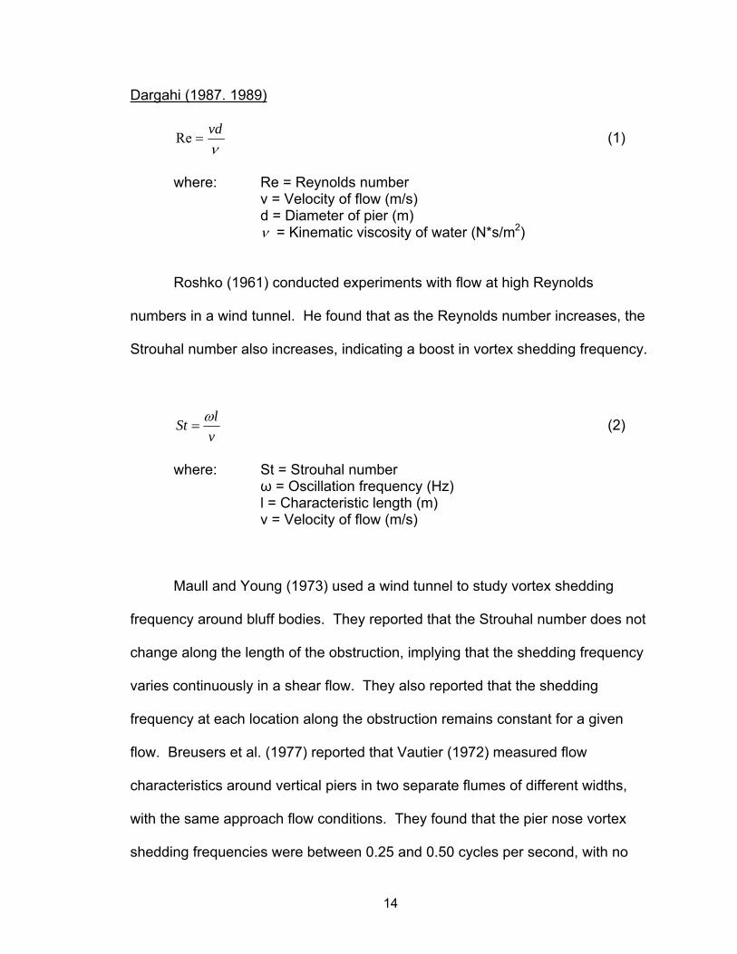
Dargahi (1987. 1989)

νvd

=Re (1)

where: Re = Reynolds number v = Velocity of flow (m/s) d = Diameter of pier (m) ν = Kinematic viscosity of water (N*s/m2)

Roshko (1961) conducted experiments with flow at high Reynolds

numbers in a wind tunnel. He found that as the Reynolds number increases, the

Strouhal number also increases, indicating a boost in vortex shedding frequency.

vlSt ω

= (2)

where: St = Strouhal number ω = Oscillation frequency (Hz) l = Characteristic length (m) v = Velocity of flow (m/s)

Maull and Young (1973) used a wind tunnel to study vortex shedding

frequency around bluff bodies. They reported that the Strouhal number does not

change along the length of the obstruction, implying that the shedding frequency

varies continuously in a shear flow. They also reported that the shedding

frequency at each location along the obstruction remains constant for a given

flow. Breusers et al. (1977) reported that Vautier (1972) measured flow

characteristics around vertical piers in two separate flumes of different widths,

with the same approach flow conditions. They found that the pier nose vortex

shedding frequencies were between 0.25 and 0.50 cycles per second, with no

14

significant difference in either the autocorrelation function or the spectral density

function for flow velocity measurements.

Grecco (1990) observed that a horshoe vortex system undergoes the

following stages as the pier Reynolds number increases: steady single and

multiple vortex regimes, simple oscillation, irregular unsteady motion, transition

and turbulence. The critical Reynolds number from transition to turbulence is

4750. Eckerle and Awad (1991) defined a dimensionless parameter

(ReD)1/3(D/δ), where ReD = Reynolds number, D =depth of flow, and δ =

boundary layer thickness, for a turbulent boundary layer flow. When this

parameter is less than 1000, one horseshoe vortex system exists in the plane of

symmetry; when this parameter is greater than 1000, no vortex is present.

Wen et al. (1993) made comparisons between the vortex systems that

form on a rigid bed at the intersection of the bed and cylinder, and at the

intersection of the cylinder and bed in a scour hole. They found that at the flat

bed (before scour would commence), the vortex system consists of multiple

strong primary (clockwise) vortices as well as weak secondary (counter-

clockwise) vortices. The vortices oscillate upstream then back downstream

before shedding around the pier. The frequency of shedding becomes unstable

as the Reynolds number is increased. The vortex system within a scour hole

generally consists of one vortex which is comparable to the size of the scour

hole. The vortex rotates very slowly, and hence produces a weaker bed shear

stress than in the flat bottom situation. The position of the vortex changes little,

but oscillates slightly for higher Reynolds numbers.

15

Dey et al. (1995) developed a series of equations for velocity profile

predictions in the x, y, and z directions in the upstream, downstream, and in the

scour hole. The circulating and oscillating nature of the flow within the scour hole

made measurements difficult, thereby questioning the applicability of the

equations in this vicinity. Additionally, Dey et al. remarked that because of the

downflow at the front face of the pier impacting the bed, the no-slip condition

cannot be applied, resulting in the disappearance of a boundary layer.

Ahmed and Rajaratnam (1998) analyzed the effects of bottom bed

material on the resulting flow field in the vicinity of cylindrical piers. Three bed

conditions were analyzed: smooth, rough (rigid), and mobile. They found that for

all bed conditions, the effect of the pier on the approaching velocity distribution

can be felt for approximately 2.5 pier diameters in the upstream direction. The

velocity decreases gradually as the cylinder is approached. Near the bed, the

velocity diminished steadily to a point of negativity, which is due to the formation

of the vortex system at the base of the pier. The pressure rises gradually as the

pier is approached. However, the point at which the pressure begins to rise

varies according to the approach flow velocity, suggesting that the presence of

the pier is felt further upstream during flows with higher velocities. Also, larger

piers produced higher pressure values at the face of the pier. Ahmed and

Rajaratnam also found that the downflow produced by the presence of the pier

exhibits a uniform velocity distribution. The maximum downflow velocity was

measured to be as much as 95 percent of the maximum approach flow velocity

once the scour hole was formed. This result was also discovered by Ettema

16

(1980). The maximum downflow velocity before the initiation of a scour hole

reached about 35 percent of the approach flow velocity.

Ali and Karim (2002) reported on the principal features of the flow field

which lead to pier scour. In summary, the flow decelerates as it approaches the

cylinder, coming to rest at the face of the pier. The associated stagnation

pressures are highest near the surface, where the deceleration is greatest, and

decrease downwards. In response to the downwards pressure gradient at the

pier face, the flow reaches a maximum just below the bed level. Ali and Karim

claim that it is this downflow impinging on the bed which is the main scouring

agent. The downflow acts like a vertical jet eroding a trench in front of the pier;

the eroded material then is transported downstream by the development of the

horseshoe vortex. The combination of the downflow and the horseshoe vortex

provides the dominant scour mechanism. They also noted that the scour hole

development commences at the sides of the pier with the two holes rapidly

propagating upstream around the perimeter of the cylinder to meet on the

centerline. Dargahi (1990) noted that the initiation of scour at the sides of the

pier is due to the increased velocities of the flow at the sides of the pier, but that

maximum scour is a result of the downflow and horseshoe vortex which form at

the upstream face of the pier.

Graf and Istiarto (2002) experimentally investigated the flow field in a

scour hole using an Acoustic Doppler Velocity Profiler (ADVP). At the upstream

side of the cylinder, the following results were observed: (1) approaching the

cylinder, the (longitudinal) u-component of velocity diminishes over the entire

17

depth, and begins to show negative values close to the bed; (2) in the approach

region, the (vertical) w-component of velocity remains negligible, but grows

considerably and reaches a value equal to roughly 60 percent of the approach

flow mean velocity; and (3) the (lateral) v-component of velocity remains

negligible but has some small values close to the bed, indicating three-

dimensional flow. In regard to the vorticity of the flow field, they observed: (1) a

positive vorticity is strong at the brink of the scour hole, leading to a weak

counter-clockwise vortex; (2) directly upstream of the cylinder a strong clockwise

vortex is developed; and (3) in the remaining part of the scour hole, the vorticity

is weak and is of the same order as the approach flow vorticity. Shear stress

measurements also were calculated based on the velocity profile and

corresponding Reynolds stresses. The resulting values in the scour hole were

less than the critical values of shear stress presented by Shields (1936), implying

no sediment movement. Turbulence intensities were observed to be very strong

at the foot of the cylinder on the upstream side.

2.4 Numerical Model Simulations

With advancements in computer technology, detailed mathematical

simulation of the flow field in the vicinity of vertical obstructions has become

feasible. Numerical approximations of the Navier-Stokes equations based on

finite difference, finite element, or finite volume solutions have been incorporated

into computer algorithms and used to analyze the mechanics of the scour

problem. Estimations of bottom shear stress, turbulence intensities, and the

18

formation of the vortex systems have been a primary area of focus. The use of

these programs has allowed researchers to analyze the effects of subtle

adjustments to flow variables, which could not be accomplished easily during

laboratory experiments.

Olsen and Melaaen (1993) used a three-dimensional numerical model to

simulate the development of a scour hole. The simulation was based on the

results of a physical model. The scour hole was only partially developed. The

model was completed through 10 iterations of the changing bathymetry of the

scour hole. Although they received encouraging results, Olsen and Melaaen

warned that because the numeric model can not simulate the transient nature of

the oscillating vortices in front of the pier, it may prove faulty for maximum scour

depth predictions.

Mendoza-Cabrales (1993) used the k-ε turbulence closure model to

ascertain the bottom shear stress distribution on a rigid bed in front of a circular

cylinder. His geometric data and flow variables were identical to those used by

Melville and Raudkivi (1977) for a laboratory flume experiment. His results

showed large discrepancies from values measured by Melville and Raudkivi.

Mendoza-Cabrales concluded that the k-ε turbulence closure model is

inadequate for determining the flow field and associated shear stresses in front of

cylindrical objects due to: (1) the inability of the model to handle anisotropic

turbulence of three-dimensional curved flows, (2) the deficiency in representing

the negative contributions to the generation of the kinetic energy of turbulence,

(3) the inability to express the dependency of each component of the Reynolds-

19

stress tensor on one component of the mean strain rate tensor, and (4) the

inability to account for Reynolds-stress relaxation.

In an attempt to produce better results than Mendoza-Cabrales (1993),

Richardson and Panchang (1998) used the Computational Fluid Dynamics model

FLOW-3D to simulate the flow field around a circular pier, based on the

experiments of Melville and Raudkivi (1977). The FLOW-3D model is based on

the solution of the transient three-dimensional Navier Stokes equations by the

volume-of-fluid method. In addition, the model can handle turbulence closure

through a number of accepted schemes, including: Prandtl’s mixing length

theory, eddy viscosity model, two equation k-ε model, and the renormalized

group (RNG) theory. The results of the simulation showed that with proper

calibration of input variables, a flow field similar to the one reported by Melville

and Raudkivi (1977) can be obtained. Shear stress distributions, however, were

said to vary drastically but were not reported. No explanation was given for the

discrepancy. Richardson and Panchang (1998) further showed that by tracking a

single fluid particle at the bottom of a scour hole, predictions could be made as to

a maximum depth of scour by noticing when the particle becomes trapped in the

scour hole. They warned that this may not be a viable method for predicting a

maximum scour depth, unless an accurate representation of geometric data can

be simulated.

Karim and Ali (2000) investigated the suitability of using FLUENT CFD to

model the flow field and corresponding bed shear stress values on a rigid open

channel bed as well as in a non-pier induced scour hole. The geometric model

20

and flow conditions used were based on conditions presented by Ali and Lim

(1986) and Wu and Rajaratnam (1995). The flow field and bottom shear stress

results showed close correlation to the experimental results presented by the

investigators previously mentioned. However, bottom shear stress

measurements were for a location 8 mm above the channel bed. No predictions

of shear on the actual channel surface were made.

Ali and Karim (2002) used the FLUENT CFD computer program to model

the flow structure at a cylindrical pier. Bed shear stresses also were predicted

using the model. Various simulations were performed, representing different

time steps at the development of a scour hole. The geometric and flow

conditions were based on experimental data provided by Yanmaz and Altinbilek

(1991). Analysis of the results showed favorable comparison to the experimental

results of the flow field. However, there was only a fair agreement between the

bed shear stresses predicted by FLUENT and those calculated from the

experimental velocities. This is most likely due to the fact that FLUENT gives on-

bed predictions for shear stress, whereas the ones reported by Yanmaz and

Altinbilek (1991) were at a distance of 8 mm above the bed. While the results

obtained by Ali and Karim are acceptable, they state that using a numerical

model such as FLUENT CFD can not produce truly accurate results due to its

inability to model certain phenomenon such as turbulent bursts or the oscillating

nature of the horseshoe vortex.

21

2.5 Local Scour Predictions

For streams characterized as being on gravel beds, scour depths from

local scour can be much larger than from other scour, i.e., the long-term

degradation and contraction scour. Therefore, for design purposes, maximum

scour depth due to local scour predicted around structures, particularly piers, is

the criteria used for determining the minimum depth at which supporting

foundations are placed. Prediction formulas for local scour depth around piers

are numerous. Some formulas are for clear-water scour, some for live-bed

scour, and some are intended to serve for both. But, due to the complexity of the

problem, most formulas were developed from the limited knowledge of factors

and empirical relations based mostly on laboratory data. A great deal of

discrepancy and even contradictions exist among these formulas. An accurate

prediction using these formulas can be expected only for the cases that are

similar to those utilized to develop the formulas.

The Schoharie Creek Bridge failure in 1987 prompted the development of

a national set of guidelines which is to be used to predict scour depths in the

vicinity of bridges. After the collapse of the bridge, which led to 10 fatalities, the

Federal Highway Administration was commissioned by the federal government to

review any prior studies, either experimental or through field observation, and

based on the results of these studies recommend a series of universal equations

which are to be used to compute the various forms of scour (pier, abutment,

contraction). The result of the study was the creation of HEC-18. This manual

provides national guidelines by which all existing and future federally supported

22

highway bridges are to be evaluated or designed based on scour susceptibility.

The initial pier scour equation utilized in HEC-18 is a variation of the one

developed at the Colorado State University and is based on a set of

dimensionless parameters.

Modified CSU Equation (Richardson et al. 1995) for both clear-water and live-bed

scour:

43.01

65.0

14321

10.2 Fr

yaKKKK

yys

⎥⎦

⎤⎢⎣

⎡= (3)

Where: ys = Scour depth (m) y1 = Flow depth directly upstream of pier (m) K1 = Correction factor for pier nose shape K2 = Correction factor for angle of attack of flow K3 = Correction factor for bed condition K4 = Correction factor for armoring by bed material size a = Pier width (m) Fr1 = Froude number upstream of pier = V1/(gy1)1/2

V1 = Mean velocity of flow upstream of pier (m/s) g = Acceleration of gravity (m/s2)

One parameter not included in Equation (3) is the bed shear stress

generated at the upstream face of a blunt-nosed pier due to the horseshoe

vortex. This omission is noticeable when considering several investigators have

reported in the literature their belief that the horseshoe vortex creates an

estimated increase of shear stress on the bed of 2 to 14 times that of the

upstream approach flow, which in turn drives the scouring process. The

exclusion of shear stress was necessary because in most cases reliable

measurements at the beginning and final stages of the scouring process were

23

not possible due to the limitations of the measuring equipment and its inability to

accurately measure the desired quantities. The goal of this research is to

analyze the time variation of bed shear stress measurements at the base of a

rectangular pier. Based on the results a conclusion will be drawn as the whether

an increase in shear stress is indeed responsible for the initiation of scour around

piers and subsequently if further research is warranted which will lead to the

inclusion of a shear stress parameter in the equations used to predict pier scour.

24

CHAPTER 3

HYPOTHESIS

3.1 Statement of Problem

An increase in shear stress on the channel bottom beneath the horseshoe

vortex has been cited by some researchers to be the primary mechanism for

inducing local scour in non-cohesive soils (Shen 1966a, Breusars et al. 1977,

Baker 1980, Froehlich 1988, Dey et al. 1995, etc.). Much research has been

done in an attempt to quantify an exact value at which the shear is amplified

when compared to the approach flow value, but the results of numerous studies

are not consistent when compared to one another and range from amplifications

in the approach flow shear stress values of 2 to 14 times.

The earliest studies of shear stress magnification were attributed to

Chabert and Engeldinger (1956), who showed that before scour begins, the

shear stress at the pier nose is approximately four times the value in the

approach flow. This is based on the fact that regardless of pier size, scour at the

pier nose begins when U*/U*c >= 0.5, where U* = shear velocity and U*c = critical

shear velocity for particle movement. Schwind (1962) performed an extensive

study of the horseshoe vortex and estimated that the shear stress under it is at

least 12 times the undisturbed value.

Parola (1991) conducted a study of riprap sizes necessary to protect

bridge piers against scour. He concluded that the effective velocity at the base of

a pier must be approximately 1.5 to 1.7 times the approach velocity. Since shear

stress is related to the velocity squared, it follows that Parola’s effective shear

25

stress was 2.2 to 2.9 times the shear stress in the approach. Pagan (1991)

conducted a study similar to Parola’s, and found that the maximum effective

shear stress at the base of abutments represented an amplification of

approximately four times the average shear stress in the approach flow.

Johnson and Jones (1992) used marbles in a scour hole to indirectly

measure the shear stress at the base of a pier at various scour depths. They

concluded that the effective shear stress at the base of a pier varied from 2.8 to

14 times the shear stress in the approach flow, depending on the depth of scour.

Ahmed and Rajaratnam (1998) approximated shear stress measurements

on the channel bottom at the pier using two three-tubed yaw probes. They

measured an average increase of bed shear stress of 10-12 times, with a

maximum of 13.5, the amount in the approach flow for rigid and mobile beds.

However, for the smooth bed experiments, the amplification was much less (6

times) and also was confined to a smaller area around the pier. They also found

that once the scour hole begins its formation, the distribution of shear stress

decreased substantially at the sides of the pier, while increasing upstream of the

pier.

Annandale (1999) proposed an erodibility index method for estimating

scour limits in rock formations based on average stream power. He found that

the approach stream power is amplified by 7.6 to 12.6 based on pier shape.

Assuming that the shear stress is proportional to the stream power raised to the

2/3 power, it follows that the corresponding shear stress amplifications range

from 3.9 to 5.4.

26

Jones (2002) performed experiments using sand particles and Shield’s

criteria for critical shear stress to estimate the amount of shear stress

amplification at the base of a pier. He plotted a dimensionless shear stress

parameter vs. a dimensionless depth parameter in order to develop a relationship

of how shear stress varies according to scour depth. By extrapolating his data to

a point of zero scour, he found that shear stress generally is amplified at the

base of a pier by six times the amount in the approach flow. He then performed

experiments on a rigid boundary using Particle Image Velocimetry (PIV) to

ascertain the shear stress amounts. PIV has the ability to solve for shear stress

directly using the definition of total shear stress based on Newton’s law of

viscosity and the Reynolds turbulent stresses. Using PIV, Jones found that the

shear stress in front of a pier is amplified by 6.2. However, he cautioned that the

results of the PIV analysis were very subjective as amplification values could

have ranged from less than one up to 95.

Other researchers disagree in the assumption that an increase in shear

stress induces pier scour and believe that the driving mechanism of scour is the

downflow reflecting off the pier which subsequently impacts the channel bottom

and erodes the soil; the horseshoe vortex system is only responsible for

transporting the sediment once it is no longer attached to the bed (Melville 1975,

Ettema 1980, Rajaratnam 1980, Raudkivi and Ettema 1983, etc.). The reason

for such differences of opinion is that no actual physical measurements have

ever been made of the shearing forces at the base of a blunt-nosed pier. In each

27

of the studies noted previously, assumptions were made about shear stress

values through the measurement of more quantifiable variables.

This research, through the use of a force-displacement sensor which was

calibrated to yield shear stress values, investigated the temporal variation of

shear stress values generated at the base of rectangular piers. The results are

used to ascertain a better understanding of the mechanisms which lead to local

scour around vertical obstructions.

3.2 Hypothesis

Several investigators (Chabert and Engeldinger 1956, Shen 1966a,

Melville 1975, Raudkivi and Ettema 1983, etc.) have shown pier scour will not

commence until the approach shear velocity has reached half the critical shear

velocity for incipient motion. Because shear is directly proportional to the shear

velocity squared, it follows that the shear in front of a pier theoretically should be

approximately four times the approach flow shear.

ρτ 2*uo = (4)

Where: τ o = Average boundary shear stress (Pa) u* = Shear velocity (m/s) ρ = Density of water = 1000 (kg/m3)

The underlying hypothesis for this research project is: scour is initiated by

an increase of bed shear stress at the base of a pier of at least four times the

approach flow shear stress.

28

oimumpier ττ 4)(max ≥ (5)

where: )(max imumpierτ = Maximum peak shear (Pa) oτ4 = Four times the average approach shear (Pa)

3.3 Hypothesis Verification

“Level Crossing Statistics” (explained in Chapter 8) are used to verify the

proposed hypothesis. In particular, the magnitude and duration of the shear

values above the approach flow shear stress are analyzed. Additionally, the

periodicity and frequency of the measurements are found and used to determine

if the vortex is “felt” on the channel bottom and responsible for the measured

shear peaks.

29

CHAPTER 4

EXPERIMENTAL SETUP

4.1 Experimental Equipment

All experiments were conducted in a rectangular recirculating flume

approximately 2.75 m long, .46 m wide and .30 m deep. A shear stress

measuring device (Figure 4.1), designed by Mr. Hans Prechtl (2002), was used

to measure all shear stress values. The device has the advantage of measuring

actual forces which are captured through an electrical carrier signal. The

electrical signal was calibrated to yield an applied shear stress. The

specifications of the shear stress measuring device follow:

Figure 4.1 - Shear stress measuring device

30

Principles of Operation - The sensor consists of a stable aluminum case with a shaft (~ 300 mm) in it, which is ball-beared about 100 mm from the top. On the top of the shaft a carrier is mounted, on which the segments under test are attached. The force of the flowing water excites the segment under test to max +/- 1 mm displacement from its quiescent state. About 100 mm under the pivot two bronze-springs are fixed. The deviation of the shaft is transferred to the springs by a highly flexible tension-band. So, each deviation of the shaft bends the resistance strain gauge, which gives in consequence an electrical signal to the connected carrier bridge. The force, which is necessary to bend the bronze-springs +/- 1 mm, is called Narrow Span. In the existing sensor the Narrow Span is about +/-0.06 N. To increase the measurement-range, a tension spring is mounted at the lower end of the shaft: pulling this spring will increase the force for the same amount of deviation (+/- 1 mm). A log-scale on the micrometer screw enables the user to set a predefined measurement-range for the sensor. In the existing design the final range was set to ~ 1N. Moreover the final range depends mainly on the spring-factor, whereby it may be adapted to the experimental arrangement by exchanging this spring. The installation on the channel-floor is done very simply by some mounting-holes for the flange and one center-hole of 15 mm diameter, for the carrier. To compensate for various thicknesses of the channel wall, the carrier is moveable on the shaft to about +/- 10 mm. At the carrier, the segments under test can be easily exchanged by loosening 3 small screws. The sensor has to be mounted vertically on the channel floor. To compensate for aberrations from this state, adjustment facilities are also provided on the sensor. The constructive design makes the sensor in a wide range insensitive against temperature changes, assembling works at the segment and the carrier, water-level and water impurities. (Prechtl 2002)

The panel exposed to the fluid used to measure the applied force is

rectangular in shape, approximately 5 cm per side. The device itself yields only

an average shear stress over this area. Calibration of the device was achieved

both statically and dynamically (see Chapter 5 for a detailed description of the

31

calibration process and identification of fluid forces). At its lowest setting, in a

static case, the device can measure shear stresses ranging from 0 to 2 Pa

(results from this study ranged from -0.3 to 0.5 Pa). Due to the sensitive nature

of the measuring device (i.e. – fluctuations due to surrounding air disruptions) a

new support structure was designed and built for the flume to make it sturdier

and less prone to vibrations (Figure 4.2). The support structure consists of rigid

I-beam steel construction with four legs .45 m high welded to floor plates; two .51

m beams at either end of the structure are used to connect the legs in the lateral

direction, and two 2.64 m beams are used to connect the legs in the lengthwise

direction.

Figure 4.2 - Flume support structure

32

A water tank approximately 1 m cubed was fabricated out of 1.9 cm thick

clear plexi-glass and was used to store water supplied to the flume. A Chemflo

Type 3 378 LPM pump with an impeller diameter of .133 m made of stainless

steel construction was used to drive the water from the tank to the flume. The

pump has a suction diameter of 5 cm and a discharge diameter of 3.8 cm. A

Saftronics Rapidpac GP-10, variable torque, variable speed control unit, pulse

with modulating variable frequency drive was used to control the speed of the

pump and hence the overall discharge. A dolly made of steel construction

approximately 1 m wide by 1.5 m long was used as a platform to secure the tank

and pump, making it external from the flume. This was necessary to reduce

inherent vibrations caused by the pumping system (Figure 4.3).

Figure 4.3 - Tank/pump/motor controller/support dolly

33

A Kobold Turbine Flow Sensor with 0-10 VDC output signal and a range of

20-333 LPM (+/- 1%) was used to measure the flow entering the flume. The

depth of water in the flume was controlled using a 10 cm CPEX true union ball

valve placed externally at the exit of the flume. Water depth was measured to

within an accuracy of 0.3 mm using a Baumer Electric Depth meter. The velocity

distribution of the approach flow was measured using a Marsh-McBirney Electro-

Magnetic Water Current Meter. A mobile carriage system built of ITEM

CONSTRUCTION pieces was assembled and used to house the flow depth

meter and velocity probe. The carriage system allowed for three degrees of

freedom of the velocity probe (Figure 4.4).

Figure 4.4 - Carriage system used to house velocity probe

The piping system consisted of 5 cm PVC pipe going from the water tank

to the pump, and 3.75 cm PVC pipe from the pump to the flow meter and then

into the flume. A 10 cm PVC pipe carried the water from the exit of the flume,

through the control valve and back into the water tank.

34

Figure 4.5 - Experimental setup showing tank/pump/motor controller/flume/carriage system

35

CHAPTER 5

IDENTIFICATION OF FLUID FORCES

5.1 Initial Offset Adjustment

The shear measuring device has an aluminum rod which extends out of

the sensor casing and is topped with a flat plate which is exposed to water

flowing over the sensor and through the flume (Figure 5.1). A very thin rubber

membrane surrounds the aluminum rod and is used as a border separating the

inner casing of the sensor and the outer environment (Figure 5.2). The

membrane is flexible in allowing the rod to move when exposed to a tangential

force applied over the flat plate, but secure enough to not allow any water to leak

into the sensor casing which contains the strain gages and electrical

components.

Figure 5.1 - Aluminum rod protruding from top (right) of sensor

36

Rubber Membrane

ed at base of well in sensor

Because the membrane is flexible in allowing the rod to move, but also

ng

r

us

the

Figure 5.2 - Rubber membrane locat

secure in that it stays fastened to the rod and surrounding casing, any force

applied to the membrane also will cause displacements to the rod. When in a

normal state, not exposed to any water, the sensor can be balanced to yield a

zero voltage produced from the strain gages. However, when ponding water is

applied to the sensor and its inner well, the membrane flexes due to the applied

normal force of the water and hence causes deviations in the vertical rod

alignment. Therefore, calibration was performed in order to develop a rati

curve of an applied downward force due to the weight of the water vs. plate (o

rod) displacement. This calibration was achieved by ponding water at various

depths and recording subsequent voltage readings produced from the inner

strain gages. The calibration was performed at the beginning, end, and vario

midpoint intervals during each day of experimentation. Each trial produced

nearly identical calibration equations, which ultimately were used to filter out

effects of sensor displacement due to the weight of the water acting normally

37

over the sensor plate. A total of 15 trials were completed. Tables 5.1 lists the

results of one such calibration. Figure 5.3 shows the corresponding trend line

with best fit equation and R

Table 5.1 – Depth of flow vs. voltage - calibration data

(cm) voltage

2 value used for the adjustment.

depth

8.4 -1.25 8.03 -1.23 7.54 -1.17 7.15 -1.11 6.75 -1.06 6.38 -0.99

6 -0.93 5.63 -0.87

5.24 -0.81 4.82 -0.74 4.48 -0.69 4.04 -0.62 3.68 -0.56 3.31 -0.49 2.95 -0.44 2.6 -0.38 2.26 -0.32

2 -0.28 1.72 -0.24

0 0.05

38

y = -0.1609x + 0.0383R2 = 0.9995

-1.4-1.2

-1-0.8-0.6-0.4-0.2

0

0 2 4 6 8

Depth (cm)

Volta

ge (v

)

10

Figure 5.3 – Calibration curve with corresponding best fit equation used to adjust voltage signal offset caused by weight

of water displacing sensor rod

5.2 Dynamic Calibration

The shear sensor used as part of this research can be considered a

Flow Induced Structure with corresponding stiffness and damping (Figure 5.4).

For a flow induced system operating at a low frequency (ω<<ωn) such that it may

be considered quasi-static, the structural response of the system can be

approximated to be proportional to the instantaneous exciting force exerted by

the flow. However, if the force driving the system is operating at or near a

frequency equal to that of the resonance of the system, the system may respond

non-linearly (Figure 5.5). Because the voltage signal reported as output from the

sensor, and used to determine an applied shear stress over the sensor, is

directly related to the displacement of the sensor and not the driving force of the

39

flow, a dynamic calibration of the sensor is necessary in order to determine the

actual shear generated by the flow.

Fmean + F’ xmean + x’

where: F = Force (N) x = Displacement (m)

Stiffness

Damping

m

k k

C

Figure 5.4 - Graphical representation of shear sensor plate with pivoting rod and associated stiffness and damping

40

1.0

D

ωnω

Quasi-static range

Dynamic range

Figure 5.5 – Variation of dynamic magnification factor with frequency

A dynamic calibration can be completed once the stiffness, damping, and

natural frequency of the sensor are known. The above properties are used to

determine the unit impulse response function which then is used in combination

with the response signal of the sensor to determine the input signal supplied by

the flow as follows (Naudascher and Rockwell 1994):

( ) ( ) ( iii GHS )ωωω ⋅= (6)

where: S(ωi) = Response signal of sensor in the frequency domain (Hz)

H(ωi) = Unit impulse response function of sensor in the frequency domain (Hz)

G(ωi) = Input signal supplied by flow in frequency domain (Hz)

41

Equation (6) can be rearranged to yield the input signal and hence driving

force of the flow as follows:

( ) ( )( )i

ii H

SG

ωω

ω = (7)

The unit impulse response function of the sensor in the time domain is

determined from Equation (8):

( ) ( ttm

th ξωωω

expsin1)( = ) (8)

where: h(t) = Unit impulse response function (V) m = Mass of system (kg) ω = Natural frequency of sensor (Hz) t = Time (s) ξ = Damping (%)

The procedure used to determine the driving force of the flow is:

a) The unit impulse response function of the sensor is calculated

based on the dynamic properties of the sensor (Equation 8).

b) The unit impulse response function is converted from the time

domain to the frequency domain using a FFT.

c) The response signal from the sensor is obtained through

experimental measurements.

d) The response signal of the sensor is converted to the frequency

domain using a FFT.

42

e) The response signal in the frequency domain is divided by the unit

impulse response function in the frequency domain (Equation 7).

f) An inverse FFT is performed on the resulting signal from step (e) to

give the driving force of the flow in the time domain.

The flow chart in Figure 5.6 describes the overall process used to

determine the driving force of the flow.

g(t) Fluid force in time

domain

h(t) Unit impulse

response function of sensor in time domain (eq 7 –

known)

s(t) Response signal in

time domain (measured)

FFT

FFT

H(iω) Unit impulse

response function in frequency

domain

S(iω) Unit impulse

response function in frequency

domain

( )( ) ( )ωωω iGiHiS

=

Fluid force in

frequency domain

Governing convolution equation – g(t)*h(t)=s(t) Need to determine g(t)

Inverse FFT

Figure 5.6 – Flow chart depicting procedure used for determining force delivered by flow to sensor

43

5.2.1 – Determination of Dynamic Properties

5.2.1.1 - Stiffness/Damping

The stiffness of the sensor can be obtained through a static calibration

measurement of Force vs. Displacement. When exposed to tangential forces,

the shear measuring device yields a voltage signal produced by a series of four

strain gages and electrical resistors and wires used to transmit the signal. The

voltage signal is captured by a Phillips Bridge Supply Frequency Converter

(Figure 5.7).

Figure 5.7 - Phillips frequency converter used to capture voltage signal delivered by shear sensor

A calibration curve was created by exposing the sensor to a series of

increasing vertical forces and recording the electrical response of the strain

gages in terms of voltage. A moment analysis of the system (Figure 5.8) then

was used to convert the vertical forces to an applied horizontal force. A

44

relationship then was developed between the applied horizontal force divided by

the plate area, and the electrical response of the strain gages in terms of voltage.

F1 F2

L1

L2 L1*F1 = L *F

Figure 5.8 – Static calibration technique using known vertical forces and moment arm lengths to determine tangential forces

A total of six curves were produced, three representing an applied force in

the positive direction and three in the negative direction. Each curve produced

nearly identical results. Table 5.2 lists the results of one such calibration. Figure

5.9 shows the corresponding trend line with best fit linear equation and R2 value.

The best fit linear equation will be used later as part of the error analysis of the

system (Section 6.3). The stiffness of the device is then equal to the slope of the

calibration curve, after adjusting for Force vs. Displacement in lieu of Shear vs.

Voltage. The stiffness in air was found to equal 4.5 N/m.

45

Table 5.2 –Shear vs. voltage - In-air stiffness determination data

Shear (Pa)

Voltage (V)

.03 .010

.07 .035

.12 .059

.24 .120

.36 .189

.48 .290

.60 .351

.72 .419

.85 .480

.97 .545 1.09 .607 1.21 .679 1.33 .742 1.45 .807 1.57 .877 1.70 .936 1.82 1.00 1.93 1.06

y = 1.8013x + 0.0003R2 = 0.9991

0

0.5

1

1.5

2

2.5

0 0.2 0.4 0.6 0.8 1 1.2

Voltage (V)

She

ar (P

a) B

ased

on

Plat

e Ar

ea o

f 5cm

x 5

cm

Figure 5.9 – Determination of stiffness of sensor by exposure to tangential shearing forces in air

46

It next was necessary to determine if the stiffness of the device changed

under aquatic conditions. In order to determine the stiffness, weights of known

densities and volumes were created and used to measure the forces in a similar

manner as when in air. A total of three weights were manufactured, composed of

steel with a specific weight of 76,700 N/m3. The weights had a peg-like shape

and their volumes varied from 9.8 x 10-9 m3 to 2.4 x 10-7 m3.

Two holes were drilled on the ends of the shear measuring plate and used

to position the calibration weights (Figure 5.10). The location of the holes was

recorded to within .5 mm of their length to the center of the shear plate. Both the

measured distances of the drilled holes and the known volume and weight of the

pegs were used in a moment analysis similar to that explained previously. A total

of 12 measurements were taken, varying the depth of water for each set of trials

in order to ascertain if the depth of water added any additional resistance while

calibrating. Each trial produced nearly identical results, indicating that the depth

of water did not affect the amount of resistance encountered. Table 5.3 lists the

results of one such calibration. Figure 5.11 shows the corresponding trend line

with best fit linear equation and R2 value. Adjusting the curve for Force vs.

Displacement shows the stiffness under water equal to approximately 5.5 N/m.

This stiffness is slightly higher than the one found in air; however, the range of

forces used to compute the stiffness was not complete and only accounted for

small displacements of the sensor. Because the sensor is expected to operate

under the full range of displacement, a stiffness of 4.5 N/m was used as part of

47

the sensor calibration process. The possible affect of using this stiffness in place

of the measured stiffness under water is discussed in Section 6.3.

Typical Shape of Calibration Weight

Plan View of Measuring Plate with Calibration Hole Locations

2.2 cm

Figure 5.10 – Schematic of calibration weight/measuring plate

used for stiffness determination under aquatic conditions

Table 5.3 –Shear vs. coltage - aquatic stiffness determination data

Shear (Pa)

Voltage (V)

0.00 0.00 0.258 0.12 .483 0.22

48

y = 2.1842xR2 = 0.9998

0

0.1

0.2

0.3

0.4

0.5

0.6

0 0.05 0.1 0.15 0.2 0.25

Voltage (V)

Shea

r (P

a) B

ased

on

Pla

te A

rea

of 5

cm x

5 c

m

Figure 5.11 – Determination of stiffness of sensor when exposed to tangential shearing forces in water

The damping of the sensor is a measure of how the sensor will decay after

a sudden excitation. This value was determined by the manufacturer and

reported to equal 8 percent.

5.2.1.2 – Natural Frequency/Mass

If a flow induced structure is excited by a turbulent signal, it will respond

around its natural frequency in spite of the fact that the natural frequency may not

coincide with the dominant frequency of the excitation. This can be shown when

plotting the amplitude spectrum of the response signal (Naudasher and Rockwell

1994) (Figure 5.12).

49

Background response

Resonance response

Am

plitu

de S

pect

rum

ωn ω

Figure 5.12 – Typical response of flow induced structure in frequency domain depicting peak amplitude at natural frequency of the structure

The shear sensor was allowed to respond freely under dynamic conditions

induced by free surface flow moving across the sensor, at various depths. The

response of the sensor was ascertained and then converted to the frequency

domain using a Fast Fourier Transform of the data as shown in Figure 5.13.

Based on the results of the various tests, the sensor is found to have a natural

frequency equal to 9.0 Hz.

50

0

0.0001

0.0002

0.0003

0.0004

0.0005

0.0006

0.0007

0.0008

0 5 10 15 20 25

Frequency (Hz)

Am

plitu

de S

pect

rum depth = .151 ft

depth = .169 ftdepth = .183 ftdepth = .195 ftdepth = .207 ftdepth = .220 ft

Figure 5.13 – Amplitude spectrum of response measurements of sensor at various flow depths, showing a natural frequency of 9.0 Hz

With a natural frequency of 9.0 Hz and a stiffness of 4.5 Hz, the mass of

the system responding in the direction of flow can be determined by Equation (9):

mK

=2ω (9)

where: ω2 = Natural frequency of sensor = 9.0 Hz K = Stiffness of sensor = 4.5 N/m m = Mass of sensor (kg)

Rearranging and solving Equation (9) shows a mass of .0014kg. With known

mass, stiffness, damping, and natural frequency, Equation (7) is used in

combination with the response signal of the sensor, according to the procedure

outlined in Figure 5.6, to determine the fluid forces causing the sensor to

displace.

51

CHAPTER 6

DATA COLLECTION

6.1 Autocorrelation Function/Correlation Length

A sufficient number of samples need to be collected in order to ensure

statistical independence from adjacent measurements. The number of samples

and frequency of measurements are determined by analyzing the autocorrelation

function of a long time series of measurements at a very high sampling rate

(Ermshaus 1985). Once the measurement is taken, the variance of the data is

determined and used in conjunction with a predetermined statistical tolerance in

order to determine the number of samples, also known as the correlation length.

The precision chosen for the measurements was 0.005 Pa at 2 standard

deviations, or a 96 percent confidence interval. The number of samples then is

determined by use of the following equation:

2

2

x

xNσ

σ= (10)

where: N = Number of samples for statistical independence from adjacent measurements

2xσ = Variance of measurement

2xσ = Precision of measurement at 2 standard deviations

= 00000625.2

005. 2=⎟

⎠⎞

⎜⎝⎛

A long time series of shear measurements was taken at the base of a pier

with a shallow depth and high Froude number in order to determine the

maximum number of samples needed for the remaining experiments. The

52

combination of shallow and fast moving water produced the greatest variance of

0.06. Using this value of 0.06 in Equation (10) yields an upper limit of 10,400

samples to ensure statistical independence from adjacent measurements. A

safety factor of over 10 percent was added, resulting in a total of 12,000 samples

taken for each trial.

The frequency of the data measurements also is determined via the

autocorrelation function (Ermshaus 1985). The autocorrelation function for the

trial with the highest variance is shown in Figure 6.1.

Autocorrelation Function

-0.06

-0.03

0

0.03

0.06

-12000 -6000 0 6000 12000

Time

Auto

corr

elat

ion

Figure 6.1 - Autocorrelation function of test run with highest variance used to determine minimum sampling frequency

53

In order to determine the minimum frequency for data collection, the

correlation coefficient was found and then integrated. The correlation coefficient

is equal to the autocorrelation function divided by the variance of the data string.

The frequency then is determined by calculating the reciprocal of the area

obtained through integration. A minimum frequency of 40 Hz was determined

using this procedure. Since a large aspect of this research is analyzing the peak

shear values of the measurements, the frequency of data collection was

increased 200 Hz for all trials. This increase insured that all peaks were

captured during data measurements.

6.2 Data Collection Procedure

Several trials were completed with Froude numbers varying between 0.1 -

0.56 for unobstructed flow and 0.13 – 0.45 for obstructed flow. The flow

conditions were set by increasing or decreasing the speed on the variable

frequency drive, used to control the speed of the pump. A minimum speed on

the drive associated with 40 Hz was set as the lower limit. This speed led to flow

depths of .065 ft and Froude numbers of 0.56. A minimum of three trials was run

at this drive setting and the results were recorded. The drive then was increased

in speed in increments of 5 Hz, and data collected. A total of 69 trials for

unobstructed flow and 60 trials with a pier were completed.

54

6.3 Data Collection Errors

The possibility of obtaining an error in the data collected during any

laboratory experiment is high. Two types of error typically are encountered:

human error and equipment error. The possible human errors present in this

work stem primarily from the initial calibration of the data collection equipment,

i.e., depth sensor, flow sensor, shear sensor, etc. During the calibration of each

of the measuring devices, human judgment was necessary. Specifically, human

errors could have resulted during the following tasks:

• Calibration of the flow depth sensor – depths of flow needed to be

measured using a length scale (ruler) and then cross-correlated with

voltages read by the sensor. Calibration curves then were created relating

the human-read depths and applied voltages. The human read

measurements are estimated to be within 2 mm. Errors associated with

the flow depth sensor have a direct influence on Froude number

computations used for data analysis. The reported Froude numbers are

calculated based on collected data and are accurate to within 0.02.

• Initiation of shear sensor – before any measurements were taken with the

shear sensor, the sensor needed to be zeroed according to the analog

voltage display frequency converter (Figure 5.9). The only way to zero

this device is through a voltage adjustment knob on the face of the

frequency converter. The knob was turned until the needle displaying the

voltage was in a nearly completely vertical position, indicating a zero

reading. A digital display device was used to verify the analog reading of

55

the frequency converter at several points during the calibration process.

The digital display showed actual voltages ranging from 0 to +/- 0.02 Volts.

When using an initial offset of +/- 0.02 Volts in the static calibration

equation developed under aquatic conditions (Figure 5.13) an error in

shear of 0.04 Pa is produced.

• Improper sensor stiffness coefficient – The effect of changing the stiffness

coefficient from 4.5 N/m to 5.5 N/m was determined by changing the value

input as part of the calibration procedure and re-calculating the results.

The outcome indicates a change in shear output ranging from .005 Pa at

lower Froude numbers to .010 Pa at higher Froude numbers.

6.3.1 Equipment Error

All of the data collection equipment used for this study was based on the

principle of an electrical voltage signal being given by the device which would

then correspond to some physical quantity (depth, flow, shear, etc.). For some of

the equipment (flow meter, depth meter, shear sensor), a minimum voltage

needed to be obtained before the output of the device could be considered

accurate. The flows and depths used throughout this study were above the

minimum voltage requirement (as suggested by the manufacturer); therefore, the

errors produced by these devices should lie within the error bounds supplied by

the equipment manufacturer – 0.3 mm for the depth meter, one percent of total

flow for the flow meter. For the shear sensor, however, no such minimum

voltage requirement was supplied by the manufacturer; therefore, the amount of

56

error generated by the sensor had to be calculated based on calibration curves

relating the voltage signal to an applied shear stress. As mentioned in Section

5.2.1.1, a total of six curves were created relating the voltage signal to an applied

shear stress. Each curve was derived using the same calibration weights;

therefore, in an ideal situation all six curves would be identical. The results of

each calibration showed slight discrepancies in the final calibration equation.

However, these discrepancies were small and in the range of only +/- 0.005 Pa

for any particular voltage reading.

Combining human and equipment error, the sensor is considered to be

accurate to within +/- 0.05 Pa.

57

CHAPTER 7

UNOBSTRUCTED FLOW

7.1 Results

A total of 69 experiments were completed using the shear measuring

device. The purpose of the experiments was to ascertain a relationship between

the uniform flow Froude number and an applied shear stress over the measuring

plate. The relationship will be later used to ascertain an “approach flow shear

stress” and how this value compares to a time series of shear measurements in

front of a vertical obstruction. The results are listed in Table 7.1 and displayed

graphically with corresponding error bars in Figure 7.1.

Table 7.1 – Unobstructed flow results

Trial Name

Q (lps)

Depth (cm)

Velocity (cm/s)

Froude # Shear avg Shear St. Dev.

40_1H 2.0 5.2 0.3 0.12 0.23 0.02 40_2H 2.0 5.2 0.3 0.12 0.22 0.02 40_3H 2.0 5.2 0.3 0.12 0.22 0.02 40_1L 2.2 2.0 0.8 0.56 0.57 0.07 40_2L 2.2 2.0 0.8 0.55 0.51 0.06 40_3L 2.2 2.0 0.8 0.56 0.53 0.06 45_1L 2.6 2.2 0.8 0.55 0.52 0.05 45_2L 2.6 2.2 0.8 0.55 0.53 0.04 45_3L 2.6 2.2 0.9 0.55 0.53 0.04 50_1H 2.8 5.6 0.4 0.14 0.24 0.02 50_2H 2.8 5.6 0.4 0.14 0.24 0.02 50_3H 2.8 5.6 0.4 0.14 0.24 0.02 50_2L 2.9 2.4 0.9 0.53 0.47 0.05 50_4L 2.9 2.5 0.9 0.52 0.38 0.11 50_5L 2.9 2.5 0.8 0.51 0.46 0.09 50_6L 2.9 2.5 0.9 0.53 0.38 0.11 55_1L 3.3 2.8 0.8 0.47 0.35 0.05 55_2L 3.3 2.8 0.8 0.48 0.32 0.05 55_3L 3.2 2.9 0.8 0.46 0.32 0.05 55_6L 3.2 2.8 0.8 0.48 0.38 0.08 60_1H 3.5 6.0 0.4 0.16 0.26 0.03 60_2H 3.5 5.9 0.4 0.16 0.26 0.02 60_4H 3.5 5.9 0.4 0.16 0.26 0.02

58

Trial Name

Q (lps)

Depth (cm)

Velocity (cm/s)

Froude # Shear avg Shear St. Dev.

60_5H 3.5 6.0 12.9 0.17 0.26 0.03 60_1L 3.6 3.1 25.0 0.45 0.33 0.04 60_2L 3.6 3.1 24.8 0.45 0.33 0.05 60_3L 3.6 3.2 24.3 0.43 0.33 0.04 60_4L 3.5 3.2 24.2 0.43 0.32 0.04 65_1L 3.9 3.4 25.1 0.44 0.39 0.08 65_2L 3.9 3.4 24.7 0.43 0.37 0.08 65_3L 3.9 3.4 24.7 0.43 0.37 0.08 67_1L 4.0 4.0 21.9 0.35 0.35 0.02 67_2L 4.0 3.8 23.0 0.38 0.36 0.02 67_3L 4.0 3.8 22.9 0.37 0.36 0.02 70_1H 4.1 6.3 14.2 0.18 0.28 0.02 70_2H 4.1 6.3 14.3 0.18 0.28 0.02 70_3H 4.1 6.3 14.1 0.18 0.28 0.02 70_4H 4.1 6.3 14.1 0.18 0.28 0.04 70_1L 4.2 3.2 28.6 0.51 0.36 0.08 70_2L 4.2 3.2 28.7 0.51 0.38 0.10 70_3L 4.1 3.4 26.6 0.46 0.39 0.08 75_4L 4.4 3.4 28.7 0.50 0.36 0.07 75_5L 4.4 3.4 28.7 0.50 0.37 0.07 75_6L 4.4 3.4 28.9 0.50 0.34 0.07 75_7L 4.4 3.4 29.0 0.51 0.35 0.07 80_1H 4.7 6.6 15.7 0.19 0.28 0.02 80_2H 4.7 6.6 15.7 0.19 0.28 0.03 80_8H 4.7 6.6 15.6 0.19 0.28 0.02 80_9H 4.7 6.6 15.5 0.19 0.29 0.03

80_10H 4.7 6.8 15.2 0.19 0.27 0.03 80_11H 4.7 6.6 15.5 0.19 0.27 0.02 80_1L 4.7 3.9 26.7 0.43 0.35 0.04 80_2L 4.7 3.9 26.7 0.43 0.36 0.04 80_3L 4.7 3.9 26.7 0.43 0.35 0.04 85_1L 5.0 5.0 21.8 0.31 0.32 0.03 85_2L 5.0 5.8 19.0 0.25 0.31 0.03 85_3L 5.0 5.0 22.1 0.32 0.32 0.04 90_1H 5.3 7.3 15.9 0.19 0.29 0.03 90_2H 5.3 7.3 15.8 0.19 0.29 0.02 90_3H 5.3 7.3 15.8 0.19 0.29 0.03 90_1L 5.3 5.9 19.7 0.26 0.32 0.04 90_2L 5.3 5.9 19.6 0.26 0.30 0.04 90_3L 5.3 6.0 19.2 0.25 0.31 0.04 94_1H 5.5 7.5 16.0 0.19 0.30 0.03 94_2H 5.5 7.6 15.9 0.18 0.29 0.03 94_3H 5.5 7.5 16.0 0.19 0.29 0.03 94_1L 5.5 6.8 17.8 0.22 0.31 0.04 94_2L 5.5 6.5 18.6 0.23 0.31 0.04 94_3L 5.5 6.3 19.1 0.24 0.33 0.04

59

0.0

0.1

0.2

0.3

0.4

0.5

0.6

0.7

0.0 0.1 0.2 0.3 0.4 0.5 0.6Froude Number

Shea

r (Pa

)

Figure 7.1 – Graphical display of results of shear vs. Froude number with corresponding error bars (+/- .05 Pa) obtained from the unobstructed flow analysis

7.2 Analysis

For Froude numbers ranging from 0.1 - 0.4, there is an increase of shear

with Froude number. This increase is expected when considering that the bed

shear on a channel bottom is directly proportional to the shear velocity squared

(Equation 4), and the shear velocity is proportional to the coordinate velocity of

the flow (Equation 11) (assuming a logarithmic velocity distribution of the flow).

Additionally, the Froude number is also directly proportional to the mean velocity

of the flow (Equation 12); therefore, an increase in mean velocity which leads to

an increase in Froude number should translate into an increase in bed shear.

60

ByuLnku

u+⎟

⎠⎞

⎜⎝⎛=ν*

*

1 (11)

where: u = Coordinate velocity (m/s) u* = Shear velocity (m/s) k = Prandtl’s constant = 0.4 y = Depth (m) ν = Kinematic viscoity (m2/s) B = Constant of integration

gyuFr channelrect =_ (12)

where: Fr = Froude number in a rectangular channel u = Mean velocity of flow (m/s) g = Constant of gravity = 9.8 m/s2

y = Depth of flow (m)

For Froude numbers ranging from 0.40-0.52 the increasing trend ceases,

a lot of scatter is present, and shear appears to be independent of Froude

number. The hydraulic conditions of the flow were checked at these Froude

numbers and it was noticed that the depths of flow ranged from approximately

1.0 to 1.5 inches. Additionally, it was observed during the experiments that for

the trials executed at shallow water depths (< 1.5 inches), noticeable surface

waves were present; whereas for higher water depths, a nearly uniform flow was

achieved (according to visual observation). The existence of these surface

waves produces a non-uniform flow resulting in greater fluctuations in the shear

values reported by the sensor. These fluctuations should be identifiable in the

standard deviation of shear measurements from each trial (Figure 7.2).

61

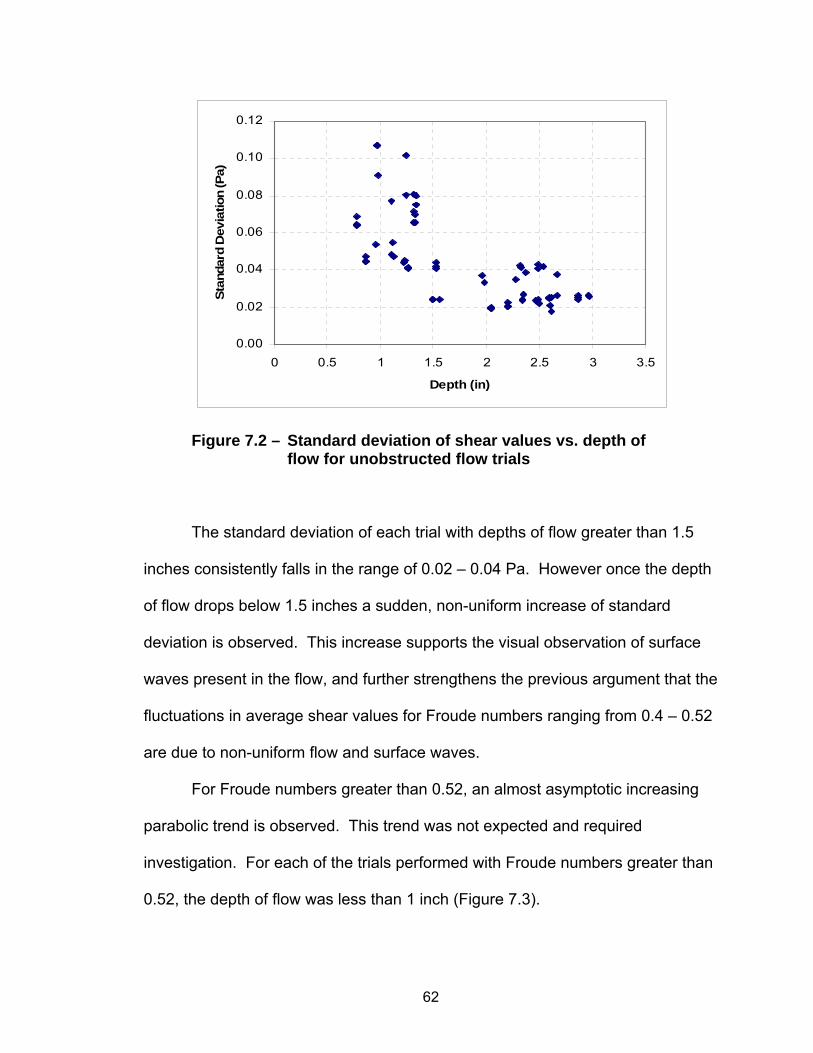
0.00

0.02

0.04

0.06

0.08

0.10

0.12

0 0.5 1 1.5 2 2.5 3 3.5

Depth (in)

Stan

dard

Dev

iatio

n (P

a)

Figure 7.2 – Standard deviation of shear values vs. depth of flow for unobstructed flow trials

The standard deviation of each trial with depths of flow greater than 1.5

inches consistently falls in the range of 0.02 – 0.04 Pa. However once the depth

of flow drops below 1.5 inches a sudden, non-uniform increase of standard

deviation is observed. This increase supports the visual observation of surface

waves present in the flow, and further strengthens the previous argument that the

fluctuations in average shear values for Froude numbers ranging from 0.4 – 0.52

are due to non-uniform flow and surface waves.

For Froude numbers greater than 0.52, an almost asymptotic increasing

parabolic trend is observed. This trend was not expected and required

investigation. For each of the trials performed with Froude numbers greater than

0.52, the depth of flow was less than 1 inch (Figure 7.3).

62

0

0.5

1

1.5

2

2.5

3

3.5

0 0.1 0.2 0.3 0.4 0.5 0.6

Froude Number

Dep

th (i

n)

Figure 7.3 – Variation of depth with Froude number showing depths of flow less than 1 Inch for Froude numbers > 0.52

Because of the shallow water depth, additional forces on the channel

bottom may be introduced due to surface tension which would not be present at

the larger depths. These forces can be analyzed through the Weber number,

which is a ratio of forces attributed to fluid inertia and surface tension. Once the

Weber number falls below 100, surface tension effects start to become important

(Ettema 2000). The Weber numbers were calculated for the trials with Froude

numbers greater than 0.52 and ranged in value from 16 to 21.

σρ LU

We o2

= (13)

where: We = Weber number ρ = Density of water = 1000 (kg/m3) Uo = Mean velocity (m/s) L = Characteristic length (depth) (m) σ = Surface tension strength of water (N/m)

63

Additionally, Ettema (2000, p 63) states, “Whereas surface tension exerts

negligible influence in most free-surface flows of civil engineering importance, it

cannot be neglected for very shallow flows, such as those in physical models.

Based on a comparison of propagation speeds of gravity waves and capillary

waves, it can be shown that water depths in models of such channels should not

be less than approximately 1 inch.” Based on the work of Ettema (2000) and the

calculation of Weber numbers less than 100, a conclusion is made that the

increasing parabolic trend reported by the sensor at Froude numbers greater

than 0.52 is due to an introduction of surface tension forces between the fluid

and sensor plate.

7.2.1 Comparison to Theoretical Predictions

The results obtained through the shear measuring device for Froude

numbers ranging from 0.1 – 0.4 were compared to two theoretical methods for

predicting bed shear stress. Froude numbers greater than 0.4 were not

compared to the theoretical equations due to the shallow depths of flow and

presence of surface waves, which possibly could create erroneous

measurements which would not be accurately accounted for by the theoretical

equations. The first theoretical consideration is the shear equation derived from

a control volume approach given in Equation (14).

RSγτ = (14)

Where: τ = Average shear stress (Pa) γ = Specific weight (N/m3) R = Hydraulic radius (m) S = Average friction slope (m/m)

64

In order to solve this equation, the friction slope must be known. This

parameter was calculated through Manning’s Equation (15), using an accepted

“n” value for plexiglass of 0.01.

21

32

0.1fSR

nV = (15)

where: V = Average velocity (m/s) n = Roughness coefficient R = Hydraulic radius (m) Sf = Friction slope (m/m)

The average velocity was calculated based on the continuity equation with

known flow and depth. The hydraulic radius is a ratio of the flow area to the

wetted perimeter of the channel and was calculated based on a channel width of

.46 m. Equation (15) then was rearranged and solved for the friction slope,

which was then used in Equation (14) to solve for a predicted shear stress on the

channel bottom.

The second theoretical consideration was based on Equations (4) and

(11), presented earlier (Section 7.2). Equation (11) can be used to solve for the

shear velocity on the channel bottom if the coordinate velocity is known at a

specific depth. Because velocity distributions were not measured over the

sensor for each trial, only the mean velocity can be calculated from the continuity

equation. This velocity was assumed to occur at approximately four tenths (0.4)

of the depth from the channel bottom (Chaudhry 1993). This assumption is

widely considered to be valid by the engineering community. Using the average

65

velocity and assuming it occurs at four tenths of the depth, Equation (11) was

solved to yield the shear velocity. This shear velocity then was used in Equation

(4) to solve for the boundary shear stress. Table 7.2 lists the hydraulic properties

used to solve Equations (4), (11), (14) and (15), as well as resulting shear stress

values.

The shears predicted from Equations (4) and (14) show very good

agreement, but under-predict the shear values measured from the sensor by an

average value of 0.20 Pa (Figure 7.4). This value (0.20 Pa) falls outside the error

bars of 0.05 Pa for the sensor. It is interesting to note that the trends predicted

from both Equations (4) and (14) agree favorably to that measured from the

shear sensor, as can be seen in Figure 7.5, which displays a hypothetical

increase of shear of 0.2 Pa to both theoretical equations.

The fact that both theoretical equations agree well with each other tends

to indicate that the shear measured from the sensor, if accurate, should

correspond closely to the predicted values. Unfortunately, this is not the case, as

is seen in Figure 7.4. However, the general trend of the shear measured from

the sensor corresponds to the predicted trend from the theoretical equations, and

implies that the sensor has an initial offset which leads to a constant error.

Because the flow field in front of a pier is different from that of an unobstructed

flow, it may not be appropriate to adjust the shear values by the offset noticed

from the unobstructed flow results. However, since the offset does seem to be

consistent an argument can be made that the sensor calibration is off and

therefore all of the results (unobstructed and unobstructed) should be adjusted.

66

Therefore, two analyses were completed for the peak shear ratios, one without

the 0.2 Pa adjustment and one with the adjustment.

Table 7.2 – Hydraulic parameters used for shear stress predictions

Name Flow (lps)

Depth (cm)

Velocity(cm/s) Fr # Sf

Shear (Pa) Eq (14)

Critical Velocity (cm/s)

Shear (Pa)

Eq (10)

40_2H 2.0 5.2 8.6 0.12 5E-05 0.02 0.5 0.03 40_3H 2.0 5.2 8.6 0.12 5E-05 0.02 0.5 0.03 40_1H 2.0 5.2 8.6 0.12 5E-05 0.02 0.5 0.03 50_1H 2.8 5.6 11.0 0.15 7E-05 0.03 0.6 0.04 50_2H 2.8 5.6 11.0 0.15 8E-05 0.03 0.7 0.04 50_3H 2.8 5.6 11.0 0.15 8E-05 0.03 0.6 0.04 60_4H 3.5 5.9 12.8 0.17 9E-05 0.04 0.7 0.05 60_1H 3.5 6.0 12.8 0.17 1E-04 0.04 0.7 0.05 60_5H 3.5 6.0 12.9 0.17 1E-04 0.04 0.7 0.05 60_2H 3.5 5.9 12.9 0.17 1E-04 0.05 0.7 0.06 70_3H 4.1 6.3 14.1 0.18 1E-04 0.05 0.8 0.06 70_4H 4.1 6.3 14.1 0.18 1E-04 0.05 0.8 0.06 70_1H 4.1 6.3 14.2 0.18 1E-04 0.05 0.8 0.06 70_2H 4.1 6.3 14.3 0.18 1E-04 0.05 0.8 0.07 94_2H 5.5 7.6 15.9 0.18 1E-04 0.06 0.9 0.08 94_3H 5.5 7.5 16.0 0.19 1E-04 0.06 0.9 0.08 94_1H 5.5 7.5 16.0 0.19 1E-04 0.06 0.9 0.08

80_10H 4.7 6.8 15.2 0.19 1E-04 0.06 0.8 0.07 90_3H 5.3 7.3 15.8 0.19 1E-04 0.06 0.9 0.08 90_2H 5.3 7.3 15.8 0.19 1E-04 0.06 0.9 0.08 90_1H 5.3 7.3 15.9 0.19 1E-04 0.06 0.9 0.08

80_11H 4.7 6.6 15.5 0.19 1E-04 0.06 0.9 0.07 80_9H 4.7 6.6 15.5 0.19 1E-04 0.06 0.9 0.07 80_8H 4.7 6.6 15.6 0.19 1E-04 0.06 0.9 0.07 80_2H 4.7 6.6 15.7 0.19 1E-04 0.06 0.9 0.08 80_1H 4.7 6.6 15.7 0.19 1E-04 0.06 0.9 0.08 94_1L 5.5 6.8 17.8 0.22 2E-04 0.08 1.0 0.09 94_2L 5.5 6.5 18.6 0.23 2E-04 0.09 1.0 0.10 94_3L 5.5 6.3 19.1 0.24 2E-04 0.10 1.0 0.11 90_3L 5.3 6.0 19.2 0.25 2E-04 0.10 1.1 0.11 85_2L 5.0 5.8 19.0 0.25 2E-04 0.10 1.0 0.11 90_2L 5.3 5.9 19.6 0.26 2E-04 0.10 1.1 0.12 90_1L 5.3 5.9 19.7 0.26 2E-04 0.10 1.1 0.12 85_1L 5.0 5.0 21.8 0.31 3E-04 0.13 1.2 0.15 85_3L 5.0 5.0 22.1 0.32 3E-04 0.14 1.2 0.15 67_1L 4.0 4.0 21.9 0.35 4E-04 0.15 1.3 0.16 67_3L 4.0 3.8 22.9 0.37 5E-04 0.16 1.3 0.17 67_2L 4.0 3.8 23.0 0.38 5E-04 0.16 1.3 0.17

67

0.00

0.05

0.10

0.15

0.20

0.25

0.30

0.35

0.40

0.45

0.00 0.10 0.20 0.30 0.40

Froude Number

Shea

r (Pa

)Eq (14)Eq (10)measured shear

Figure 7.4 – Predicted shear from Equations (10) and (14) plus measured shear from sensor vs. Froude number

0.00

0.05

0.10

0.15

0.20

0.25

0.30

0.35

0.40

0.00 0.10 0.20 0.30 0.40

Froude Number

Shea

r (Pa

)

Eq (14) + 0.2 PaEq (10) + 0.2 Pameasured shear

Figure 7.5 – Comparison of predicted shear values from Equations (10) and (14) to shear measured from sensor, with a hypothetical increase in shear of 0.20 Pa added to each theoretical equation

68

CHAPTER 8

OBSTRUCTED FLOW

8.1 Pier Size

A pier width of sufficient size was necessary in order to produce as large a

vortex as possible and therefore maximize the effectiveness of the shear sensor.

The shear sensor will perform optimally if the vortex formed at the base of the

pier completely encapsulates the entire area of the sensor. This would ensure

that the entire shear being measured by the sensor is created solely by the

vortex and not by the increasing velocities of the flow as it moves around the

sides of the obstruction. Ettema (1980) showed the minimum allowable flume

width to pier width ratio in order to eliminate sidewall contraction effects is 6.25:1

(Figure 8.1). Based on the ratio noted above and the flume width of 46 cm, a

pier width of 7.5 cm was used for all trials involving a pier.

(a) (b)

Figure 8.1 – Graphical depiction of flow fields with (a) no side-wall contraction effects and (b) side-wall contraction effects

69

8.2 Shear Threshold

The basis of this work is to determine the differences in shear

measurements on the channel bed in a uniform flow with no obstruction, and in

front of a pier. The results are used to quantify the effect of shear stress in

initiating scour. In order to accomplish this, a shear threshold or what would be

considered an approach flow shear stress was determined (Chapter 7). A best fit

trend line and corresponding equation was developed for Froude numbers

ranging from 0.10 to 0.40 Pa, relating shear stress to Froude number (Figure

8.2). Results for Froude numbers greater than 0.4 were not used in developing

the threshold equation due to the reasons mentioned previously (Section 7.2).

The trend line with equation was necessary so that a shear threshold could be

ascertained for the obstructed flow experiments based on the results of the non-

obstructed flow at any Froude number.

y = 0.1156Ln(x) + 0.4718R2 = 0.921

0.000.050.100.150.200.250.300.350.40

0.00 0.10 0.20 0.30 0.40

Froude number

She

ar (P

a)

Figure 8.2 – Graph and corresponding best fit trend line with equation and R2 showing data used from Chapter 7 in order to determine a shear threshold used for statistical analysis

70

8.3 Shear Measurements

A total of 60 experiments were completed for this part of the analysis.

Each trial consisted of recording a total of 12,000 data points in front of a pier for

duration of one minute. A typical plot of the results is shown in Figure 8.3, which

shows the shear to fluctuate much like that of a turbulent velocity signal. The

straight line on the plot indicates the shear threshold ascertained from the

equation presented in Figure 8.2. Analysis of the measurements will focus

primarily on those times when the shear exceeds the threshold. This will be

accomplished with the use of “level crossing statistics,” described in Section 8.4.

0

0.1

0.2

0.3

0.4

0.5

0 10 20 30

Time (s)

Shea

r (Pa

)

ThresholdShear (Pa)

Figure 8.3 – Typical time variation of shear stress in front of pier

71

8.4 Level Crossing Statistics

Level crossing statistics have been used extensively in the field of

earthquake engineering. The premise of this type of statistical analysis in

earthquake engineering is to ascertain predictions for the potential failure of a

building or other design component, based on its response to vibrations, induced

by earthquakes, exceeding a threshold for stability as stipulated by the designer.

The major focus of the analysis is on determining: (a) whether the response of

the building has a periodic signature, (b) how often the vibration causes the

building to exceed a tolerance threshold for vibrations in any given second, (c)

the typical duration which the threshold is exceeded, and (d) the probability that

the threshold will be exceeded.

When viewing the time series of shear stress fluctuations over the shear

sensor, it is apparent that there is at least a quasi-periodic distribution similar to

that of earthquake vibrations (Figure 8.3). By extension, a grain of sediment can

be analogous to a building and the variation of shear stresses over time can be

analogous to the vibrations induced by earthquakes, suggesting that this type of

level crossing analysis can be used to predict the potential for a grain of

sediment to scour due to variations of shear stress above a predefined threshold.

Two thresholds will be evaluated in this analysis: (1) the mean approach flow

shear stress, as predicted in Chapter 7, which will be used to show whether the

insertion of a vertical object in the path of the flow leads to any increase of shear

stress at all; and (2) four times the approach flow shear stress, which will be used

72

to evaluate the potential for the sediment to scour due solely to an increase in

shear stress and verify the proposed hypothesis.

8.4.1 Spectral Density Function/Frequency Content

Determining if the signal measured with the shear sensor has any

periodicity is a way of interpreting if the vortex can be felt on the channel bottom.

In order to determine this, the frequency with which the threshold is reached and

exceeded must be known. This analysis can be accomplished by mapping the

time signal of shear stress values into a frequency domain, via a Fast Fourier

Transform of the data string. The result of this transform is known as the spectral

density function. Any peaks that are present, when plotting the spectral density

function, show the dominant frequencies of the shear signal. The presence of a

single, multiple or no peaks then can be used to ascertain if the signal is random,

quasi-periodic, or periodic, where a random signal would indicate the lack of the

vortex, since it has been shown to oscillate in front of the pier whenever present.

A purely periodic signal would indicate the pure presence of the oscillating

vortex. The degree to which the signal is random or periodic can be determined

through its frequency content, which is a dimensionless ratio between zero and

one and calculated based on the zero, first and second order moments of the

spectral density function (Equation 16).

yy

yy

,2,0

2,11λλ

λδ −= (16)

73

where: δ = Frequency content λ1,y = First order moment of spectral density function λ0,y = Zero order moment of spectral density function λ2,y = Second order moment of spectral density function and

(17) ( )∫∞

=0

, ωωωλ dGiyi

where: λi,y = Spectral density moment ω = Frequency (Hz) G(ω) = Spectral density function

The frequency content of each data set was found and plotted as a

function of the approach flow Froude number (Figure 8.4).

0.000

0.200

0.400

0.600

0.800

1.000

0.000 0.100 0.200 0.300 0.400 0.500

Froude number

Freq

uenc

y co

nten

t

Figure 8.4 – Frequency content from each data set vs. approach flow Froude number

74

8.4.1.1 Analysis

A frequency content equal to 0 indicates a pure sine wave in which all the

measurements are centered on one central frequency. A frequency content

equal to 1 is found when there is no dominant frequency, and all of the

frequencies are equally distributed. The vortex (when present) has been shown

by many investigators (Shen et al. 1966a, Melville and Raudkivi 1977, Baker

1980, etc.) to be quasi-periodic. If the vortex were purely periodic (oscillated

back and forth in front of the pier and never shed) it would produce a shear

signal, over a small area in front of the pier, very similar to that of a sine wave

(Figure 8.5). If the vortex was quasi-periodic (formed, moved upstream, then

shed downstream), it would theoretically produce a time signature similar to

Figure 8.6. If the vortex was not present at all, or if its presence was not felt on

the channel bottom, then the shear stress time signature would be similar to

Figure 8.7.

The frequency content can be used as a tool to distinguish between which

of the two mechanisms is dominating at the base of the pier, the vortex or the

diving current. Figure 8.4 shows the frequency content of each experiment to be

highly dependent on the approach flow Froude number, and that as the Froude

number increases, the time signal of the shear measurements transitions from

being nearly periodic to quasi-periodic, based on the definition of frequency

content and its range. The diminishing periodicity of the signal can be caused by

one of three scenarios: (a) the vortex is becoming unsteady, leading to

oscillations around multiple frequencies; (b) the vortex’s existence is sparse and

75

Shear sensor

(a) (b)

Time

Shea

r Stre

ss

Figure 8.5 – (a) Hypothetical depiction of the vortex at the base of a pier oscillating back and forth and never shedding downstream; (b) associated time variation of shear stress due to vortex

as read by shear sensor resulting in a frequency content of 0

Shear sensor

(a) (b)

Time

Shea

r Stre

ss

Figure 8.6 – (a) Hypothetical depiction of the diving current and a quasi-

periodic vortex at the base of a pier moving upstream then shedding downstream; (b) associated time variation of shear stress due to the diving current and the vortex, as read by shear sensor, resulting in frequency content greater than 0 but less than 1

76

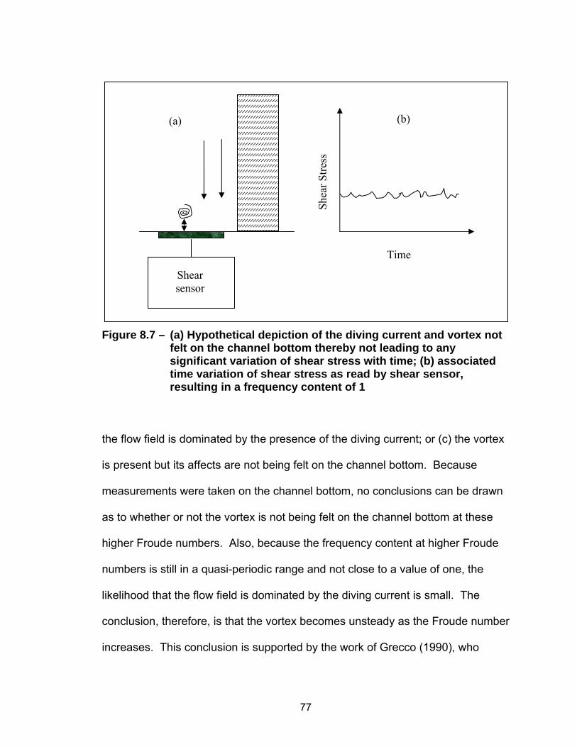
Shear sensor

(a) (b)

Time

Shea

r Stre

ss

Figure 8.7 – (a) Hypothetical depiction of the diving current and vortex not felt on the channel bottom thereby not leading to any significant variation of shear stress with time; (b) associated time variation of shear stress as read by shear sensor, resulting in a frequency content of 1

the flow field is dominated by the presence of the diving current; or (c) the vortex

is present but its affects are not being felt on the channel bottom. Because

measurements were taken on the channel bottom, no conclusions can be drawn

as to whether or not the vortex is not being felt on the channel bottom at these

higher Froude numbers. Also, because the frequency content at higher Froude

numbers is still in a quasi-periodic range and not close to a value of one, the

likelihood that the flow field is dominated by the diving current is small. The

conclusion, therefore, is that the vortex becomes unsteady as the Froude number

increases. This conclusion is supported by the work of Grecco (1990), who

77

showed that the vortex undergoes a series of stages based on approach flow

conditions, with two of the stages being simple oscillation and irregular unsteady

motion. The final stage is the complete washing away of the vortex.

To summarize, the results of the frequency content analysis show that at

lower Froude numbers, the shear measurements have an almost purely periodic

signal which can be interpreted that the vortex is present. However, as the

Froude number increases, the signal becomes quasi-periodic, leading to the

conclusion that the vortex is becoming unsteady or possibly non-existent if the

Froude number becomes high enough.

8.4.2 Probability of Exceedence

The probability that the approach shear will be exceeded can be

computed once the statistical distribution of the data string is known. A

commercial software package known as “BestFit” (Palisade Corporation 2002)

was used to analyze the data and ultimately determine the most common

statistical distribution of the data. The “BestFit” program uses several statistical

methods for determining the best distribution of the data. The results from each

method are displayed and a ranking of each distribution is given for each testing

method. In each data set, the normal distribution was shown to rank either first

or second for the best fit of the data, with approximately 90 percent of the time

being the best rank. A typical distribution is shown in Figure 8.8.

78

Normal(1.157703, 0.093602)

0.0

0.5

1.0

1.5

2.0

2.5

3.0

3.5

4.0

4.5

0.7

0.8

0.9

1.0

1.1

1.2

1.3

1.4

1.5

1.6

1.7

< >5.0% 5.0%90.0%1.004 1.312

Figure 8.8 – Histogram of a representative data set showing a typical normal distribution with corresponding mean and standard deviation

Two statistical parameters are used in order to validate a normal

distribution: skewness and Kurtosis. The skewness of a data set identifies

whether the data, after being arranged into a histogram, is more heavily weighted

to either the right (negative) or left (positive) side of the mean value. A skewness

of zero would indicate that there is the same number of data points both below

and above the mean value of the data. The skewness for each data set was

calculated and varied between -0.1 and +0.3. This range of skewness shows

that the data centers very well around the mean value, which is expected

according to the Central Limit Theorem.

The Kurtosis is another parameter which helps to identify if the data string

has a normal distribution. A Kurtosis of 3 represents a perfect normal

distribution. The Kurtosis for each data set was evaluated and showed to vary

79

from 2.6 to 3.3. This is a narrow range and therefore supports the use of normal

distribution equations for calculating exceedence probabilities.

The probability that a single shear value out of an entire data string from

an experimental data set having a normal distribution will exceed the established

threshold is based on the standard normal variant, which can be calculated using

Equation (18).

)_.(.

)_(

setdatadevst

setdatameanthreshold

τττ

φ−

= (18)

Where: Φ = Standard normal variant thresholdτ = Approach flow shear stress (Pa meanτ = Mean shear stress of data string (Pa ..devstτ = Standard deviation of data string (Pa

Once the standard normal variant is known, normal distribution tables are

used to determine the corresponding probability. The probability of exceedence

of a single measurement above the threshold, for each trial as a function of the

approach flow Froude number, was determined based on the standard normal

variant of each data set (Figure 8.9).

80

0

20

40

60

80

100

0.0 0.1 0.2 0.3 0.4 0.5

Froude number

Prob

abili

ty o

f Exc

eede

nce

(%)

Figure 8.9 - Probability that a single shear measurement from each data set will exceed the approach flow shear threshold

8.4.2.1 Analysis

Two distinct trends are observed when analyzing Figure 8.9. For Froude

numbers less than 0.33, the probability that the threshold will be exceeded is

nearly 100 percent. However, for Froude numbers greater than 0.40,

a very sharp drop-off occurs and the exceedence probability appears to be

independent of Froude number. The presence of two independent trends was

not expected so the hydraulic conditions of each trial were evaluated to

determine if a similar shallow depth phenomenon was occurring which was

observed during the unobstructed flow experiments discussed in Chapter 7. The

probabilities were plotted as a function of the depth of flow for each trial (Figure

8.10). The results show that the depth of water never drops below the 1 inch

threshold explained in Chapter 7, ruling out the possibility that the shear

81

measurements were being distorted due to increased surface tension caused by

the shallow depths. However, it is interesting to note that there is a strong

increasing correlation between depth and the probability of exceedence for

depths ranging from 1 inch to 1.5 inches. Once the depth reaches approximately

1.75 inches, the probability of exceedence stays at nearly 100 percent. In terms

of a dimensionless length ratio (depth/pier width), 1.75 inches corresponds to

approximately 0.6 (Figure 8.11).

0

20

40

60

80

100

0 0.5 1 1.5 2 2.5 3 3.5

Depth (in)

Prob

abili

ty o

f Exc

eede

nce

(%)

Figure 8.10 – Probability that a single measurement will exceed the approach flow shear threshold as a function of depth

The sudden drop off of exceedence probability at lower depths is due to

what is known as a “wide pier” effect. A wide pier is one where the pier width is

sufficiently wide compared to the water depth which in turn does not allow the

system of vortices to fully develop. The phenomenon typically is accepted to

82

occur when the length ratio of depth to pier width is less than 0.8 (Johnson

1999). The threshold ratio observed as part of this study actually is less than 0.8

and closer to 0.6. Regardless, the wide pier phenomenon appears to be present

for Froude numbers greater than 0.4 (Y/B < 0.6) and explains the presence of the

two trends observed in Figure 8.9 – at lower Froude numbers, the vortex is

completely developed and increases shear on the channel bottom nearly all of

the time; at higher Froude numbers the vortex only partially develops, and

increases of shear stress above the threshold are felt during times when a vortex

is present.

0

20

40

60

80

100

0.0 0.2 0.4 0.6 0.8 1.0 1.2

Length Ratio (Y/B)

Prob

abili

ty o

f Exc

eede

nce

(%)

Figure 8.11 – Probability of exceedence of one shear measurement exceeding the threshold as a function of the length

ratio of depth of flow to pier width, showing the presence of the wide pier phenomenon to occur at

Y/B < 0.6

83

Because the wide pier phenomenon inhibits the full formation of the vortex

system at the base of the pier, and since the intent of this work is to determine if

the vortex alone is capable of initiating scour, the following results sections will

analyze only data from Froude numbers ranging up to 0.33, where it is assumed

that the vortex system is fully developed. This will eliminate possible distortions

in analysis (and subsequent conclusions) caused by the wide pier phenomenon.

8.4.3 Percent of Time Threshold is Exceeded

The rate of threshold exceedence is a measure of how often the shear

signal exceeds the threshold in any given second. It can be found by summing

the total number of times a single measurement exceeds the threshold and then

dividing this number by duration of the entire measurement (60 seconds).

Because this value is sampling rate dependent, a better evaluator of threshold

exceedence is the percentage of time the threshold is exceeded. This

percentage can be found by dividing the rate of threshold exceedence by the

sampling rate of the measurements (200 samples per second). Table 8.1 lists

the hydraulic properties for each obstructed flow experiment with corresponding

time percentage exceedence. Figure 8.12 shows the time percentage of shear

exceedence above the threshold as a function of the approach flow Froude

number.

84

Table 8.1 – Obstructed flow hydraulic conditions with time percentage of threshold exceedence

Trial Name

Flow (lps

Depth(cm)

Velocity(cm/s) Fr # Threshold

Shear (Pa)

# Samples

above Threshold

Time %

60_7H 2.8 6.0 10.4 0.14 0.24 12000 100 60_5H 2.8 6.0 10.4 0.14 0.24 12000 100 60_4H 2.8 6.0 10.4 0.14 0.24 12000 100 60_6H 2.9 6.0 10.5 0.14 0.24 12000 100 60_8H 2.9 6.0 10.5 0.14 0.24 12000 100 70_5H 3.6 6.3 12.4 0.16 0.26 12000 100 70_4H 3.6 6.3 12.5 0.16 0.26 12000 100 70_6H 3.6 6.3 12.5 0.16 0.26 12000 100 70_7H 3.6 6.3 12.5 0.16 0.26 12000 100 70_8H 3.6 6.3 12.5 0.16 0.26 12000 100 94_5H 5.1 7.6 14.8 0.17 0.27 12000 100 94_6H 5.1 7.6 14.8 0.17 0.27 12000 100 94_4H 5.1 7.6 14.8 0.17 0.27 12000 100 94_7H 5.1 7.6 14.8 0.17 0.27 12000 100 80_6H 4.3 6.7 13.9 0.17 0.27 12000 100 80_7H 4.3 6.7 13.9 0.17 0.27 12000 100 80_4H 4.3 6.7 14.0 0.17 0.27 12000 100 80_5H 4.3 6.7 14.0 0.17 0.27 12000 100 94_5L 5.1 6.7 16.7 0.21 0.29 12000 100 90_2L 4.9 6.5 16.6 0.21 0.29 12000 100 94_4L 5.2 6.6 17.0 0.21 0.30 12000 100 94_1L 5.2 6.6 17.2 0.21 0.30 12000 100 94_3L 5.2 6.6 17.3 0.22 0.30 12000 100 90_4L 4.9 5.9 18.3 0.24 0.31 12000 100 94_2L 5.2 6.0 18.9 0.25 0.31 12000 100 90_6L 4.9 5.8 18.7 0.25 0.32 12000 100 90_1L 4.9 5.6 19.2 0.26 0.32 12000 100 90_5L 4.9 5.4 20.1 0.28 0.33 12000 100 90_3L 4.9 5.2 20.6 0.29 0.33 12000 100 85_1L 4.6 4.7 21.4 0.31 0.34 11864 99 85_2L 4.6 4.7 21.4 0.31 0.34 11927 99 85_4L 4.6 4.7 21.4 0.31 0.34 11868 99 85_5L 4.6 4.6 21.8 0.32 0.34 11915 99 85_3L 4.6 4.6 21.8 0.32 0.34 11953 100

85

010

20304050

607080

90100

0.00 0.05 0.10 0.15 0.20 0.25 0.30 0.35

Froude number

Tim

e Pe

rcen

tage

of T

hres

hold

Ex

ceed

ence

(%)

Figure 8.12 – The percentage of time that the approach flow shear stress threshold was exceeded during each experiment as a function of the approach flow Froude number

8.4.3.1 Analysis

As seen in Figure 8.12, the threshold is almost always exceeded for

Froude numbers less than 0.33 (no wide pier effect). The fact that the threshold

is always exceeded means that the vortex must always be present and felt on the

channel bottom. The reason for this is that between the two mechanisms

present in front of a pier, the vortex is the only one that can increase shear on the

channel bottom. The diving current acts in the normal direction to the channel

bottom and therefore is not capable to increasing shear (a tangential quantity).

86

8.4.4 Mean Clump Time

A group of shear measurements contained between two distinguishable

boundaries, most or all of which exceed the threshold can be considered to be a

clump (Figure 8.13). A clump of shear measurements exceeding the threshold is

much more likely than just a single burst to initiate the displacement of particles.

The time at which a clump of measurements surpasses the threshold can be

computed by summing the total number of measurements in a particular group

and then dividing by the sampling rate of the measurements (200 Hz), or through

visual inspection of a time series plot of shear vs. time for each individual trial

(Figure 8.13). The average size and time duration of each clump was

determined for each data set. The average time per clump for each data set is

plotted as a function of the approach flow Froude number in Figure 8.14.

0

0.25

0.5

8 10 12 14

Time (s)

Shea

r (Pa

)

ThresholdShear (Pa)

Clump Duration Equals 3 Seconds

Clump Duration Equals 2.3 Seconds

Average Clump Duration Equals 2.65 Seconds

Figure 8.13 –Typical data set showing how the total average duration of a clump of measurements above the threshold was obtained

87

0

0.5

1

1.5

2

2.5

3

3.5

0 0.05 0.1 0.15 0.2 0.25 0.3 0.35

Froude number

Mea

n cl

ump

dura

tion

(s)

Figure 8.14 – Average duration of all clumps from each individual experiment as a function of the approach flow Froude number

8.4.4.1 Analysis

Figure 8.14 shows a decay function of the mean duration per clump for

each data set as a function of the Froude number. At the lower Froude number

range, a duration of more than 3 seconds is achieved. A clump lasting 3

seconds is indicative of a strong primary vortex dominating the flow field before

eventually shedding downstream. As the Froude number increases to 0.33, the

mean duration decays in an exponential manner down to approximately 1

second. The transition of the decaying duration of each clump indicates that the

vortex begins to oscillate at a faster pace as the Froude number is increased.

Additionally, the average time for each clump can be considered analogous to

the duration which a particular vortex oscillates in front of the pier and over the

shear sensor before eventually shedding downstream. This would indicate that

88

the shedding frequency for Froude numbers ranging from 0.13 to 0.33 is on the

order of .33 to 1.0 cycles per second. This is in good agreement with the results

of Vautier (1972), who reported a typical shedding frequency of 0.25 to 0.50

cycles per second for each primary vortex.

8.5 Shear Amplification

The preceding sections have shown the vortex to be present nearly 100

percent of the time, if the pier is not wide compared to the depth of flow. The

question that arises is whether the vortex creates enough shear stress on the

channel bottom to initiate scour. In order to answer this question, the amount of

shear amplification between the approach flow threshold and the values

measured in front of the obstruction need to be assessed. Two parameters were

evaluated: (1) the average shear intensity amplification above the threshold

(described below), and (2) the typical peak shear amplification.

The average shear intensity is a measure of a typical or average shear value

above the approach flow threshold (Figure 8.15). Its importance stems from the

recognition that while a single burst of shear (peak shear) may cause a few

particles of sediment to transport, it is a prolonged increase of shear (average

shear intensity) which has the potential to sustain the scouring mechanism over

time. The average shear intensity can be computed based on a formula used to

calculate the average turbulence intensity, used in finding turbulence dispersion

rates. The formula is shown in Equation (19). The average shear intensity

amplification then would be equal to the average shear intensity divided by the

89

predefined shear threshold (Equation 20). The peak shear amplification is then

the “typical peak” shear (Figure 8.16) divided by the threshold (Equation 21). The

“typical peak” shear is the average of the highest peak shear values from each

clump and was used because it best represents the peak shear encountered for

each trial rather than the absolute maximum peak shear value.

threshold

avg τττ

2

int_'

= (19)

where: int_avgτ = Average shear intensity 'τ = Shear fluctuation above threshold (Pa) thresholdτ = Shear threshold (Pa)

threshold

avgampavg τ

ττ int_

int__ = (20)

where: ampavg int__τ = Average shear intensity amplification int_avgτ = Average shear intensity (Pa) thresholdτ = Approach flow shear threshold (Pa)

threshold

peaktypicalamppeak τ

ττ _

_ = (21)

where: amppeak _τ = Peak shear amplification peaktypical _τ = Typical peak shear (Pa) thresholdτ = Approach flow shear threshold (Pa)

90

peakτ

int_avgτ

thresholdτ

Time

'τ

Shea

r Stre

ss

Figure 8.15 – Hypothetical schematic of the variation of shear stress with time showing the differences between peak shear, average shear intensity, shear fluctuation above the threshold

and shear threshold

0.2

0.3

0.4

0.5

0.6

0.7

23 25 27 29

Time (s)

Shea

r (Pa

)

ThresholdShear (Pa)

τtypical peak = Average of Peaks

Figure 8.16 – Visual representation of method used to determine the typical peak shear for each trial

91

The uncertainty of each amplification was also calculated based on

rage

Equation (22) (Holman 1989). The typical peak shear amplification and ave

shear intensity amplification for each trial were found and are plotted in Figure

8.17. The amplifications with corresponding uncertainty are shown in Figures

8.18 and 8.19. The amplifications with corresponding uncertainty are listed in

Table 8.2.

2

2

22

1

1⎟⎟⎠

⎞⎜⎜⎝

⎛ Δ+⎟⎟

⎠

⎞⎜⎜⎝

⎛ Δ=Δ

xx

xx

yy (22)

where: ∆y = Uncertainty of amplification y = Amplification value

ent = 0.05 Pa t (peak or intensity) (Pa)

∆x1 = Maximum error of measurem x1 = Shear measuremen ∆x2 = Maximum error of shear threshold = 0.05 Pa x2 = Shear threshold (Pa)

0.0

1.0

2.0

3.0

4.0

5.0

0.0 0.1 0.2 0.3 0.4

Froude number

Shea

r Am

plifi

catio

n

Peak Shear Amplification

Average Shear IntensityAmplification

Figure 8.17 – Typical peak shear amplification and average shear intensity amplification of each trial as a function of the approach flow Froude number

92

0.0

1.0

2.0

3.0

4.0

5.0

0.00 0.05 0.10 0.15 0.20 0.25 0.30 0.35

Froude number

Shea

r int

ensi

ty a

mpl

ficat

ion

Figure 8.18 – Average shear intensity amplification with corresponding uncertainty

0.0

1.0

2.0

3.0

4.0

5.0

0.00 0.05 0.10 0.15 0.20 0.25 0.30 0.35

Froude number

Peak

she

ar a

mpl

ficat

ion

Figure 8.19 – Peak shear amplification with corresponding uncertainty

93

Table 8.2 – Peak shear and average intensity shear amplifications with corresponding uncertainties

Froude Number

Peak Amplification

Peak Uncertainty

Shear Intensity Amplification

Shear Intensity Uncertainty

0.14 3.9 0.9 3.7 0.8 0.14 3.9 0.8 3.7 0.8 0.14 3.8 0.8 3.7 0.8 0.14 3.8 0.8 3.7 0.8 0.14 3.8 0.8 3.7 0.8 0.16 3.2 0.7 3.5 0.7 0.16 3.2 0.7 3.5 0.7 0.16 3.2 0.7 3.5 0.7 0.16 3.2 0.7 3.5 0.7 0.16 3.2 0.7 3.5 0.7 0.17 4.0 0.8 3.6 0.7 0.17 4.0 0.8 3.6 0.7 0.17 4.0 0.8 3.6 0.7 0.17 4.0 0.8 3.6 0.7 0.17 3.5 0.7 3.0 0.6 0.17 3.5 0.7 3.0 0.6 0.17 3.4 0.7 3.0 0.6 0.17 3.5 0.7 3.0 0.6 0.21 3.8 0.7 2.9 0.5 0.21 3.4 0.6 2.7 0.5 0.21 3.6 0.6 2.8 0.5 0.21 3.5 0.6 2.7 0.5 0.22 3.7 0.6 2.8 0.5 0.24 3.1 0.5 2.3 0.4 0.25 3.0 0.5 2.3 0.4 0.25 2.9 0.5 2.2 0.4 0.26 3.1 0.5 2.2 0.4 0.28 2.7 0.4 2.0 0.3 0.29 2.8 0.5 1.9 0.3 0.31 2.5 0.4 1.7 0.3 0.31 2.8 0.4 1.6 0.3 0.31 2.6 0.4 1.6 0.3 0.32 2.6 0.4 1.6 0.3 0.32 2.5 0.4 1.6 0.3

94

8.5.1 Analysis

Peak shear amplification values vary between 2.5 (+/- 0.4) and just below

4 (+/- 0.9) with a decreasing trend as the Froude number increases. Average

shear intensity amplification values vary between 1.6 (+/- 0.3) and 3.7 (+/- 0.8)

with a decreasing trend with increasing Froude number. Interestingly, at lower

Froude numbers there are only slight variations between the peak value

amplification and the average shear intensity amplification (approximately 3.8 vs.

3.7 – Froude number = 0.14) This implies a sustained duration of the peak shear

stress values which could be attributed to a relatively slowly oscillating vortex.

These results coincide with the findings in Section 8.4.4 (Mean Clump Time),

which showed that at lower Froude numbers the duration of each clump (vortex)

was longest. Visual inspection of the shear signal also showed a flattened clump

peak at lower Froude number trials. As the Froude number increases, the

amplification values decrease at different rates, creating a greater disagreement

(approximately 2.5 vs. 1.6 – Froude number = 0.323). Visual inspection of the

shear signal with time showed a narrower peak occurring for a shorter duration of

time at higher Froude numbers, with respect to the shape and duration at lower

Froude numbers. This narrower peak with shorter duration suggests that once

the vortex is formed it quickly begins to oscillate and shed. Again this result is

corroborated by the findings in Section 8.4.4 (Mean Clump Time).

It is worth noting that each of the amplifications is below the 4 times

amplification level (disregarding uncertainty) established as the threshold by

95

which scour would be considered to initiate due to the vortex alone. This will be

discussed in greater detail in the “Discussion” section (Section 8.6).

8.5.2 Shear Amplification – Sensor Offset Adjustment

A second shear amplification analysis was performed by adjusting all of

the shear measurements by -0.2 Pa. The -0.2 Pa adjustment was made in order

to better match the theoretical prediction of shear values in an unobstructed flow

as discussed in Section (7.2.1). Equations (19-22) were used for calculating the

peak shear amplification, average shear intensity amplification and

corresponding uncertainties as in Section 8.5. Figures 8.20 and 8.21 show the

results for the average shear intensity amplification with uncertainty and peak

shear amplification with uncertainty. The results are also listed in Tables 8.3 and

8.4.

96

0.0

10.0

20.0

30.0

40.0

50.0

0.00 0.05 0.10 0.15 0.20 0.25 0.30 0.35

Froude number

Adj

uste

d av

erag

e sh

ear

inte

nsity

am

plifi

catio

n

Figure 8.20 – Adjusted average shear intensity amplification with corresponding uncertainty

0.0

10.0

20.0

30.0

40.0

50.0

60.0

0.00 0.05 0.10 0.15 0.20 0.25 0.30 0.35

Froude number

Adju

sted

pea

k sh

ear

ampl

ifica

tion

Figure 8.21 – Adjusted peak shear amplification with corresponding uncertainty

97

Table 8.3 – Adjusted threshold, peak, and average intensity shear values

Froude number

Adjusted threshold

Adjusted peak shear

Adjusted average shear intensity

0.14 0.04 0.72 0.68 0.14 0.04 0.71 0.68 0.14 0.04 0.71 0.68 0.14 0.04 0.71 0.68 0.14 0.04 0.70 0.68 0.16 0.06 0.63 0.60 0.16 0.06 0.63 0.60 0.16 0.06 0.64 0.61 0.16 0.06 0.64 0.61 0.16 0.06 0.63 0.58 0.17 0.07 0.87 0.75 0.17 0.07 0.86 0.76 0.17 0.07 0.87 0.77 0.17 0.07 0.87 0.76 0.17 0.07 0.75 0.60 0.17 0.07 0.75 0.60 0.17 0.07 0.73 0.60 0.17 0.07 0.75 0.60 0.21 0.09 0.92 0.65 0.21 0.09 0.80 0.60 0.21 0.10 0.85 0.64 0.21 0.10 0.84 0.61 0.22 0.10 0.91 0.63 0.24 0.11 0.77 0.53 0.25 0.11 0.73 0.52 0.25 0.12 0.73 0.50 0.26 0.12 0.78 0.49 0.28 0.13 0.67 0.44 0.29 0.13 0.73 0.43 0.31 0.14 0.64 0.36 0.31 0.14 0.75 0.35 0.31 0.14 0.66 0.35 0.32 0.14 0.68 0.35 0.32 0.14 0.66 0.35

98

Table 8.4 – Adjusted peak shear and average intensity shear amplification with corresponding uncertainty

Froude number

Adjusted Peak Amplification

Adjusted peak uncertainty

Adjusted Shear Intensity

Amplification

Adjusted Shear Intensity

Uncertainty 0.14 20.1 28.2 19.1 26.8 0.14 19.7 27.3 18.8 26.1 0.14 19.5 26.9 18.7 25.7 0.14 19.1 25.9 18.4 24.9 0.14 19.0 25.7 18.4 24.9 0.16 11.0 9.7 10.1 8.7 0.16 11.0 9.6 10.0 8.5 0.16 11.1 9.6 10.0 8.4 0.16 11.0 9.6 10.0 8.5 0.16 11.0 9.6 10.0 8.4 0.17 12.8 9.4 11.0 8.1 0.17 12.6 9.3 11.1 8.1 0.17 12.8 9.4 11.2 8.2 0.17 12.7 9.3 11.1 8.1 0.17 10.9 7.9 8.6 6.3 0.17 10.9 7.9 8.7 6.3 0.17 10.5 7.6 8.6 6.3 0.17 10.9 7.9 8.6 6.3 0.21 9.9 5.4 7.0 3.8 0.21 8.5 4.5 6.4 3.4 0.21 8.9 4.7 6.7 3.5 0.21 8.6 4.4 6.2 3.2 0.22 9.2 4.7 6.4 3.3 0.24 6.9 3.1 4.7 2.2 0.25 6.4 2.9 4.5 2.0 0.25 6.3 2.8 4.4 1.9 0.26 6.5 2.8 4.1 1.8 0.28 5.3 2.1 3.5 1.4 0.29 5.7 2.2 3.3 1.3 0.31 4.7 1.8 2.6 1.0 0.31 5.5 2.1 2.6 1.0 0.31 4.8 1.8 2.6 1.0 0.32 4.9 1.8 2.5 1.0 0.32 4.7 1.8 2.5 1.0

99

8.5.2.1 Analysis

Peak shear amplification values vary between 20.1 (+/- 28.2) and 4.7 (+/-

1.8) with a decreasing trend as the Froude number increases. Average shear

intensity amplification values vary between 19.1 (+/- 26.8) and 2.5 (+/- 1.0) with a

decreasing trend with increasing Froude number. Just as in the case of there

being no offset adjustment, the peak value amplification and the average shear

intensity amplification are relatively close to one another at lower Froude

numbers (approximately 20.1 vs. 19.1 – Froude number = 0.14). There is a more

pronounced decrease of shear amplification with increasing Froude number in

the adjusted shear value situation as opposed to the non-adjusted case.

Interestingly, all of the adjusted peak shear amplification values are above the 4

times amplification criteria set to indicate whether the vortex alone has the

potential to solely initiate scour, which is contrary to the results obtained without

the offset adjustment.

8.5.3 Comparison to Historical Results

8.5.3.1 Melville and Raudkivi (1977)

Melville and Raudkivi (1977) performed an extensive study of the flow

characteristics in the vicinity of vertical obstructions. As part of their investigation

they ascertained a shear stress distribution in front of and around a pier at an

elevation of 2 mm. The flow characteristics of their study were as follows: mean

velocity = 0.25 m/s, uniform flow depth = 0.15 m, Froude number = 0.206, and

bed slope = 0.0001. They also reported an approach flow shear velocity equal to

100

.0121 m/s calculated from Equation (23). Using this value of shear velocity, the

approach flow shear stress was calculated according to Equation (10) and found

to equal 0.146 Pa.

ooSgyu =* (23)

where: u* = Shear velocity (m/s) g = Acceleration of gravity = 9.8 m/s2

yo = Uniform flow depth (m) So = Bed slope (m/m)

Mean shear stress values were calculated at various points in front of and

around the pier by Melville and Raudkivi (1977) using Equation (24):

yuK

ΔΔ

=τ (24)

where: τ = Mean bed shear stress (Pa) K = Calibration constant obtained by comparing estimated shear values from Equation (23) with those obtained from the slope of the logarithmic velocity profile of the approach flow = 2 uΔ = Local mean velocity at 2 mm from bed = 2 mm yΔ

Melville and Raudkivi (1977) report a decreasing shear stress distribution

in front of the pier in the flow direction as the pier is approached. Shear stress

values measured ranged from 0.04 Pa to 0.07 Pa, which can be normalized to

the approach flow shear stress as 0.27 to 0.47 magnifications. These values are

less than the approach flow shear stress and substantially different from the

101

values recorded as part of this work (approximately 3.5 peak shear magnification

factor (non-offset adjustment) at a Froude number equal to 0.21). It was this

measured reduction in shear stress that lead Melville and Raudkivi to conclude

that scour is caused by the diving current reflecting off the pier and not an

increase in shear stress caused by the vortex.

The method of shear stress measurement in front of the pier which

Melville and Raudkivi employed is not adequate for such a conclusion. Their

method involved using what is essentially Newton’s law of viscosity based on an

average velocity reading. This method has associated inherent errors. To begin,

their method does not result in a shear stress calculation on the channel bottom;

it was taken as 2 mm above the channel bottom as indicated earlier.

Additionally, the method does not account for the turbulent stresses due to the

velocity fluctuations of the flow field which might actually dominate the total shear

stress value at this location due to the vortex. Finally, and most importantly, this

method assumes that the flow field in front of a pier is constant.

Several investigators, as well as the results from this work, show that this

is not the case, as the flow field is constantly changing due to the oscillatory

nature of the vortex. Recording an average velocity from an oscillatory

mechanism and using this value in a shear stress prediction should produce a

diminished shear stress, because on average the velocity would be close to zero

due to the velocity profile fluctuating between a positive and negative value due

to the motion of the vortex (Figure 8.22). Analysis of the shear stress predictions

associated with the greatest change in velocity gradient, instead of the average

102

velocity gradient, would probably be a better indicator of the shear stress values

which might lead to scour and could possibly lead to a better comparison to the

shear stress amplifications found in this work.

Figure 8.22 – Developing velocity profile due to the formation and oscillation of a vortex

8.5.3.2 Mendoza-Cabrales (1993)

Mendoza-Cabrales developed a k-ε closure model (where k is kinetic

energy and ε is the energy dissipation rate) in an attempt to ascertain shear

stress values on a flat bed around a cylinder. He simulated the experimental

setup of Melville and Raudkivi (1977) for comparative purposes. His model

predicted shear stress amplification values that were at the lower end of the

values reported by Melville and Raudkivi (.27). However, Mendoza-Cabrales

concluded that his model was not suitable for shear stress determination in front

of an obstruction because, like Melville and Raudivi’s work, it only reports an

average shear stress and “the k- ε closure model should be expected to yield

103

only an adequate description of the bulk flow, not the detailed resolution of the

changing stresses” (Mendoza-Cabrales 1993, p 904).

8.5.3.3 Ahmed and Rajaratnam (1998)

Ahmed and Rajaratnam (1998) used a series of two three-tube Yaw

probes as Preston probes in an attempt to measure bed shear stresses. The

Preston probe gives a velocity profile of the flow, from which Newton’s law of

viscosity can be used to predict shear stresses. Ahmed and Rajaratnam (1998)

do not give exact heights at which the measurements were taken, but claim the

measurements are approximately “on the bed.” Additionally, they do not state

the nature of the velocities used for shear stress prediction (average - similar to

Melville and Raudkivi’s (1977) technique, or extremes). Measurements were

taken both in an unobstructed and obstructed flow. Two experiments were

completed using a smooth bed: Experiment 1 - mean velocity = 0.29 m/s,

uniform depth = 0.19 m, Froude number = 0.22, approach flow shear stress =

0.18 Pa; Experiment 2 – mean velocity = 0.38 m/s, uniform depth = 0.14 m,

Froude number = 0.33, approach flow shear stress = 0.32 Pa. The results of the

shear stress measurements in front of the pier then were normalized by dividing

by the approach flow (unobstructed) shear stress. The normalized shear

stresses were plotted as a function of the distance upstream of the pier. Their

results show that at the immediate base of the pier, the shear can be amplified by

as much as six times the approach flow shear; within two pier diameters

upstream, the shear stress decays but is in the range of 1.5 - 4 times the

104

approach flow shear value. Past two pier diameters the shear gradually drops off

to the approach flow shear value. These results suggest that Ahmed and

Rajaratnam (1998) did not use average velocities as part of their analysis, but

rather a group of velocities which corresponded to the highest gradient of

measurements. Their results at the base of the pier (within two pier widths

upstream) compare favorably with the peak and average shear intensity

amplifications (1.5–4) found in this work (Section 8.5).

8.5.3.4 – Ali and Karim (2002)

Ali and Karim (2002) used the FLUENT CFD model in an attempt to study

the flow field around a cylinder on both a flat bed and in a scour hole. A 45 x 28

non-uniform grid was mapped in the domain cross-section which had limits of

three pier diameter widths upstream and six pier diameter widths downstream.

Neither the depth of flow nor approach Froude number were given, but a mean

velocity of 0.067m/s was used for simulation. The results of the flat bed

simulation show an almost complete absence of shear stress at the base of the

upstream side of the pier. A shear magnification (shear at pier / approach flow

shear) ranging from 0.007 to 0.021 is shown on the bed within one pier diameter

upstream of the pier. These results suggest the absence of any vortex upstream

of the pier. A visual illustration of the flow field shows this to be true, as the area

immediately upstream of the pier is dominated by a diving current only.

Downstream visuals, however, show the shedding of several vortices. The lack

of the vortex at the upstream side of the pier being simulated with the model,

105

which has been shown to exist in numerous studies, makes the results of this

study unsuitable for comparison.

8.5.3.5 Jones (2002)

Jones (2002) performed experiments using PIV (Particle Image

Velocimetry) in order to ascertain the flow field in front of a pier. Based on the

flow field, he was able to determine the shear stress averaged over a period of

time on the channel bed using Newton’s law of viscosity (Equation 25) and the

shear stress for several millimeters above the channel bed using a combination

of laminar (Equation (25)) and turbulent stresses (Equation (26)).

dydu

lam μτ = (25)

Where: τlam = Laminar shear stress (Pa) μ = Absolute viscosity (N s/m2)

dydu = Gradient of velocity profile

''vutur ρτ = (26)

Where: turτ = Turbulent shear stress (Pa) ρ = Density of water = 1000 (kg/m3) u’ = Velocity fluctuation in x-direction (m/s) v’ = Velocity fluctuation in y-direction (m/s)

From a time average analysis of his PIV recordings, Jones (2002) saw the

presence of both a diving current and a vortex upstream of the pier. The shear

stress calculated on the bed at the location of the diving current (at the

106

intersection of the pier and channel bed) was negligible, but under the vortex

(location was within one pier diameter upstream) the shear stress was amplified

by approximately six times the approach flow value.

While Jones’ results do not incorporate the oscillatory motion of the vortex,

they do present a shear stress which can be expected to be generated under a

stationary vortex close to the channel bottom (0.3 mm). A stationary vortex is

likely to yield the maximum shear value, when viewing the time-shear signature

of an oscillatory vortex. Therefore, Jones’ results are comparable to the peak

shear amplification results of this study.

The experimental flow conditions were not presented in the paper but

Jones (2002, p 148) states that there is “an inherent assumption that the ratio of

shear stresses holds for a wide range of approach flow velocities.” Therefore, his

results cannot be compared to the results of this study at any particular Froude

number, but only over the entire spectrum. Jones’ results in general are

approximately 50 to 100 percent higher than the peak shear amplification ratios

calculated in this study. One possible reason for the lack of agreement is that

Jones predicted the shear stress under the vortex by ascertaining the velocity

profile through the vortex and then extrapolating the slope of the velocity curve

from the lowest measured point (0.3 mm) to the channel bottom, from which he

used Newton’s law of viscosity to determine the shear stress. This method is

only viable if the final few points on the velocity curve, which depict its slope, are

within the laminar sublayer of the flow where the velocity change is assumed to

be linear. While 0.3 mm is very close to the boundary, rough approximations of

107

the boundary layer height for the presumed flow conditions (based on personal

observation of experimental setup - Froude number = 0.2) result in a boundary

layer thickness of about 0.3 – 0.4 mm, meaning that the final few points used to

determine the slope of the velocity profile may have been outside the laminar

sublayer. Jones realized the potential errors associated with this type of

prediction and cautioned that the manner in which the velocity profile was

extracted to the channel bottom could have resulted in boundary shear

amplification predictions ranging from less than 1 up to 95. A more detailed

study using PIV, generating data closer to the boundary (say 0.1 mm) may

produce results quantitatively similar to the ones found in this study. Finally,

while Jones’ (2002) results do not compare favorably to the ones found in this

study, they are on the same order of magnitude and suggest that using PIV may

be a viable option for shear stress determination under a stationary vortex.

8.6 Discussion of Results

Overall, the results of the previous analyses show the continuous

presence of a vortex system upstream of an obstruction. The results from the

frequency content analysis show the measurements to be quasi-periodic, which

suggests that one vortex did not stay in front of the pier for the entire length of

each measurement and that after a certain duration (dependent on Froude

number) the vortex shed. A new vortex is suspected to have developed before

the original one shed based on the fact that the approach flow shear stress was

always exceeded, and the underlying assumption that only the vortex has the

108

ability to increase the shear stress upstream of a pier. The duration that each

vortex stayed in front of the pier before eventually shedding downstream was

found to range between 1 and 3 seconds, with a faster shedding frequency

associated with higher Froude numbers, suggesting that at lower Froude

numbers, a single vortex may dominate the flow field for relatively longer periods

of time.

The results of the peak shear amplification analysis are rather contrary

when comparing the adjusted shear values to the unadjusted shear values.

Peak amplifications vary from 3.9 for the unadjusted analysis to 20.1 for the

adjusted analysis. These differences in amplification can lead to drastically

different conclusions when trying to ascertain if the vortex increasing shear has

the potential to solely initiate scour. It is the authors’ opinion that the unadjusted

shear amplification results better represent a more accurate assessment of the

shear amplification results. This is based on the fact that the mechanics of the

flow field are quite different between the unobstructed and obstructed flow

situations, and therefore does not seem legitimate to adjust the obstructed flow

results to coincide with a theoretical prediction of an entirely different mechanism.

Additionally, the unadjusted peak shear amplifications have a better agreement

with shear amplifications measured by other investigators such as Ahmed and

Rajaratnam (1998) and Jones (2002), suggesting the unadjusted values are

more proper.

The question of whether the vortex increases shear enough to solely

initiate scour is now addressed. Recall that several investigators witnessed the

109

initiation of scour at the base of a pier once the approach flow shear velocity

reaches half of the critical velocity necessary for a particular sediment to

transport. Based on this observation and Equation (10), the original hypothesis

was formulated that the increase of shear stress at the base of a pier is at least

four times the approach flow value, and that the increase is responsible for

initiating scour. The peak shear amplification results show this condition is

approached (and possibly exceeded based on the maximum uncertainty of the

ratio) at the lower range of Froude numbers tested as part of this study, with

peak shear amplifications being as high as 3.9 (+/- 0.9). Additionally, there is an

increasing trend of peak shear amplification as the Froude number decreases,

implying that if tests had been conducted at Froude numbers smaller than 0.13,

the conditions of the hypothesis may have been met based on measurement

alone (without uncertainty analysis). As it is, however, the hypothesis condition

was not met and the peak shear amplification (disregarding uncertainty) never

exceeded the 4 times amplification condition. Interestingly, the amplification

value did not stay at a constant level (which has been assumed by various

investigators), but instead dropped to as low as 2.5 (+/- 0.4) at the highest

Froude numbers tested; the trend suggests that this value would have continued

to diminish with increasing Froude number. An analysis of the flow field

presented by Raudkivi (1986) and Ahmed and Rajaratnam (1998) can be used to

give one possible explanation for the decreasing peak shear amplification with

increasing Froude number.

110

Ahmed and Rajaratnam (1998) conducted experiments at a Froude

number of approximately 0.2 and found that the diving current reflecting off the

face of a pier reaches approximately 35 percent of the mean approach flow

velocity. Raudkivi (1986) conducted experiments at Froude numbers in the

range of 0.5 to 0.6 and found the diving current reached approximately 80

percent of the mean approach flow velocity. Comparison of these results shows

that as the approach flow velocity (Froude number) increases, the diving current

velocity also increases. An increase in diving current velocity is thought to have

the potential to create larger disturbances in the flow field due to its greater

impact on the channel bottom possibly making the formation and effectiveness of

the vortex more difficult. This suggestion is corroborated by the work of Eckerle

and Awad (1991), who showed that if the approach flow velocity (Pier Reynolds

number) becomes too great that the vortex system will not form at all, but the

diving current still will exist.

Therefore, analysis of these three studies as well as the results from this

study suggest that the initiation of scour at the upstream face of a pier and the

mechanism which causes it may be entirely dependent on approach flow

conditions, where scour created in flows which are deep and slow moving (low

Froude number) may be initiated and controlled by the shear stress under the

vortex, and scour in flows which are shallow and fast (high Froude number) may

be initiated by the diving current reflecting off the pier. A further more detailed

study involving measurements of both the shear stress under the vortex and the

diving current velocity, in a movable bed, is warranted before a definitive final

111

conclusion can be made about this shifting of controlling mechanism based on

approach flow conditions. As for this study in regards to its purpose, the results

indicate that scour is most likely not caused by an increase in shear stress alone.

112

CHAPTER 9

CONCLUSIONS

9.1 Unobstructed Flow/Shear Sensor

A shear measuring device has been designed and implemented which

uses a series of four strain gages to measure the amount of tangential force

occurring over a flat plate mounted flush to a channel bottom. The force, leading

to a displacement of the measuring plate, is calibrated to yield an applied shear

stress over the surface. This device was used to ascertain a relationship

between a uniform flow Froude number and an applied shear stress. A total of

69 experiments were completed.

The results from the sensor were compared to two theoretical equations.

Each of these equations stems from different assumptions and is independent in

the derivation. The equations produced similar results to one another, but in

general under-predicted the values measured from the shear sensor by an

average of 0.2 Pa. The trends obtained from both equations and the measuring

sensor were agreeable, implying that the sensor was in working order.

Additionally, the sensor showed a rapid increase in shear once the depth of flow

dropped below 1 inch. This increase was expected based on the work of Ettema

(2000), who stated that once the depth flow falls beneath approximately 1 inch,

additional forces due to surface tension (which normally are not present) can

begin to dominate. Overall, the sensor is considered to be in working order and

a viable device which can be used for boundary shear stress measurements.

113

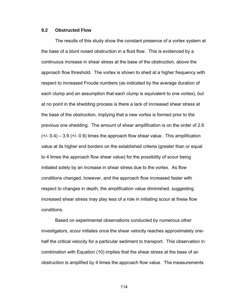
9.2 Obstructed Flow

The results of this study show the constant presence of a vortex system at

the base of a blunt nosed obstruction in a fluid flow. This is evidenced by a

continuous increase in shear stress at the base of the obstruction, above the

approach flow threshold. The vortex is shown to shed at a higher frequency with

respect to increased Froude numbers (as indicated by the average duration of

each clump and an assumption that each clump is equivalent to one vortex), but

at no point in the shedding process is there a lack of increased shear stress at

the base of the obstruction, implying that a new vortex is formed prior to the

previous one shedding. The amount of shear amplification is on the order of 2.6

(+/- 0.4) – 3.9 (+/- 0.9) times the approach flow shear value. This amplification

value at its higher end borders on the established criteria (greater than or equal

to 4 times the approach flow shear value) for the possibility of scour being

initiated solely by an increase in shear stress due to the vortex. As flow

conditions changed, however, and the approach flow increased faster with

respect to changes in depth, the amplification value diminished, suggesting

increased shear stress may play less of a role in initiating scour at these flow

conditions.

Based on experimental observations conducted by numerous other

investigators, scour initiates once the shear velocity reaches approximately one-

half the critical velocity for a particular sediment to transport. This observation in

combination with Equation (10) implies that the shear stress at the base of an

obstruction is amplified by 4 times the approach flow value. The measurements

114

conducted as part of this study, however, show this not to be the case.

Therefore, it is concluded that scour is most likely not caused by increases in

shear stress alone. The more likely scenario is that scour is caused by a

combination of both a reduced pressure field around the particles caused by the

generation of a diving current impacting the channel bed normally, and an

increase in shear stress caused by the formation of a vortex system.

Based on the results of this work and conclusions mentioned previously,

the question still remains: “Should the current scour equations be modified to

include a shear stress parameter?” The simplest answer is YES, due to the fact

that there are definite increases in shear stress; however, it may not be possible

due to the following reason. As it is, in a non-uniform flow, shear stress

predictions on a channel bottom are adequate at best. This is because shear

stress is a function of multiple variables which are constantly changing from one

section to the next in a natural environment due to irregularities along the

channel bottom both laterally and in the flow direction. Therefore, the prediction

of an accurate approach flow shear stress and a corresponding shear

amplification value at the base of a pier is not obtained easily. Additionally,

simply adding a shear stress variable to the current scour equations still does not

account for the inherent presence of the diving current and its effect on initiating

scour and its role in determining an ultimate scour depth.

Possibly a better solution would be to experimentally determine the overall

relationship between approach flow conditions, the diving current reflecting off

the pier, the increase in shear stress due to the vortex, and the associated effect

115

on a maximum depth of scour. Then, with this detailed knowledge of all four

factors, methods for predicting scour depths could be developed, in lieu of just

ascertaining a regression equation based on flow conditions and a scour depth,

as is typically done. Until researchers gain a better understanding of each of the

above-named mechanisms and their relationship to one another, scour

predictions based on current methods will be adequate at best.

As a final note, it is interesting to observe the development of the wide pier

phenomenon. Although this effect generally has been accepted to occur once

the ratio of depth of flow to pier width falls below 0.8, this work has shown it to

occur for ratios less than 0.6. More experimental work in this area is warranted

to quantify an exact value at which this phenomenon occurs.

9.3 Engineering Significance / Recommendations

This work can prove to be very beneficial to the practicing engineering

community. Much research has been completed and subsequent debates have

arisen about the scouring process at the base of blunt-nosed piers. The results

of this research show that the scouring process is a complex phenomenon which

is driven by two components. With this knowledge, the results can be used to

engineer new and better designs of piers, their foundations, and corresponding

protective structures (flow arrestors, riprap, etc.). The new designs would have

to incorporate devices which can be used to abolish the downflow component.

Additionally, appropriate sized riprap or other shear protective measures would

have to be implemented based on the results of the peak shear amplification

116

analysis. It is recommended that these protective measures be based on an

increase in shear of at least four times the undisturbed value.

Finally, the results of this work can prove to be paramount in the current

research being conducted on scour of cohesive soils at the base of piers. Most

of the research is centered on finding an exact shear amplification factor as well

as a time rate of scour factor. The overall findings of this research show a

functional relationship of shear amplification vs. Froude number. Additionally, the

results of each trial of this research deliver a relationship of shear vs. time at

various Froude numbers. An analysis of the data from each trial can be very

helpful in quantifying the frequency with which the shear exceeds a given

threshold, and therefore help in the determination of an appropriate decay

function depicting a time rate of scour for various soil types.

9.4 Future Work

While the completion of this work has provided valuable insight into the

mechanism which leads to the initiation of scour, much more research could be

completed in order to fully maximize the resourcefulness of the sensor. The

following tasks are recommended:

• Experiments which include the simulation of various bed roughnesses

should be completed both with and without the presence of the pier to

determine what affect bed roughness has on the amplification of shear in

front of an obstruction.

117

• Experiments should be completed using both different sized and different

shaped piers in order to verify whether either of these two parameters has

a significant impact on the results of this research.

• Experiments should be conducted which include mobile sediment to

determine at which flow conditions and corresponding shear stress does

scour actually initiate.

• Experiments should be conducted simultaneously using both the shear

sensor to quantify shear values, and a visual method such as PIV, to

quantify the flow field and associated magnitude of the diving current, in

order to determine a relationship between these two mechanisms and the

relative effect each has on initiating scour at various flow conditions.

• More experiments should be conducted at shallow depths to better

quantify an exact depth of flow to pier width ratio which the vortex has

trouble forming, leading to the generation of a wide pier situation.

118

REFERENCES

Abed, L.M., 1991, “Local Scour around Bridge Piers in Pressure Flow,” Dissertation, Civil Engineering Dept., Colorado State University, Fort Collins, CO.

Abed, L., and Gasser, M., 1993, “Model Study of Local Scour Downstream

Bridge Piers,” ASCE Hydraulic Engineering, Proc. 1993 National Conference, 1738-1743.

Ahmed, F., and Rajaratnam, N., 1998, “Flow Around Bridge Piers,” Journal of Hydraulic Engineering, Vol. 124, No. 3, 288-300. Ali, K.H.M., and Karim, O.A., 2002, “Simulation of Flow Around Piers,” Journal of Hydraulic Research, Vol. 40, No. 2, 161-174. Ali, K.H.M., and Lim, S.Y., 1986, “Local Scour Caused by Submerged Wall-Jets,” Proceedings of the Institution of Civil Engineers, London, England, Vol. 81, No. 2, 607-645. Annandale, G.W., 1999, “Calculation of Pier Scour using the Erodibility Index

Method,” Draft notes for a short course presented to the Maryland State Highway Administration.

Ansari, S.A., et al., 2002, “Influence of Cohesion on Scour Around Bridge Piers,” Journal of Hydraulic Research, Vol. 40, No. 6, 717-729. Baker, C.J., 1980, “Theoretical Approach to Prediction of Local Scour Around Bridge Piers,” Journal of Hydraulic Research, Vol. 18, No. 1, 1-12. Breusars, et al., 1977, “Local Scour Around Cylindrical Piers,” Journal of

Hydraulic Research, Vol. 15, No. 3, 211-252. Briaud, J.L., et al., 1999, “SRICOS: Prediction of Scour Rate in Cohesive Soils at Bridge Piers,” Journal of Geotechnical and Geoenvironmental Engineering, Vol. 125, 237-246. Brice, J.C., and Blodgett, J.C., 1978, “Countermeasures for Hydraulic Problems at Bridges,” Vol. 1 and 2, FHWA/RD-78-162&163, Federal Highway

Administration, U.S. Department of Transportation, Washington D.C. Carstens, M.R., 1966, “Similarity Laws for Localized Scour,” Journal of Hydraulic Engineering, Vol. 92, No. 3, 13-36. Chabert, J., and Engeldinger, P., 1956, Etude des Affonillements Author des Piles des Ponts, Laboratoire National d’Hydraulique, Chatoe, France.

119

Chaudhry, M.H., 1993, “Open-Channel Flow,” Published by Prentice-Hall, Inc., 263.

Dargahi, B., 1987, “Flow Field and Local Scouring Around a Cylinder,” Bulletin No. 37, R. Inst. Tech. Hydr. Lab, Stockholm, Sweden. Dargahi, B., 1989, “The Turbulent Flow Field Around a Circular Cylinder,”

Experiments in Fluids, Vol. 8, 1-12. Dargahi, B., 1990, “Controlling Mechanism of Local Scouring,” Journal of

Hydraulic Engineering, Vol. 116, No. 10, 1197-1214. Davis, S.R., 1984, “Case Histories of Scour Problems at Bridges,” Transportation

Research Record 950, Second Bridge Engineering Conference, Vol. 2, Transportation Research Board, Washington D.C.

Dey, S., et al., 1995, “Clear Water Scour at Circular Piers,” Journal of Hydraulic Engineering, Vol. 121, No. 12, 869-876. Dou, X., 1997, “Numerical Simulation of Three-Dimensional Flow Field and Local

Scour at Bridge Crossings,” Dissertation, Computational Hydroscience Engineering, University of Mississippi, University, MS.

Eckerle, W.A., and Awad, J.K., 1991, “Effect of Freestream Velocity on the Three-Dimensional Separated Flow Region in Front of a Cylinder,” Journal

of Fluid Engineering, Vol. 113, 37-44. Edge, B.L., et al., 1998, “Determination of Velocity in Estuary for Bridge Scour Computations,” Journal of Hydraulic Engineering, Vol. 124, No. 6, 619-628. Ermshaus, R., 1985, “Hot Film Anemometry,” Institute of Hydromechanics, University of Karlsruhe, Germany, Seminar Notes (October 4-6). Ettema, R., 1980, “Scour at Bridge Piers,” Rep. No. 216, School of Engineering, University of Auckland, New Zealand. Ettema, R., 2000, “Hydraulic Modeling – Concepts and Practice,” ASCE Manuals and Reports on Engineering Practice No. 97, Published by American

Society of Civil Engineers, Reston, VA, 41, 63 Ettema, R., et al., 1998, “Scale Effect in Pier-Scour Experiments,” Journal of Hydraulic Engineering, Vol. 124, No. 6, 639-642.

120

Froehlich, D.C., 1988, “Analysis of On-site Measurements of Scour at Piers,” Proceedings of the 1988 National Conference on Hydraulic Engineering, Colorado Springs, Colorado, August 15-19, 1988, American Society of Civil Engineers, New York, NY, 826-831.

Froehlich, D.C., 1996, “Bridge Hydraulic and Scour Analysis using FESWMS-

2DH,” ASCE, North American Water and Environmental Congress, Washington D.C.

Gradowcyzk, M.H., 1968, “Localized Scour in Erodible Bed Channels,” Journal of

Hydraulic Research, Vol. 6, No. 4, 289-334. Graf, W.H., and Istiarto, I., 2002, “Flow Pattern in the Scour Hole around a

Cylinder,” Journal of Hydraulic Research, Vol. 40, No. 1, 13-20. Grecco, J.J., 1990 “The Flow Structure in the Vicinity of a Cylinder-Flat Plate Junction: Flow Regimes, Periodicity, and Vortex Interactions,” Masters

Thesis, Department of Civil Engineering, Lehigh University, Bethlehem, PA.

Hancu, S., 1971, “Sur le Calcul des Affouillements Locaus Dams la Zone des Piles de Ponts,” Proc. 14th IAHR Cong., Vol. 3, 299-313. Holman, J.P., 1989, “Experimental Methods for Engineers”, 5th edition, Published by McGraw-Hill, Inc., p. 42 Jain, S.C., 1981, “Maximum Clear-Water Scour Around Circular Piers,” Journal of Hydraulic Engineering, Vol. 107, No. 5, 611-626. Jain, S.C., and Fischer, E.E., 1980, “Scour Around Bridge Piers at High Flow Velocities,” Journal of Hydraulic Engineering, Vol. 106, No. 11, 1827-1841. Johnson, P.A., 1992, “Reliability–Based Pier Scour Engineering,” Journal of Hydraulic Engineering, Vol. 118, No. 10, 1344-1357. Johnson, P.A., 1995, “Comparison of Pier-Scour Equations using Field Data,” Journal of Hydraulic Engineering, Vol. 121, No. 8, 626-629. Johnson, P.A., 1999, “Scour at Wide Piers Relative to Flow Depth,” Compendium of ASCE Conference Papers Edited by E.V. Richardson and P.F. Lagasse, 280-287 Johnson, P.A., and Ayyub, B.M., 1992, “Assessing Time-Variant Bridge

Reliability Due to Pier Scour,” Journal of Hydraulic Engineering, Vol. 118, No. 6, 887-903.

121

Johnson, P.A., and Jones, S., 1992, “Shear Stress at Base of Bridge Pier,” Transportation Research Record No. 1350, Transportation Research Board, 14-18.

Johnson, P.A., and Jones, S., 1993, “Merging Laboratory and Field Data in

Bridge Scour,” Journal of Hydraulic Engineering, Vol. 119, No. 10, 1176- 1181.

Jones, S., 1993, “Preliminary Studies on Pressure Flow Scour,” ASCE Hydraulic Engineering, Proc. 1993 National Conference, 916-921. Jones, S., 2002, “Indirect Methods of Measuring Shear Stress in the Bottom of a Scour Hole,” First International Conference on Scour of Foundations, Conference Proceedings, 140-155. Kandasamy, J.K., and Melville, B.W., 1998, “Maximum Local Scour Depth at

Bridge Piers and Abutments,” Journal of Hydraulic Research, Vol. 36, No. 2, 183-198.

Karim, O.A., and Ali, K.H.M., 2000, “Prediction of Flow Patterns in Local Scour

Holes Caused by Turbulent Water Jets,” Journal of Hydraulic Research, Vol. 38, No. 4, 279-288.

Kirkgoz, M.S., and Ardichoglu, M., 1997, “Velocity Profiles of Developing and Developed Open Channel Flow,” Journal of Hydraulic Engineering, Vol. 123, No. 12, 1099-1105. Kothyari, U.C., et al., 1992, “Temporal Variation of Scour Around Circular Bridge

Piers,” Journal of Hydraulic Engineering, Vol. 118, No. 8, 1091-1106. Kothyari, U.C., et al., 1993, “Live Bed Scour Around Cylindrical Bridge Piers,” Journal of Hydraulic Research, Vol. 30, No. 5, 701-715. Kundu, P.K., 1990, “Fluid Mechanics,” Oceanographic Center, Nova University,

Dania, FL, Academic Press, Inc., 452. Larras, J., 1963, “Profondeurs Maximales d’Erosion Des Fonds Mobiles Autour Des Piles En Rivere,” Ann. Ponts et Chaussees, Vol. 133, No. 4, 411-

424. Laursen, E.M., 1960, “Scour at Bridge Crossings,” Journal of Hydraulic

Engineering, Vol. 86, No. 2, 39-54. Laursen, E.M., 1963, “An Analysis of Relief Bridge Scour,” Journal of Hydraulic Engineering, Vol. 89, No. 3, 93-118.

122

Laursen, E.M., and Toch, A., 1956, “Scour Around Bridge Piers and Abutments,” Bulletin No. 4, Iowa Highway Research Board, Ames, IA. Lemmin, U., and Rolland, T., 1997, “Acoustic Velocity Profiler for Laboratory and Field Studies,” Journal of Hydraulic Engineering, Vol. 123, No. 12, 1089-1098. Li, Y., et al., 2002, “Shear Stress Approach to Pier Scour Predictions,” First International Conference on Scour of Foundations, Conference

Proceedings, 140-155. Maull, D.J., and Young, R.A., 1973, “Vortex Shedding from Bluff Bodies in a

Shear Flow,” Journal of Fluid Mechanics, Vol. 60, Part 2, 401-409. Melville, B.W., 1975, “Local Scour at Bridge Sites,” Report No. 117, University of Auckland, Auckland, New Zealand. Melville, B.W., and Raudkivi, A.J., 1977, “Flow Characteristics in Local Scour at

Bridge Piers,” Journal of Hydraulic Research, Vol. 15, No. 4, 373- 380.

Melville, B.W., and Sutherland, A.J., 1988, “Design Method for Local Scour at

Bridge Piers,” Journal of Hydraulic Engineering, Vol. 114, No. 10, 1210- 1226.

Mendoza-Cabrales, C., 1993, “Computation of Flow Past a Cylinder Mounted on a Flat Plate,” ASCE Hydraulic Engineering, Proc. 1993 National Conference, 899-904. Muller, G., et al., 2001, “Mapping of Bridge Pier Scour with Projection Moire,” Journal of Hydraulic Research, Vol. 39, No. 5, 1-7. National Transportation Safety Board, Highway Accident Report, 1987, “Collapse

of New York Thruway (I-90) Bridge, Schoharie Creek, Near Amsterdam, New York, April 5, 1987.”

Naudascher, E., and Rockwell, D., 1994, “Flow-Induced Vibrations – An

Engineering Guide – Hydraulic Structures Design Manual,” Published by: A.A. Balkema, Rotterdam, Netherlands, 101-104.

Neill, C.R., 1964, “River Bed Scour, A Review for Bridge Engineers,” Contract No. 281, Res. Council of Alberta, Calgary, Alberta, Canada. Nurtjahyo, P., et al., 2002, “Bed Shear Stress around Rectangular Pier: Numerical Approach,” First International Conference on Scour of

Foundations, Conference Proceedings, 242-256.

123

Olsen, N., and Melaaen, M., 1993, “Three-Dimensional Calculation of Scour Around Cylinders,” Journal of Hydraulic Engineering, Vol. 119, No. 9, 1048-1053.

Pagan, J., 1991, “Stability of Riprap for Protection at the Toe of Abutments,” Publication No. FHWA-RD-91-057, Federal Highway Administration, Office of Research and Development. Palisade Corporation, 2002, “Best Fit,” Probability Distribution Fitting Commercial

Software Package, Version 4.5.2. Parola, A.C., 1991, “The Stability of Riprap used to Protect Bridge Piers,” Publication No. FHWA-RD-91-063, Federal Highway Administration, Office of Research and Development, Mclean, VA. Parola et al., 1996, “Effects of Rectangular Foundation Geometry on Local Pier Scour,” Journal of Hydraulic Engineering, Vol. 122, No. 1, 35-40. Ports, M., et al., 1993, “Practical Comparison of One-Dimensional and Two- Dimensional Hydraulic Analyses for Bridge Scour,” ASCE Hydraulic Engineering, Proc. 1993 National Conference, 1732-1737. Prechtl, H., 2002, “Shear Stress Sensor System – Design and Operation

Manual,” Austria. Raffel, M., Willert, C., and Kompenhans, J., 1998, “Particle Image Velocimetry –

A Practical Guide,” 1st edition, Springer Publishing, Berlin, Germany. Rajaratnam, N.M., 1980, “Erosion by Circular Wall Jets in Cross Flow,” Journal of Hydraulic Engineering, Vol. 106, No. 11, 1867-1883. Raudkivi, A.J., 1986, “Functional Trends of Scour at Bridge Piers,” Journal of Hydraulic Engineering, Vol. 112, No. 6, 1-13. Raudkivi, A.J., and Ettema, R., 1983, “Clear-Water Scour at Cylindrical Piers,” Journal of Hydraulic Engineering, Vol. 109, No. 3, 338-350. Raudkivi, A.J., and Ettema, R., 1985, “Scour at Cylindrical Bridge Piers in

Armored Beds,” Journal of Hydraulic Engineering, Vol. 111, No. 4, 713- 731.

Richardson, E.V., and Abed, L., 1993, “Top Width of Pier Scour Holes in Free

and Pressure Flow,” ASCE Hydraulic Engineering, Proc. 1993 National Conference, 911-915

124

Richardson, E.V., Harrison, L.J., and Davis, S.R., 1995, “Evaluating Scour at Bridges,” HEC-18, Report FHWA-IP-90-017, Washington D.C.

Richardson, J.E., and Panchang, V.G., 1998, “Three-Dimensional Simulation of Scour-Inducing Flow at Bridge Piers,” Journal of Hydraulic Engineering, Vol. 124, No. 5, 530-540. Roshko, A., 1961, “Experiments on the Flow Past a Circular Cylinder at Very High Reynolds Numbers,” Journal of Fluid Mechanics, Vol. 10, 345-356. Schwind, R.G., 1962, “The Three-Dimensional Boundary Layer Near a Strut,” Gas Turbine Laboratory Report No. 67, Massachusetts Institute of

Technology, Boston, MA. Shen, H.W., et al., 1966a, “Mechanics of Local Scour,” Reference No.

CER66HWS-22, In-house Publication – Colorado State University, Fort Collins, CO.

Shen, H.W., et al., 1966b, “Mechanics of Local Scour – Supplement,” Reference

No. CER66HWS-36, In-house Publication – Colorado State University, Fort Collins, CO.

Shen, H.W., et al., 1969, “Local Scour Around Bridge Piers,” Journal of Hydraulic

Engineering, Vol. 95, No. 6, 1919-1940. Shields, A., 1936, “Application of Similarity Principles and Turbulence Research

to Bed-Load Movement,” California Institute of Technology, Pasadena, CA.

Smart, G.M., 1999, “Turbulent Velocity Profiles and Boundary Shear in Gravel Bed Rivers,” Journal of Hydraulic Engineering, Vol. 125, No. 2, 106-116. Stevens, M.A., et al., 1991, “Wake Vortex Scour at Bridge Piers,” Journal of Hydraulic Engineering, Vol. 117, No. 7, 891-904. Varadan, V.V., et al., 1990, “Measurement of Skin Friction Associated with

Turbulent Flows in Air and Water using SAW Devices,” IEEE Ultrasonics Symposium, Proc. 1990 National Conference, 303-306.

Vautier, E.W., 1972, “Flow Around a Cylindrical Pier with Scour Hole Formation,” M.E. Thesis, Civil Engineering Dept., Univ. of Auckland, New Zealand. Wen,F. M., et al., 1993, “The Separated Flow Around a Circular Bridge Pier,”

ASCE Hydraulic Engineering, Proc. 1993 National Conference, 905-910.

125

Wu, S., and Rajaratnam, N., 1995, “Free Jumps, Submerged Jumps and Wall Jets,” Journal of Hydraulic Research, Vol. 33, No. 2, 197-212. Wu, S., and Rajaratnam, N., 2000, “A Simple Method for Measuring Shear Stress

on Rough Boundaries,” Journal of Hydraulic Research, Vol. 38, No. 5, 399-400. Yanmaz, A.M., and Altinbilek, H.D., 1991, “Study of Time Dependent Local Scour Around Bridge Piers,” Journal of Hydraulic Engineering, Vol. 117, No. 10, 1247-1267. Yarnell, D.L., and Nagler, F.A., 1931, “A Report Upon a Hydraulic Investigation of

North Carolina Standard Reinforced Concrete Bridge Pier Number P-401- R and Modifications Thereof,” Iowa Institute of Hydraulic Research, University of Iowa, Iowa City, IA.

Zaghoul, N.A., and McCorquodale, J.A., 1975, “A Stable Numerical Model for

Local Scour,” Journal of Hydraulic Research, Vol. 13, No. 4, 425-444.

126

APPENDIX A

UNOBSTRUCTED FLOW SUMMARY TABLES

127

Trial Name

Q (lps)

Depth (cm)

Velocity (cm/s) Froude # Shear avg

(Pa) Shear St.

Dev. (Pa)

Shear var

40_1H 2.0 5.2 8.6 0.12 0.23 0.02 0.00

40_2H 2.0 5.2 8.6 0.12 0.22 0.02 0.00

40_3H 2.0 5.2 8.6 0.12 0.22 0.02 0.00

40_1L 2.2 2.0 24.8 0.56 0.57 0.07 0.00

40_2L 2.2 2.0 24.6 0.56 0.51 0.06 0.00

40_3L 2.2 2.0 24.7 0.56 0.53 0.06 0.00

45_1L 2.6 2.2 25.9 0.56 0.52 0.05 0.00

45_2L 2.6 2.2 25.9 0.56 0.53 0.04 0.00

45_3L 2.6 2.2 26.0 0.56 0.53 0.04 0.00

50_1H 2.8 5.6 11.0 0.15 0.24 0.02 0.00

50_2H 2.8 5.6 11.0 0.15 0.24 0.02 0.00

50_3H 2.8 5.6 11.0 0.15 0.24 0.02 0.00

50_2L 2.9 2.4 26.3 0.54 0.47 0.05 0.00

50_4L 2.9 2.5 26.0 0.53 0.38 0.11 0.01

50_5L 2.9 2.5 25.7 0.52 0.46 0.09 0.01

50_6L 2.9 2.5 26.1 0.53 0.38 0.11 0.01

55_1L 3.3 2.8 25.1 0.48 0.35 0.05 0.00

55_2L 3.3 2.8 25.4 0.48 0.32 0.05 0.00

55_3L 3.2 2.9 24.8 0.47 0.32 0.05 0.00

55_6L 3.2 2.8 25.3 0.48 0.38 0.08 0.01

60_1H 3.5 6.0 12.8 0.17 0.26 0.03 0.00

60_2H 3.5 5.9 12.9 0.17 0.26 0.02 0.00

60_4H 3.5 5.9 12.8 0.17 0.26 0.02 0.00

60_5H 3.5 6.0 12.9 0.17 0.26 0.03 0.00

60_1L 3.6 3.1 25.0 0.45 0.33 0.04 0.00

60_2L 3.6 3.1 24.8 0.45 0.33 0.05 0.00

60_3L 3.6 3.2 24.3 0.43 0.33 0.04 0.00

60_4L 3.5 3.2 24.2 0.43 0.32 0.04 0.00

65_1L 3.9 3.4 25.1 0.44 0.39 0.08 0.01

65_2L 3.8 3.4 24.7 0.43 0.37 0.08 0.01

65_3L 3.8 3.4 24.7 0.43 0.37 0.08 0.01

67_1L 4.0 4.0 21.9 0.35 0.35 0.02 0.00

67_2L 4.0 3.8 23.0 0.38 0.36 0.02 0.00

67_3L 4.0 3.8 22.9 0.37 0.36 0.02 0.00

70_1H 4.1 6.3 14.2 0.18 0.28 0.02 0.00

70_2H 4.1 6.3 14.3 0.18 0.28 0.02 0.00

70_3H 4.1 6.3 14.1 0.18 0.28 0.02 0.00

70_4H 4.1 6.3 14.1 0.18 0.28 0.04 0.00

70_1L 4.1 3.2 28.6 0.51 0.36 0.08 0.01

70_2L 4.2 3.2 28.7 0.51 0.38 0.10 0.01

128

Trial Name

Q (lps)

Depth (cm)

Velocity (cm/s) Froude # Shear avg

(Pa) Shear St.

Dev. (Pa)

Shear var

70_3L 4.1 3.4 26.6 0.46 0.39 0.08 0.01

75_4L 4.4 3.4 28.7 0.50 0.36 0.07 0.00

75_5L 4.4 3.4 28.7 0.50 0.37 0.07 0.00

75_6L 4.4 3.4 28.9 0.50 0.34 0.07 0.01

75_7L 4.4 3.4 29.0 0.51 0.35 0.07 0.00

80_1H 4.7 6.6 15.7 0.19 0.28 0.02 0.00

80_2H 4.7 6.6 15.7 0.19 0.28 0.03 0.00

80_8H 4.7 6.6 15.6 0.19 0.28 0.02 0.00

80_9H 4.7 6.6 15.5 0.19 0.29 0.03 0.00

80_10H 4.7 6.8 15.2 0.19 0.27 0.03 0.00

80_11H 4.7 6.6 15.5 0.19 0.27 0.02 0.00

80_1L 4.7 3.9 26.7 0.43 0.35 0.04 0.00

80_2L 4.7 3.9 26.7 0.43 0.36 0.04 0.00

80_3L 4.7 3.9 26.7 0.43 0.35 0.04 0.00

85_1L 5.0 5.0 21.8 0.31 0.32 0.03 0.00

85_2L 5.0 5.8 19.0 0.25 0.31 0.03 0.00

85_3L 5.0 5.0 22.1 0.32 0.32 0.04 0.00

90_1H 5.3 7.3 15.9 0.19 0.29 0.03 0.00

90_2H 5.3 7.3 15.8 0.19 0.29 0.02 0.00

90_3H 5.3 7.3 15.8 0.19 0.29 0.03 0.00

90_1L 5.3 5.9 19.7 0.26 0.32 0.04 0.00

90_2L 5.3 5.9 19.6 0.26 0.30 0.04 0.00

90_3L 5.3 6.0 19.2 0.25 0.31 0.04 0.00

94_1H 5.5 7.5 16.0 0.19 0.30 0.03 0.00

94_2H 5.5 7.6 15.9 0.18 0.29 0.03 0.00

94_3H 5.5 7.5 16.0 0.19 0.29 0.03 0.00

94_1L 5.5 6.8 17.8 0.22 0.31 0.04 0.00

94_2L 5.5 6.5 18.6 0.23 0.31 0.04 0.00

94_3L 5.5 6.3 19.1 0.24 0.33 0.04 0.00

129

Trial Name friction slope Shear (control vol.)

(Pa) Shear (theory - log law)

(Pa) shear velocity

(cm/s)

40_1H 5E-05 0.02 0.03 0.5

40_2H 5E-05 0.02 0.03 0.5

40_3H 5E-05 0.02 0.03 0.5

40_1L 1E-03 0.23 0.23 1.5

40_2L 1E-03 0.22 0.23 1.5

40_3L 1E-03 0.23 0.23 1.5

45_1L 1E-03 0.24 0.24 1.5

45_2L 1E-03 0.24 0.24 1.5

45_3L 1E-03 0.24 0.24 1.6

50_1H 7E-05 0.03 0.04 0.6

50_2H 8E-05 0.03 0.04 0.7

50_3H 8E-05 0.03 0.04 0.6

50_2L 1E-03 0.24 0.24 1.6

50_4L 1E-03 0.23 0.24 1.5

50_5L 1E-03 0.23 0.23 1.5

50_6L 1E-03 0.24 0.23 1.5

55_1L 8E-04 0.21 0.21 1.5

55_2L 9E-04 0.21 0.22 1.5

55_3L 8E-04 0.20 0.21 1.4

55_6L 9E-04 0.21 0.22 1.5

60_1H 1E-04 0.04 0.05 0.7

60_2H 1E-04 0.05 0.06 0.7

60_4H 9E-05 0.04 0.05 0.7

60_5H 1E-04 0.04 0.05 0.7

60_1L 8E-04 0.20 0.21 1.4

60_2L 7E-04 0.20 0.20 1.4

60_3L 7E-04 0.19 0.20 1.4

60_4L 7E-04 0.19 0.19 1.4

65_1L 7E-04 0.20 0.21 1.4

65_2L 7E-04 0.19 0.20 1.4

65_3L 7E-04 0.19 0.20 1.4

67_1L 4E-04 0.15 0.16 1.3

67_2L 5E-04 0.16 0.17 1.3

67_3L 5E-04 0.16 0.17 1.3

70_1H 1E-04 0.05 0.06 0.8

70_2H 1E-04 0.05 0.07 0.8

70_3H 1E-04 0.05 0.06 0.8

70_4H 1E-04 0.05 0.06 0.8

70_1L 1E-03 0.26 0.26 1.6

70_2L 1E-03 0.26 0.26 1.6

70_3L 8E-04 0.22 0.23 1.5

130

Trial Name friction slope Shear (control vol.)

(Pa) Shear (theory - log law)

(Pa) shear velocity

(cm/s)

75_4L 9E-04 0.26 0.26 1.6

75_5L 9E-04 0.26 0.26 1.6

75_6L 9E-04 0.27 0.26 1.6

75_7L 9E-04 0.27 0.26 1.6

80_1H 1E-04 0.06 0.08 0.9

80_2H 1E-04 0.06 0.08 0.9

80_8H 1E-04 0.06 0.07 0.9

80_9H 1E-04 0.06 0.07 0.9

80_10H 1E-04 0.06 0.07 0.8

80_11H 1E-04 0.06 0.07 0.9

80_1L 7E-04 0.22 0.22 1.5

80_2L 7E-04 0.22 0.22 1.5

80_3L 7E-04 0.22 0.22 1.5

85_1L 3E-04 0.13 0.15 1.2

85_2L 2E-04 0.10 0.11 1.0

85_3L 3E-04 0.14 0.15 1.2

90_1H 1E-04 0.06 0.08 0.9

90_2H 1E-04 0.06 0.08 0.9

90_3H 1E-04 0.06 0.08 0.9

90_1L 2E-04 0.10 0.12 1.1

90_2L 2E-04 0.10 0.12 1.1

90_3L 2E-04 0.10 0.11 1.1

94_1H 1E-04 0.06 0.08 0.9

94_2H 1E-04 0.06 0.08 0.9

94_3H 1E-04 0.06 0.08 0.9

94_1L 2E-04 0.08 0.09 1.0

94_2L 2E-04 0.09 0.10 1.0

94_3L 2E-04 0.10 0.11 1.0

131

APPENDIX B

OBSTRUCTED FLOW SUMMARY TABLES

132

Trial Name

Q (lps)

Depth (cm)

Velocity (cm/s) Froude #

Length Ratio (y/b)

Shear avg (Pa)

Shear St. Dev (Pa) Shear var

55_1L 2.3 0.1 0.7 0.40 0.34 0.14 0.17 0.03

55_2L 2.4 0.1 0.7 0.41 0.34 0.13 0.16 0.03

55_3L 2.4 0.1 0.7 0.41 0.34 0.14 0.15 0.02

55_4L 2.4 0.1 0.7 0.41 0.34 0.14 0.16 0.03

55_6L 2.3 0.1 0.7 0.40 0.34 0.14 0.17 0.03

60_1L 2.9 0.1 0.7 0.44 0.37 0.21 0.15 0.02

60_2L 2.9 0.1 0.7 0.44 0.37 0.19 0.16 0.03

60_3L 2.9 0.1 0.7 0.44 0.37 0.20 0.15 0.02

60_4L 2.9 0.1 0.7 0.44 0.37 0.20 0.15 0.02

60_4H 2.8 0.2 0.3 0.14 0.80 0.64 0.03 0.00

60_5H 2.8 0.2 0.3 0.14 0.80 0.64 0.02 0.00

60_6H 2.9 0.2 0.3 0.14 0.80 0.64 0.03 0.00

60_7H 2.8 0.2 0.3 0.14 0.80 0.64 0.03 0.00

60_8H 2.9 0.2 0.3 0.14 0.80 0.64 0.03 0.00

65_1L 3.2 0.1 0.8 0.44 0.40 0.26 0.17 0.03

65_2L 3.2 0.1 0.8 0.44 0.40 0.27 0.17 0.03

65_3L 3.2 0.1 0.8 0.45 0.39 0.25 0.18 0.03

65_4L 3.3 0.1 0.8 0.44 0.40 0.26 0.18 0.03

70_1L 3.6 0.1 0.8 0.43 0.43 0.32 0.19 0.04

70_2L 3.6 0.1 0.8 0.43 0.43 0.32 0.17 0.03

70_3L 3.6 0.1 0.8 0.41 0.45 0.33 0.16 0.03

70_4L 3.6 0.1 0.8 0.43 0.43 0.32 0.17 0.03

70_5L 3.6 0.1 0.8 0.42 0.44 0.32 0.17 0.03

70_4H 3.6 0.2 0.4 0.16 0.84 0.71 0.03 0.00

70_5H 3.6 0.2 0.4 0.16 0.84 0.71 0.03 0.00

70_6H 3.6 0.2 0.4 0.16 0.84 0.71 0.03 0.00

70_7H 3.6 0.2 0.4 0.16 0.84 0.71 0.03 0.00

70_8H 3.6 0.2 0.4 0.16 0.84 0.71 0.03 0.00

75_1L 3.9 0.1 0.8 0.44 0.46 0.37 0.19 0.04

75_2L 3.9 0.1 0.8 0.43 0.46 0.36 0.17 0.03

75_3L 3.9 0.1 0.8 0.43 0.46 0.37 0.16 0.03

75_4L 3.9 0.1 0.8 0.43 0.46 0.37 0.17 0.03

80_1L 4.3 0.1 0.8 0.40 0.51 0.47 0.12 0.01

80_2L 4.3 0.1 0.8 0.40 0.51 0.44 0.18 0.03

80_3L 4.3 0.1 0.8 0.41 0.50 0.42 0.18 0.03

80_4L 4.3 0.1 0.8 0.40 0.51 0.43 0.19 0.04

80_5L 4.3 0.1 0.8 0.41 0.50 0.44 0.18 0.03

80_4H 4.3 0.2 0.5 0.17 0.89 0.80 0.04 0.00

80_5H 4.3 0.2 0.5 0.17 0.89 0.79 0.04 0.00

80_6H 4.3 0.2 0.5 0.17 0.89 0.80 0.04 0.00

80_7H 4.3 0.2 0.5 0.17 0.89 0.80 0.04 0.00

133

Trial Name

Q (lps)

Depth (cm)

Velocity (cm/s) Froude #

Length Ratio (y/b)

Shear avg (Pa)

Shear St. Dev (Pa) Shear var

85_1L 4.6 0.2 0.7 0.31 0.63 0.55 0.09 0.01

85_2L 4.6 0.2 0.7 0.31 0.63 0.54 0.08 0.01

85_3L 4.6 0.2 0.7 0.32 0.62 0.54 0.09 0.01

85_4L 4.6 0.2 0.7 0.31 0.63 0.54 0.09 0.01

85_5L 4.6 0.2 0.7 0.32 0.62 0.54 0.09 0.01

90_1L 4.9 0.2 0.6 0.26 0.75 0.69 0.07 0.00

90_2L 4.9 0.2 0.5 0.21 0.87 0.80 0.06 0.00

90_3L 4.9 0.2 0.7 0.29 0.70 0.62 0.08 0.01

90_4L 4.9 0.2 0.6 0.24 0.78 0.72 0.07 0.00

90_5L 4.9 0.2 0.7 0.28 0.72 0.63 0.06 0.00

90_6L 4.9 0.2 0.6 0.25 0.77 0.70 0.07 0.00

94_1L 5.2 0.2 0.6 0.21 0.88 0.81 0.05 0.00

94_2L 5.2 0.2 0.6 0.25 0.80 0.71 0.07 0.01

94_3L 5.2 0.2 0.6 0.22 0.87 0.83 0.06 0.00

94_4L 5.2 0.2 0.6 0.21 0.89 0.84 0.05 0.00

94_5L 5.1 0.2 0.5 0.21 0.90 0.85 0.07 0.00

94_4H 5.1 0.2 0.5 0.17 1.01 0.97 0.03 0.00

94_5H 5.1 0.2 0.5 0.17 1.01 0.96 0.03 0.00

94_6H 5.1 0.2 0.5 0.17 1.01 0.96 0.03 0.00

94_7H 5.1 0.2 0.5 0.17 1.01 0.97 0.03 0.00

134

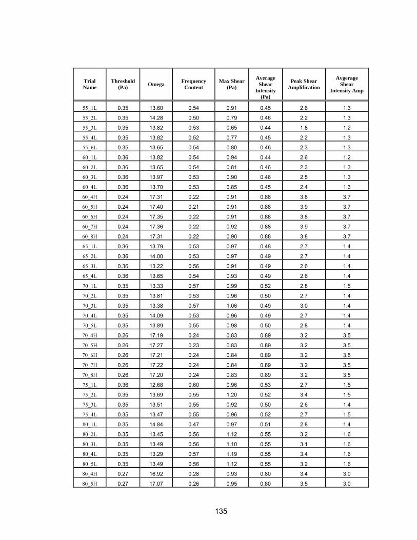
Trial Name

Threshold (Pa) Omega Frequency

Content Max Shear

(Pa)

Average

Shear Intensity

(Pa)

Peak Shear Amplification

Avgerage Shear

Intensity Amp

55_1L 0.35 13.60 0.54 0.91 0.45 2.6 1.3

55_2L 0.35 14.28 0.50 0.79 0.46 2.2 1.3

55_3L 0.35 13.82 0.53 0.65 0.44 1.8 1.2

55_4L 0.35 13.82 0.52 0.77 0.45 2.2 1.3

55_6L 0.35 13.65 0.54 0.80 0.46 2.3 1.3

60_1L 0.36 13.82 0.54 0.94 0.44 2.6 1.2

60_2L 0.36 13.65 0.54 0.81 0.46 2.3 1.3

60_3L 0.36 13.97 0.53 0.90 0.46 2.5 1.3

60_4L 0.36 13.70 0.53 0.85 0.45 2.4 1.3

60_4H 0.24 17.31 0.22 0.91 0.88 3.8 3.7

60_5H 0.24 17.40 0.21 0.91 0.88 3.9 3.7

60_6H 0.24 17.35 0.22 0.91 0.88 3.8 3.7

60_7H 0.24 17.36 0.22 0.92 0.88 3.9 3.7

60_8H 0.24 17.31 0.22 0.90 0.88 3.8 3.7

65_1L 0.36 13.79 0.53 0.97 0.48 2.7 1.4

65_2L 0.36 14.00 0.53 0.97 0.49 2.7 1.4

65_3L 0.36 13.22 0.56 0.91 0.49 2.6 1.4

65_4L 0.36 13.65 0.54 0.93 0.49 2.6 1.4

70_1L 0.35 13.33 0.57 0.99 0.52 2.8 1.5

70_2L 0.35 13.81 0.53 0.96 0.50 2.7 1.4

70_3L 0.35 13.38 0.57 1.06 0.49 3.0 1.4

70_4L 0.35 14.09 0.53 0.96 0.49 2.7 1.4

70_5L 0.35 13.89 0.55 0.98 0.50 2.8 1.4

70_4H 0.26 17.19 0.24 0.83 0.89 3.2 3.5

70_5H 0.26 17.27 0.23 0.83 0.89 3.2 3.5

70_6H 0.26 17.21 0.24 0.84 0.89 3.2 3.5

70_7H 0.26 17.22 0.24 0.84 0.89 3.2 3.5

70_8H 0.26 17.20 0.24 0.83 0.89 3.2 3.5

75_1L 0.36 12.68 0.60 0.96 0.53 2.7 1.5

75_2L 0.35 13.69 0.55 1.20 0.52 3.4 1.5

75_3L 0.35 13.51 0.55 0.92 0.50 2.6 1.4

75_4L 0.35 13.47 0.55 0.96 0.52 2.7 1.5

80_1L 0.35 14.84 0.47 0.97 0.51 2.8 1.4

80_2L 0.35 13.45 0.56 1.12 0.55 3.2 1.6

80_3L 0.35 13.49 0.56 1.10 0.55 3.1 1.6

80_4L 0.35 13.29 0.57 1.19 0.55 3.4 1.6

80_5L 0.35 13.49 0.56 1.12 0.55 3.2 1.6

80_4H 0.27 16.92 0.28 0.93 0.80 3.4 3.0

80_5H 0.27 17.07 0.26 0.95 0.80 3.5 3.0

135

Trial Name

Threshold (Pa) Omega Frequency

Content Max Shear

(Pa)

Average

Shear Intensity

(Pa)

Peak Shear Amplification

Avgerage Shear

Intensity Amp

80_6H 0.27 17.01 0.26 0.95 0.80 3.5 3.0

80_7H 0.27 17.06 0.28 0.95 0.80 3.5 3.0

85_1L 0.34 15.78 0.41 0.84 0.56 2.5 1.7

85_2L 0.34 15.99 0.40 0.95 0.55 2.8 1.6

85_3L 0.34 15.88 0.42 0.86 0.55 2.5 1.6

85_4L 0.34 15.91 0.41 0.86 0.55 2.6 1.6

85_5L 0.34 15.89 0.42 0.88 0.55 2.6 1.6

90_1L 0.32 16.52 0.36 0.98 0.69 3.1 2.2

90_2L 0.29 16.65 0.34 1.00 0.80 3.4 2.7

90_3L 0.33 16.03 0.39 0.93 0.63 2.8 1.9

90_4L 0.31 16.39 0.37 0.97 0.73 3.1 2.3

90_5L 0.33 16.22 0.35 0.87 0.64 2.7 2.0

90_6L 0.32 16.39 0.36 0.93 0.70 2.9 2.2

94_1L 0.30 16.89 0.30 1.04 0.81 3.5 2.7

94_2L 0.31 16.13 0.38 0.93 0.72 3.0 2.3

94_3L 0.30 16.41 0.34 1.11 0.83 3.7 2.8

94_4L 0.30 16.77 0.32 1.05 0.84 3.6 2.8

94_5L 0.29 16.12 0.37 1.12 0.85 3.8 2.9

94_4H 0.27 17.17 0.24 1.07 0.97 4.0 3.6

94_5H 0.27 17.17 0.24 1.07 0.95 4.0 3.6

94_6H 0.27 17.18 0.24 1.06 0.96 4.0 3.6

94_7H 0.27 17.18 0.24 1.07 0.96 4.0 3.6

136

Trial Name

Probability of

Exceedence phi ( ) phi

(tables) time (%)

rate of up-crossings

(samples/s)

time of up-crossings

(s)

mean clump size (samples)

mean duration of

clump (s)

55_1L 11.5 1.20 0.885 11.30 22.61 6.78 23.00 0.12

55_2L 8.1 1.40 0.919 7.71 15.43 4.63 16.00 0.08

55_3L 7.4 1.45 0.926 7.18 14.36 4.31 15.00 0.08

55_4L 9.4 1.32 0.906 7.95 15.89 4.77 16.00 0.08

55_6L 11.1 1.22 0.889 8.85 17.70 5.31 18.00 0.09

60_1L 16.4 0.98 0.836 16.20 32.40 9.72 35.00 0.18

60_2L 16.1 0.99 0.839 15.70 31.40 9.42 35.00 0.18

60_3L 15.4 1.02 0.846 14.49 28.98 8.69 30.00 0.15

60_4L 15.2 1.03 0.848 14.65 29.30 8.79 30.00 0.15

60_4H 99.9 -14.96 0.001 100.00 200.00 60.00 625.00 3.13

60_5H 99.9 -16.58 0.001 100.00 200.00 60.00 650.00 3.25

60_6H 99.9 -15.90 0.001 100.00 200.00 60.00 650.00 3.25

60_7H 99.9 -15.66 0.001 100.00 200.00 60.00 625.00 3.13

60_8H 99.9 -14.83 0.001 100.00 200.00 60.00 625.00 3.13

65_1L 29.5 0.54 0.705 27.64 55.27 16.58 55.00 0.28

65_2L 30.9 0.50 0.691 28.09 56.18 16.85 60.00 0.30

65_3L 28.1 0.58 0.719 26.29 52.59 15.78 55.00 0.28

65_4L 29.1 0.55 0.709 27.23 54.47 16.34 55.00 0.28

70_1L 41.7 0.21 0.583 38.38 76.76 23.03 75.00 0.38

70_2L 41.3 0.22 0.587 37.01 74.02 22.21 75.00 0.38

70_3L 45.3 0.12 0.547 43.13 86.25 25.88 85.00 0.43

70_4L 42.1 0.20 0.579 40.80 81.59 24.48 85.00 0.43

70_5L 42.5 0.19 0.575 41.83 83.67 25.10 85.00 0.43

70_4H 99.9 -13.61 0.001 100.00 200.00 60.00 500.00 2.50

70_5H 99.9 -14.04 0.001 100.00 200.00 60.00 500.00 2.50

70_6H 99.9 -13.83 0.001 100.00 200.00 60.00 500.00 2.50

70_7H 99.9 -13.99 0.001 100.00 200.00 60.00 500.00 2.50

70_8H 99.9 -14.10 0.001 100.00 200.00 60.00 500.00 2.50

75_1L 53.9 -0.10 0.461 54.46 108.91 32.67 110.00 0.55

75_2L 52.4 -0.06 0.476 49.61 99.22 29.77 100.00 0.50

75_3L 53.9 -0.10 0.461 52.66 105.32 31.60 110.00 0.55

75_4L 52.8 -0.07 0.472 51.93 103.86 31.16 110.00 0.55

80_1L 84.4 -1.01 0.156 85.91 171.83 51.55 175.00 0.88

80_2L 68.8 -0.49 0.312 67.09 134.18 40.25 135.00 0.68

80_3L 65.2 -0.39 0.348 67.42 134.84 40.45 135.00 0.68

80_4L 66.3 -0.42 0.337 66.13 132.25 39.68 135.00 0.68

80_5L 69.8 -0.52 0.302 68.02 136.04 40.81 140.00 0.70

80_4H 99.9 -14.01 0.001 100.00 200.00 60.00 450.00 2.25

80_5H 99.9 -13.94 0.001 100.00 200.00 60.00 425.00 2.13

137

Trial Name

Probability of

Exceedence phi ( ) phi

(tables) time (%)

rate of up-crossings

(samples/s)

time of up-crossings

(s)

mean clump size (samples)

mean duration of

clump (s)

80_6H 99.9 -14.00 0.001 100.00 200.00 60.00 450.00 2.25

80_7H 99.9 -13.97 0.001 100.00 200.00 60.00 450.00 2.25

85_1L 99.2 -2.41 0.008 98.86 197.73 59.32 200.00 1.00

85_2L 99.4 -2.52 0.006 99.39 198.78 59.63 195.00 0.98

85_3L 89.9 -2.32 0.101 99.61 199.22 59.77 200.00 1.00

85_4L 91.1 -2.39 0.089 98.90 197.80 59.34 200.00 1.00

85_5L 91.1 -2.39 0.089 99.29 198.58 59.58 200.00 1.00

90_1L 99.9 -5.48 0.001 100.00 200.00 60.00 250.00 1.25

90_2L 99.9 -8.61 0.001 100.00 200.00 60.00 350.00 1.75

90_3L 99.9 -3.81 0.001 100.00 200.00 60.00 225.00 1.13

90_4L 99.9 -6.12 0.001 100.00 200.00 60.00 275.00 1.38

90_5L 99.9 -4.77 0.001 100.00 200.00 60.00 230.00 1.15

90_6L 99.9 -5.55 0.001 100.00 200.00 60.00 275.00 1.38

94_1L 99.9 -10.55 0.001 100.00 200.00 60.00 325.00 1.63

94_2L 99.9 -5.43 0.001 100.00 200.00 60.00 275.00 1.38

94_3L 99.9 -8.76 0.001 100.00 200.00 60.00 325.00 1.63

94_4L 99.9 -9.99 0.001 100.00 200.00 60.00 325.00 1.63

94_5L 99.9 -8.16 0.001 100.00 200.00 60.00 350.00 1.75

94_4H 99.9 -21.18 0.001 100.00 200.00 60.00 425.00 2.13

94_5H 99.9 -20.47 0.001 100.00 200.00 60.00 450.00 2.25

94_6H 99.9 -20.94 0.001 100.00 200.00 60.00 450.00 2.25

94_7H 99.9 -21.28 0.001 100.00 200.00 60.00 425.00 2.13

138

VITAE – Michael W. Horst EDUCATION: Current The Pennsylvania State University - University Park, PA Ph.D. - Civil Engineering (water resources) Focus: Time Variation of Shear Stress Measurements at the Base of Rectangular Piers Advisor: Arthur C. Miller, Ph.D., P.E. May 1999 M.Eng - Civil Engineering (water resources) Advisor: Arthur C. Miller, Ph.D., P.E. May 1996 B.S. – Civil Engineering Minor – Environmental Engineering TEACHING EXPERIENCE: Fall 1999 - The Pennsylvania State University – University Park, PA Current Lecturer: “Applied Hydraulic Engineering” (C.E. 362) Lecturer: “Introduction to Fluid Mechanics” (C.E. 360) Co-Lecturer: “Open Channel Hydraulics” (C.E. 462) Instructor: “Applied Fluid Mechanics Laboratory” (C.E. 363) Co-Instructor: “Engineering Hydrology” (C.E. 361) Teaching Assistant: “Waterways Engineering” (C.E. 465) May 1998 - Continuing Education Courses Current Basic Hydrology, Advanced Hydrology, HEC-1, HEC-HMS, HEC-RAS, Advanced Topics in HEC-RAS, Unsteady Flow Modeling using HEC-RAS PUBLICATIONS: Johnson, P.A., Hey, R.D., Horst, M.W., Hess, A.J., “Aggradation at Bridges,” Journal of Hydraulic Engineering, February 2001, Vol. 127, No. 2, 154-157. Horst, M.W., and Miller, A.C., “Hydrologic Modeling Using GIS

Applications,” Proceeding of the 2001 ASDSO Annual Conference, Snowbird, UT.

Horst, M.W., and Miller, A.C., “Unsteady Flow Routing Utilizing HEC-RAS (3.0),” Proceeding of the 2000 ASDSO Annual Conference, Providence, RI. Horst, M.W., and Miller, A.C., "Uncertainty in the Variables Used to Calculate the PMF for Small Watersheds," Proceedings of the 1999 ASDSO Annual Conference, St. Louis, MO.