Embed Size (px)
Citation preview

Time Series Spectral Representation
0 2 4 6 8 10 12
060
0014
000
Month
Mea
n flo
w m
gal
1 2 3 4 5 6 7 8 9 10 11 12
Alafia River Monthly Mean Streamflow
Z(t) = {Z1, Z2, Z3, … Zn}
)1S()n/kt2Sinbn/kt2Cosa(Z2/n
0kkkt
Any mathematical function has a representation in terms of sin and cos functions.
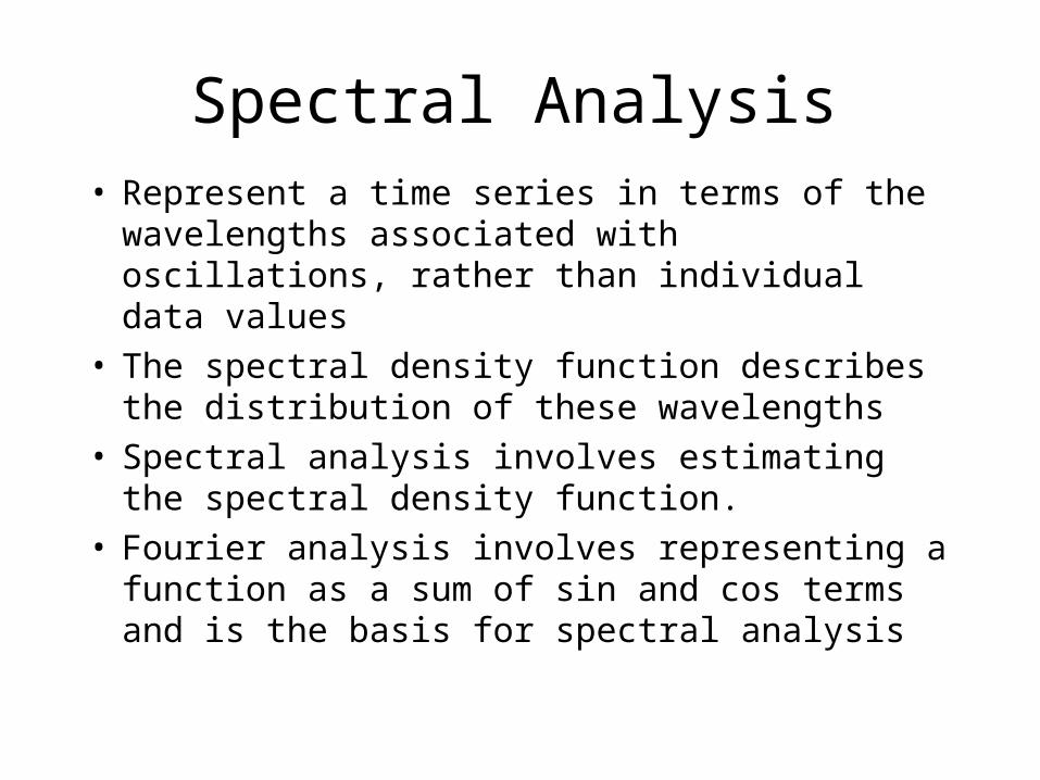
Spectral Analysis• Represent a time series in terms of the
wavelengths associated with oscillations, rather than individual data values
• The spectral density function describes the distribution of these wavelengths
• Spectral analysis involves estimating the spectral density function.
• Fourier analysis involves representing a function as a sum of sin and cos terms and is the basis for spectral analysis

Why Spectral Analysis
• Yields insight regarding hidden periodicities and time scales involved
• Provides the capability for more general simulation via sampling from the spectrum
• Supports analytic representation of linear system response through its connection to the convolution integral
• Is widely used in many fields of data analysis

Frequency and Wavenumber
)2S()tSinwbtCoswa(Z2/n
0kkkkkt
n/k2wk n/kfk
Due to orthogonality of Sin and Cos functions
)3S(
2
1n...1ktCoswZ
n
2
evennif2/n,0ktCoswZn
1
an
1tkt
n
1tkt
k
)4S(tSinwZn
2b
n
1tktk
cycles/time radians/time

Frequency Limits
Lowest frequency resolved
Highest frequency resolved, corresponds to n/2 (Nyquist frequency)
General case, time interval ∆t
Nw 2/1fN
n/2w1 n/1f1
t/wN t2/1fN
tn/2w1 tn/1f1
1
k
kw
tn/k2w

AliasingDue to discretization, a sparsely sampled high frequency process may be erroneously attributed to a lower frequency
0 1 2 3 4 5 6
-1.0
-0.5
0.0
0.5
1.0
t

Example. Fourier representation of streamflow
1 2 3 4 5 650
015
0025
0035
00
k
sqrt
(a *
a +
b *
b)
0 2 4 6 8 10 12
040
0010
000
Month
Mea
n flo
w m
gal
1 3 5 7 9 11
Alafia River Monthly Mean Streamflow

Equivalent complex number representation
wsiniwcoseiw
)6S(eZn
1C
n
1t
tiwtk
k
)5S(eCZ)2/n(trunc
21n
trunck
tiwkt
k
Note: Integer truncation is used in the sum limits. For example if n=5 (odd) the limits are -2, 2. If n=6 (even) the limits are -2, 3. (Same number of fourier coefficients as data points)
n/k2wk
Complex conjugate pair
kk wn/k2w
*kk CC
2
ibaC kk
k
2
ibaC kk*
k

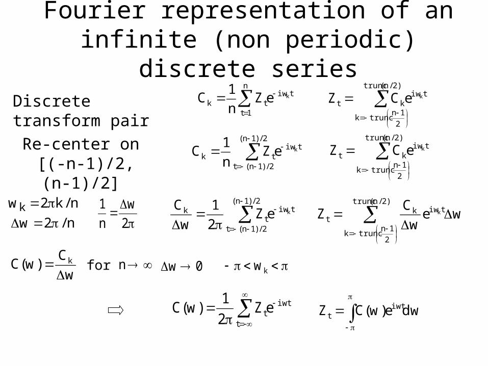
Fourier representation of an infinite (non periodic) discrete series
n
1t
tiwtk
keZn
1C
)2/n(trunc
2
1ntrunck
tiwkt
keCZDiscrete transform pair
n/2w1
n/2w
Lowest frequency
Highest frequency
Spacing
As
Nw
n 0w
w- on continuous wwkwk
0.0 0.5 1.0 1.5 2.0 2.5 3.0
0.2
0.8
wk
Ck
w
0.0 0.5 1.0 1.5 2.0 2.5 3.0
0.2
0.8
wk
Ck
0.0 0.5 1.0 1.5 2.0 2.5 3.00.
20.
8
wk
Ck
Fourier representation of an infinite (non periodic) discrete series
n
1t
tiwtk
keZn
1C
)2/n(trunc
2
1ntrunck
tiwkt
keCZ
n/k2wk n/2w
Discrete transform pair
2/)1n(
2/)1n(t
tiwtk
keZn
1C
)2/n(trunc
2
1ntrunck
tiwkt
keCZRe-center on [(-n-1)/2, (n-1)/2]
2
w
n
1
n
2/)1n(
2/)1n(t
tiwt
k keZ2
1
w
Cwe
w
CZ
)2/n(trunc
2
1ntrunck
tiwkt
k
w
C)w(C k
for 0w
t
iwtteZ
2
1)w(C
kw
dwe)w(CZ iwtt
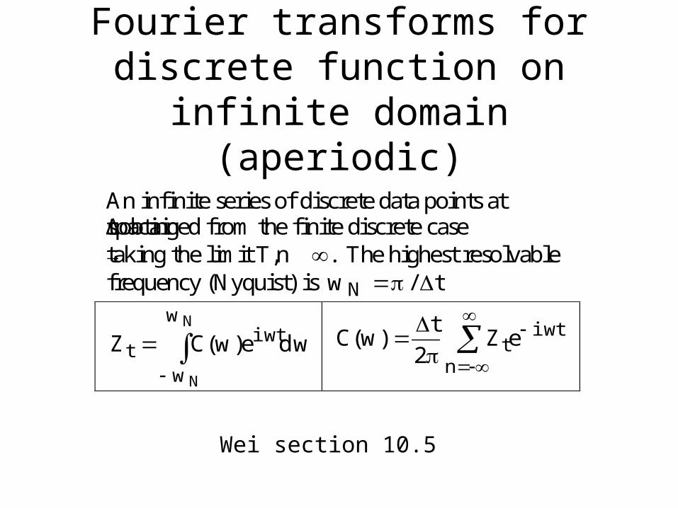
Fourier transforms for discrete function on infinite domain
(aperiodic)
An infinite series of discrete data points at spacing ∆t obtained from the finite discrete case taking the limit T,n→ . The highest resolvable frequency (Nyquist) is t/w N
dwe)w(CZN
N
w
w
iwtt
n
iwtteZ
2
t)w(C
Wei section 10.5
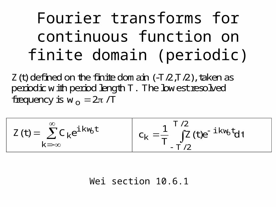
Fourier transforms for continuous function on finite domain (periodic)
Z(t) defined on the finite domain (-T/2,T/2), taken as periodic with period length T. The lowest resolved frequency is T/2wo
k
tikwk
oeC)t(Z dte)t(ZT
1c
2/T
2/T
tikwk
o
Wei section 10.6.1

Fourier transforms for continuous function on infinite domain
(aperiodic)
Z(t) defined on the entire interval (-,), obtained from the finite domain case by letting T→ . All frequencies are resolved.
w
iwtdwe)w(C)t(Z
t
iwtdte)t(Z2
1)w(C
The placement of 2π in this definition varies amongst references
Wei section 10.6.2

Frequency domain representation of a random process
• Z(t) and C(w) are alternative equivalent representations of the data
• If Z(t) is a random process C(w) is also random
• ACF(Z(t))≡Spectral density function(C(w))

1940 1950 1960 1970 1980 1990 2000
020
000
6000
0
Year
mga
l
Alafia River Streamflow
Spectral decomposition of any function
n
1t
tiwtk
keZn
1c
0 100 200 300 400
050
010
00
k
ck
1.04 2.087 3.134

0 10 20 30 40 50 60
-10
12
1:n1
z[1:
n1]
0 5 10 15 20
0.0
0.4
0.8
Lag
AC
F
Series z
0.0 0.1 0.2 0.3 0.4 0.5
02
46
810
Frequency
Pow
er
0.0 0.1 0.2 0.3 0.4 0.5
0.5
1.0
2.0
frequency
spec
trum
Series: zSmoothed Periodogram
bandwidth = 0.0197
Spectral representation of a stationary random process
Time Series
Smoothing
Fourier Transform
Autocorrelation
Fourier Transform
Fourier coefficients Spectral density function
Autocorrelation function

Time Domain Frequency Domain
)t(Z )w(C
Z1, Z2, Z3, … C1, C2, C3, …
0 5 10 15 20
0.0
0.4
0.8
Lag
AC
F
Series z
0.0 0.1 0.2 0.3 0.4 0.5
01
23
45
67
Frequency
Pow
er

0.0 0.1 0.2 0.3 0.4 0.5
01
23
45
67
Frequency
Pow
er
The Periodogram|Ck|2 is random because Zt is random
Power at low frequency Persistence indicated by ACF
2k
2t |C|Z
n
1
Decomposition of variance
|Ck|2
k/n
Wei section 12.1
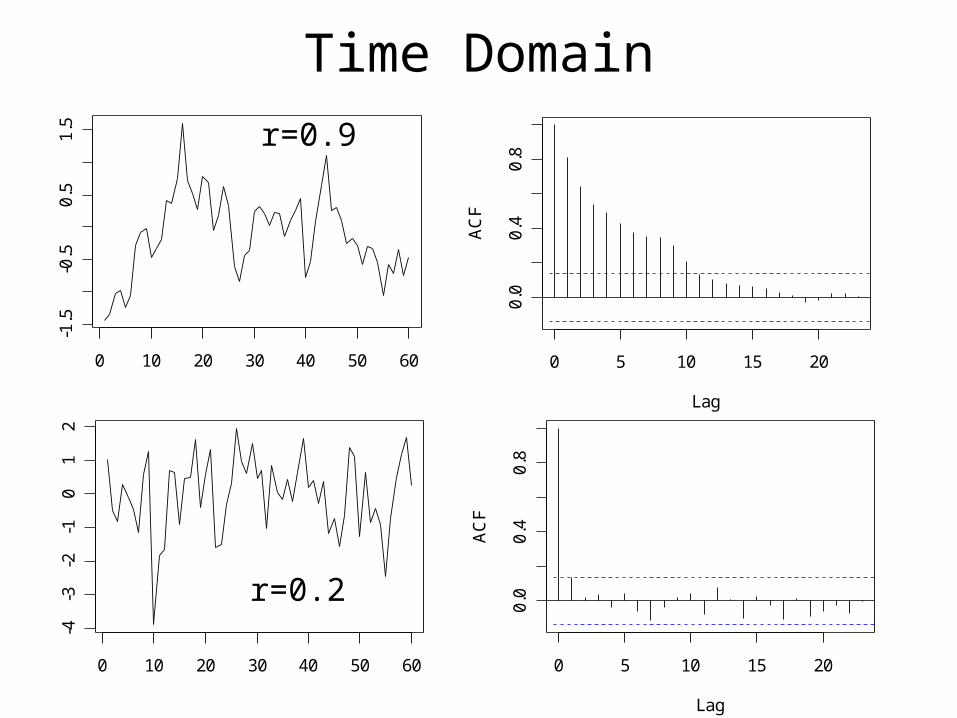
0 10 20 30 40 50 60
-1.5
-0.5
0.5
1.5
1:n1
z[1:
n1]
0 5 10 15 20
0.0
0.4
0.8
Lag
AC
F
Series z
0 5 10 15 20
0.0
0.4
0.8
Lag
AC
F
Series z
0 10 20 30 40 50 60
-4-3
-2-1
01
2
1:n1
z[1:
n1]
r=0.9
r=0.2
Time Domain

0 10 20 30 40 50 60
-1.5
-0.5
0.5
1.5
1:n1
z[1:
n1]
0 10 20 30 40 50 60
-4-3
-2-1
01
2
1:n1
z[1:
n1]
r=0.9
r=0.2
Frequency Domain
0.0 0.1 0.2 0.3 0.4 0.5
01
23
4
Frequency
Pow
er
0.0 0.1 0.2 0.3 0.4 0.5
02
46
810
Frequency
Pow
er
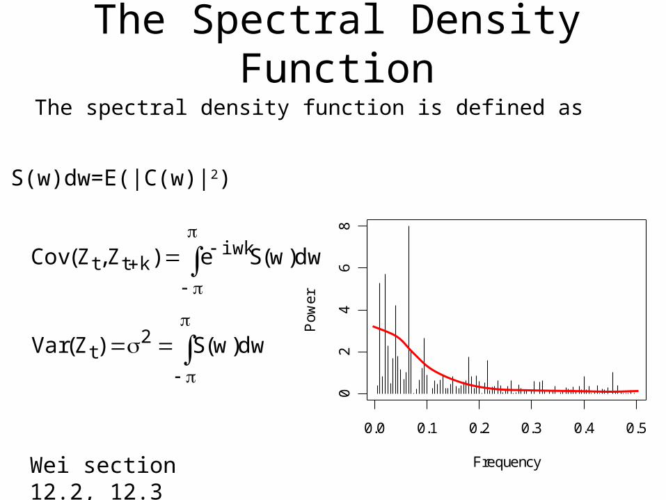
The Spectral Density Function
The spectral density function is defined as
0.0 0.1 0.2 0.3 0.4 0.5
02
46
8
Frequency
Pow
er
dw)w(Se)Z,Z(Cov iwk
ktt
S(w)dw=E(|C(w)|2)
dw)w(S)Z(Var 2t
Wei section 12.2, 12.3

Problem Estimating S(w)
• Z(t) Stationary C(w) Independent
• |C(w)|2 has 2 degrees of freedom (from real and imaginary parts
• More data ∆w gets smaller, but still 2 degrees of freedom
0.0 0.1 0.2 0.3 0.4 0.5
02
46
8
Frequency
Pow
er
0.1 0.2 0.3 0.4 0.5
02
46
8
Frequency
Pow
er
n=50 n=200

S(w) estimated by smoothing the periodogram
• Balance Spectral resolution versus precision• Tapering to minimize leakage to adjacent
frequencies • Confidence bounds by 2 based on number of
degrees of freedom involved with smoothing• Multitaper methods• A lot of lore

0.0 0.1 0.2 0.3 0.4 0.5
05
1015
Frequency
Pow
er
Different degrees of smoothing
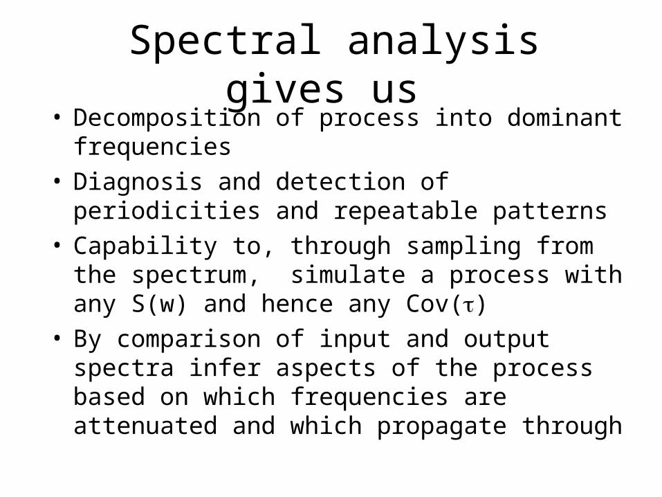
Spectral analysis gives us • Decomposition of process into dominant frequencies• Diagnosis and detection of periodicities and
repeatable patterns• Capability to, through sampling from the spectrum,
simulate a process with any S(w) and hence any Cov()
• By comparison of input and output spectra infer aspects of the process based on which frequencies are attenuated and which propagate through


![arXiv:1305.7375v2 [physics.comp-ph] 5 Jun 2013 · k0v t 2 cos k0 yv 2 cos k0 z v z t 2 1 3 sin k0 y v 2 sin k0 z v 2 =k sin k0 yv t cos k0 zv z t 2 cos k 0 xv x t 2 1 3 sin k 0 z](https://img.pdfslide.us/doc/110x75/5e6d6755adc6cb7d4075a992/arxiv13057375v2-5-jun-2013-k0v-t-2-cos-k0-yv-2-cos-k0-z-v-z-t-2-1-3-sin-k0.jpg)