Time Series Project Report

Data Set Analysis Report

Xiao Ma

Nov 16th, 2016

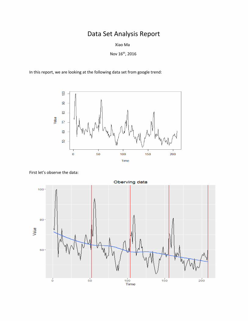
In this report, we are looking at the following data set from google trend:

First let’s observe the data:

From the plot above, it is obvious that the data set has a very clear trend of decreasing, which is possibly

linear. Also, the vertical lines dividing the total 208 observations into 4 sections also reveal that there is

a seasonality in the data set with period around 52.

1. Fitting the model with the method of differencing

As we know, a time series X(t)=m(t)+s(t)+Z(t) where m(t) is the trend, s(t) is the seasonality and Z(t)

denotes the white noise.

Since based on the observation, I'm confident that there is a trend as well as a seasonality within the

data and I will eventually fit a seasonal ARIMA model, it is reasonable to consider this time series as:

X(t)=m(t)+Z1(t)+s(t)+Z2(t) where Z1(t) is the white noise affecting the trend function and Z2(t) is the white

noise affecting the seasonal function. By studying Z1 and Z2 separately, I believe that I'll be able to find

more accurate values for p,d,q and P,D,Q.

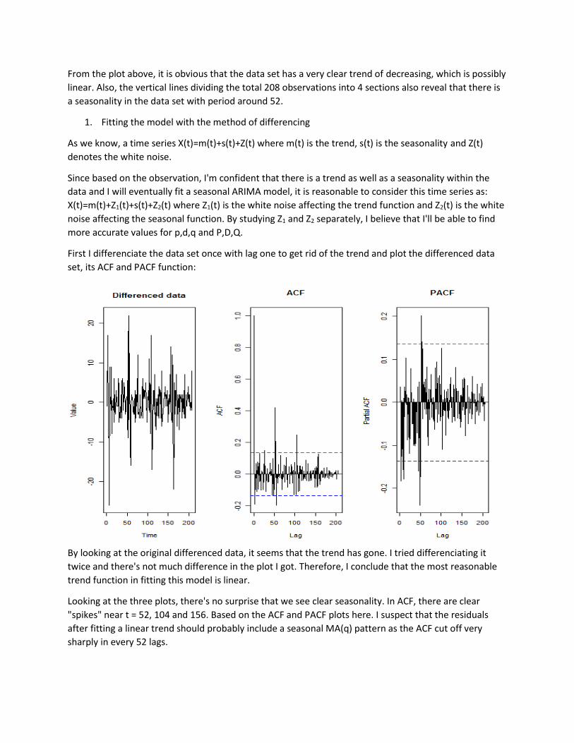
First I differenciate the data set once with lag one to get rid of the trend and plot the differenced data

set, its ACF and PACF function:

By looking at the original differenced data, it seems that the trend has gone. I tried differenciating it

twice and there's not much difference in the plot I got. Therefore, I conclude that the most reasonable

trend function in fitting this model is linear.

Looking at the three plots, there's no surprise that we see clear seasonality. In ACF, there are clear

"spikes" near t = 52, 104 and 156. Based on the ACF and PACF plots here. I suspect that the residuals

after fitting a linear trend should probably include a seasonal MA(q) pattern as the ACF cut off very

sharply in every 52 lags.

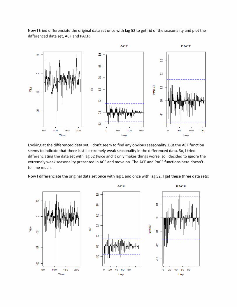
Now I tried differenciate the original data set once with lag 52 to get rid of the seasonality and plot the

differenced data set, ACF and PACF:

Looking at the differenced data set, I don't seem to find any obvious seasonality. But the ACF function

seems to indicate that there is still extremely weak seasonality in the differenced data. So, I tried

differenciating the data set with lag 52 twice and it only makes things worse, so I decided to ignore the

extremely weak seasonality presented in ACF and move on. The ACF and PACF functions here doesn't

tell me much.

Now I differenciate the original data set once with lag 1 and once with lag 52. I get these three data sets:

Here the ACF cuts off at lag 1 and PACF tails off (although in a wired way), So it will be reasonable to fit a

MA(1) for the non-seasonal part of our model. Together with the previous two ACF and PACF plots, I

think that ARIMA(0,1,1)X(0,1,1)_52 should be a good fit. I tuned the parameters and get the first four

ARIMA models. There are other possible ways of tuning parameters. Being not sure about the messy

ACF and PACF, I also want to test out some models that looks not very reasonable or farfetched like the

fifth and the sixth model:

DS1arima1=ARIMA(0,1,1)X(0,1,1)52

DS1arima2= ARIMA(0,1,1)X(0,1,2)52

DS1arima3= ARIMA(0,1,2)X(0,1,2)52

DS1arima4= ARIMA(0,1,2)X(0,1,1)52

DS1arima5= ARIMA(0,1,3)X(0,1,3)52

DS1arima6= ARIMA(0,2,2)X(0,1,2)52

2. Parametric Fitting

After doing differeciation, I also did parametric fitting.

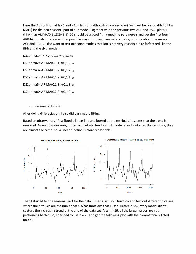
Based on observation, I first fitted a linear line and looked at the residuals. It seems that the trend is

removed. Again, to make sure, I fitted a quadratic function with order 2 and looked at the residuals, they

are almost the same. So, a linear function is more reasonable.

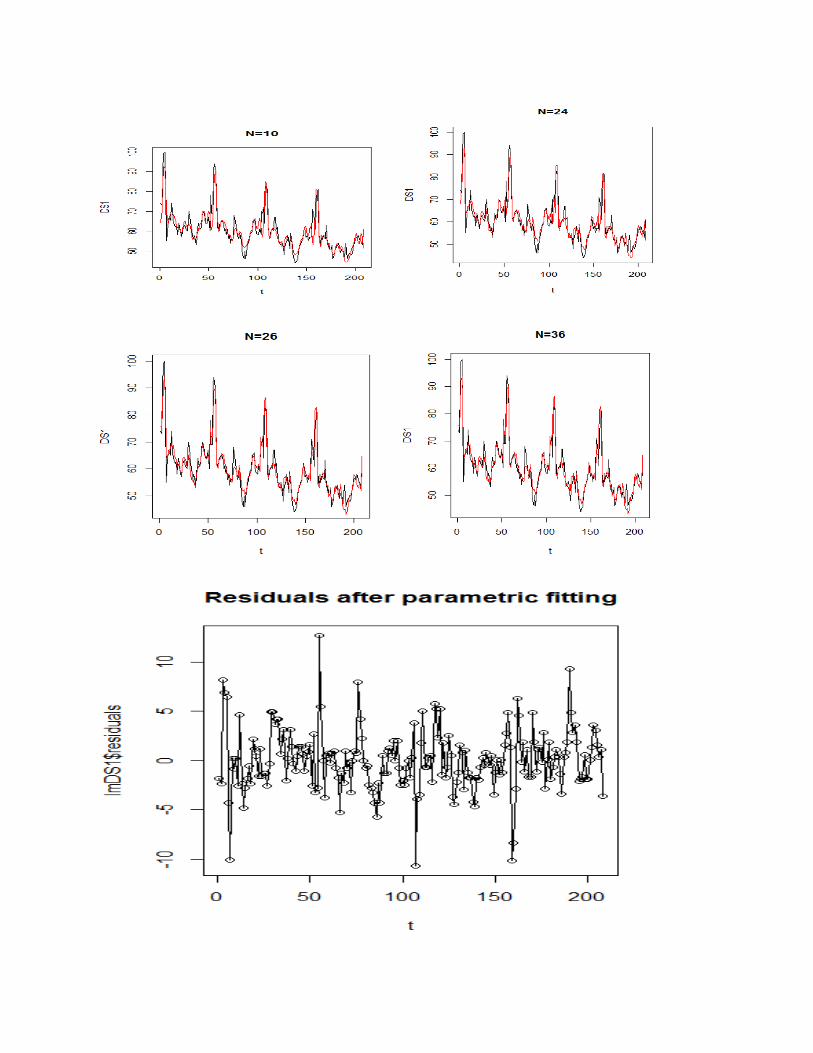
Then I started to fit a seasonal part for the data. I used a sinusoid function and test out different n values

where the n values are the number of sin/cos functions that I used. Before n=26, every model didn’t

capture the increasing trend at the end of the data set. After n=26, all the larger values are not

performing better. So, I decided to use n = 26 and get the following plot with the parametrically fitted

model:

3. Testing Models

Now I look at the AICs and BICs:

AIC BIC AIC preferred? BIC preferred?

Arima1 903.1713 912.3016 No No

Arima2 903.3360 915.5097 No No

Arima3 886.2708 901.4879 No No

Arima4 885.5907 897.7644 Yes Yes

Arima5 890.0773 911.3813 No No

Arima6 913.3885 928.5733 No No

Parametric 1253.9157 1340.6916 No No

It seems that the DS1arima4 is preferred by AIC and BIC.

Then I try CV:

Arima1 Arima2 Arima3 Arima4 Arima5 Arima6

1 12.97968 12.94987 12.27623 12.33738 17.42759 11.68957

2 25.35787 25.35787 39.89730 33.85767 24.82705 28.56950

From the MSEs calculated above, it seems that Arima2 and Arima1 are performing better and more

consistent in the CV testing. Arima3, while preferred by both AIC and BIC, seems to do worse in

predicting. Surprisingly, Arima6 has a decently low value. But due to its bigger number of parameters, I

would choose Arima1 or Arima2 over it.

It is a hard choice choosing between Arima1 and Arima2. They have the same second value and even

though Arima2's first MSE is lower, I eventually decided to go with Arima1 because it's simpler and has

lower AIC as well as BIC comparing with Arima2.

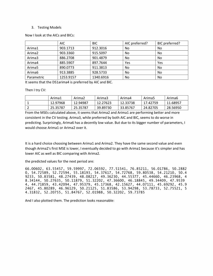
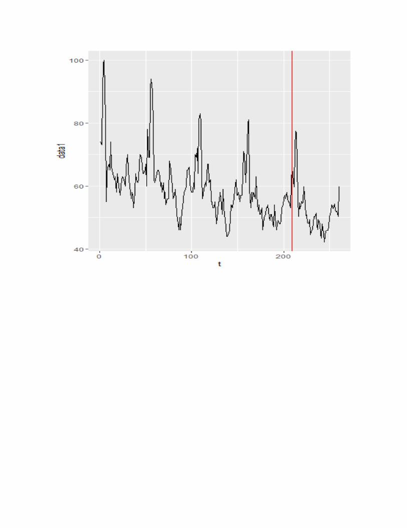
the predicted values for the next period are:

66.00602, 63.55457, 59.59997, 72.06592, 77.51541, 76.85211, 56.01786, 50.28820, 54.72589, 52.72594, 55.18193, 54.37617, 54.72768, 59.80538, 54.21210, 50.49233, 50.83581, 48.27439, 48.08217, 49.36230, 44.55377, 45.44660, 46.23968, 48.34144, 50.27635, 50.11879, 51.32202, 47.36600, 46.18845, 49.34409, 47.95394, 44.71859, 43.42094, 47.95379, 45.17368, 42.15627, 44.07111, 45.69292, 45.92467, 45.80289, 46.96129, 50.21125, 51.83586, 53.94298, 53.78733, 52.75521, 54.31832, 52.20755, 51.84767, 52.01988, 50.32202, 59.73785

And I also plotted them. The prediction looks reasonable:

Appendix (R code)

library(dplyr)

library(ggplot2)

library(printr)

DS1<-read.csv("C:/Users/marsh/Desktop/STAT/STAT153/Project/1DS.csv")

DS1<-ts(DS1)

colnames(DS1)=c("Value")

plot(DS1)

###Differencing

DifDS_noTrend=diff(DS1,differences = 1)

plot(DifDS_noTrend)

acf(DifDS_noTrend,lag.max = 110)

pacf(DifDS_noTrend, lag.max = 110)

DifDS_noSeason=diff(DS1,differences = 1,lag = 52)

plot(DifDS_noSeason)

acf(DifDS_noSeason)

pacf(DifDS_noSeason)

acf(DifDS_noSeason,lag.max = 200)

pacf(DifDS_noSeason,lag.max = 200)

DifDs<-diff(diff(DS1,differences = 1,lag = 52),differences = 1)

plot(DifDs)

acf(DifDs,lag.max = 100)

pacf(DifDs,lag.max = 200)

acf(DifDs,lag.max = 200)

#looks like we have a MA(2) with a seasonal period 52

t<-1:208

DS1arima1=arima(DS1,order = c(0,1,2),seasonal = list(order=c(0,1,2),period=52))

DS1arima1a=arima(DS1,order = c(0,1,1),seasonal = list(order=c(0,1,2),period=52))

DS1arima1b=arima(DS1,order = c(0,1,2),seasonal = list(order=c(0,1,1),period=52))




#personally I prefer the first model

#Parametric fitting

plot(DS1)

t<-1:208

lmDS1<-lm(DS1~t+I(t^2))

plot(lmDS1$residuals,type = 'l', main="residuals after fitting a quadratic")

d<-52

sinusoid <- function(k){

df <- matrix(NA, length(t), 2*k)

for(i in 1:k){

df[, 2 * i - 1] <- cos(2*pi*i*t/d)

df[, 2 * i] <- sin(2*pi*i*t/d)

}

return(as.data.frame(df))

}

lmDS1<-lm(DS1~.,t+sinusoid(k=24))

plot(t,lmDS1$residuals,type = "o",main = "Residuals after parametric fitting")

plot(t, DS1, type = "l",main = "N=24")

points(t, lmDS1$fitted.values, type = "l", col = "red")

################AIC################

AIC(DS1arima1)

AIC(DS1arima1a)

AIC(DS1arima1b)#favored

AIC(DS1arima2)

AIC(DS1arima3)

AIC(DS1arima4)

AIC(lmDS1)

##############BIC################

BIC(DS1arima1)

BIC(DS1arima1a)

BIC(DS1arima1b)#favored

BIC(DS1arima2)

BIC(DS1arima3)

BIC(DS1arima4)

BIC(lmDS1)

####################CV###################

computeCVmse <- function(order.totry, seasorder.totry,data){

MSE <- numeric()

len=length(DS1)

for(k in 1:2){

train.dt <-DS1[1:(len - 52 * k)]

test.dt <- DS1[(len - 52 * k + 1):(len - 52 * (k - 1))]

mod <- arima(train.dt, order = order.totry, seasonal =

list(order = seasorder.totry, period = 52))

fcast <- predict(mod, n.ahead = 52)

MSE[k] <- mean((fcast$pred - test.dt)^2)

}

return(MSE)

}

MSE1<-computeCVmse(c(0,1,2),c(0,1,2),DS1)

MSE1a<-computeCVmse(c(0,1,1),c(0,1,2),DS1)

MSE1b<-computeCVmse(c(0,1,2),c(0,1,1),DS1)




MSE1

MSE1a#favored

MSE1b

MSE2

MSE3#favored

MSE4

##########################################################################

pred1<-predict(DS1arima1a,52)

t<-1:260

data1<-c(DS1,pred1$pred)

pred1DF<-data.frame(x=t,y=data1)

ggplot(pred1DF,aes(x=t,y=data1))+geom_line()+geom_vline(xintercept = 209,col='red')

pred1$pred

Documents

Time Series Project Report