STAT758Final Project

Time series analysis of daily exchange rate between the British Pound and the

US dollar (GBP/USD)

Theophilus Djanie and Harry Dick ThompsonUNR • May 14, 2012

INTRODUCTION

Time Series Analysis accounts for the fact that data points taken over time may have an

internal structure (such as autocorrelation, trend or seasonal variation) that should be

accounted for. The behavior of time series variables such as exchange rates is not

consistent and to forecast it is irrational. Despite these assertions, many multinational

corporations, dealers in foreign exchange, exporters, importers and speculators continue

to make hedging decisions based on forecasted rates using ex-post data as their basis.

These hedging decisions are made under the premise that patterns exist in the ex-post

data and these patterns provide an indication of future movement of exchange rates, at

least in the short run. If such patterns exist, then it is possible in principle to apply

modern mathematical tools and techniques such as ARIMA and GARCH to forecast the

ex-ante exchange rates (Hamilton 1994, Klaassen 1998).

The ARMA model is made up of two processes: the Autoregressive AR and the Moving

Average MA. Given a series Xt, we can model the level of its current observations

depends on the level of its lagged observations. This way of thinking can be represented

by the AR model.

Also we can model that the observations of a random variable at time t are not only

affected by the shock at time t, but also the shocks that have taken place before time t.

This way of thinking can be represented by the MA model.

AutoRegressive Integrated Moving Average (ARIMA) models intend to describe the current

behavior of variables in terms of linear relationships with their past values. It has an

Integrated (I) component (d), which represents the amount of differencing to be performed

on the series to make it stationary. The second component of the ARIMA consists of an

ARMA model for the series rendered stationary through differentiation. The ARMA

component is further decomposed into AR and MA components which are explained

above. The Autocorrelation Function (ACF) and Partial Autocorrelation Function (PACF) are

used to estimate the values of the orders of the AR and MA processes respectively. The

statistical package R is used to analyze the data.

OBJECTIVE

The goal of this study is to perform statistical analysis on the foreign exchange data

between the GBP (Great Britain Pound) and the USD (United States dollar). The properties

of the data are described and basic time series techniques are applied to the data. Plots

of the series, autocorrelation function and the partial autocorrelation function are some

of the graphical tools used to analyze the series. We also aim to fit a model (ARMA,

ARCH, and GARCH) to the data in order to make credible forecasts from the model.

The data used for analysis is the close of business (COB) day value of the daily

exchange rate between the British Pound and the US dollar (GBP/USD). The data was

downloaded from the Oanda Corporation financial services website (http://

www.oanda.com/currency/historical-rates/), from 1st January, 2000 to 4th April, 2012.

Values on weekday holidays are assumed to be the value from the previous business

day. For any other unexpected closure of the market of a single weekday, or several

consecutive weekdays, the data points are filled in with the last COB value. A year of

data is considered to be 52 weeks with five business days per week which equals 366

data points per year.

EXPLORATIVE DATA ANALYSIS AND DESCRIPTIVE OF STATISTICS

The data set is made up of 4478 daily quotes of foreign exchange rate between the GBP

and the USD for the period year 2000 to 2012. The time series analysis for the

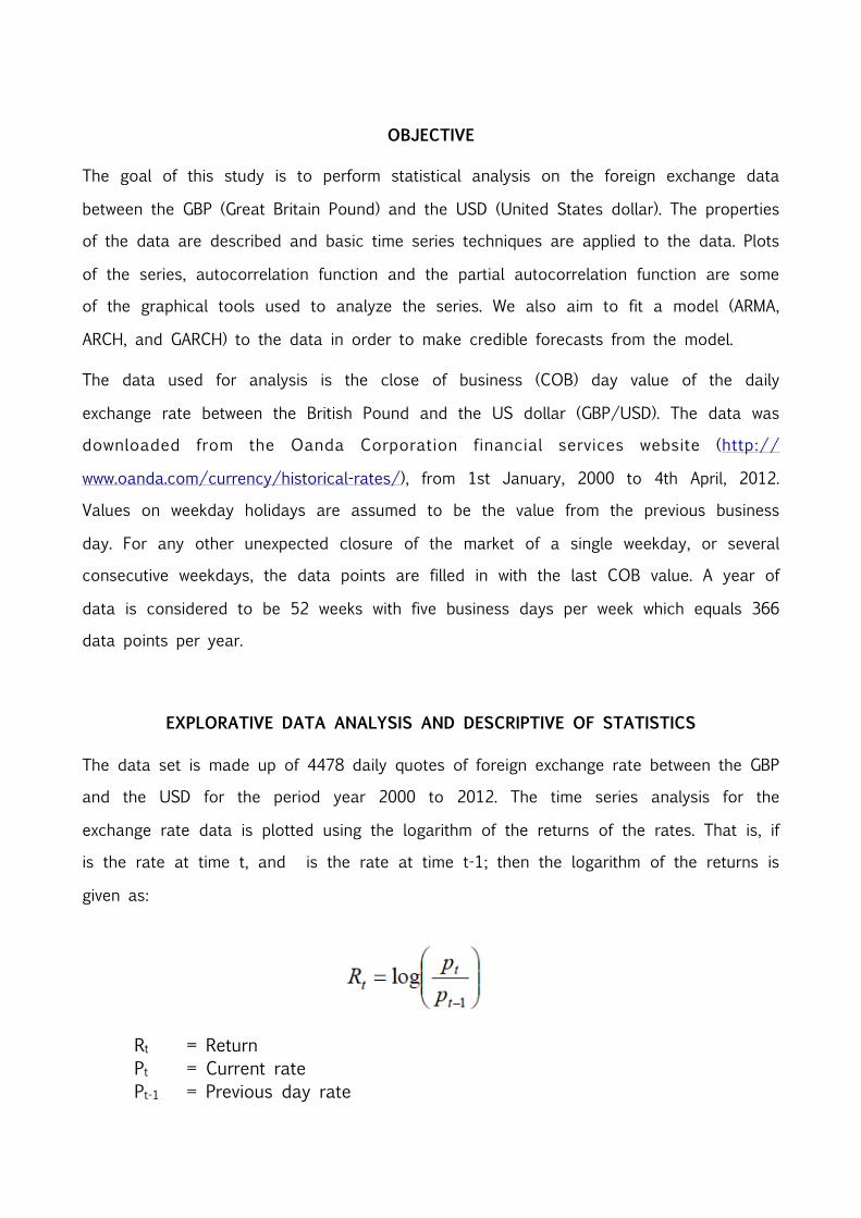
exchange rate data is plotted using the logarithm of the returns of the rates. That is, if

is the rate at time t, and is the rate at time t-1; then the logarithm of the returns is

given as:

Rt = Return Pt = Current rate Pt-1 = Previous day rate

This is because, the log returns of exchange rates have interesting statistical properties;

thus making analysis easier. Also, the log returns are assumed to be normally distributed,

which simplifies computations on the probabilistic aspect of the data. A histogram

illustrating this assumption is shown in fig a below. Some basic (descriptive) statistics of

this data set is given fig1. below.

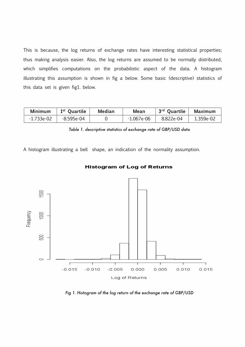
Minimum 1st Quartile Median Mean 3rd Quartile Maximum-1.733e-02 -8.595e-04 0 -1.067e-06 8.822e-04 1.359e-02

Table 1. descriptive statistics of exchange rate of GBP/USD data

A histogram illustrating a bell shape, an indication of the normality assumption.

Fig 1. Histogram of the log return of the exchange rate of GBP/USD

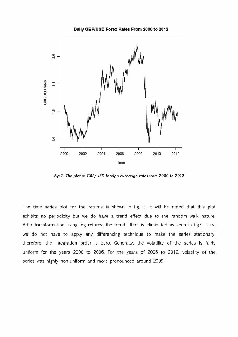
Fig 2. The plot of GBP/USD foreign exchange rates from 2000 to 2012

The time series plot for the returns is shown in fig. 2. It will be noted that this plot

exhibits no periodicity but we do have a trend effect due to the random walk nature.

After transformation using log returns, the trend effect is eliminated as seen in fig3. Thus,

we do not have to apply any differencing technique to make the series stationary;

therefore, the integration order is zero. Generally, the volatility of the series is fairly

uniform for the years 2000 to 2006. For the years of 2006 to 2012, volatility of the

series was highly non-uniform and more pronounced around 2009.

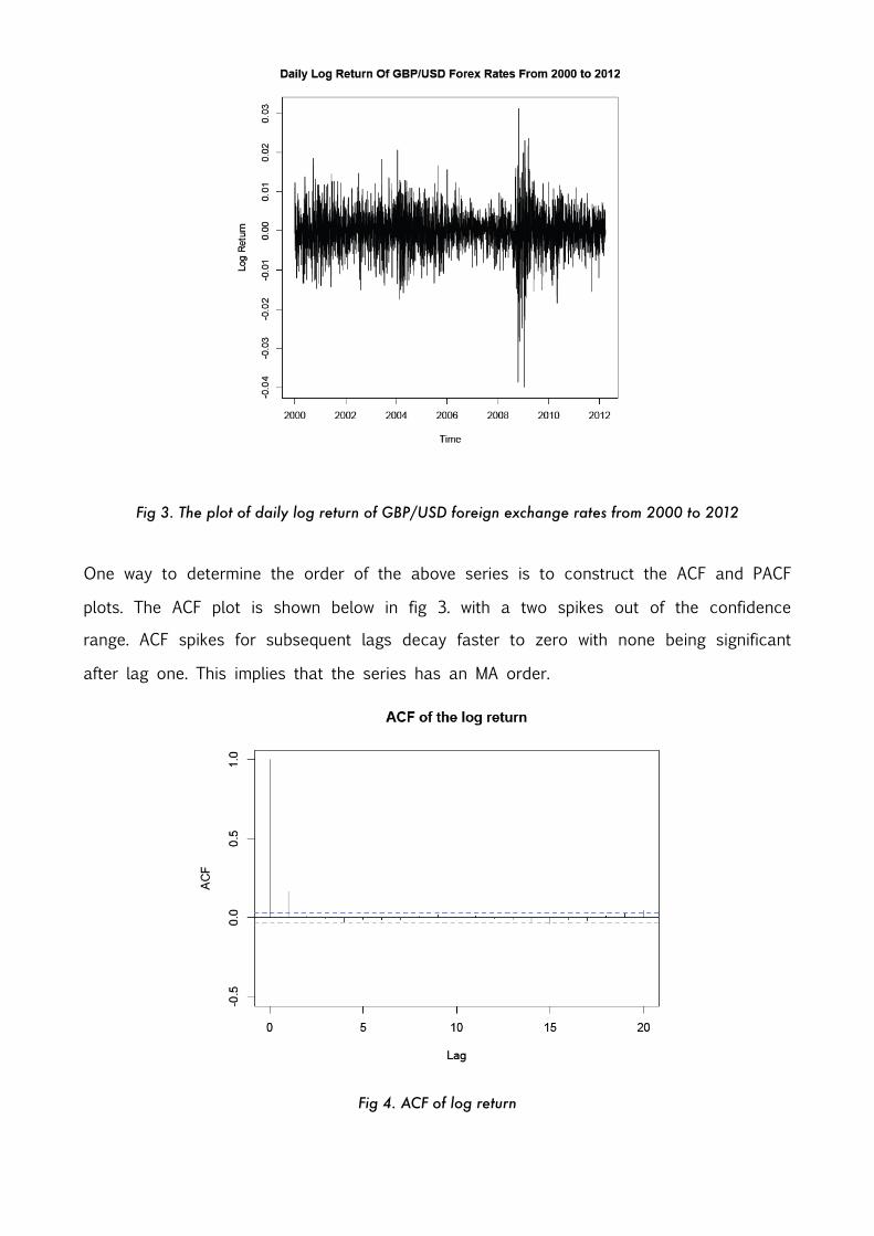
Fig 3. The plot of daily log return of GBP/USD foreign exchange rates from 2000 to 2012

One way to determine the order of the above series is to construct the ACF and PACF

plots. The ACF plot is shown below in fig 3. with a two spikes out of the confidence

range. ACF spikes for subsequent lags decay faster to zero with none being significant

after lag one. This implies that the series has an MA order.

Fig 4. ACF of log return

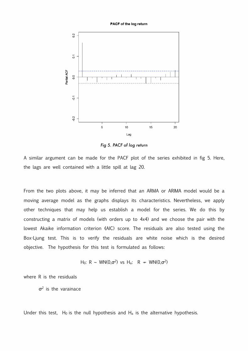
Fig 5. PACF of log return

A similar argument can be made for the PACF plot of the series exhibited in fig 5. Here,

the lags are well contained with a little spill at lag 20.

From the two plots above, it may be inferred that an ARMA or ARIMA model would be a

moving average model as the graphs displays its characteristics. Nevertheless, we apply

other techniques that may help us establish a model for the series. We do this by

constructing a matrix of models (with orders up to 4x4) and we choose the pair with the

lowest Akaike information criterion (AIC) score. The residuals are also tested using the

Box-Ljung test. This is to verify the residuals are white noise which is the desired

objective. The hypothesis for this test is formulated as follows:

H0: R ~ WN(0,σ2) vs Ha: R ≁ WN(0,σ2)

where R is the residuals

σ2 is the varainace

Under this test, H0 is the null hypothesis and Ha is the alternative hypothesis.

ARIMA ANALYSIS

Tables 1-3 in the appendix shows the output of ARIMA models with orders p and q

values ranging from zero to four. In table 1 we realize that the minimum AIC value is

-3.5779.39 and belongs to the model ARIMA (0, 0, 1). The standard error at the specified

p and q values also exhibits a minimum gradient to higher order. The box test for this

model passed the random test.

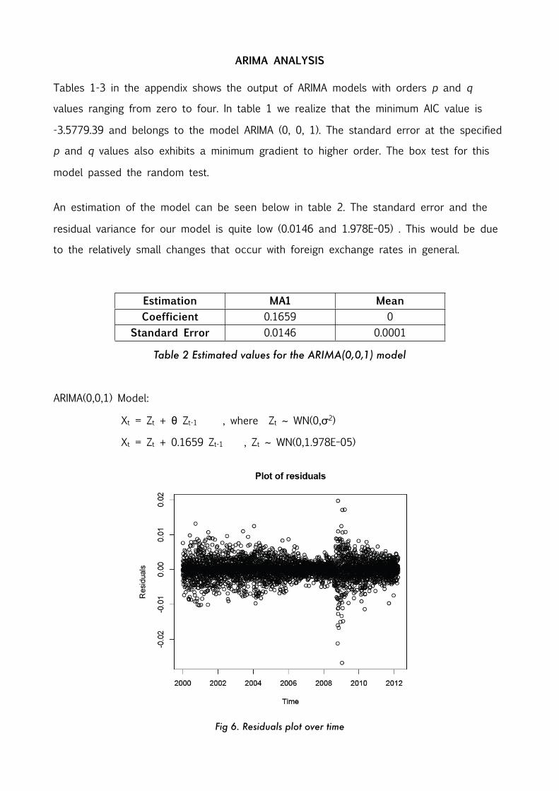
An estimation of the model can be seen below in table 2. The standard error and the

residual variance for our model is quite low (0.0146 and 1.978E−05) . This would be due

to the relatively small changes that occur with foreign exchange rates in general.

Estimation MA1 MeanCoefficient 0.1659 0

Standard Error 0.0146 0.0001

Table 2 Estimated values for the ARIMA(0,0,1) model

ARIMA(0,0,1) Model:

Xt = Zt + θ Zt-1 , where Zt ~ WN(0,σ2)

Xt = Zt + 0.1659 Zt-1    , Zt ~ WN(0,1.978E−05)

Fig 6. Residuals plot over time

The residual of this model is shown below in fig.6. It can be observed that residuals have

a value of zero but displays a non-constant spread especially during 2006 to 2012.

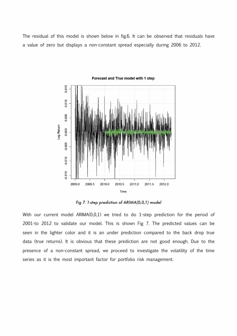
Fig 7. 1-step prediction of ARIMA(0,0,1) model

With our current model ARIMA(0,0,1) we tried to do 1-step prediction for the period of

2001-to 2012 to validate our model. This is shown Fig 7. The predicted values can be

seen in the lighter color and it is an under prediction compared to the back drop true

data (true returns). It is obvious that these prediction are not good enough. Due to the

presence of a non-constant spread, we proceed to investigate the volatility of the time

series as it is the most important factor for portfolio risk management.

GARCH ANALYSIS

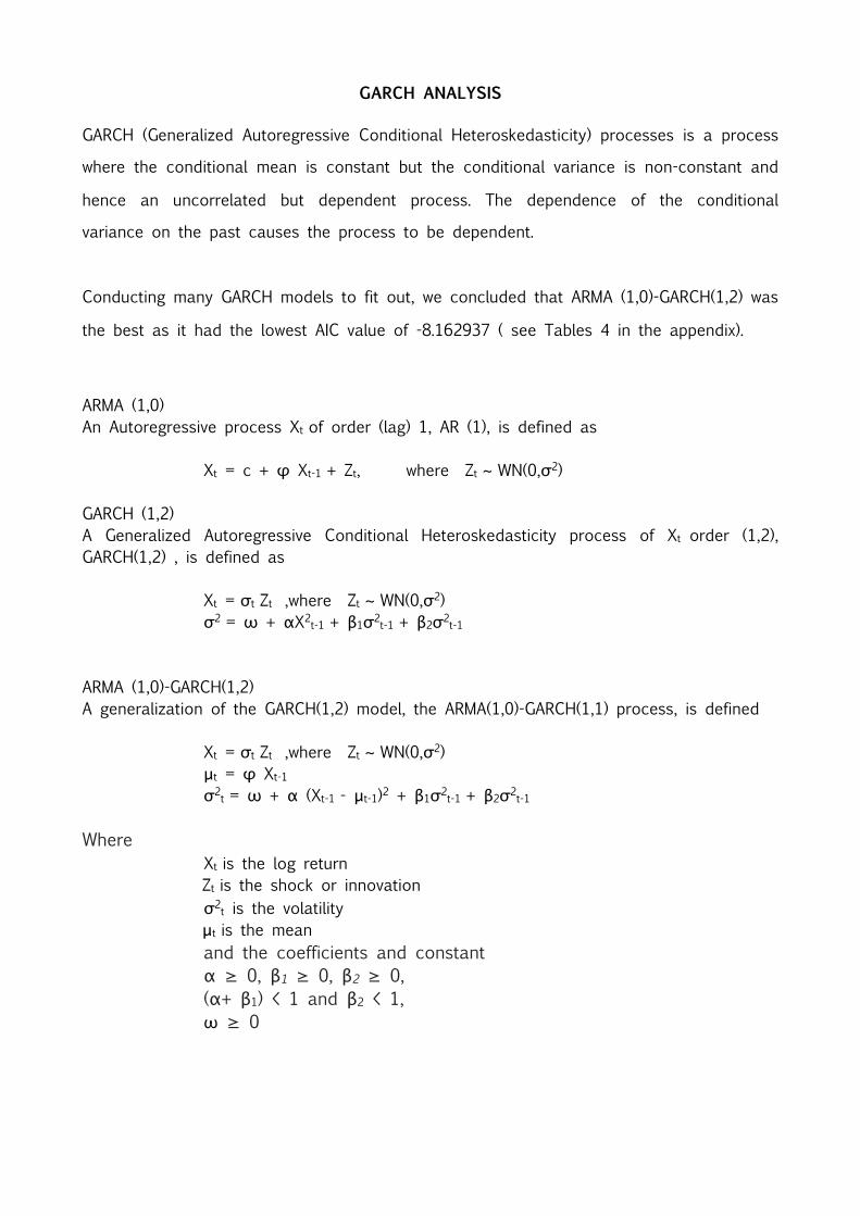
GARCH (Generalized Autoregressive Conditional Heteroskedasticity) processes is a process

where the conditional mean is constant but the conditional variance is non-constant and

hence an uncorrelated but dependent process. The dependence of the conditional

variance on the past causes the process to be dependent.

Conducting many GARCH models to fit out, we concluded that ARMA (1,0)-GARCH(1,2) was

the best as it had the lowest AIC value of -8.162937 ( see Tables 4 in the appendix).

ARMA (1,0)An Autoregressive process Xt of order (lag) 1, AR (1), is defined as

Xt = c + φ Xt-1 + Zt, where Zt ~ WN(0,σ2)

GARCH (1,2)A Generalized Autoregressive Conditional Heteroskedasticity process of Xt order (1,2), GARCH(1,2) , is defined as

Xt = σt Zt ,where Zt ~ WN(0,σ2) σ2 = ω + αX2t-1 + β1σ2t-1 + β2σ2t-1

ARMA (1,0)-GARCH(1,2)A generalization of the GARCH(1,2) model, the ARMA(1,0)-GARCH(1,1) process, is defined

Xt = σt Zt ,where Zt ~ WN(0,σ2) μt = φ Xt-1

σ2t = ω + α (Xt-1 - μt-1)2 + β1σ2t-1 + β2σ2t-1

Where Xt is the log return Zt is the shock or innovation σ2t is the volatility μt is the mean and the coefficients and constant α ≥ 0, β1 ≥ 0, β2 ≥ 0, (α+ β1) < 1 and β2 < 1, ω ≥ 0

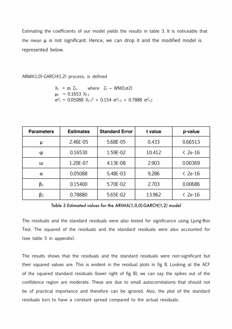
Estimating the coefficients of our model yields the results in table 3. It is noticeable that

the mean μ is not significant. Hence, we can drop it and the modified model is

represented below.

ARMA(1,0)-GARCH(1,2) process, is defined

Xt = σt Zt, where Zt ~ WN(0,σ2) μt = 0.1653 Xt-1

σ2t = 0.05088 Xt-12 + 0.154 σ2t-1 + 0.7888 σ2t-2

Parameters Estimates Standard Error t value p-value

μ 2.46E-05 5.68E-05 0.433 0.66513

φ 0.16530 1.59E-02 10.412 < 2e-16

ω 1.20E-07 4.13E-08 2.903 0.00369

α 0.05088 5.48E-03 9.286 < 2e-16

β1 0.15400 5.70E-02 2.703 0.00686

β2 0.78880 5.65E-02 13.962 < 2e-16

Table 3 Estimated values for the ARIMA(1,0,0)-GARCH(1,2) model

The residuals and the standard residuals were also tested for significance using Ljung-Box

Test. The squared of the residuals and the standard residuals were also accounted for

(see table 5 in appendix).

The results shows that the residuals and the standard residuals were non-significant but

their squared values are. This is evident in the residual plots in fig 8. Looking at the ACF

of the squared standard residuals (lower right of fig 8), we can say the spikes out of the

confidence region are moderate. These are due to small autocorrelations that should not

be of practical importance and therefore can be ignored. Also, the plot of the standard

residuals turn to have a constant spread compared to the actual residuals.

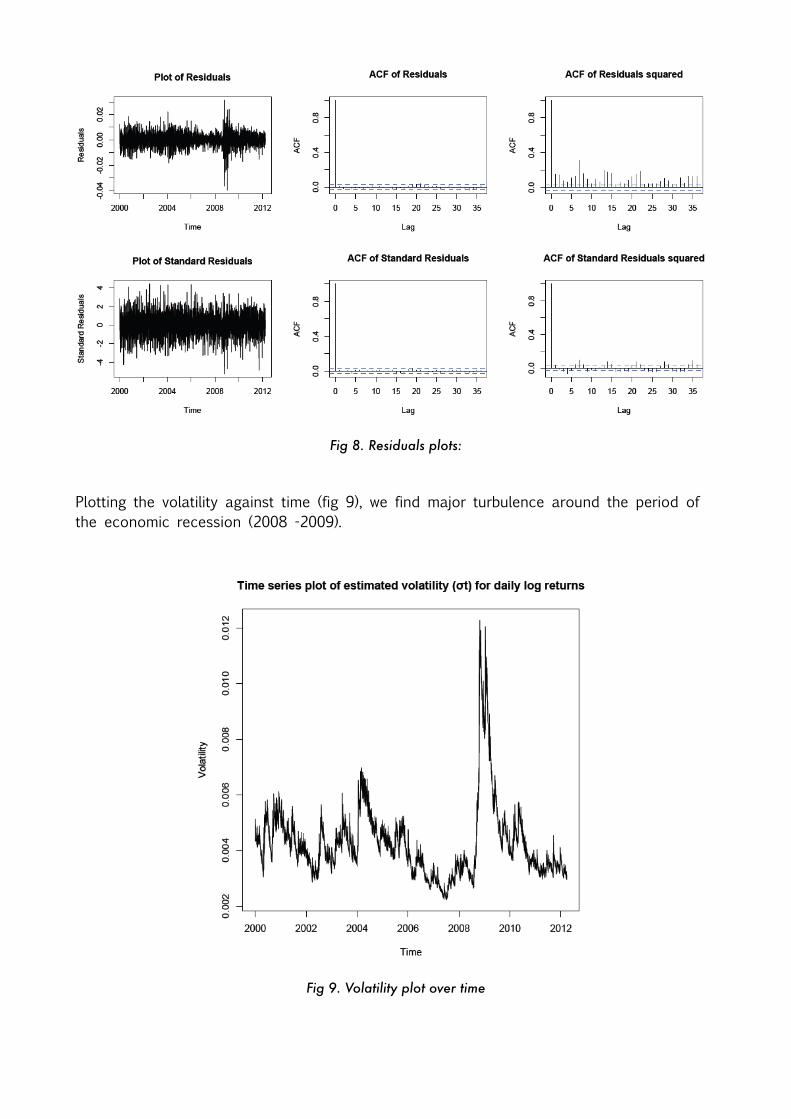
Fig 8. Residuals plots:

Plotting the volatility against time (fig 9), we find major turbulence around the period of the economic recession (2008 -2009).

Fig 9. Volatility plot over time

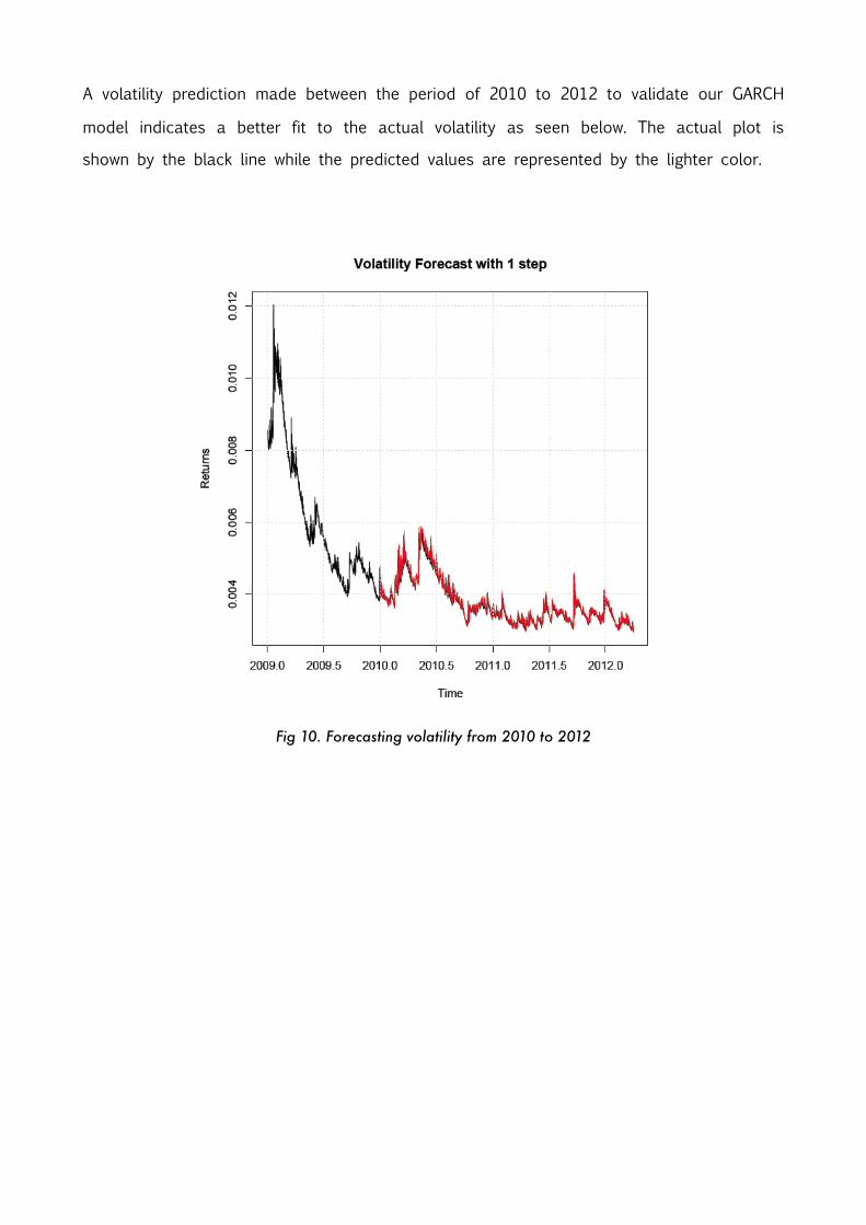
A volatility prediction made between the period of 2010 to 2012 to validate our GARCH

model indicates a better fit to the actual volatility as seen below. The actual plot is

shown by the black line while the predicted values are represented by the lighter color.

Fig 10. Forecasting volatility from 2010 to 2012

INTERPRETATION

To apply the ARMA modeling technique to a time series data, the data should be

stationary. The logarithm of returns of the exchange rates are stationary, as seen in the

ACF plots, thus, the integration part of the ARIMA process is zero.

Volatility in the data was fairly homogeneous from 2000 to 2006 with 2008 to 2012

being inconsistent. This condition makes fitting ARMA to financial data quite difficult. This

was evident in the model orders - MA(1). The ARMA models obtained were not credible

and therefore producing poor prediction outcomes.

Due to the changing variance observed in the series from 2007 to 2010, it was

imperative that we analyze the variance of the series using ARMA(0,1)-GARCH(1,2). This

resulted in a better prediction of the volatility.

CONCLUSION

Time series analysis and modeling is a very popular technique in mathematics and

statistics used to explore the hidden details in time dependent data. ARIMA (ARMA)

modeling is one of the basic time series methods employed in practice. In this study, we

examined the foreign exchange rate between the GBP and the USD. Due the nature of

the data, the logarithms of the returns of the rates are used in the analysis instead of

the actual data. This is due to the favorable statistical properties of the logarithm of the

returns provides for analysis.

As noted previously, ARIMA (ARMA) modeling fails to effectively capture the process being

followed and subsequent forecasting chosen observations for validation. An application of

an alternative modeling technique (ARCH/GARCH) is used be to analyze the volatility in

the series and turn out to be of significant analysis due to the fact that it provides

bankers and traders information about the “value at risk” for a given portfolio.

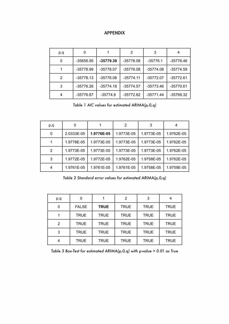
APPENDIX

p,q 0 1 2 3 4

0 -35656.95 -35779.39 -35778.08 -35776.1 -35776.46

1 -35778.99 -35778.07 -35776.08 -35774.08 -35774.59

2 -35778.13 -35776.08 -35774.11 -35772.07 -35772.61

3 -35776.26 -35774.18 -35774.57 -35773.46 -35770.61

4 -35776.87 -35774.8 -35772.82 -35771.44 -35769.32

Table 1 AIC values for estimated ARIMA(p,0,q)

p,q 0 1 2 3 4

0 2.0333E-05 1.9776E-05 1.9773E-05 1.9773E-05 1.9762E-05

1 1.9778E-05 1.9773E-05 1.9773E-05 1.9773E-05 1.9762E-05

2 1.9773E-05 1.9773E-05 1.9773E-05 1.9773E-05 1.9762E-05

3 1.9772E-05 1.9772E-05 1.9762E-05 1.9758E-05 1.9762E-05

4 1.9761E-05 1.9761E-05 1.9761E-05 1.9758E-05 1.9759E-05

Table 2 Standard error values for estimated ARIMA(p,0,q)

p,q 0 1 2 3 4

0 FALSE TRUE TRUE TRUE TRUE

1 TRUE TRUE TRUE TRUE TRUE

2 TRUE TRUE TRUE TRUE TRUE

3 TRUE TRUE TRUE TRUE TRUE

4 TRUE TRUE TRUE TRUE TRUE

Table 3 Box-Test for estimated ARIMA(p,0,q) with p-value > 0.01 as True

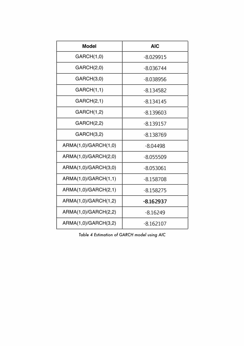
Model AIC

GARCH(1,0) -8.029915

GARCH(2,0) -8.036744

GARCH(3,0) -8.038956

GARCH(1,1) -8.134582

GARCH(2,1) -8.134145

GARCH(1,2) -8.139603

GARCH(2,2) -8.139157

GARCH(3,2) -8.138769

ARMA(1,0)/GARCH(1,0) -8.04498

ARMA(1,0)/GARCH(2,0) -8.055509

ARMA(1,0)/GARCH(3,0) -8.053061

ARMA(1,0)/GARCH(1,1) -8.158708

ARMA(1,0)/GARCH(2,1) -8.158275

ARMA(1,0)/GARCH(1,2) -8.162937

ARMA(1,0)/GARCH(2,2) -8.16249

ARMA(1,0)/GARCH(3,2) -8.162107

Table 4 Estimation of GARCH model using AIC

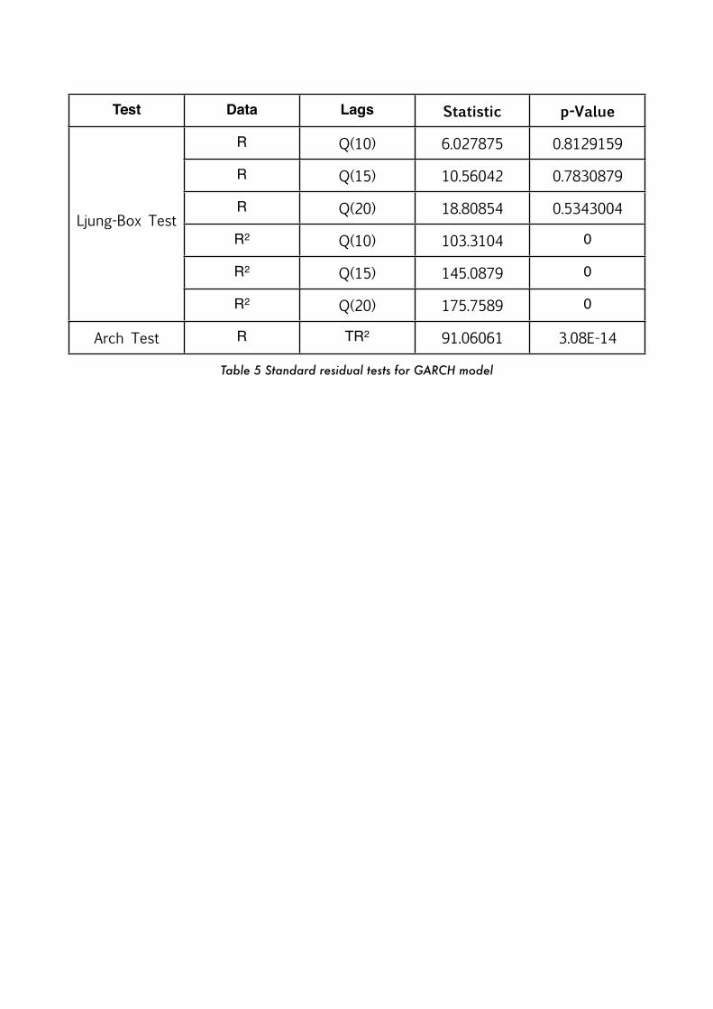
Test Data Lags Statistic p-Value

Ljung-Box Test

R Q(10) 6.027875 0.8129159

Ljung-Box Test

R Q(15) 10.56042 0.7830879

Ljung-Box TestR Q(20) 18.80854 0.5343004

Ljung-Box TestR2 Q(10) 103.3104 0

Ljung-Box Test

R2 Q(15) 145.0879 0

Ljung-Box Test

R2 Q(20) 175.7589 0

Arch Test R TR2 91.06061 3.08E-14

Table 5 Standard residual tests for GARCH model

REFERENCES

• Tsay, Ruey S, (2001), “Analysis of Financial Time Series”, Third Edition

• Chatfield, Chris (2005), “The Analysis of Time Series, An Introduction”, Sixth Edition

• Brockwell, Peter., Davis, Richard.,”Introduction to Time Series and Forecasting”, Second Edition

• Kedem, Benjamin., Fokianos, Konstantinos., (2002)“Regression Models for Time Series Analysis”, Wiley and Sons Inc