Time series modeling of elevatortraffic

Viljami Pirttimaa

School of Engineering

Thesis submitted for examination for the degree of Master ofScience in Technology.Espoo 02.09.2020

Supervisor

Professor Sven Bossuyt

Advisors

D.Sc. (Tech.) Juho Kokkala

D.Sc. (Tech.) Juha-Matti Kuusinen

Copyright © 2020 Viljami Pirttimaa

Aalto University, P.O. BOX 11000, 00076 AALTOwww.aalto.fi

Abstract of the master’s thesis

Author Viljami PirttimaaTitle Time series modeling of elevator trafficMaster programme Mechanical Engineering Code ENG25Supervisor Professor Sven BossuytAdvisors D.Sc. (Tech.) Juho Kokkala, D.Sc. (Tech.) Juha-Matti KuusinenDate 02.09.2020 Number of pages 86 Language EnglishAbstractLarge changes in people flow can happen in buildings throughout their life cycles.This thesis studies long-term forecasting of elevator traffic data using time seriesmodeling. The models can also be used for automatic detection of anomalies, whichmakes it possible to quickly react to unexpected problems. Long-term forecasts canbe used for planning changes to elevator systems before their capacity is exceededand problems in people flow arise.

This thesis includes a literature review of time series characteristics and models.Year-ahead forecasts were made with one traditional and two machine learning-basedmodels, which were chosen based on the literature review. The forecasts obtainedwith the models were compared to a simple baseline model, which is based on theobservations from the previous year. Three models were used for anomaly detection.Their results were evaluated by comparing their findings to known events during thetest period.

The forecasting methods modeled the complex seasonality in the time series well.Predicting the long-term trend in the time series was not as successful with any ofthe models. Based on the results, XGBoost machine learning model turned out tobe the best-performing method. However, the differences between the models weresmall and only data from a single building was used, which makes it impossible togeneralize the result. The anomaly detection models found several days with lessor more traffic than normal. For some of these days, an explanation supporting thefindings of the models could be found.

People flow data can give invaluable insights into how different types of build-ings are used and how people flow changes throughout the lifecycle of each building.Long-term forecasts are helpful especially when elevator modernizations are planned.Anomaly detection is useful for servicing the elevators when problems are detected.Based on the results of this thesis, people flow data should be collected also in thefuture, as it can be a valuable asset.Keywords People flow, time series, forecasting, anomaly detection, machine learning

Aalto-yliopisto, PL 11000, 00076 AALTOwww.aalto.fi

Diplomityön tiivistelmä

Tekijä Viljami PirttimaaTyön nimi Hissiliikenteen aikasarjamallintaminenMaisteriohjelma Konetekniikka Koodi ENG25Työn valvoja Professori Sven BossuytTyön ohjaajat TkT Juho Kokkala, TkT Juha-Matti KuusinenPäivämäärä 02.09.2020 Sivumäärä 86 Kieli EnglantiTiivistelmäRakennusten ihmisvirroissa voi tapahtua suuriakin muutoksia rakennuksen elinkaa-ren aikana. Tämä diplomityö tutkii, voidaanko hissiliikenteen ihmisvirtoja ennustaapitkälle tulevaisuuteen käyttämällä aikasarjojen mallinnusmenetelmiä. Mallit mahdol-listavat myös odottamattomien muutosten automaattisen tunnistamisen, joka nopeut-taa ongelmien korjaamista. Pitkän ajan ennusteilla voidaan suunnitella muutoksiahissijärjestelmiin ennen kuin niiden kapasiteetti ylittyy ja ongelmia ihmisvirroissaalkaa esiintyä.

Tutkimukseen sisältyy kirjallisuuskatsaus aikasarjoihin ja niiden mallinnusmene-telmiin. Vuoden mittaisia ennusteita tehtiin yhdellä perinteisellä ja kahdella koneop-pimiseen perustavalla mallinnusmenetelmällä, jotka valittiin kirjallisuuskatsauksenperusteella. Mallien ennusteita verrattiin yksinkertaiseen verrokkimalliin, joka pe-rustuu edellisvuoden arvoihin. Odottamattomia tapahtumia tunnistettiin kolmellamallilla. Niiden tuloksia arvioitiin vertaamalla mallien löydöksiä tunnettuihin tapah-tumiin testijakson aikana.

Ennustusmallit onnistuivat mallintamaan aikasarjojen monimutkaiset kausivaih-telut hyvin. Sen sijaan pitkän aikavälin trendien ennustamisessa oli ongelmia kaikillamalleilla. Tulosten perusteella XGBoost-koneoppimismalli osoittautui parhaaksi en-nustusmenetelmäksi. Koska erot mallien välillä olivat pieniä ja mallinukseen käytettiinvain yhden rakennuksen dataa, ei tuloksia voida pitää yleispätevinä. Odottamat-tomien tapahtumien tunnistamiseen käytetyt mallit löysivät useita päiviä, joidenliikenne oli pienempää tai suurempaa kuin normaalisti. Osalle näistä päivistä pystyt-tiin löytämään selitys, joka tukee mallien löydöksiä.

Aikasarjamallinnuksen avulla datasta voidaan oppia, miten erilaisten rakennustenihmisvirrat muuttuvat niiden elinkaaren aikana. Pitkän ajan ennusteista on hyötyäetenkin hissien modernisoinnin suunnittelussa, ja poikkeamien tunnistamisesta muunmuassa hissien huoltamisessa. Tulosten perusteella voidaan todeta, että hissiliiken-teen dataa kannattaa kerätä myös tulevaisuudessa, sillä se voi osoittautua erittäinarvokkaaksi.Avainsanat Aikasarja, hissiliikenne, ennustaminen, poikkeamien tunnistaminen,

koneoppiminen

5

PrefaceI want to thank Professor Sven Bossuyt for supervising my thesis. He handled thepractical arrangements from the school’s side so I could focus on working on thethesis. I also want to thank my advisors Juha-Matti Kuusinen and Juho Kokkala.Juha-Matti took care of the arrangements from KONE’s side and made me feel athome while working in his team. Juho guided me through the whole process startingfrom the planning of the topic all the way to the final proofreading. He gave mesome direction to keep the modeling on the right track. His comments on the textwere more thorough and extensive than I could ever had hoped for.

I will also thank my family and friends who have helped me over the years inmy studies. Lastly, I want to thank my girlfriend who has cheered me up andmotivated me to finish this thesis in a timely manner.

Graduation feels like I am leaving a big part of my life in the past, but it alsogives me a great sense of accomplishment. Fortunately, I have had the chance toalready familiarize myself with the working life, so I feel excited about what is waitingfor me in the future.

Espoo, 02.09.2020

Viljami Pirttimaa

6

ContentsAbstract 3

Abstract (in Finnish) 4

Preface 5

Contents 6

Symbols and abbreviations 8

1 Introduction 101.1 Objectives . . . . . . . . . . . . . . . . . . . . . . . . . . . . . . . . . 111.2 Structure . . . . . . . . . . . . . . . . . . . . . . . . . . . . . . . . . 11

2 Literature review 122.1 Time series data . . . . . . . . . . . . . . . . . . . . . . . . . . . . . . 122.2 Properties of time series data . . . . . . . . . . . . . . . . . . . . . . 132.3 Stationarity and unit-root tests . . . . . . . . . . . . . . . . . . . . . 172.4 Transformations and seasonal adjustment . . . . . . . . . . . . . . . . 19

2.4.1 Removing heteroscedasticity . . . . . . . . . . . . . . . . . . . 192.4.2 Removing trend . . . . . . . . . . . . . . . . . . . . . . . . . . 212.4.3 Removing seasonality . . . . . . . . . . . . . . . . . . . . . . . 23

2.5 Time series decomposition . . . . . . . . . . . . . . . . . . . . . . . . 232.6 Imputation . . . . . . . . . . . . . . . . . . . . . . . . . . . . . . . . 272.7 Time series models . . . . . . . . . . . . . . . . . . . . . . . . . . . . 28

2.7.1 Simple models . . . . . . . . . . . . . . . . . . . . . . . . . . . 292.7.2 Model parsimony . . . . . . . . . . . . . . . . . . . . . . . . . 30

2.8 Stochastic models . . . . . . . . . . . . . . . . . . . . . . . . . . . . . 302.8.1 Exponential smoothing (ETS) . . . . . . . . . . . . . . . . . . 312.8.2 Autoregressive models (AR) . . . . . . . . . . . . . . . . . . . 322.8.3 Moving average models (MA) . . . . . . . . . . . . . . . . . . 322.8.4 ARMA, ARIMA and SARIMA models . . . . . . . . . . . . . 332.8.5 Box-Jenkins methodology . . . . . . . . . . . . . . . . . . . . 332.8.6 TBATS . . . . . . . . . . . . . . . . . . . . . . . . . . . . . . 34

2.9 Machine learning . . . . . . . . . . . . . . . . . . . . . . . . . . . . . 342.9.1 Neural networks . . . . . . . . . . . . . . . . . . . . . . . . . . 352.9.2 RNN . . . . . . . . . . . . . . . . . . . . . . . . . . . . . . . . 372.9.3 Long short-term memory (LSTM) . . . . . . . . . . . . . . . . 372.9.4 Decision tree models . . . . . . . . . . . . . . . . . . . . . . . 372.9.5 Random forests . . . . . . . . . . . . . . . . . . . . . . . . . . 402.9.6 Gradient boosting . . . . . . . . . . . . . . . . . . . . . . . . . 40

2.10 Forecasting . . . . . . . . . . . . . . . . . . . . . . . . . . . . . . . . 412.10.1 Producing forecasts with a model . . . . . . . . . . . . . . . . 412.10.2 Evaluating forecast accuracy . . . . . . . . . . . . . . . . . . . 42

7

2.11 Anomaly detection . . . . . . . . . . . . . . . . . . . . . . . . . . . . 44

3 Materials and methods 463.1 Elevator-specific terms and statistics . . . . . . . . . . . . . . . . . . 463.2 Data . . . . . . . . . . . . . . . . . . . . . . . . . . . . . . . . . . . . 463.3 Implications for modeling . . . . . . . . . . . . . . . . . . . . . . . . 503.4 Smart seasonal differencing and smart lag . . . . . . . . . . . . . . . 513.5 Imputing missing values in data . . . . . . . . . . . . . . . . . . . . . 513.6 Forecasting . . . . . . . . . . . . . . . . . . . . . . . . . . . . . . . . 56

3.6.1 Forecasting experiment . . . . . . . . . . . . . . . . . . . . . . 563.6.2 LSTM . . . . . . . . . . . . . . . . . . . . . . . . . . . . . . . 573.6.3 ARIMA with smart seasonal differencing (ASSD) . . . . . . . 593.6.4 XGBoost . . . . . . . . . . . . . . . . . . . . . . . . . . . . . . 60

3.7 Anomaly detection . . . . . . . . . . . . . . . . . . . . . . . . . . . . 623.7.1 AnomalyDetection R package . . . . . . . . . . . . . . . . . . 623.7.2 Rolling average and standard deviation . . . . . . . . . . . . . 633.7.3 ARIMA with smart seasonal differencing (ASSD) . . . . . . . 633.7.4 tsoutliers . . . . . . . . . . . . . . . . . . . . . . . . . . . . . . 64

4 Results 654.1 Forecasting . . . . . . . . . . . . . . . . . . . . . . . . . . . . . . . . 65

4.1.1 LSTM . . . . . . . . . . . . . . . . . . . . . . . . . . . . . . . 684.1.2 ARIMA with smart seasonal differencing . . . . . . . . . . . . 704.1.3 XGBoost . . . . . . . . . . . . . . . . . . . . . . . . . . . . . . 72

4.2 Anomaly detection . . . . . . . . . . . . . . . . . . . . . . . . . . . . 74

5 Discussion 785.1 Forecasting . . . . . . . . . . . . . . . . . . . . . . . . . . . . . . . . 785.2 Anomaly detection . . . . . . . . . . . . . . . . . . . . . . . . . . . . 79

6 Conclusions 81

References 82

8

Symbols and abbreviations

Symbolsα level smoothing parameter in an ETS modelbt trend equation of an ETS model at time tβ trend smoothing parameter an ETS modelc constant leveld order differencing in an ARIMA modelεt Stochastic error term at time tϕi ith order weight of an AR modelγ seasonal smoothing parameter for an ETS modelGi Gini impurity for the ith node of a decision treeh forecast horizonk number of predictors in a model, a constant used for calculationlt level equation of an ETS model at time tλ parameter used in Box-Cox transformationλk kth frequency in harmonic regressionm number of observations per seasonal periodn length of a rolling windowrk sample autocorrelation for lag kσt rolling standard deviation at time tSt seasonal component at time tst seasonal equation of an ETS model at time tt time-step at time tT length of a time seriesTt trend component at time tTDt deterministic component of a time series at time tθi ith order weight of a MA modelp order of an autoregressive modelq order of a moving average modelRt remainder component at time tyt value of time series y at time tyt predicted value of time series y at time ty mean value of time series yy′ differenced time series yzt stochastic component of a time series at time t

OperatorsS(yt) Smart lag value of time series y at time tL(yt) Smart lead value of time series y at time t

9

AbbreviationsACF Autocorrelation FunctionADF Augmented Dickey-FullerAIC Akaike Information CriterionAR Auto RegressiveASSD ARIMA with smart seasonal differencingBIC Schwarz’s Bayesian Information CriterionCART Classification and Regression TreeCT Call TimeDCS Destination Control SystemDNN Deep Neural NetworkDOP Destination Operating PanelESD Extreme Studentized Deviate (ESD) testETS Exponential SmoothingGPU Graphics Processing UnitKPSS Kwiatkowski-Phillips-Schmidt-ShinLOCF Last Observation Carried ForwardLOESS Locally Estimated Scatterplot SmoothingLSTM Long Short-Term MemoryMA Moving AverageMAE Mean Absolute ErrorMAPE Mean Absolute Percentage ErrorMBE Mean Bias ErrorMLE Maximum Likelyhood EstimateNaN Not a NumberNN Neural NetworkNOCB Next Observation Carried BackwardOLS Ordinary Least SquaresPACF Partial Autocorrelation FunctionPP Phillips-PerronRMS Root Mean SquareRMSE Root Mean Square ErrorRNN Recurrent Neural NetworkReLU Rectified Linear UnitS-H-ESD Seasonal Hybrid ESD algorithmSARIMA Seasonal Autoregressive Integraded Moving AverageSTL Seasonal and Treand decomposition using LoessTPU Tensor Processing UnitTTD Time To DestinationWT Waiting Time

1 IntroductionIn modern office buildings it is common to have many tenants which might changethroughout the lifetime of the building. This can have significant impact on thepeople flow of the building and the performance of the elevator system. If there is aconsiderable increase in building population, elevator usage can exceed the originaldesign capacity of the elevator system. This will cause long waiting times and poorperformance during peak traffic times like lunch time [1].

Elevator performance can be improved with modernization. A common approachis to change from a conventional elevator control system to a destination controlsystem (DCS). This can increase the maximum handling capacity by 30 % [1].Performance can be further improved by modernizing the elevator drives to increasetheir speed.

Ordinarily the modernization process is started after the elevator performance hasbecome inadequate. The time frame from noticing the poor performance to addressingthe issue with modernizing can be undesirably long. First the tenants complain tothe building owner, then the building owner complains to the sales department of theelevator company and they inform the department which investigates the problem.If the modernization could be planned before the problems start, it could be done atthe most convenient time like during other renovation. This could save costs andimprove the daily experience of the tenants.

Elevator systems already collect usage data which includes the number of callsand waiting time for each call. This data is invaluable in troubleshooting the causeof poor performance and planning modernizations. This data could also be used forpredicting long-term future traffic demand and automatic detection of temporaryand persistent changes in demand and performance. If problems are expected inthe future, discussions about modernization can be started with the building ownerwell before problems arise. In case the people flow deteriorates unexpectedly, theproblem can be analyzed before the tenants complain to the building owner.

Sometimes poor performance can be caused by something as simple as wrongconfiguration or operation mode after routine service of the elevators. If such issuecould be automatically detected, it could be resolved even before the tenants complainabout poor performance.

Usage patterns of office buildings are highly seasonal [2]. During weekends andholidays there is generally almost no traffic. This can make before-after comparisonsdifficult after modernization. Using the collected usage data, the seasonality can bemodeled, and its effect can be subtracted from the data. This would make before-afteranalyses comparable and the effect of the modernization would be clearer.

Some research, e.g. [3], has been done related to short-term (5-15 minutes ahead)predictions of elevator traffic demand. These predictions are useful in optimization ofelevator control systems. However, little research is available on long-term predictionsof elevator traffic. One possible reason for this is the limited availability of suitabledata. Long-term predictions are common in other fields such as electricity demandwhich has been extensively researched [4, 5]. Applying similar methods to elevatordata should yield interesting results.

11

1.1 ObjectivesThe main objective of this thesis is to develop a suitable time series model for elevatortraffic data. This model should provide long-term forecasts of key people flow metricssuch as number of calls and average waiting time. A good time series model alsomakes it possible to automatically detect anomalies like exceptional events andpersistent changes in the data. While there are many use cases for such a model,studying them is out of scope of this thesis.

The time series models are developed by comparing many existing methods usingreal elevator traffic data provided by KONE Corporation. Comparison betweenthe models is made by measuring their prediction accuracy and anomaly detectioncapability. The models are validated using known events and persisting changes inthe real-world data. Prediction accuracy is evaluated by comparing the forecasts toout-of-sample test and validation data.

Another goal for the model is to extract the seasonality in the elevator traffic. Byfiltering out the seasonality in the data, a better understanding of the trend can beachieved. Deseasonalized data is also useful for comparing the elevator performanceat different points in time.

While the data processing, forecasts and anomaly detection will not be automatedin this thesis, it should be easy to apply the model to the data from differentbuildings. This would enable complete automation of the process in the future. Themodel parameters will likely be different in different types of buildings, but there aremethods to automatically optimize them based on measured data. This means thatmethods which require manual tuning of parameters should be avoided.

1.2 StructureThis thesis is divided to the following chapters:

• Chapter 1 presents the background and main objectives for this thesis.

• Chapter 2 contains a brief literature review of the time series modeling methodsconsidered in this thesis.

• Chapter 3 describes the data and modeling methods used for the time seriesanalysis.

• Chapter 4 outlines the results obtained with the developed models.

• Chapter 5 contains a discussion about the applicability of the chosen methodsand improvement ideas for future research.

• Chapter 6 summarizes the outcome of this thesis.

12

2 Literature reviewThis chapter contains a literature review of the topics that are included in the casestudy part of this thesis. First is a brief introduction to time series data and itsproperties. Second part presents different transformation methods for time series dataand imputation of missing values. Time series modeling and forecasting methods aredescribed in the third part. The last part introduces anomaly detection. A high-leveloverview of the topics is presented in this thesis. For a more thorough theoreticalexplanation, see e.g. [6–12].

2.1 Time series dataTime series data consists of continuous or discrete-time observations of a processor a phenomenon over time. Time series in engineering applications are alwaysdiscrete-time because continuous measurement is not technically possible. Often thedata is sampled at regular intervals to simplify the acquisition and analysis of thedata. Regularly sampled time series data is denoted by yt, t = 1, 2, 3 . . . The data isindexed by t which is the point in time when that data point was sampled [6].

Unlike cross-sectional datasets, time series data has a defined time order. Informa-tion about the measured phenomenon is not only contained in the values themselvesbut also in the way they are arranged [6]. Discrete time series is almost alwaysa representation of a continuous process. This means that every observation iscorrelated to the previous observations in some way. This dependence is measured byautocorrelation. Autocorrelation is a useful property for forecasting, i.e., predictingfuture values of a time series based on the current and previous values [7].

In many time series modeling methods time series are thought as realizations of astochastic process [8]. This means that there is some expected value and a probabilitydistribution for every point in time as well as a joint probability distribution acrossall the samples. The measured time series is interpreted as one realization of thatstochastic process. If the expected value, i.e., mean and the probability distributioncan be modeled, future values can be forecasted with the conditional distributionp(yt|y1, . . . , yt−1). This distribution also gives confidence intervals for the forecast.

Time series data can be divided in two different categories, univariate andmultivariate. Univariate data has only one variable that is changing over time.Multivariate time series has multiple variables that are sampled at the same pointsin time. The different variables in a multivariate time series might have somecorrelation which can help in the modeling process. Although the data used in thisthesis is multivariate, only univariate methods are used in this thesis. Researchingthe modeling of elevator traffic data using multivariate methods could be a gooddirection for future research.

Time series modeling has multiple use cases in engineering. Often fitting asuitable model to the data helps understanding the process that generated the timeseries data. If there is a trend, seasonality or sudden level shifts, they might beexplainable by some external influence on the process. A time series model can alsobe used for filtering out noise in the observations [6]. This is especially useful if the

13

measurements are used for controlling the process that generates the data. One ofthe most widely used applications for time series modeling is forecasting. Modelingthe current and previous observations of the time series, a prediction of future valuescan be achieved.

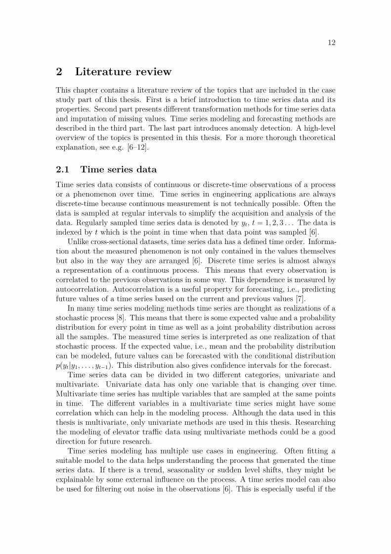
Time series are often visualized with a line plot whose x-axis represents time.One of the oldest time series datasets in existence is the number sunspots per yearshown in Figure 1. The dataset starts from the year 1700 and it is still updated bythe Royal Observatory of Belgium [13]. The data shows some typical properties oftime series data which are discussed in the next Section 2.2.

1720 1770 1820 1870 1920 1970Year

0

50

100

150

Num

ber o

f sun

spot

s

Figure 1: Sunspot data (1700-2008) from the National Geophysical Data Center.

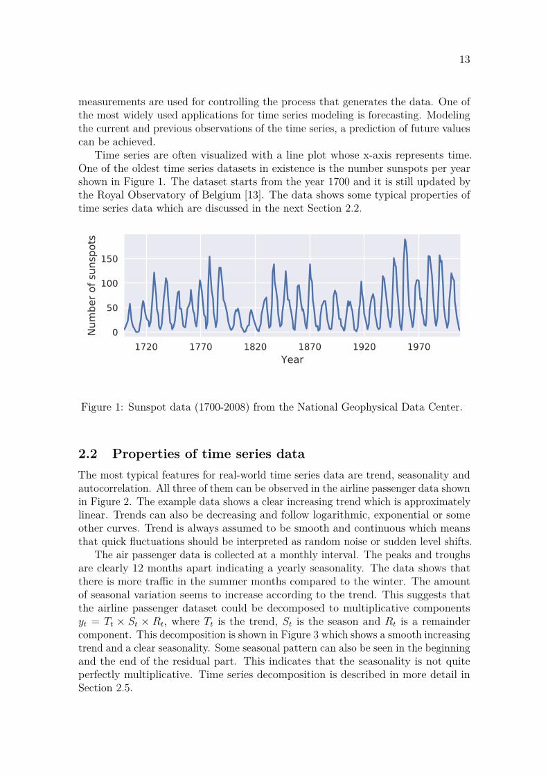
2.2 Properties of time series dataThe most typical features for real-world time series data are trend, seasonality andautocorrelation. All three of them can be observed in the airline passenger data shownin Figure 2. The example data shows a clear increasing trend which is approximatelylinear. Trends can also be decreasing and follow logarithmic, exponential or someother curves. Trend is always assumed to be smooth and continuous which meansthat quick fluctuations should be interpreted as random noise or sudden level shifts.

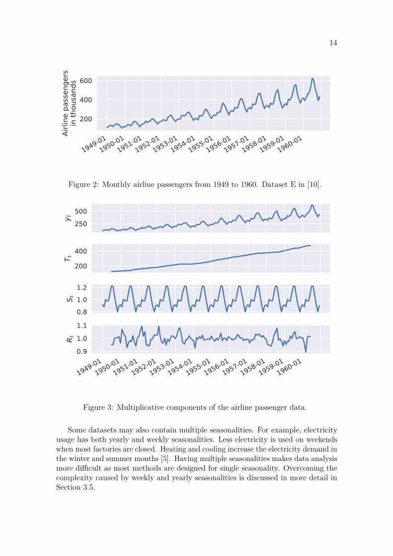
The air passenger data is collected at a monthly interval. The peaks and troughsare clearly 12 months apart indicating a yearly seasonality. The data shows thatthere is more traffic in the summer months compared to the winter. The amountof seasonal variation seems to increase according to the trend. This suggests thatthe airline passenger dataset could be decomposed to multiplicative componentsyt = Tt × St × Rt, where Tt is the trend, St is the season and Rt is a remaindercomponent. This decomposition is shown in Figure 3 which shows a smooth increasingtrend and a clear seasonality. Some seasonal pattern can also be seen in the beginningand the end of the residual part. This indicates that the seasonality is not quiteperfectly multiplicative. Time series decomposition is described in more detail inSection 2.5.

14

1949-011950-01

1951-011952-01

1953-011954-01

1955-011956-01

1957-011958-01

1959-011960-01

200

400

600

Airli

ne p

asse

nger

sin

thou

sand

s

Figure 2: Monthly airline passengers from 1949 to 1960. Dataset E in [10].

250500

y t

200

400

T t

0.81.01.2

S t

1949-011950-01

1951-011952-01

1953-011954-01

1955-011956-01

1957-011958-01

1959-011960-01

0.91.01.1

R t

Figure 3: Multiplicative components of the airline passenger data.

Some datasets may also contain multiple seasonalities. For example, electricityusage has both yearly and weekly seasonalities. Less electricity is used on weekendswhen most factories are closed. Heating and cooling increase the electricity demand inthe winter and summer months [5]. Having multiple seasonalities makes data analysismore difficult as most methods are designed for single seasonality. Overcoming thecomplexity caused by weekly and yearly seasonalities is discussed in more detail inSection 3.5.

15

Autocorrelation measures the correlation of a time series to its past values. It isanalogous to ordinary correlation which measures the linear relationship between twodifferent variables. Autocorrelation coefficient r1 measures the correlation betweenthe current value yt and the value lagged by one observation yt−1. Autocorrelation isa theoretical feature of the stochastic process that generated the time series data.It cannot be calculated with the sampled data but it can be estimated using thesamples. Sample autocorrelation for lag k is calculated as follows:

rk =

T∑t=k+1

(yt − y)(yt−k − y)T∑

t=1(yt − y)2

, (1)

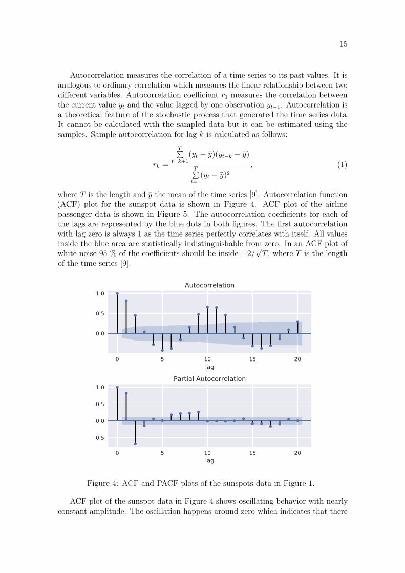
where T is the length and y the mean of the time series [9]. Autocorrelation function(ACF) plot for the sunspot data is shown in Figure 4. ACF plot of the airlinepassenger data is shown in Figure 5. The autocorrelation coefficients for each ofthe lags are represented by the blue dots in both figures. The first autocorrelationwith lag zero is always 1 as the time series perfectly correlates with itself. All valuesinside the blue area are statistically indistinguishable from zero. In an ACF plot ofwhite noise 95 % of the coefficients should be inside ±2/

√T , where T is the length

of the time series [9].

0 5 10 15 20lag

0.0

0.5

1.0Autocorrelation

0 5 10 15 20lag

0.5

0.0

0.5

1.0Partial Autocorrelation

Figure 4: ACF and PACF plots of the sunspots data in Figure 1.

ACF plot of the sunspot data in Figure 4 shows oscillating behavior with nearlyconstant amplitude. The oscillation happens around zero which indicates that there

16

0 5 10 15 20 25 30lag

0.5

0.0

0.5

1.0Autocorrelation

0 5 10 15 20 25 30lag

0.5

0.0

0.5

1.0Partial Autocorrelation

Figure 5: ACF and PACF plots of the airline passenger data in Figure 2.

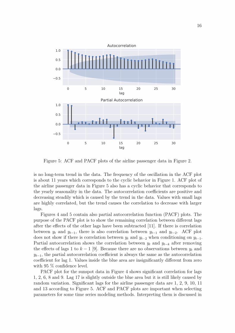
is no long-term trend in the data. The frequency of the oscillation in the ACF plotis about 11 years which corresponds to the cyclic behavior in Figure 1. ACF plot ofthe airline passenger data in Figure 5 also has a cyclic behavior that corresponds tothe yearly seasonality in the data. The autocorrelation coefficients are positive anddecreasing steadily which is caused by the trend in the data. Values with small lagsare highly correlated, but the trend causes the correlation to decrease with largerlags.

Figures 4 and 5 contain also partial autocorrelation function (PACF) plots. Thepurpose of the PACF plot is to show the remaining correlation between different lagsafter the effects of the other lags have been subtracted [11]. If there is correlationbetween yt and yt−1, there is also correlation between yt−1 and yt−2. ACF plotdoes not show if there is correlation between yt and yt−2 when conditioning on yt−1.Partial autocorrelation shows the correlation between yt and yt−k after removingthe effects of lags 1 to k − 1 [9]. Because there are no observations between yt andyt−1, the partial autocorrelation coefficient is always the same as the autocorrelationcoefficient for lag 1. Values inside the blue area are insignificantly different from zerowith 95 % confidence level.

PACF plot for the sunspot data in Figure 4 shows significant correlation for lags1, 2, 6, 8 and 9. Lag 17 is slightly outside the blue area but it is still likely caused byrandom variation. Significant lags for the airline passenger data are 1, 2, 9, 10, 11and 13 according to Figure 5. ACF and PACF plots are important when selectingparameters for some time series modeling methods. Interpreting them is discussed in

17

more detail in Section 2.8 where AR and MA models are introduced.

2.3 Stationarity and unit-root testsMost statistical forecasting methods assume time series to be stationary. Stationaritymeans that the statistical properties of the process do not change over time. Morespecifically for a stationary time series yt, the distribution of (yt, . . . , yt+s) does notdepend on t [9]. This implies that the mean and standard deviation of the time seriesstay constant over time. A classic example of a stationary time series is white noise.It contains all frequencies with the same amplitude and as such it looks statisticallythe same at all points in time. White noise is independent and identically distributed(i.i.d.), which means that it does not have autocorrelation. However, stationary timeseries can have autocorrelation, as long as it does not change over time.

Variance that changes over time is one of the common features in real-world timeseries that make them non-stationary. In literature, it is called heteroscedasticity.This behavior is clearly visible in the observed data yt in Figure 2.

Stationarity of time series can be tested with multiple methods. The simplestmethod is to divide the time series to two or more parts and calculate the mean andvariance for each of the sections. If the statistical properties for all the parts aresimilar, the time series can probably be assumed to be stationary. However, thisnaïve method does not detect things like cyclic behavior. To understand methodsdesigned for this task, a brief overview of unit root processes is required.

Without going to too much mathematical detail about unit root processes, timeseries can be divided to three categories. Those for which all roots are under 1 arestationary and their stochastic behavior stays the same over time. Random noisemight nudge the mean and variation temporarily, but they tend to get back to theoriginal level. Processes which contain at least one root that is larger than one, areexplosive in their nature [12]. Their variance increases over time and it tends toinfinity.

An edge case between these processes is a unit root process which has at least oneroot equal to one but no roots more than one. Their level drifts randomly with thenoise and their variance tends to infinity [12]. Unit root processes can be modeledwith a random walk model in which each time period adds a random noise to theprevious value. Over long time periods the accumulated error has a mean of zero, butits variance increases. A random nudge caused by the error term causes a persistingchange in the level which does not tend back to the original level.

As an example the first order autoregressive process, yt = a1yt−1 + εt has a unitroot when a1 = 1 [11]. In that case the model becomes a random walk whose levelfluctuates randomly with the εt term. As the effect of past random errors is notdiminished by a1, the errors accumulate, and the stochastic properties of the timeseries change over time. This is illustrated in Figure 6 which shows a stationary andunit-root first order autoregressive processes. The error term εt is the same for bothprocesses. It is sampled from a normal distribution with zero mean and standarddeviation of 1. At t = 20 the error term was set to -10 to nudge both time seriesstrongly downwards. The effect of the nudge is permanent for the unit root process

18

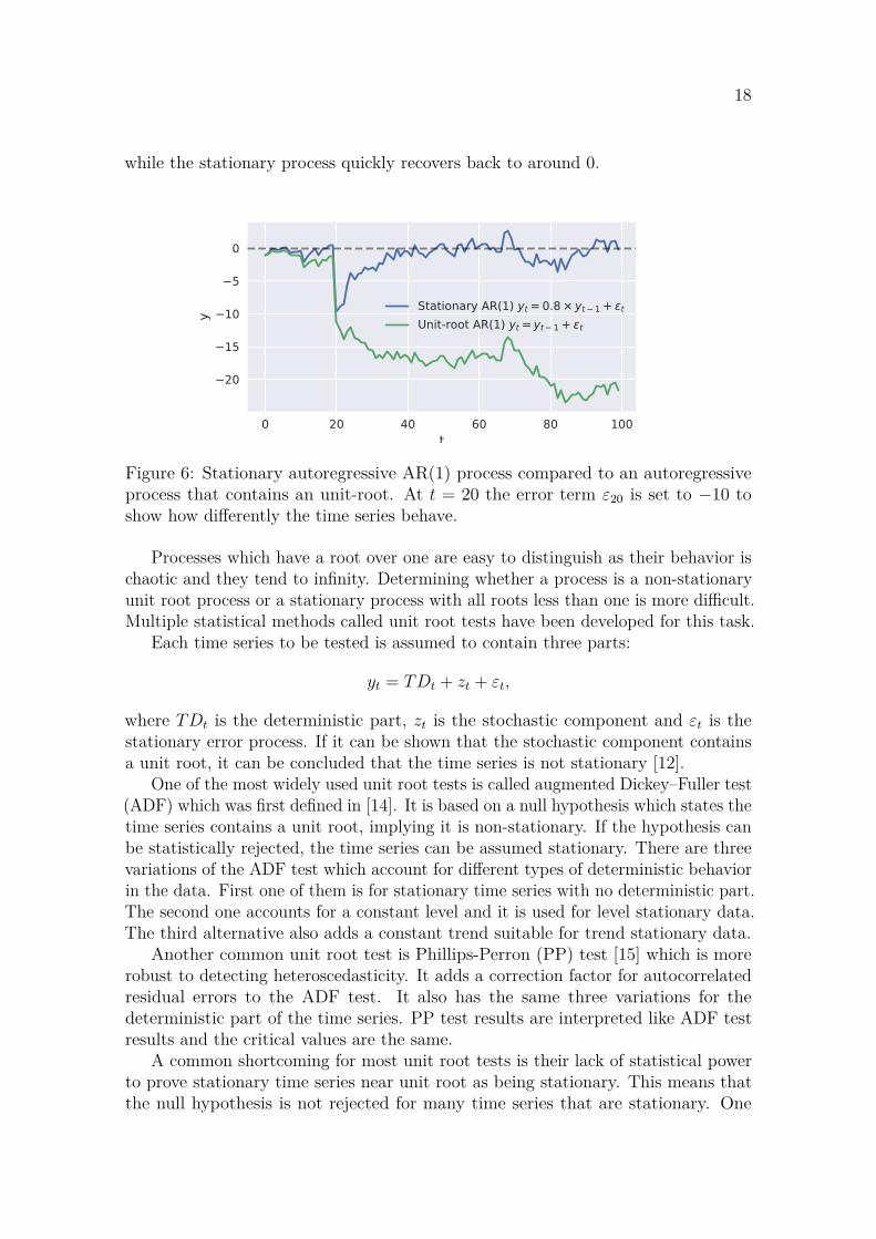
while the stationary process quickly recovers back to around 0.

0 20 40 60 80 100t

20

15

10

5

0

y Stationary AR(1) yt = 0.8 × yt 1 + t

Unit-root AR(1) yt = yt 1 + t

Figure 6: Stationary autoregressive AR(1) process compared to an autoregressiveprocess that contains an unit-root. At t = 20 the error term ε20 is set to −10 toshow how differently the time series behave.

Processes which have a root over one are easy to distinguish as their behavior ischaotic and they tend to infinity. Determining whether a process is a non-stationaryunit root process or a stationary process with all roots less than one is more difficult.Multiple statistical methods called unit root tests have been developed for this task.

Each time series to be tested is assumed to contain three parts:

yt = TDt + zt + εt,

where TDt is the deterministic part, zt is the stochastic component and εt is thestationary error process. If it can be shown that the stochastic component containsa unit root, it can be concluded that the time series is not stationary [12].

One of the most widely used unit root tests is called augmented Dickey–Fuller test(ADF) which was first defined in [14]. It is based on a null hypothesis which states thetime series contains a unit root, implying it is non-stationary. If the hypothesis canbe statistically rejected, the time series can be assumed stationary. There are threevariations of the ADF test which account for different types of deterministic behaviorin the data. First one of them is for stationary time series with no deterministic part.The second one accounts for a constant level and it is used for level stationary data.The third alternative also adds a constant trend suitable for trend stationary data.

Another common unit root test is Phillips-Perron (PP) test [15] which is morerobust to detecting heteroscedasticity. It adds a correction factor for autocorrelatedresidual errors to the ADF test. It also has the same three variations for thedeterministic part of the time series. PP test results are interpreted like ADF testresults and the critical values are the same.

A common shortcoming for most unit root tests is their lack of statistical powerto prove stationary time series near unit root as being stationary. This means thatthe null hypothesis is not rejected for many time series that are stationary. One

19

cause for this is the fact that unit root tests do not handle structural changes in thedata like a change in trend or level [12].

In addition to these unit root tests a different type of statistical test calledKwiatkowski-Phillips-Schmidt-Shin (KPSS) is introduced in [16]. It inverts the nullhypothesis of the ADF meaning that the time series is assumed stationary unlessotherwise statistically proven. It tends to work better for time series that are nearunit root. Interpreting KPSS test results is inverted compared to ADF. KPSS teststatistic indicates stationarity if it is larger than the critical value in Table 1 in [16].

While the implementation details of these tests are not relevant in the scope ofthis thesis, these tests can be quite easily used. They are implemented in multiplesoftware packages like the forecast [17] package for R and statsmodels [18] library forPython. It is important to keep in mind that the tests are statistical and as suchtheir results might contradict each other. A good approach to analyzing stationarityof a time series is to use multiple tests and compare their results critically. Failingone of the tests does not automatically mean the time series is non-stationary, but ifmost of the tests indicate so, that is probably the case. A good approach is to utilizethe opposing hypothesis of the ADF and KPSS tests. If their results contradict, thestrength of the evidence, i.e. p-values of the tests, can be compared.

Many real-world time series datasets contain features that make them non-stationary. Methods that require stationarity can still be utilized, as there aremultiple ways to transform the data so that it becomes weakly stationary. Thesemethods are described in the next Section 2.4.

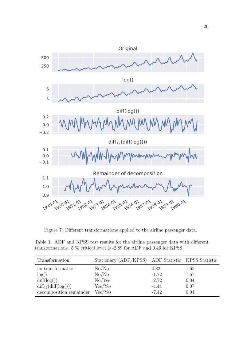
2.4 Transformations and seasonal adjustmentAs discussed earlier, many real-world datasets contain features that make themnon-stationary and difficult to model. These issues can often be overcome withthe help of transformations. Different transformations can be utilized for handlingdifferent properties, and they can be combined to enable the modeling of almostany time series. Most common transformations and adjustments are discussed inthis section. Airline passenger data from Section 2.2 is used as an example datasetto look at the effect of transformations in [7]. It is also used in Figure 7, whichshows the data with different transformations. Table 1 summarizes ADF and KPSSstationary test results of the transformed data.

2.4.1 Removing heteroscedasticity

A common issue with datasets is heteroscedasticity, i.e., variance that changes overtime. This behavior can be seen in the first panel of Figure 7. A widely used methodfor minimizing heteroscedasticity is a simple logarithmic transform wt = log(yt),where wt is the transformed series [7]. As can be seen in the second panel of Figure 7,it stabilizes the variance while leaving the trend and seasonality intact. Logarithmictransform changes the scale of the data completely, but it is not an issue. Transformeddata can be scaled back to the original with the inverse transform yt = ewt . The trendstill persists after the transformation, which causes the data to be non-stationary

20

250500

Original

5

6

log()

0.20.00.2

diff(log())

0.10.00.1

diff12(diff(log()))

1949-011950-01

1951-011952-01

1953-011954-01

1955-011956-01

1957-011958-01

1959-011960-01

0.9

1.0

1.1Remainder of decomposition

Figure 7: Different transformations applied to the airline passenger data.

Table 1: ADF and KPSS test results for the airline passenger data with differenttransformations. 5 % critical level is -2.89 for ADF and 0.46 for KPSS.

Transformation Stationary (ADF/KPSS) ADF Statistic KPSS Statisticno transformation No/No 0.82 1.65log() No/No -1.72 1.67diff(log()) No/Yes -2.72 0.04diff12(diff(log())) Yes/Yes -4.44 0.07decomposition remainder Yes/Yes -7.42 0.04

21

according to both the ADF and KPSS tests. Logarithmic transform is also useful forconstraining modeled values to be positive as the back-transformation produces onlynon-negative values. It is important to keep in mind that log transformation cannotbe used if the data contains negative values.

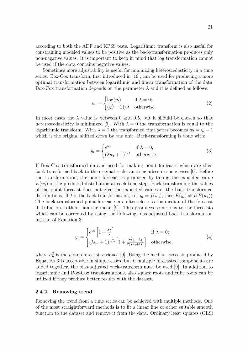
Sometimes more adjustability is useful for minimizing heteroscedasticity in a timeseries. Box-Cox transform, first introduced in [19], can be used for producing a moreoptimal transformation between logarithmic and linear transformation of the data.Box-Cox transformation depends on the parameter λ and it is defined as follows:

wt =

⎧⎨⎩log(yt) if λ = 0;(yλ

t − 1)/λ otherwise.(2)

In most cases the λ value is between 0 and 0.5, but it should be chosen so thatheteroscedasticity is minimized [9]. With λ = 0 the transformation is equal to thelogarithmic transform. With λ = 1 the transformed time series becomes wt = yt − 1which is the original shifted down by one unit. Back-transforming is done with:

yt =

⎧⎨⎩ewt if λ = 0;(λwt + 1)1/λ otherwise.

(3)

If Box-Cox transformed data is used for making point forecasts which are thenback-transformed back to the original scale, an issue arises in some cases [9]. Beforethe transformation, the point forecast is produced by taking the expected valueE(wt) of the predicted distribution at each time step. Back-transforming the valuesof the point forecast does not give the expected values of the back-transformeddistributions. If f is the back-transformation, i.e. yt = f(wt), then E(yt) = f(E(wt)).The back-transformed point forecasts are often close to the median of the forecastdistribution, rather than the mean [9]. This produces some bias to the forecastswhich can be corrected by using the following bias-adjusted back-transformationinstead of Equation 3:

yt =

⎧⎪⎪⎨⎪⎪⎩ewt

[1 + σ2

h

2

]if λ = 0;

(λwt + 1)1/λ

[1 + σ2

h(1−λ)2(λwt+1)2

]otherwise,

(4)

where σ2h is the h-step forecast variance [9]. Using the median forecasts produced by

Equation 3 is acceptable in simple cases, but if multiple forecasted components areadded together, the bias-adjusted back-transform must be used [9]. In addition tologarithmic and Box-Cox transformations, also square roots and cube roots can beutilized if they produce better results with the dataset.

2.4.2 Removing trend

Removing the trend from a time series can be achieved with multiple methods. Oneof the most straightforward methods is to fit a linear line or other suitable smoothfunction to the dataset and remove it from the data. Ordinary least squares (OLS)

22

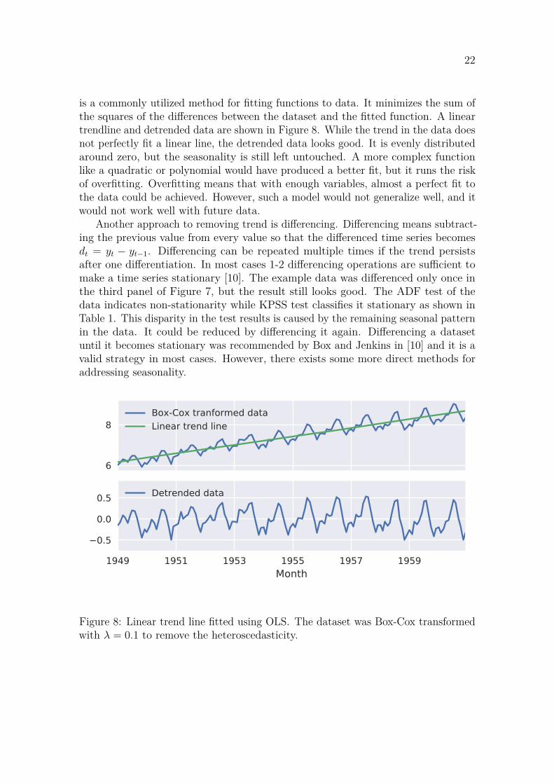
is a commonly utilized method for fitting functions to data. It minimizes the sum ofthe squares of the differences between the dataset and the fitted function. A lineartrendline and detrended data are shown in Figure 8. While the trend in the data doesnot perfectly fit a linear line, the detrended data looks good. It is evenly distributedaround zero, but the seasonality is still left untouched. A more complex functionlike a quadratic or polynomial would have produced a better fit, but it runs the riskof overfitting. Overfitting means that with enough variables, almost a perfect fit tothe data could be achieved. However, such a model would not generalize well, and itwould not work well with future data.

Another approach to removing trend is differencing. Differencing means subtract-ing the previous value from every value so that the differenced time series becomesdt = yt − yt−1. Differencing can be repeated multiple times if the trend persistsafter one differentiation. In most cases 1-2 differencing operations are sufficient tomake a time series stationary [10]. The example data was differenced only once inthe third panel of Figure 7, but the result still looks good. The ADF test of thedata indicates non-stationarity while KPSS test classifies it stationary as shown inTable 1. This disparity in the test results is caused by the remaining seasonal patternin the data. It could be reduced by differencing it again. Differencing a datasetuntil it becomes stationary was recommended by Box and Jenkins in [10] and it is avalid strategy in most cases. However, there exists some more direct methods foraddressing seasonality.

6

8Box-Cox tranformed dataLinear trend line

1949 1951 1953 1955 1957 1959Month

0.5

0.0

0.5 Detrended data

Figure 8: Linear trend line fitted using OLS. The dataset was Box-Cox transformedwith λ = 0.1 to remove the heteroscedasticity.

23

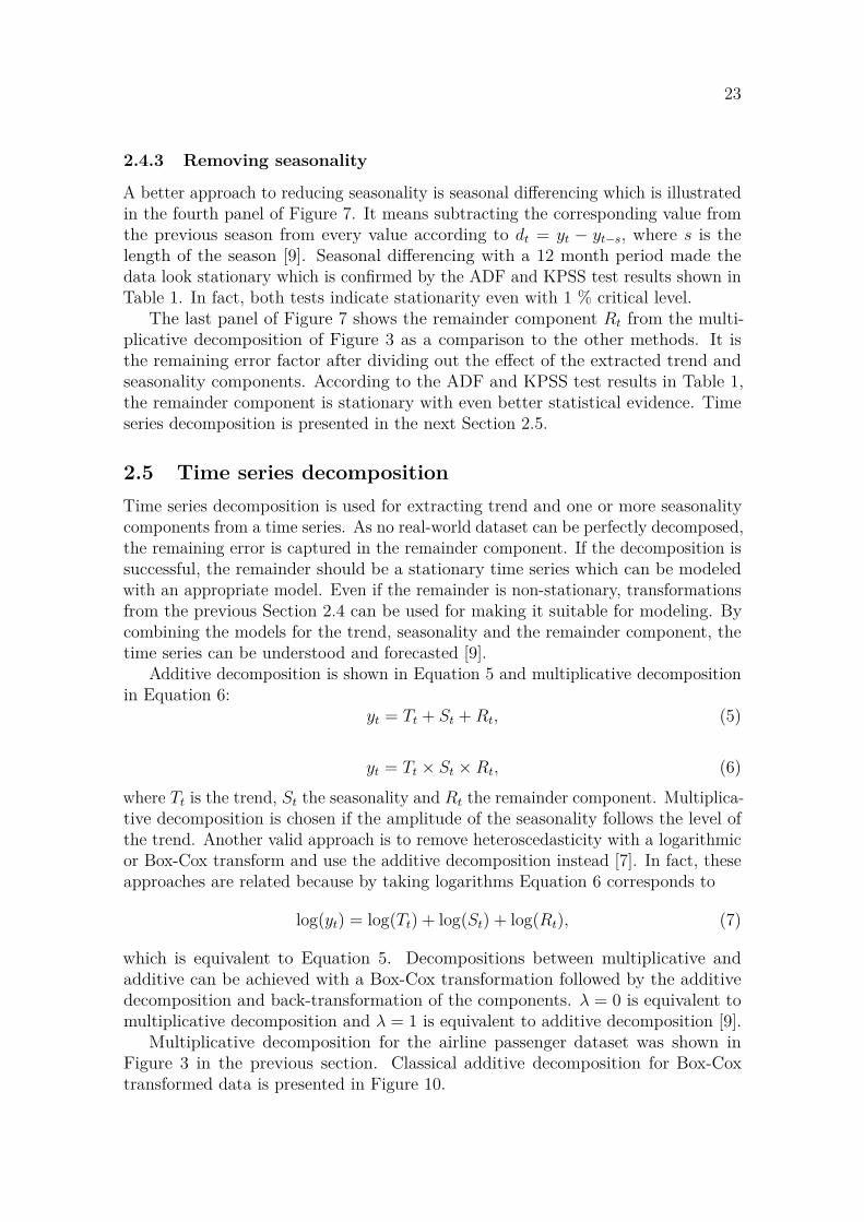
2.4.3 Removing seasonality

A better approach to reducing seasonality is seasonal differencing which is illustratedin the fourth panel of Figure 7. It means subtracting the corresponding value fromthe previous season from every value according to dt = yt − yt−s, where s is thelength of the season [9]. Seasonal differencing with a 12 month period made thedata look stationary which is confirmed by the ADF and KPSS test results shown inTable 1. In fact, both tests indicate stationarity even with 1 % critical level.

The last panel of Figure 7 shows the remainder component Rt from the multi-plicative decomposition of Figure 3 as a comparison to the other methods. It isthe remaining error factor after dividing out the effect of the extracted trend andseasonality components. According to the ADF and KPSS test results in Table 1,the remainder component is stationary with even better statistical evidence. Timeseries decomposition is presented in the next Section 2.5.

2.5 Time series decompositionTime series decomposition is used for extracting trend and one or more seasonalitycomponents from a time series. As no real-world dataset can be perfectly decomposed,the remaining error is captured in the remainder component. If the decomposition issuccessful, the remainder should be a stationary time series which can be modeledwith an appropriate model. Even if the remainder is non-stationary, transformationsfrom the previous Section 2.4 can be used for making it suitable for modeling. Bycombining the models for the trend, seasonality and the remainder component, thetime series can be understood and forecasted [9].

Additive decomposition is shown in Equation 5 and multiplicative decompositionin Equation 6:

yt = Tt + St + Rt, (5)

yt = Tt × St × Rt, (6)

where Tt is the trend, St the seasonality and Rt the remainder component. Multiplica-tive decomposition is chosen if the amplitude of the seasonality follows the level ofthe trend. Another valid approach is to remove heteroscedasticity with a logarithmicor Box-Cox transform and use the additive decomposition instead [7]. In fact, theseapproaches are related because by taking logarithms Equation 6 corresponds to

log(yt) = log(Tt) + log(St) + log(Rt), (7)

which is equivalent to Equation 5. Decompositions between multiplicative andadditive can be achieved with a Box-Cox transformation followed by the additivedecomposition and back-transformation of the components. λ = 0 is equivalent tomultiplicative decomposition and λ = 1 is equivalent to additive decomposition [9].

Multiplicative decomposition for the airline passenger dataset was shown inFigure 3 in the previous section. Classical additive decomposition for Box-Coxtransformed data is presented in Figure 10.

24

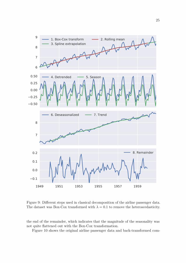
Classical decomposition is achieved with the steps visualized in Figure 9. Firstthe data is transformed to be more compatible with the decomposition model if it isnecessary. In this case a Box-Cox transform with λ = 0.1 was used for removing theincreasing amplitude of the seasonality. The second step is to apply a rolling averagefilter to the data to smooth out noise and seasonality. Rolling average with a laggingwindow is defined as:

yt = 1n

(yt−n + yt−n+1 + · · · + yt) , (8)

where n is the length of the rolling window. The window can be also centeredaround the current time step t, which ensures that the smoothed time series doesnot lag behind the original data. Window length of 2 times the season length isusually appropriate [9]. In this case a two-year window, i.e. 24-month window, wasused which is visualized in red in the first panel of Figure 9. A centered window,i.e. averaging the values from the preceding and following years, was used so thatthe smoothed data does not lag behind the original data. This leaves the first andlast year of data without values as they cannot be calculated. This was fixed byextrapolating the missing values using splines fitted with OLS as shown in Figure 9.

The second panel of Figure 9 shows the detrended data and the season componentcalculated from it. The detrended data is calculated by subtracting the smoothedtrend component from the transformed data. The resulting time series oscillatesaround zero but is has no discernable trend. The seasonality component is calculatedby averaging the corresponding observations from each season [9]. In this case, theaverage value for each month was calculated. It is important that the seasonalitycomponent does not affect the level of the time series over time. This is achieved byensuring the sum of the seasonal component is zero over each season. To accomplishthis, k is subtracted from each seasonal component Si:

k =m∑

i=1Si, (9)

where m is the number of observations per seasonal period. The result in this case wasan average value for every month of the year, which was then repeated through-outthe dataset.

The next steps are deseasonalizing the transformed data and finding the trendcomponent. These steps are visualized in the third panel of Figure 9. The deseason-alized data is produced by subtracting the seasonality component produced in theprevious steps from the original data. This leaves a dataset that shows the trend withsome noise. The trend component is then estimated with a rolling average whosewindow size can be chosen independently from the season. If forecasts are madebased on the decomposition, it could be beneficial to model the trend componentwith an OLS-fitted function instead, as it can be easily extrapolated into the future.In this case a similar rolling average with a 24-month window was chosen.

The last panel of Figure 9 shows the remainder component of the decomposition.It is calculated by subtracting the trend and seasonality components from thetransformed original data. Some seasonal pattern is still visible in the beginning and

25

6

7

8

9 1. Box-Cox transform3. Spline extrapolation

2. Rolling mean

0.50

0.25

0.00

0.25

0.50 4. Detrended 5. Season

7

8

6. Deseasonalized 7. Trend

1949 1951 1953 1955 1957 1959

0.1

0.0

0.1

0.2 8. Remainder

Figure 9: Different steps used in classical decomposition of the airline passenger data.The dataset was Box-Cox transformed with λ = 0.1 to remove the heteroscedasticity.

the end of the remainder, which indicates that the magnitude of the seasonality wasnot quite flattened out with the Box-Cox transformation.

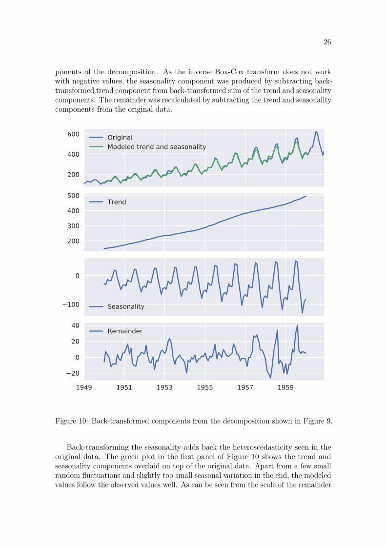
Figure 10 shows the original airline passenger data and back-transformed com-

26

ponents of the decomposition. As the inverse Box-Cox transform does not workwith negative values, the seasonality component was produced by subtracting back-transformed trend component from back-transformed sum of the trend and seasonalitycomponents. The remainder was recalculated by subtracting the trend and seasonalitycomponents from the original data.

200

400

600 OriginalModeled trend and seasonality

200

300

400

500Trend

100

0

Seasonality

1949 1951 1953 1955 1957 1959

20

0

20

40Remainder

Figure 10: Back-transformed components from the decomposition shown in Figure 9.

Back-transforming the seasonality adds back the heteroscedasticity seen in theoriginal data. The green plot in the first panel of Figure 10 shows the trend andseasonality components overlaid on top of the original data. Apart from a few smallrandom fluctuations and slightly too small seasonal variation in the end, the modeledvalues follow the observed values well. As can be seen from the scale of the remainder

27

component, the errors are quite small compared to the scale of the original data. ADFand KPSS tests indicate that the remainder component of the classical decompositionis stationary.

While the classical decomposition is easy to understand and implement, it isnot ideal for all datasets. Estimating the trend using a rolling average tends tosmooth out rapid fluctuations in the data [9]. Calculating the seasonal componentby averaging the values from every season does not allow the season to change overtime. Outliers in the data can be very detrimental in calculating the season becausethere is usually quite few datapoints to average.

A widely used method for decomposition is Seasonal and Trend decompositionusing LOESS (STL) which was first introduced in [20]. LOESS stands for locallyestimated scatterplot smoothing, and it is a more advanced method for estimatingnon-linear relationships. STL decomposition overcomes many of the shortcomingsof classical decomposition. It handles sudden changes in trend better, it supportschanging seasonality and it has a robust method for handling outliers in the data [9].

While the implementation details of STL decomposition are not relevant in thisthesis, it can be easily utilized with software packages like forecast [17] for R andstatsmodels [18] for Python. The forecast package includes a variation called mstlwhich supports multiple seasonalities. This is especially useful for daily data whichcan have both weekly and yearly seasonalities.

2.6 ImputationReal-world time series datasets may contain missing values that can make model-ing and forecasting more difficult. Some modeling methods cannot be used withincomplete data. Missing data can be caused by human or technical errors that areunavoidable in some cases. The issues caused by missing data can be mitigated byfilling the missing values with estimated values. This process is called imputationand it can be implemented in several ways.

Imputation is a common task in many fields of statistics and many implementationsexist in statistical software packages like R. However, most of the methods cannotbe directly applied to univariate time series data as they rely on the correlation ofmultiple variables in a cross-sectional dataset [21]. A univariate time series has onlyone variable which has a time dependence to itself.

The simplest methods for time series imputation include filling the missing valueswith some constant value, e.g., zero or the average of the available data. While thismakes it possible to use modeling methods that require complete data, the imputedvalues might bias the model significantly. Filling the missing values with a constantignores the time dependent nature of the data completely and thus does not utilizeall the information available. In the terminology of Moritz et al. [21]., these types ofimputation methods are called univariate algorithms.

Univariate time series algorithms are specifically designed for imputing time seriesdata and they account for the time dependence of the data [21]. One of the simplestsuch approaches is last observation carried forward (LOCF), i.e., copying the lastknown value to the missing values. Another similar approach is next observation

28

carried backward (NOCB) which means copying the next known value to the missingvalues. These methods work better than the univariate algorithms if the level of thetime series changes over time and the time series has autocorrelation. However, theydo not properly account for trend or seasonality.

Interpolating the missing values using surrounding data is a simple method thataccounts for a trend in the data. Handling seasonality requires more advancedmethods like deseasonalizing the data using decomposition, imputing the values withlinear interpolation and adding the seasonality back in. Another approach is to groupthe data according to the seasonality and interpolate using the corresponding valuesfrom each season.

The third category of methods is called multivariate algorithms with lagged data[21]. Imputation methods not directly suitable for univariate data can be utilizedby creating multiple variables from different lags of the time series. This way thetime dependence of the data can be utilized with algorithms that are not designedfor time series data.

Moritz et al. [21] found univariate time series algorithms to perform the best.Multivariate algorithms with lagged data performed moderately as well but thesimplest univariate methods showed poor performance. Bokde et al. [22] developed anew method to compete with the simpler univariate time series methods. It is basedon Pattern Sequence Forecasting (PSF) which was first proposed by Martínez-Álvarezet al. [23]. In the first step, different types of patterns are searched for from thetime series. In the second step, missing gaps of data are forecasted with the PSFmethod using the data before the gap and backcasted using the data after the gap.Imputed values are the average of the forecast and the backcast. This functionalityis implemented in the imputePSF R package [24].

According to Bokde et al. the imputePSF method performs equally well or bettercompared other univariate time series imputation methods. It works the best withcyclic or seasonal data which has little noise. imputePSF was not tested in thisthesis due to incompatibility issues. As the other available methods did not produceadequate results, a new imputation method was developed in this thesis which isdescribed in Section 3.5. It is a combination of existing techniques that aims tomodel the weekly and yearly seasonality in the data, and account for the holidaysusing a calendar.

2.7 Time series modelsTime series modeling is utilized in many fields as it can help in understandingunexplainable processes. By studying time series data, a suitable mathematicalmodel can be chosen to describe it. Mathematical models have parameters that needto be estimated. Recorded past observations of the time series can be used for theestimation of model parameters. If the model fits the past data adequately, it cangive useful insights to the underlying process that generated the data [25].

Time series modeling should always be started by exploring the data. Oftenvisualizing the data with a plot and checking the minimum, maximum and averagevalues are essential first steps. A histogram can be used for analyzing the distribution

29

of the data and it usually shows if there are clear outliers. It is also important tocheck if there are missing values in the data as they can bias the model if they arenot handled correctly.

Making sure the minimum and maximum values seem sensible is important.Technical errors and limitations may cause peculiar values in the dataset. Forexample, a failed sensor reading might be recorded as −1. If the measured valueshould be non-negative by its nature, this should cause some concern. In this caseit would be appropriate to check how many samples were recorded as −1 and thenmark them as missing values. If a modeling method that requires complete data ischosen, the missing values should be imputed before the modeling as discussed inSection 2.6.

Plotting the data can quickly reveal the common time series features discussedin Section 2.2. Detecting all the features is essential when selecting the modelingmethod applied to the data. Some of the simplest methods are discussed in thefollowing Section 2.7.1.

2.7.1 Simple models

The simplest time series model is random i.i.d. noise at a constant level yt = c+εt. Themean level c can be calculated by averaging the samples in the dataset. εt is modeledby calculating its variance using sample standard deviation. The random componentεt is evident in all real-world time series data and it is caused by measurementerrors and unexplainable factors in the process. After successful application of morecomplicated models, the remainder should always be i.i.d. noise, which indicatesthat the other models were successful in capturing all the deterministic behavior inthe data.

As discussed in Section 2.3 unit root processes can be modeled with a randomwalk model. Random walk is a cumulative sum of i.i.d. noise i.e. yt = yt−1 + εt.Random-walk models can be converted to random noise by simply differencing themonce i.e. y′

t = yt − yt−1 [26].If the data shows some characteristics that makes it non-stationary, transforma-

tions, detrending and deseasonalization described in Section 2.4 can be also added tothe model. A simple model that captures trend and seasonality can be achieved withtime series decomposition presented in Section 2.5. If the seasonality component St

is assumed to stay constant over time, it can be simply extended into the future.Another approach to estimate seasonality is harmonic regression. Even complexseasonalities can be modeled as a sum of sine waves:

St = a0 +k∑

j=1(ajcos(λjt) + bjsin(λjt)),

where a0, a1, . . . , ak and b0, b1, . . . , bk are parameters to estimate and λ0, λ1, . . . , λk

are fixed frequencies that correspond to the seasonality [7]. Harmonic regressionalso works with multiple seasonalities as the frequency components λk can be chosento model multiple frequencies. With fewer estimated parameters the estimated

30

seasonality is smoother. For complex seasonalities, the number of parameters k canbe increased to accomplish satisfactory performance.

With the model of the seasonal component, the time series can be deseasonalized.To complete the model, the trend component can be estimated by fitting a suitablefunction with the OLS method. Trend that is modeled with a function can be easilyextrapolated into the future, to generalize the model and enable forecasts.

While this type of model is easily explainable and it can perform well, it mightstill leave some of the available data unutilized. As stated earlier, many real-worldtime series contain autocorrelation. As can be seen in the remainder component Rt

in Figure 10, there is still some seasonality and autocorrelation that is not capturedby this simple model. The remainder component could be modeled with, e.g. some ofthe stochastic models introduced in Section 2.8, to make sure that all deterministicinformation in the data is utilized by the model.

2.7.2 Model parsimony

Following sections introduce more sophisticated models that have more parameters toestimate. While choosing a suitable model, the principle of parsimony should be keptin mind. With an infinite number of parameters, a model can perfectly fit any timeseries data. However, such a model would not generalize the data as it would havebeen overfit. Future measured values of the time series would probably not fit themodel very well and forecasts made with the model would not be accurate. Overfitmodel has captured the random noise component in addition to the deterministiccomponents which causes problems with unseen data [27].

The principle of model parsimony states that the model with least parameters toestimate, which is still suitable to represent the underlying process should be chosen[25]. Finding the balance between a good fit to the data and model parsimony is nota simple task. Several modeling error metrics that penalize for a large number ofmodel parameters have been developed to help in model selection. Some of them arepresented in Section 2.10.2.

2.8 Stochastic modelsMany stochastic models are still widely used for time series modeling. The mostcommon are exponential smoothing (ETS) from the late 1950s [28, 29] and ARIMAfrom the early 1970s [10]. Traditional ETS models produce only point forecasts,but there is also a stochastic interpretation which produces prediction intervals [9].Many stochastic models utilize the autocorrelation found in almost every time series.The basic concept is to model the current value as a linear combination of the pastvalues. While these stochastic models are very suitable for many time series, theyhave some inherent drawbacks. They usually do not support non-linear relationshipsbetween the lagged values of the time series. They also assume that the time seriesis stationary and follows a known probability distribution [25]. Transformationsand seasonal adjustment are often required before applying stochastic models toreal-world datasets.

31

2.8.1 Exponential smoothing (ETS)

Exponential smoothing (ETS) uses an exponentially decreasing weighted average tomodel the time series. The most recent observation is assigned the largest weight andthe effect of higher lags tapers off. Simple ETS model is described by the followingequation:

yt+1|t = αyt + (1 − α)yt|t−1,

where 0 ≤ α ≤ 1 is the smoothing parameter, yt+1|t is the next and yt|t−1 the previoustime step of the exponentially smoothed time series [9]. Choosing a high value for αfocuses on the newest observations while a low value assigns more equal weight toolder observations. The process needs an estimated initial value for y−1 = ℓ0 to getthe calculation started. For the simple ETS method, only the smoothing parameterα and the starting value ℓ0 need to be estimated. It can be done by hand but a morerobust method is to minimize the sum of squared modeling error ∑T

t=1(yt − yt|t−1)2

[9].If the time series contains a trend or seasonality, so called Holt and Holt-Winters

methods are required. They add additional parameters to model the trend andseasonality. The best way to formalize the Holt’s linear method is to use thecomponent form notation for h-step-ahead forecast:

Forecast equation yt+h|t = ℓt + hbt

Level equation ℓt = αyt + (1 − α)(ℓt−1 + bt−1)Trend equation bt = β(ℓt − ℓt−1) + (1 − β)bt−1,

where ℓt is the estimate of the level of the time series and bt is the estimate for thetrend at time t. 0 ≤ α ≤ 1 is the smoothing parameter for the level and 0 ≤ β ≤ 1is the smoothing parameter for the trend. [9] The forecast equation with h = 1 isused for producing the next exponentially smoothed estimates for ℓt and bt until theend of the time series is reached. Parameters α, β, ℓ0 and b0 are estimated from thedata in a similar fashion to the simple ETS method.

Holt-Winters’ seasonal method adds a third smoothing equation for the seasonalcomponent st. The smoothing parameter for seasonality is γ and the frequency ofthe season is m. For monthly data m = 12 as there are 12 observations per season.Daily data can be modeled with m = 7 to capture the seasonality caused by day ofweek. [9] At least one complete season of data is required to initialize the seasonalcomponent. To estimate the seasonal smoothing factor γ properly, the length of thetime series should be at least 2m [30].

The seasonal component can be either additive or multiplicative depending onthe nature of the time series. Like in time series decomposition, additive seasonalityis suitable if the seasonal variations do not depend on the level of the time series.Multiplicative seasonal component is required if the seasonal variation changes inproportion with the overall level of the time series. The component for representation

32

of the additive method is:

yt+h|t = ℓt + hbt + st+h−m(k+1)

ℓt = α(yt − st−m) + (1 − α)(ℓt−1 + bt−1)bt = β(ℓt − ℓt−1) + (1 − β)bt−1

st = γ(yt − ℓt−1 − bt−1) + (1 − γ)st−m,

where the integer k is chosen such that the seasonal indices for the next step comefrom the previous season. The level equation ℓt is seasonally adjusted by subtractingthe seasonal component from the observed data before applying the exponentiallydecreasing weighted average of past observations. [9] The multiplicative version issimilar but the deseasonalizing is done by dividing the observations by the seasonalcomponent.

In most cases, minimizing the error of one-step-ahead forecasts is used for optimiz-ing the model [31]. This is a complex non-linear problem which requires numericalmethods. Fortunately, most software packages designed for time series analysisinclude implementations for optimizing the parameters.

2.8.2 Autoregressive models (AR)

Autoregressive (AR) models use a linear combination of past observations to modelthe time series. The number of lags p can be chosen by comparing the modelingerrors with multiple values. Analyzing a PACF plot of the data is also useful as theoptimal value for p is often the number of significant lags in the PACF plot [7]. Theweights associated with each of the lags ϕ1, . . . , ϕp can be estimated from the datawith maximum likelihood estimation (MLE). MLE maximizes the probability of theobserved values fitting the model [9]. AR(p) i.e., autoregressive model of order p isdefined as:

yt = c + ϕ1yt−1 + ϕ2yt−2 + · · · + ϕpyt−p + εt,

where c is a constant level, and εt the remaining error term [9]. εt is assumed to bei.i.d. noise. AR models can be fitted to many stationary datasets, but they are oftencombined with a moving average model which is presented in the next section.

2.8.3 Moving average models (MA)

Instead of past observations, moving average (MA) models use a weighted average ofpast modeling errors to produce the time series model. θ1, . . . , θq are the weights forthe past modeling errors and q is the order of the MA(q) model. Moving averagemodel of order q is defined as:

yt = c + εt + θ1εt−1 + θ2εt−2 + · · · + θqεt−q,

where εt−1 . . . εt−q are the past errors and c is a constant level [9]. MA modelsshould not be confused with moving average smoothing that was used in the timeseries decomposition in Section 2.5. Similarly to AR models, the weights θ can bedetermined by minimizing the sum of squared modeling errors over the whole time

33

series. Choosing the number of lags q can be done by testing the performance withdifferent values or by looking at an ACF plot of the data. The number of significantlags in the ACF plot is often a good starting point for q [7]. The next section presentsmodels that combine AR and MA models which work great in tandem.

2.8.4 ARMA, ARIMA and SARIMA models

ARMA models are a combination of autoregressive and moving average models.They are suitable for many stationary time series. A related model is called ARIMA,where I stands for integrated. It simply means differencing which was introducedin Section 2.4. The order of differencing is denoted by d. ARIMA(p, d, q) model isdefined as:

y′t = c + ϕ1y

′t−1 + · · · + ϕpy′

t−p + θ1εt−1 + · · · + θqεt−q + εt,

where y′t is the time series differenced d times. Differencing enables the modeling

of non-stationary time series which become stationary with the differencing. Thevalue of d should be chosen so that the time series becomes stationary, which is oftenachieved with d = 2 or lower [9]. AR and MA models can be interpreted as beingARIMA(p, d, q) models with the unneeded parts of the model left out by setting p, dor q to zero as needed.

While adding differencing to the ARMA model can help with non-stationarityand trends, ARIMA models do not handle seasonality. Seasonal ARIMA (SARIMA)was developed to handle time series with seasonality. In addition to the (p, d, q)terms that work with the previous observations, SARIMA models add (P, D, Q)m

terms that work with observations one season length m away from the current value.The seasonal terms are similar to the non-seasonal terms except that they work withobservations from the previous season. Non-seasonal and seasonal terms are addedtogether to produce the SARIMA model.

2.8.5 Box-Jenkins methodology

Choosing the order of the ARIMA(p, d, q) can be complicated as there are threeparameters to optimize. In addition to the quality of fit, also model parsimony needsto be kept in mind to prevent overfitting. Box and Jenkins developed a simple threestep process to guide in the selection process. This so-called Box-Jenkins methodologywas first presented in [10]. The three steps are called model identification, parameterestimation and diagnostic checking.

In the first step, model identification, an estimate of the needed parts of ARIMAmodel is made. ACF and PACF plots and unit root tests can indicate if the autore-gressive part, moving average part or differencing is needed. When a tentative modelis chosen, the parameters p, d, q are estimated according to the chosen model. Initialestimates for p and q can be made based on the ACF and PACF plots. The number ofdifferencing operations d is increased until the data becomes stationary. The last step,diagnostic checking includes statistical tests that measure the performance of thetentative model. Suitable diagnostic metrics are Akaike Information Criterion (AIC)

34

and Bayesian Information Criterion (BIC) which are presented in the Section 2.10.2.These steps are repeated iteratively until the diagnostics indicate that the model issatisfactory. [25]

Many software packages include automatic functions for finding optimal ARIMAmodel parameters, e.g. auto.arima [32] in the forecast [17] package for R. They use astepwise search algorithm to test different p, d, q parameters within predefined rangesand compare their performance with different error metrics that take model parsimonyinto account [32]. Weights and variance of the error term are also automaticallyfitted using MLE. Fitting dozens of models automatically and comparing them witha performance metric is usually a robust method for coming up with an optimalmodel. However, as the number of combinations is vast, the automatic algorithmsdo not test all combinations. This means that they do not always find the globaloptimum model.

2.8.6 TBATS

TBATS, presented in [33], is a quite new method which combines many of themethods described in the previous sections. It is a completely automated methodwhich uses harmonic regression with an exponential smoothing state space modeland a Box-Cox transformation. The modeling errors from the ETS model are fedinto an ARMA model to capture the remaining deterministic information. Opposedto normal harmonic regression, TBATS allows the seasonality to change over time.Similarly to harmonic regression, complex seasonal patterns with multiple frequenciesare supported [9]. TBATS is implemented in the forecast [17] R package.

2.9 Machine learningMachine learning has gained popularity in the past decade as more data and com-puting power has become available. Machine learning models can be thought asextremely complex non-linear functions that are fitted with large amount of data.They do not assume any known distribution or features in the data, but theirdata-driven approach can learn complex features. Their non-linear nature gives anadvantage in comparison to the linear methods presented in the previous section.However, machine learning methods are complex and often not very interpretableor explainable. Sections 2.9.1-2.9.6 introduce different machine learning methodsfollowing Géron [34].

Most machine learning methods are not designed for time series data, but someof them have been successfully applied to time series data with some data transfor-mations, e.g. [3, 35]. To capture the time series nature of the data, it is commonto provide a series of lagged values as input to the model, i.e. yt = f(yt−1, . . . , yt−n)[9]. Some models can benefit from engineered features such as day of week or aBoolean variable indicating whether the day is a holiday. Such features can be easilycomputed from the observation date and they are also known for future predictions.It is common practice to scale the input values within [−1, 1] or [0, 1]. This is doneso that the scale difference of different variables does not cause bias to the model.

35

The model could learn to overcome the bias, but the training is faster if the allthe features have standard scale [26]. Another benefit of scaling the input values isthat it enables the generalization of models to different datasets. It is common touse an existing model that was trained with a similar dataset as a starting pointand continue training it with an application-specific dataset. This way the trainingtime can be made significantly shorter, and the amount of data required is greatlyreduced [36].

All machine learning methods require training data to fit the model. In order totest the performance of the model, a separate test dataset is used. Depending onthe model and the amount of data available, the dataset is split to training and testdata. For example, 80 % of the data is used for the training process and the last20 % is used for testing the model. It is important to test with data that the modelhas not seen in the training phase in order to ensure that the model generalizes andis not overfit. Another concern is that the model is manually tuned based on theprediction performance of the test dataset, which might also cause overfitting. Inorder to validate that the model has generalized to the data, a separate validationset is commonly held out until the development of the model is finished. If the modelperforms well with data not used during its development, it likely performs well withfuture real-world data. This split to training, test and validation datasets is alsoutilized with the other time series modeling methods used in this thesis.

2.9.1 Neural networks

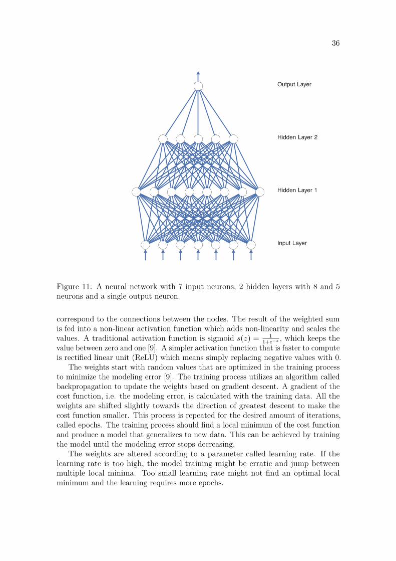
Nowadays, neural networks are one of the most popular machine learning methods.They mimic the working principle of the human brain in order to learn from a largeset of data. A simple neural network is the basis of neural network (NN) and deeplearning-based models. Such an architecture is presented in Figure 11. It consistsof multiple layers which have one or more neurons. All of the neurons are linkedwith weights that are presented by blue lines in Figure 11. The outputs from eachof the layers are used as inputs for the next layer until the last layer gives out thedesired output. The inputs and outputs of a single neuron are real numbers that getmultiplied by the weights connecting the neurons.

The first layer is the input layer which has as many neurons as there are inputvariables in the model. Figure 11 has 7 inputs which could be the last 7 observationsof a time series for example. The last layer of the neural network is always the outputof the model. The number of neurons in the last layer corresponds to the desiredamount of output variables. For example in Figure 11 the single output could be aprediction for the next value of the time series.

The layers between the input and output layers are called hidden layers. Thenumber of hidden layers and the number of neurons in them can be chosen arbitrarily.Neural networks which have more than one hidden layer are called deep neuralnetworks (DNN). More layers and neurons enable the model to learn more complexpatterns at the cost of increasing the training time and possibly causing overfitting.

Each node in the layer gets its inputs from the nodes of the previous layer.The input is the sum of the incoming connections multiplied by the weights that

36

Input Layer

Hidden Layer 1

Hidden Layer 2

Output Layer

Figure 11: A neural network with 7 input neurons, 2 hidden layers with 8 and 5neurons and a single output neuron.

correspond to the connections between the nodes. The result of the weighted sumis fed into a non-linear activation function which adds non-linearity and scales thevalues. A traditional activation function is sigmoid s(z) = 1

1+e−z , which keeps thevalue between zero and one [9]. A simpler activation function that is faster to computeis rectified linear unit (ReLU) which means simply replacing negative values with 0.

The weights start with random values that are optimized in the training processto minimize the modeling error [9]. The training process utilizes an algorithm calledbackpropagation to update the weights based on gradient descent. A gradient of thecost function, i.e. the modeling error, is calculated with the training data. All theweights are shifted slightly towards the direction of greatest descent to make thecost function smaller. This process is repeated for the desired amount of iterations,called epochs. The training process should find a local minimum of the cost functionand produce a model that generalizes to new data. This can be achieved by trainingthe model until the modeling error stops decreasing.

The weights are altered according to a parameter called learning rate. If thelearning rate is too high, the model training might be erratic and jump betweenmultiple local minima. Too small learning rate might not find an optimal localminimum and the learning requires more epochs.

37

2.9.2 RNN

The simple neural network architecture that was presented in the previous sectioncan work with very short and simple time series. Feeding lagged values of the timeseries to the input neurons of the neural network enables the model to learn simpletime dependence of the observations. However, the model has no memory of the pasttime steps which means that it does not know anything about the time series fromlags higher than the number of input neurons.

Recurrent neural networks (RNN) were developed to enable the modeling oflonger sequential data like time series [27]. They are very similar to the architecturepresented earlier, but the input of each neuron consists of a sum of the current inputand the output of the neural network from the previous time step. The outputfrom the previous time step contains the outputs of all the previous time steps dueto the recursive nature of the learning process. This means that the model has amemory of the whole dataset. However, the effect of past observations starts todecay quite quickly and the effective memory depth of one RNN neuron is about 10time steps [34]. The next Section 2.9.3 presents LSTM neural networks which havea significantly better memory compared to RNNs.

Each neuron in the RNN has two sets of weights, one for the current input valueand another for the output of the previous time step. The weights are learnedsimilar to normal neural networks, but the recursive nature of the model needs to beunrolled through time. The weights are adjusted starting from the latest time steppropagating backwards towards the first time step. Like regular neural networks,also RNNs can contain multiple layers and an arbitrary number of neurons per layer.If the time series contains seasonality, it is beneficial to also include inputs from theprevious season.

2.9.3 Long short-term memory (LSTM)

Long short-term memory (LSTM) neural networks are an adaptation of RNNs thatcan be used to model longer sequences. They were first proposed in [37] and theyhave since been further improved. RNNs with long-term memory have proven souseful that regular RNNs are rarely used anymore [34].

The main idea behind LSTM neurons is that they have a long-term and a short-term state. At every time step, some of the unnecessary information is forgottenin the long-term state and some new information is learned. The short-term stateis produced with the long-term state and it represents the modeled value for thecurrent time step.

Implementation details of RNN and LSTM models are out-of-scope of this thesis,but most machine learning frameworks like keras [38] have implemented LSTMneurons which makes them easy to use.

2.9.4 Decision tree models

Decision tree-based methods are commonly used machine learning algorithms inreal-world applications [27]. They are flexible, fast and easy to interpret which makes

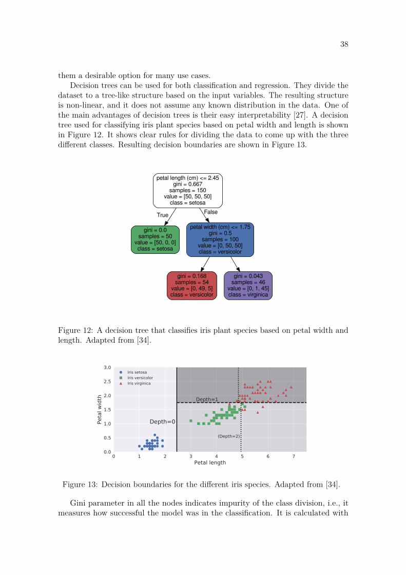
38

them a desirable option for many use cases.Decision trees can be used for both classification and regression. They divide the

dataset to a tree-like structure based on the input variables. The resulting structureis non-linear, and it does not assume any known distribution in the data. One ofthe main advantages of decision trees is their easy interpretability [27]. A decisiontree used for classifying iris plant species based on petal width and length is shownin Figure 12. It shows clear rules for dividing the data to come up with the threedifferent classes. Resulting decision boundaries are shown in Figure 13.

petal length (cm) <= 2.45gini = 0.667

samples = 150value = [50, 50, 50]

class = setosa

gini = 0.0samples = 50

value = [50, 0, 0]class = setosa

True

petal width (cm) <= 1.75gini = 0.5

samples = 100value = [0, 50, 50]class = versicolor

False

gini = 0.168samples = 54

value = [0, 49, 5]class = versicolor

gini = 0.043samples = 46

value = [0, 1, 45]class = virginica

Figure 12: A decision tree that classifies iris plant species based on petal width andlength. Adapted from [34].

0 1 2 3 4 5 6 7Petal length

0.0

0.5

1.0

1.5

2.0

2.5

3.0

Peta

l wid

th

Depth=0

Depth=1

(Depth=2)

Iris setosaIris versicolorIris virginica

Figure 13: Decision boundaries for the different iris species. Adapted from [34].

Gini parameter in all the nodes indicates impurity of the class division, i.e., itmeasures how successful the model was in the classification. It is calculated with

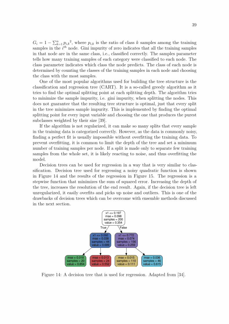
39

Gi = 1 − ∑nk=1 pi,k

2, where pi,k is the ratio of class k samples among the trainingsamples in the ith node. Gini impurity of zero indicates that all the training samplesin that node are in the same class, i.e., classified correctly. The samples parametertells how many training samples of each category were classified to each node. Theclass parameter indicates which class the node predicts. The class of each node isdetermined by counting the classes of the training samples in each node and choosingthe class with the most samples.

One of the most popular algorithms used for building the tree structure is theclassification and regression tree (CART). It is a so-called greedy algorithm as ittries to find the optimal splitting point at each splitting depth. The algorithm triesto minimize the sample impurity, i.e. gini impurity, when splitting the nodes. Thisdoes not guarantee that the resulting tree structure is optimal, just that every splitin the tree minimizes sample impurity. This is implemented by finding the optimalsplitting point for every input variable and choosing the one that produces the purestsubclasses weighted by their size [39].

If the algorithm is not regularized, it can make so many splits that every samplein the training data is categorized correctly. However, as the data is commonly noisy,finding a perfect fit is usually impossible without overfitting the training data. Toprevent overfitting, it is common to limit the depth of the tree and set a minimumnumber of training samples per node. If a split is made only to separate few trainingsamples from the whole set, it is likely reacting to noise, and thus overfitting themodel.

Decision trees can be used for regression in a way that is very similar to clas-sification. Decision tree used for regressing a noisy quadratic function is shownin Figure 14 and the results of the regression in Figure 15. The regression is astepwise function that minimizes the sum of squared error. Increasing the depth ofthe tree, increases the resolution of the end result. Again, if the decision tree is leftunregularized, it easily overfits and picks up noise and outliers. This is one of thedrawbacks of decision trees which can be overcome with ensemble methods discussedin the next section.

x1 <= 0.197mse = 0.098

samples = 200value = 0.354

x1 <= 0.092mse = 0.038samples = 44value = 0.689

True

x1 <= 0.772mse = 0.074

samples = 156value = 0.259

False

mse = 0.018samples = 20value = 0.854

mse = 0.013samples = 24value = 0.552

mse = 0.015samples = 110value = 0.111

mse = 0.036samples = 46value = 0.615

Figure 14: A decision tree that is used for regression. Adapted from [34].

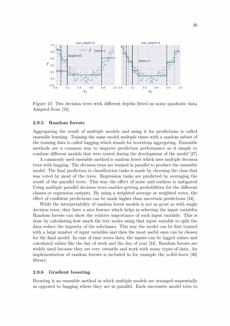
40

0.0 0.2 0.4 0.6 0.8 1.0x1

0.2

0.0

0.2

0.4

0.6

0.8

1.0

y

Depth=0

Depth=1

Depth=1

max_depth=2

y

0.0 0.2 0.4 0.6 0.8 1.0x1

Depth=2

max_depth=3

Figure 15: Two decision trees with different depths fitted on noisy quadratic data.Adapted from [34].

2.9.5 Random forests

Aggregating the result of multiple models and using it for predictions is calledensemble learning. Training the same model multiple times with a random subset ofthe training data is called bagging which stands for bootstrap aggregating. Ensemblemethods are a common way to improve prediction performance as it simple tocombine different models that were tested during the development of the model [27].

A commonly used ensemble method is random forest which uses multiple decisiontrees with bagging. The decision trees are trained in parallel to produce the ensemblemodel. The final prediction in classification tasks is made by choosing the class thatwas voted by most of the trees. Regression tasks are predicted by averaging theresult of the parallel trees. This way the effect of noise and outliers is mitigated.Using multiple parallel decision trees enables getting probabilities for the differentclasses or regression outputs. By using a weighted average or weighted votes, theeffect of confident predictions can be made higher than uncertain predictions [34].

While the interpretability of random forest models is not as great as with singledecision trees, they have a nice feature which helps in selecting the input variables.Random forests can show the relative importance of each input variable. This isdone by calculating how much the tree nodes using that input variable to split thedata reduce the impurity of the subclasses. This way the model can be first trainedwith a large number of input variables and then the most useful ones can be chosenfor the final model. In case of time series data, the inputs can be lagged values andcalculated values like the day of week and the day of year [34]. Random forests arewidely used because they are very versatile and work with many types of data. Animplementation of random forests is included in for example the scikit-learn [40]library.

2.9.6 Gradient boosting

Boosting is an ensemble method in which multiple models are arranged sequentiallyas opposed to bagging where they are in parallel. Each successive model tries to

41

correct the errors of their predecessor. The later models in the sequence focus onlyon the parts of the data that the earlier models failed to model.

Overfitting is a concern with this method, so regularization is required. Onesuitable method is to keep track of the modeling error as more models are added tothe sequence. If the modeling error stops decreasing significantly, the training shouldbe stopped. This is called early stopping [27].

A widely used modeling technique called gradient boosting was first introducedin [41] and further improved in [42]. It uses sequential decision trees that correct theresidual errors of the previous trees. Early stopping and adjusting the weight of eachsequential decision tree are valid methods for regularizing gradient boosting models.

Gradient boosting is implemented in the scikit-learn [40] python library. A moreadvanced version called Extreme Gradient Boosting is implemented in a pythonlibrary called XGBoost [43]. It has a similar API to scikit-learn but it has beenoptimized to be faster and more scalable. It includes an automatic implementationof early stopping which makes it simple to use.

2.10 ForecastingForecasting is one of the most useful use cases for time series models. It can giveinsight into the future of processes and systems which can be invaluable when makingdecisions. The following sections focus on how to produce forecasts with time seriesmodels and how to validate their performance.

2.10.1 Producing forecasts with a model

Producing forecasts with a model is usually done one time step at a time dependingon the model. For simple models, the prediction for the next observation is predictedby simply feeding the model with the past observations and setting the error term εt

to zero as the random error cannot be predicted in advance. If a long-term forecastis required, the predictions are added to the end of the observed data and the modelis applied again. As the forecast horizon, i.e. the number of time steps predicted getslarger, the uncertainty of the forecast increases. This is caused by the modeling erroradding up when the predicted values from earlier time steps are added as inputsto the time series model. Stochastic models can predict probability distributionsfor future time steps using the past observations as input. Expected value of thepredicted distribution is the point forecast and the error can be derived from thedistribution. Some models utilize information that is known in advance, e.g. holidaysand the days of week, which can be calculated using a calendar [9].

The uncertainty of the forecast is almost as important as the forecast itself. With-out knowing the prediction intervals, the value of the forecast is limited. Predictionintervals can be directly calculated for some of the simpler linear stochastic models.However, more complex models cannot output any statistical measure of their cer-tainty. In such cases bagging is a useful tool. By making hundreds of forecasts withrandom subsets of the data, the distribution can be estimated [9].

42

2.10.2 Evaluating forecast accuracy

An important measure of performance is to calculate the forecasting error with a testset of data. The test set is usually taken from the end of the dataset before fitting themodel. Making predictions on the test set simulates forecasting in real productionenvironment where the future values are unknown. Comparing the forecast with theactual observations, a clear picture of the performance of the model can be seen [27].

Different error metrics are used for comparing the forecasted values and actualobservations. There is no one perfect error measure that can be used as is. Differenterror metrics reveal different things about the model performance. To get a goodunderstanding, multiple error metrics need to be calculated and compared critically.Some error metrics suitable for evaluating point forecasts are listed below.

Error metrics that measure absolute error penalize both positive and negativeerrors, but they do not reveal if the model predicts too high or low on average. Meanerrors show bias, but positive and negative errors cancel each other out. Percentageerrors are scale independent which is helpful for data that has a trend or largefluctuations in level. This way the error metric does not bias the parts of datawith higher level [9]. Some of the most common error metrics are presented in thefollowing list:

Root mean squared error (RMSE) is defined as:

RMSE =

⌜⎷ 1T

T∑t=1

(yt − yt)2,

where yt is the predicted value, yt the observed value and T the length of the timeseries. It has the same scale as the data and positive and negative errors do not canceleach other out. These properties make RMSE a good starting point for evaluatingthe magnitude of forecasting errors. Sometime RMSE is normalized by dividing it bythe mean value of the observations y. This indicates the scale of the error in relationto the scale of the time series. This makes it easier to compare the performancebetween datasets with different scales.

Mean absolute percentage error (MAPE) is defined as:

MAPE = 1T

T∑t=1

(100

yt − yt

yt

)

.

MAPE is scale independent, as every error is divided by yt. This is useful as it tiesthe magnitude of the errors to the overall level of the time series. However, if thetime series goes near zero, the relative error might become very large and unstable.As the absolute values of the relative errors are averaged, positive and negative errorsdo not cancel out.

Mean bias error (MBE) is defined as:

MBE = 1T

T∑t=1

(yt − yt) .

43

It shows if the forecasted values have bias, i.e., they are on average too high ortoo low. As positive and negative errors cancel each other out, MBE is not usefulfor estimating the magnitude of the error. However, having significant bias in theforecasts will cause systematic errors in the forecasts. This makes MBE an importantmetric.

Akaike information criterion (AIC) is defined as:AIC = −2 log(L) + 2k,

where L is the likelihood of the data and k is the number of parameters in the model.k includes σ2, i.e., the variance of the residuals as an estimable parameter. AIC errorpenalizes models with a large number of parameters because they are likely to causeoverfitting. Choosing the model with the lowest AIC will probably work the bestwith out-of-sample predictions [9].

Schwarz’s Bayesian Information Criterion (BIC) is defined as:BIC = −2 log(L) + k log(T ).

It is similar to AIC but it favors even less model parameters. Choosing a modelbased on BIC is either the same model as would be chosen by AIC or a model withfewer parameters [9].

Prediction intervals can be quite simply evaluated for forecasting methods thatproduce them. If 95 % prediction intervals are calculated for step-ahead forecasts,approximately 95 % of the observed values should be inside the prediction intervals.More formal statistical tests exist for measuring the forecasting performance ofstochastic models, but they are not used in this thesis. A commonly used metric islogarithmic scoring rule [44].

When comparing multiple models, it should be relatively simple to choose thebest-performing one based on the above error metrics. However, it is important tokeep in mind that the error metrics themselves could favor some models more thanothers. The achievable accuracy is largely dependent on the data which means thatthe performance is difficult to judge just with the calculated error metrics. To get anunderstanding of the performance, the models can be compared against a benchmark.A simple benchmark is a so-called naïve model. It predicts all future values as thelast known value. For seasonal time series the corresponding value from the lastavailable season is used as the prediction. If the more complicated model does notoutperform the naïve model, it probably is not working adequately.

Cross-validation is a good method for estimating forecasting error for forecasthorizons significantly shorter than the test set. An illustration of cross-validationis shown in Figure 16. The error calculation advances one time step at a time andthe errors are averaged from every time step. The first forecast horizon of data ispredicted using the training data. Then the forecast error from the first predictions iscalculated. Then the same process is repeated one time step further so that the firstvalue of the test set is added to the training set and the forecast horizon is shiftedby one. Averaging the errors for each time step tested gives a reliable estimate of theperformance of the model.

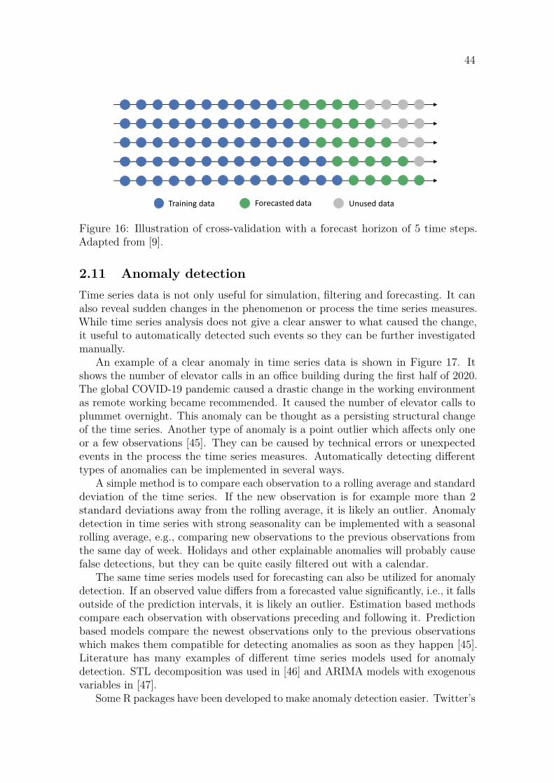
44

Training data Forecasted data Unused data

Figure 16: Illustration of cross-validation with a forecast horizon of 5 time steps.Adapted from [9].

2.11 Anomaly detectionTime series data is not only useful for simulation, filtering and forecasting. It canalso reveal sudden changes in the phenomenon or process the time series measures.While time series analysis does not give a clear answer to what caused the change,it useful to automatically detected such events so they can be further investigatedmanually.

An example of a clear anomaly in time series data is shown in Figure 17. Itshows the number of elevator calls in an office building during the first half of 2020.The global COVID-19 pandemic caused a drastic change in the working environmentas remote working became recommended. It caused the number of elevator calls toplummet overnight. This anomaly can be thought as a persisting structural changeof the time series. Another type of anomaly is a point outlier which affects only oneor a few observations [45]. They can be caused by technical errors or unexpectedevents in the process the time series measures. Automatically detecting differenttypes of anomalies can be implemented in several ways.

A simple method is to compare each observation to a rolling average and standarddeviation of the time series. If the new observation is for example more than 2standard deviations away from the rolling average, it is likely an outlier. Anomalydetection in time series with strong seasonality can be implemented with a seasonalrolling average, e.g., comparing new observations to the previous observations fromthe same day of week. Holidays and other explainable anomalies will probably causefalse detections, but they can be quite easily filtered out with a calendar.

The same time series models used for forecasting can also be utilized for anomalydetection. If an observed value differs from a forecasted value significantly, i.e., it fallsoutside of the prediction intervals, it is likely an outlier. Estimation based methodscompare each observation with observations preceding and following it. Predictionbased models compare the newest observations only to the previous observationswhich makes them compatible for detecting anomalies as soon as they happen [45].Literature has many examples of different time series models used for anomalydetection. STL decomposition was used in [46] and ARIMA models with exogenousvariables in [47].

Some R packages have been developed to make anomaly detection easier. Twitter’s

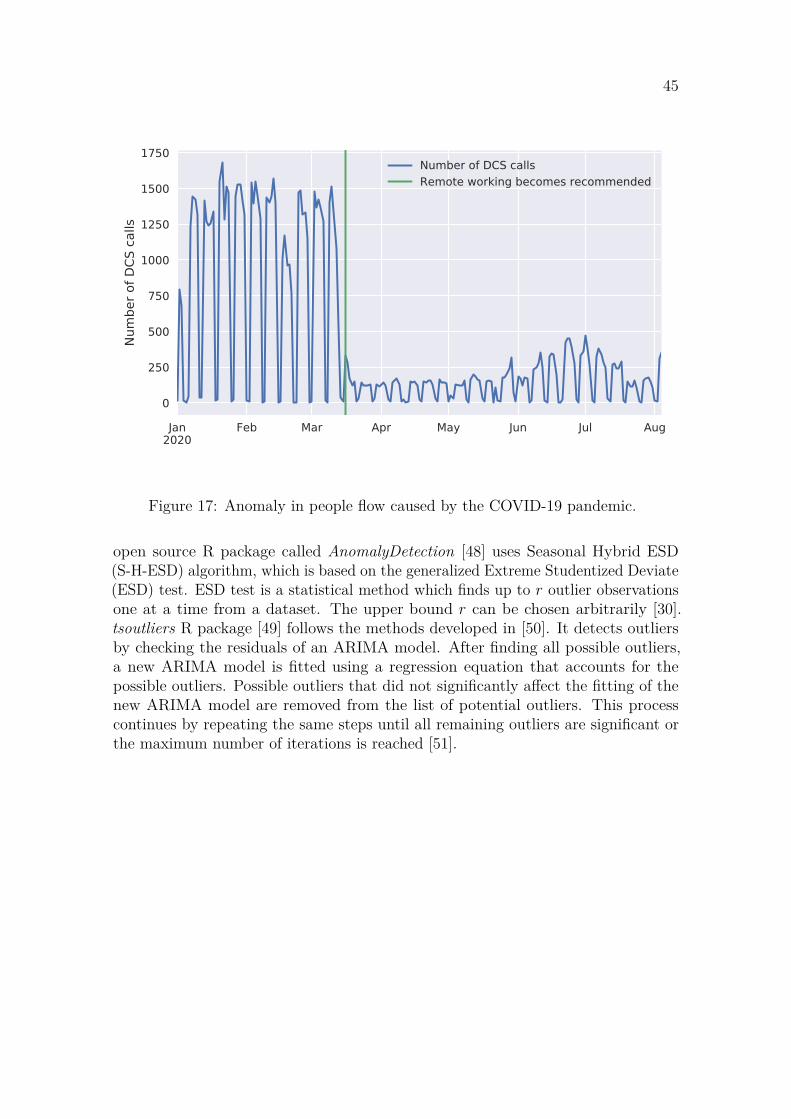
45

Jan2020

Feb Mar Apr May Jun Jul Aug

0

250

500

750

1000

1250

1500

1750

Num

ber o

f DCS

cal

ls

Number of DCS callsRemote working becomes recommended

Figure 17: Anomaly in people flow caused by the COVID-19 pandemic.

open source R package called AnomalyDetection [48] uses Seasonal Hybrid ESD(S-H-ESD) algorithm, which is based on the generalized Extreme Studentized Deviate(ESD) test. ESD test is a statistical method which finds up to r outlier observationsone at a time from a dataset. The upper bound r can be chosen arbitrarily [30].tsoutliers R package [49] follows the methods developed in [50]. It detects outliersby checking the residuals of an ARIMA model. After finding all possible outliers,a new ARIMA model is fitted using a regression equation that accounts for thepossible outliers. Possible outliers that did not significantly affect the fitting of thenew ARIMA model are removed from the list of potential outliers. This processcontinues by repeating the same steps until all remaining outliers are significant orthe maximum number of iterations is reached [51].

46

3 Materials and methodsElevator-specific terms and statistics used in this thesis are defined in Section 3.1.Datasets used for the time series modeling are presented and explored in Section 3.2.Section 3.3 outlines implications for modeling based on the data exploration. Morethorough descriptions of the modeling and experimentation methods are in Sec-tions 3.4-3.7.

3.1 Elevator-specific terms and statisticsDifferent elevator-specific terms and statistics are used for evaluating elevator trafficperformance. The terms and metrics used in this thesis are described in the followinglist:

Landing call is an elevator call made with conventional up and down buttons in anelevator lobby [52].

DCS call is an elevator call made with destination control system (DCS). Witha DCS system, the user selects the destination floor using a destination operatingpanel (DOP) when they make the call in the elevator lobby [52].

Call time (CT) indicates the time from a landing call to the arrival of an elevatorto the elevator lobby where the call was made from. The elevator is considered toarrive when it starts to decelerate before stopping.

Waiting time (WT) indicates the time from when a passenger either registers aDCS call, or joins a queue, until the responding elevator begins to open its doors atthe boarding floor [53].

Time to destination (TTD) indicates the time from when a passenger eitherregisters a DCS call, or joins a queue, until the responding elevator begins to openits doors at the destination floor [53].

3.2 DataThe main dataset for the experiments was collected from a Finnish office building.The elevator system in the building is a so-called hybrid system where the entrancefloors use a destination control system (DCS) and the upper floors have conventionalup and down landing call buttons.

The data was acquired from an elevator monitoring system database which collectsdata from the elevator group. The database contains dozens of different metrics, butthe following were chosen as variables of interest for the time series modeling:

• Number of landing calls per day

• Daily average landing call time

• Daily maximum 15-minute average landing call time

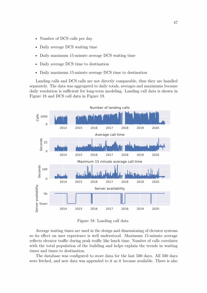
47

• Number of DCS calls per day

• Daily average DCS waiting time

• Daily maximum 15-minute average DCS waiting time

• Daily average DCS time to destination

• Daily maximum 15-minute average DCS time to destination

Landing calls and DCS calls are not directly comparable, thus they are handledseparately. The data was aggregated to daily totals, averages and maximums becausedaily resolution is sufficient for long-term modeling. Landing call data is shown inFigure 18 and DCS call data in Figure 19.

2014 2015 2016 2017 2018 2019 20200

1000

Calls

Number of landing calls

2014 2015 2016 2017 2018 2019 20200

25

Seco

nds

Average call time

2014 2015 2016 2017 2018 2019 20200

100

Seco

nds

Maximum 15 minute average call time

2014 2015 2016 2017 2018 2019 2020Down

Up

Serv

er a

vaila

bilit

y

Server availability

Figure 18: Landing call data

Average waiting times are used in the design and dimensioning of elevator systemsso its effect on user experience is well understood. Maximum 15-minute averagereflects elevator traffic during peak traffic like lunch time. Number of calls correlateswith the total population of the building and helps explain the trends in waitingtimes and times to destination.

The database was configured to store data for the last 500 days. All 500 dayswere fetched, and new data was appended to it as it became available. There is also

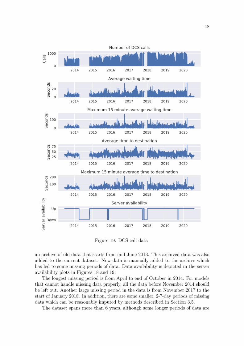
48

2014 2015 2016 2017 2018 2019 20200

1000

Calls

Number of DCS calls

2014 2015 2016 2017 2018 2019 20200

20

Seco

nds

Average waiting time

2014 2015 2016 2017 2018 2019 20200

100

Seco

nds

Maximum 15 minute average waiting time

2014 2015 2016 2017 2018 2019 2020255075

Seco

nds

Average time to destination

2014 2015 2016 2017 2018 2019 2020

100

200

Seco

nds

Maximum 15 minute average time to destination

2014 2015 2016 2017 2018 2019 2020Down

Up

Serv

er a

vaila

bilit

y

Server availability

Figure 19: DCS call data

an archive of old data that starts from mid-June 2013. This archived data was alsoadded to the current dataset. New data is manually added to the archive whichhas led to some missing periods of data. Data availability is depicted in the serveravailability plots in Figures 18 and 19.

The longest missing period is from April to end of October in 2014. For modelsthat cannot handle missing data properly, all the data before November 2014 shouldbe left out. Another large missing period in the data is from November 2017 to thestart of January 2018. In addition, there are some smaller, 2-7-day periods of missingdata which can be reasonably imputed by methods described in Section 3.5.

The dataset spans more than 6 years, although some longer periods of data are

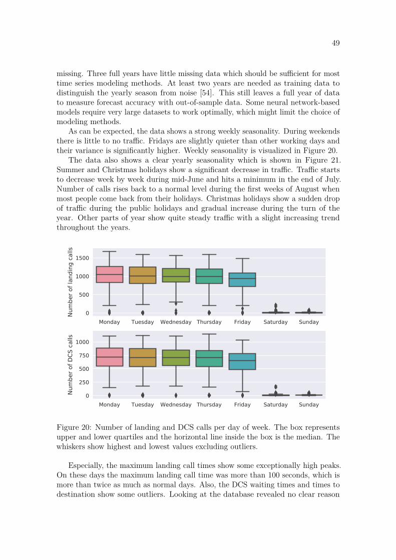
49

missing. Three full years have little missing data which should be sufficient for mosttime series modeling methods. At least two years are needed as training data todistinguish the yearly season from noise [54]. This still leaves a full year of datato measure forecast accuracy with out-of-sample data. Some neural network-basedmodels require very large datasets to work optimally, which might limit the choice ofmodeling methods.

As can be expected, the data shows a strong weekly seasonality. During weekendsthere is little to no traffic. Fridays are slightly quieter than other working days andtheir variance is significantly higher. Weekly seasonality is visualized in Figure 20.

The data also shows a clear yearly seasonality which is shown in Figure 21.Summer and Christmas holidays show a significant decrease in traffic. Traffic startsto decrease week by week during mid-June and hits a minimum in the end of July.Number of calls rises back to a normal level during the first weeks of August whenmost people come back from their holidays. Christmas holidays show a sudden dropof traffic during the public holidays and gradual increase during the turn of theyear. Other parts of year show quite steady traffic with a slight increasing trendthroughout the years.

Monday Tuesday Wednesday Thursday Friday Saturday Sunday0

500

1000

1500

Num

ber o

f lan

ding

cal

ls

Monday Tuesday Wednesday Thursday Friday Saturday Sunday0

250

500

750

1000

Num

ber o

f DCS

cal

ls

Figure 20: Number of landing and DCS calls per day of week. The box representsupper and lower quartiles and the horizontal line inside the box is the median. Thewhiskers show highest and lowest values excluding outliers.

Especially, the maximum landing call times show some exceptionally high peaks.On these days the maximum landing call time was more than 100 seconds, which ismore than twice as much as normal days. Also, the DCS waiting times and times todestination show some outliers. Looking at the database revealed no clear reason

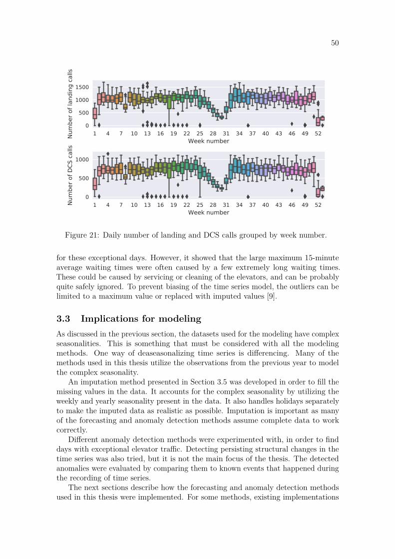
50

1 4 7 10 13 16 19 22 25 28 31 34 37 40 43 46 49 52Week number

0

500

1000

1500

Num

ber o

f lan

ding

cal

ls

1 4 7 10 13 16 19 22 25 28 31 34 37 40 43 46 49 52Week number

0

500

1000

Num

ber o

f DCS

cal

ls

Figure 21: Daily number of landing and DCS calls grouped by week number.

for these exceptional days. However, it showed that the large maximum 15-minuteaverage waiting times were often caused by a few extremely long waiting times.These could be caused by servicing or cleaning of the elevators, and can be probablyquite safely ignored. To prevent biasing of the time series model, the outliers can belimited to a maximum value or replaced with imputed values [9].

3.3 Implications for modelingAs discussed in the previous section, the datasets used for the modeling have complexseasonalities. This is something that must be considered with all the modelingmethods. One way of deaseasonalizing time series is differencing. Many of themethods used in this thesis utilize the observations from the previous year to modelthe complex seasonality.

An imputation method presented in Section 3.5 was developed in order to fill themissing values in the data. It accounts for the complex seasonality by utilizing theweekly and yearly seasonality present in the data. It also handles holidays separatelyto make the imputed data as realistic as possible. Imputation is important as manyof the forecasting and anomaly detection methods assume complete data to workcorrectly.

Different anomaly detection methods were experimented with, in order to finddays with exceptional elevator traffic. Detecting persisting structural changes in thetime series was also tried, but it is not the main focus of the thesis. The detectedanomalies were evaluated by comparing them to known events that happened duringthe recording of time series.

The next sections describe how the forecasting and anomaly detection methodsused in this thesis were implemented. For some methods, existing implementations

51

found in different software packages are used. Other methods were developed in thisthesis and they are described in more thorough detail.

3.4 Smart seasonal differencing and smart lagThis section defines a so-called smart lag operator S(yt) which is utilized in theforecasting and anomaly detection methods described in the following sections. Thedatasets used in this thesis consists of daily observations that have strong yearly andweekly seasonality. To make the time series stationary, the seasonalities need to beremoved by decomposition or differencing. Simple seasonal differencing works withtime series that have only one seasonality of a constant period [9]. To handle boththe weekly and yearly seasonalities as well as the effect of holidays, smart seasonaldifferencing based on the so-called smart lag operator was developed in this thesis.

The smart lag operator S(yt) gives the value yt−k from the previous year thatcorresponds to time t. It accounts for weekly seasonality by selecting an observationfrom the same day of week. Yearly seasonality is considered by using the observationfrom the same week of year. If the observation from the same week of year is missingor it is a holiday, the observation is chosen from the previous or following weeks ofyear. Observations are searched up to 3 weeks preceding and following the week thatcorresponds to the current observation. First the previous week is checked, then thefollowing week and so on. If a suitable observation is not found within ±3 weeks,smart lag returns a missing value. If yt is an observation from a holiday, S(yt) ischosen by selecting the same holiday’s observation from the previous year using acalendar. If yt is not a holiday, it is also ensured using the ±3 week tolerance thatS(yt) is not an observation from a holiday. Using these rules to select k also handlesleap years without problems. In order to mitigate outliers, the value of the smart lagis clipped to 90 % quantile of the whole time series. This is done to ensure that thesmart lag returned is a sensible presentation of the whole time series.

Smart seasonal differenced time series is defined as y′t = yt −S(yt). Smart seasonal

differencing is inverted by adding the value from the previous year based on thesame rules, i.e., yt = y′

t + S(yt). However, the differencing loses the first year ofdata as the values from the year before it are not available. This means the inverseoperation needs to be given the first year of the undifferenced data which is addedto the first year of differenced data to get back the original values. If a forecast ismade using smart seasonally differenced data, it can be inverse differenced using thesame method.

3.5 Imputing missing values in dataThe datasets in this thesis contain some periods of missing data as was discussed inSection 3.2. While this situation is not ideal, it is quite typical. To use methods thatrequire complete data, the missing values need to be imputed based on the availabledata. However, it is important to keep in mind that imputing does not add any newinformation to the dataset.

52

Distinguishing between days whose data is missing and days that had no trafficis required so valid days are not filled with imputed data. Using the database, dayswith partially or completely missing data were marked as invalid. This ensures thatsmall gaps in the data during the day will not skew the daily totals, averages andmaximums.

Missing values can be imputed in several ways. The data has high yearly andweekly seasonality as shown in Section 3.2. It means that the simplest methods likecarrying over the last known value or filling missing values with the mean of thedata are not suitable. However, similar approaches can be adapted to account forthe seasonality to make them work. Three such methods are compared in this thesis.One of them is na_seasplit() function from imputeTS R package [24]. It has someshortcomings with default settings which are corrected in the second method whichis based on na_seasplit(). The third method is developed in this thesis with theobservations made from the first two methods and it provided the basis for the smartlag operator defined earlier.

na_seasplit() splits the data to year-long periods. It uses linear interpolationby default to impute values. The imputed value is the average of the same dayfrom the preceding and following year. If the value for previous or next year isnot available, last observation carried forward (LOCF) or next observation carriedbackward (NOCB) is used instead. If values from both the previous and followingyear are unavailable, the missing value is not imputed. na_seasplit() matches thedays from different years based on the number of days from the beginning of theyear. This causes problems as the average is calculated from different days of week.If LOCF is used instead of interpolation, the imputed values are still from a wrongday of week. This issue is caused by the length of the weekly seasonality not being amultiple of the yearly season. Handling complex seasonality is widely covered topicin literature, e.g. De Livera et al. [33].

There are 52 weeks in a year and 7 days in a week. However, 7 × 52 = 364 doesnot add up to 365 days in a year. This means that the weekly seasonality shifts byone day in a regular year and two days in a leap year. For example the 100th dayin 2012 was a Monday. If its value was to be filled with the value of the 100th dayof 2011, it would be severely underestimated as that day was a Sunday. This canbe corrected by imputing the value with the 101st day of 2011 but then holidayswould be misaligned by one day. Leap days complicate the issue even more as theday offset increases by one after the leap day. Public holidays with different datesyear-to-year like Easter make the seasonality adjustment even more difficult.

To correct the above issue, LOCF was chosen as the algorithm for na_seasplit() inthe second method. Imputed values were shifted backwards by one day to make theweekly seasonality correct. Holidays were handled with a country-specific calendarin the fbprophet library [55]. Because the amount of traffic on a holiday does notpresumably depend on the week of day, the one-day shift was not used for them andunshifted values were used instead. The value for each day preceding a holiday isthe same as the value of the holiday because of the one-day shift. To correct this,days preceding holidays were filled with the average of the same day of week fromthe preceding and following weeks. This way the holidays were put back to correct

53

dates and the days preceding holidays were imputed as regular days. This works wellfor holidays that happen on the same date every year but holidays like Easter arestill problematic.

The third method, called seasonal method, tries to combine the best aspects ofthe first two methods and overcome their problems. Linear interpolation is betterthan LOCF, as it can account for a trend in the data. Handling holidays with acalendar is a good idea but it should also work with Easter. This is achieved byutilizing the smart lag operator S(yt) defined in Section 3.4.

In order to use linear interpolation to impute missing values, in addition tothe value from the previous year, also the value from the following year is needed.Following year’s value is acquired with a smart lead operator L(yt) = yt+k, whichfollows a similar logic as the smart lag operator S(yt). If the corresponding values forboth the preceding and following years are available, the imputed value is calculatedas their average. If only one of the values is available, the imputed value is that value,i.e., LOCF or NOCB is used. If both smart lag and smart lead are not available, thevalue is left temporarily unimputed. After the smart lag and lead based imputation,any missing values are imputed with a rolling mean of the same days of week tomake sure there are no missing values left after the imputation.

All three methods were compared by first filling in the DCS call dataset with theseasonal method to mitigate the bias of missing data. Then three months of existingdata was removed from the filled test dataset. The data was deleted from June 2017to the end of August 2017. This period was chosen, as imputing the values for thesummer holiday period tests the ability to account for yearly seasonality. Year 2017was chosen because its data is not actually missing and there is a large increase inthe number of calls from 2016 to 2017. The increase in traffic tests the ability toaccount for a trend in the data. DCS call dataset was chosen as it contains times todestination in addition to waiting times and number of calls. Times to destinationdiffer from the other data columns as they can never be zero.

All three methods were used to fill the deleted period of data. Imputation errorwas calculated for all three methods by comparing the imputed values with the actualvalues. Root mean square (RMS) errors for all three of the methods are summarizedin Table 2. Comparison of the seasonal method and default na_seasplit() is shown inFigure 22. Seasonal method is compared against the corrected na_seasplit() methodin Figure 23.

na_seasplit() with default parameters performed very poorly. Imputed values forthe weekends were significantly higher than the actual values. This is caused by thelinear interpolation and offset in the weekly seasonality. Because 2016 was a leapyear, values for Sundays are imputed as the average of a Friday from last year and aMonday from the following year. Misaligned weekly seasonality shows as large spikesin the error plot in Figure 22.

The corrected na_seasplit() method performs very similarly to the seasonalmethod. However, it clearly predicts too low values for the number of calls as can beseen in Figure 23. This is caused by the LOCF algorithm that does not account forthe trend in the data. In times to destination the corrected na_seaplit() performseven slightly better than the seasonal method based on the RMS error.

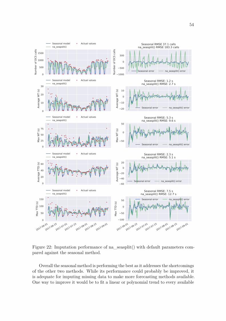
54

0

500

1000

1500

Num

ber o

f DCS

cal

ls

Seasonal modelna_seapslit()

Actual values

1000

500

0

500

Num

ber o

f DCS

cal

ls

Seasonal RMSE 37.1 callsna_seasplit() RMSE 183.3 calls

Seasonal error na_seasplit() error

0

10

20

30

Aver

age

WT

(s)

Seasonal modelna_seapslit()

Actual values

20

10

0

10

Aver

age

WT

(s)

Seasonal RMSE: 1.2 sna_seasplit() RMSE: 2.7 s

Seasonal error na_seasplit() error

0

25

50

75

Max

WT

(s)

Seasonal modelna_seapslit()

Actual values

50

0

50

Max

WT

(s)

Seasonal RMSE: 5.3 sna_seasplit() RMSE: 9.6 s

Seasonal error na_seasplit() error

0

20

40

60

Aver

age

TTD

(s)

Seasonal modelna_seapslit()

Actual values

60

40

20

0

20

Aver

age

WT

(s)

Seasonal RMSE: 2.3 sna_seasplit() RMSE: 5.1 s

Seasonal error na_seasplit() error

2017-06-01

2017-06-15

2017-07-01

2017-07-15

2017-08-01

2017-08-15

2017-09-010

50

100

150

Max

TTD

(s)

Seasonal modelna_seapslit()

Actual values

2017-06-01

2017-06-15

2017-07-01

2017-07-15

2017-08-01

2017-08-15

2017-09-01100

50

0

50

Max

TTD

(s)

Seasonal RMSE: 7.5 sna_seasplit() RMSE: 12.7 sSeasonal error na_seasplit() error

Figure 22: Imputation performance of na_seasplit() with default parameters com-pared against the seasonal method.

Overall the seasonal method is performing the best as it addresses the shortcomingsof the other two methods. While its performance could probably be improved, itis adequate for imputing missing data to make more forecasting methods available.One way to improve it would be to fit a linear or polynomial trend to every available

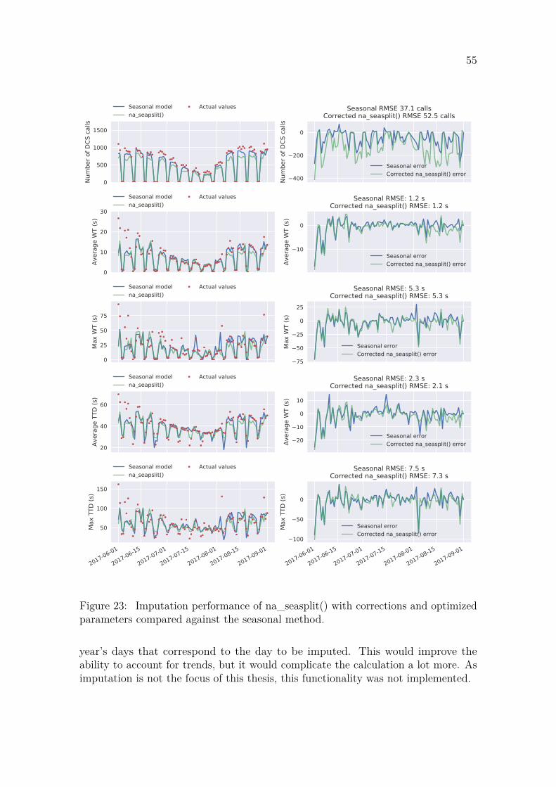
55

0

500

1000

1500

Num

ber o

f DCS

cal

ls

Seasonal modelna_seapslit()

Actual values

400

200

0

Num

ber o

f DCS

cal

ls

Seasonal RMSE 37.1 callsCorrected na_seasplit() RMSE 52.5 calls

Seasonal errorCorrected na_seasplit() error

0

10

20

30

Aver

age

WT

(s)

Seasonal modelna_seapslit()

Actual values

10

0

Aver

age

WT

(s)

Seasonal RMSE: 1.2 sCorrected na_seasplit() RMSE: 1.2 s

Seasonal errorCorrected na_seasplit() error

0

25

50

75

Max

WT

(s)

Seasonal modelna_seapslit()

Actual values

75

50

25

0

25

Max

WT

(s)

Seasonal RMSE: 5.3 sCorrected na_seasplit() RMSE: 5.3 s

Seasonal errorCorrected na_seasplit() error

20

40

60

Aver

age

TTD

(s)

Seasonal modelna_seapslit()

Actual values

20

10

0

10

Aver

age

WT

(s)

Seasonal RMSE: 2.3 sCorrected na_seasplit() RMSE: 2.1 s

Seasonal errorCorrected na_seasplit() error

2017-06-01

2017-06-15

2017-07-01

2017-07-15

2017-08-01

2017-08-15

2017-09-01

50

100

150

Max

TTD

(s)

Seasonal modelna_seapslit()

Actual values

2017-06-01

2017-06-15

2017-07-01

2017-07-15

2017-08-01

2017-08-15

2017-09-01100

50

0

Max

TTD

(s)

Seasonal RMSE: 7.5 sCorrected na_seasplit() RMSE: 7.3 s

Seasonal errorCorrected na_seasplit() error

Figure 23: Imputation performance of na_seasplit() with corrections and optimizedparameters compared against the seasonal method.

year’s days that correspond to the day to be imputed. This would improve theability to account for trends, but it would complicate the calculation a lot more. Asimputation is not the focus of this thesis, this functionality was not implemented.

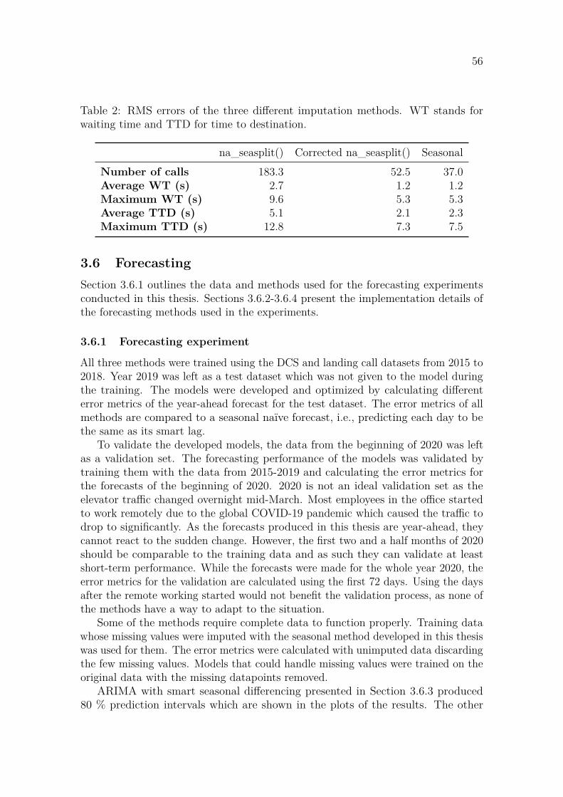
56

Table 2: RMS errors of the three different imputation methods. WT stands forwaiting time and TTD for time to destination.

na_seasplit() Corrected na_seasplit() SeasonalNumber of calls 183.3 52.5 37.0Average WT (s) 2.7 1.2 1.2Maximum WT (s) 9.6 5.3 5.3Average TTD (s) 5.1 2.1 2.3Maximum TTD (s) 12.8 7.3 7.5

3.6 ForecastingSection 3.6.1 outlines the data and methods used for the forecasting experimentsconducted in this thesis. Sections 3.6.2-3.6.4 present the implementation details ofthe forecasting methods used in the experiments.

3.6.1 Forecasting experiment

All three methods were trained using the DCS and landing call datasets from 2015 to2018. Year 2019 was left as a test dataset which was not given to the model duringthe training. The models were developed and optimized by calculating differenterror metrics of the year-ahead forecast for the test dataset. The error metrics of allmethods are compared to a seasonal naïve forecast, i.e., predicting each day to bethe same as its smart lag.

To validate the developed models, the data from the beginning of 2020 was leftas a validation set. The forecasting performance of the models was validated bytraining them with the data from 2015-2019 and calculating the error metrics forthe forecasts of the beginning of 2020. 2020 is not an ideal validation set as theelevator traffic changed overnight mid-March. Most employees in the office startedto work remotely due to the global COVID-19 pandemic which caused the traffic todrop to significantly. As the forecasts produced in this thesis are year-ahead, theycannot react to the sudden change. However, the first two and a half months of 2020should be comparable to the training data and as such they can validate at leastshort-term performance. While the forecasts were made for the whole year 2020, theerror metrics for the validation are calculated using the first 72 days. Using the daysafter the remote working started would not benefit the validation process, as none ofthe methods have a way to adapt to the situation.

Some of the methods require complete data to function properly. Training datawhose missing values were imputed with the seasonal method developed in this thesiswas used for them. The error metrics were calculated with unimputed data discardingthe few missing values. Models that could handle missing values were trained on theoriginal data with the missing datapoints removed.

ARIMA with smart seasonal differencing presented in Section 3.6.3 produced80 % prediction intervals which are shown in the plots of the results. The other

57

two methods do not support prediction intervals natively, which is why they arenot presented. Prediction intervals could be produced for all the methods with forexample bagging [9].

Error metrics chosen to measure forecasting performance are RMS error, bias (MBE)and normalized RMS error (NRMSE). Normalized RMS error was calculated bydividing the RMS error with the mean of the test dataset. It relates the magnitudeof the errors to the magnitude of the time series. It makes it easier to compare theperformance of the forecasts of different time series with different scales.

3.6.2 LSTM

keras [38] framework with Tensorflow [56] backend was used to implement the LSTMneural network model. The number of time steps used as input to the model andthe number of time steps forecasted at a time were experimented with during thedevelopment of the model. In the end, 120 time steps was found to be an appropriateinput. The model performed the best when it predicted one time step at a time, soone output was chosen. As neural networks can find complex dependencies amongmultiple variables, date features were added as input variables in addition to pastvalues. Date features consisted of the following:

• Boolean indicator is today a holiday

• Boolean indicator is tomorrow a holiday

• Day of week

• Day of month

• Day of year

• Week of year

• Year

LSTM neural networks remember the most prominent features of past time steps,but the depth of the memory is limited. In order to ensure the model knows whathappened one year ago, smart lag values of the input time steps were added asadditional variables. The date features and smart lag of the day to be forecasted arealso known before-hand, so they were added as additional columns to the input. Allthe input variables were scaled to a range between 0-1 to ensure they work correctlywith the activation functions used in the LSTM layers. The scaling was done usingRobustScaler from the scikit-learn [40] Python package to mitigate the effect ofoutlier values. Altogether the input data consisted of 120 × 17 values, where S(yt) isthe smart lag and D(yt) are the 7 date features for yt:

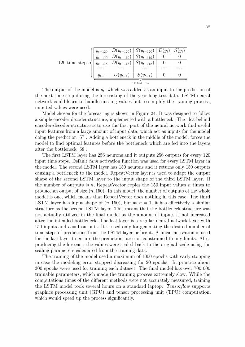
58

120 time-steps

⎧⎪⎪⎪⎪⎪⎪⎨⎪⎪⎪⎪⎪⎪⎩

yt−120 D(yt−120) S(yt−120) D(yt) S(yt)yt−119 D(yt−119) S(yt−119) 0 0yt−118 D(yt−118) S(yt−118) 0 0· · · · · · · · · · · · · · ·yt−1 D(yt−1) S(yt−1) 0 0⏞ ⏟⏟ ⏞

17 features

The output of the model is yt, which was added as an input to the prediction ofthe next time step during the forecasting of the year-long test data. LSTM neuralnetwork could learn to handle missing values but to simplify the training process,imputed values were used.

Model chosen for the forecasting is shown in Figure 24. It was designed to followa simple encoder-decoder structure, implemented with a bottleneck. The idea behindencoder-decoder structure is to use the first part of the neural network find usefulinput features from a large amount of input data, which act as inputs for the modeldoing the prediction [57]. Adding a bottleneck in the middle of the model, forces themodel to find optimal features before the bottleneck which are fed into the layersafter the bottleneck [58].

The first LSTM layer has 256 neurons and it outputs 256 outputs for every 120input time steps. Default tanh activation function was used for every LSTM layer inthe model. The second LSTM layer has 150 neurons and it returns only 150 outputscausing a bottleneck to the model. RepeatVector layer is used to adapt the outputshape of the second LSTM layer to the input shape of the third LSTM layer. Ifthe number of outputs is n, RepeatVector copies the 150 input values n times toproduce an output of size (n, 150). In this model, the number of outputs of the wholemodel is one, which means that RepeatVector does nothing in this case. The thirdLSTM layer has input shape of (n, 150), but as n = 1, it has effectively a similarstructure as the second LSTM layer. This means that the bottleneck structure wasnot actually utilized in the final model as the amount of inputs is not increasedafter the intended bottleneck. The last layer is a regular neural network layer with150 inputs and n = 1 outputs. It is used only for generating the desired number oftime steps of predictions from the LSTM layer before it. A linear activation is usedfor the last layer to ensure the predictions are not constrained to any limits. Afterproducing the forecast, the values were scaled back to the original scale using thescaling parameters calculated from the training data.

The training of the model used a maximum of 1000 epochs with early stoppingin case the modeling error stopped decreasing for 20 epochs. In practice about300 epochs were used for training each dataset. The final model has over 700 000trainable parameters, which made the training process extremely slow. While thecomputations times of the different methods were not accurately measured, trainingthe LSTM model took several hours on a standard laptop. Tensorflow supportsgraphics processing unit (GPU) and tensor processing unit (TPU) computation,which would speed up the process significantly.

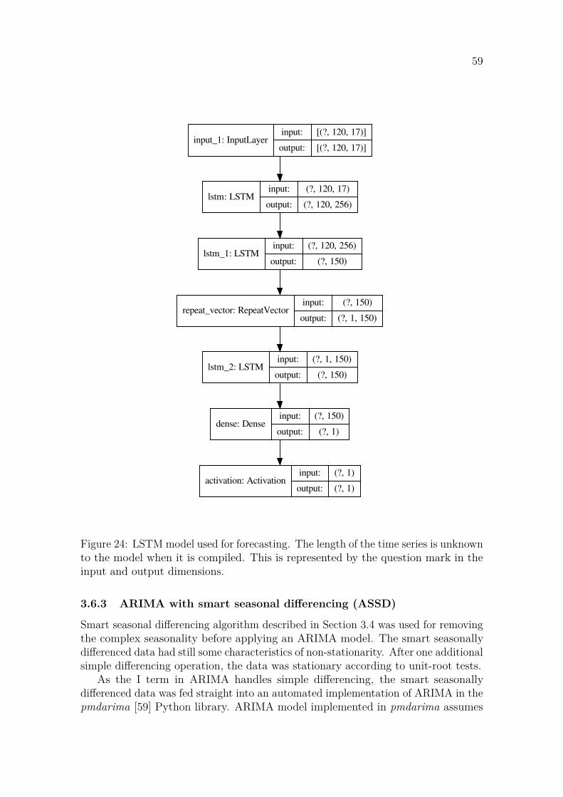
59

input_1: InputLayerinput:

output:

[(?, 120, 17)]

[(?, 120, 17)]

lstm: LSTMinput:

output:

(?, 120, 17)

(?, 120, 256)

lstm_1: LSTMinput:

output:

(?, 120, 256)

(?, 150)

repeat_vector: RepeatVectorinput:

output:

(?, 150)

(?, 1, 150)

lstm_2: LSTMinput:

output:

(?, 1, 150)

(?, 150)

dense: Denseinput:

output:

(?, 150)

(?, 1)

activation: Activationinput:

output:

(?, 1)

(?, 1)

Figure 24: LSTM model used for forecasting. The length of the time series is unknownto the model when it is compiled. This is represented by the question mark in theinput and output dimensions.

3.6.3 ARIMA with smart seasonal differencing (ASSD)

Smart seasonal differencing algorithm described in Section 3.4 was used for removingthe complex seasonality before applying an ARIMA model. The smart seasonallydifferenced data had still some characteristics of non-stationarity. After one additionalsimple differencing operation, the data was stationary according to unit-root tests.

As the I term in ARIMA handles simple differencing, the smart seasonallydifferenced data was fed straight into an automated implementation of ARIMA in thepmdarima [59] Python library. ARIMA model implemented in pmdarima assumes

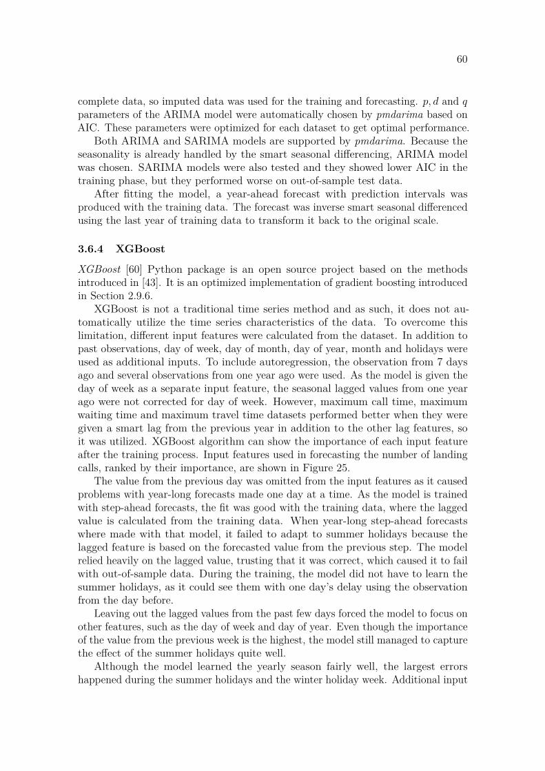
60

complete data, so imputed data was used for the training and forecasting. p, d and qparameters of the ARIMA model were automatically chosen by pmdarima based onAIC. These parameters were optimized for each dataset to get optimal performance.

Both ARIMA and SARIMA models are supported by pmdarima. Because theseasonality is already handled by the smart seasonal differencing, ARIMA modelwas chosen. SARIMA models were also tested and they showed lower AIC in thetraining phase, but they performed worse on out-of-sample test data.

After fitting the model, a year-ahead forecast with prediction intervals wasproduced with the training data. The forecast was inverse smart seasonal differencedusing the last year of training data to transform it back to the original scale.

3.6.4 XGBoost

XGBoost [60] Python package is an open source project based on the methodsintroduced in [43]. It is an optimized implementation of gradient boosting introducedin Section 2.9.6.

XGBoost is not a traditional time series method and as such, it does not au-tomatically utilize the time series characteristics of the data. To overcome thislimitation, different input features were calculated from the dataset. In addition topast observations, day of week, day of month, day of year, month and holidays wereused as additional inputs. To include autoregression, the observation from 7 daysago and several observations from one year ago were used. As the model is given theday of week as a separate input feature, the seasonal lagged values from one yearago were not corrected for day of week. However, maximum call time, maximumwaiting time and maximum travel time datasets performed better when they weregiven a smart lag from the previous year in addition to the other lag features, soit was utilized. XGBoost algorithm can show the importance of each input featureafter the training process. Input features used in forecasting the number of landingcalls, ranked by their importance, are shown in Figure 25.

The value from the previous day was omitted from the input features as it causedproblems with year-long forecasts made one day at a time. As the model is trainedwith step-ahead forecasts, the fit was good with the training data, where the laggedvalue is calculated from the training data. When year-long step-ahead forecastswhere made with that model, it failed to adapt to summer holidays because thelagged feature is based on the forecasted value from the previous step. The modelrelied heavily on the lagged value, trusting that it was correct, which caused it to failwith out-of-sample data. During the training, the model did not have to learn thesummer holidays, as it could see them with one day’s delay using the observationfrom the day before.

Leaving out the lagged values from the past few days forced the model to focus onother features, such as the day of week and day of year. Even though the importanceof the value from the previous week is the highest, the model still managed to capturethe effect of the summer holidays quite well.

Although the model learned the yearly season fairly well, the largest errorshappened during the summer holidays and the winter holiday week. Additional input

61

0 500 1000 1500 2000 2500F score

holidaytomorrow_is_holiday

yearweek_of_year

s_lag5s_lag6s_lag2s_lag3s_lag4s_lag1s_lag0

day_of_weeks_lag-7

day_of_monthday_of_year

lag7

Feat

ures

3050

233237

460462474479501514

558794

8941353

19912341

Feature importance

Figure 25: Feature importance for forecasting the number of landing calls using aXGBoost regressor. lag7 is the observation from one week ago and s_lag0 is theobservation from 52 × 7 = 364 days ago.

features were tested to see if they could improve the performance during problematicperiods of the year. Adding a summer_holiday feature which is 1 for weeks of year27-31 and 0 otherwise, showed slight improvement during the summer period. Duringweek 8 it is common to have winter holidays, as children have no school. During thewinter holiday week there is reduced traffic which is a lot higher than during officialholidays when almost no one is at work. A feature called winter_holiday was addedto improve the modeling performance during the 8th week of the year. In the end,these two additional features were removed as they could have also been added to theother models, which makes comparing the models unfair. Adding seasonal featuresis easy with domain knowledge of the building and unofficial national holidays butautomating the process in the future would be a lot more difficult.

XGBoost model is designed to handle missing data by deciding a default splittingdirection for each node if data is unavailable. This made it possible to use unimputeddatasets. When calculating the lag features, missing values were left as is. Timesteps whose data was not available, were removed altogether from the training dataas gaps in the data does not affect the model. Forecasts were made one day at a time.Date and holiday-related features were calculated for each day based on the datesof the forecast horizon. Lagged variables were calculated using the training dataand the forecasted values from previous steps of the forecasting process. The outputof the forecast was limited between zero and 1.3 × Q90%, where Q90% is the 90 %quantile of the training data. This lets the forecast to be higher than the trainingdata but prevents outliers.

62

3.7 Anomaly detectionBecause finding explanations to anomalies is easier for the past few years, 2015-2016was chosen as a training dataset and 2017 to June 2020 was used as a test dataset.Methods that do not require separate training data, were given the whole datasetfrom 2015 onwards, but only the anomalies during the test period are shown in theresults.

Anomalies existed in all the time series of the landing and DCS call datasets,but only number of calls are presented in the results. This decision was done toensure the results are as interpretable as possible. Time series that measured call,waiting and travel times are more susceptible to random events that cause anomalousobservations which are very difficult to explain afterwards. Number of calls is a fairlystable metric and also easy to understand.

Some of the anomaly detection methods required complete data, so values imputedwith the seasonal method were used with them. Anomalies detected from imputeddata were removed afterwards to ensure all anomalies were based on real observeddata.

As was expected, all the methods labeled holidays as anomalies. Days precedingholidays and Fridays following a holiday were also commonly labeled as anomalies.Anomalies were removed from the results if they happened during any of the following:

• Holiday based on a calendar

• Day before a holiday

• Friday after a holiday

• Weeks 1, 52 and 53 to filter out unofficial holidays around the New Year’s Day

• Week 8 to filter out the winter holidays

As discussed in Section 3.6.4, some of the features used for filtering are veryspecific and difficult to automate. However, they are necessary to filter out falsepositives in automatic anomaly detection.

The results were evaluated by combining the results of the different methods andcomparing the days they detected as anomalies. Explanations for the anomalies weresearched by reading old news and asking employees of the building, if they had oldcalendar events in their calendars that might explain the anomalies.

3.7.1 AnomalyDetection R package

pyculiarity [61] Python package was used instead of the AnomalyDetection [48] Rpackage. It is a ported version of the R package and the results should be the sameas with the original R package. The library advised to impute missing values soimputed datasets were used.

63

3.7.2 Rolling average and standard deviation

Rolling average and standard deviation can be used for anomaly detection. If anyobservation differs more than 1.96 × σt from the rolling average, it does not fit themodel with 95 % probability, which makes it a possible anomaly. To account forthe weekly seasonality, the rolling average and standard deviation are calculatedusing the values from the same days of week preceding and following the day tobe evaluated. While this method seems simple at first, it had some problems thatneeded to be fixed with more complicated methods.

A centered window that averages the past and following weeks, detects singleanomalous days effectively. However, it is not very effective in detecting sudden levelshifts that continue in the future. A lagging window that calculates the average ofpast weeks is more effective for such anomalies.

To find both outliers and level shifts, a centered window with 11 weeks and alagging window with 7 weeks were chosen. Both windows include the day to beevaluated, so trends caused by yearly seasonality do not cause false detection. Randomoutlier values in the data will increase the rolling standard deviation significantlywhich makes almost all observations fit inside the 95 % prediciton intervals. Tomitigate this issue, the values of the time series were limited to the 98 % quantile ofthe whole dataset, when the rolling average and standard deviation was calculated.

Many weekends were detected as anomalies if they had few more observationsthan usual. For example, 5 elevator calls on a Saturday is 67 % higher than 3 elevatorcalls on an average Saturday, but it is not likely to be an outlier as the absolutedifference is very small. These false detections were filtered out if abs(yt −yt)/y < 0.2,i.e., the absolute difference between the observed value and the rolling average wasless than 20 % of the mean of the whole time series.

Another problem with the anomalies detected with the lagging window was thatit easily picked up days during the decreasing traffic on the start of the summerholiday season. The observed values during June are a lot smaller than the 6 weeksbefore it, which is detected as an anomaly. This was fixed by filtering out anomaliesdetected with the lagging window, if the observation differed less than 10 % from thecentered rolling average. Even with this filter in place, this method detected a fewdays during the summer holidays as anomalously low, even though they seem normalwhen inspected manually. This method could probably be improved by removingthe yearly seasonality with time series decomposition.

3.7.3 ARIMA with smart seasonal differencing (ASSD)

ARIMA with smart seasonal differencing was used for forecasting in Section 3.6.3.The same model can also be used for anomaly detection by comparing the observedvalues to the prediction intervals of step-ahead predictions. Missing values wereimputed and the whole time series was smart seasonally differenced.

ARIMA model was trained with the training data using pmdarima. Anomalieswere detected by doing step-ahead predictions and updating weights of the ARIMAmodel using the observed value after each prediction. If the observed value was notinside the 95 % prediction intervals of the corresponding prediction, it was marked

64

as an anomaly. If the observed value was higher than the average of the same daysof week preceding and following it, the day was marked as higher than typical. Ifthe observed was lower than the rolling average, it was marked lower than typical.

3.7.4 tsoutliers

tsoutliers [51] R package was also tested, but its results are not shown due to poorperformance. The data used in this thesis did not suit the ARIMA model used intsoutliers, which caused problems in fitting the model. Sometimes the automatedARIMA model could not find suitable parameters to model the non-stationary data.This probably could have been corrected by using transformations like smart seasonaldifferencing. However, the anomaly detection was very slow for datasets larger thana year, which made experiments difficult. Detecting anomalies one year at a timewas not successful either, as the model detected only holidays and some extremeoutliers in the data. Longer input periods showed some improvement but with somedatasets the model did not converge after tens of minutes of calculation.

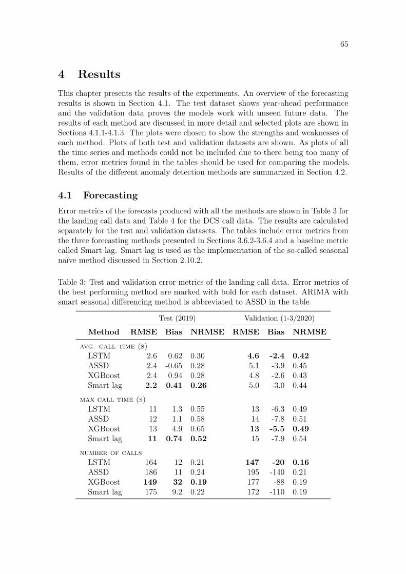
65

4 ResultsThis chapter presents the results of the experiments. An overview of the forecastingresults is shown in Section 4.1. The test dataset shows year-ahead performanceand the validation data proves the models work with unseen future data. Theresults of each method are discussed in more detail and selected plots are shown inSections 4.1.1-4.1.3. The plots were chosen to show the strengths and weaknesses ofeach method. Plots of both test and validation datasets are shown. As plots of allthe time series and methods could not be included due to there being too many ofthem, error metrics found in the tables should be used for comparing the models.Results of the different anomaly detection methods are summarized in Section 4.2.

4.1 ForecastingError metrics of the forecasts produced with all the methods are shown in Table 3 forthe landing call data and Table 4 for the DCS call data. The results are calculatedseparately for the test and validation datasets. The tables include error metrics fromthe three forecasting methods presented in Sections 3.6.2-3.6.4 and a baseline metriccalled Smart lag. Smart lag is used as the implementation of the so-called seasonalnaïve method discussed in Section 2.10.2.

Table 3: Test and validation error metrics of the landing call data. Error metrics ofthe best performing method are marked with bold for each dataset. ARIMA withsmart seasonal differencing method is abbreviated to ASSD in the table.

Test (2019) Validation (1-3/2020)

Method RMSE Bias NRMSE RMSE Bias NRMSEavg. call time (s)

LSTM 2.6 0.62 0.30 4.6 -2.4 0.42ASSD 2.4 -0.65 0.28 5.1 -3.9 0.45XGBoost 2.4 0.94 0.28 4.8 -2.6 0.43Smart lag 2.2 0.41 0.26 5.0 -3.0 0.44

max call time (s)LSTM 11 1.3 0.55 13 -6.3 0.49ASSD 12 1.1 0.58 14 -7.8 0.51XGBoost 13 4.9 0.65 13 -5.5 0.49Smart lag 11 0.74 0.52 15 -7.9 0.54

number of callsLSTM 164 12 0.21 147 -20 0.16ASSD 186 11 0.24 195 -140 0.21XGBoost 149 32 0.19 177 -88 0.19Smart lag 175 9.2 0.22 172 -110 0.19

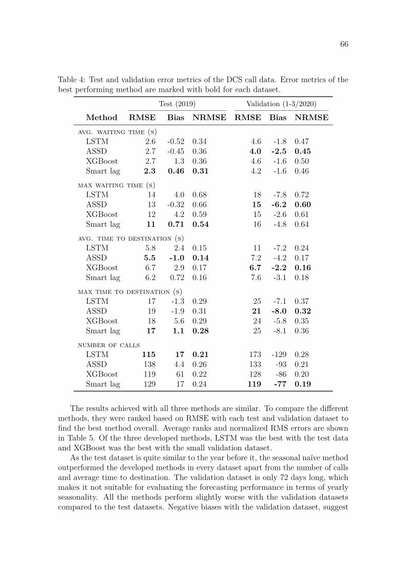
66

Table 4: Test and validation error metrics of the DCS call data. Error metrics of thebest performing method are marked with bold for each dataset.

Test (2019) Validation (1-3/2020)

Method RMSE Bias NRMSE RMSE Bias NRMSEavg. waiting time (s)

LSTM 2.6 -0.52 0.34 4.6 -1.8 0.47ASSD 2.7 -0.45 0.36 4.0 -2.5 0.45XGBoost 2.7 1.3 0.36 4.6 -1.6 0.50Smart lag 2.3 0.46 0.31 4.2 -1.6 0.46

max waiting time (s)LSTM 14 4.0 0.68 18 -7.8 0.72ASSD 13 -0.32 0.66 15 -6.2 0.60XGBoost 12 4.2 0.59 15 -2.6 0.61Smart lag 11 0.71 0.54 16 -4.8 0.64

avg. time to destination (s)LSTM 5.8 2.4 0.15 11 -7.2 0.24ASSD 5.5 -1.0 0.14 7.2 -4.2 0.17XGBoost 6.7 2.9 0.17 6.7 -2.2 0.16Smart lag 6.2 0.72 0.16 7.6 -3.1 0.18

max time to destination (s)LSTM 17 -1.3 0.29 25 -7.1 0.37ASSD 19 -1.9 0.31 21 -8.0 0.32XGBoost 18 5.6 0.29 24 -5.8 0.35Smart lag 17 1.1 0.28 25 -8.1 0.36

number of callsLSTM 115 17 0.21 173 -129 0.28ASSD 138 4.4 0.26 133 -93 0.21XGBoost 119 61 0.22 128 -86 0.20Smart lag 129 17 0.24 119 -77 0.19

The results achieved with all three methods are similar. To compare the differentmethods, they were ranked based on RMSE with each test and validation dataset tofind the best method overall. Average ranks and normalized RMS errors are shownin Table 5. Of the three developed methods, LSTM was the best with the test dataand XGBoost was the best with the small validation dataset.

As the test dataset is quite similar to the year before it, the seasonal naïve methodoutperformed the developed methods in every dataset apart from the number of callsand average time to destination. The validation dataset is only 72 days long, whichmakes it not suitable for evaluating the forecasting performance in terms of yearlyseasonality. All the methods perform slightly worse with the validation datasetscompared to the test datasets. Negative biases with the validation dataset, suggest

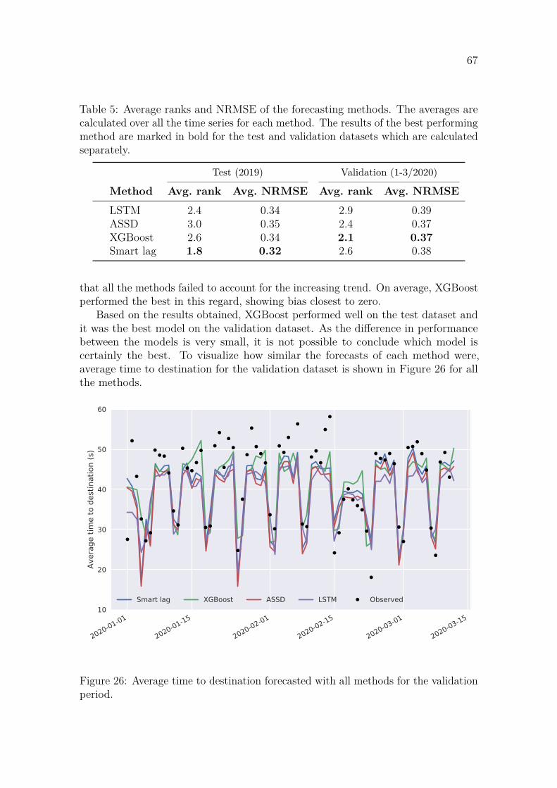
67

Table 5: Average ranks and NRMSE of the forecasting methods. The averages arecalculated over all the time series for each method. The results of the best performingmethod are marked in bold for the test and validation datasets which are calculatedseparately.

Test (2019) Validation (1-3/2020)

Method Avg. rank Avg. NRMSE Avg. rank Avg. NRMSELSTM 2.4 0.34 2.9 0.39ASSD 3.0 0.35 2.4 0.37XGBoost 2.6 0.34 2.1 0.37Smart lag 1.8 0.32 2.6 0.38

that all the methods failed to account for the increasing trend. On average, XGBoostperformed the best in this regard, showing bias closest to zero.

Based on the results obtained, XGBoost performed well on the test dataset andit was the best model on the validation dataset. As the difference in performancebetween the models is very small, it is not possible to conclude which model iscertainly the best. To visualize how similar the forecasts of each method were,average time to destination for the validation dataset is shown in Figure 26 for allthe methods.

2020-01-01

2020-01-15

2020-02-01

2020-02-15

2020-03-01

2020-03-1510

20

30

40

50

60

Aver

age

time

to d

estin

atio

n (s

)

Smart lag XGBoost ASSD LSTM Observed

Figure 26: Average time to destination forecasted with all methods for the validationperiod.

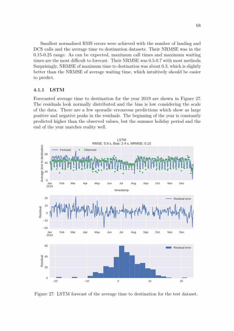
68

Smallest normalized RMS errors were achieved with the number of landing andDCS calls and the average time to destination datasets. Their NRMSE was in the0.15-0.25 range. As can be expected, maximum call times and maximum waitingtimes are the most difficult to forecast. Their NRMSE was 0.5-0.7 with most methods.Surprisingly, NRMSE of maximum time to destination was about 0.3, which is slightlybetter than the NRMSE of average waiting time, which intuitively should be easierto predict.

4.1.1 LSTM

Forecasted average time to destination for the year 2019 are shown in Figure 27.The residuals look normally distributed and the bias is low considering the scaleof the data. There are a few sporadic erroneous predictions which show as largepositive and negative peaks in the residuals. The beginning of the year is constantlypredicted higher than the observed values, but the summer holiday period and theend of the year matches reality well.

Jan2019

Feb Mar Apr May Jun Jul Aug Sep Oct Nov Dec

timestamp

0

20

40

60

Ave

rage

tim

e to

des

tinat

ion

LSTMRMSE: 5.8 s, Bias: 2.4 s, NRMSE: 0.15

Forecast Observed

Jan2019

Feb Mar Apr May Jun Jul Aug Sep Oct Nov Dec20

10

0

10

20

Res

idua

l

Residual error

20 10 0 10 200

20

40

60

Res

idua

l

Residual error

Figure 27: LSTM forecast of the average time to destination for the test dataset.

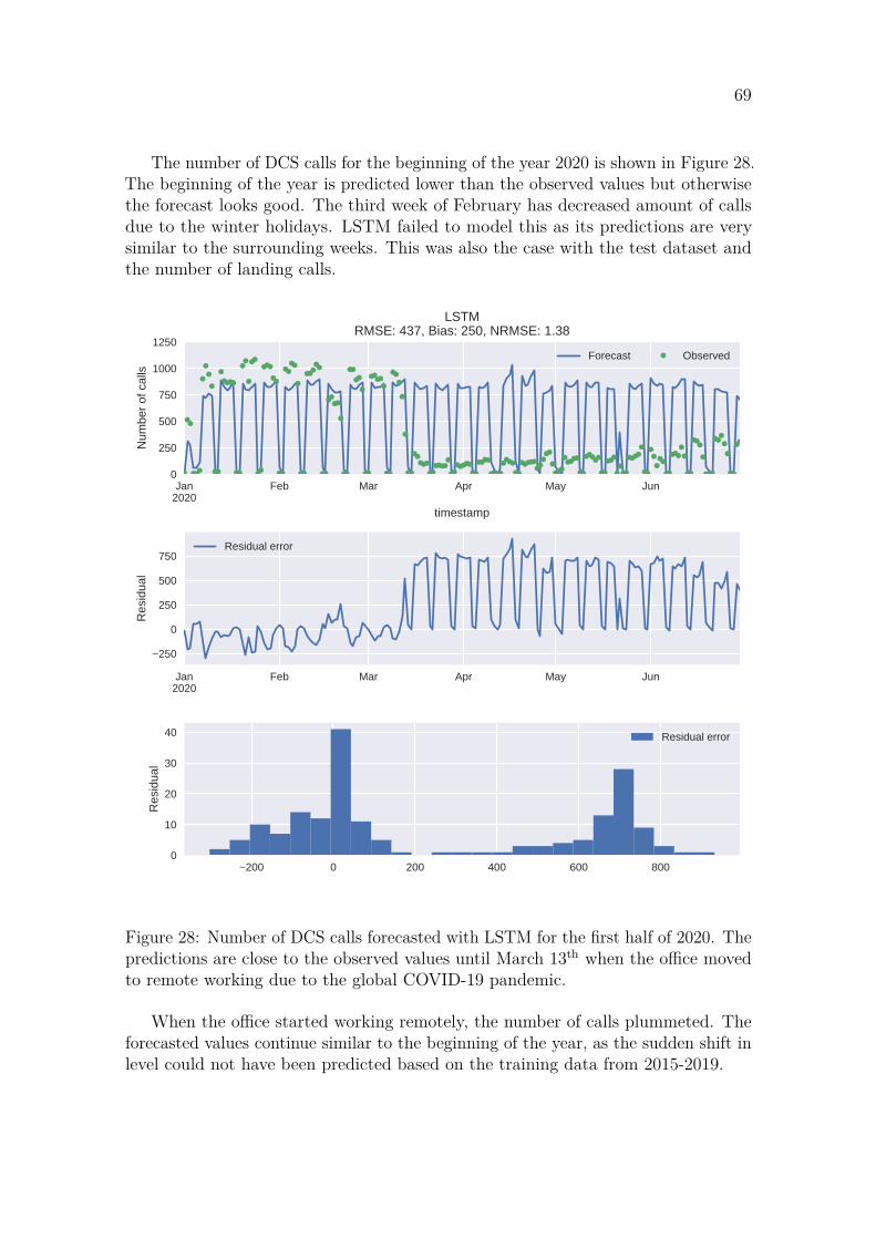
69

The number of DCS calls for the beginning of the year 2020 is shown in Figure 28.The beginning of the year is predicted lower than the observed values but otherwisethe forecast looks good. The third week of February has decreased amount of callsdue to the winter holidays. LSTM failed to model this as its predictions are verysimilar to the surrounding weeks. This was also the case with the test dataset andthe number of landing calls.

Jan2020

Feb Mar Apr May Jun

timestamp

0

250

500

750

1000

1250

Num

ber o

f cal

ls

LSTMRMSE: 437, Bias: 250, NRMSE: 1.38

Forecast Observed

Jan2020

Feb Mar Apr May Jun

250

0

250

500

750

Res

idua

l

Residual error

200 0 200 400 600 8000

10

20

30

40

Res

idua

l

Residual error

Figure 28: Number of DCS calls forecasted with LSTM for the first half of 2020. Thepredictions are close to the observed values until March 13th when the office movedto remote working due to the global COVID-19 pandemic.

When the office started working remotely, the number of calls plummeted. Theforecasted values continue similar to the beginning of the year, as the sudden shift inlevel could not have been predicted based on the training data from 2015-2019.

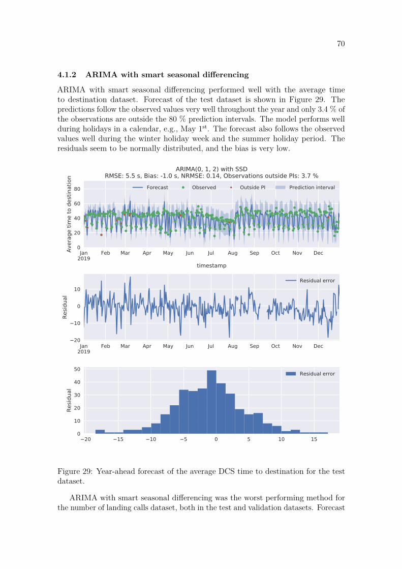
70

4.1.2 ARIMA with smart seasonal differencing

ARIMA with smart seasonal differencing performed well with the average timeto destination dataset. Forecast of the test dataset is shown in Figure 29. Thepredictions follow the observed values very well throughout the year and only 3.4 % ofthe observations are outside the 80 % prediction intervals. The model performs wellduring holidays in a calendar, e.g., May 1st. The forecast also follows the observedvalues well during the winter holiday week and the summer holiday period. Theresiduals seem to be normally distributed, and the bias is very low.

Jan2019

Feb Mar Apr May Jun Jul Aug Sep Oct Nov Dec

timestamp

0

20

40

60

80

Aver

age

time

to d

estin

atio

n

ARIMA(0, 1, 2) with SSDRMSE: 5.5 s, Bias: -1.0 s, NRMSE: 0.14, Observations outside PIs: 3.7 %

Forecast Observed Outside PI Prediction interval

Jan2019

Feb Mar Apr May Jun Jul Aug Sep Oct Nov Dec20

10

0

10

Resid

ual

Residual error

20 15 10 5 0 5 10 150

10

20

30

40

50

Resid

ual

Residual error

Figure 29: Year-ahead forecast of the average DCS time to destination for the testdataset.

ARIMA with smart seasonal differencing was the worst performing method forthe number of landing calls dataset, both in the test and validation datasets. Forecast

71

for the test dataset is shown in Figure 30. Even though this was the worst method,the forecast looks good. It managed to account for the winter and summer holidayswell and the level of the forecast is close to the observations during the whole year.

Even though the forecast looks good overall, there are some extremely highoutliers on December 5th, 23rd, 30th and 31st. They are days preceding a holidaywhich has caused people to work from home. As the days are not in the holidaycalendar, they were modeled as regular days, which caused the forecast to be a lothigher than the observed value. Interestingly, December 5th is an exception as it wasforecasted to be quiet, but in reality it had quite normal traffic.

Number of calls for Friday February 1st was forecasted quite low even thoughthere were no holidays in February or late January. After investigating the issue,a reasonable explanation was found. Due to the smart seasonal differencing, theprediction is largely based on Friday February 2nd 2018, which had unusually lowamount of landing calls. That day, there were multiple strikes including bus drivers.It is likely that some employees had to work from home because public transportationwas not available. Such issues could be solved by not using abnormal days as smartlag values. Detecting abnormal days could be achieved by utilizing the anomalydetection methods described in Section 2.11.

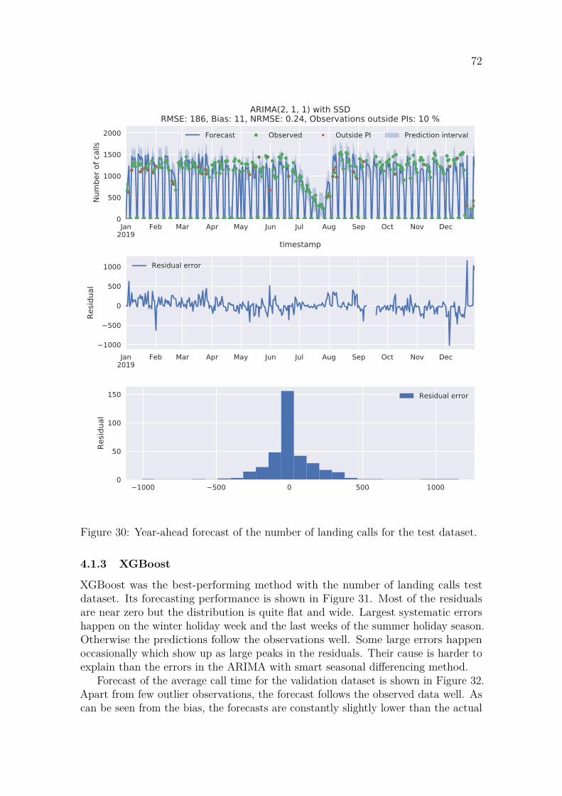
72

Jan2019

Feb Mar Apr May Jun Jul Aug Sep Oct Nov Dec

timestamp

0

500

1000

1500

2000

Num

ber o

f cal

lsARIMA(2, 1, 1) with SSD

RMSE: 186, Bias: 11, NRMSE: 0.24, Observations outside PIs: 10 %Forecast Observed Outside PI Prediction interval

Jan2019

Feb Mar Apr May Jun Jul Aug Sep Oct Nov Dec1000

500

0

500

1000

Resid

ual

Residual error

1000 500 0 500 10000

50

100

150

Resid

ual

Residual error

Figure 30: Year-ahead forecast of the number of landing calls for the test dataset.

4.1.3 XGBoost

XGBoost was the best-performing method with the number of landing calls testdataset. Its forecasting performance is shown in Figure 31. Most of the residualsare near zero but the distribution is quite flat and wide. Largest systematic errorshappen on the winter holiday week and the last weeks of the summer holiday season.Otherwise the predictions follow the observations well. Some large errors happenoccasionally which show up as large peaks in the residuals. Their cause is harder toexplain than the errors in the ARIMA with smart seasonal differencing method.

Forecast of the average call time for the validation dataset is shown in Figure 32.Apart from few outlier observations, the forecast follows the observed data well. Ascan be seen from the bias, the forecasts are constantly slightly lower than the actual

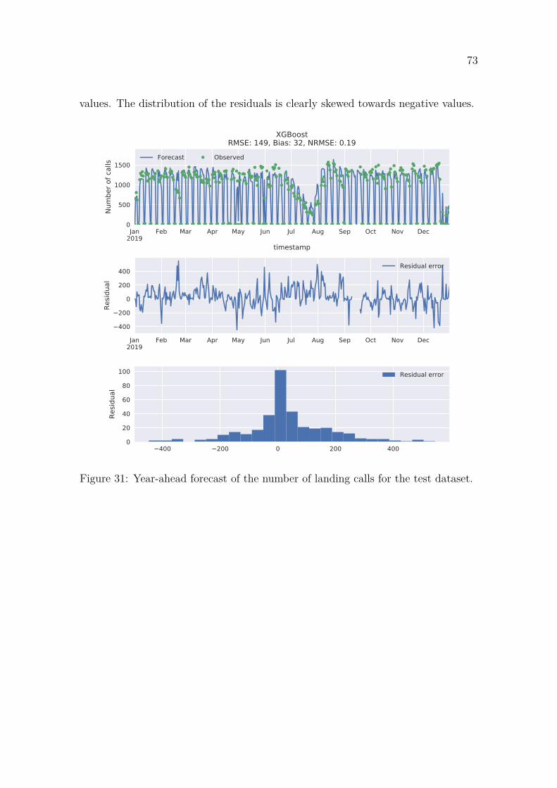
73

values. The distribution of the residuals is clearly skewed towards negative values.

Jan2019

Feb Mar Apr May Jun Jul Aug Sep Oct Nov Dec

timestamp

0

500

1000

1500

Num

ber o

f cal

ls

XGBoostRMSE: 149, Bias: 32, NRMSE: 0.19

Forecast Observed

Jan2019

Feb Mar Apr May Jun Jul Aug Sep Oct Nov Dec

400

200

0

200

400

Resid

ual

Residual error

400 200 0 200 4000

20

40

60

80

100

Resid

ual

Residual error

Figure 31: Year-ahead forecast of the number of landing calls for the test dataset.

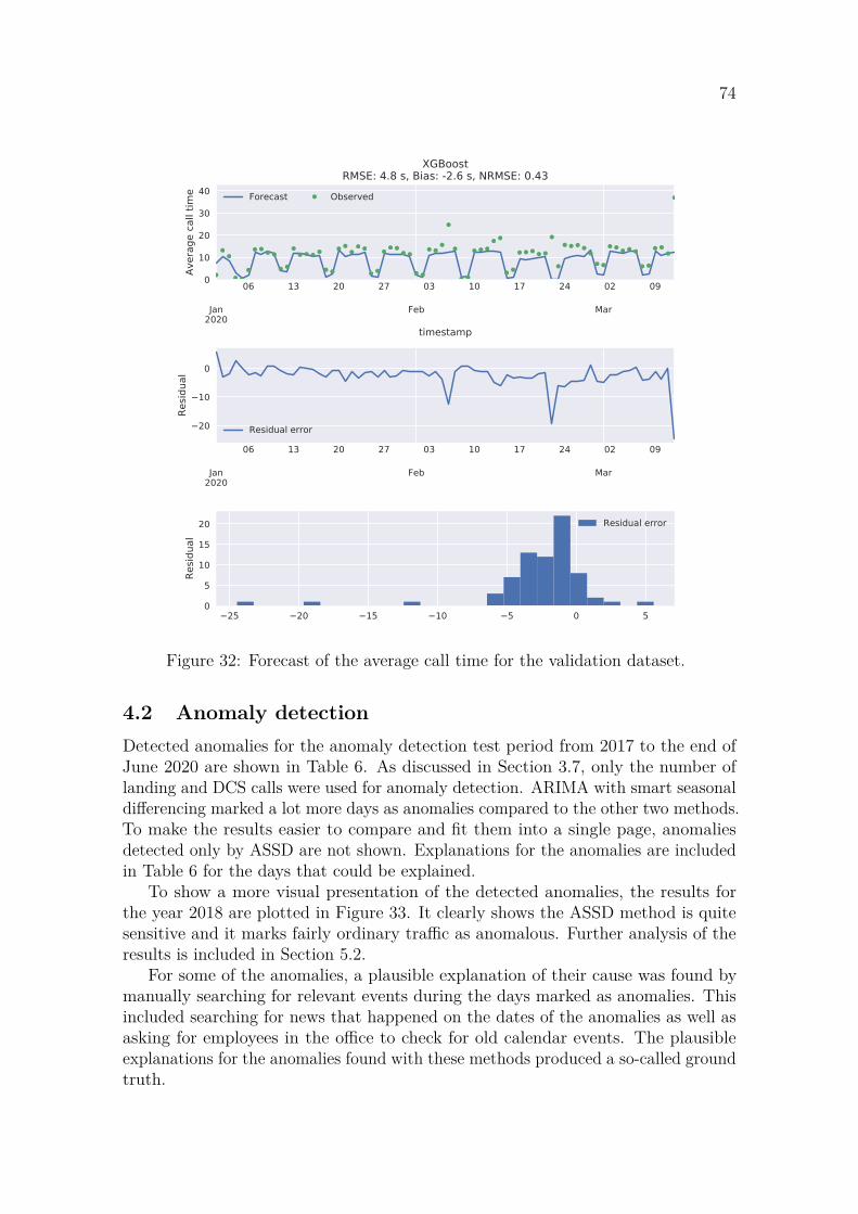
74

Jan2020

Feb Mar

06 13 20 27 03 10 17 24 02 09

timestamp

0

10

20

30

40Av

erag

e ca

ll tim

e

XGBoostRMSE: 4.8 s, Bias: -2.6 s, NRMSE: 0.43

Forecast Observed

Jan2020

Feb Mar

06 13 20 27 03 10 17 24 02 09

20

10

0

Resid

ual

Residual error

25 20 15 10 5 0 50

5

10

15

20

Resid

ual

Residual error

Figure 32: Forecast of the average call time for the validation dataset.

4.2 Anomaly detectionDetected anomalies for the anomaly detection test period from 2017 to the end ofJune 2020 are shown in Table 6. As discussed in Section 3.7, only the number oflanding and DCS calls were used for anomaly detection. ARIMA with smart seasonaldifferencing marked a lot more days as anomalies compared to the other two methods.To make the results easier to compare and fit them into a single page, anomaliesdetected only by ASSD are not shown. Explanations for the anomalies are includedin Table 6 for the days that could be explained.

To show a more visual presentation of the detected anomalies, the results forthe year 2018 are plotted in Figure 33. It clearly shows the ASSD method is quitesensitive and it marks fairly ordinary traffic as anomalous. Further analysis of theresults is included in Section 5.2.

For some of the anomalies, a plausible explanation of their cause was found bymanually searching for relevant events during the days marked as anomalies. Thisincluded searching for news that happened on the dates of the anomalies as well asasking for employees in the office to check for old calendar events. The plausibleexplanations for the anomalies found with these methods produced a so-called groundtruth.

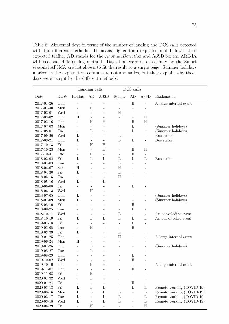
75

Table 6: Abnormal days in terms of the number of landing and DCS calls detectedwith the different methods. H means higher than expected and L lower thanexpected traffic. AD stands for the AnomalyDetection and ASSD for the ARIMAwith seasonal differencing method. Days that were detected only by the Smartseasonal ARIMA are not shown to fit the result to a single page. Summer holidaysmarked in the explanation column are not anomalies, but they explain why thosedays were caught by the different methods.

Landing calls DCS callsDate DOW Rolling AD ASSD Rolling AD ASSD Explanation

2017-01-26 Thu - - - - H - A large internal event2017-01-30 Mon - H - - - -2017-03-01 Wed - - - H - -2017-03-02 Thu H - - - - H2017-03-16 Thu - H H - H H2017-07-03 Mon - - - - L - (Summer holidays)2017-08-01 Tue - L - - L - (Summer holidays)2017-09-20 Wed L L - L - - Bus strike2017-09-21 Thu L - - L L - Bus strike2017-10-13 Fri - H H - - -2017-10-23 Mon - - H - H H2017-10-31 Tue - H - - H -2018-02-02 Fri L L L L L L Bus strike2018-04-03 Tue - - - L - -2018-04-07 Sat H - - H - -2018-04-20 Fri L - - L - -2018-05-15 Tue - - - H - -2018-05-16 Wed L - L - - -2018-06-08 Fri - - - - L -2018-06-13 Wed - H - - - -2018-07-05 Thu L - - - - - (Summer holidays)2018-07-09 Mon L - - - - - (Summer holidays)2018-08-10 Fri - - - - H -2018-09-25 Tue - L - - L -2018-10-17 Wed - - - L - - An out-of-office event2018-10-19 Fri L L L L L L An out-of-office event2019-01-18 Fri - - - - L -2019-03-05 Tue - H - - H -2019-03-29 Fri L - - L - -2019-04-25 Thu - - - H - - A large internal event2019-06-24 Mon H - - - - -2019-07-25 Thu - L - - - - (Summer holidays)2019-08-27 Tue - L - - - -2019-08-29 Thu - - - - L -2019-10-02 Wed - - - - H -2019-10-10 Thu - H H - - - A large internal event2019-11-07 Thu - - - - H -2019-11-08 Fri - H - - - -2020-01-22 Wed - L - - - -2020-01-24 Fri - - - - H -2020-03-13 Fri L L L - L L Remote working (COVID-19)2020-03-16 Mon L L L L - L Remote working (COVID-19)2020-03-17 Tue L - L L - L Remote working (COVID-19)2020-03-18 Wed L - L L - L Remote working (COVID-19)2020-05-29 Fri - H - - - H

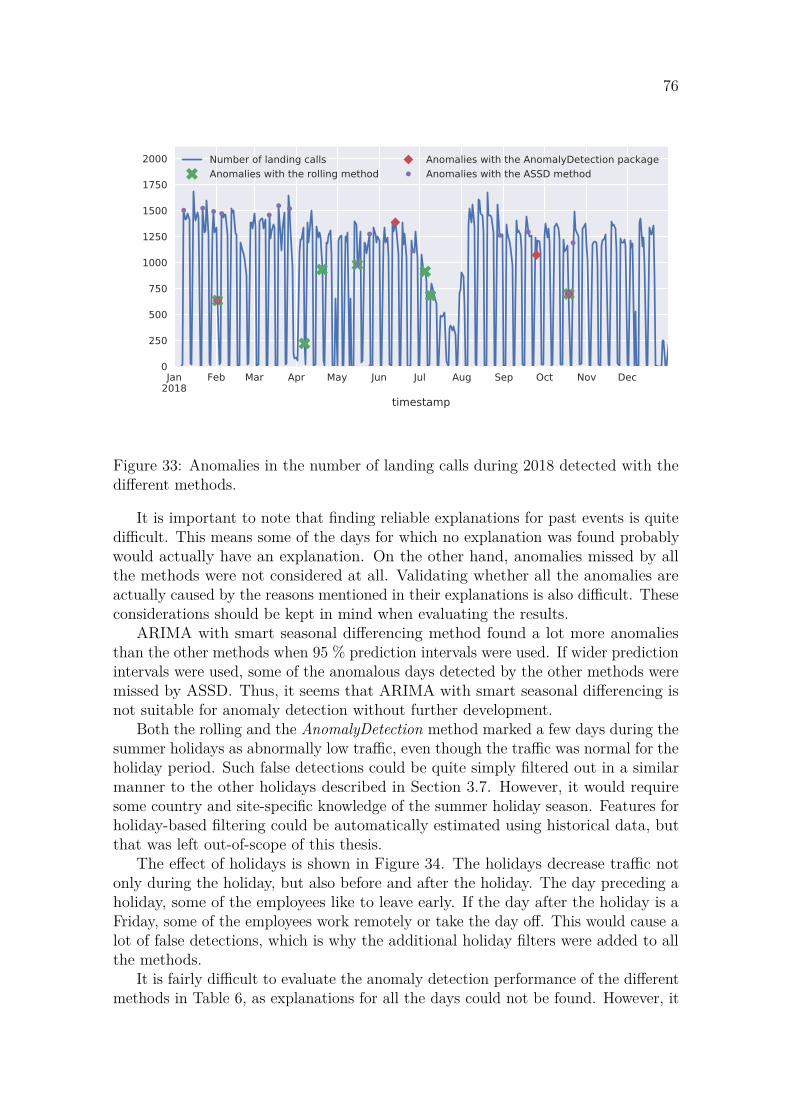
76

Jan2018

Feb Mar Apr May Jun Jul Aug Sep Oct Nov Dec

timestamp

0

250

500

750

1000

1250

1500

1750

2000 Number of landing callsAnomalies with the rolling method

Anomalies with the AnomalyDetection packageAnomalies with the ASSD method

Figure 33: Anomalies in the number of landing calls during 2018 detected with thedifferent methods.

It is important to note that finding reliable explanations for past events is quitedifficult. This means some of the days for which no explanation was found probablywould actually have an explanation. On the other hand, anomalies missed by allthe methods were not considered at all. Validating whether all the anomalies areactually caused by the reasons mentioned in their explanations is also difficult. Theseconsiderations should be kept in mind when evaluating the results.

ARIMA with smart seasonal differencing method found a lot more anomaliesthan the other methods when 95 % prediction intervals were used. If wider predictionintervals were used, some of the anomalous days detected by the other methods weremissed by ASSD. Thus, it seems that ARIMA with smart seasonal differencing isnot suitable for anomaly detection without further development.

Both the rolling and the AnomalyDetection method marked a few days during thesummer holidays as abnormally low traffic, even though the traffic was normal for theholiday period. Such false detections could be quite simply filtered out in a similarmanner to the other holidays described in Section 3.7. However, it would requiresome country and site-specific knowledge of the summer holiday season. Features forholiday-based filtering could be automatically estimated using historical data, butthat was left out-of-scope of this thesis.

The effect of holidays is shown in Figure 34. The holidays decrease traffic notonly during the holiday, but also before and after the holiday. The day preceding aholiday, some of the employees like to leave early. If the day after the holiday is aFriday, some of the employees work remotely or take the day off. This would cause alot of false detections, which is why the additional holiday filters were added to allthe methods.

It is fairly difficult to evaluate the anomaly detection performance of the differentmethods in Table 6, as explanations for all the days could not be found. However, it

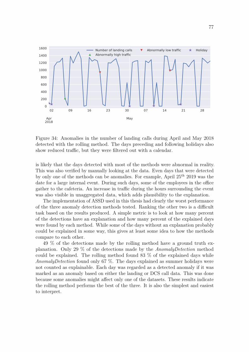
77

Apr2018

May

02 09 16 23 30 07 14 21 28

ds

0

200

400

600

800

1000

1200

1400

1600 Number of landing callsAbnormally high traffic

Abnormally low traffic Holiday

Figure 34: Anomalies in the number of landing calls during April and May 2018detected with the rolling method. The days preceding and following holidays alsoshow reduced traffic, but they were filtered out with a calendar.

is likely that the days detected with most of the methods were abnormal in reality.This was also verified by manually looking at the data. Even days that were detectedby only one of the methods can be anomalies. For example, April 25th 2019 was thedate for a large internal event. During such days, some of the employees in the officegather to the cafeteria. An increase in traffic during the hours surrounding the eventwas also visible in unaggregated data, which adds plausibility to the explanation.

The implementation of ASSD used in this thesis had clearly the worst performanceof the three anomaly detection methods tested. Ranking the other two is a difficulttask based on the results produced. A simple metric is to look at how many percentof the detections have an explanation and how many percent of the explained dayswere found by each method. While some of the days without an explanation probablycould be explained in some way, this gives at least some idea to how the methodscompare to each other.

49 % of the detections made by the rolling method have a ground truth ex-planation. Only 29 % of the detections made by the AnomalyDetection methodcould be explained. The rolling method found 83 % of the explained days whileAnomalyDetection found only 67 %. The days explained as summer holidays werenot counted as explainable. Each day was regarded as a detected anomaly if it wasmarked as an anomaly based on either the landing or DCS call data. This was donebecause some anomalies might affect only one of the datasets. These results indicatethe rolling method performs the best of the three. It is also the simplest and easiestto interpret.

78

5 DiscussionThis chapter includes a discussion of the results. Section 5.1 reviews which of the goalsset for forecasting were met and which require more work in the future. Section 5.2examines the validity of the anomaly detection results and outlines a few ideas forfuture development.

5.1 ForecastingOne of the goals for the models developed in this thesis was to model the complexseasonality present in the data. Based on the forecasts produced by all the models,this goal was met. The year-ahead predictions followed the weekly and yearlyseasonalities well, and even holidays were modeled correctly in most cases.

Another goal was to produce long-term forecasts of elevator usage and peopleflow performance. Such forecasts would be useful in ensuring optimal people flow inbuildings throughout their life cycles. Large negative biases in the forecasts of thevalidation set indicate none of the methods managed to predict the increasing trend.Modeling the relatively small trend component in the datasets was shadowed by thecomplex seasonality, which took a lot of time and effort to model successfully.

The failure to predict the trend in the chosen models was caused by multiplereasons. The trend in elevator traffic data is non-deterministic and modeling it isdifficult, especially with a very limited amount of data. The ARIMA model usedin the ASSD method was given smart seasonally differenced data as its input. TheARIMA model assumed its input data to be stationary or stationary after differencing,i.e., it has no trend, or the trend is constant. As the forecasts produced for the testdataset did not seem to clearly suffer from the lack of a trend component, it was notadded during the development. XGBoost and LSTM models were given the year andmonth of the observations as input features. They could have learned the trend, butboth underperformed with the validation dataset.

Based on the validation results, the trend component should have been researchedmore and possibly modeled separately. However, due to lack of time and data itwas not done in this thesis. If the models would have been tuned to forecast thevalidation datasets, it would be uncertain if they would work any better with unseenfuture data.

Working with daily data added complexity to the models as they had to copewith multiple seasonality. Using weekly or monthly aggregated data could havesimplified the modeling task and possibly enabled the models to learn the trendcomponent better. Another option would have been to extract the trend using timeseries decomposition and forecast it separately. This would possibly be a quick andstraight-forward way to improve the developed models and make them more usablefor predicting future traffic demand. Due to time constraints, such experiments wereleft out of this thesis, but it would be a good starting point for future research.

While based on the results of the experiment, XGBoost was concluded as thebest-performing method, the results cannot be generalized. The test and validationdatasets were quite short and only from a single office building. In addition, random

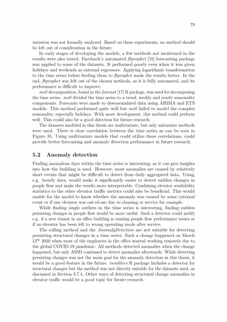
79

variation was not formally analyzed. Based on these experiments, no method shouldbe left out of consideration in the future.

In early stages of developing the models, a few methods not mentioned in theresults were also tested. Facebook’s automated fbprophet [55] forecasting packagewas applied to some of the datasets. It performed poorly even when it was givenholidays and weekends as external regressors. Applying logarithmic transformationto the time series before feeding them to fbprophet made the results better. In theend, fbprophet was left out of the chosen methods, as it is fully automated, and itsperformance is difficult to improve.

mstl decomposition, found in the forecast [17] R package, was used for decomposingthe time series. mstl divided the time series to a trend, weekly and yearly seasonalitycomponents. Forecasts were made to deseasonalized data using ARIMA and ETSmodels. This method performed quite well but mstl failed to model the complexseasonality, especially holidays. With more development, this method could performwell. This could also be a good direction for future research.

The datasets modeled in this thesis are multivariate, but only univariate methodswere used. There is clear correlation between the time series as can be seen inFigure 35. Using multivariate models that could utilize these correlations, couldprovide better forecasting and anomaly detection performance in future research.

5.2 Anomaly detectionFinding anomalous days within the time series is interesting, as it can give insightsinto how the building is used. However, most anomalies are caused by relativelyshort events that might be difficult to detect from daily aggregated data. Using,e.g. hourly data, would make it significantly easier to detect sudden changes inpeople flow and make the results more interpretable. Combining elevator availabilitystatistics to the other elevator traffic metrics could also be beneficial. This wouldenable for the model to know whether the anomaly was caused by some externalevent or if one elevator was out-of-use due to cleaning or service for example.

While finding single outliers in the time series is interesting, finding suddenpersisting changes in people flow would be more useful. Such a detector could notifye.g. if a new tenant in an office building is causing people flow performance issues orif an elevator has been left to wrong operating mode after service.

The rolling method and the AnomalyDetection are not suitable for detectingpersisting structural changes in a time series. Such a change happened on March13th 2020 when most of the employees in the office started working remotely due tothe global COVID-19 pandemic. All methods detected anomalies when the changehappened, but only ASSD continued to detect anomalies afterwards. While detectingpersisting changes was not the main goal for the anomaly detection in this thesis, itwould be a good feature in the future. tsoutliers R package includes a detector forstructural changes but the method was not directly suitable for the datasets used, asdiscussed in Section 3.7.4. Other ways of detecting structural change anomalies inelevator traffic would be a good topic for future research.

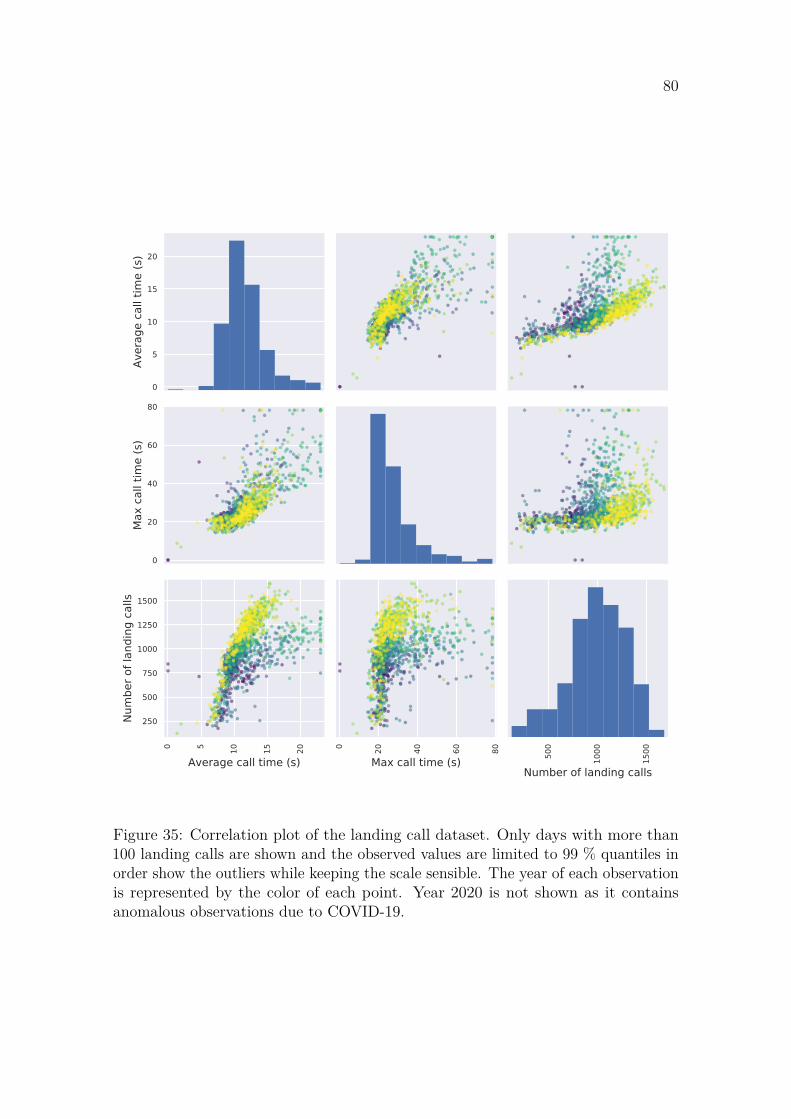
80

0

5

10

15

20

Aver

age

call

time

(s)

0

20

40

60

80

Max

cal

l tim

e (s

)

0 5 10 15 20

Average call time (s)

250

500

750

1000

1250

1500

Num

ber o

f lan

ding

cal

ls

0 20 40 60 80

Max call time (s) 500

1000

1500

Number of landing calls

Figure 35: Correlation plot of the landing call dataset. Only days with more than100 landing calls are shown and the observed values are limited to 99 % quantiles inorder show the outliers while keeping the scale sensible. The year of each observationis represented by the color of each point. Year 2020 is not shown as it containsanomalous observations due to COVID-19.

81

6 ConclusionsThe elevator traffic datasets used in this thesis were thoroughly explored to findout their characteristic features. They show strong weekly and yearly seasonalities,which complicate the modeling process. Due to technical and human errors, some ofthe data is missing. External factors affect the behavior of office employees, whichshow up as anomalies in people flow data. All these factors were considered whenthe modeling methods used were developed.

The time series models developed in this thesis were successful in capturingthe complex multiple seasonality present in elevator traffic datasets. In addition, anew imputation method was developed based on the strengths and weaknesses ofexisting implementations. It imputes missing data considering the seasonality andeffects caused by holidays. The imputed data was used for forecasting and anomalydetection models that require complete data.

The modeling methods applied to the datasets were developed based on theinformation gathered with a literature review on time series data and modeling.While the methods applied were mostly existing implementations found in varioussoftware packages, the input data required transformations and processing to makeit work with the models. Smart lag operator and smart seasonal differencing weredeveloped in this thesis to help the models cope with the complex seasonality.

Year-ahead forecasts produced with all the developed models follow out-of-sampleobservations well, proving that long-term predictions are possible. Two of the models,i.e. ASSD and XGBoost, outperformed the baseline model with validation data. Themodels did not completely capture trends present in the datasets. Modeling thetrends separately from the seasonality would be a good direction for future research.Although the models had some weaknesses, the results show that it is possible towork with elevator traffic time series aggregated to daily level, even with long forecasthorizons.

Four different anomaly detection algorithms were applied to some of the timeseries datasets. Two of them were successful in detecting clear anomalies in elevatortraffic. For some of these anomalies, an explanation was found to help validatethe results obtained. Finding short-term anomalies could possibly benefit fromusing hourly datasets and adding elevator availability statistics as external variables.Future research could focus on detecting persisting long-term changes in people flowdata which would be helpful in detecting problems automatically.

The findings and results of this thesis are a good foundation for future develop-ments in time series modeling of elevator traffic data. It is clear that people flow datashould be recorded and archived for future use. With some more work in the future,time series analysis could be automated fleet-wide, which would yield invaluableinsights into the usage of the buildings throughout their life cycles. People flow datais something few organizations can acquire, which makes it very valuable. Datagathered today will give a competitive advantage in the future, when it can be fullyutilized.

82

References[1] Marja-Liisa Siikonen and Janne Sorsa. People Flow Analysis in Lift

Modernization. In 8th Symposium on Lift & Escalator Technologies/CIBSE,pages 89–98, May 2018.

[2] Marja-Liisa Siikonen and J. Leppälä. Elevator traffic pattern recognition. InProceedings of IFSA ’91 Brussels, pages 195–198. The Internationasl FuzzySystems Association, July 1991.

[3] Xiaoke Yan, Yu Liu, Zongyuan Mao, Zhong-Hua Li, and Hong-Zhou Tan.SVM-based Elevator Traffic Flow Prediction. In 2006 6th World Congress onIntelligent Control and Automation, volume 2, pages 8814–8818, June 2006.doi: 10.1109/WCICA.2006.1713703.

[4] Erkan Erdogdu. Electricity demand analysis using cointegration and ARIMAmodelling: A case study of Turkey. Energy Policy, 35(2):1129–1146, February2007. ISSN 0301-4215. doi: 10.1016/j.enpol.2006.02.013.

[5] Ergun Yukseltan, Ahmet Yucekaya, and Ayse Humeyra Bilge. Forecastingelectricity demand for Turkey: Modeling periodic variations and demandsegregation. Applied Energy, 193:287–296, May 2017. ISSN 0306-2619. doi:10.1016/j.apenergy.2017.02.054.

[6] Raquel Prado and Mike West. Time Series: Modeling, Computation, andInference. CRC Press LLC, Philadelphia, PA, United States, 2010. ISBN978-1-4398-8275-7.

[7] Peter J. Brockwell and Richard A. Davis. Introduction to Time Series andForecasting. Springer Texts in Statistics. Springer, New York, second edition,2002. ISBN 978-0-387-95351-9.

[8] Peter J. Brockwell. Time Series: Theory and Methods. Springer Series inStatistics. Springer, second edition, 1991.

[9] R.J. Hyndman and G. Athanasopoulos. Forecasting: Principles and practice,2nd edition, OTexts: Melbourne, Australia. https://otexts.com/fpp2/, 2018.

[10] George E. P. Box, Gwilym M. Jenkins, and Gregory C. Reinsel. Time SeriesAnalysis. John Wiley & Sons, Ltd, fourth edition, 2008. ISBN978-1-118-61919-3. doi: 10.1002/9781118619193.

[11] Robert H. Shumway and David S. Stoffer. Time Series Analysis and ItsApplications: With R Examples. Springer, April 2017. ISBN 978-3-319-52452-8.

[12] Evžen Kočenda and Alexandr Černý. Elements of Time Series Econometrics:An Applied Approach. Karolinum Press, Prague, Czech Republic, secondedition, 2015. ISBN 978-80-246-3198-1.

83

[13] Royal Observatory of Belgium. SILSO | World Data Center for the production,preservation and dissemination of the international sunspot number.http://sidc.oma.be/silso/, April 2020.

[14] David A. Dickey and Wayne A. Fuller. Distribution of the Estimators forAutoregressive Time Series With a Unit Root. Journal of the AmericanStatistical Association, 74(366):427–431, 1979. ISSN 0162-1459. doi:10.2307/2286348.

[15] Peter C. B. Phillips and Pierre Perron. Testing for a Unit Root in Time SeriesRegression. Biometrika, 75(2):335–346, 1988. ISSN 0006-3444. doi:10.2307/2336182.

[16] Denis Kwiatkowski, Peter C. B. Phillips, Peter Schmidt, and Yongcheol Shin.Testing the null hypothesis of stationarity against the alternative of a unit root:How sure are we that economic time series have a unit root? Journal ofEconometrics, 54(1):159–178, October 1992. ISSN 0304-4076. doi:10.1016/0304-4076(92)90104-Y.

[17] Rob J. Hyndman and Yeasmin Khandakar. Automatic Time SeriesForecasting: The forecast Package for R. Journal of Statistical Software, 27(3),2008. ISSN 1548-7660. doi: 10.18637/jss.v027.i03.

[18] Skipper Seabold and Josef Perktold. Statsmodels: Econometric and statisticalmodeling with Python. In 9th Python in Science Conference, 2010.

[19] G. E. P. Box and D. R. Cox. An Analysis of Transformations. Journal of theRoyal Statistical Society. Series B (Methodological), 26(2):211–252, 1964. ISSN0035-9246.

[20] R. B. Cleveland, William S. Cleveland, Jean E. McRae, and Irma J.Terpenning. STL: A seasonal-trend decomposition procedure based on loess.Journal of Official Statistics, 6(1):3–33, 1990.

[21] Steffen Moritz, Alexis Sardá, Thomas Bartz-Beielstein, Martin Zaefferer, andJörg Stork. Comparison of different Methods for Univariate Time SeriesImputation in R. arXiv:1510.03924 [cs, stat], October 2015.

[22] Neeraj Bokde, Marcus W. Beck, Francisco Martínez Álvarez, and KishoreKulat. A novel imputation methodology for time series based on patternsequence forecasting. Pattern Recognition Letters, 116:88–96, December 2018.ISSN 01678655. doi: 10.1016/j.patrec.2018.09.020.

[23] F. Martínez–Álvarez, A. Troncoso, J. C. Riquelme, and J. S. Aguilar–Ruiz.LBF: A labeled-based forecasting algorithm and its application to electricityprice time series. In 2008 Eighth IEEE International Conference on DataMining, pages 453–461, 2008.

84

[24] Steffen Moritz and Thomas Bartz-Beielstein. imputeTS: Time Series MissingValue Imputation in R. The R Journal, 9(1):207, 2017. ISSN 2073-4859. doi:10.32614/RJ-2017-009.

[25] Ratnadip Adhikari and R. K. Agrawal. An Introductory Study on Time SeriesModeling and Forecasting. arXiv:1302.6613 [cs, stat], February 2013.

[26] Avishek Pal and PKS Prakash. Practical Time Series Analysis. PacktPublishing, 1st edition, 2017. ISBN 978-1-78829-022-7.

[27] Steven L. Brunton and J. Nathan Kutz. Data-Driven Science and Engineering:Machine Learning, Dynamical Systems, and Control. Cambridge UniversityPress, Cambridge, 2019. ISBN 978-1-108-38069-0. doi: 10.1017/9781108380690.

[28] Robert Goodell Brown. Statistical Forecasting for Inventory Control.McGraw-Hill, New York, 1959.

[29] Charles C. Holt. Forecasting seasonals and trends by exponentially weightedmoving averages. International Journal of Forecasting, 20(1):5–10, January2004. ISSN 0169-2070. doi: 10.1016/j.ijforecast.2003.09.015.

[30] Nathanael A. Heckert, James J. Filliben, C. M. Croarkin, B. Hembree,William F. Guthrie, P. Tobias, and J. Prinz. Handbook 151:NIST/SEMATECH e-Handbook of Statistical Methods. National Institute ofStandards and Technology, November 2002.

[31] Arnau Alabort. Forecasting of Location Occupancy by Means of Cell PhoneNetwork Data. Master’s Thesis, Aalto University, Espoo, 2019.

[32] Rob J. Hyndman. Auto.arima function | R Documentation.https://www.rdocumentation.org/packages/forecast/versions/8.12/topics/auto.arima,March 2020.

[33] Alysha M. De Livera, Rob J. Hyndman, and Ralph D. Snyder. ForecastingTime Series With Complex Seasonal Patterns Using Exponential Smoothing.Journal of the American Statistical Association, 106(496):1513–1527, 2011.ISSN 0162-1459.

[34] Aurélien Géron. Hands-On Machine Learning with Scikit-Learn, Keras, andTensorFlow: Concepts, Tools, and Techniques to Build Intelligent Systems.O’Reilly Media, second edition, October 2019. ISBN 978-1-4920-3264-9.

[35] G. Peter Zhang. Time series forecasting using a hybrid ARIMA and neuralnetwork model. Neurocomputing, 50:159–175, January 2003. ISSN 0925-2312.doi: 10.1016/S0925-2312(01)00702-0.

[36] Dipanjan Sarkar. Hands-On Transfer Learning with Python. Packt Publishing,Birmingham, UK, 1st edition, 2018. ISBN 978-1-78883-130-7.

85

[37] Sepp Hochreiter and Jürgen Schmidhuber. Long Short-Term Memory. NeuralComputation, 9(8):1735–1780, November 1997. ISSN 0899-7667. doi:10.1162/neco.1997.9.8.1735.

[38] François Chollet et al. Keras. https://keras.io, 2015.

[39] Krzysztof Grąbczewski. Meta-Learning in Decision Tree Induction, volume 498of Studies in Computational Intelligence. Springer International Publishing,Cham, 2014. ISBN 978-3-319-00960-5. doi: 10.1007/978-3-319-00960-5.

[40] F. Pedregosa, G. Varoquaux, A. Gramfort, V. Michel, B. Thirion, O. Grisel,M. Blondel, P. Prettenhofer, R. Weiss, V. Dubourg, J. Vanderplas, A. Passos,D. Cournapeau, M. Brucher, M. Perrot, and E. Duchesnay. Scikit-learn:Machine learning in Python. Journal of Machine Learning Research, 12:2825–2830, 2011.

[41] Leo Breiman. Arcing the edge. Technical Report 486, Statistics Department,University of California, 1997.

[42] Jerome H. Friedman. Greedy Function Approximation: A Gradient BoostingMachine. The Annals of Statistics, 29(5):1189–1232, 2001. ISSN 0090-5364.

[43] Tianqi Chen and Carlos Guestrin. XGBoost: A scalable tree boosting system.In Proceedings of the 22nd ACM SIGKDD International Conference onKnowledge Discovery and Data Mining, KDD ’16, pages 785–794, New York,NY, USA, 2016. ACM. ISBN 978-1-4503-4232-2. doi:10.1145/2939672.2939785.

[44] Frank Lad, Giuseppe Sanfilippo, and Gianna Agro. Completing the logarithmicscoring rule for assessing probability distributions. AIP Conference Proceedings,1490:13–30, October 2012. doi: 10.1063/1.4759585.

[45] Ane Blázquez-García, Angel Conde, Usue Mori, and Jose A. Lozano. A reviewon outlier/anomaly detection in time series data. arXiv:2002.04236 [cs, stat],February 2020.

[46] Jordan Hochenbaum, Owen S. Vallis, and Arun Kejariwal. AutomaticAnomaly Detection in the Cloud Via Statistical Learning. arXiv:1704.07706[cs], April 2017.

[47] Hermine N. Akouemo and Richard J. Povinelli. Time series outlier detectionand imputation. In 2014 IEEE PES General Meeting | Conference Exposition,pages 1–5, July 2014. doi: 10.1109/PESGM.2014.6939802.

[48] Twitter. AnomalyDetection. https://github.com/twitter/AnomalyDetection,June 2020.

[49] Javier López-de-Lacalle. tsoutliers: Detection of Outliers in Time Series.https://CRAN.R-project.org/package=tsoutliers, February 2019.

86

[50] Chung Chen and Lon-Mu Liu. Joint Estimation of Model Parameters andOutlier Effects in Time Series. Journal of the American Statistical Association,88(421):284–297, 1993. ISSN 0162-1459. doi: 10.2307/2290724.

[51] Javier Lopez-de-Lacalle. tsoutliers R Package for Detection of Outliers in TimeSeries. https://jalobe.com/doc/tsoutliers.pdf, 2019.

[52] R. Peters. Understanding the benefits and limitations of destination dispatch.In Elevator Technology 16, Proceedings of Elevcon Helsinki 2006, pages 258–269.The International Assocication of Elevator Engineers, June 2006.

[53] G. Barney. Towards agreed traffic design definitions. Elevator World, 53(2),February 2005.

[54] Seasonal decomposition of short time series | Rob J Hyndman.https://robjhyndman.com/hyndsight/tslm-decomposition/, March 2020.

[55] facebook. Prophet, a forecasting tool available in Python and R.https://facebook.github.io/prophet/, January 2020.

[56] Martín Abadi, Ashish Agarwal, Paul Barham, Eugene Brevdo, Zhifeng Chen,Craig Citro, Greg S. Corrado, Andy Davis, Jeffrey Dean, Matthieu Devin,Sanjay Ghemawat, Ian Goodfellow, Andrew Harp, Geoffrey Irving, MichaelIsard, Yangqing Jia, Rafal Jozefowicz, Lukasz Kaiser, Manjunath Kudlur, JoshLevenberg, Dan Mane, Rajat Monga, Sherry Moore, Derek Murray, Chris Olah,Mike Schuster, Jonathon Shlens, Benoit Steiner, Ilya Sutskever, Kunal Talwar,Paul Tucker, Vincent Vanhoucke, Vijay Vasudevan, Fernanda Viegas, OriolVinyals, Pete Warden, Martin Wattenberg, Martin Wicke, Yuan Yu, andXiaoqiang Zheng. TensorFlow: Large-Scale Machine Learning onHeterogeneous Distributed Systems. arXiv:1603.04467 [cs], March 2016.

[57] Matteo Maggiolo and Gerasimos Spanakis. Autoregressive ConvolutionalRecurrent Neural Network for Univariate and Multivariate Time SeriesPrediction. Computational Intelligence, page 6, 2019.

[58] Yu Gu, Zhen-Hua Ling, and Li-Rong Dai. Speech Bandwidth Extension UsingBottleneck Features and Deep Recurrent Neural Networks. In Interspeech 2016,pages 297–301, September 2016. doi: 10.21437/Interspeech.2016-678.

[59] Taylor G. Smith et al. pmdarima: ARIMA estimators for Python.http://www.alkaline-ml.com/pmdarima, June 2017.

[60] XGBoost Python Package.https://xgboost.readthedocs.io/en/latest/python/index.html, August 2020.

[61] Nicolas Steven Miller. Pyculiarity. https://github.com/zrnsm/pyculiarity, July2020.