Time Series Lab Manual

Time Series Lab - Score EditionManual

Modelling time series in five steps

Rutger Lit

Preface

Time Series Lab - Score Edition is a software program to analyze, model, and forecast timeseries. The software allows users to specify a wide range of dynamic components and proba-bility distributions to extract the maximum amount of signal from the time series data. Moreinformation can be found on https://timeserieslab.com. The software is developed byR. Lit (Nlitn) in cooperation with Prof. S.J. Koopman and Prof. A.C. Harvey. Copyright c©2019-2020 Nlitn. Time Series Lab - Score Edition should be cited as:

Lit, R., S.J. Koopman, and A.C. Harvey (2019-2020), Time Series Lab - Score Edition:https://timeserieslab.com

Credits: Icons - Flaticon

Feedback: we appreciate your feedback on the program. Please let us know by sendingan email to [email protected].

Bugs: found a bug? Please let us know by sending an email to [email protected] describe the exact steps you took to reach to the point where you found the bug.

Contact: for questions about Time Series Lab - Score Edition or inquiries about customizedversion of the program, please send an email to [email protected].

Contents

Preface ii

1 Getting started 11.1 Installing and starting TSL - SE . . . . . . . . . . . . . . . . . . . . . . . . 21.2 Selecting models . . . . . . . . . . . . . . . . . . . . . . . . . . . . . . . . 21.3 A five step modelling procedure . . . . . . . . . . . . . . . . . . . . . . . . 4

2 Main menu and model output 52.1 Main menu . . . . . . . . . . . . . . . . . . . . . . . . . . . . . . . . . . . 52.2 Menu bar . . . . . . . . . . . . . . . . . . . . . . . . . . . . . . . . . . . . 5

3 Step 1: Loading and preparing data 73.1 Database . . . . . . . . . . . . . . . . . . . . . . . . . . . . . . . . . . . . 73.2 Data selection . . . . . . . . . . . . . . . . . . . . . . . . . . . . . . . . . 73.3 Data transformation . . . . . . . . . . . . . . . . . . . . . . . . . . . . . . 93.4 Graphical inspection of the data . . . . . . . . . . . . . . . . . . . . . . . . 10

4 Step 2: Model setup 124.1 Distribution . . . . . . . . . . . . . . . . . . . . . . . . . . . . . . . . . . 124.2 Select components for Location . . . . . . . . . . . . . . . . . . . . . . . . 134.3 Select components for Scale . . . . . . . . . . . . . . . . . . . . . . . . . . 154.4 Model specification . . . . . . . . . . . . . . . . . . . . . . . . . . . . . . 164.5 Advanced settings . . . . . . . . . . . . . . . . . . . . . . . . . . . . . . . 16

4.5.1 Score settings . . . . . . . . . . . . . . . . . . . . . . . . . . . . . 164.5.2 Advanced settings location / scale . . . . . . . . . . . . . . . . . . 16

5 Step 3: Estimation 185.1 Edit and fix parameter values . . . . . . . . . . . . . . . . . . . . . . . . . 185.2 Estimation options . . . . . . . . . . . . . . . . . . . . . . . . . . . . . . . 195.3 Additional output . . . . . . . . . . . . . . . . . . . . . . . . . . . . . . . 205.4 Text output for Nile data series . . . . . . . . . . . . . . . . . . . . . . . . 20

6 Step 4: Graphical output 226.1 Selecting plot components . . . . . . . . . . . . . . . . . . . . . . . . . . . 226.2 Additional functionality . . . . . . . . . . . . . . . . . . . . . . . . . . . . 24

6.2.1 Clear all . . . . . . . . . . . . . . . . . . . . . . . . . . . . . . . . 246.2.2 Add subplot . . . . . . . . . . . . . . . . . . . . . . . . . . . . . . 246.2.3 Output tests . . . . . . . . . . . . . . . . . . . . . . . . . . . . . . 246.2.4 Save all components . . . . . . . . . . . . . . . . . . . . . . . . . . 24

7 Step 5: Forecasting 257.1 Forecast settings . . . . . . . . . . . . . . . . . . . . . . . . . . . . . . . . 257.2 Plot area . . . . . . . . . . . . . . . . . . . . . . . . . . . . . . . . . . . . 257.3 Out-of-sample model fit . . . . . . . . . . . . . . . . . . . . . . . . . . . . 26

8 Case study 298.1 Estimating a dynamic Gompertz model . . . . . . . . . . . . . . . . . . . . 29

8.1.1 Including a daily seasonal . . . . . . . . . . . . . . . . . . . . . . . 328.1.2 Creating subplots . . . . . . . . . . . . . . . . . . . . . . . . . . . 34

Appendices 35

A Dynamic models 36

B Score-driven models 39

C Submodels of score-driven models 41C.1 The ARMA model . . . . . . . . . . . . . . . . . . . . . . . . . . . . . . . 41C.2 The GARCH model . . . . . . . . . . . . . . . . . . . . . . . . . . . . . . 42

Bibliography 43

Chapter 1

Getting started

If you’re interested in time series analysis and forecasting, you are at the right place. The TimeSeries Lab - Score Edition (TSL - SE ) software package makes time series analysis availableto anyone with a basic knowledge of statistics. The program is written in such a way thatresults can be obtained quickly. However, many advanced options are available for the timeseries experts among us.

Although not strictly required, we advise you to read Appendix A – C for background anddetails of time series methodology. Appendix A illustrates the strength of dynamic models andwhy dynamic models are often better in forecasting than static models (which are constantover time). The algorithms of TSL - SE are based on the score-driven methodology, see Crealet al. (2013) and Harvey (2013). Appendix B discusses the mathematical framework of score-driven models. Knowledge of the methodology is not required to use TSL - SE but is providedto the interested reader. Appendix C shows that well-known models like ARMA and GARCHmodels are submodels of score-driven models.

There are a few key things to know about TSL - SE before you start. First, TSL - SEoperates using a number of different steps (1 – 5). Each step covers a different part of themodelling process. Before you can access certain steps, information must be provided to theprogram. This can be, for example, the loading of data or the selection of the dependentvariable. The program will warn you if information is missing and guides you to the part ofthe program where the information is missing. We will discuss each step of the modellingprocess and use example data sets to illustrate the program’s functionalities.

Throughout this manual, alert buttons like the one on the left will provide youwith important information about TSL - SE .

Furthermore, throughout the software, info buttons like this blue one are posi-tioned where additional information might be helpful. The info button displays itstext by hoovering the mouse over it.

CHAPTER 1. GETTING STARTED 2

TSL - SE uses its algorithms to extract time-varying components from the data. In itssimplest form this is just a Random walk but it can be much more elaborate with combinationsof Autoregressive components, Seasonal component, and Explanatory variables. We will seeexamples of time-varying components throughout this manual.

1.1 Installing and starting TSL - SEYou can download the TSL - SE software for free from https://timeserieslab.com. Cur-rently only the Windows platform is supported. TSL - SE can be started by double-clickingthe icon on the desktop or by clicking the Windows Start button and selecting TSL - SE fromthe list of installed programs.

1.2 Selecting modelsAfter starting the software, you see the screen as depicted in Figure 1.1. The Model categorymenu shows several pre-specified models that come with TSL - SE . The pre-specified modelshelp the user to set up their model and get results quickly.

Important: Selecting the Score-driven models option in the Model category menuallows the user to do all model settings manually and uncover the full potentialof score-driven models. The pre-specified models skip certain parts of the program.

The above information is also communicated to you via the orange info button on the frontpage of the program (see also Figure 1.1). It tells you that:

TSL - SE allows you to analyze and forecast a wide range of linear and non-linear time series models.Score-driven models are so versatile that well-known models like ARMA and GARCH models, aresubclasses of score-driven models.

In the ’Model category’ and ’Model type’ section, you find pre-specified models that are submodelsof score-driven models. If you want to use the full potential of score-driven models and specify themodel components yourself, please select the ’Score-driven models’ option in the ’Model category’ list.

After selections are made, press the ’Get started’ button and you will be taken to the nextstep of the modelling process.

You can always return to this page by clicking File > Front page in the top left corner.

It should be emphasized that whichever choice you make, your model of choice is always ascore-driven model.

The pre-specified Model categories are ARMA, GARCH, ARMA-GARCH, Duration, and

3 1.2. SELECTING MODELS

Figure 1.1Front page of TSL - SE with pre-specified GARCH model

Count models with in each category several Model types. For example, if we are interestedin time-varying volatility in stock returns and we wish to model our data with a GARCH(2,1)model, we choose GARCH models from the Model category menu, GARCH from the Modeltype menu, and set p = 2, q = 1 in the spin boxes, see Figure 1.2 for a screen shot of theselections.

Figure 1.2Time Series Lab - Score Edition - GARCH(2,1) selection

Time Series Lab - Score Edi-tion front page with pre-specifiedmodel menus and GARCH(2,1)volatility model selected.

The Get started button takes us to the next step of the modelling process. The selections

CHAPTER 1. GETTING STARTED 4

made determine which step will be next. For example, if no data set is loaded yet, clickingthe Get started button leads us to the load data page, see also Chapter 3. We can alwaysreturn to the front page by clicking File > Front page in the menu bar at the top of the page.

1.3 A five step modelling procedureThe modelling process in TSL - SE consists of a five step procedure: Load data, Model setup,Estimation, Graphics, and Forecasting. Green and red arrow buttons let you go back andforth in the program one step at a time. In some cases, the next step cannot be displayed

because the program is missing information, for example the selectionof the dependent variable in step one. Steps four and five can only bereached after the model is estimated. If a pre-specified model is selected

on the front page, the program skips step two because all model settings are already specifiedby the program. However, if needed, step two can always be reached by going to the mainpage and selecting step two from there, see also Chapter 2.

Chapter 2

Main menu and model output

2.1 Main menuThe main page of TSL - SE consists of five buttons from which you can go directlyto the modelling step of your choice. Vice versa, from each of the five modellingsteps, the user can always go to the main page by clicking the home button as

shown here on the left. The main page with example modelling output is shown in Figure 2.1.The right area of the main page is dedicated to text output that will be printed during themodelling process. The text output area works as a basic text editor in which you can typeand remove text. Press Ctrl+z or Ctrl+y to undo or redo the changes you made in the editor.Right-mouse clicking the text area opens a menu with additional options. During estimationof the model, the program returns to the main page where intermediate estimation resultswill be shown. The output of the text editor can be saved by clicking File > Save text outputfrom the menu bar at the top of the program, see Section 2.2 for more details. The Savetext output option can also be found under the right-mouse click menu.

2.2 Menu barThe majority of the program options can be found in the five modelling steps. Some func-tionalities are however in the menu bar at the top of the page. We briefly discuss the menubar options.

File menuFront page: from anywhere in the program, the user can always go back to the front page,where the pre-specified models can be selected.Main menu: from anywhere in the program, the user can always go back to the main menu.Load data: shortcut to open the load data window from anywhere in the program.Save text output: the text output as printed on the main menu output page can be saved in.txt format via this option.

CHAPTER 2. MAIN MENU AND MODEL OUTPUT 6

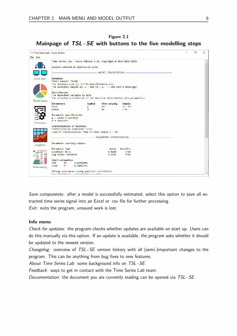
Figure 2.1Mainpage of TSL - SE with buttons to the five modelling steps

Save components: after a model is successfully estimated, select this option to save all ex-tracted time series signal into an Excel or .csv file for further processing.Exit: exits the program, unsaved work is lost.

Info menuCheck for updates: the program checks whether updates are available on start up. Users cando this manually via this option. If an update is available, the program asks whether it shouldbe updated to the newest version.Changelog : overview of TSL - SE version history with all (semi-)important changes to theprogram. This can be anything from bug fixes to new features.About Time Series Lab: some background info on TSL - SE .Feedback : ways to get in contact with the Time Series Lab team.Documentation: the document you are currently reading can be opened via TSL - SE .

Chapter 3

Step 1: Loading and preparing data

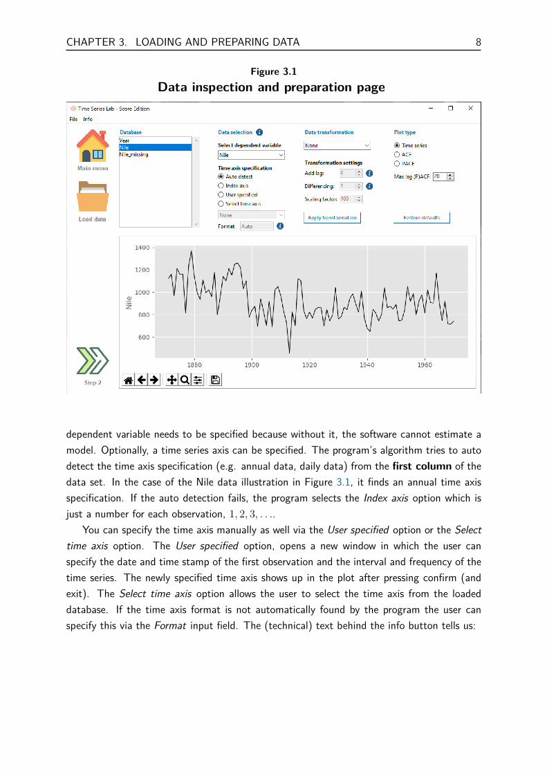
The first step in any time series analysis is the inspection and preparation ofdata. From the main page, clicking the button on the left brings you to the datainspection and preparation page as displayed in Figure 3.1. The Nile data set1 that

comes bundled with the installation file of TSL - SE is used as illustration.

3.1 DatabaseThe data set is loaded and selected from the file system by pressing the Load data button(below the Main menu button).

Important: The data set should be in column format with headers. The formatof the data should be *.xls(x), or *.csv, *.txt with comma’s as field separation.The program does not sort the data which means that the data should be in the

correct time series order before loading it into the program.

After loading the data, the headers of the data columns are displayed in the Database sectionat the top left of the page. Clicking on a header name plots the data in the plot area at thebottom of the page. As shown in 3.1, the Nile data is currently highlighted and (automati-cally) plotted.

3.2 Data selectionThe highlighted variable Nile also appears in the Select dependent variable pull down menu.This is the so-called y-variable of the time series equation and it is the time series variableof interest, i.e. the time series variable you want to model, analyze, and forecast. The

1The Nile data set consists of a series of readings of the annual flow volume of the river Nile at the cityof Aswan from 1871 to 1970.

CHAPTER 3. LOADING AND PREPARING DATA 8

Figure 3.1Data inspection and preparation page

dependent variable needs to be specified because without it, the software cannot estimate amodel. Optionally, a time series axis can be specified. The program’s algorithm tries to autodetect the time axis specification (e.g. annual data, daily data) from the first column of thedata set. In the case of the Nile data illustration in Figure 3.1, it finds an annual time axisspecification. If the auto detection fails, the program selects the Index axis option which isjust a number for each observation, 1, 2, 3, . . ..

You can specify the time axis manually as well via the User specified option or the Selecttime axis option. The User specified option, opens a new window in which the user canspecify the date and time stamp of the first observation and the interval and frequency of thetime series. The newly specified time axis shows up in the plot after pressing confirm (andexit). The Select time axis option allows the user to select the time axis from the loadeddatabase. If the time axis format is not automatically found by the program the user canspecify this via the Format input field. The (technical) text behind the info button tells us:

9 3.3. DATA TRANSFORMATION

Specify date format codes according to the 1989 C-standard convention, e.g.

2020-01-27: %Y-%m-%d2020(12): %Y(%m)2020/01/27 09:51:43: %Y/%m/%d %H:%M:%S

Specify ‘Auto’ for auto detection of the date format.

Note that a time axis is not strictly necessary for the program to run and an Index axis willalways do.

3.3 Data transformationIf needed, you can transform the data before modelling. For example if the time series con-sists of values of the Dow Jones Index, a series of percentage returns can be obtained byselecting percentage change from the Data transformation pull down menu followed by click-ing the Apply transformation button. Note that the (original) variable before transformationshould be highlighted before applying the transformation to tell the program which variableto transform. An example is given in Figure 3.2 where the Nile data is transformed by takinglogs. The newly transformed log variable (Nile log) is added to the variables in the Databasesection and is automatically highlighted and plotted after the transformation. Transforma-tions can be combined by applying transformations to already transformed variables. Newlycreated transformed variables can be removed from the database by right mouse clicking onit and selecting the Delete from database option. For the transformations: Lag operator,Difference, and Scaling, the program needs extra user input. Depending on the selection, spinboxes under Transformation settings become operable.

Add lag:Lagged variables can be added to the model as well. Often these are explanatory variables,e.g. Xt−1. Lagging a time series means shifting it in time. The number of periods shiftedcan be controlled by the Add lag spin box. Note the text behind the information buttons thatsays:

Please note that values > 0 are lags and values < 0 are leads

Differencing:A non-stationary time series2 can be made stationary by differencing. For example, if yt

2A stationary time series is one whose statistical properties such as mean and variance are constant overtime.

CHAPTER 3. LOADING AND PREPARING DATA 10

denotes the value of the time series at period t, then the first difference of yt at period t isequal to yt− yt−1, that is, we subtract the previous observation from the current observation.TSL - SE accommodates for this procedure since differencing is common practice among timeseries researchers. However, the methodology of TSL - SE allows the user to explicitly modelnon-stationary time series and differencing is not strictly necessary. Note the text behind theinformation buttons that tells us:

Time Series Lab allows the user to explicitly model non-stationary components like trend and seasonal.However, users might prefer to make the time series stationary by taking first / seasonal differencesbefore modelling.

Please note that missing values are added to the beginning of the sample to keep the timeseries length equal to the original time series length before the difference operation.

Scaling:Estimating a time series that consist of several or some small values, e.g. < 0.001, couldpotentially lead to numerical instabilities. This can be solved by scaling the time series tomore manageable numbers.

3.4 Graphical inspection of the dataPlot typeDifferent types of time series plots can be activated by selecting one of the three options:Time series, ACF, or PACF. The Time series option plots the selected time series. ACF andPACF plots are advanced time series features and the explanation and ideas behind them areout of the scope of this manual.

PlotsThe plot area at the bottom of the window has more option than shown here. For example,clicking the right mouse button on the plot area opens a menu with additional options. Thetitle of the plot, and the axes titles can be specified. Furthermore, characteristics of theselected time series can be plotted in the top right corner of the graph. Finally, the buttonsin the bottom left corner of the plot area add additional functionality such as zooming in andsaving of the figure to a drive.

It is time to go to step 2 of the modelling process. Please press the Step 2 button in theleft bottom corner of your screen to go to the Model setup page.

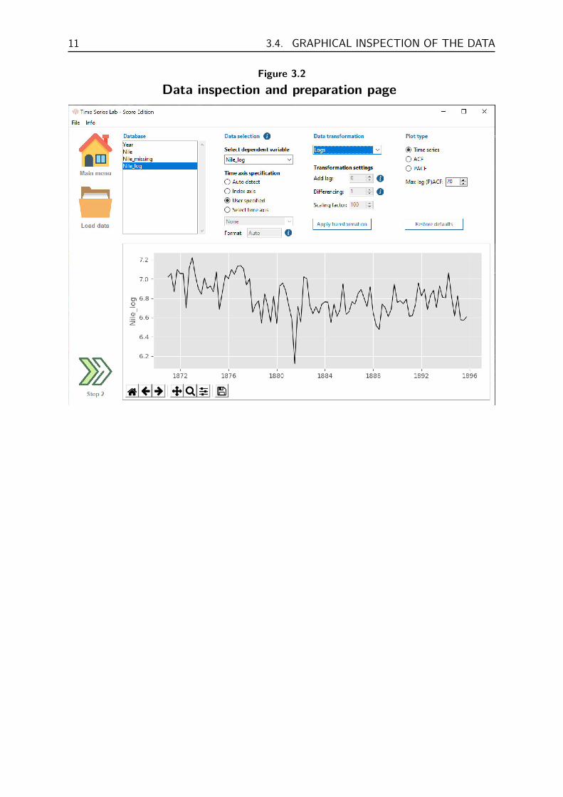
11 3.4. GRAPHICAL INSPECTION OF THE DATA

Figure 3.2Data inspection and preparation page

Chapter 4

Step 2: Model setup

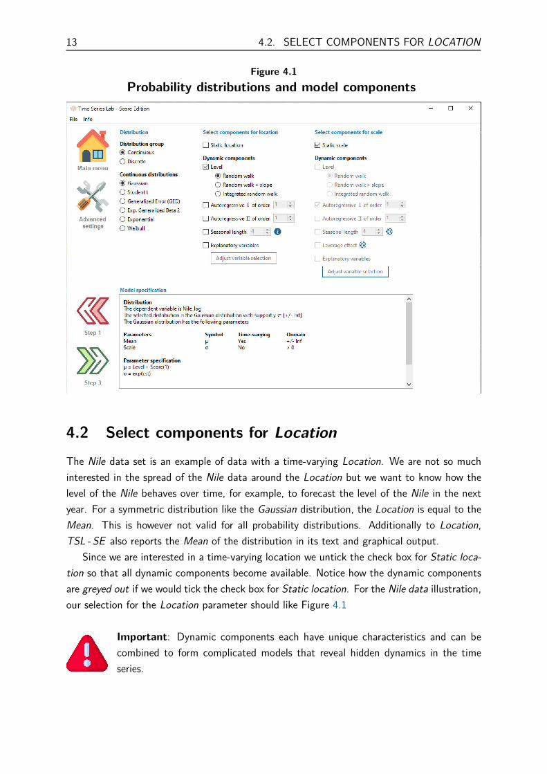
Step 2 of the software looks like Figure 4.1 and can be reached via the Main menu,or via Step 1 or Step 3. Step 2 is the heart of the program and it is here whereimportant modelling decision are made. The selections on this page are based on

what we want to model and what our data characteristics are.

Important: Always ask yourself, “Which parameter needs to be time-varying?”Is it the mean (location) of the distribution or the variance (scale). In TSL - SE itis even possible to have both parameters time-varying.

4.1 DistributionTSL - SE divides the probability distributions in two Distribution groups; Continuous dis-tributions and Discrete distributions. The choice of distribution depends strongly on thecharacteristics of the time series data. The Discrete distributions are the most specific ofthe two groups because they can only be applied to discrete data, in contrast to Continuousdistributions who can handle both continuous and discrete data. Discrete data can only takecertain values and are often integers (whole numbers) but categorical data could also be re-garded as discrete. Examples of discrete data are the number of goals scored by a footballteam or the number of earthquakes in a certain region. Continuous data are not restricted tocertain values, and can occupy any value over a continuous range. Examples of continuousdata are stock returns or the lap times of an F1 car.

From the choice of distributions, the Gaussian is the most well-known but it is not theonly one. And here lies the power of TSL - SE : the program can handle so many different timeseries because several probability distributions which each there own unique specifications arepart of TSL - SE . This makes the program extremely versatile and almost any time series canbe analyzed with the software.

We continue with the Nile data that we loaded in Step 1 and select the Gaussian distri-bution for our data, see Figure 4.1.

13 4.2. SELECT COMPONENTS FOR LOCATION

Figure 4.1Probability distributions and model components

4.2 Select components for LocationThe Nile data set is an example of data with a time-varying Location. We are not so muchinterested in the spread of the Nile data around the Location but we want to know how thelevel of the Nile behaves over time, for example, to forecast the level of the Nile in the nextyear. For a symmetric distribution like the Gaussian distribution, the Location is equal to theMean. This is however not valid for all probability distributions. Additionally to Location,TSL - SE also reports the Mean of the distribution in its text and graphical output.

Since we are interested in a time-varying location we untick the check box for Static loca-tion so that all dynamic components become available. Notice how the dynamic componentsare greyed out if we would tick the check box for Static location. For the Nile data illustration,our selection for the Location parameter should like Figure 4.1

Important: Dynamic components each have unique characteristics and can becombined to form complicated models that reveal hidden dynamics in the timeseries.

CHAPTER 4. MODEL SETUP 14

Intermezzo 1: Time-varying components

TSL - SE extracts a signal from the observed time series. The difference between theobserved time series and the signal is the noise, or the error. The methodology ofTSL - SE falls in the class of filters since it filters the time series from the noise toobtain signal. It is the signal what we are interested in because it tells us somethingabout the next time period. In its simplest form, the signal at time t is equal to itsvalue in t− 1 plus some innovation. In mathematical form we have

αt = αt−1 + some innovation,

with αt being the signal for t = 1, . . . , T where T is the length of the time series. Theinnovation part is what drives the signal over time. In the score-driven methodologyas explained in Appendix B, the scaled score of the predictive density is the driver. Amore advanced model can be constructed by combining components, for example

αt = µt + γt +Xtβ,

where µt is the level component, γt is the seasonal component, Xtβ are explanatoryvariables, and where each of the components have their own score updating function.

We discuss each dynamic component and its characteristics.

LevelThe Level component is a non-stationary component. In its simplest form it’s a Random walkand can be extended with a drift parameter for direction. The Integrated random walk is a spe-cial type of Random walk + drift component and often gives a smooth(er) pattern over time.Although the Random walk is mathematically very simple, it proves very useful in many cases.

Autoregressive I and IIThe Autoregressive component is a stationary component. Its order can be specified up tolags of p = 31. TSL - SE always restricts the autoregressive parameters in such a way thatthe autoregressive process stays within the stationary region.

SeasonalThe Seasonal component is a non-stationary component. Its seasonal length can be specifiedup to s = 52. The s seasonal components sum up to zero for identification. This is enforcedby estimating the first s− 1 which, together with the zero sum restriction, identifies the lastone (more in this in Step 3 of Section 5). The number of seasons of the Seasonal componentdepends on the data. Number of seasons should not be taken literally (although for quarterlydata it would be correct). It refers to the number of periods before the seasonal process

15 4.3. SELECT COMPONENTS FOR SCALE

repeats itself. The info button clarifies more and tells us:

Examples of seasonal specifications are:Monthly data, s = 12.Quarterly data, s = 4.Daily data, when modelling the weekly pattern, s = 7.

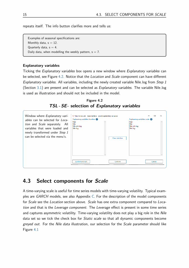
Explanatory variablesTicking the Explanatory variables box opens a new window where Explanatory variables canbe selected, see Figure 4.2. Notice that the Location and Scale component can have differentExplanatory variables. All variables, including the newly created variable Nile log from Step 1(Section 3.1) are present and can be selected as Explanatory variables. The variable Nile logis used as illustration and should not be included in the model.

Figure 4.2TSL - SE- selection of Explanatory variables

Window where Explanatory vari-ables can be selected for Loca-tion and Scale separately. Allvariables that were loaded andnewly transformed under Step 1can be selected via the menu’s.

4.3 Select components for ScaleA time-varying scale is useful for time series models with time-varying volatility. Typical exam-ples are GARCH models, see also Appendix C. For the description of the model componentsfor Scale see the Location section above. Scale has one extra component compared to Loca-tion and that is the Leverage component. The Leverage effect is present in some time seriesand captures asymmetric volatility. Time-varying volatility does not play a big role in the Niledata set so we tick the check box for Static scale so that all dynamic components becomegreyed out. For the Nile data illustration, our selection for the Scale parameter should likeFigure 4.1

CHAPTER 4. MODEL SETUP 16

4.4 Model specificationAt the bottom of our Step 2 screen, we find a summary of all our model decisions, seealso Figure 4.1. Our component selections and settings are directly translated to this modelsummary. The number of probability distribution parameters differ per distribution. Forexample the Poisson distribution only has one parameter (Location or Intensity) while theExp. Generalized Beta 2 distribution has four (Location, Scale, and two shape parameters).Only Location and Scale parameter can be selected as time-varying.

4.5 Advanced settingsThe Advanced settings button as shown here on the left gives us access to theadvanced model settings.

4.5.1 Score settings

For model stability reasons, Inverse Fisher scaling is the best option for the majority of models,see Appendix B for more information about score scaling. Multiple lags of the score updatingfunction can be included in the model. The number of score lags can be set individually forLocation and Scale. For the majority of time series models, lag 1 will be sufficient. ARCHmodels can be replicated by ticking the Set α = φ check box, see Appendix C for moreinformation.

4.5.2 Advanced settings location / scale

Dynamic components need to be initialized, i.e. they need to start from some specified value.If more than one dynamic component is selected, a choice need to be made which componentshould be initialized to avoid identification issues. The component that is initialized is free tostart from a value other than zero, based on the model setting Unconditional mean, Estimate,or Mean of data sample.

The Unconditional mean option can only be selected for the stationary Autoregressivecomponents I and II for the simple reason that non-stationary components do not have anUnconditional mean. The initialization can be estimated as well meaning the first element ofthe dynamic component will be part of the hyper parameter vector that will be estimated inStep 3, see Section 5. The last initialization method is to determine the initialization non-parametrically from the data. For our Nile data example this translates to taking the averageof the first 10 observations of the time series. The sample range can be set to a differentnumber as well. A sample range of 1 means that the initialization component starts from thefirst observation of the time series. All non-initialization components start from zero to avoididentification issues.

17 4.5. ADVANCED SETTINGS

The link function creates, as the name suggest, a link between the signal and the modelcomponents. A unit link means a one-to-one relationship between the signal and the modelcomponents. The exponential link function is often used to ensure positivity. For example theintensity of a Poisson distribution cannot be negative so modelling the intensity λt = exp(αt)with αt being the signal at time t ensures that λt will never be negative. Another example is thevariance (or standard error) of a distribution which cannot be negative and is therefore oftenmodelled in combination with the exponential link function. For our Nile data illustration, weuse the model settings as shown in Figure 4.3.

It is time to go to Step 3 of the modelling process. Please press the Step 3 button in theleft bottom corner of your screen to go to the Estimation page.

Figure 4.3Probability distributions and model components

Chapter 5

Step 3: Estimation

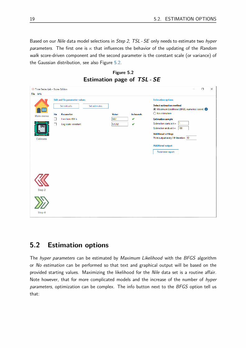
The estimation page of TSL - SE looks like Figure 5.2 and can be reached via theMain menu, or via Step 2 or Step 4. On this page we specify estimation settingsbased on the choices we made in Step 2.

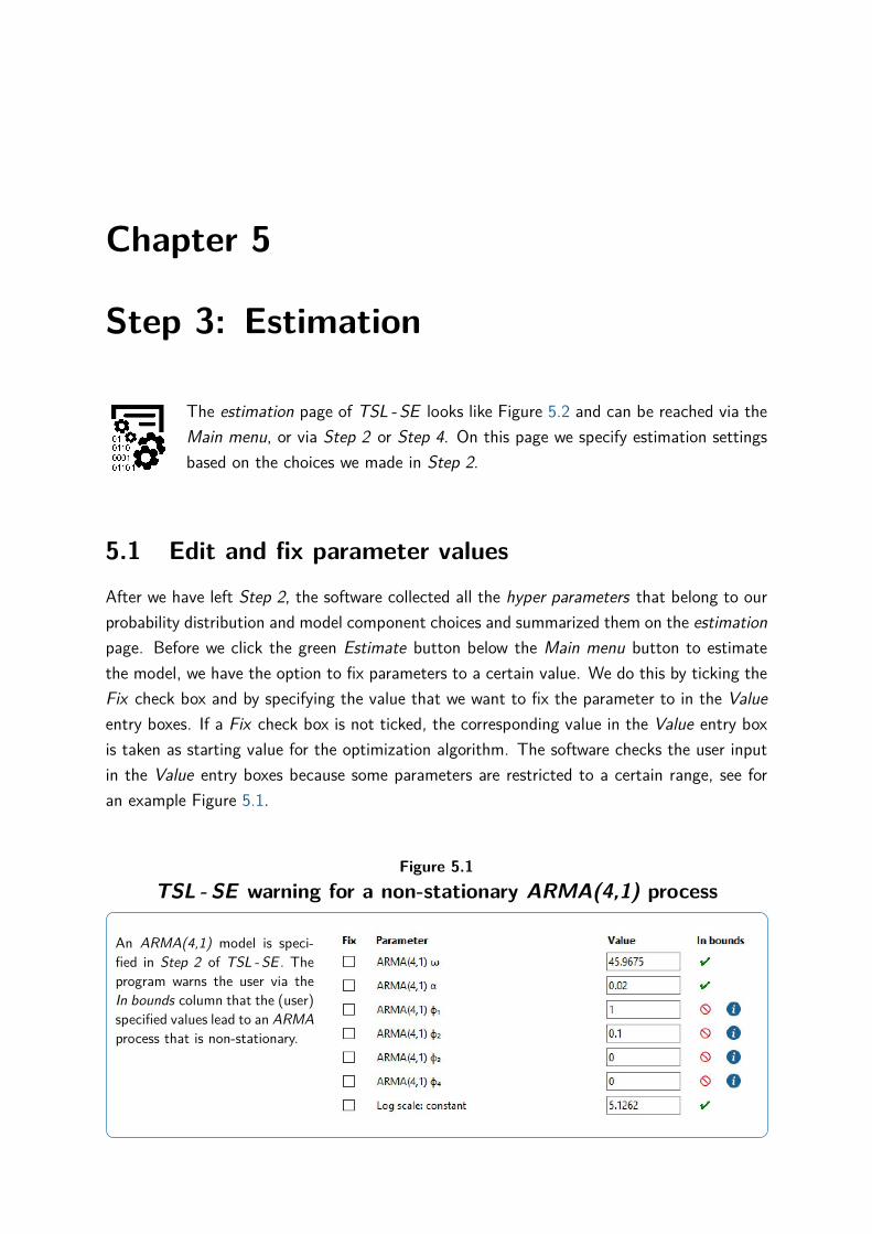
5.1 Edit and fix parameter valuesAfter we have left Step 2, the software collected all the hyper parameters that belong to ourprobability distribution and model component choices and summarized them on the estimationpage. Before we click the green Estimate button below the Main menu button to estimatethe model, we have the option to fix parameters to a certain value. We do this by ticking theFix check box and by specifying the value that we want to fix the parameter to in the Valueentry boxes. If a Fix check box is not ticked, the corresponding value in the Value entry boxis taken as starting value for the optimization algorithm. The software checks the user inputin the Value entry boxes because some parameters are restricted to a certain range, see foran example Figure 5.1.

Figure 5.1TSL - SE warning for a non-stationary ARMA(4,1) process

An ARMA(4,1) model is speci-fied in Step 2 of TSL - SE . Theprogram warns the user via theIn bounds column that the (user)specified values lead to an ARMAprocess that is non-stationary.

19 5.2. ESTIMATION OPTIONS

Based on our Nile data model selections in Step 2, TSL - SE only needs to estimate two hyperparameters. The first one is κ that influences the behavior of the updating of the Randomwalk score-driven component and the second parameter is the constant scale (or variance) ofthe Gaussian distribution, see also Figure 5.2.

Figure 5.2Estimation page of TSL - SE

5.2 Estimation optionsThe hyper parameters can be estimated by Maximum Likelihood with the BFGS algorithmor No estimation can be performed so that text and graphical output will be based on theprovided starting values. Maximizing the likelihood for the Nile data set is a routine affair.Note however, that for more complicated models and the increase of the number of hyperparameters, optimization can be complex. The info button next to the BFGS option tell usthat:

CHAPTER 5. ESTIMATION 20

The BFGS method falls in the category of quasi-Newton optimizers. This class of optimizers isapplicable to many optimization problems and is often used to maximize a likelihood function. Pleasebe aware that finding a global optimum is not guaranteed and trying different starting values increasesthe chance of finding the global optimum.

We are not restricted to estimating the full sample in our data set. If needed, we canrestrict the estimation to a more narrow sample by setting the Estimation starts at t andEstimation end at t entry boxes.

5.3 Additional outputAfter the successful estimation of a model, a (hyper) parameter report can be generated.Clicking the Parameter report button brings us to the Main page where the parameter reportwill be printed.

Important: The time it takes to generate the parameter report depends stronglyon the number of hyper parameters, the number of model components, and thelength of the time series. As a rule of thumb, the generation of a parameter report

takes at least the amount of time it takes to maximize the likelihood.

For our Nile data illustration, we use the model settings as shown in Figure 5.2. It is time togo to Step 4 of the modelling process. Please click the green Estimate button below the Mainmenu button to start the estimation process. During estimation we will see the Main pagewith (intermediate) optimization results and once the optimization is finished we will be takento the Graphical output of Step 4. During and after the estimation of the Nile model we seethe text output in the next section.

5.4 Text output for Nile data seriesTime Series Lab - Score Edition 1.20, Copyright c© 2019-2020 Nlitn

Session started at 2020-05-28 14:32

——————————————— MODEL DESCRIPTION ———————————————

DatabaseModel number: TSL001The database used is: C:/TSL/data/NileData.xlsxThe selection sample is: 1 - 100 (N = 1, T = 100 with 0 missings)

DistributionThe dependent variable is Nile

21 5.4. TEXT OUTPUT FOR NILE DATA SERIES

The selected distribution is the Gaussian distribution with parameters:

Parameters Symbol Time-varying DomainMean µ Yes +/- InfScale σ No > 0

Parameter specificationµ = Level + Score(1)σ = exp(cst)

Initialisation of locationInitialisation component: LevelType of initialisation: Mean of data sample 1 - 10

—————————————— PARAMETER OPTIMIZATION ——————————————

Parameter starting values:

Parameter type Value Free/FixLocation: RW κ 0.0200 FreeLog scale: constant 5.1262 Free

Start estimationit0 f= -6.64702486it10 f= -6.38052742

Strong convergence using numerical derivativesLog-likelihood = -638.052742; T = 100

Optimized parameter values:

Parameter type Value Free/FixLocation: RW κ 0.2483 FreeLog scale: constant 4.9616 Free

Estimation process completed in 0.0419 seconds

——————————————— STATE INFORMATION ———————————————

Component location Initial Time TMean 1132.6000 825.7410Random walk 1132.6000 825.7410

Component scale Initial Time TStandard deviation 142.8205 142.8205

Chapter 6

Step 4: Graphical output

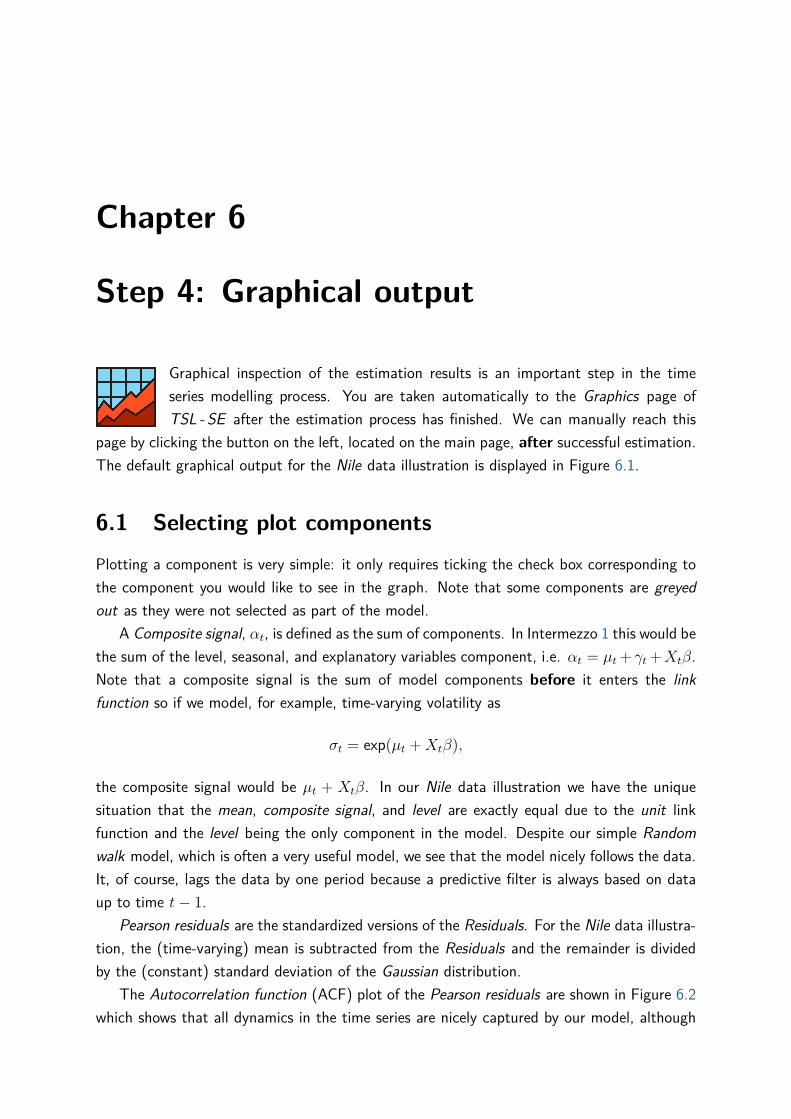
Graphical inspection of the estimation results is an important step in the timeseries modelling process. You are taken automatically to the Graphics page ofTSL - SE after the estimation process has finished. We can manually reach this

page by clicking the button on the left, located on the main page, after successful estimation.The default graphical output for the Nile data illustration is displayed in Figure 6.1.

6.1 Selecting plot componentsPlotting a component is very simple: it only requires ticking the check box corresponding tothe component you would like to see in the graph. Note that some components are greyedout as they were not selected as part of the model.

A Composite signal, αt, is defined as the sum of components. In Intermezzo 1 this would bethe sum of the level, seasonal, and explanatory variables component, i.e. αt = µt + γt +Xtβ.Note that a composite signal is the sum of model components before it enters the linkfunction so if we model, for example, time-varying volatility as

σt = exp(µt +Xtβ),

the composite signal would be µt + Xtβ. In our Nile data illustration we have the uniquesituation that the mean, composite signal, and level are exactly equal due to the unit linkfunction and the level being the only component in the model. Despite our simple Randomwalk model, which is often a very useful model, we see that the model nicely follows the data.It, of course, lags the data by one period because a predictive filter is always based on dataup to time t− 1.

Pearson residuals are the standardized versions of the Residuals. For the Nile data illustra-tion, the (time-varying) mean is subtracted from the Residuals and the remainder is dividedby the (constant) standard deviation of the Gaussian distribution.

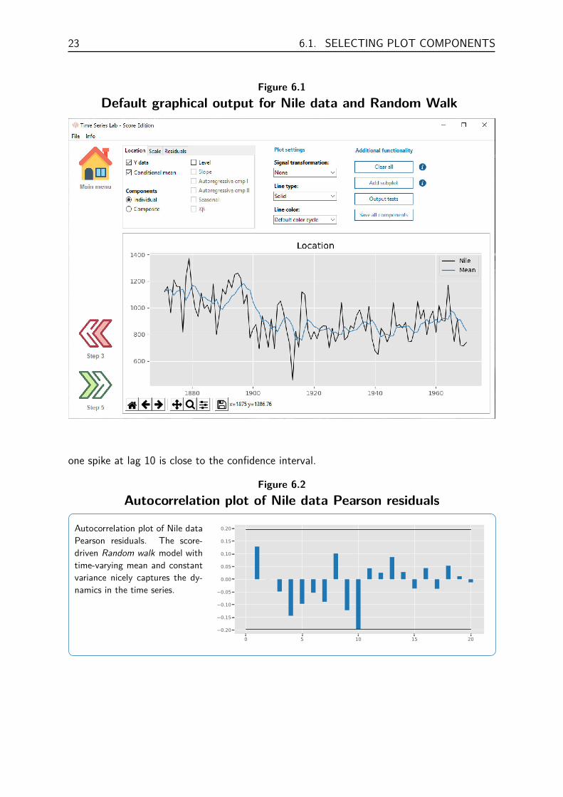
The Autocorrelation function (ACF) plot of the Pearson residuals are shown in Figure 6.2which shows that all dynamics in the time series are nicely captured by our model, although

23 6.1. SELECTING PLOT COMPONENTS

Figure 6.1Default graphical output for Nile data and Random Walk

one spike at lag 10 is close to the confidence interval.

Figure 6.2Autocorrelation plot of Nile data Pearson residuals

Autocorrelation plot of Nile dataPearson residuals. The score-driven Random walk model withtime-varying mean and constantvariance nicely captures the dy-namics in the time series.

0 5 10 15 200.20

0.15

0.10

0.05

0.00

0.05

0.10

0.15

0.20

CHAPTER 6. GRAPHICAL OUTPUT 24

6.2 Additional functionality

6.2.1 Clear all

The Clear all button is rigorous and clears everything from the graph including all subplots.To have more refined control over the (sub)plots, right-mouse click on a subplot for moreoptions. Section 6.2.2 discusses subplots in more detail.

6.2.2 Add subplot

The graph area of TSL - SE can consist of a maximum of nine subplots. Subplots can beconvenient to graphically summarize model results in one single plot. To add a subplot to thegraph, click the Add subplot button. Notice that an empty subplot is added to the existinggraph which correspond to no check boxes being ticked.

Important: The components that are graphically represented in a subplot directlycorrespond to the check boxes that are ticked. Clicking on a subplot activates thecurrent plot settings.

Notice that by clicking a subplot, a blue box appears shortly around the subplot as a sign thatthe subplot is active.

Location and scale components can be represented in one subplot, just activate the subplotof your choice and switch to the location or scale tab and tick the check boxes you need. Theinfo button to the right of the Add subplot button summarizes these findings and tells us:

Click on a subplot to activate it. Notice that by clicking on a subplot, the checkboxes in the top leftof the window change state based on the current selection of lines in the subplot.

If not all checkbox settings correspond with the lines in the subplot, switch the tabs to showthe rest of the selection.

6.2.3 Output tests

The residual Autocorrelation is graphically representation in the ACF plot. Autocorrelation canalso be tested by clicking the Output tests button. Durbin-Watson and Ljung-Box tests areperformed and output is printed to the Main page. Summary statistics of Residuals, PearsonResiduals, and Score are printed as well.

6.2.4 Save all components

All model components can be save to disc for further processing or archival purposes. Af-ter clicking the Save all components button, a window opens that allows you to save thecomponents to an *.xls(x) file or a comma separated *.csv file.

Chapter 7

Step 5: Forecasting

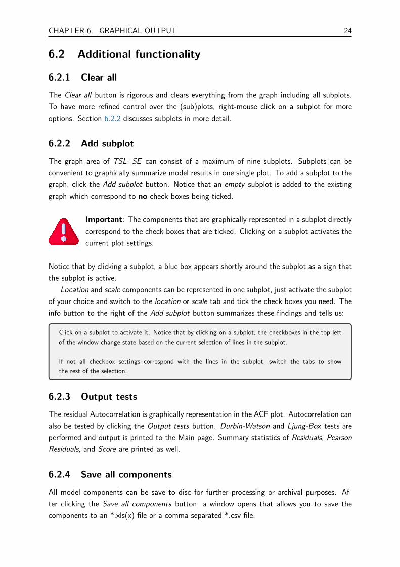
The forecasting page of TSL - SE with the Nile data as illustration looks likeFigure 7.1. The page can be reached via the Main menu or Step 4. Forecasting atime series if often of great interest for users because being able to say “something”

about the future can be of great value. Forecasts need to be evaluated in some way. This isusually done by loss functions which we will discuss later in this section.

7.1 Forecast settingsThe spin box located under forecast settings, currently has a reading of 10 and determines thenumber of time periods in the forecast window. The other spin box (with reading currently99) determines how many time points the program needs to plot before the first forecastperiod. Both spin boxes are interactive with the plot in the sense that changing them byclicking the up and down buttons immediately affect the plot window. Numbers can also beentered manually in the spin boxes followed by pressing the Enter key on the keyboard.

The current forecast selection can be cleared by clicking the Clear selection button andforecasts can be saved in *.xls(x) or *.csv format by clicking the Save all forecasts button.

7.2 Plot areaOur Nile data forecasts are show in Figure 7.1 for 10 time periods in the future. We see thatthe forecast is simply a straight line and no dynamics are present in the forecast. This is theresult of our model choices. We select a time-varying location composed of a score-drivenRandom walk component but the forecast of a Random walk is just the value of the lasttime period. Since we are out-of-sample with our forecasts (no observations are present), noscore-updating takes place and the result is a straight line into the future.

This is also the reason why the text box on the right of the graph only shows in-sampleloss functions because no observations are present after 1970 so losses cannot be calculated.Later in this section we will see an example where we do have out-of-sample observations. The

CHAPTER 7. FORECASTING 26

calculated loss functions are Root Mean Squared Error RMSE, Mean Absolute Error MAE,and Mean Absolute Percentage Error MAPE. The last one is not available for all data anddistribution combinations. The fourth value in the text box is the LogLoss which is defined asminus the average Log-likelihood value. Since many more loss functions are possible, forecastscan be saved with the Save all forecasts button to allow the user to apply tailor-made forecastthemselves.


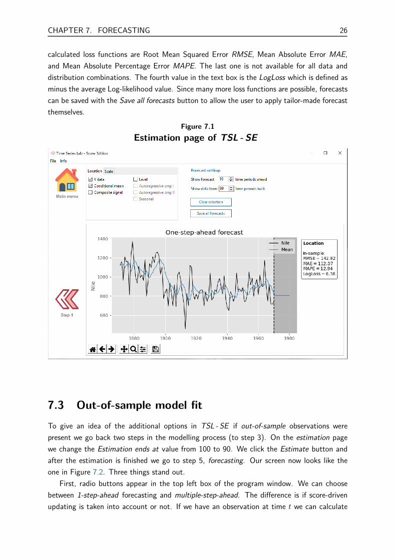
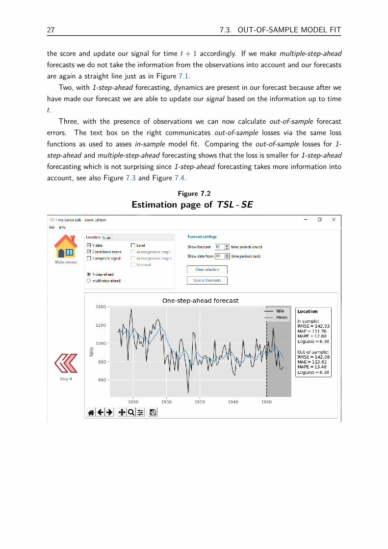
7.3 Out-of-sample model fitTo give an idea of the additional options in TSL - SE if out-of-sample observations werepresent we go back two steps in the modelling process (to step 3). On the estimation pagewe change the Estimation ends at value from 100 to 90. We click the Estimate button andafter the estimation is finished we go to step 5, forecasting. Our screen now looks like theone in Figure 7.2. Three things stand out.

First, radio buttons appear in the top left box of the program window. We can choosebetween 1-step-ahead forecasting and multiple-step-ahead. The difference is if score-drivenupdating is taken into account or not. If we have an observation at time t we can calculate

27 7.3. OUT-OF-SAMPLE MODEL FIT

the score and update our signal for time t + 1 accordingly. If we make multiple-step-aheadforecasts we do not take the information from the observations into account and our forecastsare again a straight line just as in Figure 7.1.

Two, with 1-step-ahead forecasting, dynamics are present in our forecast because after wehave made our forecast we are able to update our signal based on the information up to timet.

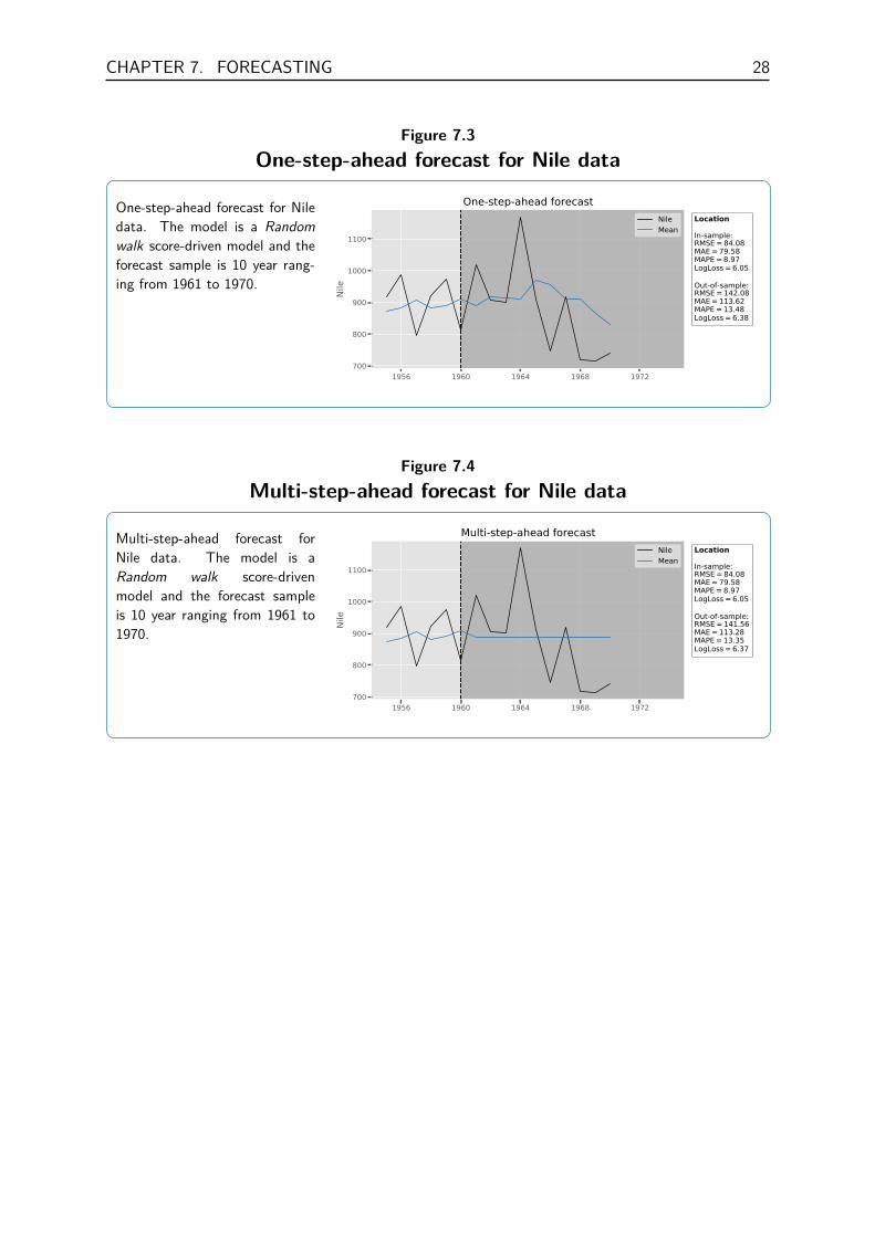
Three, with the presence of observations we can now calculate out-of-sample forecasterrors. The text box on the right communicates out-of-sample losses via the same lossfunctions as used to asses in-sample model fit. Comparing the out-of-sample losses for 1-step-ahead and multiple-step-ahead forecasting shows that the loss is smaller for 1-step-aheadforecasting which is not surprising since 1-step-ahead forecasting takes more information intoaccount, see also Figure 7.3 and Figure 7.4.


CHAPTER 7. FORECASTING 28

Figure 7.3One-step-ahead forecast for Nile data

One-step-ahead forecast for Niledata. The model is a Randomwalk score-driven model and theforecast sample is 10 year rang-ing from 1961 to 1970.

1956 1960 1964 1968 1972700

800

900

1000

1100

Nile

One-step-ahead forecastLocation

In-sample:RMSE = 84.08MAE = 79.58MAPE = 8.97LogLoss = 6.05

Out-of-sample:RMSE = 142.08MAE = 113.62MAPE = 13.48LogLoss = 6.38

NileMean

Figure 7.4Multi-step-ahead forecast for Nile data

Multi-step-ahead forecast forNile data. The model is aRandom walk score-drivenmodel and the forecast sampleis 10 year ranging from 1961 to1970.

1956 1960 1964 1968 1972700

800

900

1000

1100

Nile

Multi-step-ahead forecastLocation

In-sample:RMSE = 84.08MAE = 79.58MAPE = 8.97LogLoss = 6.05

Out-of-sample:RMSE = 141.56MAE = 113.28MAPE = 13.35LogLoss = 6.37

NileMean

Chapter 8

Case study

8.1 Estimating a dynamic Gompertz modelThis case study is based on the work by Harvey and Kattuman (2020) and Harvey and Lit(2020) and discusses the modelling of growth curves with an example in epidemiology andconcerns coronavirus. We fully replicate the modelling results and demonstrate the versatilityof TSL - SE . First a summary of the model

Intermezzo 2: dynamic growth curves model

The generalized logistic class of growth curves contains the logistic and Gompertz asspecial cases. They lead to a model in which the increase, yt, at time t depends on thecumulative total Yt. Specifically,

ln yt = ρ ln Yt−1 + δt + εt, ρ ≥ 1, t = 1, . . . , T, (8.1)

where yt = Yt−Yt−1, δt is a trend component, and εt is a serially independent Gaussiandisturbance with mean zero and constant variance, σ2

ε , that is εt ∼ NID(0, σ2ε).

When yt is small, it may be necessary to adopt a discrete distribution, particularlyif some observations are zero. A good choice is the negative binomial which, whenparameterized in terms of a time-varying mean, ξt, and a fixed positive shape parameter,υ, has probability mass function (PMF)

p(yt) = Γ(υ + yt)yt! Γ(υ) ξyt

t (υ + ξt)−yt(1 + ξt/υ)−υ, yt = 0, 1, 2, . . . .

An exponential link function ensures that ξt remains positive and at the same timeyields an equation similar to (8.1):

ln ξt = ρ ln Yt−1 + δt, t = 2, ..., T, (8.2)

CHAPTER 8. CASE STUDY 30

The model in Intermezzo 2 with ρ set to one is the dynamic Gompertz model and can be fullyreplicated in TSL - SE . We discuss all TSL - SE model settings step by step. The data usedin this case study is from March 11th 2020 up to, and including, May 6th was obtained fromthe ECDC website. The data comes bundled with the TSL - SE installer and the data file iscalled GermanyCovid.xlsx and is plotted in Figure A.1.

Front pageSelect the Score-driven models option in the Model category menu and click Get started.

Step 1Load the GermanyCovid.xlsx file located in the data folder of TSL - SE . Select the variableDGerDeath in the Database field or from the pull down menu under Select dependent variable.

Step 2Choose Discrete for the distribution group and Negative Binomial for the distribution. Makesure Static intensity is un-ticked. Tick the Level check box and select the Random walk+ slope component. Furthermore tick the Explanatory variables check box and select theLGerDeaths 1 explanatory variable for intensity. This variable is ln Yt−1 in Intermezzo 2.Make sure that the Autoregressive processes and the Seasonal are un-ticked.

Click the Advanced settings button and select the Estimate option under Type of initialisation.Choose the Exponential link function.

Step 3Fix the Log intensity: β LGerDeaths 1 parameter to 1.0 by ticking the Fix check box in frontof it and typing 1.0 in the Value field.Click the green Estimate button.

OutputWe should now see the graph in Figure A.2 on our screen and the following text output onthe main page.

Time Series Lab - Score Edition 1.20, Copyright c© 2019-2020 Nlitn



DatabaseModel number: TSL001The database used is: C:/TSL/data/GermanyCovid.xlsxThe selection sample is: 1 - 57 (N = 1, T = 57 with 0 missings)

Distribution

31 8.1. ESTIMATING A DYNAMIC GOMPERTZ MODEL

The dependent variable is DGerDeathThe selected distribution is the Negative Binomial distribution with parameters:

Parameters Symbol Time-varying DomainMean λ Yes > 0Dispersion r No > 0Parameter specificationλ = exp(Level + Xβ + Score(1))r = constant

Explanatory variablesExplanatory variable for location is: LGerDeaths 1

Initialisation of intensityInitialisation component: LevelType of initialisation: Estimate



Parameter type Value Free/FixLog intensity: RW κ 0.0200 FreeLog intensity: slope κ 0.0200 FreeLog intensity: init 4.8098 FreeLog intensity: init slope 0.0000 FreeLog intensity: β LGerDeaths 1 1.0000 FixedDispersion 5.0000 FreeStart estimationit0 f= -16.35430024it10 f= -5.43577140it20 f= -4.98910688it30 f= -4.91104728it40 f= -4.90077214it50 f= -4.89394127it60 f= -4.89272556it70 f= -4.89271867it80 f= -4.89271867it82 f= -4.89271867Strong convergence using numerical derivativesLog-likelihood = -278.884964; T = 57


Parameter type Value Free/FixLog intensity: RW κ 2.5372e-51 FreeLog intensity: slope κ 2.2026e-07 FreeLog intensity: init -0.2443 FreeLog intensity: init slope -0.0687 FreeLog intensity: β LGerDeaths 1 1.0000 FixedDispersion 5.7105 FreeEstimation process completed in 1.0981 seconds



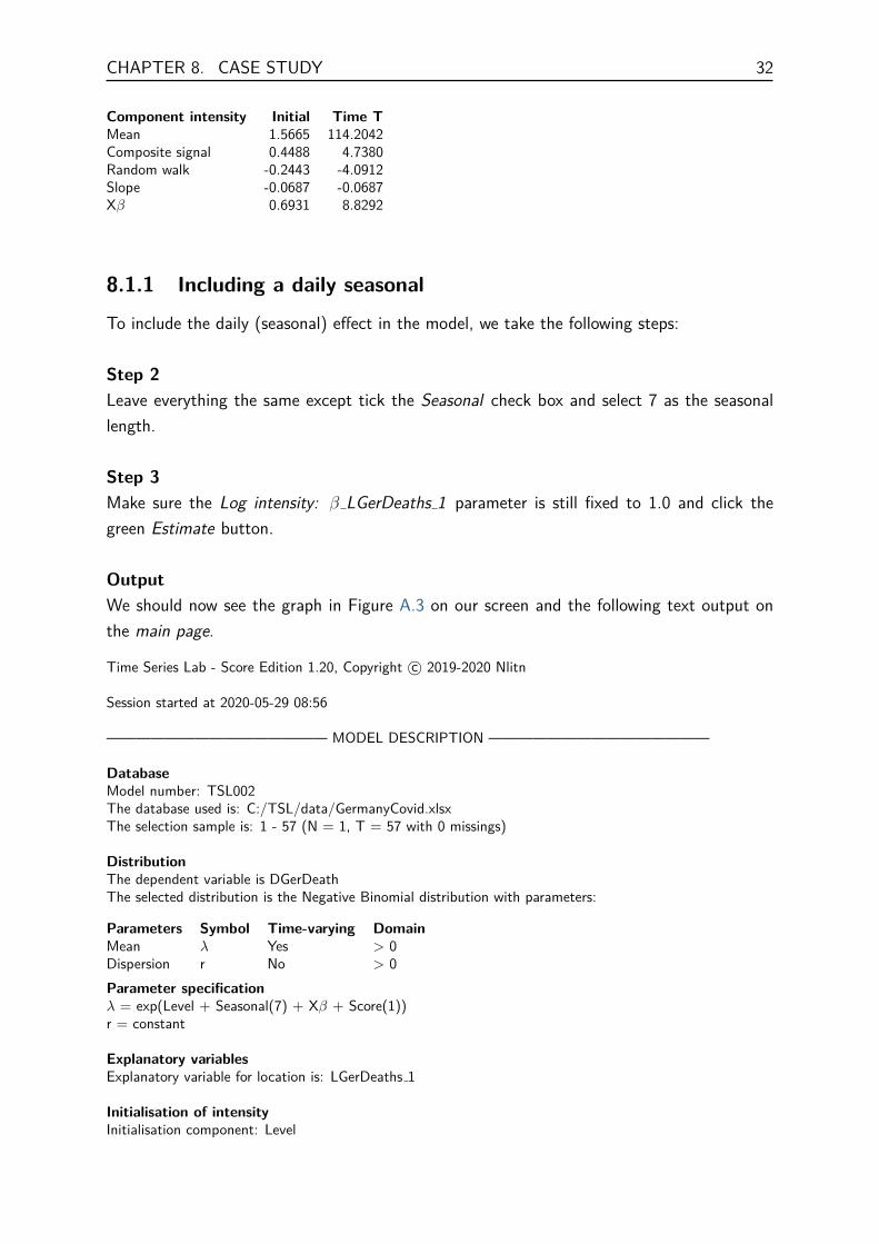
Component intensity Initial Time TMean 1.5665 114.2042Composite signal 0.4488 4.7380Random walk -0.2443 -4.0912Slope -0.0687 -0.0687Xβ 0.6931 8.8292

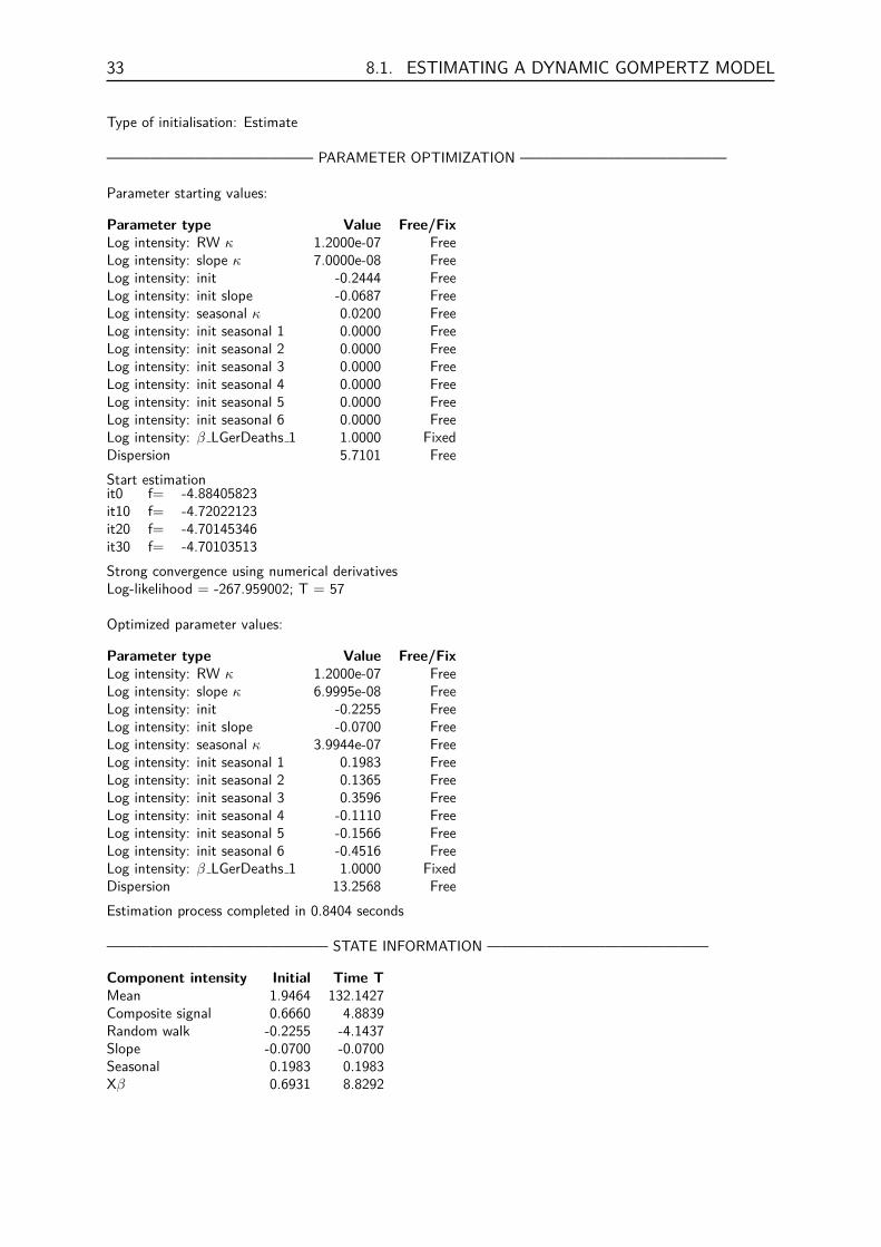
8.1.1 Including a daily seasonal

To include the daily (seasonal) effect in the model, we take the following steps:

Step 2Leave everything the same except tick the Seasonal check box and select 7 as the seasonallength.

Step 3Make sure the Log intensity: β LGerDeaths 1 parameter is still fixed to 1.0 and click thegreen Estimate button.

OutputWe should now see the graph in Figure A.3 on our screen and the following text output onthe main page.

Time Series Lab - Score Edition 1.20, Copyright c© 2019-2020 Nlitn



DatabaseModel number: TSL002The database used is: C:/TSL/data/GermanyCovid.xlsxThe selection sample is: 1 - 57 (N = 1, T = 57 with 0 missings)

DistributionThe dependent variable is DGerDeathThe selected distribution is the Negative Binomial distribution with parameters:

Parameters Symbol Time-varying DomainMean λ Yes > 0Dispersion r No > 0Parameter specificationλ = exp(Level + Seasonal(7) + Xβ + Score(1))r = constant

Explanatory variablesExplanatory variable for location is: LGerDeaths 1

Initialisation of intensityInitialisation component: Level

33 8.1. ESTIMATING A DYNAMIC GOMPERTZ MODEL

Type of initialisation: Estimate



Parameter type Value Free/FixLog intensity: RW κ 1.2000e-07 FreeLog intensity: slope κ 7.0000e-08 FreeLog intensity: init -0.2444 FreeLog intensity: init slope -0.0687 FreeLog intensity: seasonal κ 0.0200 FreeLog intensity: init seasonal 1 0.0000 FreeLog intensity: init seasonal 2 0.0000 FreeLog intensity: init seasonal 3 0.0000 FreeLog intensity: init seasonal 4 0.0000 FreeLog intensity: init seasonal 5 0.0000 FreeLog intensity: init seasonal 6 0.0000 FreeLog intensity: β LGerDeaths 1 1.0000 FixedDispersion 5.7101 FreeStart estimationit0 f= -4.88405823it10 f= -4.72022123it20 f= -4.70145346it30 f= -4.70103513Strong convergence using numerical derivativesLog-likelihood = -267.959002; T = 57


Parameter type Value Free/FixLog intensity: RW κ 1.2000e-07 FreeLog intensity: slope κ 6.9995e-08 FreeLog intensity: init -0.2255 FreeLog intensity: init slope -0.0700 FreeLog intensity: seasonal κ 3.9944e-07 FreeLog intensity: init seasonal 1 0.1983 FreeLog intensity: init seasonal 2 0.1365 FreeLog intensity: init seasonal 3 0.3596 FreeLog intensity: init seasonal 4 -0.1110 FreeLog intensity: init seasonal 5 -0.1566 FreeLog intensity: init seasonal 6 -0.4516 FreeLog intensity: β LGerDeaths 1 1.0000 FixedDispersion 13.2568 FreeEstimation process completed in 0.8404 seconds


Component intensity Initial Time TMean 1.9464 132.1427Composite signal 0.6660 4.8839Random walk -0.2255 -4.1437Slope -0.0700 -0.0700Seasonal 0.1983 0.1983Xβ 0.6931 8.8292


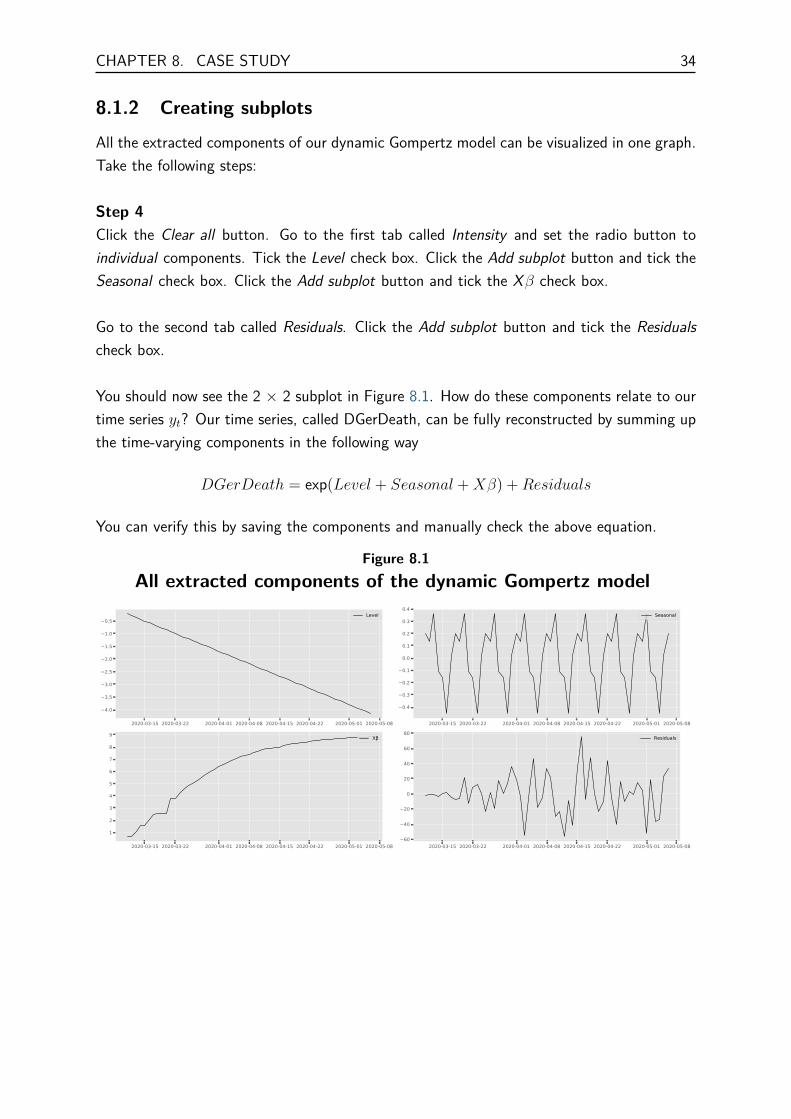
8.1.2 Creating subplots

All the extracted components of our dynamic Gompertz model can be visualized in one graph.Take the following steps:

Step 4Click the Clear all button. Go to the first tab called Intensity and set the radio button toindividual components. Tick the Level check box. Click the Add subplot button and tick theSeasonal check box. Click the Add subplot button and tick the Xβ check box.

Go to the second tab called Residuals. Click the Add subplot button and tick the Residualscheck box.

You should now see the 2 × 2 subplot in Figure 8.1. How do these components relate to ourtime series yt? Our time series, called DGerDeath, can be fully reconstructed by summing upthe time-varying components in the following way

DGerDeath = exp(Level + Seasonal +Xβ) +Residuals

You can verify this by saving the components and manually check the above equation.

Figure 8.1All extracted components of the dynamic Gompertz model

2020-03-15 2020-03-22 2020-04-01 2020-04-08 2020-04-15 2020-04-22 2020-05-01 2020-05-08

4.0

3.5

3.0

2.5

2.0

1.5

1.0

0.5Level

2020-03-15 2020-03-22 2020-04-01 2020-04-08 2020-04-15 2020-04-22 2020-05-01 2020-05-08

0.4

0.3

0.2

0.1

0.0

0.1

0.2

0.3

0.4Seasonal

2020-03-15 2020-03-22 2020-04-01 2020-04-08 2020-04-15 2020-04-22 2020-05-01 2020-05-08

1

2

3

4

5

6

7

8

9 X

2020-03-15 2020-03-22 2020-04-01 2020-04-08 2020-04-15 2020-04-22 2020-05-01 2020-05-0860

40

20

0

20

40

60

80Residuals

Appendices

Appendix A

Dynamic models

Why do we need dynamic models? Short answer, the world is dynamic. The more we cancapture dynamics, the better we understand the world’s processes and the better we canpredict them. Many processes exhibit some form of dynamic structure. The list of examplesis endless and contains almost every academic field. For example, finance where the volatilityof stock price returns is not constant over time. In Economics, where the sale of clothingitems exhibit strong seasonality due to summer and winter but also daily seasonal patternsbecause Saturday will be, in general, a more busy day than Monday, the trajectory of a rocketin Engineering, The El Nino effect due to change in water temperature in Climatology, thenumber of oak processionary caterpillars throughout the year in Biology, to name a diversefew. If we would be interested in saying anything meaningful about the examples above weneed to deal with time-varyingness in some sort of way.

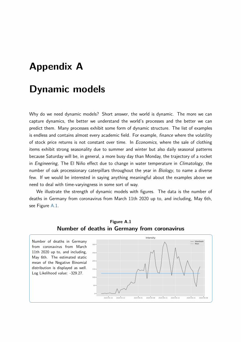
We illustrate the strength of dynamic models with figures. The data is the number ofdeaths in Germany from coronavirus from March 11th 2020 up to, and including, May 6th,see Figure A.1.

Figure A.1Number of deaths in Germany from coronavirus

Number of deaths in Germanyfrom coronavirus from March11th 2020 up to, and including,May 6th. The estimated staticmean of the Negative Binomialdistribution is displayed as well.Log Likelihood value: -329.27.

2020-03-15 2020-03-22 2020-04-01 2020-04-08 2020-04-15 2020-04-22 2020-05-01 2020-05-08

0

50

100

150

200

250

300

IntensityDGerDeathMean

37

The series is analysed by Harvey and Kattuman (2020) and Harvey and Lit (2020) with TSL -SE . Figure A.1 shows the static mean of the Negative Binomial distribution and we can clearlysee that a static mean would give a model fit that can be easily improved on. In the beginningof the sample the mean is much to high and during the worst period the static mean is farbelow the actual number of deaths. Needless to say, we could not use a static model to makeaccurate forecasts for this series. To capture the in-sample model fit in a number, we use theLog Likelihood value which for the Negative Binomial model and a static mean, applied tothese series, is -329.27.

Now consider the situation if we would make the mean time-varying by allowing it to havesome smooth pattern over time, we refer to the case study in Chapter 8 and Harvey and Lit(2020) for model details. The dynamic mean clearly follows the data much better and as aresult our Log Likelihood value increases (strongly) to -278.83.

Figure A.2Number of deaths from coronavirus and time-varying mean

Number of deaths in Germanyfrom coronavirus and the dy-namic mean of the Negative Bi-nomial distribution. Log Likeli-hood value: -278.83.

2020-03-15 2020-03-22 2020-04-01 2020-04-08 2020-04-15 2020-04-22 2020-05-01 2020-05-08

0

50

100

150

200

250

300


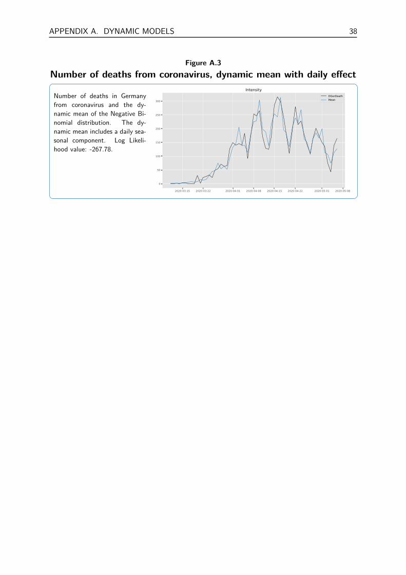
As it turns out, model fit can be further improved by taking into account the daily effect ofthe time series. The Log Likelihood value increases to -267.78 and the excellent model fit isdisplayed in Figure A.3. The figures in this section can all be replicated with TSL - SE , seethe case study in Chapter 8 for model details.

APPENDIX A. DYNAMIC MODELS 38

Figure A.3Number of deaths from coronavirus, dynamic mean with daily effect

Number of deaths in Germanyfrom coronavirus and the dy-namic mean of the Negative Bi-nomial distribution. The dy-namic mean includes a daily sea-sonal component. Log Likeli-hood value: -267.78.

2020-03-15 2020-03-22 2020-04-01 2020-04-08 2020-04-15 2020-04-22 2020-05-01 2020-05-08

0

50

100

150

200

250

300


Appendix B

Score-driven models

Consider a parametric model for an observed time series y = (y′1, . . . , y′n)′ that is formulatedconditionally on a latent m×1 time-varying parameter vector αt, for time index t = 1, . . . , n.We are interested in the statistical behavior of αt given a subset of the data, i.e. the dataup to time t − 1. One possible framework for such an analysis is the class of score-drivenmodels in which the latent time-varying parameter vector αt is updated over time using anautoregressive updating function based on the score of the conditional observation probabilitydensity function, see Creal et al. (2013) and Harvey (2013). The updating function for αt isgiven by

αt+1 = ω +p∑i=1

Aist−i+1 +q∑j=1

Bjαt−j+1,

where ω is a vector of constants, A and B are fixed coefficient matrices and st is the

scaled score function which is the driving force behind the updating equation. The unknowncoefficients ω, A and B depend on the static parameter vector ψ. The definition of st is

st = St · ∇t, ∇t = ∂ log p(yt|αt,Ft−1;ψ)∂αt

, t = 1, . . . , n,

where ∇t is the score vector of the (predictive) density p(yt|αt,Ft−1;ψ) of the observed time

series y = (y′1, . . . , y′n)′. The information set Ft−1 usually consists of lagged variables of αtand yt but can contain exogenous variables as well. To introduce further flexibility in themodel, the score vector ∇t can be scaled by a matrix St. Common choices for St are unitscaling, the inverse of the Fisher information matrix, or the square root of the Fisher inverseinformation matrix. The latter has the advantage of giving st a unit variance since the Fisherinformation matrix is the variance matrix of the score vector. In this framework and given pastinformation, the time-varying parameter vector αt is perfectly predictable one-step-ahead.

The score-driven model has three main advantages: (i) the ‘filtered’ estimates of the time-varying parameter are optimal in a Kullback-Leibler sense;(ii) since the score-driven modelsare observation driven, their likelihood is known in closed-form; and (iii) the forecasting per-

APPENDIX B. SCORE-DRIVEN MODELS 40

formance of these models is comparable to their parameter-driven counterparts, see Koopmanet al. (2016). The second point emphasizes that static parameters can be estimated in astraightforward way using maximum likelihood methods.

Appendix C

Submodels of score-driven models

Score-driven models encompass several other econometric models, among several well-knownlike ARMA models and the GARCH model of Engle (1982). Furthermore the ACD model ofEngle and Russell (1998), the autoregressive conditional multinomial (ACM) model of Russelland Engle (2005), the GARMA models of Benjamin et al. (2003), and the Poisson countmodels discussed by Davis et al. (2005). We now show mathematically how ARMA andGARCH models are submodels of score-driven models.

C.1 The ARMA modelConsider the time-varying mean model

yt = αt + εt, εt ∼ NID(0, σ2),

for t = 1, . . . , T and where NID means Normally Independently Distributed. If we apply thescore-driven methodology as discussed in Appendix B and we take p = q = 1 we have,

αt+1 = ω + βαt + κst, st = St · ∇,

where

∇t = ∂`t∂αt

, St = −Et−1

[∂2`t

∂αt∂αt

]−1

,

with`t = −1

2 log 2π − 12 logσ2 − 1

2σ2 (yt − αt)2.

We obtain∇t = 1

σ2 (yt − αt), St = σ2,

and st = yt − αt which is the prediction error. This means that the score updating becomes

αt+1 = ω + βαt + κ(yt − αt),

APPENDIX C. SUBMODELS OF SCORE-DRIVEN MODELS 42

and if we now replace αt = yt − εt, we have

yt+1 = ω + βyt + εt+1 + (κ− β)εt,

and hence score updating implies the ARMA(1,1) model for yt

yt = ω + φyt−1 + εt + θεt−1,

where φ ≡ β and θ = κ− β. Furthermore, if we set κ = β, we obtain the AR(1) model andif we set β = 0 we obtain the MA(1) model. The above is valid for higher lag orders p, q aswell which means that the score-driven framework encompasses the ARMA(p,q) model.

C.2 The GARCH modelThe strong results of the above section holds, with a couple of small changes, for the time-varying variance model as well. Consider the time-varying variance model

yt = µ+ εt, εt ∼ NID(0, αt),

for t = 1, . . . , T and where NID means Normally Independently Distributed. After settingµ = 0 we have the predictive logdensity

`t = −12 log 2π − 1

2 logαt −y2t

2αt.

We obtain∇t = 1

2α2t

y2t −

12αt

= 12α2

t

(y2t − αt).

Furthermore we have St = 2α2t and we obtain st = y2

t − αt. This means that the scoreupdating becomes

αt+1 = ω + βαt + κ(y2t − αt),

and hence score updating implies the GARCH(1,1) model

αt+1 = ω + φαt + κ∗y2t ,

where φ = β − κ and κ∗ ≡ κ. Furthermore, if we set κ = β, we obtain the ARCH(1) model.The above is valid for higher lag orders of p, q as well which means that the score-drivenframework encompasses the GARCH(p,q) model.

It should be emphasized that a score-driven time-varying variance model with Student tdistributed errors is not equal to a GARCH-t model.

Bibliography

Benjamin, M. A., R. A. Rigby, and D. M. Stasinopoulos (2003). Generalized autoregressivemoving average models. Journal of the American Statistical association 98(461), 214–223.

Creal, D. D., S. J. Koopman, and A. Lucas (2013). Generalized autoregressive score modelswith applications. Journal of Applied Econometrics 28(5), 777–795.

Davis, R. A., W. T. Dunsmuir, and S. B. Streett (2005). Maximum likelihood estimation foran observation driven model for poisson counts. Methodology and Computing in AppliedProbability 7(2), 149–159.

Engle, R. F. (1982). Autoregressive conditional heteroscedasticity with estimates of the vari-ance of united kingdom inflation. Econometrica 50(4), 987–1007.

Engle, R. F. and J. R. Russell (1998). Autoregressive conditional duration: a new model forirregularly spaced transaction data. Econometrica 66(5), 1127–1162.

Harvey, A. and R. Lit (2020). Coronavirus and the score-driven negative binomial distribution.Time Series Lab - Article Series (3).

Harvey, A. C. (2013). Dynamic Models for Volatility and Heavy Tails: With Applications toFinancial and Economic Time Series, Volume 52. Cambridge: Cambridge University Press.

Harvey, A. C. and P. Kattuman (2020). Time series models based on growth curves withapplications to forecasting coronavirus. Discussion paper, mimeo.

Koopman, S. J., A. Lucas, and M. Scharth (2016). Predicting time-varying parameters withparameter-driven and observation-driven models. Review of Economics and Statistics 98(1),97–110.

Russell, J. R. and R. F. Engle (2005). A discrete-state continuous-time model of financialtransactions prices and times: The autoregressive conditional multinomial–autoregressiveconditional duration model. Journal of Business & Economic Statistics 23(2), 166–180.

Time Series Lab - Article SeriesThe Time Series Lab - Article Series started in 2020 with Professor S.J. Koopman, Pro-fessor A.C. Harvey, and Dr. R.Lit as joint editors. The Time Series Lab - Article Series arededicated to research performed with Time Series Lab software. The scope of the seriesincludes the analysis and forecasting of a wide range of time series in fields like economics,finance, sports, climatology, biology, and health science. The following papers appeared inthe Time Series Lab - Article Series:

003 A.C. Harvey and R. Lit, Coronavirus and the Score-driven Negative Binomial Distribution

002 R. Lit and S.J Koopman, Forecasting the 2020 edition of the Boat Race

001 R. Lit, Forecasting the VIX in the midst of COVID-19

Documents

Time Series Lab Manual