Analyzing multinomial and time-series data

Dale J. Barr1 & Austin F. Frank2

1University of California, Riverside

2University of Rochester

WOMM, March 25, 2009

Our Goals

1. How to deal with a categorical response with > 2 categories

2. How to analyze time-series data with complex dependencies

A caveat before we begin

Estimation of models for multilevel multinomial data or fortime-series data are challenging problems individually; doing bothsimultaneously, even more so.

I a multinomial option is not implemented in many multilevelsoftware packages (e.g., lme4)

I time-series data can have complex dependencies that requirespecial techniques; approaches that use “regular” standarderrors without accounting for these dependencies are not tobe trusted!

To our knowledge there are no off-the-shelf software packages thatcan adequately do both. However, we have developed somesolutions, and at the end of the presentation we will give pointersto additional resources where people can get access to code andfind further information.

IntroductionMultinomial and time-series data

Paradigm example: Visual-world eyetracking data

Multilevel binomial logistic regressionModeling timeInterpreting results

Multilevel multinomial logistic regressionSpecifying the modelInterpreting the results

Appendix: Further info and resources

Multinomial data

It is often the case in observational and experimental research thatresponse variables are categorical, with more than two categories.

I Language production: Which linguistic category did aspeaker produce?

I Eyetracking: At which region is the subject looking at timet?

I Forced-choice experiments: To what phonemic categorydoes a stimulus belong?

Time-series data

Psycholinguistic studies are often interested in processes of changeover time:

I Language acquisition

I Perceptual learning / concept acquisition

I sentence processing research using event-related designs,such as mouse-tracking, eye-tracking, or ERP

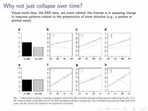
Why not just collapse over time?Visual-world data, like ERP data, are event related ; the interest is in assessing changein response patterns related to the presentation of some stimulus (e.g., a spoken orprinted word).

Paradigm case: Visual world eyetracking

QuestionDo people process language more efficiently when they haveprior knowledge that restricts the set of possible referents?

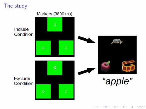
“apple”

I Listeners anticipate that the speaker willrefer to either:

I 1 of 2 (apple, chest);I 1 of 3 (apple, chest, turtle).

I Should need less speech info to select theapple in 2-referent than in 3-referentcondition

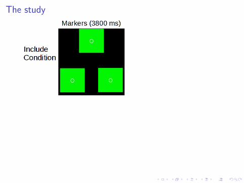
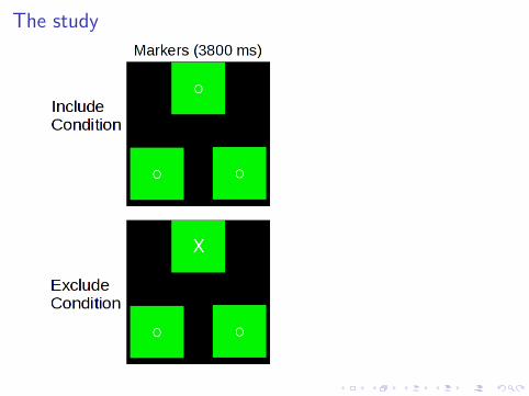
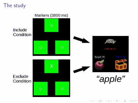
The study

The study

The study

The study

Data set

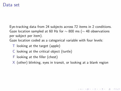
Eye-tracking data from 24 subjects across 72 items in 2 conditions.Gaze location sampled at 60 Hz for ∼ 800 ms (∼ 48 observationsper subject per item).Gaze location coded as a categorical variable with four levels:

T looking at the target (apple)

C looking at the critical object (turtle)

F looking at the filler (chest)

X (other) blinking, eyes in transit, or looking at a blank region

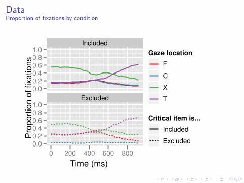
DataProportion of fixations by condition

Time (ms)

Pro

po

rtio

n o

f fixa

tio

ns

0.00.20.40.60.81.0

0.00.20.40.60.81.0

Included

Excluded

0 200 400 600 800

Gaze location

F

C

X

T

Critical item is...

Included

Excluded

Analysis 1: Multilevel binomial logistic regression

Approach:

I select a region (T,C,F) to analyze

I select a time window to perform the analysis

I test whether the proportion of fixations of that type changeswith time and condition within the window

Pros:

I Continuous time

I Performed in logit space

Cons:

I Only check one region at a time; can’t compare across regions

Analysis 1: Multilevel binomial logistic regression

Approach:

I select a region (T,C,F) to analyze

I select a time window to perform the analysis

I test whether the proportion of fixations of that type changeswith time and condition within the window

Pros:

I Continuous time

I Performed in logit space

Cons:

I Only check one region at a time; can’t compare across regions

Analysis 1: Multilevel binomial logistic regression

Approach:

I select a region (T,C,F) to analyze

I select a time window to perform the analysis

I test whether the proportion of fixations of that type changeswith time and condition within the window

Pros:

I Continuous time

I Performed in logit space

Cons:

I Only check one region at a time; can’t compare across regions

Analysis 1: Multilevel binomial logistic regression

Approach:

I select a region (T,C,F) to analyze

I select a time window to perform the analysis

I test whether the proportion of fixations of that type changeswith time and condition within the window

Pros:

I Continuous time

I Performed in logit space

Cons:

I Only check one region at a time; can’t compare across regions

Analysis 1: Multilevel binomial logistic regression

Approach:

I select a region (T,C,F) to analyze

I select a time window to perform the analysis

I test whether the proportion of fixations of that type changeswith time and condition within the window

Pros:

I Continuous time

I Performed in logit space

Cons:

I Only check one region at a time; can’t compare across regions

Analysis 1: Multilevel binomial logistic regression

Approach:

I select a region (T,C,F) to analyze

I select a time window to perform the analysis

I test whether the proportion of fixations of that type changeswith time and condition within the window

Pros:

I Continuous time

I Performed in logit space

Cons:

I Only check one region at a time; can’t compare across regions

Analysis 1: Multilevel binomial logistic regression

Approach:

I select a region (T,C,F) to analyze

I select a time window to perform the analysis

I test whether the proportion of fixations of that type changeswith time and condition within the window

Pros:

I Continuous time

I Performed in logit space

Cons:

I Only check one region at a time; can’t compare across regions

Analysis 1: Multilevel binomial logistic regression

Approach:

I select a region (T,C,F) to analyze

I select a time window to perform the analysis

I test whether the proportion of fixations of that type changeswith time and condition within the window

Pros:

I Continuous time

I Performed in logit space

Cons:

I Only check one region at a time; can’t compare across regions

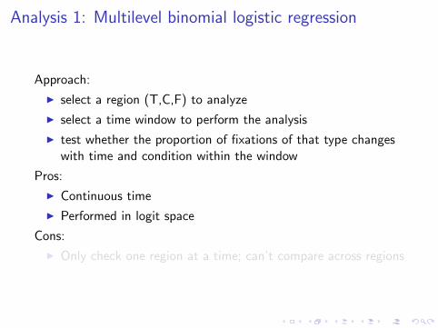
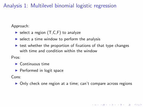
Analysis 1: Multilevel binomial logistic regression

Approach:

I select a region (T,C,F) to analyze

I select a time window to perform the analysis

I test whether the proportion of fixations of that type changeswith time and condition within the window

Pros:

I Continuous time

I Performed in logit space

Cons:

I Only check one region at a time; can’t compare across regions

Time as a continuous predictor

Time as a continuous predictor:

I For every unit change in time, make a change in the log oddsof the outcome that is a function of time

Possible functions inlude:

I Natural polynomials (Barr, 2008)

I Orthogonal polynomials (Mirman, Dixon, Magnuson, 2008)

I Splines

I Other nonlinear functions (Scheepers, Keller, Lapata, 2007)

Time as a continuous predictor

Time as a continuous predictor:

I For every unit change in time, make a change in the log oddsof the outcome that is a function of time

Possible functions inlude:

I Natural polynomials (Barr, 2008)

I Orthogonal polynomials (Mirman, Dixon, Magnuson, 2008)

I Splines

I Other nonlinear functions (Scheepers, Keller, Lapata, 2007)

Time as a continuous predictor

Time as a continuous predictor:

I For every unit change in time, make a change in the log oddsof the outcome that is a function of time

Possible functions inlude:

I Natural polynomials (Barr, 2008)

I Orthogonal polynomials (Mirman, Dixon, Magnuson, 2008)

I Splines

I Other nonlinear functions (Scheepers, Keller, Lapata, 2007)

Time as a continuous predictor

Time as a continuous predictor:

I For every unit change in time, make a change in the log oddsof the outcome that is a function of time

Possible functions inlude:

I Natural polynomials (Barr, 2008)

I Orthogonal polynomials (Mirman, Dixon, Magnuson, 2008)

I Splines

I Other nonlinear functions (Scheepers, Keller, Lapata, 2007)

Time as a continuous predictor

Time as a continuous predictor:

I For every unit change in time, make a change in the log oddsof the outcome that is a function of time

Possible functions inlude:

I Natural polynomials (Barr, 2008)

I Orthogonal polynomials (Mirman, Dixon, Magnuson, 2008)

I Splines

I Other nonlinear functions (Scheepers, Keller, Lapata, 2007)

Time as a continuous predictor

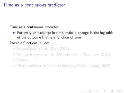
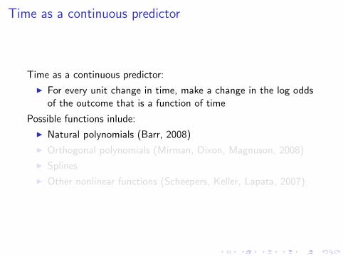
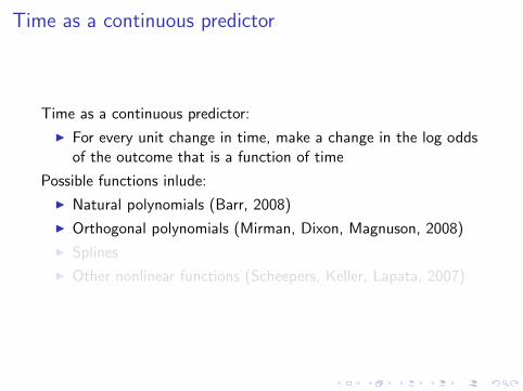
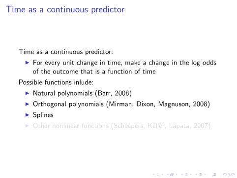
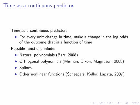
Time as a continuous predictor:

I For every unit change in time, make a change in the log oddsof the outcome that is a function of time

Possible functions inlude:

I Natural polynomials (Barr, 2008)

I Orthogonal polynomials (Mirman, Dixon, Magnuson, 2008)

I Splines

I Other nonlinear functions (Scheepers, Keller, Lapata, 2007)

Time as a continuous predictor

Time as a continuous predictor:

I For every unit change in time, make a change in the log oddsof the outcome that is a function of time

Possible functions inlude:

I Natural polynomials (Barr, 2008)

I Orthogonal polynomials (Mirman, Dixon, Magnuson, 2008)

I Splines

I Other nonlinear functions (Scheepers, Keller, Lapata, 2007)

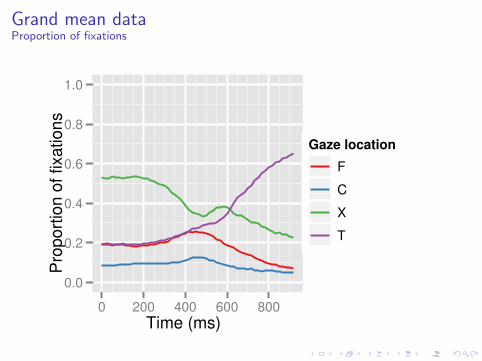
Grand mean dataProportion of fixations

Time (ms)

Pro

po

rtio

n o

f fixa

tio

ns

0.0

0.2

0.4

0.6

0.8

1.0

0 200 400 600 800

Gaze location

F

C

X

T

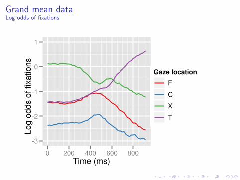
Grand mean dataLog odds of fixations

Time (ms)

Lo

g o

dd

s o

f fixa

tio

ns

-3

-2

-1

0

1

0 200 400 600 800

Gaze location

F

C

X

T

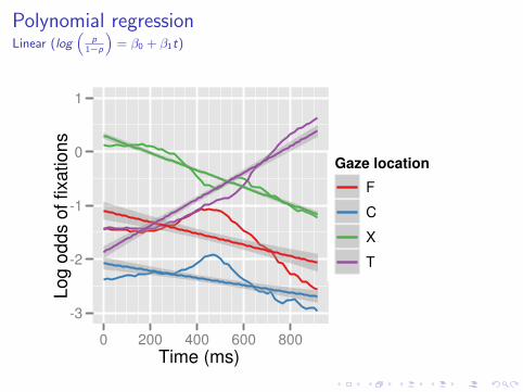
Polynomial regressionLinear (log

“p

1−p

”= β0 + β1t)

Time (ms)

Lo

g o

dd

s o

f fixa

tio

ns

-3

-2

-1

0

1

0 200 400 600 800

Gaze location

F

C

X

T

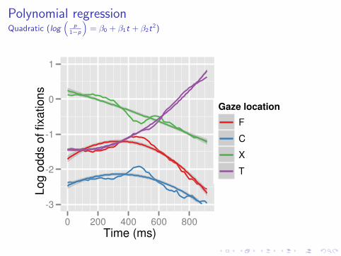
Polynomial regressionQuadratic (log

“p

1−p

”= β0 + β1t + β2t

2)

Time (ms)

Lo

g o

dd

s o

f fixa

tio

ns

-3

-2

-1

0

1

0 200 400 600 800

Gaze location

F

C

X

T

Polynomial regressionCubic (log

“p

1−p

”= β0 + β1t + β2t

2 + β3t2)

Time (ms)

Lo

g o

dd

s o

f fixa

tio

ns

-3

-2

-1

0

1

0 200 400 600 800

Gaze location

F

C

X

T

Polynomial regressionQuartic (log

“p

1−p

”= β0 + β1t + β2t

2 + β3t3 + β4t

4)

Time (ms)

Lo

g o

dd

s o

f fixa

tio

ns

-3

-2

-1

0

1

0 200 400 600 800

Gaze location

F

C

X

T

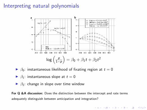
Interpreting natural polynomials

log(

p1−p

)= β0 + β1t + β2t

2

I β0: instantaneous likelihood of fixating region at t = 0

I β1: instantaneous slope at t = 0

I β2: change in slope over time window

For Q &A discussion: Does the distinction between the intercept and rate terms

adequately distinguish between anticipation and integration?

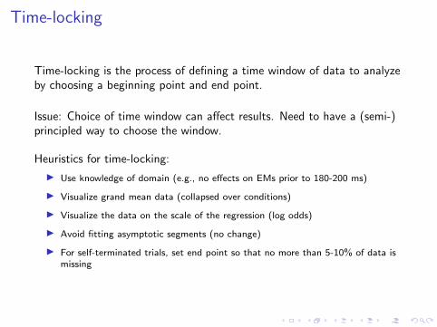
Time-locking

Time-locking is the process of defining a time window of data to analyzeby choosing a beginning point and end point.

Issue: Choice of time window can affect results. Need to have a (semi-)principled way to choose the window.

Heuristics for time-locking:

I Use knowledge of domain (e.g., no effects on EMs prior to 180-200 ms)

I Visualize grand mean data (collapsed over conditions)

I Visualize the data on the scale of the regression (log odds)

I Avoid fitting asymptotic segments (no change)

I For self-terminated trials, set end point so that no more than 5-10% of data ismissing

Time-locking

I Look for “breakpoint” tofind onset of stimulus-driveneffects

I Apparent breakpoint @ 200ms (NB: we will later seethat this break is unrelatedto referential processing)

I Choose end point based onRT (blue line representsprop. of trials that have notyet terminated)

I End point @ 783 ms (stillhave 95% of data)

Time-locking

I Look for “breakpoint” tofind onset of stimulus-driveneffects

I Apparent breakpoint @ 200ms (NB: we will later seethat this break is unrelatedto referential processing)

I Choose end point based onRT (blue line representsprop. of trials that have notyet terminated)

I End point @ 783 ms (stillhave 95% of data)

Time-locking

I Look for “breakpoint” tofind onset of stimulus-driveneffects

I Apparent breakpoint @ 200ms (NB: we will later seethat this break is unrelatedto referential processing)

I Choose end point based onRT (blue line representsprop. of trials that have notyet terminated)

I End point @ 783 ms (stillhave 95% of data)

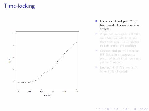
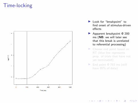
Time-locking

I Look for “breakpoint” tofind onset of stimulus-driveneffects

I Apparent breakpoint @ 200ms (NB: we will later seethat this break is unrelatedto referential processing)

I Choose end point based onRT (blue line representsprop. of trials that have notyet terminated)

I End point @ 783 ms (stillhave 95% of data)

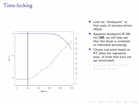
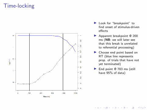
Choosing a polynomial function

Strategy:

I Use grand mean data so that model choice is not influencedby condition differences

I Visualize on the scale of the regression (log odds), log( p1−p ).

I Order of function is equal to number of bends + 1.

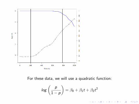
For these data, we will use a quadratic function:

log

(p

1− p

)= β0 + β1t + β2t

2

Parameterizing the model (fixed effects)

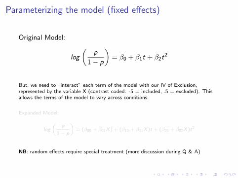
Original Model:

log

(p

1− p

)= β0 + β1t + β2t

2

But, we need to “interact” each term of the model with our IV of Exclusion,represented by the variable X (contrast coded: -5 = included, .5 = excluded). Thisallows the terms of the model to vary across conditions.

Expanded Model:

log

„p

1− p

«= (β00 + β01X ) + (β10 + β11X )t + (β20 + β02X )t2

NB: random effects require special treatment (more discussion during Q & A)

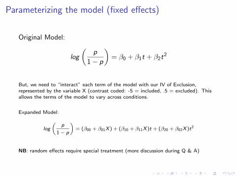
Parameterizing the model (fixed effects)

Original Model:

log

(p

1− p

)= β0 + β1t + β2t

2

But, we need to “interact” each term of the model with our IV of Exclusion,represented by the variable X (contrast coded: -5 = included, .5 = excluded). Thisallows the terms of the model to vary across conditions.

Expanded Model:

log

„p

1− p

«= (β00 + β01X ) + (β10 + β11X )t + (β20 + β02X )t2

NB: random effects require special treatment (more discussion during Q & A)

Results

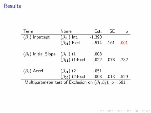
Term Name Est. SE p

(β0) Intercept (β00) Int. -1.390(β01) Excl -.514 .161 .001

(β1) Initial Slope (β10) t1 .008(β11) t1:Excl -.022 .078 .782

(β2) Accel. (β21) t2 .051(β22) t2:Excl .008 .013 .529

Multiparameter test of Exclusion on (β1,β2): p=.561.

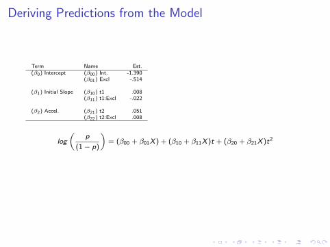
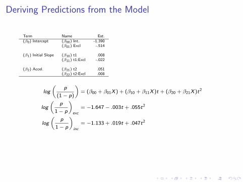
Deriving Predictions from the Model

Term Name Est.(β0) Intercept (β00) Int. -1.390

(β01) Excl -.514

(β1) Initial Slope (β10) t1 .008(β11) t1:Excl -.022

(β2) Accel. (β21) t2 .051(β22) t2:Excl .008

log

„p

(1− p)

«= (β00 + β01X ) + (β10 + β11X )t + (β20 + β21X )t2

Deriving Predictions from the Model

Term Name Est.(β0) Intercept (β00) Int. -1.390

(β01) Excl -.514

(β1) Initial Slope (β10) t1 .008(β11) t1:Excl -.022

(β2) Accel. (β21) t2 .051(β22) t2:Excl .008

log

„p

(1− p)

«= (β00 + β01X ) + (β10 + β11X )t + (β20 + β21X )t2

log

„p

(1− p)

«exc

= [−1.390 + .5(−.514)] + [.008 + .5(−.022)]t + [.051 + .5(.008)]t2

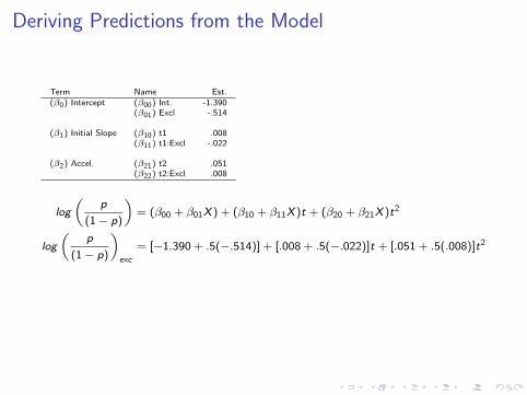
Deriving Predictions from the Model

Term Name Est.(β0) Intercept (β00) Int. -1.390

(β01) Excl -.514

(β1) Initial Slope (β10) t1 .008(β11) t1:Excl -.022

(β2) Accel. (β21) t2 .051(β22) t2:Excl .008

log

„p

(1− p)

«= (β00 + β01X ) + (β10 + β11X )t + (β20 + β21X )t2

log

„p

(1− p)

«exc

= [−1.390 + .5(−.514)] + [.008 + .5(−.022)]t + [.051 + .5(.008)]t2

= −1.647− .003t + .055t2

Deriving Predictions from the Model

Term Name Est.(β0) Intercept (β00) Int. -1.390

(β01) Excl -.514

(β1) Initial Slope (β10) t1 .008(β11) t1:Excl -.022

(β2) Accel. (β21) t2 .051(β22) t2:Excl .008

log

„p

(1− p)

«= (β00 + β01X ) + (β10 + β11X )t + (β20 + β21X )t2

log

„p

1− p

«exc

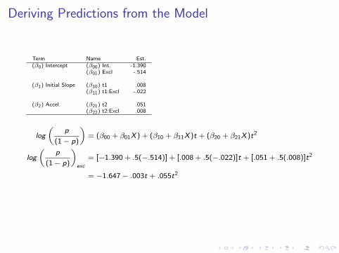
= −1.647− .003t + .055t2

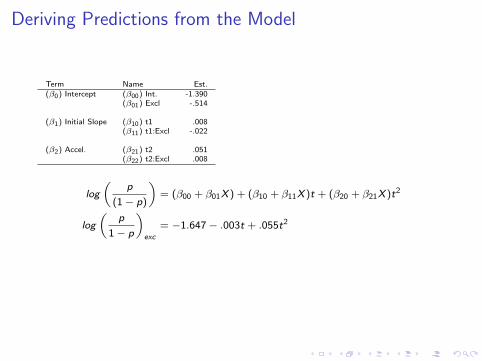
Deriving Predictions from the Model

Term Name Est.(β0) Intercept (β00) Int. -1.390

(β01) Excl -.514

(β1) Initial Slope (β10) t1 .008(β11) t1:Excl -.022

(β2) Accel. (β21) t2 .051(β22) t2:Excl .008

log

„p

(1− p)

«= (β00 + β01X ) + (β10 + β11X )t + (β20 + β21X )t2

log

„p

1− p

«exc

= −1.647− .003t + .055t2

log

„p

1− p

«inc

= −1.133 + .019t + .047t2

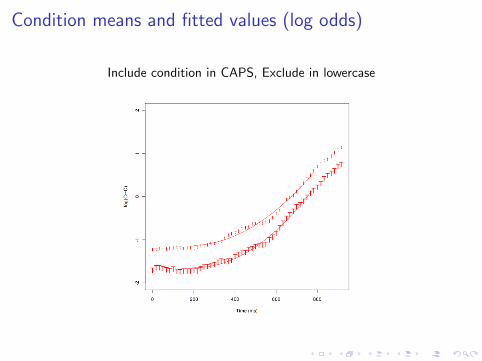
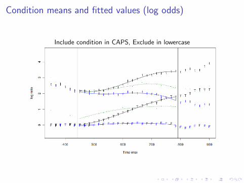
Condition means and fitted values (log odds)

Include condition in CAPS, Exclude in lowercase

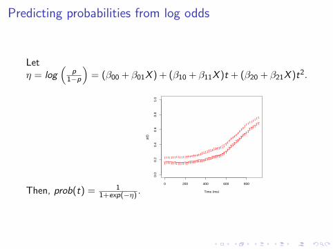
Predicting probabilities from log odds

Letη = log

(p

1−p

)= (β00 + β01X ) + (β10 + β11X )t + (β20 + β21X )t2.

Then, prob(t) = 11+exp(−η) .

TTTTTTTTTTTTTTTTTTTTTTTTTTTTTTTTTTTTTTTTTTTTTTTTTTTTTTTT

0 200 400 600 800

0.0

0.2

0.4

0.6

0.8

1.0

Time (ms)

p(t)

t t t t t t t t t t t t t t t t t t t t t t t t t t t t t t t t t t t t t ttt t t t t t

t tt t t t t t t t t

Multinomial Analysis

Polytomous response variables

Note that a subject’s current response at any given frame of eye data canbe classified into any of the following four exhaustive categories:

T looking at the target (apple)

C looking at the critical object (turtle)

F looking at the filler (chest)

X (other) blinking, eyes in transit, or looking at a blank region

The response variable is “polytomous” (having > 2 categories). Thecategories are exhaustive, so the probability that the subject is in any oneof the four states is 1. The categories are also mutually exclusive.

Binomial regression only allows us to model one of these states versus all

others—we have to dichotomize the variable—so the information it

provides is limited.

Baseline-category multinomial regression

The log ratio used in binomial regression compares a singleresponse to all others combined; e.g., log

(T¬T

)(target to “not

target”).

Using baseline-category multinomial regression, we can comparelooks at a given region to some “baseline” region. Because theprobabilities have to sum to 1, our four response categories can bemodeled by (4− 1) = 3 log ratios.

Note that visual-world eyetracking researchers often implement thisusing a “target advantage” score or by including region as avariable in the analysis. Both approaches have problems (topic forQ&A).

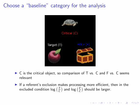
Choose a “baseline” category for the analysis

I C is the critical object, so comparison of T vs. C and F vs. C seemsrelevant

I If a referent’s exclusion makes processing more efficient, then in theexcluded condition log

(TC

)and log

(FC

)should be larger.

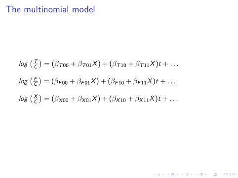
The multinomial model

log(

TC

)= (βT00 + βT01X ) + (βT10 + βT11X )t + . . .

log(

FC

)= (βF00 + βF01X ) + (βF10 + βF11X )t + . . .

log(

XC

)= (βX00 + βX01X ) + (βX10 + βX11X )t + . . .

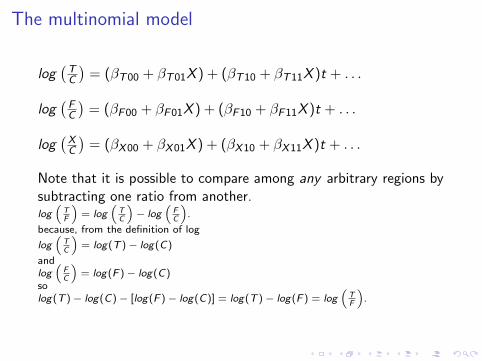
The multinomial model

log(

TC

)= (βT00 + βT01X ) + (βT10 + βT11X )t + . . .

log(

FC

)= (βF00 + βF01X ) + (βF10 + βF11X )t + . . .

log(

XC

)= (βX00 + βX01X ) + (βX10 + βX11X )t + . . .

Note that it is possible to compare among any arbitrary regions bysubtracting one ratio from another.log

“TF

”= log

“TC

”− log

“FC

”.

because, from the definition of log

log“

TC

”= log(T )− log(C)

andlog

“FC

”= log(F )− log(C)

solog(T )− log(C)− [log(F )− log(C)] = log(T )− log(F ) = log

“TF

”.

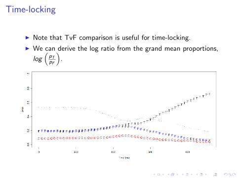
Time-locking

I Note that TvF comparison is useful for time-locking.

I We can derive the log ratio from the grand mean proportions,

log(

pTpF

).

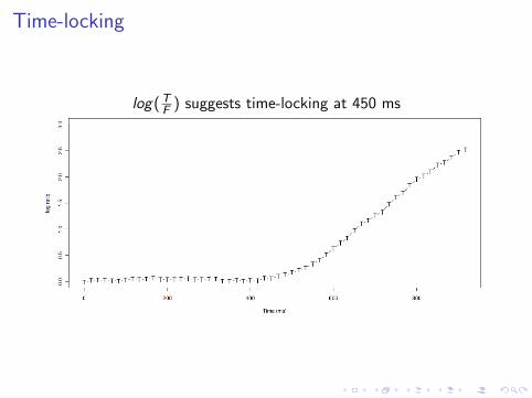
Time-locking

log(TF ) suggests time-locking at 450 ms

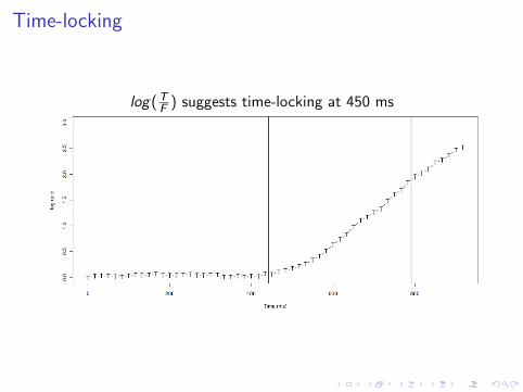
Time-locking

log(TF ) suggests time-locking at 450 ms

Choosing a polynomial function

Model choice heuristics:

I Use grand mean data so that model choice is not influencedby condition differences

I Visualize on the scale of the regression (log odds)

I Plot the relevant log ratios, log(TC ), log(F

C ), log(XC ).

I Order of function should be sufficient to capture mostcomplex curve.

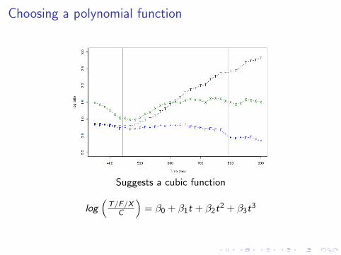
Choosing a polynomial function

Suggests a cubic function

log(

T/F/XC

)= β0 + β1t + β2t

2 + β3t3

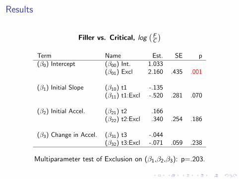
Results

Filler vs. Critical, log(

FC

)Term Name Est. SE p(β0) Intercept (β00) Int. 1.033

(β01) Excl 2.160 .435 .001

(β1) Initial Slope (β10) t1 -.135(β11) t1:Excl -.520 .281 .070

(β2) Initial Accel. (β21) t2 .166(β22) t2:Excl .340 .254 .186

(β3) Change in Accel. (β31) t3 -.044(β32) t3:Excl -.071 .059 .238

Multiparameter test of Exclusion on (β1,β2,β3): p=.203.

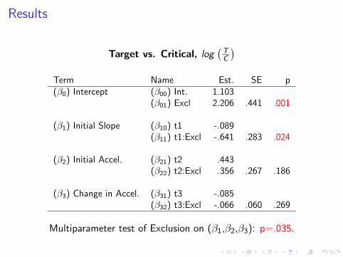
Results

Target vs. Critical, log(

TC

)Term Name Est. SE p(β0) Intercept (β00) Int. 1.103

(β01) Excl 2.206 .441 .001

(β1) Initial Slope (β10) t1 -.089(β11) t1:Excl -.641 .283 .024

(β2) Initial Accel. (β21) t2 .443(β22) t2:Excl .356 .267 .186

(β3) Change in Accel. (β31) t3 -.085(β32) t3:Excl -.066 .060 .269

Multiparameter test of Exclusion on (β1,β2,β3): p=.035.

Deriving Predictions from the Model

Term Name Est.(β0) Intercept (β00) Int. 1.033

(β01) Excl 2.160

(β1) Initial Slope (β10) t1 -.135(β11) t1:Excl -.520

(β2) Initial Accel. (β21) t2 .166(β22) t2:Excl .340

(β3) Change in Accel. (β31) t3 -.044(β32) t3:Excl -.071

log

„F

C

«= (β00 + β01X ) + (β10 + β11X )t + (β20 + β21X )t2 + (β30 + β31X )t3

Deriving Predictions from the Model

Term Name Est.(β0) Intercept (β00) Int. 1.033

(β01) Excl 2.160

(β1) Initial Slope (β10) t1 -.135(β11) t1:Excl -.520

(β2) Initial Accel. (β21) t2 .166(β22) t2:Excl .340

(β3) Change in Accel. (β31) t3 -.044(β32) t3:Excl -.071

log

„F

C

«= (β00 + β01X ) + (β10 + β11X )t + (β20 + β21X )t2 + (β30 + β31X )t3

log

„F

C

«exc

= [1.033 + .5(2.160)] + [−.135 + .5(−.520)]t+

[.166 + .5(.340)]t2 + [−.044 + .5(−.071)]t3

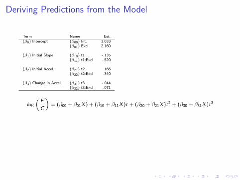
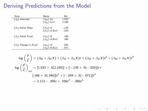
Deriving Predictions from the Model

Term Name Est.(β0) Intercept (β00) Int. 1.033

(β01) Excl 2.160

(β1) Initial Slope (β10) t1 -.135(β11) t1:Excl -.520

(β2) Initial Accel. (β21) t2 .166(β22) t2:Excl .340

(β3) Change in Accel. (β31) t3 -.044(β32) t3:Excl -.071

log

„F

C

«= (β00 + β01X ) + (β10 + β11X )t + (β20 + β21X )t2 + (β30 + β31X )t3

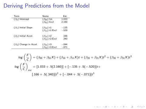
log

„F

C

«exc

= [1.033 + .5(2.160)] + [−.135 + .5(−.520)]t+

[.166 + .5(.340)]t2 + [−.044 + .5(−.071)]t3

= 2.113− .395t + .336t2 − .080t3

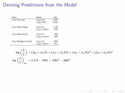
Deriving Predictions from the Model

Term Name Est.(β0) Intercept (β00) Int. 1.033

(β01) Excl 2.160

(β1) Initial Slope (β10) t1 -.135(β11) t1:Excl -.520

(β2) Initial Accel. (β21) t2 .166(β22) t2:Excl .340

(β3) Change in Accel. (β31) t3 -.044(β32) t3:Excl -.071

log

„F

C

«= (β00 + β01X ) + (β10 + β11X )t + (β20 + β21X )t2 + (β30 + β31X )t3

log

„F

C

«exc

= 2.113− .395t + .336t2 − .080t3

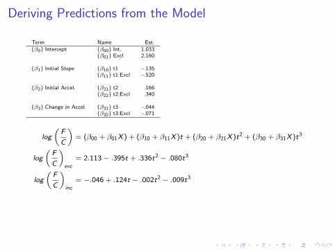
Deriving Predictions from the Model

Term Name Est.(β0) Intercept (β00) Int. 1.033

(β01) Excl 2.160

(β1) Initial Slope (β10) t1 -.135(β11) t1:Excl -.520

(β2) Initial Accel. (β21) t2 .166(β22) t2:Excl .340

(β3) Change in Accel. (β31) t3 -.044(β32) t3:Excl -.071

log

„F

C

«= (β00 + β01X ) + (β10 + β11X )t + (β20 + β21X )t2 + (β30 + β31X )t3

log

„F

C

«exc

= 2.113− .395t + .336t2 − .080t3

log

„F

C

«inc

= −.046 + .124t − .002t2 − .009t3

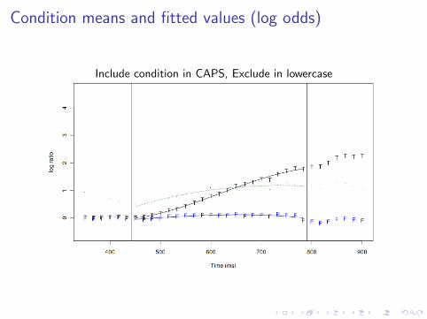
Condition means and fitted values (log odds)

Include condition in CAPS, Exclude in lowercase

Condition means and fitted values (log odds)

Include condition in CAPS, Exclude in lowercase

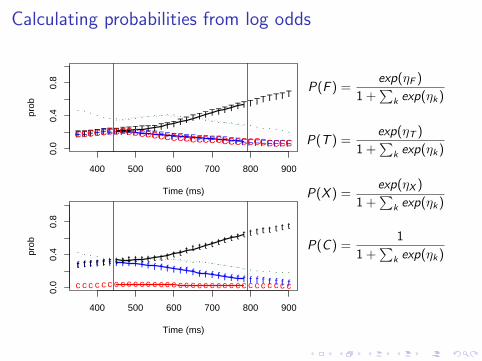
Calculating probabilities from log odds

Let:

ηF = log

(F

C

)= (βF00 + βF01X ) + (βF10 + βF11X )t+

(βF20 + βF21X )t2 + (βF30 + βF31X )t3

ηT = log

(T

C

)= (βT00 + βT01X ) + . . .

ηX = log

(X

C

)= (βX00 + βX01X ) + . . .

Calculating probabilities from log odds

FFFFFFFFFFFFFFFFFFFFFFFFFFFFFFFFFF

400 500 600 700 800 900

0.0

0.4

0.8

Time (ms)

prob

TTTTTTTTTTTTTTTTTTTTTTTTTTTTTTTTTT

CCCCCCCCCCCCCCCCCCCCCCCCCCCCCCCCCC

f f f f f f f f f f f f f f f f f f f f f f f f f f f f f f f f f f

400 500 600 700 800 900

0.0

0.4

0.8

Time (ms)

prob

t t t t t t t t t t t t t t t t t t t t t t t t t t t t t t t t t t

c c c c c c c c c c c c c c c c c c c c c c c c c c c c c c c c c c

P(F ) =exp(ηF )

1 +∑

k exp(ηk)

P(T ) =exp(ηT )

1 +∑

k exp(ηk)

P(X ) =exp(ηX )

1 +∑

k exp(ηk)

P(C ) =1

1 +∑

k exp(ηk)

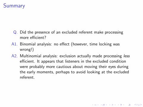
Summary

Q. Did the presence of an excluded referent make processingmore efficient?

A1. Binomial analysis: no effect (however, time locking waswrong!)

A2. Multinomial analysis: exclusion actually made processing lessefficient. It appears that listeners in the excluded conditionwere probably more cautious about moving their eyes duringthe early moments, perhaps to avoid looking at the excludedreferent.

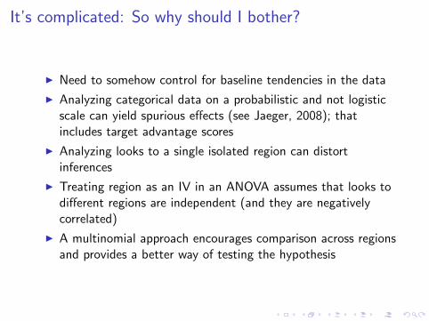
It’s complicated: So why should I bother?

I Need to somehow control for baseline tendencies in the data

I Analyzing categorical data on a probabilistic and not logisticscale can yield spurious effects (see Jaeger, 2008); thatincludes target advantage scores

I Analyzing looks to a single isolated region can distortinferences

I Treating region as an IV in an ANOVA assumes that looks todifferent regions are independent (and they are negativelycorrelated)

I A multinomial approach encourages comparison across regionsand provides a better way of testing the hypothesis

How can I fit a multinomial model?

Dale: Regression-based permutation tests for multilevel data (Rlibrary rbperm and function gmp; I will send you a beta version ifyou email me.)

Austin: Bayesian models with autocorrelated errors using MarkovChain Monte Carlo simulation and Gibbs sampling (please come tohis poster: Frank, Salverda, Jaeger, and Tanenhaus (P196), Postersession 3, Saturday, 12:30-2:30).