Tilburg University

Immigration, Endogenous Technology Adoption and Wages

Ray Chaudhuri, A.; Pandey, Manish

Publication date:2015

Document VersionEarly version, also known as pre-print

Link to publication in Tilburg University Research Portal

Citation for published version (APA):Ray Chaudhuri, A., & Pandey, M. (2015). Immigration, Endogenous Technology Adoption and Wages. (CentERDiscussion Paper; Vol. 2015-008). Department of Economics.

General rightsCopyright and moral rights for the publications made accessible in the public portal are retained by the authors and/or other copyright ownersand it is a condition of accessing publications that users recognise and abide by the legal requirements associated with these rights.

• Users may download and print one copy of any publication from the public portal for the purpose of private study or research. • You may not further distribute the material or use it for any profit-making activity or commercial gain • You may freely distribute the URL identifying the publication in the public portal

Take down policyIf you believe that this document breaches copyright please contact us providing details, and we will remove access to the work immediatelyand investigate your claim.

Download date: 13. Mar. 2022

No. 2015-008

IMMIGRATION, ENDOGENOUS TECHNOLOGY ADOPTION AND WAGES

By

Manish Pandey, Amrita Ray Chaudhuri

27 January, 2015

ISSN 0924-7815 ISSN 2213-9532

Immigration, Endogenous Technology Adoption and Wages∗

Manish Pandey† Amrita Ray Chaudhuri‡

January 27, 2015

Abstract

We document that immigration to U.S. states has increased the mass of workers at the lowerrange of the skill distribution. We use this change in skill distribution of workers to analyzethe effect of immigration on wages. Our model allows firms to endogenously respond tothe immigration-induced changes in skill distribution in terms of their decisions (i) to enterdifferent industries which require the use of different technologies; (ii) to choose acrosstechnologies that differ in their skill-intensity; and (iii) to employ workers of different skilllevels. Allowing these mechanisms to interact, we find that, in line with much of the relatedempirical literature, immigration has a small effect on average real wages of low skilledworkers for U.S. states. We further show that immigration increases the wage inequalitybetween workers of different skill levels in all states, and that the effect of immigrationon wages and wage inequality varies systematically with the volume of immigration acrossstates.

JEL Classification Codes: J61, J31, J24

Keywords: immigration, technology adoption, wages

∗This paper greatly benefited from comments by Wenbiao Cai, Gonzague Vannoorenberghe and seminar partic-ipants at the 2014 Canadian Economics Association Annual Meetings in Vancouver. This research was supportedby funding from the Social Sciences and Humanities Research Council (SSHRC).†University of Winnipeg. Email: m.pandey@uwinnipeg.ca‡University of Winnipeg; CentER & TILEC, Tilburg University. Email: a.raychaudhuri@uwinnipeg.ca

1

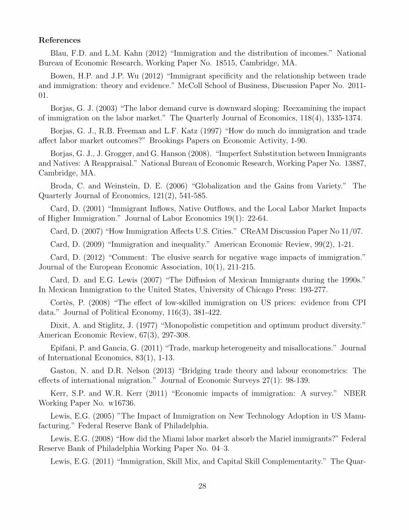
1 Introduction

Immigration volumes have surged in the last decade.1 A natural concern of policy-makers in

countries that receive large inflows of immigrants is whether immigration has adverse effects on

the income of native-born workers.2 A sizeable empirical literature has developed in recent years

to address this issue. According to a recent survey of this literature, a “large majority of studies

suggest that immigration does not exert significant effects on native labor market outcomes”

(Kerr and Kerr, 2011, page 14). Similar conclusions are reached by other surveys, such as

Gaston and Nelson (2013). In particular, studies using city- or state-level data that examine

the impact of immigration on wages in specific labor markets within the U.S. find little to no

negative effects on the wages of native-born workers (see, for example, Card, 2001, 2007; Card

and Lewis, 2007; Lewis, 2011; Ottaviano and Peri, 2012).3 A number of empirical studies have

presented supporting evidence for different possible mechanisms responsible for this recurring

result (Lewis, 2011; Peri, 2012).

Our contribution to this literature is to use a general equilibrium model that integrates

several of the most empirically relevant mechanisms through which immigration affects wages

and examine how the different channels interact and jointly determine the post-immigration

distribution of equilibrium wages across workers with different skill levels. We find that while

immigration of low-skilled workers has a small effect on average real wages of low skilled workers

(in line with the related empirical literature), it increases the wage inequality between workers of

different skill levels by increasing the wages of high-skilled workers. This effect of immigration on

wages and wage inequality varies systematically with the volume of immigration across states.

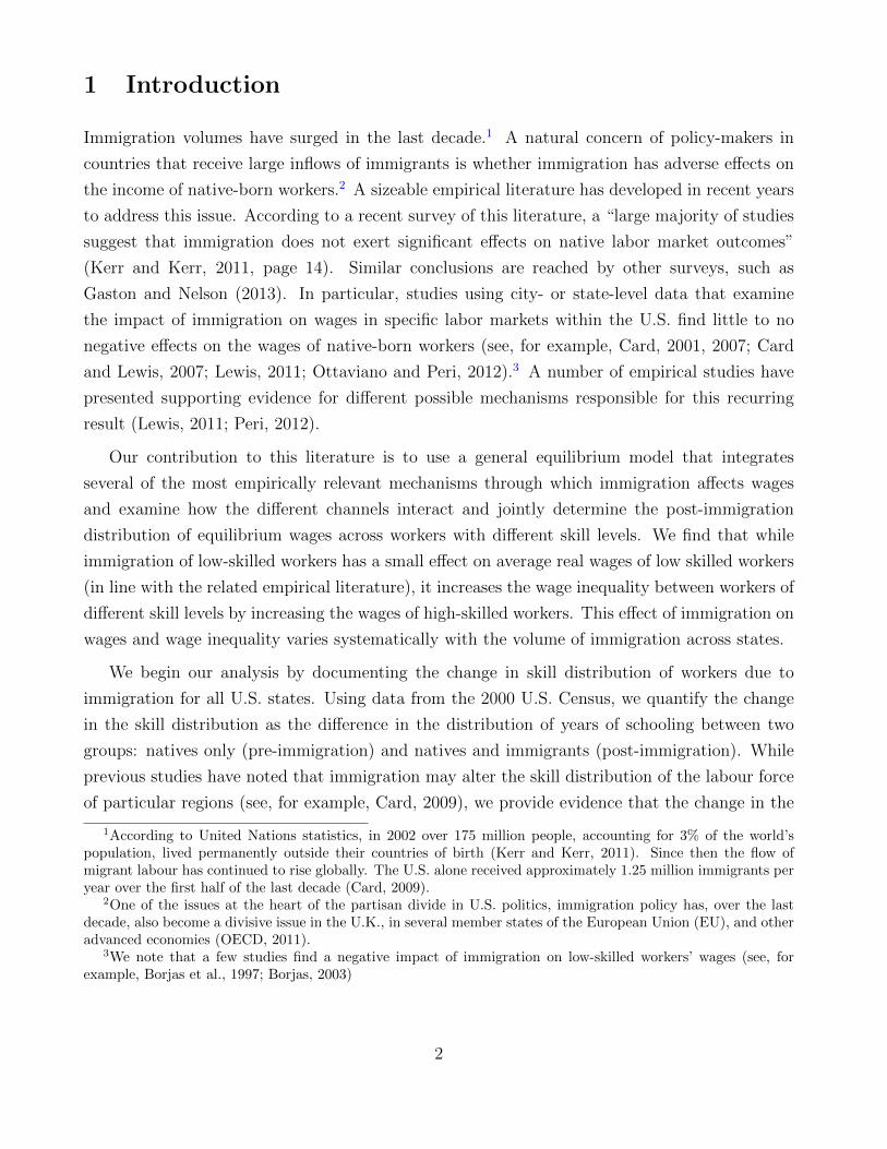
We begin our analysis by documenting the change in skill distribution of workers due to

immigration for all U.S. states. Using data from the 2000 U.S. Census, we quantify the change

in the skill distribution as the difference in the distribution of years of schooling between two

groups: natives only (pre-immigration) and natives and immigrants (post-immigration). While

previous studies have noted that immigration may alter the skill distribution of the labour force

of particular regions (see, for example, Card, 2009), we provide evidence that the change in the

1According to United Nations statistics, in 2002 over 175 million people, accounting for 3% of the world’spopulation, lived permanently outside their countries of birth (Kerr and Kerr, 2011). Since then the flow ofmigrant labour has continued to rise globally. The U.S. alone received approximately 1.25 million immigrants peryear over the first half of the last decade (Card, 2009).

2One of the issues at the heart of the partisan divide in U.S. politics, immigration policy has, over the lastdecade, also become a divisive issue in the U.K., in several member states of the European Union (EU), and otheradvanced economies (OECD, 2011).

3We note that a few studies find a negative impact of immigration on low-skilled workers’ wages (see, forexample, Borjas et al., 1997; Borjas, 2003)

2

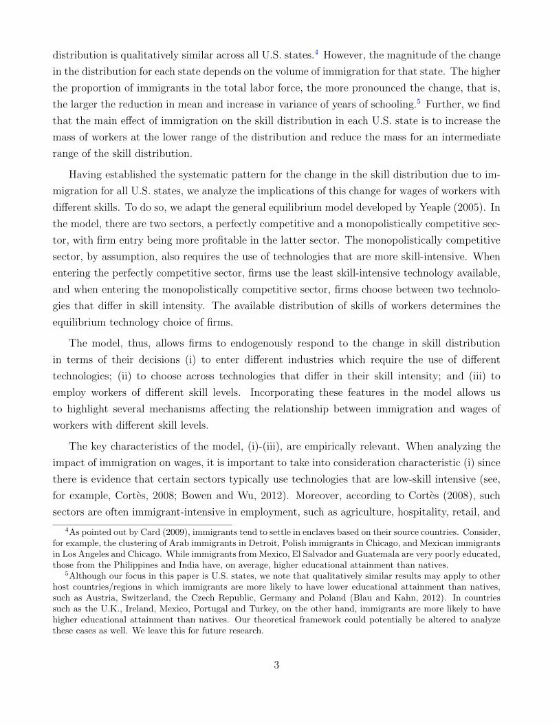
distribution is qualitatively similar across all U.S. states.4 However, the magnitude of the change

in the distribution for each state depends on the volume of immigration for that state. The higher

the proportion of immigrants in the total labor force, the more pronounced the change, that is,

the larger the reduction in mean and increase in variance of years of schooling.5 Further, we find

that the main effect of immigration on the skill distribution in each U.S. state is to increase the

mass of workers at the lower range of the distribution and reduce the mass for an intermediate

range of the skill distribution.

Having established the systematic pattern for the change in the skill distribution due to im-

migration for all U.S. states, we analyze the implications of this change for wages of workers with

different skills. To do so, we adapt the general equilibrium model developed by Yeaple (2005). In

the model, there are two sectors, a perfectly competitive and a monopolistically competitive sec-

tor, with firm entry being more profitable in the latter sector. The monopolistically competitive

sector, by assumption, also requires the use of technologies that are more skill-intensive. When

entering the perfectly competitive sector, firms use the least skill-intensive technology available,

and when entering the monopolistically competitive sector, firms choose between two technolo-

gies that differ in skill intensity. The available distribution of skills of workers determines the

equilibrium technology choice of firms.

The model, thus, allows firms to endogenously respond to the change in skill distribution

in terms of their decisions (i) to enter different industries which require the use of different

technologies; (ii) to choose across technologies that differ in their skill intensity; and (iii) to

employ workers of different skill levels. Incorporating these features in the model allows us

to highlight several mechanisms affecting the relationship between immigration and wages of

workers with different skill levels.

The key characteristics of the model, (i)-(iii), are empirically relevant. When analyzing the

impact of immigration on wages, it is important to take into consideration characteristic (i) since

there is evidence that certain sectors typically use technologies that are low-skill intensive (see,

for example, Cortes, 2008; Bowen and Wu, 2012). Moreover, according to Cortes (2008), such

sectors are often immigrant-intensive in employment, such as agriculture, hospitality, retail, and

4As pointed out by Card (2009), immigrants tend to settle in enclaves based on their source countries. Consider,for example, the clustering of Arab immigrants in Detroit, Polish immigrants in Chicago, and Mexican immigrantsin Los Angeles and Chicago. While immigrants from Mexico, El Salvador and Guatemala are very poorly educated,those from the Philippines and India have, on average, higher educational attainment than natives.

5Although our focus in this paper is U.S. states, we note that qualitatively similar results may apply to otherhost countries/regions in which immigrants are more likely to have lower educational attainment than natives,such as Austria, Switzerland, the Czech Republic, Germany and Poland (Blau and Kahn, 2012). In countriessuch as the U.K., Ireland, Mexico, Portugal and Turkey, on the other hand, immigrants are more likely to havehigher educational attainment than natives. Our theoretical framework could potentially be altered to analyzethese cases as well. We leave this for future research.

3

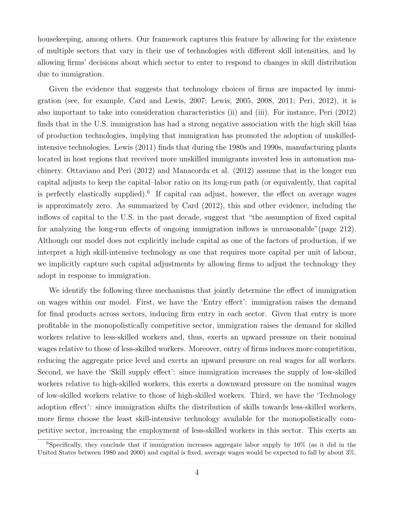
housekeeping, among others. Our framework captures this feature by allowing for the existence

of multiple sectors that vary in their use of technologies with different skill intensities, and by

allowing firms’ decisions about which sector to enter to respond to changes in skill distribution

due to immigration.

Given the evidence that suggests that technology choices of firms are impacted by immi-

gration (see, for example, Card and Lewis, 2007; Lewis, 2005, 2008, 2011; Peri, 2012), it is

also important to take into consideration characteristics (ii) and (iii). For instance, Peri (2012)

finds that in the U.S. immigration has had a strong negative association with the high skill bias

of production technologies, implying that immigration has promoted the adoption of unskilled-

intensive technologies. Lewis (2011) finds that during the 1980s and 1990s, manufacturing plants

located in host regions that received more unskilled immigrants invested less in automation ma-

chinery. Ottaviano and Peri (2012) and Manacorda et al. (2012) assume that in the longer run

capital adjusts to keep the capital–labor ratio on its long-run path (or equivalently, that capital

is perfectly elastically supplied).6 If capital can adjust, however, the effect on average wages

is approximately zero. As summarized by Card (2012), this and other evidence, including the

inflows of capital to the U.S. in the past decade, suggest that “the assumption of fixed capital

for analyzing the long-run effects of ongoing immigration inflows is unreasonable”(page 212).

Although our model does not explicitly include capital as one of the factors of production, if we

interpret a high skill-intensive technology as one that requires more capital per unit of labour,

we implicitly capture such capital adjustments by allowing firms to adjust the technology they

adopt in response to immigration.

We identify the following three mechanisms that jointly determine the effect of immigration

on wages within our model. First, we have the ‘Entry effect’: immigration raises the demand

for final products across sectors, inducing firm entry in each sector. Given that entry is more

profitable in the monopolistically competitive sector, immigration raises the demand for skilled

workers relative to less-skilled workers and, thus, exerts an upward pressure on their nominal

wages relative to those of less-skilled workers. Moreover, entry of firms induces more competition,

reducing the aggregate price level and exerts an upward pressure on real wages for all workers.

Second, we have the ‘Skill supply effect’: since immigration increases the supply of low-skilled

workers relative to high-skilled workers, this exerts a downward pressure on the nominal wages

of low-skilled workers relative to those of high-skilled workers. Third, we have the ‘Technology

adoption effect’: since immigration shifts the distribution of skills towards less-skilled workers,

more firms choose the least skill-intensive technology available for the monopolistically com-

petitive sector, increasing the employment of less-skilled workers in this sector. This exerts an

6Specifically, they conclude that if immigration increases aggregate labor supply by 10% (as it did in theUnited States between 1980 and 2000) and capital is fixed, average wages would be expected to fall by about 3%.

4

upward pressure on the nominal wages of those less-skilled workers who switch employment from

the perfectly competitive to the monopolistically competitive sector.

Having identified the above mechanisms which affect equilibrium wages in different ways

within our theoretical framework, we show analytically that through the interaction of these

mechanisms, immigration increases wage inequality across skill levels both in nominal and real

terms. Moreover, we determine the net effect for U.S. states by quantitatively evaluating the

predictions of the model. We use the change in skill distribution of the labor force for each

state and compute the change in wages as the difference between the pre-immigration and post-

immigration groups. We find that immigration 1) has a small effect on average real wages of low

skilled workers in all states; 2) increases the wage inequality between workers of different skill

levels in all states; and that 3) the magnitudes of the effects of immigration on wages and wage

inequality varies significantly with the volume of immigration across states. The first finding is

consistent with most empirical studies on immigration and wages (see, for example, Card, 2001,

2007; Card and Lewis, 2007; Lewis, 2011; Ottaviano and Peri, 2012). The second finding is in line

with empirical evidence in Card (2009), which suggests that immigration could result in increased

wage inequality. The novel insight generated by our work is that even though immigration has a

small (and often positive) impact on wages of low-skilled workers, it may increase wage inequality

by increasing the wages of high-skilled workers.

The rest of the paper is organized as follows. In Section 2, we document the changes in

the skill distribution of workers due to immigration in U.S. states. In Section 3, we provide a

description of the model and use the model to determine the effects of immigration. Section 4

provides some quantitative results; and Section 5 provides our concluding remarks.

2 Immigration and Changes in Skill Distribution in U.S.

States

In this section we document the changes in the distribution of skill levels of workers due to

immigration for U.S. states; where skill is proxied by educational attainment and age of workers.

Using the 5% sample from the 2000 U.S. Census, we classify an individual as an immigrant

if she/he was not born in the U.S. An individual who is not an immigrant is classified as a

5

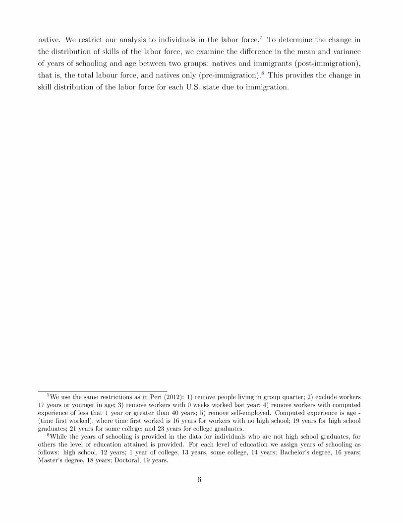
native. We restrict our analysis to individuals in the labor force.7 To determine the change in

the distribution of skills of the labor force, we examine the difference in the mean and variance

of years of schooling and age between two groups: natives and immigrants (post-immigration),

that is, the total labour force, and natives only (pre-immigration).8 This provides the change in

skill distribution of the labor force for each U.S. state due to immigration.

7We use the same restrictions as in Peri (2012): 1) remove people living in group quarter; 2) exclude workers17 years or younger in age; 3) remove workers with 0 weeks worked last year; 4) remove workers with computedexperience of less that 1 year or greater than 40 years; 5) remove self-employed. Computed experience is age -(time first worked), where time first worked is 16 years for workers with no high school; 19 years for high schoolgraduates; 21 years for some college; and 23 years for college graduates.

8While the years of schooling is provided in the data for individuals who are not high school graduates, forothers the level of education attained is provided. For each level of education we assign years of schooling asfollows: high school, 12 years; 1 year of college, 13 years, some college, 14 years; Bachelor’s degree, 16 years;Master’s degree, 18 years; Doctoral, 19 years.

6

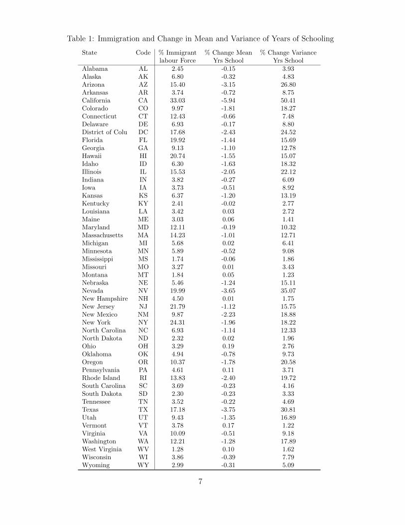
Table 1: Immigration and Change in Mean and Variance of Years of Schooling

State Code % Immigrant % Change Mean % Change Variancelabour Force Yrs School Yrs School

Alabama AL 2.45 -0.15 3.93Alaska AK 6.80 -0.32 4.83Arizona AZ 15.40 -3.15 26.80Arkansas AR 3.74 -0.72 8.75California CA 33.03 -5.94 50.41Colorado CO 9.97 -1.81 18.27Connecticut CT 12.43 -0.66 7.48Delaware DE 6.93 -0.17 8.80District of Colu DC 17.68 -2.43 24.52Florida FL 19.92 -1.44 15.69Georgia GA 9.13 -1.10 12.78Hawaii HI 20.74 -1.55 15.07Idaho ID 6.30 -1.63 18.32Illinois IL 15.53 -2.05 22.12Indiana IN 3.82 -0.27 6.09Iowa IA 3.73 -0.51 8.92Kansas KS 6.37 -1.20 13.19Kentucky KY 2.41 -0.02 2.77Louisiana LA 3.42 0.03 2.72Maine ME 3.03 0.06 1.41Maryland MD 12.11 -0.19 10.32Massachusetts MA 14.23 -1.01 12.71Michigan MI 5.68 0.02 6.41Minnesota MN 5.89 -0.52 9.08Mississippi MS 1.74 -0.06 1.86Missouri MO 3.27 0.01 3.43Montana MT 1.84 0.05 1.23Nebraska NE 5.46 -1.24 15.11Nevada NV 19.99 -3.65 35.07New Hampshire NH 4.50 0.01 1.75New Jersey NJ 21.79 -1.12 15.75New Mexico NM 9.87 -2.23 18.88New York NY 24.31 -1.96 18.22North Carolina NC 6.93 -1.14 12.33North Dakota ND 2.32 0.02 1.96Ohio OH 3.29 0.19 2.76Oklahoma OK 4.94 -0.78 9.73Oregon OR 10.37 -1.78 20.58Pennsylvania PA 4.61 0.11 3.71Rhode Island RI 13.83 -2.40 19.72South Carolina SC 3.69 -0.23 4.16South Dakota SD 2.30 -0.23 3.33Tennessee TN 3.52 -0.22 4.69Texas TX 17.18 -3.75 30.81Utah UT 9.43 -1.35 16.89Vermont VT 3.78 0.17 1.22Virginia VA 10.09 -0.51 9.18Washington WA 12.21 -1.28 17.89West Virginia WV 1.28 0.10 1.62Wisconsin WI 3.86 -0.39 7.79Wyoming WY 2.99 -0.31 5.09

7

For each state, Table 1 reports the share of immigrants in the labor force, and the changes

in the mean and variance of years of schooling due to immigration. As has been documented

by a number of studies, the proportion of immigrants varies significantly across U.S. states (see,

for example, Card, 2009; Lewis, 2011). While California and New York have the highest share

of immigrants in their labour force, at 33% and 24%, respectively, Mississippi (2%) and West

Virginia (1%) have very small proportion of immigrants in their labour force. For most states,

the mean (variance) of years of schooling is lower (higher) for the post-immigration than the

pre-immigration group, indicating that on average immigrants were less educated than natives.

Figure 1: Immigration and Change in Mean Years of Schooling

This is further evident in Figures 1 and 2, which plot changes in mean and variance of years

of schooling due to immigration against the proportion of immigrants in the labor force. As is

clearly evident from the figures, there is a negative (positive) relation between the change in mean

(variance) and proportion of immigrants in the labour force. In other words, if years of schooling

is used as the measure of skills, the change in the skill distribution is systematically related to

the proportion of immigrants in the labor force across U.S. states: the higher the proportion of

immigrants, the larger the reduction in mean and the larger the increase in variance of years of

schooling.

For measuring skill of workers, some studies use data for both education and age of workers

(see, for example, Borjas et al., 2008; Ottavianno and Peri, 2012). Given this, we examine

8

Figure 2: Immigration and Change in Variance of Years of Schooling

whether changes in age of the labor force due to immigration could play an important role in

changing the distribution of skills of the labor force. Figures 3 and 4 plot changes in the mean and

variance of workers’ age due to immigration against the proportion of immigrants in the labour

force. While, similar to mean years of schooling, the change in mean age due to immigration

has a negative relation with the proportion of immigrants, the change in variance of age displays

no relation with the proportion of immigrants. Given that change in mean age and years of

schooling follow a similar pattern across states, the change in age does not add much to the

changes in distribution of skills due to immigration.9

9We use the data on years of schooling and age to estimate a Mincer regression and construct a measure ofskills based on the predicted values from the regression. The Mincer regression we estimate is given by:

lnwi = α+ β ∗ schi + γ1 ∗ expi + γ2 ∗ exp2i + εi,

where for individual i, w is wage income, sch is years of schooling, exp is years of experience measured as(age− 6− school), and ε is an i.i.d. error term. The estimates of the parameters α, β and γ from the regressionare used to predict the logarithm of wages for each individual. This provides a measure of skill that includes botheducation and experience. We estimate the regression separately for the two groups: natives and immigrants andonly natives. The mean and variance of this measure are then compared between the two groups. We find thatthe change in skill distribution due to immigration is very similar to that when skill is measured using only yearsof schooling.

9

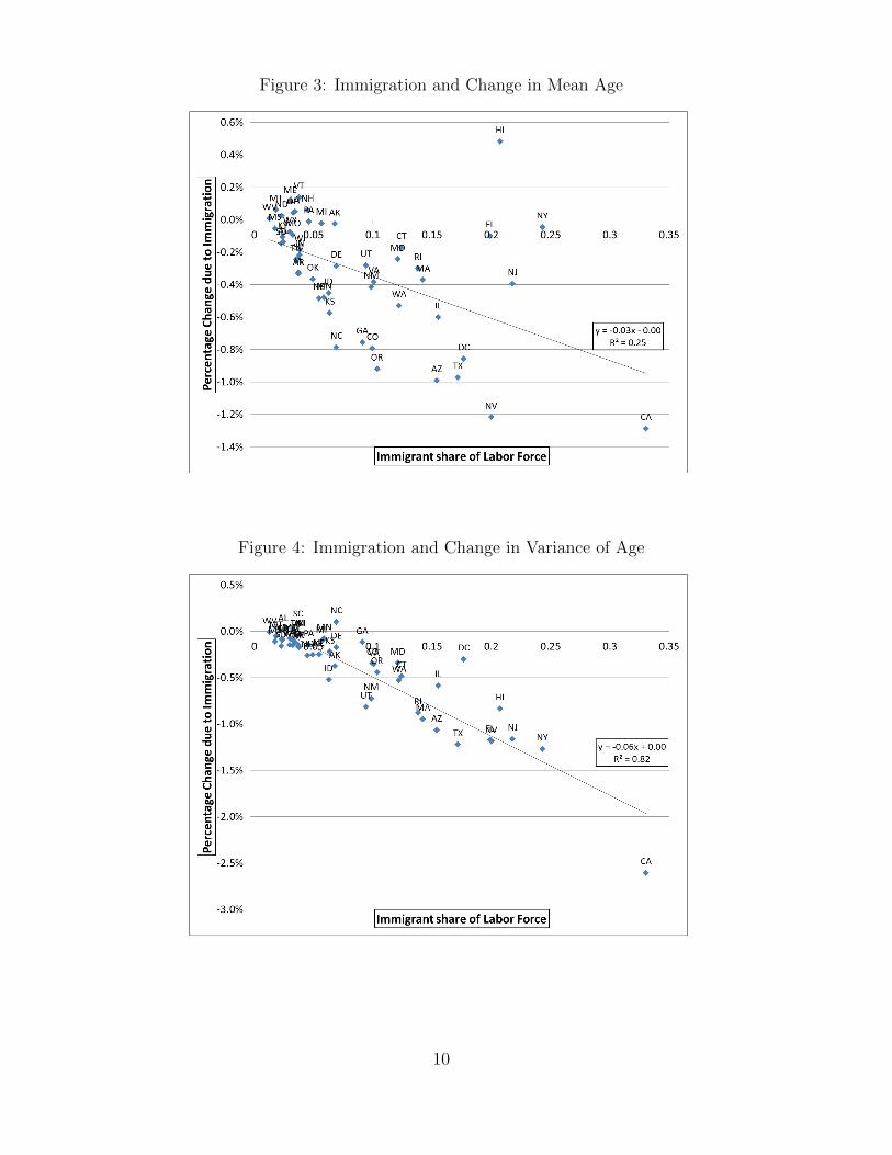
Figure 3: Immigration and Change in Mean Age

Figure 4: Immigration and Change in Variance of Age

10

To illustrate the change in distribution of years of schooling of the labour force due to immi-

gration, Figures 5-8 plot the distribution of years of schooling for the post-immigration and the

pre-immigration groups for the states with the two largest and the two smallest changes in the

the labor force due to immigration. The figures for California and New York clearly indicate that

immigration results in more (less) mass at the lower (intermediate) range of the distribution of

years of schooling of the labor force. A similar shift in the distribution, albeit smaller, is observed

for the U.S. as a whole (Figure 9), and for each individual U.S. state. However, the magnitude

of the shift is smaller for states with smaller change in the labor force due to immigration, such

that for Mississippi and West Virginia there is no visible change in the distribution.

Figure 5: California

0 2 4 6 8 10 12 14 16 180.00

0.05

0.10

0.15

0.20

0.25

0.30

0.35

0.40

0.00

Years of Schooling

Fra

ctio

n of

labo

r fo

rce

post−immigpre−immig

Figure 6: New York

0 2 4 6 8 10 12 14 16 180.00

0.05

0.10

0.15

0.20

0.25

0.30

0.35

0.40

0.00

Years of Schooling

Fra

ctio

n of

labo

r fo

rce

post−immigpre−immig

Figure 7: Mississippi

0 2 4 6 8 10 12 14 16 180.00

0.05

0.10

0.15

0.20

0.25

0.30

0.35

0.40

0.00

Years of Schooling

Fra

ctio

n of

labo

r fo

rce

post−immigpre−immig

Figure 8: West Virginia

0 2 4 6 8 10 12 14 16 180.00

0.05

0.10

0.15

0.20

0.25

0.30

0.35

0.40

0.00

Years of Schooling

Fra

ctio

n of

labo

r fo

rce

post−immigpre−immig

11

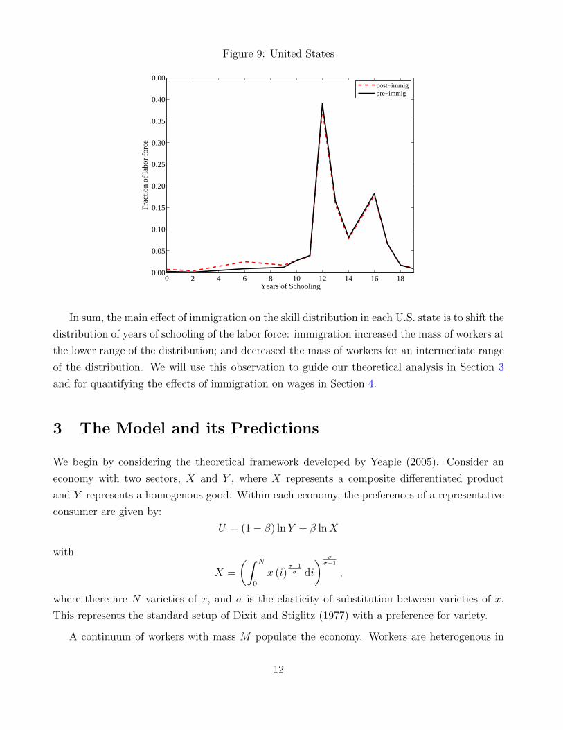
Figure 9: United States

0 2 4 6 8 10 12 14 16 180.00

0.05

0.10

0.15

0.20

0.25

0.30

0.35

0.40

0.00

Years of Schooling

Fra

ctio

n of

labo

r fo

rce

post−immigpre−immig

In sum, the main effect of immigration on the skill distribution in each U.S. state is to shift the

distribution of years of schooling of the labor force: immigration increased the mass of workers at

the lower range of the distribution; and decreased the mass of workers for an intermediate range

of the distribution. We will use this observation to guide our theoretical analysis in Section 3

and for quantifying the effects of immigration on wages in Section 4.

3 The Model and its Predictions

We begin by considering the theoretical framework developed by Yeaple (2005). Consider an

economy with two sectors, X and Y , where X represents a composite differentiated product

and Y represents a homogenous good. Within each economy, the preferences of a representative

consumer are given by:

U = (1− β) lnY + β lnX

with

X =

(∫ N

0

x (i)σ−1σ di

) σσ−1

,

where there are N varieties of x, and σ is the elasticity of substitution between varieties of x.

This represents the standard setup of Dixit and Stiglitz (1977) with a preference for variety.

A continuum of workers with mass M populate the economy. Workers are heterogenous in

12

their skill level, Z; with higher Z, indicating a more skilled worker. There is a continuum of skill

levels, with the distribution of skills across all workers being given by G(Z), density by g(Z) and

support by [0,∞).

There exist two technologies that can be used to produce X, denoted by L and H, and one

technology to produce Y . Let φj(Z) represent the marginal product of a worker with skill level

Z, where j = Y, L,H denotes the technology that the worker is using. It is assumed that the

marginal product of all three technologies increase in Z, that is φ′j(Z) > 0; and that φj(0) = 1

for j = Y, L,H. In addition, it is assumed that marginal product of the three technologies satisfy

the following condition:

∂φH(Z)

∂Z

1

φH(Z)>∂φL(Z)

∂Z

1

φL(Z)>∂φY (Z)

∂Z

1

φY (Z)> 0. (1)

This assumption implies that, relative to all other workers, high skilled workers have a compara-

tive advantage in producing X with technology H; moderate skilled workers are assumed to have

a comparative advantage in producing X with technology L; and workers with the lowest skill

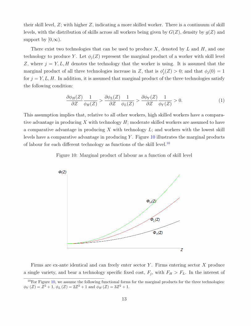
levels have a comparative advantage in producing Y . Figure 10 illustrates the marginal products

of labour for each different technology as functions of the skill level.10

Figure 10: Marginal product of labour as a function of skill level

Firms are ex-ante identical and can freely enter sector Y . Firms entering sector X produce

a single variety, and bear a technology specific fixed cost, Fj, with FH > FL. In the interest of

10For Figure 10, we assume the following functional forms for the marginal products for the three technologies:φY (Z) = Z2 + 1, φL (Z) = 2Z2 + 1 and φH (Z) = 3Z2 + 1.

13

analytical tractability, as in Yeaple (2005), we assume that fixed costs take the form of output that

must be produced in order to enter, but which ultimately cannot be sold. It is assumed that firms

in sector Y are perfectly competitive, setting price equal to marginal cost in equilibrium. The

firms in sector X are monopolistically competitive, setting marginal revenue equal to marginal

cost. Given the functional forms we use, these firms charge a price equal to a constant mark-up

over unit cost. Free entry in both sectors implies that all firms make zero profits in equilibrium.

The pre-immigration equilibrium:

Given the above model setup, the following conditions must be satisfied in equilibrium. Assuming

a perfectly competitive labour market, in equilibrium workers are assigned to technologies such

that the unit costs of all firms using the same technology are equal. The unit cost of producing

with a worker of skill Z, using technology j, is given by W (Z)/φj(Z), where W (Z) is the wage of

a worker with skill level Z. From (1), it follows that, in equilibrium, workers within a range of the

lowest skill levels work in the Y sector, since they have a comparative advantage in producing Y.

Similarly, workers within a range of the highest skill levels work in the X sector using technology

H, since they have a comparative advantage in producing X using technology H. It follows that

workers within an intermediate range of skill levels work in the X sector using technology L,

since they have a comparative advantage in producing X using technology L.11 Let Z1 represent

a threshold such that a worker with skill level Z1 is just indifferent between working in the Y

sector and in the X sector using technology L. Let Z2 represent a threshold such that a worker

with skill level Z2 is just indifferent between working in the X sector using technology L and in

the X sector using technology H. Therefore, in equilibrium, workers with skill Z < Z1 work in

the Y sector, workers with skill Z1 ≤ Z ≤ Z2 work in the X sector and are employed by firms

using technology L, and workers with skill Z > Z2 work in the X sector and are employed by

firms using technology H. It follows that the equilibrium wage distribution is given by:

W (Z) =

CY φY (Z), if 0 ≤ Z ≤ Z1

CLφL(Z), if Z1 ≤ Z ≤ Z2

CHφH(Z), if Z2 ≤ Z <∞

. (2)

where CY , CL, and CH are the unit costs of firms producing with technologies Y, L and H,

respectively. The wage distribution given by (2) implies that firms pay efficiency wages, where

the equilibrium wage of each worker corresponds to the marginal product associated with the

skill level of the worker and the technology he/she uses.

Figure 11 illustrates the equilibrium values of log (W (Z)) as a function of Z. As shown in the

figure, in equilibrium, workers with skill level less than Z1 are employed in sector Y since they

11See Yeaple (2005), Lemma 1 on page 6, for a formal proof.

14

earn a higher wage in sector Y than in other sectors. Similarly, those with skill levels between

Z1 and Z2 are employed in sector X for firms using technology L, and those with skill levels

higher than Z2 are employed in sector X for firms using technology H. The slope of the wage

distribution is increasing at the thresholds, Z1 and Z2 because the value of an additional unit of

workers’ skill is greater for firms using the technologies that are progressively more sensitive to

skill.

Figure 11: Wage distribution

In what follows, it would be useful to determine the relative unit cost of production for each

technology. Let the price of Y, pY , be normalized to 1. Given that the Y sector is perfectly

competitive, we have CY = 1. Recall that, by definition, the threshold Z1 represents that skill

level for which workers are indifferent between working for a firm in sector Y and for a firm in

sector X using technology L. This, together with (2) , implies that

CL =φY (Z1)

φL(Z1)< 1. (3)

Similarly, Z2 represents the skill level for which workers are indifferent between working for a firm

in sector X using technology L, and for a firm in sector X using technology H, which together

15

with (2), implies that

CH =φY (Z1)

φL(Z1)

φL(Z2)

φH(Z2)< CL. (4)

Impact of immigration:

We model immigration as an exogenous shock within the given framework. As shown in Sec-

tion 2, there are two main effects of immigration on the skill distribution in each U.S. state.

First, immigration has systematically increased the mass of workers at the lower tail of the skill

distribution. Second, immigration has systematically decreased the mass of workers for an inter-

mediate range of the skill distribution.12 To reflect these stylized facts, we make the following

assumption. Let Z1 represent the threshold value of Z1 prior to the immigration shock.

Assumption 1: Immigration causes a shift of the density function from g (Z) to g (Z) withg (Z) > g (Z) for 0 <Z < Z1

g (Z) < g (Z) for Z1 <Z < Z2

g (Z) = g (Z) for Z ≥ Z2

The density function g (Z) represents the post-immigration skill distribution with more mass at

the lower tail than the pre-immigration skill distribution, and is associated with the cumulative

distribution function G (Z).13 A direct implication of Assumption 1 are the following Lemmas,

which lead upto Proposition 1.

Lemma 1: Immigration does not affect Z2.

Proof: See Appendix.

Lemma 2: Given Assumption 1, immigration causes a decrease of the threshold Z1 such that

the post-immigration threshold level, Z1, is less than Z1.

Proof: See Appendix.

The change in Z1 due to immigration has implications for the wage distribution across workers

with different skill levels.

Proposition 1: Immigration

(i) does not affect the nominal wages of workers with skill levels 0 ≤ Z ≤ Z1

12Although, in this paper, we focus on the U.S. experience, we note that immigration has changed the skilldistribution in different ways in other countries. For example, in Canada and Australia, educational attainmentsof immigrants are higher on average than that of natives.

13In several U.S. states, the fatter lower tail of the distribution due to immigration occurs for a smaller rangeof Z than 0 < Z < Z1. The theoretical predictions would remain qualitatively similar if Assumption 1 weremodified in line with this.

16

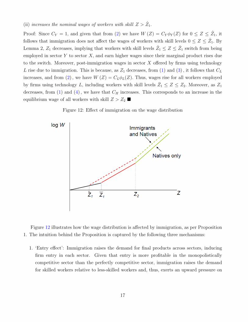
(ii) increases the nominal wages of workers with skill Z > Z1.

Proof: Since CY = 1, and given that from (2) we have W (Z) = CY φY (Z) for 0 ≤ Z ≤ Z1, it

follows that immigration does not affect the wages of workers with skill levels 0 ≤ Z ≤ Z1. By

Lemma 2, Z1 decreases, implying that workers with skill levels Z1 ≤ Z ≤ Z1 switch from being

employed in sector Y to sector X, and earn higher wages since their marginal product rises due

to the switch. Moreover, post-immigration wages in sector X offered by firms using technology

L rise due to immigration. This is because, as Z1 decreases, from (1) and (3) , it follows that CL

increases, and from (2) , we have W (Z) = CLφL(Z). Thus, wages rise for all workers employed

by firms using technology L, including workers with skill levels Z1 ≤ Z ≤ Z2. Moreover, as Z1

decreases, from (1) and (4) , we have that CH increases. This corresponds to an increase in the

equilibrium wage of all workers with skill Z > Z2 �

Figure 12: Effect of immigration on the wage distribution

Figure 12 illustrates how the wage distribution is affected by immigration, as per Proposition

1. The intuition behind the Proposition is captured by the following three mechanisms:

1. ‘Entry effect’: Immigration raises the demand for final products across sectors, inducing

firm entry in each sector. Given that entry is more profitable in the monopolistically

competitive sector than the perfectly competitive sector, immigration raises the demand

for skilled workers relative to less-skilled workers and, thus, exerts an upward pressure on

17

their nominal wages relative to those of less-skilled workers.14

2. ‘Skill supply effect’: Since immigration increases the supply of low-skilled workers relative

to high-skilled workers, this exerts a downward pressure on the nominal wages of low-skilled

workers relative to those of high-skilled workers.

3. ‘Technology adoption effect’: Since immigration shifts the distribution of skills towards

less-skilled workers, more firms choose the least skill-intensive technology available for the

monopolistically competitive sector, increasing the employment of less-skilled workers in

this sector. This exerts an upward pressure on the nominal wages of those of the less-skilled

workers who switch employment from the perfectly competitive to the monopolistically

competitive sector.

The ‘Technology adoption effect’ is seen for workers with skill levels Z1 ≤ Z ≤ Z1, who

switch from sector Y to sector X, and consequently earn higher nominal wages. The ‘Entry

effect’ and the ‘Skill supply effect’ together explain why, in Figure 1, we see an increase in wage

inequality across skill levels with high skilled workers experiencing higher increases in nominal

wages relative to low-skilled workers. More specifically, immigration leads to an increase in

the wages of workers with skill greater than Z1 relative to those with skills below Z1. This is

consistent with the conclusion of Card (2009) [p.19] that “...wage inequality over all workers in

the economy is higher than it would be in the absence of immigration.”

Proposition 2: The effect of immigration on real wages is ambiguous. The larger the immigration-

induced increase in the mass of workers,M, the more likely that real wages increase. Immigration

increases real wage inequality across skill levels.

Proof: The aggregate price level is given by:15

14Let NL and NH represent the equilibrium number of firms to enter the X sector and choose technology Land H respectively. From the zero profits conditions, it can be shown that:

NH =M

σ (FH)

∫ ∞Z2

φH(Z)dG (Z)

NL =M

σFL

∫ Z2

Z1

φL(Z)dG (Z)

For further details of the derivation of NL and NH , please refer to Yeaple (2005), equations (11) and (12). Sinceimmigration increases the mass of workers, M , and does not affect Z2 (by Lemma 1), NH increases due toimmigration. Since immigration increases M, decreases Z1 (by Lemma 2) and does not affect Z2 (by Lemma 1),there is an upward pressure on NL. At the same time, by Assumption 1, since g (Z) < g (Z) for Z1 <Z < Z2,thereis a downward pressure on NL. Thus, the net effect on NL is ambiguous. Since NL is increasing in M, the greaterthe immigration-induced increase in M, the more likely that the net effect on NL is positive.

15The derivation of PX follows directly from the fact that under the standard Dixit-Stiglitz framework, eachfirm charges a constant mark-up of σ

σ−1 over its unit cost.

18

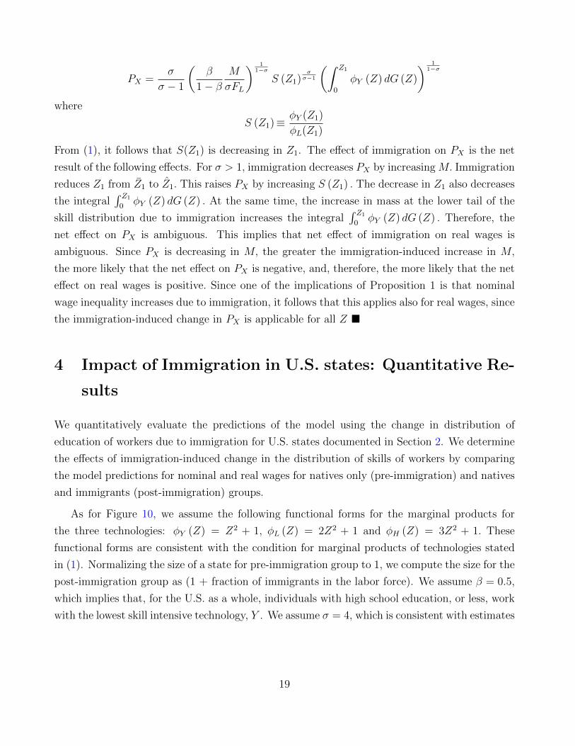
PX =σ

σ − 1

(β

1− βM

σFL

) 11−σ

S (Z1)σσ−1

(∫ Z1

0

φY (Z) dG (Z)

) 11−σ

where

S (Z1)≡ φY (Z1)

φL(Z1)

From (1), it follows that S(Z1) is decreasing in Z1. The effect of immigration on PX is the net

result of the following effects. For σ > 1, immigration decreases PX by increasing M. Immigration

reduces Z1 from Z1 to Z1. This raises PX by increasing S (Z1) . The decrease in Z1 also decreases

the integral∫ Z1

0φY (Z) dG (Z) . At the same time, the increase in mass at the lower tail of the

skill distribution due to immigration increases the integral∫ Z1

0φY (Z) dG (Z) . Therefore, the

net effect on PX is ambiguous. This implies that net effect of immigration on real wages is

ambiguous. Since PX is decreasing in M, the greater the immigration-induced increase in M,

the more likely that the net effect on PX is negative, and, therefore, the more likely that the net

effect on real wages is positive. Since one of the implications of Proposition 1 is that nominal

wage inequality increases due to immigration, it follows that this applies also for real wages, since

the immigration-induced change in PX is applicable for all Z �

4 Impact of Immigration in U.S. states: Quantitative Re-

sults

We quantitatively evaluate the predictions of the model using the change in distribution of

education of workers due to immigration for U.S. states documented in Section 2. We determine

the effects of immigration-induced change in the distribution of skills of workers by comparing

the model predictions for nominal and real wages for natives only (pre-immigration) and natives

and immigrants (post-immigration) groups.

As for Figure 10, we assume the following functional forms for the marginal products for

the three technologies: φY (Z) = Z2 + 1, φL (Z) = 2Z2 + 1 and φH (Z) = 3Z2 + 1. These

functional forms are consistent with the condition for marginal products of technologies stated

in (1). Normalizing the size of a state for pre-immigration group to 1, we compute the size for the

post-immigration group as (1 + fraction of immigrants in the labor force). We assume β = 0.5,

which implies that, for the U.S. as a whole, individuals with high school education, or less, work

with the lowest skill intensive technology, Y . We assume σ = 4, which is consistent with estimates

19

of the elasticity of substitution for preference for variety utility functions.16 Further, we assume

that to be employed by firms using the H technology, workers need to have completed 4-year

college education or more (16 or more years of schooling). Since the value of Z2 is independent

of changes in skill distribution or increase in size of the labour force (Lemma 1), the value for

this threshold is same for both the pre- and post-immigration groups.

For each state, we use the educational attainment distribution of the labor force (skill dis-

tribution) discussed in Section 2 for the pre- and post-immigration groups and solve for the

equilibrium values. In particular, given the skill distribution, we solve for threshold Z1 and then

compute the employment and wages in each sector for the two groups. The effect of immigration

is computed as the difference in outcomes for the two groups. Given that California and New

York were the states with the highest fraction of immigrants in the labor force, 33% and 24%

respectively, (see Table 1), we begin the discussion with the results for these two states.

Given that due to immigration more workers with lower levels of education enter the labor

force for both states (Figures 5 and 6), in line with Lemma 2, there is a decrease in the skill

threshold below which workers are employed with the Y technology, Z1. Figure 13 provides

the effect of immigration on the wage distribution for California. The pattern of the change

is consistent with the theoretical prediction summarized in Proposition 1 and Figure 12. In

Figure 13, we clearly observe the Technology adoption effect at work, causing workers with skill

Z1 ≤ Z ≤ Z1 to switch from Y to X, and earn higher nominal wages. We note that a qualitatively

similar pattern emerges for all U.S. states.

Table 2: Change in Wages (%)

Wnom Wreal

CaliforniaY -3.67 2.94L -0.58 6.25H 1.04 7.97

New YorkY -1.29 3.28L -0.48 4.13H 0.65 5.30

Table 2 summarizes the results of the effect of immigration on wages for California and New

York. Immigration results in a decrease in average nominal wages of workers employed with Y

and L, but a small increase in average wages for workers employed with H. The average wages

for workers employed with Y and L decrease because of a decrease in the average skill level

16The value of σ we use in the range of the estimates of the elasticity of substitution in the literature (see Brodaand Weinstein, 2006; and Epifani and Gancia, 2011).

20

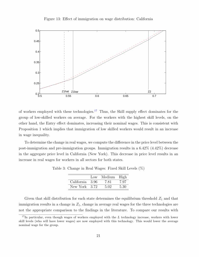
Figure 13: Effect of immigration on wage distribution: California

0.5 0.55 0.6 0.65 0.70.2

0.25

0.3

0.35

0.4

0.45

0.5

Z1hat Z1bar Z2

of workers employed with these technologies.17 Thus, the Skill supply effect dominates for the

group of low-skilled workers on average. For the workers with the highest skill levels, on the

other hand, the Entry effect dominates, increasing their nominal wages. This is consistent with

Proposition 1 which implies that immigration of low skilled workers would result in an increase

in wage inequality.

To determine the change in real wages, we compute the difference in the price level between the

post-immigration and pre-immigration groups. Immigration results in a 6.42% (4.42%) decrease

in the aggregate price level in California (New York). This decrease in price level results in an

increase in real wages for workers in all sectors for both states.

Table 3: Change in Real Wages: Fixed Skill Levels (%)

Low Medium HighCalifornia 3.96 7.81 7.97New York 3.72 5.02 5.30

Given that skill distribution for each state determines the equilibrium threshold Z1 and that

immigration results in a change in Z1, change in average real wages for the three technologies are

not the appropriate comparison to the findings in the literature. To compare our results with

17In particular, even though wages of workers employed with the L technology increase, workers with lowerskill levels (who will have lower wages) are now employed with this technology. This would lower the averagenominal wage for the group.

21

the empirical findings in the literature we need to fix skill levels. Consistent with the definitions

in the literature (Borjas, 2003; Borjas et al., 2008; Card, 2009; Ottaviano and Peri, 2012, among

others), we define low skilled, Low, as workers with education level of high school or less, middle

skilled, Medium, as workers with some college and high skilled, High, as workers who have

complete university degrees. Using this definition we compute the change in the real wage for

low, medium and high skilled workers between the post-immigration and pre-immigration groups.

Table 3 provide the results for California and New York. Immigration results in an increase in

average real wages for all the three skill levels. In other words, whether we examine changes for

the three technologies or for fixed skill levels, immigration results in an increase in average real

wages for workers with the gains being higher for high skilled than low skilled workers. Therefore,

our findings are in line with evidence in Card (2009)which suggests that immigration to the U.S.

could result in an increase in wage inequality.

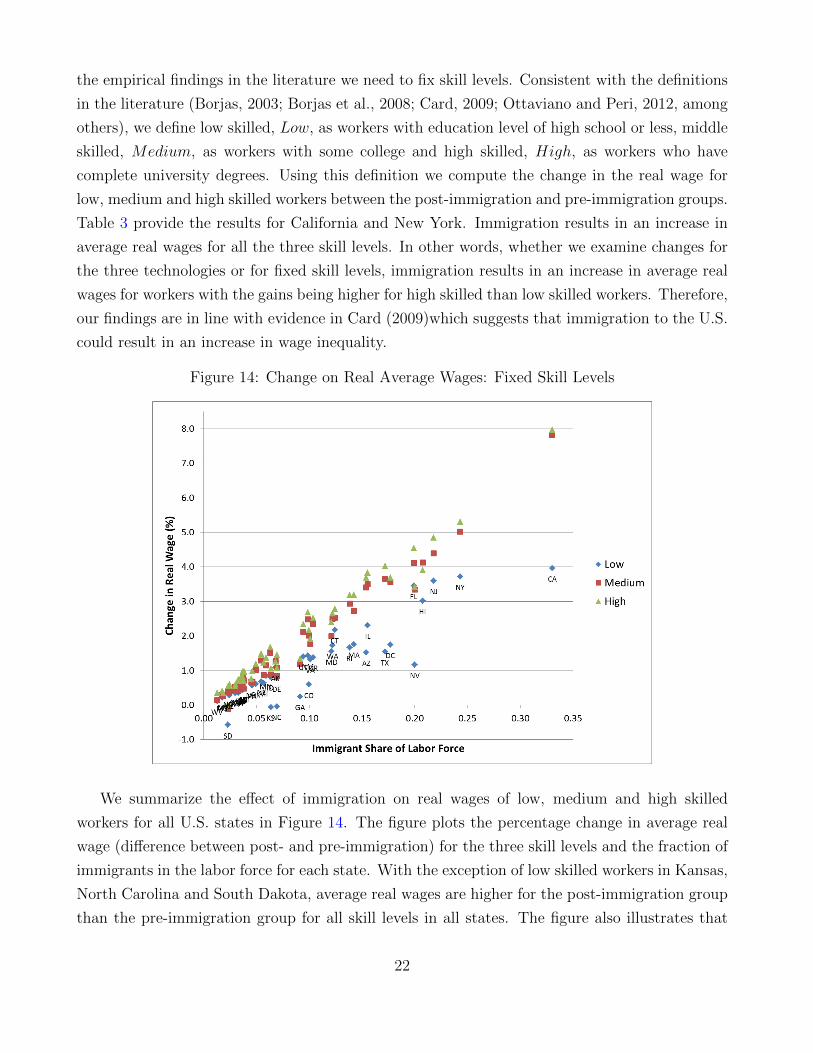
Figure 14: Change on Real Average Wages: Fixed Skill Levels

We summarize the effect of immigration on real wages of low, medium and high skilled

workers for all U.S. states in Figure 14. The figure plots the percentage change in average real

wage (difference between post- and pre-immigration) for the three skill levels and the fraction of

immigrants in the labor force for each state. With the exception of low skilled workers in Kansas,

North Carolina and South Dakota, average real wages are higher for the post-immigration group

than the pre-immigration group for all skill levels in all states. The figure also illustrates that

22

the difference in average real wages between the two groups are 1) lower for low skilled workers

than medium and high skilled workers; and 2) positively related to the fraction of immigrants in

the labor force. In sum, similar to the findings for California and New York, immigration results

in an increase in wage inequality in all states, with the increase being higher for states with a

higher fraction of immigrants in the labor force.

4.1 Robustness

We examine the robustness of our quantitative findings by relaxing some of the assumptions

made for computing the effects of immigration on wages.

4.1.1 Trade and Labor mobility

We assumed that the U.S. states are in autarky (prices differ across states) and that there is

no mobility of labor between states (wages differ across states). We relax these assumptions by

computing the effect of immigration using the change in skill distribution due to immigration for

the U.S. as a whole (Figure 9), which would imply integrated goods and labor markets for the

whole of U.S. In other words, through mobility of goods and/or labor across states, the effects

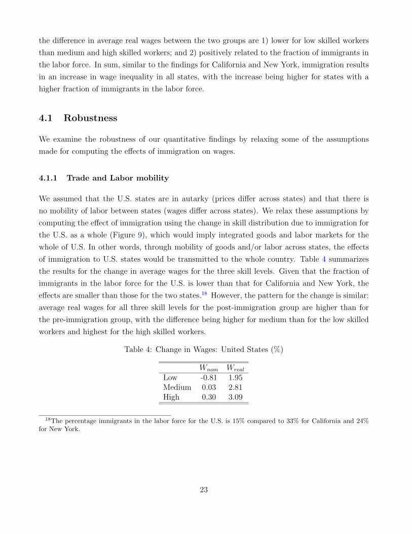
of immigration to U.S. states would be transmitted to the whole country. Table 4 summarizes

the results for the change in average wages for the three skill levels. Given that the fraction of

immigrants in the labor force for the U.S. is lower than that for California and New York, the

effects are smaller than those for the two states.18 However, the pattern for the change is similar:

average real wages for all three skill levels for the post-immigration group are higher than for

the pre-immigration group, with the difference being higher for medium than for the low skilled

workers and highest for the high skilled workers.

Table 4: Change in Wages: United States (%)

Wnom Wreal

Low -0.81 1.95Medium 0.03 2.81High 0.30 3.09

18The percentage immigrants in the labor force for the U.S. is 15% compared to 33% for California and 24%for New York.

23

4.1.2 Sensitivity of Results: Parameter Values

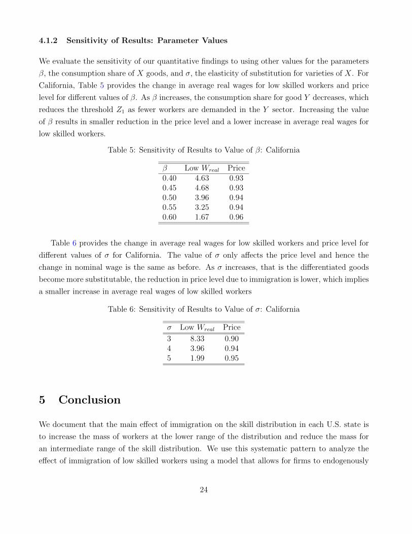
We evaluate the sensitivity of our quantitative findings to using other values for the parameters

β, the consumption share of X goods, and σ, the elasticity of substitution for varieties of X. For

California, Table 5 provides the change in average real wages for low skilled workers and price

level for different values of β. As β increases, the consumption share for good Y decreases, which

reduces the threshold Z1 as fewer workers are demanded in the Y sector. Increasing the value

of β results in smaller reduction in the price level and a lower increase in average real wages for

low skilled workers.

Table 5: Sensitivity of Results to Value of β: California

β Low Wreal Price0.40 4.63 0.930.45 4.68 0.930.50 3.96 0.940.55 3.25 0.940.60 1.67 0.96

Table 6 provides the change in average real wages for low skilled workers and price level for

different values of σ for California. The value of σ only affects the price level and hence the

change in nominal wage is the same as before. As σ increases, that is the differentiated goods

become more substitutable, the reduction in price level due to immigration is lower, which implies

a smaller increase in average real wages of low skilled workers

Table 6: Sensitivity of Results to Value of σ: California

σ Low Wreal Price

3 8.33 0.904 3.96 0.945 1.99 0.95

5 Conclusion

We document that the main effect of immigration on the skill distribution in each U.S. state is

to increase the mass of workers at the lower range of the distribution and reduce the mass for

an intermediate range of the skill distribution. We use this systematic pattern to analyze the

effect of immigration of low skilled workers using a model that allows for firms to endogenously

24

respond to changes in the skill distribution due to immigration. In particular, firms respond by

entering different industries and/or choosing different technologies.

We identify three mechanisms in the model that jointly determine the effect of immigration on

wages of workers with different skills. First, the ‘Entry effect’ through which immigration raises

the demand for goods for all sectors, inducing entry of firms. Since entry is more profitable

into the sector requiring a high skill intensive technology, this exerts an upward pressure on

high-skilled workers’ wages. Second, the ‘Skill supply effect’ through which immigration of low

skilled workers exerts downward pressure on the wages of these workers. Third, the ‘Technology

adoption effect’ through which the change in the skill distribution towards low skilled workers

leads to more firms choosing less skill intensive technologies and thus increasing the demand for

low skilled workers. We show analytically that the interaction of these mechanisms increase wage

inequality across skill levels both in nominal and real terms.

Moreover, we illustrate the net effect for U.S. states by quantitatively evaluating the predic-

tions of the model. For each state we compute the difference in wages for the pre-immigration and

post-immigration skill distributions. We find that immigration 1) has a small effect on average

real wages of low skilled workers in all states; 2) increases the wage inequality between workers

of different skill levels in all states; and that 3) the magnitudes of the effects of immigration

on wages and wage inequality varies significantly with the volume of immigration across states.

The novel insight generated by our work is that immigration increases wage inequality not by

decreasing the wages of low-skilled workers, rather by increasing the wages of high-skilled workers

while having a small impact on wages of low-skilled workers. While our results are consistent

with the existing empirical literature which concludes that immigration has a small impact on

wages of low-skilled workers, a useful avenue for future empirical research would be to further

explore our predictions regarding the effect of immigration on wage inequality.

25

Appendix:

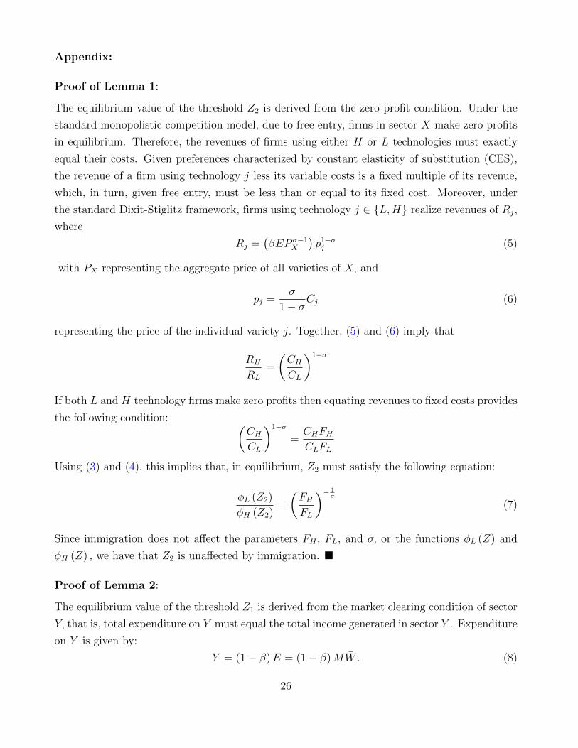
Proof of Lemma 1:

The equilibrium value of the threshold Z2 is derived from the zero profit condition. Under the

standard monopolistic competition model, due to free entry, firms in sector X make zero profits

in equilibrium. Therefore, the revenues of firms using either H or L technologies must exactly

equal their costs. Given preferences characterized by constant elasticity of substitution (CES),

the revenue of a firm using technology j less its variable costs is a fixed multiple of its revenue,

which, in turn, given free entry, must be less than or equal to its fixed cost. Moreover, under

the standard Dixit-Stiglitz framework, firms using technology j ∈ {L,H} realize revenues of Rj,

where

Rj =(βEP σ−1

X

)p1−σj (5)

with PX representing the aggregate price of all varieties of X, and

pj =σ

1− σCj (6)

representing the price of the individual variety j. Together, (5) and (6) imply that

RH

RL

=

(CHCL

)1−σ

If both L and H technology firms make zero profits then equating revenues to fixed costs provides

the following condition: (CHCL

)1−σ

=CHFHCLFL

Using (3) and (4), this implies that, in equilibrium, Z2 must satisfy the following equation:

φL (Z2)

φH (Z2)=

(FHFL

)− 1σ

(7)

Since immigration does not affect the parameters FH , FL, and σ, or the functions φL (Z) and

φH (Z) , we have that Z2 is unaffected by immigration. �

Proof of Lemma 2:

The equilibrium value of the threshold Z1 is derived from the market clearing condition of sector

Y, that is, total expenditure on Y must equal the total income generated in sector Y . Expenditure

on Y is given by:

Y = (1− β)E = (1− β)MW. (8)

26

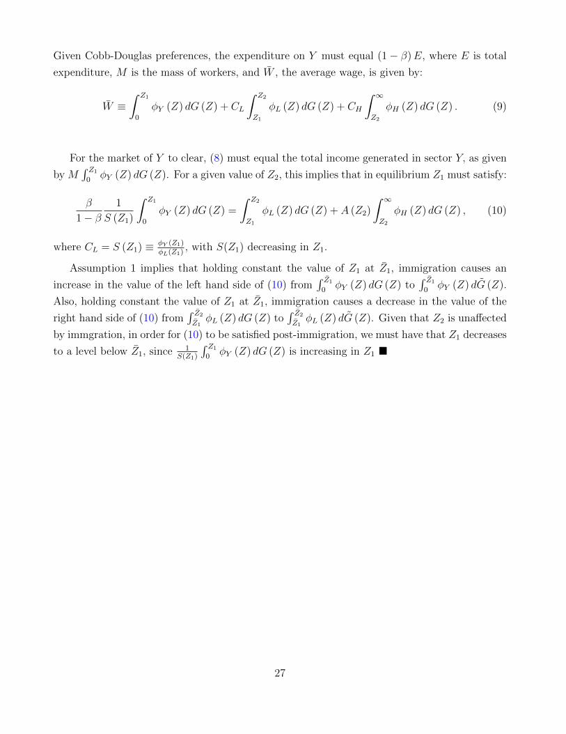
Given Cobb-Douglas preferences, the expenditure on Y must equal (1− β)E, where E is total

expenditure, M is the mass of workers, and W , the average wage, is given by:

W ≡∫ Z1

0

φY (Z) dG (Z) + CL

∫ Z2

Z1

φL (Z) dG (Z) + CH

∫ ∞Z2

φH (Z) dG (Z) . (9)

For the market of Y to clear, (8) must equal the total income generated in sector Y, as given

by M∫ Z1

0φY (Z) dG (Z). For a given value of Z2, this implies that in equilibrium Z1 must satisfy:

β

1− β1

S (Z1)

∫ Z1

0

φY (Z) dG (Z) =

∫ Z2

Z1

φL (Z) dG (Z) + A (Z2)

∫ ∞Z2

φH (Z) dG (Z) , (10)

where CL = S (Z1) ≡ φY (Z1)φL(Z1)

, with S(Z1) decreasing in Z1.

Assumption 1 implies that holding constant the value of Z1 at Z1, immigration causes an

increase in the value of the left hand side of (10) from∫ Z1

0φY (Z) dG (Z) to

∫ Z1

0φY (Z) dG (Z).

Also, holding constant the value of Z1 at Z1, immigration causes a decrease in the value of the

right hand side of (10) from∫ Z2

Z1φL (Z) dG (Z) to

∫ Z2

Z1φL (Z) dG (Z). Given that Z2 is unaffected

by immgration, in order for (10) to be satisfied post-immigration, we must have that Z1 decreases

to a level below Z1, since 1S(Z1)

∫ Z1

0φY (Z) dG (Z) is increasing in Z1 �

27

References

Blau, F.D. and L.M. Kahn (2012) “Immigration and the distribution of incomes.” NationalBureau of Economic Research, Working Paper No. 18515, Cambridge, MA.

Bowen, H.P. and J.P. Wu (2012) “Immigrant specificity and the relationship between tradeand immigration: theory and evidence.” McColl School of Business, Discussion Paper No. 2011-01.

Borjas, G. J. (2003) “The labor demand curve is downward sloping: Reexamining the impactof immigration on the labor market.” The Quarterly Journal of Economics, 118(4), 1335-1374.

Borjas, G. J., R.B. Freeman and L.F. Katz (1997) “How do much do immigration and tradeaffect labor market outcomes?” Brookings Papers on Economic Activity, 1-90.

Borjas, G. J., J. Grogger, and G. Hanson (2008). “Imperfect Substitution between Immigrantsand Natives: A Reappraisal.” National Bureau of Economic Research, Working Paper No. 13887,Cambridge, MA.

Broda, C. and Weinstein, D. E. (2006) “Globalization and the Gains from Variety.” TheQuarterly Journal of Economics, 121(2), 541-585.

Card, D. (2001) “Immigrant Inflows, Native Outflows, and the Local Labor Market Impactsof Higher Immigration.” Journal of Labor Economics 19(1): 22-64.

Card, D. (2007) “How Immigration Affects U.S. Cities.” CReAM Discussion Paper No 11/07.

Card, D. (2009) “Immigration and inequality.” American Economic Review, 99(2), 1-21.

Card, D. (2012) “Comment: The elusive search for negative wage impacts of immigration.”Journal of the European Economic Association, 10(1), 211-215.

Card, D. and E.G. Lewis (2007) “The Diffusion of Mexican Immigrants during the 1990s.”In Mexican Immigration to the United States, University of Chicago Press: 193-277.

Cortes, P. (2008) “The effect of low-skilled immigration on US prices: evidence from CPIdata.” Journal of Political Economy, 116(3), 381-422.

Dixit, A. and Stiglitz, J. (1977) “Monopolistic competition and optimum product diversity.”American Economic Review, 67(3), 297-308.

Epifani, P. and Gancia, G. (2011) “Trade, markup heterogeneity and misallocations.” Journalof International Economics, 83(1), 1-13.

Gaston, N. and D.R. Nelson (2013) “Bridging trade theory and labour econometrics: Theeffects of international migration.” Journal of Economic Surveys 27(1): 98-139.

Kerr, S.P. and W.R. Kerr (2011) “Economic impacts of immigration: A survey.” NBERWorking Paper No. w16736.

Lewis, E.G. (2005) ”The Impact of Immigration on New Technology Adoption in US Manu-facturing.” Federal Reserve Bank of Philadelphia.

Lewis, E.G. (2008) “How did the Miami labor market absorb the Mariel immigrants?” FederalReserve Bank of Philadelphia Working Paper No. 04–3.

Lewis, E.G. (2011) “Immigration, Skill Mix, and Capital Skill Complementarity.” The Quar-

28

terly Journal of Economics, 126(2), 1029-1069.

Manacorda, M., A. Manning and J. Wadsworth (2012) “The impact of immigration on thestructure of male wages: Theory and evidence for Britain.” Journal of the European EconomicAssociation 10(1), 120-151.

Organization for Economic Cooperation and Development (OECD)(2011) “International Mi-gration and the SOPEMI.”

Ottaviano, G. I. P. and G. Peri (2012) “Rethinking the effects of immigration on wages.”Journal of the European Economic Association 10(1), 152-197

Peri, G. (2012) “The Effect Of Immigration On Productivity: Evidence From US States.”The Review of Economics and Statistics, 94(1), 348-358.

Yeaple, S. (2005) “A simple model of firm heterogeneity, international trade, and wages.”Journal of International Economics, 65(1), 1-20.

29

Immigration, Endogenous Technology Adoption and Wages∗

Manish Pandey† Amrita Ray Chaudhuri‡

January 27, 2015

Abstract

We document that immigration to U.S. states has increased the mass of workers at the lowerrange of the skill distribution. We use this change in skill distribution of workers to analyzethe effect of immigration on wages. Our model allows firms to endogenously respond tothe immigration-induced changes in skill distribution in terms of their decisions (i) to enterdifferent industries which require the use of different technologies; (ii) to choose acrosstechnologies that differ in their skill-intensity; and (iii) to employ workers of different skilllevels. Allowing these mechanisms to interact, we find that, in line with much of the relatedempirical literature, immigration has a small effect on average real wages of low skilledworkers for U.S. states. We further show that immigration increases the wage inequalitybetween workers of different skill levels in all states, and that the effect of immigrationon wages and wage inequality varies systematically with the volume of immigration acrossstates.

JEL Classification Codes: J61, J31, J24

Keywords: immigration, technology adoption, wages

∗This paper greatly benefited from comments by Wenbiao Cai, Gonzague Vannoorenberghe and seminar partic-ipants at the 2014 Canadian Economics Association Annual Meetings in Vancouver. This research was supportedby funding from the Social Sciences and Humanities Research Council (SSHRC).†University of Winnipeg. Email: m.pandey@uwinnipeg.ca‡University of Winnipeg; CentER & TILEC, Tilburg University. Email: a.raychaudhuri@uwinnipeg.ca

1

1 Introduction

Immigration volumes have surged in the last decade.1 A natural concern of policy-makers in

countries that receive large inflows of immigrants is whether immigration has adverse effects on

the income of native-born workers.2 A sizeable empirical literature has developed in recent years

to address this issue. According to a recent survey of this literature, a “large majority of studies

suggest that immigration does not exert significant effects on native labor market outcomes”

(Kerr and Kerr, 2011, page 14). Similar conclusions are reached by other surveys, such as

Gaston and Nelson (2013). In particular, studies using city- or state-level data that examine

the impact of immigration on wages in specific labor markets within the U.S. find little to no

negative effects on the wages of native-born workers (see, for example, Card, 2001, 2007; Card

and Lewis, 2007; Lewis, 2011; Ottaviano and Peri, 2012).3 A number of empirical studies have

presented supporting evidence for different possible mechanisms responsible for this recurring

result (Lewis, 2011; Peri, 2012).

Our contribution to this literature is to use a general equilibrium model that integrates

several of the most empirically relevant mechanisms through which immigration affects wages

and examine how the different channels interact and jointly determine the post-immigration

distribution of equilibrium wages across workers with different skill levels. We find that while

immigration of low-skilled workers has a small effect on average real wages of low skilled workers

(in line with the related empirical literature), it increases the wage inequality between workers of

different skill levels by increasing the wages of high-skilled workers. This effect of immigration on

wages and wage inequality varies systematically with the volume of immigration across states.

We begin our analysis by documenting the change in skill distribution of workers due to

immigration for all U.S. states. Using data from the 2000 U.S. Census, we quantify the change

in the skill distribution as the difference in the distribution of years of schooling between two

groups: natives only (pre-immigration) and natives and immigrants (post-immigration). While

previous studies have noted that immigration may alter the skill distribution of the labour force

of particular regions (see, for example, Card, 2009), we provide evidence that the change in the

1According to United Nations statistics, in 2002 over 175 million people, accounting for 3% of the world’spopulation, lived permanently outside their countries of birth (Kerr and Kerr, 2011). Since then the flow ofmigrant labour has continued to rise globally. The U.S. alone received approximately 1.25 million immigrants peryear over the first half of the last decade (Card, 2009).

2One of the issues at the heart of the partisan divide in U.S. politics, immigration policy has, over the lastdecade, also become a divisive issue in the U.K., in several member states of the European Union (EU), and otheradvanced economies (OECD, 2011).

3We note that a few studies find a negative impact of immigration on low-skilled workers’ wages (see, forexample, Borjas et al., 1997; Borjas, 2003)

2

distribution is qualitatively similar across all U.S. states.4 However, the magnitude of the change

in the distribution for each state depends on the volume of immigration for that state. The higher

the proportion of immigrants in the total labor force, the more pronounced the change, that is,

the larger the reduction in mean and increase in variance of years of schooling.5 Further, we find

that the main effect of immigration on the skill distribution in each U.S. state is to increase the

mass of workers at the lower range of the distribution and reduce the mass for an intermediate

range of the skill distribution.

Having established the systematic pattern for the change in the skill distribution due to im-

migration for all U.S. states, we analyze the implications of this change for wages of workers with

different skills. To do so, we adapt the general equilibrium model developed by Yeaple (2005). In

the model, there are two sectors, a perfectly competitive and a monopolistically competitive sec-

tor, with firm entry being more profitable in the latter sector. The monopolistically competitive

sector, by assumption, also requires the use of technologies that are more skill-intensive. When

entering the perfectly competitive sector, firms use the least skill-intensive technology available,

and when entering the monopolistically competitive sector, firms choose between two technolo-

gies that differ in skill intensity. The available distribution of skills of workers determines the

equilibrium technology choice of firms.

The model, thus, allows firms to endogenously respond to the change in skill distribution

in terms of their decisions (i) to enter different industries which require the use of different

technologies; (ii) to choose across technologies that differ in their skill intensity; and (iii) to

employ workers of different skill levels. Incorporating these features in the model allows us

to highlight several mechanisms affecting the relationship between immigration and wages of

workers with different skill levels.

The key characteristics of the model, (i)-(iii), are empirically relevant. When analyzing the

impact of immigration on wages, it is important to take into consideration characteristic (i) since

there is evidence that certain sectors typically use technologies that are low-skill intensive (see,

for example, Cortes, 2008; Bowen and Wu, 2012). Moreover, according to Cortes (2008), such

sectors are often immigrant-intensive in employment, such as agriculture, hospitality, retail, and

4As pointed out by Card (2009), immigrants tend to settle in enclaves based on their source countries. Consider,for example, the clustering of Arab immigrants in Detroit, Polish immigrants in Chicago, and Mexican immigrantsin Los Angeles and Chicago. While immigrants from Mexico, El Salvador and Guatemala are very poorly educated,those from the Philippines and India have, on average, higher educational attainment than natives.

5Although our focus in this paper is U.S. states, we note that qualitatively similar results may apply to otherhost countries/regions in which immigrants are more likely to have lower educational attainment than natives,such as Austria, Switzerland, the Czech Republic, Germany and Poland (Blau and Kahn, 2012). In countriessuch as the U.K., Ireland, Mexico, Portugal and Turkey, on the other hand, immigrants are more likely to havehigher educational attainment than natives. Our theoretical framework could potentially be altered to analyzethese cases as well. We leave this for future research.

3

housekeeping, among others. Our framework captures this feature by allowing for the existence

of multiple sectors that vary in their use of technologies with different skill intensities, and by

allowing firms’ decisions about which sector to enter to respond to changes in skill distribution

due to immigration.

Given the evidence that suggests that technology choices of firms are impacted by immi-

gration (see, for example, Card and Lewis, 2007; Lewis, 2005, 2008, 2011; Peri, 2012), it is

also important to take into consideration characteristics (ii) and (iii). For instance, Peri (2012)

finds that in the U.S. immigration has had a strong negative association with the high skill bias

of production technologies, implying that immigration has promoted the adoption of unskilled-

intensive technologies. Lewis (2011) finds that during the 1980s and 1990s, manufacturing plants

located in host regions that received more unskilled immigrants invested less in automation ma-

chinery. Ottaviano and Peri (2012) and Manacorda et al. (2012) assume that in the longer run

capital adjusts to keep the capital–labor ratio on its long-run path (or equivalently, that capital

is perfectly elastically supplied).6 If capital can adjust, however, the effect on average wages

is approximately zero. As summarized by Card (2012), this and other evidence, including the

inflows of capital to the U.S. in the past decade, suggest that “the assumption of fixed capital

for analyzing the long-run effects of ongoing immigration inflows is unreasonable”(page 212).

Although our model does not explicitly include capital as one of the factors of production, if we

interpret a high skill-intensive technology as one that requires more capital per unit of labour,

we implicitly capture such capital adjustments by allowing firms to adjust the technology they

adopt in response to immigration.

We identify the following three mechanisms that jointly determine the effect of immigration

on wages within our model. First, we have the ‘Entry effect’: immigration raises the demand

for final products across sectors, inducing firm entry in each sector. Given that entry is more

profitable in the monopolistically competitive sector, immigration raises the demand for skilled

workers relative to less-skilled workers and, thus, exerts an upward pressure on their nominal

wages relative to those of less-skilled workers. Moreover, entry of firms induces more competition,

reducing the aggregate price level and exerts an upward pressure on real wages for all workers.

Second, we have the ‘Skill supply effect’: since immigration increases the supply of low-skilled

workers relative to high-skilled workers, this exerts a downward pressure on the nominal wages

of low-skilled workers relative to those of high-skilled workers. Third, we have the ‘Technology

adoption effect’: since immigration shifts the distribution of skills towards less-skilled workers,

more firms choose the least skill-intensive technology available for the monopolistically com-

petitive sector, increasing the employment of less-skilled workers in this sector. This exerts an

6Specifically, they conclude that if immigration increases aggregate labor supply by 10% (as it did in theUnited States between 1980 and 2000) and capital is fixed, average wages would be expected to fall by about 3%.

4

upward pressure on the nominal wages of those less-skilled workers who switch employment from

the perfectly competitive to the monopolistically competitive sector.

Having identified the above mechanisms which affect equilibrium wages in different ways

within our theoretical framework, we show analytically that through the interaction of these

mechanisms, immigration increases wage inequality across skill levels both in nominal and real

terms. Moreover, we determine the net effect for U.S. states by quantitatively evaluating the

predictions of the model. We use the change in skill distribution of the labor force for each

state and compute the change in wages as the difference between the pre-immigration and post-

immigration groups. We find that immigration 1) has a small effect on average real wages of low

skilled workers in all states; 2) increases the wage inequality between workers of different skill

levels in all states; and that 3) the magnitudes of the effects of immigration on wages and wage

inequality varies significantly with the volume of immigration across states. The first finding is

consistent with most empirical studies on immigration and wages (see, for example, Card, 2001,

2007; Card and Lewis, 2007; Lewis, 2011; Ottaviano and Peri, 2012). The second finding is in line

with empirical evidence in Card (2009), which suggests that immigration could result in increased

wage inequality. The novel insight generated by our work is that even though immigration has a

small (and often positive) impact on wages of low-skilled workers, it may increase wage inequality

by increasing the wages of high-skilled workers.

The rest of the paper is organized as follows. In Section 2, we document the changes in

the skill distribution of workers due to immigration in U.S. states. In Section 3, we provide a

description of the model and use the model to determine the effects of immigration. Section 4

provides some quantitative results; and Section 5 provides our concluding remarks.

2 Immigration and Changes in Skill Distribution in U.S.

States

In this section we document the changes in the distribution of skill levels of workers due to

immigration for U.S. states; where skill is proxied by educational attainment and age of workers.

Using the 5% sample from the 2000 U.S. Census, we classify an individual as an immigrant

if she/he was not born in the U.S. An individual who is not an immigrant is classified as a

5

native. We restrict our analysis to individuals in the labor force.7 To determine the change in

the distribution of skills of the labor force, we examine the difference in the mean and variance

of years of schooling and age between two groups: natives and immigrants (post-immigration),

that is, the total labour force, and natives only (pre-immigration).8 This provides the change in

skill distribution of the labor force for each U.S. state due to immigration.

7We use the same restrictions as in Peri (2012): 1) remove people living in group quarter; 2) exclude workers17 years or younger in age; 3) remove workers with 0 weeks worked last year; 4) remove workers with computedexperience of less that 1 year or greater than 40 years; 5) remove self-employed. Computed experience is age -(time first worked), where time first worked is 16 years for workers with no high school; 19 years for high schoolgraduates; 21 years for some college; and 23 years for college graduates.

8While the years of schooling is provided in the data for individuals who are not high school graduates, forothers the level of education attained is provided. For each level of education we assign years of schooling asfollows: high school, 12 years; 1 year of college, 13 years, some college, 14 years; Bachelor’s degree, 16 years;Master’s degree, 18 years; Doctoral, 19 years.

6

Table 1: Immigration and Change in Mean and Variance of Years of Schooling

State Code % Immigrant % Change Mean % Change Variancelabour Force Yrs School Yrs School

Alabama AL 2.45 -0.15 3.93Alaska AK 6.80 -0.32 4.83Arizona AZ 15.40 -3.15 26.80Arkansas AR 3.74 -0.72 8.75California CA 33.03 -5.94 50.41Colorado CO 9.97 -1.81 18.27Connecticut CT 12.43 -0.66 7.48Delaware DE 6.93 -0.17 8.80District of Colu DC 17.68 -2.43 24.52Florida FL 19.92 -1.44 15.69Georgia GA 9.13 -1.10 12.78Hawaii HI 20.74 -1.55 15.07Idaho ID 6.30 -1.63 18.32Illinois IL 15.53 -2.05 22.12Indiana IN 3.82 -0.27 6.09Iowa IA 3.73 -0.51 8.92Kansas KS 6.37 -1.20 13.19Kentucky KY 2.41 -0.02 2.77Louisiana LA 3.42 0.03 2.72Maine ME 3.03 0.06 1.41Maryland MD 12.11 -0.19 10.32Massachusetts MA 14.23 -1.01 12.71Michigan MI 5.68 0.02 6.41Minnesota MN 5.89 -0.52 9.08Mississippi MS 1.74 -0.06 1.86Missouri MO 3.27 0.01 3.43Montana MT 1.84 0.05 1.23Nebraska NE 5.46 -1.24 15.11Nevada NV 19.99 -3.65 35.07New Hampshire NH 4.50 0.01 1.75New Jersey NJ 21.79 -1.12 15.75New Mexico NM 9.87 -2.23 18.88New York NY 24.31 -1.96 18.22North Carolina NC 6.93 -1.14 12.33North Dakota ND 2.32 0.02 1.96Ohio OH 3.29 0.19 2.76Oklahoma OK 4.94 -0.78 9.73Oregon OR 10.37 -1.78 20.58Pennsylvania PA 4.61 0.11 3.71Rhode Island RI 13.83 -2.40 19.72South Carolina SC 3.69 -0.23 4.16South Dakota SD 2.30 -0.23 3.33Tennessee TN 3.52 -0.22 4.69Texas TX 17.18 -3.75 30.81Utah UT 9.43 -1.35 16.89Vermont VT 3.78 0.17 1.22Virginia VA 10.09 -0.51 9.18Washington WA 12.21 -1.28 17.89West Virginia WV 1.28 0.10 1.62Wisconsin WI 3.86 -0.39 7.79Wyoming WY 2.99 -0.31 5.09

7

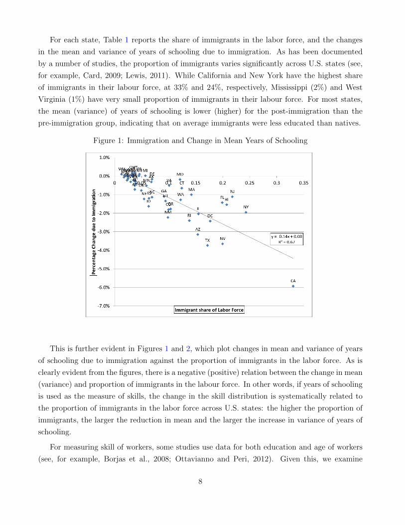
For each state, Table 1 reports the share of immigrants in the labor force, and the changes

in the mean and variance of years of schooling due to immigration. As has been documented

by a number of studies, the proportion of immigrants varies significantly across U.S. states (see,

for example, Card, 2009; Lewis, 2011). While California and New York have the highest share

of immigrants in their labour force, at 33% and 24%, respectively, Mississippi (2%) and West

Virginia (1%) have very small proportion of immigrants in their labour force. For most states,

the mean (variance) of years of schooling is lower (higher) for the post-immigration than the

pre-immigration group, indicating that on average immigrants were less educated than natives.

Figure 1: Immigration and Change in Mean Years of Schooling

This is further evident in Figures 1 and 2, which plot changes in mean and variance of years

of schooling due to immigration against the proportion of immigrants in the labor force. As is

clearly evident from the figures, there is a negative (positive) relation between the change in mean

(variance) and proportion of immigrants in the labour force. In other words, if years of schooling

is used as the measure of skills, the change in the skill distribution is systematically related to

the proportion of immigrants in the labor force across U.S. states: the higher the proportion of

immigrants, the larger the reduction in mean and the larger the increase in variance of years of

schooling.

For measuring skill of workers, some studies use data for both education and age of workers

(see, for example, Borjas et al., 2008; Ottavianno and Peri, 2012). Given this, we examine

8

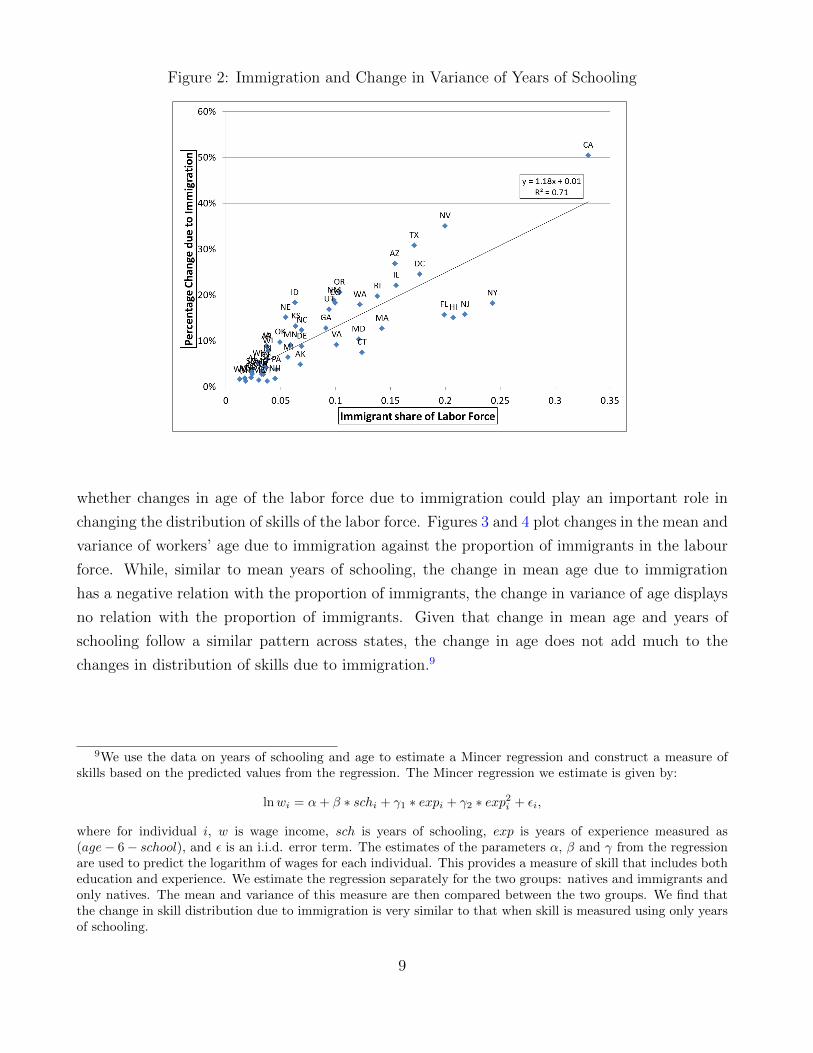
Figure 2: Immigration and Change in Variance of Years of Schooling

whether changes in age of the labor force due to immigration could play an important role in

changing the distribution of skills of the labor force. Figures 3 and 4 plot changes in the mean and

variance of workers’ age due to immigration against the proportion of immigrants in the labour

force. While, similar to mean years of schooling, the change in mean age due to immigration

has a negative relation with the proportion of immigrants, the change in variance of age displays

no relation with the proportion of immigrants. Given that change in mean age and years of

schooling follow a similar pattern across states, the change in age does not add much to the

changes in distribution of skills due to immigration.9

9We use the data on years of schooling and age to estimate a Mincer regression and construct a measure ofskills based on the predicted values from the regression. The Mincer regression we estimate is given by:

lnwi = α+ β ∗ schi + γ1 ∗ expi + γ2 ∗ exp2i + εi,

where for individual i, w is wage income, sch is years of schooling, exp is years of experience measured as(age− 6− school), and ε is an i.i.d. error term. The estimates of the parameters α, β and γ from the regressionare used to predict the logarithm of wages for each individual. This provides a measure of skill that includes botheducation and experience. We estimate the regression separately for the two groups: natives and immigrants andonly natives. The mean and variance of this measure are then compared between the two groups. We find thatthe change in skill distribution due to immigration is very similar to that when skill is measured using only yearsof schooling.

9

Figure 3: Immigration and Change in Mean Age

Figure 4: Immigration and Change in Variance of Age

10

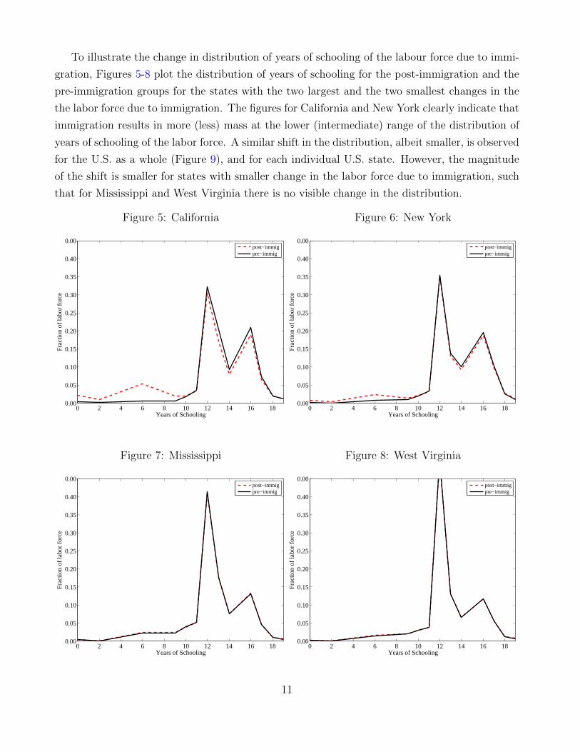
To illustrate the change in distribution of years of schooling of the labour force due to immi-

gration, Figures 5-8 plot the distribution of years of schooling for the post-immigration and the

pre-immigration groups for the states with the two largest and the two smallest changes in the

the labor force due to immigration. The figures for California and New York clearly indicate that

immigration results in more (less) mass at the lower (intermediate) range of the distribution of

years of schooling of the labor force. A similar shift in the distribution, albeit smaller, is observed

for the U.S. as a whole (Figure 9), and for each individual U.S. state. However, the magnitude

of the shift is smaller for states with smaller change in the labor force due to immigration, such

that for Mississippi and West Virginia there is no visible change in the distribution.

Figure 5: California

0 2 4 6 8 10 12 14 16 180.00

0.05

0.10

0.15

0.20

0.25

0.30

0.35

0.40

0.00

Years of Schooling

Fra

ctio

n of

labo

r fo

rce

post−immigpre−immig

Figure 6: New York

0 2 4 6 8 10 12 14 16 180.00

0.05

0.10

0.15

0.20

0.25

0.30

0.35

0.40

0.00

Years of Schooling

Fra

ctio

n of

labo

r fo

rce

post−immigpre−immig

Figure 7: Mississippi

0 2 4 6 8 10 12 14 16 180.00

0.05

0.10

0.15

0.20

0.25

0.30

0.35

0.40

0.00

Years of Schooling

Fra

ctio

n of

labo

r fo

rce

post−immigpre−immig

Figure 8: West Virginia

0 2 4 6 8 10 12 14 16 180.00

0.05

0.10

0.15

0.20

0.25

0.30

0.35

0.40

0.00

Years of Schooling

Fra

ctio

n of

labo

r fo

rce

post−immigpre−immig

11

Figure 9: United States

0 2 4 6 8 10 12 14 16 180.00

0.05

0.10

0.15

0.20

0.25

0.30

0.35

0.40

0.00

Years of Schooling

Fra

ctio

n of

labo

r fo

rce

post−immigpre−immig

In sum, the main effect of immigration on the skill distribution in each U.S. state is to shift the

distribution of years of schooling of the labor force: immigration increased the mass of workers at

the lower range of the distribution; and decreased the mass of workers for an intermediate range

of the distribution. We will use this observation to guide our theoretical analysis in Section 3

and for quantifying the effects of immigration on wages in Section 4.

3 The Model and its Predictions

We begin by considering the theoretical framework developed by Yeaple (2005). Consider an

economy with two sectors, X and Y , where X represents a composite differentiated product

and Y represents a homogenous good. Within each economy, the preferences of a representative

consumer are given by:

U = (1− β) lnY + β lnX

with

X =

(∫ N

0

x (i)σ−1σ di

) σσ−1

,

where there are N varieties of x, and σ is the elasticity of substitution between varieties of x.

This represents the standard setup of Dixit and Stiglitz (1977) with a preference for variety.

A continuum of workers with mass M populate the economy. Workers are heterogenous in

12

their skill level, Z; with higher Z, indicating a more skilled worker. There is a continuum of skill

levels, with the distribution of skills across all workers being given by G(Z), density by g(Z) and

support by [0,∞).

There exist two technologies that can be used to produce X, denoted by L and H, and one

technology to produce Y . Let φj(Z) represent the marginal product of a worker with skill level

Z, where j = Y, L,H denotes the technology that the worker is using. It is assumed that the

marginal product of all three technologies increase in Z, that is φ′j(Z) > 0; and that φj(0) = 1

for j = Y, L,H. In addition, it is assumed that marginal product of the three technologies satisfy

the following condition:

∂φH(Z)

∂Z

1

φH(Z)>∂φL(Z)

∂Z

1

φL(Z)>∂φY (Z)

∂Z

1

φY (Z)> 0. (1)

This assumption implies that, relative to all other workers, high skilled workers have a compara-

tive advantage in producing X with technology H; moderate skilled workers are assumed to have

a comparative advantage in producing X with technology L; and workers with the lowest skill

levels have a comparative advantage in producing Y . Figure 10 illustrates the marginal products

of labour for each different technology as functions of the skill level.10

Figure 10: Marginal product of labour as a function of skill level

Firms are ex-ante identical and can freely enter sector Y . Firms entering sector X produce

a single variety, and bear a technology specific fixed cost, Fj, with FH > FL. In the interest of

10For Figure 10, we assume the following functional forms for the marginal products for the three technologies:φY (Z) = Z2 + 1, φL (Z) = 2Z2 + 1 and φH (Z) = 3Z2 + 1.

13

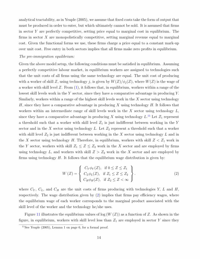
analytical tractability, as in Yeaple (2005), we assume that fixed costs take the form of output that

must be produced in order to enter, but which ultimately cannot be sold. It is assumed that firms

in sector Y are perfectly competitive, setting price equal to marginal cost in equilibrium. The

firms in sector X are monopolistically competitive, setting marginal revenue equal to marginal

cost. Given the functional forms we use, these firms charge a price equal to a constant mark-up

over unit cost. Free entry in both sectors implies that all firms make zero profits in equilibrium.

The pre-immigration equilibrium:

Given the above model setup, the following conditions must be satisfied in equilibrium. Assuming

a perfectly competitive labour market, in equilibrium workers are assigned to technologies such

that the unit costs of all firms using the same technology are equal. The unit cost of producing

with a worker of skill Z, using technology j, is given by W (Z)/φj(Z), where W (Z) is the wage of

a worker with skill level Z. From (1), it follows that, in equilibrium, workers within a range of the

lowest skill levels work in the Y sector, since they have a comparative advantage in producing Y.

Similarly, workers within a range of the highest skill levels work in the X sector using technology

H, since they have a comparative advantage in producing X using technology H. It follows that

workers within an intermediate range of skill levels work in the X sector using technology L,

since they have a comparative advantage in producing X using technology L.11 Let Z1 represent

a threshold such that a worker with skill level Z1 is just indifferent between working in the Y

sector and in the X sector using technology L. Let Z2 represent a threshold such that a worker

with skill level Z2 is just indifferent between working in the X sector using technology L and in

the X sector using technology H. Therefore, in equilibrium, workers with skill Z < Z1 work in

the Y sector, workers with skill Z1 ≤ Z ≤ Z2 work in the X sector and are employed by firms

using technology L, and workers with skill Z > Z2 work in the X sector and are employed by

firms using technology H. It follows that the equilibrium wage distribution is given by:

W (Z) =

CY φY (Z), if 0 ≤ Z ≤ Z1

CLφL(Z), if Z1 ≤ Z ≤ Z2

CHφH(Z), if Z2 ≤ Z <∞

. (2)

where CY , CL, and CH are the unit costs of firms producing with technologies Y, L and H,

respectively. The wage distribution given by (2) implies that firms pay efficiency wages, where

the equilibrium wage of each worker corresponds to the marginal product associated with the

skill level of the worker and the technology he/she uses.

Figure 11 illustrates the equilibrium values of log (W (Z)) as a function of Z. As shown in the

figure, in equilibrium, workers with skill level less than Z1 are employed in sector Y since they

11See Yeaple (2005), Lemma 1 on page 6, for a formal proof.

14

earn a higher wage in sector Y than in other sectors. Similarly, those with skill levels between

Z1 and Z2 are employed in sector X for firms using technology L, and those with skill levels

higher than Z2 are employed in sector X for firms using technology H. The slope of the wage

distribution is increasing at the thresholds, Z1 and Z2 because the value of an additional unit of

workers’ skill is greater for firms using the technologies that are progressively more sensitive to

skill.

Figure 11: Wage distribution

In what follows, it would be useful to determine the relative unit cost of production for each

technology. Let the price of Y, pY , be normalized to 1. Given that the Y sector is perfectly

competitive, we have CY = 1. Recall that, by definition, the threshold Z1 represents that skill

level for which workers are indifferent between working for a firm in sector Y and for a firm in

sector X using technology L. This, together with (2) , implies that

CL =φY (Z1)

φL(Z1)< 1. (3)

Similarly, Z2 represents the skill level for which workers are indifferent between working for a firm

in sector X using technology L, and for a firm in sector X using technology H, which together

15

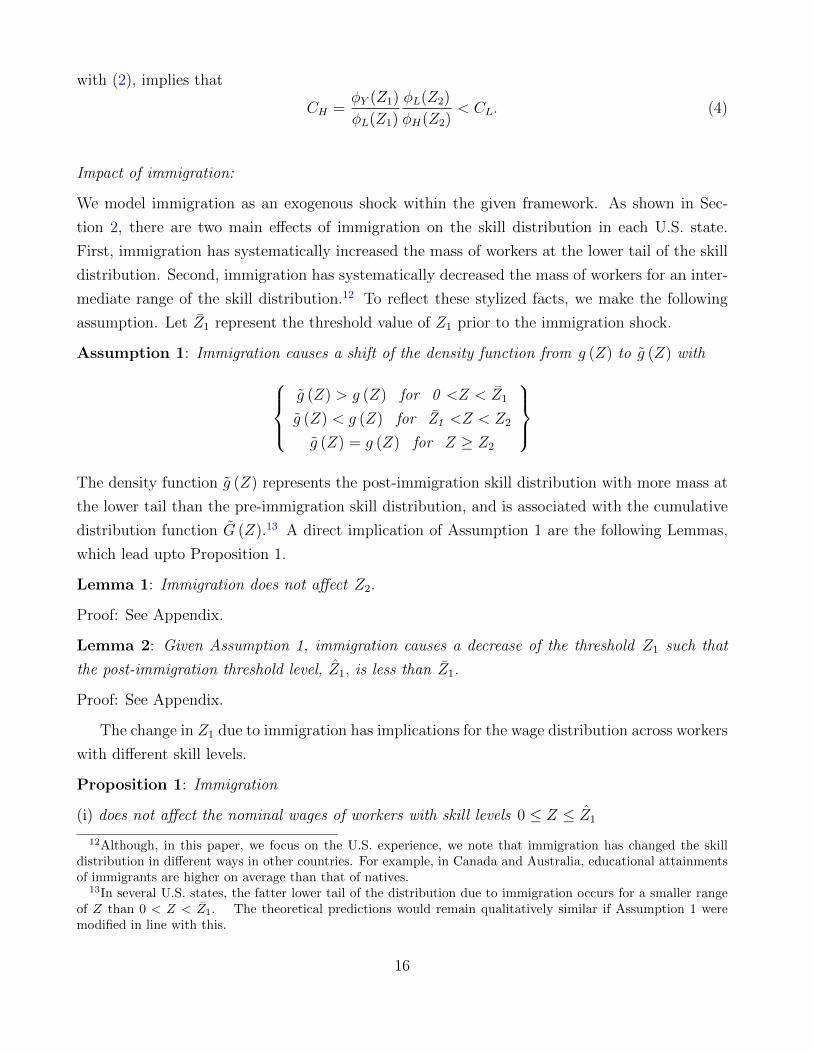
with (2), implies that

CH =φY (Z1)

φL(Z1)

φL(Z2)

φH(Z2)< CL. (4)

Impact of immigration:

We model immigration as an exogenous shock within the given framework. As shown in Sec-

tion 2, there are two main effects of immigration on the skill distribution in each U.S. state.

First, immigration has systematically increased the mass of workers at the lower tail of the skill

distribution. Second, immigration has systematically decreased the mass of workers for an inter-

mediate range of the skill distribution.12 To reflect these stylized facts, we make the following

assumption. Let Z1 represent the threshold value of Z1 prior to the immigration shock.

Assumption 1: Immigration causes a shift of the density function from g (Z) to g (Z) withg (Z) > g (Z) for 0 <Z < Z1

g (Z) < g (Z) for Z1 <Z < Z2

g (Z) = g (Z) for Z ≥ Z2

The density function g (Z) represents the post-immigration skill distribution with more mass at

the lower tail than the pre-immigration skill distribution, and is associated with the cumulative

distribution function G (Z).13 A direct implication of Assumption 1 are the following Lemmas,

which lead upto Proposition 1.

Lemma 1: Immigration does not affect Z2.

Proof: See Appendix.

Lemma 2: Given Assumption 1, immigration causes a decrease of the threshold Z1 such that

the post-immigration threshold level, Z1, is less than Z1.

Proof: See Appendix.

The change in Z1 due to immigration has implications for the wage distribution across workers

with different skill levels.

Proposition 1: Immigration

(i) does not affect the nominal wages of workers with skill levels 0 ≤ Z ≤ Z1

12Although, in this paper, we focus on the U.S. experience, we note that immigration has changed the skilldistribution in different ways in other countries. For example, in Canada and Australia, educational attainmentsof immigrants are higher on average than that of natives.

13In several U.S. states, the fatter lower tail of the distribution due to immigration occurs for a smaller rangeof Z than 0 < Z < Z1. The theoretical predictions would remain qualitatively similar if Assumption 1 weremodified in line with this.

16

(ii) increases the nominal wages of workers with skill Z > Z1.

Proof: Since CY = 1, and given that from (2) we have W (Z) = CY φY (Z) for 0 ≤ Z ≤ Z1, it

follows that immigration does not affect the wages of workers with skill levels 0 ≤ Z ≤ Z1. By

Lemma 2, Z1 decreases, implying that workers with skill levels Z1 ≤ Z ≤ Z1 switch from being

employed in sector Y to sector X, and earn higher wages since their marginal product rises due

to the switch. Moreover, post-immigration wages in sector X offered by firms using technology

L rise due to immigration. This is because, as Z1 decreases, from (1) and (3) , it follows that CL

increases, and from (2) , we have W (Z) = CLφL(Z). Thus, wages rise for all workers employed

by firms using technology L, including workers with skill levels Z1 ≤ Z ≤ Z2. Moreover, as Z1

decreases, from (1) and (4) , we have that CH increases. This corresponds to an increase in the

equilibrium wage of all workers with skill Z > Z2 �

Figure 12: Effect of immigration on the wage distribution

Figure 12 illustrates how the wage distribution is affected by immigration, as per Proposition

1. The intuition behind the Proposition is captured by the following three mechanisms:

1. ‘Entry effect’: Immigration raises the demand for final products across sectors, inducing

firm entry in each sector. Given that entry is more profitable in the monopolistically

competitive sector than the perfectly competitive sector, immigration raises the demand

for skilled workers relative to less-skilled workers and, thus, exerts an upward pressure on

17

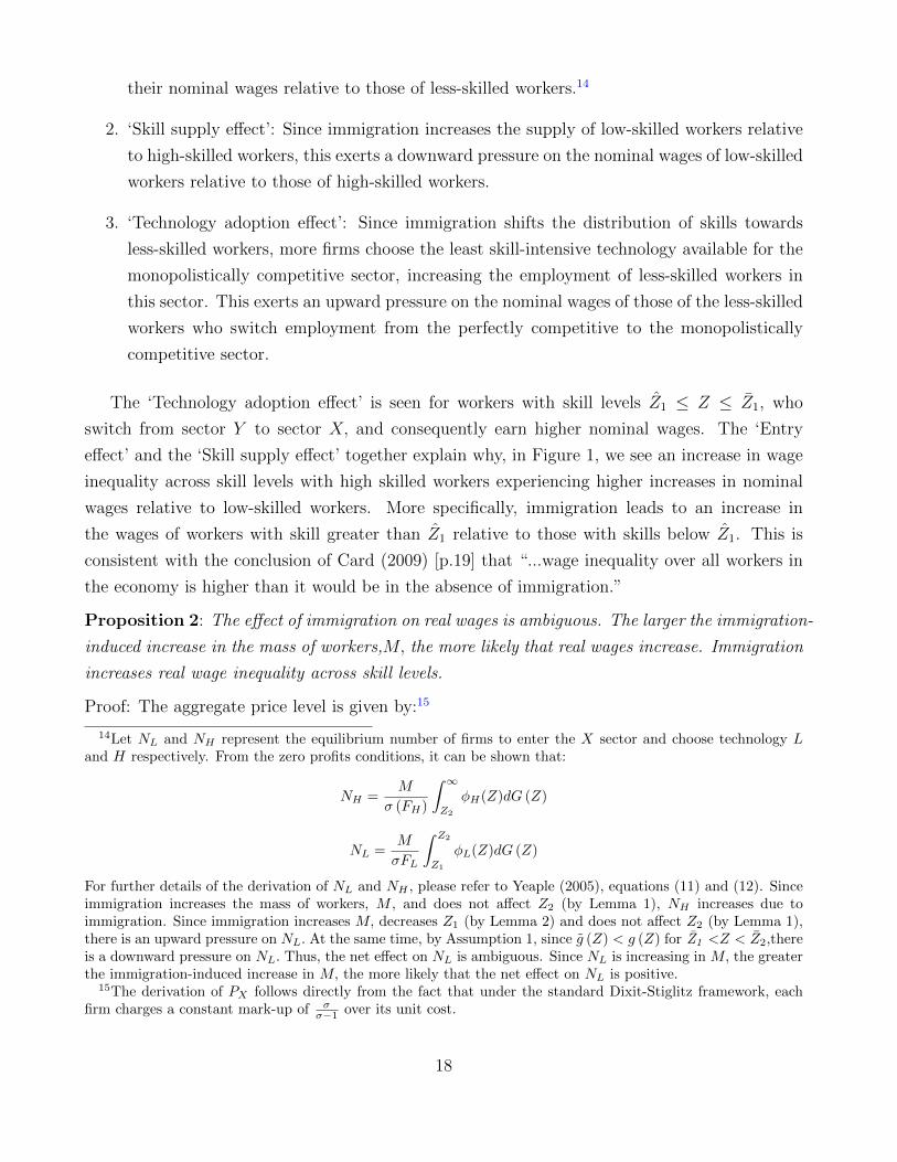
their nominal wages relative to those of less-skilled workers.14

2. ‘Skill supply effect’: Since immigration increases the supply of low-skilled workers relative

to high-skilled workers, this exerts a downward pressure on the nominal wages of low-skilled

workers relative to those of high-skilled workers.

3. ‘Technology adoption effect’: Since immigration shifts the distribution of skills towards

less-skilled workers, more firms choose the least skill-intensive technology available for the

monopolistically competitive sector, increasing the employment of less-skilled workers in

this sector. This exerts an upward pressure on the nominal wages of those of the less-skilled

workers who switch employment from the perfectly competitive to the monopolistically

competitive sector.

The ‘Technology adoption effect’ is seen for workers with skill levels Z1 ≤ Z ≤ Z1, who

switch from sector Y to sector X, and consequently earn higher nominal wages. The ‘Entry

effect’ and the ‘Skill supply effect’ together explain why, in Figure 1, we see an increase in wage

inequality across skill levels with high skilled workers experiencing higher increases in nominal

wages relative to low-skilled workers. More specifically, immigration leads to an increase in

the wages of workers with skill greater than Z1 relative to those with skills below Z1. This is

consistent with the conclusion of Card (2009) [p.19] that “...wage inequality over all workers in

the economy is higher than it would be in the absence of immigration.”

Proposition 2: The effect of immigration on real wages is ambiguous. The larger the immigration-

induced increase in the mass of workers,M, the more likely that real wages increase. Immigration

increases real wage inequality across skill levels.

Proof: The aggregate price level is given by:15

14Let NL and NH represent the equilibrium number of firms to enter the X sector and choose technology Land H respectively. From the zero profits conditions, it can be shown that:

NH =M

σ (FH)

∫ ∞Z2

φH(Z)dG (Z)

NL =M

σFL

∫ Z2

Z1

φL(Z)dG (Z)

For further details of the derivation of NL and NH , please refer to Yeaple (2005), equations (11) and (12). Sinceimmigration increases the mass of workers, M , and does not affect Z2 (by Lemma 1), NH increases due toimmigration. Since immigration increases M, decreases Z1 (by Lemma 2) and does not affect Z2 (by Lemma 1),there is an upward pressure on NL. At the same time, by Assumption 1, since g (Z) < g (Z) for Z1 <Z < Z2,thereis a downward pressure on NL. Thus, the net effect on NL is ambiguous. Since NL is increasing in M, the greaterthe immigration-induced increase in M, the more likely that the net effect on NL is positive.

15The derivation of PX follows directly from the fact that under the standard Dixit-Stiglitz framework, eachfirm charges a constant mark-up of σ

σ−1 over its unit cost.

18

PX =σ

σ − 1

(β

1− βM

σFL

) 11−σ

S (Z1)σσ−1

(∫ Z1

0

φY (Z) dG (Z)

) 11−σ

where

S (Z1)≡ φY (Z1)

φL(Z1)

From (1), it follows that S(Z1) is decreasing in Z1. The effect of immigration on PX is the net

result of the following effects. For σ > 1, immigration decreases PX by increasing M. Immigration

reduces Z1 from Z1 to Z1. This raises PX by increasing S (Z1) . The decrease in Z1 also decreases

the integral∫ Z1

0φY (Z) dG (Z) . At the same time, the increase in mass at the lower tail of the

skill distribution due to immigration increases the integral∫ Z1

0φY (Z) dG (Z) . Therefore, the

net effect on PX is ambiguous. This implies that net effect of immigration on real wages is

ambiguous. Since PX is decreasing in M, the greater the immigration-induced increase in M,

the more likely that the net effect on PX is negative, and, therefore, the more likely that the net

effect on real wages is positive. Since one of the implications of Proposition 1 is that nominal

wage inequality increases due to immigration, it follows that this applies also for real wages, since

the immigration-induced change in PX is applicable for all Z �

4 Impact of Immigration in U.S. states: Quantitative Re-

sults

We quantitatively evaluate the predictions of the model using the change in distribution of

education of workers due to immigration for U.S. states documented in Section 2. We determine

the effects of immigration-induced change in the distribution of skills of workers by comparing

the model predictions for nominal and real wages for natives only (pre-immigration) and natives

and immigrants (post-immigration) groups.

As for Figure 10, we assume the following functional forms for the marginal products for

the three technologies: φY (Z) = Z2 + 1, φL (Z) = 2Z2 + 1 and φH (Z) = 3Z2 + 1. These

functional forms are consistent with the condition for marginal products of technologies stated

in (1). Normalizing the size of a state for pre-immigration group to 1, we compute the size for the

post-immigration group as (1 + fraction of immigrants in the labor force). We assume β = 0.5,

which implies that, for the U.S. as a whole, individuals with high school education, or less, work

with the lowest skill intensive technology, Y . We assume σ = 4, which is consistent with estimates

19

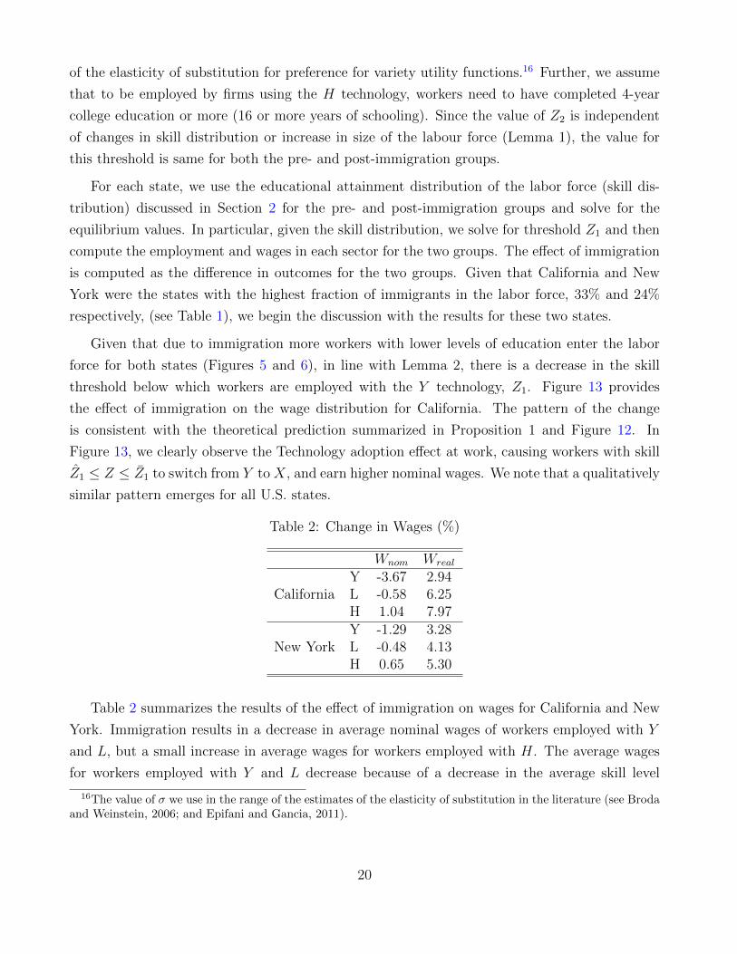
of the elasticity of substitution for preference for variety utility functions.16 Further, we assume

that to be employed by firms using the H technology, workers need to have completed 4-year

college education or more (16 or more years of schooling). Since the value of Z2 is independent

of changes in skill distribution or increase in size of the labour force (Lemma 1), the value for

this threshold is same for both the pre- and post-immigration groups.

For each state, we use the educational attainment distribution of the labor force (skill dis-

tribution) discussed in Section 2 for the pre- and post-immigration groups and solve for the

equilibrium values. In particular, given the skill distribution, we solve for threshold Z1 and then

compute the employment and wages in each sector for the two groups. The effect of immigration

is computed as the difference in outcomes for the two groups. Given that California and New

York were the states with the highest fraction of immigrants in the labor force, 33% and 24%

respectively, (see Table 1), we begin the discussion with the results for these two states.

Given that due to immigration more workers with lower levels of education enter the labor

force for both states (Figures 5 and 6), in line with Lemma 2, there is a decrease in the skill

threshold below which workers are employed with the Y technology, Z1. Figure 13 provides

the effect of immigration on the wage distribution for California. The pattern of the change

is consistent with the theoretical prediction summarized in Proposition 1 and Figure 12. In

Figure 13, we clearly observe the Technology adoption effect at work, causing workers with skill

Z1 ≤ Z ≤ Z1 to switch from Y to X, and earn higher nominal wages. We note that a qualitatively

similar pattern emerges for all U.S. states.

Table 2: Change in Wages (%)

Wnom Wreal

CaliforniaY -3.67 2.94L -0.58 6.25H 1.04 7.97

New YorkY -1.29 3.28L -0.48 4.13H 0.65 5.30

Table 2 summarizes the results of the effect of immigration on wages for California and New

York. Immigration results in a decrease in average nominal wages of workers employed with Y

and L, but a small increase in average wages for workers employed with H. The average wages

for workers employed with Y and L decrease because of a decrease in the average skill level

16The value of σ we use in the range of the estimates of the elasticity of substitution in the literature (see Brodaand Weinstein, 2006; and Epifani and Gancia, 2011).

20

Figure 13: Effect of immigration on wage distribution: California

0.5 0.55 0.6 0.65 0.70.2

0.25

0.3

0.35

0.4

0.45

0.5

Z1hat Z1bar Z2

of workers employed with these technologies.17 Thus, the Skill supply effect dominates for the

group of low-skilled workers on average. For the workers with the highest skill levels, on the

other hand, the Entry effect dominates, increasing their nominal wages. This is consistent with

Proposition 1 which implies that immigration of low skilled workers would result in an increase

in wage inequality.

To determine the change in real wages, we compute the difference in the price level between the

post-immigration and pre-immigration groups. Immigration results in a 6.42% (4.42%) decrease

in the aggregate price level in California (New York). This decrease in price level results in an

increase in real wages for workers in all sectors for both states.

Table 3: Change in Real Wages: Fixed Skill Levels (%)

Low Medium HighCalifornia 3.96 7.81 7.97New York 3.72 5.02 5.30

Given that skill distribution for each state determines the equilibrium threshold Z1 and that

immigration results in a change in Z1, change in average real wages for the three technologies are

not the appropriate comparison to the findings in the literature. To compare our results with

17In particular, even though wages of workers employed with the L technology increase, workers with lowerskill levels (who will have lower wages) are now employed with this technology. This would lower the averagenominal wage for the group.

21

the empirical findings in the literature we need to fix skill levels. Consistent with the definitions

in the literature (Borjas, 2003; Borjas et al., 2008; Card, 2009; Ottaviano and Peri, 2012, among

others), we define low skilled, Low, as workers with education level of high school or less, middle

skilled, Medium, as workers with some college and high skilled, High, as workers who have

complete university degrees. Using this definition we compute the change in the real wage for

low, medium and high skilled workers between the post-immigration and pre-immigration groups.

Table 3 provide the results for California and New York. Immigration results in an increase in

average real wages for all the three skill levels. In other words, whether we examine changes for

the three technologies or for fixed skill levels, immigration results in an increase in average real

wages for workers with the gains being higher for high skilled than low skilled workers. Therefore,

our findings are in line with evidence in Card (2009)which suggests that immigration to the U.S.

could result in an increase in wage inequality.

Figure 14: Change on Real Average Wages: Fixed Skill Levels

We summarize the effect of immigration on real wages of low, medium and high skilled

workers for all U.S. states in Figure 14. The figure plots the percentage change in average real

wage (difference between post- and pre-immigration) for the three skill levels and the fraction of

immigrants in the labor force for each state. With the exception of low skilled workers in Kansas,

North Carolina and South Dakota, average real wages are higher for the post-immigration group

than the pre-immigration group for all skill levels in all states. The figure also illustrates that

22

the difference in average real wages between the two groups are 1) lower for low skilled workers

than medium and high skilled workers; and 2) positively related to the fraction of immigrants in

the labor force. In sum, similar to the findings for California and New York, immigration results

in an increase in wage inequality in all states, with the increase being higher for states with a

higher fraction of immigrants in the labor force.

4.1 Robustness

We examine the robustness of our quantitative findings by relaxing some of the assumptions

made for computing the effects of immigration on wages.

4.1.1 Trade and Labor mobility

We assumed that the U.S. states are in autarky (prices differ across states) and that there is

no mobility of labor between states (wages differ across states). We relax these assumptions by

computing the effect of immigration using the change in skill distribution due to immigration for

the U.S. as a whole (Figure 9), which would imply integrated goods and labor markets for the

whole of U.S. In other words, through mobility of goods and/or labor across states, the effects

of immigration to U.S. states would be transmitted to the whole country. Table 4 summarizes

the results for the change in average wages for the three skill levels. Given that the fraction of

immigrants in the labor force for the U.S. is lower than that for California and New York, the

effects are smaller than those for the two states.18 However, the pattern for the change is similar:

average real wages for all three skill levels for the post-immigration group are higher than for

the pre-immigration group, with the difference being higher for medium than for the low skilled

workers and highest for the high skilled workers.

Table 4: Change in Wages: United States (%)

Wnom Wreal

Low -0.81 1.95Medium 0.03 2.81High 0.30 3.09

18The percentage immigrants in the labor force for the U.S. is 15% compared to 33% for California and 24%for New York.

23

4.1.2 Sensitivity of Results: Parameter Values

We evaluate the sensitivity of our quantitative findings to using other values for the parameters

β, the consumption share of X goods, and σ, the elasticity of substitution for varieties of X. For

California, Table 5 provides the change in average real wages for low skilled workers and price

level for different values of β. As β increases, the consumption share for good Y decreases, which

reduces the threshold Z1 as fewer workers are demanded in the Y sector. Increasing the value

of β results in smaller reduction in the price level and a lower increase in average real wages for

low skilled workers.

Table 5: Sensitivity of Results to Value of β: California

β Low Wreal Price0.40 4.63 0.930.45 4.68 0.930.50 3.96 0.940.55 3.25 0.940.60 1.67 0.96

Table 6 provides the change in average real wages for low skilled workers and price level for

different values of σ for California. The value of σ only affects the price level and hence the

change in nominal wage is the same as before. As σ increases, that is the differentiated goods

become more substitutable, the reduction in price level due to immigration is lower, which implies

a smaller increase in average real wages of low skilled workers

Table 6: Sensitivity of Results to Value of σ: California

σ Low Wreal Price

3 8.33 0.904 3.96 0.945 1.99 0.95

5 Conclusion

We document that the main effect of immigration on the skill distribution in each U.S. state is

to increase the mass of workers at the lower range of the distribution and reduce the mass for

an intermediate range of the skill distribution. We use this systematic pattern to analyze the

effect of immigration of low skilled workers using a model that allows for firms to endogenously

24

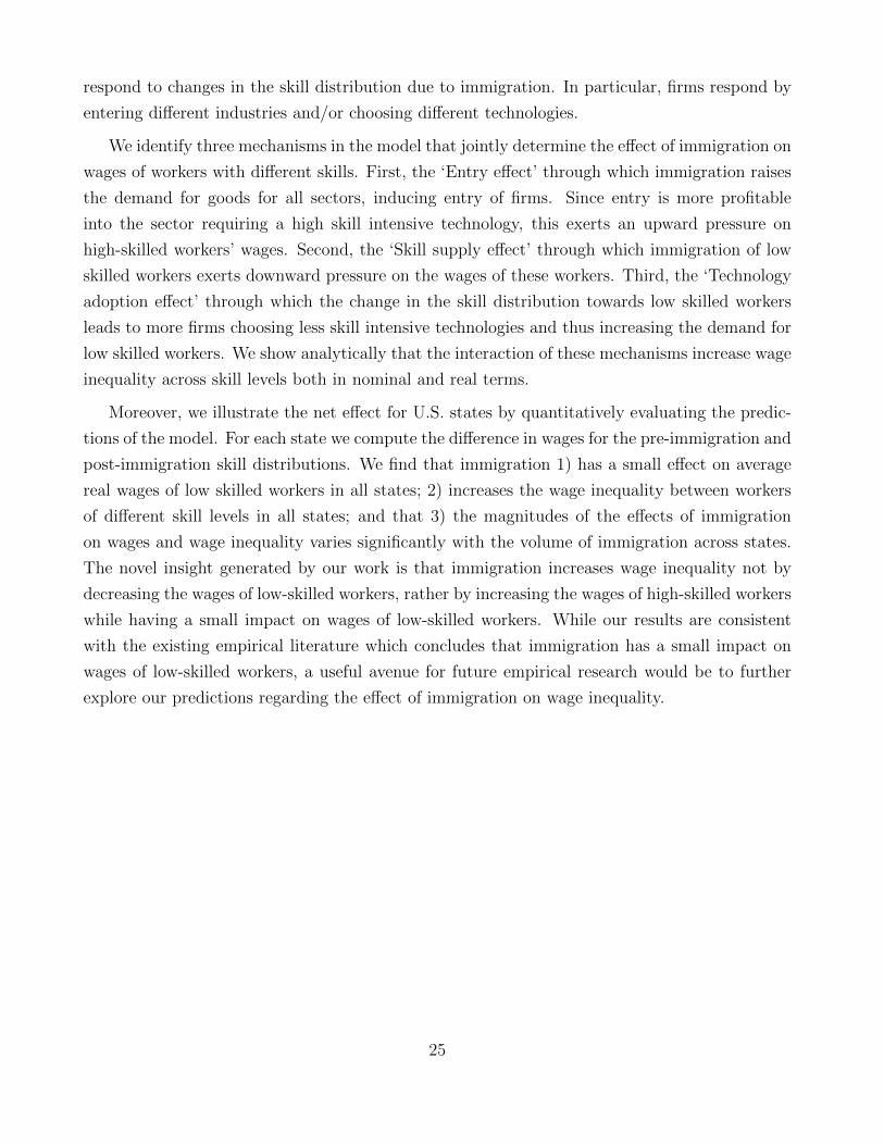
respond to changes in the skill distribution due to immigration. In particular, firms respond by

entering different industries and/or choosing different technologies.

We identify three mechanisms in the model that jointly determine the effect of immigration on

wages of workers with different skills. First, the ‘Entry effect’ through which immigration raises

the demand for goods for all sectors, inducing entry of firms. Since entry is more profitable

into the sector requiring a high skill intensive technology, this exerts an upward pressure on

high-skilled workers’ wages. Second, the ‘Skill supply effect’ through which immigration of low

skilled workers exerts downward pressure on the wages of these workers. Third, the ‘Technology

adoption effect’ through which the change in the skill distribution towards low skilled workers

leads to more firms choosing less skill intensive technologies and thus increasing the demand for

low skilled workers. We show analytically that the interaction of these mechanisms increase wage

inequality across skill levels both in nominal and real terms.

Moreover, we illustrate the net effect for U.S. states by quantitatively evaluating the predic-

tions of the model. For each state we compute the difference in wages for the pre-immigration and

post-immigration skill distributions. We find that immigration 1) has a small effect on average

real wages of low skilled workers in all states; 2) increases the wage inequality between workers

of different skill levels in all states; and that 3) the magnitudes of the effects of immigration

on wages and wage inequality varies significantly with the volume of immigration across states.

The novel insight generated by our work is that immigration increases wage inequality not by

decreasing the wages of low-skilled workers, rather by increasing the wages of high-skilled workers

while having a small impact on wages of low-skilled workers. While our results are consistent

with the existing empirical literature which concludes that immigration has a small impact on

wages of low-skilled workers, a useful avenue for future empirical research would be to further

explore our predictions regarding the effect of immigration on wage inequality.

25

Appendix:

Proof of Lemma 1:

The equilibrium value of the threshold Z2 is derived from the zero profit condition. Under the

standard monopolistic competition model, due to free entry, firms in sector X make zero profits

in equilibrium. Therefore, the revenues of firms using either H or L technologies must exactly

equal their costs. Given preferences characterized by constant elasticity of substitution (CES),

the revenue of a firm using technology j less its variable costs is a fixed multiple of its revenue,

which, in turn, given free entry, must be less than or equal to its fixed cost. Moreover, under

the standard Dixit-Stiglitz framework, firms using technology j ∈ {L,H} realize revenues of Rj,

where

Rj =(βEP σ−1

X

)p1−σj (5)

with PX representing the aggregate price of all varieties of X, and

pj =σ

1− σCj (6)

representing the price of the individual variety j. Together, (5) and (6) imply that

RH

RL

=

(CHCL

)1−σ

If both L and H technology firms make zero profits then equating revenues to fixed costs provides

the following condition: (CHCL

)1−σ

=CHFHCLFL

Using (3) and (4), this implies that, in equilibrium, Z2 must satisfy the following equation:

φL (Z2)

φH (Z2)=

(FHFL

)− 1σ

(7)

Since immigration does not affect the parameters FH , FL, and σ, or the functions φL (Z) and

φH (Z) , we have that Z2 is unaffected by immigration. �

Proof of Lemma 2:

The equilibrium value of the threshold Z1 is derived from the market clearing condition of sector

Y, that is, total expenditure on Y must equal the total income generated in sector Y . Expenditure

on Y is given by:

Y = (1− β)E = (1− β)MW. (8)

26

Given Cobb-Douglas preferences, the expenditure on Y must equal (1− β)E, where E is total

expenditure, M is the mass of workers, and W , the average wage, is given by:

W ≡∫ Z1

0

φY (Z) dG (Z) + CL

∫ Z2

Z1

φL (Z) dG (Z) + CH

∫ ∞Z2

φH (Z) dG (Z) . (9)

For the market of Y to clear, (8) must equal the total income generated in sector Y, as given

by M∫ Z1

0φY (Z) dG (Z). For a given value of Z2, this implies that in equilibrium Z1 must satisfy:

β

1− β1

S (Z1)

∫ Z1

0

φY (Z) dG (Z) =

∫ Z2

Z1

φL (Z) dG (Z) + A (Z2)

∫ ∞Z2

φH (Z) dG (Z) , (10)

where CL = S (Z1) ≡ φY (Z1)φL(Z1)

, with S(Z1) decreasing in Z1.

Assumption 1 implies that holding constant the value of Z1 at Z1, immigration causes an

increase in the value of the left hand side of (10) from∫ Z1

0φY (Z) dG (Z) to

∫ Z1

0φY (Z) dG (Z).

Also, holding constant the value of Z1 at Z1, immigration causes a decrease in the value of the

right hand side of (10) from∫ Z2

Z1φL (Z) dG (Z) to

∫ Z2

Z1φL (Z) dG (Z). Given that Z2 is unaffected

by immgration, in order for (10) to be satisfied post-immigration, we must have that Z1 decreases

to a level below Z1, since 1S(Z1)

∫ Z1

0φY (Z) dG (Z) is increasing in Z1 �

27

References

Blau, F.D. and L.M. Kahn (2012) “Immigration and the distribution of incomes.” NationalBureau of Economic Research, Working Paper No. 18515, Cambridge, MA.

Bowen, H.P. and J.P. Wu (2012) “Immigrant specificity and the relationship between tradeand immigration: theory and evidence.” McColl School of Business, Discussion Paper No. 2011-01.

Borjas, G. J. (2003) “The labor demand curve is downward sloping: Reexamining the impactof immigration on the labor market.” The Quarterly Journal of Economics, 118(4), 1335-1374.

Borjas, G. J., R.B. Freeman and L.F. Katz (1997) “How do much do immigration and tradeaffect labor market outcomes?” Brookings Papers on Economic Activity, 1-90.

Borjas, G. J., J. Grogger, and G. Hanson (2008). “Imperfect Substitution between Immigrantsand Natives: A Reappraisal.” National Bureau of Economic Research, Working Paper No. 13887,Cambridge, MA.

Broda, C. and Weinstein, D. E. (2006) “Globalization and the Gains from Variety.” TheQuarterly Journal of Economics, 121(2), 541-585.

Card, D. (2001) “Immigrant Inflows, Native Outflows, and the Local Labor Market Impactsof Higher Immigration.” Journal of Labor Economics 19(1): 22-64.

Card, D. (2007) “How Immigration Affects U.S. Cities.” CReAM Discussion Paper No 11/07.

Card, D. (2009) “Immigration and inequality.” American Economic Review, 99(2), 1-21.

Card, D. (2012) “Comment: The elusive search for negative wage impacts of immigration.”Journal of the European Economic Association, 10(1), 211-215.

Card, D. and E.G. Lewis (2007) “The Diffusion of Mexican Immigrants during the 1990s.”In Mexican Immigration to the United States, University of Chicago Press: 193-277.

Cortes, P. (2008) “The effect of low-skilled immigration on US prices: evidence from CPIdata.” Journal of Political Economy, 116(3), 381-422.

Dixit, A. and Stiglitz, J. (1977) “Monopolistic competition and optimum product diversity.”American Economic Review, 67(3), 297-308.

Epifani, P. and Gancia, G. (2011) “Trade, markup heterogeneity and misallocations.” Journalof International Economics, 83(1), 1-13.

Gaston, N. and D.R. Nelson (2013) “Bridging trade theory and labour econometrics: Theeffects of international migration.” Journal of Economic Surveys 27(1): 98-139.

Kerr, S.P. and W.R. Kerr (2011) “Economic impacts of immigration: A survey.” NBERWorking Paper No. w16736.

Lewis, E.G. (2005) ”The Impact of Immigration on New Technology Adoption in US Manu-facturing.” Federal Reserve Bank of Philadelphia.

Lewis, E.G. (2008) “How did the Miami labor market absorb the Mariel immigrants?” FederalReserve Bank of Philadelphia Working Paper No. 04–3.

Lewis, E.G. (2011) “Immigration, Skill Mix, and Capital Skill Complementarity.” The Quar-

28

terly Journal of Economics, 126(2), 1029-1069.

Manacorda, M., A. Manning and J. Wadsworth (2012) “The impact of immigration on thestructure of male wages: Theory and evidence for Britain.” Journal of the European EconomicAssociation 10(1), 120-151.

Organization for Economic Cooperation and Development (OECD)(2011) “International Mi-gration and the SOPEMI.”

Ottaviano, G. I. P. and G. Peri (2012) “Rethinking the effects of immigration on wages.”Journal of the European Economic Association 10(1), 152-197

Peri, G. (2012) “The Effect Of Immigration On Productivity: Evidence From US States.”The Review of Economics and Statistics, 94(1), 348-358.

Yeaple, S. (2005) “A simple model of firm heterogeneity, international trade, and wages.”Journal of International Economics, 65(1), 1-20.

29