Embed Size (px)
Citation preview
Tilburg University
Essays on network formation and exchange
Dogan, G.
Publication date:2009
Link to publication in Tilburg University Research Portal
Citation for published version (APA):Dogan, G. (2009). Essays on network formation and exchange. [s.n.].
General rightsCopyright and moral rights for the publications made accessible in the public portal are retained by the authors and/or other copyright ownersand it is a condition of accessing publications that users recognise and abide by the legal requirements associated with these rights.
• Users may download and print one copy of any publication from the public portal for the purpose of private study or research. • You may not further distribute the material or use it for any profit-making activity or commercial gain • You may freely distribute the URL identifying the publication in the public portal
Take down policyIf you believe that this document breaches copyright please contact us providing details, and we will remove access to the work immediatelyand investigate your claim.
Download date: 17. Dec. 2021

Essays on Network Formation and Exchange
Gönül Doğan Ligtvoet

ISBN/EAN: 978-90-5335-216-8
Essays on Network Formation and Exchange
Proefschrift ter verkrijging van de graad van doctor aan de Universiteit van Tilburg, op gezag van de rector magnificus, prof.dr. Ph. Eijlander, in het openbaar te verdedigen ten overstaan van een door het college voor promoties aangewezen commissie in de aula van de Universiteit op
vrijdag 30 oktober 2009 om 14.15 uur
door
Gönül Doğan Ligtvoet
geboren op 28 januari 1979 te Bursa, Turkije.

Promotores: Prof.dr. J.J.M. Potters Prof.dr. K. Sijtsma
Copromotor: Dr. M.A.L.M. van Assen

Acknowledgements
Her gün bir yerden göçmek ne iyi
Her gün bir yere konmak ne güzel
Bulanmadan, donmadan akmak ne hoş
Dünle beraber gitti cancağızım
Ne kadar söz varsa düne ait
Şimdi yeni şeyler söylemek lazım
Mevlânâ Celâleddin-i Rûmî
This thesis is the result of an interdisciplinary project. I started the project with
the knowledge that I needed to investigate social networks, but I soon realised
that it is a huge field of study. Sociologists have been studying networks for
decades, and economists were keen on catching up in the last 15 years. (Now I
know that physicists, psychologists and computer scientists are also working on
networks.) At first, I had trouble in even understanding sociology papers but then
I learned how to benefit from them with the right approach. I learned how to
write scientific papers and endlessly revise them. Sometimes I was so consumed
with the idea of networks that I started seeing networks in everything. New ideas
on social networks and social preferences sprung up along the way; some excite
me and I hope to pursue further.
Both of my supervisors, Jan Potters and Marcel van Assen, provided me with
valuable feedback and insights into how to think like a scientist. I would like to
thank them for their time and effort during this project. I would also like to
thank the committee members of this thesis (Charles Noussair, Klaas Sijtsma,
Michael Kosfeld, Theo Offerman, and Vincent Buskens) for their valuable
comments. Thanks to Ton Heinen for providing me with the facilities after my
contract ended; I would not be able to finish my last paper otherwise. Thanks to
Marieke Timmermans for her secretarial support.
My experience during the four and a half years of my PhD taught me that every
PhD comes with a unique story. And mine is not an exception. Despite all the
struggles I had -especially in the last months before finishing- and no real
encouragement, I persevered. So, it is not only finishing the thesis but knowing
that I successfully endured this process that makes this thesis a great
achievement. Moreover, knowing that I can now build my own research agenda

and be independent is a relief. I am grateful for the help of my friends and
family here and elsewhere for providing me with the necessary support
throughout.
I would like to thank:
Carmen for all our talk over everything; Anne-Kathrin for having minimal but
effective conversations in the last couple of months; Wilco and Wobbe for always
asking how things are; Anna for the occasional dinners; Owen for the frisbee and
somehow making me feel not strange during my job search and Maria-Cristina for
the yoga.
Mercan, we have süp-per dreams that we still have to work on. Rahmi, it is good
to have a friend who cares and does not care at the same time. Serap, Erdem,
Ulaş, Pelin, Umut and Zeynep; it is always nice seeing you.
Special thanks to Josep. The former Londoner and the new Parisien. Or the
Catalan or the Spaniard. You are a great friend and I hope you keep that way.
Darja, Matthias, and Miriam; my London trips would be incomplete without
seeing you.
Annem Gülhas Doğan ve babam Süleyman Doğan’a sınırsız desteklerinden dolayı;
Đlhan ve Fatma’ya bütün Đstanbul ve Kaş seyahatlari için; yeni gelen Selim Mert’e
varolduğu için; kuzenim Semra’ya her zaman yanımda olduğu için teşekkürü
özellikle borç bilirim.
Ik wil de familie Ligtvoet (Sjannie, Ger, Leslie, en Cindy) ook bedanken voor de
zorg over mij, voor de goede lachen en of course het lenen van de auto.
And Rudy. The prince, the ginger, sweeto and pō-ta-tō, the object of some of my
nightmares, hayatım benim, canım beniiim, the rolling r that I cannot pronounce,
the dedicated and the I-forgot. Thanks for all, but we are just beginning.
As the great poet and mystic Mevlana, better known as Rumi in English, says
above, yesterday has passed and now is the time to say new things.
Gönül Doğan Ligtvoet
31 Ağustos.August.Augustus 2009, Tilburg

Contents
1. Introduction……………………………………………………….……………….………….1
2. Coordination in a 3-Player Network Formation Game
2.1. Introduction ………………………………….……………….........…………………...7
2.2. The Game ……………………………………….…………………………………………11
2.3. Experimental Design ……………………….……………………........…………….21
2.4. Results …………………………………………….………………………….……………23
2.4.1. Link Formation Results ………….………………………….……………23
2.4.2. Coordination Strategies of the Buyers ……….………….…………..30
2.4.3. Coordination Strategies of the Seller ………….………….………….33
2.4.4. Link Formation Results at the Group Level ….………….………..36
2.5. Discussion and Conclusion …………………………………….………….……….41
Appendix 2A. List of Networks ……………………………………….…………...…….45
Appendix 2B. Experimental Instructions for the Cost-40 Treatment. ….…47
Appendix 2C. Tables ………………………………………………………………….…..….51
3. The Effect of Link Costs on the Formation and Outcome of Buyer-
Seller Networks
3.1. Introduction………………………………………………………………….……………55
3.2. The Game……………………………………………………………………….………….60
3.3. Experimental Design……………………………………………………….………….67
3.4. Results…………………………………………………………………………….…………70
3.5. Discussion……………………………………………………………………….…………80
3.6. Conclusion……………………………………………………………………….…………84
Appendix 3A. Experimental Instructions for the Cost-0 Treatment........… 87
4. Stability of Exchange Networks
4.1. Introduction………………………………………………………….……………….……97
4.2. Theoretical Background………………………………………….…………………...99
4.3. Definitions of Stability, Equality, Efficiency.…………….…………………..103
4.4. Results………………………………………………………………….…………………..106
4.5. Discussion…………………………………………………………….……………………116
Appendix 4A. Expected Value Theory…………………………….….…………………121
5. Testing Models of Pure Exchange
5.1. Introduction……………………………………………………………..………………..125
5.2. Models and Hypotheses………………………….…………………..……………….128
5.3. Michener et al.’s Experiments……………………………………...……………….137
5.4. Results…………………………………………………………………………………….….141
5.5. Discussion………………………………...……………………………….……………..…147
5.6. Conclusion…………………………………………………….…………………………....151
Appendix 5A. Experimental Results and Theories’ Predictions of Final
Allocations………………………………………………………………………………………….154
Appendix 5B. Michener et al.’s Experiments and Coleman’s Model…….……160
6. Conclusions……………………………………………………….……………………….……161
References…………………………………………………………….………………………..…….169
Samenvatting in Nederlands……………………………….………………………..…….179

Chapter 1
Introduction
Exchange of goods, and services as well as ideas, favors, and gifts constitutes a
basic part of human existence. Exchange has been extensively studied in economics
since the pioneering work of Edgeworth (1881). In social psychology and sociology,
research on exchange gained a prominent position after Homans (1958) introduced
the idea of social behavior as exchange.
In many real life situations, agents need to establish or maintain a connection to
engage in exchange. Examples include the labor market, housing market,
friendships, and collaborations among scientists. In the labor market, the potential
employee and the employer first establish a connection via an application process
before the job is negotiated. Likewise in the housing market, registering with a
housing agency is a prerequisite for a potential tenant to start seeing the available
houses. We tend to exchange gifts and favors only with our friends, and family.
Scientists can exchange ideas and collaborate only if they are connected to each
other.
Often, setting up or maintaining a connection (i.e., a link) is costly, and agents
establish or keep their connections only if it is of benefit to them. So, the set of links
agents have (i.e., the network) might play an important role in determining the
outcomes of exchange. Who can interact with whom affects not only the potential
gains from exchange but also how the gains are distributed. Typically, agents with
more links and trading opportunities are in a better bargaining position than more
isolated agents. Therefore the study of exchange cannot be parted from the set of
connections among agents. Nonetheless, not until the work of Myerson (1977) in
economics, and the works of Stolte and Emerson (1977) and Cook and Emerson
(1978) in sociology the set of links that agents need to establish or maintain has
been taken into account in the study of exchange. The recent but rapidly growing
body of theoretical literature in economics shows that networks affect the outcomes
of interactions (for an overview see e.g., Goyal, 2007; Jackson, 2008). Moreover, in
sociology, the main result of predominantly empirical research on networks is that
1

network structure has a large impact on what actors earn in their relations (e.g., see
Carrington, Scott, and Wasserman, 2005 for a recent review; Willer, 1999).
Agents’ payoffs depend on their position in the network, and this dependence
provides an incentive for agents to change the network structure. So, not every
network structure can be expected to be resistant to change, i.e., not every network
is stable. Similarly, some network structures might lead to inefficiencies in
exchanges. The study of stable and efficient networks is central to the study of
social networks in economics. In various network formation models, link costs play
a prominent role in determining the set of stable and efficient networks. For
example, in the buyer-seller networks model of Kranton and Minehart (2001)
minimally connected networks are both efficient and stable in a range of link costs.
Unlike in economics, in sociology almost all the theoretical and empirical studies
on exchange focused on the effect of a given network structure on the outcomes of
persons on different positions (see Breiger, Carley, and Pattison, 2003 for an
overview on work on “dynamic” network studies in sociology). The stability or
efficiency of networks was not until recently the subject of investigation in
sociological research on networks (see Buskens and Van de Rijt, 2008a, for an
exception).
The theoretical literature on network formation in economics has not yet been
matched with much empirical and experimental work. There have been only a
handful of studies that experimentally investigate the predictions of some network
formation models. (See Berninghaus, Ehrhart, and Ott, 2006; Berninghaus,
Ehrhart, Ott, and Vogt, 2007; Callander and Plott, 2005; Deck and Johnson, 2004;
Falk and Kosfeld, 2003; Goeree, Riedl, and Ule, 2008). In this thesis, we contribute
to the network formation literature in economics in two ways. In the first paper, we
use experiments to analyze the strategies of the players in a repeated network
formation game. The repeated game setup makes it possible for some players to
anti-coordinate their actions such that by doing the opposite actions and turn-
taking they reach a better outcome than in the one-shot game. It is also possible for
a third player to facilitate coordination that benefits other players. We thus
investigate the coordination behavior of the players and how it is affected by the
2
link costs. There are only a few studies on anti-coordination in which players do the
opposite actions and take turns in order to maximize their payoff in a repeated
setting (see Erev and Haruvy, 2008; Helbing, Schönhof, Stark, and Holyst, 2005;
Kaplan and Ruffle, 2008). Most of the previous studies on network formation
mainly focused on whether players coordinate on forming the star or cycle
networks. In these network formation experiments being linked was generally
better than not being linked. Unlike the previous anti-coordination and network
formation experiments, in our study we focus both on the coordination and anti-
coordination behaviors of players. Also, in our network formation game whether
some players benefit from forming a link depends on the links of other players. The
second contribution of this thesis is the analysis of behavior in a game with both
network formation and interaction over the network. Almost all the previous
network formation experiments assumed an exogenous structure of payoffs. There
are only a few studies that studied the interaction over an exogenously given
network (e.g. Charness, Corominas-Bosch, and Fréchette, 2007; Judd and Kearns,
2008). To our knowledge, the second paper of this thesis is among the first1 to
study both network formation and interaction over the network in the experimental
network literature. In this study, players first decide whether to form a link or links
and then bargain over a surplus if they are linked. This study allows us to test the
assumption that sunk link costs do not affect the subsequent bargaining in the
links.
This thesis does not only contribute to the economics literature on network
formation, bargaining, and coordination, but also to the sociological literature on
network formation and exchange. The theoretical literature on network formation
in sociology largely focused on the effect of adding and deleting links on the payoffs
of the players in the network without analyzing the stability or efficiency of a given
network. (See e.g. Leik, 1991, 1992; Van Assen and Van de Rijt, 2007; Willer and
Willer, 2000). The third paper of this thesis contributes to the sociology literature
on networks by studying the stability and efficiency of exchange networks. In this
1 Corbae and Duffy (2008) also studied a two-stage network game in which players first decided with whom to form links and then played the coordination game.
3

paper, different from the previous studies, we focus on results on the stability and
efficiency of networks of any size, and characterize all the stable networks up to size
eight as well as the efficient and egalitarian networks with varying link costs using a
model of exchange in the sociological literature. Finally, in the fourth paper of this
thesis we explain experimental outcomes in pure exchange situations while
focusing on the efficiency of exchange. The comparison of the predictions of
various models from economics and sociology to the data from pure exchange
experiments sheds new light on how well these models explain exchange behavior
in the laboratory. We also provide insights into the behavioral patterns observed in
the experimental results that cannot be predicted by the models considered.
This thesis contains four substantive chapters. Each chapter is based on a separate
paper including an introduction to the topic and relevant literature, outline of the
theoretical predictions, and presentation and discussion of the results. The first two
papers present two different experiments, and thus, also include information on
the experimental design. The experimental instructions, some tables and further
explanations on some procedures are included in the appendices of the relevant
chapters. The last chapter of the thesis concludes.
In Chapter 2 we experimentally examine the impact of the link costs on network
formation and coordination in a repeated buyer-seller network formation game.
Particularly, we investigate whether two buyers and a seller coordinate on forming
the non-competitive networks. The repeated play of the game allows for the
equilibrium in which the long side of the market, i.e. the buyers, anti-coordinate
their actions and take turns to maximize their payoff. However, as is shown in the
paper, there is also an equilibrium in which the seller facilitates coordination that
maximizes the buyers’ payoff. Thus, the repeated link formation game lets us
investigate whether the players coordinate, and who facilitates the coordination.
We also study whether link costs affect the network formation and coordination
behavior. We find that the link costs do not significantly affect the link offers of
players. Regardless of the link costs, there exist evidence for coordination on the
non-competitive networks facilitated both by the short side and the long side of the
market. The coordination behavior is further reflected by the group level results.
4
Notably, the majority of the groups play similar to the coordination equilibria
regardless of the link costs. However, contrary to what one might expect, link costs
do not increase the number of coordinating groups.
Chapter 3 is an experimental investigation of the impact of the link costs on
network formation and the ensuing bargaining process in a buyer-seller setting. In
our game, two buyers and one seller can form either a competitive or a non-
competitive network, and then bargain over the surplus given that they have a link.
We examine the occurrence of competitive networks in which the seller is predicted
to get the entire surplus, and analyze whether the bargaining process in the
network is affected by the link costs. Standard theory predicts that link costs lead to
less competitive networks, but that there is no effect of link costs on the bargaining
outcomes within the network because the costs are sunk. We find support for the
first but not the second prediction. So, link costs not only cause significantly fewer
competitive networks to be formed, but also conditional on the type of the network,
link costs have a significant impact on the bargaining outcomes. Specifically, link
costs do not affect the bargaining outcome in the competitive network but increase
the bargaining share of the buyer in the non-competitive network. Hence our study
falsifies the assumption that bargaining is independent of the link costs incurred
earlier. Moreover, as we show in the chapter, such an effect of link costs on the
bargaining outcomes constitutes a major puzzle that cannot be completely
explained by inequality aversion, equity theory, or loss aversion.
In Chapter 4, we investigate which network structures emerge as a function of link
costs if actors choose with whom to maintain links. We focus on stable networks
and investigate whether they are socially efficient, Pareto efficient and egalitarian.
First, we show that, under some mild assumptions the minimal networks consisting
of dyads are socially efficient and stable for a range of link costs regardless of how
the payoffs are distributed. Second, we calculate the payoff distributions of all
networks up to size eight, and analyze the stable networks with varying link costs
by using the expected value theory proposed by Friedkin (1995) in the sociological
literature on exchange networks. We find that only a very small number of
networks are stable. In even-sized networks, minimal networks are the only
5

egalitarian, Pareto efficient, socially efficient, and stable networks over a wide
range of link costs. In odd-sized networks, cycles are the most prominent
egalitarian and stable networks. These cycles are also Pareto efficient, although
they are not socially efficient. We also find that at low link costs social dilemmas
exist such that no even-sized network exists that is both stable and Pareto efficient.
The existence of social dilemmas suggests that agents can establish a network
structure in which they are not willing to change their links but that is Pareto
dominated by another network that is not stable.
Chapter 5 explains human behavior in pure exchange situations. We reanalyze the
experimental data of Michener, Cohen, and Sørenson (1975, 1977) and compare the
data to the predictions of various cooperative bargaining models from economics,
and to the predictions of a bilateral exchange model adapted from sociology.
Specifically, we consider the cooperative bargaining solutions of Nash (1950),
Raiffa-Kalai-Smorodinsky (Kalai & Smorodinsky, 1975; Raiffa, 1953), Myerson
(1977), and the bilateral exchange model of Stokman and Van Oosten (1994). We
find that the bilateral exchange model fits the exchange data better than all the
other models considered. However, systematic deviations from predictions of the
bilateral exchange model and other models of rational behavior are observed. Such
deviations can be explained by a boundedly rational model of exchange assuming
that actors use heuristics with different sophistication levels to detect profitable
exchange. In line with the predictions of the bounded rationality model, we find
that the exchange opportunities that require more sophistication are less likely to
be carried out. Models that assume rationality fail to predict the results of exchange
if agents need to give up a good they like most to increase their payoff.
Finally, Chapter 6 summarizes the findings of the previous chapters, and then
discusses their contribution to the network formation and exchange literatures. We
also put forward some ideas for future work.
6

Chapter 2
Coordination in a 3-Player Network Formation Game∗∗∗∗
2.1. Introduction
In many markets buyers and sellers need to establish or have connections with each
other to be able to engage in trade. Such connections (i.e., links) between the
buyers and the sellers in a market, and the structure of these connections (i.e., the
network) have been the subject of a rapidly growing interest in economics. Various
theoretical models identified the effect of the shape of the buyer-seller networks on
the payoffs of agents (see Corominas-Bosch, 2004; Kranton and Minehart, 2000;
and Wang and Watts, 2006). In these models, typically, agents with more links and
trading opportunities get a better share of the surplus than more isolated agents.
Also, link costs affect the links that are formed among the agents. Despite the sharp
predictions of the theoretical models, there have been only a few studies that
investigate buyer-seller networks in the laboratory (see Charness et al. 2007; Gale
and Kariv, 2008; Judd and Kearns, 2008). These studies focused on a fixed
network structure, and analyzed the effect of the network structure on agents’
payoffs. In general, in these experiments it was found that agents with fewer links
attain lower payoffs. Note, however, that the formation of the network was not
studied in these experiments.
The present paper contributes to the experimental literature on networks by
studying the formation of networks. We focus on coordination behaviour in a
finitely repeated network formation game. In this game, if the long side of the
market competes, the short side of the market gets the entire surplus. Moreover,
competition leads to negative payoffs for the competing parties if they incur costs
for getting the opportunity to trade. However, if the long side of the market anti-
coordinates their actions such that only one player enters into trade with the short
side, then that one player earns positive payoffs. Since positive earnings for the
long side of the market are only possible by anti-coordination, in the one-shot
∗ This chapter is based on Doğan (2009), unpublished manuscript.
7
game, it is not obvious who enters into trade and who stays out. Such a problem,
however, can be solved if the game is repeated. It is possible for the agents in the
long side of the market to enter into trade in turns (anti-coordination), or the short
side of the market can trade with one agent at a time (coordination) if the long side
punishes deviations. Whether agents engage in anti-coordination or coordination,
and how link costs affect their behaviour are the main questions investigated in this
paper.
We focus on the simplest buyer-seller network formation game in which
coordination strategies of players in a repeated game can be investigated. There is
one seller who has one good and two potential buyers. All the players
simultaneously make link offers; the seller decides whether to form a link with one
buyer or two buyers and the buyers decide whether to form a link with the seller. If
a competitive network is formed in which the seller is linked to both buyers, then
the entire surplus goes to the seller. If the seller is linked to one buyer only, the
surplus is shared, albeit not equally, between the seller and the linked buyer. In this
non-competitive network, the seller earns two-thirds of the surplus, and the linked
buyer one-third. In the one-shot game, offering two links is a weakly dominating
strategy for the seller regardless of the link costs. It is a weakly dominating strategy
for the buyers to offer a link to the seller only if the links are costless. So, playing
the undominated one-shot game strategies results in the formation of the
competitive network in every period if the links are costless. If the links are costly,
however, the competitive network can not be supported as an equilibrium of the
repeated game. Hence, link costs are predicted to reduce the occurrence of
competitive networks. In a repeated game, there are other equilibria which ensure
that the buyers maximize their total payoff while maintaining equality among each
other. We focus on two repeated game equilibria that lead to such outcomes. First,
it is possible for the buyers to anti-coordinate their link offers so as to form one link
in an alternating fashion every period. Such anti-coordination constitutes a
subgame perfect equilibrium regardless of the link costs. Second, instead of
offering two links every period, the seller can coordinate on forming one link if the
8
buyers punish deviations by the seller2. This equilibrium, as we will show in this
paper, also holds regardless of the link costs. We thus investigate whether players
engage in coordination, if so who facilitates the coordination, and whether
coordination is affected by the link costs.
There exist two strands of experimental literature related to this paper. The first is
the study of anti-coordination in the finitely repeated games of chicken, battle of
the sexes, entry, and congestion. Similar to our study, in these games if the game is
repeated, then agents can do the opposite actions and take turns to maximize their
joint payoffs while also maintaining equality. Such anti-coordination behaviours
did not receive substantial attention in the experimental literature, and the
evidence for anti-coordination was mixed3. Rapoport, Guyer and Gordon (1976)
studied a variant of the chicken game in a repeated setting and found anti-
coordination to be prevalent. Similarly, Arifovic, McKelvey, and Pevnitskaya
(2006) showed that players anti-coordinated in the repeated battle of the sexes
games. Helbing et al. (2005) studied what they called the 2-persons congestion
game. In this game choosing the Pareto dominating action yielded zero payoff for
both players whereas alternating their actions maximized their long-run payoff.
They found that the players often learned to alternate their actions in the repeated
game. There was no conclusive evidence for alternation behaviour in repeated
market entry games (see Erev and Haruvy, 2009 for an overview; Kaplan and
Ruffle 2008). Unlike all these studies that exclusively studied anti-coordination, in
our setting both coordination and anti-coordination is possible. The buyers can
anti-coordinate and take turns on the non-competitive network, but taking turns on
the non-competitive network can also be facilitated by the seller. Moreover, the
2 For the sake of simplicity, in the rest of this paper, we will mostly stick to the expressions
“coordinating on one link” for both buyer anti-coordination and seller coordination
behaviour, “buyer coordination” to refer to the buyer anti-coordination, and “seller
coordination” to refer to the seller coordination.
3 Anti-coordination behaviour received little attention also in the theoretical network
literature. There exist two theoretical papers that investigate anti-coordination in networks
by Bramoullé (2007), and Bramoullé, Lopez-Pintado, Goyal, and Vega-Redondo (2004).
9

network formation game makes it possible for us to study the anti-coordination
behaviour of players also when a weakly dominating strategy exists in the one-shot
game4. The existence of a weakly dominating strategy might make anti-
coordination more difficult to achieve.
The second strand of related experimental literature focuses on network formation
and examines whether behaviour in link formation games is in line with the
predictions of various theoretical models (See Berninghaus et al., 2006, and 2007;
Callander and Plott, 2005; Deck and Johnson, 2004; Falk and Kosfeld, 2003;
Goeree, Riedl, and Ule, 2008). In most of these papers the focus was on whether
certain network structures such as “stars” and “cycles”, which were predicted to be
formed by the considered theoretical model, emerged in the laboratory. Attaining
those structures posed a coordination problem for the players involved. In all these
studies, being linked almost always led to higher payoffs than not being linked. The
coordination results of these studies were mixed. Coordination on a star structure
mostly failed if players were homogenous as in Goeree et al (2008) or if the player
who payed for the link was not the sole beneficiary of the link as in Falk and
Kosfeld (2003). However, players mostly formed the star structures in the
continuous time setting of Berninghaus et al (2006, 2007), and with heterogeneous
agents of Goeree et al (2008). Also, in both Falk and Kosfeld (2003), and Callander
and Plott (2005) coordination on the cycle network occurred in the majority of the
cases. Different from these network formation studies, in our game, not all the
players have similar incentives for forming a certain network. Whereas the seller is
better off in a competitive network, the buyers are better off by anti-coordinating
on the non-competitive network. Moreover in a repeated setting, the buyers can
induce the seller to coordinate on forming the non-competitive network by
punishing deviations.
In this paper, we first show that formation of the non-competitive network with
alternating buyers constitutes an equilibrium of the finitely repeated game, and
such a formation can be facilitated either by buyer anti-coordination, or seller
4 If the link costs are 0.
10

coordination behaviour. Our experimental results show that the link costs do not
significantly affect the seller or the buyers’ link offers, and there exist both buyer
and seller coordination in both cost treatments. The coordination behaviour is
further reflected at the group level results that show that regardless of the link
costs, the majority of the groups play similar to coordination equilibria. Among the
coordinating groups, some engage in the buyer coordination, some in the seller
coordination, and some in both. Interestingly, the number of coordinating groups
does not increase with the link costs.
The remainder of this paper is organized as follows. The next section presents the
game along with the hypotheses that are derived from the equilibrium analysis.
Section 2.3 outlines the experimental design and procedure. Section 2.4 presents
the experimental results and tests of the various hypotheses. Section 2.5 discusses
and concludes.
2.2. The Game
The game involves one seller and two buyers. The players simultaneously offer
links to each other. The two buyers cannot form a link with each other. Links can
be considered as necessary connections for trade to take place. Since trade requires
the consent of both players, a link is formed when both players offer it. After the
simultaneous link offer stage, the payoffs are realised according to the link or links
that are formed, and the next period starts. We investigate two cases with differing
link costs. In the first case, links are costless; in the second, each link that is formed
costs 40 points. The cost of a link can be thought of as a necessary investment for
trade to take place. The cost of a link is the same for both sellers and buyers. Costs
are incurred once a link is formed, not when a link is offered. The link offers of the
players are made common knowledge at the end of the link formation.
There are 16 different networks that can be formed considering the link offers of
the seller and the buyers. We categorize these 16 networks according to the number
of links formed, and for simplicity call them the no-link networks, 1-link networks,
and the 2-link network. In the no-link networks no player has a link. Nine networks
11
are categorized as no-link networks. In the 1-link networks one buyer maintains a
link with the seller. Six networks are categorized as 1-link networks. In the 2-link
network both buyers have a link with the seller. The 16 networks are depicted in the
Appendix 2A in Figure 2A.1.
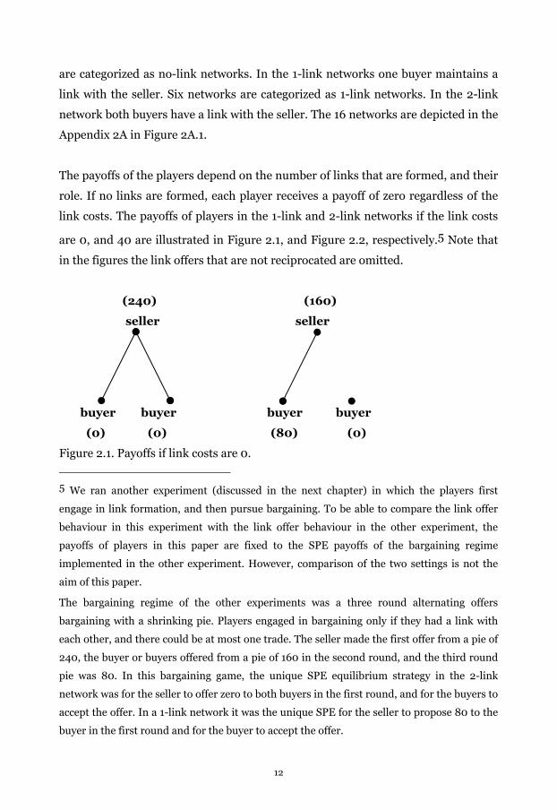
The payoffs of the players depend on the number of links that are formed, and their
role. If no links are formed, each player receives a payoff of zero regardless of the
link costs. The payoffs of players in the 1-link and 2-link networks if the link costs
are 0, and 40 are illustrated in Figure 2.1, and Figure 2.2, respectively.5 Note that
in the figures the link offers that are not reciprocated are omitted.
(240) (160)
seller seller
buyer buyer buyer buyer
(0) (0) (80) (0)
Figure 2.1. Payoffs if link costs are 0.
5 We ran another experiment (discussed in the next chapter) in which the players first
engage in link formation, and then pursue bargaining. To be able to compare the link offer
behaviour in this experiment with the link offer behaviour in the other experiment, the
payoffs of players in this paper are fixed to the SPE payoffs of the bargaining regime
implemented in the other experiment. However, comparison of the two settings is not the
aim of this paper.
The bargaining regime of the other experiments was a three round alternating offers
bargaining with a shrinking pie. Players engaged in bargaining only if they had a link with
each other, and there could be at most one trade. The seller made the first offer from a pie of
240, the buyer or buyers offered from a pie of 160 in the second round, and the third round
pie was 80. In this bargaining game, the unique SPE equilibrium strategy in the 2-link
network was for the seller to offer zero to both buyers in the first round, and for the buyers to
accept the offer. In a 1-link network it was the unique SPE for the seller to propose 80 to the
buyer in the first round and for the buyer to accept the offer.
12
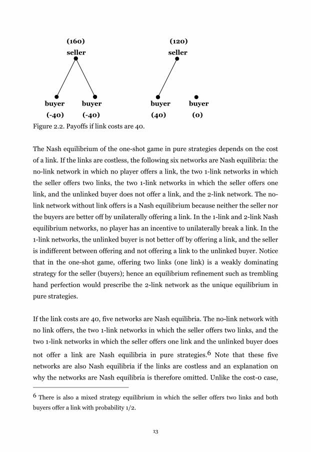
(160) (120)
seller seller
buyer buyer buyer buyer
(-40) (-40) (40) (0)
Figure 2.2. Payoffs if link costs are 40.
The Nash equilibrium of the one-shot game in pure strategies depends on the cost
of a link. If the links are costless, the following six networks are Nash equilibria: the
no-link network in which no player offers a link, the two 1-link networks in which
the seller offers two links, the two 1-link networks in which the seller offers one
link, and the unlinked buyer does not offer a link, and the 2-link network. The no-
link network without link offers is a Nash equilibrium because neither the seller nor
the buyers are better off by unilaterally offering a link. In the 1-link and 2-link Nash
equilibrium networks, no player has an incentive to unilaterally break a link. In the
1-link networks, the unlinked buyer is not better off by offering a link, and the seller
is indifferent between offering and not offering a link to the unlinked buyer. Notice
that in the one-shot game, offering two links (one link) is a weakly dominating
strategy for the seller (buyers); hence an equilibrium refinement such as trembling
hand perfection would prescribe the 2-link network as the unique equilibrium in
pure strategies.
If the link costs are 40, five networks are Nash equilibria. The no-link network with
no link offers, the two 1-link networks in which the seller offers two links, and the
two 1-link networks in which the seller offers one link and the unlinked buyer does
not offer a link are Nash equilibria in pure strategies.6 Note that these five
networks are also Nash equilibria if the links are costless and an explanation on
why the networks are Nash equilibria is therefore omitted. Unlike the cost-0 case,
6 There is also a mixed strategy equilibrium in which the seller offers two links and both
buyers offer a link with probability 1/2.
13
the 2-link network is not a Nash equilibrium because a buyer has an incentive to
unilaterally delete the link with the seller, which improves her payoffs from –40 to
0. In the one-shot game, offering two links is a weakly dominating strategy for the
seller if the link costs are 40, so the only trembling hand perfect equilibria in pure
strategies are the two 1-link networks in which the seller offers two links.
The repeated game admits multiple pure strategy Nash equilibria as well as
multiple subgame perfect Nash equilibria (SPE). Assuming that the players do not
discount the future7, any combination of the Nash equilibria of the one-shot game
throughout the experiment is a SPE equilibrium of the repeated game. To
characterize all the SPE of the repeated game is complicated, and is beyond the
scope of this paper. For a detailed exposition of the Nash and SPE equilibria of
repeated games see Vega-Redondo (2003; Chapter 8).
In this paper we focus our analysis on three types of play: repeated play of the
undominated strategies of the one-stage game and the two repeated game
strategies that require coordinating on the formation of a 1-link network in each
period. All three strategies can be supported as a SPE of the repeated game
regardless of the link costs.
As the experimental literature points out, players generally avoid playing
dominated strategies8. Hence we investigate the repeated play of the undominated
strategies in this game. In the one-shot game, it is a weakly dominating strategy for
the seller to offer two links regardless of the link costs. For the buyers, it is a weakly
7 The design of the experiment implicitly assumes that players do not discount the future
such that the payoffs of the players are constant across periods.
8 For example, in the dominance solvable beauty contest games of Nagel (1995), few subjects
chose the weakly dominated strategies. Similar results were found in the two-iteration
dominance-solvable symmetric normal-form games of Stahl and Wilson (1994, 1995), and in
the two- and three- iteration dominance solvable games of Costa-Gomes, Crawford, and
Broseta (2001). Notice that in the network formation game considered in this paper, there is
only one step of iteration needed for playing the undominated strategy.
14

dominating strategy to offer a link each only if the link costs are 0. There does not
exist a weakly dominating strategy for the buyers if the link costs are 40. So, the
repeated play of the undominated strategies predicts a 2-link network to be formed
in every period if the link costs are 0. If the link costs are 40, however, the repeated
formation of 2-link networks cannot be supported as an equilibrium. The growing
social preference literature has shown that inequality aversion is not uncommon
among players. So, we analyzed the two repeated game strategies that yield less
unequal payoffs for the buyers compared to the undominated strategy play but
require coordination among the players. These two strategies result in the
formation of a 1-link network in each period with an alternating buyer so that not
only the total payoff of the buyers is maximal but also the buyers’ earnings are the
same. Hence each buyer has an incentive to sustain these strategies. These two
strategies differ in who coordinates the formation of the 1-link network; in the first
it is the buyers (buyer coordination) and in the second it is the seller (seller
coordination) who alternates the link offer. In the buyer coordination strategy, the
seller offers two links every period, and buyers alternate in forming a link with the
seller by taking turns in offering a link. In the seller coordination strategy, the
buyers offer a link each to the seller every period, and the seller offers a link to one
buyer only in an alternating fashion. We first prove that these two repeated game
strategies are indeed equilibria.
Proposition 1. Buyer Coordination: Regardless of the link costs, in the
repeated game, the following strategies can be supported as a SPE: the seller offers
two links in every period, and the buyers alternate in offering a link to the seller.
Proof: We know that playing a stage Nash equilibrium in each period is a repeated
game SPE. So, the 1-link network in which the seller offers two links, and the
buyers offer a link in alternating periods is also a SPE of the repeated game
regardless of the link costs. Q.E.D.
Notice that in the buyer coordination equilibrium, it is assumed that both the seller
and the buyers stick to the equilibrium play if they are indifferent. For example, in
the cost-0 case if the seller offers two links in every period, and buyer 1 offers a link
in the odd-numbered periods, then it is also a SPE that buyer 2 offers a link in all
15

periods. Nonetheless, it can be shown that the buyer coordination equilibrium can
be sustained as a strict equilibrium via appropriate punishment structures.
The next proposition shows how the seller coordination strategy can be supported
as a SPE of the repeated game with an appropriate punishment structure.
Proposition 2. Seller Coordination: Regardless of the link costs, until the last
three periods of the repeated game the following strategies can be supported as a
SPE: buyers offer a link each in every period, and the seller alternates in offering a
link to the buyers.
Proof: Without loss of generality assume that both buyers offer a link to the seller,
and the seller offers a link to buyer 1 at odd numbered periods, and to buyer 2 at
even numbered periods. Now, assuming that the seller and buyer 2 stick to the
equilibrium play in every period, buyer 1 does not deviate in an odd numbered
period because she is worse off by deviating. The same argument holds for buyer 2
in even numbered periods. Buyer 1 (2) does not deviate in even (odd) numbered
periods, because she is not better off by deviating9. However, the seller has an
incentive to deviate in every period because if she offers two links she earns more;
i.e. 240 instead of 160 in cost-0 case, and 160 instead of 120 in the cost-40 case. So,
to prevent the seller from offering two links at any period a punishment strategy is
necessary.
If the seller deviates from equilibrium play and offers two links in a period, then
both buyers offer no link for at least one period as a punishment (seller punishment
hereafter). Notice that with this punishment structure the seller is strictly worse off
by deviating: she earns 240 (160) in the deviation period and zero for the
punishment period instead of earning 160×2 (120×2) for two periods if the link 9 As in the buyer coordination equilibrium, SPE assumes that if the players are indifferent
between two actions, then they stick to the equilibrium play. The following punishment
structure rules out such indifference: if say buyer 1 deviates in an even numbered period,
then the seller offers two links for two consecutive periods, and buyer 2 offers a link whereas
buyer 1 does not offer a link. Any deviation by buyer 1 from the punishment repeats the
punishment.
16
costs are 0 (40). Now, a buyer prefers to deviate and form a link with the seller
instead of punishing the seller. So, the following is necessary to sustain the
punishment of the seller (buyer punishment hereafter). If buyer 1 deviates from not
offering a link in the seller punishment, then buyer 2 offers a link to the seller for at
least two consecutive periods, the seller offers two links in these two periods. Buyer
1 does not offer a link in these two periods. Any deviation by buyer 1 in the buyer
punishment phase repeats the punishment. So, assume buyer 1 deviates in the
seller punishment period, then she earns 80 (40) in the deviation period and zero
in the next two periods if the link costs are 0 (40). If buyer 1 does not deviate from
the seller punishment, then she earns zero for one period, and 80 (40) in total in
the next two periods if the link costs are 0 (40). So buyer 1 is not better off by
deviating from punishing the seller. Buyer 2, on the other hand, is strictly better off
by punishing buyer 1; buyer 2 earns 80×2 (40×2) if she punishes buyer 1, and 80
(40) if she does not punish buyer 1 if the link costs are 0 (40). The seller is
indifferent between punishing and not punishing buyer 1, and earns 160×2 (120×2)
if the link costs are 0 (40). So, a minimum of three periods are necessary to sustain
the equilibrium. In the last three periods any one-stage Nash equilibrium can be
played. Q.E.D.
The next proposition provides the networks that cannot be supported as a SPE of
the repeated game with any punishment structure.
Proposition 3. Regardless of the link costs, strategies leading to the repeated
formation of no-link networks in which there is at least one link offer cannot be
supported as a SPE of the repeated game. If the link costs are 40, strategies leading
to the repeated formation of 2-link networks can also not be supported as a SPE of
the repeated game.
Proof. In the eight no-link networks with at least one link offer, all players earn
their minmax payoff10 such that assuming that the players best-respond, any 10 Formally, the minmax payoff is defined as the min max g ( , )
i j i i ia A a A i i ia a− ≠∈× ∈ − where ai
є Ai is player i’s pure action, iji Aa ≠− ×∈ is any combination of pure actions of players other
than i, and gi is player i’s payoff function.
17
combination of actions by other players cannot lower their payoff. Since there is at
least one link offer by one player in these no-link networks, there exists a one
period profitable deviation for at least one player. The player who is offered a link is
better off by deviating and offering a link to that player. Such a deviation cannot be
punished because players cannot be made worse off than their minmax payoff.
Similarly, if link costs are 40, in the 2-link network, both buyers prefer to deviate
by not forming a link and such a deviation cannot be punished. Q.E.D.
To sum up, the repeated play of all one-stage Nash equilibrium networks can be
supported as a repeated game SPE. We focus on the buyer coordination
equilibrium in which a 1-link network is formed every period, the seller offers two
links every period, and the buyers alternate their link offers. We also show that the
repeated play of some networks which are not one-stage Nash equilibria can be
supported as repeated SPE. Among such networks, we give emphasis to the seller
coordination equilibrium in which the buyers always offer two links and the seller
alternates her link offer every period. Finally, there exist networks whose repeated
play cannot be supported as a SPE of the repeated game.
Hypotheses
We formulate the theoretical predictions into five hypotheses. The first and the
second hypotheses are based on the play of undominated strategies of the stage
game. The third hypothesis is on the link formation in a coordination equilibrium.
The fourth and the fifth hypotheses are on the buyers’ and seller’s link offers
assuming the buyer and the seller coordination, respectively.
Link Formation in Undominated Strategies of the One-Shot Game
1. The 2-link network is formed less often if the link costs are 40 than if the
link costs are 0.
If both the seller and the buyers play the weakly dominating strategies of
the one-shot game, then a 2-link network is formed at all periods if the link
costs are 0. If the seller plays the weakly dominating strategy of the one-
18

shot game, i.e., offers two links, then in equilibrium a 1-link network is
formed at all periods if the link costs are 40.
Link Offers in Undominated Strategies of the One-Shot Game
2.1. Link costs do not affect the seller’s link offer.
Offering two links is a weakly dominating strategy for the seller in the one-
shot game irrespective of the link costs.
2.2. The buyers are less likely to offer a link if the link costs are 40 than if the
link costs are 0.
Offering a link is a weakly dominating strategy for both buyers in the one-
shot game if the link costs are 0 but not if the link costs are 40.
Link Formation in a Coordination Equilibrium
3. Regardless of the cost treatment, the conditional probability that a link is
formed with buyer 1 (2) given that a link is formed with buyer 2 (1) is
smaller than the marginal probability that a link is formed with buyer 1
(2).
In a buyer or seller coordination equilibrium one link is formed with
alternating buyers in each period. So, the probability of having a 1-link
network is not independent of the probability of buyer 1 or buyer 2 having a
link. If we define 1PrlinkBuyer as the probability that buyer 1 forms a link, and
1 2Pr |linkBuyer Buyer as the probability that buyer 1 forms a link given that buyer
2 forms a link, then by dependence of the link formation process the
following holds in a coordination equilibrium:
1 1 2Pr Pr |link linkBuyer Buyer Buyer> and 2 2 1Pr Pr |link link
Buyer Buyer Buyer> .
Link Offers in a Buyer Coordination
4. Regardless of the cost treatment, the conditional probability that buyer 1
(2) offers a link given that buyer 2 (1) offers a link is smaller than the
marginal probability that buyer 1 (2) offers a link.
19
In a buyer coordination equilibrium, the buyers alternate on offering a link
to the seller, and the seller offers two links regardless of the link costs. So,
the link offer decisions of the buyers are not independent of each other. If
we define 1Prlink offer
Buyer as buyer 1’s probability of offering a link, and
2
1Pr |
Buyer
link offerBuyer as the probability that buyer 1 offers a link given that
buyer 2 offers a link, then by dependence of the link offers the following
holds in a buyer coordination:
2
1 1Pr Pr |
Buyer
link offer link offerBuyer Buyer> and
1
2 2Pr Pr |
Buyer
link offer link offerBuyer Buyer> .
Link Offers in a Seller Coordination
5. Regardless of the cost treatment, the conditional probability that the
seller offers a link to buyer 1 (2) given that she offers a link to buyer 2 (1)
is smaller than the marginal probability the seller offers a link to buyer
1(2).
In a seller coordination equilibrium, the seller offers one link to the buyers
in an alternating fashion, and the buyers offer two links regardless of the
link costs. So, the seller’s link offer decision to a particular buyer is not
independent of her link offer decision to the other buyer. If we define
1Prlink offer
Seller as the seller’s probability of offering a link to buyer 1, and
2
1Pr |
Seller
link offerSeller as the seller’s probability of offering a link to buyer 1
given that she offers a link to buyer 2, then the dependence of the link
offers of the seller implies the following in a seller coordination:
2
1 1Pr Pr |
Seller
link offer link offerSeller Seller> and
1
2 2Pr Pr |
Seller
link offer link offerSeller Seller> .
Notice that the hypotheses are not mutually exclusive. The undominated strategy
play predicts the formation of the 1-link network if the link costs are 40 but does
not prescribe which 1-link network is formed. Also, the last two hypotheses can be
confirmed for the same group if both the buyers and the seller coordinate on
forming one link.
20

2.3. Experimental Design
The experiments were conducted at the CentERlab in Tilburg University, the
Netherlands. A total of 63 subjects participated in 4 sessions, and each subject
participated only once. Subjects were recruited through email lists of students
interested in participating in experiments. There were in total 30 subjects (10
groups) in 2 sessions in the cost-0 treatment, and 33 subjects (11 groups) in 2
sessions in the cost-40 treatment. Subjects were at tables separated by partitions,
such that they could not see other participants’ screens but could see the
experimenters in front of the room. Sessions lasted between 45 and 75 minutes,
and average earnings were approximately 10.78 (9.54) Euros including a show-up
fee of 5 Euros in the cost-0 (40) treatment.
First, written instructions were given to the participants and read out loud by the
experimenter. A copy of the instructions is included in Appendix 2B. It was
explained in the instructions that each group consisted of 3 players who were
randomly selected at the beginning of the experiment and that the group
composition stayed the same throughout the experiment. Subjects had no way of
knowing which of the other participants were in their group during the experiment.
In the instructions and the experiment, the sellers were denoted as Player 1, and
one buyer was denoted as Player 2, and the other buyer as Player 3. Player roles
remained fixed throughout the experiment. The game was explained as consisting
of two parts: the first being about offering links to other players and the second
about sharing an amount of points. Subjects were informed that the task would be
repeated for 30 periods and that their final earnings comprised of the total points
they earned in the experiment converted at a rate of 0.25 (0.35) Eurocents per
point in the cost-0 (40) treatment plus the show up fee. In the cost-40 treatment, it
was emphasized that offering a link is not costly, but that if a link is formed players
who have the link each pay 40 points. After the instructions were finished, subjects
played one practice period in order to familiarize them with the procedure and the
screens. Subjects’ understanding of the task was then assessed by asking them 3
questions to answer at their own pace. Their answers were checked one by one and
when necessary the task and the payoff structure were explained again privately.
21
The experiment was programmed and conducted with the software z-Tree
(Fischbacher 2007).11 Each period started with a screen with the three boxes with
labels 1, 2, and 3, representing the players of the group. An example of the subject
screen is contained in the instructions of the experiment in Appendix 2B. A player's
own box was always presented on top of the screen. Players simultaneously decided
with whom to link, and they offered a link by clicking on the box of another player.
Buyers could not link to each other. Subjects saw an arrow pointing to the other
player's box when they clicked, and it was possible to undo the link offer by clicking
again. When the players moved to the next screen12, a line between two players on
the screen informed them about the links that formed. If a link was offered
unilaterally this was indicated with an arrow pointing to the other player. The
players were informed about their own payoff in that period, the group members’
payoffs in that period, and their own cumulative payoffs. In the cost-40 treatment,
their total payoff was the amount of points from the link formation minus the link
costs. Note that players could earn negative payoffs in this treatment in which case
the money was deducted from their show-up fee. Also, the point to money
conversion rate and the show-up fee were chosen such that even in the case of
maximum losses in every period the subjects would not need to pay money to the
experimenters. All groups in a session started each period at the same time. Thus it
was not possible to identify one’s group members at any point of the experiment. At
the end of the experiment participants were paid privately and separately in an
adjacent room.
11 The program of the experiment is available from the author upon request.
12 The subjects moved to the next phase of the experiment when all group members pressed
the “Press to move” button. Also, each screen had a binding time limit of 180 seconds in the
first 5 periods, and 60 seconds in the later periods.
22

2.4. Results
This section has four subsections. The first subsection illustrates the link formation
and link offer results of the experiment in the order of the hypotheses13. In this
subsection, first the averages14 are reported along with the relevant tests. Then, the
independence of the link formations and the link offers are investigated using an
exact test which will be described in detail. In the second, and third subsections,
the buyers’ and the seller’s link offers are analysed in detail. The analyses comprise
of logistic regressions on the probability of offering a link controlling for the
previous period’s links. The last subsection investigates the link offer behaviour at
the group level using the test results on the independence of link offers.
Throughout the results section, conclusions are based on the 10 percent α-level.
2.4.1. Link Formation Results
Result 1. The 2-link network was formed significantly less often if the link costs
were 40 than if the link costs were 0.
Table 2.1 shows the frequencies of the number of links, and the average number of
links per treatment. The ‘0 links’ column shows that there were few periods with no
links. The average frequency of one links was not significantly lower in the cost-0
treatment than in the cost-40; in the cost-0 treatment 1-link networks were formed
13 Unless otherwise stated, a group of one seller and two buyers interacting over 30 periods
is treated as one independent observation. There are 10 independent observations in the
cost-0 treatment and 11 in the cost-40 treatment. The p-values reported for between-
treatment comparisons are based on the Mann-Whitney test; p-values reported for within-
treatment comparisons are based on the Wilcoxon matched-pairs signed-ranks test. We use
a one-tailed (two-tailed) test when the hypothesis is (is not) directional.
14 Throughout the results section, we will focus on the average number of links and average
number of link offers. For the sake of simplicity and readability, the words “average number
of” are dropped from the description of the results wherever the meaning is obvious. For
example, instead of buyers’ (seller’s) average number of link offers, buyers’ (seller’s) link
offers is used. Likewise, differences in link offers refers to differences in the average number
of link offers.
23
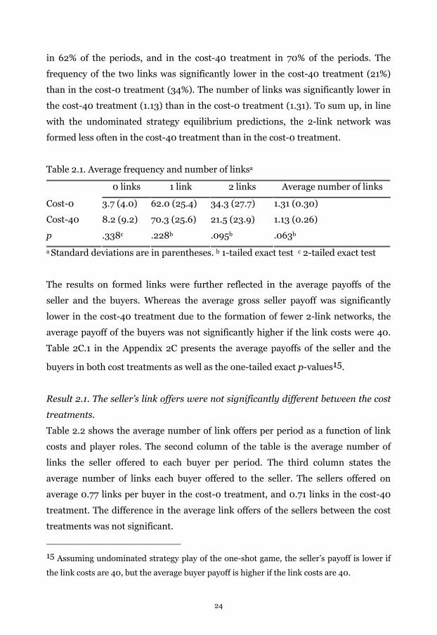
in 62% of the periods, and in the cost-40 treatment in 70% of the periods. The
frequency of the two links was significantly lower in the cost-40 treatment (21%)
than in the cost-0 treatment (34%). The number of links was significantly lower in
the cost-40 treatment (1.13) than in the cost-0 treatment (1.31). To sum up, in line
with the undominated strategy equilibrium predictions, the 2-link network was
formed less often in the cost-40 treatment than in the cost-0 treatment.
Table 2.1. Average frequency and number of linksa
0 links 1 link 2 links Average number of links
Cost-0 3.7 (4.0) 62.0 (25.4) 34.3 (27.7) 1.31 (0.30)
Cost-40 8.2 (9.2) 70.3 (25.6) 21.5 (23.9) 1.13 (0.26)
p .338c .228b .095b .063b
a Standard deviations are in parentheses. b 1-tailed exact test c 2-tailed exact test
The results on formed links were further reflected in the average payoffs of the
seller and the buyers. Whereas the average gross seller payoff was significantly
lower in the cost-40 treatment due to the formation of fewer 2-link networks, the
average payoff of the buyers was not significantly higher if the link costs were 40.
Table 2C.1 in the Appendix 2C presents the average payoffs of the seller and the
buyers in both cost treatments as well as the one-tailed exact p-values15.
Result 2.1. The seller’s link offers were not significantly different between the cost
treatments.
Table 2.2 shows the average number of link offers per period as a function of link
costs and player roles. The second column of the table is the average number of
links the seller offered to each buyer per period. The third column states the
average number of links each buyer offered to the seller. The sellers offered on
average 0.77 links per buyer in the cost-0 treatment, and 0.71 links in the cost-40
treatment. The difference in the average link offers of the sellers between the cost
treatments was not significant.
15 Assuming undominated strategy play of the one-shot game, the seller’s payoff is lower if
the link costs are 40, but the average buyer payoff is higher if the link costs are 40.
24
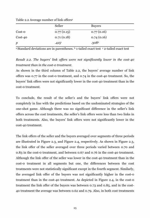
Table 2.2 Average number of link offersa
Seller Buyers
Cost-0 0.77 (0.15) 0.77 (0.16)
Cost-40 0.71 (0.18) 0.74 (0.16)
p .415c .308b
a Standard deviations are in parentheses. b 1-tailed exact test c 2-tailed exact test
Result 2.2. The buyers’ link offers were not significantly lower in the cost-40
treatment than in the cost-0 treatment.
As shown in the third column of Table 2.2, the buyers’ average number of link
offers was 0.77 in the cost-0 treatment, and 0.74 in the cost-40 treatment. So, the
buyers’ link offers were not significantly lower in the cost-40 treatment than in the
cost-0 treatment.
To conclude, the result of the seller’s and the buyers’ link offers were not
completely in line with the predictions based on the undominated strategies of the
one-shot game. Although there was no significant difference in the seller’s link
offers across the cost treatments, the seller’s link offers were less than two links in
both treatments. Also, the buyers’ link offers were not significantly lower in the
cost-40 treatment.
The link offers of the seller and the buyers averaged over segments of three periods
are illustrated in Figure 2.3, and Figure 2.4, respectively. As shown in Figure 2.3,
the link offer of the seller averaged over three periods varied between 0.70 and
0.83 in the cost-0 treatment, and between 0.67 and 0.76 in the cost-40 treatment.
Although the link offer of the seller was lower in the cost-40 treatment than in the
cost-0 treatment in all segments but one, the differences between the cost
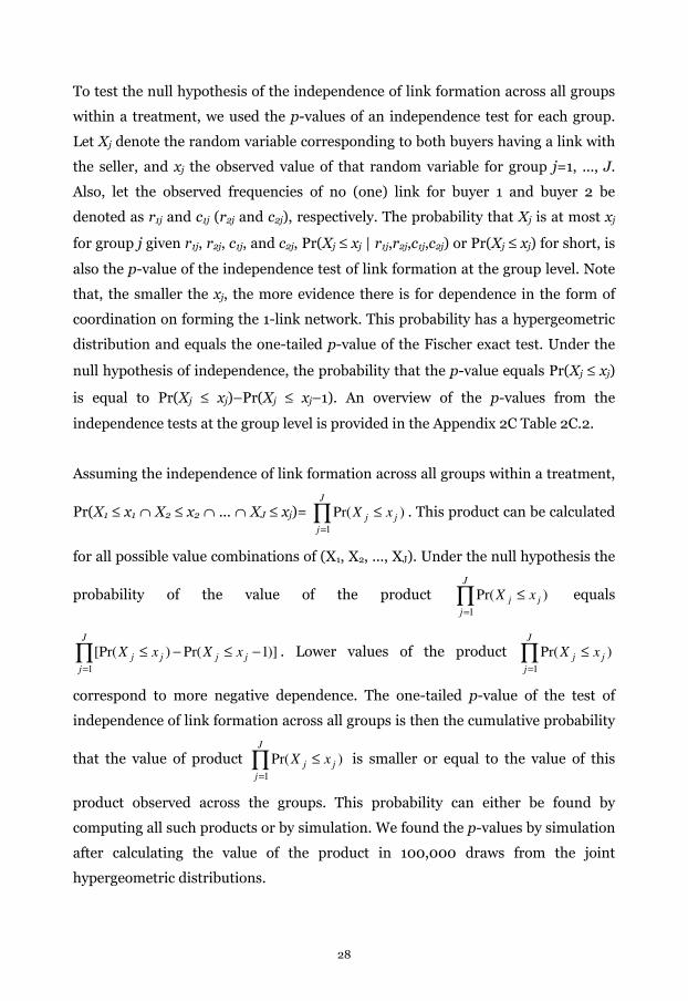
treatments were not statistically significant except in the fourth segment. Similarly,
the averaged link offer of the buyers was not significantly higher in the cost-0
treatment than in the cost-40 treatment. As depicted in Figure 2.4, in the cost-0
treatment the link offer of the buyers was between 0.73 and 0.85, and in the cost-
40 treatment the average was between 0.62 and 0.79. Also, in both cost treatments
25
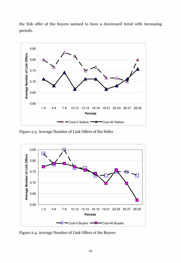
the link offer of the buyers seemed to have a downward trend with increasing
periods.
0,60
0,65
0,70
0,75
0,80
0,85
1-3 4-6 7-9 10-12 13-15 16-18 19-21 22-24 25-27 28-30
Periods
Avera
ge N
um
ber
of
Lin
k O
ffers
Cost-0 Sellers Cost-40 Sellers
Figure 2.3. Average Number of Link Offers of the Seller
0,60
0,65
0,70
0,75
0,80
0,85
1-3 4-6 7-9 10-12 13-15 16-18 19-21 22-24 25-27 28-30
Periods
Avera
ge N
um
ber
of
Lin
k O
ffers
Cost-0 Buyers Cost-40 Buyers
Figure 2.4. Average Number of Link Offers of the Buyers
26

Result 3. Regardless of the cost treatment, the conditional probability that a link
was formed with buyer 1 (2) given that a link was formed with buyer 2 (1) was
significantly smaller than the marginal probability that a link was formed with
buyer 1 (2).
Table 2.3 illustrates the average number of periods buyer 1 and buyer 2 formed a
link with the seller, and the expected number of periods in parentheses. The
frequencies in the cells were calculated by averaging the corresponding cell
frequencies of all groups in a treatment. The expected frequencies of the cells
corresponding to the empty network, given the marginal frequencies of Table 2.3,
were 3.61 and 5.62 for the cost-0 and cost-40 treatment respectively. These
numbers exceeded the observed frequencies by 2.51 (3.61–1.10) and 3.16 (5.62–
2.46) in the cost-0 and cost-40 treatment, respectively, which were in line with our
hypothesis that the conditional probability of having a link is larger if the other
buyer does not have a link. To test the hypothesis statistically we must take into
account that Table 2.3 is the result of combining frequency distributions of groups
that have substantial differences in their marginal frequencies. We first describe
the logic of the test.
Table 2.3 Observed and expected number of linksa,b
Buyer 2
No link Link
Cost-0
No Link 1.10 (3.61) 9.40 (6.90) Buyer 1
Link 9.20 (3.70) 10.30 (12.81)
p:< .001 b
Cost-40
No Link 2.46 (5.61) 9.73 (6.57) Buyer 1
Link 11.36 (8.21) 6.46 (9.61)
p:< .001 b
a Expected number of periods are in parentheses. b 1-tailed exact test
27
To test the null hypothesis of the independence of link formation across all groups
within a treatment, we used the p-values of an independence test for each group.
Let Xj denote the random variable corresponding to both buyers having a link with
the seller, and xj the observed value of that random variable for group j=1, ..., J.
Also, let the observed frequencies of no (one) link for buyer 1 and buyer 2 be
denoted as r1j and c1j (r2j and c2j), respectively. The probability that Xj is at most xj
for group j given r1j, r2j, c1j, and c2j, Pr(Xj ≤ xj | r1j,r2j,c1j,c2j) or Pr(Xj ≤ xj) for short, is
also the p-value of the independence test of link formation at the group level. Note
that, the smaller the xj, the more evidence there is for dependence in the form of
coordination on forming the 1-link network. This probability has a hypergeometric
distribution and equals the one-tailed p-value of the Fischer exact test. Under the
null hypothesis of independence, the probability that the p-value equals Pr(Xj ≤ xj)
is equal to Pr(Xj ≤ xj)–Pr(Xj ≤ xj–1). An overview of the p-values from the
independence tests at the group level is provided in the Appendix 2C Table 2C.2.
Assuming the independence of link formation across all groups within a treatment,
Pr(X1 ≤ x1 ∩ X2 ≤ x2 ∩ ... ∩ XJ ≤ xj)= 1
Pr( )J
j j
j
X x=
≤∏ . This product can be calculated
for all possible value combinations of (X1, X2, ..., XJ). Under the null hypothesis the
probability of the value of the product 1
Pr( )J
j j
j
X x=
≤∏ equals
1
[Pr( ) Pr( 1)]J
j j j j
j
X x X x=
≤ − ≤ −∏ . Lower values of the product 1
Pr( )J
j j
j
X x=
≤∏
correspond to more negative dependence. The one-tailed p-value of the test of
independence of link formation across all groups is then the cumulative probability
that the value of product 1
Pr( )J
j j
j
X x=
≤∏ is smaller or equal to the value of this
product observed across the groups. This probability can either be found by
computing all such products or by simulation. We found the p-values by simulation
after calculating the value of the product in 100,000 draws from the joint
hypergeometric distributions.
28

Applying the test to the link distributions of the groups resulted in a p-value
smaller than .001 for both cost treatments. Thus, in both treatments there was
evidence for coordination behaviour and the proportion of periods in which a 1-link
network was formed was higher than the expected proportion of periods under the
independence assumption.
Result 4. Regardless of the link costs, the probability that buyer 1 (2) offers a link
given that buyer 2 (1) offers a link was significantly smaller than the probability
that buyer 1 (2) offers a link.
Table 2.4 illustrates the average, and expected number of periods buyer 1 and buyer
2 offered a link to the seller. The expected frequencies exceeded the observed
frequencies corresponding to the empty network by 1.35 (1.55–0.20) and 0.91
(2.00–1.09) for the cost-0 and cost-40 treatment respectively. This was in line with
our hypothesis that the conditional probability of a buyer offering a link is larger
conditional on the other buyer not offering a link. Applying the same test as in
Result 3, we rejected the null hypothesis of independence with p-values smaller
than .001 for both cost treatments. Thus, in both cost treatments there was
evidence for buyer coordination.
Table 2.4 Observed and expected number of periods of buyer link offersa
Buyer 2
No link Offer Link Offer
Cost-0
No Link Offer 0.20 (1.55) 5.70 (4.35) Buyer 1
Link Offer 7.70 (6.35) 16.40 (17.75)
p: <.001 b
Cost-40
No Link Offer 1.09 (2.00) 5.64 (4.73) Buyer 1
Link Offer 7.82 (6.91) 15.46 (16.36)
p: <.001 b
a Expected number of periods are in parentheses. b 1-tailed exact test.
29
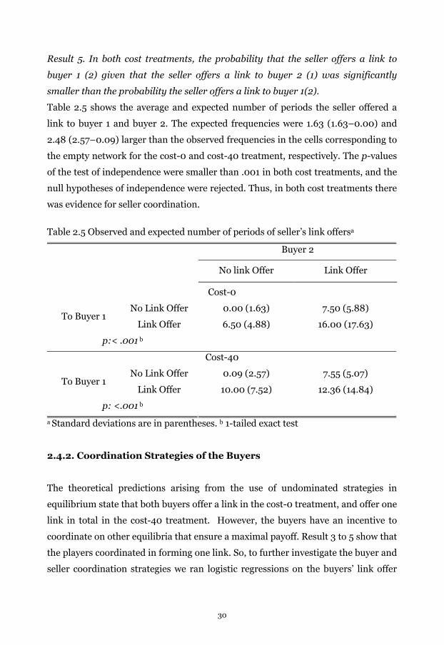
Result 5. In both cost treatments, the probability that the seller offers a link to
buyer 1 (2) given that the seller offers a link to buyer 2 (1) was significantly
smaller than the probability the seller offers a link to buyer 1(2).
Table 2.5 shows the average and expected number of periods the seller offered a
link to buyer 1 and buyer 2. The expected frequencies were 1.63 (1.63–0.00) and
2.48 (2.57–0.09) larger than the observed frequencies in the cells corresponding to
the empty network for the cost-0 and cost-40 treatment, respectively. The p-values
of the test of independence were smaller than .001 in both cost treatments, and the
null hypotheses of independence were rejected. Thus, in both cost treatments there
was evidence for seller coordination.
Table 2.5 Observed and expected number of periods of seller’s link offersa
Buyer 2
No link Offer Link Offer
Cost-0
No Link Offer 0.00 (1.63) 7.50 (5.88) To Buyer 1
Link Offer 6.50 (4.88) 16.00 (17.63)
p:< .001 b
Cost-40
No Link Offer 0.09 (2.57) 7.55 (5.07) To Buyer 1
Link Offer 10.00 (7.52) 12.36 (14.84)
p: <.001 b
a Standard deviations are in parentheses. b 1-tailed exact test
2.4.2. Coordination Strategies of the Buyers
The theoretical predictions arising from the use of undominated strategies in
equilibrium state that both buyers offer a link in the cost-0 treatment, and offer one
link in total in the cost-40 treatment. However, the buyers have an incentive to
coordinate on other equilibria that ensure a maximal payoff. Result 3 to 5 show that
the players coordinated in forming one link. So, to further investigate the buyer and
seller coordination strategies we ran logistic regressions on the buyers’ link offer
30

decisions given the link offer decisions of the previous period, and the results are
displayed in Table 2.6.
The model captures the effect of the following variables in the previous period on
the probability of a buyer offering a link to the seller: a 1-link network in which the
buyer forms a link (own link), a 1-link network in which the other buyer is linked
(other link), and a two link network (two links)16. Thus, we controlled for the effect
of the variables which are predicted to have an effect according to the coordination
equilibria. We also controlled for period, and all the interaction effects with period.
Period was grouped into 6 segments and centered, i.e for the periods 1-5, 6-
10,...,25-30 the values of the variable period were –2.5, –1.5,..., 2.5 respectively. We
ran separate logistic regressions for the two cost treatments because the results of
the logistic regression containing both treatments showed strong effects of the
treatment with the variables own link times period, other link times period, and
two links times period. Such strong effects suggested the use of different strategies
in the two treatments. The logistic regression results including the treatment and
the interactions with the treatment are shown in the Appendix 2C Table 2C.3. Table
2.6 shows the coefficients, and the corresponding p-values of the variables from the
regression on the cost-0 (cost-40) treatment in the second and third (fourth and
fifth) columns. The p-values are one-tailed for the variables in which an effect is
predicted by the buyer or seller equilibrium, and two-tailed otherwise. The
standard errors are stated in parentheses. The last two columns of the table show
the predictions of the buyer and the seller coordination equilibrium. A positive
(negative) sign indicates that the equilibrium predicts a positive (negative) effect of
that variable on the buyer’s probability of offering a link. For all the other variables,
the buyer or the seller coordination equilibria have no prediction on their effect.
16 So, the network effects were captured with three dummies, and the constant in the
regression referred to the empty network.
31
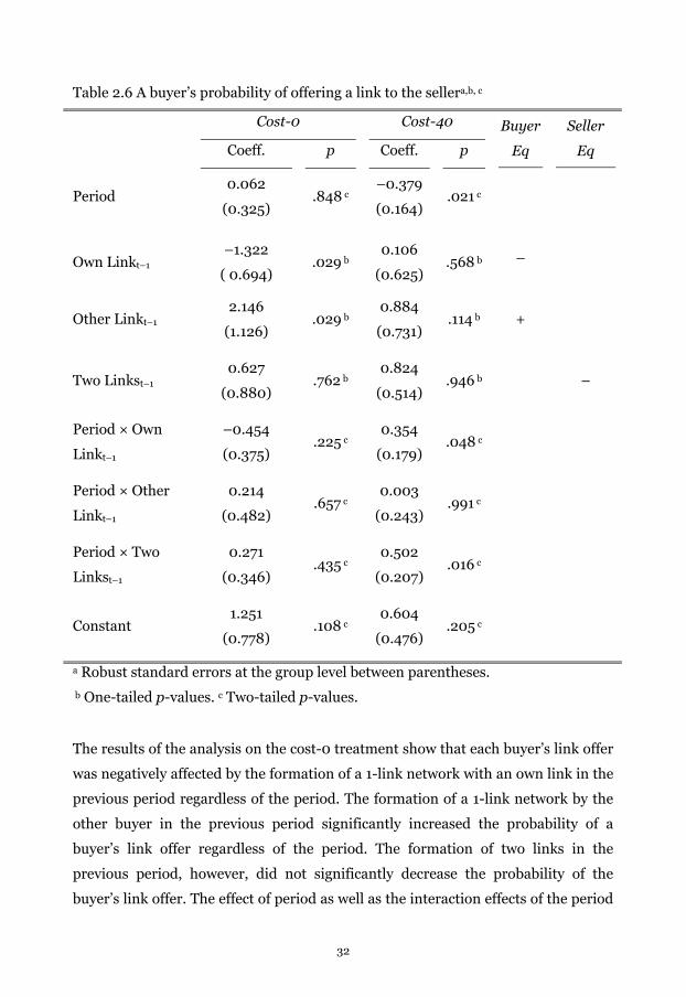
Table 2.6 A buyer’s probability of offering a link to the sellera,b, c
Cost-0 Cost-40
Coeff. p Coeff. p
Buyer
Eq
Seller
Eq
Period 0.062
(0.325) .848 c
–0.379
(0.164) .021 c
Own Linkt–1 –1.322
( 0.694) .029 b
0.106
(0.625) .568 b –
Other Linkt–1 2.146
(1.126) .029 b
0.884
(0.731) .114 b +
Two Linkst–1
0.627
(0.880) .762 b
0.824
(0.514) .946 b –
Period × Own
Linkt–1
–0.454
(0.375) .225 c
0.354
(0.179) .048 c
Period × Other
Linkt–1
0.214
(0.482) .657 c
0.003
(0.243) .991 c
Period × Two
Linkst–1
0.271
(0.346) .435 c
0.502
(0.207) .016 c
Constant 1.251
(0.778) .108 c
0.604
(0.476) .205 c
a Robust standard errors at the group level between parentheses.
b One-tailed p-values. c Two-tailed p-values.
The results of the analysis on the cost-0 treatment show that each buyer’s link offer
was negatively affected by the formation of a 1-link network with an own link in the
previous period regardless of the period. The formation of a 1-link network by the
other buyer in the previous period significantly increased the probability of a
buyer’s link offer regardless of the period. The formation of two links in the
previous period, however, did not significantly decrease the probability of the
buyer’s link offer. The effect of period as well as the interaction effects of the period
32
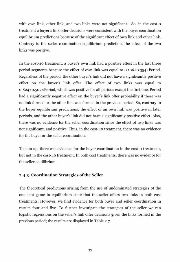
with own link, other link, and two links were not significant. So, in the cost-0
treatment a buyer’s link offer decisions were consistent with the buyer coordination
equilibrium predictions because of the significant effect of own link and other link.
Contrary to the seller coordination equilibrium prediction, the effect of the two
links was positive.
In the cost-40 treatment, a buyer’s own link had a positive effect in the last three
period segments because the effect of own link was equal to 0.106+0.354×Period.
Regardless of the period, the other buyer’s link did not have a significantly positive
effect on the buyer’s link offer. The effect of two links was equal to
0.824+0.502×Period, which was positive for all periods except the first one. Period
had a significantly negative effect on the buyer’s link offer probability if there was
no link formed or the other link was formed in the previous period. So, contrary to
the buyer equilibrium predictions, the effect of an own link was positive in later
periods, and the other buyer’s link did not have a significantly positive effect. Also,
there was no evidence for the seller coordination since the effect of two links was
not significant, and positive. Thus, in the cost-40 treatment, there was no evidence
for the buyer or the seller coordination.
To sum up, there was evidence for the buyer coordination in the cost-0 treatment,
but not in the cost-40 treatment. In both cost treatments, there was no evidence for
the seller equilibrium.
2.4.3. Coordination Strategies of the Seller
The theoretical predictions arising from the use of undominated strategies of the
one-shot game in equilibrium state that the seller offers two links in both cost
treatments. However, we find evidence for both buyer and seller coordination in
results four and five. To further investigate the strategies of the seller we ran
logistic regressions on the seller’s link offer decisions given the links formed in the
previous period; the results are displayed in Table 2.7.
33
Table 2.7 Seller’s probability of offering a link to a buyera, b, c
Cost-0 Cost-40
Coefficient p Coefficient p Seller Eq
Period –0.040
(0.209) .848 c
0.187
(0.126) .139 c
Own Linkt–1 –0.796
(0.671) .118 b
–0.518
(0.725) .238 b –
Other Linkt–1 1.980
(0.674) .002 b
–0.967
(0.626) .938 b +
Two Linkst–1
1.128
(0.812) .165 c
0.448
(0.439) .307 c
Period × Own Linkt–1 –0.093
(0.250) .712 c
–0.151
(0.110) .171 c
Period × Other Linkt–1 0.037
(0.232) .872 c
–0.172
(0.145) .237 c
Period × Two Linkst–1 0.125
(0.258) .627 c
–0.061
(0.249) .808 c
Constant 0.746
(0.506) .140 c
1.344
(0.256) <.001 c
a Robust standard errors at the group level between parentheses.
b One-tailed p-values. c Two-tailed p-values.
Similar to the analysis with the buyers’ link offers, we ran separate analyses for the
two cost treatments. In the logistic regressions the seller’s probability of offering a
link to a particular buyer was the dependent variable with the same control
variables mentioned in subsection 2.4.2. So, the variables that account for the
formation of 1-link or 2-link networks, and that the equilibria have predictions on
were included in the regression and period was grouped into 6 segments. The
coefficients, and the corresponding p-values of the variables from the regression on
the cost-0 (40) treatment are shown in the second and third (fourth and fifth)
34
columns of Table 2.7. The standard errors are stated in parentheses. The last
column of the table shows the predictions of the seller coordination equilibrium.
The buyer equilibrium does not have predictions for the effect of any of the
variables. A positive (negative) sign indicates that the seller equilibrium predicts a
positive (negative) effect of that variable on the seller’s probability of offering a
link. No sign indicates that the seller equilibrium does not prescribe a prediction
for that variable. The p-values are one-tailed for the variables in which an effect is
predicted by seller equilibrium, and two-tailed otherwise. Also, the logistic
regression results including the treatment and the interactions with the treatment
are included in the Appendix 2C Table 2C.4. This analysis showed strong effects of
the treatment with the variable other link suggesting the use of different strategies
in the two treatments.
In the cost-0 treatment, the results of the regression show that the formation of a 1-
link network with a particular buyer in the previous round did not significantly
decrease the probability of the seller’s link offer to that buyer. In line with the seller
equilibrium the seller’s probability of offering a link to a buyer significantly
increased with the formation of a 1-link network with the other buyer. In sum,
there was some evidence in line with the seller coordination in the cost-0
treatment.
The cost-40 treatment results demonstrate that the probability of the seller’s link
offer to a particular buyer did not significantly decrease (increase) after the
formation of an own link (other link) in the previous period. Also, the variables two
links, period, and the interaction effects with the period were not significant. So
there was no support for the seller equilibrium in the cost-40 treatment.
To sum up, there was some evidence in the cost-0 treatment for the seller
equilibrium, but not in the cost-40 treatment. Note that, the buyer equilibrium had
no predictions on the effect of any of the variables.
35
2.4.4. Link Formation Results at the Group Level
Results 3 to 5 provide evidence for the coordination of link formation, link offers of
the buyers and link offers of the seller in both cost treatments. The logistic
regression results for the cost-0 treatment are parallel to these results such that
buyer coordination predictions were supported by the strategies of the buyers, and
there was some evidence in support of the seller coordination. However, in the
cost-40 treatment, the logistic regression results show no evidence for the buyer
coordination or the seller coordination. So, there was evidence for coordination in
the cost-40 treatment based on the independence tests, but no such evidence was
found from the logistic regressions. The mixed results might arise from different
strategies that different groups employed within the cost-40 treatment. It is also
possible that players used strategies other than buyer or seller equilibrium which
led to the formation of a 1-link network in every period. As an example, the seller
might form a link with the same buyer for 15 consecutive periods, and form a link
with the other buyer in the remaining 15 periods. Logistic regression results do not
pick up such coordination behaviour. Therefore, we investigated link offer
decisions at the group level using the exact test that was explained in Result 3. Note
that this exact test successfully picks up different types of coordination behaviour
such as the one in the previous example.
To categorize the groups according to their strategies, we mainly relied on the test
results of the independence of the buyers’ link offers (as in Result 4) and the
independence of the seller’s link offers (as in Result 5). To be precise, if the test
results of the independence test for the buyers’ (seller’s) link offers was significant,
then that group was classified as playing the buyer (seller) coordination if it also
satisfied the following conditions. For the buyer coordination, the difference
between the following two numbers was not higher than 10: the number of periods
buyer 1 offered a link to the seller and buyer 2 did not offer a link, and the number
of periods buyer 2 offered a link to the seller and buyer 1 did not. Similarly, for the
seller coordination, the difference between the following two numbers was not
higher than 10: the number of periods the seller offered a link only to buyer 2, and
the number of periods the seller offered a link only to buyer 1. The rationale for the
36
additional conditions was to prevent wrongly specifying the groups in which there
was coordination on forming one link with the same buyer in most of the cases.
This situation is referred to as ‘one buyer only’. In such a situation the link offers of
the buyers might significantly depend on each other (likewise for the seller), hence
leading to a significant p-value in the test for independence. However, since in this
paper coordination is defined as forming one link that maximizes the payoff of each
buyer in a repeated setting while maintaining equality, the aforementioned
situations were not classified as coordination17.
A group was said to play similar to buyer (seller) coordination equilibrium if there
was no significant p-value for the independence of the buyers’ (seller’s) link offers,
but a 1-link network was formed in majority of the periods, and the above condition
for the buyers (seller) held. An overview of the independence test results for each
group is included in the Appendix 2C Table 2C.2. In this table, the groups are
arranged according to the order of their mention in this section. All reported p-
values in this section are one-tailed.
In the cost-0 treatment 7 out of 10 groups engaged in coordination. Among these
seven groups there was one group with both buyer and seller coordination, three
groups played the buyer coordination, and the other three groups played the seller
coordination. The remaining three groups of the cost-0 treatment played similar to
the undominated strategy of the one-shot game, i.e., these groups formed two links
17 Limiting the maximum difference between link offers to 10 periods or using a similar rule
does not affect the categorization of the groups dramatically. For the differences between
link offers between 10 and 25, the categorization would be the same as in this paper.
Dropping these conditions altogether would lead to a change in the categorization of only
one group. Making the conditions stricter would, however, lead some groups to be dropped
from the coordination category depending on how small the chosen number is. Choosing
another rule such as limiting the difference between the formed links of buyer 1 and buyer 2
to 10 would lead to the same categorization as in this paper. Nonetheless, there is a need to
define a coordination index or heuristic that would lead to consistent and meaningful
categorizations. The author of this paper is not aware of any such index that is applicable to
this analysis.
37

in most periods. The categories of strategies in both cost treatments along with the
number of groups playing those strategies are summarized in Table 2.8.
Table 2.8 Number of groups playing different strategies
Cost-0 Cost-40
Buyer & Seller Coordination 1 2
Buyer Coordination 3 1
Seller Coordination 3 1
Similar to Coordination - 2
One Buyer only - 3
(Un)dominated Strategy 3 2
Total 10 11
In the first group of the cost-0 treatment, both buyer and seller coordination
strategy play was observed; the buyers offered in total one link in 21 periods and
the seller offered in total one link in 24 periods. 1-link networks were formed with
each buyer for 13 periods.
In groups 2 to 4, there was similar play to the buyer coordination equilibrium; the
buyers offered in total one link in 25, 23, and 24 periods, and the seller offered two
links in 13, 19, and 16 periods. In these groups, a 1-link network was formed in 25,
22, and 24 periods with the buyers having roughly the same number of 1-link
networks.
Third, in the three groups with similar play to the seller coordination equilibrium
(groups 5 to 7), the buyers offered two links in 15, 30, and 24 periods, the seller
offered one link in 27, 18, and 19 periods, and a 1-link network was formed in 26,
18, and 19 periods, respectively. In these three groups there was one buyer who
always offered a link. Note that in none of these groups there was evidence for
punishment after the formation of two links.
Finally, the repeated play of the undominated strategy equilibrium of the one-shot
game was observed in three groups. In these three groups, the sellers offered two
38
links in 30, 30, and 20 periods, both buyers offered a link in 22, 25, and 22 periods,
and as a result, two links were formed in 22, 25, and 16 periods respectively. Also,
in all the three groups there was evidence of an attempted buyer coordination that
failed such that one buyer alternated between offering and not offering a link at the
beginning of the game, but the other buyer did not reciprocate. Notice that such
repeated play is also a SPE of the game.
In the cost-40 treatment, 4 out of 11 groups played the coordination equilibria, and
two other groups played similar to the coordination equilibria. Among the four
coordinating groups, in two groups both buyer and seller coordination were
observed, in one group there was buyer coordination, and one group played the
seller equilibrium. In the two groups that played similar to the coordination
equilibria, one group’s play was similar to the buyer equilibrium, and the other
group’s play was similar to the seller equilibrium.
In the remaining five groups of the cost-40 treatment, two types of play other than
coordination were observed. In three groups a 1-link network was observed almost
exclusively with the same buyer, and in two groups there was “dominated strategy”
play, leading to the formation of 2-link networks in the majority of the periods.
Notice that such a strategy was dominated for the buyers in the cost-40 treatment.
In the groups 1 and 2 in which both the buyers and the seller coordinated, the
buyers offered one link in total in 22, and 26 periods, and the sellers offered one
link in 28, and 25 periods. In these two groups a 1-link network was formed with
alternating buyers in 30, and 28 periods respectively. In group 3 there was buyer
coordination; the buyers offered one link in total in 21 periods, the seller offered
two links in 20 periods, and a 1-link network was formed in 18 periods. Group 4
could be considered as playing the seller coordination. In this group the buyers
offered two links in 21 periods, the seller offered one link in 17 periods, and a 1-link
network was formed in 16 periods. In this group the seller also formed two links in
some periods without being punished afterwards.
39

Groups 5 and 6 could be considered as playing similar to the coordination
equilibria. In group 5, the buyers offered one link in total in 17 periods, and the
seller offered two links in 30 periods. A 1-link network was formed in 17 periods. In
this group the buyers seemed to learn to alternate their link offers over time albeit
not totally successfully. Group 6 could be considered as playing the seller
coordination. The buyers in this group offered two links in 19 periods and the seller
offered one link in 16 periods. In this group, 1-link networks were formed in 18
periods. However, there was not enough power to reject the independence
hypothesis for the seller’s link offer decisions.
Different from the cost-0 treatment, in the cost-40 treatment there were groups in
which in almost all periods a 1-link network was formed with the same buyer. In
groups 7 to 9, the buyers offered two links in 6, 24, and 28 periods, and the sellers
of these groups offered a link to the same buyer in almost all periods (27, 29 and 27
periods respectively). In the first group both buyers offered two links in six out of
the first nine periods, and after the ninth period one buyer did not offer a link
whereas in the latter two groups buyers offered two links in most periods. Although
in the last group the independence test showed a significant effect for the seller’s
link offers (p-value: .007), the coordination condition was not satisfied for the
seller, i.e., the seller offered one link to buyer 1 in 27 periods, one link to buyer 2 in
2 periods and the difference between the two was more than 10. Notice that the
strategies of the players in these three groups constitute a SPE of the repeated
game18. Also, in all groups the seller offered two links in the last period implying
that the sellers played equilibrium strategies until the last period in which a
deviation could not be punished.
The last two groups’ play was similar to the undominated strategy play of the one-
shot game in the cost-0 treatment. In these two groups the seller offered two links
in 22, and 26 periods, and the buyers offered two links in 22, and 24 periods
18 It can be shown that it is a SPE of the repeated game that both buyers always offer a link,
and the seller always offers a link to the same buyer. If the seller deviates and offers two
links, then both buyers punish the seller for at least one period by not offering a link.
40
respectively. As a result two links were formed in 15, and 22 periods, respectively
which led to substantial losses for both buyers. Although given that the seller
offered two links, and one buyer always offered a link, the other buyer was better
off by not offering a link, both buyers did not deviate from offering a link in the
majority of the periods. As in the groups that played the undominated strategy in
the cost-0 treatment, in these two groups one buyer tried to coordinate at the
beginning of the game, but the other buyer did not reciprocate and kept on offering
a link to the seller in every period. Note that such buyer behaviour was not only
contrary to the repeated SPE predictions, but also to the predictions of the
inequality aversion models such as Fehr and Schmidt (1999), Bolton and Ockenfels
(2000), and a preference for efficiency19.
To sum up, in the cost-0 treatment, seven out of 10 groups engaged in some sort of
coordination behaviour. In the other three groups, the undominated strategy play
was prevalent. In the cost-40 treatment, four out of 11 groups played coordination
equilibria. In two other groups the strategies were similar to coordination play. In
three groups players coordinated on forming one link with the same buyer only.
Finally, there were two groups who played contrary to the theoretical predictions.
So, in both cost treatments the majority of the groups played similar to the
coordination predictions using the buyer or the seller coordination strategies or
both. Remarkably, the number of coordinating groups did not increase with link
costs.
2.5. Discussion and Conclusion
In this paper we examined the impact of the link costs on network formation.
Particularly, we addressed the questions of whether the players coordinated on
forming the non-competitive networks, who facilitated the coordination, and
whether link costs affected the coordination behaviour.
19 Assuming that the seller always offers two links, and one of the buyers always offers one
link as was the case in these three groups, then according to these models the other buyer is
better off by not offering a link regardless of the parameter values.
41
To investigate these questions we implemented a finitely repeated game between
one seller and two potential buyers. The seller decided whether to form one or two
links with the buyers and the buyers simultaneously decided whether to form a link
with the seller. If a competitive network was formed in which the seller was linked
to both buyers, then the seller earned the entire surplus. In a one link network the
surplus was shared between the seller and the linked buyer. We studied the
repeated game subgame perfect equilibria with and without link costs. If the
players used undominated strategies of the one-shot game, the presence of link
costs was predicted to reduce the occurrence of competitive networks. We have
shown that, regardless of the link costs, the formation of one link with alternating
buyers in which the buyers anti-coordinate their actions and take-turns was a
repeated game subgame perfect equilibrium. Moreover, coordination on forming
one link that is facilitated by the seller could also be supported as a subgame
perfect equilibrium. We thus investigated whether coordinated existed, and if so
who facilitated the coordination.
We found that with link costs, a competitive network in which the seller was linked
to both buyers was less likely to be formed. Although the average number of links
was significantly lower with link costs, the seller’s or the buyers’ link offers were not
significantly different across the cost treatments. Thus, both the seller and the
buyers coordinated their link offers if the link costs were positive so as to form the
competitive network less often. Moreover, sellers did not employ the weakly
dominating strategy (of the one-shot game) of offering two links regardless of the
link costs.
We found strong evidence for coordination on forming one link in both cost
treatments. The test results on both treatments showed highly significant
dependence of i) the link formation of one buyer on the link formation of the other
buyer, ii) a buyer’s link offer on the link offer of the other buyer, and iii) the seller’s
link offer to one buyer on the seller’s link offer decision on the other buyer. The
logistic regressions that controlled for the effect of the links formed in the previous
period on the buyer’s and the seller’s link offer probability provided some support
42

for both the buyer and the seller coordination strategies if the links were costless.
However, the logistic regression results were contrary to the buyer or seller
coordination strategies if the link costs were positive. Such mixed results in the
positive link cost treatment resulted from different strategies that groups employed
if the links were costly.
The analysis at the group level showed that if the links were costless, seven out of
10 groups engaged in some sort of coordination behaviour. If the link costs were
positive, four out of 11 groups played coordination equilibria, and two other groups
played similar to coordination equilibria. Among the coordinating groups, some
engaged in the buyer coordination, some in the seller coordination, and some in
both. So, in both cost treatments the majority of the groups played similar to the
coordination equilibria. Notably, and contrary to what one might expect, the
number of coordinating groups did not increase with the link costs.
Our group level results pointed to two types of play that deserves special attention.
First, if the links were costly, there were three groups in which one link was formed
with the same buyer in almost all periods. In these three groups, the seller
facilitated the formation of one link networks but did not “coordinate”. So, clearly,
the sellers of these groups did not care about the payoff inequality across the
buyers. The second type of play that deserves special attention is the dominated
strategy play: If the links were costly in two groups two links were formed in most
periods causing the buyers to earn negative payoffs. Such buyer behaviour cannot
be explained by the profit maximizing rational agents even if inequality aversion or
preference for efficiency is taken into consideration. Thus, these buyers might have
social preferences that cannot be captured with the inequality aversion models .
Our findings on anti-coordinating on a mutually beneficial outcome by alternating,
i.e., buyer coordination, was in line with the findings of the repeated chicken and
battle of the sexes games investigated by Rapoport, Guyer and Gordon (1976) and
Arifovic et al. (2006) respectively. Different from these studies, however, in our
game anti-coordination involved more than two players. Also, a third party who
had a weakly dominating strategy in the one-shot game could also coordinate on
43
the mutually beneficial outcome of the other two players. We found evidence for
both coordination and anti-coordination behaviour in a 3-player game with a rich
setting. For future research, it would be interesting to study (anti-) coordination
behaviour in network formation games of more than three players. Also, running
our experiments with random matching would provide insights on whether the
seller behaviour depended on the repetition of the game or was driven by a
preference for distributional equality.
In sum, the present paper shows that in markets that require connections to be
established between transacting agents, coordinating on the non-competitive
outcome which maximizes the long-run payoffs of the long side of the market is
common. Moreover, coordination does not only arise from the behaviour of the
long side of the market, but from the short side as well.
44

Appendix 2A. List of Networks
Figure 2A.1. Networks according to the number of links
No-Link Networks:
seller seller seller
buyer 1 buyer 2 buyer 1 buyer 2 buyer 1 buyer 2
seller seller seller
buyer 1 buyer 2 buyer 1 buyer 2 buyer 1 buyer 2
seller seller seller
buyer 1 buyer 2 buyer 1 buyer 2 buyer 1 buyer 2
45
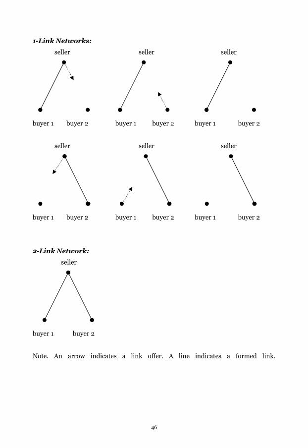
1-Link Networks:
seller seller seller
buyer 1 buyer 2 buyer 1 buyer 2 buyer 1 buyer 2
seller seller seller
buyer 1 buyer 2 buyer 1 buyer 2 buyer 1 buyer 2
2-Link Network:
seller
buyer 1 buyer 2
Note. An arrow indicates a link offer. A line indicates a formed link.
46
Appendix 2B. Experimental Instructions for the Cost-40 Treatment
Introduction
Welcome to this experiment on decision making. We will first go through the
instructions together. Then there will be a practice period. After the practice period
the experiment will start. Talking is strictly forbidden during the experiment. If you
have a question, please raise your hand and I will come to your table to answer your
question.
The experiment will last about 1 hour. If you follow the instructions carefully you
can earn a considerable amount of money. During the experiment your earnings
will be denoted in points. After the experiment your earnings will be converted into
money at a rate of 1 point is 0.35 Eurocents. In addition, you will receive a show-up
fee of 5 Euros. Your earnings will be paid to you, privately and in cash, immediately
after the experiment.
Instructions for the experiment
In this experiment, you are in a group of 3 persons. Each person has her or his own
number; 1, 2, or 3. Your number is randomly determined at the beginning of the
practice period and it stays the same throughout the whole experiment. Also, the
composition of your group remains the same throughout the experiment. You will
not know who is in your group. You and your group members are referred to as
player 1, player 2 and player 3.
Your group faces the same task for 30 periods. In each period, you make a decision
about whether to offer links to other players in your group or not.
A link is formed between two players if both of them offer a link to each other.
Player 1 can have two links; player 2 and 3 can have only one. Hence player 2 and
player 3 each have to decide whether they want to offer a link to player 1. Player 1
has to decide whether to offer a link to player 2 and whether to offer a link to player
3. Offering a link is not costly. However, each player has to pay 40 points for each
link that he has formed.
47

Depending on the links that form, a maximum of 240 points is shared among the
players that form a link with each other. There are 4 different types of situations
that can arise from the players’ decisions to offer links to other players. The
earnings of the players differ across these four situations.
SITUATION A:
1
2 3
In Situation A there are no links. This occurs when player 1 and player 3 do not
both offer a link to each other, and player 1 and player 2 do not both offer a link to
each other. No points are shared among the three players. And since no links have
formed, no player pays any linking costs. Hence players 1, 2, and 3 earn 0 – 0 = 0
points.
SITUATION B:
1
2 3
In Situation B there is only one link, namely between player 1 and player 3. This
occurs when both player 1 and player 3 offer a link to each other, while player 1 and
player 2 do not both offer a link to each other.
The 240 points are shared among player 1 and player 3 in the following way; Player
1 gets 160 points and player 3 gets 80 points. Both player 1 and player 3 pay 40
48
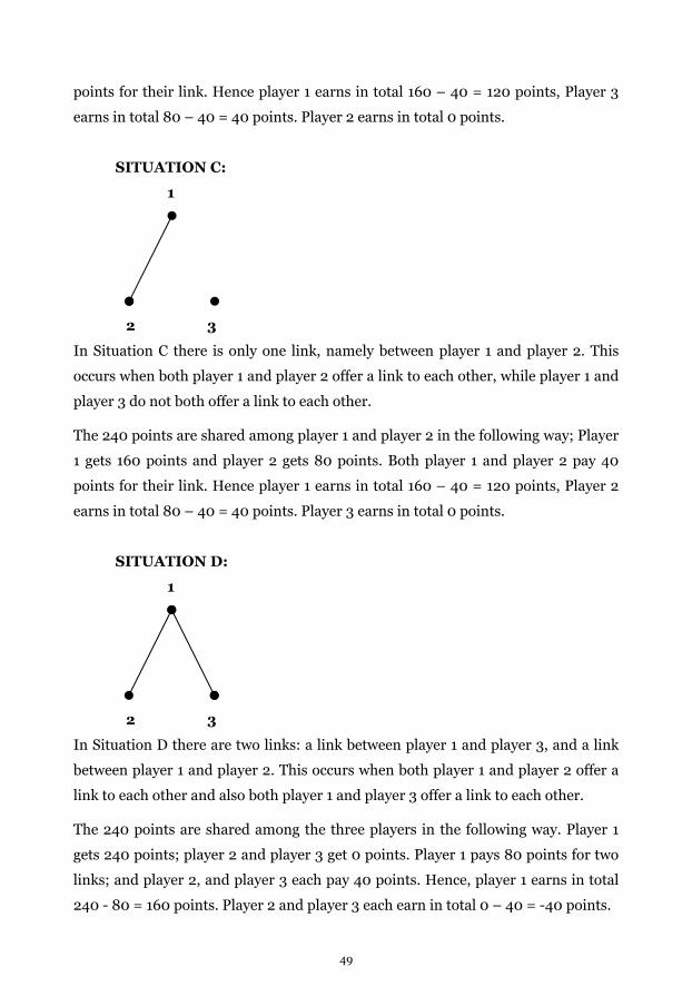
points for their link. Hence player 1 earns in total 160 – 40 = 120 points, Player 3
earns in total 80 – 40 = 40 points. Player 2 earns in total 0 points.
SITUATION C:
1
2 3
In Situation C there is only one link, namely between player 1 and player 2. This
occurs when both player 1 and player 2 offer a link to each other, while player 1 and
player 3 do not both offer a link to each other.
The 240 points are shared among player 1 and player 2 in the following way; Player
1 gets 160 points and player 2 gets 80 points. Both player 1 and player 2 pay 40
points for their link. Hence player 1 earns in total 160 – 40 = 120 points, Player 2
earns in total 80 – 40 = 40 points. Player 3 earns in total 0 points.
SITUATION D:
1
2 3
In Situation D there are two links: a link between player 1 and player 3, and a link
between player 1 and player 2. This occurs when both player 1 and player 2 offer a
link to each other and also both player 1 and player 3 offer a link to each other.
The 240 points are shared among the three players in the following way. Player 1
gets 240 points; player 2 and player 3 get 0 points. Player 1 pays 80 points for two
links; and player 2, and player 3 each pay 40 points. Hence, player 1 earns in total
240 - 80 = 160 points. Player 2 and player 3 each earn in total 0 – 40 = -40 points.
49

The figure above illustrates how the results of the first part of the period are
displayed to you on the computer screen. A black line indicates that both players
offered a link to each other. A red arrow indicates that one player offered a link but
the other player did not offer a link to that one player. So, in this example the black
line indicates that player 1 (which is “You” in this case) and player 2 offered a link
to each other and as a result a link is formed between them.
In this situation (which corresponds to situation C above), player 1 gets 160 points
from one link and pays 40 points for the link. So, player 1 earns in total 120 points.
Player 2 gets 80 points from the link and pays 40 points for the link. So, player 2
earns in total 40 points. The red arrow indicates that player 3 offered a link to
player 1 while player 1 did not offer a link to player 3. Therefore no link is formed
between player 1 and player 3. Player 3 does not pay for offering a link. Player 3
earns in total 0 points. Notice that for each player the total earnings for the period
are indicated in parentheses.
To summarize:
You will be in a group of 3 persons. Each person will have her or his own number; 1,
2, or 3. Your number will be randomly determined at the beginning of the practice
period and it will stay the same throughout the experiment. Also, the composition
50

of your group will remain the same throughout the experiment. You will not know
who is in your group.
There will be 30 periods in the experiment. In every period you will decide with
whom to link. The important points of the experiment are the following:
• A link is formed between two players if both of them offer a link to each
other.
• Player 2 and player 3 cannot form a link with each other.
• Offering a link is not costly but if a link is formed, then players who
have the link each pay 40 points for the link.
• If there is at least one link, the three players share 240 points among
them.
• The earnings of players in each period are equal to the earnings from a
link or links minus the cost of having a link/s.
• In each period you will be informed about all the decisions made by
your group members. At the end of each period, you will be informed
about your and other players’ earnings.
• Your total earnings will be the sum of all points you earn over all
periods. For each point you earn in the experiment, you will get 0.35
Eurocents.
Appendix 2C. Tables
Table 2C.1 The average gross payoff of the seller and the buyersa, b Seller Buyers Cost-0 181.60
(26.71) 24.80 (10.14)
Cost-40 164.12 (24.27)
28.12 (10.23)
p .041 .228 a Standard deviations are in parentheses. b One-tailed exact p-values.
51
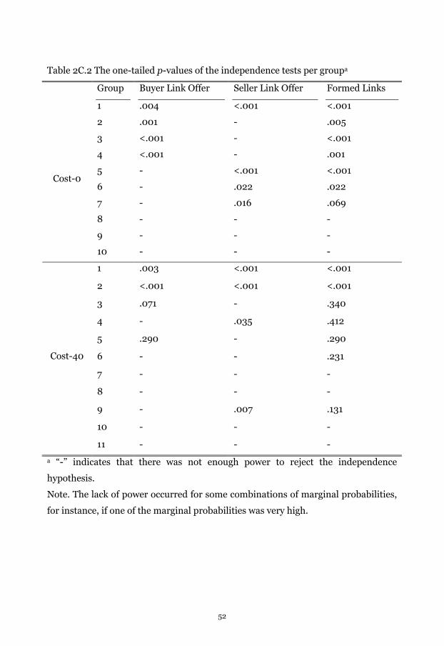
Table 2C.2 The one-tailed p-values of the independence tests per groupa
Group Buyer Link Offer Seller Link Offer Formed Links
1 .004 <.001 <.001
2 .001 - .005
3 <.001 - <.001
4 <.001 - .001
5 - <.001 <.001
6 - .022 .022
7 - .016 .069
8 - - -
9 - - -
Cost-0
10 - - -
1 .003 <.001 <.001
2 <.001 <.001 <.001
3 .071 - .340
4 - .035 .412
5 .290 - .290
6 - - .231
7 - - -
8 - - -
9 - .007 .131
10 - - -
Cost-40
11 - - -
a “-” indicates that there was not enough power to reject the independence
hypothesis.
Note. The lack of power occurred for some combinations of marginal probabilities,
for instance, if one of the marginal probabilities was very high.
52
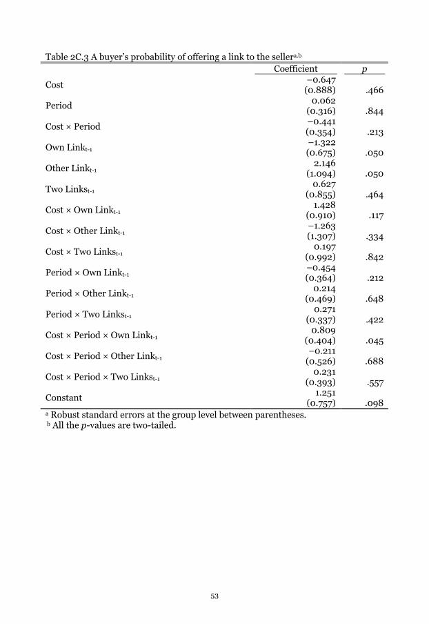
Table 2C.3 A buyer’s probability of offering a link to the sellera.b Coefficient p
Cost –0.647
(0.888) .466
Period 0.062
(0.316) .844
Cost × Period –0.441 (0.354) .213
Own Linkt-1 –1.322 (0.675) .050
Other Linkt-1 2.146
(1.094) .050
Two Linkst-1 0.627
(0.855) .464
Cost × Own Linkt-1 1.428
(0.910) .117
Cost × Other Linkt-1 –1.263 (1.307) .334
Cost × Two Linkst-1 0.197
(0.992) .842
Period × Own Linkt-1 –0.454 (0.364) .212
Period × Other Linkt-1 0.214
(0.469) .648
Period × Two Linkst-1 0.271
(0.337) .422
Cost × Period × Own Linkt-1 0.809
(0.404) .045
Cost × Period × Other Linkt-1 –0.211
(0.526) .688
Cost × Period × Two Linkst-1 0.231
(0.393) .557
Constant 1.251
(0.757) .098 a Robust standard errors at the group level between parentheses. b All the p-values are two-tailed.
53

Table 2C.4 The seller’s probability of offering a link to a buyera.b Coefficient p
Cost 0.598
(0.551) .278
Period -0.040
(0.203) .844
Cost × Period 0.227
(0.238) .340
Own Linkt-1 -0.796
(0.653) .223
Other Linkt-1 1.980
(0.655) .002
Two Linkst-1 1.128
(0.789) .153
Cost × Own Linkt-1 0.278
(0.963) .773
Cost × Other Linkt-1 -2.947
(0.896) .001
Cost × Two Linkst-1 -0.679
(0.898) .450
Period × Own Linkt-1 -0.093
(0.243) .704
Period × Other Linkt-1 0.037
(0.226) .868
Period × Two Linkst-1 0.125
(0.251) .617
Cost × Period × Own Linkt-1 -0.058
(0.266) .827
Cost × Period × Other Linkt-1 -0.209
(0.266) .433
Cost × Period × Two Linkst-1 -0.186
(0.350) .595
Constant 0.746
(0.491) .129 a Robust standard errors at the group level between parentheses. b All the p-values are two-tailed.
54
Chapter 3
The Effect of Link Costs on the Formation and Outcome of Buyer-Seller
Networks∗∗∗∗
3.1. Introduction
In many markets, buyers and sellers first have to establish a 'link' between them
before they can engage in an exchange. A case in point is the procurement of
customized products and services. Products and services need to be tailored to
buyers' needs and preferences, so a buyer and a potential seller first have to
communicate and discuss such issues before they can engage in any contracting.
Another example is the job market, where potential candidates and employers first
have to establish a relationship by means of application letters and interviews
before they can start negotiations over salaries and task assignments.
The collection of links between buyers and sellers (i.e., the 'network') may exert a
strong influence on the outcome of the interactions. Who can interact with whom
affects not only the gains from trade that can be realized (i.e., efficiency) but also
how the gains of trade will be distributed. Typically, agents with more links and
trading opportunities are in a better bargaining position than more isolated agents.
There is a rapidly growing body of theoretical literature that examines the
formation of networks when establishing links is costly and how networks affect the
outcomes of interaction (for an overview see e.g., Demange and Wooders, 2005;
Dutta and Jackson, 2003; Goyal, 2007; Jackson, 2008). Link costs play a
prominent role in determining the set of stable and efficient networks in various
network formation models. For example, in the buyer-seller networks model of
Kranton and Minehart (2001) minimally connected networks are both efficient and
stable in a range of link costs. Whereas the link costs affect which networks are
stable and efficient, in most models the shape of the network determines the
payoffs of players. In the paper by Corominas-Bosch (2004) it was shown how the
∗ This chapter is based on Doğan, Van Assen and Potters (2009), unpublished manuscript.
55
decomposition of buyer-seller networks determines the outcome of the bargaining
in the network. This theoretical literature has not yet been matched with
substantial empirical and experimental work. The need for testing the network
formation theories is all the more pressing as rather strong assumptions on the
rationality of the interacting agents (unbounded) as well as their preferences (self-
centered) have been made in the theoretical literature.
The present paper uses experiments to analyze behavior in a simple game with
endogenous network formation in addition to endogenous interaction within the
network. We focus on the impact of the costs of forming a link, and address two
basic questions. The first question is which networks form and how the network
formation is affected by the presence of link costs. In particular, we examine the
occurrence of competitive networks in which one side of the market is predicted to
get the entire surplus. To prevent such networks from forming the agents on the
long side of the market need to coordinate their link formation. We examine
whether they are able to do so, and whether costly link formation facilitates
coordination as predicted by theory.
Our second main question is whether the interaction in the network, and not just
the formation of the network, is affected by the costs of link formation. Because the
network formation stage precedes the interaction in the network, any link costs are
sunk at the moment the interaction in the network commences. Therefore,
standard economic theory predicts that there is no effect of link costs on the
interaction within the network. It is important to establish the absence of such an
effect, as this is a basic assumption in the theoretical literature on network
formation. In fact, the assumption is so standard that most papers do not even
mention it explicitly. The validity of this assumption is less obvious though if agents
are loss averse or if they are endowed with a concern for equity or equality. That is,
the presence of risk and social preferences may prompt the link costs to affect
bargaining outcomes.
To address the two basic questions we focus on the simplest possible, non-trivial
buyer-seller network formation game. We analyze a two-stage game between one
56
seller who has one good and two potential buyers.20 In the first stage, the seller
decides whether to form one or two links with the buyers and the buyers
simultaneously decide whether to form a link with the seller. In the second stage,
and conditional on the network that was formed in the first stage, the players
engage in a three round alternating offer bargaining. The players bargain over the
division of the gains of trade, where at most one buyer can trade with the seller.
The equilibrium prediction of the bargaining stage is that all the surplus goes to the
seller if a competitive network forms, whereas the surplus is shared when the seller
is linked to one buyer only. The networks that are formed in equilibrium in the first
stage are different for the two different link costs treatments. When links are
costless, although a Nash equilibrium, the 1-link network does not survive
refinements like trembling hand perfection. When links are costly, the competitive
network is no longer a Nash equilibrium. Hence, the presence of link costs is
predicted to reduce the occurrence of competitive networks and makes buyers
better off as a result. The other basic prediction is that the presence of link costs
does not have an effect on the outcomes of bargaining. Agents should ignore such
costs as sunk and let bygones be bygones.
Our paper is related to three different strands of experimental literature. The first
strand examines the effect of competition on bargaining outcomes. Roth,
Prasnikar, Okuno-Fujiwara, and Zamir (1991) examined bargaining between one
proposer and one responder as well as bargaining between nine competing
proposers and one responder. They found that competition had a dramatic effect
on the bargaining outcomes. While bilateral bargaining led to a near equal division
of the surplus in as much as 70 percent of the cases, with the introduction of
proposer competition the occurrence of the near equal division dropped to less
than five percent of the cases and almost all surplus went to the responder.21 Other
20 More in line with a procurement setting, the game can also be interpreted as one between
a buyer and two potential sellers.
21 Other experimental studies that examine the effect of competition on bargaining
outcomes include Grosskopf (2003), Güth, Marchand and Rulliere (1997), and Fischbacher,
57
papers tested the effect of competition and network structure on outcomes of
exchange. In economics, the paper by Charness et al. (2007) tested the implications
of Corominas-Bosch’s (2004) model. The model identifies buyer-seller networks
that are 'even' and those that are 'competitive', where the latter leave almost no
surplus to the long side of the market. Charness et al.’s (2007) experiment involved
bargaining over a given network structure, in which the network structure was
changed exogenously by introducing a link after a certain number of periods. The
experimental results indicated that the competitiveness of the network had a strong
effect on bargaining outcomes, even though the effect was less extreme than
predicted. In the sociological literature there exist many experimental papers on
the effect of network structure on outcomes of exchange . The main conclusion of
this research is that the network structure has a strong effect on outcomes (e.g.,
Willer, 1999; special issue Social Networks, June 1992). In experiments using (so-
called strong power) networks where an agent has the power to always exclude at
least one other agent from exchange, the first agent earns most of the surplus in an
exchange whereas the agent that could be excluded earns a small share of the
surplus (e.g., Skvoretz and Willer, 1993).
Analyzing the effect of competition on bargaining outcomes is also central to our
study. In our experiment, however, the competitiveness of the network is not given
exogenously, but comes about endogenously. In view of the finding that
competitive market structures and networks tend to leave the long side of the
market with very little surplus, it is particularly important to analyze whether such
competitive networks are formed in the first place, especially if the links are costly
and as a result some agents may not recover their link costs.22
Fehr, and Fong (2003).
22 This question is not just of theoretical interest. During the revision of the new European
directive on procurement rules (EU Directive 2004/18/EC), much discussion was addressed
at potential hold-up problems and bidder exploitation. The association of construction
companies, for example, feared that competing bidders could be exploited to such a degree
that they would not be able to earn back the costs of crafting a decent bid.
58

The second strand of related experimental literature focuses on network formation
and examines whether behavior in a link formation game is in line with the
predictions of various equilibrium concepts (See Berninghaus et al., 2006, and
2007; Callander and Plott, 2003; Corbae and Duffy, 2008; Deck and Johnson,
2004; Falk and Kosfeld, 2003; Goeree, Riedl, and Ule, 2008).23 As an example,
Falk and Kosfeld (2003) tested the model of Bala and Goyal (2000) in the lab to
examine whether the formation of networks was in line with the predictions of
strict Nash equilibrium. They found that the predictive power of the strict Nash
equilibrium depended strongly on the costs and benefits of establishing a link.
Equilibrium worked well when both the costs and the benefits of links were one-
sided but often failed when the benefits of links were two-sided while the costs were
one-sided, that is, in case of payoff asymmetries. They argued that social
preferences might explain such behavioral patterns. Note, however, that except the
paper by Corbae and Duffy (2008) all experimental papers on network formation –
to our knowledge– focused on network formation but did not have endogenous
interaction within the network. In the paper by Corbae and Duffy, players first
decided with whom to form links, and then played a coordination game. In our
experiments, however, after the network formation stage, players engaged in
bargaining. Investigating both the endogenous network formation and interaction
is crucial if one wants to study the effect of link costs on the interaction within the
network.
Finally, there exists an experimental literature examining the effect of sunk costs.
Some studies found little evidence that sunk costs have a systematic effect on
behavior (e.g., Phillips, Battalio, and Kogut, 1991; Friedman, Pommerenke, Lukose,
Milam, and Huberman, 2007). Others, however, found a significant effect of the
presence and the size of sunk costs. In particular, some studies suggested that sunk
entry costs may induce players to coordinate on a better equilibrium in case there
are multiple (Pareto-ranked) equilibria (Cachon and Camerer, 1996; Offerman and
Potters, 2006). Others found an effect of sunk investment costs that seemed to be
better explained by a concern for fairness (Ellingsen and Johannesson, 2005). No
23 Also related are papers on market entry, such as Camerer and Lovallo (1999).
59

study, however, has yet examined the effect of linking or entry costs on bargaining
behavior.24 Nevertheless, the aforementioned studies on sunk cost do suggest that
sunk costs cannot always be assumed to be irrelevant for behavior.
Combining both the endogenous link formation and bargaining in our experiment,
we analyze which networks form and how the network formation is affected by the
presence of link costs, and whether bargaining is affected by the costs of link
formation. We find competition to be prevalent only if there are no link costs, and
that, contrary to the theoretical predictions, this is due to the seller’s linking
behavior. Interestingly, the sunk link costs do have an effect on the seller offers but
only in the 1-link networks, which cannot be explained by the standard nor the
alternative theories we examined.
The remainder of this paper is organized as follows. The next section presents the
game that we implemented along with the hypotheses that can be derived from the
equilibrium analysis. Section 3.3 outlines the experimental design and procedure.
Section 3.4 presents the experimental results and tests of the various hypotheses.
Section 3.5 contains a discussion, and Section 3.6 concludes.
3.2 . The Game
The game involves one seller and two buyers who take part in two stages of play. In
the first stage, players simultaneously offer links to each other. If a link or links are
formed, players proceed to the second stage in which they engage in a three round
alternating offers bargaining with a shrinking pie. At most one agreement can be
formed between the seller and one of the buyers.
24 One exception is Güth and Schwarze (1983) who auctioned the rights to play the
ultimatum game experiment as either a proposer or a responder; they found that the
winning proposers were greedier than was usually the case in standard ultimatum game
experiments. It is not clear though whether this is due to a selection of the auction or due to
the price paid by the auction winner.
60

A link represents the opportunity to bargain in the second stage of the game. Hence
links can be considered as necessary connections for trade to take place. Since
exchange requires the consent of both players, a link is formed when both players
offer it. The two buyers cannot form a link with each other. We consider two
different cases that correspond to the two treatments implemented in the
experiment. In the first case, links are costless; in the second, each link that is
formed costs 40. The cost of a link can be thought of as a necessary investment for
trade to take place. The cost of a link is the same for both sellers and buyers. Costs
are incurred once the link is formed, not when the link is offered. All the link offers
and the formed links become common knowledge at the end of the first stage.
The players proceed to the second stage if at least one link is formed. If no link is
formed the game ends and all players obtain a payoff of zero. In the second stage,
bargaining starts with the seller simultaneously offering a share between 0 and 240
to each buyer that he is linked to. The seller can make different offers to each linked
buyer. An agreement is reached if at least one buyer accepts the offer. If both
buyers accept the seller’s offer, one of them is randomly chosen for payoff
realization. If no agreement is reached the game proceeds to the next round. There
are at most three rounds in the bargaining and the side of the market that makes
offers alternates: in the second round the buyers make offers and in the third round
the seller makes offers again. The pie shrinks with each round by 80 points; the
first round pie is 240, the second round pie is 160, and the third round pie is 80
points. After each round all players are informed about the offers, and the
acceptances. If no offer is accepted in any of the three rounds, all players receive a
payoff of zero minus the link costs.
Standard Theoretical Predictions
Three different types of network can form. In the empty network no player has a
link. In a 1-link network one buyer maintains a link with the seller. In the 2-link
network both buyers have a link with the seller. When the empty network forms,
each player receives a payoff of 0. The unique subgame perfect equilibrium (SPE)
payoffs for the 1-link and 2-link network are depicted in Figure 3.1.
61
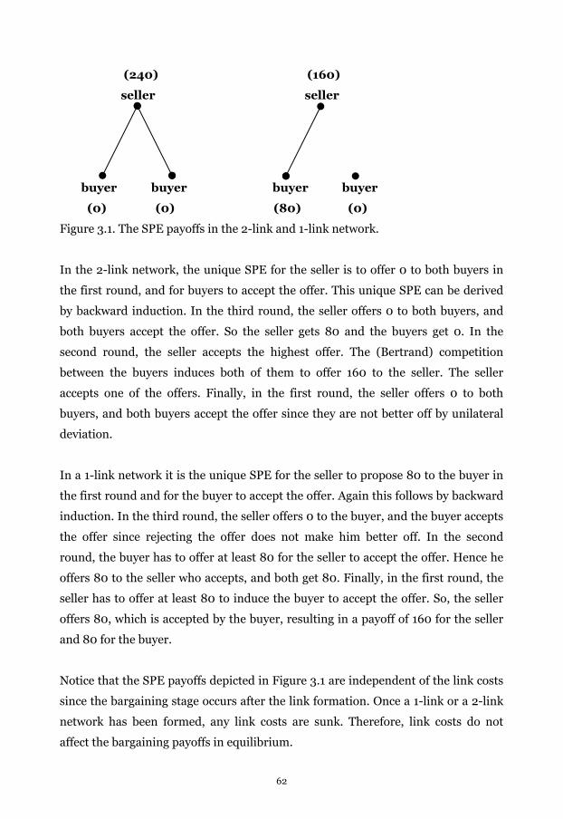
(240) (160)
seller seller
buyer buyer buyer buyer
(0) (0) (80) (0)
Figure 3.1. The SPE payoffs in the 2-link and 1-link network.
In the 2-link network, the unique SPE for the seller is to offer 0 to both buyers in
the first round, and for buyers to accept the offer. This unique SPE can be derived
by backward induction. In the third round, the seller offers 0 to both buyers, and
both buyers accept the offer. So the seller gets 80 and the buyers get 0. In the
second round, the seller accepts the highest offer. The (Bertrand) competition
between the buyers induces both of them to offer 160 to the seller. The seller
accepts one of the offers. Finally, in the first round, the seller offers 0 to both
buyers, and both buyers accept the offer since they are not better off by unilateral
deviation.
In a 1-link network it is the unique SPE for the seller to propose 80 to the buyer in
the first round and for the buyer to accept the offer. Again this follows by backward
induction. In the third round, the seller offers 0 to the buyer, and the buyer accepts
the offer since rejecting the offer does not make him better off. In the second
round, the buyer has to offer at least 80 for the seller to accept the offer. Hence he
offers 80 to the seller who accepts, and both get 80. Finally, in the first round, the
seller has to offer at least 80 to induce the buyer to accept the offer. So, the seller
offers 80, which is accepted by the buyer, resulting in a payoff of 160 for the seller
and 80 for the buyer.
Notice that the SPE payoffs depicted in Figure 3.1 are independent of the link costs
since the bargaining stage occurs after the link formation. Once a 1-link or a 2-link
network has been formed, any link costs are sunk. Therefore, link costs do not
affect the bargaining payoffs in equilibrium.
62

Given the SPE payoffs of the bargaining stage, the Nash equilibria of the link
formation stage depend on the cost of a link. When links are costless, all networks
are Nash equilibria. No player has an incentive to unilaterally break a link, in
neither the 1-link nor the 2-link network. Moreover, as long as the seller believes
that a buyer will not offer a link, the seller is indifferent between offering and not
offering a link to that buyer. The same holds for the buyers. Hence, any network is a
Nash equilibrium. When the link costs are 40, the empty network and the two 1-
link networks are Nash equilibria of the link formation stage. The 2-link network,
however, is not a Nash equilibrium because a buyer has an incentive to unilaterally
delete the link with the seller. In the 2-link network the link costs are 40, whereas
the buyer’s bargaining payoff is zero. Hence, in the 2-link network, a buyer
improves his payoffs from -40 to 0 by not forming a link. Notice that there is also a
mixed strategy equilibrium if the link costs are 40. Both buyers in the mixed
strategy equilibrium offer the seller a link with probability .5, while the seller offers
a link to both buyers. The expected payoffs in this equilibrium are 100 and 0 for the
seller and buyers, respectively. Notice that the 1-link network equilibrium (weakly)
Pareto dominates the mixed strategy equilibrium.
We also examined trembling hand perfect (THP) equilibrium given the SPE payoffs
of the bargaining stage. THP equilibrium eliminates weakly dominated strategies
and is a refinement of Nash equilibrium. When links are costless, only the 2-link
network is a THP equilibrium because the seller weakly prefers to offer links to
both buyers and both buyers are weakly better off by offering a link to the seller.
When the link costs are 40, only the 1-link networks are THP. The seller offers a
link to both buyers, but only one of the buyers reciprocates. The empty network is
not a THP since the seller weakly prefers to offer two links to the buyers. Given that
one buyer does not offer a link to the seller, the other buyer is better off by offering
a link to the seller. The mixed strategy equilibrium in which the seller offers two
links and both buyers offer a link with probability .5 is also THP.
63
Hypotheses
We formulate the standard theoretical predictions into four hypotheses.
Throughout the hypotheses and the results section, the theoretical payoff
predictions from the bargaining stage of the game are based on the SPE
predictions, and the link formation predictions are based on the THP equilibrium
predictions, unless otherwise stated.
H1. The effect of the link costs on link formation.
1a. The seller offers two links irrespective of the link costs.
The seller offers two links irrespective of whether the link costs are 0 or 40
since offering two links is a weakly dominating strategy.
1b. The buyers are less likely to offer a link when link costs are 40.
If link costs are 0, both buyers offer a link to the seller. If the link costs are
40, only one buyer offers a link to the seller, or both do so with probability
0.5.
1c. The 2-link network forms less often when link costs are 40.
The 2-link network is both a Nash and a THP equilibrium when the link
costs are 0, but the 2-link network is not a Nash and hence not a THP
equilibrium when the link costs are 40. Moreover, the only pure THP
equilibria for the cost 0 and cost 40 cases are the 2-link and 1-link network,
respectively.
H2. The effect of competition on bargaining.
2a. The first round offer of the seller is higher in the 1-link network than in the
2-link network.
If there are two links, the seller offers 0 to the buyers in the first round of
the bargaining stage; when there is one link, the seller offers 80 to the
linked buyer.
2b. Buyers reject higher offers in the first round in the 1-link network than in
the 2-link network.
64
Both buyers accept any offer the seller makes in the first round in the 2-link
network; in a 1-link network, however, the buyer rejects any offer less than
80.
H3. The effect of the link costs on bargaining.
3a. Offers do not depend on the link costs.
Since the bargaining stage occurs after the link formation, when the players
are in the bargaining stage the link costs have already been incurred, i.e.,
the costs are sunk. As a result, conditional on the network that forms, the
offers in the bargaining stage are independent of the link costs.
3b. Rejecting an offer does not depend on the link costs.
The decision to accept or reject an offer is not affected by the link costs
since the link costs have been incurred once the bargaining stage is
reached.
H4. The effect of the link costs on payoffs.
4a. The seller is better off if there are no link costs.
If the link costs are zero the 2-link network is formed and the seller's net
payoff is 240. If the link costs are 40 and the 1-link network forms the
seller’s net payoff is 120 (160–40), whereas the seller’s expected payoff in
the mixed strategy equilibrium is .25×240 + .5×120 +.25×0 = 120 as well.
4b. The buyers are better off if there are link costs.
If there are no link costs, both buyers earn zero, since a 2-link network
forms. If the link costs are 40 and a 1-link network forms the linked buyer
earns 40 (80–40) and the other buyer earns zero, whereas their expected
payoff in the mixed strategy equilibrium equals .25×–40 + .5×0 +.25×40 =
0. Assuming that not all buyers play the mixed strategy equilibrium, the
buyer’s net payoff is higher if the link costs are 40 than if the link costs are
zero.
65
Alternative Theoretical Predictions
The experimental literature on bargaining indicates that people often do not
behave as predicted by standard theory. There exists growing evidence that people
exhibit social preferences (e.g., Camerer, 2003). In this section we show that social
preferences might lead the link costs to have an effect on the bargaining outcomes
contrary to the Hypotheses 3. In particular, we examine the predictions of
inequality aversion (Fehr and Schmidt, 1999), and equity theory (Homans, 1961,
Selten, 1978).
The model by Fehr and Schmidt (1999) assumes that a player’s utility decreases in
the absolute difference between his own payoff and the payoffs of other players.
The link costs might affect the difference between players' payoffs which in return
affects the bargaining outcomes. It is tedious but straightforward to derive the SPE
predictions for the bargaining stage with inequality averse players. The analysis
reveals that given a certain assumption the sunk link costs affect the bargaining
strategies25. In particular, when a 1-link network forms a seller makes a lower offer
to the buyer if there are link costs compared to the case without link costs. If the
link costs are 40, the buyer in the link accepts lower offers since he dislikes the fact
that his payoff from rejecting an offer (-40) is lower than the payoff of the other
buyer (0). Anticipating this, the seller offers less to the buyer in the cost 40 case
than in the case without link costs. Interestingly, link costs have no impact on the
bargaining outcome if a 2-link network is formed. The reason is that competition
induces the buyers to offer the whole pie to the seller in the second round which in
return results in the buyers accepting any offer of the seller in the first round
irrespective of the link costs. Consequently the seller offers zero to the buyers in
both cases.
25 The result relies on the assumption that the seller does not have a strong dislike for
disadvantageous inequality. To be precise, in the standard notation of the Fehr Schmidt
model, link costs affect bargaining if β < 2/3. Fehr and Schmidt suggest that this assumption
is reasonable for a vast majority of people.
66
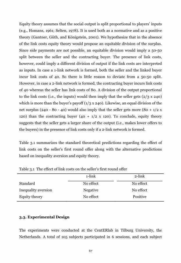
Equity theory assumes that the social output is split proportional to players' inputs
(e.g., Homans, 1961; Selten, 1978). It is used both as a normative and as a positive
theory (Gantner, Güth, and Königstein, 2001). We hypothesize that in the absence
of the link costs equity theory would propose an equitable division of the surplus.
Since side payments are not possible, an equitable division would imply a 50-50
split between the seller and the contracting buyer. The presence of link costs,
however, could imply a different division of output if the link costs are interpreted
as inputs. In case a 1-link network is formed, both the seller and the linked buyer
incur link costs of 40. So there is little reason to deviate from a 50-50 split.
However, in case a 2-link network is formed, the contracting buyer incurs link costs
of 40 whereas the seller has link costs of 80. A division of the output proportional
to the link costs (i.e., the inputs) would then imply that the seller gets (2/3 x 240)
which is more than the buyer’s payoff (1/3 x 240). Likewise, an equal division of the
net surplus (240 - 80 - 40) would also imply that the seller gets more (80 + 1/2 x
120) than the contracting buyer (40 + 1/2 x 120). To conclude, equity theory
suggests that the seller gets a larger share of the output (i.e., makes lower offers to
the buyers) in the presence of link costs only if a 2-link network is formed.
Table 3.1 summarizes the standard theoretical predictions regarding the effect of
link costs on the seller's first round offer along with the alternative predictions
based on inequality aversion and equity theory.
Table 3.1 The effect of link costs on the seller’s first round offer
1-link 2-link
Standard No effect No effect
Inequality aversion Negative No effect
Equity theory No effect Positive
3.3. Experimental Design
The experiments were conducted at the CentERlab in Tilburg University, the
Netherlands. A total of 105 subjects participated in 6 sessions, and each subject
67

participated only once. Subjects were recruited through email lists of students
interested in participating in experiments. There were in total 48 subjects in 3
sessions in the cost-0 treatment, and 57 subjects in 3 sessions in the cost-40
treatment. Subjects were at tables separated by partitions, such that they could not
see other participants’ screens but could see the experimenters in front of the room.
Sessions lasted between 90 and 150 minutes, and average earnings were
approximately 18.60 Euros including a show-up fee of 7.5 Euros.
First, written instructions were given to the participants and read out loud by the
experimenter. A copy of the instructions is included in Appendix 3A. It was
explained in the instructions that each group consisted of 3 players who were
randomly selected at the beginning of the experiment and that the group
composition stayed the same throughout the experiment. Subjects had no way of
knowing which of the other participants were in their group. In the instructions
and the experiment, the sellers were denoted as Player 1, and buyers were denoted
as Player 2 or Player 3. Player roles remained fixed throughout the experiment. The
game was explained as consisting of two parts: the first being about offering links
to other players and the second about sharing an amount of points. Subjects were
informed that the task would be repeated for 30 periods and that their final
earnings comprised of the total points they earned in the experiment converted at a
rate of 0.5 (0.7) Eurocents per point in the cost-0 (40) treatment plus the show up
fee. In the cost-40 treatment, it was emphasized that offering a link is not costly,
but that if a link is formed players who have the link each pay 40 points. After the
instructions were finished, subjects played one practice period in order to
familiarize them with the procedure and the screens. Subjects’ understanding of the
task was then assessed by asking them 3 questions to answer at their own pace.
Their answers were checked one by one and when necessary the task and the payoff
structure were explained again privately.
The experiment was programmed and conducted with the software z-Tree
(Fischbacher 2007).26 Each period started with a screen with the three boxes with
26 The program of the experiment is available from the authors upon request.
68
labels 1, 2, and 3, representing the players of the group. An example of the subject
screen is contained in the instructions of the experiment in Appendix 3A. A player's
own box was always presented on top of the screen. Players simultaneously decided
with whom to link, and they offered a link by clicking on the box of another player.
Buyers could not link to each other. Subjects saw an arrow pointing to the other
player's box when they clicked, and it was possible to undo the link offer by clicking
again. When the players moved to the next screen27, a line between two players on
the screen informed them about the links that formed. If a link was offered
unilaterally this was indicated with an arrow pointing to the other player.
If one link or two links were formed, the group proceeded to the bargaining stage in
which the seller offered a share between 0 and 240 points to the linked buyer or
buyers. If there were two links, the offers could be different for the two buyers.
Then, buyers were informed about the offer or offers that the seller made, and
buyers simultaneously decided whether to accept or reject the offer. If an offer was
accepted, the bargaining ended and the offer was implemented. If both buyers
accepted the offer, one of them was randomly chosen by the computer for the
payoff realisation. If both buyers rejected the seller’s offer, the group proceeded to
the second round of bargaining in which the buyer(s) offered a share between 0 and
160 to the seller. If the seller rejected the offer(s), they proceeded to the third and
final round, in which the seller offered a share between 0 and 80 to the buyer(s).
After each bargaining round, all players were informed about the acceptance and
rejection decisions of their group members even when they did not have a link. At
the end of bargaining, the players were informed about their own payoff in that
period, the group members’ payoffs in that period, and their own cumulative
payoffs. In the cost-40 treatment, their total payoff was the amount of points from
an agreement minus the link costs. Note that players could earn negative payoffs in
this treatment. All groups in a session started each period at the same time. Thus it
was not possible to identify one’s group members at any point of the experiment. At
27 The subjects moved to the next phase of the experiment when all group members pressed
the OK button. Also, each screen had a binding time limit of 180 seconds in the first 5
periods, and 60 seconds in the later periods.
69

the end of the experiment participants were paid privately and separately in an
adjacent room.
3.4. Results
In this section we discuss the experimental results. The results are organised
parallel to the hypotheses stated in Section 3.2.28
Effect of link costs on link formation
Result 1a. The hypothesis that the seller offers two links irrespective of the link
costs was rejected.
Table 3.2 depicts the average link offers per period as a function of costs and player
role. The second column of the table is the average number of links the seller
offered to each buyer per period. The third column states the average number of
links each buyer offered to the seller. The p-values from the comparison of the link
offers of the seller and the buyers within each treatment are stated in the last
column. Finally the last row shows the p-values from the comparison of the link
offers across the two treatments.
In the cost-0 treatment the seller offered an average of 0.87 links to each buyer per
period, which was significantly more than the average 0.61 links to each buyer in
the cost-40 treatment. So, contrary to the standard theoretical prediction, the seller
offered less than two links in both cost treatments, and the number of links offered
by the seller was significantly lower if there were link costs.
28 Unless stated otherwise, statistics treat a group of one seller and two buyers interacting
over 30 periods as one independent observation. This means that we have 16 independent
observations in the cost-0 treatment and 19 independent observations in the cost-40
treatment. The p-values reported for between-treatment comparisons are based on the
Mann-Whitney test; p-values reported for within-treatment comparisons are based on the
Wilcoxon matched-pairs signed-ranks test. We use a one-sided (two-sided) test when the
hypothesis is (is not) directional.
70
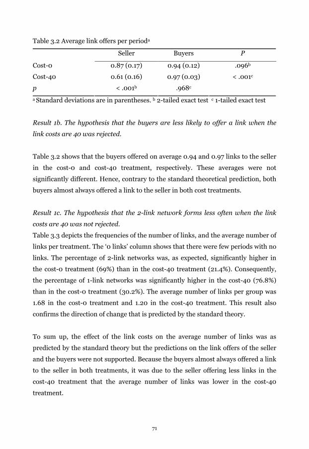
Table 3.2 Average link offers per perioda
Seller Buyers P
Cost-0 0.87 (0.17) 0.94 (0.12) .096b
Cost-40 0.61 (0.16) 0.97 (0.03) < .001c
p < .001b .968c
a Standard deviations are in parentheses. b 2-tailed exact test c 1-tailed exact test
Result 1b. The hypothesis that the buyers are less likely to offer a link when the
link costs are 40 was rejected.
Table 3.2 shows that the buyers offered on average 0.94 and 0.97 links to the seller
in the cost-0 and cost-40 treatment, respectively. These averages were not
significantly different. Hence, contrary to the standard theoretical prediction, both
buyers almost always offered a link to the seller in both cost treatments.
Result 1c. The hypothesis that the 2-link network forms less often when the link
costs are 40 was not rejected.
Table 3.3 depicts the frequencies of the number of links, and the average number of
links per treatment. The ‘0 links’ column shows that there were few periods with no
links. The percentage of 2-link networks was, as expected, significantly higher in
the cost-0 treatment (69%) than in the cost-40 treatment (21.4%). Consequently,
the percentage of 1-link networks was significantly higher in the cost-40 (76.8%)
than in the cost-0 treatment (30.2%). The average number of links per group was
1.68 in the cost-0 treatment and 1.20 in the cost-40 treatment. This result also
confirms the direction of change that is predicted by the standard theory.
To sum up, the effect of the link costs on the average number of links was as
predicted by the standard theory but the predictions on the link offers of the seller
and the buyers were not supported. Because the buyers almost always offered a link
to the seller in both treatments, it was due to the seller offering less links in the
cost-40 treatment that the average number of links was lower in the cost-40
treatment.
71
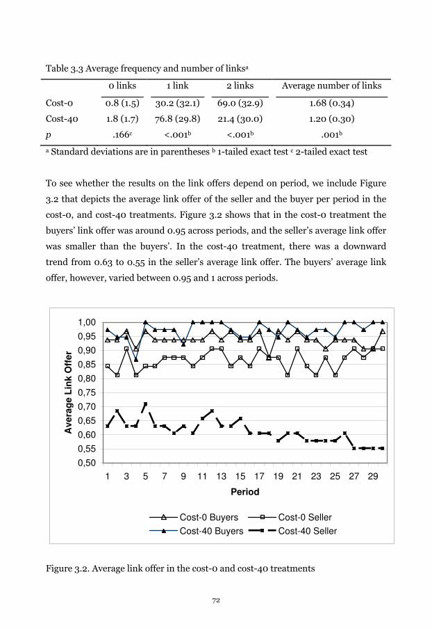
Table 3.3 Average frequency and number of linksa
0 links 1 link 2 links Average number of links
Cost-0 0.8 (1.5) 30.2 (32.1) 69.0 (32.9) 1.68 (0.34)
Cost-40 1.8 (1.7) 76.8 (29.8) 21.4 (30.0) 1.20 (0.30)
p .166c <.001b <.001b .001b
a Standard deviations are in parentheses b 1-tailed exact test c 2-tailed exact test
To see whether the results on the link offers depend on period, we include Figure
3.2 that depicts the average link offer of the seller and the buyer per period in the
cost-0, and cost-40 treatments. Figure 3.2 shows that in the cost-0 treatment the
buyers’ link offer was around 0.95 across periods, and the seller’s average link offer
was smaller than the buyers’. In the cost-40 treatment, there was a downward
trend from 0.63 to 0.55 in the seller’s average link offer. The buyers’ average link
offer, however, varied between 0.95 and 1 across periods.
0,50
0,55
0,60
0,65
0,70
0,75
0,80
0,85
0,90
0,95
1,00
1 3 5 7 9 11 13 15 17 19 21 23 25 27 29
Period
Av
era
ge
Lin
k O
ffe
r
Cost-0 Buyers Cost-0 Seller
Cost-40 Buyers Cost-40 Seller
Figure 3.2. Average link offer in the cost-0 and cost-40 treatments
72
To analyze whether the failure of the prediction that the seller always offers two
links was confined to some groups, we made descriptive analyses on the link offers
at the group level. We found that the variance of behavior of the sellers between
and within treatments was high whereas the buyers’ behavior did not noticeably
differ. In the cost-0 treatment 10 out of 16 sellers offered two links in at least 80%
of the periods, but only two out of 19 sellers did so in the cost-40 treatment.
Likewise, two out of 16 sellers in the cost-0 treatment offered one link in at least
80% of the periods whereas the majority (12 out of 19) of sellers did so in the cost-
40 treatment. To conclude, most sellers offered two links in the cost-0 treatment,
whereas the majority of sellers offered one link in the cost-40 treatment. Contrary
to the sellers, the behavior of the buyers was similar in the two cost treatments.
Most buyers offered a link in at least 80% of the periods; 30 out of 32 buyers in the
cost-0 treatment, and all 38 buyers in the cost-40 treatment.
Finally, the only two groups in the cost-40 treatment in which the seller offered two
links in most periods (27 and 30 periods, respectively) showed that, even though
there existed monetary incentives to do so, the buyers did not coordinate on
forming only one link with the seller. In both groups buyers always offered a link
except in one period in the second group and buyers on average had a negative
payoff. Hence both buyers in the first group and at least one of the buyers in the
second group did not try to coordinate.
Effect of competition on bargaining
Result 2a. The hypothesis that the first round offer of the seller is higher in the 1-
link network than in the 2-link network was not rejected.
In Table 3.4 the average offers of the first, second, and third rounds conditional on
the number of links are depicted. The last column shows the p-values of the
comparison of the first round offers of the 1-link network with the first round offers
of the 2-link network. The average offer in the first round was significantly higher
in the 1-link than in the 2-link network for both cost treatments; 75.6 vs. 65.13 and
95.15 vs. 60.41, for the cost-0 and cost-40 treatments, respectively. Hence, as
73

predicted, competition between the buyers reduced the seller's offer. Nevertheless,
the point prediction was quite far off the mark for the 2-link case. The seller was
predicted to offer 0 in the first round, whereas the observed offer was above 60 in
both treatments. Too few observations were available to test corresponding
hypotheses on the second and third round offers.29 Note from Table 3.4, however,
that the direction of the differences were in line with the theoretical predictions.
Table 3.4 Average offer per round a, b
First Second Third
1 link 2 links 1 link 2 links 1 link 2 links p (first)c
Cost-0
75.60
(21.10)
N=15
65.13
(25.20)
N=14
66.96
(18.42)
N=12
84.80
(11.93)
N=4
23.60
(12.71)
N=10
11.25 (1.77)
N=2
<.001
N=13
Cost-40
95.15
(22.26)
N=19
60.41
(21.29)
N=11
59.89
(13.53)
N=16
75.18
(19.75)
N=9
26.49
(14.80)
N=13
20.00
(15.00)
N=3
.001
N=11
p d .023 .809 .245 .414 .633 .800
a Standard deviations are in parentheses b The number of observations are
indicated with N c 1-tailed exact test. d 2-tailed exact test
Result 2b. The hypothesis that the buyers reject higher offers in the first round in
the 1-link network than in the 2-link network was not rejected.
We ran a logistic regression analysis to analyse the effect of the number of links on
the acceptance decisions of the buyers in the first round, controlling for the offer of
the seller. We report the results of two models in Table 3.5. Apart from the link
costs, the number of links, the interaction between link costs and number of links,
and the period number, Model 1 also includes interaction effects between these
29 In the cost-0 treatment, there were four groups that had data on both 1-link and 2-link
second round offers, and in the cost-40 treatment, there were eight. In the cost-0 treatment,
there were two groups that had data on both 1-link and 2-link third round offers, and in the
cost-40 treatment, there was one.
74
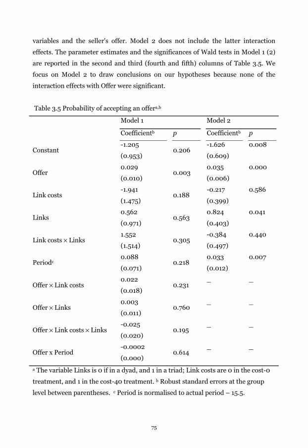
variables and the seller's offer. Model 2 does not include the latter interaction
effects. The parameter estimates and the significances of Wald tests in Model 1 (2)
are reported in the second and third (fourth and fifth) columns of Table 3.5. We
focus on Model 2 to draw conclusions on our hypotheses because none of the
interaction effects with Offer were significant.
Table 3.5 Probability of accepting an offera,b
Model 1 Model 2
Coefficientb p Coefficientb p
Constant -1.205
(0.953) 0.206
-1.626
(0.609)
0.008
Offer 0.029
(0.010) 0.003
0.035
(0.006)
0.000
Link costs -1.941
(1.475) 0.188
-0.217
(0.399)
0.586
Links 0.562
(0.971) 0.563
0.824
(0.403)
0.041
Link costs × Links 1.552
(1.514) 0.305
-0.384
(0.497)
0.440
Periodc 0.088
(0.071) 0.218
0.033
(0.012)
0.007
Offer × Link costs 0.022
(0.018) 0.231
_ _
Offer × Links 0.003
(0.011) 0.760
_ _
Offer × Link costs × Links -0.025
(0.020) 0.195
_ _
Offer x Period -0.0002
(0.000) 0.614
_ _
a The variable Links is 0 if in a dyad, and 1 in a triad; Link costs are 0 in the cost-0
treatment, and 1 in the cost-40 treatment. b Robust standard errors at the group
level between parentheses. c Period is normalised to actual period – 15.5.
75
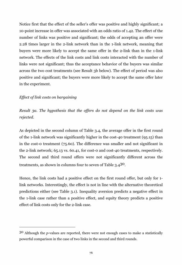
Notice first that the effect of the seller's offer was positive and highly significant; a
10-point increase in offer was associated with an odds ratio of 1.42. The effect of the
number of links was positive and significant; the odds of accepting an offer were
2.28 times larger in the 2-link network than in the 1-link network, meaning that
buyers were more likely to accept the same offer in the 2-link than in the 1-link
network. The effects of the link costs and link costs interacted with the number of
links were not significant; thus the acceptance behavior of the buyers was similar
across the two cost treatments (see Result 3b below). The effect of period was also
positive and significant; the buyers were more likely to accept the same offer later
in the experiment.
Effect of link costs on bargaining
Result 3a. The hypothesis that the offers do not depend on the link costs was
rejected.
As depicted in the second column of Table 3.4, the average offer in the first round
of the 1-link network was significantly higher in the cost-40 treatment (95.15) than
in the cost-0 treatment (75.60). The difference was smaller and not significant in
the 2-link network; 65.13 vs. 60.41, for cost-0 and cost-40 treatments, respectively.
The second and third round offers were not significantly different across the
treatments, as shown in columns four to seven of Table 3.430.
Hence, the link costs had a positive effect on the first round offer, but only for 1-
link networks. Interestingly, the effect is not in line with the alternative theoretical
predictions either (see Table 3.1). Inequality aversion predicts a negative effect in
the 1-link case rather than a positive effect, and equity theory predicts a positive
effect of link costs only for the 2-link case.
30 Although the p-values are reported, there were not enough cases to make a statistically
powerful comparison in the case of two links in the second and third rounds.
76

To check whether the effect of link costs is perhaps due to confusion and is reduced
by learning we plot the average first round offer for 10 different segments of
periods (1-3, 4-6,…, 27-30). Figure 3.3 depicts the average first round offer in the 1-
link and 2-link networks for both cost treatments. For the 1-link networks, the
average offer was consistently higher in the cost-40 treatment, with a minimum
difference higher than 10.29 points for all period segments. Thus, Figure 3.3
supports the result that the offers were significantly different in the 1-link networks
across cost treatments. Consider now the offers in the 2-link networks in the two
cost treatments. Even though the offers were consistently higher in the cost-0
treatment, the difference between the treatments was not statistically significant in
any of the ten segments. Moreover, there was no evidence that over the periods the
offers were getting closer to the theoretical prediction that the seller offers zero.
50
55
60
65
70
75
80
85
90
95
100
3 6 9 12 15 18 21 24 27 30
Period
Av
era
ge
Fir
st
Ro
un
d O
ffe
r
Cost-0 One Link Cost-40 One Link
Cost-0 Two Links Cost-40 Two Links
Figure 3.3. The average first round offers if there is one or two links
77

Result 3b. The hypothesis that rejecting an offer does not depend on the link costs
was not rejected.
Table 3.5 above shows the logistic regression results on the acceptance probability
of the offer. The effect of link costs on the probability of accepting an offer was,
although negative, not significant. The interaction effect between link costs and
number of links was negative, indicating that link costs had a smaller effect in case
of 2 links, but this effect was not significant. To sum up, there was a significant
positive effect of the link costs on the seller's first round offer, but only in case a 1-
link network formed, and link costs did not have a significant effect on the buyers’
bargaining, that is, the acceptance probability of an offer.
Effect of link costs on payoffs
Result 4a. The hypothesis that the seller is better off if there are no link costs is not
rejected.
Table 3.6 shows the average net payoffs of the seller and the buyer as well as the
average 1-link and 2-link payoffs. The p-values in the fifth column correspond to
the tests comparing the earnings of the sellers in the 1-link network to the earnings
of the seller in the 2-link network within each cost treatment. Likewise, the p-
values in the last column correspond to the tests comparing the earnings of the
buyers.
The seller earned on average 151.58 in the cost-0 treatment, which was significantly
higher than the average earning of 82.14 in the cost-40 treatment. Note that the
average earning of the seller in the cost-0 treatment was almost 89 points less than
the theoretical prediction, and in the cost-40 treatment it was 38 points less. The
seller also earned less than the predicted 160 points in the 1-link network.
78
Table 3.6 Average net payoffs per period a, b
Seller Buyers
Average 1 link 2 links pc Average 1 link 2 links pc
Cost-0 151.48
(23.44)
113.57
(36.98)
N=15
164.99
(22.82)
N=14
<.001
N=13
34.60
(10.46)
37.02
(11.52)
N=15
33.33
(11.99)
N=14
.133
N=13
Cost-40 82.14
(12.45)
80.09
(27.73)
N=19
75.87
(24.72)
N=11
.700
N=11
18.12
(14.09)
27.97
(14.03)
N=19
-7.24
(9.53)
N=11
.001
N=11
pc <.001 .002 <.001 <.001 .007 <.001
a Standard deviations are in parentheses b The number of observations are
indicated with N c 1-tailed exact test.
There were three reasons why the seller’s earnings were substantially lower than
the theoretical predictions. First, contrary to the theoretical predictions, 1-link
networks formed in as much as 30% of the cases in the cost-0 treatment (see Table
3.3), which decreased the seller payoffs. Second, sellers’ first round offers were
higher than predicted if there were two links. In both treatments, sellers offered
more than 60 in the first round, whereas they were predicted to offer 0. The third
reason was the buyers’ rejection of the first round offers of the seller. The
cumulative acceptance frequency of the offers is depicted in Table 3.7. It can be
seen that in the cost-0 treatment in the 1-link network, 42 percent of the offers
were rejected in the first round whereas in the 2-link network both buyers rejected
the seller’s offer in only 7 percent of the cases. In the cost-40 treatment, however,
the percentage of rejections in the first round were similar in both 1-link and 2-link
cases; 22 percent in the 1-link network and 21 percent in the 2-link network. Thus,
the seller’s payoff from 1-link networks in the cost-0 treatment was substantially
lessened due to disagreements.
79
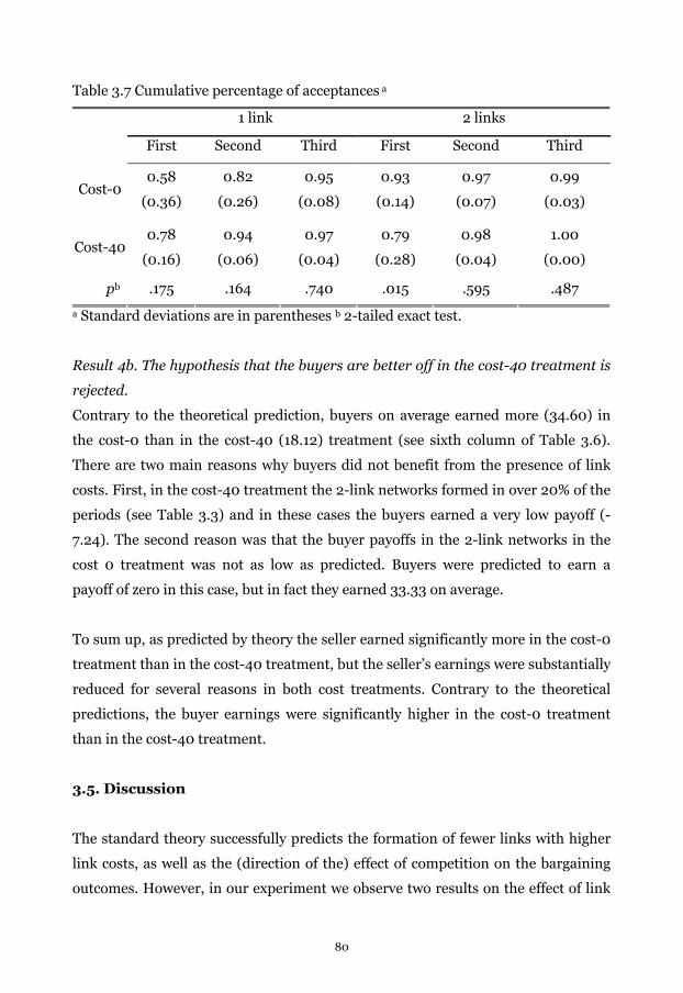
Table 3.7 Cumulative percentage of acceptances a
1 link 2 links
First Second Third First Second Third
Cost-0 0.58
(0.36)
0.82
(0.26)
0.95
(0.08)
0.93
(0.14)
0.97
(0.07)
0.99
(0.03)
Cost-40 0.78
(0.16)
0.94
(0.06)
0.97
(0.04)
0.79
(0.28)
0.98
(0.04)
1.00
(0.00)
pb .175 .164 .740 .015 .595 .487
a Standard deviations are in parentheses b 2-tailed exact test.
Result 4b. The hypothesis that the buyers are better off in the cost-40 treatment is
rejected.
Contrary to the theoretical prediction, buyers on average earned more (34.60) in
the cost-0 than in the cost-40 (18.12) treatment (see sixth column of Table 3.6).
There are two main reasons why buyers did not benefit from the presence of link
costs. First, in the cost-40 treatment the 2-link networks formed in over 20% of the
periods (see Table 3.3) and in these cases the buyers earned a very low payoff (-
7.24). The second reason was that the buyer payoffs in the 2-link networks in the
cost 0 treatment was not as low as predicted. Buyers were predicted to earn a
payoff of zero in this case, but in fact they earned 33.33 on average.
To sum up, as predicted by theory the seller earned significantly more in the cost-0
treatment than in the cost-40 treatment, but the seller’s earnings were substantially
reduced for several reasons in both cost treatments. Contrary to the theoretical
predictions, the buyer earnings were significantly higher in the cost-0 treatment
than in the cost-40 treatment.
3.5. Discussion
The standard theory successfully predicts the formation of fewer links with higher
link costs, as well as the (direction of the) effect of competition on the bargaining
outcomes. However, in our experiment we observe two results on the effect of link
80

costs that cannot be explained by standard theory: (i) the seller determines which
type of network is formed, and (ii) the offers of the seller are significantly affected
by the presence or absence of link costs.
Theory predicts that in both cost treatments the seller offers links to both buyers,
and that (on average) only one buyer offers a link to the seller in the cost-40
treatment. However, the formation of a 1-link network was mostly due to the seller,
since both buyers almost always offered a link to the seller. Why did the sellers not
offer two links more often in the cost-40 treatment? The reason for this is simply
that it was not profitable to do so on average. Theoretically, having two links rather
than one link is predicted to increase the seller's net payoff from 120 (=160-40) to
160 (=240-80). As can be seen in Table 3.6, however, in the experiment the average
net payoff to the seller is actually lower in a 2-link network (75.87) than in a 1-link
network (80.09). Although, a seller usually gets a larger higher share of the surplus
with two links, this is not enough to compensate for the extra link costs.
The second main result that is not in line with the standard model is that the sellers
on average offered 20 points more to the buyer in the cost-40 treatment (96) than
in the cost-0 treatment (76) in a 1-link network. Interestingly, this finding cannot
be explained by inequality aversion or equity theory either. Below we examine four
potential explanations. The first two are 'static' while the last two rely on the game
being repeated.
First, in line with the fairness model by Bolton and Ockenfels (2000), we explored
the assumption that players care about relative payoff shares rather than absolute
payoff differences (as in Fehr and Schmidt, 1999). This may matter for the
predicted impact of link costs. If two sides of a link have to pay link costs of 40,
their absolute payoff difference does not change, but their relative payoff shares
may. To illustrate, consider a 1-link network in which the seller makes a first round
offer of 80 to the buyer. In case the link costs are 0, this offer gives the buyer a
share of 1/3 (80/240) of the total payoff. In case the link costs are 40, however, the
same offer would give the buyer a share of only 1/4 (40/160). So, in order to give
the buyer the same net payoff share, the seller would have to increase her offer (as
81

in fact we observe in the experiment). In a 2-link network this effect is mitigated (or
even reversed) by the fact that the seller has to pay the link costs twice. To examine
this argument more generally, it would be useful to apply the model by Bolton and
Ockenfels (2000). This model, however, is only defined for games with non-
negative payoffs and it is not obvious how to adjust the model such that its allows
for negative payoffs. We have experimented with several alternative models, but
the results are quite sensitive to the exact specification.
Second, it has been suggested that Prospect Theory (PT) might be able to explain
the impact of sunk costs. Upon paying the cost of establishing a link, players may
perceive to be 'in the domain of losses', which may make them more prone to take
risks than in the case without link costs. Clearly, for PT to have bite there needs to
be some degree of (strategic) uncertainty in the game. A natural candidate to
incorporate such uncertainty is Quantal Response Equilibrium (QRE), which
assumes that players make errors, and are more likely to make errors with small
costs than errors with large costs (McKelvey and Palfrey, 1995, 1998). Note that the
link costs can affect QRE predictions only if the utility function is nonlinear or if it
incorporates loss aversion. We calculated the QRE predictions for the bargaining
game to examine whether it can predict the difference in the seller's offer across the
cost treatment. We assumed that all players had the same power value function
with loss aversion and the same risk parameter for losses and gains31. We found
that the 20 points difference in the seller’s first period offers in the 1-link network
between the cost-0 and cost-40 treatments could not be explained by QRE with any
parameter value combination. The maximum point difference was 11, but then
other predictions, like those on the absolute value of the offers and the net payoffs,
were substantially off the mark. So, although it is possible to predict an increase in
the first round offers using a combination of PT and QRE, there does not exist a
31 If x denotes the payoff, the utility of the subjects is u(x) = xα for nonnegative x, and u(x) =
–λ(–x)α for negative x, where α is the risk aversion parameter, and λ ≥ 1 measures loss
aversion. We computed all QRE using values of α between 0.5 to 1, values of λ between 1 and
5, and the rationality parameter ranging from 0 (random behavior) to infinity (full
rationality).
82

parameter combination such that average predicted behavior is close to that
observed in the experiment.
Third, there is substantial experimental evidence that agents tend to act fairer
towards another agent the more stable the relationship they are in. For example, in
Brown, Falk, and Fehr (2004) rents tend to be shared more equally when the
trading parties were contracting over longer periods of time. Therefore, a
reasonable hypothesis for our game is that on average a seller offered a larger share
of the pie to a buyer in the cost-40 treatment because typically they had more stable
bilateral relationships in this treatment than in the cost-0 treatment. To examine
this hypothesis we calculated the average number of periods that a 1-link
relationship between a seller and a buyer lasted in the two treatments. Indeed, we
found that 1-link relationships typically lasted longer in the cost-40 treatment (2.3
periods on average) than in the cost-0 treatment (1.4 periods on average).
However, there is no evidence that sellers made higher offers to the buyer when
their relationship lasted longer. Quite the contrary; on average a seller decreased
the offer to the buyer when the 1-link relationship proceeded from one period to the
next, and this was true for both treatments. Hence, we can reject the hypothesis
that sellers' offers in a 1-link relationship are higher in the cost-40 treatment than
in the cost-0 treatment because relationships on average lasted longer in the
former than in the latter treatment.
A final explanation for the effect of link costs on the seller's offer in the 1-link case
also relies on the game being repeated. The presence of linking costs reduces the
seller's bargaining power in a 1-link network in the cost-40 compared to the cost-0
treatment. If a 1-link network is formed in the cost-0 treatment, the implicit threat
by the seller to move to a 2-link network in the next period is very credible. Recall
from Table 3.2 that the buyers almost always offer a link, so essentially the seller
decides which network forms. This enables the seller to extract a relatively large
part of the pie in the 1-link network (larger than the SPE predictions); if the buyer
does not accept an offer, in the next period the seller can move to the 2-link
network in which the buyer can expect to get a lower payoff. In the cost-40
treatment, it is also feasible for the seller to move to a 2-link network, but such a
83

move is substantially less attractive as the seller has to pay the linking costs twice.
The implicit threat to move from a 1-link to a 2-link network in the next period is
less credible in the cost-40 treatment and as a result the seller has to offer a larger
share of the pie to the buyer.
Some empirical evidence is in line with this explanation. We investigated the rate at
which sellers moved from a 1-link network in period t to a 2-link network in period
t+1, in case the seller's offer was rejected by the buyer in the first round of period t.
We find that this rate is 0.429 (18/42) in the cost-0 and 0.143 (13/92) in the cost-
40 treatment. This suggests that the implicit threat to move to a 2-link network in
case the seller's offer was rejected in the 1-link network was executed more
frequently in the cost-0 treatment than in the cost-40 treatment.32 Moreover,
moving from a 1-link network to a 2-link network was considerably more profitable
for the seller in the cost-0 than the cost-40 treatment. On average, a seller
increased his payoffs from 110.7 to 172.5 when moving from a 1-link to a 2-link
network in the cost-0 treatment. In the cost-40 treatment, such a move increased
the seller's average payoff as well, from 62.1 to 84.1, but the increase is lower than
in the cost-0 treatment. These figures support the hypothesis that the presence of
linking costs reduced the bargaining power of the seller in the 1-link network as it
made the outside option less attractive.
3.6. Conclusion
In this paper we addressed two main questions regarding the effect of link costs on
networks. First, do link costs affect the competitiveness of networks? Second, do
link costs have a direct effect on the interaction within the network, independently
of the network that forms?
32 Note that this difference may be biased somewhat by the fact that there were more
switches for a 1-link to a 2-link network in the cost-0 treatment than in the cost-40
treatment overall.
84
To examine these questions we implemented a two-stage game between one seller
and two potential buyers. In the first stage, the seller decides whether to form one
or two links with the buyers and the buyers simultaneously decide whether to form
a link with the seller. In the second stage, and conditional on the network that was
formed in the first stage, the players engage in a three round alternating offer
bargaining with a shrinking surplus. The players bargain over the division of the
gains of trade, where at most one buyer can trade with the seller.
Regarding the first question, we find that link costs reduce the number of links as
the standard theory predicts. Without link costs, a competitive network is likely to
form in which the seller is linked to both buyers. The introduction of link costs
reduces the prevalence of competitive networks and the seller usually ends up
being linked to one buyer only. Moreover, as predicted, the competitiveness of the
network has a strong effect on the bargaining outcomes. The seller is able to extract
a significantly larger share of the surplus if he or she is linked to two buyers rather
than one, even though the difference is not as large as predicted by the standard
model based on full rationality and strict selfishness. Another notable finding is the
sellers do not employ the (theoretically dominant) strategy of offering two links
regardless of the link costs, whereas the buyers almost always offer a link to the
seller in both cost treatments. Consequently, sellers determine the network. Many
sellers offer only one link in the presence of link costs because they experience or
anticipate (correctly) that on average they do not earn more in the 2-link network
than in the 1-link network.
Second, we study whether the interaction in the network is affected by the costs of
link formation. Standard theory predicts that link costs do not affect the interaction
within the network, since network formation precedes the interaction in the
network. However, we find that link costs do influence bargaining outcomes if there
is one link, but not if there are two links. The presence of link costs significantly
increases sellers' offers in a dyad, while offers are not affected in a triad. This
finding is in contrast to the standard sunk cost argument. Several potentially
relevant models (inequality aversion, equity theory, prospect theory, quantal
response equilibrium) cannot account for this result either. We retain two
85

behavioral factors that can at least partially explain the impact of link costs on the
seller's offers. One rests on the assumption that players care about their relative
payoff shares (rather than about absolute payoff differences). The other
explanation is based on the fact that the seller’s bargaining power in the 1-link
network is higher in the cost-0 than in the cost-40 treatment because the
alternative, a 2-link network, is relatively more attractive in the former than in the
latter treatment.
In sum, the present paper shows that link costs play a dual role for markets and
other settings that require connections to be established between transacting
agents. Firstly, they shape the competitiveness (power distribution) of the network,
which in turn exerts a strong influence on the outcomes. Secondly, link costs have a
direct effect on the interaction within a network. Link costs cannot simply be
assumed to be sunk, once a network has formed. In other words, the interaction
within a network cannot simply be assumed to be independent from the formation
of the network.
86

Appendix 3A. Experimental Instructions for the Cost-0 Treatment
Introduction
Welcome to this experiment on decision making. We will first go through the
instructions together. Then there will be a practice period. After the practice period
the experiment will start. Talking is strictly forbidden during the experiment. If you
have a question, please raise your hand and I will come to your table to answer your
question.
The experiment will last about 2 hours. If you follow the instructions carefully you
can earn a considerable amount of money. During the experiment your earnings
will be denoted in points. After the experiment your earnings will be converted into
money at a rate of 1 point is 0.5 Eurocents. In addition, you will receive a show-up
fee of 7.5 Euros. Your earnings will be paid to you, privately and in cash,
immediately after the experiment.
Instructions for the experiment
In this experiment, you are in a group of 3 persons. Each person has her or his own
number; 1, 2, or 3. Your number is randomly determined at the beginning of the
practice period and it stays the same throughout the whole experiment. Also, the
composition of your group remains the same throughout the experiment. You will
not know who is in your group. You and your group members are referred to as
player 1, player 2 and player 3.
Your group faces the same task for 30 periods. The task has two parts. First, you
make a decision about whether to offer links to other players in your group or not.
Second, players who form a link to each other try to share an amount of points
between them.
In the first part a link is formed between two players if both of them offer a link to
each other. Player 1 can have two links; player 2 and 3 can have only one. Hence
player 2 and player 3 each have to decide whether they want to offer a link to player
1. Player 1 has to decide whether to offer a link to player 2 and whether to offer a
87
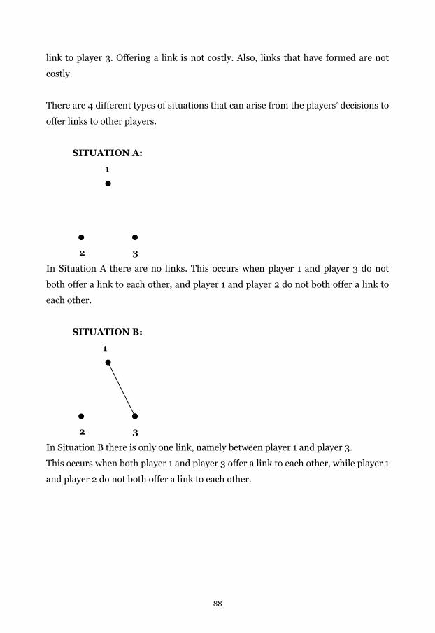
link to player 3. Offering a link is not costly. Also, links that have formed are not
costly.
There are 4 different types of situations that can arise from the players’ decisions to
offer links to other players.
SITUATION A:
1
2 3
In Situation A there are no links. This occurs when player 1 and player 3 do not
both offer a link to each other, and player 1 and player 2 do not both offer a link to
each other.
SITUATION B:
1
2 3
In Situation B there is only one link, namely between player 1 and player 3.
This occurs when both player 1 and player 3 offer a link to each other, while player 1
and player 2 do not both offer a link to each other.
88
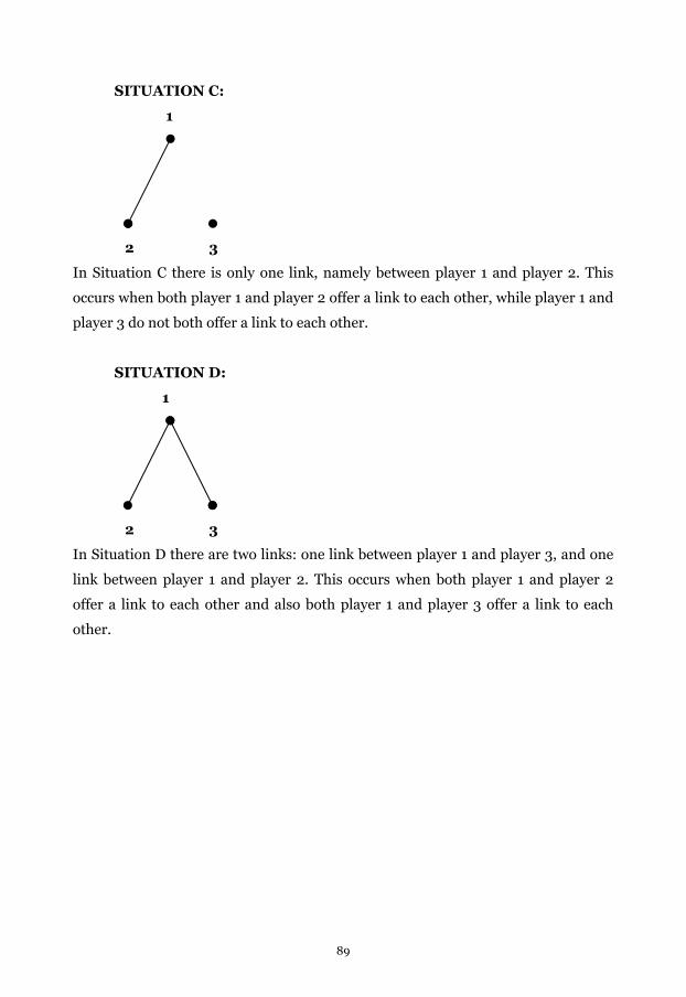
SITUATION C:
1
2 3
In Situation C there is only one link, namely between player 1 and player 2. This
occurs when both player 1 and player 2 offer a link to each other, while player 1 and
player 3 do not both offer a link to each other.
SITUATION D:
1
2 3
In Situation D there are two links: one link between player 1 and player 3, and one
link between player 1 and player 2. This occurs when both player 1 and player 2
offer a link to each other and also both player 1 and player 3 offer a link to each
other.
89
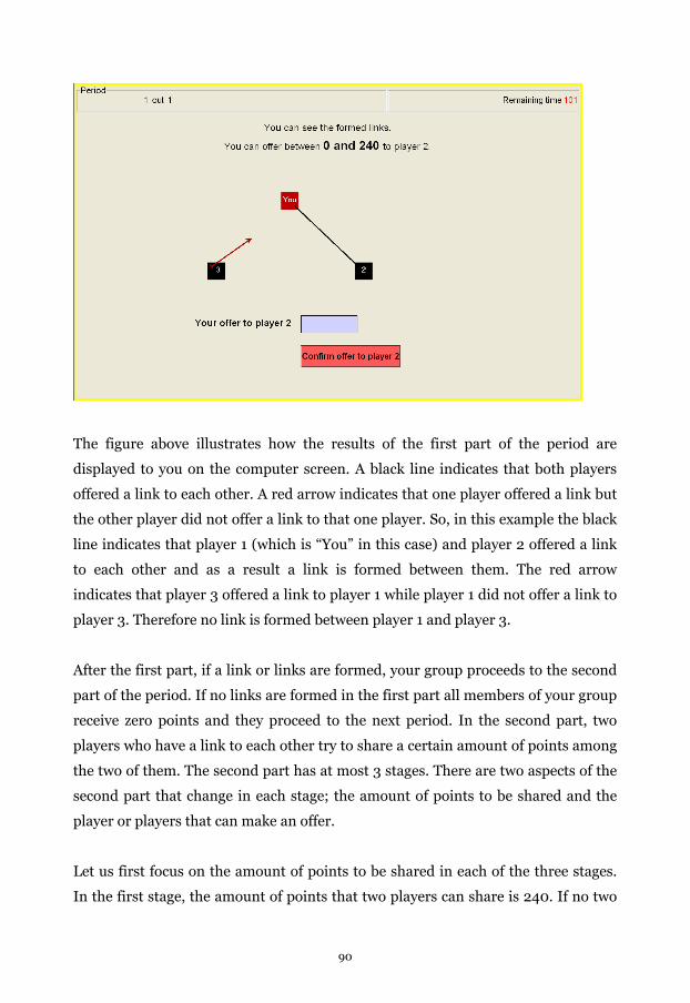
The figure above illustrates how the results of the first part of the period are
displayed to you on the computer screen. A black line indicates that both players
offered a link to each other. A red arrow indicates that one player offered a link but
the other player did not offer a link to that one player. So, in this example the black
line indicates that player 1 (which is “You” in this case) and player 2 offered a link
to each other and as a result a link is formed between them. The red arrow
indicates that player 3 offered a link to player 1 while player 1 did not offer a link to
player 3. Therefore no link is formed between player 1 and player 3.
After the first part, if a link or links are formed, your group proceeds to the second
part of the period. If no links are formed in the first part all members of your group
receive zero points and they proceed to the next period. In the second part, two
players who have a link to each other try to share a certain amount of points among
the two of them. The second part has at most 3 stages. There are two aspects of the
second part that change in each stage; the amount of points to be shared and the
player or players that can make an offer.
Let us first focus on the amount of points to be shared in each of the three stages.
In the first stage, the amount of points that two players can share is 240. If no two
90

players agree on how to share the 240 points, they proceed to the second stage. In
the second stage, the amount of points that can be shared is reduced by 80 points,
from 240 to 160 points. If no two players agree on how to share the 160 points in
the second stage, they proceed to the third and final stage. In the third stage, the
amount of points that can be shared is again reduced by 80 points, from 160 to 80
points. If no two players agree on how to share the 80 points in the third stage,
then the period ends and all players earn 0 points in that period.
Let us now focus on which player or players that can make an offer in each of the
three stages. In the first stage player 1 offers a share to the players that s/he has
links with. In the second stage player 2 and/or player 3 offer a share to player 1. In
the third stage player 1 offers a share to the players that s/he has links with.
To explain the procedure in the second part in more detail, now we again go
through each of the situations that can arise in the first part.
SITUATION A:
1
2 3
Since no links have formed in Situation A, players cannot share points. Hence, the
period is over and all players earn 0 points.
91
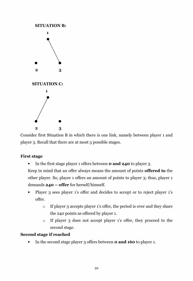
SITUATION B:
1
2 3
SITUATION C:
1
2 3
Consider first Situation B in which there is one link, namely between player 1 and
player 3. Recall that there are at most 3 possible stages.
First stage
• In the first stage player 1 offers between 0 and 240 to player 3.
Keep in mind that an offer always means the amount of points offered to the
other player. So, player 1 offers an amount of points to player 3; thus, player 1
demands 240 – offer for herself/himself.
• Player 3 sees player 1’s offer and decides to accept or to reject player 1’s
offer.
o If player 3 accepts player 1’s offer, the period is over and they share
the 240 points as offered by player 1.
o If player 3 does not accept player 1’s offer, they proceed to the
second stage.
Second stage if reached
• In the second stage player 3 offers between 0 and 160 to player 1.
92
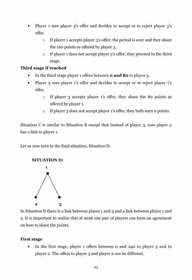
• Player 1 sees player 3’s offer and decides to accept or to reject player 3’s
offer.
o If player 1 accepts player 3’s offer, the period is over and they share
the 160 points as offered by player 3.
o If player 1 does not accept player 3’s offer, they proceed to the third
stage.
Third stage if reached
• In the third stage player 1 offers between 0 and 80 to player 3.
• Player 3 sees player 1’s offer and decides to accept or to reject player 1’s
offer.
o If player 3 accepts player 1’s offer, they share the 80 points as
offered by player 1.
o If player 3 does not accept player 1’s offer, they both earn 0 points.
Situation C is similar to Situation B except that instead of player 3, now player 2
has a link to player 1.
Let us now turn to the final situation, Situation D.
SITUATION D:
1
2 3
In Situation D there is a link between player 1 and 3 and a link between player 1 and
2. It is important to realize that at most one pair of players can form an agreement
on how to share the points.
First stage
• In the first stage, player 1 offers between 0 and 240 to player 3 and to
player 2. The offers to player 3 and player 2 can be different.
93
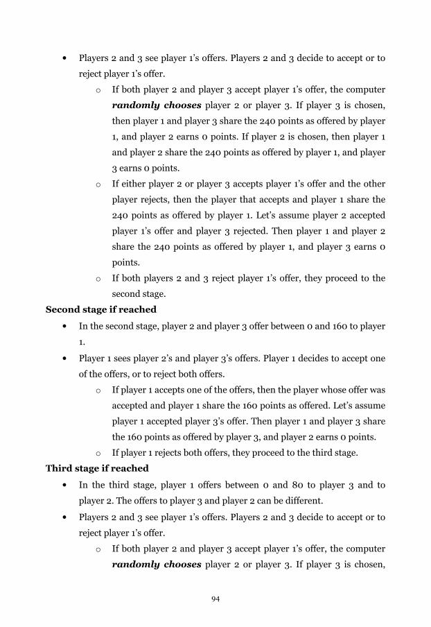
• Players 2 and 3 see player 1’s offers. Players 2 and 3 decide to accept or to
reject player 1’s offer.
o If both player 2 and player 3 accept player 1’s offer, the computer
randomly chooses player 2 or player 3. If player 3 is chosen,
then player 1 and player 3 share the 240 points as offered by player
1, and player 2 earns 0 points. If player 2 is chosen, then player 1
and player 2 share the 240 points as offered by player 1, and player
3 earns 0 points.
o If either player 2 or player 3 accepts player 1’s offer and the other
player rejects, then the player that accepts and player 1 share the
240 points as offered by player 1. Let’s assume player 2 accepted
player 1’s offer and player 3 rejected. Then player 1 and player 2
share the 240 points as offered by player 1, and player 3 earns 0
points.
o If both players 2 and 3 reject player 1’s offer, they proceed to the
second stage.
Second stage if reached
• In the second stage, player 2 and player 3 offer between 0 and 160 to player
1.
• Player 1 sees player 2’s and player 3’s offers. Player 1 decides to accept one
of the offers, or to reject both offers.
o If player 1 accepts one of the offers, then the player whose offer was
accepted and player 1 share the 160 points as offered. Let’s assume
player 1 accepted player 3’s offer. Then player 1 and player 3 share
the 160 points as offered by player 3, and player 2 earns 0 points.
o If player 1 rejects both offers, they proceed to the third stage.
Third stage if reached
• In the third stage, player 1 offers between 0 and 80 to player 3 and to
player 2. The offers to player 3 and player 2 can be different.
• Players 2 and 3 see player 1’s offers. Players 2 and 3 decide to accept or to
reject player 1’s offer.
o If both player 2 and player 3 accept player 1’s offer, the computer
randomly chooses player 2 or player 3. If player 3 is chosen,
94
then player 1 and player 3 share the 80 points as offered by player
1, and player 2 earns 0 points. If player 2 is chosen, then player 1
and player 2 share the 80 points as offered by player 1, and player
3 earns 0 points.
o If either player 2 or player 3 accepts player 1’s offer and the other
player rejects, then the player that accepts and player 1 share the
80 points as offered by player 1. Let’s assume player 2 accepted
player 1’s offer and player 3 rejected. Then player 1 and player 2
share the 80 points as offered by player 1, and player 3 earns 0
points.
o If both players 2 and 3 reject player 1’s offer, players 1, 2 and 3 earn
0 points.
To summarize:
You will be in a group of 3 persons. Each person will have her or his own number; 1,
2, or 3. Your number will be randomly determined at the beginning of the practice
period and it will stay the same throughout the experiment. Also, the composition
of your group will remain the same throughout the experiment. You will not know
who is in your group.
There will be 30 periods in the experiment. In every period there will be two parts.
First, you will decide with whom to link. Second, at most one pair of linked players
shares an amount of points. The important points of the experiment are the
following:
• A link is formed between two players if both of them offer a link to each
other.
• Player 2 and player 3 cannot form a link with each other.
• Only two players who have a link with each other can try to share a
certain amount of points among themselves.
• In the second part of the period, there are at most 3 stages. In the first
stage the amount to be shared is 240; in the second it is 160; in the
third it is 80.
• In the first stage player 1 can make on offer, in the second stage player
2 and/or player 3 can make an offer, and in the third stage player 1 can
95

make an offer. If there is no agreement in the third stage, everyone gets
0 points.
• At most one pair of players can reach an agreement in a period. When
there are two links and if both players 2 and 3 accepts player 1’s offer,
either player 2 or player 3 is chosen randomly by the computer to form
an agreement with player 1.
• In each period you will be informed about all the decisions made by
your group members. At the end of each period, you will be informed
about your and other players’ earnings.
• Your total earnings will be the sum of all points you earn over all
periods. For each point you earn in the experiment, you will get 0.5
Eurocents.
96

Chapter 4
The Stability of Exchange Networks∗∗∗∗
4.1. Introduction
An exchange situation can broadly be defined as a situation involving actors who
have the opportunity to collaborate for the benefits of all actors involved. While
exchange has been intensively studied in economics for more than a century (e.g.,
Coddington, 1968; Edgeworth, 1881; Young, 1975), exchange entered the fields of
social psychology and sociology only in the second half of the twentieth century.
Homans (1958: 606) introduced the idea that ‘social behavior is an exchange of
goods, material goods but also non-material ones, such as the symbols of approval
and prestige’. The conception of social behavior as exchange was also used by other
prominent social scientists in the same time period, such as Thibaut and Kelley
(1959) and Blau (1964). After these important works research on exchange as a
model of social behavior gained a prominent position in social psychology and
sociology.
Since Stolte and Emerson (1977) and Cook and Emerson’s (1978) seminal studies,
sociologists have focused on the effect of social structures on exchange outcomes.
The basic idea of this research is that social behavior is shaped by the social
relations in which it occurs, which are in return conditioned by the structures
within which they are embedded (Willer, 1999: xiii). Where social behavior is
conceived of as exchange, the social relation is dubbed an ‘exchange relation’ and
the structure is denoted an ‘exchange network’. If two persons have an exchange
relation, this means that both persons have the opportunity to exchange, but they
need not do so. If they do not have an exchange relation, they have no opportunity
to exchange. These opportunities and restrictions to exchange arise naturally in
many real-life situations. Three of the most common causes for the absence of an
exchange relation between two persons are natural barriers, non-matching
preferences, and the decreasing marginal utility of relations. Examples of barriers
∗ This chapter is based on Doğan, Van Assen, Van de Rijt, and Buskens (2009) published in Social Networks, 31, 118-125.
97

are not knowing each other, or not being able to contact or meet each other. Also,
two people might not have an exchange relation because one of them has nothing to
offer that is valuable enough to the other. Finally, if maintaining each tie is costly
and the marginal benefit of a relation decreases in the number of relations one
already has, it could be optimal to forego some relations.
In almost all sociological studies on exchange, both theoretical and empirical, the
social structure is the independent variable, i.e., what was studied was the effect of
the network structure on outcomes of persons in different network positions. These
studies show that network structure has a large impact on what actors earn in their
exchange relations (e.g., Willer, 1999; special issue Social Networks, June 1992;
special issue Rationality and Society, January 1997). The well-documented
tendency for exchange experiments with small sums of money to yield rather
egalitarian outcomes largely independent of experimental conditions (e.g., Roth,
1995) makes this result all the more pervasive. Since in different networks actors
obtain different exchange benefits, there is an incentive for actors to change the
network structure. Important questions are, therefore, how exchange networks
evolve in the first place, and which networks are stable or resistant to change. Note
that, although we attempt to answer these questions in the context of exchange
networks, these questions are relevant to any network in which benefit differences
between actors are substantial and depend on the network structure. Examples are
communication, knowledge, and friendship networks.
In our study the structure of the exchange network is the dependent variable. We
ask what structure can be expected to emerge if actors have the opportunity to
choose with whom to maintain exchange relations, as a function of tie costs. We
assume that tie costs are constant and both actors involved in a tie pay the tie costs.
Actors add and keep ties only if they are marginally beneficial. We investigate the
networks that are stable, and the networks that are efficient or egalitarian with
varying tie costs. We have two main results. First, sparse networks consisting of
only dyads and odd-sized cycles are both stable and egalitarian over a wide range of
tie costs. Second, we find that at low tie costs no even-sized network exists that is
both stable and efficient; we call this situation a ‘social dilemma’, i.e., actors end up
98
in networks where actors are unwilling to delete a tie to reach a network in which
all actors are better off.
We proceed as follows. In Section 4.2 we review the sociological exchange literature
and explain why we use Friedkin’s Expected Value Theory for determining
exchange benefits in exchange networks. We also outline the rules pertaining how
actors engage in exchange. In Section 4.3, we define network stability, efficiency,
and equality. In Section 4.4, we analyze the efficiency and equality of stable
networks as a function of tie costs. We present simulation results for networks up
to size 8 and prove three general theorems. These general theorems hold for
networks of any size and hold for all published theories of network exchange. We
conclude with a discussion in Section 4.5.
4.2. Theoretical Background
An exchange network is a set of actors and their exchange relations within this set.
Figure 4.1 depicts some examples of exchange networks. In these networks,
connected actors can exchange with each other. In sociological research on
exchange networks, two assumptions have been commonly made that we also make
in the present study (e.g., Willer, 1999; special issue Social Networks, June 1992;
special issue Rationality and Society, January 1997). First, an exchange relation is
represented as an opportunity to divide an exchange benefit of 24. Exchange occurs
if two connected actors can agree on a division. If they do not agree they obtain
nothing in that relation. Second, actors can only engage in one exchange, the so-
called one-exchange rule. Applied to the Line3 (see Figure 4.1), the one-exchange
rule implies that the central actor can exchange with one of the two peripheral
actors, but not with both.
99
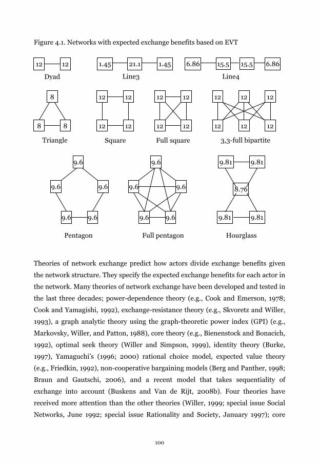
Figure 4.1. Networks with expected exchange benefits based on EVT
Theories of network exchange predict how actors divide exchange benefits given
the network structure. They specify the expected exchange benefits for each actor in
the network. Many theories of network exchange have been developed and tested in
the last three decades; power-dependence theory (e.g., Cook and Emerson, 1978;
Cook and Yamagishi, 1992), exchange-resistance theory (e.g., Skvoretz and Willer,
1993), a graph analytic theory using the graph-theoretic power index (GPI) (e.g.,
Markovsky, Willer, and Patton, 1988), core theory (e.g., Bienenstock and Bonacich,
1992), optimal seek theory (Willer and Simpson, 1999), identity theory (Burke,
1997), Yamaguchi’s (1996; 2000) rational choice model, expected value theory
(e.g., Friedkin, 1992), non-cooperative bargaining models (Berg and Panther, 1998;
Braun and Gautschi, 2006), and a recent model that takes sequentiality of
exchange into account (Buskens and Van de Rijt, 2008b). Four theories have
received more attention than the other theories (Willer, 1999; special issue Social
Networks, June 1992; special issue Rationality and Society, January 1997); core
8.76
9.81 9.81
9.81 9.81
12 12 1.45 21.1 1.45 6.86 15.5 15.5 6.86
8
8 8
12 12
12 12
12 12
12 12
12 12 12
12 12 12
9.6
9.6
9.6
9.6
9.6
9.6
9.6
9.6
9.6
9.6
Dyad Line3 Line4
Triangle Square Full square 3,3-full bipartite
Pentagon Full pentagon Hourglass
100
theory, power-dependence theory, expected value theory, and NET, which is a
combination of exchange-resistance, GPI, and optimal seek theories.
We use one of these exchange theories to determine what exchange benefits actors
obtain in a given network. Once exchange benefits are determined we can compare
the differences in benefits of actors across different networks. We can then
compute the exact effect of adding and deleting ties on actors’ exchange benefits.
Hence, an exchange theory is required that generates a unique point prediction for
the exchange benefits of each actor in each exchange network. Since core theory
and power-dependence theory do not provide unique point predictions they are not
suitable for our investigation. We did not select NET because there are several
different versions of the theory, and the most recent version of NET advocated by
its developers has not been computerized yet (Emanuelson 2005; Willer and
Emanuelson 2008). Consequently, we select the remaining theory: Friedkin’s
(1992, 1993, 1995) expected value theory (EVT). Although uniqueness and
existence for all networks is not proven, for every network up to 8 actors, the
algorithm of EVT generates a point prediction. Previous research suggests that
EVT, like other theories of network exchange, predict the outcomes of the exchange
networks that are realized in the lab with reasonable accuracy (e.g., Friedkin, 1995;
Van de Rijt and Van Assen, 2008).
After establishing the exchange benefits associated with each position in each
network by using EVT, differences in benefits of actors across networks can be
assessed. A number of studies have examined the effects of adding and deleting ties
to one actor on his expected benefits, his neighbors’ expected benefits, and the
overall power differences or variance in benefits in the network (Leik, 1991, 1992;
Van Assen and Van de Rijt, 2007; Willer and Willer, 2000). These studies examine
the effect of exogenous network changes, whereas we focus on endogenously stable
networks. That is, the actors in their studies are passive with respect to changing
ties, while the actors in our study actively consider deleting and adding ties to
maximize their expected benefits.
101
In our model, while the exact strategy space of the actors depends on the stability
concept employed, the unilateral deletion and bilateral addition of a tie is shared by
all stability concepts considered in this paper. An actor deletes a tie if the deletion
results in a network in which he obtains a larger payoff. A pair of actors adds a tie
between them if a network results in which at least one of them obtains a better
payoff and none of them fares worse. Actors thus only care about immediate
improvements in expected payoffs that are a direct consequence of their tie change.
They do not take potential future rewards into account that could result from
subsequent tie changes by other actors. They are myopic maximizers. Since both
actors in a tie pay the tie costs, establishing a link between two actors requires
mutual consent, whereas deletion of a tie is unilateral.
In this study it is assumed that equal tie costs are incurred for both actors involved
in a tie. Tie costs apply for each tie that an actor has. We vary the tie cost from 0 to
12 to analyze the impact of tie costs on the stable, efficient, and egalitarian
networks. Since the amount to be divided in an exchange is 24, there always exists
an actor who wants to delete a tie for tie costs higher than 12. Such costs need not
be considered. In this paper, we use the term expected benefits to refer to the
expected benefits from exchange minus the tie costs incurred.
Expected Value Theory (EVT)
Building upon the theory of social power proposed by French (1956), Friedkin
(1986) first suggested the idea of using expected values to predict the outcomes in a
power structure. Friedkin (1992; 1993) extended the idea of expected values to
analyze outcomes in an exchange network. Friedkin’s model predicts the
probability with which each maximal exchange pattern occurs, and the distribution
of outcomes in each one of these patterns. A maximal exchange pattern is maximal
in the sense that no further feasible transaction exists between the actors that have
not exchanged yet. For example, the Line4 (see Figure 4.1) has two maximal
exchange patterns: each peripheral actor exchanges with one of the central actors,
or the two central actors exchange with each other. Using an iterative algorithm,
each actor’s expected exchange benefits are calculated as the expected value of his
102
exchange benefits over all possible maximal exchange patterns (see Appendix 4A
for a detailed description of the EVT algorithm.)
Despite what the name suggests, EVT is not a theory based on actors rationally
maximizing their benefits. The algorithm generating the predictions assumes that
both actors’ claim of their share in their relation increases non-linearly in the
probability that each of them is excluded in any exchange. Three rules determine
the final allocation in the relation. Which rule is applied depends on the sum of
both actors’ claims and their claims relative to half of the exchange benefits to be
divided. See Friedkin (1995) for details of the EVT model. An inconvenience of the
EVT model is the analytical intractability of the algorithm because of the non-linear
function and the three rules embedded in it. Another characteristic of EVT is that
its predictions satisfy symmetry (i.e., automorphically equivalent positions get the
same payoff), however, invariance under scalar multiplication is violated (relative
share is affected if all resource pools are multiplied with the same constant). EVT
implies that the relative share of an actor decreases if the resource pool is
increased. See Van de Rijt and Van Assen (2008) for an overview of properties of
EVT and other theories of network exchange.
Figure 4.1 shows expected exchange benefits predicted by EVT for several
networks. For example, in the Line3, it is expected that the peripheral actor who
exchanges with the central actor receives 2.9 out of 24, while the central actor
obtains 21.1. Because peripheral actors are only expected to exchange half of the
time, their expected benefit is 1.45.
4.3. Definitions of Stability, Equality, and Efficiency
We borrow our definitions of what constitutes a stable network from a rapidly
growing literature on network formation in economics (e.g., Demange and
Wooders, 2005; Dutta and Jackson, 2003; Goyal, 2007). Some networks
considered in this literature are similar to exchange networks. By doing so, we
bring together research on network exchange in sociology and research on network
formation in economics.
103
Stability
Jackson and Wolinsky (1996) introduced the pairwise stability concept. In his
survey on network formation Jackson (2003) argues that pairwise stability might
be considered a necessary condition for network stability. It is the weakest notion
of stability that allows for tie formation while providing narrow predictions about
the set of stable networks. An exchange network is pairwise stable if (i) adding a
currently absent tie is costly to at least one of the two actors involved or leaves both
actors equally well off, (ii) removing a present tie does not benefit either of the two
actors it currently connects.
As an example of how to use the notion of pairwise stability, consider an 8-actor
network where one actor is connected to three other actors, but not to the
remaining four actors. This can be denoted by an ‘adjacency row’ 1110000, where
the 1’s indicate the three existing relations and the 0’s the four absent relations.
Then, with regard to the focal actor, pairwise stability holds if no single change
from 1 to 0 (the deletion of one tie) increases this actor’s expected benefits, and if
no single change from 0 to 1 (the addition of one tie) increases the expected
benefits of the focal actor while not decreasing the expected benefits of the other
actor in this relation. A network is pairwise stable if the conditions above hold for
each actor in the network.
In our analysis we also use two stronger stability concepts that are refinements of
pairwise stability: pairwise Nash and unilateral stability. Pairwise Nash is a
refinement of pairwise stability, and unilateral stability is a refinement of pairwise
Nash. We use these two additional concepts for two reasons. First, we want to
examine whether our results are robust against alternative stability concepts.
Second, we are able to prove two general theorems using pairwise Nash, which we
cannot by using pairwise stability.
A network is strongly pairwise stable (Gilles and Sarangi, 2004) or pairwise Nash
(Calvó-Armengol and İlkılıç, 2005) if (i) adding a presently absent tie is costly to at
least one of the two actors or leaves both actors equally well off; and (ii) removing a
104
subset of an actor’s present ties does not benefit this actor. Note that condition (i)
of pairwise Nash is identical to condition (i) of pairwise stability. The difference
between pairwise stability and pairwise Nash is that pairwise Nash allows for
simultaneous deletions of ties. Continuing our previous example, consider again
the 8-actor network with adjacency row equal to 1110000 for the focal actor.
Pairwise Nash holds for this actor if each change of one 0 to 1 does not increase his
expected benefits and the other actor is not worse off, and each change of a subset
of 1s to 0s does not increase the focal actor’s expected benefits. A network is
pairwise Nash if this condition holds for each actor in the network.
A network is unilaterally stable (Buskens and Van de Rijt, 2008a; Van de Rijt and
Buskens, 2007) if no actor can profitably reconfigure his ties without objection by
his new contacts. Different from pairwise stability, unilateral stability allows for
simultaneous addition and deletion of ties such that actors can replace one tie with
another as long as the addition of each new tie does not make the actor in the new
tie worse off33. In our example, unilateral stability holds for the focal actor if no
adjacency row other than 1110000 simultaneously (i) increases this actor’s
expected benefits, and (ii) makes no actor who is connected to the focal actor in the
new network but disconnected in the old network worse off. Only the actors newly
connected have to agree, because only for creating new ties mutual consent is
required. A network is unilaterally stable if this condition holds for each actor in
the network.
Egalitarian Networks
Networks are defined as egalitarian if all actors in the network obtain the same
expected benefits in which the subtraction of the tie costs is included. Some
examples of egalitarian networks are complete networks, cycles, and even-sized
33 If a network is unilaterally stable, then it is also pairwise stable, but the opposite is not
true. Hence it is possible that a network is pairwise stable at some cost level but not
unilaterally stable; even if it is not profitable to add a tie, or delete ties, an actor might
profitably reconfigure his network by adding more than one tie, or replacing some of his ties.
105
networks consisting of only dyads. We will categorize stable networks that are
egalitarian.
Efficiency
With the introduction of tie costs inefficient pairwise stable networks might arise.
We distinguish two forms of efficiency. First, a network is socially efficient if, given
tie costs, there is no other network in which the sum of the expected benefits is
larger than in this network. Second, a network is Pareto efficient if there exists no
other network in which no actor earns less and at least one actor earns more than
in the given network. We will investigate if there are tie cost levels for which no
pairwise stable network of a given size is Pareto efficient. If such tie cost levels
exist, we say that there is a tension between efficiency and stability and say that a
social dilemma exists. It is easy to see that social efficiency implies Pareto
efficiency.
4.4. Results
Friedkin’s EVT is a system of many assumptions and equations that makes a formal
analysis very difficult. However, we prove some general results on stability that
concern networks of any size and do not depend on the use of EVT as a prediction
method of exchange benefits. In addition, to get more insight into the properties of
stable networks, we analyze a subset of exchange networks; all 13,597 non-
isomorphic exchange networks of size 2 through 8. We first present simulation
results for these small networks obtained with EVT, and then prove our general
results.
Simulation Results
For all exchange networks of size 2 through 8, we computed at what tie cost levels
each exchange network is pairwise stable, pairwise Nash, or unilaterally stable. In
order to find these cost levels, we calculated for each network, the highest cost level
h for which some pair of actors still wants to add a tie. In addition, we calculated
106

the lowest cost level l for which some actor still wants to remove one or more ties
(depending on the stability concept). Whenever the resulting interval [h, l] is not
empty, the network is stable for the cost levels in this interval. The reason is that for
these cost levels, tie costs are too high to add ties and too low to remove ties.
Because we also need to check for simultaneous removal and addition of ties to
establish unilateral stability, some more conditions need to be checked for
unilateral stability. The details of this procedure can be obtained from the
authors.34
A first general observation is that there are rather few networks (at least for not too
small network size) that are stable within some tie cost range, and that the
proportion of stable networks decreases quickly with network size. If network size
is 6, 17 out of 156 networks are pairwise stable of which 16 are pairwise Nash and 13
are unilaterally stable. This is about 10% of the total number of networks of size 6.
When network size is 7, 40 out of 1,044 networks are pairwise stable, of which 34
are pairwise Nash and 30 unilaterally stable. Here the proportion of stable
networks is around three percent. Finally, for network size 8, 105 out of 12,346
networks (less than 1%) are pairwise stable of which 93 are pairwise Nash and 72
are unilaterally stable.
Table 4.1 provides detailed information for a subset of stable networks, namely
those that are pairwise stable over a tie cost range spanning at least 1 exchange
point (out of 24). We use the names triangle, square, pentagon, hexagon, etc. for
cycles of 3, 4, 5, 6 etc. actors. The word “full” is added if we refer to the complete
network with the same number of actors (see also Figure 4.1). Table 4.1 reports
lower and upper bounds on the tie cost intervals for which the networks are stable.
The lower bound for pairwise Nash is not reported because it coincides with the
lower bound for pairwise stability. The reason is that they both refer to the highest
cost level for which some pair of actors still wants to add a tie. The table also
reports the density, tie costs for which the network is egalitarian, and tie costs for
34 All calculations were programmed in Borland Delphi. The source code is available from
the authors upon request.
107

Tab
le 4
.1 P
airw
ise
stab
le n
etw
orks
th
at a
re s
tabl
e in
a t
ie c
ost
ran
ge la
rger
th
an o
ne3
5
Net
wor
k
Siz
e
Low
er
bou
nd
for
pai
rwis
e
stab
ilit
y
Up
per
bou
nd
for
pai
rwis
e
stab
ilit
y
Up
per
bou
nd
for
pai
rwis
e
Nas
h
Low
er
bou
nd
for
un
ilat
eral
stab
ilit
y
Up
per
bou
nd
for
un
ilat
eral
stab
ilit
y D
ensi
ty
Tie
cos
ts f
or
wh
ich
egal
itar
ian
Tie
cos
ts f
or
wh
ich
pai
rwis
e
stab
le &
Par
eto
effi
cien
t
dya
d
2 –
∞
12
12
–∞
12
1
alw
ays
≤12
dya
d, i
sola
te
3
1.4
49
12
12
1.
44
9
12
0.3
33
12
1.4
49
-12
Tri
angl
e –
∞
6.5
51
4
–∞
4
1
alw
ays
<4
35 T
he
nu
mbe
r of
net
wor
ks t
hat
are
pai
rwis
e st
able
in
som
e co
st r
ange
sm
alle
r th
an 1
an
d h
ence
not
in
clu
ded
in
th
e ta
ble
for
size
2 t
o 8
are
resp
ecti
vely
, 0, 0
, 0, 2
, 7, 2
8, a
nd
88
. Th
ere
is o
ne
oth
er n
etw
ork
for
size
6 t
hat
is e
gali
tari
an a
nd
sta
ble
in a
sm
all r
ange
an
d o
ne
that
is e
gali
tari
an
but
not
sta
ble.
Th
ere
is a
lso
one
oth
er e
gali
tari
an n
etw
ork
wit
h 7
act
ors
that
is s
tabl
e in
a s
mal
l ran
ge. T
her
e ar
e 7
oth
er n
etw
orks
of
size
8 t
hat
are
egal
itar
ian
fro
m w
hic
h 6
fu
lfil
l all
sta
bili
ty c
rite
rion
s fo
r a
smal
l ran
ge. T
he
rem
ain
ing
net
wor
k is
un
stab
le.
Th
ere
are
oth
er n
etw
orks
th
at a
re p
airw
ise
stab
le a
nd
Par
eto
effi
cien
t es
pec
iall
y fo
r si
zes
equ
al t
o 5
and
7 f
or s
mal
l co
st r
ange
s. E
xam
ple
s ar
e th
e
hou
rgla
ss a
nd
th
e h
ourg
lass
+ d
yad
, wh
ich
are
bot
h p
airw
ise
stab
le a
nd
Par
eto
effi
cien
t fo
r co
st =
1.
All
th
ese
oth
er n
etw
orks
are
non
-ega
lita
rian
and
hav
e a
subs
et o
f act
ors
wh
o ar
e re
lati
vely
wel
l off
.
A c
omp
lete
ove
rvie
w o
f th
e ra
nge
s fo
r w
hic
h n
etw
orks
of
size
s 2
to 8
are
sta
ble
is a
vail
able
fro
m t
he
auth
ors.
108
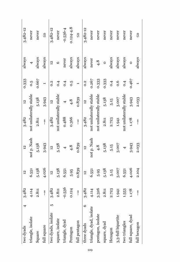
two
dya
ds
4
3.
48
2 12
12
3.
48
2 12
0
.333
al
way
s 3.
48
2-12
tria
ngl
e, is
olat
e 4
.114
6
.551
n
ot p
. Nas
h
not
un
ilat
eral
ly s
tabl
e 0
.5
4
nev
er
Squ
are
2.8
11
5.13
8
5.13
8
2.8
11
5.13
8
0.6
67
alw
ays
nev
er
full
squ
are
–∞
4
.026
3.
94
3 –
∞
3.9
43
1 al
way
s ≤
0
two
dya
ds,
isol
ate
5 3.
48
2 12
12
3.
48
2 12
0
.2
12
3.4
82-
12
squ
are,
isol
ate
2.8
11
5.13
8
5.13
8
not
un
ilat
eral
ly s
tabl
e 0
.4
6
nev
er
tria
ngl
e, d
yad
-0
.536
6
.551
4
0
.48
8
4
0.4
n
ever
-0
.536
-4
Pen
tago
n
0.1
24
5.9
5 4
.8
0.3
66
4
.8
0.5
al
way
s 0
.124
-4.8
full
pen
tago
n
–∞
0
.839
0
.839
–
∞
0.8
39
1 al
way
s ≤
0
thre
e d
yad
s
6
3.4
82
12
12
3.4
82
12
0.2
al
way
s 3.
48
2-12
tria
ngl
e, d
yad
, iso
late
4
.114
6
.551
n
ot p
. Nas
h
not
un
ilat
eral
ly s
tabl
e 0
.26
7 n
ever
n
ever
pen
tago
n, i
sola
te
3.32
6
5.9
5 4
.8
not
un
ilat
eral
ly s
tabl
e 0
.333
4
.8
nev
er
squ
are,
dya
d
2.8
11
5.13
8
5.13
8
2.8
11
5.13
8
0.3
33
0
nev
er
Hex
agon
2.
723
5.15
5.
15
2.72
3 5.
15
0.4
al
way
s n
ever
3,3-
full
bip
arti
te
1.9
41
3.0
07
3.0
07
1.9
41
3.0
07
0.6
al
way
s n
ever
two
tria
ngl
es
1.55
3 6
.551
4
n
ot u
nil
ater
ally
sta
ble
0.4
al
way
s n
ever
full
squ
are,
dya
d
1.17
8
4.0
26
3.9
43
1.17
8
3.9
43
0.4
67
0
nev
er
full
hex
agon
–
∞
2.10
4
2.0
33
–∞
2.
033
1
alw
ays
≤0
109
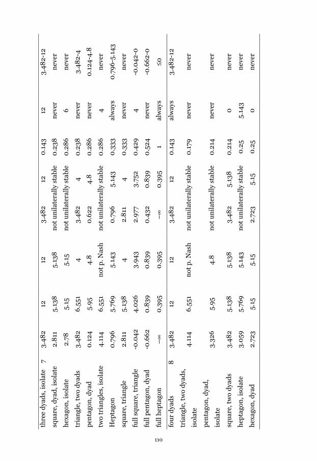
thre
e d
yad
s, is
olat
e
7
3.4
82
12
12
3.4
82
12
0.1
43
12
3.4
82-
12
squ
are,
dya
d, i
sola
te
2.8
11
5.13
8
5.13
8
not
un
ilat
eral
ly s
tabl
e 0
.238
n
ever
n
ever
hex
agon
, iso
late
2.
78
5.15
5.
15
not
un
ilat
eral
ly s
tabl
e 0
.28
6
6
nev
er
tria
ngl
e, t
wo
dya
ds
3.4
82
6.5
51
4
3.4
82
4
0.2
38
nev
er
3.4
82-
4
pen
tago
n, d
yad
0
.124
5.
95
4.8
0
.622
4
.8
0.2
86
n
ever
0
.124
-4.8
two
tria
ngl
es, i
sola
te
4.1
14
6.5
51
not
p. N
ash
n
ot u
nil
ater
ally
sta
ble
0.2
86
4
n
ever
Hep
tago
n
0.7
96
5.
769
5.
143
0.7
96
5.
143
0.3
33
alw
ays
0.7
96
-5.1
43
squ
are,
tri
angl
e 2.
811
5.
138
4
2.
811
4
0
.333
n
ever
n
ever
full
squ
are,
tri
angl
e -0
.04
2 4
.026
3.
94
3 2.
977
3.
752
0.4
29
4
-0.0
42-
0
full
pen
tago
n, d
yad
-0
.66
2 0
.839
0
.839
0
.432
0
.839
0
.524
n
ever
-0
.66
2-0
full
hep
tago
n
–∞
0
.39
5 0
.39
5 –
∞
0.3
95
1 al
way
s ≤
0
fou
r d
yad
s
8
3.4
82
12
12
3.4
82
12
0.1
43
alw
ays
3.4
82-
12
tria
ngl
e, t
wo
dya
ds,
isol
ate
4.1
14
6.5
51
not
p. N
ash
n
ot u
nil
ater
ally
sta
ble
0.1
79
nev
er
nev
er
pen
tago
n, d
yad
,
isol
ate
3.32
6
5.9
5 4
.8
not
un
ilat
eral
ly s
tabl
e 0
.214
n
ever
n
ever
squ
are,
tw
o d
yad
s 3.
48
2 5.
138
5.
138
3.
48
2 5.
138
0
.214
0
n
ever
hep
tago
n, i
sola
te
3.0
59
5.76
9
5.14
3 n
ot u
nil
ater
ally
sta
ble
0.2
5 5.
143
nev
er
hex
agon
, dya
d
2.72
3 5.
15
5.15
2.
723
5.15
0
.25
0
nev
er
110
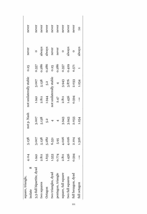
squ
are,
tri
angl
e,
isol
ate
8
4.1
14
5.13
8
not
p. N
ash
n
ot u
nil
ater
ally
sta
ble
0.2
5 n
ever
n
ever
3,3-
full
bip
arti
te, d
yad
1.
94
1 3.
00
7 3.
00
7 1.
94
1 3.
00
7 0
.357
0
n
ever
two
squ
ares
2.
811
5.
138
5.
138
2.
811
5.
138
0
.28
6
alw
ays
nev
er
Oct
agon
1.
635
5.
282
5.2
1.9
44
5.
2 0
.28
6
alw
ays
nev
er
two
tria
ngl
es, d
yad
1.
553
6.5
51
4
not
un
ilat
eral
ly s
tabl
e 0
.25
nev
er
nev
er
pen
tago
n, t
rian
gle
0.7
74
5.9
5 4
2.
47
4
0.2
86
n
ever
n
ever
squ
are,
fu
ll s
quar
e 2.
811
4
.026
3.
94
3 2.
811
3.
94
3 0
.357
0
n
ever
two
full
squ
ares
1.
456
4
.026
3.
94
3 1.
456
3.
876
0
.429
al
way
s n
ever
full
hex
agon
, dya
d
0.5
94
2.
104
2.
033
0
.59
4
2.0
33
0.5
71
0
nev
er
full
oct
agon
–
∞
1.32
6
1.25
4
–∞
1.
254
1
alw
ays
≤0
111
which the network is both pairwise stable and Pareto efficient. Stable networks in
Table 4.1 consist of either one component or of multiple disconnected components
in which everybody has an automorphically equivalent position and therefore
expects the same benefits. Between components there can be differences in
expected benefits. Note that if all components are identical, stable networks are
egalitarian irrespective of the tie costs.
Social efficiency is not included in the table because for positive tie costs the only
socially efficient networks that exist are the dyads, possibly in combination with
one isolate if the number of actors is odd. We call the unconnected dyads and at
most one isolate M(inimal) networks. Given nonzero tie costs M networks are the
unique socially efficient networks. In M networks the maximum number of
exchanges is realized with a minimal number of ties. Total exchange benefits can
never be larger and costs are minimized in M networks. In Table 4.1 we see that all
socially efficient M networks are stable if tie costs are large enough, larger than
3.48 in the case of EVT. For even-sized networks, these networks are also
egalitarian, and Pareto efficient. For odd-sized networks, there is some inequality
in these networks because one actor obtains nothing.
The density of stable networks in general decreases with tie costs, although not
monotonically. As an example, consider the pairwise stable networks of size 4. All
pairwise stable networks of size 4 are listed in Table 4.1. For tie costs in the interval
[0, 4.026], the complete network with density 1 is pairwise stable. The square (4-
cycle) with density 2/3 is pairwise stable for tie costs in [2.811, 5.138]. The M
network (2 dyads) with density 1/3 is pairwise stable when tie costs are in [3.482,
12]. A triangle and an isolate, with density 1/2, is pairwise stable for tie costs in
[4.114, 6.551]. Interestingly, the often investigated Line4 network is not stable at
any tie cost; for tie costs larger than 3.482 the actors with two ties prefer to delete
their connection in order to form a dyad, and for tie costs smaller than 5.138 the
two peripherals prefer to be connected to each other. Hence, our analysis suggests
that in real-life exchange settings that resemble the point of departure of our
analysis, the Line4 network will not occur often.
112
Because stable networks at low tie costs have a higher density than the socially
efficient M networks, a social dilemma situation might exist. Indeed, if tie costs are
smaller than 3.48 the even-sized M network is not stable (see also Theorem 2
below) but Pareto dominates the stable networks for such tie costs. Hence EVT
predicts social dilemma situations for tie costs smaller than 3.48 in even-sized
exchange networks of size 4, 6, 8; the networks will evolve into stable networks that
are ‘overconnected’ and Pareto dominated by the M networks. In odd-sized
networks, there exist other Pareto efficient stable networks in addition to the M
network because all actors gain more than the isolate in the M network.
Although most networks listed in Table 4.1 as well as the other stable networks are
not egalitarian, differences in exchange benefits across actors are mostly not large.
First, no pairwise stable network is a so-called ‘strong power’ network (Willer,
1999: 109-111), i.e., there is no network up to size 8 with a minority of actors
earning almost all points in their exchange relations. The largest benefit differences
arise in odd-sized M networks. Within components some actors might earn a bit
more than others, the hourglass network with five actors (see Figure 4.1) is one
example, but if power difference becomes too large within components, there are
always actors in these components who do seek other exchange relations, rendering
the network unstable.
Analytic Results
The analysis of networks up to size 8 demonstrates that M networks are important:
they are efficient, stable for a large tie cost interval, and egalitarian if the network
size is even. Here we show some general results on the efficiency (Theorem 1) and
stability (Theorem 2 and 3) of M networks of any size. Throughout the remainder
of the section, the only assumptions made about the distribution of exchange
benefits with no side payments are36 (i) if two actors can exchange with one
36 The assumptions are related only to the distribution of exchange benefits. Hence the
results apply to any exchange distribution mechanism given that (i) the networks are
undirected under the 1-exchange rule, (ii) there is mutual consent for tie addition, (iii) tie
113
another and do not exchange with third parties then they will exchange with one
another, and (ii) if they both have only one exchange relation they divide exchange
benefits in that relation equally. With the exception of core theory – which leaves
exchange divisions in isolated dyads unspecified – all exchange theories that have
been proposed in the sociological literature satisfy these requirements.
As we have already argued in the previous subsection, M networks are socially
efficient networks and, therefore, they are also Pareto efficient as is summarized in
the first theorem.
Theorem 1: An M network is socially efficient (and therefore also Pareto efficient)
for any tie cost c in the closed interval [0, 12].
Proof of theorem 1: Total benefits are maximal because the maximum number of
exchanges, n/2 (rounded down if n is odd), is always carried out. Any additional tie
reduces the total profit by 2c. Also, the marginal benefit of each tie in the M
network is 24, which is the highest possible marginal benefit a tie can have. For c in
[0, 12], the increase in net total benefit from each of these ties is nonnegative.
Q.E.D.
In particular, M networks are the only socially efficient networks for tie costs in the
interval (0, 12). There are other socially efficient networks if tie costs are equal to 0,
because in that case any network that guarantees the maximal number of
exchanges is socially efficient. There are also other Pareto efficient networks. For
even-sized networks, these Pareto efficient networks are non-egalitarian. By
definition an M network has the minimum number of ties with the maximum
number of exchanges. Hence, any Pareto efficient network other than the M
network has more ties than the M network. If another Pareto efficient network is
also egalitarian, then the M network Pareto dominates it for any tie cost larger than
zero, which is a contradiction. None of the other Pareto efficient even-sized stable
networks are included in Table 4.1, since these networks are stable only for narrow
tie cost ranges. For odd-sized networks, many Pareto-efficient stable networks
deletion is unilateral, and (iv) equal tie costs are incurred for both parties in the tie.
114
exist. One of these networks is the cycle with all actors involved, which is
egalitarian and stable over a wide range of tie costs.
M networks are unilaterally stable (and hence pairwise Nash, and pairwise stable)
for high tie costs. For pairwise Nash and pairwise stability, this result can be
generalized to networks of any size and any exchange theory, as Theorem 2 shows.
Consider a value d = max(e – 12, min(f – 12, g)), where e is the exchange benefit of
a central actor in the Line4, f the exchange benefit of the central actor in the Line3,
and g the exchange benefit of the peripheral actor in the Line3. For example, d =
3.48 for EVT, since e = 15.48, f = 21.1, and g = 1.45.
Theorem 2: An M network of any size is pairwise Nash (and therefore also
pairwise stable) for tie costs c in (d, 12).
Proof of Theorem 2: Because everyone with a tie obtains benefits from the
exchange equal to 12 in an M network, no one wants to remove a tie as long as the
tie costs are below 12. Since actors can only add one tie, there are only two possible
additions. First, if two dyads connect with each other the connecting actors see
their exchange benefits raise to e. Thus, to make this change unprofitable, tie costs
should exceed the marginal benefits of these actors, which equal e – 12. In odd-
sized networks the isolate can try to connect to a dyad, raising his partner’s
expected benefits to f, obtaining g himself. For this tie addition to be unprofitable,
tie costs should exceed the lowest marginal benefit across the two actors, which is
min(f – 12, g). Therefore, pairwise Nash stability is established for the interval (d,
12). Q.E.D.
Table 4.1 suggests that given EVT benefits, the M network is the only pairwise
stable network at tie costs larger than 6.55. Networks other than M networks that
are pairwise stable at, e.g., c = 6.5, consist of combinations of triangles, dyads, and
at most one isolate. We were unable to prove that M networks are the only pairwise
stable networks for any tie costs c in (6.55, 12) using EVT. Nonetheless, we can
prove that with tie costs c in (6, 12), the only pairwise Nash and unilaterally stable
networks are M networks regardless of the theory used. Note that triangles are not
115
pairwise Nash for c > 4 since one actor can improve his payoffs with 2c – 8 by
deleting two links at the same time.
Theorem 3: The only pairwise Nash (and unilaterally stable) networks with c in
(6, 12) are M networks.
Proof of Theorem 3: The networks with fewer ties than M networks are not stable
since tie addition is profitable for two isolates. Hence, it suffices to show that in any
network with more ties than an M network with c in (6, 12) at least one actor wants
to delete at least one of his ties. Such a network has at least one actor with two ties.
Let’s first assume everyone has more than one tie. Then everyone pays more than
12 for the ties. However, not everybody can earn more than 12. Thus, someone has
negative net earnings and is better off deleting all ties. Hence, there should be at
least one actor with one tie who has a neighbor with at least two ties (otherwise we
have the M network). Let us label the actor with one tie as A, A’s neighbor with at
least two ties as B, and one of B’s neighbors other than A as C. Actor A should have
at least an expected benefit c from exchange, otherwise he would remove the tie.
Actor B should have at least 12 + c as exchange benefit from his two ties, otherwise
he would remove all his ties except with A, and get an exchange benefit of 12. But
actor B can earn at most 24 − c from his exchange with A which is less than 12 + c
for c in (6, 12). So actor B should earn more than 24 − c in at least one of his other
exchanges, and without loss of generality this neighbor is C. However, now actor C
earns less than c from his exchange with B, and hence actor C prefers to delete the
tie. Q.E.D.
4.5. Discussion
Research on network exchange in sociology has focused on the effect of the social
structure on outcomes of exchange. In almost all of this research, the exchange
network has been exogenous and the independent variable. The main result of this
research is that network structure has a large impact on what actors earn in their
exchange relations. Because positions in different networks obtain different
benefits, there exist incentives for actors to change the network. Subsequently, the
questions of how these networks evolve, and which networks are stable arise. In the
116
current article we study what the network structure looks like if actors have the
opportunity to choose with whom they have an exchange relation, that is, the
network structure is our dependent variable.
We investigate the networks that are stable, the networks that are efficient or
egalitarian with varying tie costs, and the occurrence of social dilemmas. We
employed the assumptions mostly used in the sociological literature on exchange
networks, including the one-exchange rule and that the value of each exchange
relation is the same. Additionally, we assume that actors delete and add ties in
order to maximize their expected benefits; for adding ties mutual consent is
needed, whereas tie deletion is unilateral. Ties are costly and the costs are the same
for both actors in the tie. To assess the stability of exchange networks we employ
three stability concepts from the economic literature on networks: pairwise
stability, pairwise Nash, and unilateral stability. In addition, social efficiency and
Pareto efficiency are used as efficiency measures, and the networks are considered
egalitarian if all actors in the network expect the same benefits. To calculate the
actors’ expected benefits we use Friedkin’s Expected Value Theory. First, we
investigate all networks up to size 8. Then we prove three general results.
Few networks are stable over a wide range of tie costs, and all of them can be
divided into two types: M networks consisting of only dyads and at most one
isolate, and cycles with an odd number of actors. Even-sized M networks and odd
cycles are egalitarian. As we have shown, M networks of any size are the only
socially efficient networks for any tie costs but they are only stable starting from
intermediate cost levels. Hence, any stable network is socially inefficient at low tie
costs. Finally, we observe social dilemmas at low tie costs in even-sized networks;
that is, none of the (socially inefficient) stable networks are Pareto efficient. Using
pairwise Nash or unilateral stability does not change any of these results.
A remarkable result is that almost all egalitarian networks up to size 8 are stable at
some tie costs. Although actors in our model maximize their own expected benefits
that do not include equality preferences, they can be “satisfied” in egalitarian
networks. Nonetheless, many non-egalitarian networks are stable as well. Thus, it
117
is an interesting empirical question whether exchange networks evolve into non-
egalitarian networks in real world settings. To what extent actors’ preferences for
equality [as in Fehr and Schmidt (1999)] do affect the stability of networks, and
whether these preferences are observed in the evolution of (exchange) networks
remains to be examined.
Although there exist stable networks that are also efficient at some tie costs, most
stable networks are not efficient. Hence, tensions between stability and efficiency
arise over a wide range of tie costs. This tension is strongest in even-sized networks
at low tie costs where social dilemmas occur, because at such tie costs no stable
network is Pareto efficient. It is an interesting empirical question whether actors
resist the immediate temptation and end up in the both socially and Pareto efficient
but not stable M network. Preferences for efficiency can be incorporated in the
actors’ utility function as in Charness and Rabin (2002), and the effect of efficiency
and equality preferences on the evolution and stability of networks can thus be
examined.
The results of our study can be compared to those of Bonacich (2001), and Van de
Rijt and Buskens (forthcoming) who studied the dynamics of sociological exchange
networks. Bonacich (2001) simulated exchange network evolution and found that,
in equilibrium, differences in benefits were small. One important difference
between our analysis and Bonacich’s analysis is that in his simulation the actors are
assumed to be myopic satisficers such that they change the network if their
earnings drop below a certain level. In our study, however, the actors are assumed
to be myopic maximizers such that they change the network as long as marginal
benefits outweigh marginal tie costs. Another difference is that instead of adding or
deleting ties, Bonacich’ actors move to another cell on a checkerboard, where they
can exchange with actors in adjacent squares. Interestingly, despite these different
assumptions, he also arrives at the conclusion that in equilibrium networks are
egalitarian. Bonacich (2004) provides some intuitions for how this approach can be
extended to more general structures. Van de Rijt and Buskens (forthcoming)
analyzed the stability of exchange networks employing the same stability concepts,
but using another exchange theory, and without focusing on efficiency and equality.
118
Our stability results are very similar to the ones reported in their paper, and
confirm the robustness of the dynamics results across exchange theories.
The focus of the present article is on the possible path ends of the evolution of
exchange networks, i.e., the stable networks. Consequently, a natural extension is
investigating how to get to these possible endpoints, i.e., the evolution of the
network. The probability of reaching each stable network could also be
investigated. Factors that could determine these probabilities are the initial
network configuration, tie costs, and preferences for equality and efficiency. It
might also be that stable networks differ in their robustness to the errors of actors.
In some stable networks one error might be enough to move to another stable
network, whereas other stable networks might be stable after one or more
accidental errors. Such issues remain to be investigated both in the laboratory, and
by theory or simulation.
In our analysis we assume that actors are myopic; they only take their immediate
benefits into account but not the consequences of their behavior on future benefits.
The justification of this assumption is that not only it makes the analysis more
tractable, but also that actor behavior in the laboratory seems to be rather myopic
as well. Most actors are found to think two, or at most three steps ahead in many
different experimental games (Camerer 2003, Ch. 5). Nevertheless, in their book on
network formation Dutta and Jackson (2003:13) argue that allowing for farsighted
actors in models of network evolution is “perhaps the most important (and possibly
the hardest) issue regarding modeling the formation of networks”. Actors taking
the future into account are likely to affect the evolution and stability of exchange
networks. To mention two examples, taking the future into account gives
opportunities to solve social dilemmas and the problems of inefficiency of stable
networks as described above. An even-sized M network that is efficient but not
stable can be sustained as equilibrium if the actors are rational and the ‘network
evolution game’ is indefinitely repeated. Similarly, an odd-sized M network that is
efficient but neither stable at low tie costs nor egalitarian can be sustained as
equilibrium if the shadow of the future is sufficiently long, and if the actors
119
coordinate on alternating the excluded actor. Alternating the excluded actor
ensures that both efficiency and equality are satisfied.
The implications of the current study extend to other social networks among which
are communication, knowledge, and friendship networks. In these networks similar
questions of stability are of interest such as whether only few networks are stable,
and whether stable networks tend to be egalitarian. As Jackson and Wolinsky
(1996) showed with a theorem in their seminal paper, there exist a tension between
stability and efficiency in different economic and social network contexts. Thus,
analyzing whether actors form socially inefficient but stable networks that
correspond to social dilemma situations is particularly appealing. For example,
Buskens and Van de Rijt (2008a) show that efficiency, stability, and equal divisions
of outcomes can also go hand in hand even in competitive network formation
settings in which everybody strives for a central network position. Considering the
importance of network studies in aforementioned fields, more of such analyses are
to be expected.
120
Appendix 4A. Expected Value Theory
Building upon the theory of social power proposed by French (1956), Friedkin
(1986) first suggested the idea of using expected values to predict the outcomes in a
power structure. Friedkin (1992; 1993) extended the idea of expected values to
analyze outcomes in an exchange network. In this expected value model of social
exchange, Friedkin defines R-networks and their probabilities, and a method to
calculate the expected value of a certain position in a certain R-network. An R-
network is defined as a subset of exchange relations. An R-network is assumed to
be maximal in the sense that no further feasible transaction exists. For example,
consider the Line4 that has two R-networks; R1 = {{A-B}, {C-D}} and R2 = {{B-C}}.
Friedkin (1995) introduced a function of offers, fij, made by actor i to actor j. If 24
points are divided in the exchange, fij amounts to
124 23 id
f ij−= − (1)
Friedkin claims that the function fij is built on the theory of Cook and Emerson
(1978) where actors lower their offers when their offers are not accepted. He
introduces the dependency of actor i on j, di, which, under a 1-exchange rule, is
simply the probability that actor i is not involved in an exchange. The following
three assumptions deal with what happens to the outcomes or values obtained by
the actors in the relation when the personal claims 24 – fij and 24 – fji do not add
up to the amount of available resources, 24. The first assumption says that when
the actors’ personal claims sum up to more than the available resources, they get
the average of the difference between their claims plus available resources. To
illustrate the idea: when fij is 4 and fji is 8, i’s and j’s personal claims are 20 and 16
respectively. Hence, the first assumption states that player i will obtain (24+20–
16)/2 which is 14 and j will obtain (24+16-20)/2 which is 10. The second
assumption says that if both actors claim less than one-half of the resources, they
split the resources equally. The third assumption says that if one actor claims less
than one-half and the other claims one-half or more and the sum of the two claims
is less than the available resources, the unclaimed portion is allocated to the one
who asks for less.
121

The iterative algorithm of the 1995 version of EVT subsequently updates exchange
outcomes, called “values” in EVT, and probabilities that each exchange is used. In
iteration zero each actor obtains 12 in each of her relations. In iteration 1 the
probabilities are calculated using the values in each relation. Subsequently, the
values are updated using the probabilities that determine di, as explained in the
previous paragraph. The first iteration is repeated until the algorithm converges.
The probabilities that an exchange is used are calculated in four steps. First, a
weighting matrix W = [wij] is introduced, with
1 1
ij ji
ij n n
ij ji
j i
v vw
v v= =
=
∑ ∑ (2)
V =[vij] in (2) denoting the n×n matrix of values where vij denotes the expected
exchange outcome of i when exchanging with j. Note that wij can be considered as
the product of the relative values of relation ij to i and j. By definition, vij = 0 if i
and j cannot exchange. In the next steps the following formula is used to calculate
the probability that ij is used first, conditional on the remaining relations not used
yet:
∑∑=
≠=
=*
1
*
1
n
j
n
jii
ij
ij
ij
w
wp
(3)
That is, the summation in the denominator of (3) is only over the n* actors that
have not yet exchanged. In the second step all possible sequences of exchanges are
listed in which a relation ij takes part. All these sequences are obtained by taking all
R-networks of which ij is a part of. Third, the probability of each sequence is
calculated as a product of conditional probabilities using (3). Finally, the
probability that relation ij is used equals the sum of the probabilities of all
sequences containing ij across all R-networks. Probability di is the sum over all the
probabilities that each of her relations is used. Probabilities di are used to calculate
the new values of v, which are again used to compute the new probabilities, etc.
122

An example will clarify the complicated iterative procedure. For example, consider
again the Line4. pAB = P(first {A-B}, then{C-D}) + P(first {C-D}, then {A-B}}),
where P(first {A-B}, then {C-D}}) = CD
CD
BCCDAB
AB
w
w
www
w
++, and P(first {{C-D},
then {A-B}}) = AB
AB
BCCDAB
CD
w
w
www
w
++. Similarly, P(R2) = P({B-C})
BCCDAB
BC
www
w
++. At iteration 0, all weights are equal, so pAB = pCD = 2/3 and pBC
= 1/3. The next step is deriving the di’s, dA=dD=1/3 and dB=dC=0. Using these
values in the offer function fij and using the three assumptions to solve for
inconsistent offers, we get the V matrix. Using this function we can see that fAB = fDC
= 15.91, fBA = fBC = fCB = fCD = 1. Using the first assumption for dealing with claims
that sum to more than the amount of available resources, we get: vAB = vDC = 4.55,
vBA = vCD = 19.45, vBC = vCB = 12. The values of wij are now determined from these vij
using (2). The new wij values will then be used to calculate probabilities again, then
the dij and then subsequently the vij etc., until the values and probabilities
converge. After many iterations we obtain vAB = vDC = 7.96, vBA = vCD = 16.04, vBC =
vCB = 12, and dA = dD = 0.138.
Using the values and probabilities we can calculate an actor’s expected payoff in the
network by
1 1
( )n n
i ijiji j
E pv v= =
=∑∑ (4)
where vi denotes the expected value of i. Applying (4) to our example yields E(vA) =
E(vB) = 0.862×7.96 = 6.86, E(vB) = E(vC) = 0.862×16.04 + 0.138×12 = 15.48.
123

124
Chapter 5
Testing Models of Pure Exchange∗∗∗∗
5.1. Introduction
An exchange situation can be defined as a situation involving actors who have the
opportunity to collaborate for the benefits of all actors involved.37 Exchange as a
typical example of bargaining is intensively studied in economics (e.g., Coddington,
1968; Young, 1975). While bargaining in general, and exchange in particular,
became the object of research of economists in the late nineteenth century
(Edgeworth, 1881), exchange entered the fields of social psychology and sociology
only in the second half of the twentieth century. Homans (1958) was among the
first social scientists to regard social behaviour as exchange. More specifically,
Homans (1958, p. 606) stated that "social behaviour is an exchange of goods,
material goods but also non-material ones, such as the symbols of approval and
prestige". This approach to social behavior, known as social exchange theory, was
also used by other researchers of the same era, such as Thibaut and Kelley (1959)
and Blau (1964).
The present study focuses on explaining outcomes of human behaviour in pure
exchange situations. Pure exchange situations can be described as situations in
which no production is possible and the commodities that are ultimately consumed
are those that individuals possess as endowments (Mas-Colell, Whinston, & Green,
1995, p. 515). Two examples of simple pure exchange situations of two goods by two
actors are presented in Table 5.1. C denotes the endowments X, Y that actors A, B
initially have, and I denotes the utility of one unit of each endowment. Note that
the definition of I implies that an actor’s utility is linear in his endowments. In both
situations of Table 5.1 actors A and B can make a mutually profitable exchange. For
∗ This chapter is based on Doğan and Van Assen (2009) published in The Journal of Mathematical Sociology, 33, 97-128. 37 This definition of an exchange situation is similar to Nash's (1950, p. 155) definition of a
two-person bargaining situation.
125

example, in Situation 1, if A transfers all of his X (CX = ½) to B, and B transfers all
of his Y (CY = ½) to A, then both gain 1/6 (= 2/3×1/2 – 1/3×1/2).
Table 5.1 Two Examples of Bilateral Pure Exchange
Situation 1 Situation 2
Actors A B A B
Goods X Y X Y X Y X Y
C 1/2 1/2 1/2 1/2 1/2 1/2 1/2 1/2
I 1/3 2/3 2/3 1/3 8/9 1/9 2/3 1/3
Note. Actors A, B can exchange their initial endowments X, Y. C denotes the initial
endowment, I the utility of one unit of an endowment.
There exist two main theoretical approaches for predicting final endowments given
both the initial endowments and the preference relations of the actors on the
endowments (Hildenbrand & Kirman, 1988; Kreps, 1990). The first approach is
called the general equilibrium or competitive (Walrasian) equilibrium. It assumes
that actors in the exchange economy take prices or exchange rates between goods
as given. Sociologist Coleman (1972, 1973, 1990) used the competitive equilibrium
approach of economics to calculate the final allocation of endowments in pure
(social) exchange. The second approach, attributed to Edgeworth (1881), involves
the idea that actors independently or cooperatively improve upon the initial
distribution of the goods; it does not assume that actors are price-takers. The main
concept in the second approach is the core. The core of pure exchange economies
with a small number of actors is usually a subset of the endowment space
containing many possible outcomes. Some solution concepts from cooperative
game theory predict a single-valued solution that is necessarily in the core. The
Nash solution (1953), the Raiffa-Kalai-Smorodinsky (RKS) solution (Kalai &
Smorodinsky, 1975; Raiffa, 1953), and Myerson’s (1977) solution of equal utility
gain (EG) are well-known.38 These models will be discussed in detail in Section
5.2.
38 Psychologist Emerson (e.g., 1962, 1976) formulated power-dependence theory on the
basis of the EG solution to predict outcomes of bilateral exchange and exchange in small
126
The goal of the present paper is to explain human behavior in pure exchange
situations. Behavior is modelled by three types of models that differ to the extent
they assume behavior to be rational. The first type concerns all the cooperative
bargaining models discussed above, i.e., the core, Nash, RKS and equal utility gain.
A central assumption of these models is that the final allocation is weakly Pareto
optimal, i.e., the final allocation is such that no additional exchange can be carried
out that increases the payoff or utility of the actors involved in the exchange.
Possible deviations from weak Pareto optimality might be caused by the procedure
used in the experiments that are analyzed in this paper. In this procedure
participants were only allowed to exchange bilaterally. Therefore we developed a
model of bilateral exchange, which is our second type, assuming that bilateral
exchange is Pareto optimal. This model is an adaptation of Stokman and van
Oosten’s (1994) model to forecast outcomes of collective decision making. Finally,
the third type of model assumes that actors are boundedly rational. The model
assumes that the task complexity of detecting a mutually profitable exchange ratio
varies across bilateral exchange opportunities, and hence that the exchange
opportunities that are more difficult to detect are less likely to be carried out. Both
the bilateral exchange and boundedly rational models focus on a different level
than the cooperative bargaining models. Whereas the cooperative bargaining
models provide predictions at the macro level directly, the bilateral exchange and
boundedly rational models infer predictions at the macro level from predictions of
behavior at the micro level, i.e., at the level of exchanges between pairs of actors.
Both models are discussed in Section 5.2.
Our investigation of pure exchange uses the aggregated data of Michener, Cohen,
and Sørenson’s (1975, 1977) experiments. Michener et al (1975) and Michener et al
(1977) examined pure exchange situations with three actors exchanging four goods,
and with four actors exchanging five goods, respectively. These experiments are
groups of actors. Although initially social scientists concentrated on pure exchange, their
attention rapidly shifted to the study of exchange as represented by splits of common
resource pools. Most of that work concerns the bilateral exchanges between pairs of actors
contained in networks, so-called exchange networks. For instance, see Willer (1999) for a
description of the large body of research on network exchange.
127
described in Section 5.3. Michener et al’s (1975, 1977) main aim was to test
Coleman’s competitive equilibrium approach of social exchange. However, as is
explained in Appendix 5B, Michener et al’s experiments do not comprise an
appropriate test of Coleman’s model because the experiments do not match the
assumptions of the Coleman’s model. Nonetheless, we discuss Coleman’s model
and analyze its predictions in Section 5.2 because it fits the experimental data well
and provides insight into human behavior in pure exchange situations.
In Section 5.4 Michener et al’s data are re-analyzed using the cooperative
bargaining models, the bilateral exchange model, and the bounded rationality
model. This reanalysis reveals that Coleman’s model, although its assumptions do
not match those of the experiments, performed on average at least as good as the
cooperative bargaining models. However, the bilateral exchange model developed
in the present paper performed best. As expected, task complexity was found to be
inversely related to successfully reaching a mutually profitable agreement in
bilateral exchange situations. The analysis revealed that subjects had problems
reaching a mutually profitable agreement if they had to give up a good they liked,
and in particular if they liked this good more than the good they obtained in the
exchange. After discussing these results and their implications in the Discussion
section we conclude with the Conclusions section.
5.2. Models and Hypotheses
All the models and hypotheses are illustrated using the exchange situations that are
presented in Table 5.1. It is important to note that A’s and B’s payoffs are linear in
their endowments, which was also the case for the actors in the exchange situations
in Michener at al’s experiments.
No-exchange model
The no-exchange model assumes that the final allocation is equal to the initial
allocation. Hence it predicts that each actor in situation 1 and 2 presented in Table
5.1 still obtains half of each resource and gain no utility. The no-exchange model is
128
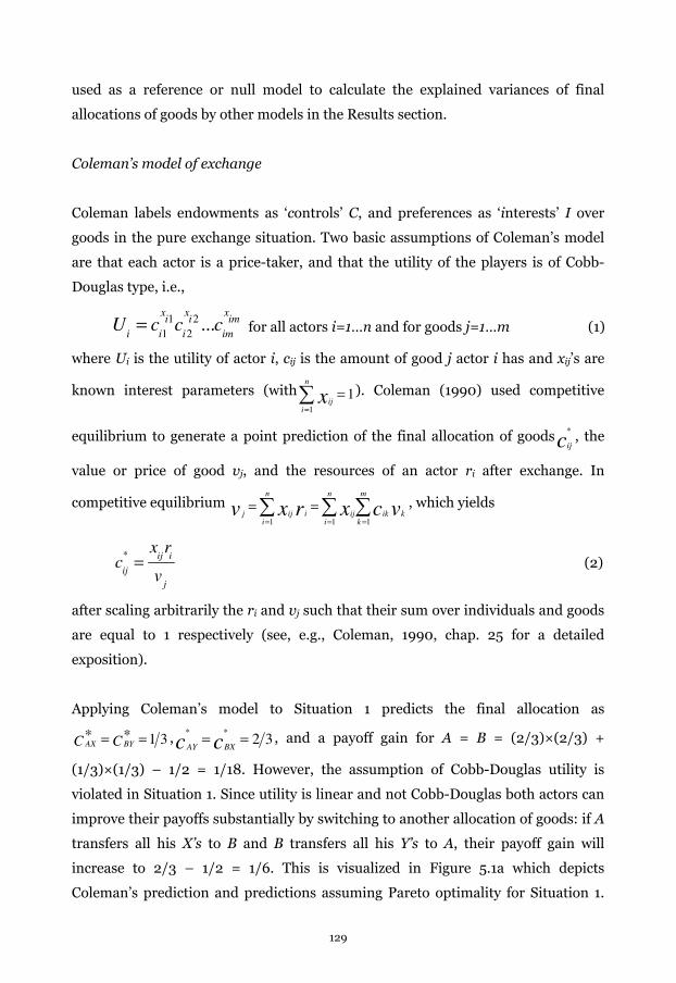
used as a reference or null model to calculate the explained variances of final
allocations of goods by other models in the Results section.
Coleman’s model of exchange
Coleman labels endowments as ‘controls’ C, and preferences as ‘interests’ I over
goods in the pure exchange situation. Two basic assumptions of Coleman’s model
are that each actor is a price-taker, and that the utility of the players is of Cobb-
Douglas type, i.e.,
1 2
1 2...
x x xi i im
i i i imU c c c= for all actors i=1…n and for goods j=1…m (1)
where Ui is the utility of actor i, cij is the amount of good j actor i has and xij’s are
known interest parameters (with 11
=∑=
n
iijx ). Coleman (1990) used competitive
equilibrium to generate a point prediction of the final allocation of goodscij
* , the
value or price of good vj, and the resources of an actor ri after exchange. In
competitive equilibrium vcxrxv k
m
kik
n
iij
n
iiijj ∑∑∑
===
==111
, which yields
* ij i
ij
j
x rc
v= (2)
after scaling arbitrarily the ri and vj such that their sum over individuals and goods
are equal to 1 respectively (see, e.g., Coleman, 1990, chap. 25 for a detailed
exposition).
Applying Coleman’s model to Situation 1 predicts the final allocation as
31== C*C*BYAX
, 32**
== cc BXAY, and a payoff gain for A = B = (2/3)×(2/3) +
(1/3)×(1/3) – 1/2 = 1/18. However, the assumption of Cobb-Douglas utility is
violated in Situation 1. Since utility is linear and not Cobb-Douglas both actors can
improve their payoffs substantially by switching to another allocation of goods: if A
transfers all his X’s to B and B transfers all his Y’s to A, their payoff gain will
increase to 2/3 – 1/2 = 1/6. This is visualized in Figure 5.1a which depicts
Coleman’s prediction and predictions assuming Pareto optimality for Situation 1.
129
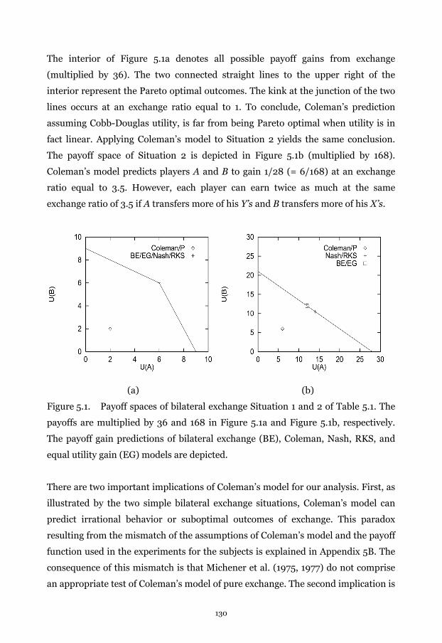
The interior of Figure 5.1a denotes all possible payoff gains from exchange
(multiplied by 36). The two connected straight lines to the upper right of the
interior represent the Pareto optimal outcomes. The kink at the junction of the two
lines occurs at an exchange ratio equal to 1. To conclude, Coleman’s prediction
assuming Cobb-Douglas utility, is far from being Pareto optimal when utility is in
fact linear. Applying Coleman’s model to Situation 2 yields the same conclusion.
The payoff space of Situation 2 is depicted in Figure 5.1b (multiplied by 168).
Coleman’s model predicts players A and B to gain 1/28 (= 6/168) at an exchange
ratio equal to 3.5. However, each player can earn twice as much at the same
exchange ratio of 3.5 if A transfers more of his Y’s and B transfers more of his X’s.
(a) (b)
Figure 5.1. Payoff spaces of bilateral exchange Situation 1 and 2 of Table 5.1. The
payoffs are multiplied by 36 and 168 in Figure 5.1a and Figure 5.1b, respectively.
The payoff gain predictions of bilateral exchange (BE), Coleman, Nash, RKS, and
equal utility gain (EG) models are depicted.
There are two important implications of Coleman’s model for our analysis. First, as
illustrated by the two simple bilateral exchange situations, Coleman’s model can
predict irrational behavior or suboptimal outcomes of exchange. This paradox
resulting from the mismatch of the assumptions of Coleman’s model and the payoff
function used in the experiments for the subjects is explained in Appendix 5B. The
consequence of this mismatch is that Michener et al. (1975, 1977) do not comprise
an appropriate test of Coleman’s model of pure exchange. The second implication is
130

that it predicts that each actor obtains from each good an amount equal to his
proportionate interest in that good if the value of resources is equal across actors:
using (2) and rA = rB we get xxcc BXAXBXAX=
** and xxcc BYAYBYAY
=**
. For
example in Situation 2 Coleman’s model predicts
3
2
9
8
7
3
7
4**=== xxcc BXAXBXAX
and 3
1
9
1
4
3
4
1**=== xxcc BYAYBYAY
because rA = rB = ½. If an actor has more resources than another actor, Coleman’s
model predicts that he obtains more than his proportionate interest in that good.
Proportional interest model
The proportionate interest (P) model predicts that the players have final controls
proportionate to their interest in the goods, i.e., *
1
/n
ij ij ijj
c x x=
= ∑ . Note that it does
not take into account the initial endowments. If the value of all actors’ resources is
equal, Coleman’s model and the P model provide the same predictions. Hence both
models predict the same allocations in situations 1 and 2. Consequently, also the P
model can predict irrational behavior or suboptimal outcomes of exchange (see also
Appendix 5B).
Models of cooperative bargaining
The core is based on two assumptions, individual rationality and weak Pareto-
optimality:
(i) The payoff vector 1
( ,..., )n
u u u= is individually rational i.e.
initial i N
i iu u≥ ∀ ∈ ,
(ii) u is weakly Pareto optimal i.e.
( ) where ( ) : { : : },n
u PO S PO S u S y R y u y S∈ = ∈ ∀ ∈ > ⇒ ∉
where S is a compact convex subset of Rn denoting the set of all payoff vectors that
can be the outcome of the bargaining. In the experiments, S is the set of all possible
payoff triplets or quadruplets that makes each player at least as well off as his
initial payoff. The core implies that after exchange there is no payoff vector which
makes all players better off.
131
Usually, the core contains a large (often infinite) set of payoff vectors. For example,
the core in the bilateral exchange situations of Table 5.1 is represented by the
straight lines in Figure 5.1a and 5.1b. The core of the pure exchange situations in
Michener et al’s studies are three-dimensional and four-dimensional spaces. To
make unique predictions on the set of core solutions, other cooperative game
theory solution concepts have been developed. These solutions select one solution
from the core that satisfies one or more reasonable or ‘fair’ requirements of a
solution.39 In the present study we use the Nash bargaining solution, the Rafai-
Kalai-Smorodinsky bargaining solution, and Myerson’s equal utility solution.
The Nash bargaining solution is the vector of utilities or payoffs that satisfies
1
( )arg max
n
i id s S i
s d≤ ∈ =
−∏ where <S, d> is a bargaining problem and i=1…n denotes the
players. S, as before, is a compact convex subset of Rn denoting the set of all payoff
vectors that can be the outcome of the bargaining, and d is the disagreement payoff
vector. The disagreement payoff vector, d, is the players’ payoff before exchange.
The Nash bargaining solutions in Figure 5.1a and 5.1b are (6, 6) and (14, 10.5),
respectively.
The Rafai-Kalai-Smorodinsky (RKS) solution is the intersection point of the
weakly Pareto optimal set, PO(S) as defined before, with the line that connects the
disagreement point, d, with the utopia point. The utopia point is defined as
1( , ) : (max{ : , },..., max{ : , })
nutopia S d x x S x d x x S x d= ∈ ≥ ∈ ≥ . So, the RKS solution is
found by defining the ray passing through the two points d and utopia(S,d) and
39 In theory, some models of cooperative bargaining, like Nash or equal utility gain, can
select more than one solution (e.g., see Heckathorn 1978). However, always one solution is
selected in the pure exchange situations here because of the linearity of the payoff space. For
an explanation of the set of requirements underlying the Nash and RKS bargaining
solutions, see Luce and Raiffa (1957) and Felsenthal and Diskin (1982).
132
then selecting the point at which this ray intersects with the core. The RKS
solutions are identical to the Nash solutions for both situations in Figure 5.1.40
The equal utility gain (EG) solution assumes that players only care about the
absolute utility increase of each player in an exchange situation. Formally, EG is the
solution to 1
max . . : ( ,..., )i i n
s t i u d and u u Sθ θ∀ = + ∈ . So, the EG solution is the
point where the unit vector, or the ray representing equal utility increments for all
players starting from the disagreement utilities, intersects with the core. The EG
solution predicts (6, 6) in Situation 1, and (12,12) in Situation 2.
Bilateral exchange model
Michener et al.’s experimental procedure only allowed for bilateral exchanges, and
not for agreements between three or more players. Nonetheless, the cooperative
solution concepts mentioned above assume that any coalition of players can be
formed for exchange. Because of this mismatch between the solution concepts and
the experimental procedure, an outcome of a pure exchange situation might not be
in the core, but still be ‘rationalizable’. For example, consider an example of
generalized exchange (e.g., Bearman, 1997) with three actors A, B, and C: A wants
what B has, B wants what C has, and C wants what A has. No profitable bilateral
exchange is possible; hence an outcome in which no exchange occurs is
rationalizable. However, the core solution predicts that each good is transferred to
the actor who wants it.
We employ a model of bilateral exchange that fits the experimental procedure. It is
based upon the model of collective decision-making developed by Stokman and van
Oosten (1994). The model detects and employs the exchange opportunities of
actors in the exchange situation. That is, it works on the micro level, whereas the
40 Assuming linear payoffs, payoff spaces of bilateral pure exchange situations in which one
good is exchanged for one other good either have one kink or no kink. It can be shown that
the Nash and RKS solutions are always equal if there is no kink, and are equal only under
certain conditions if there is a kink.
133
cooperative bargaining models are macro level models. It assumes that actors in a
collective decision-making situation bilaterally exchange voting positions in order
to affect the final outcome to their advantage. It uses the EG solution to specify the
ratio of each bilateral exchange. Generalizing Stokman and van Oosten’s (1994)
model to predict outcomes of pure exchange situations leads to the following
bilateral exchange (BE) algorithm consisting of two iterative steps:
(i) Conditional on the current allocation of endowments, construct a list
of mutually profitable bilateral exchange opportunities, ordered with
respect to payoff gain. If some exchange opportunities yield the same
profit, then order these exchanges randomly.
(ii) Execute the bilateral exchange opportunity on top of the list
Repeat steps (i) and (ii) until the list is empty.
If some exchange opportunities yield the same profit in step (i), the random order
determines the exchanges carried out and consequently the final allocations.
Therefore we ran the algorithm 1,000 times and calculated the final c* as the
average c* across these 1,000 runs.
It is assumed in the algorithm that actors give up and receive only one good in each
exchange. Note that the list can be ordered, because the EG solution specifies an
equal gain for both actors in the exchange. A strong assumption of the model is that
a less profitable exchange is carried out later than a more profitable exchange, even
if the two exchanges concern a pair of different actors. Finally, the model can be
said to assume bounded rationality of the actors: they do not take into account that
generalized exchange or perhaps another order of bilateral exchange might result
in a higher payoff for each actor.
Bounded rationality model
A bounded rationality model is developed to explain possible deviations from weak
Pareto optimality, either in the whole group (models of cooperative bargaining) or
in dyads (bilateral exchange model). To understand the distinction between
rationality and bounded rationality Kahneman (2003) distinguishes two cognitive
systems, each responsible for its own mode of thinking and deciding. These
134

systems are reasoning and intuition. Reasoning is done deliberately and effortfully,
but intuitive thoughts seem to come spontaneously to mind, without conscious
search or computation, and without effort (Kahneman, 2003, p.1450). While
rationality is associated with the reasoning system, bounded rationality is mainly
associated with the intuition system. Whether a task requires the intuition or
reasoning system is contingent on characteristics of the task. An important task
variable is task complexity. Task complexity has been shown to affect both actors’
preferences and decision-making behavior in many studies (e.g., Ho & Weigelt,
1996; Johnson & Payne, 1985; Swait & Adamowicz, 2001). It is generally
hypothesized in these studies that as task complexity increases, the accuracy of
decision-making heuristics decreases. There is a close relation between task
complexity and bounded rationality, as Ho and Weigelt (1996, p.660) explain:
“Task complexity and bounded rationality are flip sides of a coin. If players are fully
rational, task complexity is irrelevant because they can solve games of any
complexity. Conversely, games with trivial complexity can be solved by even
severely boundedly rational players.”
The participants in the pure exchange experiments of Michener et al. face a
complex task. There are many exchange opportunities between different actors in
which actors have to bargain to obtain a gain, and there is time pressure to close a
profitable deal with someone before someone else does. Therefore we hypothesize
that the participants might be inclined to employ heuristics, i.e., bounded
rationality. We distinguish three heuristics or strategies related to detecting
profitable bilateral exchange opportunities. Increasing in sophistication, these
strategies are:
(i) Exchange a good you do not want yourself for some good you value (‘zero’).
(ii) Exchange a good you want for some good you like more (‘absolute’).
(iii) Exchange a good you want for some good you like relatively more (‘relative’).
The ‘zero’ strategy requires hardly any reasoning. It requires actors to realize that
they can exchange goods for which their interest is zero for any other good they
value (interest larger than zero). The ‘absolute’ strategy requires a bit more
thinking. It requires actors to give away a good they value, while they obtain a good
they value more. Finally, the ‘relative’ strategy requires the most thinking, and in
135

fact comes down to rational behavior in bilateral exchange situations. It requires
actors to realize that profitable exchange is possible whenever the relative interest
of two actors for two goods differ. Note that the ‘relative’ strategy contains the
profitable opportunities detected by the ‘absolute’ strategy, and the ‘absolute’
strategy contains the opportunities detected by the ‘zero’ strategy. For example,
consider again exchange situations 1 and 2 presented in Table 5.1. The ‘zero’,
‘absolute’, ‘relative’ strategy detects no, one (situation 1), both profitable
opportunities, respectively. Finally, and most importantly, note that the BE model
assumes that actors use the fully rational ‘relative’ heuristic, whereas both the P
and Coleman model violate the ‘relative’ heuristic.
Many profitable bilateral exchange opportunities exist given the initial allocations
of endowments. These opportunities can be distinguished into different categories
which can be detected by one or more of the strategies identified above. We
distinguish the following four categories of exchange opportunities:
D0: Actors have different preference orders, and at least one actor has 0
interest in one good
S0: Actors have the same preference order, and one actor has 0 interest in one
good
Db: Actors have different preference orders, and both actors have interest in
both goods
Sb: Actors have the same preference order, and both actors have interest in
both goods
One only needs the least sophisticated heuristic to detect opportunity D0. One actor
can use the ‘zero’ strategy, the other either the ‘zero’ (in the case that both actors do
not value the good they offer) or ‘absolute’ strategy (if that actor values the good he
offers). Opportunity S0 is more difficult to detect; whereas one actor can use ‘zero’,
the other requires the most sophisticated ‘relative’ strategy to detect the
opportunity. However, we contend that it is sufficient if one of the two actors
detects the opportunity. Since the actor using ‘zero’ detects an opportunity S0
easily, he can make the opportunity salient to the other actor by offering many of
his valueless units in exchange for one of the other’s goods. In opportunity Db both
136

actors are required to use at least the ‘absolute’ strategy. Finally, both actors must
use the most sophisticated ‘relative’ strategy to detect Sb.
If actors are boundedly rational and use heuristics to detect profitable exchange
opportunities then some of these opportunities might go undetected. We expect, as
is generally hypothesized, that there is a negative relation between the task
complexity of detecting the opportunity and the proportion of these opportunities
that are detected and actually carried out. That is, at the end of the experiment, on
the basis of the final allocation of endowments, relatively more opportunities will
exist of those that are more difficult to detect. More formally, let fkB and fkE denote
the frequency of opportunities of type k at the Beginning and End of the
experiment, and rfk = fkE/fkB. Then the bounded rationality model implies:
Hypothesis 1: rfSb > rfDb > rfS0 > rfD0 .
Similarly, exchange opportunities that are difficult to detect might systematically
not be carried out in many experimental sessions, while those that are more easy to
detect, like S0 and D0, might accidentally not be carried out by some actors in only
some experimental sessions. Consequently, on average across all experimental
sessions we would expect a larger potential gain of exchanges at the end of the
experiment of opportunities that are difficult to detect than of opportunities that
are easy to detect. Let Xk denote the average potential gain of an exchange of
opportunity category k at the end of the experiment, then this hypothesis can be
formulated as:
Hypothesis 2: XSb > XDb > XS0 > XD0
The potential gain of each exchange opportunity is calculated by assuming the EG
solution.
5.3. Michener et al’s Experiments
Michener et al. (1975) investigated pure exchange systems consisting of three
actors exchanging four goods (1975) and four actors exchanging five goods (1977).
137

The experimental procedure was identical in both studies. Here, only a brief
summary with the essential details is provided.
In each study three pure exchange systems, called ‘configurations’ by Michener et
al, were investigated. Sixteen groups of three persons and 12 groups of four persons
were randomly assigned to each of the three configurations in the 1975 and 1977
study, respectively. Hence in total 144 subjects participated in each study.
After being seated around a table, the subjects were designated by name cards
(Alpha, Beta, Gamma, Delta). The subjects received colored poker chips, which
were in full view of all subjects. In total there were 400 or 500 chips, 100 of each
color. Before trading began, each subject received a sheet of paper indicating the
traders’ interest and initial control over chips. Hence the subjects had complete
information on all subjects’ payoffs. The interest and control matrix of each
configuration is depicted in Table 5.2a and Table 5.2b for the 1975 and 1977 study,
respectively. Michener et al. state that the interest and control values in all
configurations were randomly sampled, and rounded off to the nearest multiple of
ten.
Subjects were free to talk during the experiment. The experimenter left the room
and subjects were free to negotiate any trade bilaterally. No three-way or four-way
deals were permitted. Equilibrium was reached when all subjects decided that they
no longer wanted to trade or found that they could not promote any further trades
with the other subjects. Subjects earned a participation fee of $1 plus the money
earned in the experiment. The subjects’ payoff was linear in the endowments in the
following way: a subject received for each good an amount equal to (his interest for
the good) × (the number of units of the good he possesses) cents.
138
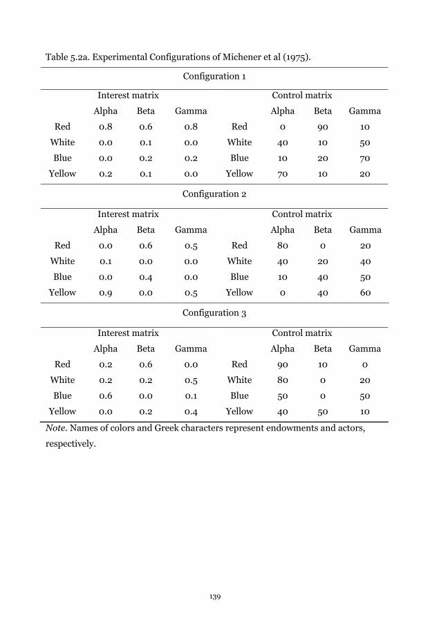
Table 5.2a. Experimental Configurations of Michener et al (1975).
Configuration 1
Interest matrix Control matrix
Alpha Beta Gamma Alpha Beta Gamma
Red 0.8 0.6 0.8 Red 0 90 10
White 0.0 0.1 0.0 White 40 10 50
Blue 0.0 0.2 0.2 Blue 10 20 70
Yellow 0.2 0.1 0.0 Yellow 70 10 20
Configuration 2
Interest matrix Control matrix
Alpha Beta Gamma Alpha Beta Gamma
Red 0.0 0.6 0.5 Red 80 0 20
White 0.1 0.0 0.0 White 40 20 40
Blue 0.0 0.4 0.0 Blue 10 40 50
Yellow 0.9 0.0 0.5 Yellow 0 40 60
Configuration 3
Interest matrix Control matrix
Alpha Beta Gamma Alpha Beta Gamma
Red 0.2 0.6 0.0 Red 90 10 0
White 0.2 0.2 0.5 White 80 0 20
Blue 0.6 0.0 0.1 Blue 50 0 50
Yellow 0.0 0.2 0.4 Yellow 40 50 10
Note. Names of colors and Greek characters represent endowments and actors,
respectively.
139

Table 5.2b. Experimental Configurations of Michener et al (1977)
Configuration 1
Interest matrix Control matrix
alpha beta gamma delta alpha beta gamma Delta
red 0.0 0.3 0.3 0.0 red 60 0 0 40
white 0.9 0.5 0.0 0.8 white 10 0 80 10
blue 0.1 0.0 0.0 0.0 blue 0 90 10 0
yellow 0.0 0.0 0.3 0.2 yellow 0 60 40 0
green 0.0 0.2 0.4 0.0 green 40 0 0 60
Configuration 2
Interest matrix Control matrix
alpha beta gamma delta alpha beta gamma delta
red 0.0 0.8 0.3 0.3 red 60 20 0 20
white 0.3 0.1 0.0 0.0 white 10 70 10 10
blue 0.1 0.1 0.0 0.0 blue 30 0 40 30
yellow 0.0 0.0 0.4 0.5 yellow 50 50 0 0
green 0.6 0.0 0.3 0.2 green 0 60 20 20
Configuration 3
Interest matrix Control matrix
alpha beta gamma delta alpha beta gamma delta
red 0.6 0.2 0.9 0.0 red 10 90 0 0
white 0.2 0.0 0.0 0.2 white 10 50 10 30
blue 0.2 0.4 0.1 0.0 blue 80 0 0 20
yellow 0.0 0.0 0.0 0.5 yellow 40 20 20 20
green 0.0 0.4 0.0 0.3 green 60 10 30 0
Note. Names of colors and Greek characters represent endowments and actors,
respectively.
140
5.4. Results
Approach
We focus on the final allocations c*. For each configuration we first calculated the
core. After calculating the core the Nash, RKS, and EG solutions were found. The
core is a convex surface in a three-dimensional (1975 paper) or a four-dimensional
(1977 paper) payoff space. The surface is spanned by a number of points. For
example, for Configuration 1 (C1) and C2 of the 1975 paper the core is the surface
that spans five points, for C3 eleven points span the surface. In Figure 5.2 the
solutions of the core (shaded area), Nash, RKS, EG, BE, Coleman, P, together with
the experimental results (open circles) are depicted for C1.41 Note that the
experimental results as well as the predictions of Coleman and P for this
configuration were not in the core. The P model even predicted Beta to lose 20
compared to his initial payoff.
Our analysis consisted of two steps. First we analyzed how much variance of the
final allocations was explained by the predictions of BE, Coleman, P, Nash, RKS,
and EG in the six configurations. Second, we tested our hypotheses on the
relationship between the complexity of the task to detect a mutually profitable
exchange and the type of exchange opportunity.
41 We do not include the core sets here because they are not easy to visualize, and since they
are big sets the core prediction is quite uninformative about the final outcome of the pure
exchange situation.
141

Figure 5.2. Payoff space of the pure exchange situation of Configuration 1 of
Michener et al. (1975). On the three axes the payoff gains are depicted of Alpha,
Beta, and Gamma. The shaded area represents the core, which here contains the
bilateral exchange (BE), Nash, RKS, and equal utility gain (EG) solution. The
experimental results (Exp) and the predictions of the proportional interest (P) and
Coleman model are also presented.
Explained variances
The proportion of variance (R2) of the final allocations of a configuration explained
by a model is the sum of squared deviations of this model’s predicted final
allocations and the observed final allocations, divided by the sum of squared
deviations of the initial and final allocations:
beta
alpha
gamma
142

∑∑ −
∑∑ −
= =
= ==
n
i
m
j
n
i
m
j
cc
ccR
ijij
ijij
1 1
2
1 1
2
2
)(
)(
initial*
model*
(3)
The models’ predictions of the final allocations for all configurations are shown in
Table 5A.1 to 5A.6 in the Appendix 5A. The denominator of (3) presents the sum of
squares of the null or no-exchange model considered by Michener et al. Dividing
this sum of squares by the number of actor-good combinations, equal to 12 and 20
for both studies, yields the variance not explained by the null model. The square
root of this number, the standard deviation, is presented in the top row of Table
5.3. The value of R2 for each model-configuration combination is presented in
Table 5.3, together with the average R2 of each model and of each configuration.
Note that no test could be performed comparing the R2 of different models, since
the models were not nested.
Table 5.3 Proportions of Variance Explained by the Solutions in all Configurations
1975 paper 1977 Paper
C1 C2 C3 C1 C2 C3 Average
SD 37.68 47.07 30.64 56.88 47.75 56.06
Coleman 0.68 0.99 0.86 0.91 0.96 0.96 0.89
Proportional 0.84 0.95 0.42 0.92 0.91 0.80 0.81
Nash 0.77 0.98 0.14 0.93 0.56 0.94 0.72
RKS 0.76 0.98 0.35 0.77 0.42 0.96 0.71
Egalitarian 0.77 0.95 0.41 0.84 0.38 0.98 0.72
Bilateral 0.78 0.98 0.85 0.99 0.94 0.94 0.91
Average 0.77 0.97 0.51 0.89 0.70 0.93 0.79
Note. The square root of the unexplained variances (SD) of each configuration is
presented in the top row. ‘Average’ represents the average of the variance explained
in a row or column.
The average R2 of the Coleman model was large, 0.89, and greater than the average
R2 of the P model, which was 0.81. Table 5.3 shows that all three models of
cooperative bargaining, Nash, RKS, and EG, performed on average worse than the
143

P and Coleman’s model. Their average R2 was 0.71 or 0.72. The three cooperative
bargaining models showed comparable performance in four configurations but
performed worse than Coleman’s model in C3 and C2 of the 1975 and 1977 paper,
respectively. In these configurations the differences in R2 were between 0.4 and
0.72 in favor of Coleman’s model. The BE model performed best with an average R2
equal to 0.91, although the difference with Coleman was small. The BE model also
performed much better than the cooperative bargaining models in C3 and C2 of the
1975 and 1977 papers, respectively.
Note that the performance of all solutions was good (R2’s from 0.89 to 0.97) in the
three configurations, C2 of the 1975 paper, and C1 and C3 of the 1977 paper. In fact,
the worst performance of all solutions in these configurations (R2 = 0.77) was not
worse than the best performance (also R2 = 0.77, of C1 of the 1975 paper) of the
three remaining configurations (C1 and C3 of 1975, and C2 of 1997). We attempt to
explain these differences in average performances across configurations in the
Discussion section.
Relationship between task complexity and type of exchange opportunity
Columns 2 to 4 of Table 5.4 represent the number of pure bilateral exchange
situations of each opportunity type in each configuration based on the initial
allocations, and between brackets those based on the final allocations. Initially
there were in total 88 profitable exchange opportunities among all possible actor
pair-good pair combinations.42 Of these 88, only 2 were of type Db, and 2 of type
Sb, the types that were hypothesized most difficult to detect (see column 8 of Table
5.4). At the end of the experiment, 20 opportunities existed (bottom of column 8),
of which only 13 were identical to those that existed initially. Hence 7 new
opportunities were created by the exchanges carried out by the participants in the
experiment. Of the 13 opportunities that remained at the end of the experiment, 2,
8, 1, and 2 were of type D0, S0, Db, and Sb respectively (numbers not shown in Table
42 There were in total 3×3×6 + 3×6×10 = 234 actor-good pair combinations (for each paper
these numbers represent configurations × actor pairs × good pairs).
144
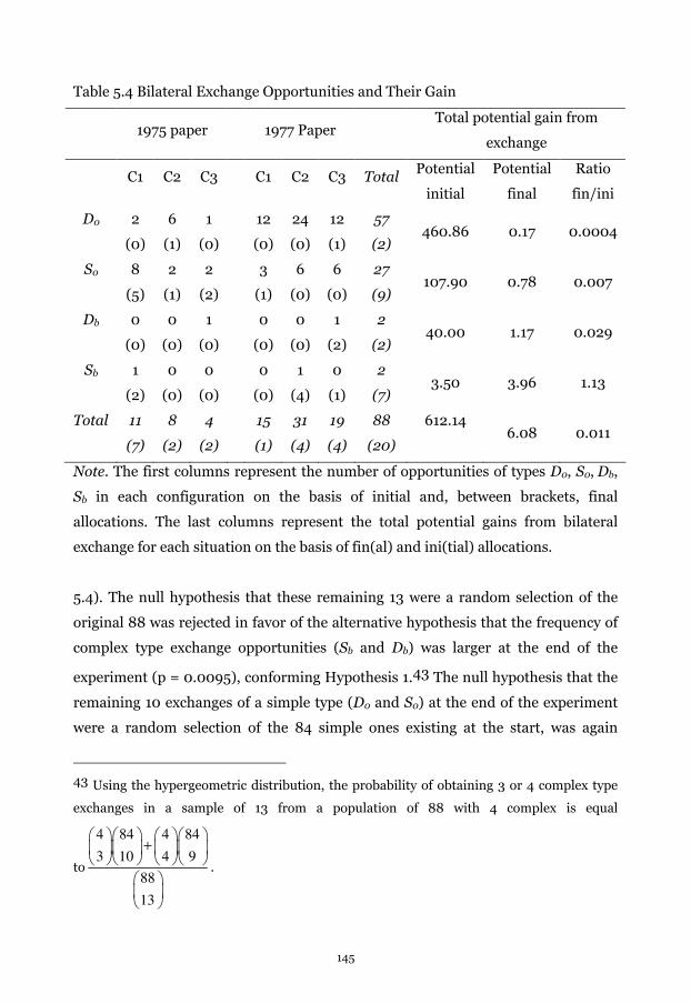
Table 5.4 Bilateral Exchange Opportunities and Their Gain
1975 paper 1977 Paper Total potential gain from
exchange
C1 C2 C3 C1 C2 C3 Total Potential
initial
Potential
final
Ratio
fin/ini
D0 2
(0)
6
(1)
1
(0)
12
(0)
24
(0)
12
(1)
57
(2) 460.86 0.17 0.0004
S0 8
(5)
2
(1)
2
(2)
3
(1)
6
(0)
6
(0)
27
(9) 107.90 0.78 0.007
Db 0
(0)
0
(0)
1
(0)
0
(0)
0
(0)
1
(2)
2
(2) 40.00 1.17 0.029
Sb 1
(2)
0
(0)
0
(0)
0
(0)
1
(4)
0
(1)
2
(7) 3.50 3.96 1.13
Total 11
(7)
8
(2)
4
(2)
15
(1)
31
(4)
19
(4)
88
(20)
612.14 6.08 0.011
Note. The first columns represent the number of opportunities of types D0, S0, Db,
Sb in each configuration on the basis of initial and, between brackets, final
allocations. The last columns represent the total potential gains from bilateral
exchange for each situation on the basis of fin(al) and ini(tial) allocations.
5.4). The null hypothesis that these remaining 13 were a random selection of the
original 88 was rejected in favor of the alternative hypothesis that the frequency of
complex type exchange opportunities (Sb and Db) was larger at the end of the
experiment (p = 0.0095), conforming Hypothesis 1.43 The null hypothesis that the
remaining 10 exchanges of a simple type (D0 and S0) at the end of the experiment
were a random selection of the 84 simple ones existing at the start, was again
43 Using the hypergeometric distribution, the probability of obtaining 3 or 4 complex type
exchanges in a sample of 13 from a population of 88 with 4 complex is equal
to
4 84 4 84
3 10 4 9
88
13
+
.
145
rejected in favor of the hypothesis that the relative frequency of the more complex
type S0 at the end was larger (p = 0.0014).44 Finally, of the 7 newly created
exchange opportunities 0, 1, 1, and 5 were of type D0, S0, Db, and Sb respectively
(numbers not shown in Table 5.4). If one hypothesizes Sb as likely to occur as each
of the other types, then this hypothesis is rejected with a binomial test (p = 0.008).
This result is also in line with our first hypothesis that there is a positive
relationship between the difficulty to detect an opportunity and its occurrence at
the end of the experiment.
Let us now focus on our second hypothesis on the size of the average potential gain
from exchange opportunities based on the initial and final allocations. The average
potential gains at the end of the experiment were 0.085, 0.087, 0.584, and 0.566
for type D0, S0, Db, Sb, respectively. An average was obtained by calculating the
average potential gain of all exchange opportunities remaining at the end of the
experiments across all six experimental configurations. The number of
opportunities for each type was 2, 9, 2, and 7 for type D0, S0, Db, and Sb respectively
(see 8th column of Table 5.4). These numbers are too small to perform a powerful
test on Hypothesis 2. However, comparing the simple types D0 and S0 to the
complex types led to the conclusion that the combined average potential gain for
the complex types Sb and Db was larger than for the simple types (t = -3.488, df =
8.63, p = 0.004, one-tailed) corroborating Hypothesis 2. Note, however, that the
average potential gains at the end were substantially smaller than at the start of the
experiment. Of the 88 opportunities at the start, an opportunity’s potential gain
was smaller than 1 for only 2 opportunities, while out of 20 opportunities at the end
the potential gain was larger than 1 for only 2 opportunities (both of most complex
type Sb).
44 Using the hypergeometric distribution, the probability of obtaining 2 or less D0 exchanges
in a sample of 10 from a population of 84 with 57 of type D0 is equal
to
57 27 57 27 57 27
2 8 1 9 0 10
84
10
+ +
.
146
Additional evidence for both hypotheses on the relation between task complexity
and the likelihood of carrying out different exchange opportunities comes from
columns 9 to 11 of Table 5.4. The 9th column of Table 5.4 represents the total
potential gains from bilateral exchange opportunities for each type in the initial
allocation across all experimental configurations, i.e., the sum of all potential gains
of all exchange opportunities of each type that existed at the start of the
experiment. Note that this number by itself is not meaningful since not all of these
exchanges can be carried out simultaneously. This number is a combination of both
the size of the average potential gain and the frequency of each exchange
opportunity type. The 10th column shows the same numbers for the final
allocations, the 11th column shows the ratio of these numbers to those of the 9th
column. Note that the ratios in the 11th column increase in task complexity of the
exchange type, which is in agreement with both hypotheses. The potential gain for
most complex type Sb was even 1.13 times larger at the end than at the start of the
experiment. While at the start of the experiment the relative potential for Sb was
only 3.5/612.14 = 0.006, and 0.071 for Sb and Db together, at the end it was
3.96/6.08 = 0.651 (and 0.856 for Sb and Db together).
5.5. Discussion
In this section we attempt to provide an explanation of the fit of the models to the
data of all six configurations, by analyzing the properties of the configurations and
the models applied to them. We first start with the configurations of which the final
allocations were fitted well by all models, then the configurations are discussed
where cooperative bargaining models failed to explain the final allocations.
The models’ average fit was between 0.89 and 0.97 in C2 of 1975 and C1 and C3 of
1977, substantially better than in the other three configurations. A relatively
straightforward explanation of this good fit can be provided for two of these
configurations: C2 of 1975 and C1 of 1997. Only for these configurations the initial
exchange opportunities consisted only of simple type (D0 and S0). If all exchange
opportunities are of a simple type then the core spans a smaller area, because all
147

points in the core correspond to allocations in which actors having no interest in a
good obtain nothing of that good. Nash, RKS, and EG are necessarily in the core.
Coleman’s model and the P model also predict that the actors having no interest in
a good do not have that good, which makes Coleman and P solutions close to the
core if not in. For C2 and C3 of 1977 these solutions were in fact in the core.
Moreover, final allocations were also in the core because actors could detect the
exchanges of a simple type using the least sophisticated ‘zero’ heuristic, and by
carrying out these opportunities no profitable exchange opportunity remained at
the end of the experiment.
An ad hoc explanation for the very good fit for C3 of 1977 is that there was only one
exchange opportunity of complex type Db, which was not that hard to detect. This
one opportunity was likely to be a focal exchange opportunity for two reasons.
First, it involved Red and White, the goods in which all actors were most interested.
Second, of all exchange opportunities present at the start of the experiment, the
opportunity Db had the largest potential gain. Because this exchange opportunity
was likely to be detected, it was likely to be carried out, as predicted by all rational
models of exchange.
The models’ average fit was substantially smaller for the other three configurations.
In particular, the fit of the cooperative bargaining models was poor in C3 of 1975
and C2 of 1977 (see Table 5.3). The superior performance of the BE model over the
other models’ performance in these configurations suggests that there was a
difference in ‘pair rationality’ or Pareto optimality at the level of dyads as assumed
in the BE model, and group rationality or (weak) Pareto optimality at the level of
the whole group as assumed in the cooperative bargaining models. Consider first
C3 of the 1975 paper. The final allocation matrix (top of Table 5A.3) and the
interest matrix (Table 5.2a, bottom and left) reveal that all three actors could not
improve their payoffs much by exchanging bilaterally, but they could have done so
by generalized exchange. If Alpha had transferred Red to Beta, Beta had transferred
Yellow to Gamma, and Gamma had transferred White to Alpha, all actors’ payoffs
would improve significantly. Hence, as predicted by the BE model, not all
148

participants did carry out the generalized exchange, falsifying the cooperative
bargaining models.45
Although we did not find evidence for generalized exchange in these pure exchange
experiments, this does not imply that actors never did it. Indeed, there exists both
empirical and ecological evidence of generalized exchange in the sociological
literature (e.g., Bearman, 1997; Yamagishi & Cook, 1993). The explanation of why
generalized exchange was not carried out by all participants can be found in task
complexity. Previous research on task complexity revealed that as task complexity
increases, decision-making becomes less sophisticated and easy heuristics are used.
The participants in the experiments face a complex environment containing many
exchange opportunities, of which many are easy to detect, and some, in particular
the generalized exchange opportunity, difficult to detect. Hence participants
carried out the ones that were easy to detect with the easy heuristics, and not the
generalized exchange. However, if the only exchange opportunity that exists is
generalized exchange, then the complexity of the task is reduced and one can
expect this generalized exchange to be carried out by some groups of actors, as is
indeed observed in experimental studies (Cook & Yamagishi, 1993).
The misfit of the cooperative bargaining solutions for C2 of 1977 might have
resulted from not taking into account differences in exchange opportunities
between actors in the pure exchange situation, as in exchange networks. C2 can be
represented by a Stem exchange network, Alpha, Beta, Delta forming a triangle,
and Gamma only connected to Alpha. Alpha has two alternative exchange relations
with Beta and Delta that are also more valuable to him than his relation with
Gamma. Alpha’s relation with Delta is more valuable because Delta pays a better
price for the Yellow of Alpha since Delta is more interested in the Yellow than
Gamma. Alpha’s relation with Beta is more valuable since Beta pays a better price
for Red than Gamma. Since Alpha cannot exchange with Gamma and the other two
partners at the same time (all his Yellow and Red were sold to Beta and Delta),
45 The predictions of the P model were unreasonable for this configuration, and
performance bad, because it predicted Alpha to lose points.
149

Gamma is excluded from an exchange yielding substantial gain. Table 5A.5 reveals
that Alpha and Beta obtained a substantially higher payoff in the experiment than
predicted by the cooperative bargaining solutions, and Gamma substantially less.
The BE model yielded a very good fit (R2 = 0.94) and predicted that Gamma is
excluded from an exchange yielding substantial gain. However, this asymmetry in
gains because of differences in exchange opportunities was not predicted by the
cooperative bargaining models because they do not take into account possible
exclusion from exchange.
The Coleman and P model also predicted accurately the final allocations in C2 of
the 1977 paper, however, for other reasons than the BE model. The P model
predicted Alpha’s and Beta’s relative advantage because their proportional interests
were larger than those of Gamma and Delta. Coleman’s model accurately predicted
an even larger relative advantage of Alpha and Beta because they had more
resources than Gamma (resources were 0.336, 0.398, 0.096, 0.169, for Alpha to
Delta, respectively).
The third and last configuration for which average performance was not very good
(R2 = 0.77) was C1 of the 1975 paper. This performance can partly be explained by
the fact that the sum of potential gains from exchanging in this configuration
(19.26) were smaller than in the other configurations (39.71 for C3 of 1975, and >
100 for the others), and by the presence of two opportunities of most complex type
Sa. We conclude by noting that, although the P model fitted best, the P model as
well as the Coleman model generated a prediction that is nonsensical. The P model
predicted Beta to lose more than 20 payoff points (see Table 5A.1). Coleman’s
model predicted Alpha to end up with less Yellow than he started with. This implies
that Alpha was predicted to engage in an exchange yielding a negative payoff,
because of all actors Alpha is relatively most interested in Yellow. Both models’
nonsensical predictions result from two factors. First, the initially skewed
distribution of resources in favor of Beta (Beta’s resources were 0.653, almost twice
as much as the resources of Alpha and Gamma combined) were not taken into
account by the P model. Second, both models’ predictions are in line with the
‘absolute’ heuristic, and not the ‘relative’ heuristic; both models predict actors to
150

end up with more of the good they like most, instead of ending up with the good
they like most relatively.
Finally, the fit of models’ predictions cannot be explained by the possibility of
actors behaving rationally in each session, whereas the average across all sessions
is not in the core. Although it is true that the core is, by definition, a convex space,
and the average of some points in this space might lie below it; the experiments’
results ruled out this possible alternative explanation. For example, the data clearly
revealed that the actors did not engage in generalized exchange in at least one
configuration. As another example, consider C1 of 1975. Its final configuration can
only be explained by assuming that actors were reluctant to give up the good that
they liked most, thereby violating the fully rational ‘relative’ heuristic. All points in
the core correspond to Beta having all the Blue and Alpha having some Yellow
before having any Red. The actors were most interested in Red. In the experiments
did not exchange Red for their relatively most preferred good, which is evidence
that many participants used the ‘absolute’ heuristic, i.e., focus on getting as much
of what they like most, instead of the ‘relative’ heuristic. Consequently, Beta did not
end up having all the Blue and Alpha did not have any Yellow. The use of the
‘absolute’ heuristic instead of the ‘relative’ heuristic is in line with Coleman’s and
the P model, and partly explains these models’ good fit in many configurations.
5.6. Conclusion
The goal of the present paper was to explain human behavior in pure exchange
situations. The data of the pure exchange experiments of Michener, Cohen and
Sørenson (1975, 1977) were reanalyzed with models that differ to the extent they
assume behavior to be rational. First, cooperative bargaining models were applied
that assume group rationality or weak Pareto optimality at the group level. Second,
a bilateral exchange model was applied assuming Pareto optimality at the dyadic
level. The bilateral exchange model is an adaptation of Stokman van Oosten’s
(1994) model to forecast outcomes of collective decision making. The model was
developed because in the experimental procedure participants were only allowed to
exchange bilaterally. Third, a model was applied assuming bounded rational actors
151
who apply heuristics to detect mutually profitable exchange opportunities. The
heuristics were linked to the task complexity of four exchange opportunity
categories, i.e., the difficulty to detect whether each of these categories can give rise
to mutually profitable exchanges.
On average, the models could predict the final allocations from reasonably well to
very well, with the best performance by the bilateral exchange model. This good
performance in combination with the observation that only very few profitable
exchange opportunities remained at the end of the experiments suggests that
actors’ behavior in pure exchange situations is rational at the dyadic level, i.e., leads
to Pareto optimal outcomes in bilateral exchange. However, evidence for deviations
from rational behavior was obtained confirming our hypothesis on the relation
between the sophistication needed to detect the opportunity and the likelihood that
it is carried out. It turned out that participants were less likely to give up a good
they like most, thereby violating the ‘relative’ heuristic, and used the less
sophisticated ‘zero’ and ‘absolute’ heuristics corresponding to boundedly rational
behavior. This finding agrees with the P and Coleman’s model that also violate the
‘relative’ heuristic. This might partly explain the good fit of these models, although
these models were shown to generate nonsensical predictions in some pure
exchange situations.
While there existed opportunities that could only be detected by the most
sophisticated ‘relative’ heuristic corresponding to rational behavior, almost all
opportunities in the experiments could be detected by the ’zero’ and ‘absolute’
heuristics corresponding to boundedly rational behavior. This explains the
seemingly inconsistent result that the bilateral exchange model fitted very well
although evidence for deviations of dyadic rationality was found. Finally, actors did
not carry out some generalized exchanges, and evidence was found that exchange
opportunities lead to large differences in actors’ payoffs, as in some exchange
networks. These two results were accurately predicted by the bilateral exchange
model, but were not anticipated by the cooperative bargaining models. However,
we note that only by analyzing the data with the cooperative bargaining models we
152

could detect these and other deviations from rationality in the experiments in the
first place.
For future research we have two suggestions. The first suggestion is to study
systematically the effect of type of exchange opportunity on the frequency with
which these different types are carried out, and on their outcomes. In Michener et
al’s data there were only a few opportunities of complex type. In particular, more
opportunities of complex types need to be investigated and compared to simple
types in order to obtain more insight on how pure exchange is carried out. A second
suggestion for future research would be to study pure exchange in the context of
exchange networks. The results of the current study suggest that not all pure
exchanges are alike, some are more cognitive complex than others. In the exchange
network literature, an (bilateral) exchange is defined as the opportunity to split a
common resource pool of fixed size, usually 24 points. This split is a representation
of exchange of low cognitive complexity. Since we found that the cognitive
complexity of an exchange opportunity decreased the likelihood or extent to which
it was carried out, it might be that the effect of network structure on the outcome of
exchange interacts with the cognitive complexity of the relations embedded in this
network. For example, an actor having relatively many opportunities of a complex
type might have difficulties detecting and carrying out these opportunities, while an
actor having opportunities of a simple type might not.
153
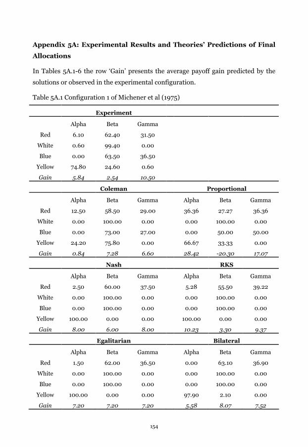
Appendix 5A: Experimental Results and Theories’ Predictions of Final
Allocations
In Tables 5A.1-6 the row ‘Gain’ presents the average payoff gain predicted by the
solutions or observed in the experimental configuration.
Table 5A.1 Configuration 1 of Michener et al (1975)
Experiment
Alpha Beta Gamma
Red 6.10 62.40 31.50
White 0.60 99.40 0.00
Blue 0.00 63.50 36.50
Yellow 74.80 24.60 0.60
Gain 5.84 2.54 10.50
Coleman Proportional
Alpha Beta Gamma Alpha Beta Gamma
Red 12.50 58.50 29.00 36.36 27.27 36.36
White 0.00 100.00 0.00 0.00 100.00 0.00
Blue 0.00 73.00 27.00 0.00 50.00 50.00
Yellow 24.20 75.80 0.00 66.67 33.33 0.00
Gain 0.84 7.28 6.60 28.42 -20.30 17.07
Nash RKS
Alpha Beta Gamma Alpha Beta Gamma
Red 2.50 60.00 37.50 5.28 55.50 39.22
White 0.00 100.00 0.00 0.00 100.00 0.00
Blue 0.00 100.00 0.00 0.00 100.00 0.00
Yellow 100.00 0.00 0.00 100.00 0.00 0.00
Gain 8.00 6.00 8.00 10.23 3.30 9.37
Egalitarian Bilateral
Alpha Beta Gamma Alpha Beta Gamma
Red 1.50 62.00 36.50 0.00 63.10 36.90
White 0.00 100.00 0.00 0.00 100.00 0.00
Blue 0.00 100.00 0.00 0.00 100.00 0.00
Yellow 100.00 0.00 0.00 97.90 2.10 0.00
Gain 7.20 7.20 7.20 5.58 8.07 7.52
154

Table 5A.2 Configuration 2 of Michener et al (1975)
Experiment
Alpha Beta Gamma
Red 0.00 28.90 71.10
White 99.80 0.10 0.10
Blue 0.30 99.70 0.00
Yellow 56.20 0.00 43.80
Gain 56.56 41.22 17.45
Coleman Proportional
Alpha Beta Gamma Alpha Beta Gamma
Red 0.00 40.40 59.60 0.00 54.55 45.45
White 100.00 0.00 0.00 100.00 0.00 0.00
Blue 0.00 100.00 0.00 0.00 100.00 0.00
Yellow 56.50 0.00 43.50 64.29 0.00 35.71
Gain 56.85 48.24 11.55 63.86 56.73 0.58
Nash RKS
Alpha Beta Gamma Alpha Beta Gamma
Red 0.00 15.56 84.44 0.00 23.64 76.36
White 100.00 0.00 0.00 100.00 0.00 0.00
Blue 0.00 100.00 0.00 0.00 100.00 0.00
Yellow 48.89 0.00 51.11 41.82 0.00 58.18
Gain 50.00 33.33 27.78 43.64 38.18 27.27
Egalitarian Bilateral
Alpha Beta Gamma Alpha Beta Gamma
Red 0.00 18.14 81.86 0.00 41.82 58.18
White 100.00 0.00 0.00 100.00 0.00 0.00
Blue 0.00 100.00 0.00 5.00 95.00 0.00
Yellow 32.09 0.00 67.91 44.29 0.00 55.71
Gain 34.88 34.88 34.88 45.86 47.09 16.95
155
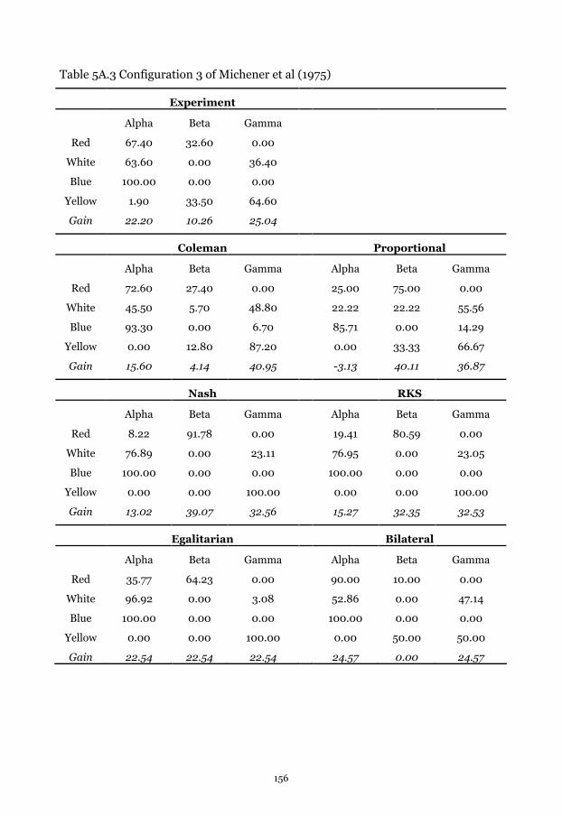
Table 5A.3 Configuration 3 of Michener et al (1975)
Experiment
Alpha Beta Gamma
Red 67.40 32.60 0.00
White 63.60 0.00 36.40
Blue 100.00 0.00 0.00
Yellow 1.90 33.50 64.60
Gain 22.20 10.26 25.04
Coleman Proportional
Alpha Beta Gamma Alpha Beta Gamma
Red 72.60 27.40 0.00 25.00 75.00 0.00
White 45.50 5.70 48.80 22.22 22.22 55.56
Blue 93.30 0.00 6.70 85.71 0.00 14.29
Yellow 0.00 12.80 87.20 0.00 33.33 66.67
Gain 15.60 4.14 40.95 -3.13 40.11 36.87
Nash RKS
Alpha Beta Gamma Alpha Beta Gamma
Red 8.22 91.78 0.00 19.41 80.59 0.00
White 76.89 0.00 23.11 76.95 0.00 23.05
Blue 100.00 0.00 0.00 100.00 0.00 0.00
Yellow 0.00 0.00 100.00 0.00 0.00 100.00
Gain 13.02 39.07 32.56 15.27 32.35 32.53
Egalitarian Bilateral
Alpha Beta Gamma Alpha Beta Gamma
Red 35.77 64.23 0.00 90.00 10.00 0.00
White 96.92 0.00 3.08 52.86 0.00 47.14
Blue 100.00 0.00 0.00 100.00 0.00 0.00
Yellow 0.00 0.00 100.00 0.00 50.00 50.00
Gain 22.54 22.54 22.54 24.57 0.00 24.57
156
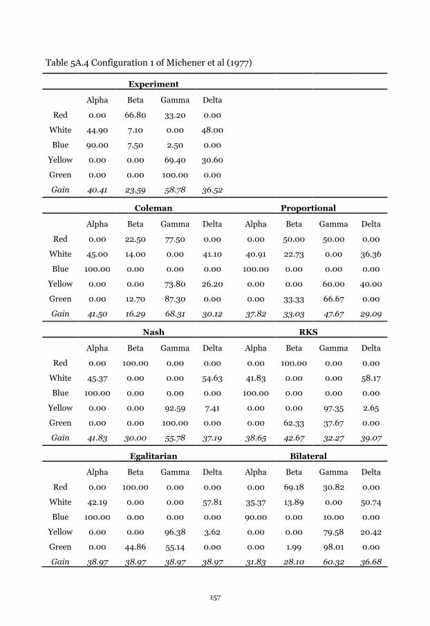
Table 5A.4 Configuration 1 of Michener et al (1977)
Experiment
Alpha Beta Gamma Delta
Red 0.00 66.80 33.20 0.00
White 44.90 7.10 0.00 48.00
Blue 90.00 7.50 2.50 0.00
Yellow 0.00 0.00 69.40 30.60
Green 0.00 0.00 100.00 0.00
Gain 40.41 23.59 58.78 36.52
Coleman Proportional
Alpha Beta Gamma Delta Alpha Beta Gamma Delta
Red 0.00 22.50 77.50 0.00 0.00 50.00 50.00 0.00
White 45.00 14.00 0.00 41.10 40.91 22.73 0.00 36.36
Blue 100.00 0.00 0.00 0.00 100.00 0.00 0.00 0.00
Yellow 0.00 0.00 73.80 26.20 0.00 0.00 60.00 40.00
Green 0.00 12.70 87.30 0.00 0.00 33.33 66.67 0.00
Gain 41.50 16.29 68.31 30.12 37.82 33.03 47.67 29.09
Nash RKS
Alpha Beta Gamma Delta Alpha Beta Gamma Delta
Red 0.00 100.00 0.00 0.00 0.00 100.00 0.00 0.00
White 45.37 0.00 0.00 54.63 41.83 0.00 0.00 58.17
Blue 100.00 0.00 0.00 0.00 100.00 0.00 0.00 0.00
Yellow 0.00 0.00 92.59 7.41 0.00 0.00 97.35 2.65
Green 0.00 0.00 100.00 0.00 0.00 62.33 37.67 0.00
Gain 41.83 30.00 55.78 37.19 38.65 42.67 32.27 39.07
Egalitarian Bilateral
Alpha Beta Gamma Delta Alpha Beta Gamma Delta
Red 0.00 100.00 0.00 0.00 0.00 69.18 30.82 0.00
White 42.19 0.00 0.00 57.81 35.37 13.89 0.00 50.74
Blue 100.00 0.00 0.00 0.00 90.00 0.00 10.00 0.00
Yellow 0.00 0.00 96.38 3.62 0.00 0.00 79.58 20.42
Green 0.00 44.86 55.14 0.00 0.00 1.99 98.01 0.00
Gain 38.97 38.97 38.97 38.97 31.83 28.10 60.32 36.68
157

Table 5A.5 Configuration 2 of Michener et al (1977)
Experiment
Alpha Beta Gamma Delta
Red 0.00 93.20 2.60 4.20
White 81.70 18.30 0.00 0.00
Blue 24.80 75.20 0.00 0.00
Yellow 0.00 0.00 43.30 56.70
Green 79.40 0.00 13.20 7.40
Gain 68.63 60.91 16.06 21.09
Coleman Proportional
Alpha Beta Gamma Delta Alpha Beta Gamma Delta
Red 0.00 80.00 7.30 12.70 0.00 57.14 21.43 21.43
White 71.70 28.30 0.00 0.00 75.00 25.00 0.00 0.00
Blue 45.80 54.20 0.00 0.00 50.00 50.00 0.00 0.00
Yellow 0.00 0.00 31.40 68.60 0.00 0.00 44.44 55.56
Green 76.30 0.00 10.90 12.80 54.55 0.00 27.27 18.18
Gain 65.87 49.25 12.02 30.67 54.23 30.21 26.39 27.84
Nash RKS
Alpha Beta Gamma Delta Alpha Beta Gamma Delta
Red 0.00 100.00 0.00 0.00 0.00 68.54 31.46 0.00
White 100.00 0.00 0.00 0.00 100.00 0.00 0.00 0.00
Blue 100.00 0.00 0.00 0.00 100.00 0.00 0.00 0.00
Yellow 0.00 0.00 19.17 80.83 0.00 0.00 10.44 89.56
Green 24.44 0.00 75.56 0.00 9.47 0.00 90.53 0.00
Gain 48.66 57.00 24.34 30.42 39.68 21.83 34.77 34.78
Egalitarian Bilateral
Alpha Beta Gamma Delta Alpha Beta Gamma Delta
Red 0.00 72.85 27.15 0.00 0.00 100.00 0.00 0.00
White 100.00 0.00 0.00 0.00 95.00 5.00 0.00 0.00
Blue 100.00 0.00 0.00 0.00 0.00 100.00 0.00 0.00
Yellow 0.00 0.00 9.44 90.56 0.00 0.00 24.45 75.55
Green 2.13 0.00 97.87 0.00 74.11 0.00 25.89 0.00
Gain 35.28 35.28 35.28 35.28 66.97 67.50 11.55 27.78
158
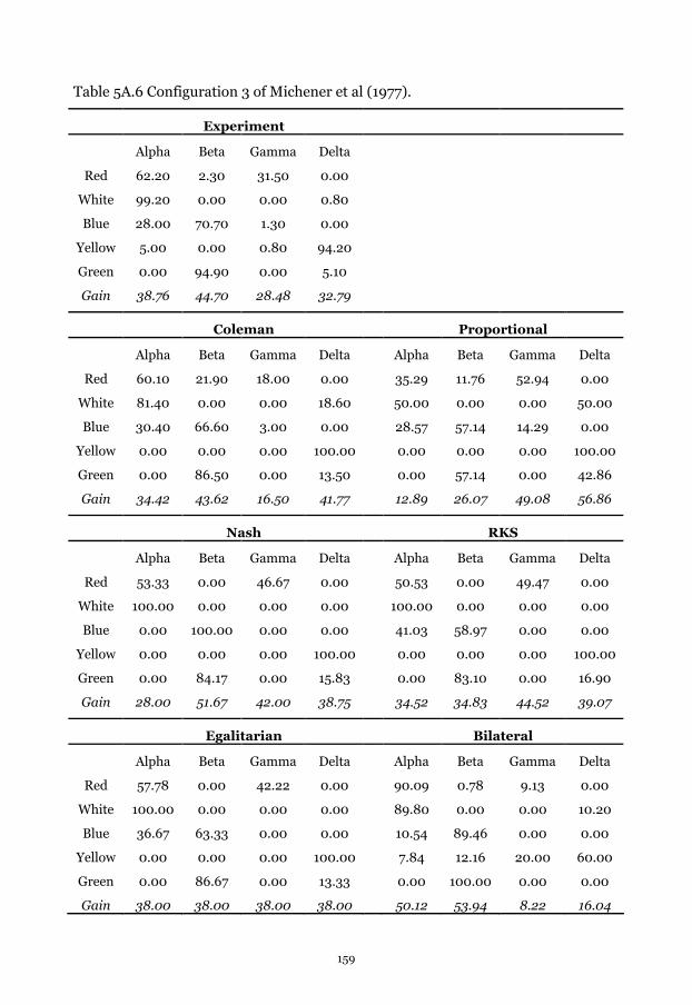
Table 5A.6 Configuration 3 of Michener et al (1977).
Experiment
Alpha Beta Gamma Delta
Red 62.20 2.30 31.50 0.00
White 99.20 0.00 0.00 0.80
Blue 28.00 70.70 1.30 0.00
Yellow 5.00 0.00 0.80 94.20
Green 0.00 94.90 0.00 5.10
Gain 38.76 44.70 28.48 32.79
Coleman Proportional
Alpha Beta Gamma Delta Alpha Beta Gamma Delta
Red 60.10 21.90 18.00 0.00 35.29 11.76 52.94 0.00
White 81.40 0.00 0.00 18.60 50.00 0.00 0.00 50.00
Blue 30.40 66.60 3.00 0.00 28.57 57.14 14.29 0.00
Yellow 0.00 0.00 0.00 100.00 0.00 0.00 0.00 100.00
Green 0.00 86.50 0.00 13.50 0.00 57.14 0.00 42.86
Gain 34.42 43.62 16.50 41.77 12.89 26.07 49.08 56.86
Nash RKS
Alpha Beta Gamma Delta Alpha Beta Gamma Delta
Red 53.33 0.00 46.67 0.00 50.53 0.00 49.47 0.00
White 100.00 0.00 0.00 0.00 100.00 0.00 0.00 0.00
Blue 0.00 100.00 0.00 0.00 41.03 58.97 0.00 0.00
Yellow 0.00 0.00 0.00 100.00 0.00 0.00 0.00 100.00
Green 0.00 84.17 0.00 15.83 0.00 83.10 0.00 16.90
Gain 28.00 51.67 42.00 38.75 34.52 34.83 44.52 39.07
Egalitarian Bilateral
Alpha Beta Gamma Delta Alpha Beta Gamma Delta
Red 57.78 0.00 42.22 0.00 90.09 0.78 9.13 0.00
White 100.00 0.00 0.00 0.00 89.80 0.00 0.00 10.20
Blue 36.67 63.33 0.00 0.00 10.54 89.46 0.00 0.00
Yellow 0.00 0.00 0.00 100.00 7.84 12.16 20.00 60.00
Green 0.00 86.67 0.00 13.33 0.00 100.00 0.00 0.00
Gain 38.00 38.00 38.00 38.00 50.12 53.94 8.22 16.04
159
Appendix 5B. Michener et al.’s Experiments and Coleman’s Model
The goal of Michener et al. (1975, 1977) was to test Coleman’s model of exchange in
the lab. Their studies do not comprise an appropriate test of the model because of a
mismatch between the assumed utility function and the payoff function used in the
experiment. Coleman’s model assumes Cobb-Douglas utility (see Equation 1),
which implies decreasing marginal utility, whereas the payoffs in Michener et al.’s
experiment were linear in the quantities of the goods possessed by the actors. That
is, each additional unit of a good provides less additional utility in Coleman’s model
while it provides the same additional payoff in Michener et al.’s experiments.
Because of this misspecification Coleman’s model predicts irrational behaviour and
suboptimal outcomes of exchange in Michener et al.’s experiments.
The first step in order to understand this paradox is the realization that the use of
linear payoffs results in extreme allocations of endowments if rational behavior is
assumed. That is, at least one of two actors will transfer all units of his good in a
bilateral exchange situation. For example, the Pareto optimal allocations in
Situation 2 correspond to exchanges in which A transfers all of his Y to B, other
exchanges are suboptimal. However, a consequence of using Cobb-Douglas utility
is that Coleman’s model predicts final allocations in which actors always keep some
of a good if they are interested in it, which is suboptimal.
Applying Coleman’s model to situations 1 and 2 led to suboptimal outcomes, but
these outcomes were still an improvement relative to the initial allocation.
However, it is easy to construct bilateral exchange situations with linear payoffs
where Coleman’s model predicts all actors to lose. For example, consider the 3-
event 3-actor exchange system (actors 1,2,3, goods D,E,F) with c1D = c2E = c3F = 1,
x1D = x2E = x3F = 0.6, x1F = x2D = x3E = 0.4, and all other values of x and c equal to 0.
Since all actors already have all of the good they want most, their payoff is already
maximized. Because all actors’ resources are equal and all goods are equally
valuable, Coleman’s model predicts final allocations equal to the interests: c1D = c2E
= c3F = 0.6, c1D = c2E = c3F = 0.4. This final allocation amounts to a loss in payoffs
for all actors equal to 0.4×0.6 = 0.24, or 40% of their initial payoff. Note that the P
model produces the same nonsensical prediction for this 3-event 3-actor exchange
system.
160

Chapter 6
Conclusions
This thesis studies network formation and exchange using experiments as well as
theory. The thesis contains four papers, and each paper is a separate chapter with a
different focus. In the first paper we analyze coordination behaviour in a network
formation experiment. The second work focuses on the behaviour in an experiment
that involves both endogenous network formation and bargaining. The third study
investigates the stability and efficiency of exchange networks. The final study
analyzes pure exchange behaviour in experiments. In this chapter we highlight the
main findings of each of these papers, make suggestions for further work and lay
out the general implications.
In Chapter 2 we experimentally examined coordination in a repeated buyer-seller
network formation game. In this network formation game, two buyers and a seller
could form a competitive (two-link) network in which the seller earns the entire
surplus, or a non-competitive (one-link) network in which the surplus was shared
between the seller and the linked buyer. Forming the competitive network was the
equilibrium of the one-shot game in undominated strategies if the links were
costless, while the non-competitive network was predicted to be formed when links
were costly. However, the impact of link costs was less clear when the game was
repeated. We showed that, regardless of the link costs, forming the non-competitive
network constituted equilibria in the repeated game using the following two
coordination strategies: i) the buyers anti-coordinate and take turns on forming the
non-competitive network, ii) the seller facilitates coordination that maximizes the
buyers’ payoff. We investigated experimentally, who facilitated the coordination (if
at all), and whether link costs affected the coordination behaviour.
We found evidence for coordination on forming the non-competitive network in
both cost treatments. Regardless of the link costs, the buyers’ link offers
significantly depended on each other. Similarly, the seller’s link offer to a buyer
significantly depended on the seller’s link offer to the other buyer. Such
dependence provided support for both the buyer and the seller coordination on
161

forming the non-competitive network in both cost treatments. This was in contrast
to the equilibrium predictions of the stage-game. Analysis at the group level
showed that the majority of the groups displayed outcomes which resembled the
coordination equilibria. Remarkably, and contrary to what one might expect, the
presence of link costs did not increase the number of groups that coordinated on
forming the non-competitive networks.
The results on coordination raise questions for future studies on the conditions
under which coordination is likely to occur. First, coordination might be sensitive
to the exact specification of the payoffs. Consider the following situation in which
the only way that both players earn positive payoffs in a finitely repeated 2x2 game
is by anti-coordinating their actions and turn-taking. Assume the following payoff
structure which is a modification of buyer payoffs in our game with positive link
costs. If player 1 (2) plays “link”, and player 2 (1) plays “not link”, then player 1 (2)
earns positive payoffs while player 2 (1) earns negative payoffs amounting to A. If
both players play link, then they both earn B which is strictly smaller than A. If they
both play not link, then they both earn C which is less than zero and strictly larger
than A. In this game, there are two symmetric anti-coordination equilibria of the
one-shot game. In the repeated game, one would expect the players to play solely
the anti-coordination equilibria by taking turns because there is no other way that
both players can avoid negative payoffs. Similar minor modifications that change
the relative benefit of coordinating might have an important impact on the
coordination behaviour of the players. Second, coordination behaviour might be
enhanced if unilateral punishment mechanisms exist for deviations from
coordination. In our games, the seller coordination was supportable via a
punishment structure that assumed that both buyers contributed to the
punishment. The need for the involvement of two players for the punishment
might, however, make punishment unlikely. We indeed observed the seller
coordination play but no evidence for punishment was found. So, the existence of
unilateral punishment opportunities might make seller coordination more likely.
Moreover, the lack of evidence for punishment in the seller coordination calls for
research on why the seller coordinated at all.
162
The evidence for coordination found in this study has further implications on the
study of market competition. Although in some games coordination is a means to
achieve mutually beneficial outcomes, in the context of markets coordination can
also lead to collusion and need not always be desirable from a societal perspective.
For example, firms which repeatedly enter into contracting with a third party might
anti- coordinate their linking behavior rather than engaging in repeated
competition. In some sense, this would allow them to act as alternating
monopolists. Moreover, as our analysis suggests, the third party may even be
induced to facilitate the coordination through (implicit) punishment strategies by
the firms.
Chapter 3 was the first experimental study to investigate the impact of link costs on
network formation and the ensuing bargaining process in a repeated game setting.
In our game, two buyers and one seller formed either a competitive or a non-
competitive network, and then bargained over the surplus given that they had a
link. We examined the occurrence of competitive networks in which the seller was
predicted to get the entire surplus, and analyzed whether the bargaining process in
the network was affected by the link costs. We also tested the assumption that sunk
link costs do not affect the subsequent bargaining.
We found that, as predicted by standard theory, link costs lead to less competitive
networks. However, interestingly, the formation of non-competitive networks was
due to the seller’s behaviour; regardless of the link costs the buyers almost always
offered a link to the seller. Contrary to the standard theoretical predictions, we
found that link costs had a significant impact on the bargaining outcomes.
Remarkably, this impact was present for non-competitive networks but not for the
competitive networks. In particular, the seller's offer to the buyer(s) was increasing
in the link costs when a non-competitive (one-link) network was formed but not
when a competitive (two-link) network was formed. Moreover, such an effect of -
sunk- link costs on the bargaining outcomes constituted a major puzzle that could
not be completely explained by inequality aversion, equity theory, or loss aversion.
163

This chapter sheds new light on the link formation and bargaining behaviour of
players while opening up new questions. First, we found that the long side of the
market was passive in terms of determining the network regardless of the link
costs. However, in Chapter 2 we found that buyers coordinated on forming one-link
networks regardless of the link costs. The difference in the buyer behaviours of
Chapter 2, and Chapter 3 can partially be explained by the differences in average
payoffs of buyers in the one-link and two-link networks. If the links were costless,
in Chapter 2, both buyers earned zero payoffs in the two-link network, but one
buyer had positive earnings in the one-link network creating an incentive for buyer
anti-coordination and turn-taking. In Chapter 3, however, if links were costless the
average buyer payoff from bargaining in the two-link network was almost identical
to the payoff in the one-link network. So the buyers did not have a strong incentive
to coordinate on the one-link network. Such an argument does not hold for the case
with positive link costs. Although in the bargaining condition the buyers earned on
average 30 points higher in the one-link network compared to the two-link
network, there was no buyer coordination. Thus, the failure of buyer coordination if
players bargained over a surplus but not if the payoffs were exogenously given calls
for further research. Moreover, how the link formation behaviour would be affected
with more buyers or with more sellers is an open question. Second, we found that
the link costs had an effect on the bargaining outcomes. Whether such an effect is
observed due to a behavioral phenomenon occurring because the game is repeated
can be investigated by running the same experiment with random matching. How
fairness decisions of players interact with their offers in bargaining can also be
studied. It might be that fairness minded players make higher offers in bargaining
especially if links are costly. Finally, the failure of the various theoretical models in
predicting the effect of the sunk link costs on the bargaining outcomes points to the
need for theoretical models that can predict such effects.
The general implications of this study are twofold. The first general implication is
that high costs of connections prevent competition but also lead to overall
inefficiencies. So, if a highly competitive and efficient market needs to be created,
the cost of entry to that market should be lowered. For example, in a
subcontracting market between firms, a centralized event such as a fair or an
164

internet platform that connects the firms might help in setting up connections, and
thereby increasing the overall efficiency of trade. The second implication is that
high costs of connections lead to a fairer distribution of surplus among the trading
parties if there is no competition. If such an effect is due to the buyers asking for a
better deal after incurring link costs, then introducing high connection costs might
lead to a fairer distribution of surplus between the buyers and firms in some
markets. For instance, asking “maintenance fees” from the buyers for water or gas
might lead the buyers to get a better price from the firms. Likewise, assuming that
the demand is insensitive to price, high taxes for commodities like alcohol and
cigarettes might lead the companies producing such goods to earn lower profits.
In Chapter 4, we investigated which network structures were stable as a function of
link costs. We studied whether stable networks were socially efficient, Pareto
efficient and egalitarian. First, we proved some general results on stable networks
using the commonly made assumptions in the exchange network literature in
sociology. Second, we calculated the payoff distributions of all networks up to size
eight, and analyzed the stable networks with varying link costs by using the
expected value theory proposed by Friedkin (1995).
We proved that the minimal networks consisting of dyads were socially efficient
and stable for a large range of link costs regardless of how the payoffs were
distributed. Moreover, if the link costs were positive, the only socially efficient
networks were the minimal networks. So, in any stable network other than the
minimal one, social inefficiencies occurred. Our calculations for networks of up to
size eight showed that only a very small number of networks were stable. Almost all
the stable networks could be categorized into two types: the minimal networks and
odd-sized cycles. Remarkably, the even-sized minimal networks and the odd-sized
cycles were also egalitarian, and Pareto efficient. We also found social dilemmas at
low link costs in even-sized networks; at low link costs, no stable network was
Pareto efficient.
Our results suggest two new research topics to further our understanding of stable
networks. The first is the study of exchange networks in the laboratory. In our
165
study we found that most stable networks are egalitarian. So, it would be
interesting to study whether networks tend to evolve towards égalité in the
laboratory or in real life. The evolution towards an egalitarian distribution can be in
two ways; it might be that players tend to distribute the surplus equally regardless
of the network structure, or that players move away from stable networks that are
unequal. Also, the existence of social dilemmas poses new research questions. How
players react to the social dilemmas can be investigated via experiments. Trust
might be an important issue for moving towards an efficient but unstable network.
Especially if more than two players are needed to form the efficient set of links, it
might not be possible for players to move out of the inefficient stable network. A
second direction of future research is to investigate properties of stable networks.
Some stable networks might be more likely to stay stable if agents make errors, i.e.,
these would require more errors to evolve into another stable network. So, which
stable network or networks can be expected to be in the steady state requires a
further study. An important feature of the stable networks that we found was that
most of them were egalitarian. However, we did not investigate the properties of
egalitarian networks in general. It might be the case that under mild assumptions
on payoff distributions, egalitarian networks are stable in a wide range of costs.
The general result of this study is that keeping the number of connections to a
minimum is necessary to achieve social efficiency. Such minimal connections can
be observed in real life especially in long-run partnerships among firms, or people
even if costs of establishing new connections are low. Such relationships help
achieve social efficiency as well as equal distribution of benefits. So, it can be
argued that minimal connections are not necessarily unstable if agents maximize
their long-run benefits or if there are societal norms on what is right or wrong.
In Chapter 5, we analyzed behavior in pure exchange situations by using the
experimental data of Michener et al. (1975, 1977). We compared the pure exchange
data to the predictions of various cooperative bargaining models from economics,
and to the predictions of a bilateral exchange model adapted from sociology.
166

We found that the bilateral exchange model fitted the data better than all the other
models considered. We argued that the success of the bilateral exchange model was
due to the lack of generalized exchange. The results further suggested that easily
detectable exchanges were more likely to be carried out than those that were more
difficult to detect, suggesting that agents used heuristics in exchange. To what
extent task complexity affects exchange behaviour cannot be concluded from this
study and requires future work. One way to study this is to systematically vary the
complexity of the exchange situation and see how it affects both agents’ detection of
profitable exchange opportunities and exchange outcomes. Furthermore, that
agents engage in exchange that is easier to carry out rather than that is more
profitable might also have repercussions for the study of networks. It is of interest
to empirically study whether the link formation choices of agents as well as an
agent’s outcome in a particular network position are mostly determined by the
complexity of such decisions.
The lack of generalized exchange observed in this study does not necessarily imply
that social inefficiencies are common in most markets. In an established market, it
would be enough to sell one’s good in exchange of money, and then buy whatever
one wishes to buy instead of engaging in generalized exchange. However, if there is
no market for a good or if goods are not exchangeable for money, then the lack of
generalized exchange implies overall efficiency losses. For instance, for goods such
as water, natural resources, know-how or knowledge produced in one country,
generalized exchange among countries might not be easily carried out which
lessens the overall welfare of these countries.
167

168
REFERENCES
Arifovic, J., R.D. McKelvey, and S. Pevnitskaya. 2006. An Initial Implementation of
the Turing Tournament to Learning in Two Person Games. Games and
Economic Behaviour, 57: 93–122.
Bala, V., and S. Goyal. 2000. A Non-cooperative Theory of Network Formation.
Econometrica, 68(5): 1181–1229.
Bearman, P. 1997. Generalized exchange. American Journal of Sociology, 102,
1383-1415.
Berg, C., and S. Panther. 1998. Network Exchange as a Non-Cooperative Bargaining
Game. Unpublished manuscript.
Berninghaus, Siegfried K., K-M. Ehrhart, and M. Ott. 2006. A Network Experiment
in Continuous Time: The Influence of Link Costs. Experimental Economics,
9(3): 237-251.
Berninghaus, Siegfried K., K-M. Ehrhart, M. Ott, and B. Vogt. 2007. Evolution of
Networks—An Experimental Analysis. Journal of Evolutionary Economics,
17(3): 317-347.
Bienenstock, E. J., P. Bonachich. 1992. The Core as a Solution to Exclusionary
Networks. Social Networks, 14:231-43.
Blau, P. M., 1964. Exchange and Power in Social Life. NY: John Wiley and Sons.
Bolton, Gary, and Axel Ockenfels. 2000. ERC: A Theory of Equity, Reciprocity, and
Competition. American Economic Review, 90(1): 166-193.
Bonacich, P. 2001. The Evolution of Exchange Networks: A Simulation Study.
Journal of Social Structure, 2(5).
Bonacich, P. 2004. Social Capital in Exchange Networks: A Simulation Study of
Network Evolution. In: H. Flap, and B. Völker (Eds.), Creation and Returns
of Social Capital: A New Research Program (pp. 104-115). London:
Routledge.
Bramoullé, Y. 2007. Anti-Coordination and Social Interactions. Games and
Economic Behaviour, 58: 30-49.
Bramoullé, Y., D. Lopez-Pintado, S. Goyal, and F. Vega-Redondo. 2004. Network
Formation and Anti-Coordination Games. International Journal of Game
Theory, 33(1): 1-19.
169

Braun, N., and T.Gautschi. 2006. A Nash Bargaining Model for Simple Exchange
Networks. Social Networks, 28: 1-23.
Breiger, R. L., K. M. Carley, and P. E. Pattison. 2003. Dynamic Social Network
Modeling and Analysis: Workshop Summary and Papers. Washington: The
National Academies Press.
Brown, M., A. Falk, and E. Fehr. 2004. Relational Contracts and the Nature of
Market Interactions. Econometrica, 72 (3): 747-800.
Burke, P. J. 1997. “An Identity Model for Network Exchange.” American
Sociological Review, 62:134-50.
Buskens, V. and A. Van de Rijt. 2008a. Dynamics of Networks If Everyone Strives
for Structural Holes. American Journal of Sociology 114: 371-407.
Buskens, V., and A. Van de Rijt. 2008b. Sequential Power-Dependence Theory.
Journal of Mathematical Sociology, 32(2):110-28.
Cachon, G. P., and C. F. Camerer. 1996. Loss Avoidance and Forward Induction in
Experimental Coordination Games. Quarterly Journal of Economics, 111(1):
165-194.
Callander, S., and C. R. Plott. 2003. Principles of Network Development and
Evolution: An Experimental Study. Journal of Public Economics, 89(8):
1469-1495.
Calvó-Armengol, A., and R. İlkılıç. 2005. Pairwise Stability and Nash Equilibria in
Network Formation. Unpublished manuscript.
Camerer, C. F. 2003. Behavioral Game Theory: Experiments in Strategic
Interaction. Princeton, NJ: Princeton University Press.
Camerer, C. F., and D. Lovallo. 1999. Overconfidence and Excess Entry: An
Experimental Approach. American Economic Review, 89(1): 306-318.
Carrington, P.J., J. Scott, and S. Wasserman. 2005. Models and methods in social
network analysis. New York: Cambridge University Press.
Charness, G., M. Corominas-Bosch, and G. R. Fréchette. 2007. Bargaining and
Network Structure: An Experiment. Journal of Economic Theory, 136(1): 28-
65.
Charness, G., and M. Rabin. 2002. “Understanding Social Preferences with Simple
Tests.” Quarterly Journal of Economics, 117:3, pp. 817–69.
Coddington, A. 1968. Theories of the bargaining process. London: Allen & Unwin.
170
Coleman, J. S. 1972. Systems of Social Exchange. Journal of Mathematical
Sociology, 2, 145-163.
Coleman, J. S. 1973. The mathematics of collective action. Chicago: Aldine.
Coleman, J.S. 1990. Foundations of social theory. Cambridge, MA: Harvard
University Press.
Cook, K. S., and R. M. Emerson. 1978. Power, Equality, and Commitment in
Exchange Networks. American Sociological Review, 43:721-39.
Cook, K. S., and T. Yamagishi. 1992. Power in Exchange Networks: A Power-
Dependence Formulation. Social Networks, 14:245-65.
Corbae, D., and J. Duffy. 2008. Experiments with Network Formation. Games and
Economic Behavior, 64: 81-120.
Corominas-Bosch, M. 2004. Bargaining in a Network of Buyers and Sellers.
Journal of Economic Theory, 115(1): 35-77.
Costa-Gomes, M., V. Crawford, and B. Broseta. 2001. Cognition and Behaviour in
Normal-Form Games: An Experimental Study. Econometrica, 69(5) 1193-
1235.
Deck, C., and C. Johnson. 2004. Link Bidding in Laboratory Networks. Review of
Economic Design, 8(4): 359-372.
Demange, G., and M. Wooders. 2005. Group Formation in Economics: Networks,
Clubs and Coalitions. Cambridge, UK: Cambridge University Press.
Doğan, G. 2009. Coordination in a 3-Player Network Formation Game.
Unpublished Manuscript.
Doğan, G., and M. A. L. M. Van Assen. 2009. Testing Models of Pure Exchange.
Journal of Mathematical Sociology, 33: 97-128.
Doğan, G., M. A. L. M. Van Assen, and J. Potters. 2009. The Effect of Link Costs on
the Formation and Outcome of Buyer-Seller Networks. Unpublished
Manuscript.
Doğan, G., M. A. L. M. Van Assen, A. Van de Rijt, and V. Buskens. 2009. The
Stability of Exchange Networks. Social Networks, 31: 118-125.
Dutta, B., and M. O. Jackson. 2003. Networks and Groups: Models of Strategic
Formation. Berlin: Springer-Verlag.
Edgeworth, F. Y. 1881. Mathematical Psychics. London: Kelley.
171
Ellingsen, T., and M. Johannesson. 2005. Sunk Costs and Fairness in Incomplete
Information Bargaining. Games and Economic Behavior, 50(2): 155-177.
Emanuelson, P. 2005. Improving the Precision and Parsimony of Network
Exchange Theory: A Comparison of Three Network Exchange Models.
Contemporary Research in Social Psychology, 10:149-65.
Emerson, R. M. 1962. Power-Dependence Relations. American Sociological
Review, 27: 31-40.
Emerson, R.M. 1976. Social exchange theory. Annual Review of Sociology, 2: 335-
361.
Erev I., and E. Haruvy. 2009. Learning and the Economics of Small Decisions.
Retrieved May 29, 2009, from
http://www.utdallas.edu/~eeh017200/papers/LearningChapter.pdf.
Falk, A., and M. Kosfeld. 2003. It is all about Connections: Evidence on Network
Formation. Institute for the Study of Labor (IZA) Discussion Paper 777.
Fehr, E., and K. M. Schmidt. 1999. A Theory of Fairness, Competition and
Cooperation. Quarterly Journal of Economics, 114(3): 817-868.
Felsenthal, D.S., and A. Diskin. 1982. The bargaining problem revisited: Minimum
utility point, restricted monotonicity axiom, and the mean as an estimate of
expected utility. Journal of Conflict Resolution, 26: 664-691.
Fischbacher, U. 2007. z-Tree: Zurich Toolbox for Ready-made Economic
Experiments. Experimental Economics, 10(2): 171-178.
Fischbacher, U., C. M. Fong, and E. Fehr. 2003. Fairness, Errors and the Power of
Competition. University of Zurich, Institute for Empirical Research in
Economics Working Paper 133.
French, J. R. P. Jr., 1956. A Formal Theory of Social Power. Psychological Review,
63: 181–194.
Friedkin, N. E. 1986. A Formal Theory of Social Power. Journal of Mathematical
Sociology, 12: 103–26.
Friedkin, N. E. 1992. An Expected Value Model of Social Power: Predictions for
Selected Exchange Networks. Social Networks, 14:213-29.
Friedkin, N. E. 1993. An Expected Value Model of Social Exchange Outcomes.
Advances in Group Processes, 10:163-93.
172

Friedkin, N. E. 1995. The Incidence of Exchange Networks. Social Psychology
Quarterly, 58:213-21.
Friedman, D., K. Pommerenke, R. Lukose, G. Milam, and B. A. Huberman. 2007.
Searching for the Sunk Cost Fallacy. Experimental Economics, 10(1): 79-104.
Gale, D., and S. Kariv. 2008. Trading in networks: A normal form game
experiment. Working paper. Retrieved June 4, 2009, from
http://emlab.berkeley.edu/~kariv/GK_III.pdf
Gantner, A., W. Güth, and M. Königstein. 2001. Equitable choices in bargaining
games with joint production. Journal of Economic Behavior and
Organization, 46(2): 209-225.
Gilles, R. P., and S. Sarangi. 2004. The Role of Trust in Costly Network Formation.
Working paper.
Goeree, J. K., A. Riedl, and A. Ule. 2008. In Search of Stars: Network Formation
among Heterogeneous Agents. Games and Economic Behaviour,
doi:10.1016/j.geb.2008.12.005.
Goyal, S. 2007. Connections: An Introduction to the Economics of Networks.
Princeton, NJ: Princeton University Press.
Grosskopf, B. 2003. Reinforcement and Directional Learning in the Ultimatum
Game with Responder Competition. Experimental Economics, 6(2): 141-158.
Güth, W., N. Marchand, and J.-L. Rulliere. 1997. On the Reliability of Reciprocal
Fairness -An Experimental Study-. Humboldt Universitaet Berlin,
Sonderforschungsbereich 373.
Güth, W., and B. Schwarze. 1983. Auctioning Strategic Roles to Observe Aspiration
Levels in Conflict Situations. In: R. Tietz (Ed.), Aspiration Levels in
Bargaining and Economic Decision Making: Vol. 213. Lecture Notes in
Economics and Mathematical Systems (pp. 217-230), Berlin: Springer-
Verlag.
Heckathorn, D.D. 1978. A paradigm for bargaining and a test of two bargaining
models. Behavioral Science, 23, 73-85.
Helbing, D., M. Schönhof, H.-U. Stark, and J. A. Holyst. 2005. How individuals
learn to take turns: Emergence of alternating cooperation in a congestion
game and the prisoner's dilemma. Advances in Complex Systems 8, 87-116.
Hildenbrand, W., and Kirman, A. P. 1988. Equilibrium Analysis. Amsterdam:
173

North-Holland.
Ho, T-H, and K. Weigelt. 1996. Task complexity, equilibrium selection, and
learning: an experimental study. Management Science, 42, 659-679.
Homans, G. C. 1958. Social Behavior as Exchange. American Journal of Sociology,
62:597-606.
Homans, G. 1961. Social Behaviour: Its Elementary Forms. London: Routledge
and Kegan Paul.
Jackson, M. O. 2003. A Survey of Models of Network Formation: Stability and
Efficiency. In G. Demange, and M. Wooders (Eds), Group Formation in
Economics: Networks, Clubs and Coalitions (Chapter 1), Cambridge:
Cambridge University Press.
Jackson, M. O. 2008. Social and Economic Networks. Princeton, NJ: Princeton
University Press.
Jackson, M. O., and A. Wolinsky. 1996. A Strategic Model of Social and Economic
Networks. Journal of Economic Theory, 71:44-74.
Johnson, E. J., and J. W. Payne. 1985. Effort and accuracy in choice. Management
Science, 31, 395-414.
Judd, S. and M. Kearns. 2008. Behavioral experiments in networked trade.
Proceedings of the 9th ACM Conference on Electronic Commerce, 150–159.
Kahneman, D. 2003. Maps of bounded rationality: psychology for behavioral
economics. The American Economic Review, 93, 1449-1475.
Kalai, E., and M. Smorodinsky. 1975. Other solutions to Nash’s bargaining
problem. Econometrica, 43, 513-518.
Kaplan, T. R., and J. R. Bradley. 2008. Which way to cooperate. Retrieved April 28,
2009, from http://ssrn.com/abstract=990942.
Kosfeld, M. 2004. Economic Networks in the Laboratory: A Survey. Review of
Network Economics, 3(1): 20-42.
Kranton, R. E., and D. F. Minehart. 2000. Competition for Goods in Buyer-Seller
Networks. Review of Economic Design, 5: 301-331.
Kranton, R. E., and D. F. Minehart. 2001. A Theory of Buyer-Seller Networks.
American Economic Review, 91(3): 485-508.
Kreps, D.M. 1990. A course in microeconomic theory. New York: Harvester
Wheatsheaf.
174

Leik, R. K. 1991. Strategic Timing in Network Processes. Advances in Group
Processes, 8:1-28.
Leik, R. K., 1992. New Directions for Network Exchange Theory: Strategic
Manipulation of Network Linkages. Social Networks, 14:309-24.
Luce, R.D., and H. Raiffa. 1957. Games and decisions. New York: Wiley.
Markovsky, B., D. Willer, and T. Patton. 1988. Power Relations in Exchange
Networks. American Sociological Review, 53:220-36.
Mas-Colell, A., M. D. Whinston, and J. R. Green. 1995. Microeconomic theory. New
York: Oxford University Press.
McKelvey, R. D., and T. R. Palfrey. 1995. Quantal Response Equilibria for Normal
Form Games. Games and Economic Behavior, 10: 6-38.
McKelvey, R. D., and T. R. Palfrey. 1998. Quantal Response Equilibria for Extensive
Form Games. Experimental Economics, 1(1): 9-41.
Michener, A. H., E. D. Cohen, and A. B. Sørenson. 1975. Social Exchange:
Predicting Interpersonal Outcomes in Four-Event, Three-Person Systems.
Journal of Personality and Social Psychology, 32(2), 283-293.
Michener, A. H., E. D. Cohen, and A. B. Sørenson. 1977. Social Exchange:
Predicting Transactional Outcomes in Five-Event, Four-Person Systems.
American Sociological Review, 42, 522-535.
Myerson, R. B. 1977. Two-Person Bargaining Problems and Comparable Utility.
Econometrica, 45, 1631-1637.
Nagel, R. 1995. Unraveling in Guessing Games: An Experimental Study. American
Economic Review, 85, 1313-1326.
Nash, J. F. 1950. The Bargaining Problem. Econometrica, 18, 155-162.
Offerman, T., and J. Potters. 2006. Does Auctioning of Entry Licences Induce
Collusion? An Experimental Study. Review of Economic Studies, 73(3): 769-
791.
Phillips, O. R., R. C. Battalio, and C. A. Kogut. 1991. Sunk and Opportunity Costs in
Valuation and Bidding. Southern Economic Journal, 58:1: 112-128.
Raiffa, H. 1953. Arbitration Schemes for Generalized Two-Person Games. In H.W.
Kuhn, and A. Tucker (Eds.), Contribution to the Theory of Games: Vol. 2.
Annals of Mathematics Studies. Princeton, NJ: Princeton University Press.
175

Rapoport, A., M. J. Guyer, and D. G. Gordon. 1976. The 2x2 Game, Ann Arbor:
University of Michigan Press.
Roth, A. E. 1995. Introduction to Experimental Economics. In J.H. Kagel, and A. E.
Roth (Eds.), The Handbook of Experimental Economics (Chapter 4),
Princeton, NJ: Princeton University Press.
Roth, A. E., V. Prasnikar, M. Okuno-Fujiwara, and S. Zamir. 1991. Bargaining and
Market Behavior in Jerusalem, Ljubljana, Pittsburgh, and Tokyo: An
Experimental Study. American Economic Review, 81(5): 1068-1095.
Selten, R. 1978. The Equity Principle in Economic Behavior. In H. Gottinger and W.
Leinfellner (Eds.), Decision Theory, Social Ethics, Issues in Social Choice
(pp. 289-301). Dordrecht, Holland: Reidel.
Skvoretz, J., and D. Willer. 1993. Exclusion and Power: a Test of Four Theories of
Power in Exchange Networks. American Sociological Review, 58: 801-818.
Stahl, D. and P. Wilson. 1994. Experimental Evidence on Players' Models of Other
Players. Journal of Economic Behaviour and Organization, 25(3), 309-27.
Stahl, D. and P. Wilson. 1995. On Players’ Models of Other Players: Theory and
Experimental Evidence. Games and Economic Behaviour, 10, 218-254.
Stokman, F.N., and R. Van Oosten. 1994. The exchange of voting positions: An object-
oriented model of policy networks. In B. B. de Mesquita, and F.N. Stokman
(Eds.) European community decision making. Models, applications, and
comparisons (pp. 105-127). New Haven, CT: Yale University Press.
Stolte, J. F., and R. M. Emerson. 1977. Structural Inequality: Position and Power in
Exchange Structures. In R. L. Hamblin, and J. H. Kunkel (Eds.), Behavioral
Theory in Sociology (pp. 117-138). New Brunswick: Transaction Books.
Swait, J., and W. Adamowicz. 2001. The influence of task complexity on consumer
choice: a latent class model of decision strategy switching. Journal of Consumer
Choice, 28, 135-148.
Thibaut, J., and H. H. Kelley. 1959. The social psychology of groups. New York: John
Wiley and Sons.
Van Assen, M. A. L. M., and A. Van de Rijt. 2007. Dynamic Exchange Networks.
Social Networks, 29, 266-278.
Van de Rijt, A., and V. Buskens. 2007. A Stability Concept for Models of Network
Formation. ISCORE paper 230, Utrecht University.
176

Van de Rijt, A., and V. Buskens. (in press). Sequentiality and Dynamics of Network
Exchange. In J. Heidtman and K. Wysienska (Eds.), Group Processes:
Sociological Perspectives (in Polish: Procesy Grupowe: Perspektywa
Socjologiczna.), Warsaw, Poland: Scholar Publishing House.
Van de Rijt, A., and M.A.L.M. Van Assen. 2008. Theories of Network Exchange:
Anomalies, Desirable Properties, and Critical Networks. Social Networks, 30,
259-271
Vega-Redondo, F. 2003. Economics and the Theory of Games. Cambridge, UK:
Cambridge University Press.
Wang, P. and A. C. Watts. 2006. Formation of Buyer-Seller Trade Networks in a
Quality-Differentiated Product Market. Canadian Journal of Economics, 39:
971-1004.
Willer, D. (Ed.) 1999. Network Exchange Theory. New York: Greenwood.
Willer, D., and P. Emanuelson. 2008. Testing Ten Theories. Journal of
Mathematical Sociology, 32, 165-203.
Willer, D., and B. Simpson. 1999. A New Method for Finding Power Structures. In
D. Willer (Ed.), Network Exchange Theory (pp. 270-284). Westport, CT:
Praeger Press.
Willer, R., and D. Willer. 2000. Exploring Dynamic Networks: Hypotheses and
Conjectures. Social Networks, 22: 251-72.
Yamagishi, T., and K. S. Cook. 1993. Generalized exchange and social dilemmas.
Social Psychology Quarterly, 56, 235-248.
Yamaguchi, K. 1996. Power in Networks of Substitutable and Complementary
Exchange Relations: A Rational-Choice Model and an Analysis of Power
Centralization. American Sociological Review, 61:308-32.
Yamaguchi, K. 2000. Power in Mixed Exchange Networks: A Rational-Choice
Model. Social Networks, 22:93-121.
Young, O. R. 1975. Bargaining: Formal Theories of Negotiation. Urbana, IL:
University of Illinois Press.
177

178

Samenvatting in Nederlands∗∗∗∗
Het uitwisselen van goederen en diensten, alsmede ideeën, gunsten en geschenken
vormt een fundamenteel onderdeel van het menselijk bestaan. Dergelijke
uitwisselingen zijn uitvoerig bestudeerd in de economie sinds het baanbrekende
werk van Edgeworth (1881). In de sociale psychologie en sociologie verkreeg
onderzoek op het gebied van uitwisseling een vooraanstaande positie nadat
Homans (1958) het idee van het uitwisselen van sociaal gedrag introduceerde.
In veel situaties moeten betrokkenen relaties vaststellen en onderhouden alvorens
over te gaan tot de uitwisseling. Denk hierbij voorbeelden aan de arbeidsmarkt,
woningmarkt, vriendschap en samenwerking tussen wetenschappers. Op de
arbeidsmarkt is er eerst een link tussen de potentiële werknemer en de werkgever
in de vorm van een sollicitatieprocedure, alvorens er over de baan wordt
onderhandeld. Ook op de woningmarkt is het registreren bij een makelaar een
voorwaarde voor een koper om te beginnen met het bezichtigen van beschikbare
huizen. Met vrienden en in familie kringen betreft de uitwisseling vaak geschenken
en gunsten en tussen wetenschappers gaat het vaak over het uitwisselen van ideeën
op bijvoorbeeld congressen.
Vaak hangt er een prijskaartje aan het vormen of het onderhouden van een relatie
en houden relaties enkel stand als de betrokkenen profiteren van de relatie. Het
netwerk van betrokkenen kan dus een belangrijke rol spelen bij het bepalen van de
uitkomst van de uitwisseling. De relaties binnen dit netwerk bepalen niet alleen de
mogelijke voordelen voor de betrokkenen, maar ook hoe de winsten verdeeld
worden. Normaal gesproken is een betrokkenen met veel relaties in een betere
onderhandelingspositie dan de meer geïsoleerde betrokkenen. Daarom kan een
studie over uitwisselingen niet los staan van het netwerk waarin de betrokkenen
zich bevinden.
Het rendement van de betrokkenen is afhankelijk van hun positie in het netwerk en
∗ I would like to thank Rudy Ligtvoet for this translation.
179

dit kan de betrokkenen stimuleren om de structuur van het netwerk te veranderen.
Dus, niet van elk netwerk wordt verwacht dat het ook een stabiel netwerk is, dat wil
zeggen, sommige netwerken zijn onderhevig aan veranderingen. Daarbij zijn er ook
netwerken die zouden kunnen leiden tot inefficiënties in de uitwisselingen. De
studie van stabiele en efficiënte netwerken staat centraal in de studie van sociale
netwerken in de economie. In verschillende modellen voor de vorming van
netwerken spelen de kosten van relaties een prominente rol bij het bepalen of een
netwerk stabiel en efficiënt is. Daarentegen zijn in de sociologie bijna alle
theoretische en empirische studies over uitwisselingen gericht op het bepalen van
het effect van een bepaald netwerk structuur op de resultaten van betrokkenen op
verschillende posities in dat netwerk.
De literatuur over het vormen van netwerken in de economie gaat voorbij aan veel
van de empirisch bevindingen in de sociologie. Er zijn slechts enkele studies die
experimenteel onderzoek doen naar de voorspellingen van de economische
modellen. In dit proefschrift dragen we op twee manieren bij aan deze literatuur
over de vorming van netwerken. In hoofdstuk 2 bestuderen we experimenteel welke
stategieën spelers gebruiken in een spel waarbij spelers herhaaldelijk netwerken
moeten vormen. We zijn vooral geintereseerd in stategieën waarbij spelers moeten
coördineren. Bovendien willen we weten wat de invloed is van het introduceren van
kosten om een relatie vast te stellen. In tegenstelling tot wat we zouden verwachten,
blijkt uit onze resultaten dat de kosten om een relatie vast te stellen geen invloed
heeft op het coördinatie gedrag van de spelers.
De tweede bijdrage van dit proefschrift, hoofdstuk 3, is een experimenteel
onderzoek naar het gedrag van spelers in een spel waarbij het zowel gaat over het
vormen van een netwerk als over de uitwisseling binnen het gevormde netwerk.
Het wordt vaak verondersteld dat de uiteindelijke uitwisseling onafhankelijk is van
de kosten die gepaard gaan met het tot stand komen van het netwerk. Uit de
resultaten van ons onderzoek blijkt dit in algemene zin niet op te gaan.
Naast een bijdrage aan de literatuur in de economie, draagt dit proefschrift ook bij
aan de sociologische literatuur over het vormen van netwerken en uitwisseling. In
180

hoofdstuk 4 bestuderen we de stabiliteit en efficiëntie van netwerken, ongeacht de
grootte van het netwerk. Bovendien karakteriseren we alle stabiele netwerken tot
grootte acht en bestuderen we netwerken met kosten voor de relaties op basis van
een model voor uitwisseling.
Ten slotte, in het hoofdstuk 5 van dit proefschrift trachten we de experimentele
resultaten over de uitwisselingen te verklaren met het oog op de efficiëntie van de
uitwisseling. Hier vergelijken we het voorspellend vermogen van de verschillende
modellen uit de economie en sociologie. Met name het gedrag dat niet verklaard
kan worden door de modellen is van belang. Geen van de modellen weet irrationele
keuzes goed te kunnen verklaren. Het lijkt erop dat spelers gebruik maken van
verschillende heuristieken om tot een beslissing te komen.
181