Embed Size (px)
Citation preview
Tilburg University
Cooperative games and network structures
Musegaas, Marieke
Document version:Publisher's PDF, also known as Version of record
Publication date:2017
Link to publication
Citation for published version (APA):Musegaas, M. (2017). Cooperative games and network structures Tilburg: CentER, Center for EconomicResearch
General rightsCopyright and moral rights for the publications made accessible in the public portal are retained by the authors and/or other copyright ownersand it is a condition of accessing publications that users recognise and abide by the legal requirements associated with these rights.
- Users may download and print one copy of any publication from the public portal for the purpose of private study or research - You may not further distribute the material or use it for any profit-making activity or commercial gain - You may freely distribute the URL identifying the publication in the public portal
Take down policyIf you believe that this document breaches copyright, please contact us providing details, and we will remove access to the work immediatelyand investigate your claim.
Download date: 24. Jun. 2018
Cooperative Games andNetwork Structures

Cooperative Games andNetwork Structures
Proefschrift
ter verkrijging van de graad van doctor aan TilburgUniversity, op gezag van de rector magnicus, prof.dr. E.H.L. Aarts, in het openbaar te verdedigen tenoverstaan van een door het college voor promotiesaangewezen commissie in de aula van de Universiteitop vrijdag 19 mei 2017 om 14.00 uur door
Marieke Musegaas
geboren op 4 januari 1991 te Utrecht.
Promotiecommissie:
Promotor: prof. dr. P.E.M. BormCopromotor: dr. M. Quant
Overige leden: dr. P. Callejaprof. dr. H.J.M. Hamersprof. dr. G. Schäferdr. M. Slikker

Acknowledgments
The rst of many thanks go to my two supervisors: Peter Borm and Marieke Quant.
I would like to thank them for all their help, motivation and enthusiasm during my
PhD years. I beneted from your expertise and experience in both research and
teaching. It was great how the two of you were able to motivate me whenever my
enthusiasm was (partly) gone.
Besides, I would like to thank the other members of my committee. Guido Schäfer,
Herbert Hamers, Marco Slikker and Pedro Calleja, thank you for taking the time to
read this thesis and giving valuable comments. I must admit that, in the end, I even
enjoyed discussing my research with you during the predefense. It was good to see
that all of you read the thesis in great detail.
I very much enjoyed the research visit with Arantza Estévez-Fernández to Gloria
Fiestras-Janeiro in Vigo. Research was never so frustrating, but at the same time very
challenging and interesting. Many thanks go to Gloria for hosting me at Universida
de Vigo and for showing me around in this beautiful part of Spain.
Also, I would like to thank my co-author Bas Dietzenbacher for his critical com-
ments and for the nice time we shared during conferences.
Many thanks go to the people from the PhD group: Ahmadreza Marandi, Aida
Abiad, Alaa Abi Morshed, Bas van Heiningen, Emanuel Marcu, Hettie Boonman, Jan
Kabátek, Maria Lavrutich, Nick Huberts (with whom I am friends already for many
years), Shobeir Amirnequiee, Sybren Huijink, Trevor Zhen, Victoria van Eikenhorst
and Zeinab Bakhtiari. Among this group is also my academic twin sister Marleen
Balvert. Even during the last part of our PhD years many people still mixed us up.
Thank you for all the nice tea breaks we had together and for all the support you gave
me with respect to teaching and research. Another very special person among this
group is Frans de Ruiter. Thank you for all the good memories we share together.
During these years I was happy to share an oce with Olga Kuryatnikova for
some time. I am a lucky person to have had such an amazing ocemate. It was
v

vi ACKNOWLEDGMENTS
great to share with you the good and bad times caused by research, teaching and
many other things in life. I also shared an oce with Krzysztof Postek. Thank you
for being my ocemate for two years. But, more importantly, thank you for being
a very good friend. Your unconditional support and encouragement still helps me a
lot and is greatly appreciated.
I want to acknowledge all the people I have met being a member of T.S.A.V.
Parcival. Thank you for being my running and training mates, Alja Poklar, Anke
te Boekhorst, Anne Balter, Anne de Smit, Johanna Grames, Lisette Rentmeester,
Mirthe Boomsma, Pieter Vromen, Roos Staps, and many others. And of course, also
Armand van der Smissen, thank you for being the best running trainer. I also want
to acknowledge the people from T.S.S.V. Braga. Thank you for the nice trainings on
the ice skating rink. You made me fall in love again with speed skating.
Special thanks go to the people I recently met at Maranatha. I am grateful that
I have met you during the very last part of my PhD years and that you showed me
the great value of life. Especially, Michiel Peeters for making me feel welcome during
the Maranatha activities and Kristína Melicherová for our almost weekly lunches.
Many people I already met in Tilburg before my PhD years. They also contributed
in a very important way to my thesis by being a good friend to me. Thank you,
Bas Verheul, Dieuwertje Verdouw, Emma Bunte, Iris Zwaans, Lindsay Overkamp,
Maartje de Ronde, Nick Huberts (again!), Robbert-Jan Tijhuis and Tess Beukers. I
really appreciate all the memorable moments we had together during holiday trips,
escape rooms, game evenings and many more moments.
I would like to express my gratitude to my Daltonerf housemate, Annick van Ool.
It was really good to share this nice place with you. Thank you for all the dinners
we had together and also for being a good friend.
Also thanks to my two friends Evelien Barendregt and Stefan Inthorn whom I
met at secondary school. They can nally see what I have been working on during
all those years in Tilburg.
Finally and most importantly, I am thankful to my family, who always supported
me during these PhD years. I am grateful to my mom, my dad and my brother for
being always so patient and for their unconditional love. The most special thanks go
to my granddad.
Marieke Musegaas
Rotterdam, March 2017
Contents
1 Introduction 1
1.1 Cooperation and networks . . . . . . . . . . . . . . . . . . . . . . . . 1
1.2 Overview . . . . . . . . . . . . . . . . . . . . . . . . . . . . . . . . . . 12
2 Preliminaries 15
2.1 Cooperative games . . . . . . . . . . . . . . . . . . . . . . . . . . . . 15
2.2 Network structures . . . . . . . . . . . . . . . . . . . . . . . . . . . . 18
3 Shapley ratings in brain networks 21
3.1 Introduction . . . . . . . . . . . . . . . . . . . . . . . . . . . . . . . . 21
3.2 Shapley ratings in brain networks . . . . . . . . . . . . . . . . . . . . 22
3.3 Results and discussion . . . . . . . . . . . . . . . . . . . . . . . . . . 27
3.4 Appendix . . . . . . . . . . . . . . . . . . . . . . . . . . . . . . . . . 30
4 Three-valued simple games 33
4.1 Introduction . . . . . . . . . . . . . . . . . . . . . . . . . . . . . . . . 33
4.2 The core of three-valued simple games . . . . . . . . . . . . . . . . . 34
4.3 The Shapley value for three-valued simple games . . . . . . . . . . . . 43
4.4 Concluding remarks . . . . . . . . . . . . . . . . . . . . . . . . . . . . 51
4.5 Appendix . . . . . . . . . . . . . . . . . . . . . . . . . . . . . . . . . 52
5 Minimum coloring games 55
5.1 Introduction . . . . . . . . . . . . . . . . . . . . . . . . . . . . . . . . 55
5.2 Minimum coloring games . . . . . . . . . . . . . . . . . . . . . . . . . 57
5.3 Simple minimum coloring games . . . . . . . . . . . . . . . . . . . . . 60
5.4 Three-valued simple minimum coloring games . . . . . . . . . . . . . 67
vii
viii CONTENTS
5.4.1 Three-valued simple minimum coloring games induced by per-
fect conict graphs . . . . . . . . . . . . . . . . . . . . . . . . 68
5.4.2 Three-valued simple minimum coloring games induced by im-
perfect conict graphs . . . . . . . . . . . . . . . . . . . . . . 73
6 Step out - Step in sequencing games 77
6.1 Introduction . . . . . . . . . . . . . . . . . . . . . . . . . . . . . . . . 77
6.2 SoSi sequencing games . . . . . . . . . . . . . . . . . . . . . . . . . . 80
6.3 Non-emptiness of the core . . . . . . . . . . . . . . . . . . . . . . . . 84
6.4 A polynomial time algorithm for each coalition . . . . . . . . . . . . . 96
6.5 Key features of the algorithm . . . . . . . . . . . . . . . . . . . . . . 115
6.6 On the convexity of SoSi sequencing games . . . . . . . . . . . . . . . 120
6.7 Concluding remarks . . . . . . . . . . . . . . . . . . . . . . . . . . . . 128
6.8 Appendix . . . . . . . . . . . . . . . . . . . . . . . . . . . . . . . . . 130
Bibliography 157
Author index 163
Subject index 165
Chapter 1
Introduction
1.1 Cooperation and networks
Cooperative game theory is a mathematical tool to analyze the cooperative behavior
within a group of players. In negotiating about meaningful and stable full cooper-
ation between all members of this group, an important issue that has to be settled
upon is how to allocate the joint revenues from cooperation back to the individual
members in an adequate way. The most common model to answer the question of
fair allocation of joint revenues is to consider a transferable utility (TU) game as
rst introduced by Von Neumann and Morgenstern (1944). A TU-game species the
monetary value of each possible subgroup of the whole group of players, a so-called
coalition. The monetary value of a coalition in principle represents the joint revenues
this coalition can obtain by means of cooperation without any help of players out-
side the coalition. The exact coalitional monetary values typically are an important
context-specic modeling choice since they will serve as benchmarks to address the
question of how to allocate the known joint revenues of the group as a whole. In the
game theoretic literature several general solution concepts have been introduced and
analyzed. For example, the Shapley value (Shapley (1953)) assigns to each game an
ecient weighted average of all possible marginal vectors. Core allocations (Gillies
(1959)) are such that the players in every possible coalition according to this alloca-
tion jointly receive at least as much as the joint revenues they could obtain by acting
as a separate group of cooperating players. Other game theoretic solution concepts
are, among others, the τ -value (Tijs (1981)) and the nucleolus (Schmeidler (1969)).
Interactive combinatorial optimization problems on networks typically lead to
allocation problems within a cooperative framework. In combinatorial optimization
1
2 CHAPTER 1. INTRODUCTION
there is usually one (global) decision maker who has to nd an optimal solution with
respect to a given (global) objective function from a nite (but typically huge) set of
feasible solutions. However, if the (global) objective function is derived from (local)
objective functions of dierent agents involved in the underlying network system, then
additionally a cooperative allocation problem has to be addressed. An adequately
dened associated TU-game can help to analyze such an allocation problem. As
examples of the interrelation between cooperative game theory and network structures
we mention two well-studied classes from the literature: minimum cost spanning
tree games (cf. Bird (1976), Suijs (2003), Norde, Moretti, and Tijs (2004)) and
traveling salesman games (cf. Potters, Curiel, and Tijs (1992), Derks and Kuipers
(1997), Kuipers, Solymosi, and Aarts (2000)).
Rankings in brain networks
Consider a brain network of neuronal structures and its corresponding connections.
In order to understand the consequences of a possible lesion of one of these neuronal
structures, we want to compute the inuence of each neuronal structure to the con-
nectivity of the network as a whole. As a brain network can be represented by a
directed graph, graph theoretical concepts can be applied for the analysis. For ex-
ample, Kötter and Stephan (2003) proposed a set of network participation indices,
which are derived from simple graph theoretic measures, that characterize how a neu-
ronal structure participates in the whole brain network. In fact, also game theoretical
concepts can be used for this analysis by, for example, applying the Shapley value
of an appropriately chosen TU-game associated to this brain network. The following
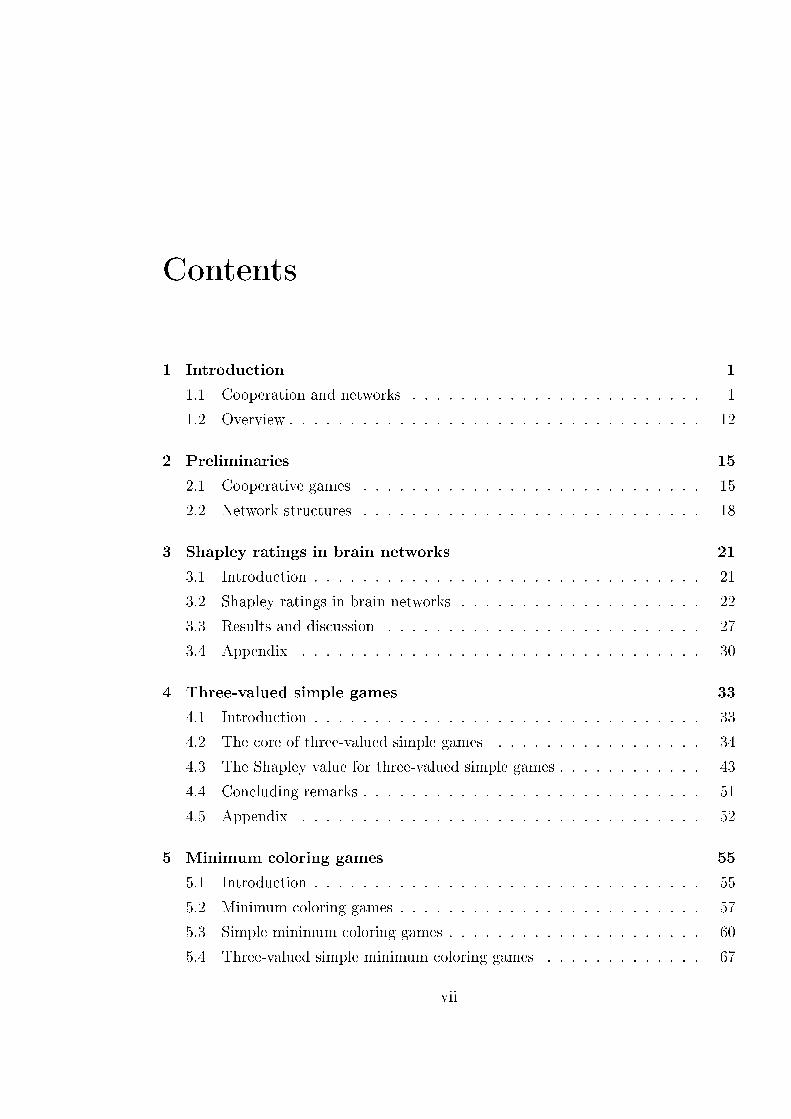
example considers a ctive brain network as a didactic illustration.
1
2
3
4
Figure 1.1: A didactic example of a brain network
1.1. Cooperation and networks 3
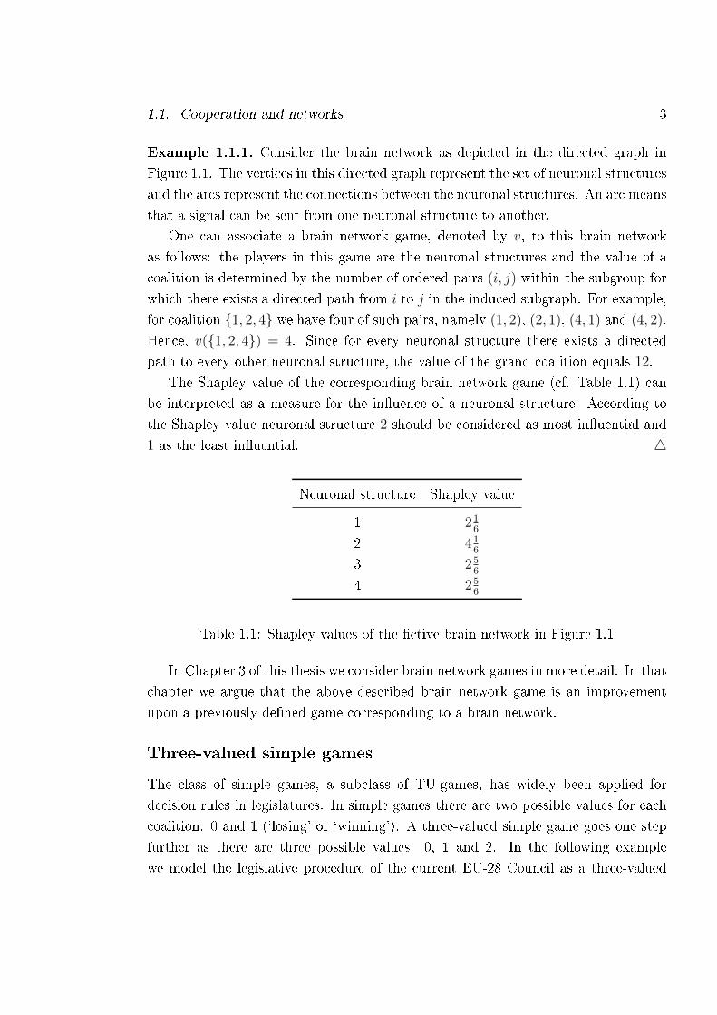
Example 1.1.1. Consider the brain network as depicted in the directed graph in
Figure 1.1. The vertices in this directed graph represent the set of neuronal structures
and the arcs represent the connections between the neuronal structures. An arc means
that a signal can be sent from one neuronal structure to another.
One can associate a brain network game, denoted by v, to this brain network
as follows: the players in this game are the neuronal structures and the value of a
coalition is determined by the number of ordered pairs (i, j) within the subgroup for
which there exists a directed path from i to j in the induced subgraph. For example,
for coalition 1, 2, 4 we have four of such pairs, namely (1, 2), (2, 1), (4, 1) and (4, 2).
Hence, v(1, 2, 4) = 4. Since for every neuronal structure there exists a directed
path to every other neuronal structure, the value of the grand coalition equals 12.
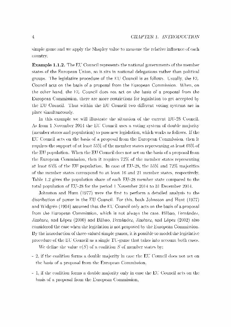
The Shapley value of the corresponding brain network game (cf. Table 1.1) can
be interpreted as a measure for the inuence of a neuronal structure. According to
the Shapley value neuronal structure 2 should be considered as most inuential and
1 as the least inuential. 4
Neuronal structure Shapley value
1 216
2 416
3 256
4 256
Table 1.1: Shapley values of the ctive brain network in Figure 1.1
In Chapter 3 of this thesis we consider brain network games in more detail. In that
chapter we argue that the above described brain network game is an improvement
upon a previously dened game corresponding to a brain network.
Three-valued simple games
The class of simple games, a subclass of TU-games, has widely been applied for
decision rules in legislatures. In simple games there are two possible values for each
coalition: 0 and 1 (`losing' or `winning'). A three-valued simple game goes one step
further as there are three possible values: 0, 1 and 2. In the following example
we model the legislative procedure of the current EU-28 Council as a three-valued
4 CHAPTER 1. INTRODUCTION
simple game and we apply the Shapley value to measure the relative inuence of each
country.
Example 1.1.2. The EU Council represents the national governments of the member
states of the European Union, so it sits in national delegations rather than political
groups. The legislative procedure of the EU Council is as follows. Usually, the EU
Council acts on the basis of a proposal from the European Commission. When, on
the other hand, the EU Council does not act on the basis of a proposal from the
European Commission, there are more restrictions for legislation to get accepted by
the EU Council. Thus within the EU Council two dierent voting systems are in
place simultaneously.
In this example we will illustrate the situation of the current EU-28 Council.
As from 1 November 2014 the EU Council uses a voting system of double majority
(member states and population) to pass new legislation, which works as follows. If the
EU Council acts on the basis of a proposal from the European Commission, then it
requires the support of at least 55% of the member states representing at least 65% of
the EU population. When the EU Council does not act on the basis of a proposal from
the European Commission, then it requires 72% of the member states representing
at least 65% of the EU population. In case of EU-28, the 55% and 72% majorities
of the member states correspond to at least 16 and 21 member states, respectively.
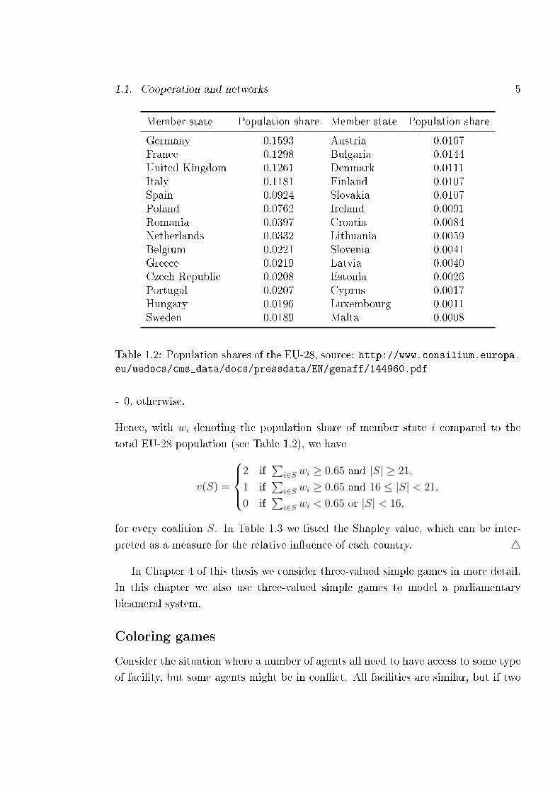
Table 1.2 gives the population share of each EU-28 member state compared to the
total population of EU-28 for the period 1 November 2014 to 31 December 2014.
Johnston and Hunt (1977) were the rst to perform a detailed analysis to the
distribution of power in the EU Council. For this, both Johnston and Hunt (1977)
and Widgrén (1994) assumed that the EU Council only acts on the basis of a proposal
from the European Commission, which is not always the case. Bilbao, Fernández,
Jiménez, and López (2000) and Bilbao, Fernández, Jiménez, and López (2002) also
considered the case when the legislation is not proposed by the European Commission.
By the introduction of three-valued simple games, it is possible to model the legislative
procedure of the EU Council as a single TU-game that takes into account both cases.
We dene the value v(S) of a coalition S of member states by:
- 2, if the coalition forms a double majority in case the EU Council does not act on
the basis of a proposal from the European Commission,
- 1, if the coalition forms a double majority only in case the EU Council acts on the
basis of a proposal from the European Commission,
1.1. Cooperation and networks 5
Member state Population share Member state Population share
Germany 0.1593 Austria 0.0167France 0.1298 Bulgaria 0.0144United Kingdom 0.1261 Denmark 0.0111Italy 0.1181 Finland 0.0107Spain 0.0924 Slovakia 0.0107Poland 0.0762 Ireland 0.0091Romania 0.0397 Croatia 0.0084Netherlands 0.0332 Lithuania 0.0059Belgium 0.0221 Slovenia 0.0041Greece 0.0219 Latvia 0.0040Czech Republic 0.0208 Estonia 0.0026Portugal 0.0207 Cyprus 0.0017Hungary 0.0196 Luxembourg 0.0011Sweden 0.0189 Malta 0.0008
Table 1.2: Population shares of the EU-28, source: http://www.consilium.europa.eu/uedocs/cms_data/docs/pressdata/EN/genaff/144960.pdf
- 0, otherwise.
Hence, with wi denoting the population share of member state i compared to the
total EU-28 population (see Table 1.2), we have
v(S) =
2 if
∑i∈S wi ≥ 0.65 and |S| ≥ 21,
1 if∑
i∈S wi ≥ 0.65 and 16 ≤ |S| < 21,
0 if∑
i∈S wi < 0.65 or |S| < 16,
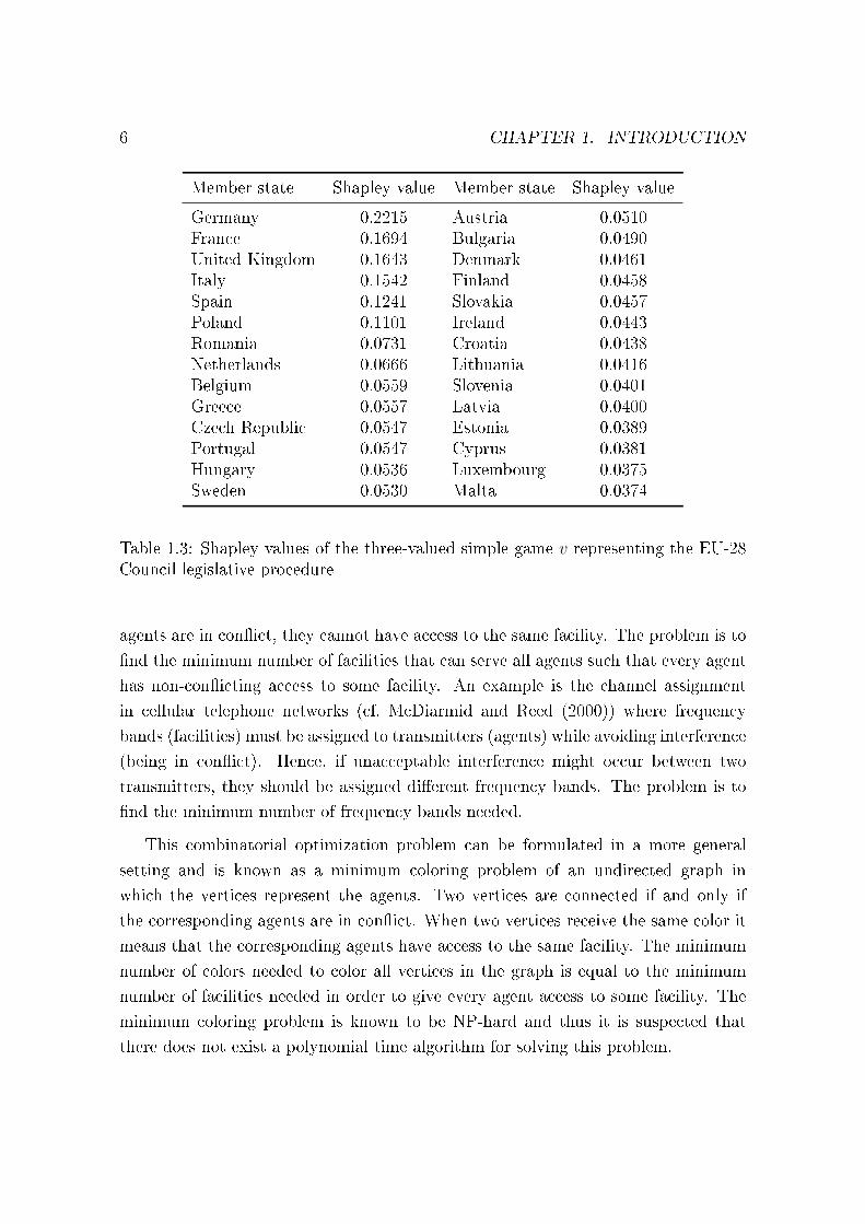
for every coalition S. In Table 1.3 we listed the Shapley value, which can be inter-
preted as a measure for the relative inuence of each country. 4
In Chapter 4 of this thesis we consider three-valued simple games in more detail.
In this chapter we also use three-valued simple games to model a parliamentary
bicameral system.
Coloring games
Consider the situation where a number of agents all need to have access to some type
of facility, but some agents might be in conict. All facilities are similar, but if two
6 CHAPTER 1. INTRODUCTION
Member state Shapley value Member state Shapley value
Germany 0.2215 Austria 0.0510France 0.1694 Bulgaria 0.0490United Kingdom 0.1643 Denmark 0.0461Italy 0.1542 Finland 0.0458Spain 0.1241 Slovakia 0.0457Poland 0.1101 Ireland 0.0443Romania 0.0731 Croatia 0.0438Netherlands 0.0666 Lithuania 0.0416Belgium 0.0559 Slovenia 0.0401Greece 0.0557 Latvia 0.0400Czech Republic 0.0547 Estonia 0.0389Portugal 0.0547 Cyprus 0.0381Hungary 0.0536 Luxembourg 0.0375Sweden 0.0530 Malta 0.0374
Table 1.3: Shapley values of the three-valued simple game v representing the EU-28Council legislative procedure
agents are in conict, they cannot have access to the same facility. The problem is to
nd the minimum number of facilities that can serve all agents such that every agent
has non-conicting access to some facility. An example is the channel assignment
in cellular telephone networks (cf. McDiarmid and Reed (2000)) where frequency
bands (facilities) must be assigned to transmitters (agents) while avoiding interference
(being in conict). Hence, if unacceptable interference might occur between two
transmitters, they should be assigned dierent frequency bands. The problem is to
nd the minimum number of frequency bands needed.
This combinatorial optimization problem can be formulated in a more general
setting and is known as a minimum coloring problem of an undirected graph in
which the vertices represent the agents. Two vertices are connected if and only if
the corresponding agents are in conict. When two vertices receive the same color it
means that the corresponding agents have access to the same facility. The minimum
number of colors needed to color all vertices in the graph is equal to the minimum
number of facilities needed in order to give every agent access to some facility. The
minimum coloring problem is known to be NP-hard and thus it is suspected that
there does not exist a polynomial time algorithm for solving this problem.
1.1. Cooperation and networks 7
The next question that arises is how to allocate the total costs among the agents,
where we assume that the total costs are linearly increasing with the number of fa-
cilities used. If there is an agent that is in conict with many other agents, then
he causes a substantial part of the total coloring costs. Therefore, it might be fair
that this agent also pays a substantial part of the total coloring costs. This issue
of allocating the total coloring costs among all players can be analyzed by the fol-
lowing cost savings TU-game: assuming that initially every agent has its individual
facility, the value of a coalition is determined by the number of colors that are saved
due to cooperation. The following numerical example shows the computation of the
corresponding TU-game.
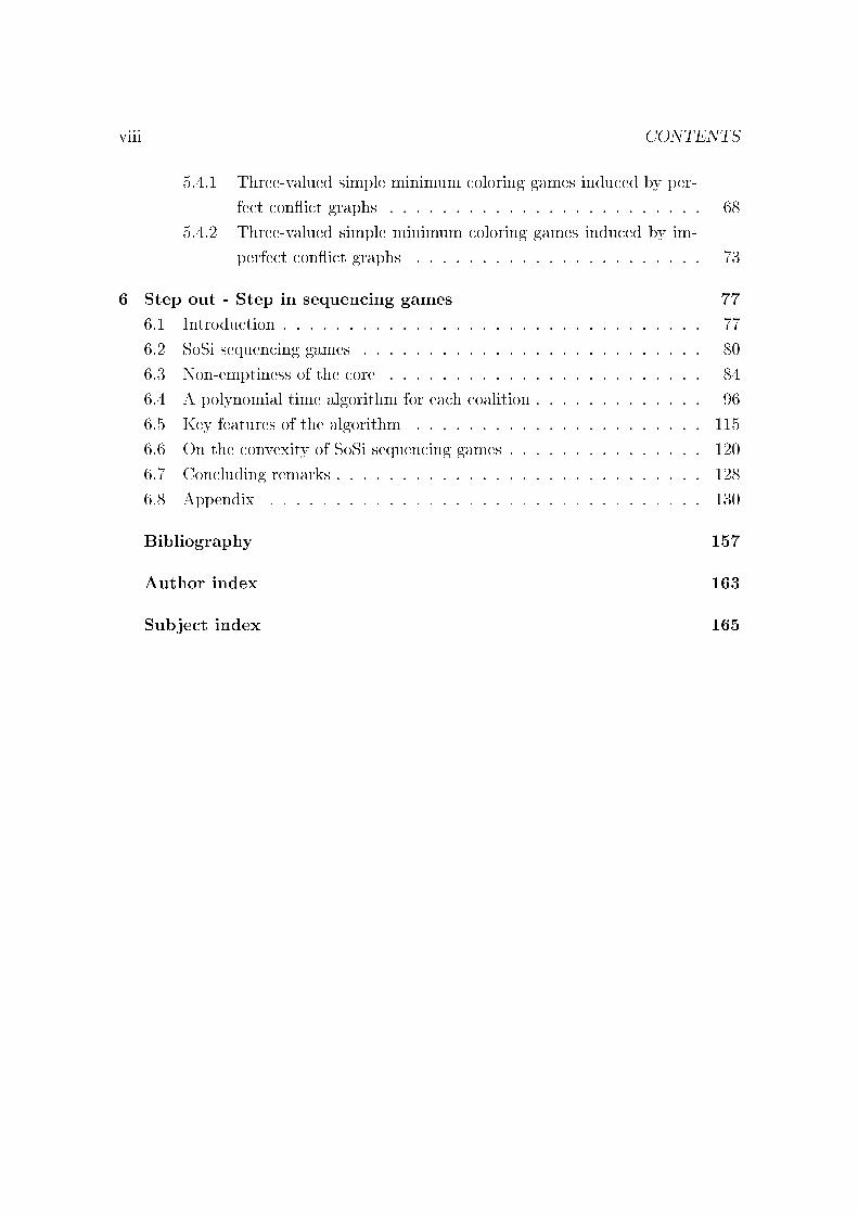
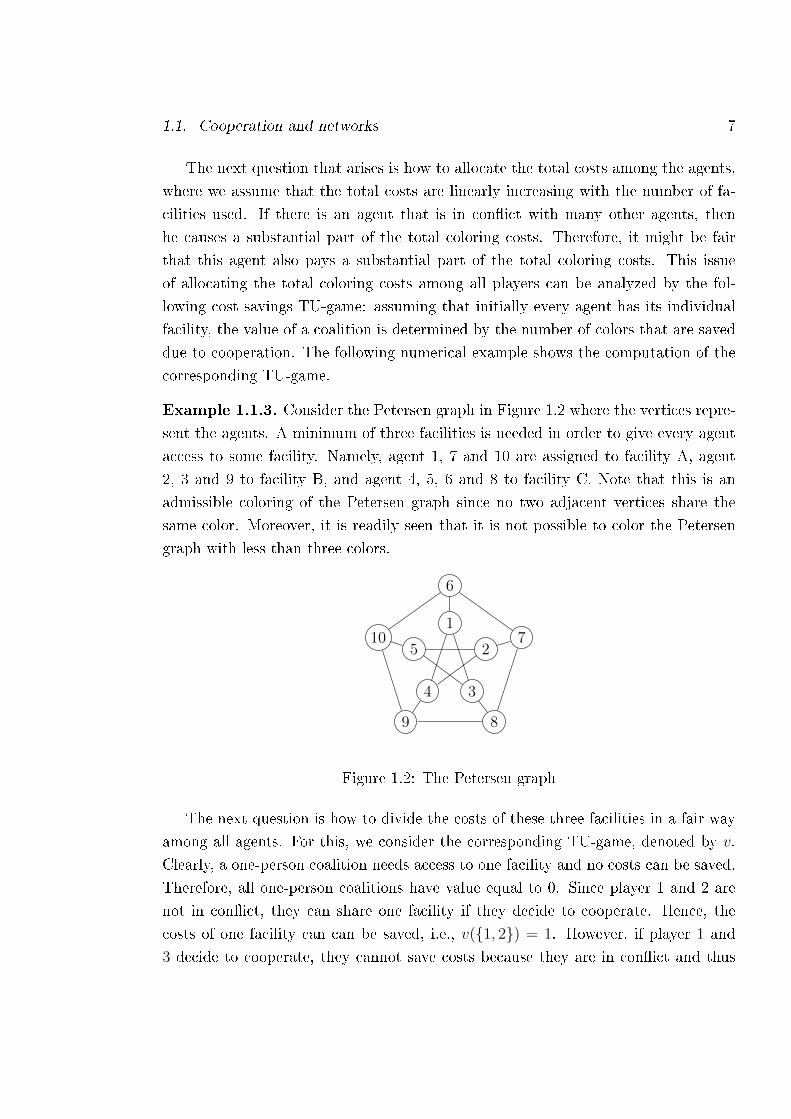
Example 1.1.3. Consider the Petersen graph in Figure 1.2 where the vertices repre-
sent the agents. A minimum of three facilities is needed in order to give every agent
access to some facility. Namely, agent 1, 7 and 10 are assigned to facility A, agent
2, 3 and 9 to facility B, and agent 4, 5, 6 and 8 to facility C. Note that this is an
admissible coloring of the Petersen graph since no two adjacent vertices share the
same color. Moreover, it is readily seen that it is not possible to color the Petersen
graph with less than three colors.
1
2
34
5
6
7
89
10
Figure 1.2: The Petersen graph
The next question is how to divide the costs of these three facilities in a fair way
among all agents. For this, we consider the corresponding TU-game, denoted by v.
Clearly, a one-person coalition needs access to one facility and no costs can be saved.
Therefore, all one-person coalitions have value equal to 0. Since player 1 and 2 are
not in conict, they can share one facility if they decide to cooperate. Hence, the
costs of one facility can can be saved, i.e., v(1, 2) = 1. However, if player 1 and
3 decide to cooperate, they cannot save costs because they are in conict and thus
8 CHAPTER 1. INTRODUCTION
v(1, 3) = 0. Moreover, if player 4, 5 and 6 decide to cooperate, they save the costs
of two facilities and thus v(4, 5, 6) = 2. 4
In Chapter 5 of this thesis we consider in particular minimum coloring problems
that lead to three-valued simple cost savings games.
Sequencing games
In a one-machine sequencing situation there are a number of jobs that have to be
processed on a single machine. The processing time of a job is the time the machine
takes to process this job. The objective in a sequencing situation is to nd a processing
order that minimizes a certain cost criterion. A widely used cost criterion is the total
weighted completion time when the individual costs are linearly increasing with the
time this job is in the system. As an example, consider a situation in which there
is one oce and a number of customers. All customers are waiting in a queue for
the handling of a personal request, e.g., trucks that are waiting at a custom house
for permission to cross the border. The handling time and the costs per time unit
because of waiting can be dierent for each customer. The problem is to nd an order
that minimizes the total waiting costs of all customers together.
In order to nd an optimal processing order, customers with high missed revenues
per time unit should be handled as early as possible. On the other hand, customers
with high handling time should be handled as late as possible, so that the waiting
time for the other customers is as low as possible. The urgency to handle a customer
is determined by the balance of these two concepts. More precisely, denote the
processing time of job i by pi. Moreover, let the costs of job i of spending t time
units in the system be given by the linear cost function ci(t) = αit with αi > 0.
Then, a processing order that minimizes the total costs is an order where the jobs are
processed in non-increasing order with respect to their urgency ui dened by ui = αipi
(cf. Smith (1956)).
Sequencing games (as introduced by Curiel, Pederzoli, and Tijs (1989)) arise from
one-machine sequencing situations by assigning a player to each job. By assuming
the presence of an initial processing order, rearranging the jobs, in order to go from
the initial processing order to an optimal processing order, will lead to cost savings.
The question is how to allocate the total cost savings among the players in a fair way.
To analyze this problem, we can study the following TU-game in which the value
of a coalition is determined by the maximal cost savings this coalition can make
1.1. Cooperation and networks 9
by means of admissible rearrangements, which (classically) ensures that the players
outside the coalition keep the same predecessors. Curiel et al. (1989) showed that
such sequencing games have a non-empty core. The following numerical example
shows the computation of the corresponding TU-game.
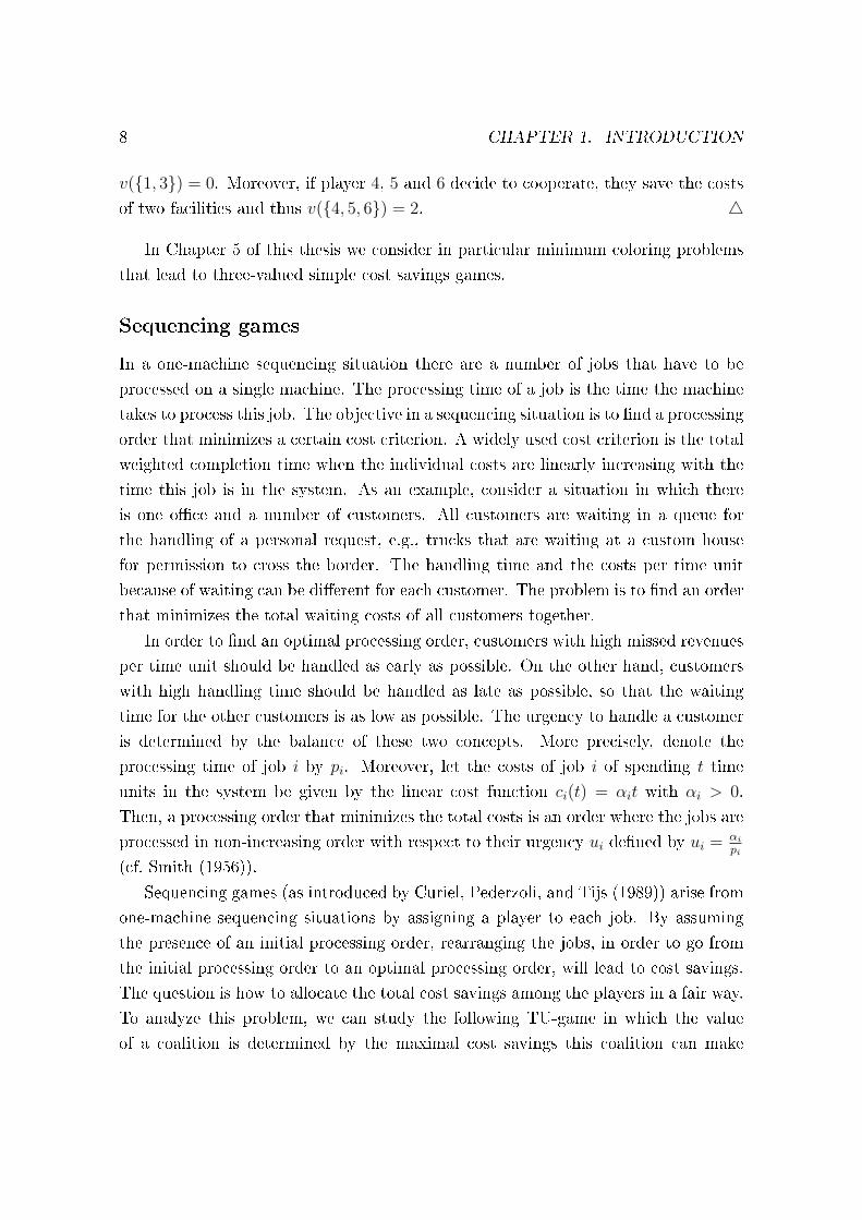
Example 1.1.4. Consider a one-machine sequencing situation with three players
denoted by 1, 2 and 3 respectively, each with one job to be processed by the single
machine, which is denoted by M. Take as initial order the order (1 2 3) (cf. Figure 1.3).
M 1 2 3
Figure 1.3: Example of a one-machine sequencing situation
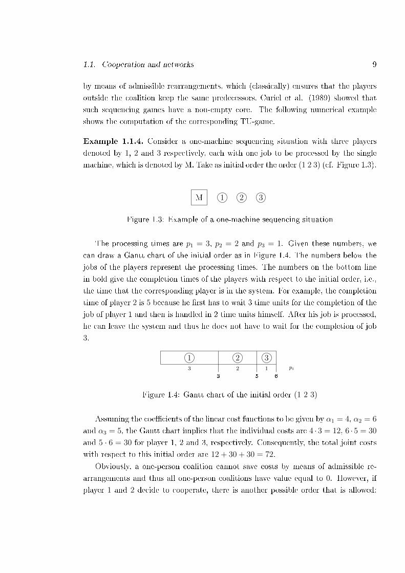
The processing times are p1 = 3, p2 = 2 and p3 = 1. Given these numbers, we
can draw a Gantt chart of the initial order as in Figure 1.4. The numbers below the
jobs of the players represent the processing times. The numbers on the bottom line
in bold give the completion times of the players with respect to the initial order, i.e.,
the time that the corresponding player is in the system. For example, the completion
time of player 2 is 5 because he rst has to wait 3 time units for the completion of the
job of player 1 and then is handled in 2 time units himself. After his job is processed,
he can leave the system and thus he does not have to wait for the completion of job
3.
1 2 33
3
2
5
1
6
pi
Figure 1.4: Gantt chart of the initial order (1 2 3)
Assuming the coecients of the linear cost functions to be given by α1 = 4, α2 = 6
and α3 = 5, the Gantt chart implies that the individual costs are 4 · 3 = 12, 6 · 5 = 30
and 5 · 6 = 30 for player 1, 2 and 3, respectively. Consequently, the total joint costs
with respect to this initial order are 12 + 30 + 30 = 72.
Obviously, a one-person coalition cannot save costs by means of admissible re-
arrangements and thus all one-person coalitions have value equal to 0. However, if
player 1 and 2 decide to cooperate, there is another possible order that is allowed:
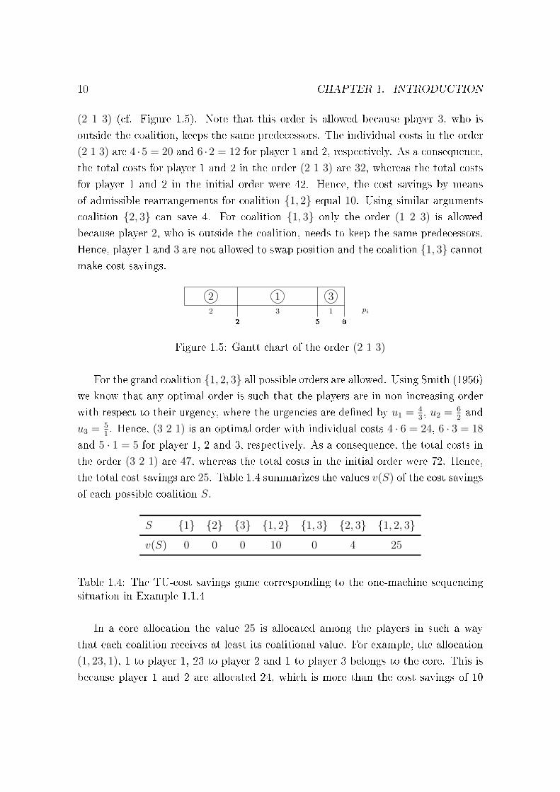
10 CHAPTER 1. INTRODUCTION
(2 1 3) (cf. Figure 1.5). Note that this order is allowed because player 3, who is
outside the coalition, keeps the same predecessors. The individual costs in the order
(2 1 3) are 4 ·5 = 20 and 6 ·2 = 12 for player 1 and 2, respectively. As a consequence,
the total costs for player 1 and 2 in the order (2 1 3) are 32, whereas the total costs
for player 1 and 2 in the initial order were 42. Hence, the cost savings by means
of admissible rearrangements for coalition 1, 2 equal 10. Using similar arguments
coalition 2, 3 can save 4. For coalition 1, 3 only the order (1 2 3) is allowed
because player 2, who is outside the coalition, needs to keep the same predecessors.
Hence, player 1 and 3 are not allowed to swap position and the coalition 1, 3 cannotmake cost savings.
2 1 32
2
3
5
1
6
pi
Figure 1.5: Gantt chart of the order (2 1 3)
For the grand coalition 1, 2, 3 all possible orders are allowed. Using Smith (1956)
we know that any optimal order is such that the players are in non-increasing order
with respect to their urgency, where the urgencies are dened by u1 = 43, u2 = 6
2and
u3 = 51. Hence, (3 2 1) is an optimal order with individual costs 4 · 6 = 24, 6 · 3 = 18
and 5 · 1 = 5 for player 1, 2 and 3, respectively. As a consequence, the total costs in
the order (3 2 1) are 47, whereas the total costs in the initial order were 72. Hence,
the total cost savings are 25. Table 1.4 summarizes the values v(S) of the cost savings
of each possible coalition S.
S 1 2 3 1, 2 1, 3 2, 3 1, 2, 3
v(S) 0 0 0 10 0 4 25
Table 1.4: The TU-cost savings game corresponding to the one-machine sequencingsituation in Example 1.1.4
In a core allocation the value 25 is allocated among the players in such a way
that each coalition receives at least its coalitional value. For example, the allocation
(1, 23, 1), 1 to player 1, 23 to player 2 and 1 to player 3 belongs to the core. This is
because player 1 and 2 are allocated 24, which is more than the cost savings of 10
1.1. Cooperation and networks 11
they can obtain on their own, and player 2 and 3 are allocated 24, which is also more
than the cost savings of 4 they can obtain on their own, 4
In Chapter 6 of this thesis we analyze in more detail a new variant of sequencing
games, so-called Step out - Step in (SoSi) sequencing games, where the set of admis-
sible orders for a coalition is modied. Now, any player is also allowed to step out
from his position in the processing order and to step in at any position later in the
processing order.
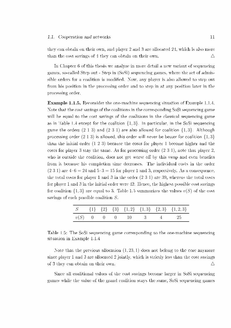
Example 1.1.5. Reconsider the one-machine sequencing situation of Example 1.1.4.
Note that the cost savings of the coalitions in the corresponding SoSi sequencing game
will be equal to the cost savings of the coalitions in the classical sequencing game
as in Table 1.4 except for the coalition 1, 3. In particular, in the SoSi sequencing
game the orders (2 1 3) and (2 3 1) are also allowed for coalition 1, 3. Although
processing order (2 1 3) is allowed, this order will never be better for coalition 1, 3than the initial order (1 2 3) because the costs for player 1 become higher and the
costs for player 3 stay the same. As for processing order (2 3 1), note that player 2,
who is outside the coalition, does not get worse o by this swap and even benets
from it because his completion time decreases. The individual costs in the order
(2 3 1) are 4 ·6 = 24 and 5 ·3 = 15 for player 1 and 3, respectively. As a consequence,
the total costs for player 1 and 3 in the order (2 3 1) are 39, whereas the total costs
for player 1 and 3 in the initial order were 42. Hence, the highest possible cost savings
for coalition 1, 3 are equal to 3. Table 1.5 summarizes the values v(S) of the cost
savings of each possible coalition S.
S 1 2 3 1, 2 1, 3 2, 3 1, 2, 3
v(S) 0 0 0 10 3 4 25
Table 1.5: The SoSi sequencing game corresponding to the one-machine sequencingsituation in Example 1.1.4
Note that the previous allocation (1, 23, 1) does not belong to the core anymore
since player 1 and 3 are allocated 2 jointly, which is strictly less than the cost savings
of 3 they can obtain on their own. 4
Since all coalitional values of the cost savings become larger in SoSi sequencing
games while the value of the grand coalition stays the same, SoSi sequencing games
12 CHAPTER 1. INTRODUCTION
might not have a non-empty core anymore. In Chapter 6 we study the core of SoSi
sequencing games and, among other things, we provide a polynomial time algorithm
determining an optimal processing order for a coalition in a SoSi sequencing game.
1.2 Overview
In Chapter 2 we introduce some general basic notions, concepts and denitions re-
garding cooperative games and network structures.
Chapter 3 considers the problem of computing the inuence of a neuronal struc-
ture in a brain network. Abraham, Kötter, Krumnack, and Wanke (2006) computed
this inuence by using the Shapley value of a coalitional game corresponding to a
directed network as a rating. Kötter, Reid, Krumnack, Wanke, and Sporns (2007)
applied this rating to large-scale brain networks, in particular to the macaque visual
cortex and the macaque prefrontal cortex. The aim of this chapter is to improve
upon the above technique by measuring the importance of subgroups of neuronal
structures in a dierent way. This new modeling technique not only leads to a more
intuitive coalitional game, but also allows for specifying the relative inuence of neu-
ronal structures and a direct extension to a setting with missing information on the
existence of certain connections.
In Chapter 4 we study a specic class of TU-games, called three-valued simple
games. These games can be considered as a natural extension of simple games. We
analyze to which extent well-known results on the core and the Shapley value for
simple games can be extended to this new setting. To describe the core of a three-
valued simple game we introduce (primary and secondary) vital players, in analogy
to veto players for simple games. The vital core, which fully depends on (primary and
secondary) vital players, is shown to be a subset of the core. Moreover, it is seen that
the transfer property of Dubey (1975) can still be used to characterize the Shapley
value for three-valued simple games. We illustrate three-valued simple games and the
corresponding Shapley value in a parliamentary bicameral system.
Chapter 5 continues with simple and three-valued simple games. Namely, we char-
acterize the class of conict graphs inducing simple or three-valued simple minimum
coloring games. We provide an upper bound on the number of maximum cliques
of conict graphs inducing such games. Moreover, a characterization of the core is
provided in terms of the underlying conict graph. In particular, in case of a perfect
conict graph the core of the corresponding three-valued simple minimum coloring
1.2. Overview 13
game equals the vital core. Finally, we study for simple minimum coloring games the
decomposition into unanimity games and derive an elegant expression for the Shapley
value.
Chapter 6 introduces a new class of relaxed sequencing games: the class of Step
out - Step in (SoSi) sequencing games. In this relaxation any player within a coalition
is allowed to step out from his position in the processing order and to step in at any
position later in the processing order. First, we show non-emptiness of the core of
SoSi sequencing games by means of a more generally applicable result. Moreover,
we provide a polynomial time algorithm to determine the value and an optimal pro-
cessing order for an arbitrary coalition in a SoSi sequencing game. This algorithm
is used to prove that SoSi sequencing games are convex. In particular, we use that
in determining an optimal processing order of a coalition S ∪ i, the algorithm can
start from the optimal processing order found for coalition S and thus all information
on this optimal processing order of S can be used.

Chapter 2
Preliminaries
2.1 Cooperative games
WithN a non-empty nite set of players, a transferable utility (TU) game is a function
v : 2N → R which assigns a number to each coalition S ∈ 2N , where 2N denotes
the collection of all subsets of N . The value v(S) in general represents the highest
joint monetary payo or cost savings the coalition S can jointly generate by means of
optimal cooperation without any help of the players inN\S. By convention, v(∅) = 0.
Let TUN denote the class of all TU-games with player set N .
A game v ∈ TUN is called monotonic if v(S) ≤ v(T ) for all S, T ∈ 2N\∅ withS ⊂ T . Hence, in a monotonic game the worth of a coalition increases when the
coalition grows. The game v is called superadditive if v(S ∪ T ) ≥ v(S) + v(T ) for
all S, T ∈ 2N\∅ with S ∩ T = ∅. Hence, in a superadditive game breaking up a
coalition into parts does not pay. It is desirable that TU-games satisfy the two basic
properties of monotonicity and superadditivity, since they provide a clear incentive for
cooperation in the grand coalition and thus provides a motivation to focus on fairly
allocating the worth of the grand coalition. Note that every nonnegative superadditive
game is monotonic. The game v is called convex (Shapley (1971)) if
v(S ∪ i)− v(S) ≤ v(T ∪ i)− v(T ), (2.1)
for all S, T ∈ 2N\∅, i ∈ N such that S ⊂ T ⊆ N\i, i.e., the incentive for joininga coalition increases as the coalition grows. Using recursive arguments it can be seen
that in order to prove convexity it is sucient to show (2.1) for the case |T | = |S|+ 1
which boils down to
v(S ∪ i)− v(S) ≤ v(S ∪ j ∪ i)− v(S ∪ j), (2.2)
15
16 CHAPTER 2. PRELIMINARIES
for all S ∈ 2N\∅, i, j ∈ N and i 6= j such that S ⊆ N\i, j.A game v ∈ TUN is called simple if
(i) v(S) ∈ 0, 1 for all S ⊂ N ,
(ii) v(N) = 1,
(iii) v is monotonic.
A coalition is winning if v(S) = 1 and losing if v(S) = 0. Let SIN denote the class of
all simple games with player set N . For v ∈ SIN the set of veto players is dened by
veto(v) =⋂S | v(S) = 1.
Hence, the veto players are those players who belong to every coalition with value 1.
An example of a simple game is a unanimity game, where for each T ∈ 2N\∅,the unanimity game uT ∈ TUN is dened by
uT (S) =
1 if T ⊆ S,
0 otherwise,
for all S ∈ 2N . Unanimity games play an important role since every game v ∈ TUN
can be written in a unique way as a linear combination of unanimity games, i.e.,
v =∑
T∈2N\∅
cTuT ,
where cT ∈ R is uniquely determined for all T ∈ 2N\∅ by the recursive formula
(cf. Harsanyi (1958))
cT = v(T )−∑
S:S⊂T,S 6=∅
cS.
The core (Gillies (1959)), C(v), of a game v ∈ TUN is dened by
C(v) =
x ∈ RN |
∑i∈N
xi = v(N),∑i∈S
xi ≥ v(S) for all S ⊂ N
.
Hence, the core consists of all possible stable allocations of v(N) for which no coalition
has an incentive to leave the grand coalition. Consequently, if the core is empty, then
2.1. Cooperative games 17
it is not possible to nd a stable allocation of v(N). From Shapley (1971) and Ichiishi
(1981) it follows that v ∈ TUN is convex if and only if
C(v) = Conv(mσ(v) | σ ∈ Π(N)), (2.3)
where Π(N) = σ : N → 1, . . . , |N | | σ is bijective is the set of all orders on N
and the marginal vector mσ(v) ∈ RN , for σ ∈ Π(N), is dened by
mσi (v) = v(j ∈ N | σ(j) ≤ σ(i))− v(j ∈ N | σ(j) < σ(i)),
for all i ∈ N . If v ∈ SIN , then the core is given by
C(v) = Conv(ei | i ∈ veto(v)),
where for S ∈ 2N\∅, the characteristic vector eS ∈ RN is dened as
eSi =
1 if i ∈ S,0 otherwise,
for all i ∈ N .
A one-point solution f on the class GN with GN ⊆ TUN is a function f : GN →RN . So, f assigns to each game v ∈ GN a unique vector f ∈ RN . A one-point
solution f on GN satises
• eciency if∑
i∈N fi(v) = v(N) for all v ∈ GN .
• symmetry if fi(v) = fj(v) for all v ∈ GN and every pair i, j ∈ N of symmetric
players in v, where players i, j ∈ N are symmetric in v if v(S∪i) = v(S∪j)for all S ⊆ N\i, j.
• the dummy property if fi(v) = v(i) for all v ∈ GN and every dummy player i ∈N in v, where player i ∈ N is a dummy player in v if v(S∪i) = v(S)+v(i)for all S ⊆ N\i.
• additivity if f(v + w) = f(v) + f(w) for all v, w ∈ GN with v + w ∈ GN .
The Shapley value (Shapley (1953)) is a one-point solution on TUN dened by
Φi(v) =1
|N |!∑
σ∈Π(N)
mσ(v), (2.4)
18 CHAPTER 2. PRELIMINARIES
for all v ∈ TUN . Alternatively, with v =∑
T∈2N\∅ cTuT , the Shapley value is given
by
Φi(v) =∑
T∈2N :i∈T
cT|T |
, (2.5)
for all i ∈ N . Shapley (1953) characterized the Shapley value as the unique one-
point solution on the class of TU-games satisfying eciency, symmetry, the dummy
property and additivity.
A solution f on GN ⊆ TUN such that for all v, w ∈ GN also maxv, w ∈ GN
and minv, w ∈ GN , satises the transfer property if for all v, w ∈ GN we have
f(maxv, w) + f(minv, w) = f(v) + f(w),
where maxv, w and minv, w are dened by (maxv, w)(S) = maxv(S), w(S)and (minv, w)(S) = minv(S), w(S), for all S ⊆ N . Dubey (1975) showed that
the combination of the axioms of eciency, symmetry, the dummy property and the
transfer property fully determines the Shapley value on the class SIN of simple games.
2.2 Network structures
An undirected graph is represented by a pair G = (N,E), where N is a set of vertices
and E ⊆ i, j | i, j ∈ N, i 6= j is a set of edges. The graph G is complete if
E = i, j | i, j ∈ N, i 6= j, that is if every two vertices are adjacent. KN denotes
the complete graph on the set N of vertices. A cycle graph Cn is a graph G = (N,E)
for which there exists a bijection f : 1, . . . , n → N such that
E = f(i), f(i+ 1) | i ∈ 1, . . . , n− 1 ∪ f(1), f(n) .
An odd cycle graph is a cycle graph Cn where n is odd.
For S ⊆ N , the induced subgraph of G by S is the graph G[S] = (S,E[S]) where
E[S] = i, j ∈ E | i, j ∈ S. The complement of G is the graph G = (N,E) where
E = i, j | i, j ∈ N, i 6= j, i, j 6∈ E. In this thesis we only consider undirected
graphs that are connected on N , i.e., every pair of vertices is linked via a sequence of
consecutive edges in E. However, note that it still might happen that some induced
subgraph G[S] is not connected on S via E[S].
A clique in G is a set S ⊆ N such that G[S] = KS. A maximum clique of G is a
clique S of the largest possible size, i.e., a clique for which |S| is maximal. The num-
ber of vertices in a maximum clique is called the clique number of G and is denoted
2.2. Network structures 19
by ω(G). We denote the set of all maximum cliques in G by Ω(G).
A directed graph is represented by a pair G = (N,A), where N is a set of vertices
and A ⊆ (i, j) | i, j ∈ N, i 6= j is a set of arcs. The transitive closure of A,
denoted by Atr, is the set of all ordered pairs (s, t) of vertices in N for which there
exists a sequence of vertices v0 = s, v1, v2, . . . , vk = t, such that (vi−1, vi) ∈ A for
all i ∈ 1, . . . , k. The graph G is called strongly connected if Atr = (i, j) | i, j ∈N, i 6= j, that is if for every two vertices i and j in N there is a directed path
from i to j and from j to i in (N,A) as described above. For S ⊆ N , the induced
subgraph of G by S is the graph G[S] = (S,A[S]) where A[S] = (i, j) ∈ A | i, j ∈ S.The induced subgraph G[S] is called a strongly connected component of G if G[S] is
strongly connected and there does not exist a T ⊆ N with S ⊂ T such that G[T ]
is strongly connected. We denote the number of strongly connected components in
graph (N,A) by SCC(N,A).

Chapter 3
Shapley ratings in brain networks
3.1 Introduction
In this chapter, based on Musegaas, Dietzenbacher, and Borm (2016), we consider
the problem of computing the inuence of a neuronal structure in a brain network.
Previously described measures for the inuence of neuronal structures are for example
the three Network Participation Indices (NPIs) as introduced by Kötter and Stephan
(2003). These NPIs, which are derived from simple graph theoretic measures, are
density (degree of interconnectedness), transmission (the ratio of outdegree to inde-
gree) and symmetry (reciprocal connectivity between a node and its neighbors). Some
other nodal connectivity measures are the clustering coecient (which measures the
connectednes of a node's neighbors, Watts and Strogatz (1998)), betweenness cen-
trality (which measures how central a node is within the network, Freeman (1977))
and dynamical importance (based on the maximum eigenvalue of the connectivity
matrix, Restrepo, Ott, and Hunt (2006)).
However, in this chapter we explore the application of cooperative game theory
in this eld. Cooperative game theory has already been used for devising centrality
measures in social networks. For example, Gómez, González-Arangüena, Manuel,
Owen, Del Pozo, and Tejada (2003) dened a centrality measure in a social net-
work as the dierence between the actor's Shapley value in the graph-restricted game
and the original game. The aim of this chapter is to improve upon the techniques
underlying the game theoretic methodology proposed by Abraham, Kötter, Krum-
nack, and Wanke (2006). Note that this chapter has a style which deviates from the
other chapters in this thesis as the main focus of this chapter is on an application of
cooperative game theory and thus not on the theory itself.
21
22 CHAPTER 3. SHAPLEY RATINGS IN BRAIN NETWORKS
Abraham et al. (2006) considered a coalitional game in which the worth of a
coalition of vertices, the neuronal structures, is dened as the number of strongly
connected components in its induced subnetwork within the whole brain network.
Subsequently, Abraham et al. (2006) computed the inuence of a neuronal structure
in a brain network by using the Shapley value of this coalitional game as a rating.
Kötter, Reid, Krumnack, Wanke, and Sporns (2007) applied this rating to large-scale
brain networks, in particular to the macaque visual cortex and the macaque prefrontal
cortex based on real-life data of Young (1992) and Walker (1940).
In this chapter we introduce an alternative coalitional game which in our opinion
has several advantages. First of all, by satisfying superadditivity the game is more
intuitive from a game theoretical point of view. Secondly, using the Shapley value
of this game as an alternative rating it allows to directly specifying relative inuence
of neuronal structures. We apply our alternative rating model to the brain networks
considered by Kötter et al. (2007) and, generally speaking, our results corroborate
the ndings of Kötter et al. (2007). Finally, a third advantage of the alternative ap-
proach is related to missing information on possible connections in a brain network.
As this feature is a common problem, as argued by Kötter and Stephan (2003), we il-
lustrate how our alternative approach allows for a direct incorporation of probabilistic
considerations regarding missing information on the existence of certain connections.
The organization of this chapter is as follows. Section 3.2 formally introduces
brain network games. In Section 3.3 we apply the Shapley rating based on the brain
network game to two large-scale brain networks. Section 3.4 consists of an appendix
with explanations about how to calculate the Shapley value for large-scale brain
networks.
3.2 Shapley ratings in brain networks
A brain network is a directed graph (N,A) where the set of vertices N represents a
set of neuronal structures and the set of arcs A represents the connections between
the neuronal structures. In this chapter we only consider strongly connected brain
networks. However, note that all analyses in this chapter are also valid in case a brain
network is not strongly connected. Abraham et al. (2006) introduced a coalitional
game (N,wA) corresponding to a brain network (N,A) dened by
wA(S) = SCC(S,A[S]),
3.2. Shapley ratings in brain networks 23
for all S ⊆ N . Hence, the worth of a coalition in wA is dened by the number of
strongly connected components (cf. Section 2.2) in its induced subgraph.
Alternatively, we dene the brain network game (N, vA) corresponding to (N,A)
by
vA(S) = |A[S]tr|,
for all S ⊆ N . Hence, the worth of a coalition S in vA is dened by the number of
ordered pairs (i, j) of vertices in S for which there exists a directed path from i to j
in (S,A[S]).
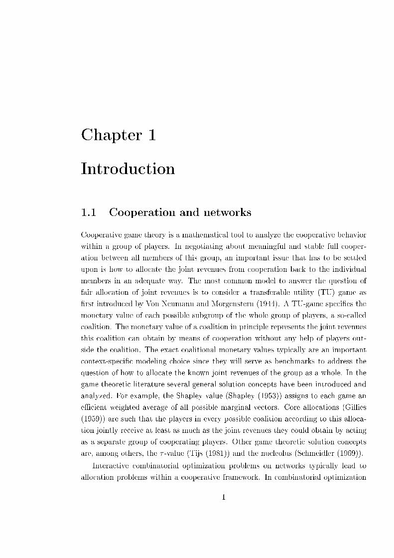
The following example shows the dierence between the games (N,wA) and (N, vA).
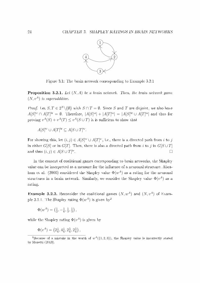
Example 3.2.1. Consider the brain network (N,A) with N = 1, 2, 3, 4 illustratedin Figure 3.1.1 Note that (N,A) is strongly connected because for every vertex in
the graph there exists a directed path to every other vertex. However, the subgraph
induced by 1, 2, 3 is not strongly connected and we have
A[1, 2, 3]tr = (1, 2), (1, 3), (2, 1), (2, 3),
and thus vA(1, 2, 3) = 4. Note that SCC(1, 2, 3, A[1, 2, 3]) = 2 because the
subgraph induced by 1, 2, 3 consists of two strongly connected components: the
subgraphs induced by 1, 2 and 3. As a consequence, wA(1, 2, 3) = 2. Table 3.1
presents the worth of every coalition in the games (N,wA) and (N, vA). Note that
(N,wA) is not superadditive since
wA(2) + wA(3, 4) = 3 > 1 = wA(2, 3, 4).
It is readily checked that (N, vA) is superadditive. 4
S i 1, 2 1, 3 1, 4 2, 3 2, 4 3, 4 1, 2, 3 1, 2, 4 1, 3, 4 2, 3, 4 N
wA(S) 1 1 2 2 2 2 2 2 2 3 1 1
vA(S) 0 2 0 0 1 1 1 4 4 1 6 12
Table 3.1: The coalitional games (N,wA) and (N, vA) corresponding to the brainnetwork in Figure 3.1
In contrast to the coalitional game (N,wA), we show in the following proposition
that the brain network game (N, vA) does satisfy superadditivity.
1This instance of a brain network is also used in Example 1 in Section 3.1 of Moretti (2013).
24 CHAPTER 3. SHAPLEY RATINGS IN BRAIN NETWORKS
1
2
3
4
Figure 3.1: The brain network corresponding to Example 3.2.1
Proposition 3.2.1. Let (N,A) be a brain network. Then, the brain network game
(N, vA) is superadditive.
Proof. Let S, T ∈ 2N\∅ with S ∩ T = ∅. Since S and T are disjoint, we also have
A[S]tr ∩ A[T ]tr = ∅. Therefore, |A[S]tr| + |A[T ]tr| = |A[S]tr ∪ A[T ]tr| and thus for
proving vA(S) + vA(T ) ≤ vA(S ∪ T ) it is sucient to show that
A[S]tr ∪ A[T ]tr ⊆ A[S ∪ T ]tr.
For showing this, let (i, j) ∈ A[S]tr ∪ A[T ]tr, i.e., there is a directed path from i to j
in either G[S] or in G[T ]. Then, there is also a directed path from i to j in G[S ∪ T ]
and thus (i, j) ∈ A[S ∪ T ]tr.
In the context of coalitional games corresponding to brain networks, the Shapley
value can be interpreted as a measure for the inuence of a neuronal structure. Abra-
ham et al. (2006) considered the Shapley value Φ(wA) as a rating for the neuronal
structures in a brain network. Similarly, we consider the Shapley value Φ(vA) as a
rating.
Example 3.2.2. Reconsider the coalitional games (N,wA) and (N, vA) of Exam-
ple 3.2.1. The Shapley rating Φ(wA) is given by2
Φ(wA) =(
12,−1
6, 1
3, 1
3
),
while the Shapley rating Φ(vA) is given by
Φ(vA) =(21
6, 41
6, 25
6, 25
6
),
2Because of a mistake in the worth of wA(1, 2, 3), the Shapley value is incorrectly statedby Moretti (2013).
3.2. Shapley ratings in brain networks 25
both determining a ranking (2, 3, 4, 1) or (2, 4, 3, 1) (there is a tie for the second highest
ranking). We note that a lower Shapley rating in wA indicates a higher inuence in
a brain network. On the contrary, a higher Shapley rating in vA indicates a higher
inuence.
Since a Shapley rating in wA can be negative, as is the case in this example, it is
not possible to determine the relative inuence of two vertices on the basis of Φ(wA).
On the other hand, a Shapley rating in vA can not be negative by denition because
(N, vA) is superadditive. Therefore, using Φ(vA), we can say that the inuence of
vertex 2 in the brain network (N,A) is almost twice as large as the inuence of vertex
1. 4
A common problem in the analysis of brain networks is the fact that it is not known
whether some specic connections (arcs) are present or not (cf. Kötter and Stephan
(2003)). Using a certain probabilistic knowledge about these unknown connections,
this lack of information can readily be incorporated in the brain network game.
We assume that each possible arc (i, j) is present with probability pij ∈ [0, 1].
Clearly, for each present arc we set pij = 1 and for each absent arc we set pij = 0. All
probabilities are summarized into a vector p. Given such a vector p, we dene the
stochastic brain network game (N, vp) in which the worth of a coalition equals the
expected (in the probabilistic sense) number of ordered pairs for which there exists
a directed path in its induced subgraph. Without providing the exact mathemat-
ical formulations the following example illustrates how to explicitly determine the
coalitional values in a stochastic brain network game.
Example 3.2.3. Reconsider the brain network presented in Example 3.2.1. Only
now suppose that the arcs (1, 4) and (4, 3) are present with probability p14 and p43,
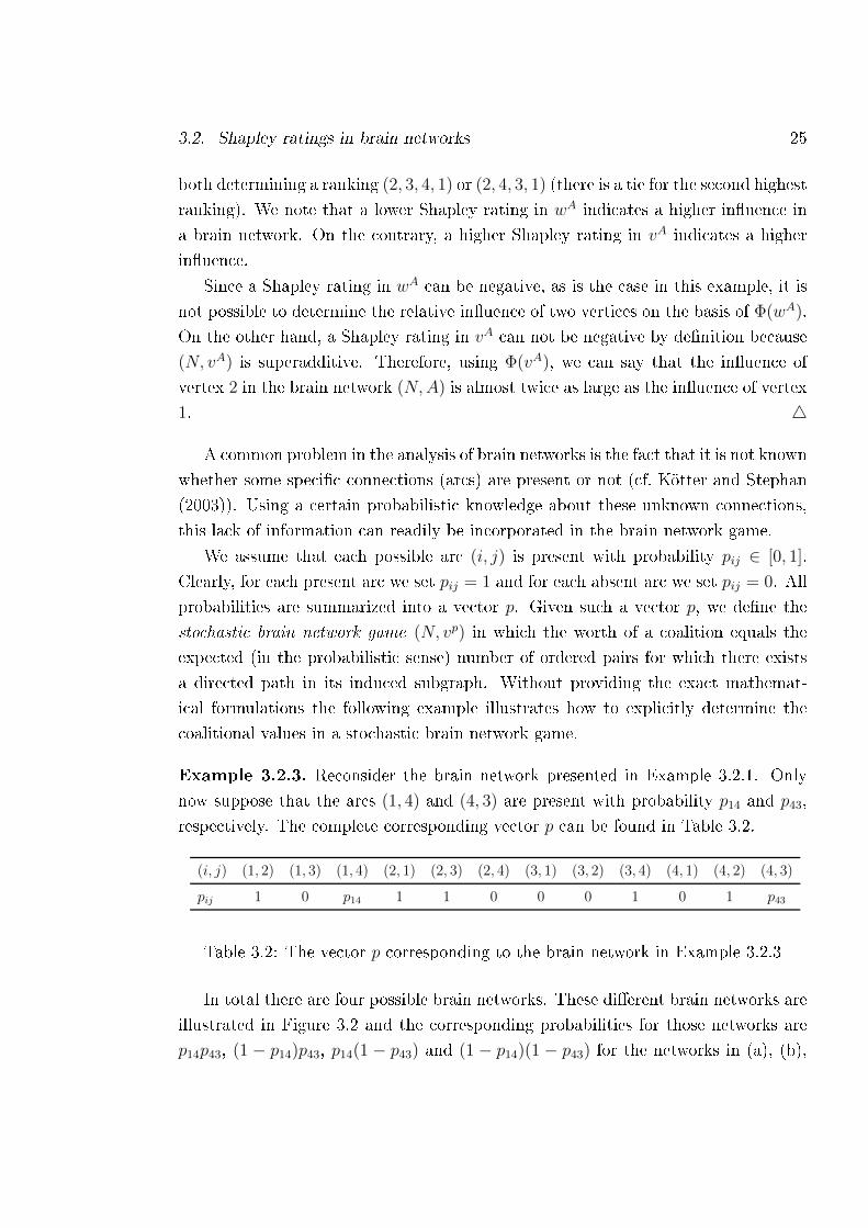
respectively. The complete corresponding vector p can be found in Table 3.2.
(i, j) (1, 2) (1, 3) (1, 4) (2, 1) (2, 3) (2, 4) (3, 1) (3, 2) (3, 4) (4, 1) (4, 2) (4, 3)
pij 1 0 p14 1 1 0 0 0 1 0 1 p43
Table 3.2: The vector p corresponding to the brain network in Example 3.2.3
In total there are four possible brain networks. These dierent brain networks are
illustrated in Figure 3.2 and the corresponding probabilities for those networks are
p14p43, (1 − p14)p43, p14(1 − p43) and (1 − p14)(1 − p43) for the networks in (a), (b),
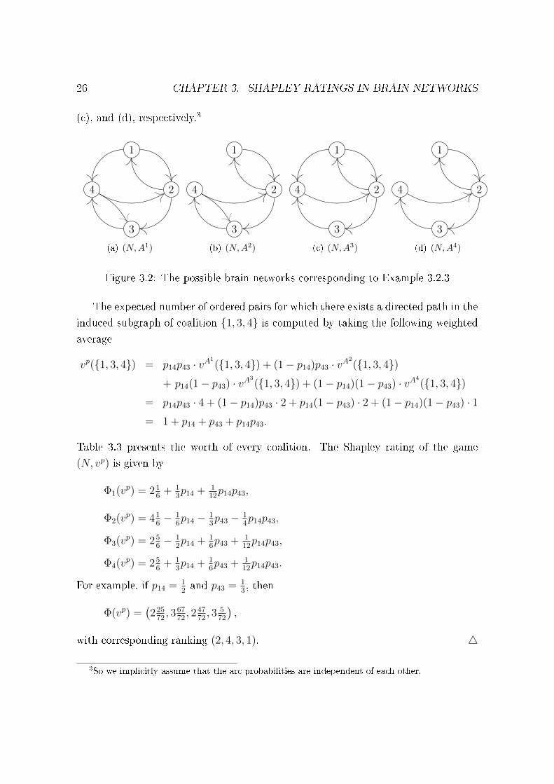
26 CHAPTER 3. SHAPLEY RATINGS IN BRAIN NETWORKS
(c), and (d), respectively.3
1
2
3
4
(a) (N,A1)
1
2
3
4
(b) (N,A2)
1
2
3
4
(c) (N,A3)
1
2
3
4
(d) (N,A4)
Figure 3.2: The possible brain networks corresponding to Example 3.2.3
The expected number of ordered pairs for which there exists a directed path in the
induced subgraph of coalition 1, 3, 4 is computed by taking the following weighted
average
vp(1, 3, 4) = p14p43 · vA1
(1, 3, 4) + (1− p14)p43 · vA2
(1, 3, 4)+ p14(1− p43) · vA3
(1, 3, 4) + (1− p14)(1− p43) · vA4
(1, 3, 4)= p14p43 · 4 + (1− p14)p43 · 2 + p14(1− p43) · 2 + (1− p14)(1− p43) · 1= 1 + p14 + p43 + p14p43.
Table 3.3 presents the worth of every coalition. The Shapley rating of the game
(N, vp) is given by
Φ1(vp) = 216
+ 13p14 + 1
12p14p43,
Φ2(vp) = 416− 1
6p14 − 1
3p43 − 1
4p14p43,
Φ3(vp) = 256− 1
2p14 + 1
6p43 + 1
12p14p43,
Φ4(vp) = 256
+ 13p14 + 1
6p43 + 1
12p14p43.
For example, if p14 = 12and p43 = 1
3, then
Φ(vp) =(225
72, 367
72, 247
72, 3 5
72
),
with corresponding ranking (2, 4, 3, 1). 4
3So we implicitly assume that the arc probabilities are independent of each other.
3.3. Results and discussion 27
S i 1, 2 1, 3 1, 4 2, 3 2, 4 3, 4 1, 2, 3 1, 2, 4 1, 3, 4 2, 3, 4 N
vp(S) 0 2 0 p14 1 1 1 + p43 4 4 + 2p14 1 + p14 + p43 + p14p43 6 12
Table 3.3: The stochastic brain network game (N, vp) corresponding to the brainnetwork in Example 3.2.3
3.3 Results and discussion
In this section we apply the Shapley rating based on the brain network game (N, vA)
to the two large-scale brain networks considered by Kötter et al. (2007) and we com-
pare the results.
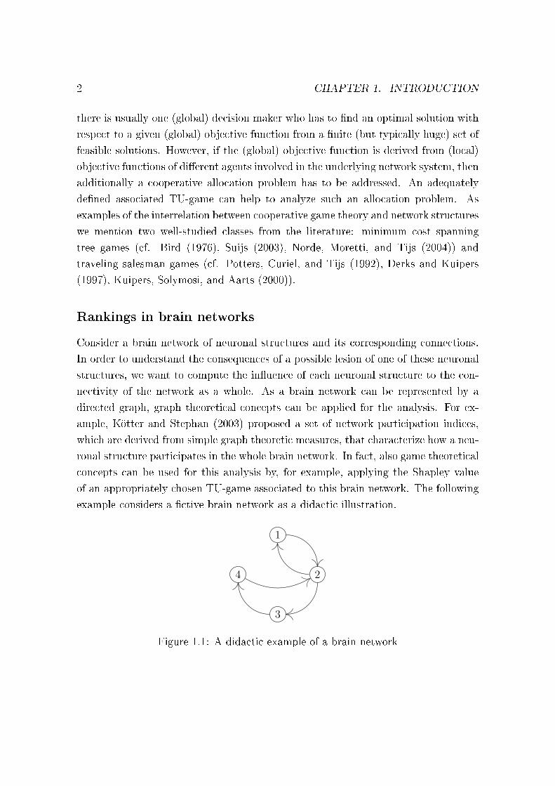
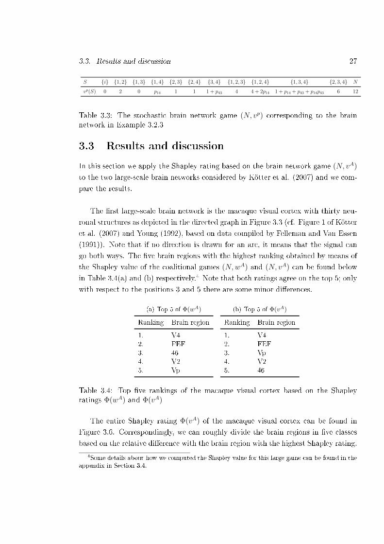
The rst large-scale brain network is the macaque visual cortex with thirty neu-
ronal structures as depicted in the directed graph in Figure 3.3 (cf. Figure 1 of Kötter
et al. (2007) and Young (1992), based on data compiled by Felleman and Van Essen
(1991)). Note that if no direction is drawn for an arc, it means that the signal can
go both ways. The ve brain regions with the highest ranking obtained by means of
the Shapley value of the coalitional games (N,wA) and (N, vA) can be found below
in Table 3.4(a) and (b) respectively.4 Note that both ratings agree on the top 5; only
with respect to the positions 3 and 5 there are some minor dierences.
(a) Top 5 of Φ(wA)
Ranking Brain region
1. V4
2. FEF
3. 46
4. V2
5. Vp
(b) Top 5 of Φ(vA)
Ranking Brain region
1. V4
2. FEF
3. Vp
4. V2
5. 46
Table 3.4: Top ve rankings of the macaque visual cortex based on the Shapleyratings Φ(wA) and Φ(vA)
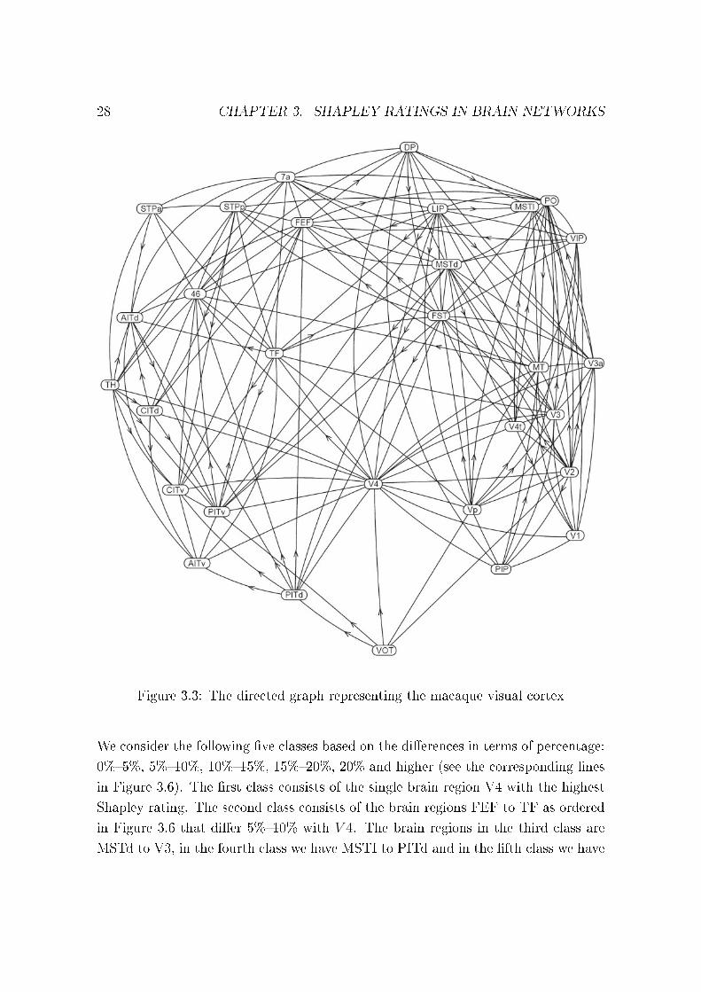
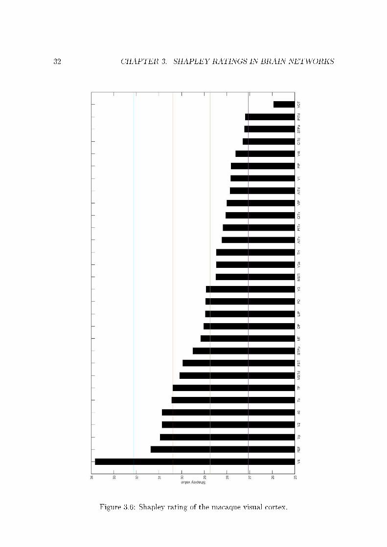
The entire Shapley rating Φ(vA) of the macaque visual cortex can be found in
Figure 3.6. Correspondingly, we can roughly divide the brain regions in ve classes
based on the relative dierence with the brain region with the highest Shapley rating.
4Some details about how we computed the Shapley value for this large game can be found in theappendix in Section 3.4.
28 CHAPTER 3. SHAPLEY RATINGS IN BRAIN NETWORKS
Figure 3.3: The directed graph representing the macaque visual cortex
We consider the following ve classes based on the dierences in terms of percentage:
0%5%, 5%10%, 10%15%, 15%20%, 20% and higher (see the corresponding lines
in Figure 3.6). The rst class consists of the single brain region V4 with the highest
Shapley rating. The second class consists of the brain regions FEF to TF as ordered
in Figure 3.6 that dier 5%10% with V 4. The brain regions in the third class are
MSTd to V3, in the fourth class we have MSTI to PITd and in the fth class we have
3.3. Results and discussion 29
the single brain region VOT with a relative inuence which is 23% lower than that
of V4.
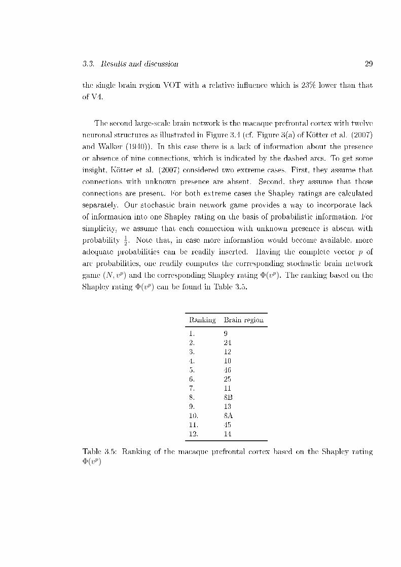
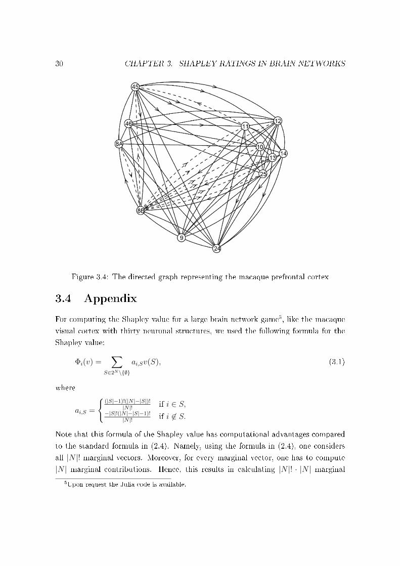
The second large-scale brain network is the macaque prefrontal cortex with twelve
neuronal structures as illustrated in Figure 3.4 (cf. Figure 3(a) of Kötter et al. (2007)
and Walker (1940)). In this case there is a lack of information about the presence
or absence of nine connections, which is indicated by the dashed arcs. To get some
insight, Kötter et al. (2007) considered two extreme cases. First, they assume that
connections with unknown presence are absent. Second, they assume that those
connections are present. For both extreme cases the Shapley ratings are calculated
separately. Our stochastic brain network game provides a way to incorporate lack
of information into one Shapley rating on the basis of probabilistic information. For
simplicity, we assume that each connection with unknown presence is absent with
probability 12. Note that, in case more information would become available, more
adequate probabilities can be readily inserted. Having the complete vector p of
arc probabilities, one readily computes the corresponding stochastic brain network
game (N, vp) and the corresponding Shapley rating Φ(vp). The ranking based on the
Shapley rating Φ(vp) can be found in Table 3.5.
Ranking Brain region
1. 9
2. 24
3. 12
4. 10
5. 46
6. 25
7. 11
8. 8B
9. 13
10. 8A
11. 45
12. 14
Table 3.5: Ranking of the macaque prefrontal cortex based on the Shapley ratingΦ(vp)
30 CHAPTER 3. SHAPLEY RATINGS IN BRAIN NETWORKS
Figure 3.4: The directed graph representing the macaque prefrontal cortex
3.4 Appendix
For computing the Shapley value for a large brain network game5, like the macaque
visual cortex with thirty neuronal structures, we used the following formula for the
Shapley value:
Φi(v) =∑
S∈2N\∅
ai,Sv(S), (3.1)
where
ai,S =
(|S|−1)!(|N |−|S|)!
|N |! if i ∈ S,−|S|!(|N |−|S|−1)!
|N |! if i 6∈ S.
Note that this formula of the Shapley value has computational advantages compared
to the standard formula in (2.4). Namely, using the formula in (2.4), one considers
all |N |! marginal vectors. Moreover, for every marginal vector, one has to compute
|N | marginal contributions. Hence, this results in calculating |N |! · |N | marginal
5Upon request the Julia code is available.
3.4. Appendix 31
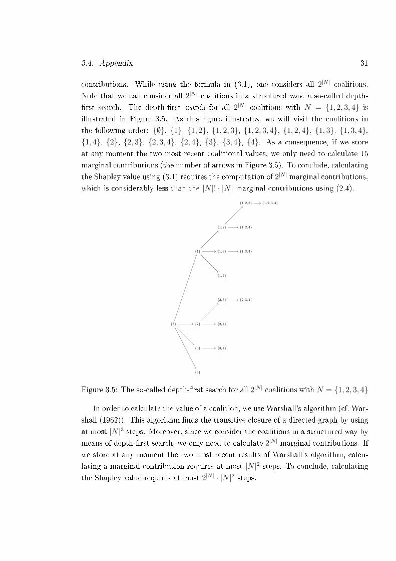
contributions. While using the formula in (3.1), one considers all 2|N | coalitions.
Note that we can consider all 2|N | coalitions in a structured way, a so-called depth-
rst search. The depth-rst search for all 2|N | coalitions with N = 1, 2, 3, 4 is
illustrated in Figure 3.5. As this gure illustrates, we will visit the coalitions in
the following order: ∅, 1, 1, 2, 1, 2, 3, 1, 2, 3, 4, 1, 2, 4, 1, 3, 1, 3, 4,1, 4, 2, 2, 3, 2, 3, 4, 2, 4, 3, 3, 4, 4. As a consequence, if we store
at any moment the two most recent coalitional values, we only need to calculate 15
marginal contributions (the number of arrows in Figure 3.5). To conclude, calculating
the Shapley value using (3.1) requires the computation of 2|N | marginal contributions,
which is considerably less than the |N |! · |N | marginal contributions using (2.4).
1
1, 2
1, 2, 3 1, 2, 3, 4
1, 2, 4
1, 3 1, 3, 4
1, 4
2
2, 3 2, 3, 4
2, 4
3 3, 4
4
∅
Figure 3.5: The so-called depth-rst search for all 2|N | coalitions with N = 1, 2, 3, 4
In order to calculate the value of a coalition, we use Warshall's algorithm (cf. War-
shall (1962)). This algorithm nds the transitive closure of a directed graph by using
at most |N |3 steps. Moreover, since we consider the coalitions in a structured way by
means of depth-rst search, we only need to calculate 2|N | marginal contributions. If
we store at any moment the two most recent results of Warshall's algorithm, calcu-
lating a marginal contribution requires at most |N |2 steps. To conclude, calculating
the Shapley value requires at most 2|N | · |N |2 steps.
32 CHAPTER 3. SHAPLEY RATINGS IN BRAIN NETWORKS
Figure 3.6: Shapley rating of the macaque visual cortex.
Chapter 4
Three-valued simple games
4.1 Introduction
In this chapter, based on Musegaas, Borm, and Quant (2015b) we analyze a class
of transferable utility games, called three-valued simple games. The class of three-
valued simple games is a natural extension of the class of simple games, introduced
by Von Neumann and Morgenstern (1944) and widely applied in the literature to
model decision rules in legislatures and other decision-making bodies. In a simple
game, a coalition is either `winning' or `losing', i.e., there are two possible values for
each coalition. The concept of three-valued simple games goes one step further than
simple games in the sense that there are three, instead of only two, possible values.
This chapter formally denes the class of three-valued simple games and focuses
on analyzing the core and the Shapley value of these games. We study how the
results for simple games can be extended to three-valued simple games. We extend
the notion of veto players in simple games, to the notion of vital players, primary
vital players and secondary vital pairs in three-valued simple games. It is known
that in simple games the core is fully determined by the veto players. In a similar
way, we introduce the vital core which fully depends on primary/secondary vital
players/pairs. The vital core is shown to be a subset of the core. We discuss a class
of three-valued simple games such that the core and the vital core coincide.
Dubey (1975) characterized the Shapley value on the class of simple games.
The essence of this characterization is the transfer property. We will show that the
transfer property can also be used for a characterization of the Shapley value for
three-valued simple games. In order to obtain this characterization we introduce
a new axiom, called unanimity level eciency. We prove that the combination of
33
34 CHAPTER 4. THREE-VALUED SIMPLE GAMES
the axioms of eciency, symmetry, the dummy property, the transfer property and
unanimity level eciency fully determines the Shapley value for a three-valued simple
game. Moreover, also the logical independence of these ve axioms is shown. At last,
as an illustration, a parliamentary bicameral system is modelled as a three-valued
simple game and analyzed on the basis of the Shapley value.
The organization of this chapter is as follows. Section 4.2 formally introduces
three-valued simple games and investigates the core of such games. Section 4.3 pro-
vides a characterization for the Shapley value on the class of three-valued simple
games. In Section 4.4 we end with some concluding remarks.
4.2 The core of three-valued simple games
In this section we dene three-valued simple games, a new subclass of TU-games.
After that, we investigate the core of such games. For this, we extend the concept
of veto players in simple games, to the concept of vital players, primary vital players
and secondary vital pairs in three-valued simple games.
A game v ∈ TUN is called three-valued simple if
(i) v(S) ∈ 0, 1, 2 for all S ⊂ N ,
(ii) v(N) = 2,
(iii) v is monotonic.
Let TSIN denote the class of all three-valued simple games with player set N . The
concept of three-valued simple games goes one step further than simple games in the
sense that there are three, instead of only two, possible values. Next to the value 0,
we have chosen the values 1 and 2. Of course, the relative proportion between these
two values may depend on the application at hand and the concept of three-valued
simple games (and its results) can be generalized to three-valued TU-games with
coalitional values 0, 1 or β with β > 1.
Recall that the core of a simple game is fully determined by its set of veto players.
We characterize the core of a three-valued simple game using the concept of vital
players which is similar to the concept of veto players in simple games. Proposi-
tion 4.2.1 below states that only the vital players of a three-valued simple game can
receive a positive payo in the core, while all other players receive zero. Here, for
4.2. The core of three-valued simple games 35
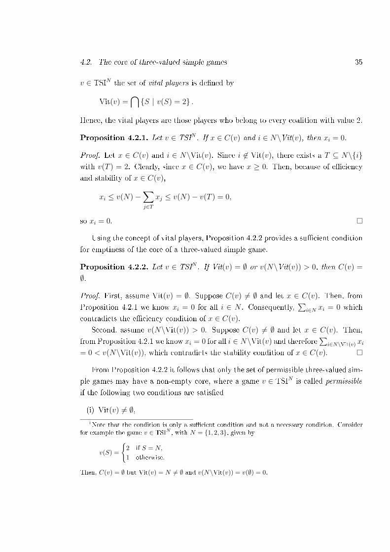
v ∈ TSIN the set of vital players is dened by
Vit(v) =⋂S | v(S) = 2 .
Hence, the vital players are those players who belong to every coalition with value 2.
Proposition 4.2.1. Let v ∈ TSIN . If x ∈ C(v) and i ∈ N\Vit(v), then xi = 0.
Proof. Let x ∈ C(v) and i ∈ N\Vit(v). Since i 6∈ Vit(v), there exists a T ⊆ N\iwith v(T ) = 2. Clearly, since x ∈ C(v), we have x ≥ 0. Then, because of eciency
and stability of x ∈ C(v),
xi ≤ v(N)−∑j∈T
xj ≤ v(N)− v(T ) = 0,
so xi = 0.
Using the concept of vital players, Proposition 4.2.2 provides a sucient condition
for emptiness of the core of a three-valued simple game.
Proposition 4.2.2. Let v ∈ TSIN . If Vit(v) = ∅ or v(N\Vit(v)) > 0, then C(v) =
∅.1
Proof. First, assume Vit(v) = ∅. Suppose C(v) 6= ∅ and let x ∈ C(v). Then, from
Proposition 4.2.1 we know xi = 0 for all i ∈ N . Consequently,∑
i∈N xi = 0 which
contradicts the eciency condition of x ∈ C(v).
Second, assume v(N\Vit(v)) > 0. Suppose C(v) 6= ∅ and let x ∈ C(v). Then,
from Proposition 4.2.1 we know xi = 0 for all i ∈ N\Vit(v) and therefore∑
i∈N\Vit(v) xi
= 0 < v(N\Vit(v)), which contradicts the stability condition of x ∈ C(v).
From Proposition 4.2.2 it follows that only the set of permissible three-valued sim-
ple games may have a non-empty core, where a game v ∈ TSIN is called permissible
if the following two conditions are satised
(i) Vit(v) 6= ∅,1Note that the condition is only a sucient condition and not a necessary condition. Consider
for example the game v ∈ TSIN , with N = 1, 2, 3, given by
v(S) =
2 if S = N,
1 otherwise.
Then, C(v) = ∅ but Vit(v) = N 6= ∅ and v(N\Vit(v)) = v(∅) = 0.
36 CHAPTER 4. THREE-VALUED SIMPLE GAMES
(ii) v(N\Vit(v)) = 0.
However, note that a permissible three-valued simple game can still have an empty
core. From now on we focus only on the set of permissible three-valued simple games
and dene for every permissible three-valued simple game, a reduced game where the
player set is reduced to the set of vital players. We dene this reduced game in such
a way that the core of a permissible three-valued simple game equals the core of the
reduced game, when extended with zeros for all players outside the set of vital players
(see Proposition 4.2.4).
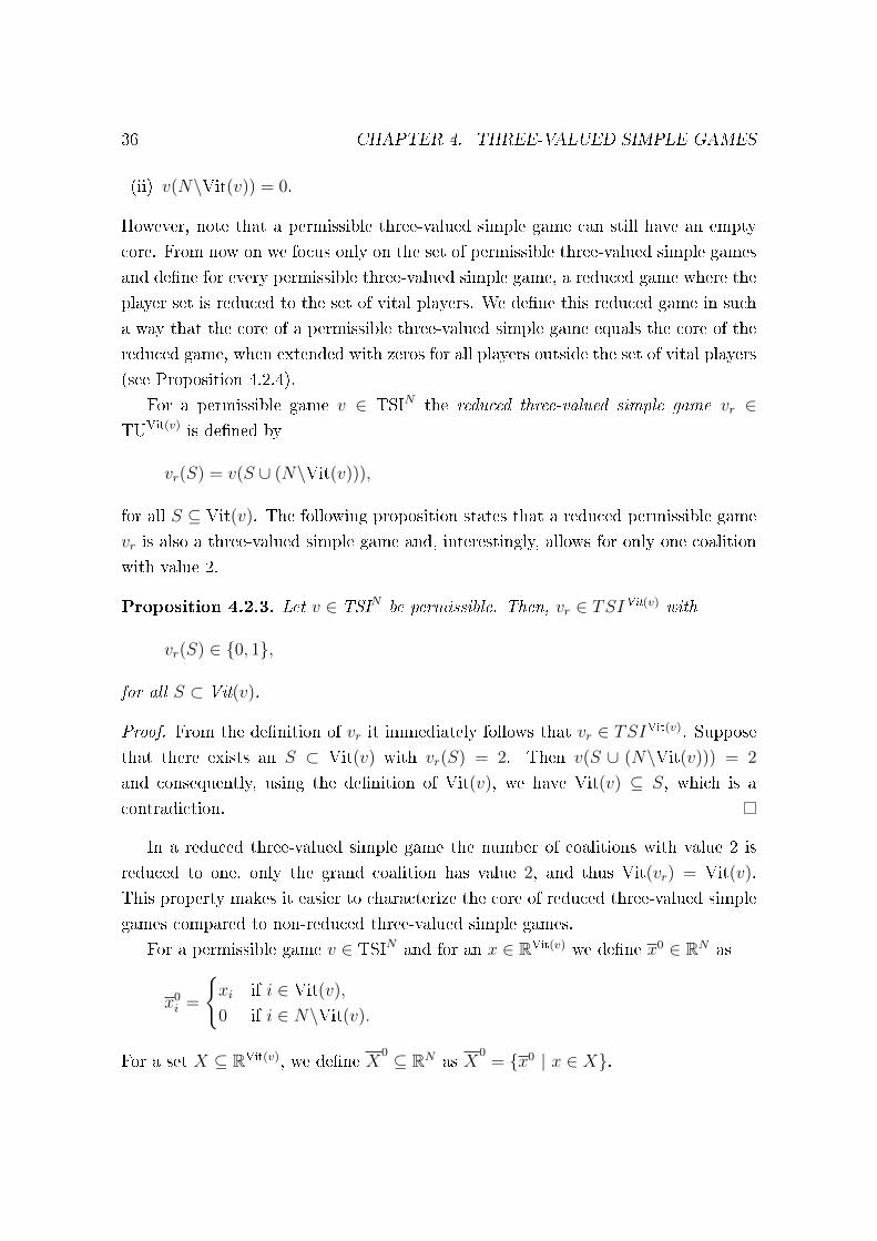
For a permissible game v ∈ TSIN the reduced three-valued simple game vr ∈TUVit(v) is dened by
vr(S) = v(S ∪ (N\Vit(v))),
for all S ⊆ Vit(v). The following proposition states that a reduced permissible game
vr is also a three-valued simple game and, interestingly, allows for only one coalition
with value 2.
Proposition 4.2.3. Let v ∈ TSIN be permissible. Then, vr ∈ TSIVit(v) with
vr(S) ∈ 0, 1,
for all S ⊂ Vit(v).
Proof. From the denition of vr it immediately follows that vr ∈ TSIVit(v). Suppose
that there exists an S ⊂ Vit(v) with vr(S) = 2. Then v(S ∪ (N\Vit(v))) = 2
and consequently, using the denition of Vit(v), we have Vit(v) ⊆ S, which is a
contradiction.
In a reduced three-valued simple game the number of coalitions with value 2 is
reduced to one, only the grand coalition has value 2, and thus Vit(vr) = Vit(v).
This property makes it easier to characterize the core of reduced three-valued simple
games compared to non-reduced three-valued simple games.
For a permissible game v ∈ TSIN and for an x ∈ RVit(v) we dene x0 ∈ RN as
x0i =
xi if i ∈ Vit(v),
0 if i ∈ N\Vit(v).
For a set X ⊆ RVit(v), we dene X0 ⊆ RN as X
0= x0 | x ∈ X.
4.2. The core of three-valued simple games 37
Proposition 4.2.4. Let v ∈ TSIN be permissible. Then,
C(v) = C(vr)0
Proof. (⊆) Let x ∈ C(v) and let S ⊆ Vit(v). From Proposition 4.2.1 we have∑i∈S
xi =∑
i∈S∪(N\Vit(v))
xi ≥ v(S ∪ (N\Vit(v))) = vr(S),
where the inequality follows from stability of x ∈ C(v). Because of eciency of
x ∈ C(v) and due to Proposition 4.2.1 we have∑i∈Vit(v)
xi =∑i∈N
xi = v(N) = 2 = vr(Vit(v)),
where the last equality follows from Proposition 4.2.3. Hence, x ∈ C(vr)0.
(⊇) Let x ∈ C(vr)0and let S ⊆ N . Then,∑
i∈S
xi =∑
i∈S∩Vit(v)
xi ≥ vr(S ∩ Vit(v)) = v((S ∩ Vit(v)) ∪ (N\Vit(v))) ≥ v(S),
where the rst inequality follows from stability of x ∈ C(vr) and the second inequality
follows from monotonicity of v and the fact that S ⊆ (S ∩ Vit(v)) ∪ (N\Vit(v)).
Because of eciency of x ∈ C(vr) we have∑i∈N
xi =∑
i∈Vit(v)
xi = vr(Vit(v)) = 2 = v(N),
where the penultimate equality follows from Proposition 4.2.3. Hence, x ∈ C(v).
Proposition 4.2.4 states that the core of a permissible three-valued simple game
follows from the core of the corresponding reduced game by extending the vectors
with zeros for the non-vital players. This proposition also implies that the core of a
permissible three-valued simple game is non-empty if and only if the corresponding
reduced game has a non-empty core. Proposition 4.2.4 is illustrated in the following
example.
Example 4.2.1. Let N = 1, 2, 3, 4 and consider the game v ∈ TSIN given by
v(S) =
2 if S ∈ 1, 2, 3, N,1 if S ∈ 1, 2, 2, 3, 1, 2, 4, 2, 3, 4,0 otherwise.
38 CHAPTER 4. THREE-VALUED SIMPLE GAMES
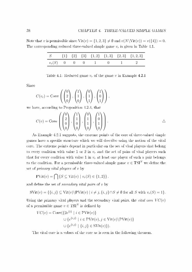
Note that v is permissible since Vit(v) = 1, 2, 3 6= ∅ and v(N\Vit(v)) = v(4) = 0.
The corresponding reduced three-valued simple game vr is given in Table 4.1.
S 1 2 3 1, 2 1, 3 2, 3 1, 2, 3
vr(S) 0 0 0 1 0 1 2
Table 4.1: Reduced game vr of the game v in Example 4.2.1
Since
C(vr) = Conv
020
,
110
,
011
,
101
,
we have, according to Proposition 4.2.4, that
C(v) = Conv
0200
,
1100
,
0110
,
1010
. 4
As Example 4.2.1 suggests, the extreme points of the core of three-valued simple
games have a specic structure which we will describe using the notion of the vital
core. The extreme points depend in particular on the set of vital players that belong
to every coalition with value 1 or 2 in vr and the set of pairs of vital players such
that for every coalition with value 1 in vr at least one player of such a pair belongs
to the coalition. For a permissible three-valued simple game v ∈ TSIN we dene the
set of primary vital players of v by
PVit(v) =⋂S ⊆ Vit(v) | vr(S) ∈ 1, 2 .
and dene the set of secondary vital pairs of v by
SVit(v) = i, j ⊆ Vit(v)\PVit(v) | i 6= j, i, j∩S 6= ∅ for all S with vr(S) = 1.
Using the primary vital players and the secondary vital pairs, the vital core V C(v)
of a permissible game v ∈ TSIN is dened by
V C(v) = Conv(2ei | i ∈ PVit(v)∪ ei,j | i ∈ PVit(v), j ∈ Vit(v)\PVit(v)∪ ei,j | i, j ∈ SVit(v)).
The vital core is a subset of the core as is seen in the following theorem.
4.2. The core of three-valued simple games 39
Theorem 4.2.5. Let v ∈ TSIN be permissible. Then,
V C(v) ⊆ C(v).
Proof. Due to Proposition 4.2.4 together with the fact that C(v) is a convex set,
it is sucient to show that 2ei ∈ C(vr) for all i ∈ PVit(v), ei,j ∈ C(vr) for all
i ∈ PVit(v) and j ∈ Vit(v)\PVit(v), and ei,j ∈ C(vr) for all i, j ∈ SVit(v).2
Let i ∈ PVit(v) and S ⊂ Vit(v). If i ∈ S, then∑k∈S
2eik = 2 > 1 ≥ vr(S).
If i 6∈ S, then vr(S) = 0 and∑k∈S
2eik = 0 = vr(S).
Moreover,∑
k∈Vit(v) 2eik = 2 = vr(Vit(v)). Hence, 2ei belongs to C(vr).
Next, let i ∈ PVit(v), j ∈ Vit(v)\PVit(v) and S ⊂ Vit(v). If i ∈ S, then∑k∈S
ei,jk ≥ 1 ≥ vr(S).
If i 6∈ S, then vr(S) = 0 and∑k∈S
ei,jk ≥ 0 = vr(S).
Moreover,∑
k∈Vit(v) ei,jk = 2 = vr(Vit(v)). Hence, ei,j belongs to C(vr).
Finally, let i, j ∈ SVit(v) and let S ⊂ Vit(v). If S ∩ i, j 6= ∅, then∑k∈S
ei,jk ≥ 1 ≥ vr(S).
If S ∩ i, j = ∅, then vr(S) = 0 and∑k∈S
ei,jk = 0 = vr(S).
Moreover,∑
k∈Vit(v) ei,jk = 2 = vr(Vit(v)). Hence, ei,j belongs to C(vr).
2By the nature of the restricted game vr we should actually write 2ei|Vit(v) and ei,j|Vit(v)
since we consider the restriction of the vectors 2ei and ei,j to Vit(v).
40 CHAPTER 4. THREE-VALUED SIMPLE GAMES
The following example illustrates that there are three-valued simple games for
which the vital core is empty, but the core is non-empty.
Example 4.2.2. Let N = 1, 2, 3, 4 and consider the game v ∈ TSIN given by
v(S) =
2 if |S| = 4,
1 if |S| = 2 or |S| = 3,
0 otherwise.
Note that Vit(v) = N , so v is permissible and the corresponding reduced three-valued
simple game vr is the same as v. Since vr(1, 2) = 1 and vr(3, 4) = 1, we have
PVit(v) = ∅. Moreover, for i, j ∈ N with i 6= j, we have vr(N\i, j) = 1. Hence,
also SVit(v) = ∅ and consequently V C(v) = ∅. However, the core of v is non-empty
since(
12, 1
2, 1
2, 1
2
)∈ C(v). 4
As the following example shows, the vital core and the core coincide for some
three-valued simple games.
Example 4.2.3. Reconsider the three-valued simple game of Example 4.2.1. From
the reduced game vr (see Table 4.1) it follows that
PVit(v) = 2
and
SVit(v) = 1, 3 .
Therefore, the vital core of v is given by
V C(v) = Conv
0200
,
1100
,
0110
,
1010
,
and, using the results from Example 4.2.1, we have V C(v) = C(V ). 4
Theorem 4.2.6 below shows that the core and the vital core coincide for the class
of double unanimity games, a specic subclass of three-valued simple games. For
T1, T2 ∈ 2N\∅, we dene the double unanimity game uT1,T2 ∈ TSIN by
uT1,T2(S) =
2 if T1 ⊆ S and T2 ⊆ S,
1 if T1 ⊆ S, T2 6⊆ S or T1 6⊆ S, T2 ⊆ S,
0 otherwise,
4.2. The core of three-valued simple games 41
for all S ∈ 2N . Note that a three-value simple double unanimity game is a natural
extension of a simple unanimity game.
Theorem 4.2.6. Let v ∈ TSIN be a double unanimity game. Then,
C(v) = V C(v).
Proof. Let T1, T2 ∈ 2N\∅ be such that v = uT1,T2 (with player set N). Observe
that the reduced three-valued simple game vr ∈ TSIT1∪T2 can also be expressed by
vr = uT1,T2 (with player set T1 ∪ T2). Therefore, the set of primary vital players of v
is given by
PVit(v) =
T1 if T1 ⊆ T2,
T2 if T2 ⊆ T1,
T1 ∩ T2 otherwise,
= T1 ∩ T2.
The set of secondary vital pairs of v is given by
SVit(v) =
∅ if T1 ⊆ T2 or T2 ⊆ T1,
i, j ⊆ T1 ∪ T2 | i ∈ T1\T2, j ∈ T2\T1 otherwise,
= i, j ⊆ T1 ∪ T2 | i ∈ T1\T2, j ∈ T2\T1.
Consequently,
V C(v) = Conv(2ei | i ∈ T1 ∩ T2∪ ei,j | i ∈ T1 ∩ T2, j ∈ T1\T2 or j ∈ T2\T1∪ ei,j | i ∈ T1\T2, j ∈ T2\T1),
From Theorem 4.2.5 we already know that V C(v) ⊆ C(v), so we only need to prove
C(v) ⊆ V C(v). Since a double unanimity game is convex, (2.3) implies that it suces
to show that
mσ(v) ∈ 2ei | i ∈ T1 ∩ T2 ∪ ei,j | i ∈ T1 ∩ T2, j ∈ T1\T2 or j ∈ T2\T1∪ ei,j | i ∈ T1\T2, j ∈ T2\T1),
for all σ ∈ Π(N).
Let σ ∈ Π(N). Since v(S) ∈ 0, 1, 2 for all S ⊆ N and v is monotonic, mσ(v)
either contains one two with all other coordinates zero (case 1) or it contains two ones
with all other coordinates zero (case 2). We thus distinguish between these two cases.
42 CHAPTER 4. THREE-VALUED SIMPLE GAMES
Case 1: mσ(v) = 2ei for some i ∈ N . Set
P = k ∈ N | σ(k) < σ(i).
Then v(P ) = 0 implying that T1 6⊆ P and T2 6⊆ P . Moreover, v(P ∪ i) = 2 and
therefore T1 ⊆ P ∪ i and T2 ⊆ P ∪ i. This is only possible if i ∈ T1 ∩ T2, conse-
quently mσ(v) = 2ei with i ∈ T1 ∩ T2.
Case 2: mσ(v) = ei,j for some i, j ∈ N , i 6= j. Without loss of generality assume
that σ(i) < σ(j). Set
P = k ∈ N | σ(k) < σ(i)
and
Q = k ∈ N | σ(k) < σ(j).
Since v(P ∪ i) = 1, assume without loss of generality that T1 ⊆ P ∪ i and
T2 6⊆ P ∪ i. Since v(P ) = 0 we have T1 6⊆ P and T2 6⊆ P . From this together with
T1 ⊆ P ∪ i it can be concluded that i ∈ T1, and thus i ∈ T1 ∩ T2 or i ∈ T1\T2.
Since v(Q) = 1 and v(Q ∪ j) = 2, it can be concluded that T1 ⊆ Q, T2 6⊆ Q and
T2 ⊆ Q ∪ j. This is only possible if j ∈ T2\T1, consequently mσ(v) = ei,j with
i ∈ T1 ∩ T2 or i ∈ T1\T2 and j ∈ T2\T1.
In Chapter 5 we discuss another class of three-valued simple games such that the
core and the vital core coincide. Example 4.2.4 illustrates that there exist three-
valued simple games for which the vital core is a strict non-empty subset of the
core.
Example 4.2.4. Let v ∈ TSIN be given by N = 1, . . . , 7 and
v(S) =
2 if S ∈ N\6, N\7, N,1 if S 6∈ N\6, N\7, N and 1, 3, 5 ⊆ S or 3, 4, 5 ⊆ S or
1, 2, 3, 6 ⊆ S or 1, 3, 4, 7 ⊆ S or 2, 3, 4, 6, 7 ⊆ S,
0 otherwise.
4.3. The Shapley value for three-valued simple games 43
Note that v is permissible since Vit(v) = 1, 2, 3, 4, 5 6= ∅ and v(N\Vit(v)) =
v(6, 7) = 0. Hence, vr ∈ TSIVit(v) is given by
vr(S) =
2 if S = Vit(v),
1 if S ∈ 1, 2, 3, 1, 3, 4, 1, 3, 5, 2, 3, 4, 3, 4, 5,1, 2, 3, 4, 1, 2, 3, 5, 1, 3, 4, 5, 2, 3, 4, 5,
0 otherwise.
From this it follows that
PVit(v) = 3
and
SVit(v) = 1, 4 .
Consequently,
V C(v) = Conv
0020000
,
1010000
,
0110000
,
0011000
,
0010100
,
1001000
.
Note that(0, 1
2, 1
2, 1
2, 1
2, 0, 0
)belongs to C(v), but does not belong to V C(v) and thus
V C(v) ⊂ C(v). 4
4.3 The Shapley value for three-valued simple games
In this section we analyze the Shapley value for three-valued simple games. In the
context of simple games and three-valued simple games, a one-point solution concept
like the Shapley value can be interpreted as a measure for the relative inuence of
each player.
A characterization of the Shapley value for simple games is provided by Dubey
(1975). The essence of this characterization is the transfer property. Dubey (1975)
proved that the unique one-point solution concept on SIN that satises eciency, sym-
metry, the dummy property and the transfer property is the Shapley value (Shapley

44 CHAPTER 4. THREE-VALUED SIMPLE GAMES
and Shubik (1954)). The aim of this section is to see if the transfer property can also
be used for a characterization for three-valued simple games.
The combination of the four properties eciency, symmetry, dummy property
and transfer property3 is not sucient to characterize the Shapley value on the class
of three-valued simple games: see Example 4.5.1 in the appendix in Section 4.5.
To obtain a characterization of Φ on TSIN , we introduce an additional fth axiom:
unanimity level eciency.
A one-point solution concept f : TSIN → RN satises unanimity level eciency
if ∑i∈S
fi(uS,T ) = 1 +1
2
∑i∈S
fi(uT,T ), (4.1)
for all S, T ∈ 2N\∅ with S ⊂ T . Unanimity level eciency intuitively states that
in a double unanimity game uS,T with S ⊂ T the players in S can allocate a payo
of 1 between themselves, while for the remaining payo of 1 (assuming eciency) the
players in S and T\S are treated equally. Formally, the unanimity level eciency
axiom compares the aggregate payo of coalition S within a double unanimity game
uS,T , with S ⊂ T , to half of the payos to S in the double unanimity game uT,T .
Note that the double unanimity game uT,T is a rescaling of the unanimity game uT
and half of the payos to S in the double unanimity game uT,T equals the payos to
S in the unanimity game uT .
The combination of the axioms of eciency, symmetry, the dummy property, the
transfer property and unanimity level eciency fully determines the Shapley value
for a three-valued simple game.
Theorem 4.3.1. The Shapley value Φ is the unique one-point solution concept on
TSIN satisfying the axioms eciency, symmetry, the dummy property, the transfer
property and unanimity level eciency.4
Proof. 5 We rst prove that, on TSIN , the Shapley value Φ satises the ve axioms
mentioned in the theorem. From Shapley (1953) it follows that Φ satises eciency,
symmetry and the dummy property on TUN . Moreover, from Dubey (1975) it follows
that Φ satises the transfer property on TUN . Hence, Φ also satises eciency,
3 If v, w ∈ TSIN , then both maxv, w and minv, w belong to TSIN too.4A proof of the logical independence of the ve axioms for |N | = 2 can be found in the appendix
in Section 4.5.5The proof is similar to the proof of Theorem II in Dubey (1975).
4.3. The Shapley value for three-valued simple games 45
symmetry, the dummy property and the transfer property on TSIN , and thus it only
remains to prove that Φ satises unanimity level eciency on TSIN . Note that, for
S, T ∈ 2N with S ⊂ T , we have
Φi(uS,T ) =
1|S| + 1
|T | if i ∈ S1|T | if i ∈ T\S,0 otherwise,
and
Φi(uT,T ) =
2|T | if i ∈ T0 otherwise,
for all i ∈ N . Consequently,∑i∈S
fi(uS,T )− 1
2
∑i∈S
fi(uT,T ) = |S|(
1
|S|+
1
|T |
)− 1
2|S|(
2
|T |
)= 1.
To nish the proof, we show that the ve axioms exactly x the allocation vec-
tor prescribed by the solution concept for every three-valued simple game. Let
f : TSIN → RN be a one-point solution concept that satises eciency, symme-
try, the dummy property, the transfer property and unanimity level eciency on
TSIN . Let v ∈ TSIN and dene
MWC1(v) = S ⊂ N | v(S) = 1 and T ⊂ S ⇒ v(T ) = 0,MWC2(v) = S ⊂ N | v(S) = 2 and T ⊂ S ⇒ v(T ) ∈ 0, 1,
and set
MWC(v) = MWC1(v) ∪MWC2(v).
Observe the following:
(i) If |MWC(v)| = 0, then v = uN,N . From eciency and symmetry it follows that
f(uN,N) =2
|N |eN , (4.2)
and thus f(uN,N) is uniquely determined.
46 CHAPTER 4. THREE-VALUED SIMPLE GAMES
(ii) If |MWC(v)| = 1, then we have either |MWC1(v)| = 0 and |MWC2(v)| = 1, or
|MWC1(v)| = 1 and |MWC2(v)| = 0.
If |MWC1(v)| = 0 and |MWC2(v)| = 1, then v = uT,T for some T ⊂ N . From
eciency, symmetry, and the dummy property it follows that f(uT,T ) = 2|T |e
T
and thus f(uT,T ) is uniquely determined.
On the other hand, if |MWC1(v)| = 1 and |MWC2(v)| = 0, then v = uS,N
for some S ⊂ N . From eciency and symmetry together with unanimity level
eciency it follows that
∑i∈S
f(uS,N) = 1 +1
2
∑i∈S
fi(uN,N) = 1 +|S||N |
.
Then, due to eciency and symmetry, we know f(uS,N) = 1|S|e
S + 1|N |e
N and
thus f(uS,N) is uniquely determined.
Now let v ∈ TSIN such that |MWC(v)| = m with m ≥ 2. We use induction to
show that f(v) is uniquely determined. Assume that f(w) is uniquely determined
for all w ∈ TSIN with |MWC(w)| < m. Set MWC1(v) = S1, S2, . . . , Sp and
MWC2(v) = T1, T2, . . . , Tq with p + q = m. Note that from monotonicity of v it
follows that
Tj 6⊆ Si,
for all i ∈ 1, . . . , p and j ∈ 1, . . . , q. We distinguish between two cases: q = 0
and q > 0.
Case 1: q = 0, i.e., |MWC2(v)| = 0 and p = m. Dene6
w = maxuS2,N , . . . , uSp,N and w′ = minuS1,N , w.
Then, w,w′ ∈ TSIN and
w(S) =
2 if S = N,
1 if there exists an i ∈ 2, . . . , p such that Si ⊆ S,
0 otherwise,
6Dene maxv1, . . . , vk by (maxv1, . . . , vk) (S) = maxv1(S), . . . , vk(S) for all S ⊆ N .
4.3. The Shapley value for three-valued simple games 47
while
w′(S) =
2 if S = N,
1 if there exists an i ∈ 2, . . . , p such that S1 ∪ Si ⊆ S,
0 otherwise.
Consequently, we have MWC1(w) = S2, S3, . . . , Sp and MWC2(w) = ∅, and thus
|MWC(w)| = p− 1 = m− 1.
Moreover, MWC1(w′) ⊆ S1∪S2, S1∪S3, . . . , S1∪Sp and MWC2(w′) = ∅, and thus
|MWC(w′)| ≤ p− 1 = m− 1.
Since v = maxuS1,N , . . . , uSp,N = maxuS1,N , w and by the transfer property, we
have
f(uS1,N) + f(w) = f(maxuS1,N , w) + f(minuS1,N , w) = f(v) + f(w′),
and thus
f(v) = f(w) + f(uS1,N)− f(w′).
Since by our induction hypothesis the right hand side is uniquely determined, f(v)
is uniquely determined.
Case 2: q > 0, i.e., |MWC2(v)| > 0. Dene
w = maxuS1,N , . . . , uSp,N , uT2,T2 , . . . , uTq ,Tq and w′ = minuT1,T1 , w.
Then, w,w′ ∈ TSIN and
w(S) =
2 if there exists an i ∈ 2, . . . , q such that Ti ⊆ S,
1 if there exists an i ∈ 1, . . . , p such that Si ⊆ S
and Tj 6⊆ S for all j ∈ 2, . . . , q,0 otherwise,
while
w′(S) =
2 if there exists an i ∈ 2, . . . , q such that T1 ∪ Ti ⊆ S,
1 if there exists an i ∈ 1, . . . , p such that T1 ∪ Si ⊆ S
and Tj 6⊆ S for all j ∈ 2, . . . , q,0 otherwise.
48 CHAPTER 4. THREE-VALUED SIMPLE GAMES
Since Tj 6⊆ Si for all i ∈ 1, . . . , p and j ∈ 1, . . . , q, we have MWC1(w) =
S1, S2, . . . , Sp and MWC2(w) = T2, T3, . . . , Tq, and thus
|MWC(w)| = p+ (q − 1) = m− 1.
Moreover, MWC1(w′) ⊆ T1∪S1, T1∪S2, . . . , T1∪Sp and MWC2(w′) ⊆ T1∪T2, T1∪T3, . . . , T1 ∪ Tq, and thus
|MWC(w′)| ≤ p+ (q − 1) = m− 1.
Since v = maxuS1,N , . . . , uSp,N , uT1,T1 , uT2,T2 , . . . , uTq ,Tq = maxuT1,T1 , w and by
the transfer property, we have
f(uT1,T1) + f(w) = f(maxuT1,T1 , w) + f(minuT1,T1 , w) = f(v) + f(w′),
and thus
f(v) = f(w) + f(uT1,T1)− f(w′).
Since by our induction hypothesis the right hand side is uniquely determined, f(v)
is uniquely determined too.
Applications of the Shapley value for measuring the power in legislative proce-
dures are abundant in the literature. For instance, Bilbao et al. (2002) considered
the legislative procedure of the EU-27 Council by means of a combinatorial method
based on generating functions for computing the Shapley value eciently. Likewise,
Hausken and Mohr (2001) considered the legislative procedure in the European Coun-
cil of Ministers. In particular, they decomposed the Shapley value into a matrix for
which the elements in each row and in each column of the matrix sum up to the
Shapley value of the corresponding player.
Three-valued simple games can be used to more adequately model a bicameral
legislature, in which the legislators are divided into two separate houses, the lower
house and the upper house, and a bill has to be approved by both houses. Exam-
ple 4.3.1 shows how a three-valued simple game can be used to model the bicameral
legislature in the Netherlands.
Example 4.3.1. In the bicameral legislature of the Netherlands, the States Gen-
eral of the Netherlands, the lower house is called the House of Representatives and
the upper house is called the Senate. The House of Representatives consists of 150
4.3. The Shapley value for three-valued simple games 49
members and the Senate consists of 75 members. The members of the Senate and
House of Representatives each represent a political party. The members of the House
of Representatives are elected directly by the Dutch citizens. The members of the
Senate however are elected indirectly by the members of the provincial councils, who,
in turn, are elected directly by the Dutch citizens.
The House of Representatives can accept or reject a bill. A bill is accepted by
the House of Representatives only if there is a majority in favor. When a bill is
accepted by the House of Representatives it is forwarded to the Senate. Subsequently
the Senate can also accept or reject a bill, again via majority voting. If the bill is
also accepted by the Senate, then the bill becomes a law.7 Note that the House of
Representatives and the Senate are not symmetric in the sense that the House of
Representatives also has the right to propose or to revise a bill, while the Senate does
not have this right.
The party breakdown of the House of Representatives and the Senate in September
2016 can be found in Table 4.2, where ai and bi denote the number of members in
the House of Representatives and Senate respectively for party i.
The legislature of the Netherlands can be modelled by means of the following
simple game w ∈ SIN where the set of players N is the set of parties and the value
w(S) of a coalition S ⊆ N equals:
- 1, if the members of all parties in the coalition form a majority in both the House
of Representatives and Senate,
- 0, otherwise.
Hence, we have
w(S) =
1 if
∑i∈S ai ≥ 76 and
∑i∈S bi ≥ 38,
0 otherwise,
for all S ⊆ N . Note however that this game does not take into account the asymmetry
of the House of Representatives and the Senate.
Alternatively, a three-valued simple game does oer the opportunity to model the
asymmetric bicameral legislature of the Netherlands into a single TU-game. Consider
7Note that in the current (2016) composition of the States General of the Netherlands, thegovernment (kabinet-Rutte II, a coalition of VVD and PvdA) forms a majority in the House ofRepresentatives, but not in the Senate. Hence, in order to accept a bill, the government needs thesupport of other political parties as well.
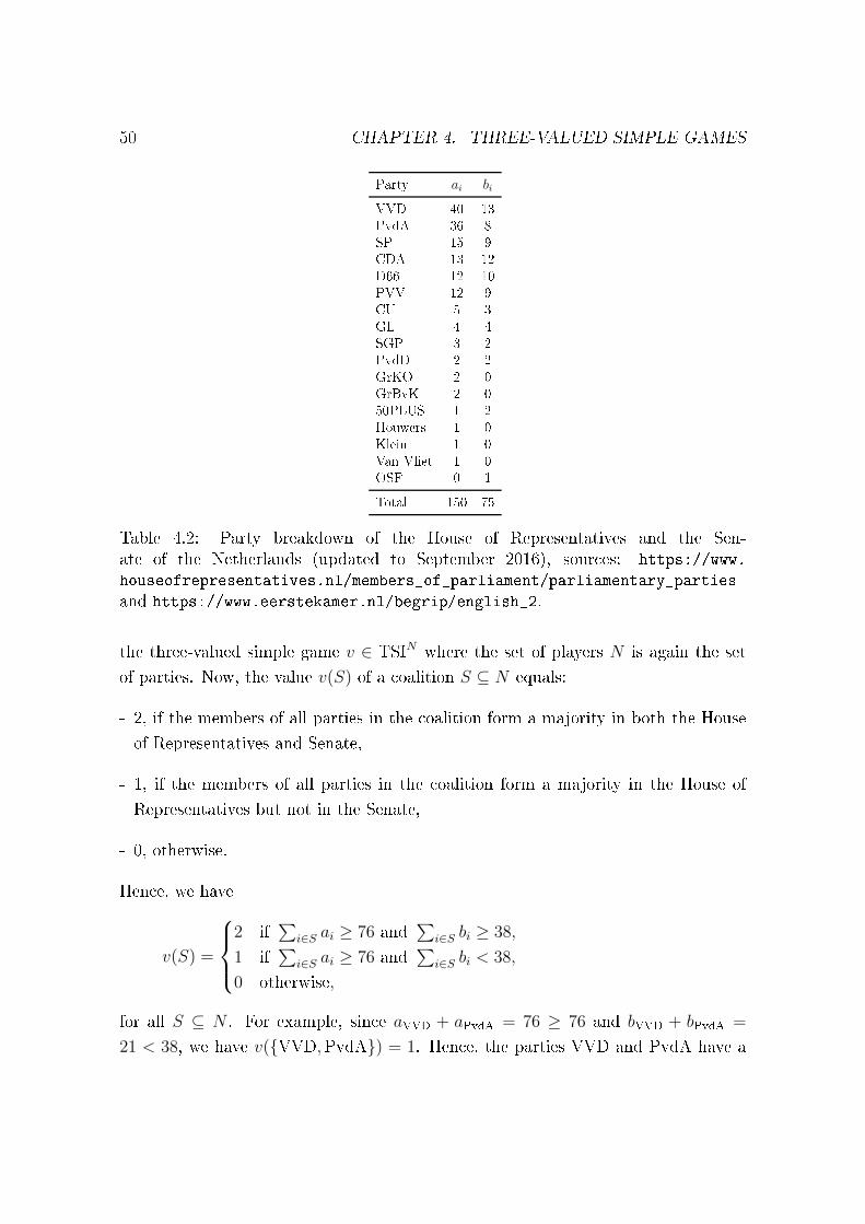
50 CHAPTER 4. THREE-VALUED SIMPLE GAMES
Party ai bi
VVD 40 13PvdA 36 8SP 15 9CDA 13 12D66 12 10PVV 12 9CU 5 3GL 4 4SGP 3 2PvdD 2 2GrKO 2 0GrBvK 2 050PLUS 1 2Houwers 1 0Klein 1 0Van Vliet 1 0OSF 0 1
Total 150 75
Table 4.2: Party breakdown of the House of Representatives and the Sen-ate of the Netherlands (updated to September 2016), sources: https://www.
houseofrepresentatives.nl/members_of_parliament/parliamentary_parties
and https://www.eerstekamer.nl/begrip/english_2.
the three-valued simple game v ∈ TSIN where the set of players N is again the set
of parties. Now, the value v(S) of a coalition S ⊆ N equals:
- 2, if the members of all parties in the coalition form a majority in both the House
of Representatives and Senate,
- 1, if the members of all parties in the coalition form a majority in the House of
Representatives but not in the Senate,
- 0, otherwise.
Hence, we have
v(S) =
2 if
∑i∈S ai ≥ 76 and
∑i∈S bi ≥ 38,
1 if∑
i∈S ai ≥ 76 and∑
i∈S bi < 38,
0 otherwise,
for all S ⊆ N . For example, since aVVD + aPvdA = 76 ≥ 76 and bVVD + bPvdA =
21 < 38, we have v(VVD,PvdA) = 1. Hence, the parties VVD and PvdA have a
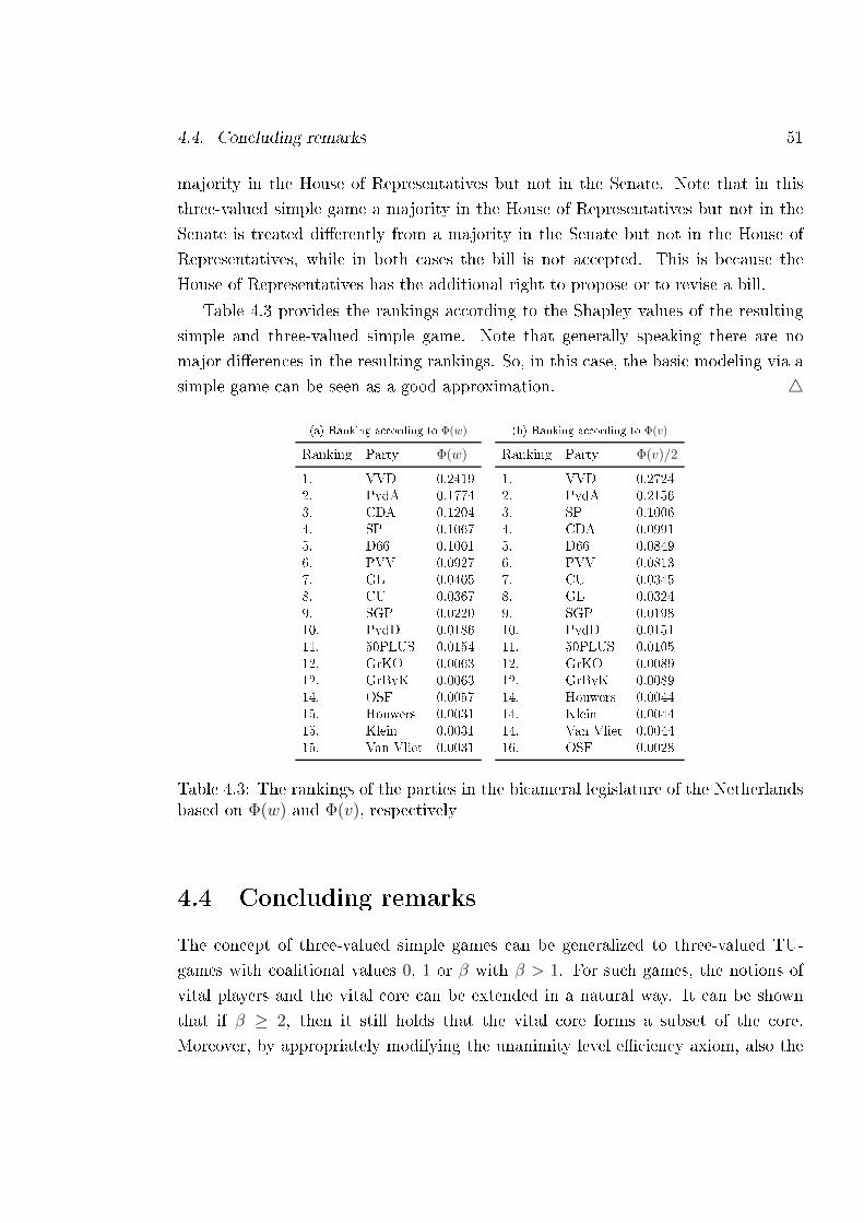
4.4. Concluding remarks 51
majority in the House of Representatives but not in the Senate. Note that in this
three-valued simple game a majority in the House of Representatives but not in the
Senate is treated dierently from a majority in the Senate but not in the House of
Representatives, while in both cases the bill is not accepted. This is because the
House of Representatives has the additional right to propose or to revise a bill.
Table 4.3 provides the rankings according to the Shapley values of the resulting
simple and three-valued simple game. Note that generally speaking there are no
major dierences in the resulting rankings. So, in this case, the basic modeling via a
simple game can be seen as a good approximation. 4
(a) Ranking according to Φ(w)
Ranking Party Φ(w)
1. VVD 0.24192. PvdA 0.17743. CDA 0.12044. SP 0.10675. D66 0.10016. PVV 0.09277. GL 0.04058. CU 0.03679. SGP 0.022010. PvdD 0.018611. 50PLUS 0.015412. GrKO 0.006312. GrBvK 0.006314. OSF 0.005715. Houwers 0.003115. Klein 0.003115. Van Vliet 0.0031
(b) Ranking according to Φ(v)
Ranking Party Φ(v)/2
1. VVD 0.27242. PvdA 0.21563. SP 0.10064. CDA 0.09915. D66 0.08496. PVV 0.08137. CU 0.03458. GL 0.03249. SGP 0.019810. PvdD 0.015111. 50PLUS 0.010512. GrKO 0.008912. GrBvK 0.008914. Houwers 0.004414. Klein 0.004414. Van Vliet 0.004416. OSF 0.0028
Table 4.3: The rankings of the parties in the bicameral legislature of the Netherlandsbased on Φ(w) and Φ(v), respectively
4.4 Concluding remarks
The concept of three-valued simple games can be generalized to three-valued TU-
games with coalitional values 0, 1 or β with β > 1. For such games, the notions of
vital players and the vital core can be extended in a natural way. It can be shown
that if β ≥ 2, then it still holds that the vital core forms a subset of the core.
Moreover, by appropriately modifying the unanimity level eciency axiom, also the
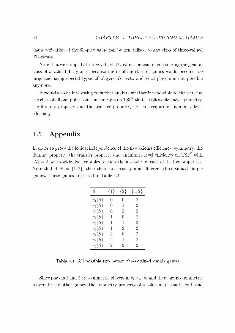
52 CHAPTER 4. THREE-VALUED SIMPLE GAMES
characterization of the Shapley value can be generalized to any class of three-valued
TU-games.
Note that we stopped at three-valued TU-games instead of considering the general
class of k-valued TU-games because the resulting class of games would become too
large and using special types of players like veto and vital players is not possible
anymore.
It would also be interesting to further analyze whether it is possible to characterize
the class of all one-point solution concepts on TSIN that satises eciency, symmetry,
the dummy property and the transfer property, i.e., not requiring unanimity level
eciency.
4.5 Appendix
In order to prove the logical independence of the ve axioms eciency, symmetry, the
dummy property, the transfer property and unanimity level eciency on TSIN with
|N | = 2, we provide ve examples to show the necessity of each of the ve properties.
Note that if N = 1, 2, then there are exactly nine dierent three-valued simple
games. These games are listed in Table 4.4.
S 1 2 1, 2
v1(S) 0 0 2v2(S) 0 1 2v3(S) 0 2 2v4(S) 1 0 2v5(S) 1 1 2v6(S) 1 2 2v7(S) 2 0 2v8(S) 2 1 2v9(S) 2 2 2
Table 4.4: All possible two person three-valued simple games
Since players 1 and 2 are symmetric players in v1, v5, v9 and there are no symmetric
players in the other games, the symmetry property of a solution f is satised if and
4.5. Appendix 53
only if
f1(v1) = f2(v1),
f1(v5) = f2(v5),
f1(v9) = f2(v9).
Likewise, since player 1 is a dummy player in v3 and player 2 is a dummy player in
v7 and there are no dummy players in the other games, the dummy property of a
solution f is satised if and only if
f1(v3) = 0,
f2(v7) = 0.
Moreover, the transfer property boils down to the following nine equalities
f(v2) + f(v4) = f(v1) + f(v5),
f(v2) + f(v7) = f(v1) + f(v8),
f(v3) + f(v4) = f(v1) + f(v6),
f(v3) + f(v5) = f(v2) + f(v6),
f(v3) + f(v7) = f(v1) + f(v9),
f(v3) + f(v8) = f(v2) + f(v9),
f(v5) + f(v7) = f(v4) + f(v8),
f(v6) + f(v7) = f(v4) + f(v9),
f(v6) + f(v8) = f(v5) + f(v9).
Finally, the unanimity level eciency property boils down to the following two equal-
ities
f2(v2) = 1 + 12f2(v1),
f1(v4) = 1 + 12f1(v1).
Example 4.5.1 (Necessity of unanimity level eciency). Consider the one-point
solution concept f , where
f(v1) = f(v2) = f(v4) = f(v5) = f(v9) = (1, 1),
f(v3) = f(v6) = (0, 2),
f(v7) = f(v8) = (2, 0).
Clearly f(v6) 6= Φ(v6) while f satises eciency, symmetry, the dummy property and
the transfer property, but does not satisfy unanimity level eciency. 4
54 CHAPTER 4. THREE-VALUED SIMPLE GAMES
Example 4.5.2 (Necessity of the transfer property). Consider the one-point solution
concept f , where
f(v1) = f(v5) = f(v9) = (1, 1),
f(v2) =(
12, 11
2
),
f(v3) = f(v6) = (0, 2),
f(v4) =(11
2, 1
2
),
f(v7) = f(v8) = (2, 0).
Clearly f(v6) 6= Φ(v6) while f satises eciency, symmetry, the dummy property and
unanimity level eciency, but does not satisfy the transfer property. 4
Example 4.5.3 (Necessity of the dummy property). Consider the one-point solution
concept f , where
f(v1) = f(v5) = f(v6) = f(v8) = f(v9) = (1, 1),
f(v2) = f(v3) =(
12, 11
2
),
f(v4) = f(v7) =(11
2, 1
2
).
Clearly f(v6) 6= Φ(v6) while f satises eciency, symmetry, the transfer property
and unanimity level eciency, but does not satisfy the dummy property. 4
Example 4.5.4 (Necessity of symmetry). Consider the one-point solution concept
f , where
f(v1) = f(v4) = f(v7) = (2, 0),
f(v2) = f(v5) = f(v8) = (1, 1),
f(v3) = f(v6) = f(v9) = (0, 2),
Clearly f(v6) 6= Φ(v6) while f satises eciency, the dummy property, the transfer
property and unanimity level eciency, but does not satisfy symmetry. 4
Example 4.5.5 (Necessity of eciency). Consider the one-point solution concept f ,
where
f(v1) = f(v2) = f(v4) = f(v5) = f(v9) = (2, 2),
f(v3) = f(v6) = (0, 4),
f(v7) = f(v8) = (4, 0),
Clearly f(v6) 6= Φ(v6) while f satises symmetry, the dummy property, the transfer
property and unanimity level eciency, but does not satisfy eciency. 4
Chapter 5
Minimum coloring games
5.1 Introduction
Consider a set of agents who all need access to some type of facility, but some agents
might be in conict. All facilities are similar, but if two agents are in conict, they
cannot have access to the same facility. The total costs are linearly increasing with the
number of facilities used, so the aim is to nd the minimum number of facilities that
can serve all agents. This problem can be modelled by an undirected graph, called the
conict graph, in which the vertices represent the agents. Two vertices are adjacent
if and only if the corresponding agents are in conict. Next, we color all vertices in
such a way that any two adjacent nodes receive dierent colors. Finding the minimum
number of facilities such that every agent has non-conicting access to some facility,
is equivalent to nding a coloring of the vertices of this conict graph that uses the
smallest number of colors. This combinatorial optimization problem is known as
the minimum coloring problem. A survey on minimum coloring problems can, for
example, be found in Randerath and Schiermeyer (2004) and Pardalos, Mavridou,
and Xue (1999). An application of the minimum coloring problem is, for example,
scheduling courses at secondary schools, where some courses are compulsory and other
courses are electives. Courses can be scheduled in any order, but pairs of courses are
in conict in the sense that they can not be assigned to the same time slot if there is
a student who has chosen both courses.
To analyze how to divide the minimal joint costs among the agents, Deng, Ibaraki,
and Nagamochi (1999) introduced minimum coloring games. A minimum coloring
cost game can be seen as an example of a combinatorial optimization or operations
research game. In a combinatorial optimization game, the value of each coalition
55
56 CHAPTER 5. MINIMUM COLORING GAMES
is obtained by solving a combinatorial optimization problem on the corresponding
substructure. A survey on operations research games can be found in Borm, Hamers,
and Hendrickx (2001).
In Deng et al. (1999) the existence of core elements is investigated for the more
general class of combinatorial optimization cost games where the value of a coalition
is dened by an integer program. They showed that such games have a non-empty
core if and only if the associated linear program has an integer optimal solution.
Moreover, in case of bipartite conict graphs, they characterized the core of the
induced minimum coloring games as the convex hull of the characteristic vectors of
the edges in the conict graph. Deng, Ibaraki, Nagamochi, and Zang (2000) studied
total balancedness of minimum coloring games and other combinatorial optimization
games. They showed that a minimum coloring game is totally balanced if and only
if the underlying conict graph is perfect. In Okamoto (2003) concave minimum
coloring games are characterized in terms of forbidden subgraphs. Moreover, for
this case an explicit formula of the Shapley value is provided. In Bietenhader and
Okamoto (2006) core largeness, extendability, and exactness of minimum coloring
games are considered. Okamoto (2008) characterized the core of minimum coloring
games on perfect conict graphs as the convex hull of the characteristic vectors of
the maximum cliques in the conict graph, which is a generalization of the result
by Deng et al. (1999). Additionally, Okamoto (2008) also investigated the nucleolus,
the compromise value and the Shapley value of a minimum coloring game. The most
recent work on minimum coloring games is by Hamers, Miquel, and Norde (2014).
They provided a necessary and sucient condition for a conict graph such that the
induced minimum coloring game has a population monotonic allocation scheme.
The minimum coloring games studied in the works above are cost games. However,
if we assume that in the initial situation no agents share facilities, i.e., every vertex has
its own color, then cooperation in sharing facilities between non-conicting agents will
lead to cost savings. In this chapter, based on Musegaas, Borm, and Quant (2016b),
we dene minimum coloring games as cost savings games instead of cost games and
we focus on conict graphs inducing coalitional cost savings in 0, 1 or 0, 1, 2, i.e.,we focus on simple and three-valued simple minimum coloring games. We investigate
three features of simple and three-valued simple minimum coloring games. First, we
characterize the class of conict graphs inducing such games. For this characteriza-
tion, a distinction is made between perfect and imperfect conict graphs, and the
concept of maximum clique is used. We show that simple minimum coloring games
5.2. Minimum coloring games 57
are always induced by perfect graphs, while three-valued simple minimum coloring
games can be induced by both perfect and imperfect graphs. In particular, there
is only one class of imperfect conict graphs inducing three-valued simple minimum
coloring games. We also provide an upper bound on the number of maximum cliques
for conict graphs inducing simple or three-valued simple games. Second, we char-
acterize the core in terms of the underlying conict graph for these games. This
characterization is also based on the concept of maximum clique. Since simple min-
imum coloring games are always induced by perfect graphs, the characterization of
the core is readily derived. We show that for three-valued simple minimum coloring
games induced by imperfect conict graphs, the core is empty. On the other hand, for
three-valued simple minimum coloring games induced by perfect conict graphs, we
show that the core equals the vital core (cf. Chapter 4). This strengthens the general
relation between the vital core and the core for three-valued simple minimum coloring
games as provided in Theorem 4.2.5. Third, for simple minimum coloring games we
study the decomposition into unanimity games and derive an elegant expression for
the Shapley value.
The organization of this chapter is as follows. Section 5.2 formally introduces
minimum coloring games. In Section 5.3 simple minimum coloring games are inves-
tigated. Finally, Section 5.4 analyzes three-valued simple minimum coloring games.
5.2 Minimum coloring games
In this section we formally dene minimum coloring games. We also provide a survey
of game-theoretic characteristics of minimum coloring games and in particular recall
the characterization of the core of minimum coloring games associated to perfect
conict graphs.
Let G = (N,E) be an undirected graph, called the conict graph. A coloring of
G is a mapping γ : N → N such that γ(i) 6= γ(j) for every i, j ∈ E. The naturalnumbers assigned to the vertices correspond to the colors assigned to the vertices. A
minimum coloring of G is a coloring γ that uses the smallest number of colors, i.e.,
a coloring for which |γ(i) | i ∈ N| is minimal. The number of colors in a minimum
coloring is called the chromatic number of G and is denoted by χ(G). The chromatic
number of a graph is strongly related to the concept of a clique. Note that all vertices
in a maximum clique are mutually adjacent and therefore each of them has to receive
a dierent color in a minimum coloring, so χ(G) ≥ ω(G), for any graph G.
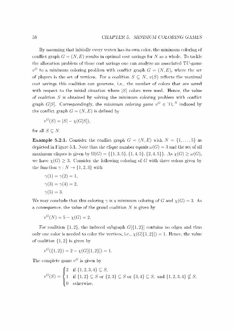
58 CHAPTER 5. MINIMUM COLORING GAMES
By assuming that initially every vertex has its own color, the minimum coloring of
conict graph G = (N,E) results in optimal cost savings for N as a whole. To tackle
the allocation problem of these cost savings one can analyze an associated TU-game
vG to a minimum coloring problem with conict graph G = (N,E), where the set
of players is the set of vertices. For a coalition S ⊆ N , v(S) reects the maximal
cost savings this coalition can generate, i.e., the number of colors that are saved
with respect to the initial situation where |S| colors were used. Hence, the value
of coalition S is obtained by solving the minimum coloring problem with conict
graph G[S]. Correspondingly, the minimum coloring game vG ∈ TUN induced by
the conict graph G = (N,E) is dened by
vG(S) = |S| − χ(G[S]),
for all S ⊆ N .
Example 5.2.1. Consider the conict graph G = (N,E) with N = 1, . . . , 5 as
depicted in Figure 5.1. Note that the clique number equals ω(G) = 3 and the set of all
maximum cliques is given by Ω(G) = 1, 3, 5, 1, 4, 5, 2, 4, 5. As χ(G) ≥ ω(G),
we have χ(G) ≥ 3. Consider the following coloring of G with three colors given by
the function γ : N → 1, 2, 3 with
γ(1) = γ(2) = 1,
γ(3) = γ(4) = 2,
γ(5) = 3.
We may conclude that this coloring γ is a minimum coloring of G and χ(G) = 3. As
a consequence, the value of the grand coalition N is given by
vG(N) = 5− χ(G) = 2.
For coalition 1, 2, the induced subgraph G[1, 2] contains no edges and thus
only one color is needed to color the vertices, i.e., χ(G[1, 2]) = 1. Hence, the value
of coalition 1, 2 is given by
vG(1, 2) = 2− χ(G[1, 2]) = 1.
The complete game vG is given by
vG(S) =
2 if 1, 2, 3, 4 ⊆ S,
1 if 1, 2 ⊆ S or 2, 3 ⊆ S or 3, 4 ⊆ S, and 1, 2, 3, 4 * S,
0 otherwise,
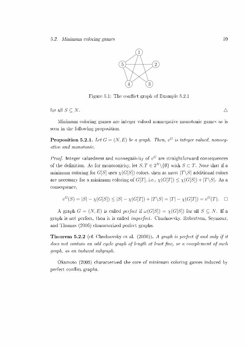
5.2. Minimum coloring games 59
1
2
34
5
Figure 5.1: The conict graph of Example 5.2.1
for all S ⊆ N . 4
Minimum coloring games are integer valued nonnegative monotonic games as is
seen in the following proposition.
Proposition 5.2.1. Let G = (N,E) be a graph. Then, vG is integer valued, nonneg-
ative and monotonic.
Proof. Integer valuedness and nonnegativity of vG are straightforward consequences
of the denition. As for monotonicity, let S, T ∈ 2N\∅ with S ⊂ T . Note that if a
minimum coloring for G[S] uses χ(G[S]) colors, then at most |T\S| additional colorsare necessary for a minimum coloring of G[T ], i.e., χ(G[T ]) ≤ χ(G[S]) + |T\S|. As aconsequence,
vG(S) = |S| − χ(G[S]) ≤ |S| − χ(G[T ]) + |T\S| = |T | − χ(G[T ]) = vG(T ).
A graph G = (N,E) is called perfect if ω(G[S]) = χ(G[S]) for all S ⊆ N . If a
graph is not perfect, then it is called imperfect . Chudnovsky, Robertson, Seymour,
and Thomas (2006) characterized perfect graphs.
Theorem 5.2.2 (cf. Chudnovsky et al. (2006)). A graph is perfect if and only if it
does not contain an odd cycle graph of length at least ve, or a complement of such
graph, as an induced subgraph.
Okamoto (2008) characterized the core of minimum coloring games induced by
perfect conict graphs.
60 CHAPTER 5. MINIMUM COLORING GAMES
Theorem 5.2.3 (cf. Okamoto (2008)). Let G = (N,E) be a perfect graph. Then,
C(vG) = Conv(eN\S | S ∈ Ω(G)
).1
Example 5.2.2. Reconsider the conict graph G = (N,E) in Figure 5.1. Since
G does not contain an odd cycle graph of length at least ve, or a complement
of such graph as an induced subgraph, we know from Theorem 5.2.2 that G is a
perfect conict graph. Since Ω(G) = 1, 3, 5, 1, 4, 5, 2, 4, 5 , it follows from
Theorem 5.2.3 that
C(vG) = Conv((0, 1, 0, 1, 0), (0, 1, 1, 0, 0), (1, 0, 1, 0, 0)). 4
5.3 Simple minimum coloring games
In this section we consider simple minimum coloring games. First, we characterize the
class of conict graphs inducing minimum coloring games that are simple by means
of the chromatic number of the conict graph. We also consider some other features
of this class of conict graphs, for example the number of maximum cliques. After
that, we analyze the core of these induced minimum coloring games and we see that
the veto players are exactly the players who are outside a maximum clique. Finally,
we study the decomposition into unanimity games and derive an elegant expression
for the Shapley value.
The following theorem gives a necessary and sucient condition, in terms of the
chromatic number, for a conict graph to induce a simple minimum coloring game.
Theorem 5.3.1. Let G = (N,E) be a graph. Then, vG ∈ SIN if and only if χ(G) =
n− 1.
Proof. (⇒) Let vG ∈ SIN . Then, vG(N) = 1 and consequently χ(G) = n−vG(N) =
n− 1.
(⇐) Let χ(G) = n−1. Then, vG(N) = n−χ(G) = 1. According to Proposition 5.2.1
vG is integer valued, nonnegative and monotonic, so in particular vG(S) ∈ 0, 1 forall S ⊂ N , which implies vG ∈ SIN .
1Note that the minimum coloring games studied in Okamoto (2008) are cost games, while weconsider minimum coloring games as cost savings games. Hence, the minimum coloring gamesconsidered in this thesis are cost savings games with respect to the standard minimum coloring costgames studied in the literature.
5.3. Simple minimum coloring games 61
Proposition 5.3.3 provides an upper bound on the number of maximum cliques
for conict graphs inducing simple games. This proposition also states that conict
graphs inducing simple games are perfect. In the proof of this proposition we use the
following lemma, which gives the clique number and the chromatic number for odd
cycle graphs of length at least ve and their complements. The proof of this lemma
is straightforward and therefore omitted.
Lemma 5.3.2. Let k ∈ N with k ≥ 2. Then, ω(C2k+1) = 2, χ(C2k+1) = 3,
ω(C2k+1) = k and χ(C2k+1) = k + 1.
Proposition 5.3.3. Let G = (N,E) be a graph. If vG ∈ SIN , then
(i) G is perfect,
(ii) |Ω(G)| ≤ 2.
Proof. Let vG ∈ SIN . Then, according to Theorem 5.3.1, χ(G) = n− 1.
Part (i): Suppose that G is not perfect. Then, according to Theorem 5.2.2, there
exists an S ⊆ N such that G[S] = C2k+1 or G[S] = C2k+1 with k ≥ 2. Then, using
Lemma 5.3.2, we have
vG(S) = |S| − χ(G[S]) = 2k + 1− 3 = 2k − 2 ≥ 2 > vG(N),
in case G[S] = C2k+1, or
vG(S) = |S| − χ(G[S]) = 2k + 1− (k + 1) = k ≥ 2 > vG(N),
in case G[S] = C2k+1, which both contradict monotonicity of vG. Hence, G is perfect.
Part (ii): Since G is perfect (see part (i)) and vG is simple, we have ω(G) = χ(G) =
n − 1. Suppose |Ω(G)| > 2 and let k, l and m be three distinct vertices such that
N\k, N\l and N\m are maximum cliques of G. Since G[N\k] = KN\k
and G[N\l] = KN\l, we have
i, j | i, j ∈ N, i 6= j\k, l ⊆ E.
Moreover, since G[N\m] = KN\m and k, l ⊆ N\m we have k, l ∈ E. Thisimplies G = KN which contradicts χ(G) = n− 1. Hence, |Ω(G)| ≤ 2.
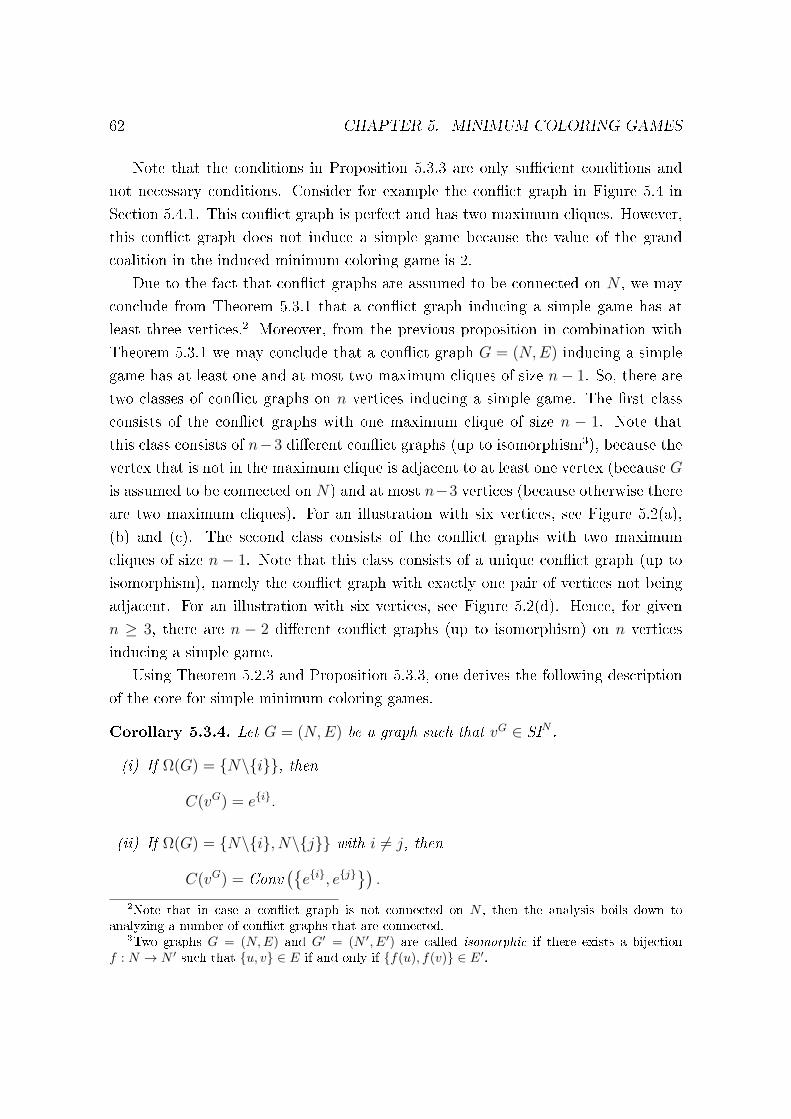
62 CHAPTER 5. MINIMUM COLORING GAMES
Note that the conditions in Proposition 5.3.3 are only sucient conditions and
not necessary conditions. Consider for example the conict graph in Figure 5.4 in
Section 5.4.1. This conict graph is perfect and has two maximum cliques. However,
this conict graph does not induce a simple game because the value of the grand
coalition in the induced minimum coloring game is 2.
Due to the fact that conict graphs are assumed to be connected on N , we may
conclude from Theorem 5.3.1 that a conict graph inducing a simple game has at
least three vertices.2 Moreover, from the previous proposition in combination with
Theorem 5.3.1 we may conclude that a conict graph G = (N,E) inducing a simple
game has at least one and at most two maximum cliques of size n− 1. So, there are
two classes of conict graphs on n vertices inducing a simple game. The rst class
consists of the conict graphs with one maximum clique of size n − 1. Note that
this class consists of n−3 dierent conict graphs (up to isomorphism3), because the
vertex that is not in the maximum clique is adjacent to at least one vertex (because G
is assumed to be connected on N) and at most n−3 vertices (because otherwise there
are two maximum cliques). For an illustration with six vertices, see Figure 5.2(a),
(b) and (c). The second class consists of the conict graphs with two maximum
cliques of size n − 1. Note that this class consists of a unique conict graph (up to
isomorphism), namely the conict graph with exactly one pair of vertices not being
adjacent. For an illustration with six vertices, see Figure 5.2(d). Hence, for given
n ≥ 3, there are n − 2 dierent conict graphs (up to isomorphism) on n vertices
inducing a simple game.
Using Theorem 5.2.3 and Proposition 5.3.3, one derives the following description
of the core for simple minimum coloring games.
Corollary 5.3.4. Let G = (N,E) be a graph such that vG ∈ SIN .
(i) If Ω(G) = N\i, then
C(vG) = ei.
(ii) If Ω(G) = N\i, N\j with i 6= j, then
C(vG) = Conv(ei, ej
).
2Note that in case a conict graph is not connected on N , then the analysis boils down toanalyzing a number of conict graphs that are connected.
3Two graphs G = (N,E) and G′ = (N ′, E′) are called isomorphic if there exists a bijectionf : N → N ′ such that u, v ∈ E if and only if f(u), f(v) ∈ E′.
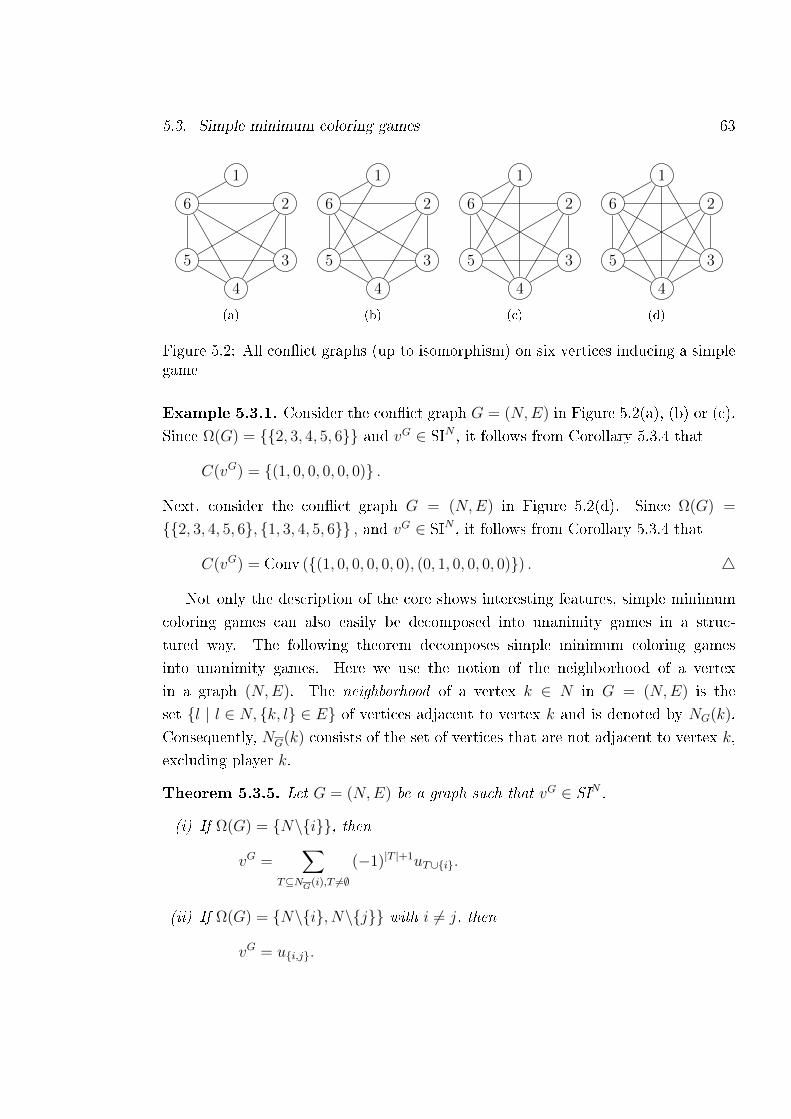
5.3. Simple minimum coloring games 63
1
2
3
4
5
6
(a)
1
2
3
4
5
6
(b)
1
2
3
4
5
6
(c)
1
2
3
4
5
6
(d)
Figure 5.2: All conict graphs (up to isomorphism) on six vertices inducing a simplegame
Example 5.3.1. Consider the conict graph G = (N,E) in Figure 5.2(a), (b) or (c).
Since Ω(G) = 2, 3, 4, 5, 6 and vG ∈ SIN , it follows from Corollary 5.3.4 that
C(vG) = (1, 0, 0, 0, 0, 0) .
Next, consider the conict graph G = (N,E) in Figure 5.2(d). Since Ω(G) =
2, 3, 4, 5, 6, 1, 3, 4, 5, 6 , and vG ∈ SIN , it follows from Corollary 5.3.4 that
C(vG) = Conv ((1, 0, 0, 0, 0, 0), (0, 1, 0, 0, 0, 0)) . 4
Not only the description of the core shows interesting features, simple minimum
coloring games can also easily be decomposed into unanimity games in a struc-
tured way. The following theorem decomposes simple minimum coloring games
into unanimity games. Here we use the notion of the neighborhood of a vertex
in a graph (N,E). The neighborhood of a vertex k ∈ N in G = (N,E) is the
set l | l ∈ N, k, l ∈ E of vertices adjacent to vertex k and is denoted by NG(k).
Consequently, NG(k) consists of the set of vertices that are not adjacent to vertex k,
excluding player k.
Theorem 5.3.5. Let G = (N,E) be a graph such that vG ∈ SIN .
(i) If Ω(G) = N\i, then
vG =∑
T⊆NG(i),T 6=∅
(−1)|T |+1uT∪i.
(ii) If Ω(G) = N\i, N\j with i 6= j, then
vG = ui,j.
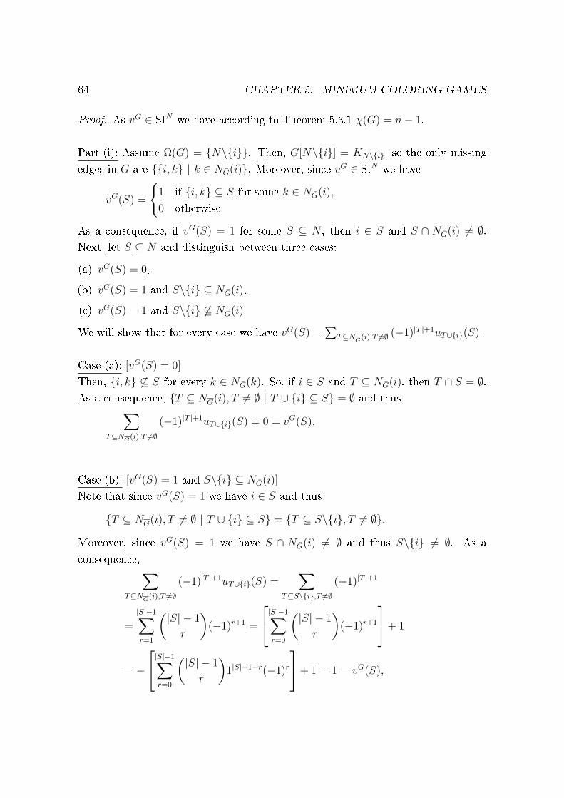
64 CHAPTER 5. MINIMUM COLORING GAMES
Proof. As vG ∈ SIN we have according to Theorem 5.3.1 χ(G) = n− 1.
Part (i): Assume Ω(G) = N\i. Then, G[N\i] = KN\i, so the only missing
edges in G are i, k | k ∈ NG(i). Moreover, since vG ∈ SIN we have
vG(S) =
1 if i, k ⊆ S for some k ∈ NG(i),
0 otherwise.
As a consequence, if vG(S) = 1 for some S ⊆ N , then i ∈ S and S ∩ NG(i) 6= ∅.Next, let S ⊆ N and distinguish between three cases:
(a) vG(S) = 0,
(b) vG(S) = 1 and S\i ⊆ NG(i),
(c) vG(S) = 1 and S\i 6⊆ NG(i).
We will show that for every case we have vG(S) =∑
T⊆NG(i),T 6=∅ (−1)|T |+1uT∪i(S).
Case (a): [vG(S) = 0]
Then, i, k 6⊆ S for every k ∈ NG(k). So, if i ∈ S and T ⊆ NG(i), then T ∩ S = ∅.As a consequence, T ⊆ NG(i), T 6= ∅ | T ∪ i ⊆ S = ∅ and thus∑
T⊆NG(i),T 6=∅
(−1)|T |+1uT∪i(S) = 0 = vG(S).
Case (b): [vG(S) = 1 and S\i ⊆ NG(i)]
Note that since vG(S) = 1 we have i ∈ S and thus
T ⊆ NG(i), T 6= ∅ | T ∪ i ⊆ S = T ⊆ S\i, T 6= ∅.
Moreover, since vG(S) = 1 we have S ∩ NG(i) 6= ∅ and thus S\i 6= ∅. As a
consequence,∑T⊆NG(i),T 6=∅
(−1)|T |+1uT∪i(S) =∑
T⊆S\i,T 6=∅
(−1)|T |+1
=
|S|−1∑r=1
(|S| − 1
r
)(−1)r+1 =
|S|−1∑r=0
(|S| − 1
r
)(−1)r+1
+ 1
= −
|S|−1∑r=0
(|S| − 1
r
)1|S|−1−r(−1)r
+ 1 = 1 = vG(S),
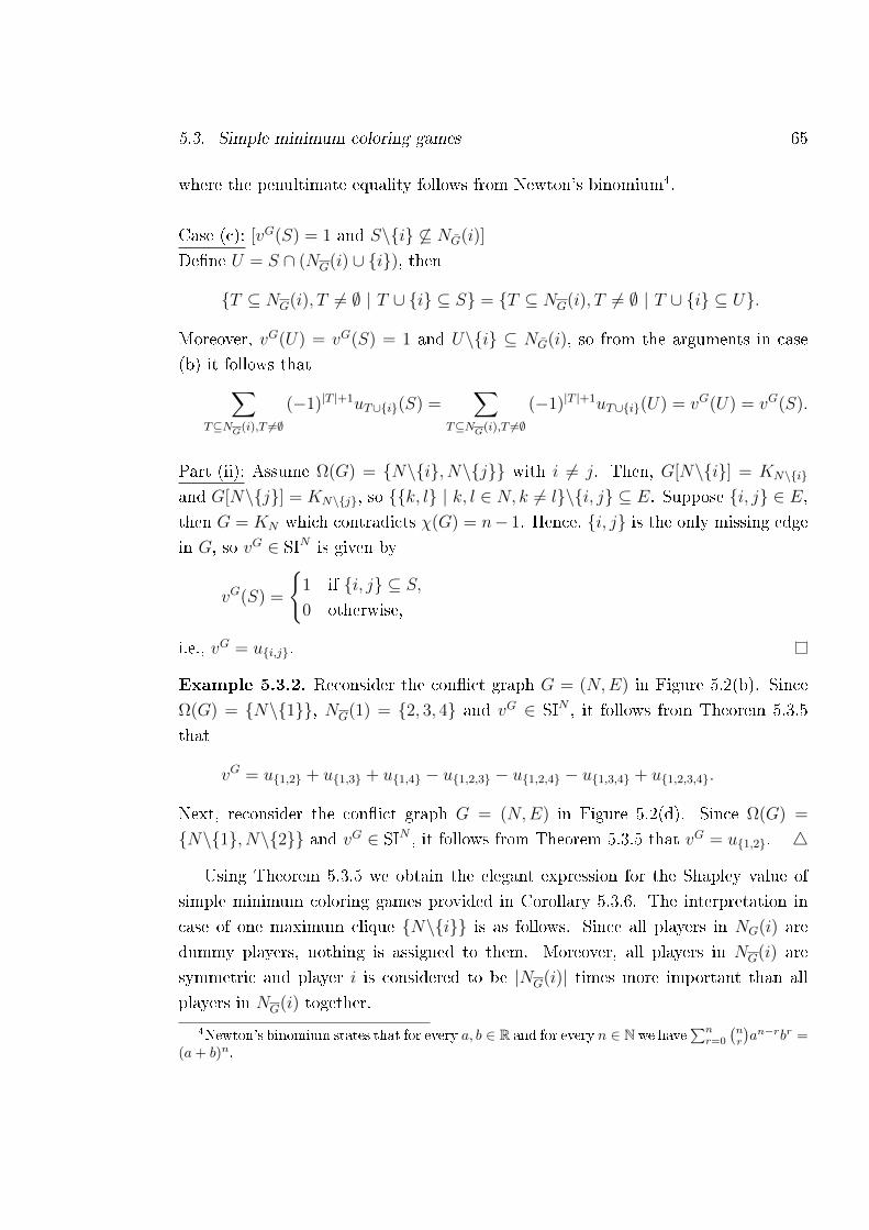
5.3. Simple minimum coloring games 65
where the penultimate equality follows from Newton's binomium4.
Case (c): [vG(S) = 1 and S\i 6⊆ NG(i)]
Dene U = S ∩ (NG(i) ∪ i), then
T ⊆ NG(i), T 6= ∅ | T ∪ i ⊆ S = T ⊆ NG(i), T 6= ∅ | T ∪ i ⊆ U.
Moreover, vG(U) = vG(S) = 1 and U\i ⊆ NG(i), so from the arguments in case
(b) it follows that∑T⊆NG(i),T 6=∅
(−1)|T |+1uT∪i(S) =∑
T⊆NG(i),T 6=∅
(−1)|T |+1uT∪i(U) = vG(U) = vG(S).
Part (ii): Assume Ω(G) = N\i, N\j with i 6= j. Then, G[N\i] = KN\i
and G[N\j] = KN\j, so k, l | k, l ∈ N, k 6= l\i, j ⊆ E. Suppose i, j ∈ E,then G = KN which contradicts χ(G) = n− 1. Hence, i, j is the only missing edge
in G, so vG ∈ SIN is given by
vG(S) =
1 if i, j ⊆ S,
0 otherwise,
i.e., vG = ui,j.
Example 5.3.2. Reconsider the conict graph G = (N,E) in Figure 5.2(b). Since
Ω(G) = N\1, NG(1) = 2, 3, 4 and vG ∈ SIN , it follows from Theorem 5.3.5
that
vG = u1,2 + u1,3 + u1,4 − u1,2,3 − u1,2,4 − u1,3,4 + u1,2,3,4.
Next, reconsider the conict graph G = (N,E) in Figure 5.2(d). Since Ω(G) =
N\1, N\2 and vG ∈ SIN , it follows from Theorem 5.3.5 that vG = u1,2. 4
Using Theorem 5.3.5 we obtain the elegant expression for the Shapley value of
simple minimum coloring games provided in Corollary 5.3.6. The interpretation in
case of one maximum clique N\i is as follows. Since all players in NG(i) are
dummy players, nothing is assigned to them. Moreover, all players in NG(i) are
symmetric and player i is considered to be |NG(i)| times more important than all
players in NG(i) together.
4Newton's binomium states that for every a, b ∈ R and for every n ∈ N we have∑nr=0
(nr
)an−rbr =
(a+ b)n.
66 CHAPTER 5. MINIMUM COLORING GAMES
Corollary 5.3.6. Let G = (N,E) be a graph such that vG ∈ SIN .
(i) If Ω(G) = N\i, then for k ∈ N we have
Φk(vG) =
|NG(i)||NG(i)|+1
if k = i,1
|NG(i)|(|NG(i)|+1)if k ∈ NG(i),
0 if k ∈ NG(i).
(ii) If Ω(G) = N\i, N\j with i 6= j, then for k ∈ N we have
Φk(vG) =
12
if k ∈ i, j,0 otherwise.
Proof. Part (i): Assume Ω(G) = N\i and let k ∈ N . Then, from Theorem 5.3.5
it follows that vG =∑
T⊆NG(i),T 6=∅ (−1)|T |+1uT∪i. By (2.5) we have
Φi(vG) =
∑T⊆NG(i),T 6=∅
(−1)|T |+1
|T |+ 1=
NG(i)∑r=1
(−1)r+1
r + 1
(|NG(i)|
r
)
=
|NG(i)|∑r=1
(−1)r+1
|NG(i)|+ 1
(|NG(i)|+ 1
r + 1
)
=1
|NG(i)|+ 1
|NG(i)|+1∑r=2
(−1)r(|NG(i)|+ 1
r
)=
1
|NG(i)|+ 1
|NG(i)|+1∑r=0
(−1)r(|NG(i)|+ 1
r
)− 1 + (|NG(i)|+ 1)
=
1
|NG(i)|+ 1(0− 1 + (|NG(i)|+ 1)) =
|NG(i)||NG(i)|+ 1
,
where the second to last equality follows from Newton's binomium.
For k ∈ NG(i) we have k 6∈ S for every S ∈ T ∪ i | T ⊆ NG(i), T 6= ∅.Therefore, using (2.5), we have Φk(v
G) = 0 for every k ∈ NG(i).
Because of eciency we know∑
k∈NG(i) Φk(vG) = 1 − |NG(i)|
|NG(i)|+1= 1|NG(i)|+1
. Note
that all players in NG(i) are symmetric. Therefore, due to symmetry we have
Φk(vG) =
1|NG(i)|+1
|NG(i)|=
1
|NG(i)|(|NG(i)|+ 1).
5.4. Three-valued simple minimum coloring games 67
Part (ii): Assume Ω(G) = N\i, N\j with i 6= j. Then, from Theorem 5.3.5 it
follows that vG = ui,j. Therefore, from the denition of the Shapley value in (2.5)
Φ(vG) follows directly.
Note that for a conict graph G = (N,E) that induces a simple game and has one
maximum clique N\i we have NG(i) 6= ∅ and thus, using the previous corollary,
Φi(vG) < 1. By Corollary 5.3.4 this implies Φ(vG) 6∈ C(vG).
5.4 Three-valued simple minimum coloring games
In this section we characterize the class of conict graphs inducing three-valued simple
minimum coloring games by means of the chromatic number of the conict graph.
For this, a distinction is made between perfect and imperfect conict graphs. After
that, we characterize the core in terms of the underlying conict graph for these
games.
The following theorem gives a necessary and sucient condition, in terms of the
chromatic number, for a conict graph to induce a three-valued simple game.
Theorem 5.4.1. Let G = (N,E) be a graph. Then, vG ∈ TSIN if and only if
χ(G) = n− 2.5
Proof. (⇒) Let vG ∈ TSIN . Then, vG(N) = 2 and consequently χ(G) = n −vG(N) = n− 2.
(⇐) Let χ(G) = n−2. Then, vG(N) = n−χ(G) = 2. According to Proposition 5.2.1
vG is integer valued, nonnegative and monotonic, so in particular vG(S) ∈ 0, 1, 2for all S ⊂ N , which implies vG ∈ TSIN .
From now on, we distinguish between two classes of conict graphs inducing three-
valued simple minimum coloring games: perfect conict graphs (Section 5.4.1) and
imperfect conict graphs (Section 5.4.2). For both classes, we consider in more detail
the structure of these conict graphs and the cores of the induced minimum coloring
games.
5Note that Theorem 5.3.1 and Theorem 5.4.1 can be generalized for a more general class ofinteger valued, nonnegative and monotonic games.
68 CHAPTER 5. MINIMUM COLORING GAMES
5.4.1 Three-valued simple minimum coloring games induced
by perfect conict graphs
In this section we consider three-valued simple minimum coloring games induced by
perfect conict graphs. We consider a specic feature of this class of conict graphs,
namely the number of maximum cliques. After that we analyze the core and the vital
core and we see that the core and the vital core coincide.
We start with providing an upper bound on the number of maximum cliques for
perfect conict graphs inducing three-valued simple games.
Proposition 5.4.2. Let G = (N,E) be a perfect graph. If vG ∈ TSIN , then |Ω(G)| ≤4.
Proof. Let vG ∈ TSIN . Then, using Theorem 5.4.1, χ(G) = n − 2. Hence, due to
the fact that G is assumed to be connected on N , we have n ≥ 4. Moreover, since
G is perfect, we have ω(G) = χ(G) = n− 2, so at least two pairs of vertices are not
adjacent in G. Without loss of generality we can assume that either 1, 2 6∈ E and
3, 4 6∈ E, or 1, 2 6∈ E and 2, 3 6∈ E. Therefore, we distinguish between these
two cases and we show that for both cases we have |Ω(G)| ≤ 4.
Case (a): [1, 2 6∈ E and 3, 4 6∈ E]Then the sets of vertices that can possibly form a maximum clique are
T ⊆ N | |T | = n− 2, 1, 2 * T, 3, 4 * T.
Therefore, a maximum clique is of the form N\i, j with i ∈ 1, 2 and j ∈ 3, 4.Hence, there are only four sets of vertices that can possibly form a maximum clique,
i.e., |Ω(G)| ≤ 4.
Case (b): [1, 2 6∈ E and 2, 3 6∈ E]Since N\2 cannot form a clique, we know that there exists a pair of vertices i, j ⊆N\2 with i 6= j and i, j 6∈ E. Hence, without loss of generality we can assume
that 1, 3 6∈ E, 3, 4 6∈ E or 4, 5 6∈ E (the last case is only possible if n ≥ 5). Note
that if 3, 4 6∈ E or 4, 5 6∈ E, then we are back to case (a) and thus |Ω(G)| ≤ 4.
If 1, 3 6∈ E, then the sets of vertices that can possibly form a maximum clique are
T ⊆ N | |T | = n− 2, 1, 2 * T, 1, 3 * T, 2, 3 * T.
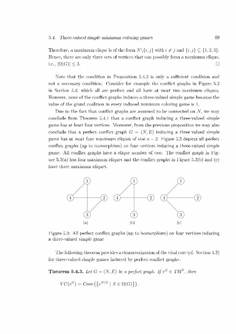
5.4. Three-valued simple minimum coloring games 69
Therefore, a maximum clique is of the form N\i, j with i 6= j and i, j ⊆ 1, 2, 3.Hence, there are only three sets of vertices that can possibly form a maximum clique,
i.e., |Ω(G)| ≤ 3.
Note that the condition in Proposition 5.4.2 is only a sucient condition and
not a necessary condition. Consider for example the conict graphs in Figure 5.2
in Section 5.3, which all are perfect and all have at most two maximum cliques.
However, none of the conict graphs induces a three-valued simple game because the
value of the grand coalition in every induced minimum coloring game is 1.
Due to the fact that conict graphs are assumed to be connected on N , we may
conclude from Theorem 5.4.1 that a conict graph inducing a three-valued simple
game has at least four vertices. Moreover, from the previous proposition we may also
conclude that a perfect conict graph G = (N,E) inducing a three-valued simple
game has at most four maximum cliques of size n− 2. Figure 5.3 depicts all perfect
conict graphs (up to isomorphism) on four vertices inducing a three-valued simple
game. All conict graphs have a clique number of two. The conict graph in Fig-
ure 5.3(a) has four maximum cliques and the conict graphs in Figure 5.3(b) and (c)
have three maximum cliques.
1
2
3
4
(a)
1
2
3
4
(b)
1
2
3
4
(c)
Figure 5.3: All perfect conict graphs (up to isomorphism) on four vertices inducinga three-valued simple game
The following theorem provides a characterization of the vital core (cf. Section 4.2)
for three-valued simple games induced by perfect conict graphs.
Theorem 5.4.3. Let G = (N,E) be a perfect graph. If vG ∈ TSIN , then
V C(vG) = Conv(eN\S | S ∈ Ω(G)
).
70 CHAPTER 5. MINIMUM COLORING GAMES
Proof. Let vG ∈ TSIN . Then, using Theorem 5.4.1 and the fact that G is perfect, we
have ω(G) = χ(G) = n− 2. In this proof we denote the intersection of all maximum
cliques in G by ΩG, i.e.,
ΩG =⋂S | S ∈ Ω(G).
We divide the proof into proving the following four statements:
(i) Vit(vG) = N\ΩG,
(ii) vG is permissible,
(iii) PVit(vG) = ∅,
(iv) SVit(vG) = N\S | S ∈ Ω(G).
Note that if the statements (i) - (iv) all hold, then it immediately follows from the
denition of the vital core that V C(vG) = Conv(eN\S | S ∈ Ω(G)
).
Part (i): [Vit(vG) = N\ΩG]
(⊂) Let i ∈ ΩG, i.e., i belongs to every maximum clique of G. This implies that if
vertex i is removed, then the clique number decreases with one. Therefore,
vG(N\i) = n− 1− χ(G[N\i]) = n− 1− ω(G[N\i])= n− 1− (ω(G)− 1) = n− 1− (χ(G)− 1) = n− 1− (n− 3) = 2,
where the second and the fourth equalities follow from the fact that G is perfect.
Hence, there exists an S ⊆ N\i such that vG(S) = 2, so i 6∈ Vit(vG).
(⊃) Let i ∈ N\ΩG, i.e., there exists a maximum clique of G to which i does not
belong. This implies that if vertex i is removed, then the clique number does not
change. Therefore,
vG(N\i) = n− 1− χ(G[N\i]) = n− 1− ω(G[N\i])= n− 1− ω(G) = n− 1− χ(G) = n− 1− (n− 2) = 1,
where the second and the fourth equalities follow from the fact that G is perfect.
Moreover, from monotonicity of vG it follows that vG(S) ≤ 1 for all S ⊆ N\i, sothere does not exist an S ⊆ N\i with v(S) = 2. As a consequence, for all S ⊆ N
with v(S) = 2 we have i ∈ S and thus i ∈ Vit(vG).
5.4. Three-valued simple minimum coloring games 71
Part (ii): [vG is permissible]
Since ω(G) = n− 2, we know that N cannot be a maxium clique and thus ΩG 6= N .
Hence, Vit(vG) = N\ΩG 6= ∅. Moreover, since ΩG is the intersection of all maximum
cliques in G, we know that ΩG forms a clique as well and thus χ(G[ΩG]) = |ΩG|. Asa consequence, vG(N\Vit(vG)) = vG(ΩG) = 0. This implies that vG is permissible.
Part (iii): [PVit(vG) = ∅]Since Vit(vG) = N\ΩG, we know that for every vital player there exists a maximum
clique of G to which this player does not belong. As a consequence, for i ∈ Vit(vG),
we have
χ(G[N\i]) = ω(G[N\i]) = ω(G) = n− 2,
where the rst equality follows from the fact that G is perfect and the second equality
follows from the fact that there exists a maximum clique of G to which i does not
belong. Therefore,
vGr (Vit(vG)\i) = vG(Vit(vG)\i ∪ (N\Vit(vG))) = vG(N\i)= n− 1− χ(G[N\i]) = n− 1− (n− 2) = 1,
for all i ∈ Vit(vG). As a consequence,
PVit(vG) =⋂
S ⊆ Vit(v) | vGr (S) ∈ 1, 2⊆⋂
Vit(vG)\i | i ∈ Vit(vG)
= ∅.
Part (iv): [SVit(vG) = N\S | S ∈ Ω(G)](⊃) Let S ∈ Ω(G). Since ω(G) = n − 2, we can denote N\S = i, j with i 6= j.
Note i, j ∩ ΩG = ∅ and thus i, j ⊆ Vit(vG). Moreover, since PVit(vG) = ∅, wehave i, j ⊆ Vit(vG)\PVit(vG). Suppose i, j 6∈ SVit(vG), then it follows from
the denition of secondary vital pairs that there exists a T ⊆ Vit(vG)\i, j with
vGr (T ) = 1. Since T ⊆ Vit(vG)\i, j, we have
(T ∪ ΩG) ⊆ ((Vit(vG)\i, j) ∪ ΩG) = N\i, j = S.
Moreover, since S forms a maximum clique in G, we have χ(G[T ∪ ΩG]) = |T ∪ ΩG|and thus
vGr (T ) = vG(T ∪ (N\Vit(vG))) = vG(T ∪ ΩG) = |T ∪ ΩG| − χ(G[T ∪ ΩG])
= |T ∪ ΩG| − |T ∪ ΩG| = 0,
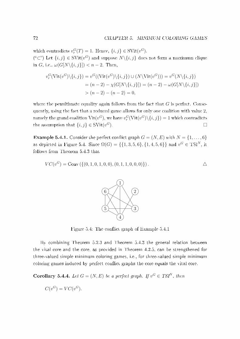
72 CHAPTER 5. MINIMUM COLORING GAMES
which contradicts vGr (T ) = 1. Hence, i, j ∈ SVit(vG).
(⊂) Let i, j ∈ SVit(vG) and suppose N\i, j does not form a maximum clique
in G, i.e., ω(G[N\i, j]) < n− 2. Then,
vGr (Vit(vG)\i, j) = vG((Vit(vG)\i, j) ∪ (N\Vit(vG))) = vG(N\i, j)= (n− 2)− χ(G[N\i, j]) = (n− 2)− ω(G[N\i, j])> (n− 2)− (n− 2) = 0,
where the penultimate equality again follows from the fact that G is perfect. Conse-
quently, using the fact that a reduced game allows for only one coalition with value 2,
namely the grand coalition Vit(vG), we have vGr (Vit(vG)\i, j) = 1 which contradicts
the assumption that i, j ∈ SVit(vG).
Example 5.4.1. Consider the perfect conict graph G = (N,E) with N = 1, . . . , 6as depicted in Figure 5.4. Since Ω(G) = 1, 3, 5, 6, 1, 4, 5, 6 and vG ∈ TSIN , it
follows from Theorem 5.4.3 that
V C(vG) = Conv ((0, 1, 0, 1, 0, 0), (0, 1, 1, 0, 0, 0)) . 4
1
2
3
4
5
6
Figure 5.4: The conict graph of Example 5.4.1
By combining Theorem 5.2.3 and Theorem 5.4.3 the general relation between
the vital core and the core, as provided in Theorem 4.2.5, can be strengthened for
three-valued simple minimum coloring games, i.e., for three-valued simple minimum
coloring games induced by perfect conict graphs the core equals the vital core.
Corollary 5.4.4. Let G = (N,E) be a perfect graph. If vG ∈ TSIN , then
C(vG) = V C(vG).
5.4. Three-valued simple minimum coloring games 73
5.4.2 Three-valued simple minimum coloring games induced
by imperfect conict graphs
In this section we consider three-valued simple minimum coloring games induced
by imperfect conict graphs. First, we characterize this class of conict graphs.
Moreover, we show that for a given number n ≥ 5 of vertices the class of imperfect
conict graphs on n vertices inducing a three-valued simple game consists of a unique
conict graph. Next, we show that the induced minimum coloring games are never
permissible and thus always have an empty core.
Note that all imperfect graphs have at least ve vertices, because it must contain
an odd cycle graph of length at least ve, or a complement of such graph as an
induced subgraph (cf. Theorem 5.2.2). The following theorem provides a necessary
and sucient condition for an imperfect conict graph to induce a three-valued simple
game. For this theorem, we use the notion of a dominating vertex. A vertex i ∈ Nis called dominating in G if j | j ∈ N, i, j ∈ E = N\i, i.e., if i is adjacent toevery other vertex.
Theorem 5.4.5. Let G = (N,E) be an imperfect graph. Then, vG ∈ TSIN if and
only if there exists an S ⊆ N such that G[S] = C5 and all vertices outside S are
dominating.
Proof. (⇐) Let S ⊆ N be such that G[S] = C5 and let all vertices outside S be
dominating. Since all vertices in N\S are dominating, we have G[N\S] = KN\S and
thus χ(G[N\S]) = n− 5. Moreover, since each vertex in S is adjacent to each vertex
in N\S, we have
χ(G) = χ(G[N\S]) + χ(G[S]) = n− 5 + 3 = n− 2,
where the second equality follows from Lemma 5.3.2. Consequently, using Theo-
rem 5.4.1, we have vG ∈ TSIN .
(⇒) Let vG ∈ TSIN . Since G is not perfect, we know from Theorem 5.2.2 that
there exists an S ⊆ N such that G[S] = C2k+1 or G[S] = C2k+1 with k ≥ 2. Suppose
k > 2. Then, using Lemma 5.3.2, we have
vG(S) = |S| − χ(G[S]) = 2k + 1− 3 = 2k − 2 > 2,
in case G[S] = C2k+1, or
vG(S) = |S| − χ(G[S]) = 2k + 1− (k + 1) = k > 2,
74 CHAPTER 5. MINIMUM COLORING GAMES
in case G[S] = C2k+1, which both contradict vG being a three-valued simple game.
Hence, k = 2 and thus G[S] = C5 or G[S] = C5. Since C5 and C5 are isomorphic to
each other6, and thus both graphs have the same clique and chromatic number, we
can conclude that G[S] = C5.
Now, suppose χ(G[N\S]) < |N\S| = n− 5. Then
vG(N) = n− χ(G) ≥ n− (χ(G[S]) + χ(G[N\S])) > n− (3 + n− 5) = 2,
which contradicts vG being a three-valued simple game. Hence, we may assume
χ(G[N\S]) = n− 5 and thus G[N\S] = KN\S. As a consequence, all players in N\Smutually adjacent, i.e.,
j | j ∈ N\S, i, j ∈ E = (N\S)\i,
for all i ∈ N\S.Next, suppose i, j 6∈ E for some i ∈ S and j ∈ N\S. Then, since there exists
a vertex in S that is not adjacent to a vertex in N\S, those two players can receive
the same color in the minimum coloring of G. Hence, χ(G) < χ(G[S]) + χ(G[N\S])
and thus
vG(N) = n− χ(G) > n− (χ(G[S]) + χ(G[N\S])) = n− (3 + n− 5) = 2,
which again contradicts vG being a three-valued simple game. Hence, we may assume
that every player in N\S is adjacent to all players in S, i.e.,
j | j ∈ S, i, j ∈ E = S,
for all i ∈ N\S. Consequently,
j | j ∈ N, i, j ∈ E = N\i,
for all i ∈ N\S, i.e., all vertices outside S are dominating.
6To see that C5 and C5 are isomorphic to each other, consider the graphs G = (N,E) andG′ = (N ′, E′) with N = N ′ = 1, . . . , 5,
E = 1, 2, 1, 5, 2, 3, 3, 4, 4, 5,
and
E′ = 1, 3, 1, 4, 2, 4, 2, 5, 3, 5.
If one takes the bijection f : N → N ′ with f(1) = 1, f(2) = 3, f(3) = 5, f(4) = 2 and f(5) = 4,then u, v ∈ E if and only if f(u), f(v) ∈ E′.
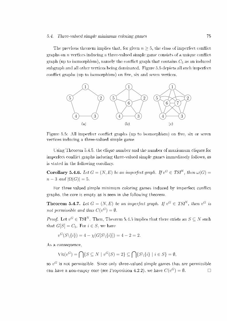
5.4. Three-valued simple minimum coloring games 75
The previous theorem implies that, for given n ≥ 5, the class of imperfect conict
graphs on n vertices inducing a three-valued simple game consists of a unique conict
graph (up to isomorphism), namely the conict graph that contains C5 as an induced
subgraph and all other vertices being dominated. Figure 5.5 depicts all such imperfect
conict graphs (up to isomorphism) on ve, six and seven vertices.
1
2
34
5
(a)
1
2
34
56
(b)
1
2
34
56 7
(c)
Figure 5.5: All imperfect conict graphs (up to isomorphism) on ve, six or sevenvertices inducing a three-valued simple game
Using Theorem 5.4.5, the clique number and the number of maxiumum cliques for
imperfect conict graphs inducing three-valued simple games immediately follows, as
is stated in the following corollary.
Corollary 5.4.6. Let G = (N,E) be an imperfect graph. If vG ∈ TSIN , then ω(G) =
n− 3 and |Ω(G)| = 5.
For three-valued simple minimum coloring games induced by imperfect conict
graphs, the core is empty as is seen in the following theorem.
Theorem 5.4.7. Let G = (N,E) be an imperfect graph. If vG ∈ TSIN , then vG is
not permissible and thus C(vG) = ∅.
Proof. Let vG ∈ TSIN . Then, Theorem 5.4.5 implies that there exists an S ⊆ N such
that G[S] = C5. For i ∈ S, we have
vG(S\i) = 4− χ(G[S\i]) = 4− 2 = 2.
As a consequence,
Vit(vG) =⋂S ⊆ N | vG(S) = 2 ⊆
⋂S\i | i ∈ S = ∅,
so vG is not permissible. Since only three-valued simple games that are permissible
can have a non-empty core (see Proposition 4.2.2), we have C(vG) = ∅.

Chapter 6
Step out - Step in sequencing games
6.1 Introduction
In this chapter one-machine sequencing situations are considered with a queue of
players in front of a single machine, each with one job to be processed. Such a situa-
tion species for each player the processing time, time the machine takes to process
the corresponding job of this player. In addition, it is assumed that each player has
a linear cost function specied by an individual cost parameter. To minimize total
joint costs, Smith (1956) showed that the players must be ordered with respect to
weakly decreasing urgency, dened as the ratio of the individual cost parameter and
the processing time. Assuming the presence of an initial order, this reordering will
lead to cost savings. To analyze how to divide the maximal cost savings among the
players, Curiel et al. (1989) introduced cooperative sequencing games. They show
that sequencing games are convex and therefore have a non-empty core. This means
that it is always possible to nd a coalitionally stable cost savings division.
Several variants of classical classes of sequencing problems and games have been
discussed in the literature. These classes are all based on dierent features of the
underlying sequencing situations, for example by imposing restrictive assumptions
on the jobs, grouping of jobs, stochastic data, dynamic/multistage situations, mul-
tiple jobs and/or machines. Namely, Hamers, Borm, and Tijs (1995) imposed ready
times on the jobs, Borm, Fiestras-Janeiro, Hamers, Sánchez, and Voorneveld (2002)
imposed due dates on the jobs and Hamers, Klijn, and Van Velzen (2005) imposed
precedence constraints on the jobs. Both Gerichhausen and Hamers (2009) and Grun-
del, Çiftçi, Borm, and Hamers (2013) applied grouping of jobs, but in a dier-
ent way. Gerichhausen and Hamers (2009) considered partitioning sequencing games
77
78 CHAPTER 6. STEP OUT - STEP IN SEQUENCING GAMES
where certain batches of jobs have some privilege over other batches of jobs. Grundel
et al. (2013) introduced family sequencing situations and included the concept of set-
up times in their model. Alparslan-Gök, Branzei, Fragnelli, and Tijs (2013) and Klijn
and Sánchez (2006) considered stochastic data in sequencing games. Alparslan-Gök
et al. (2013) considered sequencing games where uncertainty in the parameters (costs
per time unit and/or processing time) is involved by means of interval data. Klijn and
Sánchez (2006) considered uncertainty sequencing situations, i.e., sequencing situa-
tions in which no initial order is specied. In multi-stage sequencing situations, the
order arrived at after each stage becomes the starting order for the next stage. Multi-
stage sequencing situations are for example considered by Curiel (2015). In Lohmann,
Borm, and Slikker (2014) another type of dynamic sequencing situations is consid-
ered, in which a player enters the system at the moment the player starts to prepare
the machine for his job (there is a predecessor dependent set-up time) and leaves
the system as soon as his job is nished. Çiftçi, Borm, Hamers, and Slikker (2013)
considered machines which can simultaneously process multiple jobs. Multiple ma-
chine sequencing games are for example discussed in Estévez-Fernández, Mosquera,
Borm, and Hamers (2008), Slikker (2006a) and Slikker (2005). Key problems in all of
the above literature are nding optimal orders, nding allocation rules and deriving
properties of the corresponding cooperative games.
A common assumption underlying the denition of the values of the coalitions
in sequencing games is that two players of a certain coalition can only swap their
positions if all players between them are also members of the coalition. Curiel, Pot-
ters, Prasad, Tijs, and Veltman (1993) argued that the resulting set of admissible
reorderings for a coalition is too restrictive because there may be more reorderings
possible which do not hurt the interests of the players outside the coalition. Relaxed
sequencing games arise by relaxing the classical assumption about the set of admis-
sible rearrangements for coalitions in a consistent way. In Curiel et al. (1993) four
dierent relaxed sequencing games are introduced. These relaxations are based on
requirements for the players outside the coalition regarding either their position in
the processing order (position unchanged/may change) or their starting time (start-
ing time unchanged/not increased). This means that a player in a certain coalition is
allowed to jump over players outside the coalition as long as the exogenously imposed
requirements are satised. As a consequence, a player may be moved to a position
earlier in the processing order when another player moves backwards. Slikker (2006b)
proved non-emptiness of the core for all four types of relaxed sequencing games con-
6.1. Introduction 79
sidered in Curiel et al. (1993). In Van Velzen and Hamers (2003) two further classes
of relaxed sequencing games are considered. In the rst class there is a specic player
allowed to switch with a player in front of him in the processing order if this player
has a larger processing time, and with a player behind him in the processing order
if this player has a smaller processing time. In the second class there are xed time
slots and thus only jobs with equal processing times can be switched. Van Velzen
and Hamers (2003) proved that both classes of relaxed sequencing games have a non-
empty core. Note that non-emptiness of the core of the rst class actually also follows
from Slikker (2006b). In fact, a lot of attention has been paid to non-emptiness of the
core of relaxed sequencing games. However, surprisingly enough, up to now for none
of the relaxed sequencing games described above attention has been paid to nding
polynomial time algorithms determining optimal processing orders for all possible
coalitions. In relaxed sequencing games the values of coalitions become larger be-
cause the set of admissible rearrangements is larger than in the classical case. As a
consequence, while classical sequencing games are convex, relaxed sequencing games
might not be convex anymore. To the best of our knowledge there is no general
convexity result with respect to specic subclasses of relaxed sequencing games.
In this chapter, based on Musegaas, Borm, and Quant (2015a) and Musegaas,
Borm, and Quant (2016a), another class of relaxed sequencing games is introduced:
Step out - Step in (SoSi) sequencing games. This relaxation is intuitive from a
practical point of view, because in this relaxation a member of a coalition is also
allowed to step out from his position in the processing order and to step in at any
position somewhere later in the processing order. In particular, each player outside
the coalition will not obtain any new predecessors, possibly only fewer. For the time
being we apply this relaxation on the classical sequencing situation as introduced
by Curiel et al. (1989). However, this relaxation can also applied to other types of
sequencing situations. We start with proving non-emptiness of the core for the class
of relaxed sequencing games where the values of the coalitions are bounded from
above by the value of this coalition in a classical sequencing game if this coalition
would have been connected. As this general result can be applied to the class of SoSi
sequencing games, every SoSi sequencing game has a non-empty core. Moreover, we
provide a polynomial time algorithm determining an optimal processing order for a
coalition and the corresponding value. The algorithm considers the players of the
coalition in an order that is the reverse of the initial order, and for every player the
algorithm checks whether moving the player to a position later in the processing order
80 CHAPTER 6. STEP OUT - STEP IN SEQUENCING GAMES
is benecial. This algorithm works in a greedy way in the sense that every player
is moved to the position giving the highest cost savings at that moment. Moreover,
every player is considered in the algorithm exactly once and every player is moved to
another position in the processing order at most once. Probably the main result of this
chapter is the convexity of SoSi sequencing games. In the proof of this results we use
specic features of the algorithm. In particular, for determining an optimal processing
order for a coalition, one can use the information of the optimal processing orders of
subcoalitions. More precisely, if one wants to know an optimal processing order for
a coalition S ∪ i, then the algorithm can start from the optimal processing order
found for coalition S. In particular, this helps to analyze the marginal contribution
of a player i to joining coalitions S, T with S ⊆ T and i 6∈ T , and thus it helps to
prove the convexity of SoSi sequencing games.
The organization of this chapter is as follows. Section 6.2 recalls basic denitions
on one-machine sequencing situations and formally introduces SoSi sequencing games.
Providing an upper bound on the values of the coalitions in a SoSi sequencing game,
in Section 6.3 it is shown that every SoSi sequencing game has a non-empty core.
Section 6.4 provides a polynomial time algorithm to determine the values of the
coalitions in a SoSi sequencing game. Section 6.5 identies a number of important
key features of this algorithm that are especially useful in proving the convexity of
SoSi sequencing games. In Section 6.6 the proof of convexity for SoSi sequencing
games is provided. Finally, in Section 6.7 we provide some directions for future
research. In particular we consider another type of relaxed sequencing games, so-
called Step out sequencing games. Section 6.8 consists of an appendix with proofs
belonging to several lemmas and theorems.
6.2 SoSi sequencing games
This section recalls basic denitions on one-machine sequencing situations. We also
introduce SoSi sequencing games and we clarify the dierence with classical sequenc-
ing games.
A one-machine sequencing situation can be summarized by a tuple (N, σ0, p, α),
where N is the set of players, each with one job to be processed on the single machine.
A processing order of the players can be described by a bijection σ : N → 1, . . . , |N |.More specically, σ(i) = k means that player i is in position k. The processing order
σ0 ∈ Π(N) species the initial order, where Π(N) denotes the set of all orders on N ,
6.2. SoSi sequencing games 81
i.e., the set of all processing orders. The processing time pi > 0 of the job of player
i is the time the machine takes to process this job. The vector p ∈ RN++ summarizes
the processing times. Furthermore, the costs of player i of spending t time units in
the system is assumed to be determined by a linear cost function ci : [0,∞) → Rgiven by ci(t) = αit with αi > 0. The vector α ∈ RN
++ summarizes the coecients
of the linear cost functions. It is assumed that the machine starts processing at time
t = 0, and also that all jobs enter the system at t = 0.
Let Ci(σ) be the completion time of the job of player i with respect to processing
order σ via the associated semi-active schedule, i.e., a schedule in which there is no
idle time between the jobs. Hence, the completion time of player i equals
Ci(σ) =∑
j∈N :σ(j)≤σ(i)
pj.
A processing order is called optimal if the total joint costs∑
i∈N αiCi(σ) are min-
imized. In Smith (1956) it is shown that in each optimal order the players are
processed in non-increasing order with respect to their urgency ui dened by ui = αipi.
Moreover, with gij representing the gain made by a possible neighbor switch of i and
j if player i is directly in front of player j, i.e., with
gij = maxαjpi − αipj, 0,
the maximal total cost savings are equal to∑i∈N
αiCi(σ0)−∑i∈N
αiCi(σ∗) =
∑i,j∈N :σ0(i)<σ0(j)
gij, (6.1)
where σ∗ denotes an optimal order.
To tackle the allocation problem of the maximal cost savings in a sequencing
situation (N, σ0, p, α) one can analyze an associated coalitional game (N, v). Here N
naturally corresponds to the set of players in the game and, for a coalition S ⊆ N ,
v(S) reects the maximal cost savings this coalition can make with respect to the
initial order σ0. In order to determine these maximal cost savings, assumptions must
be made on the possible reorderings of coalition S with respect to the initial order
σ0.
The classical (strong) assumption is that a member of a certain coalition S ⊆ N
can only swap with another member of the coalition if all players between these two
82 CHAPTER 6. STEP OUT - STEP IN SEQUENCING GAMES
players, according to the initial order, are also members of S. Given an initial order
σ0 the set of admissible orders for coalition S in a classical sequencing game is denoted
by Ac(σ0, S). This leads to the denition of a classical sequencing game. However,
note that the resulting set of admissible reorderings for a coalition is quite restrictive,
because there may be more reorderings possible which do not hurt the interests of
the players outside the coalition.
In a SoSi sequencing game the classical assumption is relaxed by additionally
allowing that a member of the coalition S steps out from his position in the processing
order and steps in at any position later in the processing order. Hence, a processing
order σ is called admissible for S in a SoSi sequencing game if
(i) P (σ, i) ⊆ P (σ0, i) for all i ∈ N\S,
(ii) σ−1(σ(i) + 1) ∈ F (σ0, i) for all i ∈ N\S with σ(i) 6= |N |,
where P (σ, i) = j ∈ N | σ(j) < σ(i) denotes the set of predecessors of player i
with respect to processing order σ and F (σ, i) = j ∈ N | σ(j) > σ(i) denotes
the set of followers. Condition (i) ensures that no player outside S obtains any new
predecessors. As a result, a player who steps out from his position in the processing
order, steps in at a position later, and thus not earlier, in the processing order. Note
that there are actually two types of admissible swaps. The rst one is a swap of
adjacent pairs in the same component of S. The second type of admissible swaps
consists of the swaps where a player moves to a later component and thus swaps with
players outside S. Note that from an optimality point of view it is clear that we can
assume without loss of generality that a member of S who steps out, only steps in
at a position directly behind another member of the coalition S. Therefore, in order
to make the proofs in this chapter less complex, we also required condition (ii). This
condition states that each player outside S has a direct follower who was already a
follower of him with respect to σ0. Given an initial order σ0 the set of admissible
orders for coalition S is denoted by A(σ0, S).
Correspondingly, the Step out - Step in (SoSi) sequencing game (N, v) is dened
by
v(S) = maxσ∈A(σ0,S)
∑i∈S
αi(Ci(σ0)− Ci(σ)),
for all S ⊆ N , i.e., the value of a coalition is equal to the maximal cost savings
a coalition can achieve by means of admissible rearrangements. A processing order
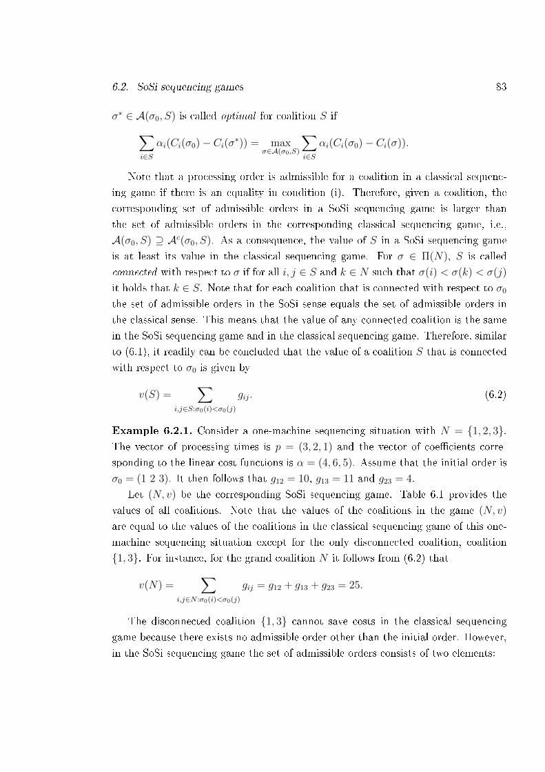
6.2. SoSi sequencing games 83
σ∗ ∈ A(σ0, S) is called optimal for coalition S if∑i∈S
αi(Ci(σ0)− Ci(σ∗)) = maxσ∈A(σ0,S)
∑i∈S
αi(Ci(σ0)− Ci(σ)).
Note that a processing order is admissible for a coalition in a classical sequenc-
ing game if there is an equality in condition (i). Therefore, given a coalition, the
corresponding set of admissible orders in a SoSi sequencing game is larger than
the set of admissible orders in the corresponding classical sequencing game, i.e.,
A(σ0, S) ⊇ Ac(σ0, S). As a consequence, the value of S in a SoSi sequencing game
is at least its value in the classical sequencing game. For σ ∈ Π(N), S is called
connected with respect to σ if for all i, j ∈ S and k ∈ N such that σ(i) < σ(k) < σ(j)
it holds that k ∈ S. Note that for each coalition that is connected with respect to σ0
the set of admissible orders in the SoSi sense equals the set of admissible orders in
the classical sense. This means that the value of any connected coalition is the same
in the SoSi sequencing game and in the classical sequencing game. Therefore, similar
to (6.1), it readily can be concluded that the value of a coalition S that is connected
with respect to σ0 is given by
v(S) =∑
i,j∈S:σ0(i)<σ0(j)
gij. (6.2)
Example 6.2.1. Consider a one-machine sequencing situation with N = 1, 2, 3.The vector of processing times is p = (3, 2, 1) and the vector of coecients corre-
sponding to the linear cost functions is α = (4, 6, 5). Assume that the initial order is
σ0 = (1 2 3). It then follows that g12 = 10, g13 = 11 and g23 = 4.
Let (N, v) be the corresponding SoSi sequencing game. Table 6.1 provides the
values of all coalitions. Note that the values of the coalitions in the game (N, v)
are equal to the values of the coalitions in the classical sequencing game of this one-
machine sequencing situation except for the only disconnected coalition, coalition
1, 3. For instance, for the grand coalition N it follows from (6.2) that
v(N) =∑
i,j∈N :σ0(i)<σ0(j)
gij = g12 + g13 + g23 = 25.
The disconnected coalition 1, 3 cannot save costs in the classical sequencing
game because there exists no admissible order other than the initial order. However,
in the SoSi sequencing game the set of admissible orders consists of two elements:
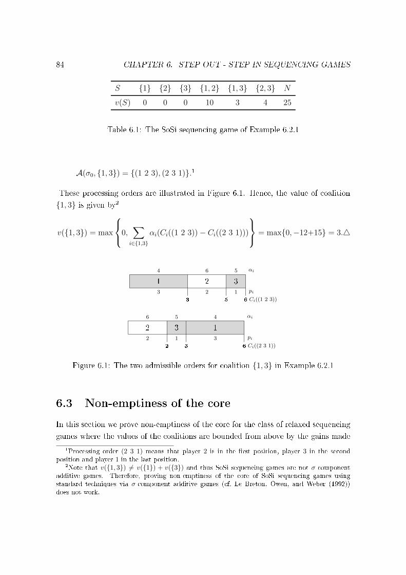
84 CHAPTER 6. STEP OUT - STEP IN SEQUENCING GAMES
S 1 2 3 1, 2 1, 3 2, 3 N
v(S) 0 0 0 10 3 4 25
Table 6.1: The SoSi sequencing game of Example 6.2.1
A(σ0, 1, 3) = (1 2 3), (2 3 1).1
These processing orders are illustrated in Figure 6.1. Hence, the value of coalition
1, 3 is given by2
v(1, 3) = max
0,∑i∈1,3
αi(Ci((1 2 3))− Ci((2 3 1)))
= max0,−12+15 = 3.4
1
4
3
3
2
6
2
5
3
5
1
6
αi
pi
Ci((1 2 3))
2
6
2
2
3
5
1
3
1
4
3
6
αi
pi
Ci((2 3 1))
Figure 6.1: The two admissible orders for coalition 1, 3 in Example 6.2.1
6.3 Non-emptiness of the core
In this section we prove non-emptiness of the core for the class of relaxed sequencing
games where the values of the coalitions are bounded from above by the gains made
1Processing order (2 3 1) means that player 2 is in the rst position, player 3 in the secondposition and player 1 in the last position.
2Note that v(1, 3) 6= v(1) + v(3) and thus SoSi sequencing games are not σ-componentadditive games. Therefore, proving non-emptiness of the core of SoSi sequencing games usingstandard techniques via σ-component additive games (cf. Le Breton, Owen, and Weber (1992))does not work.
6.3. Non-emptiness of the core 85
by all possible neighbor switches. Next, we show that the class of SoSi sequencing
games belongs to this class. As a consequence, every SoSi sequencing game has a
non-empty core.
Given an initial order σ0, assume that the set of admissible orders Ar(σ0, S) for
coalition S satises
Ac(σ0, S) ⊆ Ar(σ0, S),
for all S ⊆ N . Then, the corresponding relaxed sequencing game (N, v) is dened by
v(S) = maxσ∈Ar(σ0,S)
∑i∈S
αi(Ci(σ0)− Ci(σ)),
for all S ⊆ N . Note that a SoSi sequencing game indeed is a relaxed sequencing game
in the above sense. The following theorem proves that every connected marginal
vector is a core element for any relaxed sequencing game (N, v) where the value of a
coalition is bounded from above by the gains made by all possible neighbor switches,
i.e.,
v(S) ≤∑
i,j∈S:σ0(i)<σ0(j)
gij,
for all S ⊆ N . Notice that if a relaxed sequencing game (N, v) satises this condition,
then we have
v(S) =∑
i,j∈S:σ0(i)<σ0(j)
gij,
for every connected coalition S ⊆ N .
Theorem 6.3.1. Let (N, σ0, p, α) be a one-machine sequencing situation, let π ∈Π(N) be such that the set j ∈ N | π(j) ≤ π(i) is connected with respect to σ0 for
all i ∈ N and let (N, v) be a corresponding relaxed sequencing game such that
v(S) ≤∑
i,j∈S:σ0(i)<σ0(j)
gij, (6.3)
for all S ⊆ N . Then, mπ(v) ∈ C(v).
Proof. Let i ∈ N and denote Ti = j ∈ N | π(j) < π(i). Because π is connected it
follows that either Ti ⊆ P (σ0, i) or Ti ⊆ F (σ0, i) and therefore we have
mπi (v) = v(Ti ∪ i)− v(Ti)
86 CHAPTER 6. STEP OUT - STEP IN SEQUENCING GAMES
=∑
j,k∈Ti∪i:σ0(j)<σ0(k)
gjk −∑
j,k∈Ti:σ0(j)<σ0(k)
gjk
=
∑j∈Ti
gji if Ti ⊆ P (σ0, i)∑j∈Ti
gij if Ti ⊆ F (σ0, i),
where the second equality follows from the fact that the coalitions Ti and Ti∪i areconnected with respect to σ0.
Then, for S ⊆ N it holds that∑i∈S
mπi (v) =
∑i∈S:
Ti⊆P (σ0,i)
∑j∈Ti
gji +∑i∈S:
Ti⊆F (σ0,i)
∑j∈Ti
gij
≥∑i∈S:
Ti⊆P (σ0,i)
∑j∈Ti∩S
gji +∑i∈S:
Ti⊆F (σ0,i)
∑j∈Ti∩S
gij
=∑i∈S
∑j∈Ti∩S∩P (σ0,i)
gji +∑i∈S
∑j∈Ti∩S∩F (σ0,i)
gij
=∑j∈S
∑i∈S∩F (σ0,j):
i 6∈Tj
gji +∑i∈S
∑j∈Ti∩S∩F (σ0,i)
gij
=∑i∈S
∑j∈S∩F (σ0,i):
j 6∈Ti
gij +∑i∈S
∑j∈Ti∩S∩F (σ0,i)
gij
=∑i∈S
∑j∈S∩F (σ0,i)
gij
=∑
i,j∈S:σ0(i)<σ0(j)
gij
≥ v(S).
In the above derivation, the equations follow from
- interchanging the summations of the rst term and the fact that i ∈ Tj if and only
if j 6∈ Ti for all i, j ∈ N with i 6= j (third equality),
- interchanging the indices of the summations of the rst term (fourth equality).
Note that if S = N the inequalities become equalities. This proves that mπ(v) ∈C(v).
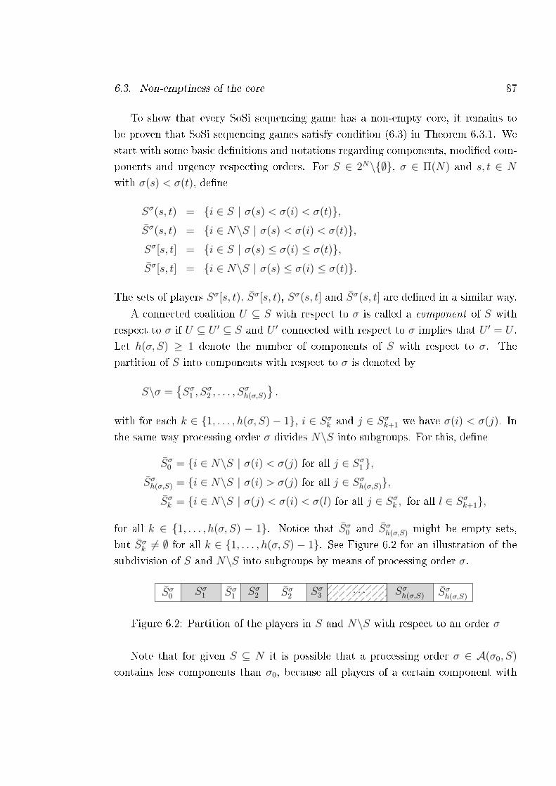
6.3. Non-emptiness of the core 87
To show that every SoSi sequencing game has a non-empty core, it remains to
be proven that SoSi sequencing games satisfy condition (6.3) in Theorem 6.3.1. We
start with some basic denitions and notations regarding components, modied com-
ponents and urgency respecting orders. For S ∈ 2N\∅, σ ∈ Π(N) and s, t ∈ N
with σ(s) < σ(t), dene
Sσ(s, t) = i ∈ S | σ(s) < σ(i) < σ(t),Sσ(s, t) = i ∈ N\S | σ(s) < σ(i) < σ(t),Sσ[s, t] = i ∈ S | σ(s) ≤ σ(i) ≤ σ(t),Sσ[s, t] = i ∈ N\S | σ(s) ≤ σ(i) ≤ σ(t).
The sets of players Sσ[s, t), Sσ[s, t), Sσ(s, t] and Sσ(s, t] are dened in a similar way.
A connected coalition U ⊆ S with respect to σ is called a component of S with
respect to σ if U ⊆ U ′ ⊆ S and U ′ connected with respect to σ implies that U ′ = U .
Let h(σ, S) ≥ 1 denote the number of components of S with respect to σ. The
partition of S into components with respect to σ is denoted by
S\σ =Sσ1 , S
σ2 , . . . , S
σh(σ,S)
.
with for each k ∈ 1, . . . , h(σ, S)− 1, i ∈ Sσk and j ∈ Sσk+1 we have σ(i) < σ(j). In
the same way processing order σ divides N\S into subgroups. For this, dene
Sσ0 = i ∈ N\S | σ(i) < σ(j) for all j ∈ Sσ1 ,Sσh(σ,S) = i ∈ N\S | σ(i) > σ(j) for all j ∈ Sσh(σ,S),
Sσk = i ∈ N\S | σ(j) < σ(i) < σ(l) for all j ∈ Sσk , for all l ∈ Sσk+1,
for all k ∈ 1, . . . , h(σ, S) − 1. Notice that Sσ0 and Sσh(σ,S) might be empty sets,
but Sσk 6= ∅ for all k ∈ 1, . . . , h(σ, S) − 1. See Figure 6.2 for an illustration of the
subdivision of S and N\S into subgroups by means of processing order σ.
Sσ0 Sσ1 Sσ1 Sσ2 Sσ2 Sσ3 . . . Sσh(σ,S) Sσh(σ,S)
Figure 6.2: Partition of the players in S and N\S with respect to an order σ
Note that for given S ⊆ N it is possible that a processing order σ ∈ A(σ0, S)
contains less components than σ0, because all players of a certain component with
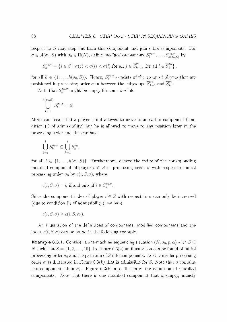
88 CHAPTER 6. STEP OUT - STEP IN SEQUENCING GAMES
respect to S may step out from this component and join other components. For
σ ∈ A(σ0, S) with σ0 ∈ Π(N), dene modied components Sσ0,σ1 , . . . , Sσ0,σh(σ0,S) by
Sσ0,σk =i ∈ S | σ(j) < σ(i) < σ(l) for all j ∈ Sσ0k−1, for all l ∈ S
σ0k
,
for all k ∈ 1, . . . , h(σ0, S). Hence, Sσ0,σk consists of the group of players that are
positioned in processing order σ in between the subgroups Sσ0k−1 and S
σ0k .
Note that Sσ0,σk might be empty for some k while
h(σ0,S)⋃k=1
Sσ0,σk = S.
Moreover, recall that a player is not allowed to move to an earlier component (con-
dition (i) of admissibility) but he is allowed to move to any position later in the
processing order and thus we have
l⋃k=1
Sσ0,σk ⊆l⋃
k=1
Sσ0k ,
for all l ∈ 1, . . . , h(σ0, S). Furthermore, denote the index of the corresponding
modied component of player i ∈ S in processing order σ with respect to initial
processing order σ0 by c(i, S, σ), where
c(i, S, σ) = k if and only if i ∈ Sσ0,σk .
Since the component index of player i ∈ S with respect to σ can only be increased
(due to condition (i) of admissibility), we have
c(i, S, σ) ≥ c(i, S, σ0).
An illustration of the denitions of components, modied components and the
index c(i, S, σ) can be found in the following example.
Example 6.3.1. Consider a one-machine sequencing situation (N, σ0, p, α) with S ⊆N such that S = 1, 2, . . . , 10. In Figure 6.3(a) an illustration can be found of initial
processing order σ0 and the partition of S into components. Next, consider processing
order σ as illustrated in Figure 6.3(b) that is admissible for S. Note that σ contains
less components than σ0. Figure 6.3(b) also illustrates the denition of modied
components. Note that there is one modied component that is empty, namely
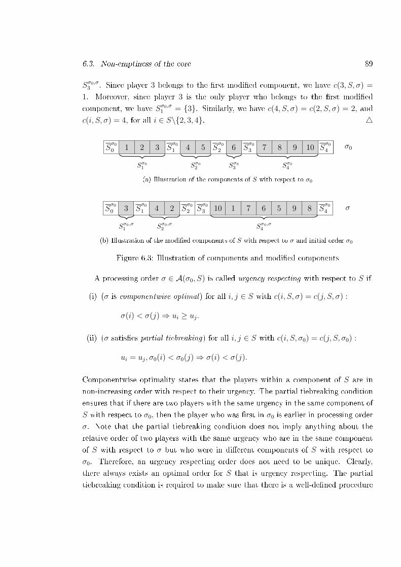
6.3. Non-emptiness of the core 89
Sσ0,σ3 . Since player 3 belongs to the rst modied component, we have c(3, S, σ) =
1. Moreover, since player 3 is the only player who belongs to the rst modied
component, we have Sσ0,σ1 = 3. Similarly, we have c(4, S, σ) = c(2, S, σ) = 2, and
c(i, S, σ) = 4, for all i ∈ S\2, 3, 4. 4
Sσ00 1 2 3 S
σ01 4 5 S
σ02 6 S
σ03 7 8 9 10 S
σ04
σ0
Sσ01 Sσ0
2 Sσ03 Sσ0
4
(a) Illustration of the components of S with respect to σ0
Sσ00 3 S
σ01 4 2 S
σ02 S
σ03 10 1 7 6 5 9 8 S
σ04
σ
Sσ0,σ1 Sσ0,σ
2 Sσ0,σ4
(b) Illustration of the modied components of S with respect to σ and initial order σ0
Figure 6.3: Illustration of components and modied components
A processing order σ ∈ A(σ0, S) is called urgency respecting with respect to S if
(i) (σ is componentwise optimal) for all i, j ∈ S with c(i, S, σ) = c(j, S, σ) :
σ(i) < σ(j)⇒ ui ≥ uj.
(ii) (σ satises partial tiebreaking) for all i, j ∈ S with c(i, S, σ0) = c(j, S, σ0) :
ui = uj, σ0(i) < σ0(j)⇒ σ(i) < σ(j).
Componentwise optimality states that the players within a component of S are in
non-increasing order with respect to their urgency. The partial tiebreaking condition
ensures that if there are two players with the same urgency in the same component of
S with respect to σ0, then the player who was rst in σ0 is earlier in processing order
σ. Note that the partial tiebreaking condition does not imply anything about the
relative order of two players with the same urgency who are in the same component
of S with respect to σ but who were in dierent components of S with respect to
σ0. Therefore, an urgency respecting order does not need to be unique. Clearly,
there always exists an optimal order for S that is urgency respecting. The partial
tiebreaking condition is required to make sure that there is a well-dened procedure
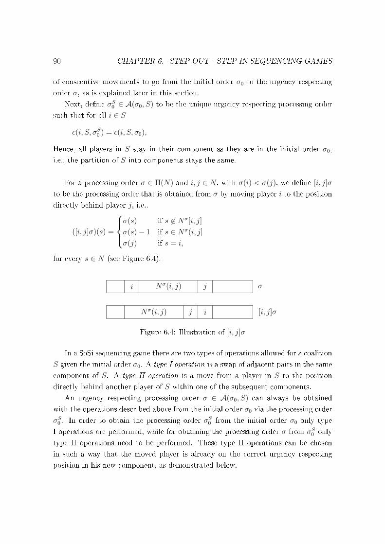
90 CHAPTER 6. STEP OUT - STEP IN SEQUENCING GAMES
of consecutive movements to go from the initial order σ0 to the urgency respecting
order σ, as is explained later in this section.
Next, dene σS0 ∈ A(σ0, S) to be the unique urgency respecting processing order
such that for all i ∈ S
c(i, S, σS0 ) = c(i, S, σ0),
Hence, all players in S stay in their component as they are in the initial order σ0,
i.e., the partition of S into components stays the same.
For a processing order σ ∈ Π(N) and i, j ∈ N , with σ(i) < σ(j), we dene [i, j]σ
to be the processing order that is obtained from σ by moving player i to the position
directly behind player j, i.e.,
([i, j]σ)(s) =
σ(s) if s 6∈ Nσ[i, j]
σ(s)− 1 if s ∈ Nσ(i, j]
σ(j) if s = i,
for every s ∈ N (see Figure 6.4).
i Nσ(i, j) j σ
Nσ(i, j) j i [i, j]σ
Figure 6.4: Illustration of [i, j]σ
In a SoSi sequencing game there are two types of operations allowed for a coalition
S given the initial order σ0. A type I operation is a swap of adjacent pairs in the same
component of S. A type II operation is a move from a player in S to the position
directly behind another player of S within one of the subsequent components.
An urgency respecting processing order σ ∈ A(σ0, S) can always be obtained
with the operations described above from the initial order σ0 via the processing order
σS0 . In order to obtain the processing order σS0 from the initial order σ0 only type
I operations are performed, while for obtaining the processing order σ from σS0 only
type II operations need to be performed. These type II operations can be chosen
in such a way that the moved player is already on the correct urgency respecting
position in his new component, as demonstrated below.
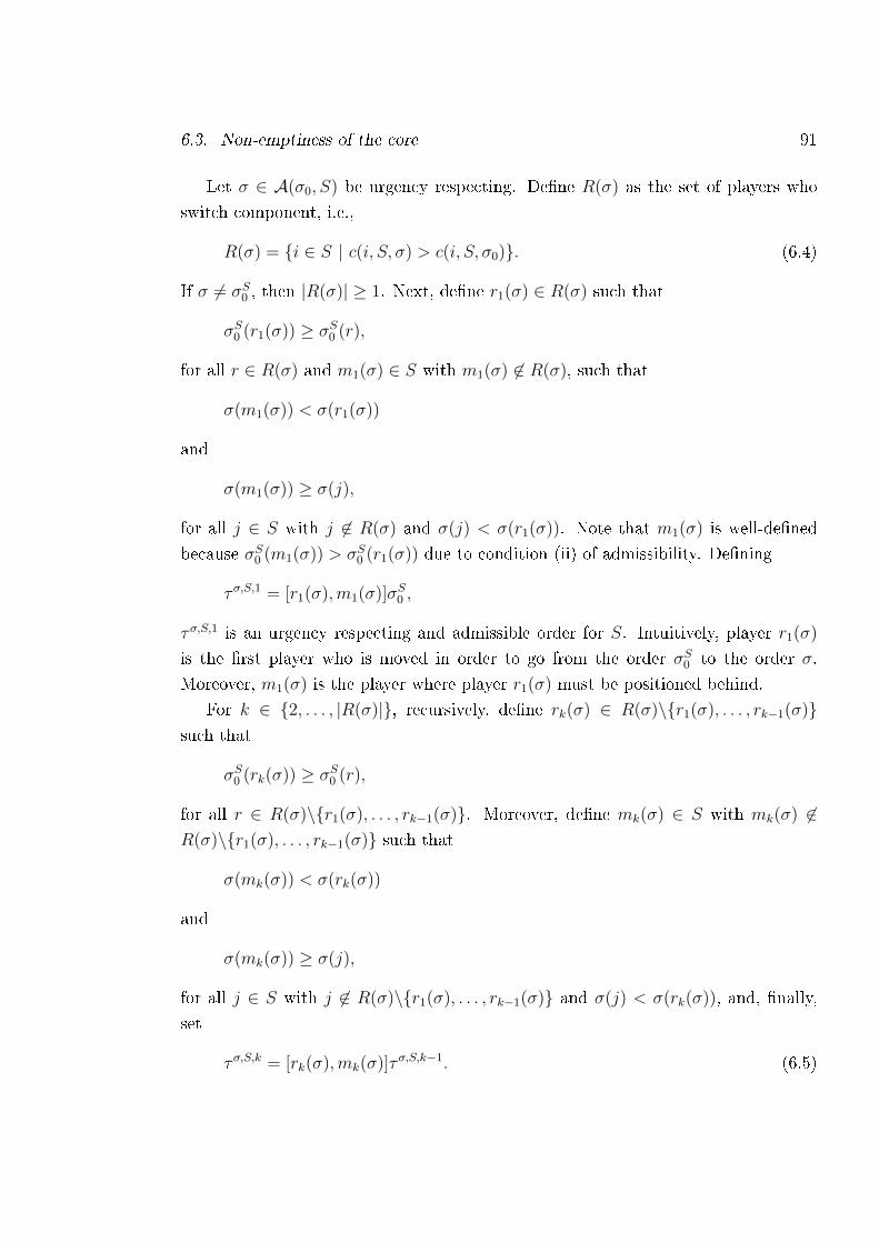
6.3. Non-emptiness of the core 91
Let σ ∈ A(σ0, S) be urgency respecting. Dene R(σ) as the set of players who
switch component, i.e.,
R(σ) = i ∈ S | c(i, S, σ) > c(i, S, σ0). (6.4)
If σ 6= σS0 , then |R(σ)| ≥ 1. Next, dene r1(σ) ∈ R(σ) such that
σS0 (r1(σ)) ≥ σS0 (r),
for all r ∈ R(σ) and m1(σ) ∈ S with m1(σ) 6∈ R(σ), such that
σ(m1(σ)) < σ(r1(σ))
and
σ(m1(σ)) ≥ σ(j),
for all j ∈ S with j 6∈ R(σ) and σ(j) < σ(r1(σ)). Note that m1(σ) is well-dened
because σS0 (m1(σ)) > σS0 (r1(σ)) due to condition (ii) of admissibility. Dening
τσ,S,1 = [r1(σ),m1(σ)]σS0 ,
τσ,S,1 is an urgency respecting and admissible order for S. Intuitively, player r1(σ)
is the rst player who is moved in order to go from the order σS0 to the order σ.
Moreover, m1(σ) is the player where player r1(σ) must be positioned behind.
For k ∈ 2, . . . , |R(σ)|, recursively, dene rk(σ) ∈ R(σ)\r1(σ), . . . , rk−1(σ)such that
σS0 (rk(σ)) ≥ σS0 (r),
for all r ∈ R(σ)\r1(σ), . . . , rk−1(σ). Moreover, dene mk(σ) ∈ S with mk(σ) 6∈R(σ)\r1(σ), . . . , rk−1(σ) such that
σ(mk(σ)) < σ(rk(σ))
and
σ(mk(σ)) ≥ σ(j),
for all j ∈ S with j 6∈ R(σ)\r1(σ), . . . , rk−1(σ) and σ(j) < σ(rk(σ)), and, nally,
set
τσ,S,k = [rk(σ),mk(σ)]τσ,S,k−1. (6.5)
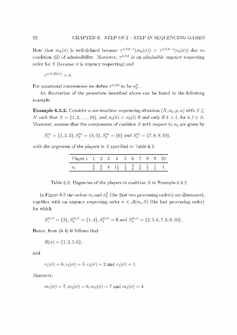
92 CHAPTER 6. STEP OUT - STEP IN SEQUENCING GAMES
Note that mk(σ) is well-dened because τσ,S,k−1(mk(σ)) > τσ,S,k−1(rk(σ)) due to
condition (ii) of admissibility. Moreover, τσ,S,k is an admissible urgency respecting
order for S (because σ is urgency respecting) and
τσ,S,|R(σ)| = σ.
For notational convenience we dene τσ,S,0 to be σS0 .
An illustration of the procedure described above can be found in the following
example.
Example 6.3.2. Consider a one-machine sequencing situation (N, σ0, p, α) with S ⊆N such that S = 1, 2, . . . , 10, and σ0(k) < σ0(l) if and only if k < l, for k, l ∈ S.Moreover, assume that the components of coalition S with respect to σ0 are given by
Sσ01 = 1, 2, 3, Sσ02 = 4, 5, Sσ03 = 6 and Sσ04 = 7, 8, 9, 10,
with the urgencies of the players in S specied in Table 6.2.
Player i 1 2 3 4 5 6 7 8 9 10
ui49
49
4 112
13
38
49
15
14
1
Table 6.2: Urgencies of the players in coalition S in Example 6.3.2
In Figure 6.5 the orders σ0 and σS0 (the rst two processing orders) are illustrated,
together with an urgency respecting order σ ∈ A(σ0, S) (the last processing order)
for which
Sσ0,σ1 = 3, Sσ0,σ2 = 1, 4, Sσ0,σ3 = ∅ and Sσ0,σ4 = 2, 5, 6, 7, 8, 9, 10.
Hence, from (6.4) it follows that
R(σ) = 1, 2, 5, 6,
and
r1(σ) = 6, r2(σ) = 5, r3(σ) = 2 and r4(σ) = 1.
Moreover,
m1(σ) = 7,m2(σ) = 6,m3(σ) = 7 and m4(σ) = 4.
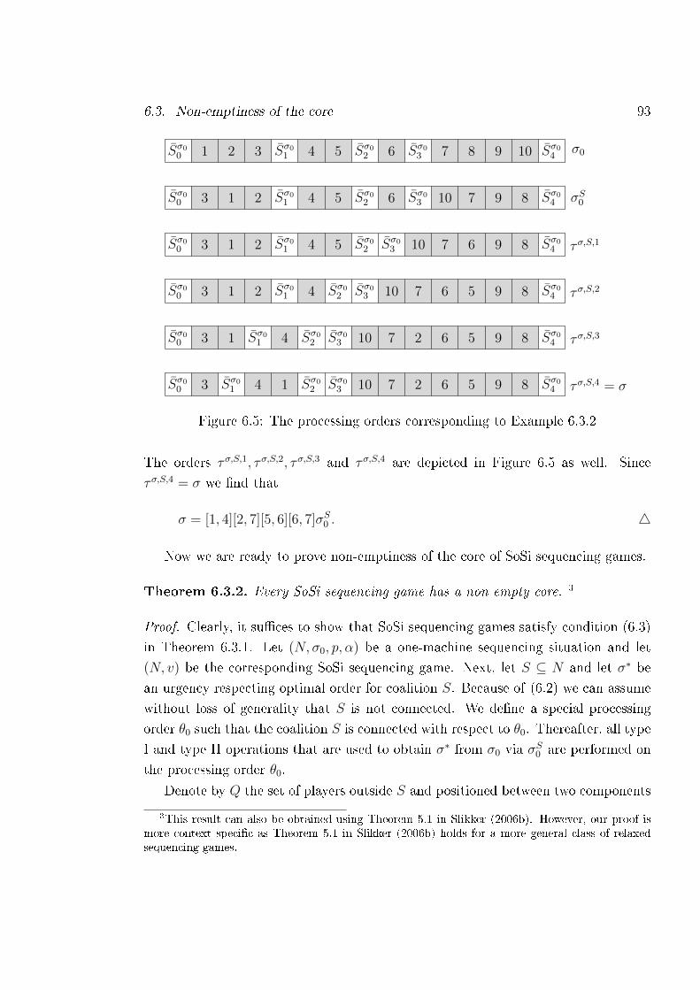
6.3. Non-emptiness of the core 93
Sσ00 1 2 3 Sσ01 4 5 Sσ02 6 Sσ03 7 8 9 10 Sσ04σ0
Sσ00 3 1 2 Sσ01 4 5 Sσ02 6 Sσ03 10 7 9 8 Sσ04 σS0
Sσ00 3 1 2 Sσ01 4 5 Sσ02 Sσ03 10 7 6 9 8 Sσ04 τσ,S,1
Sσ00 3 1 2 Sσ01 4 Sσ02 Sσ03 10 7 6 5 9 8 Sσ04 τσ,S,2
Sσ00 3 1 Sσ01 4 Sσ02 Sσ03 10 7 2 6 5 9 8 Sσ04 τσ,S,3
Sσ00 3 Sσ01 4 1 Sσ02 Sσ03 10 7 2 6 5 9 8 Sσ04 τσ,S,4 = σ
Figure 6.5: The processing orders corresponding to Example 6.3.2
The orders τσ,S,1, τσ,S,2, τσ,S,3 and τσ,S,4 are depicted in Figure 6.5 as well. Since
τσ,S,4 = σ we nd that
σ = [1, 4][2, 7][5, 6][6, 7]σS0 . 4
Now we are ready to prove non-emptiness of the core of SoSi sequencing games.
Theorem 6.3.2. Every SoSi sequencing game has a non-empty core. 3
Proof. Clearly, it suces to show that SoSi sequencing games satisfy condition (6.3)
in Theorem 6.3.1. Let (N, σ0, p, α) be a one-machine sequencing situation and let
(N, v) be the corresponding SoSi sequencing game. Next, let S ⊆ N and let σ∗ be
an urgency respecting optimal order for coalition S. Because of (6.2) we can assume
without loss of generality that S is not connected. We dene a special processing
order θ0 such that the coalition S is connected with respect to θ0. Thereafter, all type
I and type II operations that are used to obtain σ∗ from σ0 via σS0 are performed on
the processing order θ0.
Denote by Q the set of players outside S and positioned between two components
3This result can also be obtained using Theorem 5.1 in Slikker (2006b). However, our proof ismore context specic as Theorem 5.1 in Slikker (2006b) holds for a more general class of relaxedsequencing games.
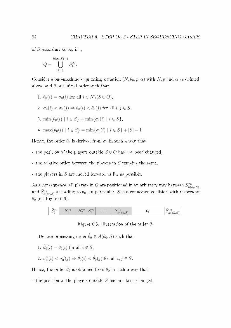
94 CHAPTER 6. STEP OUT - STEP IN SEQUENCING GAMES
of S according to σ0, i.e.,
Q =
h(σ0,S)−1⋃k=1
Sσ0k .
Consider a one-machine sequencing situation (N, θ0, p, α) with N, p and α as dened
above and θ0 an initial order such that
1. θ0(i) = σ0(i) for all i ∈ N\(S ∪Q),
2. σ0(i) < σ0(j)⇒ θ0(i) < θ0(j) for all i, j ∈ S,
3. minθ0(i) | i ∈ S = minσ0(i) | i ∈ S,
4. maxθ0(i) | i ∈ S = minσ0(i) | i ∈ S+ |S| − 1.
Hence, the order θ0 is derived from σ0 in such a way that
- the position of the players outside S ∪Q has not been changed,
- the relative order between the players in S remains the same,
- the players in S are moved forward as far as possible.
As a consequence, all players in Q are positioned in an arbitrary way between Sσ0h(σ0,S)
and Sσ0h(σ0,S) according to θ0. In particular, S is a connected coalition with respect to
θ0 (cf. Figure 6.6).
Sσ00 Sσ01 Sσ02 Sσ03. . . Sσ0h(σ0,S) Q Sσ0h(σ0,S)
Figure 6.6: Illustration of the order θ0
Denote processing order θ0 ∈ A(θ0, S) such that
1. θ0(i) = θ0(i) for all i 6∈ S,
2. σS0 (i) < σS0 (j)⇒ θ0(i) < θ0(j) for all i, j ∈ S.
Hence, the order θ0 is obtained from θ0 in such a way that
- the position of the players outside S has not been changed,
6.3. Non-emptiness of the core 95
- such that the relative order between the players in S is the same as their relative
order in σS0 .
Obviously θ0 can be obtained from θ0 in exactly the same way as σS0 from σ0 using
the same operations of type I, conducted in the same order. Note that each operation
results in the same cost dierence. Therefore,∑i∈S
αi(Ci(σ0)− Ci(σS0 )) =∑i∈S
αi(Ci(θ0)− Ci(θ0)). (6.6)
Observe that if the order σ0 is already urgency respecting, i.e., if σS0 = σ0, then also
θ0 = θ0 and thus (6.6) still holds.
Next, let R = R(σ∗), rk = rk(σ∗) and mk = mk(σ
∗) for all k ∈ 1, . . . , |R| asdened in (6.4) such that
σ∗ = [r|R|,m|R|] . . . [r2,m2][r1,m1]σS0 .
Dene the processing order θ∗ by
θ∗ = [r|R|,m|R|] . . . [r2,m2][r1,m1]θ0.
Remember, if |R| = 0, then σ∗ = σS0 and thus also θ∗ = θ0. The processing order θ∗
is obtained from θ0 in the same way as σ∗ is obtained from σS0 using the same type
II operations, conducted in the same order. Note that these operations are indeed
valid due to the denition of θ0. Obviously, θ∗ is an admissible order for S in the
sequencing situation (N, θ0, p, α). Abbreviate τσ∗,S,k for k ∈ 0, 1, . . . , |R| as dened
in (6.5) by σk. Moreover, set
θk = [rk,mk] . . . [r2,m2][r1,m1]θ0,
for all k ∈ 0, 1, . . . , |R|. Notice that θ|R| = θ∗.
Let k ∈ 1, . . . , |R| and consider the operation [rk,mk] performed on σk−1 and
θk−1. Then,∑i∈S
αi(Ci(σk−1)− Ci(σk)) =
∑i∈Sσk−1 (rk,mk]
αi
prk − αrk
∑i∈N σk−1 (rk,mk]
pi
≤
∑i∈Sσk−1 (rk,mk]
αi
prk − αrk
∑i∈Sσk−1 (rk,mk]
pi
96 CHAPTER 6. STEP OUT - STEP IN SEQUENCING GAMES
=
∑i∈Sθk−1 (rk,mk]
αi
prk − αrk
∑i∈Sθk−1 (rk,mk]
pi
=
∑i∈S
αi(Ci(θk−1)− Ci(θk)).
Hence,
v(S) =∑i∈S
αi(Ci(σ0)− Ci(σ∗))
=∑i∈S
αi(Ci(σ0)− Ci(σS0 )) +
|R|∑k=1
∑i∈S
αi(Ci(σk−1)− Ci(σk))
≤∑i∈S
αi(Ci(θ0)− Ci(θ0)) +
|R|∑k=1
∑i∈S
αi(Ci(θk−1)− Ci(θk))
=∑i∈S
αi(Ci(θ0)− Ci(θ∗))
≤ maxθ∈A(θ0,S)
∑i∈S
αi(Ci(θ0)− Ci(θ))
=∑
i,j∈S:θ0(i)<θ0(j)
gij
=∑
i,j∈S:σ0(i)<σ0(j)
gij,
also if |R| = 0. In the above derivation, the last two equalities follow from
- the fact that coalition S is connected with respect to θ0,
- the fact that the relative order of the players in S with respect to θ0 is the same as
the relative order of the players in S with respect to σ0.
6.4 A polynomial time algorithm for each coalition
This section provides a polynomial time algorithm determining an optimal order for
every possible coalition and, consequently, the values of the coalitions. First, some
new notions as composed costs per time unit, composed processing times and com-
posed urgencies are introduced. Using these notions we can exclude some admissible
orders from being optimal.
6.4. A polynomial time algorithm for each coalition 97
The composed costs per time unit αS and the composed processing time pS for a
coalition S ∈ 2N are dened by
αS =∑i∈S
αi
and
pS =∑i∈S
pi,
respectively. Consequently, the composed urgency uS of a non-empty coalition S ∈2N\∅ is dened by
uS =αSpS.
Next we explain how the concept of composed urgency helps to decide which of
two related processing orders is less costly for a certain coalition. For the moment we
do not worry about admissibility of these orders. Consider a non-empty coalition S
and a processing order σ ∈ Π(N). First take i ∈ S and j ∈ N such that σ(i) < σ(j).
Let σ ∈ Π(N) be the processing order obtained from σ by moving player i to the
position directly behind player j. Then the dierence between the costs for coalition
S with respect to the processing order σ and the processing order σ can be calculated
as follows: ∑s∈S
αsCs(σ)−∑s∈S
αsCs(σ)
=∑
s∈Sσ(i,j]
αspi − αi∑
s∈Nσ(i,j]
ps
= αSσ(i,j]pi − αipNσ(i,j].
Similarly, take i ∈ S and j ∈ N such that σ(i) > σ(j) and let σ ∈ Π(N) be the
processing order obtained from σ by moving player i to the position directly in front
of player j. Then the dierence between the costs for coalition S with respect to
processing order σ and processing order σ is equal to
αipNσ [j,i) − αSσ [j,i)pi.
Hence, with δσi (j, S) representing the cost dierence for coalition S made by moving
player i directly behind player j in case σ(i) < σ(j) and the cost dierence made by
98 CHAPTER 6. STEP OUT - STEP IN SEQUENCING GAMES
moving player i directly in front of player j in case σ(i) > σ(j), we have
δσi (j, S) =
αSσ(i,j]pi − αipNσ(i,j] if σ(i) < σ(j)
αipNσ [j,i) − αSσ [j,i)pi if σ(i) > σ(j),(6.7)
for all i ∈ S and j ∈ N .
The above cost dierences have an additive structure in the following sense. Take
i ∈ S and j, k ∈ N such that σ(i) < σ(j) < σ(k). The cost dierence δσi (k, S) can be
split up in two parts by rst moving player i to the position directly behind player
j and thereafter moving player i to the position directly behind player k. Hence, we
can write
δσi (k, S) = δσi (j, S) + δσi (k, S),
where σ ∈ Π(N) is the processing order obtained from σ by moving player i to the
position directly behind player j.
Using the above notation of a cost dierence it is easily checked whether having
a certain player i ∈ S in a later position (behind player j) in the processing order is
benecial for S or not because
δσi (j, S) > 0 ⇔ αipi<αSσ(i,j]
pNσ(i,j]
,
δσi (j, S) = 0 ⇔ αipi
=αSσ(i,j]
pNσ(i,j]
,
δσi (j, S) < 0 ⇔ αipi>αSσ(i,j]
pNσ(i,j]
,
with σ(i) < σ(j). Similarly, it is also easily checked whether having a certain player
i ∈ S on a position earlier (in front of player j) in the processing order is benecial
for S or not because
δσi (j, S) > 0 ⇔ αipi>αSσ [j,i)
pNσ [j,i)
,
δσi (j, S) = 0 ⇔ αipi
=αSσ [j,i)
pNσ [j,i)
,
δσi (j, S) < 0 ⇔ αipi<αSσ [j,i)
pNσ [j,i)
,
with σ(i) > σ(j).
Using these criteria one can exclude some admissible orders from being optimal,
as illustrated in the following lemma. To be specic, Lemma 6.4.1 states that if
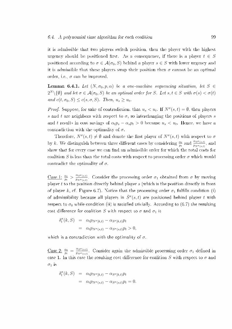
6.4. A polynomial time algorithm for each coalition 99
it is admissible that two players switch position, then the player with the highest
urgency should be positioned rst. As a consequence, if there is a player t ∈ S
positioned according to σ ∈ A(σ0, S) behind a player s ∈ S with lower urgency and
it is admissible that these players swap their position then σ cannot be an optimal
order, i.e., σ can be improved.
Lemma 6.4.1. Let (N, σ0, p, α) be a one-machine sequencing situation, let S ∈2N\∅ and let σ ∈ A(σ0, S) be an optimal order for S. Let s, t ∈ S with σ(s) < σ(t)
and c(t, σ0, S) ≤ c(s, σ, S). Then, us ≥ ut.
Proof. Suppose, for sake of contradiction, that us < ut. If Nσ(s, t) = ∅, then players
s and t are neighbors with respect to σ, so interchanging the positions of players s
and t results in cost savings of αtps − αspt > 0 because us < ut. Hence, we have a
contradiction with the optimality of σ.
Therefore, Nσ(s, t) 6= ∅ and denote the rst player of Nσ(s, t) with respect to σ
by k. We distinguish between three dierent cases by considering αtpt
andαSσ(s,t)
pNσ(s,t), and
show that for every case we can nd an admissible order for which the total costs for
coalition S is less than the total costs with respect to processing order σ which would
contradict the optimality of σ.
Case 1: αtpt>
αSσ(s,t)
pNσ(s,t). Consider the processing order σ1 obtained from σ by moving
player t to the position directly behind player s (which is the position directly in front
of player k, cf. Figure 6.7). Notice that the processing order σ1 fullls condition (i)
of admissibility because all players in Sσ(s, t) are positioned behind player t with
respect to σ0 while condition (ii) is satised trivially. According to (6.7) the resulting
cost dierence for coalition S with respect to σ and σ1 is
δσt (k, S) = αtpNσ [k,t) − αSσ [k,t)pt
= αtpNσ(s,t) − αSσ(s,t)pt > 0,
which is a contradiction with the optimality of σ.
Case 2: αtpt
=αSσ(s,t)
pNσ(s,t). Consider again the admissible processing order σ1 dened in
case 1. In this case the resulting cost dierence for coalition S with respect to σ and
σ1 is
δσt (k, S) = αtpNσ [k,t) − αSσ [k,t)pt
= αtpNσ(s,t) − αSσ(s,t)pt = 0.
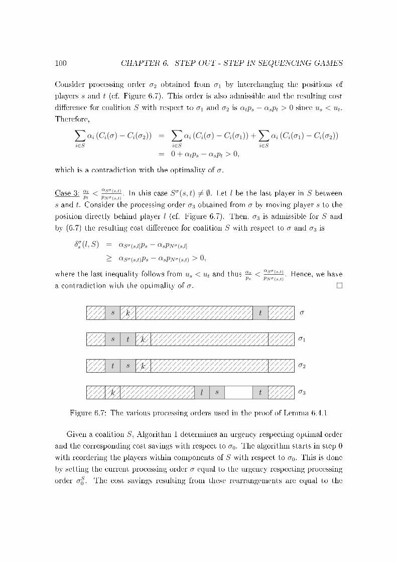
100 CHAPTER 6. STEP OUT - STEP IN SEQUENCING GAMES
Consider processing order σ2 obtained from σ1 by interchanging the positions of
players s and t (cf. Figure 6.7). This order is also admissible and the resulting cost
dierence for coalition S with respect to σ1 and σ2 is αtps − αspt > 0 since us < ut.
Therefore,∑i∈S
αi (Ci(σ)− Ci(σ2)) =∑i∈S
αi (Ci(σ)− Ci(σ1)) +∑i∈S
αi (Ci(σ1)− Ci(σ2))
= 0 + αtps − αspt > 0,
which is a contradiction with the optimality of σ.
Case 3: αtpt<
αSσ(s,t)
pNσ(s,t). In this case Sσ(s, t) 6= ∅. Let l be the last player in S between
s and t. Consider the processing order σ3 obtained from σ by moving player s to the
position directly behind player l (cf. Figure 6.7). Then, σ3 is admissible for S and
by (6.7) the resulting cost dierence for coalition S with respect to σ and σ3 is
δσs (l, S) = αSσ(s,l]ps − αspNσ(s,l]
≥ αSσ(s,t)ps − αspNσ(s,t) > 0,
where the last inequality follows from us < ut and thus αsps<
αSσ(s,t)
pNσ(s,t). Hence, we have
a contradiction with the optimality of σ.
s k t σ
s t k σ1
t s k σ2
k l s t σ3
Figure 6.7: The various processing orders used in the proof of Lemma 6.4.1
Given a coalition S, Algorithm 1 determines an urgency respecting optimal order
and the corresponding cost savings with respect to σ0. The algorithm starts in step 0
with reordering the players within components of S with respect to σ0. This is done
by setting the current processing order σ equal to the urgency respecting processing
order σS0 . The cost savings resulting from these rearrangements are equal to the
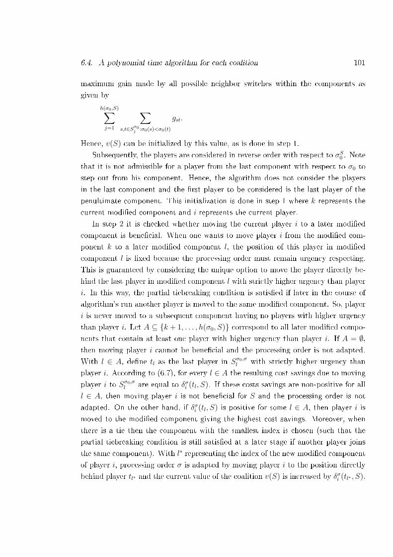
6.4. A polynomial time algorithm for each coalition 101
maximum gain made by all possible neighbor switches within the components as
given by
h(σ0,S)∑j=1
∑s,t∈Sσ0j :σ0(s)<σ0(t)
gst.
Hence, v(S) can be initialized by this value, as is done in step 1.
Subsequently, the players are considered in reverse order with respect to σS0 . Note
that it is not admissible for a player from the last component with respect to σ0 to
step out from his component. Hence, the algorithm does not consider the players
in the last component and the rst player to be considered is the last player of the
penultimate component. This initialization is done in step 1 where k represents the
current modied component and i represents the current player.
In step 2 it is checked whether moving the current player i to a later modied
component is benecial. When one wants to move player i from the modied com-
ponent k to a later modied component l, the position of this player in modied
component l is xed because the processing order must remain urgency respecting.
This is guaranteed by considering the unique option to move the player directly be-
hind the last player in modied component l with strictly higher urgency than player
i. In this way, the partial tiebreaking condition is satised if later in the course of
algorithm's run another player is moved to the same modied component. So, player
i is never moved to a subsequent component having no players with higher urgency
than player i. Let A ⊆ k + 1, . . . , h(σ0, S) correspond to all later modied compo-
nents that contain at least one player with higher urgency than player i. If A = ∅,then moving player i cannot be benecial and the processing order is not adapted.
With l ∈ A, dene tl as the last player in Sσ0,σl with strictly higher urgency than
player i. According to (6.7), for every l ∈ A the resulting cost savings due to moving
player i to Sσ0,σl are equal to δσi (tl, S). If these costs savings are non-positive for all
l ∈ A, then moving player i is not benecial for S and the processing order is not
adapted. On the other hand, if δσi (tl, S) is positive for some l ∈ A, then player i is
moved to the modied component giving the highest cost savings. Moreover, when
there is a tie then the component with the smallest index is chosen (such that the
partial tiebreaking condition is still satised at a later stage if another player joins
the same component). With l∗ representing the index of the new modied component
of player i, processing order σ is adapted by moving player i to the position directly
behind player tl∗ and the current value of the coalition v(S) is increased by δσi (tl∗ , S).
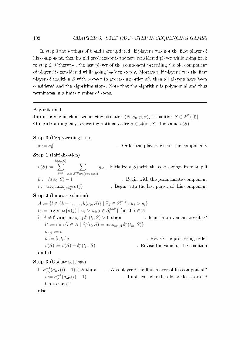
102 CHAPTER 6. STEP OUT - STEP IN SEQUENCING GAMES
In step 3 the settings of k and i are updated. If player i was not the rst player of
his component, then his old predecessor is the new considered player while going back
to step 2. Otherwise, the last player of the component preceding the old component
of player i is considered while going back to step 2. Moreover, if player i was the rst
player of coalition S with respect to processing order σS0 , then all players have been
considered and the algorithm stops. Note that the algorithm is polynomial and thus
terminates in a nite number of steps.
Algorithm 1
Input: a one-machine sequencing situation (N, σ0, p, α), a coalition S ∈ 2N\∅Output: an urgency respecting optimal order σ ∈ A(σ0, S), the value v(S)
Step 0 (Preprocessing step)
σ := σS0 . Order the players within the components
Step 1 (Initialization)
v(S) :=
h(σ0,S)∑j=1
∑s,t∈Sσ0j :σ0(s)<σ0(t)
gst . Initialize v(S) with the cost savings from step 0
k := h(σ0, S)− 1 . Begin with the penultimate component
i := arg maxj∈Sσ0k σ(j) . Begin with the last player of this component
Step 2 (Improve solution)
A := l ∈ k + 1, . . . , h(σ0, S) | ∃j ∈ Sσ0,σl : uj > uitl := arg maxσ(j) | uj > ui, j ∈ Sσ0,σl for all l ∈ Aif A 6= ∅ and maxl∈A δ
σi (tl, S) > 0 then . Is an improvement possible?
l∗ := min l ∈ A | δσi (tl, S) = maxm∈A δσi (tm, S)
σold := σ
σ := [i, tl∗ ]σ . Revise the processing order
v(S) := v(S) + δσi (tl∗ , S) . Revise the value of the coalition
end if
Step 3 (Update settings)
if σ−1old(σold(i)− 1) ∈ S then . Was player i the rst player of his component?
i := σ−1old(σold(i)− 1) . If not, consider the old predecessor of i
Go to step 2
else
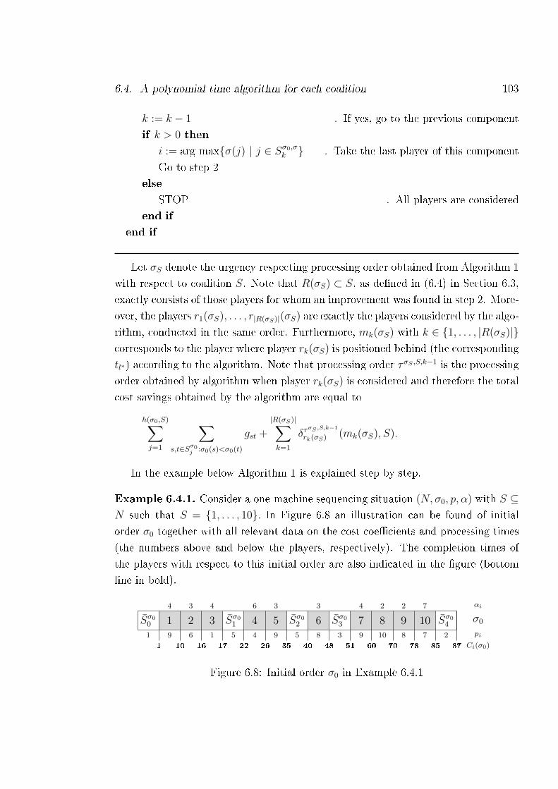
6.4. A polynomial time algorithm for each coalition 103
k := k − 1 . If yes, go to the previous component
if k > 0 then
i := arg maxσ(j) | j ∈ Sσ0,σk . Take the last player of this component
Go to step 2
else
STOP . All players are considered
end if
end if
Let σS denote the urgency respecting processing order obtained from Algorithm 1
with respect to coalition S. Note that R(σS) ⊂ S, as dened in (6.4) in Section 6.3,
exactly consists of those players for whom an improvement was found in step 2. More-
over, the players r1(σS), . . . , r|R(σS)|(σS) are exactly the players considered by the algo-
rithm, conducted in the same order. Furthermore, mk(σS) with k ∈ 1, . . . , |R(σS)|corresponds to the player where player rk(σS) is positioned behind (the corresponding
tl∗) according to the algorithm. Note that processing order τσS ,S,k−1 is the processing
order obtained by algorithm when player rk(σS) is considered and therefore the total
cost savings obtained by the algorithm are equal to
h(σ0,S)∑j=1
∑s,t∈Sσ0j :σ0(s)<σ0(t)
gst +
|R(σS)|∑k=1
δτσS,S,k−1
rk(σS) (mk(σS), S).
In the example below Algorithm 1 is explained step by step.
Example 6.4.1. Consider a one-machine sequencing situation (N, σ0, p, α) with S ⊆N such that S = 1, . . . , 10. In Figure 6.8 an illustration can be found of initial
order σ0 together with all relevant data on the cost coecients and processing times
(the numbers above and below the players, respectively). The completion times of
the players with respect to this initial order are also indicated in the gure (bottom
line in bold).
Sσ00
1
1
1
4
9
10
2
3
6
16
3
4
1
17
Sσ01
5
22
4
6
4
26
5
3
9
35
Sσ02
5
40
6
3
8
48
Sσ03
3
51
7
4
9
60
8
2
10
70
9
2
8
78
10
7
7
85
Sσ04
2
87
αi
σ0
pi
Ci(σ0)
Figure 6.8: Initial order σ0 in Example 6.4.1
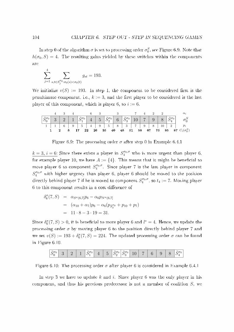
104 CHAPTER 6. STEP OUT - STEP IN SEQUENCING GAMES
In step 0 of the algorithm σ is set to processing order σS0 , see Figure 6.9. Note that
h(σ0, S) = 4. The resulting gains yielded by these switches within the components
are4∑j=1
∑s,t∈Sσ0j :σ0(s)<σ0(t)
gst = 193.
We initialize v(S) := 193. In step 1, the component to be considered rst is the
penultimate component, i.e., k := 3, and the rst player to be considered is the last
player of this component, which is player 6, so i := 6.
Sσ00
1
1
3
4
1
2
2
3
6
8
1
4
9
17
Sσ01
5
22
4
6
4
26
5
3
9
35
Sσ02
5
40
6
3
8
48
Sσ03
3
51
10
7
7
58
7
4
9
67
9
2
8
75
8
2
10
85
Sσ04
2
87
σS0
αi
pi
Ci(σS0 )
Figure 6.9: The processing order σ after step 0 in Example 6.4.1
k = 3, i = 6: Since there exists a player in Sσ0,σ4 who is more urgent than player 6,
for example player 10, we have A := 4. This means that it might be benecial to
move player 6 to component Sσ0,σ4 . Since player 7 is the last player in component
Sσ0,σ4 with higher urgency than player 6, player 6 should be moved to the position
directly behind player 7 if he is moved to component Sσ0,σ4 , so t4 := 7. Moving player
6 to this component results in a cost dierence of
δσ6 (7, S) = αSσ(6,7]p6 − α6pNσ(6,7]
= (α10 + α7)p6 − α6(pSσ03+ p10 + p7)
= 11 · 8− 3 · 19 = 31.
Since δσ6 (7, S) > 0, it is benecial to move player 6 and l∗ = 4. Hence, we update the
processing order σ by moving player 6 to the position directly behind player 7 and
we set v(S) := 193 + δσ6 (7, S) = 224. The updated processing order σ can be found
in Figure 6.10.
Sσ00 3 2 1 Sσ01 4 5 Sσ02 Sσ03 10 7 6 9 8 Sσ04
Figure 6.10: The processing order σ after player 6 is considered in Example 6.4.1
In step 3 we have to update k and i. Since player 6 was the only player in his
component, and thus his previous predecessor is not a member of coalition S, we
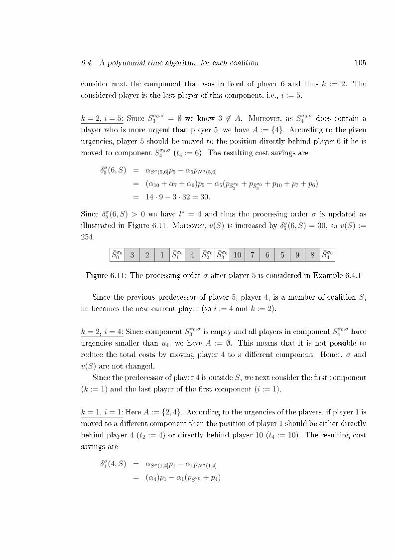
6.4. A polynomial time algorithm for each coalition 105
consider next the component that was in front of player 6 and thus k := 2. The
considered player is the last player of this component, i.e., i := 5.
k = 2, i = 5: Since Sσ0,σ3 = ∅ we know 3 6∈ A. Moreover, as Sσ0,σ4 does contain a
player who is more urgent than player 5, we have A := 4. According to the given
urgencies, player 5 should be moved to the position directly behind player 6 if he is
moved to component Sσ0,σ4 (t4 := 6). The resulting cost savings are
δσ5 (6, S) = αSσ(5,6]p5 − α5pNσ(5,6]
= (α10 + α7 + α6)p5 − α5(pSσ02+ pSσ03
+ p10 + p7 + p6)
= 14 · 9− 3 · 32 = 30.
Since δσ5 (6, S) > 0 we have l∗ = 4 and thus the processing order σ is updated as
illustrated in Figure 6.11. Moreover, v(S) is increased by δσ5 (6, S) = 30, so v(S) :=
254.
Sσ00 3 2 1 Sσ01 4 Sσ02 Sσ03 10 7 6 5 9 8 Sσ04
Figure 6.11: The processing order σ after player 5 is considered in Example 6.4.1
Since the previous predecessor of player 5, player 4, is a member of coalition S,
he becomes the new current player (so i := 4 and k := 2).
k = 2, i = 4: Since component Sσ0,σ3 is empty and all players in component Sσ0,σ4 have
urgencies smaller than u4, we have A := ∅. This means that it is not possible to
reduce the total costs by moving player 4 to a dierent component. Hence, σ and
v(S) are not changed.
Since the predecessor of player 4 is outside S, we next consider the rst component
(k := 1) and the last player of the rst component (i := 1).
k = 1, i = 1: Here A := 2, 4. According to the urgencies of the players, if player 1 is
moved to a dierent component then the position of player 1 should be either directly
behind player 4 (t2 := 4) or directly behind player 10 (t4 := 10). The resulting cost
savings are
δσ1 (4, S) = αSσ(1,4]p1 − α1pNσ(1,4]
= (α4)p1 − α1(pSσ01+ p4)
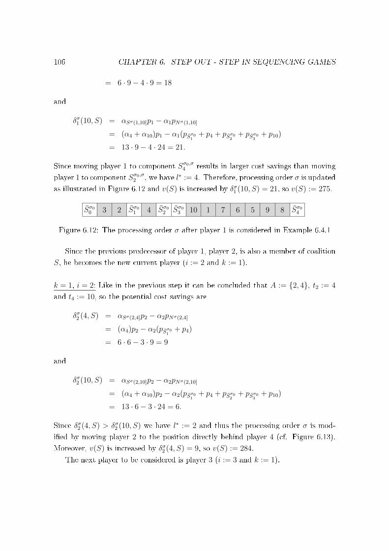
106 CHAPTER 6. STEP OUT - STEP IN SEQUENCING GAMES
= 6 · 9− 4 · 9 = 18
and
δσ1 (10, S) = αSσ(1,10]p1 − α1pNσ(1,10]
= (α4 + α10)p1 − α1(pSσ01+ p4 + pSσ02
+ pSσ03+ p10)
= 13 · 9− 4 · 24 = 21.
Since moving player 1 to component Sσ0,σ4 results in larger cost savings than moving
player 1 to component Sσ0,σ2 , we have l∗ := 4. Therefore, processing order σ is updated
as illustrated in Figure 6.12 and v(S) is increased by δσ1 (10, S) = 21, so v(S) := 275.
Sσ00 3 2 Sσ01 4 Sσ02 Sσ03 10 1 7 6 5 9 8 Sσ04
Figure 6.12: The processing order σ after player 1 is considered in Example 6.4.1
Since the previous predecessor of player 1, player 2, is also a member of coalition
S, he becomes the new current player (i := 2 and k := 1).
k = 1, i = 2: Like in the previous step it can be concluded that A := 2, 4, t2 := 4
and t4 := 10, so the potential cost savings are
δσ2 (4, S) = αSσ(2,4]p2 − α2pNσ(2,4]
= (α4)p2 − α2(pSσ01+ p4)
= 6 · 6− 3 · 9 = 9
and
δσ2 (10, S) = αSσ(2,10]p2 − α2pNσ(2,10]
= (α4 + α10)p2 − α2(pSσ01+ p4 + pSσ02
+ pSσ03+ p10)
= 13 · 6− 3 · 24 = 6.
Since δσ2 (4, S) > δσ2 (10, S) we have l∗ := 2 and thus the processing order σ is mod-
ied by moving player 2 to the position directly behind player 4 (cf. Figure 6.13).
Moreover, v(S) is increased by δσ2 (4, S) = 9, so v(S) := 284.
The next player to be considered is player 3 (i := 3 and k := 1).
6.4. A polynomial time algorithm for each coalition 107
Sσ00 3 Sσ01 4 2 Sσ02 Sσ03 10 1 7 6 5 9 8 Sσ04
Figure 6.13: The processing order σ after player 2 is considered in Example 6.4.1
k = 1, i = 3: Since all players in the components Sσ0,σ2 and Sσ0,σ4 have urgency smaller
than u3, we have A := ∅. Hence, σ and v(S) are not changed.
Next k := 0. According to step 4, the algorithm terminates and an optimal order
for coalition S is found, namely the processing order in Figure 6.13 which can be
summarized as
σS = [2, 4][1, 10][5, 6][6, 7]σS0 .
Moreover, the total cost savings obtained are 284. 4 4
The following lemma shows that Algorithm 1 always constructs an urgency re-
specting admissible order for a certain coalition S. This lemma is used to prove that
the processing order found by the algorithm is also optimal with respect to coalition
S (see Theorem 6.4.3).
Lemma 6.4.2. Let (N, σ0, p, α) be a one-machine sequencing situation and let S ∈2N\∅. Then Algorithm 1 constructs an urgency respecting admissible order σS for
coalition S.
Proof. We only have to prove that σS satises the partial tiebreaking condition, be-
cause the other conditions of admissibility and componentwise optimality are satised
trivially by construction. Suppose, for sake of contradiction, that σS does not sat-
isfy the partial tiebreaking condition. Then there exist i, j ∈ S with c(i, S, σ0) =
c(j, S, σ0), ui = uj, σ0(i) < σ0(j), while σS(i) > σS(j). Without loss of generality we
can assume σS0 (j) = σS0 (i) + 1. Let σj be the order obtained during the run of the
algorithm just before player j is considered and σi be the order obtained during the
run of the algorithm just before player i is considered, i.e., immediately after player
j is considered. We distinguish between two cases: σj = σi and σj 6= σi.
Case 1: σj = σi, i.e., player j has not been moved by the algorithm. Then, due to
the structure of the algorithm, there is a player t ∈ S with c(t, S, σi) > c(i, S, σ0) and
4Note that the only feature of the algorithm that has not been illustrated in this example, is thetiebreaking rule in step 2 for choosing l∗.
108 CHAPTER 6. STEP OUT - STEP IN SEQUENCING GAMES
ut > ui such that
δσi
i (t, S) > 0,
while
δσj
j (t, S) ≤ 0.
However,
δσi
i (t, S) = αSσi (i,t]pi − αipNσi (i,t]
= αSσj (j,t]pi + αjpi − αipNσj (j,t] − αipj= αSσj (j,t]pi − αipNσj (j,t] > 0,
and thus
αjpj
=αipi<αSσj (j,t]
pNσj (j,t]
.
Therefore, δσj
j (t, S) = αSσj (j,t]pi − αipNσj (j,t] > 0, which is a contradiction.
Case 2: σj 6= σi, i.e., player j has been moved by the algorithm. Let tj ∈ S be such
that σi = [j, tj]σj. Due to the structure of the algorithm there is a player ti ∈ S with
c(ti, S, σi) > c(tj, S, σ
j) such that
δσi
i (ti, S) > δσi
i (tj, S),
while
δσj
j (ti, S) ≤ δσj
j (tj, S).
However,
δσi
i (ti, S)− δσii (tj, S) = αSσi (i,ti]pi − αipNσi (i,ti]− αSσi (i,tj ]pi + αipNσi (i,tj ]
= αSσi (tj ,ti]pi − αipNσi (tj ,ti]
= αSσj (tj ,ti]pi + αjpi − αipNσj (tj ,ti]
− αipj= αSσj (tj ,ti]
pi − αipNσj (tj ,ti]> 0,
and thus
αjpj
=αipi<αSσj (tj ,ti]
pNσj (tj ,ti]
.
6.4. A polynomial time algorithm for each coalition 109
Therefore,
δσj
j (ti, S)− δσjj (tj, S) = αSσj (j,ti]pj − αjpNσj (j,ti]
− αSσj (j,tj ]pj + αjpNσj (j,tj ]
= αSσj (tj ,ti]pj − αjpNσj (tj ,ti]
> 0,
which is a contradiction.
The class of urgency respecting orders for S can be divided into groups with
identical costs for S. Within these groups one can select a unique representative σ
by imposing that
(i) for all i, j ∈ S with c(i, S, σ) = c(j, S, σ):
ui = uj, σ0(i) < σ0(j)⇒ σ(i) < σ(j),
(ii) there does not exist a dierent urgency respecting order σ with∑
i∈S αiCi(σ) =∑i∈S αiCi(σ) and i ∈ S such that
c(i, S, σ) < c(i, S, σ),
and
c(j, S, σ) = c(j, S, σ),
for all j ∈ N\i.
Thus, condition (i) determines the relative order for players with the same urgency
and from the same modied component of S with respect to σ. Likewise, condition
(ii) ensures that no player in S can be moved to an earlier modied component of σ
while the total costs remain the same. In particular, for coalition S there is a unique
representative of the urgency respecting optimal orders and denote this order by σ∗S.
Theorem 6.4.3. Let (N, σ0, p, α) be a one-machine sequencing situation and let S ∈2N\∅. Then σS = σ∗S.
Proof. Suppose for sake of contradiction σS 6= σ∗S. For simplicity we denote in this
proof σ∗S by σ∗. From Lemma 6.4.2 it follows that σS is an urgency respecting admis-
sible order for coalition S and thus there is a well-dened procedure of consecutive
movements to go from initial order σ0 to the urgency respecting order σS, as is also
the case for order σ∗. Therefore, we can distinguish between the following three cases:
110 CHAPTER 6. STEP OUT - STEP IN SEQUENCING GAMES
case 1: |R(σS)| ≥ 1 and |R(σ∗)| = 0, i.e., at least one player switched component
in σS, but no player switched component in σ∗,
case 2: |R(σS)| = 0 and |R(σ∗)| ≥ 1, i.e., no player switched component in σS,
but at least one player switched component in σ∗,
case 3: |R(σS)| ≥ 1 and |R(σ∗)| ≥ 1, i.e., both in σS and σ∗ there is at least
one player who switched component.
Note that the case where no player switched component in both σS and σ∗, i.e.,
|R(σS)| = |R(σ∗)| = 0, is not possible because then it would hold that σS = σ∗(= σS0 ).
Case 1: Denote τ = σ∗(= τσS ,S,0), r = r1(σS) and m = m1(σS). The algorithm moved
player r to the position behind player m, therefore δτr (m,S) > 0. Consequently,
δσ∗
r (m,S) > 0 which is a contradiction with the optimality of σ∗.
Case 2: Denote τ = σS(= τσ∗,S,0), τ ∗ = τσ
∗,S,1, r = r1(σ∗) and m = m1(σ∗). The
algorithm did not move player r to the position behind playerm, therefore δτr (m,S) ≤0, i.e.,
αrpr≥αSτ (r,m]
pNτ (r,m]
=αSτ∗ [k,r)
pNτ∗ [k,r)
,
where player k ∈ N is the direct follower of player r with respect to τ . Note that
Sτ∗[k, r) = Sσ
∗[k, r) and Sτ
∗[k, r) ⊆ Sσ
∗[k, r) because every follower of player k with
respect to τ ∗ will not be moved anymore. If Sτ∗[k, r) = Sσ
∗[k, r), then
αrpr≥αSσ∗ [k,r)
pNσ∗ [k,r)
,
i.e., δσ∗
r (k, S) ≥ 0, which is either a contradiction with the optimality of σ∗ or with
condition (ii) of σ∗. Hence, Sτ∗[k, r) ⊂ Sσ
∗[k, r). Note that Sσ
∗[k, r)\Sτ∗ [k, r) con-
sists of players positioned between players k and r with respect to σ∗, but who are
in front of player r with respect to τ ∗. Let us call these players the new players".
Dene q ∈ Sσ∗ [k, r)\Sτ∗ [k, r) such that
σ∗(q) ≤ σ∗(i),
for all i ∈ Sσ∗ [k, r)\Sτ∗ [k, r). This means that player q is among the new players"
the player positioned rst with respect to σ∗ and thus Sσ∗[k, q) does not contain
6.4. A polynomial time algorithm for each coalition 111
any new players". We show that moving player q in front of player k with respect
to σ∗ does not result in worse costs for coalition S which is a contradiction. As
τ(q) < τ(r) < τ(k) and σ∗(k) < σ∗(q) < σ∗(r), we know that the swap of players q
and r with respect to σ∗ is admissible. Consequently, from Lemma 6.4.1 it follows
that uq ≥ ur. If Nτ∗ [k, r) = Nσ∗ [k, q), then
αqpq≥ αrpr≥αSτ∗ [k,r)
pNτ∗ [k,r)
=αSσ∗ [k,q)
pNσ∗ [k,q)
,
i.e., δσ∗
q (k, S) ≥ 0, which is either a contradiction with the optimality of σ∗ or with
condition (ii) of σ∗. Hence, N τ∗ [k, r) 6= Nσ∗ [k, q), i.e., N τ∗ [k, r)∩F (σ∗, q) 6= ∅. Denet ∈ N τ∗ [k, r) ∩ F (σ∗, q) such that
σ∗(t) ≤ σ∗(i),
for all i ∈ N τ∗ [k, r) ∩ F (σ∗, q). Hence, player t ∈ N τ∗ [k, r) is dened such that
N τ∗ [k, t) = Nσ∗ [k, q). This property of player t is used in order to show the con-
tradiction. Denote by τ the processing order that is obtained from τ ∗ by moving
player r to the position directly in front of player t, which is the same as [r, l]τ where
player l ∈ N is the direct predecessor of player t with respect to τ . Note that since
q ∈ R(σ∗) and σ∗ ∈ A(σ0, S), we know from condition (ii) of admissibility that l ∈ Sand thus τ ∈ A(σ0, S). Moreover, as the algorithm did not move player r we know
δτr (l, S) ≤ 0, and thus
αqpq≥ αrpr≥αSτ (r,l]
pNτ (r,l]
=αSτ [k,r)
pN τ [k,r)
=αSσ∗ [k,q)
pNσ∗ [k,q)
,
where the last equality follows from N τ [k, r) = N τ∗ [k, t) = Nσ∗ [k, q). Consequently,
δσ∗
q (k, S) ≥ 0 which is a contradiction with the optimality of σ∗, or with condition (i)
or (ii) of σ∗.
Case 3: We make a further distinction, namely the following three cases:
case 3.1: |R(σS)| > |R(σ∗)| and
[rk(σS),mk(σS)] = [rk(σ∗),mk(σ
∗)],
for all k ∈ 1, . . . , |R(σ∗)|. Hence, there are more players in σS switching
components than in σ∗. Moreover, σ∗ is an intermediate processing order of σS
in the procedure of consecutive movements to go from σ0 to σS.
112 CHAPTER 6. STEP OUT - STEP IN SEQUENCING GAMES
case 3.2: |R(σS)| < |R(σ∗)| and
[rk(σS),mk(σS)] = [rk(σ∗),mk(σ
∗)],
for all k ∈ 1, . . . , |R(σS)|. Hence, there are more players in σ∗ switching
components than in σS. Moreover, σS is an intermediate processing order of σ∗
in the procedure of consecutive movements to go from σ0 to σ∗.
case 3.3: There exists a c ≤ min|R(σS)|, |R(σ∗)| such that
[rc(σS),mc(σS)] 6= [rc(σ∗),mc(σ
∗)]
and
[rk(σS),mk(σS)] = [rk(σ∗),mk(σ
∗)],
for all k < c. Hence, neither σS is an intermediate processing order of σ∗ nor
σ∗ is an intermediate processing order of σS in the procedure of consecutive
movements to go from σ0 to σ∗ and σS.
Note that the case where |R(σS)| = |R(σ∗)| and
[rk(σS),mk(σS)] = [rk(σ∗),mk(σ
∗)],
for all k ∈ 1, . . . , |R(σS)| is not possible because then it would hold that σS = σ∗.
Case 3.1: Denote τ = σ∗(= τσS ,S,|R(σ∗)|), r = r|R(σ∗)|+1(σS) and m = m|R(σ∗)|+1(σS).
Similar to case 1 we have δσ∗
r (m,S) = δτr (m,S) > 0 which is a contradiction with the
optimality of σ∗.
Case 3.2: Denote τ = σS(= τσ∗,S,|R(σS)|), τ ∗ = τσ
∗,S,|R(σS)|+1, r = r|R(σS)|+1(σ∗) and
m = m|R(σS)|+1(σ∗). Then, using the same arguments as in case 2, we have a contra-
diction.
Case 3.3: We make a further distinction, namely the following three cases:
case 3.3.1: σS0 (rc(σS)) > σS0 (rc(σ∗)), i.e., player rc(σS) switched component in
σS but did not switch component in σ∗.
case 3.3.2: σS0 (rc(σS)) < σS0 (rc(σ∗)), i.e., player rc(σ
∗) switched component in
σ∗ but did not switch component in σS.
6.4. A polynomial time algorithm for each coalition 113
case 3.3.3: rc(σS) = rc(σ∗), mc(σS) 6= mc(σ
∗), i.e., player rc(σS)(= rc(σ∗))
switched component in both σS and σ∗, but he is positioned behind two dierent
players.
Case 3.3.1: Denote τ ∗ = τσ∗,S,c−1(= τσS ,S,c−1), r = rc(σS) and m = mc(σS). The
algorithm moved player r to the position behind player m, therefore δτ∗r (m,S) > 0,
i.e.,
αrpr
<αSτ∗ (r,m]
pNτ∗ (r,m]
.
Note that Sτ∗(r,m] = Sσ
∗(r,m] and Sτ
∗(r,m] ⊆ Sσ
∗(r,m] because every follower of
player r with respect to τ ∗ will not be moved anymore. If Sτ∗(r,m] = Sσ
∗(r,m], then
αrpr
<αSσ∗ (r,m]
pNσ∗ (r,m]
,
i.e., δσ∗
r (m,S) > 0, which is a contradiction with the optimality of σ∗. Hence,
Sτ∗(r,m] ⊂ Sσ
∗(r,m]. Note that Sσ
∗(r,m]\Sτ∗(r,m] consists of players positioned
between players r and m with respect to σ∗, but who are in front of player r with re-
spect to τ ∗. Let us call these players the new players". Dene q ∈ Sσ∗(r,m]\Sτ∗(r,m]
such that
σ∗(q) ≥ σ∗(i),
for all i ∈ Sσ∗(r,m]\Sτ∗(r,m]. This means that player q is among the new players"
the player positioned last with respect to σ∗ and thus Sσ∗(q,m] does not contain
any new players". We show that moving player q behind player m with respect to
σ∗ results in cost savings for coalition S which is a contradiction. As σ0(q) < σ0(r)
and σ∗(q) > σ∗(r), we know that the swap of players q and r with respect to σ∗ is
admissible. Consequently, from Lemma 6.4.1 it follows that uq ≤ ur. If Nτ∗(r,m] =
Nσ∗(q,m], then
αqpq≤ αrpr
<αSτ∗ (r,m]
pNτ∗ (r,m]
=αSσ∗ (q,m]
pNσ∗ (q,m]
,
i.e., δσ∗
q (m,S) > 0, which is a contradiction with the optimality of σ∗. Hence,
N τ∗(r,m] 6= Nσ∗(q,m], i.e., N τ∗(r,m]∩P (σ∗, q) 6= ∅. Dene t ∈ N τ∗(r,m]∩P (σ∗, q)
such that
σ∗(t) ≥ σ∗(i),
114 CHAPTER 6. STEP OUT - STEP IN SEQUENCING GAMES
for all i ∈ N τ∗(r,m] ∩ P (σ∗, q). Hence, player t ∈ N τ∗(r,m] is dened such that
N τ∗(t,m] = Nσ∗(q,m]. This property of player t is used in order to show the contra-
diction. Observe that
δτ∗
r (m,S) = δτ∗
r (t, S) + δτr (m,S),
where τ is the processing order that is obtained from τ ∗ by moving player r to the
position directly behind player t. Note that since q ∈ R(σ∗) and σ∗ ∈ A(σ0, S), we
know from condition (ii) of admissibility that t ∈ S and thus τ ∈ A(σ0, S). Since the
algorithm moved player r behind player m and because τ(t) < τ(m), we know from
the greedy aspect of the algorithm that δτ∗r (m,S) > δτ
∗r (t, S), i.e., δτr (m,S) > 0, and
thus
αqpq≤ αrpr
<αSτ (r,m]
pN τ (r,m]
=αSσ∗ (q,m]
pNσ∗ (q,m]
,
where the last equality follows fromN τ (r,m] = N τ∗(t,m] = Nσ∗(q,m]. Consequently,
δσ∗
q (m,S) > 0 which is a contradiction with the optimality of σ∗.
Case 3.3.2: Denote τ = τσS ,S,c−1(= τσ∗,S,c−1), τ ∗ = τσ
∗,S,c, r = rc(σ∗) and m =
mc(σ∗). Then, using the same arguments as in case 2, we have a contradiction.
Case 3.3.3: We make a further distinction, namely the following three cases:
case 3.3.3.1: c(mc(σS), S, σS) > c(mc(σ∗), S, σ∗), i.e., player rc(σS)(= rc(σ
∗)) is
moved with respect to σS to a modied component further than with respect
to σ∗.
case 3.3.3.2: c(mc(σS), S, σS) < c(mc(σ∗), S, σ∗), i.e., player rc(σS)(= rc(σ
∗)) is
moved with respect to σ∗ to a modied component further than with respect
to σS.
case 3.3.3.3: c(mc(σS), S, σS) = c(mc(σ∗), S, σ∗), i.e., player rc(σS)(= rc(σ
∗)) is
moved both with respect to σS and σ∗ to the same modied component.
Case 3.3.3.1: Denote τ = τσ∗,S,c−1(= τσS ,S,c−1), τ ∗ = τσ
∗,S,c, r = rc(σS)(= rc(σ∗)) and
m = mc(σS). Observe that
δτr (m,S) = δτr (mc(σ∗), S) + δτ
∗
r (m,S),
6.5. Key features of the algorithm 115
due to the fact that τ ∗ = [r,mc(σ∗)]τ . Since the algorithm moved player r behind
player m and because τ(mc(σ∗)) < τ(m), we know from the greedy aspect of the
algorithm that δτr (m,S) > δτr (mc(σ∗), S), i.e., δτ
∗r (m,S) > 0. Then, using the same
arguments as in case 3.3.1, we have a contradiction.
Case 3.3.3.2: Denote τ = τσS ,S,c−1(= τσ∗,S,c−1), τ ∗ = τσ
∗,S,c, τ = τσS ,S,c, r = rc(σ∗)(=
rc(σS)) and m = mc(σ∗). Observe that
δτr (m,S) = δτr (mc(σS), S) + δτr (m,S),
because τ = [r,mc(σS)]τ . Since the algorithm moved player r behind player mc(σS),
we know from the greedy aspect of the algorithm that δτr (mc(σS), S) ≥ δτr (m,S), i.e.,
δτr (m,S) ≤ 0. Then, using the same arguments as in case 2, we have a contradiction.
Case 3.3.3.3: Denote r = rc(σS)(= rc(σ∗)). Since τσS ,S,c and τσ
∗,S,c are both urgency
respecting, we know ur ≤ umc(σS) and ur ≤ umc(σ∗). Moreover, by the denition of
the algorithm we know ur < umc(σS). In addition, since mc(σS) 6= mc(σ∗), it must
hold that ur = umc(σ∗). Consequently, since σS0 (r) < σS0 (mc(σ∗)) (and thus also
σ0(r) < σ0(mc(σ∗)) because σS0 is urgency respecting) and σ∗(r) > σS0 (mc(σ
∗)), we
have a contradiction with condition (i) of σ∗.
As one can see, for every (sub) case there is a contradiction and thus σS = σ∗.
6.5 Key features of the algorithm
In order to show that SoSi sequencing games are convex (Theorem 6.6.1 in Sec-
tion 6.6), we use specic key features of the previously provided algorithm. Note
that for this reason the algorithm cannot be used as a black box in the proof as we
use intermediate steps, outcomes and properties of the algorithm. In this section we
will identify and summarize these specic features. For example, in Theorem 6.5.3,
we will show that in determining an optimal processing order of a coalition S∪i ina SoSi sequencing game, the algorithm can start from the optimal processing order
found for coalition S.
The following properties follow directly from the denition and the characteristics
of the algorithm to nd the optimal processing order σS for coalition S and will be
used in this chapter in order to show that SoSi sequencing games are convex.
116 CHAPTER 6. STEP OUT - STEP IN SEQUENCING GAMES
Property (i): After every step during the run of the algorithm, we have a
processing order that is urgency respecting with respect to S.
Property (ii): If during the run of the algorithm a player is moved to a position
later in the processing order, then this results in strictly positive cost savings
which corresponds to the, at that instance, highest possible cost savings. In
case of multiple options, we choose the component that is most to the left and,
in that component, we choose the position that is most to the left.
Property (iii): The mutual order between players who have already been con-
sidered will stay the same during the rest of the run of the algorithm.
Property (iv): The processing order σS is the unique optimal processing order
such that no player can be moved to an earlier component while the total costs
remain the same. Also, if there are two players with the same urgency in the
same component, then the player who was rst in σ0 is earlier in processing
order σS.
Property (v): If it is admissible with respect to σ0 to move a player to a
component more to the left with respect to order σS, then moving this player
to this component will lead to higher total costs.
Note that using Lemma 6.4.1 together with the fact that the algorithm moves a player
to the left as far as possible (see property (ii) of the algorithm), we have that if the
algorithm moves player k to a later component, then the players from coalition S
that player k jumps over all have a strict higher urgency than player k.
The following proposition, which will frequently be used later on, provides a basic
property of composed costs per time unit and composed processing times. Namely, if
every player in a set of players U are individually more urgent than a specic player
i, then also the composed job U as a whole is more urgent than player i.
Proposition 6.5.1. Let U ⊂ N with U 6= ∅ and let i ∈ N\U . If ui < uj for all
j ∈ U , then
αipi<αUpU,
6.5. Key features of the algorithm 117
or equivalently,
αipU − αUpi < 0.5
Proof. Assume ui < uj for all j ∈ U , i.e., αipj < αjpi, for all j ∈ U . By adding these
|U | equations we get αi∑
j∈U pj < pi∑
j∈U αj, i.e.,
αipi<
∑j∈U αj∑j∈U pj
=αUpU.
The following lemma compares the processing orders that are obtained from the
algorithm with respect to coalition S and coalition S ∪i, in case player i ∈ N\S is
the only player in the component of S∪i with respect to σ0. This lemma will be the
driving force behind Theorem 6.5.3, which in turn is the crux for proving convexity
of SoSi sequencing games.
Lemma 6.5.2. Let (N, σ0, p, α) be a one-machine sequencing situation, let S ⊂ N
with S 6= ∅ and let i ∈ N\S be such that (S ∪ i)σ0c(i,S∪i,σ0) = i. Then, for all
k ∈ S we have
c(k, S ∪ i, σS∪i) ≥ c(k, S ∪ i, σS).
Proof. See the appendix in Section 6.8.
From the previous lemma it follows that if one wants to determine an optimal
processing order of a coalition in a SoSi sequencing game, then the information of
optimal processing orders of specic subcoalitions can be used. More precisely, if one
wants to know the optimal processing order σS∪i derived by the algorithm for a
coalition S ∪ i with i 6∈ S and i being the only player in its component in σ0, then
it does not matter whether you take σ0 or σS as initial processing order, as is stated
in the following theorem.
Since the initial order will be varied we need some additional notation. We
denote the obtained processing order after the complete run of the algorithm for
one-machine sequencing situation (N, σ, p, α) with initial order σ and coalition S by
Alg((N, σ, p, α), S). Hence, Alg((N, σ0, p, α), S) = σS.
Theorem 6.5.3. Let (N, σ0, p, α) be a one-machine sequencing situation, let S ⊂ N
with S 6= ∅ and let i ∈ N\S be such that (S ∪ i)σ0c(i,S∪i,σ0) = i. Then,
σS∪i = Alg((N, σS, p, α), S ∪ i).5Note that this proposition also holds if every < sign is replaced by a >, ≤ or ≥ sign.
118 CHAPTER 6. STEP OUT - STEP IN SEQUENCING GAMES
Proof. We start with proving that the minimum costs for coalition S ∪ i in the
sequencing situation (N, σ0, p, α) is equal to the minimum costs for coalition S ∪ iin the sequencing situation (N, σS, p, α). Then, we show that the two corresponding
sets of optimal processing orders are equal. Finally, the fact that the algorithm
always selects a unique processing order among the set of all optimal processing
orders (property (iv)) completes the proof.
Note that A(σS, S ∪ i) ⊆ A(σ0, S ∪ i) and thus
minσ∈A(σ0,S∪i)
∑j∈S∪i
αjCj(σ)) ≤ minσ∈A(σS ,S∪i)
∑j∈S∪i
αjCj(σ)). (6.8)
Moreover, from Lemma 6.5.2 we know that for all k ∈ S ∪ i we have c(k, S ∪i, σS∪i) ≥ c(k, S ∪ i, σS) and thus σS∪i ∈ A(σS, S ∪ i). As a consequence,
since ∑j∈S∪i
αjCj(σS∪i) = minσ∈A(σ0,S∪i)
∑j∈S∪i
αjCj(σ)),
we have together with (6.8) that
minσ∈A(σ0,S∪i)
∑j∈S∪i
αjCj(σ)) = minσ∈A(σS ,S∪i)
∑j∈S∪i
αjCj(σ)). (6.9)
Let O(σ0, S ∪i) and O(σS, S ∪i) denote the set of optimal processing orders for
coalition S ∪ i in sequencing situation (N, σ0, p, α) and (N, σS, p, α) respectively.
We will show O(σ0, S ∪ i) = O(σS, S ∪ i).First, take σ∗ ∈ O(σS, S ∪ i). Since A(σS, S ∪ i) ⊆ A(σ0, S ∪ i), we have
σ∗ ∈ A(σ0, S ∪ i). Moreover, due to (6.9), we also have σ∗ ∈ O(σ0, S ∪ i).Second, take σ∗ ∈ O(σ0, S ∪ i). From property (iv) of the algorithm we know
that for all k ∈ S ∪ i we have c(k, S ∪ i, σ∗) ≥ c(k, S ∪ i, σS∪i). Therefore,
together with c(k, S∪i, σS∪i) ≥ c(k, S∪i, σS) from Lemma 6.5.2, we know σ∗ ∈A(σS, S ∪ i). Consequently, together with (6.9), we can conclude σ∗ ∈ O(σS, S ∪i). Hence, we have
O(σ0, S ∪ i) = O(σS, S ∪ i).
Finally, since the algorithm chooses among all optimal processing orders the order
in which the players are in a component to the left as far as possible and because
the algorithm chooses a xed order within the components (property (iv)), we have
σS∪i = Alg((N, σS, p, α), S ∪ i).
6.5. Key features of the algorithm 119
It readily follows from the previous theorem that all players in a component to
the right of player i with respect to σS are not moved to a dierent component
when applying the algorithm to one-machine sequencing situation (N, σS, p, α) and
coalition S ∪ i. This is stated in the following proposition.
Proposition 6.5.4. Let (N, σ0, p, α) be a one-machine sequencing situation, let S ⊂N with S 6= ∅ and let i ∈ N\S be such that (S ∪ i)σ0c(i,S∪i,σ0) = i. Then for all
k ∈ S ∩ F (σS, i) we have
c(k, S ∪ i, σS∪i) = c(k, S ∪ i, σS),
The next proposition states that all players in a component to the left of player i
with respect to σS are, if they are moved by the algorithm, moved componentwise at
least as far as the original component of player i in σ0. As a consequence, all players
that are in σS∪i to the left of the original component of player i in σ0, are not moved
by the algorithm when going from σS to σS∪i.
Proposition 6.5.5. Let (N, σ0, p, α) be a one-machine sequencing situation, let S ⊂N with S 6= ∅ and let i ∈ N\S be such that (S ∪ i)σ0c(i,S∪i,σ0) = i.
(i) For all k ∈ S with c(k, S ∪ i, σS∪i) > c(k, S ∪ i, σS) we have
c(k, S ∪ i, σS∪i) ≥ c(i, S ∪ i, σ0),
(ii) For all k ∈ S with c(k, S ∪ i, σS∪i) < c(i, S ∪ i, σ0) we have
c(k, S ∪ i, σS∪i) = c(k, S ∪ i, σS).
The previous proposition follows directly from the following, more technical,
lemma. This lemma shows that, when applying the algorithm to one-machine se-
quencing situation (N, σS, p, α) and coalition S ∪ i, once a predecessor of player i
with respect to σS is considered by the algorithm, moving this player to a position
that is to the left of the original component of player i in σ0 is never benecial.
Lemma 6.5.6. Let (N, σ0, p, α) be a one-machine sequencing situation, let S ⊂ N
with S 6= ∅ and let i ∈ N\S be such that (S ∪ i)σ0c(i,S∪i,σ0) = i. Let m ∈S ∩ P (σS, i) and l ∈ S ∩ F (τm,m) with c(l, S ∪ i, τm) < c(i, S ∪ i, σ0). Then
α(S∪i)τm (m,l]pm − αmpNτm (m,l] ≤ 0, (6.10)
120 CHAPTER 6. STEP OUT - STEP IN SEQUENCING GAMES
where τm denotes the processing order during the run of the algorithm for one-machine
sequencing situation (N, σS, p, α) and coalition S ∪i just before player m is consid-
ered.
Proof. See the appendix in Section 6.8.
6.6 On the convexity of SoSi sequencing games
In this section we prove that SoSi sequencing games are convex.
Theorem 6.6.1. Let (N, σ0, p, α) be a one-machine sequencing situation and let
(N, v) be the corresponding SoSi sequencing game. Then, (N, v) is convex.
Before presenting the formal proof of our main result, we highlight some of its
important aspects beforehand. Using (2.2), let S ∈ 2N\∅, i, j ∈ N and let i 6= j be
such that S ⊆ N\i, j.Note that without loss of generality we can assume
Assumption 1: σ0(j) < σ0(i).
Assumption 2: (S∪j∪i)σ0c(j,S∪j∪i,σ0) = j and (S∪j∪i)σ0c(i,S∪j∪i,σ0)
= i.
The rst assumption is harmless because of the symmetric role of i and j in (2.2).
The second assumption states that player i and j both are the only player in the
component of S ∪j∪i with respect to σ0. In theory this is no restriction since it
is always possible to add dummy players with zero processing times and zero costs per
time unit (a more formal explanation can be found in the appendix in Section 6.8).
This assumption facilitates the comparison of the marginal contribution of player
i to coalition S and the marginal contribution of player i to coalition S ∪ j. For
example, if one determines the optimal processing order for coalition S∪i via initialprocessing order σS and player i is the only player in its component of S ∪ j ∪ iwith respect to σ0 (and thus also with respect to σS), then the players of coalition
S ∪ i are in every component already ordered with respect to their urgency and
thus the preprocessing step of the algorithm can be skipped. As a consequence, the
marginal contribution of player i to coalition S can be written as the sum of the
positive cost dierence of the players who are moved by the algorithm to a dierent
component.
6.6. On the convexity of SoSi sequencing games 121
In order to denote the dierent types of players that are moved, we introduce
the following notation. For U ∈ 2N\∅ and k ∈ N such that U ⊆ N\k and
(U ∪ k)σ0c(k,U∪k,σ0) = k, let Mk(U) denote the set of players who are moved to
a dierent component during the run of the algorithm with respect to one-machine
sequencing situation (N, σU , p, α) and coalition U ∪ k. Since the algorithm only
moves players to components that are to the right of its original component in σU ,
we have
Mk(U) =l ∈ N | c(l, σU∪k) > c(l, σU)
.
As the algorithm only moves the players of the coalition U ∪ k and all players
outside this coalition are not moved, we have
Mk(U) ⊆ (U ∪ k) . (6.11)
Moreover, from Proposition 6.5.4 and 6.5.5 it follows respectively that
Mk(U) ⊆ (P (σU , k) ∪ k) , (6.12)
and
c(l, σU∪k) ≥ c(k, σU), (6.13)
for all l ∈Mk(U).
In order to prove Theorem 6.6.1 we need to compare the marginal contribution of
player i to coalition S and the marginal contribution of player i to coalition S ∪ j.As argued above, both marginal contributions can be written as the sum of the
positive cost dierences of the players who are moved by the algorithm to a dierent
component. In order to compare those cost dierences more easily, we rst partition
the players in M i(S), based on their position in the processing orders σS and σS∪j,
in four subsets. Second, we derive from σS a special processing order σ in such a way
that all players fromM i(S) are in σ and σS∪j in the same component. The convexity
proof is nished by means of adequately comparing all positive cost dierences.
Proof of Theorem 6.6.1. Let S ∈ 2N\∅, i, j ∈ N and i 6= j such that S ⊆ N\i, j.We will prove
v(S ∪ i)− v(S) ≤ v(S ∪ j ∪ i)− v(S ∪ j). (6.14)
122 CHAPTER 6. STEP OUT - STEP IN SEQUENCING GAMES
We partition the players in M i(S), based on their position in the processing
orders σS and σS∪j, in four subsets. First, note that from (6.11) it follows that
M i(S) ⊆ S ∪ i and thus j 6∈ M i(S). From (6.12) it follows that all players in
M i(S) are in σS to the left of player i, or player i himself. By assumption 1 we have
that player j is to the left of player i in σ0 (and thus also in σS). So, we can split
M i(S) into the following two disjoint sets:
M i1(S): the set of players in M i(S) who are in σS to the left of player j,
M i2(S): the set of players in M i(S) who are in σS between player j and player
i, or player i himself.
Based on the position in σS∪j, we can splitMi1(S) into another three disjoint subsets:
M i1a(S): the set of players in M i
1(S) who are in σS∪j to the left of the original
component of player j,
M i1b(S): the set of players in M i
1(S) who are in σS∪j between the original
components of player j and player i, or in the original component of player j,
M i1c(S): the set of players inM i
1(S) who are in σS∪j to the right of the original
component of player i.
From Proposition 6.5.4 it follows that all players in M i2(S) are in σS∪j between the
original components of player j and player i, so we do not further split M i2(S) into
subsets. We have now a partition of M i(S) in four subsets, namely M i1a(S),M i
1b(S),
M i1c(S),M i
2(S). Moreover, if i ∈M i(S) then i ∈M i2(S).
The denition of the partition of M i(S) in four subsets explains the position
of the corresponding players in the processing orders σS and σS∪j. The following
four claims indicate how the partition also determines the position in the two other
processing orders σS∪i and σS∪j∪i. For notational convenience, we denote c(k, S∪i ∪ j, σ) by c(k, σ) for every k ∈ S ∪ i ∪ j and σ ∈ Π(N).
Claim 1: c(k, σS∪j∪i) = c(k, σS∪i) ≥ c(i, σS) for all k ∈M i(S).
Claim 2: c(k, σS∪j∪i) = c(k, σS∪j) for all k ∈M i1c(S).
Claim 3: c(k, σS) = c(k, σS∪j) for all k ∈M i2(S).
Claim 4: c(k, σS) = c(k, σS∪j) for all k ∈M i1a(S).
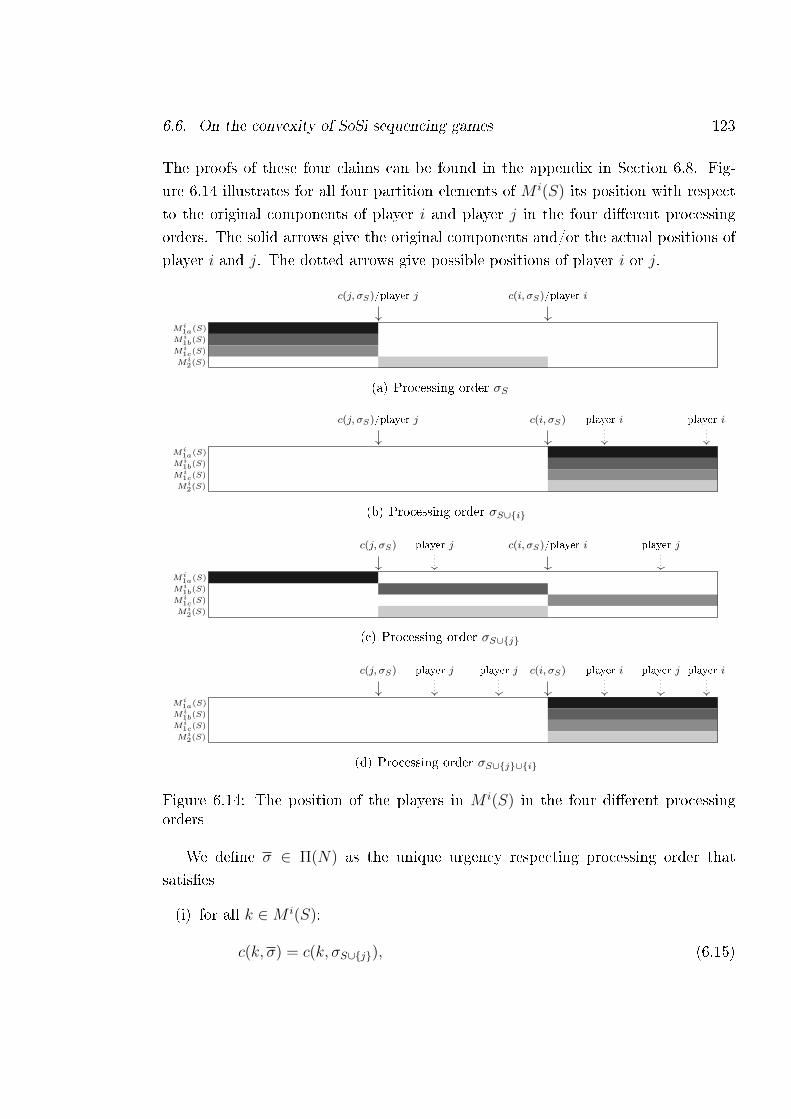
6.6. On the convexity of SoSi sequencing games 123
The proofs of these four claims can be found in the appendix in Section 6.8. Fig-
ure 6.14 illustrates for all four partition elements of M i(S) its position with respect
to the original components of player i and player j in the four dierent processing
orders. The solid arrows give the original components and/or the actual positions of
player i and j. The dotted arrows give possible positions of player i or j.
c(j, σS)/player j c(i, σS)/player i
Mi1a(S)
Mi1b(S)
Mi1c(S)
Mi2(S)
(a) Processing order σS
c(j, σS)/player j c(i, σS) player i player i
Mi1a(S)
Mi1b(S)
Mi1c(S)
Mi2(S)
(b) Processing order σS∪i
c(j, σS) player j c(i, σS)/player i player j
Mi1a(S)
Mi1b(S)
Mi1c(S)
Mi2(S)
(c) Processing order σS∪j
c(j, σS) c(i, σS) player i player jplayer j player j player i
Mi1a(S)
Mi1b(S)
Mi1c(S)
Mi2(S)
(d) Processing order σS∪j∪i
Figure 6.14: The position of the players in M i(S) in the four dierent processingorders
We dene σ ∈ Π(N) as the unique urgency respecting processing order that
satises
(i) for all k ∈M i(S):
c(k, σ) = c(k, σS∪j), (6.15)
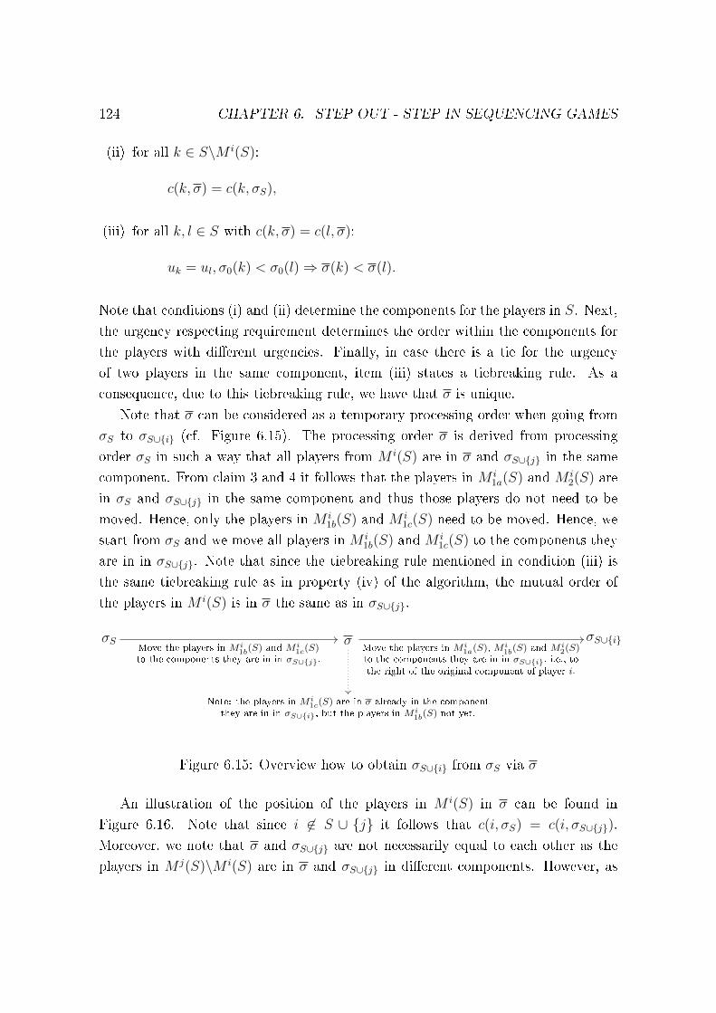
124 CHAPTER 6. STEP OUT - STEP IN SEQUENCING GAMES
(ii) for all k ∈ S\M i(S):
c(k, σ) = c(k, σS),
(iii) for all k, l ∈ S with c(k, σ) = c(l, σ):
uk = ul, σ0(k) < σ0(l)⇒ σ(k) < σ(l).
Note that conditions (i) and (ii) determine the components for the players in S. Next,
the urgency respecting requirement determines the order within the components for
the players with dierent urgencies. Finally, in case there is a tie for the urgency
of two players in the same component, item (iii) states a tiebreaking rule. As a
consequence, due to this tiebreaking rule, we have that σ is unique.
Note that σ can be considered as a temporary processing order when going from
σS to σS∪i (cf. Figure 6.15). The processing order σ is derived from processing
order σS in such a way that all players from M i(S) are in σ and σS∪j in the same
component. From claim 3 and 4 it follows that the players in M i1a(S) and M i
2(S) are
in σS and σS∪j in the same component and thus those players do not need to be
moved. Hence, only the players in M i1b(S) and M i
1c(S) need to be moved. Hence, we
start from σS and we move all players in M i1b(S) and M i
1c(S) to the components they
are in in σS∪j. Note that since the tiebreaking rule mentioned in condition (iii) is
the same tiebreaking rule as in property (iv) of the algorithm, the mutual order of
the players in M i(S) is in σ the same as in σS∪j.
σS σ σS∪i
Note: the players in M i1c(S) are in σ already in the component
they are in in σS∪i, but the players in M i1b(S) not yet.
Move the players in M i1b(S) and M i
1c(S)to the components they are in in σS∪j.
Move the players in M i1a(S), M i
1b(S) and M i2(S)
to the components they are in in σS∪i, i.e., tothe right of the original component of player i.
Figure 6.15: Overview how to obtain σS∪i from σS via σ
An illustration of the position of the players in M i(S) in σ can be found in
Figure 6.16. Note that since i 6∈ S ∪ j it follows that c(i, σS) = c(i, σS∪j).
Moreover, we note that σ and σS∪j are not necessarily equal to each other as the
players in M j(S)\M i(S) are in σ and σS∪j in dierent components. However, as
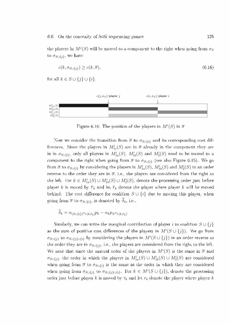
6.6. On the convexity of SoSi sequencing games 125
the players in M j(S) will be moved to a component to the right when going from σS
to σS∪j, we have
c(k, σS∪j) ≥ c(k, σ), (6.16)
for all k ∈ S ∪ j ∪ i.
c(j, σS)/player j c(i, σS)/player i
Mi1a(S)
Mi1b(S)
Mi1c(S)
Mi2(S)
Figure 6.16: The position of the players in M i(S) in σ
Now we consider the transition from σ to σS∪i and its corresponding cost dif-
ferences. Since the players in M i1c(S) are in σ already in the component they are
in in σS∪i, only all players in M i1a(S), M i
1b(S) and M i2(S) need to be moved to a
component to the right when going from σ to σS∪i (see also Figure 6.15). We go
from σ to σS∪i by considering the players inM i1a(S), M i
1b(S) andM i2(S) in an order
reverse to the order they are in σ, i.e., the players are considered from the right to
the left. For k ∈ M i1a(S) ∪M i
1b(S) ∪M i2(S), denote the processing order just before
player k is moved by τ k and let rk denote the player where player k will be moved
behind. The cost dierence for coalition S ∪ i due to moving this player, when
going from σ to σS∪i, is denoted by δk, i.e.,
δk = α(S∪i)τk (k,rk]pk − αkpNτk (k,rk].
Similarly, we can write the marginal contribution of player i to coalition S ∪ jas the sum of positive cost dierences of the players in M i(S ∪ j). We go from
σS∪j to σS∪j∪i by considering the players in M i(S ∪ j) in an order reverse to
the order they are in σS∪j, i.e., the players are considered from the right to the left.
We note that since the mutual order of the players in M i(S) is the same in σ and
σS∪j, the order in which the players in M i1a(S) ∪M i
1b(S) ∪M i2(S) are considered
when going from σ to σS∪i is the same as the order in which they are considered
when going from σS∪j to σS∪j∪i. For k ∈ M i(S ∪ j), denote the processing
order just before player k is moved by τk and let rk denote the player where player k
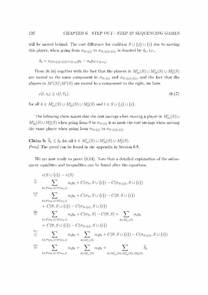
126 CHAPTER 6. STEP OUT - STEP IN SEQUENCING GAMES
will be moved behind. The cost dierence for coalition S ∪ j ∪ i due to moving
this player, when going from σS∪j to σS∪j∪i, is denoted by δk, i.e.,
δk = α(S∪j∪i)τk (k,rk]pk − αkpNτk (k,rk].
From (6.16) together with the fact that the players in M i1a(S) ∪M i
1b(S) ∪M i2(S)
are moved to the same component in σS∪i and σS∪j∪i, and the fact that the
players in M j(S)\M i(S) are moved to a component to the right, we have
c(l, τk) ≥ c(l, τ k), (6.17)
for all k ∈M i1a(S) ∪M i
1b(S) ∪M i2(S) and l ∈ S ∪ j ∪ i.
The following claim states that the cost savings when moving a player inM i1a(S)∪
M i1b(S)∪M i
2(S) when going from σ to σS∪i is at most the cost savings when moving
the same player when going from σS∪j to σS∪j∪i.
Claim 5: δk ≤ δk for all k ∈M i1a(S) ∪M i
1b(S) ∪M i2(S).
Proof. The proof can be found in the appendix in Section 6.8.
We are now ready to prove (6.14). Note that a detailed explanation of the subse-
quent equalities and inequalities can be found after the equations.
v(S ∪ i)− v(S)(i)=
∑k∈P (σ0,i)∩F (σS ,i)
αipk + C(σS, S ∪ i)− C(σS∪i, S ∪ i)
(ii)=
∑k∈P (σ0,i)∩F (σS ,i)
αipk + C(σS, S ∪ i)− C(σ, S ∪ i)
+ C(σ, S ∪ i)− C(σS∪i, S ∪ i)(iii)=
∑k∈P (σ0,i)∩F (σS ,i)
αipk + C(σS, S)− C(σ, S) +∑
k∈M i1c(S)
αipk
+ C(σ, S ∪ i)− C(σS∪i, S ∪ i)(iv)
≤∑
k∈P (σ0,i)∩F (σS ,i)
αipk +∑
k∈M i1c(S)
αipk + C(σ, S ∪ i)− C(σS∪i, S ∪ i)
(v)=
∑k∈P (σ0,i)∩F (σS ,i)
αipk +∑
k∈M i1c(S)
αipk +∑
k∈M i1a(S)∪M i
1b(S)∪M i2(S)
δk
6.6. On the convexity of SoSi sequencing games 127
(vi)
≤∑
k∈P (σ0,i)∩F (σS ,i)
αipk +∑
k∈M i1c(S)
αipk +∑
k∈M i1a(S)∪M i
1b(S)∪M i2(S)
δk
(vii)
≤∑
k∈P (σ0,i)∩F (σS ,i)
αipk +∑
k∈M i1c(S)
αipk +∑
k∈M i(S∪j)
δk
(viii)=
∑k∈P (σ0,i)∩F (σS ,i)
αipk +∑
k∈M i1c(S)
αipk
+ C(σS∪j, S ∪ j ∪ i)− C(σS∪j∪i, S ∪ j ∪ i)(ix)
≤∑
k∈P (σ0,i)∩F (σS ,i)
αipk +∑
k∈P (σS ,i)∩F (σS∪j,i)
αipk
+ C(σS∪j, S ∪ j ∪ i)− C(σS∪j∪i, S ∪ j ∪ i)(x)=
∑k∈P (σ0,i)∩F (σS∪j,i)
αipk + C(σS∪j, S ∪ j ∪ i)− C(σS∪j∪i, S ∪ j ∪ i)
(xi)= v(S ∪ j ∪ i)− v(S ∪ j),
which proves (6.14).
Explanations:
(i) The extra worth that is obtained by adding player i to coalition S can be split
into two parts. The rst part is due to the fact that player i joins the coalition
and it represents the cost savings for player i in processing order σS compared
to σ0. The completion time of player i is reduced by the sum of the processing
times of the players that jumped over player i when going from σ0 to σS without
moving any players. The second part represents the cost savings for coalition
S ∪ i by additionally moving players when going from σS to the optimal
processing order σS∪i.
(ii) The optimal processing order σS∪i can be obtained from σS via σ where some
players are already (partially) moved to the right.
(iii) The cost dierence for coalition S ∪ i when going from σS to σ can be split
into two parts: the cost dierence for coalition S and the cost dierence for
player i. By the denition of σ and since i 6∈ S ∪ j, player i is not moved
when going from σS to σ and the completion time of player i is reduced by the
sum of the processing times of the players that jumped over player i when going
from σS to σ, i.e., the sum of the processing times of the players in M i1c(S).
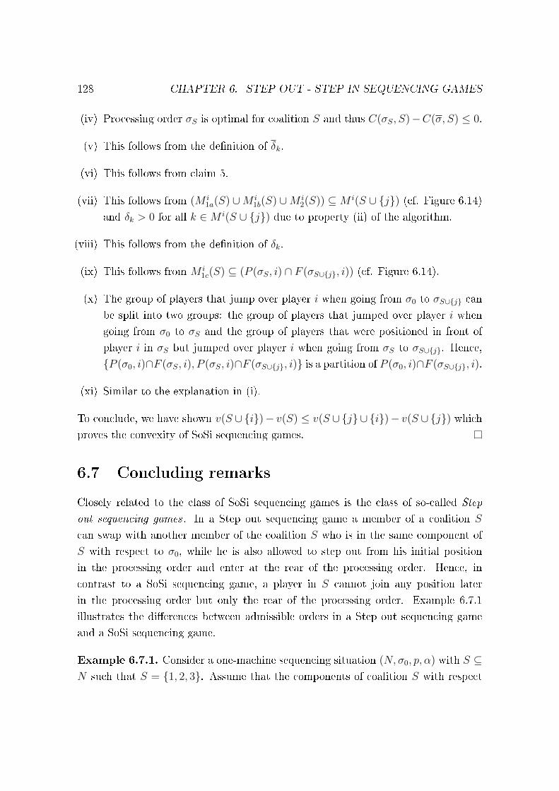
128 CHAPTER 6. STEP OUT - STEP IN SEQUENCING GAMES
(iv) Processing order σS is optimal for coalition S and thus C(σS, S)−C(σ, S) ≤ 0.
(v) This follows from the denition of δk.
(vi) This follows from claim 5.
(vii) This follows from (M i1a(S) ∪M i
1b(S) ∪M i2(S)) ⊆M i(S ∪ j) (cf. Figure 6.14)
and δk > 0 for all k ∈M i(S ∪ j) due to property (ii) of the algorithm.
(viii) This follows from the denition of δk.
(ix) This follows from M i1c(S) ⊆ (P (σS, i) ∩ F (σS∪j, i)) (cf. Figure 6.14).
(x) The group of players that jump over player i when going from σ0 to σS∪j can
be split into two groups: the group of players that jumped over player i when
going from σ0 to σS and the group of players that were positioned in front of
player i in σS but jumped over player i when going from σS to σS∪j. Hence,
P (σ0, i)∩F (σS, i), P (σS, i)∩F (σS∪j, i) is a partition of P (σ0, i)∩F (σS∪j, i).
(xi) Similar to the explanation in (i).
To conclude, we have shown v(S ∪i)− v(S) ≤ v(S ∪j∪ i)− v(S ∪j) whichproves the convexity of SoSi sequencing games.
6.7 Concluding remarks
Closely related to the class of SoSi sequencing games is the class of so-called Step
out sequencing games . In a Step out sequencing game a member of a coalition S
can swap with another member of the coalition S who is in the same component of
S with respect to σ0, while he is also allowed to step out from his initial position
in the processing order and enter at the rear of the processing order. Hence, in
contrast to a SoSi sequencing game, a player in S cannot join any position later
in the processing order but only the rear of the processing order. Example 6.7.1
illustrates the dierences between admissible orders in a Step out sequencing game
and a SoSi sequencing game.
Example 6.7.1. Consider a one-machine sequencing situation (N, σ0, p, α) with S ⊆N such that S = 1, 2, 3. Assume that the components of coalition S with respect
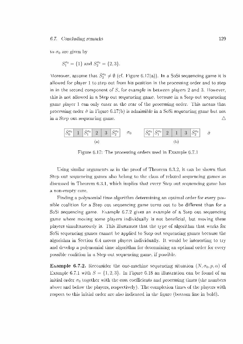
6.7. Concluding remarks 129
to σ0 are given by
Sσ01 = 1 and Sσ02 = 2, 3.
Moreover, assume that Sσ02 6= ∅ (cf. Figure 6.17(a)). In a SoSi sequencing game it is
allowed for player 1 to step out from his position in the processing order and to step
in in the second component of S, for example in between players 2 and 3. However,
this is not allowed in a Step out sequencing game, because in a Step out sequencing
game player 1 can only enter at the rear of the processing order. This means that
processing order σ in Figure 6.17(b) is admissible in a SoSi sequencing game but not
in a Step out sequencing game. 4
Sσ00 1 Sσ01 2 3 Sσ02σ0
(a)
Sσ00 Sσ01 2 1 3 Sσ02 σ
(b)
Figure 6.17: The processing orders used in Example 6.7.1
Using similar arguments as in the proof of Theorem 6.3.2, it can be shown that
Step out sequencing games also belong to the class of relaxed sequencing games as
discussed in Theorem 6.3.1, which implies that every Step out sequencing game has
a non-empty core.
Finding a polynomial time algorithm determining an optimal order for every pos-
sible coalition for a Step out sequencing game turns out to be dierent than for a
SoSi sequencing game. Example 6.7.2 gives an example of a Step out sequencing
game where moving some players individually is not benecial, but moving these
players simultaneously is. This illustrates that the type of algorithm that works for
SoSi sequencing games cannot be applied to Step out sequencing games because the
algorithm in Section 6.4 moves players individually. It would be interesting to try
and develop a polynomial time algorithm for determining an optimal order for every
possible coalition in a Step out sequencing game, if possible.
Example 6.7.2. Reconsider the one-machine sequencing situation (N, σ0, p, α) of
Example 6.7.1 with S = 1, 2, 3. In Figure 6.18 an illustration can be found of an
initial order σ0 together with the cost coecients and processing times (the numbers
above and below the players, respectively). The completion times of the players with
respect to this initial order are also indicated in the gure (bottom line in bold).
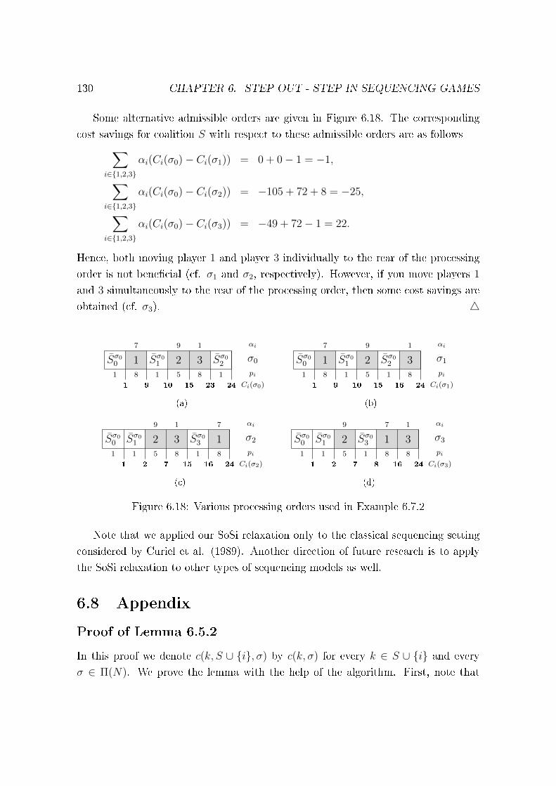
130 CHAPTER 6. STEP OUT - STEP IN SEQUENCING GAMES
Some alternative admissible orders are given in Figure 6.18. The corresponding
cost savings for coalition S with respect to these admissible orders are as follows∑i∈1,2,3
αi(Ci(σ0)− Ci(σ1)) = 0 + 0− 1 = −1,
∑i∈1,2,3
αi(Ci(σ0)− Ci(σ2)) = −105 + 72 + 8 = −25,
∑i∈1,2,3
αi(Ci(σ0)− Ci(σ3)) = −49 + 72− 1 = 22.
Hence, both moving player 1 and player 3 individually to the rear of the processing
order is not benecial (cf. σ1 and σ2, respectively). However, if you move players 1
and 3 simultaneously to the rear of the processing order, then some cost savings are
obtained (cf. σ3). 4
Sσ00
1
1
1
7
8
9
Sσ01
1
10
2
9
5
15
3
1
8
23
Sσ02
1
24
αi
σ0
pi
Ci(σ0)
(a)
Sσ00
1
1
1
7
8
9
Sσ01
1
10
2
9
5
15
Sσ02
1
16
3
1
8
24
αi
σ1
pi
Ci(σ1)
(b)
Sσ00
1
1
Sσ01
1
2
2
9
5
7
3
1
8
15
Sσ03
1
16
1
7
8
24
αi
σ2
pi
Ci(σ2)
(c)
Sσ00
1
1
Sσ01
1
2
2
9
5
7
Sσ03
1
8
1
7
8
16
3
1
8
24
αi
σ3
pi
Ci(σ3)
(d)
Figure 6.18: Various processing orders used in Example 6.7.2
Note that we applied our SoSi relaxation only to the classical sequencing setting
considered by Curiel et al. (1989). Another direction of future research is to apply
the SoSi relaxation to other types of sequencing models as well.
6.8 Appendix
Proof of Lemma 6.5.2
In this proof we denote c(k, S ∪ i, σ) by c(k, σ) for every k ∈ S ∪ i and every
σ ∈ Π(N). We prove the lemma with the help of the algorithm. First, note that
6.8. Appendix 131
because player i is the only player in its component in σ0, we have σS0 = σS∪i0 ,
i.e., the processing orders are the same after the preprocessing step of the algorithm.
Therefore, if we go from σ0 to the optimal processing orders σS and σS∪i, then the
steps performed by the algorithm are the same up to the moment that player i is
considered. Moreover, since the players are considered in reverse order with respect
to σS0 , we have
c(k, σS∪i) = c(k, σS), (6.18)
for all k ∈ S ∩ F (σS0 , i). Hence, it remains to be proven that also for the players in
S ∩ P (σS0 , i) the lemma is true.
Let player m ∈ S be the closest predecessor of player i with respect to σS0 for
which the lemma is not true, i.e.,
c(m,σS∪i) < c(m,σS),
and
c(k, σS∪i) ≥ c(k, σS),
for all k ∈ S ∩ F (σS0 ,m) ∩ P (σS0 , i). We will derive a contradiction. We continue
the proof as follows. We look to which component player m will be moved by the
algorithm with respect to coalition S. Then, there is a specic player who is in a
component with index at least as high as the component that player m is moved by
the algorithm with respect to coalition S. We show that moving player m behind
this specic player is actually more benecial with respect to coalition S ∪i, whichcontradicts the optimality of the algorithm.
Denote the processing order when player m is considered by the algorithm with
respect to coalition S by τS and with respect to coalition S ∪ i by τS∪i. Let rS
denote the player where player m will be moved behind with respect to coalition S
according to the algorithm. Similarly, let rS∪i denote the player where player m
will be moved behind with respect to coalition S ∪ i according to the algorithm.
Note that in case player m is not moved by the algorithm with respect to coalition
S∪i, then we dene player rS∪i as player m. Since c(m,σS∪i) = c(rS∪i, τS∪i)
and c(m,σS) = c(rS, τS), we have
c(rS∪i, τS∪i) < c(rS, τS). (6.19)
132 CHAPTER 6. STEP OUT - STEP IN SEQUENCING GAMES
As we will see later (S ∪ i)σ0,τS
c(rS∪i,τS∪i)6= ∅, let rS ∈ (S ∪ i)σ0,τ
S
c(rS∪i,τS∪i)be
such that player m would be moved behind this player in case player m is moved to
component (S∪i)σ0,τS
c(rS∪i,τS∪i)according to the algorithm with respect to coalition
S . Note that player rS is unique because the algorithm always selects a unique player
per component. Note that player rS might also be player i as in this way we make
sure that player rS also exists if c(rS∪i, τS∪i) = c(i, σ0).6 Note that in case player
m and rS∪i coincide (that means that player m is not moved by the algorithm with
respect to coalition S ∪ i), then we dene player rS as player m.
Since player m is moved behind player rS and not behind player rS, we have due
to property (v) of the algorithm that
αSτS (rS ,rS ]pm − αmpNτS (rS ,rS ] > 0. (6.20)
We distinguish between two cases:
case A: k ∈ S | σS0 (m) < σS0 (k) < σS0 (i) = ∅,
case B: k ∈ S | σS0 (m) < σS0 (k) < σS0 (i) 6= ∅.
Case A: [k ∈ S | σS0 (m) < σS0 (k) < σS0 (i) 6= ∅]Hence, there are no players of coalition S in between player m and player i in σS0 .
Then, from (6.18) it follows that for every k ∈ S ∩ F (τS,m) we have
c(k, τS) = c(k, τS∪i). (6.21)
Note that this implies that (S ∪ i)σ0,τS
c(rS∪i,τS∪i)is non-empty.
We will prove that moving player m behind player rS is more benecial than
moving player m behind player rS∪i, i.e., we will prove that
α(S∪i)τS∪i (rS∪i,rS ]
pm − αmpNτS∪i (rS∪i,rS ]> 0. (6.22)
This would imply that the step made by the algorithm for player m when applied on
coalition S ∪ i is not optimal, which contradicts the optimality of the algorithm.
Hence, for case A, it remains to prove (6.22).
We distinguish from now on between the following four cases:
6Note that in case c(rS∪i, τS∪i) = c(i, σ0) it is not admissible for the algorithm to move
player m to component (S ∪ i)σ0,τS
c(rS∪i,τS∪i)due to requirement (ii) of admissibility, but this is
no problem as also in this case the upcoming arguments are still valid.
6.8. Appendix 133
case A.1: i 6∈ N τS(rS, rS] and i 6∈ N τS∪i(rS∪i, rS],
case A.2: i ∈ N τS(rS, rS] and i 6∈ N τS∪i(rS∪i, rS],
case A.3: i ∈ N τS(rS, rS] and i ∈ N τS∪i(rS∪i, rS],
case A.4: i 6∈ N τS(rS, rS] and i ∈ N τS∪i(rS∪i, rS].
Case A.1: [i 6∈ N τS(rS, rS] and i 6∈ N τS∪i(rS∪i, rS]]
Note that this case occurs if rS∪i 6= m and player i is not necessarily moved by the
algorithm with respect to coalition S∪i. Then, it follows from (6.21) together with
the fact c(rS, τS) = c(rS∪i, τS∪i) that
α(S∪i)τS∪i (rS∪i,rS ]
pm − αmpNτS∪i (rS∪i,rS ]
= αSτS (rS ,rS ]pm − αmpNτS (rS ,rS ]
(6.20)> 0.
Case A.2: [i ∈ N τS(rS, rS] and i 6∈ N τS∪i(rS∪i, rS]]
Note that this case occurs if rS∪i = m and player i has been moved by the algorithm
with respect to coalition S ∪ i such that τS∪i(i) > τS∪i(rS). Then, using the
same arguments as in case A.1, we have
α(S∪i)τS∪i (rS∪i,rS ]
pm − αmpNτS∪i (rS∪i,rS ]
= αSτS (rS ,rS ]pm − αmpNτS (rS ,rS ] + αmpi(6.20)> 0.
Case A.3: [i ∈ N τS(rS, rS] and i ∈ N τS∪i(rS∪i, rS]]
Note that this case occurs if rS∪i = m and player i has either not been moved
by the algorithm with respect to coalition S ∪ i or it has been moved such that
τS∪i(i) < τS∪i(rS). Then, using the same arguments as in case A.1, we have
α(S∪i)τS∪i (rS∪i,rS ]
pm − αmpNτS∪i (rS∪i,rS ]
= αSτS (rS ,rS ]pm − αmpNτS (rS ,rS ] + αipm(6.20)> 0.
Case A.4: [i 6∈ N τS(rS, rS] and i ∈ N τS∪i(rS∪i, rS]]
Note that this case occurs if rS∪i 6= m and player i has been moved by the algorithm
134 CHAPTER 6. STEP OUT - STEP IN SEQUENCING GAMES
with respect to coalition S ∪ i such that τS∪i(rS∪i) < τS∪i(i) < τS∪i(rS).
Then, using the same arguments as in case A.1, we have
α(S∪i)τS∪i (rS∪i,rS ]
pm − αmpNτS∪i (rS∪i,rS ]
= αSτS (rS ,rS ]pm − αmpNτS (rS ,rS ] + αipm − αmpi.
If we can show that αipm − αmpi > 0, (6.22) follows.
Let rS be the direct predecessor of player i in τS∪i. Since player i is moved
behind player rS and not behind player rS, we have due to the optimality of the
algorithm that
α(S∪i)τS∪i (i,rS ]
pi − αipNτS∪i (i,rS ]≤ 0.
Consequently, it follows from (6.21) together with the fact c(rS, τS) = c(i, τS∪i)
that we also have
αSτS (rS ,rS ]pi − αipNτS (rS ,rS ] ≤ 0.
Therefore, together with (6.20), we can conclude αipi> αm
pm, i.e., αipm − αmpi > 0.
Case B: [k ∈ S | σS0 (m) < σS0 (k) < σS0 (i) 6= ∅]Hence, there are players of coalition S in between player m and player i in σS0 .
Therefore, due to the denition of player m, it follows that for every k ∈ S with
σS0 (m) < σS0 (k) < σS0 (i) we have
c(k, σS∪i) ≥ c(k, σS), (6.23)
i.e., the statement in the lemma holds for all followers of player m with respect to
σS0 intersected with S ∩P (σS0 , i). First, note that (S ∪i)σ0,τS
c(rS∪i,τS∪i)is non-empty
because of the following. Due to requirement (i) and (ii) of admissibility we know
that the rst player in (S ∪ i)σ0,τS∪i
c(rS∪i,τS∪i)with respect to τS∪i is also the rst
player in (S ∪ i)σ0,σS0
c(rS∪i,τS∪i)with respect to σS0 . Therefore, using (6.23) we know
that this player also belongs to (S ∪ i)σ0,τS
c(rS∪i,τS∪i). Hence, (S ∪ i)σ0,τ
S
c(rS∪i,τS∪i)
is non-empty.
Next, dene player l ∈ SτS(rS, rS] as the player in SτS(rS, rS] who is positioned
last with respect to τS∪i, i.e., τS∪i(l) ≥ τS∪i(k) for all k ∈ SτS(rS, rS]. Note that
player l was actually player rS in case A because of (6.21). From the assumptions
in (6.23) and (6.19) it follows that
c(l, τS∪i) ≥ c(rS, τS∪i) ≥ c(rS, τS) > c(rS∪i, τS∪i), (6.24)
6.8. Appendix 135
i.e., player l is to the right of player rS∪i in τS∪i. We will prove that moving player
m behind player l is more benecial than moving player m behind player rS∪i, i.e.,
we will prove that
α(S∪i)τS∪i (rS∪i,l]
pm − αmpNτS∪i (rS∪i,l]> 0. (6.25)
This implies that the step made by the algorithm for player m when applied on
coalition S ∪ i is not optimal, which contradicts the optimality of the algorithm.
Hence, for case B, it remains to prove (6.25).
From the denitions of players rS and l, together with (6.23), it follows that
SτS
(rS, rS] ⊆ SτS∪i
(rS∪i, l] ⊆ (S ∪ i)τS∪i(rS∪i, l]. (6.26)
Moreover, since during the run of the algorithm player m jumps over all players in
SτS(m, rS], Lemma 6.4.1 implies that
uk > um, (6.27)
for all k ∈ SτS(m, rS].
Below we distinguish between the following four cases:
case B.1: i 6∈ N τS(rS, rS] and i 6∈ N τS∪i(rS∪i, l],
case B.2: i ∈ N τS(rS, rS] and i 6∈ N τS∪i(rS∪i, l],
case B.3: i ∈ N τS(rS, rS] and i ∈ N τS∪i(rS∪i, l],
case B.4: i 6∈ N τS(rS, rS] and i ∈ N τS∪i(rS∪i, l].
Case B.1: [i 6∈ N τS(rS, rS] and i 6∈ N τS∪i(rS∪i, l]]
Using c(l, τS∪i) ≥ c(rS, τS) from (6.24), we distinguish between another two cases:
case B.1(i): c(l, τS∪i) = c(rS, τS),
case B.1(ii): c(l, τS∪i) > c(rS, τS).
Case B.1(i): [c(l, τS∪i) = c(rS, τS)]
136 CHAPTER 6. STEP OUT - STEP IN SEQUENCING GAMES
Since rS ∈ (S ∪ i)σ0,τS
c(rS∪i,τS∪i)and thus c(rS, τS) = c(rS∪i, τS∪i), the assump-
tions i 6∈ N τS(rS, rS] and c(l, τS∪i) = c(rS, τS) imply that
SτS
(rS, rS] = SτS∪i
(rS∪i, l] = (S ∪ i)τS∪i(rS∪i, l]. (6.28)
For every k ∈ SτS∪i
(rS∪i, l]\SτS(rS, rS] we know that k ∈ SτS(m, rS], because
c(k, τS) ≤ c(k, τS∪i) by (6.23) and P (τS,m) = P (τS∪i,m). Hence, also k ∈Sτ
S(m, rS] and thus from (6.27) it follows that uk > um. Together with Proposi-
tion 6.5.1 applied on the set SτS∪i
(rS∪i, l]\SτS(rS, rS] and player m we have
α(S∪i)τS∪i (rS∪i,l]\SτS (rS ,rS ]
pm − αmp(S∪i)τS∪i (rS∪i,l]\SτS (rS ,rS ]
= αSτS∪i
(rS∪i,l]\SτS (rS ,rS ]pm − αmpSτS∪i (rS∪i,l]\SτS (rS ,rS ]
> 0, (6.29)
where the equality follows from the assumption i 6∈ N τS∪i(rS∪i, l]. As a conse-
quence,
α(S∪i)τS∪i (rS∪i,l]
pm − αmpNτS∪i (rS∪i,l]
= α(S∪i)τS∪i (rS∪i,l]
pm − αm(p
(S∪i)τS∪i (rS∪i,l]+ p
(S∪i)τS∪i (rS∪i,l]
)(6.28)= α
(S∪i)τS∪i (rS∪i,l]pm − αm
(p
(S∪i)τS∪i (rS∪i,l]+ p
SτS
(rS ,rS ]
)(6.26)= αSτS (rS ,rS ]pm − αm
(pSτS (rS ,rS ] + p
SτS
(rS ,rS ]
)+ α
(S∪i)τS∪i (rS∪i,l]\SτS (rS ,rS ]pm − αmp(S∪i)τS∪i (rS∪i,l]\SτS (rS ,rS ]
(6.29)
≥ αSτS (rS ,rS ]pm − αm(pSτS (rS ,rS ] + p
SτS
(rS ,rS ]
)(6.20)> 0,
proving (6.25).
Case B.1(ii): [c(l, τS∪i) > c(rS, τS)]
Dene Q as the set of players from SτS(rS, rS] who are positioned in τS∪i in a
component to the right of component (S ∪ i)σ0,τS∪i
c(rS ,τS). Since c(l, τS∪i) > c(rS, τS)
and l ∈ SτS(rS, rS], we have l ∈ Q and thus Q 6= ∅. Select from Q only the players
who have in their corresponding component in τS∪i no players from SτS(rS, rS] in
front of him and denote this set of players by Q, i.e., we select in each component a
player of Q (if possible) that is most to the left in τS∪i.
Set Q = q1, q2, . . . , q|Q| such that c(qk, τS∪i) < c(qk+1, τ
S∪i) for all k ∈1, . . . , |Q| − 1. Dene w1 as the rst player in (S ∪ i)
σ0
c(rS ,τS), i.e., the direct
6.8. Appendix 137
follower in τS∪i of component (S ∪ i)σ0,τS∪i
c(rS ,τS). For k ∈ 2, . . . , |Q|, dene wk as
the rst player in (S ∪ i)σ0
c(qk−1,τS∪i), i.e., the direct follower in τS∪i of compo-
nent (S ∪ i)σ0,τS∪i
c(qk−1,τS∪i). Note that because of the denition of player l we have
c(q|Q|, τS∪i) = c(l, τS∪i).
The collection of sets N τS∪i [wk, qk) | k ∈ 1, . . . , |Q| are by denition mutu-
ally disjoint. Moreover, for k ∈ 1, . . . , |Q|, we have N τS∪i [wk, qk)∩SτS(rS, rS] = ∅
and (S ∪ i)τS∪i [wk, qk) ⊆ (S ∪ i)τS∪i(rS∪i, l]. If we set R = SτS(rS, rS] ∪⋃|Q|
k=1 (S ∪ i)τS∪i [wk, qk), then using (6.26) we have
R ⊆ (S ∪ i)τS∪i(rS∪i, l], (6.30)
and
αR = αSτS (rS ,rS ] +
|Q|∑k=1
α(S∪i)τS∪i [wk,qk)
, (6.31)
and
pR = pSτS (rS ,rS ] +
|Q|∑k=1
p(S∪i)τS∪i [wk,qk)
. (6.32)
Note, for k ∈ 1, . . . , |Q|, we have c(qk, σ0) ≤ c(qk, τS) ≤ c(rS, τS). Hence,
as wk is in τS∪i to the right of component (S ∪ i)σ0,τS∪i
c(rS ,τS), we have that it is
admissible to more player qk in front of wk with respect to τS∪i. In other words,
it is admissible to move player qk to the tail of component (S ∪ i)σ0,τS∪i
c(qk−1,τS∪i)(and
the tail of component (S ∪ i)σ0,τS∪i
c(rS ,τS)in case k = 1). Since player qk is not moved
behind player wk, we have due to property (v) of the algorithm that
α(S∪i)τS∪i [wk,qk)
pqk − αqkpNτS∪i [wk,qk)> 0.
Moreover, since qk ∈ SτS(m, rS] it follows from (6.27) that um < uqk . As a conse-
quence,
α(S∪i)τS∪i [wk,qk)
pm − αmpNτS∪i [wk,qk)> 0. (6.33)
138 CHAPTER 6. STEP OUT - STEP IN SEQUENCING GAMES
We have
αRpm − αm(pR + p
(S∪i)τS∪i (rS∪i,l]
)(6.31),(6.32)
=
αSτS (rS ,rS ] +
|Q|∑k=1
α(S∪i)τS∪i [wk,qk)
pm
− αm
(pSτS (rS ,rS ] +
|Q|∑k=1
p(S∪i)τS∪i [wk,qk)
+p(S∪i)τS∪i (rS∪i,w1)
+ p(S∪i)τS∪i [w1,l]
)
see below=
αSτS (rS ,rS ] +
|Q|∑k=1
α(S∪i)τS∪i [wk,qk)
pm
− αm
(pSτS (rS ,rS ] +
|Q|∑k=1
p(S∪i)τS∪i [wk,qk)
+ pSτS
(rS ,rS ]+
|Q|∑k=1
p(S∪i)τS∪i [wk,qk)
)
=
αSτS (rS ,rS ] +
|Q|∑k=1
α(S∪i)τS∪i [wk,qk)
pm
−αm
pNτS (rS ,rS ] +
|Q|∑k=1
pNτS∪i [wk,qk)
(6.20),(6.33)
> 0. (6.34)
Note that the second equality follows from c(rS, τS) = c(rS∪i, τS∪i), the fact that
w1 is the direct follower in τS∪i of component (S ∪ i)σ0,τS∪i
c(rS ,τS), and the assump-
tion i 6∈ N τS(rS, rS]. Moreover, the collection of sets (S ∪ i)τS∪i [wk, qk) | k ∈1, . . . , |Q| forms a partition of the set (S ∪ i)τS∪i [w1, l].
For every k ∈ SτS∪i(rS∪i, l]\R, we know that either k ∈ SτS(m, rS] or c(k, τS) ≥c(rS, τS). If k ∈ SτS(m, rS], then also k ∈ SτS(m, rS] and thus from (6.27) we have
uk > um. Next, if c(k, τS) ≥ c(rS, τS), then because c(l, τS) ≤ c(rS, τS) we know
that the swap of players k and l with respect to τS∪i is admissible. Therefore,
according to Lemma 6.4.1, we know uk ≥ ul. Moreover, since l ∈ SτS(m, rS], it
follows from (6.27) that um < ul. As a consequence, um < uk. Together with
6.8. Appendix 139
Proposition 6.5.1 applied on the set SτS∪i
(rS∪i, l]\R and player m we have
α(S∪i)τS∪i (rS∪i,l]\Rpm − αmp(S∪i)τS∪i (rS∪i,l]\R
= αSτS∪i
(rS∪i,l]\Rpm − αmpSτS∪i (rS∪i,l]\R > 0, (6.35)
where the equality follows from the assumption i 6∈ N τS∪i(rS∪i, l]. As a conse-
quence,
α(S∪i)τS∪i (rS∪i,l]
pm − αmpNτS∪i (rS∪i,l]
= α(S∪i)τS∪i (rS∪i,l]
pm − αm(p
(S∪i)τS∪i (rS∪i,l]+ p
(S∪i)τS∪i (rS∪i,l]
)(6.30)= αRpm − αm
(pR + p
(S∪i)τS∪i (rS∪i,l]
)+ α
(S∪i)τS∪i (rS∪i,l]\Rpm − αmp(S∪i)τS∪i (rS∪i,l]\R(6.34),(6.35)
> 0,
proving (6.25).
Case B.2: [i ∈ N τS(rS, rS] and i 6∈ N τS∪i(rS∪i, l]]
Note that this case occurs exactly if c(rS, τS) < c(i, σ0) < c(rS, τS) and player i has
been moved by the algorithm with respect to coalition S ∪ i such that τS∪i(i) >
τS∪i(l). We have
αSτS (rS ,rS ]pm−αmpNτS (rS ,rS ]\i = αSτS (rS ,rS ]pm−αmpNτS (rS ,rS ]+αmpi(6.20)> 0. (6.36)
Then, using the same arguments as in case B.1, we can prove (6.25). Namely, where
we used (6.20) in case B.1, we now use the above equation. Hence, player i has
already been taken into account and thus for using the same arguments as in case
B.1 we can assume i 6∈ N τS(rS, rS] and i 6∈ N τS∪i(rS∪i, l].
For example, analogous to case B.1(i), case B.2(i) goes as follows. Since rS ∈ (S∪i)σ0,τ
S
c(rS∪i,τS∪i)and thus c(rS, τS) = c(rS∪i, τS∪i), the assumption c(l, τS∪i) =
c(rS, τS) implies that
SτS
(rS, rS]\i = SτS∪i
(rS∪i, l] = (S ∪ i)τS∪i(rS∪i, l]. (6.37)
Using exactly the same arguments as in case B.1(i) we have
α(S∪i)τS∪i (rS∪i,l]\SτS (rS ,rS ]
pm − αmp(S∪i)τS∪i (rS∪i,l]\SτS (rS ,rS ]> 0, (6.38)
140 CHAPTER 6. STEP OUT - STEP IN SEQUENCING GAMES
As a consequence,
α(S∪i)τS∪i (rS∪i,l]
pm − αmpNτS∪i (rS∪i,l]
= α(S∪i)τS∪i (rS∪i,l]
pm − αm(p
(S∪i)τS∪i (rS∪i,l]+ p
(S∪i)τS∪i (rS∪i,l]
)(6.37)= α
(S∪i)τS∪i (rS∪i,l]pm − αm
(p
(S∪i)τS∪i (rS∪i,l]+ p
SτS
(rS ,rS ]\i
)(6.26)= αSτS (rS ,rS ]pm − αm
(pSτS (rS ,rS ] + p
SτS
(rS ,rS ]\i
)+ α
(S∪i)τS∪i (rS∪i,l]\SτS (rS ,rS ]pm − αmp(S∪i)τS∪i (rS∪i,l]\SτS (rS ,rS ]
(6.38)
≥ αSτS (rS ,rS ]pm − αm(pSτS (rS ,rS ] + p
SτS
(rS ,rS ]\i
)= αSτS (rS ,rS ]pm − αmpNτS (rS ,rS ]\i
(6.36)> 0,
proving (6.25).
Case B.3: [i ∈ N τS(rS, rS] and i ∈ N τS∪i(rS∪i, l]]
Note that this case occurs exactly if c(rS, τS) < c(i, σ0) < c(rS, τS) and player i has
either not been moved by the algorithm with respect to coalition S ∪ i or it hasbeen moved such that τS∪i(i) < τS∪i(l). We have
αSτS (rS ,rS ]∪ipm − αmpNτS (rS ,rS ] = αSτS (rS ,rS ]pm − αmpNτS (rS ,rS ] + αipm(6.20)> 0.
Then, using the same arguments as in case B.1, we can prove (6.25).
Case B.4: [i 6∈ N τS(rS, rS] and i ∈ N τS∪i(rS∪i, l]]
Then,
αSτS (rS ,rS ]∪ipm−αmpNτS (rS ,rS ]∪i = αSτS (rS ,rS ]pm−αmpNτS (rS ,rS ] +αipm−αmpi.
It suces to show that αipm−αmpi > 0. Together with the above equation and (6.20),
we can prove (6.25) by using the same arguments as in case B.1.
We distinguish between two cases:
case B.4(i): c(i, σ0) > c(rS, τS),
case B.4(ii): c(i, σ0) < c(rS, τS).
6.8. Appendix 141
Case B.4(i): [c(i, σ0) > c(rS, τS)]
Note that this case occurs exactly if τS∪i(i) < τS∪i(l). This means that player i
is not necessarily moved by the algorithm with respect to coalition S ∪ i. Then,
c(l, σ0) ≤ c(l, τS) ≤ c(rS, τS) < c(i, σ0) ≤ c(i, τS∪i) = c(i, σS∪i).
Hence, the swap of players i and l with respect to σS∪i is admissible and thus,
according to Lemma 6.4.1, we have ui ≥ ul. Consequently, together with (6.27), we
have ui ≥ ul > um. Hence, αipm − αmpi > 0.
Case B.4(ii): [c(i, σ0) < c(rS, τS)]
Note that this case occurs exactly if player i has been moved by the algorithm with
respect to coalition S ∪ i such that τS∪i(rS∪i) < τS∪i(i) < τS∪i(l). Suppose
c(l, σ0) < c(i, σ0), then
c(l, σ0) < c(i, σ0) < c(rS, τS) = c(rS∪i, τS∪i) = c(m,σS∪i).
Hence, the swap of players m and l with respect to σS∪i is admissible and thus,
according to Lemma 6.4.1, we have um ≥ ul. This is a contradiction with (6.27)
and thus we know c(l, σ0) > c(i, σ0). Therefore, using (6.18), we have c(l, τS) =
c(l, τS∪i) which implies l = rS. As a consequence, if k ∈ SτS∪i
(rS∪i, rS], then
also k ∈ SτS(m, rS] and thus from (6.27) we have um < uk. With the same arguments
we used for player l we can conclude c(k, σ0) > c(i, σ0) and thus c(k, τS) = c(k, τS∪i).
Therefore, we have
N τS(rS, rS] ∪ i = N τS∪i(rS∪i, rS], (6.39)
and
c(k, τS) = c(k, τS∪i), (6.40)
for all k ∈ SτS(rS, rS].
Let rS be the direct predecessor of player i in τS∪i. Since player i is in τS∪i
behind player rS and not behind player rS, although this is an admissible swap, we
have
α(S∪i)τS∪i (i,rS ]
pi − αipNτS∪i (i,rS ]≤ 0.
142 CHAPTER 6. STEP OUT - STEP IN SEQUENCING GAMES
Consequently, it follows from (6.39) and (6.40) together with the fact that c(rS, τS) =
c(i, τS∪i), that
αSτS (rS ,rS ]pi − αipNτS (rS ,rS ] ≤ 0.
Moreover, since player m is moved behind player rS and not behind player rS, we
have due to property (v) of the algorithm that
αSτS (rS ,rS ]pm − αmpNτS (rS ,rS ] > 0.
Therefore, we can conclude αipi> αm
pm, i.e., αipm−αmpi > 0, which is exactly what we
needed.
Proof of Lemma 6.5.6
In this proof we denote c(k, S ∪ i, σ) by c(k, σ) for every k ∈ S ∪ i and every
σ ∈ Π(N). We continue the proof by means of induction on the number
nm = j ∈ S | σS(m) < σS(j) < σS(i),
i.e., the number of players in coalition S between player m and player i in σS.
Base step: If nm = 0, then player m is among all players in S the closest predecessor
of player i with respect to σS. Then,
l ∈ S ∩ F (τm,m) | c(l, τm) < c(i, σ0) = ∅,
and thus (6.10) is true.
Induction step: Assume that (6.10) holds for every k ∈ S ∩ P (σS, i) with nk < nm.
Since the followers of player m with respect to σS intersected with S ∩ P (σS, i) are
exactly the players with nk < nm, we actually assume that for every k ∈ S∩P (σS, i)∩F (σS,m) and r ∈ S ∩ F (τk, k) with c(r, τk) < c(i, σ0) we have
α(S∪i)τk (k,r]pk − αkpNτk (k,r] ≤ 0, (6.41)
We distinguish between the following cases:
um ≤ uk for all k ∈ SσS(m, l],
6.8. Appendix 143
there exists a player k ∈ SσS(m, l] with um > uk.
Case 1: [um ≤ uk for all k ∈ SσS(m, l]]
We will show that since moving player m behind player l in σS is not benecial, also
moving player m behind player l in τm is not benecial.
Note that because of the induction assumption in (6.41), we know that all players
in (S ∪ i)τm(m, l] have not been moved by the algorithm and thus N τm(m, l] ⊆NσS(m, l]. Moreover, since player l is in both σS and τm to the left of the original
component of player i in σ0, we have
(S ∪ i)τm(m, l] ⊆ SσS(m, l], (6.42)
and
(S ∪ i)τm(m, l] = SσS
(m, l]. (6.43)
Note, as processing order σS is optimal for coalition S, we have
αSσS (m,l]pm − αmpNσS (m,l] ≤ 0. (6.44)
Since um ≤ uk for all k ∈ SσS(m, l], it follows from Proposition 6.5.1 applied on the
set SσS(m, l] and player m together with (6.42) that
αSσS (m,l]\(S∪i)τm (m,l]pm − αmpSσS (m,l]\(S∪i)τm (m,l] ≥ 0, (6.45)
where there is an equality if SσS(m, l] = (S∪i)τm(m, l]. As a consequence, we have
α(S∪i)τm (m,l]pm − αmpNτm (m,l]
= α(S∪i)τm (m,l]pm − αm(p(S∪i)τm (m,l] + p(S∪i)τm (m,l]
)(6.42),(6.43)
= αSσS (m,l]pm − αm(pSσS (m,l] + pSσS (m,l]
)−(αSσS (m,l]\(S∪i)τm (m,l]pm − αmpSσS (m,l]\(S∪i)τm (m,l]
)= αSσS (m,l]pm − αmpNσS (m,l]
−(αSσS (m,l]\(S∪i)τm (m,l]pm − αmpSσS (m,l]\(S∪i)τm (m,l]
)(6.44),(6.45)
≤ 0,
and (6.10) follows.
144 CHAPTER 6. STEP OUT - STEP IN SEQUENCING GAMES
Case 2: [there exists a player k ∈ SσS(m, l] with um > uk]
Let player q ∈ SσS(m, l] be the closest follower of player m in σS with a smaller
urgency than player m: uq < um ≤ uk for all k ∈ SσS(m, q). Since q ∈ S ∩ P (σS, i)∩F (σS,m), it follows from the induction assumption in (6.41) that
α(S∪i)τq (q,l]pq − αqpNτq (q,l] ≤ 0.
As a consequence, since uq < um, we also have
α(S∪i)τq (q,l]pm − αmpNτq (q,l] < 0. (6.46)
We distinguish between two cases:
case 2(i): SσS(m, q) ∩ Sτm(m, l] = ∅, i.e., all players in SσS(m, q) have been
moved by the algorithm,
case 2(ii): SσS(m, q)∩Sτm(m, l] 6= ∅, i.e., not all players in SσS(m, q) have been
moved by the algorithm.
Case 2(i): [SσS(m, q) ∩ Sτm(m, l] = ∅]We will show that since moving player q behind player l in τq is not benecial, also
moving player m behind player l in τm is not benecial.
Since player m is a predecessor of player q in σS, we have
(S ∪ i)τq(q, l] = (S ∪ i)σS(q, l] ⊆ (S ∪ i)σS(m, l] = (S ∪ i)τm(m, l], (6.47)
with an equality in case c(q, σS) = c(m,σS). Since all players in SσS(m, q) have been
moved by the algorithm, we have
(S ∪ i)τm(m, l] = (S ∪ i)τq(q, l], (6.48)
if player q has also been moved by the algorithm, and
(S ∪ i)τm(m, l] = (S ∪ i)τq(q, l] ∪ q, (6.49)
if player q has not been moved by the algorithm. As a consequence,
α(S∪i)τm (m,l]pm − αmpNτm (m,l]
= α(S∪i)τm (m,l]pm − αm(p(S∪i)τm (m,l] + p(S∪i)τm (m,l]
)
6.8. Appendix 145
(6.47),(6.48)= α(S∪i)τq (q,l]pm
− αm
(p(S∪i)τq (q,l] + p(S∪i)τq (q,l] + p(S∪i)τm (m,l]\(S∪i)τq (q,l]
)≤ α(S∪i)τq (q,l]pm − αm
(p(S∪i)τq (q,l] + p(S∪i)τq (q,l]
)= α(S∪i)τq (q,l]pm − αmpNτq (q,l]
(6.46)< 0,
if player q has been moved by the algorithm, and
α(S∪i)τm (m,l]pm − αmpNτm (m,l]
= α(S∪i)τm (m,l]pm − αm(p(S∪i)τm (m,l] + p(S∪i)τm (m,l]
)(6.47),(6.49)
= α(S∪i)τq (q,l]pm
− αm
(p(S∪i)τq (q,l] + p(S∪i)τq (q,l] + p(S∪i)τm (m,l]\(S∪i)τq (q,l]
)+ αqpm − αmpq
uq<um< α(S∪i)τq (q,l]pm − αm
(p(S∪i)τq (q,l] + p(S∪i)τq (q,l]
)= α(S∪i)τq (q,l]pm − αmpNτq (q,l]
(6.46)< 0,
if player q has not been moved by the algorithm, which proves (6.10).
Case 2(ii): [SσS(m, q) ∩ Sτm(m, l] 6= ∅]We move player m behind player l in τm in two stages. In the rst stage, player m
will be moved behind a specic player t. Then, in the second stage, player m will be
moved behind player l. Using similar arguments as in case 1 we can show that the
move in the rst stage is not benecial and using similar arguments as in case 2(i) we
can show that the move in the second stage is not benecial. As a consequence, since
cost dierences have an additive structure and because the moves in both stages are
not benecial, moving player m behind player l in τm is not benecial.
Let player t ∈ SσS(m, q) be the closest predecessor of player q in σS who is also
a member of Sτm(m, l]. Note that due to the assumption SσS(m, q) ∩ Sτm(m, l] 6= ∅,player t exists. Because player t is a predecessor of player q in σS, we have um ≤ uk
for all k ∈ SσS(m, t]. Therefore, using the same arguments as in case 1, we have
α(S∪i)τm (m,t]pm − αmpNτm (m,t] ≤ 0. (6.50)
146 CHAPTER 6. STEP OUT - STEP IN SEQUENCING GAMES
Since player t is a predecessor of player q in σS and because t ∈ Sτm(m, l] (which
means that player t has not been moved by the algorithm), we have
(S ∪ i)τq(q, l] = (S ∪ i)σS(q, l] ⊆ (S ∪ i)σS(t, l]
= (S ∪ i)τt(t, l] = (S ∪ i)τm(t, l], (6.51)
with an equality in case c(q, σS) = c(t, σS). Because of the denition of player t we
have
(S ∪ i)τm(t, l] = (S ∪ i)τq(q, l], (6.52)
if player q has been moved by the algorithm, and
(S ∪ i)τm(t, l] = (S ∪ i)τq(q, l] ∪ q, (6.53)
if player q has not been moved by the algorithm. As a consequence, by using the
additive structure of cost dierences, we have
α(S∪i)τm (m,l]pm − αmpNτm (m,l]
=(α(S∪i)τm (m,t] + α(S∪i)τm (t,l]
)pm − αm
(pNτm (m,t] + pNτm (t,l]
)(6.50)
≤ α(S∪i)τm (t,l]pm − αm(p(S∪i)τm (t,l] + p(S∪i)τm (t,l]
)(6.51),(6.52)
= α(S∪i)τq (q,l]pm
− αm
(p(S∪i)τq (q,l] + p(S∪i)τq (q,l] + p(S∪i)τm (t,l]\(S∪i)τq (q,l]
)≤ α(S∪i)τq (q,l]pm − αm
(p(S∪i)τq (q,l] + p(S∪i)τq (q,l]
)= α(S∪i)τq (q,l]pm − αmpNτq (q,l]
(6.46)< 0,
if player q has been moved by the algorithm, and
α(S∪i)τm (m,l]pm − αmpNτm (m,l]
=(α(S∪i)τm (m,t] + α(S∪i)τm (t,l]
)pm − αm
(pNτm (m,t] + pNτm (t,l]
)(6.50)
≤ α(S∪i)τm (t,l]pm − αm(p(S∪i)τm (t,l] + p(S∪i)τm (t,l]
)(6.51),(6.53)
= α(S∪i)τq (q,l]pm
− αm
(p(S∪i)τq (q,l] + p(S∪i)τq (q,l] + p(S∪i)τm (t,l]\(S∪i)τq (q,l]
)+ αqpm − αmpq
6.8. Appendix 147
uq<um< α(S∪i)τq (q,l]pm − αm
(p(S∪i)τq (q,l] + p(S∪i)τq (q,l]
)= α(S∪i)τq (q,l]pm − αmpNτq (q,l]
(6.46)< 0,
if player q has not been moved by the algorithm. Hence, by using the additive
structure of cost dierences we have shown that moving player m behind player l in
τm is not benecial.
On assumption 2 for Theorem 6.6.1 in Section 6.6
We will prove that without loss of generality we can assume
(S ∪ j ∪ i)σ0c(j,S∪j∪i,σ0) = j,
and
(S ∪ j ∪ i)σ0c(i,S∪j∪i,σ0) = i,
in order to prove the convexity of SoSi sequencing games. Suppose that player i is
not the only player in his component in σ0, i.e.,
i ⊂ (S ∪ j ∪ i)σ0c(i,σ0).
Then, for example, the direct predecessor of player i in σ0 is a member of S∪j∪i.We can dene a dierent one-machine sequencing situation (N, σ0, p, α) where N =
N ∪ d with d 6∈ N ,
σ0(k) =
σ0(k) if k ∈ P (σ0, i),
σ0(i) if k = d,
σ0(k) + 1 if k ∈ i ∪ F (σ0, i),
pk =
pk if k ∈ N,0 if k = d,
and
αk =
αk if k ∈ N,0 if k = d.
Hence, this new sequencing situation (N, σ0, p, α) is obtained from the original se-
quencing situation (N, σ0, p, α) by adding a dummy player, with processing time and
148 CHAPTER 6. STEP OUT - STEP IN SEQUENCING GAMES
costs per time unit both equal to zero7, directly in front of player i such that the
predecessor of player i does not belong to S ∪ j ∪ i anymore.
Let (N, v) be the SoSi sequencing game corresponding to one-machine sequencing
situation (N, σ0, p, α). Although αd = 0 and pd = 0, we can still apply the algorithm
with respect to coalition S ∪j∪ i and initial processing order σ0, because player
d is not a member of S ∪ j ∪ i. The mutual order of the players in N will
be the same in Alg((N, σ0, p, α), S ∪ j ∪ i) and Alg((N, σ0, p, α), S ∪ j ∪ i).Therefore, v(S ∪ j ∪ i) = v(S ∪ j ∪ i). Similarly, we have v(S) = v(S),
v(S ∪ i) = v(S ∪ i) and v(S ∪ j) = v(S ∪ j).Note that if also the direct follower of player i in σ0 is a member of S ∪j∪ i,
then we also add a dummy player directly behind player i. By adding a dummy
player directly in front and behind player i, player i will be the only player in his
component. Moreover, all arguments can also be applied to player j. Hence, without
loss of generality we can assume that player i and j are both the only player in their
component in σ0.
Proof of claims 1 4 in Theorem 6.6.1
Claim 1: [c(k, σS∪j∪i) = c(k, σS∪i) ≥ c(i, σS) for all k ∈M i(S)]
From (6.13) it follows that c(k, σS∪i) ≥ c(i, σS) for all k ∈ M i(S). Moreover, from
Proposition 6.5.4 it follows that if we go from σS∪i to σS∪j∪i, then the players
to the right of player j in σS∪i will stay in the same component. Since all players
in M i(S) are to the right of player j in σS∪i, we have
c(k, σS∪j∪i) = c(k, σS∪i),
for all k ∈M i(S).
Claim 2: [c(k, σS∪j∪i) = c(k, σS∪j) for all k ∈M i1c(S)]
From Proposition 6.5.4 it follows that if we go from σS∪j to σS∪j∪i, then the
players to the right of player i in σS∪j will stay in the same component. Since all
players in M i1c(S) are to the right of player i in σS∪j, we have
c(k, σS∪j∪i) = c(k, σS∪j),
7Note that in Section 6.2 we assumed that every player has strictly positive processing time andcosts per time unit. However, since this dummy player never belongs to a coalition that will beconsidered by the algorithm, adding the dummy player is harmless.
6.8. Appendix 149
for all k ∈M i1c(S).
Claim 3: [c(k, σS) = c(k, σS∪j) for all k ∈M i2(S)]
From Proposition 6.5.4 it follows that if we go from σS to σS∪j, then the players
to the right of player j in σS will stay in the same component. Since all players in
M i2(S) are to the right of player j in σS, we have
c(k, σS) = c(k, σS∪j),
for all k ∈M i2(S).
Claim 4: [c(k, σS) = c(k, σS∪j) for all k ∈M i1a(S)]
From Proposition 6.5.5 it follows that the players who are in σS∪j to the left of the
original component of player j have not been moved when going from σS to σS∪j.
Since all players in M i1a(S) are to the left of the original component of player j in
σS∪j, we have
c(k, σS) = c(k, σS∪j),
for all k ∈M i1a(S).
Proof of claim 5 in Theorem 6.6.1
Let k ∈M i1a(S) ∪M i
1b(S) ∪M i2(S), we will prove
δk ≤ δk.
Note that we consider the players in M i1a(S)∪M i
1b(S)∪M i2(S) from the right to the
left with respect to σ and σS∪j. So, if i ∈ M i1a(S) ∪M i
1b(S) ∪M i2(S), then player
i is the rst player who is moved. From now on we distinguish between two cases:
k = i and k 6= i.
Case 1: [k = i]
As player i is the rst player who is moved, we have τ i = σ and τi = σS∪j. Note
that we have
δi = α(S∪i)τi (i,ri]pi − αipNτi (i,ri],
150 CHAPTER 6. STEP OUT - STEP IN SEQUENCING GAMES
and
δi = α(S∪j∪i)τi (i,ri]pi − αipNτi (i,ri].
In order to prove δi ≤ δi, we compare the two sets of players that player i jumps over
in τ i and τi. We will show that all players that player i jumps over in τ i, player i also
jumps over in τi. However, there might be some players that player i jumps over in
τi but not in τ i. It can be shown that these extra players that player i jumps over in
τi all have a higher urgency than player i and thus this results in extra cost savings.
Formally, we show the following three statements:
Statement 1(a): (S ∪ i)τ i(i, ri] = (S ∪ j ∪ i)τi(i, ri],
Statement 1(b): (S ∪ i)τ i(i, ri] ⊆ (S ∪ j ∪ i)τi(i, ri],
Statement 1(c): if (S ∪ i)τ i(i, ri] ⊂ (S ∪ j ∪ i)τi(i, ri], then
α(S∪j∪i)τi (i,ri]\(S∪i)τi (i,ri]pi − αip(S∪j∪i)τi (i,ri]\(S∪i)τi (i,ri] > 0.
Proof of statement 1(a). From claim 1 it follows that c(i, σS∪i) = c(i, σS∪j∪i) and
thus player i will be moved in both processing orders to the same component, i.e.,
c(ri, τ i) = c(ri, τi).
Moreover, by the denition of σ and since i 6∈ S ∪ j, we have c(i, σ) = c(i, σS∪j)
and thus
c(i, τ i) = c(i, τi). (6.54)
Hence, player i is moved in τ i and τi from the same component and to the same
component, so player i jumps in τ i and τi over the same players outside S∪j∪i.Moreover, because σ(j) < σ(i) and thus τ i(j) < τ i(i), we have j 6∈ N τ i(i, ri]. To
summarize,
(S ∪ i)τ i(i, ri] = (S ∪ j ∪ i)τ i(i, ri] = (S ∪ j ∪ i)τi(i, ri].
6.8. Appendix 151
Proof of statement 1(b). Let l ∈ (S ∪ i)τ i(i, ri]. From (6.16) we know that player l
is in τ i in a component at most as far to the right as in τi, i.e.,
c(l, τ i) ≤ c(l, τi).
Moreover, from l ∈ (S ∪ i)τ i(i, ri] and (6.54) it follows that
c(i, τi) = c(i, τ i) < c(l, τ i).
Note that there is a strict inequality because player i is the only player in his com-
ponent. Combining the previous two equations we get
c(i, τi) < c(l, τi), (6.55)
i.e., player l is also to the right of player i in τi. Now suppose player l is to the right
of player ri in τi, then player l is to the right of player i in σS∪j∪i and thus
c(l, σS∪i) ≤ c(i, σS∪i) = c(i, σS∪j∪i) ≤ c(l, σS∪j∪i),
where the rst inequality follows from l ∈ (S ∪ i)τ i(i, ri] and the rst equality
follows from claim 1. Therefore, it follows that the swap of player i and player l with
respect to σS∪j∪i is admissible. From Lemma 6.4.1 it then follows that ui ≥ ul.
However, since player i jumps over player l when going from σ to σS∪i, it follows
from Lemma 6.4.1 that ul > ui, which contradicts ui ≥ ul. Therefore l cannot be to
the right of player ri in τi, so player l is to the left of player ri in τi. Combining this
result with (6.55) we have
l ∈ (S ∪ j ∪ i)τi(i, ri].
Proof of statement 1(c). Let (S∪i)τ i(i, ri] ⊂ (S∪j∪i)τi(i, ri]. For every playerl ∈ (S ∪ j ∪ i)τi(i, ri]\(S ∪ i)τ i(i, ri] we have ul > ui since player i jumps over
player l when going from σS∪j to σS∪j∪i (cf. Lemma 6.4.1). Combining this with
Proposition 6.5.1 applied on the set U = (S ∪ j ∪ i)τi(i, ri]\(S ∪ i)τ i(i, ri] andplayer i, we have that
αipi<α(S∪j∪i)τi (i,ri]\(S∪i)τi (i,ri]
p(S∪j∪i)τi (i,ri]\(S∪i)τi (i,ri],
152 CHAPTER 6. STEP OUT - STEP IN SEQUENCING GAMES
i.e., α(S∪j∪i)τi (i,ri]\(S∪i)τi (i,ri]pi − αip(S∪j∪i)τi (i,ri]\(S∪i)τi (i,ri] > 0.
Note that if in statement 1(b) we have equality, then the inequality δi ≤ δi follows
immediately from statement 1(a). Next, if in statement 1(b) we have a strict subset,
then
δi = α(S∪i)τi (i,ri]pi − αipNτi (i,ri]
= α(S∪i)τi (i,ri]pi − αi(p(S∪i)τi (i,ri] + p(S∪i)τi (i,ri]
)1(c)< α(S∪i)τi (i,ri]pi − αi
(p(S∪i)τi (i,ri] + p(S∪i)τi (i,ri]
)+ α(S∪j∪i)τi (i,ri]\(S∪i)τi (i,ri]pi − αip(S∪j∪i)τi (i,ri]\(S∪i)τi (i,ri]
1(a)=
(α(S∪i)τi (i,ri] + α(S∪j∪i)τi (i,ri]\(S∪i)τi (i,ri]
)pi
− αi
(p(S∪i)τi (i,ri] + p(S∪j∪i)τi (i,ri]\(S∪i)τi (i,ri] + p(S∪j∪i)τi (i,ri]
)= α(S∪j∪i)τi (i,ri]pi − αi
(p(S∪j∪i)τi (i,ri] + p(S∪j∪i)τi (i,ri]
)= α(S∪j∪i)τi (i,ri]pi − αipNτi (i,ri]
= δi.
The idea behind the previous strict inequality is as follows. Player i jumps in τ i over
the same players as in τi, but additionally player i jumps in τi also over some extra
players. It follows from statement 1(c) that these extra players all have a higher
urgency and thus the jump of player i over those extra players results in cost savings.
Case 2: [k 6= i]
The dierence with respect to case 1 is that in this case player k is not necessarily
the only player in its component, while in case 1 player i was the only player in its
component of S ∪j∪ i with respect to σ0. Another dierence is that now player
k might not be the rst player who is moved, and thus τ k and σ, and τi and σS∪j
might dier.
Note that
δk = α(S∪i)τk (k,rk]pk − αkpNτk (k,rk],
and
δk = α(S∪j∪i)τk (k,rk]pk − αkpNτk (k,mk].
6.8. Appendix 153
In order to prove δk ≤ δk, we compare the two sets of players that player k jumps
over in τ k and τk. We will show that all players, excluding player j, that player k
jumps over in τ k, player k also jumps over in τk. Formally, we show the following
three statements (which are similar to statements 1(a)-(c)):
Statement 2(a):(
(S ∪ i)τk(k, rk])\j = (S ∪ j ∪ i)τk(k, rk],
Statement 2(b): (S ∪ i)τk(k, rk] ⊆ ((S ∪ j ∪ i)τk(k, rk]) \j,
Statement 2(c): if (S ∪ i)τk(k, rk] ⊂ ((S ∪ j ∪ i)τk(k, rk]) \j, then
α(((S∪j∪i)τk (k,rk])\j)\((S∪i)τk (k,rk])pk−αkp(((S∪j∪i)τk (k,rk])\j)\((S∪i)τk (k,rk]) > 0.
Note that in the proof of statement 1(a) and 1(c) the fact that player i is the only
player in its component is not used and therefore the proofs for statements 2(a) and
2(b) are similar.
Proof of statement 2(b). Let l ∈ (S ∪ i)τk(k, rk]. From (6.17) we know that player
l is in τ k in a component at most as far to the right as in τk, i.e.,
c(l, τ k) ≤ c(l, τk).
Moreover, from (6.15) we have c(k, σ) = c(k, σS∪j) and thus c(k, τ k) = c(k, τk).
Together with l ∈ (S ∪ i)τk(k, rk] it follows that
c(k, τk) = c(k, τ k) ≤ c(l, τ k).
Combining the previous two equations we get
c(k, τk) ≤ c(l, τk). (6.56)
This implies
τk(k) < τk(l).
For this, note that if we have an equality in (6.56), then c(k, τ k) = c(l, τ k). Moreover,
since l ∈ (S∪i)τk(k, rk], we know τ k(k) < τ k(l) and thus also τk(k) < τk(l) (because
both τk and τ k are urgency respecting processing orders and moreover because the
tiebreaking rule, in case of equal urgencies, mentioned in condition (iii) of σ is the
154 CHAPTER 6. STEP OUT - STEP IN SEQUENCING GAMES
same tiebreaking rule as in property (iv) of the algorithm). On the other hand, if
there is a strict inequality in (6.56), then automatically τk(k) < τk(l). Using similar
arguments as in the proof of statement 1(b) we have
l ∈ N τk(k, rk],
and since l ∈ S ∪ i, we have
l ∈ ((S ∪ j ∪ i)τk(k, rk]) \j.
Now we continue with the main line of the proof. Using similar arguments as in
case 1, it follows from statement 2(a)-(c) that
α(S∪i)τk (k,rk]pk − αk(p(S∪i)τk (k,rk] + p((S∪i)τk (k,rk])\j
)≤ α((S∪j∪i)τk (k,rk])\jpk
− αk
(p((S∪j∪i)τk (k,rk])\j + p(S∪j∪i)τk (k,rk]
). (6.57)
We distinguish from now on between the following four cases: case 2(i) where
player k does not jump over player j in both τ k and τk, case 2(ii) where player k
jumps over player j in both τ k and τk, case 2(iii) where player k jumps over player j
in τ k but not in τk and case 2(iv) where player k jumps over player j in τk but not
in τ k.
Case 2(i): [j 6∈ N τk(k, rk] and j 6∈ N τk(k, rk]]
Note that if in statement 2(b) we have equality, then the inequality δk ≤ δk follows
immediately from statement 2(a). Next, if in statement 2(b) we have a strict subset,
then
δk = α(S∪i)τk (k,rk]pk − αkpNτk (k,rk]
j 6∈Nτk (k,rk]= α(S∪i)τk (k,rk]pk − αk
(p(S∪i)τk (k,rk] + p((S∪i)τk (k,rk])\j
)(6.57)< α((S∪j∪i)τk (k,rk])\jpk − αk
(p((S∪j∪i)τk (k,rk])\j + p(S∪j∪i)τk (k,rk]
)j 6∈Nτk (k,rk]
= α(S∪j∪i)τk (k,rk]pk − αk(p(S∪j∪i)τk (k,rk] + p(S∪j∪i)τk (k,rk]
)= α(S∪j∪i)τk (k,rk]pk − αkpNτk (k,rk]
= δk.
6.8. Appendix 155
The idea behind the strict inequality is as follows. Player k jumps in τ k over the same
players as in τk, but additionally player k jumps in τk also over some extra players.
It follows from statement 2(c) that these extra players all have a higher urgency and
thus the jump of player k over those extra players results in cost savings.
Case 2(ii): [j ∈ N τk(k, rk] and j ∈ N τk(k, rk]]
It follows that
δk = α(S∪i)τk (k,rk]pk − αkpNτk (k,rk]
j∈Nτk (k,rk]= α(S∪i)τk (k,rk]pk − αk
(p(S∪i)τk (k,rk] + p((S∪i)τk (k,rk])\j + pj
)(6.57)
≤ α((S∪j∪i)τk (k,rk])\jpk
− αk
(p((S∪j∪i)τk (k,rk])\j + p(S∪j∪i)τk (k,rk] + pj
)j∈Nτk (k,rk]
= α((S∪j∪i)τk (k,rk])\jpk − αk(p(S∪j∪i)τk (k,rk] + p(S∪j∪i)τk (k,rk]
)αjpk>0
<(α((S∪j∪i)τk (k,rk])\j + αj
)pk
− αk
(p(S∪j∪i)τk (k,rk] + p(S∪j∪i)τk (k,rk]
)j∈Nτk (k,rk]
= α(S∪j∪i)τk (k,rk]pk − αk(p(S∪j∪i)τk (k,rk] + p(S∪j∪i)τk (k,rk]
)= α(S∪j∪i)τk (k,rk]pk − αkpNτk (k,rk]
= δk.
The idea behind the strict inequality is as follows. All players, including player j,
that player k jumps over in τ k, player k also jumps over in τk. However, as player j
belongs to coalition S ∪ j ∪ i and not to coalition S ∪ i, there are some extra
cost savings in δk. These extra cost savings are due to the reduction of the processing
time for player j due to the jump of player k, namely αjpk.
Case 2(iii): [j ∈ N τk(k, rk] and j 6∈ N τk(k, rk]]
It follows that
δk = α(S∪i)τk (k,rk]pk − αkpNτk (k,rk]
j∈Nτk (k,rk]= α(S∪i)τk (k,rk]pk − αk
(p(S∪i)τk (k,rk] + p((S∪i)τk (k,rk])\j + pj
)(6.57)
≤ α((S∪j∪i)τk (k,rk])\jpk
− αk
(p((S∪j∪i)τk (k,rk])\j + p(S∪j∪i)τk (k,rk] + pj
)
156 CHAPTER 6. STEP OUT - STEP IN SEQUENCING GAMES
j 6∈Nτk (k,rk]= α(S∪j∪i)τk (k,rk]pk − αk
(p(S∪j∪i)τk (k,rk] + p(S∪j∪i)τk (k,rk] + pj
)αkpj>0
< α(S∪j∪i)τk (k,rk]pk − αk(p(S∪j∪i)τk (k,rk] + p(S∪j∪i)τk (k,rk]
)= α(S∪j∪i)τk (k,rk]pk − αkpNτk (k,rk]
= δk.
The idea behind the strict inequality is as follows. All players, excluding player j,
that player k jumps over in τ k, player k also jumps over in τk. However, as player k
jumps over player j in τ k and not in τk, the completion time of player k will increase
with at least pj more in τk than in τ k and thus the cost savings in δk are less than in
δk.
Case 2(iv): [j 6∈ N τk(k, rk] and j ∈ N τk(k, rk]]
We will show that this case is not possible. As player k jumps over player j when
going from σS∪j to σS∪j∪i, player j did not jump over player k when going from
σS to σS∪j (otherwise there would be a contradiction with respect to the urgencies,
cf. Lemma 6.4.1). Hence, the mutual order of player k and player j is in σS the same
as in σS∪j and thus σS(k) < σS(j). Using Figure 6.14 this implies that k ∈M i1(S).
Moreover, as j 6∈ N τk(k, rk] it follows from Figure 6.16 that k 6∈ M i1a(S) and thus
k ∈ M i1b(S). Therefore, it follows from Figure 6.14(c) that c(k, σS∪j) ≥ c(j, σS).
Hence,
c(j, σS) ≤ c(k, σS∪j) ≤ c(j, σS∪j),
where the last inequality follows from j ∈ N τk(k, rk]. Therefore, it follows that the
swap of player k and player j with respect to σS∪j is admissible.
From Lemma 6.4.1 it then follows that uk ≥ uj. However, since player k jumps
over player j when going from σS∪j to σS∪j∪i, it follows from Lemma 6.4.1 that
uj > uk too, a contradiction.
References
Abraham, M., R. Kötter, A. Krumnack, and E. Wanke (2006). A connectivity rating
for vertices in networks. Fourth IFIP International Conference on Theoretical
Computer Science-TCS , 283298.
Alparslan-Gök, S., R. Branzei, V. Fragnelli, and S. Tijs (2013). Sequencing inter-
val situations and related games. Central European Journal of Operations Re-
search, 21, 225236.
Bietenhader, T. and Y. Okamoto (2006). Core stability of minimum coloring games.
Mathematics of Operations Research, 31, 418431.
Bilbao, J., J. Fernández, N. Jiménez, and J. López (2000). Generating functions for
computing power indices eciently. Top, 8, 191213.
Bilbao, J., J. Fernández, N. Jiménez, and J. López (2002). Voting power in the
European Union enlargement. European Journal of Operational Research, 143,
181196.
Bird, C. (1976). On cost allocation for a spanning tree: a game theoretic approach.
Networks , 6, 335350.
Borm, P., G. Fiestras-Janeiro, H. Hamers, E. Sánchez, and M. Voorneveld (2002).
On the convexity of games corresponding to sequencing situations with due dates.
European Journal of Operational Research, 136, 616634.
Borm, P., H. Hamers, and R. Hendrickx (2001). Operations research games: a survey.
TOP , 9, 139199.
Breton, M. le, G. Owen, and S. Weber (1992). Strongly balanced cooperative games.
International Journal of Game Theory , 20, 419427.
Çiftçi, B., P. Borm, H. Hamers, and M. Slikker (2013). Batch sequening and cooper-
ation. Journal of Scheduling , 16, 405415.
157
158 REFERENCES
Chudnovsky, M., N. Robertson, P. Seymour, and R. Thomas (2006). The strong
perfect graph theorem. Annals of Mathematics , 164, 51229.
Curiel, I. (2015). Compensation rules for multi-stage sequencing games. Annals of
Operations Research, 225, 6582.
Curiel, I., G. Pederzoli, and S. Tijs (1989). Sequencing games. European Journal of
Operational Research, 40, 344351.
Curiel, I., J. Potters, R. Prasad, S. Tijs, and B. Veltman (1993). Cooperation in one
machine scheduling. Zeitschrift für Operations Research, 38, 113129.
Deng, X., T. Ibaraki, and H. Nagamochi (1999). Algorithmic aspects of the core
of combinatorial optimization games. Mathematics of Operations Research, 24,
751766.
Deng, X., T. Ibaraki, H. Nagamochi, and W. Zang (2000). Totally balanced combi-
natorial optimization games. Mathematical Programming , 87, 441452.
Derks, J. and J. Kuipers (1997). On the core of routing games. International Journal
of Game Theory , 26, 193205.
Dubey, P. (1975). On the uniqueness of the Shapley value. International Journal of
Game Theory , 4, 131139.
Estévez-Fernández, A., M. Mosquera, P. Borm, and H. Hamers (2008). Proportionate
ow shop games. Journal of Scheduling , 11, 433447.
Felleman, D. and D. van Essen (1991). Distributed hierarchical processing in the
primate cerebral cortex. Cerebral Cortex , 1, 147.
Freeman, L. (1977). A set of measures of centrality based on betweenness. Sociome-
try , 40, 3541.
Gerichhausen, M. and H. Hamers (2009). Partitioning sequencing situations and
games. European Journal of Operational Research, 196, 207216.
Gillies, D. (1959). Solutions to general non-zero-sum games. Contributions to the
Theory of Games , 4, 4785.
Gómez, D., E. González-Arangüena, C. Manuel, G. Owen, M. del Pozo, and J. Tejada
(2003). Centrality and power in social networks: a game theoretic approach.
Mathematical Social Sciences , 46, 2754.
REFERENCES 159
Grundel, S., B. Çiftçi, P. Borm, and H. Hamers (2013). Family sequencing and co-
operation. European Journal of Operational Research, 226, 414424.
Hamers, H., P. Borm, and S. Tijs (1995). On games corresponding to sequencing
situations with ready times. Mathematical Programming , 69, 471483.
Hamers, H., F. Klijn, and B. van Velzen (2005). On the convexity of precedence
sequencing games. Annals of Operations Research, 137, 161175.
Hamers, H., S. Miquel, and H. Norde (2014). Monotonic stable solutions for minimum
coloring games. Mathematical Programming , 145, 509529.
Harsanyi, J. (1958). A bargaining model for the cooperative n-person game. Ph. D.
thesis, Stanford university.
Hausken, K. and M. Mohr (2001). The value of a player in n-person games. Social
Choice and Welfare, 18, 465483.
Ichiishi, T. (1981). Super-modularity: applications to convex games and the greedy
algorithm for LP. Journal of Economic Theory , 25, 283286.
Johnston, R. and A. Hunt (1977). Voting power in the E.E.C.'s Council of Ministers:
An Eassay on Method in Political Geography. Geoforum, 8, 19.
Klijn, F. and E. Sánchez (2006). Sequencing games without initial order. Mathemat-
ical Methods of Operations Research, 63, 5362.
Kötter, R., A. Reid, A. Krumnack, E. Wanke, and O. Sporns (2007). Shapley ratings
in brain networks. Frontiers in Neuroinformatics , 1, Article 2.
Kötter, R. and K. Stephan (2003). Network participation indices: characterizing com-
ponent roles for information processing in neural networks. Neural Networks , 16,
12611275.
Kuipers, J., T. Solymosi, and H. Aarts (2000). Computing the nucleolus of some
combinatorially-structured games. Mathematical Programming , 88, 541563.
Lohmann, E., P. Borm, and M. Slikker (2014). Sequencing situations with just-in-time
arrival, and related games. Mathematical Methods of Operations Research, 80,
285305.
McDiarmid, C. and B. Reed (2000). Channel assignment and weighted coloring.
Networks , 36, 114117.
160 REFERENCES
Moretti, S. (2013). On some open problems arising from the application of coalitional
games in medicine. International Game Theory Review , 15(3), 1340020: 118.
Musegaas, M., P. Borm, and M. Quant (2015a). Step out - Step in sequencing games.
European Journal of Operational Research, 246, 894906.
Musegaas, M., P. Borm, and M. Quant (2015b). Three-valued simple games. CentER
Discussion paper 2015-026, Tilburg University, Tilburg.
Musegaas, M., P. Borm, and M. Quant (2016a). On the convexity of Step out -
Step in sequencing games. CentER Discussion paper 2016-043, Tilburg University,
Tilburg.
Musegaas, M., P. Borm, and M. Quant (2016b). Simple and three-valued simple mini-
mum coloring games.Mathematical Methods of Operations Research, 84, 239258.
Musegaas, M., B. Dietzenbacher, and P. Borm (2016). A note on Shapley ratings in
brain networks. Frontiers in Neuroinformatics , 10, Article 51.
Neumann, J. von and O. Morgenstern (1944). Theory of Games and Economic Be-
havior. Princeton University Press, Princeton.
Norde, H., S. Moretti, and S. Tijs (2004). Minimum cost spanning tree games and
population monotonic allocation schemes. European Journal of Operational Re-
search, 154, 8497.
Okamoto, Y. (2003). Submodularity of some classes of the combinatorial optimization
games. Mathematical Methods of Operations Research, 58, 131139.
Okamoto, Y. (2008). Fair cost allocations under conicts a game-theoretic point of
view. Discrete Optimization, 5, 118.
Pardalos, P., T. Mavridou, and J. Xue (1999). The graph coloring problem: a bib-
liographic survey. In D. Du and P. Pardalos (Eds.), Handbook of combinatorial
optimization, pp. 10771141. Springer US.
Potters, J., I. Curiel, and S. Tijs (1992). Traveling salesman games. Mathematical
Programming , 53, 199211.
Randerath, B. and I. Schiermeyer (2004). Vertex colouring and forbidden subgraphs
a survey. Graphs and Combinatorics , 20, 140.
Restrepo, J., E. Ott, and B. Hunt (2006). Characterizing the dynamical importance
of network nodes and links. Physical review letters , 97.
REFERENCES 161
Schmeidler, D. (1969). The nucleolus of a characteristic function game. SIAM Journal
of Applied Mathematics , 17, 11631170.
Shapley, L. (1953). A value for n-person games. Annals of Mathematics Studies , 28,
307317.
Shapley, L. (1971). Cores of convex games. International Journal of Game Theory , 1,
1126.
Shapley, L. and M. Shubik (1954). A method for evaluating the distribution of power
in a committee system. American Political Science Review , 48, 787792.
Slikker, M. (2005). Balancedness of sequencing games with multiple parallel ma-
chines. Annals of Operations Research, 137, 177189.
Slikker, M. (2006a). Balancedness of multiple machine sequencing games revisited.
European Journal of Operations Research, 174, 19441949.
Slikker, M. (2006b). Relaxed sequencing games have a nonempty core. Naval Research
Logistics , 53, 235242.
Smith, W. (1956). Various optimizers of single-stage production. Naval Research
Logistics Quaterly , 3, 5966.
Suijs, J. (2003). Cost allocation in spanning network enterprises with stochastic con-
nection costs. Games and Economic Behavior , 42, 156171.
Tijs, S. (1981). Bounds for the core and the τ -value. In O. Moeschlin and D. Pal-
laschke (Eds.), Game Theory and Mathematical Economics, pp. 123132. North-
Holland, Amsterdam.
Velzen, B. van and H. Hamers (2003). On the balancedness of relaxed sequencing
games. Mathematical Methods of Operations Research, 57, 287297.
Walker, A. (1940). A cytoarchitectural study of the prefrontal area of the macaque
monkey. Journal of Comparative Neurology , 73, 5986.
Warshall, S. (1962). A theorem on boolean matrices. Journal of the ACM , 9, 1112.
Watts, D. and S. Strogatz (1998). Collective dynamics of `small-world' networks.
Nature, 393, 440442.
Widgrén, M. (1994). Voting power in the EC decision making and the consequences
of two dierent enlargements. European Economic Review , 38, 11531170.
162 REFERENCES
Young, M. (1992). Objective analysis of the topological organization of the primate
cortical visual system. Nature, 358, 152155.
AUTHOR INDEX 163
Author index
Çiftçi, B., 77, 78
Aarts, H., 2
Abraham, M., 12, 21, 22, 24
Alparslan-Gök, S., 78
Bietenhader, T., 56
Bilbao, J., 4, 48
Bird, C., 2
Borm, P., 21, 56, 7779
Branzei, R., 78
Breton, M. le, 84
Chudnovsky, M., 59
Curiel, I., 2, 8, 9, 7779, 130
Deng, X., 55, 56
Derks, J., 2
Dietzenbacher, B., 21
Dubey, P., 12, 18, 33, 43, 44
Essen, D. van, 27
Estévez-Fernández, A, 78
Felleman, D., 27
Fernández, 48
Fernández, J., 4
Fiestras-Janeiro, G., 77
Fragnelli, V., 78
Freeman, L., 21
Gerichhausen, M., 77
Gillies, D., 1, 16
González-Arangüena, E., 21
Grundel, S., 77, 78
Gómez, D., 21
Hamers, H., 56, 7779
Harsanyi, J., 16
Hausken, K., 48
Hendrickx, R., 56
Hunt, A., 4
Hunt, B., 21
Ibaraki, T., 55, 56
Ichiishi, T., 17
Jiménez, N., 4, 48
Johnston, R., 4
Kötter, R., 2, 12, 21, 22, 24, 25, 27, 29
Klijn, F., 77, 78
Krumnack, A., 12, 21, 22, 24
Krumnack, E., 12, 22, 27, 29
Kuipers, J., 2
López, 48
López, J., 4
Lohmann, E., 78
Manuel, C., 21
Mavridou, T., 55
McDiarmid, C., 6
Miguel, S., 56
Mohr, M., 48
Moretti, S., 2, 23, 24
Morgenstern, O., 1, 33
Mosquera, A., 78
Musegaas, M., 21, 33, 56, 79
Nagamochi, H., 55, 56
Neumann, J. von, 1, 33
164 AUTHOR INDEX
Norde, H., 2, 56
Okamoto, Y., 56, 59, 60
Ott, E., 21
Owen, G., 21, 84
Pardalos, P., 55
Pederzoli, G., 8, 9, 77, 79, 130
Potters, J., 2, 78, 79
Pozo, M. del, 21
Prasad, R., 78, 79
Quant, M., 33, 56, 79
Randerath, B., 55
Reed, B., 6
Reid, A., 12, 22, 27, 29
Restrepo, J., 21
Robertson, N., 59
Sánchez, E., 77, 78
Schiermeyer, I., 55
Schmeidler, D., 1
Seymour, P., 59
Shapley, L., 1, 15, 17, 18, 44
Shubik, M., 44
Slikker, M., 78, 79, 93
Smith, W., 8, 10, 77, 81
Solymosi, T., 2
Sporns, O., 12, 22, 27, 29
Stephan, K., 2, 21, 22, 25
Strogatz, S., 21
Suijs, J., 2
Tejada, J., 21
Thomas, R., 59
Tijs, S., 1, 2, 8, 9, 7779, 130
Veltman, B., 78, 79
Velzen, B. van, 77, 79
Voorneveld, M., 77
Walker, A., 22, 29
Wanke, E., 12, 21, 22, 24, 27, 29
Warshall, S., 31
Watts, D., 21
Weber, S., 84
Widgrén, M., 4
Xue, J., 55
Young, M., 22, 27
Zang, W., 56
SUBJECT INDEX 165
Subject index
additivity, 17
admissible order, 82, 107
brain network game, 23
characteristic vector, 17
chromatic number, 57
clique, 18
number, 18
coloring, 57
complement graph, 18
complete graph, 18
completion time, 81
component, 87
componentwise optimal, 89
composed
costs per time unit, 97
processing time, 97
urgency, 97, 116
conict graph, 55, 57
connected coalition, 83
convex game, 15, 120
core, 16, 35, 37, 39, 41, 60, 72, 75, 85,
93
cycle graph, 18
directed graph, 19, 22
dominating vertex, 73
double unanimity game, 40, 41
dummy
player, 17
property, 17, 44
eciency, 17, 44
imperfect graph, 59
induced subgraph, 18, 19
isomorphic graphs, 62
losing coalition, 16
marginal vector, 17
maximum clique, 18
minimum coloring, 57
game, 58
problem, 55
modied component, 88
monotonic game, 15, 59
neighborhood, 63
odd cycle graph, 18, 59
one-machine sequencing situation, 80
one-point solution, 17
optimal processing order, 81
for a coalition, 83, 99, 109, 117
partial tiebreaking, 89
perfect graph, 59
permissible game, 3537, 39, 75
primary vital players, 38
reduced three-valued simple game, 36,
37
relaxed sequencing game, 85
secondary vital pairs, 38
Shapley value, 17, 24, 44, 66
simple game, 16
Step out - Step in (SoSi) sequencing
game, 82, 93, 120
166 SUBJECT INDEX
Step out sequencing game, 128
stochastic brain network game, 25
strongly connected, 19
component, 19
superadditive game, 15
symmetric players, 17
symmetry, 17, 44
three-valued simple game, 34
transfer property, 18, 44
transferable utility game, 15
transitive closure, 19
type
I operation, 90
II operation, 90
unanimity
game, 16
level eciency, 44
undirected graph, 18
urgency, 81, 116
respecting order, 89, 107
veto player, 16
vital
core, 38, 39, 41, 69, 72
player, 35
winning coalition, 16