Tik-61.140 Signal Processing Systems Spring 2001 Fourier Series ... · Tik-61.140 Signal Processing Systems Spring 2001 Chapter 3 / O. Simula 1 Fourier Series Representation of Continuous-Time

Tik-61.140 Signal Processing Systems Spring 2001

Chapter 3 / O. Simula 1

Fourier Series Representation of Continuous-Time

Periodic Signals

Tik-61.140 / Chapter 3 2

Fourier Series Representation

• Focus on the representation of continuous-time and discrete-time periodic signals referred to as Fourier series

• Powerful and important tools for analyzing, designing, and understanding signals and LTI systems

Olli Simula


The response of LTI systems to complex exponentials

Representation of signals as linear combinations of basic signals that have the following properties:

1) The set of basic signals can be used to construct a broad and useful class of signals

2) The response of an LTI system to each signal should be simple enough in structure to provide us with the convenient representation for the response of the system to any signal constructed as a linear combination of the basic signals

Both of these properties are provided by the set of complex exponential signals in CT and DT

Olli SimulaTik-61.140 / Chapter 3 4


• The response of an LTI system to a complex exponential is the same complex exponential with only a change in amplitude:– Continuous-time: e sT -> H(s) esT

– Discrete-time: z n -> H(z) z n

where the complex amplitude factor H(s) or H(z) will be a function of the complex variable s or z

Olli Simula



• A signal for which the system output is a constant times the input is referred to as an eigenfunction of the system, and the amplitude value is referred as the eigenvalue of the system

• This property for complex exponentials can be shown using:– The impulse response and– The convolution


Continuous-Time Systems

• For an input x(t)=est the convolution integral gives:

∫∫+∞

∞−

−+∞

∞−

=−= τττττ τ dehdtxhty ts )()()()()(

∫∫+∞

∞−

−+∞

∞−

− == ττττ ττ dehedeeh sstsst )()(

∫+∞

∞−

−= ττ τdehtx s)()(

Olli Simula




Continuous-Time Systems

• A complex exponential x(t)=est is now the eigenfunction of the LTI system with impulseresponseh(t):

sts esHdehtxty )()()()( == ∫+∞

∞−

− ττ τ

∫+∞

∞−

−= ττ τdehsHwhere s)()(

H(s) is the transfer function or system function representing the system behavior in the s-domain


Discrete-Time Systems

• For an input x[n]=zn the convolution sum gives:

∑∑+∞

−∞=

−+∞

−∞==−=

k

kn

kzkhknxkhny ][][][][ ∑

+∞

−∞=

−=k

kn zkhz ][

)(][)(][ zHnxzHzny n == ∑+∞

−∞=

−=k

kzkhzHwhere ][)(,

H(z) is the z-transform of the unit impulse responseH(z) describes the system behavior in the z-domain

Olli Simula


Linear Combination of Signals

• Let x(t) correspond to a linear combination of complexexponentials:

tststs eaeaeatx 321321)( ++=

• From the eigenfunction property the responseto each term:

tsts

tsts

tsts

esHaea

esHaea

esHaea

33

22

11

)(

)(

)(

333

222

111

→

→

→


Linear Combination of Signals• From the superposition property the response to the sum is

the sum of the responses:tststs esHaesHaesHaty 321 )()()()( 332211 ++=

• The representation of signals as a linear combination of complex exponentials leads to a convenient expression for the response of an LTI system

∑=k

tsk keatxInput )(:

∑=k

tskk kesHatyOutput )()(:

Olli Simula


Linear Combination of Signals

• In a similar way, for discrete-time systems the response of a linear combination of complex exponentials is the linearcombination of individual responses :

∑=k

nkkk zzHanyOutput )(][:

The decompositionof more general signals in terms of eigenfunctions is the basis for frequency domain representation and analysis of LTI systems

∑=k

nkk zanxInput ][:

Olli Simula

Fourier Fourier Series Representation Series Representation of of ContinuousContinuous--Time Time

Periodic SignalsPeriodic Signals

Olli Simula




Linear Combinations of Harmonically Related Complex Exponentials

• A signal is periodic if for some value of T:

tallforTtxtx ,)()( +=

• The fundamental period of x(t) is the minimum positive, nonzero value of T for which the above is satisfied;

• The value ω0=2π/T is referred to as the fundamental frequency



– Sinusoidal signal : ttx 0cos)( ω=tjetx 0)( ω=

• Both of these signals are periodic with fundamental frequency ω0 and fundamental period of T=2π/ω0

– Complex exponential:

• Basic periodic signals

Olli Simula


Harmonically Related Complex Exponentials

• Each of these signals has a fundamental frequency that is a multiple of ω 0

• Each is periodic with period T• For |k|>2, the fundamental period of φk(t) is a fraction of T

,...2,1,0,)( )/2(0 ±±=== keet tTjktjkk

πωφ


Linear Combination of Harmonically Related Complex Exponentials

• x(t) is periodic with period T• The term for k=0 is a constant• The terms for k=+1 and k=-1 both have fundamental

frequency equal to ω 0 and referred to as the fundamental components or the first harmonic components

• The two terms for k=+2 and k=-2 are periodic with half the period of the fundamental components and referred to as the second harmonic components

∑∑+∞

−∞=

+∞

−∞===

k

tTjkk

k

tjkk eaeatx )/2(0)( πω

Olli Simula


Example 3.2• Construction of the signal x(t) as linear

combination of harmonically related sinusoidal signals

• Periodic signal: ∑+

−==

3

3

2)(k

tjkkeatx π

31

21,

41,1 3322110 ======= −−− aaaaaaawhere

( ) ( ) ( )tjtjtjtjtjtj eeeeeetx ππππππ 66442231

21

41

1)( −−− ++++++=

)6cos(32

)4cos()2cos(21

1)( ttttx πππ +++=



• In general, the components for k=+N and k=-N are also periodic with a fraction of the period of the fundamental components and are referred to as the Nth harmonic components

∑∑+∞

−∞=

+∞

−∞===

k

tTjkk

k


=> Fourier Series representation

Olli Simula




Determination of the Fourier Series Representation of a CT Periodid Signal

• Multiplying both sides and integrating gives:

tjn

k

tjkk

tjn eeaetx 000)( ωωω −+∞

−∞=

− ∑=

∫ ∑∫ −∞+

−∞=

− =T

tjn

k

tjkk

Ttjn dteeadtetx

00

000)( ωωω

= ∫∑ −

∞+

−∞=

Ttnkj

kk dtea

0

)( 0ω


Determination of the Fourier Series Representation of a CT Periodid Signal

• The expression for determining the coefficients an is:

= ∫∑∫ −

∞+

−∞=

−T

tnkj

kk

Ttjn dteadtetx

0

)(

0

00)( ωω

≠

==∫ −

nk

nkTdte

Ttnkj

,0

,

0

)( 0ω

∫ −=T

tjnn dtetx

Ta

0

0)(1 ω

Olli Simula



• The set of coefficients {ak} are called the Fourier series coefficients or spectral coefficients of x(t)

• These complex coefficients measure the portion of the signal x(t) that is at each harmonic of the fundamental component

∑∑+∞

−∞=

+∞

−∞===

k

tTjkk

k


∫∫ −− ==T

tTjkT

tjkk dtetx

Tdtetx

Ta )/2()(

1)(

10 πω


Convergence of the Fourier Series

∑+

−==

N

Nk

tjkkN eatx 0)( ω

• Let us approximate a given periodic signal x(t) by a linear combination of a finite number of harmonically related complex exponentials

• Let eN(t) denote the approximation error

∑+

−=−=−=

N

Nk

tjkkNN eatxtxtxte 0)()()()( ω

Olli Simula


Convergence of the Fourier Series

dtteET

NN2

)(∫=

• Quantitative measure for the goodness of the approximation is defined by the energy in the error over one period

• It can be shown that the particular choice for coefficients that minimize the energy in the error is

∫ −=T

tjkk dtetx

Ta 0)(

1 ω


Properties of the CT Fourier Series

Tfrequencylfundamenta

andTperiodwithPeriodic

ty

tx

/2)(

)(

0 πω =

∑

∫∞+

−∞=−

−

−

−

−

++

llkl

kkT

MktjM

tjkk

kk

batytxtionMultiplica

bTadtyxnconvolutioPeriodic

aetxshiftingFrequency

eattxshiftingTime

BbAatBytAxLinearity

)()(:

)()(:

)(:

)(:

)()(:

0

000

τττ

ω

ω

k

k

b

a

Olli Simula



Fourier Fourier Series Representation Series Representation of of DiscreteDiscrete--Time Time Periodic SignalsPeriodic Signals

The Fourier series representation of a discrete-time periodic signal is a finiteseries, as opposed to the infinite series representation required for continuous-time periodic signals



• A discrete-time signal is periodic with period N if

][][ Nnxnx +=

• The fundamental period is the smallest positive integer for which the above equation holds

• ω 0=2π/N is the fundamental frequency

Olli Simula



• A set of all DT complex exponential signals that are periodic with period N is given by

,...2,1,0,][ )/2(0 ±±=== keen nNjknjkk

πωφ

• There are only N distinct signals in the above set due to the fact that DT complex exponentials which differ in frequency by a multiple of 2π are identical

][][ nn rNkk += φφ



• This differs from the situation in continuous-time in which the signals φk(t) are all different from one another

][][ nn rNkk += φφ

• When k is changed by any integer multiple of N , the identical sequence is generated

Olli Simula


Linear Combinations of Complex Exponentials

∑∑∑ ===k

nNjkk

k

njkk

kkk eaeananx )/2(0][][ πωφ

• This is referred to as the discrete-time Fourier series and the coefficients ak as the Fourier series coefficients

• Since φk[n] are distinct only over a range on N successive values of k, the summation need only include terms over this range

• Expressing the limits of summation as Nk =

∑∑∑===

===Nk

nNjkk

Nk

njkk

Nkkk eaeananx )/2(0][][ πωφ


Discrete-Time Fourier Series

∑=

−− =Nk

nNrkjk

nNjr eaenx )/2)(()/2(][ ππ

• Multiplying both sides and summing over N terms:

∑ ∑= =

−=Nk Nn

nNrkjk ea )/2)(( π

∑ ∑∑= =

−

=

− =Nn Nk

nNrkjk

Nn


Olli Simula




Discrete-Time Fourier Series

±±=

=∑= otherwise

NNkNe

Nn

nNjk

,0

,...2,,0,)/2( π

∑ ∑∑= =

−

=

− =Nk Nn

nNrkjk

Nn


∑=

−=Nn

nNjrn enx

Na )/2(][

1 π

• Now, the expression for determining the coefficients an is:


Discrete Fourier Series Representation

• The set of coefficients {ak} are called thediscrete-timeFourier series coefficients or spectral coefficients of x[n]

• The synthesis and analysis equations for the discrete-time Fourier series is given by the following pair of equations:

∑∑==

==Nk

nNjkk

Nk

njkk eaeanx )/2(0][ πω

∑∑=

−

=

− ==Nn

nNjk

Nn

njkk enx

Nenx

Na )/2(][1][1

0 πω

Olli Simula



• From φk[n]= φk+rN[n] we have φ0[n]= φN[n] • Thus, we conclude that a0=aN

• If we take k in the range from 0 to N-1, we have

∑=

=Nk

kk nanx ][][ φ

][...][][][ 111100 nanananx NN −−+++= φφφ

• Similarly, if k ranges from 1 to N, we have][...][][][ 2211 nanananx NNφφφ +++=



Since there are only N distinct complex exponentials that are periodic with period N, the discrete-time Fourier series representation is a finite series with N terms

• Letting k range over any set of N consecutive integers we conclude that

Nkk aa +=

• The values of Fourier coefficients ak repeat periodically with period N

Olli Simula


Properties of the DT Fourier Series

Nfrequencylfundamenta

andNperiodwithPeriodic

ny

nx

/2][

][

0 πω =

∑

∑

=−

=

−

−

−

−

++

Nrlkl

kkNr

MknNjM

nNjkk

kk

banynxtionMultiplica

bNarnyrxnconvolutioPeriodic

aenxshiftingFrequency

eannxshiftingTime

BbAanBynAxLinearity

][][:

][][:

][:

][:

][][:

)/2(

)/2(0

0

π

π

Nperiod

withPeriodic

b

a

k

k

Olli Simula

Fourier Series Fourier Series and and LinearLinear TimeTime--Invariant Invariant

SystemsSystems




Fourier Series and LTI Systems

• Fourier series representation can be used to construct any periodic signal in discrete-time and essentially all periodic continuous-time signals of practical importance

• The response of an LTI system to a linear combination of complex exponentials take a simple form


Response of an LTI System

Olli Simula

In continuous-time:

;)( stetx = ∫+∞

∞−

−= ττ τdehsHwhere s)()(stesHty )()( =

In discrete-time:

;][ nznx = nzzHny )(][ = ∑+∞

−∞=

−=k

kzkhzHwhere ][)(

When s and z are general complex numbers, H(s) and H(z) are referred to as system functions


Frequency Response

• With Re{s}=0, i.e., s=jω, and consequently the input x(t)=est= ejωt is the complex exponential at frequency ω

• The system function H(jω ) as a function of ω is given by

∫+∞

∞−−= dtethjH tjωω )()(

H(jω) is the frequency response of the system in continuous-time


Frequency Response

• In discrete-time, we focus on values of z for which |z|=1, so that z= ejω and zn= ejωn

• The system function H(z) for z of the form z= ejω is given by

∑+∞

−∞=

−=n

njj enheH ωω ][)(

H(z) is the frequency response of the system in discrete-time

Olli Simula


Frequency Response• The response of an LTI system to a complex exponential

signal of the form ejωt or ejωn is simple to express in terms of the frequency response

• In discrete-time:

The effect of the LTI system is to modify individually each of the Fourier coefficients of the input by multiplying it with the value of the frequency response

∑=

=Nk

nNjkk eanx )/2(][ π

( )∑=

=Nk

nNjkNkjk eeHany )/2(/2][ ππ

Olli Simula

FilteringFiltering

Need to change the relative amplitudes of the frequency components in a signal or eliminate some frequency components entirely

=> FILTERING PROCESS

Olli Simula




Filtering operations• Frequency-shaping filters are linear time-

invariant systems that change the shape of thespectrum

• Frequency-selective filters are designed to pass some frequencies and significantly attenuate or eliminate others

• Fourier series coefficients of the output of an LTI system are those of the input multiplied by the frequency response of the system


Filtering operations• Filtering can be conveniently accomplished

through the use of LTI systems with an appropriately chosen frequency response

• Frequency-domain methods provide us with the ideal tools to examine this important class of applications

• Examples:– Frequency shaping filters: Equalizer structures– Frequency selective filters: Differentiating filters

Olli Simula


Example: Image Filtering


Example: Two-Point Averaging Filter

( )]1[][21

][ −+= nxnxny

]1[ −nx][nx D

+21

• Frequency response:

( )]1[][21

][ −+= nnnh δδ• Impulse response:

[ ] )2/cos(121)( 2/ ωωωω jjj eeeH −− =+=

( ) 2/)(arg),2/cos()( ωω ωω −== jj eHandeH

Olli Simula


Example: Two-Point Averaging Filter

• |H(e jω)| is large for frequencies near ω=0 and decreasesas ωapproaches πor -π

• Higher frequencies are attenuated more than lower ones

• The phase response is linear• Discrete -time frequency

response is periodic with period 2π


Example: Two-Point Averaging Filter• Consider a constant input, i.e., a zero-frequency complex

exponentialx[n] = Kej0n = K

The output isy[n] = H(ej0n)Kej0n=[e-j0/2cos(0/2)]Kej0n = K = x[n]

• If the input is the high-frequency signalx[n] = Kejπn= K(-1)n

The output isy[n] = H(eπn)Keπn= [e-jπ/2cos(π/2)]Keπn = 0

• The system separates out the long-term constant value of a signal from its high-frequency fluctuations

Olli Simula




Frequency-Selective Filters• A class of filters specifically intended to accurately

or approximately select some bands of frequencies and reject others

• Examples:– Removing noisein certain bands– Communication systems; channel separation


Frequency-Selective Filters• Lowpass filter

– Passes low frequencies, i.e., frequencies around ω=0 and attenuates or rejects higher frequencies

• Highpass filter– Passes high frequencies and attenuates or rejects lower frequencies

• Bandpass filter– Passes a band of frequencies and attenuates or rejects frequencies

both higher and lower than those in the band that is passed

• Bandstop filter– Attenuates or rejects a band of frequencies and passes frequencies

both higher and lower than those in the band that is rejected

Olli Simula


Frequency-Selective Filters• Cutoff frequencies

– The frequencies defining the boundaries between frequencies that are passed and frequencies that are rejected , i.e., frequencies in the passband and in the stopband

• Notch filter– A bandstop filter which rejects a specific frequency and passes all

other frequencies

• Multiband filter– A filter that has several passbands and stopbands

• Comb filter– A multiband filter in which passbands and/or stopbands are

(usually) equally spaced in frequency


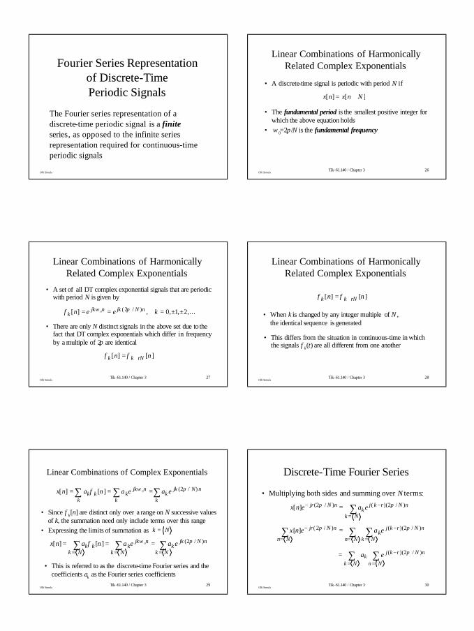
Ideal Frequency-Selective Filters• Ideal lowpass filter with cutoff frequency ω c

>

≤=

c

cjH

ωω

ωωω

||,0

||,1)(

1H(jω)

0−ωc ωc

PassbandStopband Stopband

ω

Olli Simula


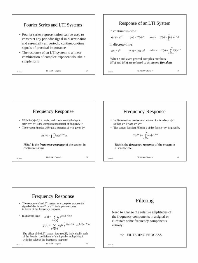
Ideal Frequency-Selective Filters• Ideal highpass filter with cutoff frequency ω c

≥

<=

c

cjH

ωω

ωωω

||,1

||,0)(

1H(jω)

0−ωc ωc

StopbandPassband Passband

ω


Ideal Frequency-Selective Filters• Ideal bandpass filter with cutoff frequencies ωc1 and ω c2

≤≤

=elsewhere

jHcc

,0

||,1)(

21 ωωωω

1

H(jω)

0ωc2−ωc2 −ωc1 ωc1 ω

Olli Simula




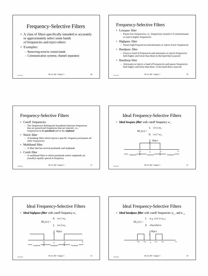
Ideal Frequency-Selective Filters• Ideal bandstop filter with cutoff frequencies ωc1 and ω c2

≤≤

=elsewhere

jHcc

,1

||,0)(

21 ωωωω

1H(jω)

0ωc2−ωc2 −ωc1 ωc1 ω


Ideal Frequency-Selective Filters• Each of these ideal continuous-time filters is symmetric

aboutω=0• There are two passbands for the highpass and bandpass

filters and three passbands for the bandstop filter

• Ideal discrete-time filters frequency-selective filters are defined in the similar way

• For discrete-time filters the frequency response is periodic with period 2π, with • Low frequencies near even multiples of π• High frequencies near odd multiples of π

Olli Simula


Ideal Discrete-Time Frequency-Selective Filters

• Lowpass

• Highpass

-2π 2π-π π ωωc−ωc 0

1

H(ejω)

-2π 2π-π π ωωc−ωc 0

1

H(ejω)


Ideal Discrete-Time Frequency-Selective Filters

• Bandpass

• Bandstop

-2π 2π-π π ω−ωc1−ωc2 0

1

H(ejω)

ωc2ωc

-2π 2π-π π ω−ωc1−ωc2 0

1

H(ejω)

ωc2ωc

Olli Simula


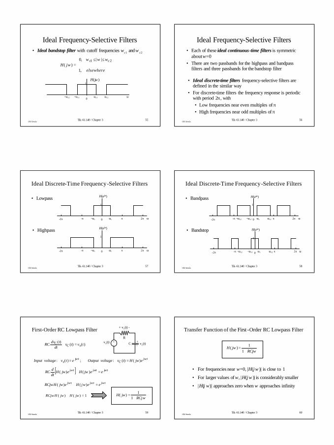
First-Order RC Lowpass Filter

+- C

R

+ v r(t) -

vs(t) vc(t)+-)()(

)(tvtv

dttdv

RC sCC =+

;)(: tjs etvvoltageInput ω= tj

C ejHtvvoltageOutput ωω)()(: =

[ ] tjtjtj eejHejHdtd

RC ωωω ωω =+ )()(

tjtjtj eejHejHRCj ωωω ωωω =+ )()(

1)()( =+ ωωω jHjHRCjω

ωRCj

jH+

=1

1)(


Transfer Function of the First -Order RC Lowpass Filter

ωω

RCjjH

+=

11)(

• For frequencies near ω=0, |H(j ω )| is close to 1

• For larger values of ω, |H(j ω )| is considerably smaller

• |H(j ω)| approaches zero when ω approaches infinity

Olli Simula




Transfer Function of the First -Order RC Lowpass Filter

• Impulse response: )(1

)( / tueRC

th RCt−=

• Step response: [ ] )(1)( / tuets RCt−−=

• Trade-offs in filter design:

– Narrow passband requirement: Large RC

– Fast step response: Small RC


First-Order RC Highpass Filter

+- C

R

+ v r(t) -

vs(t) vc(t)+-

)()()( tvtvtv RsC −=

• The output is now the voltage across the resistor

( ))()()(

)( tvtvdtd

Cdt

tdvCti Rs

C −==

−==dt

tdvdt

tdvRCtRitv Rs

R)()(

)()(

dttdv

RCtvdt

tdvRC s

RR )(

)()(

=+

Olli Simula


First-Order RC Highpass Filter

RCjRCj

jGω

ωω

+=

1)(

dttdv

RCtvdt

tdvRC s

RR )(

)()(

=+

;)(: tjs etvvoltageInput ω= tj

R ejGtvvoltageOutput ωω)()(: =

+- C

R

+ v r(t) -

vs(t) vc(t)+-

[ ] tjtjtj edtd

RCejGejGdtd

RC ωωω ωω =+ )()(

tjtjtj eRCjejGejGRCj ωωω ωωωω =+ )()(

ωωωω RCjjGjGRCj =+ )()(


Discrete-Time Filters Described by Constant Coefficient Difference Equations

• Discrete-time LTI systems described by difference equations can be either

Recursive and have an infinite impulse response (IIR systems)

orNonrecursive and have a finite impulse response (FIR systems)

• IIR systems are direct counterparts of continuous-time systems described by differential equations

Olli Simula


First-Order Recursive Discrete-Time Filters

ωω

jj

aeeH −−

=1

1)(

][]1[][ nxnayny =−−

++

DDa

][nx ][ny

]1[ −ny

;][: njenxInput ω=njj eeHnyOutput

ωω )(][: =

njnjjnjj eeeaHeeH ωωωωω =− − )1()()(

[ ] njnjjj eeeHae ωωωω =− − )(1

Difference equation:


Transfer Function of the First-Order Recursive Discrete-Time Filter

• Parameter a controls the behavior of the filter

• For a positive => Lowpass filter

a controls the rate of attenuation at low frequencies, ω=0

• For a negative => Highpass filter

a controls the rate of attenuation at high frequencies, ω=π

ωω

jj

aeeH −−

=1

1)(

Olli Simula




Transfer Function of the First-Order Recursive Discrete-Time Filter

• Impulse response: ][][ nuanh n=

• Step response:

• |a| controls the speed with which the impulse and step responses approach their long-term values,

With faster responses for smaller values of |a| , andhence for broader passbands

• For |a|<1 the system is stable, i.e., h[n] is absolutely summable

][][][ nhnuns ∗= ][1

1 1nu

aan

−−=

+


Nonrecursive Discrete-Time Filters

• General form of an FIR nonrecursive difference equation

∑−=

−=M

Nkk knxbny ][][

• The output is the weighted average of the (N+M+1) values of x[n] from x[n-M] through x[n+N] with the weights given by coefficients bk.

• Such a filter is often called a moving-average filter, where the output y[n] for any n , e.g. for n0 , is an average of values of x[n] in the vicinity of n0

Olli Simula


Three-Point Moving-Average Filter

• Difference equation

( )]1[][]1[31

][ +++−= nxnxnxny

• The impulse response

( )]1[][]1[31

][ +++−= nnnnh δδδ

• The frequency response

( )ωωω jjj eeeH ++= − 131

)( ( )ωcos2131

+=


Causal Three-Point Moving-Average Filter


( )]2[]1[][31

][ −+−+= nxnxnxny


( )]2[]1[][31

][ −+−+= nnnnh δδδ


( )ωωω 2131)( jjj eeeH −− ++=

( )ωω cos2131

+= − je

( )ωωω jjj eee −− ++= 131

Olli Simula


Three-Point Moving-Average Filter


General Moving-Average Filter


• The impulse response is a rectangular pulse, i.e.,h[n]=1/(N+M+1) for -N<n<M and h[n]=0 otherwise


[ ] [ ])2/sin(

2/)1(sin1

1)( 2/)(

ωωωω ++

++= − MN

eMN

eH MNjj

∑−=

−++

=M

Nkknx

MNny ][

11

][

Olli Simula




Moving-Average Filter with N+M+1=25


Moving-Average Filter with N+M+1=50

Olli Simula


Differentiating Nonrecursive Filter

• Consider the difference equation

( )2

]1[][][

−−=

nxnxny

• For input signals that vary greatly from sample to sample, the value of y[n] is large



( )ωω jj eeH −−= 121

)( )2/sin(2/ ωωjje −=

( )]1[][21

][ −−= nnnh δδ


First-Order Nonrecursive Highpass Filter

Olli Simula


Nonrecursive Discrete-Time Filters

• The impulse response of a nonrecursive FIR filter is of finite length

• The impulse response is, thus, always absolutely summable for any h[n]=bn

=> FIR filters are always stable

Olli Simula

Documents

Tik-61.140 Signal Processing Systems Spring 2001 Fourier Series ... · Tik-61.140 Signal Processing Systems Spring 2001 Chapter 3 / O. Simula 1 Fourier Series Representation of Continuous-Time