Embed Size (px)
Citation preview
HANDBOOKSAVANNA TOOLTIGER
Remote Sensing of Water Use and Water Stress in African Savanna Ecosystem from Local to Regional Scale
TIGER SAVANNA TOOLHANDBOOK:
On Remote Sensing of Water Use and Water Stress in African Savanna Ecosystems from Local to Regional Scale
Ana Andreu (UNU-FLORES)Eva Kimonye (UNU-FLORES)Timothy Dube (University of Limpopo)
Acknowledgements: The authors would like to thank Dr Nieto (IAS), Dr Guzinski (ESA), Dr González-Dugo (IFAPA), Tami Amudau (CSIR), Cleta Shoko (UKZN), Dr Abel Ramoelo (CSIR), Dr Stephan Hülsmann (UNU-FLORES), TIGER Capacity Building Facility and the European Space Agency for their support and contributions.
The views expressed in this publication are those of the authors.The authors are responsible for ensuring that all figures, tables, text, and supporting materials are properly cited and necessary permissions were obtained.
The authors would like to hear from you. Should you have any feedback for them, please reach out to Ana Andreu at [email protected] or [email protected], and / or Timothy Dube at [email protected].
United Nations University Institute for IntegratedManagement of Material Fluxes and of Resources(UNU-FLORES)
Ammonstrasse 74, 01067 Dresden, GermanyTel.: + 49-351 8921 9370Fax: + 49-351 8921 9389e-mail: [email protected]
© 2017 UNU-FLORESEditor: Atiqah Fairuz Salleh Design & Layout: diamonds network GmbHCover Image: Ana Andreu MendezFigures: UNU-FLORES or otherwise specified Print: Reprogress GmbHPrint run: 300
ISBN: 978-3-944863-54-2e-ISBN: 978-3-944863-55-9
This publication should be cited as:Ana Andreu, Eva Kimonye, and Timothy Dube. 2017. TIGER Savanna Tool Handbook: On Remote Sensing of Water Use and Water Stress in African Savanna Ecosystems from Local to Regional Scale. Dresden: United Nations University Institute for Integrated Management of Material Fluxes and of Resources (UNU-FLORES).
ABOUT UNU-FLORES
The United Nations University Institute for Integrated Management of Material Fluxes and of Resources (UNU-FLORES) based in Dresden, Germany contributes to the development of integrated and sustainable management strategies for the use of water, soil, and waste resources, particularly in developing and emerging countries in scientific, educational, managerial, technological, and institutional terms. UNU-FLORES hosts three research units that focus on the underlying resources of the nexus – water, soil, and waste – and two overarching units that look at systems and flux analysis under global change, and capacity development and governance.
ABOUT UKZN
The University of KwaZulu Natal (UKZN) in South Africa is an academic and research institution with four colleges: humanities, law and management studies, health sciences, and the College of Agriculture, Engineering and Science, which hosts the School of Agricultural, Earth and Environmental Sciences (SAEES). SAEES through the Earth Observation Unit, housed in the Geography Department, focuses on applications of Earth Observation technologies in ecosystems monitoring, land use and land cover, invasive species, mapping, water resources and environmental management, at both local and regional scales.

ABOUT IFAPA
The Andalusian Institute of Agricultural, Fisheries Research and Training (IFAPA) in Spain is a regional governmental institution focused on agricultural research, technology development, transfer and training. Its mission is to promote innovative actions to improve agricultural competitiveness, defined by regional, national, and international policies. IFAPA Alameda del Obispo is a leader in dehesa (productive Spanish oak savanna) management and conservation research, recognised by the Andalusian Regional Law (7/2010) as the coordinator and technical assistant of managers and policymakers in this area.
ABOUT THE TIGER INITIATIVE AND TIGER CBF
The TIGER initiative promotes the use of Earth Observation (EO) for improving Integrated Water Resources Management in Africa. The overall objective is to assist African countries to overcome problems faced in the collection, analysis, and use of water-related geo-information by exploiting the advantages of EO technology. The TIGER Capacity Building Facility (TCBF) is responsible for setting up a capacity building and training programme in support of the research under the TIGER initiative.
Funded by:European Space Agency (ESA), UNU-FLORES, and UKZN
guarantees end users’ freedom to run, study, share, and modify the tools. The development of an open-source Savanna Water Use and Water Stress Tool is essential to help improve rangeland resources management based on scientific evidence. In furthering the Nexus Approach, the integration of stakeholders’ perspectives within the framework of the project is promoted and Capacity Development actions reinforced.
2. The project focuses on safeguarding ecosystem services and livelihoods in Southern Africa, a region which is prone to water scarcity and where climatic change projections show that the ratio of temperatures/precipitation will progressively increase. This region has been a focus area of UNU-FLORES ever since its establishment in December 2012. The Institute started various initiatives in sub-Saharan Africa collaborating with a network of partners, among others addressing drought management.
3. TIGER project 410 supports the Sustainable Development Goals (SDGs), shaping and dominating the internal development agenda for the coming decades, with UNU-FLORES and UNU in general being deeply involved in activities related to monitoring and implementation. The project outcomes are particularly relevant for SDG 6 (Ensure availability and sustainable management of water and sanitation for all), SDG 13 (Take urgent action to combat climate change and its impacts by regulating emissions and promoting developments in renewable energy), and SDG 15 (Protect, restore and promote sustainable use of terrestrial ecosystems, sustainable manage forests, combat desertification, and halt and reverse land degradation and halt biodiversity loss), among other SDGs.
Overall, TIGER project 410 and in particular the tools introduced in this handbook are timely and pertinent considering the trends of global change. We hope that the TIGER tools will be taken up widely for resources management in African Savannas and developed further for additional applications in other regions.
Reza Ardakanian, DirectorStephan Hülsmann, Head of Unit, Systems and Flux Analysis considering Global Change Assessment
FOREWORD
Savannas are among Africa’s most productive multifunctional landscape – supporting wildlife, livestock, crops, and livelihoods – but experience frequent droughts, aggravated by climate change and other human-induced changes. To maintain ecosystem productivity while ensuring food security, we need to rely on an integrated management and monitoring of resources. Due to the interlinkages between resources, and between resources and society, their sustainable management requires a holistic perspective. This kind of integrated resources management has in recent years also be termed a Nexus Approach. At UNU-FLORES where advancing a Nexus Approach to the sustainable management of environmental resources is a main mission and focus, we seek to continuously develop tools to facilitate this development for stakeholders and practitioners.
In December 2015 UNU-FLORES, together with the University of Limpopo and the University of Western Cape (South Africa), were selected as one of the ten TIGER Water for Agriculture teams for conducting joint research for integrated water management, within project 410 “Remote Sensing of Water Use and Water Stress in African Savanna Ecosystem from Local to Regional Scale: Implications for Land Productivity”.
This project was considered highly relevant for advancing UNU-FLORES’s mission from three aspects:
1. An integrated management requires integrated tools, which are able to address and reduce uncertainties associated with resources management by the use of timely and precise information of ecosystem dynamics, in this case derived from Earth Observation data. Scientific open data sources are essential for monitoring ecosystems, especially in emerging countries with ground data scarcity, unreliable monitoring networks, and restricted data access. However, these data sources have to be homogenised and processed in order to derive information that can cover stakeholders’ needs.
Open-source software, like the Water Observation Information System (WOIS) developed by the TIGER Initiative, is valuable in this regard, since it

TABLE OF CONTENTS
1. Introduction . . . . . . . . . . . . . . . . . . . . . . . . . . . . . . . . . . . . . . . . . . . . . . . . . . . . . . . . . . . . . . . . . 2
Why Savannas Are Important . . . . . . . . . . . . . . . . . . . . . . . . . . . . . . . . . . . . . . . . . . . . . . . . . . . 2Why a Tool for Savannas? . . . . . . . . . . . . . . . . . . . . . . . . . . . . . . . . . . . . . . . . . . . . . . . . . . . . . . . 6
2. Our TIGER Project 410 . . . . . . . . . . . . . . . . . . . . . . . . . . . . . . . . . . . . . . . . . . . . . . . . . . . 7
3. Remote Sensing in Theory . . . . . . . . . . . . . . . . . . . . . . . . . . . . . . . . . . . . . . . . . . . . . 11
Earth Observation Techniques . . . . . . . . . . . . . . . . . . . . . . . . . . . . . . . . . . . . . . . . . . . . . . . . . 12Earth Observation Satellites Compilation . . . . . . . . . . . . . . . . . . . . . . . . . . . . . . . . 18European Space Agency and Copernicus Programme . . . . . . . . . . . . . . . . . 25
Measuring Evapotranspiration . . . . . . . . . . . . . . . . . . . . . . . . . . . . . . . . . . . . . . . . . . . . . . . . . 26Energy Balance and Micrometeorological Methods . . . . . . . . . . . . . . . . . . . . 27Measurement Methods Based on Soil-Water Balance . . . . . . . . . . . . . . . . . . 35Plant Physiology Approaches . . . . . . . . . . . . . . . . . . . . . . . . . . . . . . . . . . . . . . . . . . . . . . . 36
4. Tools in Practice . . . . . . . . . . . . . . . . . . . . . . . . . . . . . . . . . . . . . . . . . . . . . . . . . . . . . . . . . . . 39
TIGER Initiative and Water Observation and Information System . . . . . . . . 40Product Applications . . . . . . . . . . . . . . . . . . . . . . . . . . . . . . . . . . . . . . . . . . . . . . . . . . . . . . . . . . . . . 42
How To . . . . . . . . . . . . . . . . . . . . . . . . . . . . . . . . . . . . . . . . . . . . . . . . . . . . . . . . . . . . . . . . . . . . . . . . . . 43
References . . . . . . . . . . . . . . . . . . . . . . . . . . . . . . . . . . . . . . . . . . . . . . . . . . . . . . . . . . . . . . . . . . . . . . 51
Annexes . . . . . . . . . . . . . . . . . . . . . . . . . . . . . . . . . . . . . . . . . . . . . . . . . . . . . . . . . . . . . . . . . . . . . . . . . 63
LIST OF FIGURES
Fig. 1 Different vegetation layers in a savanna: tree, shrubs, and grasses in Kruger National Park of South Africa . . . . . . . . . . . . . . . . . . . . . 12Fig. 2 Map of South African biomes . . . . . . . . . . . . . . . . . . . . . . . . . . . . . . . . . . . . . . . . . . 14Fig. 3 Savanna regions ranging from Tropical, Subtropical, Temperate, Mediterranean, and Montane . . . . . . . . . . . . . . . . . . . . . . . . . . . . . . . . . . . . . . . . . . . 15Fig. 4 Modelling savanna ecosystem with Sentinel data . . . . . . . . . . . . . . . . . . . 18Fig. 5 Study area where the savanna tool was tested and validated . . . . . 19Fig. 6 EO scheme for gathering and processing information . . . . . . . . . . . . . 22Fig. 7 Atmospheric windows for satellites . . . . . . . . . . . . . . . . . . . . . . . . . . . . . . . . . . . . 23Fig. 8 Different satellite orbits – polar orbit at different speed from the Earth, and geostationary orbit at the same speed as the Earth . . . 24Fig. 9 Spatial, spectral, and temporal resolution . . . . . . . . . . . . . . . . . . . . . . . . . . . . 25Fig. 10 Main applications of each spectral region . . . . . . . . . . . . . . . . . . . . . . . . . . . . 26Fig. 11 Earth Observation satellites . . . . . . . . . . . . . . . . . . . . . . . . . . . . . . . . . . . . . . . . . . . . 27Fig. 12 Sentinel satellites . . . . . . . . . . . . . . . . . . . . . . . . . . . . . . . . . . . . . . . . . . . . . . . . . . . . . . . . . 33Fig. 13 (a) Evapotranspiration process . . . . . . . . . . . . . . . . . . . . . . . . . . . . . . . . . . . . . . . . . 34Fig. 13 (b) Factors determining transpiration . . . . . . . . . . . . . . . . . . . . . . . . . . . . . . . . . 34Fig. 14 Surface energy balance fluxes scheme . . . . . . . . . . . . . . . . . . . . . . . . . . . . . . . 35Fig. 15 (a) Scintillometer located in Las Tiesas experimental farm . . . . . . . . 36Fig. 15 (b) Eddy covariance tower (ECT) system located in Skukuza, South Africa . . . . . . . . . . . . . . . . . . . . . . . . . . . . . . . . . . . . . . . . . . . . . . . . . . . . . . . . . . . . . . . 36Fig. 16 Eddy covariance tower system scheme . . . . . . . . . . . . . . . . . . . . . . . . . . . . . . . 37Fig. 17 Footprint contribution area scheme . . . . . . . . . . . . . . . . . . . . . . . . . . . . . . . . . . . 38Fig. 18 Distribution of tower sites in the global network of networks . . . . . 39Fig. 19 TIGER Initiative presence in Africa . . . . . . . . . . . . . . . . . . . . . . . . . . . . . . . . . . . . . 44Fig. 20 TIGER Initiative tools and objectives . . . . . . . . . . . . . . . . . . . . . . . . . . . . . . . . . . 45Fig. 21 ETo and crop coefficient method . . . . . . . . . . . . . . . . . . . . . . . . . . . . . . . . . . . . . . . 61Fig. 22 Energy balance scheme of TSEB model and equation . . . . . . . . . . . . . 65
SYMBOLS
A ............. Maximum value of the ratio G/RnSB ............ Soil heat flux calculation constantET0 .......... Reference evapotranspirationF ............. PhotosynthesisƒC ............. Fractional ground coverƒg ............. Green vegetation fractionFx' ........... Relative contribution per running metre along the wind directionFx'y' .......... Source strength for the footprint modelG ............. Soil heat fluxH ............. Sensible heat fluxhC ............ Canopy heightHc ............ Canopy sensible heat fluxHs ............ Soil sensible heat fluxk ............. Leaf angle distribution functionk' ............. Damping coefficientKcb ........... Basal crop coefficientKe ............ Evaporation crop coefficientKs ............ Water stress coefficientLE ........... Latent heat fluxLEC .......... Canopy latent heat fluxLES .......... Soil latent heat fluxNIR ......... Near infrared part of the spectrump' ............. Empirical parameter defined to computed fcPR ........... PrecipitationR ............. Surface runoffRA ............ Aerodynamic resistanceRn ........... Net radiationRnC .......... Net radiation reaching the canopyRnS .......... Net radiation reaching the soilRS ........... Resistance to the heat flow in the boundary layer above the soil RX ............ Resistance to heat flow of the vegetation leaf boundary layer S ............. Energy storage within the biomass
s' ............. Instantaneous fluctuations of the state variableSdn .......... Incoming solar radiation SWIR ....... Medium-infrared part of the spectrumt .............. Time intervalT' ............ Instantaneous fluctuations of the air temperatureT0 ............ Aerodynamical temperatureTAC .......... Air temperature in the canopy – air space Tair .......... Air temperature above the canopyTC ............ Canopy temperatureTIR .......... Thermal part of the spectrumTRAD ......... Radiometric surface temperaturetS ............. Time in seconds relative to solar noonu(z) ......... Wind speed at height zVI ............ Vegetation indexVIS .......... Visible part of the spectrumw' ............ Instantaneous fluctuations of the vertical wind speedαPT .......... Priestley-Taylor coefficientϕ ............. Viewing angle
1. INTRODUCTION
32 32
WHY SAVANNAS ARE IMPORTANT
Savannas are among the most complex, variable, and extensive biomes on Earth (Scholes and Walker 2004; Beerling and Osborne 2006), covering half of Africa (Sankaran and Ratnam 2013). Approximately one fifth of the world population live in or around savannas (Asner et al. 2015). Savannas support wildlife, livestock, rangelands, crops, and livelihoods (Scholes and Archer 1997), playing an important socioeconomic role in rural areas. Most of the world’s savannas are found in Africa, with smaller concentrations in India, Australia, America, and Europe (Wilgen 2010; Papanastasis 2004).
Savannas provide valuable ecosystem services at local, regional, and global scales (Kamaljit 2006). These multifunctional uses include grazing for meat production, recreation and tourism, sites for educational and research studies, preservation of indigenous culture, and land use for agriculture. Savanna ecosystem stability has a great influence in global land-surface processes and Earth water and carbon cycles, maintaining biodiversity, improving soil fertility, and maintaining regional hydrological balance (Kamaljit 2006).
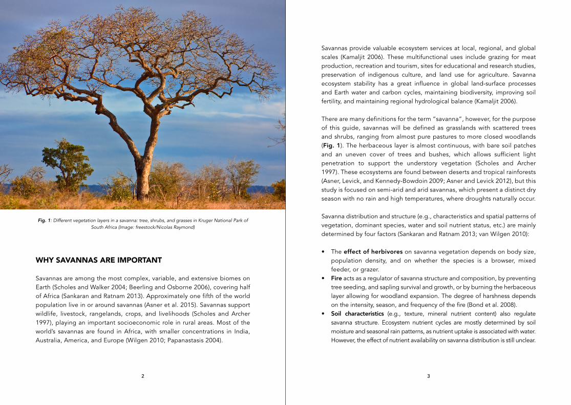
There are many definitions for the term “savanna”, however, for the purpose of this guide, savannas will be defined as grasslands with scattered trees and shrubs, ranging from almost pure pastures to more closed woodlands (Fig. 1). The herbaceous layer is almost continuous, with bare soil patches and an uneven cover of trees and bushes, which allows sufficient light penetration to support the understory vegetation (Scholes and Archer 1997). These ecosystems are found between deserts and tropical rainforests (Asner, Levick, and Kennedy-Bowdoin 2009; Asner and Levick 2012), but this study is focused on semi-arid and arid savannas, which present a distinct dry season with no rain and high temperatures, where droughts naturally occur.
Savanna distribution and structure (e.g., characteristics and spatial patterns of vegetation, dominant species, water and soil nutrient status, etc.) are mainly determined by four factors (Sankaran and Ratnam 2013; van Wilgen 2010):
• The effect of herbivores on savanna vegetation depends on body size, population density, and on whether the species is a browser, mixed feeder, or grazer.
• Fire acts as a regulator of savanna structure and composition, by preventing tree seeding, and sapling survival and growth, or by burning the herbaceous layer allowing for woodland expansion. The degree of harshness depends on the intensity, season, and frequency of the fire (Bond et al. 2008).
• Soil characteristics (e.g., texture, mineral nutrient content) also regulate savanna structure. Ecosystem nutrient cycles are mostly determined by soil moisture and seasonal rain patterns, as nutrient uptake is associated with water. However, the effect of nutrient availability on savanna distribution is still unclear.
Fig. 1: Different vegetation layers in a savanna: tree, shrubs, and grasses in Kruger National Park of South Africa (Image: freestock/Nicolas Raymond)

54 4
• Water availability, influenced by annual rainfall, soil infiltration capacity, evapotranspiration, soil texture, and the hydrological regime, plays a critical role in defining savanna ecology and structure.
These water-limited ecosystems with seasonal water availability are highly sensitive to changes in both climate conditions and in land-use/management practices (Schnabel, Dahlgren, and Moreno 2013; IPCC 2014; Kueppers et al. 2005; Bond et al. 2008), and water scarcity situations have been aggravated by global warming. These changes are modifying not only their structure, affecting the ecosystem's long-term functioning (Baldocchi and Xu 2007), but also the land-atmosphere linkages and the regional water and carbon cycles, in ways still unknown (Jeltsch, Weber, and Grimm 2000; Bond and Keeley 2005). Most significant threats, caused by anthropogenic factors, are:
• Fires provoked by human activity, which make the original canopy recovery difficult.
• Agriculture and livestock farming adding pressure to savanna ecological status, with overgrazing interfering with vegetation and soil structure (e.g., compaction, soil erosion, etc).
• Resources overexploitation (timber, herbs, mushrooms, etc.), indiscriminate hunting, over-extraction of fuel and minerals, etc.
In South Africa, where the study was conducted and remote sensing tool tested, savannas cover about a third of the land area (Wilgen 2010), providing two vital services: wildlife-related tourism and cattle ranching. It is estimated that around 9.2 million of South Africans benefit directly from these ecosystem services, through the use of resources.
Savannas occupy the northern, southern, and eastern part of the country (Fig. 2), with arid savannas extending to the southern Kalahari. They have different climatic and ecological characteristics, being defined according to their prominent canopy layer: shrubveld if the upper vegetation is near ground level and bushveld if characterised by dense and tall vegetation (Asner et al.
2015). According to Asner et al (2016), summer rainfall is essential for South African savannas, and fires are the major factor shaping their structure.
Fig. 2: Map of South African biomes(based on BGIS by SANBI- South African National Biodiversity Institute)
Since savannas are highly influenced by human activities, private and institutional practices play a key role in their conservation, improving people’s living standards and providing employment opportunities. There is a need to develop a mechanism for monitoring water availability and vegetation dynamics in savannas, at both the regional and local scales.
5
6
2. OUR TIGER PROJECT 410
WHY A TOOL FOR SAVANNAS?
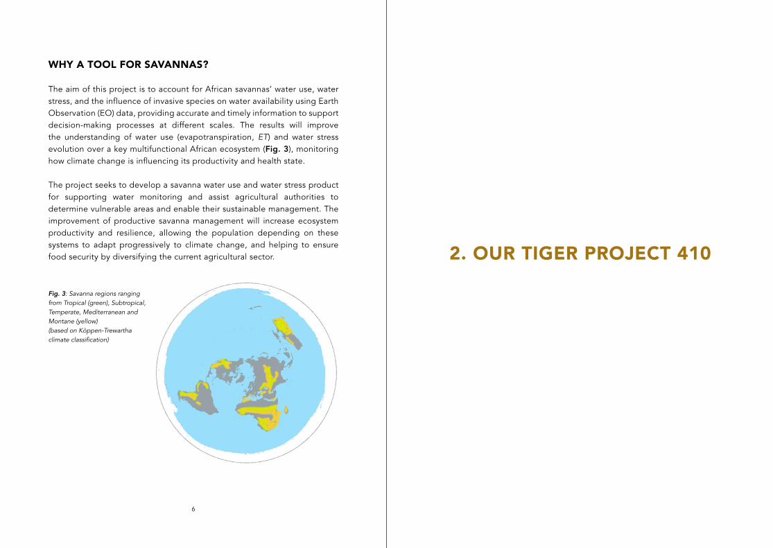
The aim of this project is to account for African savannas’ water use, water stress, and the influence of invasive species on water availability using Earth Observation (EO) data, providing accurate and timely information to support decision-making processes at different scales. The results will improve the understanding of water use (evapotranspiration, ET) and water stress evolution over a key multifunctional African ecosystem (Fig. 3), monitoring how climate change is influencing its productivity and health state.
The project seeks to develop a savanna water use and water stress product for supporting water monitoring and assist agricultural authorities to determine vulnerable areas and enable their sustainable management. The improvement of productive savanna management will increase ecosystem productivity and resilience, allowing the population depending on these systems to adapt progressively to climate change, and helping to ensure food security by diversifying the current agricultural sector.
Fig. 3: Savanna regions ranging from Tropical (green), Subtropical, Temperate, Mediterranean and Montane (yellow)(based on Köppen-Trewartha climate classification)
98
Savannas are among Africa’s most productive landscapes, supporting livestock, crops, and livelihoods (Mbatha and Ward 2010). This ecosystem experiences frequent droughts, aggravated by climate change and other human-induced changes, such as invasive species, with severe implications on the regional water balance, biodiversity, and agricultural productivity. Although monitoring programmes for savanna water use have been established in certain areas, these are largely restricted to point-based/small scales, not providing timely distributed information for planning purposes.
The Earth Observation (EO) data provided by Sentinel 2’s and Sentinel 3’s new missions will allow us to map the water use/stress and the invasive species distribution across the African savannas (Fig. 4), as well as to monitor seasonal and long-term temporal variations.
To monitor savanna ecosystem water use/stress in a semi-continuous spatio-temporal way, this project integrates two different ET-estimation approaches, with different conceptual/operational capabilities and limitations. Kc-FAO56 (Allen et al. 1998), integrating reflectance-based “crop” coefficients, is used to derive unstressed savanna evapotranspiration (with high spatial resolution), and the two-source surface energy balance model (TSEB) (Norman, Kustas, and Humes 1995) integrating radiometric surface temperature allows the determination of water stress across savannas (with low spatial resolution).
The choice of the two approaches is based on their proven ability to estimate ET over partially vegetated heterogeneous landscapes (Cammalleri et al. 2010; Gonzalez-Dugo et al. 2009), as well as over savanna-type ecosystems (Andreu et al. 2013; Campos et al. 2013).
This procedure was tested over eddy covariance experimental sites in South Africa (Fig. 5), using different satellite data sets (during 2011–2012: SPOT 5 MS & AATSR, since June 2015: Sentinel 2 MSI & MODIS/Sentinel 3A SLSTR). The high spatial resolution of visible and near infrared (VIS/NIR) data and the vegetation’s different spectral response will be used to precisely map water use and stress over the savanna.
Fig. 4: Modelling savanna ecosystem with Sentinel data
Fig. 5: Study area where the savanna tool was tested and validated
3. REMOTE SENSING IN THEORY
1312
EARTH OBSERVATION TECHNIQUES
Nowadays, remote observation techniques of the Earth’s surface have become an essential tool to support decision-making processes (and policy recommendations) in many sectors, such as agriculture, forestry, weather forecasting, or land-use policy (Alcaraz-Segura 2014). Earth Observation (EO) data characteristics – global coverage, with various temporal (hourly, weekly, bi-weekly) and spatial (metres to tens of kilometres) resolutions; non-destructive nature; immediate transmission, digital format, and the open accessibility of some of them (e.g., Sentinels mission from the European Space Agency, or Landsat series and MODIS missions from NASA) – make them essential to evaluate ecosystems functioning in developing countries, due to ground data scarcity, unreliable monitoring networks, lack of data access, and, in some cases, lack of technical expertise (Sheffield et al. 2014).
Fig. 6: EO scheme for gathering and processing information
However, the existence of these data sources has not necessarily resulted in benefits for society. They have to be processed and analysed, sometimes using complex statistical approaches and modelling techniques, in order to derive information that can be used by stakeholders.
Between the surface and sensor there is an energy interaction, either due to the solar energy reflectance (visible-VIS and near infrared-NIR), an artificial energy beam reflectance (radar systems), or by self-emission of the surface (thermal/microwave). Signals are transmitted through the atmosphere and captured by the sensors, finally available for further processing in digital format (Fig. 6). The energy flux between the surface and the sensor takes the form of electromagnetic radiation and is defined by its wavelength and frequency. Although the electromagnetic spectrum is continuous, the detectors need to divide it into a number of bands within which the radiation shows similar behaviour.
The most frequently used regions in remote sensing are the visible part of the spectrum (VIS, 0.4–0.7 μm) and the near-infrared (NIR, 0.7–1.3 μm), useful for discriminating canopy masses and humidity; medium-infrared (SWIR, 1.3–3 μm), where reflectance of solar energy and emissivity from the surface are shown together; thermal (TIR, 3–100 μm), which includes the emissivity portion of the spectrum in terms of ground cover temperature; and microwave bands (1 mm–1 m), radiation that can penetrate clouds.
The reflectance is the proportion of the incident energy reflected by a surface, a dimensionless magnitude that ranges between 0 and 1. For a given surface, it varies depending on the wavelength, and the curve representing this variation is called the spectral signature. This spectrum is characteristic of each surface and state, and enables land uses, materials, canopy growth status, etc., to be discriminated and classified (Richards and Jia 2006).
When the electromagnetic radiation passes through the atmosphere it is attenuated by absorption and dispersion processes. The absorption is defined as the transformation that the energy undergoes when it passes
1514
through a medium. A fraction of the energy is absorbed by the atmospheric components (O2, CO2, O3, and water vapour) and emitted at different wavelengths.
Satellites used in remote sensing are designed to operate outside the regions where absorption effects are greatest, in what are called atmospheric windows (Fig. 7). The dispersion process produces a change in the direction of a portion of the incidence radiation in relation to the original one, due to the interaction between the energy and the suspended atmospheric particles. To avoid the effects of these processes in the analysis it is necessary to correct the original data acquired by the sensor using various methods, according to the part of the spectrum of interest (Gordon and Morel 1983; Saunders and Kriebel 1988; Asrar, Kanemasu, and Yoshida 1985; Lenoble 1993; Kaufman and Sendra 1988).
Sensors mounted on satellites follow an orbit around the Earth depending on the objectives and characteristics of their mission. In general, orbits are defined by their height, orientation, and rotation relative to the Earth. Geostationary orbits are located at altitudes of around 36,000 km, always seeing the same portion of the globe because they replicate the angular speed of the Earth (e.g., meteorological satellites such as METEOSAT or GOES).
Fig. 7: Atmospheric windows for satellites (figure adapted from Casey, Kääb, and Benn 2012)
Most of the satellites are in polar orbit, covering the same portion of the surface at a fixed daily time, thus ensuring similar light conditions for the information they acquire (Fig. 8). In their movement around the Earth the satellites cover a given area of the surface, with the swath width depending on the satellite’s field of view (FOV) and the pixel size on the sensor’s instantaneous field of view (IFOV).
The resolution of a sensor is given by its ability to register and discriminate information, and it is dependent on the combined effect of a number of
Fig. 8: Different satellite orbits – polar orbit at different speed from the Earth, and geostationary orbit at the same speed as the Earth
1716
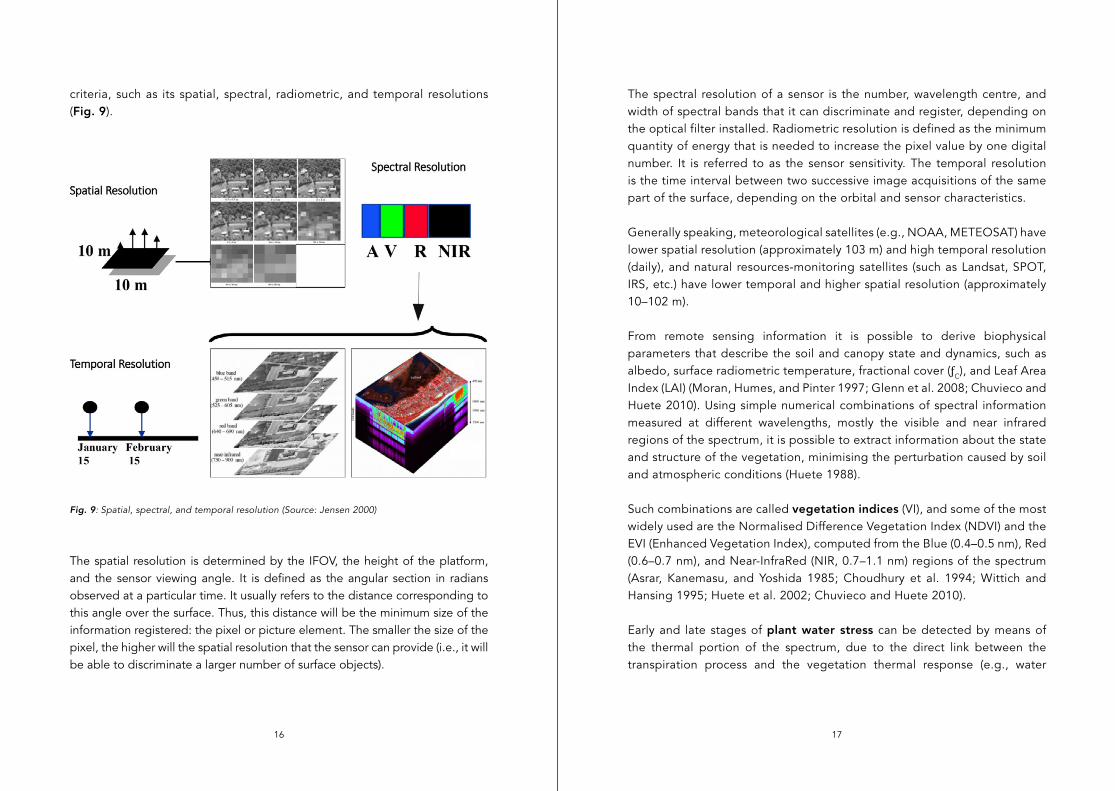
criteria, such as its spatial, spectral, radiometric, and temporal resolutions (Fig. 9).
The spatial resolution is determined by the IFOV, the height of the platform, and the sensor viewing angle. It is defined as the angular section in radians observed at a particular time. It usually refers to the distance corresponding to this angle over the surface. Thus, this distance will be the minimum size of the information registered: the pixel or picture element. The smaller the size of the pixel, the higher will the spatial resolution that the sensor can provide (i.e., it will be able to discriminate a larger number of surface objects).
The spectral resolution of a sensor is the number, wavelength centre, and width of spectral bands that it can discriminate and register, depending on the optical filter installed. Radiometric resolution is defined as the minimum quantity of energy that is needed to increase the pixel value by one digital number. It is referred to as the sensor sensitivity. The temporal resolution is the time interval between two successive image acquisitions of the same part of the surface, depending on the orbital and sensor characteristics.
Generally speaking, meteorological satellites (e.g., NOAA, METEOSAT) have lower spatial resolution (approximately 103 m) and high temporal resolution (daily), and natural resources-monitoring satellites (such as Landsat, SPOT, IRS, etc.) have lower temporal and higher spatial resolution (approximately 10–102 m).
From remote sensing information it is possible to derive biophysical parameters that describe the soil and canopy state and dynamics, such as albedo, surface radiometric temperature, fractional cover (ƒC), and Leaf Area Index (LAI) (Moran, Humes, and Pinter 1997; Glenn et al. 2008; Chuvieco and Huete 2010). Using simple numerical combinations of spectral information measured at different wavelengths, mostly the visible and near infrared regions of the spectrum, it is possible to extract information about the state and structure of the vegetation, minimising the perturbation caused by soil and atmospheric conditions (Huete 1988).
Such combinations are called vegetation indices (VI), and some of the most widely used are the Normalised Difference Vegetation Index (NDVI) and the EVI (Enhanced Vegetation Index), computed from the Blue (0.4–0.5 nm), Red (0.6–0.7 nm), and Near-InfraRed (NIR, 0.7–1.1 nm) regions of the spectrum (Asrar, Kanemasu, and Yoshida 1985; Choudhury et al. 1994; Wittich and Hansing 1995; Huete et al. 2002; Chuvieco and Huete 2010).
Early and late stages of plant water stress can be detected by means of the thermal portion of the spectrum, due to the direct link between the transpiration process and the vegetation thermal response (e.g., water
Fig. 9: Spatial, spectral, and temporal resolution (Source: Jensen 2000)
1918
evaporation from the leaves to the atmosphere cools the plant (Idso and Baker 1967). Transpiration strongly affects the proper functioning of these systems, and a reduction in the vegetation water content has an impact on the growth of plants and their physiological functions (Hatfield 1997). Thus, with the launch of satellite-based thermal sensors, TIR information, capable of continuous distributed monitoring of the health of ecosystems, is available.
Earth Observation Satellites Compilation
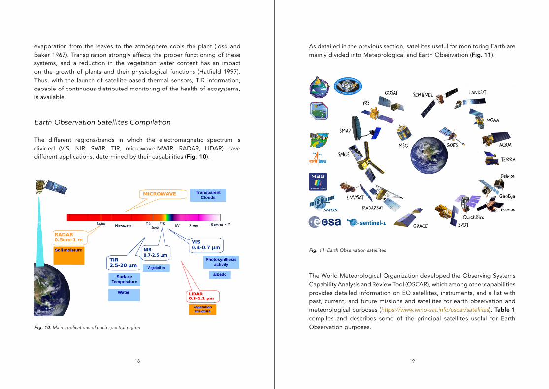
The different regions/bands in which the electromagnetic spectrum is divided (VIS, NIR, SWIR, TIR, microwave-MWIR, RADAR, LIDAR) have different applications, determined by their capabilities (Fig. 10).
Fig. 10: Main applications of each spectral region
As detailed in the previous section, satellites useful for monitoring Earth are mainly divided into Meteorological and Earth Observation (Fig. 11).
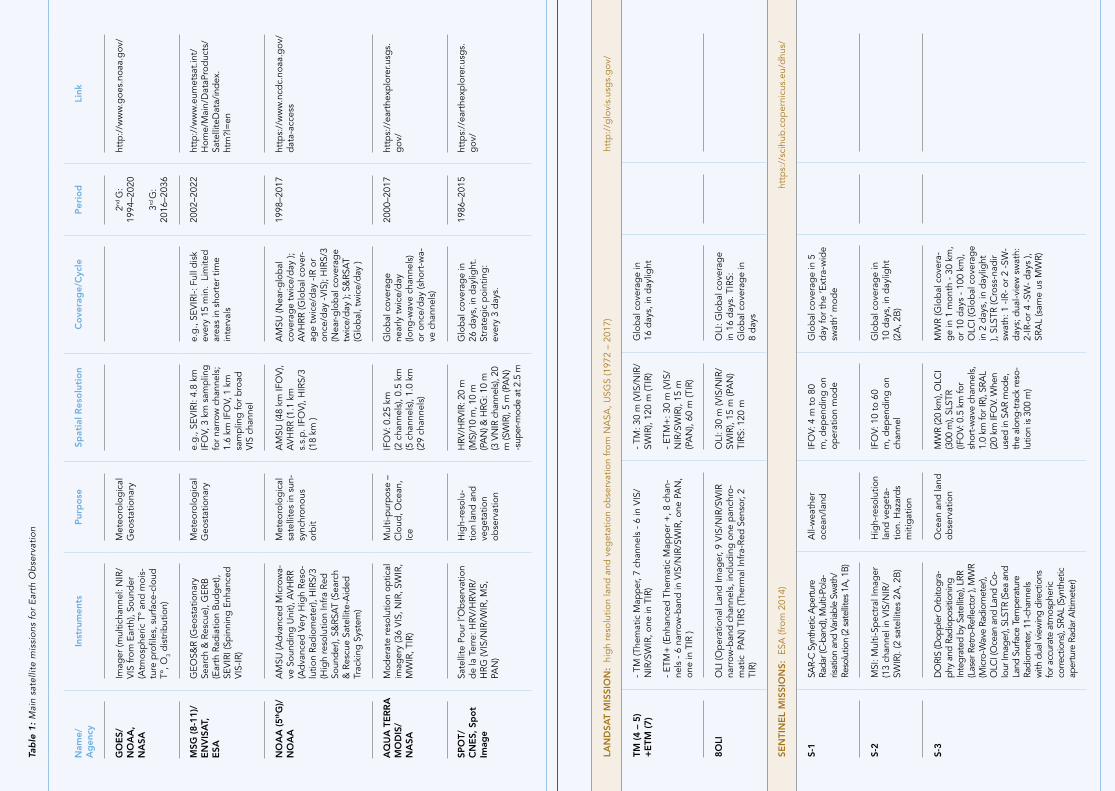
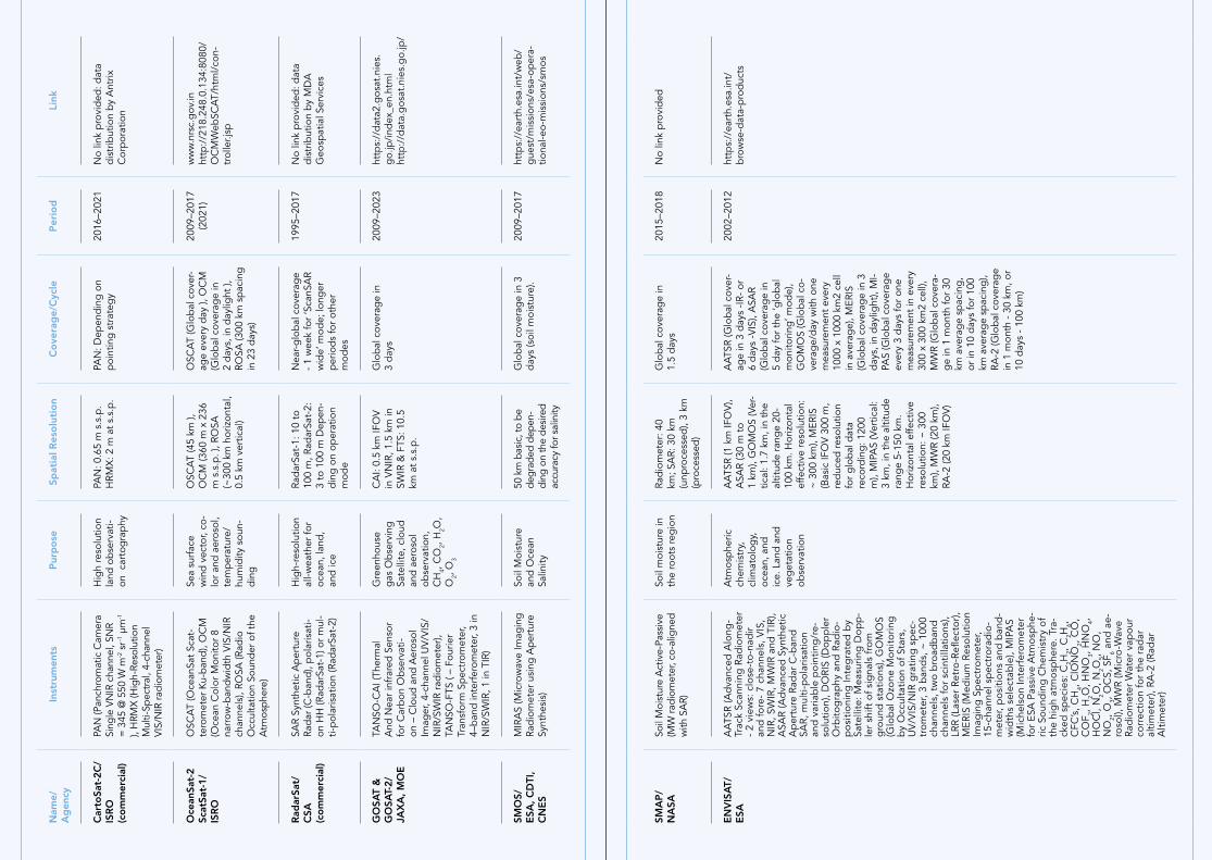
The World Meteorological Organization developed the Observing Systems Capability Analysis and Review Tool (OSCAR), which among other capabilities provides detailed information on EO satellites, instruments, and a list with past, current, and future missions and satellites for earth observation and meteorological purposes (https://www.wmo-sat.info/oscar/satellites). Table 1 compiles and describes some of the principal satellites useful for Earth Observation purposes.
Fig. 11: Earth Observation satellites
2120
Tab
le 1
: M
ain
sate
llite
mis
sio
ns f
or
Ear
th O
bse
rvat
ion
Nam
e/A
gen
cyIn
stru
men
tsP
urp
ose
Spat
ial R
eso
luti
on
Co
vera
ge/
Cyc
leP
erio
dLi
nk
GO
ES/
NO
AA
,N
ASA
Imag
er (m
ultic
hann
el: N
IR/
VIS
from
Ear
th),
Soun
der
(A
tmos
phe
ric T
° an
d m
ois-
ture
pro
files
, sur
face
-clo
ud
T°, O
3 dis
trib
utio
n)
Met
eoro
log
ical
Geo
stat
iona
ry2nd
G:
1994
–202
0
3rd G
: 20
16–2
036
http
://w
ww
.goe
s.no
aa.g
ov/
MSG
(8-1
1)/
EN
VIS
AT,
E
SA
GEO
S&R
(Geo
stat
iona
ry
Sear
ch &
Res
cue)
, GER
B
(Ear
th R
adia
tion
Bud
get
), SE
VIR
I (Sp
inni
ng E
nhan
ced
V
IS-IR
)
Met
eoro
log
ical
Geo
stat
iona
ry
e.g
., SE
VIR
I: 4.
8 km
IF
OV,
3 k
m s
amp
ling
fo
r na
rrow
cha
nnel
s;
1.6
km IF
OV,
1 k
m
sam
plin
g fo
r b
road
V
IS c
hann
el
e.g
., SE
VIR
I-: F
ull d
isk
ever
y 15
min
. Li
mite
d
area
s in
sho
rter
tim
e in
terv
als
2002
–202
2
http
://w
ww
.eum
etsa
t.in
t/H
ome/
Mai
n/D
ata P
rod
ucts
/ Sa
telli
teD
ata/
ind
ex.
htm
?l=
en
NO
AA
(5thG
)/N
OA
AA
MSU
(Ad
vanc
ed M
icro
wa-
ve S
ound
ing
Uni
t), A
VH
RR
(Ad
vanc
ed V
ery
Hig
h Re
so-
lutio
n Ra
dio
met
er),
HIR
S/3
(Hig
h re
solu
tion
Infr
a Re
d
Soun
der
), S&
RSA
T (S
earc
h &
Res
cue
Sate
llite
-Aid
ed
Trac
king
Sys
tem
)
Met
eoro
log
ical
sa
telli
tes
in s
un-
sync
hron
ous
orb
it
AM
SU (4
8 km
IFO
V),
AV
HRR
(1.1
km
s.
s.p
. IFO
V),
HIR
S/3
(18
km )
AM
SU (N
ear-
glo
bal
co
vera
ge
twic
e/d
ay );
A
VH
RR (G
lob
al c
over
-ag
e tw
ice/
day
-IR
or
once
/day
-V
IS);
HIR
S/3
(Nea
r-g
lob
al c
over
age
twic
e/d
ay );
S&
RSA
T (G
lob
al, t
wic
e/d
ay )
1998
–201
7
http
s://
ww
w.n
cdc.
noaa
.gov
/d
ata-
acce
ss
AQ
UA
TE
RR
A
MO
DIS
/N
ASA
Mod
erat
e re
solu
tion
optic
al
imag
ery
(36
VIS
, NIR
, SW
IR,
MW
IR, T
IR)
Mul
ti-p
urp
ose
– C
loud
, Oce
an,
Ice
IFO
V: 0
.25
km(2
cha
nnel
s), 0
.5 k
m
(5 c
hann
els)
, 1.0
km
(2
9 ch
anne
ls)
Glo
bal
cov
erag
e ne
arly
tw
ice/
day
(lo
ng-w
ave
chan
nels
) or
onc
e/d
ay (s
hort
-wa-
ve c
hann
els)
2000
–201
7
http
s://
eart
hexp
lore
r.usg
s.g
ov/
SPO
T/C
NE
S, S
po
t Im
age
Sate
llite
Pou
r l’O
bse
rvat
ion
de
la T
erre
: HRV
/HRV
IR/
HRG
(VIS
/NIR
/WIR
, MS,
PA
N)
Hig
h-re
solu
-tio
n la
nd a
nd
veg
etat
ion
obse
rvat
ion
HRV
/HRV
IR: 2
0 m
(M
S)/1
0 m
, 10
m
(PA
N) &
HRG
: 10
m
(3 V
NIR
cha
nnel
s), 2
0 m
(SW
IR),
5 m
(PA
N)
-sup
er-m
ode
at 2
.5 m
Glo
bal
cov
erag
e in
26
day
s, in
day
light
. St
rate
gic
poi
ntin
g:
ever
y 3
day
s.
1986
–201
5ht
tps:
//ea
rthe
xplo
rer.u
sgs.
gov
/
LAN
DSA
T M
ISSI
ON
: h
igh
reso
lutio
n la
nd a
nd v
eget
atio
n ob
serv
atio
n fr
om N
ASA
, USG
S (1
972
– 20
17)
http
://g
lovi
s.us
gs.
gov
/
TM (4
– 5
)+
ETM
(7)
- TM
(The
mat
ic M
app
er, 7
cha
nnel
s -
6 in
VIS
/N
IR/S
WIR
, one
in T
IR)
- ET
M+
(Enh
ance
d T
hem
atic
Map
per
+, 8
cha
n-ne
ls -
6 n
arro
w-b
and
in V
IS/N
IR/S
WIR
, one
PA
N,
one
in T
IR )
- TM
: 30
m (V
IS/N
IR/
SWIR
), 12
0 m
(TIR
)
- ET
M+
: 30
m (V
IS/
NIR
/SW
IR),
15 m
(P
AN
), 60
m (T
IR)
Glo
bal
cov
erag
e in
16 d
ays,
in d
aylig
ht
8OLI
OLI
(Op
erat
iona
l Lan
d Im
ager
, 9 V
IS/N
IR/S
WIR
na
rrow
-ban
d c
hann
els,
incl
udin
g o
ne p
anch
ro-
mat
ic P
AN
) TIR
S (T
herm
al In
fra-
Red
Sen
sor,
2 TI
R)
OLI
: 30
m (V
IS/N
IR/
SWIR
), 15
m (P
AN
) TI
RS: 1
20 m
OLI
: Glo
bal
cov
erag
e in
16
day
s. T
IRS:
G
lob
al c
over
age
in
8 d
ays
SEN
TIN
EL
MIS
SIO
NS:
ES
A (f
rom
201
4)
http
s://
scih
ub.c
oper
nicu
s.eu
/dhu
s/
S-1
SAR-
C S
ynth
etic
Ape
rture
Ra
dar (
C-b
and)
, Mul
ti-Po
la-
risat
ion
and
Varia
ble
Swat
h/Re
solu
tion
(2 s
atel
lites
1A
, 1B)
All-
wea
ther
oc
ean/
land
IFO
V: 4
m t
o 80
m
, dep
end
ing
on
oper
atio
n m
ode
Glo
bal
cov
erag
e in
5
day
for
the
‘Ext
ra-w
ide
swat
h’ m
ode
S-2
MSI
: Mul
ti-Sp
ectr
al Im
ager
(1
3 ch
anne
l in
VIS
/NIR
/SW
IR).
(2 s
atel
lites
2A
, 2B
)
Hig
h-re
solu
tion
land
veg
eta-
tion.
Haz
ard
s m
itig
atio
n
IFO
V: 1
0 to
60
m, d
epen
din
g o
n ch
anne
l
Glo
bal
cov
erag
e in
10
day
s, in
day
light
(2
A, 2
B)
S-3
DO
RIS
(Dop
pler
Orb
itogr
a-ph
y an
d Ra
diop
ositi
onin
g
Inte
grat
ed b
y Sa
telli
te),
LRR
(Las
er R
etro
-Refl
ecto
r ), M
WR
(Mic
ro-W
ave
Radi
omet
er),
OLC
I (O
cean
and
Lan
d C
o-lo
ur Im
ager
), SL
STR
(Sea
and
La
nd S
urfa
ce T
empe
ratu
re
Radi
omet
er, 1
1-ch
anne
ls
with
dua
l vie
win
g di
rect
ions
fo
r acc
urat
e at
mos
pher
ic
corre
ctio
ns),
SRA
L (S
ynth
etic
ap
ertu
re R
adar
Alti
met
er)
Oce
an a
nd la
nd
obse
rvat
ion
MW
R (2
0 km
), O
LCI
(300
m),
SLST
R (IF
OV:
0.5
km
for
shor
t-w
ave
chan
nels
, 1.
0 km
for I
R), S
RAL
(20
km IF
OV.
Whe
n us
ed in
SA
R m
ode,
th
e al
ong-
trac
k re
so-
lutio
n is
300
m)
MW
R (G
lob
al c
over
a-g
e in
1 m
onth
- 3
0 km
, or
10
day
s -
100
km),
OLC
I (G
lob
al c
over
age
in 2
day
s, in
day
light
),
SLST
R (C
ross
-nad
ir sw
ath:
1 -
IR-
or 2
-SW
- d
ays;
dua
l-vie
w s
wat
h:
2-IR
-or
4 -S
W-
day
s ),
SRA
L (s
ame
us M
WR)
2322
Nam
e/A
gen
cyIn
stru
men
tsP
urp
ose
Spat
ial R
eso
luti
on
Co
vera
ge/
Cyc
leP
erio
dLi
nk
Car
toSa
t-2C
/IS
RO
(co
mm
erci
al)
PAN
(Pan
chro
mat
ic C
amer
a Si
ngle
VN
IR c
hann
el, S
NR
= 3
45 @
550
W m
-2 s
r -1 µ
m-1
), H
RMX
(Hig
h-Re
solu
tion
Mul
ti-Sp
ectr
al, 4
-cha
nnel
VI
S/N
IR ra
diom
eter
)
Hig
h re
solu
tion
land
ob
serv
ati-
on c
arto
gra
phy
PAN
: 0.6
5 m
s.s
.p.
HRM
X: 2
m a
t s.
s.p
. PA
N: D
epen
din
g o
n p
oint
ing
str
ateg
y20
16–2
021
No
link
pro
vid
ed: d
ata
dis
trib
utio
n b
y A
ntrix
Cor
por
atio
n
Oce
anSa
t-2
Scat
Sat-
1/IS
RO
OSC
AT
(Oce
anSa
t Sc
at-
tero
met
er K
u-b
and
), O
CM
(O
cean
Col
or M
onito
r 8
narr
ow-b
and
wid
th V
IS/N
IR
chan
nels
), RO
SA (R
adio
O
ccul
tatio
n So
und
er o
f the
A
tmos
phe
re)
Sea
surf
ace
win
d v
ecto
r, co
-lo
r an
d a
eros
ol,
tem
per
atur
e/hu
mid
ity s
oun-
din
g
OSC
AT
(45
km ),
O
CM
(360
m x
236
m
s.s
.p. )
, RO
SA
(~30
0 km
hor
izon
tal,
0.5
km v
ertic
al)
OSC
AT
(Glo
bal
cov
er-
age
ever
y d
ay ),
OC
M
(Glo
bal
cov
erag
e in
2
day
s, in
day
light
),
ROSA
(300
km
sp
acin
g
in 2
3 d
ays)
2009
–201
7 (2
021)
ww
w.n
rsc.
gov
.inht
tp:/
/218
.248
.0.1
34:8
080/
OC
MW
ebSC
AT/
htm
l/co
n-tr
olle
r.jsp
Rad
arSa
t/C
SA(c
om
mer
cial
)
SAR
Synt
hetic
Ap
ertu
re
Rad
ar (C
-ban
d),
pol
aris
ati-
on H
H (R
adar
Sat-
1) o
r m
ul-
ti-p
olar
isat
ion
(Rad
arSa
t-2)
Hig
h-re
solu
tion
all-w
eath
er fo
r oc
ean,
land
, an
d ic
e
Rad
arSa
t-1:
10
to
100
m, R
adar
Sat-
2:
3 to
100
m D
epen
-d
ing
on
oper
atio
n m
ode
Nea
r-g
lob
al c
over
age
- 1
wee
k fo
r ‘S
canS
AR
wid
e’ m
ode;
long
er
per
iod
s fo
r ot
her
mod
es
1995
–201
7 N
o lin
k p
rovi
ded
: dat
a d
istr
ibut
ion
by
MD
AG
eosp
atia
l Ser
vice
s
GO
SAT
&
GO
SAT-
2/JA
XA
, MO
E
TAN
SO-C
AI (
Ther
mal
A
nd N
ear
infr
ared
Sen
sor
for
Car
bon
Ob
serv
ati-
on –
Clo
ud a
nd A
eros
ol
Imag
er, 4
-cha
nnel
UV
/VIS
/N
IR/S
WIR
rad
iom
eter
), TA
NSO
-FTS
( –
Four
ier
Tran
sfor
m S
pec
trom
eter
, 4–
ban
d in
terf
erom
eter
, 3 in
N
IR/S
WIR
, 1 in
TIR
)
Gre
enho
use
gas
Ob
serv
ing
Sa
telli
te, c
loud
an
d a
eros
ol
obse
rvat
ion,
C
H4,
CO
2, H
2O,
O2,
O3
CA
I: 0.
5 km
IFO
V
in V
NIR
, 1.5
km
in
SWIR
& F
TS: 1
0.5
km a
t s.
s.p
.
Glo
bal
cov
erag
e in
3
day
s 20
09–2
023
http
s://
dat
a2.g
osat
.nie
s.g
o.jp
/ind
ex_e
n.ht
ml
http
://d
ata.
gos
at.n
ies.
go.
jp/
SMO
S/E
SA, C
DTI
, C
NE
S
MIR
AS
(Mic
row
ave
Imag
ing
Ra
dio
met
er u
sing
Ap
ertu
re
Synt
hesi
s)
Soil
Moi
stur
e an
d O
cean
Sa
linity
50 k
m b
asic
, to
be
degr
aded
dep
en-
ding
on
the
desi
red
ac
cura
cy fo
r sal
inity
Glo
bal
cov
erag
e in
3
day
s (s
oil m
oist
ure)
.20
09–2
017
http
s://
eart
h.es
a.in
t/w
eb/
gue
st/m
issi
ons/
esa-
oper
a-tio
nal-e
o-m
issi
ons/
smos
SMA
P/
NA
SASo
il M
oist
ure
Act
ive-
Pass
ive
(MW
radi
omet
er, c
o-al
igne
d
with
SA
R)
Soil
moi
stur
e in
th
e ro
ots
reg
ion
Rad
iom
eter
: 40
km; S
AR:
30
km
(unp
roce
ssed
), 3
km
(pro
cess
ed)
Glo
bal
cov
erag
e in
1.
5 d
ays
2015
–201
8 N
o lin
k p
rovi
ded
EN
VIS
AT/
ESA
AA
TSR
(Ad
vanc
ed A
long
-Tr
ack
Scan
ning
Rad
iom
eter
-
2 vi
ews:
clo
se-t
o-na
dir
and
fore
- 7
chan
nels
, VIS
, N
IR, S
WIR
, MW
IR a
nd T
IR),
ASA
R (A
dva
nced
Syn
thet
ic
Ap
ertu
re R
adar
C-b
and
SA
R, m
ulti-
pol
aris
atio
n an
d v
aria
ble
poi
ntin
g/r
e-so
lutio
n), D
ORI
S (D
opp
ler
Orb
itog
rap
hy a
nd R
adio
-p
ositi
onin
g In
teg
rate
d b
y Sa
telli
te: M
easu
ring
Dop
p-
ler
shift
of s
igna
ls fr
om
gro
und
sta
tions
), G
OM
OS
(Glo
bal
Ozo
ne M
onito
ring
b
y O
ccul
tatio
n of
Sta
rs,
UV
/VIS
/NIR
gra
ting
sp
ec-
trom
eter
, 3 b
and
s, ~
100
0 ch
anne
ls, t
wo
bro
adb
and
ch
anne
ls fo
r sc
intil
latio
ns),
LRR
(Las
er R
etro
-Refl
ecto
r),
MER
IS (M
ediu
m R
esol
utio
n Im
agin
g S
pec
trom
eter
, 15
-cha
nnel
sp
ectr
orad
io-
met
er, p
ositi
ons
and
ban
d-
wid
ths
sele
ctab
le),
MIP
AS
(Mic
hels
on In
terf
erom
eter
fo
r ES
A P
assi
ve A
tmos
phe
-ric
Sou
ndin
g C
hem
istr
y of
th
e hi
gh
atm
osp
here
. Tra
-ck
ed s
pec
ies:
C2H
2, C
2H6,
C
FC’s,
CH
4, C
lON
O2,
CO
, C
OF 2,
H2O
, HN
O3,
HN
O4,
H
OC
l, N
2O, N
2O5,
NO
, N
O2,
O3,
OC
S, S
F 6 an
d a
e-ro
sol),
MW
R (M
icro
-Wav
e Ra
dio
met
er W
ater
vap
our
corr
ectio
n fo
r th
e ra
dar
al
timet
er),
RA-2
(Rad
ar
Alti
met
er)
Atm
osp
heric
ch
emis
try,
cl
imat
olog
y,
ocea
n, a
nd
ice.
Lan
d a
nd
veg
etat
ion
obse
rvat
ion
AA
TSR
(1 k
m IF
OV
), A
SAR
(30
m t
o 1
km),
GO
MO
S (V
er-
tical
: 1.7
km
, in
the
altit
ude
rang
e 20
-10
0 km
. Hor
izon
tal
effe
ctiv
e re
solu
tion:
~
300
km
), M
ERIS
(B
asic
IFO
V 3
00 m
, re
duc
ed re
solu
tion
for
glo
bal
dat
a re
cord
ing
: 120
0 m
), M
IPA
S (V
ertic
al:
3 km
, in
the
altit
ude
rang
e 5-
150
km.
Hor
izon
tal e
ffect
ive
reso
lutio
n: ~
300
km
), M
WR
(20
km),
RA-2
(20
km IF
OV
)
AA
TSR
(Glo
bal
cov
er-
age
in 3
day
s -IR
- or
6
day
s -V
IS),
ASA
R (G
lob
al c
over
age
in
5 d
ay fo
r th
e ‘g
lob
al
mon
itorin
g’ m
ode)
, G
OM
OS
(Glo
bal
co-
vera
ge/
day
with
one
m
easu
rem
ent
ever
y 10
00 x
100
0 km
2 ce
ll in
ave
rag
e), M
ERIS
(G
lob
al c
over
age
in 3
d
ays,
in d
aylig
ht),
MI-
PAS
(Glo
bal
cov
erag
e ev
ery
3 d
ays
for
one
mea
sure
men
t in
eve
ry
300
x 30
0 km
2 ce
ll),
MW
R (G
lob
al c
over
a-g
e in
1 m
onth
for
30
km a
vera
ge
spac
ing
, or
in 1
0 d
ays
for
100
km a
vera
ge
spac
ing
), RA
-2 (G
lob
al c
over
age
in 1
mon
th -
30
km, o
r 10
day
s -
100
km)
2002
–201
2ht
tps:
//ea
rth.
esa.
int/
bro
wse
-dat
a-p
rod
ucts
2524
Nam
e/A
gen
cyIn
stru
men
tsP
urp
ose
Spat
ial R
eso
luti
on
Co
vera
ge/
Cyc
leP
erio
dLi
nk
GR
AC
E/
NA
SAD
LR
Gra
vity
Rec
over
y an
d
Clim
ate
Expe
rimen
t, H
AIR
S (H
igh
Acc
urac
y In
ter-s
a-te
llite
Ran
ging
Sys
tem
Tw
o-fre
quen
cy ra
ngin
g,
in K
-ban
d an
d K
a-ba
nd),
LRR
(Las
er R
etro
-Refl
ecto
r Sp
ace
geod
esy
- Pre
cisi
on
orbi
togr
aphy
), SC
A (S
tar C
a-m
era
Ass
embl
y), S
uper
STA
R (S
uper
Spa
ce T
hree
-axi
s A
ccel
erom
eter
for R
esea
rch)
Solid
Ear
th -
O
bse
rvat
ion
of t
he g
ravi
ty.
Sig
nific
ant
cont
ribut
ion
to
tem
per
atur
e/hu
mid
ity s
oun-
din
g.
2002
–202
2 ht
tp:/
/ww
w.c
sr.u
texa
s.ed
u/g
race
/European Space Agency and Copernicus Programme
The European Space Agency (ESA) is an intergovernmental organisation with 22 Member States whose mission is to “...provide for and to promote, for exclusive peaceful purposes, cooperation among European States in space research and technology and their space applications...” (Article I of the ESA convention), through (a) space activities and programmes, (b) implementing a long-term space policy, (c) a specific industrial policy, and (d) coordination of European national space programmes. ESA has more than 50 years of experience, with eight centres around Europe, more than 70 satellites being developed, and more than 20 in operation, and a budget of EUR 5.8 billion in 2016.
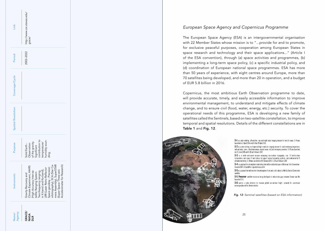
Copernicus, the most ambitious Earth Observation programme to date, will provide accurate, timely, and easily accessible information to improve environmental management, to understand and mitigate effects of climate change, and to ensure civil (food, water, energy, etc.) security. To cover the operational needs of this programme, ESA is developing a new family of satellites called the Sentinels, based on two-satellite constellation, to improve temporal and spatial resolutions. Details of the different constellations are in Table 1 and Fig. 12.
Fig. 12: Sentinel satellites (based on ESA information)
2726
MEASURING EVAPOTRANSPIRATION
Water use in an ecosystem is determined by the vegetation transpiration (liquid water vaporisation from tissue to the atmosphere) and the evaporation from soil or water masses (water changed from liquid to vapour between the surface and the atmosphere). In practice, it is difficult to distinguish between the amount of water evaporated directly from bare soil and the amount transpired by vegetation in land surface areas, as both processes are affected by the structure of the vegetation.
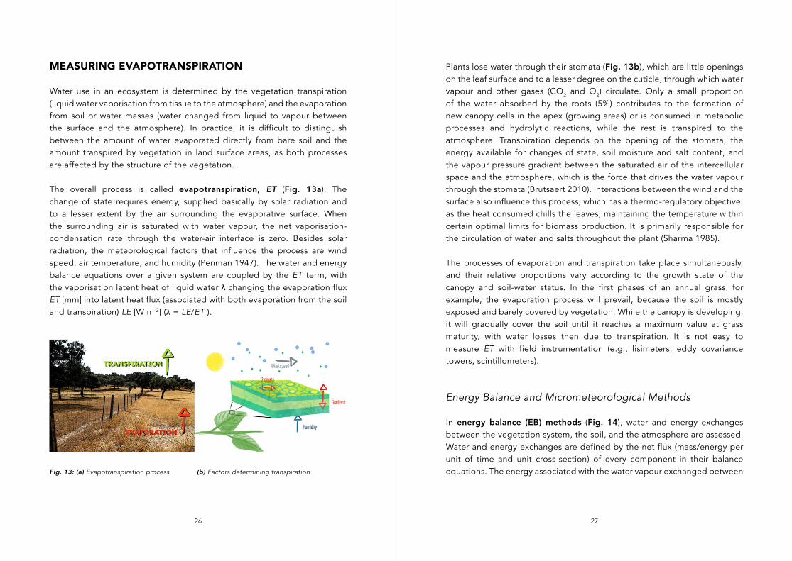
The overall process is called evapotranspiration, ET (Fig. 13a). The change of state requires energy, supplied basically by solar radiation and to a lesser extent by the air surrounding the evaporative surface. When the surrounding air is saturated with water vapour, the net vaporisation-condensation rate through the water-air interface is zero. Besides solar radiation, the meteorological factors that influence the process are wind speed, air temperature, and humidity (Penman 1947). The water and energy balance equations over a given system are coupled by the ET term, with the vaporisation latent heat of liquid water λ changing the evaporation flux ET [mm] into latent heat flux (associated with both evaporation from the soil and transpiration) LE [W m-2] (λ = LE/ET ).
Fig. 13: (a) Evapotranspiration process (b) Factors determining transpiration
Plants lose water through their stomata (Fig. 13b), which are little openings on the leaf surface and to a lesser degree on the cuticle, through which water vapour and other gases (CO2 and O2) circulate. Only a small proportion of the water absorbed by the roots (5%) contributes to the formation of new canopy cells in the apex (growing areas) or is consumed in metabolic processes and hydrolytic reactions, while the rest is transpired to the atmosphere. Transpiration depends on the opening of the stomata, the energy available for changes of state, soil moisture and salt content, and the vapour pressure gradient between the saturated air of the intercellular space and the atmosphere, which is the force that drives the water vapour through the stomata (Brutsaert 2010). Interactions between the wind and the surface also influence this process, which has a thermo-regulatory objective, as the heat consumed chills the leaves, maintaining the temperature within certain optimal limits for biomass production. It is primarily responsible for the circulation of water and salts throughout the plant (Sharma 1985).
The processes of evaporation and transpiration take place simultaneously, and their relative proportions vary according to the growth state of the canopy and soil-water status. In the first phases of an annual grass, for example, the evaporation process will prevail, because the soil is mostly exposed and barely covered by vegetation. While the canopy is developing, it will gradually cover the soil until it reaches a maximum value at grass maturity, with water losses then due to transpiration. It is not easy to measure ET with field instrumentation (e.g., lisimeters, eddy covariance towers, scintillometers).
Energy Balance and Micrometeorological Methods
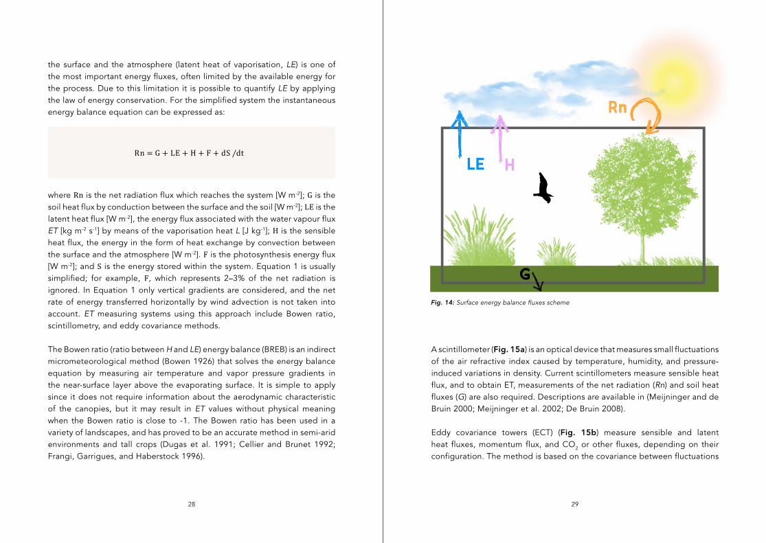
In energy balance (EB) methods (Fig. 14), water and energy exchanges between the vegetation system, the soil, and the atmosphere are assessed. Water and energy exchanges are defined by the net flux (mass/energy per unit of time and unit cross-section) of every component in their balance equations. The energy associated with the water vapour exchanged between
2928
the surface and the atmosphere (latent heat of vaporisation, LE) is one of the most important energy fluxes, often limited by the available energy for the process. Due to this limitation it is possible to quantify LE by applying the law of energy conservation. For the simplified system the instantaneous energy balance equation can be expressed as:
where Rn is the net radiation flux which reaches the system [W m-2]; G is the soil heat flux by conduction between the surface and the soil [W m-2]; LE is the latent heat flux [W m-2], the energy flux associated with the water vapour flux ET [kg m-2 s-1] by means of the vaporisation heat L [J kg-1]; H is the sensible heat flux, the energy in the form of heat exchange by convection between the surface and the atmosphere [W m-2]. F is the photosynthesis energy flux [W m-2]; and S is the energy stored within the system. Equation 1 is usually simplified; for example, F, which represents 2–3% of the net radiation is ignored. In Equation 1 only vertical gradients are considered, and the net rate of energy transferred horizontally by wind advection is not taken into account. ET measuring systems using this approach include Bowen ratio, scintillometry, and eddy covariance methods.
The Bowen ratio (ratio between H and LE) energy balance (BREB) is an indirect micrometeorological method (Bowen 1926) that solves the energy balance equation by measuring air temperature and vapor pressure gradients in the near-surface layer above the evaporating surface. It is simple to apply since it does not require information about the aerodynamic characteristic of the canopies, but it may result in ET values without physical meaning when the Bowen ratio is close to -1. The Bowen ratio has been used in a variety of landscapes, and has proved to be an accurate method in semi-arid environments and tall crops (Dugas et al. 1991; Cellier and Brunet 1992; Frangi, Garrigues, and Haberstock 1996).
Fig. 14: Surface energy balance fluxes scheme
Rn = G + LE + H + F + dS ⁄dt
A scintillometer (Fig. 15a) is an optical device that measures small fluctuations of the air refractive index caused by temperature, humidity, and pressure-induced variations in density. Current scintillometers measure sensible heat flux, and to obtain ET, measurements of the net radiation (Rn) and soil heat fluxes (G) are also required. Descriptions are available in (Meijninger and de Bruin 2000; Meijninger et al. 2002; De Bruin 2008).
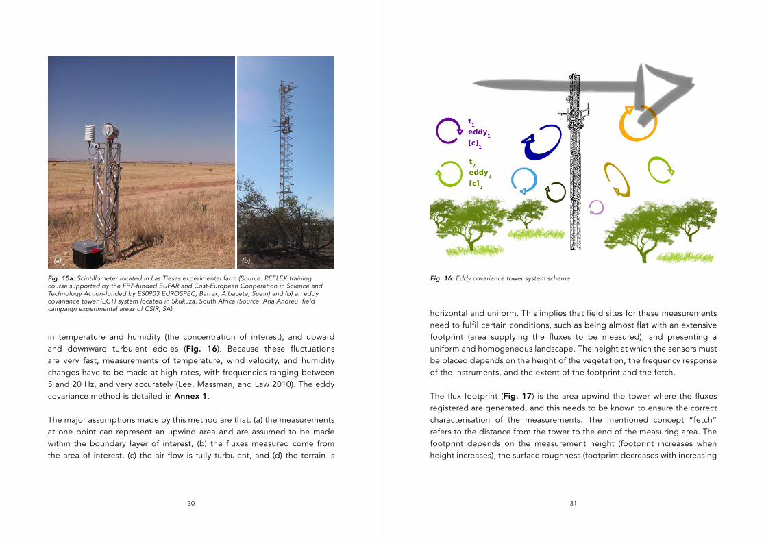
Eddy covariance towers (ECT) (Fig. 15b) measure sensible and latent heat fluxes, momentum flux, and CO2 or other fluxes, depending on their configuration. The method is based on the covariance between fluctuations
3130
in temperature and humidity (the concentration of interest), and upward and downward turbulent eddies (Fig. 16). Because these fluctuations are very fast, measurements of temperature, wind velocity, and humidity changes have to be made at high rates, with frequencies ranging between 5 and 20 Hz, and very accurately (Lee, Massman, and Law 2010). The eddy covariance method is detailed in Annex 1.
The major assumptions made by this method are that: (a) the measurements at one point can represent an upwind area and are assumed to be made within the boundary layer of interest, (b) the fluxes measured come from the area of interest, (c) the air flow is fully turbulent, and (d) the terrain is
Fig. 15a: Scintillometer located in Las Tiesas experimental farm (Source: REFLEX training course supported by the FP7-funded EUFAR and Cost-European Cooperation in Science and Technology Action-funded by ES0903 EUROSPEC, Barrax, Albacete, Spain) and (b) an eddy covariance tower (ECT) system located in Skukuza, South Africa (Source: Ana Andreu, field campaign experimental areas of CSIR, SA)
Fig. 16: Eddy covariance tower system scheme
(a) (b)
horizontal and uniform. This implies that field sites for these measurements need to fulfil certain conditions, such as being almost flat with an extensive footprint (area supplying the fluxes to be measured), and presenting a uniform and homogeneous landscape. The height at which the sensors must be placed depends on the height of the vegetation, the frequency response of the instruments, and the extent of the footprint and the fetch.
The flux footprint (Fig. 17) is the area upwind the tower where the fluxes registered are generated, and this needs to be known to ensure the correct characterisation of the measurements. The mentioned concept “fetch” refers to the distance from the tower to the end of the measuring area. The footprint depends on the measurement height (footprint increases when height increases), the surface roughness (footprint decreases with increasing
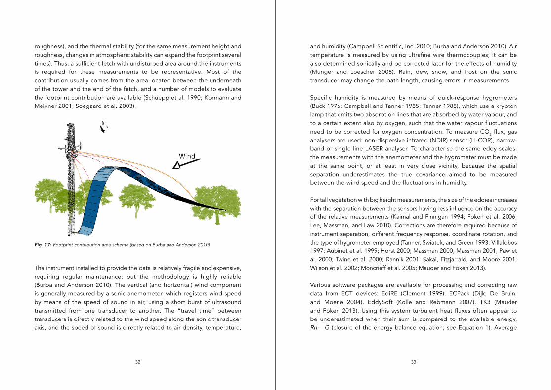
3332
roughness), and the thermal stability (for the same measurement height and roughness, changes in atmospheric stability can expand the footprint several times). Thus, a sufficient fetch with undisturbed area around the instruments is required for these measurements to be representative. Most of the contribution usually comes from the area located between the underneath of the tower and the end of the fetch, and a number of models to evaluate the footprint contribution are available (Schuepp et al. 1990; Kormann and Meixner 2001; Soegaard et al. 2003).
The instrument installed to provide the data is relatively fragile and expensive, requiring regular maintenance; but the methodology is highly reliable (Burba and Anderson 2010). The vertical (and horizontal) wind component is generally measured by a sonic anemometer, which registers wind speed by means of the speed of sound in air, using a short burst of ultrasound transmitted from one transducer to another. The “travel time” between transducers is directly related to the wind speed along the sonic transducer axis, and the speed of sound is directly related to air density, temperature,
Fig. 17: Footprint contribution area scheme (based on Burba and Anderson 2010)
and humidity (Campbell Scientific, Inc. 2010; Burba and Anderson 2010). Air temperature is measured by using ultrafine wire thermocouples; it can be also determined sonically and be corrected later for the effects of humidity (Munger and Loescher 2008). Rain, dew, snow, and frost on the sonic transducer may change the path length, causing errors in measurements.
Specific humidity is measured by means of quick-response hygrometers (Buck 1976; Campbell and Tanner 1985; Tanner 1988), which use a krypton lamp that emits two absorption lines that are absorbed by water vapour, and to a certain extent also by oxygen, such that the water vapour fluctuations need to be corrected for oxygen concentration. To measure CO2 flux, gas analysers are used: non-dispersive infrared (NDIR) sensor (LI-COR), narrow-band or single line LASER-analyser. To characterise the same eddy scales, the measurements with the anemometer and the hygrometer must be made at the same point, or at least in very close vicinity, because the spatial separation underestimates the true covariance aimed to be measured between the wind speed and the fluctuations in humidity.
For tall vegetation with big height measurements, the size of the eddies increases with the separation between the sensors having less influence on the accuracy of the relative measurements (Kaimal and Finnigan 1994; Foken et al. 2006; Lee, Massman, and Law 2010). Corrections are therefore required because of instrument separation, different frequency response, coordinate rotation, and the type of hygrometer employed (Tanner, Swiatek, and Green 1993; Villalobos 1997; Aubinet et al. 1999; Horst 2000; Massman 2000; Massman 2001; Paw et al. 2000; Twine et al. 2000; Rannik 2001; Sakai, Fitzjarrald, and Moore 2001; Wilson et al. 2002; Moncrieff et al. 2005; Mauder and Foken 2013).
Various software packages are available for processing and correcting raw data from ECT devices: EdiRE (Clement 1999), ECPack (Dijk, De Bruin, and Moene 2004), EddySoft (Kolle and Rebmann 2007), TK3 (Mauder and Foken 2013). Using this system turbulent heat fluxes often appear to be underestimated when their sum is compared to the available energy, Rn – G (closure of the energy balance equation; see Equation 1). Average
3534
closure errors are around 20% to 30% (Twine et al. 2000; Wilson et al. 2002; Foken 2008; Franssen et al. 2010). Possible reasons can be found in the influence of the horizontal advection, the storage of heat in canopies, flux divergences, photosynthesis, errors in the measurement of Rn or G, the frequency response of the sensors, measurement errors on turbulent fluxes, and the separation of the instruments.
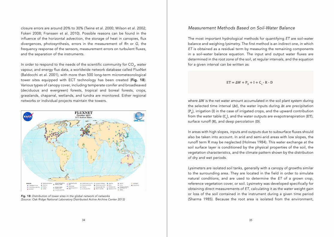
In order to respond to the needs of the scientific community for CO2, water vapour, and energy flux data, a worldwide network database called FluxNet (Baldocchi et al. 2001), with more than 500 long-term micrometeorological tower sites equipped with ECT technology has been created (Fig. 18). Various types of canopy cover, including temperate conifer and broadleaved (deciduous and evergreen) forests, tropical and boreal forests, crops, grasslands, chaparral, wetlands, and tundra are monitored. Either regional networks or individual projects maintain the towers.
Measurement Methods Based on Soil-Water Balance
The most important hydrological methods for quantifying ET are soil-water balance and weighing lysimetry. The first method is an indirect one, in which ET is obtained as a residual term by measuring the remaining components in a soil-water balance equation. The input and output water fluxes are determined in the root zone of the soil, at regular intervals, and the equation for a given interval can be written as:
where ΔW is the net water amount accumulated in the soil plant system during the selected time interval (Δt), the water inputs during Δt are precipitation (PR), irrigation (I) in the case of irrigated crops, and the upward contribution from the water table (Cu), and the water outputs are evapotranspiration (ET), surface runoff (R), and deep percolation (D).
In areas with high slopes, inputs and outputs due to subsurface fluxes should also be taken into account. In arid and semi-arid areas with low slopes, the runoff term R may be neglected (Holmes 1984). This water exchange at the soil surface layer is conditioned by the physical properties of the soil, the vegetation characteristics, and the climate pattern shown by the distribution of dry and wet periods.
Lysimeters are isolated soil tanks, generally with a canopy of growths similar to the surrounding area. They are located in the field in order to simulate natural conditions, and are used to determine the ET of a grown crop, reference vegetation cover, or soil. Lysimetry was developed specifically for obtaining direct measurements of ET, calculating it as the water weight gain or loss of the soil contained in the instrument during a given time period (Sharma 1985). Because the root area is isolated from the environment,
Fig. 18: Distribution of tower sites in the global network of networks(Source: Oak Ridge National Laboratory Distributed Active Archive Center 2013)
ET = ∆W + PR + I + Cu - R - D
3736
lateral fluxes, percolation, and capillary rise are null. The rest terms of the balance can be accurately determined. The water loss or gain is given by the mass change over time, obtained by continuously weighing the soil tank. For the lysimeter measures to be representative of whole field conditions, the density of the inside vegetation and the height and soil characteristics need to be similar to the surrounding area (Grebet and Cuenca 1991).
Plant Physiology Approaches
These methods analyse the water behaviour of individual plants based on their physiology. The chamber system (Reicosky and Peters 1977; Wagner and Reicosky 1996) and sap flow method (Cohen et al. 1988) are the most widely used (Rana and Katerji 2000).
The sap flow method is based on the assumption that this flow is related to the canopy transpiration rate. Applications at canopy scale require individual measurements to be extrapolated to the scale of interest, which is possible when the structure of the canopy and the spatial variability (density, height, and leaf area index, LAI) are known. The effect of evaporation from the soil does not influence this measurement and it is not assessed. In Mediterranean climates with low fractional covers, evaporation from soil can be a very important fraction of the ET (up to 20%), which means that an additional measurement system is required in combination with sap flow to estimate total ET.
Chambers for measuring ET were described for the first time by (Reicosky and Peters 1977). These consist of a plastic chamber in which the air is mixed continuously. Vapour density is measured with infrared analysers and CO2 flux can be also evaluated. The chambers are suitable for research studies on orchard crops such as vines and olive trees (Katerji et al. 1994; Pérez-Priego et al. 2014).
HOW TO ACCOUNT FOR ECOSYSTEM WATER USE USING EARTH OBSERVATION DATA(KC-FAO 56 AND TSEB MODELS)
Due to the difficulties of ground ET measurement, along with the cost, maintenance of instruments, and the non-distributed nature of the data, significant research efforts have been put into estimating ET by using models with different physical foundations. These can be broadly classified into analytical and empirical models (Rana and Katerji 2000). The integration of remotely sensed data into evapotranspiration models has widened its area of application from point to basin and regional scales.
There are basically two research lines devoted to ET estimation using remotely sensed information. The first approach uses the vegetation indexes (VI) derived from airborne or satellite measured surface reflectance to determine crop growth and to estimate the basal crop coefficient (Kcb) (Bausch and Neale 1990). Together with data coming from meteorological stations to compute the reference ET (ET0) that accounts for the atmospheric demand, it can be used to determine the actual ET of the crop (Allen et al. 1998) (Allen et al. 1998). The second approach uses the surface radiometric temperature (TRAD) derived from the thermal bands of remote sensors to estimate ET as latent heat flux, as a residual of the energy balance. e.g., (Moran et al. 1994; Kustas and Norman 1996; Gillies, Kustas, and Humes 1997; Bastiaanssen et al. 1998).
Detailed information about the two methods (used in this study to estimate water use in savannas) is compiled in Annex 2, 3 and 4.

4. TOOLS IN PRACTICE
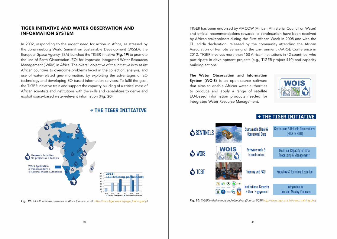
4140
TIGER INITIATIVE AND WATER OBSERVATION AND INFORMATION SYSTEM
In 2002, responding to the urgent need for action in Africa, as stressed by the Johannesburg World Summit on Sustainable Development (WSSD), the European Space Agency (ESA) launched the TIGER initiative (Fig. 19) to promote the use of Earth Observation (EO) for improved Integrated Water Resources Management (IWRM) in Africa. The overall objective of the initiative is to assist African countries to overcome problems faced in the collection, analysis, and use of water-related geo-information, by exploiting the advantages of EO technology and developing EO-based information services. To fulfil the goal, the TIGER initiative train and support the capacity building of a critical mass of African scientists and institutions with the skills and capabilities to derive and exploit space-based water-relevant information (Fig. 20).
Fig. 19: TIGER Initiative presence in Africa (Source: TCBF http://www.tiger.esa.int/page_training.php)
TIGER has been endorsed by AMCOW (African Ministerial Council on Water) and official recommendations towards its continuation have been received by African stakeholders during the First African Week in 2008 and with the El Jadida declaration, released by the community attending the African Association of Remote Sensing of the Environment -AARSE Conference in 2012. TIGER involves more than 150 African institutions in 42 countries, who participate in development projects (e.g., TIGER project 410) and capacity building actions.
The Water Observation and Information System (WOIS) is an open-source software that aims to enable African water authorities to produce and apply a range of satellite EO-based information products needed for Integrated Water Resource Management.
Fig. 20: TIGER Initiative tools and objectives (Source: TCBF http://www.tiger.esa.int/page_training.php)
42
HOW TO
The WOIS is available freely to any interested user pending a short registration. The WOIS was developed within the TIGER initiative as part of the TIGER-NET project in close collaboration with several African transboundary and national water authorities, which provided input on the specifications, tested, and demonstrated the use of the WOIS. Additional information about the WOIS can be found at the following link:http://www.tiger.esa.int/page_eoservices_wois.php
PRODUCT APPLICATIONS
Information about the spatiotemporal distribution of vegetation cover and ET will be aggregated at temporal scales useful for management and planning, providing vital baseline data for the development of sustainable management practices, as well as for evaluating the effect of current practices (e.g., fire, livestock densities, crop production, and grazing) in the ecosystem productivity and maintenance. This information also plays a critical role at the institutional level by assisting to establish areas under water stress where licensing for water use has to be curtailed or protection-conservation actions should be taken.
To continue improving the integration of the Savanna Water Use and Water Stress Tool in rangeland management, your contribution is highly appreciated. Please fill out the online survey about your preferences and suggestions at the following URL: bit.ly/2ov6cDP (questions are as outlined in Annex 5).
4544
PROCESS
Kc-FAO56, integrating reflectance data, is used to derive basal crop coefficient Kcb (with high spatial resolution) and ET0 (from meteorological data, distributed or point measurements), as detailed in Annex 2. Kcb is computed from VI-NDVI, and the evaporation coefficient (Ke) from precipitation data using a reduction coefficient. TSEB, integrating radiometric surface temperature, is used to determine the stress ecosystem evapotranspiration (with low spatial resolution), as detailed in Annex 4. The Ecosystem Stress Index (with low spatial resolution) is derived as the ratio of reference evaporation and actual evaporation. Finally, the Stress Evapotranspiration with high spatial resolution is derived integrating ESI as the water stress index (Ks) in Kc-FAO56.
SYSTEM REQUIREMENTS(NO MINIMUM SYSTEM REQUIREMENTS FOR WOIS)
Computers equipped with Windows or Linux with WINE applicationCPU: Intel Core i5-3570 Processor (Quad Core, 3.4GHz)Memory: 8GB (2x4GB) 1600 MHz ddr3 Non-ECCDisk space
SOFTWARE NEEDED
1. QGIS (free and Open Source Geographic Information System)http://qgis.org
2. WOIS http://www.tiger.esa.int/page_eoservices_wois.php
3. pyTSEB Software from Dr. Nieto and Dr. Guzinski*https://github.com/hectornieto/pyTSEB http://pytseb.readthedocs.io/en/latest/index.html
4. Python and Jupyter Notebook (e.g., Anaconda, which conveniently installs Python, the Jupyter Notebook, and other commonly used packages for scientific computing)https://www.continuum.io/downloads
Additional for Sentinel 2 images:
5. Science Toolbox Exploitation Platform (SNAP/STEP) – Sentinel 2 & 3 Toolbox (requires Anaconda)http://step.esa.int/main/download/
6. Atmospheric correction sen2cor (based in radiative transfer model MODTRAN, which can be run in the graphic interface SNAP or by the terminal)http://s2tbx.telespazio-vega.de/sen2cor
*pyTSEB will be integrated in QGIS and/or WOIS in the near future (item 4 would not be necessary)
DATA NEEDED
1. Earth Observation information• Sentinel 2 multi-spectral image(s) from the area to be analysed (or
SPOT)• Sentinel 3/MODIS radiometric surface temperature from the area to
be analysed
2. Meteorological variables (distributed-matrix or temporal data series)• Air temperature• Wind speed• Relative humidity (vapour pressure)• Incoming shortwave radiation (Sdn)• Precipitation

4746
3. Canopy characteristics• Canopy height (average)• Leaf area index (LAI) and/or vegetation fractional cover (derived from
EO data)
4. Other input variables• Year, Day Of Year (DOY), time (be aware of data consistency)
Results• Vegetation fractional cover – LAI & NDVI• Non-stress vegetation ET with high spatial resolution (10m x 10m)• Stress vegetation ET with low spatial resolution (1km x 1km)• Ecosystem Stress Index with low spatial resolution (1km x 1km)• Stress vegetation ET with high spatial resolution derived from the
integration of the Ecosystem Stress Index (10m x 10m)
DETAILED STEPS
1. Non-stress vegetation ET (SNAP/STEP; WOIS-QGIS) Model framework: Kc-FAO56
1.1 Prepare data with SNAP/STEP to atmospherically correct S2 images• Detailed steps described in:
o http://forum.step.esa.int/c/s2tbx/sen2coro http://step.esa.int/thirdparties/sen2cor/2.3.1/%5BL2A-
SUM%5D%20S2-PDGS-MPC-L2A-SUM%20%5B2.3.0%5D.pdf• Main EO input:
o Sentinel 2 image• Results: Sentinel 2 images reflectance
Command line for atmospheric correction Basic application of the algorithm, just indicate the location where the level L1C is as follows:
L2A_Process-script.py [-h] [--resolution {10,20,60}] [--sc_only] [--profile] directorySentinel-2 Level 2A Prototype Processor (Sen2Cor). Version: 2.0.6, created:2015.12.02, supporting Level-1C product version: 13.positional arguments: directory Directory where the Level-1C input files are locatedoptional arguments: -h, --help show this help message and exit --resolution {10,20,60} Target resolution, must be 10, 20 or 60 [m] --sc_only Performs only the scene classification at 60m resolution --profile Profiles the processor's performance
Graphic interface SNAPOpen SNAP tool and in Tools > Plugins, there is an 'Available Plugins' tab. Locate sen2cor plugin and install it. Restart SNAP. To verify the installation Upper toolbar > Optical> Thematic Land Processing tab > sen2cor tab. Launch the graphical interface of sen2cor. Select in 'processing parameters' tab the value 10 (it is the pixel size in the output image). Indicate output path (as defect, same path as the input image). Press Run (if the path is too long it may fail). The process on a computer with an i7 processor, 4 GB RAM, and SSD disk takes about 30 minutes. The output images are surface reflectances. It is recommended to check the spectral signatures of the different surfaces present in the scene.
1.2 Use of SNAP and/or QGIS and/or WOIS for NDVI, ƒC, LAI calculation• The main input data is an image containing the study area. Any GDAL
compatible raster format should work. The input should include: o Visible band (Band 8 from S2)

4948
o Near infrared band (Band 4 from S2)o Ancillary input: vegetation parameters
• Results: NDVI, fc, and LAI: the algorithm are/will be integrated into WOIS, but you can apply them with:o SNAP > Toolbar menu > Optical > Thematic Land Processing > Vegetation Rad Indices > NDVI Processor. Once NDVI maps are produced, follow: SNAP > Toolbar menu > Raster > Band Maths, and code equations in Annex 3.o QGIS > Toolbar menu > Raster > Raster calculator. Code equations in Annex 3.
1.3 Use of SNAP and/or QGIS and/or WOIS for Non-stress ET• Input data:
o NDVIo Ancillary input: vegetation parameters and ET0-meteorological parameters (Annex 2)
• Results: ET0, Ke, and Kcb surface, generated by applying the algorithms detailed in Annex 2. The algorithms are/will be integrated in WOIS, but you can apply them with:o WOIS – Hydrological Modelling – Reference ETo QGIS > Toolbar menu > Raster > Raster calculator
2. Stress vegetation ET (pyTSEB Software – TSEB-PT)
• Detailed steps described in:o http://pytseb.readthedocs.io/en/latest/README_Notebooks.html
• Main EO input: o Sentinel 3 (MODIS) image containing the radiometric temperature (any GDAL compatible raster format) [degree Celsius]
• Model framework: TSEB-PT• Ancillary input:
o Effective Leaf Area Index [m2/m2] (from Step 1) and/or vegetation fractional cover
o View Zenith Angle [degrees] (from the image metadata)o Canopy height [m]o Canopy width-to-height ratio [w/hc] (optional)o Vegetation green fraction, ƒg (optional)o Air temperature [Celsius]o Wind speed [m/s]o �a: vapour pressure [mb]o Sdn: Incoming shortwave irradiance [W/m2]
• Results: Stress Ecosystem Evapotranspiration with low spatial resolution
Install pyTSEB. › Open your terminal/command line window. › Type 'jupyter notebook'. › Access Jupyter notebook in your browser. › Look for .ipynb file from pyTSEB in your computer folder. › Follow detailed steps described in pyTSEB by Hector Nieto.
3. Stress index (SNAP-WOIS-QGIS) andStress Evapotranspiration at high resolution
• EO data: Results from Step 1 (ET0, Ke, and Kc) and Step 3 (ET).• Model framework: Ratio between non-stress ET and stress ET• Results: Ecosystem Stress Index (ESI) with low spatial resolution and
Stress ET with high spatial resolutionAlgorithms will be integrated in WOIS, but you can apply them in your area with:• SNAP > Raster > Band Maths• QGIS > Toolbar menu > Raster > Raster calculator
ESI = (ET0 (Step 1.3)/ET (Step 2))Kc = Ke (Step 1.3) + Kcb (Step 1.3) ESI (of the area – Step 2)Stress ET at high resolution = KcET0

REFERENCES
5352
Alcaraz-Segura, D. 2014. Earth Observation of Ecosystem Services. Boca Raton, FL: CRC Press.
Allen, R. G., L. Pereira, D. Raes, and M. Smith. 1998. Crop Evapotranspiration, Guidelines for
Computing Crop Water Requirements. Rome. http://www.fao.org/docrep/X0490E/x0490e00.htm.
Andreu, A. 2014. “Water monitoring in vegetation covers through multi-scale energy balance
modelling using time series of remotely sensed data.” PhD diss., University of Córdoba.
http://hdl.handle.net/10396/12478.
Andreu, A., M. P. González-Dugo, W. P. Kustas, M. J. Polo, and M. C. Anderson. 2013. “Modelling
Surface Energy Fluxes over a Dehesa Ecosystem Using a Two-Source Energy Balance Model and
Medium Resolution Satellite Data.” In , 8887:888717-888717–15. doi:10.1117/12.2029235.
Asner, G. P., S. R. Levick, and Kennedy-Bowdoin. 2009. “Large-Scale Impacts of Herbivores on the
Structural Diversity of African Savannas.” In Proceedings of the National Academy of Sciences.
Asner, G.P., and S. R. Levick. 2012. “Landscape-Scale Effects of Herbivores on Treefall in African
Savannas.” Ecology Letters 15 (11): 1211–17. doi:10.1111/j.1461-0248.2012.01842.x.
Asner, G.P., N. Vaughn, I.P.J Smit, and S. Levick. 2016. “Ecosystem-Scale Effects of Megafauna in
African Savannas.” Ecography 39 (2): 240–52. doi:10.1111/ecog.01640.
Asner, N. Owen-Smith, S. R. Loarie, A. B. Davies, E. Le Roux, and S. R. Levick. 2015. “Habitat
Differences Do Not Explain Population Declines of Sable Antelope in an African Savanna.” Journal of
Zoology 297 (3): 225–34. doi:10.1111/jzo.12269.
Asrar, G., E.T. Kanemasu, and M. Yoshida. 1985. “Estimates of Leaf Area Index from Spectral Reflectance
of Wheat under Different Cultural Practices and Solar Angle.” Remote Sensing of Environment 17 (1):
1–11. doi:10.1016/0034-4257(85)90108-7.
Aubinet, M., A. Grelle, A. Ibrom, Ü. Rannik, J. Moncrieff, T. Foken, A. S. Kowalski, et al. 1999.
“Estimates of the Annual Net Carbon and Water Exchange of Forests: The EUROFLUX Methodology.”
In Advances in Ecological Research, edited by A. H. Fitter and D. G. Raffaelli, 30:113–75. Academic
Press. http://www.sciencedirect.com/science/article/pii/S0065250408600185.
Baldocchi, D.D., E. Falge, L. Gu, R. Olson, D. Hollinger, S. Running, P. Anthoni, et al. 2001. “FLUXNET:
A New Tool to Study the Temporal and Spatial Variability of Ecosystem–Scale Carbon Dioxide, Water
Vapor, and Energy Flux Densities.” Bulletin of the American Meteorological Society 82 (11): 2415–34.
doi:10.1175/1520-0477(2001)082<2415:FANTTS>2.3.CO;2.
Baldocchi, D.D., and L. Xu. 2007. “What Limits Evaporation from Mediterranean Oak Woodlands – The
Supply of Moisture in the Soil, Physiological Control by Plants or the Demand by the Atmosphere?”
Recent Developments in Hydrologic Analysis 30 (10): 2113–22. doi:10.1016/j.advwatres.2006.06.013.
Bastiaanssen, W.G.M., M. Menenti, R.A. Feddes, and A.A.M. Holtslag. 1998. “A Remote Sensing
Surface Energy Balance Algorithm for Land (SEBAL). 1. Formulation.” Journal of Hydrology 212–213
(December): 198–212. doi:10.1016/S0022-1694(98)00253-4.
Bausch, W. C., and C. M. U. Neale. 1990. “Spectral Inputs Improve Corn Crop Coefficients and
Irrigation Scheduling.” Transactions of the ASAE 32 (6): 1901–8. doi:10.13031/2013.31241.
Beerling, D.J., and C.P. Osborne. 2006. “The Origin of the Savanna Biome.” Global Change Biology
12 (11): 2023–31. doi:10.1111/j.1365-2486.2006.01239.x.
Bond, W.J., and J.E. Keeley. 2005. “Fire as a Global ‘herbivore’: The Ecology and Evolution of
Flammable Ecosystems.” Trends in Ecology & Evolution 20 (7): 387–94. doi:10.1016/j.tree.2005.04.025.
Bond, W.J., J.A. Silander Jr, J. Ranaivonasy, and J. Ratsirarson. 2008. “The Antiquity of Madagascar’s
Grasslands and the Rise of C4 Grassy Biomes.” Journal of Biogeography 35 (10): 1743–58.
doi:10.1111/j.1365-2699.2008.01923.x.
Bowen, I. S. 1926. “The Ratio of Heat Losses by Conduction and by Evaporation from Any Water
Surface.” Physical Review 27 (6): 779–87.
Brutsaert, W. 2010. Evaporation into the Atmosphere: Theory, History and Applications. Dordrecht,
The Netherlands: Kluwer.
5554
Buck, A.L. 1976. “The Variable-Path Lyman-Alpha Hygrometer and Its Operating Characteristics.”
Bulletin of the American Meteorological Society 57 (9): 1113–18. doi:10.1175/1520-
0477(1976)057<1113:TVPLAH>2.0.CO;2.
Burba, G., and D. Anderson. 2010. A Brief Practical Guide to Eddy Covariance Flux Measurements:
Principles and Workflow Examples for Scientific and Industrial Applications. Lincoln, Neb.: LI-COR.
Cammalleri, C., M. C. Anderson, G. Ciraolo, G. D’Urso, W. P. Kustas, G. La Loggia, and M. Minacapilli.
2010. “The Impact of in-Canopy Wind Profile Formulations on Heat Flux Estimation in an Open
Orchard Using the Remote Sensing-Based Two-Source Model.” Hydrol. Earth Syst. Sci. 14 (12): 2643–
59. doi:10.5194/hess-14-2643-2010.
Campbell, G.S., and B.D. Tanner. 1985. “A Krypton Hygrometer for Measurement of Atmospheric
Water Vapor Concentration.”
Campbell Scientific, Inc. 2010. CSAT3 Three Dimensional Sonic Anemometer. Campbell Scientific, Inc.
Logan, Utah, United States.
Campos, I., J. Villodre, A. Carrara, and A. Calera. 2013. “Remote Sensing-Based Soil Water Balance
to Estimate Mediterranean Holm Oak Savanna (Dehesa) Evapotranspiration under Water Stress
Conditions.” Journal of Hydrology 494 (June): 1–9. doi:10.1016/j.jhydrol.2013.04.033.
Casey, K. A., A. Kääb, and D. I. Benn. 2012. “Geochemical Characterization of Supraglacial Debris
via in Situ and Optical Remote Sensing Methods: A Case Study in Khumbu Himalaya, Nepal.” The
Cryosphere 6 (1): 85–100. doi:10.5194/tc-6-85-2012.
Cellier, P., and Y. Brunet. 1992. “Flux-Gradient Relationships above Tall Plant Canopies.” Agricultural
and Forest Meteorology 58 (1): 93–117. doi:10.1016/0168-1923(92)90113-I.
Choudhury, B.J., N.U. Ahmed, S.B. Idso, R.J. Reginato, and C.S.T. Daughtry. 1994. “Relations between
Evaporation Coefficients and Vegetation Indices Studied by Model Simulations.” Remote Sensing of
Environment 50 (1): 1–17. doi:10.1016/0034-4257(94)90090-6.
Chuvieco, E., and A. Huete. 2010. Fundamentals of Satellite Remote Sensing. Boca Raton [u.a.: CRC
Press.
Clement, R. 1999. EdiRe Data Software 1.5.0.10. Edinburgh, England.
Cohen, Y., M. Fuchs, V. Falkenflug, and S. Moreshet. 1988. “Calibrated Heat Pulse Method
for Determining Water Uptake in Cotton.” Agronomy Journal 80 (3): 398–402. doi:10.2134/
agronj1988.00021962008000030004x.
De Bruin, H.A.R. 2008. Theory and Application of Large Aperture Scintillometers. Scintec Corp.
Dijk, A. F., Henk De Bruin, and A. F. Moene. 2004. “The Principles of Surface Flux Physics: Theory,
Practice and Description of the ECPACK Library.” http://edepot.wur.nl/44341.
Dugas, W.A., L.J. Fritschen, L.W. Gay, A.A. Held, A.D. Matthias, D.C. Reicosky, P. Steduto, and J.L.
Steiner. 1991. “Bowen Ratio, Eddy Correlation, and Portable Chamber Measurements of Sensible
and Latent Heat Flux over Irrigated Spring Wheat.” Agricultural and Forest Meteorology 56 (1): 1–20.
doi:10.1016/0168-1923(91)90101-U.
Foken, T. 2008. “The Energy Balance Closure Problem: An Overview.” Ecological Applications 18 (6):
1351–67. doi:10.1890/06-0922.1.
Foken, T., F Wimmer, M. Mauder, C. Thomas, and C. Liebethal. 2006. “Some Aspects of the Energy
Balance Closure Problem.” Atmospheric Chemistry and Physics, European Geosciences Union 6 (12):
4395–4402.
Frangi, J.P., C. Garrigues, and H. Haberstock. 1996. “Evapotranspiration and Stress Indicator through
Bowen Ratio Method.” In Proceedings of the International Conference. San Antonio, Texas: Camp
CR, Yoder RE.
Franssen, H.J. Hendricks, R. Stöckli, I. Lehner, E. Rotenberg, and S.I. Seneviratne. 2010. “Energy
Balance Closure of Eddy-Covariance Data: A Multisite Analysis for European FLUXNET Stations.”
Agricultural and Forest Meteorology 150 (12): 1553–67. doi:10.1016/j.agrformet.2010.08.005.
5756
Gillies, R. R., W. P. Kustas, and K. S. Humes. 1997. “A Verification of the ‘Triangle’ Method for Obtaining
Surface Soil Water Content and Energy Fluxes from Remote Measurements of the Normalized
Difference Vegetation Index (NDVI) and Surface E.” International Journal of Remote Sensing 18 (15):
3145–66. doi:10.1080/014311697217026.
Glenn, E.P., A Huete, P. Nagler, and S.G. Nelson. 2008. “Relationship Between Remotely-Sensed
Vegetation Indices, Canopy Attributes and Plant Physiological Processes: What Vegetation Indices
Can and Cannot Tell Us About the Landscape.” Sensors 8: 2136–60.
Gonzalez-Dugo, M.P., C.M.U. Neale, L. Mateos, W.P. Kustas, J.H. Prueger, M.C. Anderson, and
F. Li. 2009. “A Comparison of Operational Remote Sensing-Based Models for Estimating Crop
Evapotranspiration.” Special Section on Water and Carbon Dynamics in Selected Ecosystems in China
149 (11): 1843–53. doi:10.1016/j.agrformet.2009.06.012.
Gordon, H.R., and A.Y. Morel. 1983. Remote Assessment of Ocean Color for Interpretation of Satellite
Visible Imagery: A Review. New York: Springer.
Grebet, P., and R. H. Cuenca. 1991. “History of Lysimeter Design and Effects of Environmental
Disturbances.” In Proceedings of International Symposium on Lysimetry. ASCE, New York, NY: R. G.
Allen, T. A. Howell, W. O. Pruit, I. A. Walter, & M. E. Jensen.
Hatfield, J. L. 1997. “Plant-Water Interactions.” In Plants for Environmental Studies, 81–103. New York:
C. L. Publishers.
Holmes, J.W. 1984. “Measuring Evapotranspiration by Hydrological Methods.” In Developments
in Agricultural and Managed Forest Ecology, edited by M.L. SHARMA, Volume 13:29–40. Elsevier.
http://www.sciencedirect.com/science/article/pii/B9780444422507500069.
Horst, T. W. 2000. “On Frequency Response Corrections for Eddy Covariance Flux Measurements.”
Boundary-Layer Meteorology 94 (3): 517–20. doi:10.1023/A:1002427517744.
Huete, A, K Didan, T Miura, E.P Rodriguez, X Gao, and L.G Ferreira. 2002. “Overview of the Radiometric
and Biophysical Performance of the MODIS Vegetation Indices.” The Moderate Resolution Imaging
Spectroradiometer (MODIS): A New Generation of Land Surface Monitoring 83 (1–2): 195–213.
doi:10.1016/S0034-4257(02)00096-2.
Huete, A.R. 1988. “A Soil-Adjusted Vegetation Index (SAVI).” Remote Sensing of Environment 25 (3):
295–309. doi:10.1016/0034-4257(88)90106-X.
Idso, S.B., and D.G. Baker. 1967. “Relative Importance of Reradiation, Convection, and Transpiration
in Heat Transfer from Plants.” Plant Physiology 42 (5): 631–40. doi:10.1104/pp.42.5.631.
IPCC. 2014. Climate Change 2014: Synthesis Report. Contribution of Working Groups I, II and III to
the Fifth Assessment Report of the Intergovernmental Panel on Climate Change. Geneva, Switzerland:
Pachauri, R.K., Meyer, L.A.
Jeltsch, F., G.E. Weber, and V. Grimm. 2000. “Ecological Buffering Mechanisms in Savannas:
A Unifying Theory of Long-Term Tree-Grass Coexistence.” Plant Ecology 150 (1): 161–71.
doi:10.1023/A:1026590806682.
Jensen, J.R. 2000. Remote Sensing of the Environment: An Earth Resource Perspective (2nd Edition).
Prentice-Hall.
Kaimal, J. C., and J. J. Finnigan. 1994. “Atmospheric Boundary Layer Flows : Their Structure and
Measurement.” http://public.eblib.com/choice/publicfullrecord.aspx?p=271025.
Kamaljit, K. 2006. “The Role of Ecosystem Services from Tropical Savannas in Well-Being of Aboriginal
People: A Scoing Study.” Tropical Savannas Cooperative Research Centre. School of Business, James
Cook University. Darwin, NT.
Katerji, N., F.A. Daudet, A. Carbonneau, and N. Ollat. 1994. “Photosynthesis and Transpiration Studies
with Traditionally and Lyre-Trained Vines.” Vitis 33: 197–203.
Kaufman, Y.J., and C. Sendra. 1988. “Algorithm for Automatic Atmospheric Corrections to Visible and
near-IR Satellite Imagery.” International Journal of Remote Sensing International Journal of Remote
Sensing 9 (8): 1357–81.
Kolle, O., and C. Rebmann. 2007. “EddySoft. Documentation of a Software Package to Acquire and
Process Eddy Covariance Data.” Technical Report.
5958
Kormann, R., and F.X. Meixner. 2001. “An Analytical Footprint Model For Non-Neutral Stratification.”
Boundary-Layer Meteorology 99 (2): 207–24. doi:10.1023/A:1018991015119.
Kueppers, L.M., M.A. Snyder, L.C. Sloan, E.S. Zavaleta, and B. Fulfrost. 2005. “Modeled Regional
Climate Change and California Endemic Oak Ranges.” Proceedings of the National Academy of
Sciences of the United States of America 102 (45): 16281–86. doi:10.1073/pnas.0501427102.
Kustas, W.P., and J.M. Norman. 1996. “Use of remote sensing for evapotranspiration monitoring over
land surfaces.” Hydrological Sciences Journal, 41: 495 – 516.
Lee, X., W. J. Massman, and B.E. Law. 2010. Handbook of Micrometeorology: A Guide for Surface Flux
Measurement and Analysis.
Lenoble, J. 1993. Atmospheric Radiative Transfer. Hampton, Va., USA: A. Deepak Pub.
Massman, W J. 2001. “Reply to Comment by Rannik on ‘A Simple Method for Estimating Frequency
Response Corrections for Eddy Covariance Systems.’” Agricultural and Forest Meteorology. 107 (3):
247.
Massman, W.J. 2000. “A Simple Method for Estimating Frequency Response Corrections for Eddy
Covariance Systems.” Agricultural and Forest Meteorology 104 (3): 185–98. doi:10.1016/S0168-
1923(00)00164-7.
Mauder, M., and Thomas Foken. 2013. “Documentation and Instruction Manual of the Eddy-Covariance
Software Package TK3.” Documentation, description and user guide. Universitaet Bayreuth, Germany.
Mbatha, K.R., and D. Ward. 2010. “The Effects of Grazing, Fire, Nitrogen and Water Availability on
Nutritional Quality of Grass in Semi-Arid Savanna, South Africa.” Journal of Arid Environments 74 (10):
1294–1301. doi:10.1016/j.jaridenv.2010.06.004.
Meijninger, W. M. L., O. K. Hartogensis, W. Kohsiek, J. C. B. Hoedjes, R. M. Zuurbier, and H. A.
R. De Bruin. 2002. “Determination of Area-Averaged Sensible Heat Fluxes with a Large Aperture
Scintillometer over a Heterogeneous Surface – Flevoland Field Experiment.” Boundary-Layer
Meteorology 105 (1): 37–62. doi:10.1023/A:1019647732027.
Meijninger, W.M.L., and H.A.R. de Bruin. 2000. “The Sensible Heat Fluxes over Irrigated Areas in
Western Turkey Determined with a Large Aperture Scintillometer.” Journal of Hydrology 229 (1–2):
42–49. doi:10.1016/S0022-1694(99)00197-3.
Moncrieff, John, Robert Clement, John Finnigan, and Tilden Meyers. 2005. “Averaging, Detrending,
and Filtering of Eddy Covariance Time Series.” In Handbook of Micrometeorology: A Guide for
Surface Flux Measurement and Analysis, edited by Xuhui Lee, William Massman, and Beverly Law,
7–31. Dordrecht: Springer Netherlands. http://dx.doi.org/10.1007/1-4020-2265-4_2.
Moran, M.S., T.R. Clarke, Y. Inoue, and A. Vidal. 1994. “Estimating Crop Water Deficit Using the
Relation between Surface-Air Temperature and Spectral Vegetation Index.” RSE Remote Sensing of
Environment 49 (3): 246–63.
Moran, S., K. S. Humes, and P. J. Pinter. 1997. “The Scaling Characteristics of Remotely-Sensed
Variables for Sparsely-Vegetated Heterogeneous Landscapes.” Journal of Hydrology Journal of
Hydrology 190 (3–4): 337–62.
Munger, J.W., and H.W. Loescher. 2008. “Ameriflux Guidelines for Making Eddy Covariance Flux
Measurements. Ameriflux.” Documentation, description and user guide. Massachusetts, USA: Harvard
University, Cambridge.
Norman, J.M., W.P. Kustas, and K.S. Humes. 1995. “Source Approach for Estimating Soil and
Vegetation Energy Fluxes in Observations of Directional Radiometric Surface Temperature.” Thermal
Remote Sensing of the Energy and Water Balance over Vegetation 77 (3): 263–93. doi:10.1016/0168-
1923(95)02265-Y.
Oak Ridge National Laboratory Distributed Active Archive Center (ORNL DAAC). 2013. FLUXNET
Maps & Graphics Web Page. Available online (http://fluxnet.ornl.gov/maps-graphics) from ORNL
DAAC, Oak Ridge, Tennessee, USA Accessed November 5, 2013
Papanastasis, V. P. 2004. “Vegetation Degradation and Land Use Changes in Agrosilvopastoral
Systems.” In Sustainability of Agrosilvopastoral Systems: Dehesas, Montados, Schnabel, S. & Ferreira,
A., 37:1–12. Advances in Geoecology. Reiskirchen: Catena Verlag.
6160
Paw, K.T., D.D. Baldocchi, T.P. Meyers, and K.B. Wilson. 2000. “Correction Of Eddy-Covariance
Measurements Incorporating Both Advective Effects And Density Fluxes.” Boundary-Layer
Meteorology 97 (3): 487–511. doi:10.1023/A:1002786702909.
Penman, H. L. 1947. Natural Evaporation from Open Water, Bare Soil and Grass. Physics Dept.,
Rothamsted Experimental Station.
Pérez-Priego, O., L. Testi, A.S. Kowalski, F.J. Villalobos, and F. Orgaz. 2014. “Aboveground Respiratory
CO2 Effluxes from Olive Trees (Olea Europaea L.).” Agroforestry Systems 88 (2): 245–55. doi:10.1007/
s10457-014-9672-y.
Rana, G, and N Katerji. 2000. “Measurement and Estimation of Actual Evapotranspiration in the
Field under Mediterranean Climate: A Review.” European Journal of Agronomy 13 (2–3): 125–53.
doi:10.1016/S1161-0301(00)00070-8.
Rannik, Ü. 2001. “A Comment on the Paper by W.J. Massman ‘A Simple Method for Estimating
Frequency Response Corrections for Eddy Covariance Systems.’” Agricultural and Forest Meteorology
107 (3): 241–45. doi:10.1016/S0168-1923(00)00236-7.
Reicosky, D.C., and D.B. Peters. 1977. “A Portable Chamber for Evapotranspiration Measurements
and Irrigation Scheduling.” Agronomy Journal 69 (4): 455–62. doi:10.17660/ActaHortic.1990.278.42.
Richards, J.A., and X. Jia. 2006. Remote sensing digital image analysis: an introduction. Berlin;
Heidelberg; New York: Springer.
Sakai, R.K., D.R. Fitzjarrald, and K.E. Moore. 2001. “Importance of Low-Frequency Contributions to
Eddy Fluxes Observed over Rough Surfaces.” Journal of Applied Meteorology 40 (12): 2178–92.
doi:10.1175/1520-0450(2001)040<2178:IOLFCT>2.0.CO;2.
Sankaran, M., and J. Ratnam. 2013. “African and Asian Savannas A2 - Levin, Simon A.” In Encyclopedia
of Biodiversity (Second Edition), 58–74. Waltham: Academic Press. http://www.sciencedirect.com/
science/article/pii/B9780123847195003555.
Saunders, R. W., and K. T. Kriebel. 1988. “An Improved Method for Detecting Clear Sky and Cloudy
Radiances from AVHRR Data.” International Journal of Remote Sensing International Journal of
Remote Sensing 9 (1): 123–50.
Schnabel, S., R.A. Dahlgren, and G. Moreno. 2013. “Soil and Water Dynamics.” In
Mediterranean Oak Woodland Working Landscapes : Dehesas of Spain and Ranchlands
of California, Campos et al., 91–121. New York: Springer- Verlag. http://link.springer.com/
openurl?genre=book&isbn=978-94-007-6706-5.
Scholes, R. J., and S. R. Archer. 1997. “Tree-Grass Interactions in Savannas.” Annual Review of Ecology
and Systematics 28 (1): 517–44. doi:10.1146/annurev.ecolsys.28.1.517.
Scholes, R. J., and B. H. Walker. 2004. An African Savanna: Synthesis of the Nylsvley Study. Cambridge:
Cambridge University Press.
Schuepp, P. H., M. Y. Leclerc, J. I. MacPherson, and R. L. Desjardins. 1990. “Footprint Prediction of
Scalar Fluxes from Analytical Solutions of the Diffusion Equation.” Boundary-Layer Meteorology 50 (1):
355–73. doi:10.1007/BF00120530.
Sharma, M.L. 1985. “Estimating Evapotranspiration.” In Advances in irrigation. Volume 3., Daniel
Hillel. Orlando: Academic Press.
Sheffield, J., Wood E.F., Chaney N., Guan K., Sadri S., Yuan X., Ogallo L., et al. 2014. “A Drought
Monitoring and Forecasting System for Sub-Sahara African Water Resources and Food Security.” Bull.
Am. Meteorol. Soc. Bulletin of the American Meteorological Society 95 (6): 861–82.
Soegaard, H., N.O. Jensen, E. Boegh, C.B. Hasager, K. Schelde, and A. Thomsen. 2003. “Carbon
Dioxide Exchange over Agricultural Landscape Using Eddy Correlation and Footprint Modelling.”
Agricultural and Forest Meteorology 114 (3–4): 153–73. doi:10.1016/S0168-1923(02)00177-6.
Tanner, B.D. 1988. “Use Requirements for Bowen Ratio and Eddy Correlation Determination O
Evapotranspiration.” In Planning Now for Irrigation and Drainage in the 21st Century. Lincoln,
Nebraska,: Hay Delynn R.
62
ANNEXES
Tanner, B.D., E. Swiatek, and J.P. Green. 1993. “Density Fluctuations and Use of the Krypton
Hygrometer in Surface Flux Measurements.” In Management of Irrigation and Drainage Systems :
Integrated Perspectives : Park City, Utah, July 21-23, 1993, 105–12. Park City, Utah. New York: Allen,
R.G. American Society of Civil Engineers.
Twine, T.E., W.P. Kustas, J.M. Norman, D.R. Cook, P.R. Houser, T.P. Meyers, J.H. Prueger, P.J. Starks, and
M.L. Wesely. 2000. “Correcting Eddy-Covariance Flux Underestimates over a Grassland.” Agricultural
and Forest Meteorology 103 (3): 279–300. doi:10.1016/S0168-1923(00)00123-4.
Villalobos, F.J. 1997. “Correction of Eddy Covariance Water Vapor Flux Using Additional
Measurements of Temperature.” Agricultural and Forest Meteorology 88 (1): 77–83. doi:10.1016/
S0168-1923(97)00046-4.
Wagner, S.W., and D.C. Reicosky. 1996. “Mobile Research Gas Exchange Machine-MRGEM
Instrumentation Update.” In Proceedings of the International Conference. San Antonio, Texas: Camp
CR, Yoder RE.
Wilgen, B.W. van. 2010. “The Evolution of Fire Management Practices in Savanna Protected Areas in
South Africa.” http://www.sajs.co.za/index.php/SAJS/article/view/107.
Wilson, K., A. Goldstein, E. Falge, M. Aubinet, D. Baldocchi, P. Berbigier, C. Bernhofer, et al. 2002.
“Energy Balance Closure at FLUXNET Sites.” FLUXNET 2000 Synthesis 113 (1–4): 223–43. doi:10.1016/
S0168-1923(02)00109-0.
Wittich, K-P., and O. Hansing. 1995. “Area-Averaged Vegetative Cover Fraction Estimated from
Satellite Data.” International Journal of Biometeorology 38 (4): 209–15. doi:10.1007/BF01245391.
Alcaraz-Segura, Domingo. 2014. Earth Observation of Ecosystem Services. Boca Raton, FL: CRC Press.
6564
EDDY COVARIANCE METHOD
In a turbulent air flow, assuming that air density fluctuations and the mean vertical flow are negligible, the associated energy fluxes can be represented as the product of the mean air density (ρa) and the mean covariance between the instantaneous fluctuations (differences between the instantaneous value and the average value over a given time period) of the vertical wind speed (w’) and a state variable (s’):
The latent heat flux, LE, is computed from the covariance between w’ and the instantaneous fluctuations of the specific air humidity (q’).
By analogy, the sensible heat flux, H, is computed from the covariance between w’ and the instantaneous fluctuations of the air temperature (T’), following the equation:
where Cp is the specific heat for air at constant pressure.
CROP COEFFICIENT METHOD(WHEN ET IS COMPUTED WITH VEGETATION INDEXES)
The basal crop coefficient Kcb obtained from multispectral imagery will be related to the ratio of non-stress canopy ET to reference ET (FAO-56 method). This provides robust and continuous estimation of the ET in an unstressed status (Fig. 21). Due to the high spatial resolution of the VIS/NIR information (10 metres), this approach provides the resolution required for farm/local scales. The inputs to compute ET0 are: the slope of saturation vapour pressure versus average temperature (Δ [kPa °C-1]), net radiation (Rn [mm Δt-1]) and soil heat flux (G [mm Δt-1]), the actual and saturation vapour pressure (ea and es [kPa]), the average temperature (T [°C]), wind velocity (u2 [m s-1]), and the resistance coefficients.
REFERENCECampos, I., J. Villodre, A. Carrara, and A. Calera. 2013. “Remote Sensing-Based Soil Water
Balance to Estimate Mediterranean Holm Oak Savanna (Dehesa) Evapotranspiration under Water
Stress Conditions.” Journal of Hydrology 494 (June): 1–9. doi:10.1016/j.jhydrol.2013.04.033.
ANNEX I ANNEX II
F≈ ρa w’s’
H = ρaCp w’T’
Lρa w’q’
Fig. 21: ET0 and crop coefficient method
*Campos et al. 2013
(A1.3)
(A1.2)
(A1.1)
6766
NORMALISED DIFFERENCE VEGETATION INDEX (NDVI)
NIR (band 8 of Sentinel 2) and Red (band 4 of Sentinel 2) bands are used to retrieve Normalised Difference Vegetation Index (NDVI), following the basic equation:
The scaled NDVI approach (Choudhury et al. 1994) method is used to retrieve ƒc(0) with NDVI remote data:
where NDVIMAX and NDVIMIN represent a surface fully covered by vegetation (~0.9) and completely bare (~0.08), respectively. The parameter p represents the ratio of a leaf angle distribution term (k) to canopy extinction (k'), where p=k/k'. k is the leaf angle distribution function, which appears to range between 0.5–0.7 (Ross 1975) depending on the leaves being distributed randomly (k = 0.5), vertically (k < 0.5), or horizontally (k > 0.5). We believe that it is possible to assume a random distribution because the savanna ecosystem contains erectophile grasses and planophile oak trees. k' is the damping coefficient, ranging between 0.8 and 1.3 for the NDVI (Baret and Guyot 1991; Delegido et al. 2011). We used a weighted p parameter of ~0.9, with k ~0.5 and k' ~ 0.55.
ANNEX III
Leaf area index is derived from fractional cover by an exponential function as Choudhury (1987) suggested:
Because the model was originally developed for uniformly distributed crops, in the case of clumped canopies with partial vegetation cover such as savannas, the parameterisations have to be corrected by a clumping factor (Campbell and Norman 2009; Kustas and Norman 2000) in order to take the particular distribution of the vegetation into account. This factor corrects for the reduction in the extinction of the radiation in a clumped canopy as compared to a uniformly distributed one by multiplying the LAI by a clumping factor (e.g., calculation of clumping factor based on Kustas and Norman (2000)).
In the Santa Clotilde experimental site, the tree-local LAIL measured in the field was 2.6 and the fractional vegetation cover was ƒc = 0.2. So, the ecosystem leaf area index would be LAI = LAIL ƒc ≈ 0.52. If all the leaves were randomly distributed, then the transmission of this vegetated region will be ƒc exp (-0.5LAIL). The fraction of the nadir view occupied by the soil is then ƒc exp (-0.5 LAIL) + (1-ƒc) ≈ 0.854 so that exp (-0.5 Ω LAI) ≈ 0.854 yielding a Ω(0) for the trees of 0.61.
NDVI = NIR – REDNIR + RED
ƒc(0) = 1– � �p
NDVIMAX–NDVI
NDVIMAX–NDVIMIN
(A3.1)
(A3.2)
LAI = ln � �ln�1–ƒc�
–k(A3.3)
68
REFERENCES
Baret, F., and G. Guyot. 1991. “Potentials and Limits of Vegetation Indices for LAI and APAR
Assessment.” Remote Sensing of Environment 35 (2):161–73. doi:10.1016/0034-4257(91)90009-U.
Campbell, Gaylon S., and John M. Norman. 2009. An Introduction to Environmental Biophysics.
Delhi: Springer.
Campos, Pablo. 2013. Mediterranean Oak Woodland Working Landscapes: Dehesas of Spain and
Ranchlands of California. http://link.springer.com/openurl?genre=book&isbn=978-94-007-6706-5.
Choudhury, B.J. 1987. “Relationships between Vegetation Indices, Radiation Absorption, and Net
Photosynthesis Evaluated by a Sensitivity Analysis.” Remote Sensing of Environment 22 (2):209–
33. doi:10.1016/0034-4257(87)90059-9.
Choudhury, B.J., N.U. Ahmed, S.B. Idso, R.J. Reginato, and C.S.T. Daughtry. 1994. “Relations
between Evaporation Coefficients and Vegetation Indices Studied by Model Simulations.” Remote
Sensing of Environment 50 (1):1–17. doi:10.1016/0034-4257(94)90090-6.
Delegido, Jesús, Jochem Verrelst, Luis Alonso, and José Moreno. 2011. “Evaluation of Sentinel-2
Red-Edge Bands for Empirical Estimation of Green LAI and Chlorophyll Content.” Sensors (Basel,
Switzerland) 11(7):7063–81. doi:10.3390/s110707063.
Kustas, William P., and John M. Norman. 2000. “A Two-Source Energy Balance Approach Using
Directional Radiometric Temperature Observations for Sparse Canopy Covered Surfaces.”
Agronomy Journal 92 (5): 847–54. doi:10.2134/agronj2000.925847x.
Ross, J. 1975. “Radiative transfer in plant communities.” Vegetation and the Atmosphere 1:13–56.
London, New York, San Francisco: Academic Press.
7170
ENERGY BALANCE, TSEB METHOD(WHEN ET IS COMPUTED AS LE USING SURFACE RADIOMETRIC TEMPERATURE)
The ET estimation approaches based on the energy balance equation require the aerodynamical temperature (T0) to be obtained – the extrapolation of the air temperature profile down to an effective height within the canopy at which the vegetation component of sensible heat flux arises (Kalma and Jupp 1990), which is not equivalent to the TRAD given by the sensor/satellite. Several schemes have been formulated with different degrees of complexity and requirements for input parameters to solve this problem.
For regional estimations, considering the effects of a partial vegetation cover, the two-source EB model used in this study (Norman, Kustas, and Humes 1995; Kustas and Norman 1999) is of great interest; because it separately formulates the flux energy exchange between the atmosphere and the soil, and between the atmosphere and the vegetation. Moreover, it has a stronger physical basis than other models and allows for adaptation to the specific characteristics of each ecosystem, modifying some aspects of the energy balance to account for the particular physiological, phenological, and meteorological conditions.
The model used in this study was the updated version of the Two-Source Energy Balance (TSEB) model as described by (Kustas and Norman 1999) and (Li et al. 2005). The model assumes that the surface radiometric temperature (TRAD) is a combination of soil (TS) and canopy (TC) temperatures, weighted by the vegetation fraction (fC) derived from the sensor.
The surface energy-balance equation can be formulated for the entire soil-canopy-atmosphere system, or for the soil (subfix s) and canopy (subfix c)
ANNEX IV
F≈ ρa w’s’
TR(ϕ) = {fc(ϕ)TC4 + [1–fc(ϕ)]TS
4 }¼
components separately (Fig. 22). Since the radiation formulation follows the “layer-approach” (Lhomme and Chehbouni 1999), a simple summation of the soil and canopy components yields the total flux.
The soil heat flux was estimated as a time-dependent function of the net radiation that reaches the soil, as follows:
where tS is the time in seconds relative to solar noon. A represents the maximum value of the ratio G/RnS, assumed to have a constant value of 0.35 (Choudhury 1987; Kustas and Daughtry 1990; Friedl 1996), C[s] is the peak in time position, supposedly equal to 3,600 following (Cellier, Richard, and Robin 1996), and B[s] is set equal to 74,000 (Cammalleri et al. 2010).
Rn = RnC + RnS
H = HC + HS
LEc + LES
G = Acos[2π (tS+C)⁄B]RnS
Fig. 22: Energy balance scheme of TSEB model and equation
(A4.2)
(A4.3)
(A4.4)
(A4.5)
(A4.1)
7372
Within the series resistance scheme, the sensible heat fluxes Hc, Hs, and H were expressed as:
where TAC [K] is the air temperature in the canopy – air space, Rx [s m-1] is the resistance to heat flow of the vegetation leaf boundary layer, Rs [s m-1] is the resistance to heat flow in the boundary layer above the soil, and RA [s m-1] is the aerodynamic resistance calculated from the stability-corrected temperature profile equations (Brutsaert 2010), using Monin-Obhukov Similarity Theory (MOST).
Finally, the canopy latent heat flux (LEC) was derived, using as initial assumption a potentially transpiring canopy following the Priestley-Taylor equation (Priestley and Taylor 1972):
where αPT is the Priestley-Taylor coefficient, usually taken as 1.26 [-], fg [-] is the green vegetation fraction, Δ [kPa K-1] is the slope of the saturation vapour pressure versus temperature, and γ [kPa K-1] is the psychrometric constant.
If the vegetation is stressed, the Priestley-Taylor approximation, i.e. equation A4.9, overestimates the transpiration of the canopy and negative values of LEs are computed by the model. This unlikely condensation over the soil during daytime indicates the existence of vegetation water stress, and it is solved by an iteration process that reduces αPT until it yields a coefficient value of 0.1, when LEs becomes 0.
REFERENCES
Brutsaert, W. 2010. Evaporation into the Atmosphere: Theory, History and Applications. Dordrecht,
The Netherlands: Kluwer.
Cammalleri, C., M. C. Anderson, G. Ciraolo, G. D’Urso, W. P. Kustas, G. La Loggia, and M.
Minacapilli. 2010. “The Impact of in-Canopy Wind Profile Formulations on Heat Flux Estimation in
an Open Orchard Using the Remote Sensing-Based Two-Source Model.” Hydrol. Earth Syst. Sci.
14 (12): 2643–59. doi:10.5194/hess-14-2643-2010.
Cellier, P., G. Richard, and P. Robin. 1996. “Partition of Sensible Heat Fluxes into Bare Soil
and the Atmosphere.” Agricultural and Forest Meteorology 82 (1): 245–65. doi:10.1016/0168-
1923(95)02328-3.
Choudhury, B.J. 1987. “Relationships between Vegetation Indices, Radiation Absorption, and
Net Photosynthesis Evaluated by a Sensitivity Analysis.” Remote Sensing of Environment 22 (2):
209–33. doi:10.1016/0034-4257(87)90059-9.
Friedl, M. A. 1996. “Relationships among Remotely Sensed Data, Surface Energy Balance, and
Area-Averaged Fluxes over Partially Vegetated Land Surfaces.” Journal of Applied Meteorology
35 (11): 2091–2103. doi:10.1175/1520-0450(1996)035<2091:RARSDS>2.0.CO;2.
Kalma, J.D., and D.L.B. Jupp. 1990. “Estimating Evaporation from Pasture Using Infrared
Thermometry: Evaluation of a One-Layer Resistance Model.” Agricultural and Forest Meteorology
51 (3): 223–46. doi:10.1016/0168-1923(90)90110-R.
Kustas, W.P., and J.M. Norman. 1999. “Evaluation of Soil and Vegetation Heat Flux Predictions
Using a Simple Two-Source Model with Radiometric Temperatures for Partial Canopy Cover.”
Agricultural and Forest Meteorology 94 (1): 13–29. doi:10.1016/S0168-1923(99)00005-2.
Kustas, W.P., and C. S.T Daughtry. 1990. “Estimation of the Soil Heat Flux/net Radiation Ratio
from Spectral Data.” Agricultural and Forest Meteorology 49 (3): 205–23. doi:10.1016/0168-
1923(90)90033-3.
HC = ρaCp (TC – TAC )⁄RX HS = ρaCp (TS – TAC)⁄RS
H = HC + HS = ρaCp (TAC – TA)⁄R A
LEC = αPT fg RnC� � Δ
Δ + γ
(A4.6)
(A4.7)
(A4.8)
(A4.9)
7574
ANNEX V
Lhomme, J.-P, and A Chehbouni. 1999. “Comments on Dual-Source Vegetation–atmosphere
Transfer Models.” Agricultural and Forest Meteorology 94 (3–4): 269–73. doi:10.1016/S0168-
1923(98)00109-9.
Li, F., W. P. Kustas, J. H. Prueger, C. M. U. Neale, and T. J. Jackson. 2005. “Utility of Remote
Sensing–Based Two-Source Energy Balance Model under Low- and High-Vegetation Cover
Conditions.” Journal of Hydrometeorology 6 (6): 878–91. doi:10.1175/JHM464.1.
Norman, J.M., W.P. Kustas, and K.S. Humes. 1995. “Source Approach for Estimating Soil and
Vegetation Energy Fluxes in Observations of Directional Radiometric Surface Temperature.”
Thermal Remote Sensing of the Energy and Water Balance over Vegetation 77 (3): 263–93.
doi:10.1016/0168-1923(95)02265-Y.
Priestley, C. H. B., and R. J. Taylor. 1972. “On the Assessment of Surface Heat Flux and Evaporation
Using Large-Scale Parameters.” Monthly Weather Review 100 (2): 81–92. doi:10.1175/1520-
0493(1972)100<0081:OTAOSH>2.3.CO;2.
SURVEY
Thank you for taking the time to fill this survey to improve our tool, which is going to be used in monitoring savannas ecosystem water use and stress to help to ensure water/food security integrating Earth Observation data. This survey will only take 5 minutes of your time to complete. Be assured that all the information provided is confidential and will just be used to improve the outcomes of the project.
1. Country of origin
_____________________________________________________________________________________________________________________________
2. Which department do you work in and what is your area of specialization?
Department ______________________________________________________________________________________________________
Area of specialization ______________________________________________________________________________________
3. What are the social economic uses of savannas in your country,if some?
Agriculture Tourism Grazing Traditional medicine
Other/explain ______________________________________________________________________________________________
_____________________________________________________________________________________________________________________________

7776
4. What are the major threats facing savannas in your country?
Fire
Climate variability
Overgrazing
Exotic species
Clearance of land for agriculture and human settlement
5. Have you and your department/ministry made use of any tools utilising Earth Observation (EO) data?
Yes
No
If yes please explain some of the tools used:
_______________________________________________________________________________________________________________________
_______________________________________________________________________________________________________________________
6. What is the level of EO data public availability in your country?
_____________________________________________________________________________________________________________________________
_____________________________________________________________________________________________________________________________
_____________________________________________________________________________________________________________________________
7. What are the technological challenges you face in accessing and interpreting EO data?
Lack of reliable internet access to download data
Lack of enough storage capacity for data downloaded
Lack of human resource capacity to process and interpret the data
Other (please explain):
_______________________________________________________________________________________________________________________
_______________________________________________________________________________________________________________________
8. What is the level of the technical knowhow in interpreting the data from EO and using it in monitoring tools in your department?
_____________________________________________________________________________________________________________________________
_____________________________________________________________________________________________________________________________
9. Would there be need for extensive training on the use of the tool and how to interpret the results?
Yes
No
If yes please highlight the areas you would wish covered during training sessions:
_____________________________________________________________________________________________________________________________

78
10. What would be needed to sustain the use of the tool in the long term and have it implemented in your country?
_____________________________________________________________________________________________________________________________
_____________________________________________________________________________________________________________________________
_____________________________________________________________________________________________________________________________
_____________________________________________________________________________________________________________________________
_____________________________________________________________________________________________________________________________
_____________________________________________________________________________________________________________________________
11. Who would be considered as the major stakeholders to make use of the tool and what would be their role in its implementation?
_____________________________________________________________________________________________________________________________
_____________________________________________________________________________________________________________________________
_____________________________________________________________________________________________________________________________
_____________________________________________________________________________________________________________________________
_____________________________________________________________________________________________________________________________
_____________________________________________________________________________________________________________________________
Thank You!

flores.unu.edu
United Nations University Institute for Integrated Management of Material Fluxes and of Resources (UNU-FLORES)
Ammonstrasse 74 01067 Dresden, GermanyTel.: +49 351 8921 9370 | Fax.: +49 351 8921 9389
Email: [email protected]
The United Nations University Institute for Integrated Management of Material Fluxes and of Resources (UNU-FLORES) was established in Dresden, Germany in 2012 with the support of the Federal Ministry of Education and Research (BMBF) and the Ministry for Higher Education, Research and the Arts (SMWK) of the Free State of Saxony, Germany. As part of the United Nations University (UNU), the Institute helps build a bridge between the academic world and the United Nations. UNU encompasses 13 research and training institutes and programmes located in 12 countries around the world. UNU as a whole aims to develop sustainable solutions for pressing global problems of human survival and development.
UNU-FLORES develops strategies to resolve pressing challenges in the area of sustainable use and integrated management of environmental resources such as soil, water and waste. Focusing on the needs of the UN and its member states, particularly developing countries and emerging economies, the Institute engages in research, capacity development, advanced teaching and training as well as dissemination of knowledge. In all activities, UNU-FLORES advances a nexus approach to the sustainable management of environmental resources.
Find more information under: flores.unu.edu
ADVANCING A NEXUS APPROACH TO THE SUSTAINABLEMANAGEMENT OF ENVIRONMENTAL RESOURCES