TIA MLC Formula Sheet

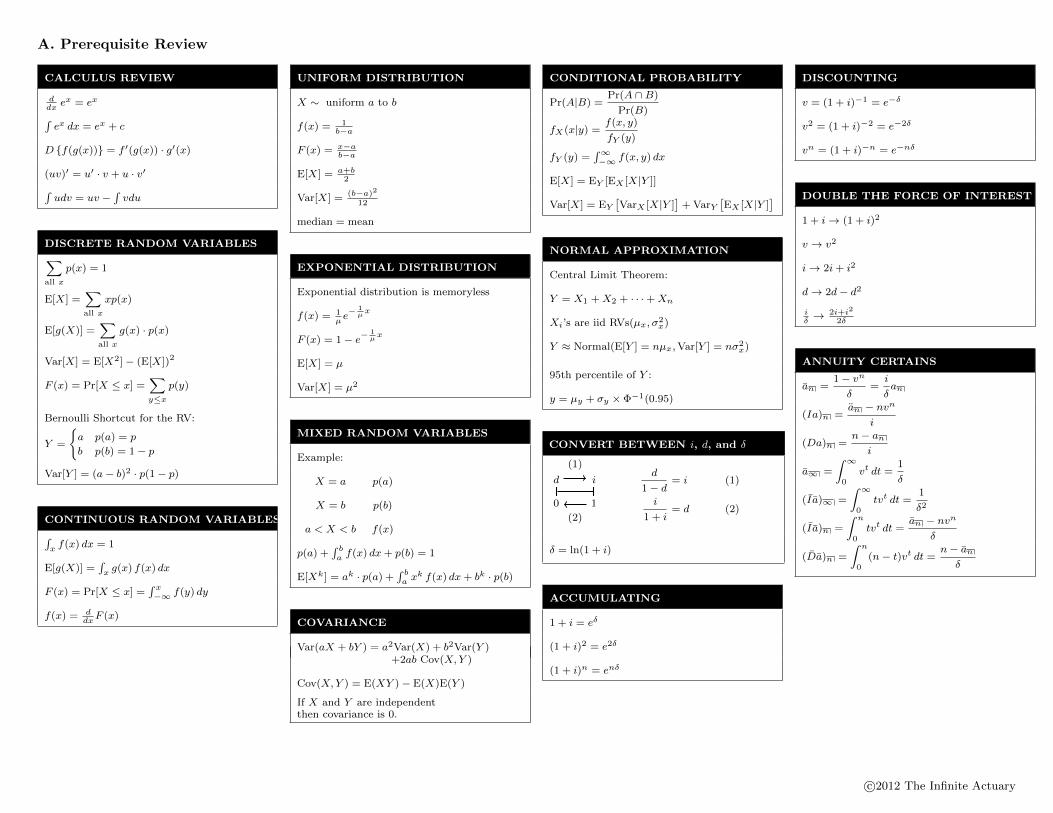
A. Prerequisite Review

CALCULUS REVIEW

ddxex = ex∫ex dx = ex + c

D {f(g(x))} = f ′(g(x)) · g′(x)

(uv)′ = u′ · v + u · v′∫udv = uv −

∫vdu

DISCRETE RANDOM VARIABLES∑all x

p(x) = 1

E[X] =∑all x

xp(x)

E[g(X)] =∑all x

g(x) · p(x)

Var[X] = E[X2]− (E[X])2

F (x) = Pr[X ≤ x] =∑y≤x

p(y)

Bernoulli Shortcut for the RV:

Y =

{a p(a) = p

b p(b) = 1− p

Var[Y ] = (a− b)2 · p(1− p)

CONTINUOUS RANDOM VARIABLES∫x f(x) dx = 1

E[g(X)] =∫x g(x) f(x) dx

F (x) = Pr[X ≤ x] =∫ x−∞ f(y) dy

f(x) = ddxF (x)

UNIFORM DISTRIBUTION

X ∼ uniform a to b

f(x) = 1b−a

F (x) = x−ab−a

E[X] = a+b2

Var[X] =(b−a)2

12

median = mean

EXPONENTIAL DISTRIBUTION

Exponential distribution is memoryless

f(x) = 1µe− 1

µx

F (x) = 1− e−1µx

E[X] = µ

Var[X] = µ2

MIXED RANDOM VARIABLES

Example:

X = a p(a)

X = b p(b)

a < X < b f(x)

p(a) +∫ ba f(x) dx+ p(b) = 1

E[Xk] = ak · p(a) +∫ ba x

k f(x) dx+ bk · p(b)

COVARIANCE

Var(aX + bY ) = a2Var(X) + b2Var(Y )+2ab Cov(X,Y )

Cov(X,Y ) = E(XY )− E(X)E(Y )

If X and Y are independentthen covariance is 0.

CONDITIONAL PROBABILITY

Pr(A|B) =Pr(A ∩B)

Pr(B)

fX(x|y) =f(x, y)

fY (y)

fY (y) =∫∞−∞ f(x, y) dx

E[X] = EY [EX [X|Y ]]

Var[X] = EY[VarX [X|Y ]

]+ VarY

[EX [X|Y ]

]

NORMAL APPROXIMATION

Central Limit Theorem:

Y = X1 +X2 + · · ·+Xn

Xi’s are iid RVs(µx, σ2x)

Y ≈ Normal(E[Y ] = nµx,Var[Y ] = nσ2x)

95th percentile of Y :

y = µy + σy × Φ−1(0.95)

CONVERT BETWEEN i, d, and δ

0

d

1

i

(1)

(2)

d

1− d= i (1)

i

1 + i= d (2)

δ = ln(1 + i)

ACCUMULATING

1 + i = eδ

(1 + i)2 = e2δ

(1 + i)n = enδ

DISCOUNTING

v = (1 + i)−1 = e−δ

v2 = (1 + i)−2 = e−2δ

vn = (1 + i)−n = e−nδ

DOUBLE THE FORCE OF INTEREST

1 + i→ (1 + i)2

v → v2

i→ 2i+ i2

d→ 2d− d2

iδ→ 2i+i2

2δ

ANNUITY CERTAINS

an =1− vn

δ=i

δan

(Ia)n =an − nvn

i

(Da)n =n− an

i

a∞ =

∫ ∞0

vt dt =1

δ

(I a)∞ =

∫ ∞0

tvt dt =1

δ2

(I a)n =

∫ n

0tvt dt =

an − nvn

δ

(Da)n =

∫ n

0(n− t)vt dt =

n− anδ

c©2012 The Infinite Actuary

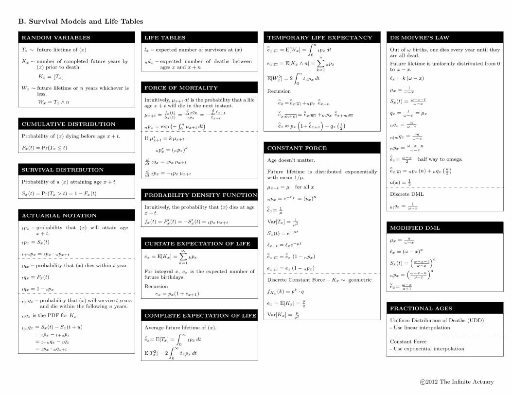
B. Survival Models and Life Tables

RANDOM VARIABLES

Tx ∼ future lifetime of (x)

Kx ∼ number of completed future years by(x) prior to death.

Kx = bTxc

Wx ∼ future lifetime or n years whichever isless.

Wx = Tx ∧ n

CUMULATIVE DISTRIBUTION

Probability of (x) dying before age x+ t.

Fx(t) = Pr(Tx ≤ t)

SURVIVAL DISTRIBUTION

Probability of a (x) attaining age x+ t.

Sx(t) = Pr(Tx > t) = 1− Fx(t)

ACTUARIAL NOTATION

tpx − probability that (x) will attain agex+ t.

tpx = Sx(t)

t+upx = tpx · upx+t

tqx − probability that (x) dies within t year

tqx = Fx(t)

tqx = 1− tpx

t|uqx − probability that (x) will survive t yearsand die within the following u years.

t|qx is the PDF for Kx

t|uqx = Sx(t)− Sx(t+ u)

= tpx − t+upx

= t+uqx − tqx

= tpx · uqx+t

LIFE TABLES

lx − expected number of survivors at (x)

ndx − expected number of deaths betweenages x and x+ n

FORCE OF MORTALITY

Intuitively, µx+t dt is the probability that a lifeage x+ t will die in the next instant.

µx+t =fx(t)Sx(t)

=ddt tqx

tpx=− d

dt`x+t

`x+t

npx = exp(−∫ n0 µx+t dt

)If µ∗x+t = k µx+t :

np∗x = (npx)k

ddt t

qx = tpx µx+t

ddt t

px = −tpx µx+t

PROBABILITY DENSITY FUNCTION

Intuitively, the probability that (x) dies at agex+ t.

fx(t) = F ′x(t) = −S′x(t) = tpx µx+t

CURTATE EXPECTATION OF LIFE

ex = E[Kx] =∞∑k=1

kpx

For integral x, ex is the expected number offuture birthdays.

Recursion

ex = px(1 + ex+1)

COMPLETE EXPECTATION OF LIFE

Average future lifetime of (x).

◦ex= E[Tx] =

∫ ∞0

tpx dt

E[T 2x ] = 2

∫ ∞0

t tpx dt

TEMPORARY LIFE EXPECTANCY

◦ex:n = E[Wx] =

∫ n

0tpx dt

ex:n = E[Kx ∧ n] =n∑k=1

kpx

E[W 2x ] = 2

∫ n

0t tpx dt

Recursion

◦ex=

◦ex:n +npx

◦ex+n

◦ex:m+n =

◦ex:m +mpx

◦ex+m:n

◦ex≈ px

(1+◦ex+1

)+ qx

(12

)

CONSTANT FORCE

Age doesn’t matter.

Future lifetime is distributed exponentiallywith mean 1/µ.

µx+t = µ for all x

npx = e−nµ = (px)n

◦ex=

1µ

Var[Tx] =1µ2

Sx(t) = e−µt

`x+t = `xe−µt

◦ex:n =

◦ex (1− npx)

ex:n = ex (1− npx)

Discrete Constant Force−Kx ∼ geometric

fKx (k) = pk · q

ex = E[Kx] =pq

Var[Kx] =pq2

DE MOIVRE’S LAW

Out of ω births, one dies every year until theyare all dead.

Future lifetime is uniformly distributed from 0to ω − x.`x = k (ω − x)

µx = 1ω−x

Sx(t) =ω−x−tω−x

qx = 1ω−x = µx

nqx = nω−x

n|mqx = mω−x

npx = ω−x−nω−x

◦ex=

ω−x2

half way to omega

◦ex:n = npx (n) + nqx

(n2

)a(x) = 1

2

Discrete DML

k|qx = 1ω−x

MODIFIED DML

µx = aω−x

`x = (ω − x)a

Sx(t) =(ω−x−tω−x

)anpx =

(ω−x−nω−x

)a◦ex=

ω−xa+1

FRACTIONAL AGES

Uniform Distribution of Deaths (UDD)

- Use linear interpolation.

Constant Force

- Use exponential interpolation.


SELECT MORTALITY

[age] = age selected

Read across and then down the table.

GOMPERTZ LAW

µx = Bcx c > 1, B > 0

tpx = exp[−(Bln c

)cx(ct − 1)

]

MAKEHAM LAW

µx = A+Bcx c > 1, B > 0, A ≥ −B

tpx = exp(−At) · exp[−(Bln c

)cx(ct − 1)

]


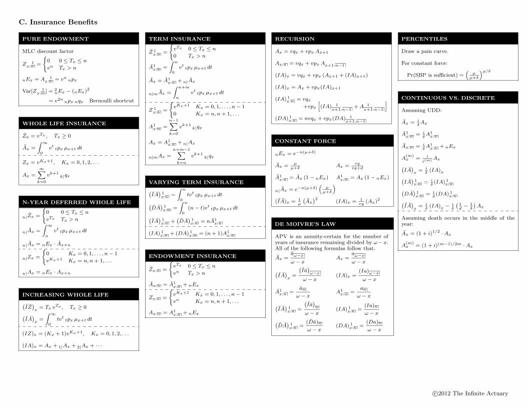
C. Insurance Benefits

PURE ENDOWMENT

MLC discount factor

Z 1x:n =

{0 0 ≤ Tx ≤ n

vn Tx > n

nEx = A 1x:n = vn npx

Var[Z 1x:n ] = 2

nEx − (nEx)2

= v2n npx nqx Bernoulli shortcut

WHOLE LIFE INSURANCE

Zx = vTx , Tx ≥ 0

Ax =

∫ ∞0

vt tpx µx+t dt

Zx = vKx+1, Kx = 0, 1, 2, . . .

Ax =

∞∑k=0

vk+1k|qx

N-YEAR DEFERRED WHOLE LIFE

n|Zx =

{0 0 ≤ Tx ≤ n

vTx Tx > n

n|Ax =

∫ ∞n

vt tpx µx+t dt

n|Ax = nEx · Ax+n

n|Zx =

{0 Kx = 0, 1, . . . , n− 1

vKx+1 Kx = n, n+ 1, . . .

n|Ax = nEx ·Ax+n

INCREASING WHOLE LIFE(IZ)x

= Tx vTx , Tx ≥ 0(IA)x

=

∫ ∞0

tvt tpx µx+t dt

(IZ)x = (Kx + 1)vKx+1, Kx = 0, 1, 2, . . .

(IA)x = Ax + 1|Ax + 2|Ax + · · ·

TERM INSURANCE

Z 1x:n =

{vTx 0 ≤ Tx ≤ n

0 Tx > n

A1x:n =

∫ n

0vt tpx µx+t dt

Ax = A1x:n + n|Ax

n|mAx =

∫ n+m

nvt tpx µx+t dt

Z 1x:n =

{vKx+1 Kx = 0, 1, . . . , n− 1

0 Kx = n, n+ 1, . . .

A1x:n =

n−1∑k=0

vk+1k|qx

Ax = A1x:n + n|Ax

n|mAx =

n+m−1∑k=n

vk+1k|qx

VARYING TERM INSURANCE(IA)1x:n =

∫ n

0tvt tpx µx+t dt(

DA)1x:n =

∫ n

0(n− t)vt tpx µx+t dt(

IA)1x:n +

(DA

)1x:n = nA1

x:n

(IA) 1x:n + (DA) 1

x:n = (n+ 1)A1x:n

ENDOWMENT INSURANCE

Zx:n =

{vTx 0 ≤ Tx ≤ n

vn Tx > n

Ax:n = A1x:n + nEx

Zx:n =

{vKx+1 Kx = 0, 1, . . . , n− 1

vn Kx = n, n+ 1, . . .

Ax:n = A1x:n + nEx

RECURSION

Ax = vqx + vpx Ax+1

Ax:n = vqx + vpx Ax+1:n−1

(IA)x = vqx + vpx (Ax+1 + (IA)x+1)

(IA)x = Ax + vpx(IA)x+1

(IA) 1x:n = vqx

+vpx[(IA) 1

x+1:n−1+A 1

x+1:n−1

](DA) 1

x:n = nvqx + vpx(DA) 1x+1:n−1

CONSTANT FORCE

nEx = e−n(µ+δ)

Ax = µµ+δ

Ax = vqvq+d

A1x:n = Ax (1 − nEx) A1

x:n = Ax (1 − nEx)

n|Ax = e−n(µ+δ)(

µµ+δ

)(IA)x = 1

µ

(Ax)2

(IA)x = 1vq

(Ax)2

DE MOIVRE’S LAW

APV is an annuity-certain for the number ofyears of insurance remaining divided by ω−x.All of the following formulas follow that.

Ax =aω−xω − x

Ax =aω−xω − x(

IA)x

=

(I a)ω−x

ω − x(IA)x =

(Ia)ω−xω − x

A1x:n =

an

ω − xA1x:n =

an

ω − x(IA)1x:n =

(I a)n

ω − x(IA) 1

x:n =(Ia)n

ω − x(DA

)1x:n =

(Da)n

ω − x(DA) 1

x:n =(Da)n

ω − x

PERCENTILES

Draw a pain curve.

For constant force:

Pr(SBP is sufficient) =(

µµ+δ

)µ/δ

CONTINUOUS VS. DISCRETE

Assuming UDD:

Ax = iδAx

A1x:n = i

δA1x:n

Ax:n = iδA1x:n + nEx

A(m)x = i

i(m)Ax(IA)x

= iδ

(IA)x(IA)1x:n = i

δ(IA) 1

x:n(DA

)1x:n = i

δ(DA) 1

x:n(IA)x

= iδ

(IA)x − iδ

(1d− 1δ

)Ax

Assuming death occurs in the middle of theyear:

Ax = (1 + i)1/2 ·Ax

A(m)x = (1 + i)(m−1)/2m ·Ax


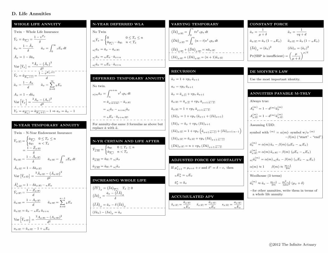
D. Life Annuities

WHOLE LIFE ANNUITY

Twin – Whole Life Insurance

Yx = aTx=

1− vTx

δ

ax =1− Axδ

ax =

∫ ∞0

tEx dt

Ax = 1− δax

Var[Yx]

=2Ax −

(Ax)2

δ2

Yx = aKx+1 =1− vKx+1

d

ax =1−Axd

ax =

∞∑k=0

kEx

Ax = 1− dax

Var[Yx]

=2Ax − (Ax)2

d2

Yx = aKx= aKx+1 − 1⇒ ax = ax − 1

N-YEAR TEMPORARY ANNUITY

Twin – N-Year Endowment Insurance

Yx:n =

{aTx

0 ≤ Tx ≤ nan n < Tx

=1− Zx:n

δ

ax:n =1− Ax:n

δax:n =

∫ n

0tEx dt

Ax:n = 1− δax:n

Var[Yx:n

]=

2Ax:n −(Ax:n

)2δ2

A1x:n = 1− δax:n − nEx

Yx:n =1− Zx:n

d

ax:n =1−Ax:n

dax:n =

n−1∑k=0

kEx

ax:n = ax − nEx ax+n

Var[Yx:n

]=

2Ax:n − (Ax:n )2

d2

ax:n = ax:n − 1 + nEx

N-YEAR DEFERRED WLA

No Twin

n|Yx =

{0 0 ≤ Tx ≤ naTx

− an n < Tx

n|ax = ax − ax:n

n|ax = nEx · ax+n

n|ax = nEx · ax+n

DEFERRED TEMPORARY ANNUITY

No twin.

n|max =

∫ n+m

nvt tpx dt

= ax:n+m − ax:n

= n|ax − n+m|ax

= nEx · ax+n:m

For annuity-due same 3 formulas as above butreplace a with a.

N-YR CERTAIN AND LIFE AFTER

Yx:n =

{an 0 ≤ Tx ≤ naTx

n < Tx

ax:n = an + n|ax

ax:n = an + n|ax

INCREASING WHOLE LIFE(IY)x

=(I a)Tx

Tx ≥ 0(I a)x

=ax −

(IA)x

δ(IA)x

= ax − δ(I a)x

(Iax)− (Ia)x = ax

VARYING TEMPORARY(I a)x:n

=

∫ n

0tvt tpx dt(

Da)x:n

=

∫ n

0(n− t)vt tpx dt(

I a)x:n

+(Da)x:n

= nax:n

(Ia)x:n + (Da)x:n = (n+ 1)ax:n

RECURSION

ax = 1 + vpx ax+1

ax = vpx ax+1

ax = ax:1 + vpx ax+1

ax:n = ax:1 + vpx ax+1:n−1

ax:n = 1 + vpx ax+1:n−1

(Ia)x = 1 + vpx (ax+1 + (Ia)x+1)

(Ia)x = ax + vpx (Ia)x+1

(Ia)x:n = 1 + vpx(ax+1:n−1 + (Ia)x+1:n−1

)(Ia)x:n = ax:n + vpx (Ia)x+1:n−1

(Da)x:n = n+ vpx (Da)x+1:n−1

ADJUSTED FORCE OF MORTALITY

If µ∗x+t = µx+t + c and δ∗ = δ − c, then

nE∗x = nEx

a∗x = ax

ACCUMULATED APV

sx:n =ax:n

nExsx:n =

ax:n

nExsx:n =

ax:n

nEx

CONSTANT FORCE

ax =1

µ+ δax =

1

vq + d

ax:n = ax (1− nEx) ax:n = ax (1− nEx)(I a)x

= (ax)2 (Ia)x = (ax)2

Pr(SBP is insufficient) =

(µ

µ+ δ

)µ/δ

DE MOIVRE’S LAW

Use the most important identity.

ANNUITIES PAYABLE M-THLY

Always true:

A(m)x = 1− d(m)a

(m)x

A(m)x:n = 1− d(m)a

(m)x:n

Assuming UDD:

symbol with (m) = α(m)· symbol w/o (m)

−β(m) (“start” - “end”)

a(m)x = α(m) ax − β(m) (0Ex −∞Ex)

a(m)x:n = α(m) ax:n − β(m) (0Ex − nEx)

n|a(m)x = α(m) n|ax − β(m) (nEx −∞Ex)

α(m) ≈ 1 β(m) ≈ m−12m

Woolhouse (3 terms)

a(m)x ≈ ax − m−1

2m− m2−1

12m2 (µx + δ)

−for other annuities, write them in terms ofa whole life annuity


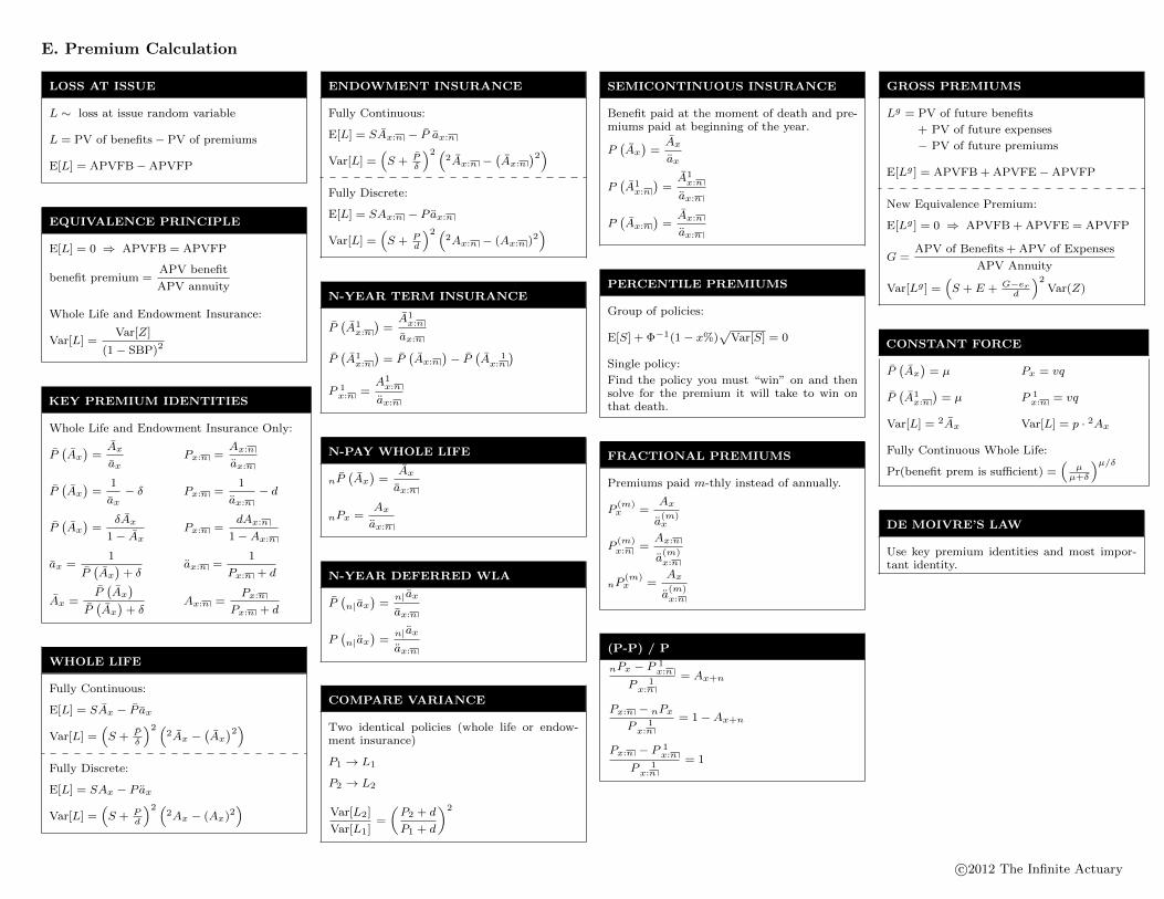
E. Premium Calculation

LOSS AT ISSUE

L ∼ loss at issue random variable

L = PV of benefits− PV of premiums

E[L] = APVFB−APVFP

EQUIVALENCE PRINCIPLE

E[L] = 0 ⇒ APVFB = APVFP

benefit premium =APV benefit

APV annuity

Whole Life and Endowment Insurance:

Var[L] =Var[Z]

(1− SBP)2

KEY PREMIUM IDENTITIES

Whole Life and Endowment Insurance Only:

P(Ax)

=Ax

axPx:n =

Ax:n

ax:n

P(Ax)

=1

ax− δ Px:n =

1

ax:n− d

P(Ax)

=δAx

1− AxPx:n =

dAx:n

1−Ax:n

ax =1

P(Ax)

+ δax:n =

1

Px:n + d

Ax =P(Ax)

P(Ax)

+ δAx:n =

Px:n

Px:n + d

WHOLE LIFE

Fully Continuous:

E[L] = SAx − P ax

Var[L] =(S + P

δ

)2 (2Ax −

(Ax)2)

Fully Discrete:

E[L] = SAx − P ax

Var[L] =(S + P

d

)2 (2Ax − (Ax)2

)

ENDOWMENT INSURANCE

Fully Continuous:

E[L] = SAx:n − P ax:n

Var[L] =(S + P

δ

)2 (2Ax:n −

(Ax:n

)2)Fully Discrete:

E[L] = SAx:n − P ax:n

Var[L] =(S + P

d

)2 (2Ax:n − (Ax:n )2

)

N-YEAR TERM INSURANCE

P(A1x:n

)=A1x:n

ax:n

P(A1x:n

)= P

(Ax:n

)− P

(A 1x:n

)P 1x:n =

A1x:n

ax:n

N-PAY WHOLE LIFE

nP(Ax)

=Ax

ax:n

nPx =Ax

ax:n

N-YEAR DEFERRED WLA

P(n|ax

)=

n|ax

ax:n

P(n|ax

)=

n|ax

ax:n

COMPARE VARIANCE

Two identical policies (whole life or endow-ment insurance)

P1 → L1

P2 → L2

Var[L2]

Var[L1]=

(P2 + d

P1 + d

)2

SEMICONTINUOUS INSURANCE

Benefit paid at the moment of death and pre-miums paid at beginning of the year.

P(Ax)

=Ax

ax

P(A1x:n

)=A1x:n

ax:n

P(Ax:n

)=Ax:n

ax:n

PERCENTILE PREMIUMS

Group of policies:

E[S] + Φ−1(1− x%)√

Var[S] = 0

Single policy:

Find the policy you must “win” on and thensolve for the premium it will take to win onthat death.

FRACTIONAL PREMIUMS

Premiums paid m-thly instead of annually.

P(m)x =

Ax

a(m)x

P(m)x:n =

Ax:n

a(m)x:n

nP(m)x =

Ax

a(m)x:n

(P-P) / P

nPx − P 1x:n

P 1x:n

= Ax+n

Px:n − nPx

P 1x:n

= 1−Ax+n

Px:n − P 1x:n

P 1x:n

= 1

GROSS PREMIUMS

Lg = PV of future benefits

+ PV of future expenses

− PV of future premiums

E[Lg ] = APVFB + APVFE−APVFP

New Equivalence Premium:

E[Lg ] = 0 ⇒ APVFB + APVFE = APVFP

G =APV of Benefits + APV of Expenses

APV Annuity

Var[Lg ] =(S + E + G−er

d

)2Var(Z)

CONSTANT FORCE

P(Ax)

= µ Px = vq

P(A1x:n

)= µ P 1

x:n = vq

Var[L] = 2Ax Var[L] = p · 2Ax

Fully Continuous Whole Life:

Pr(benefit prem is sufficient) =(

µµ+δ

)µ/δ

DE MOIVRE’S LAW

Use key premium identities and most impor-tant identity.


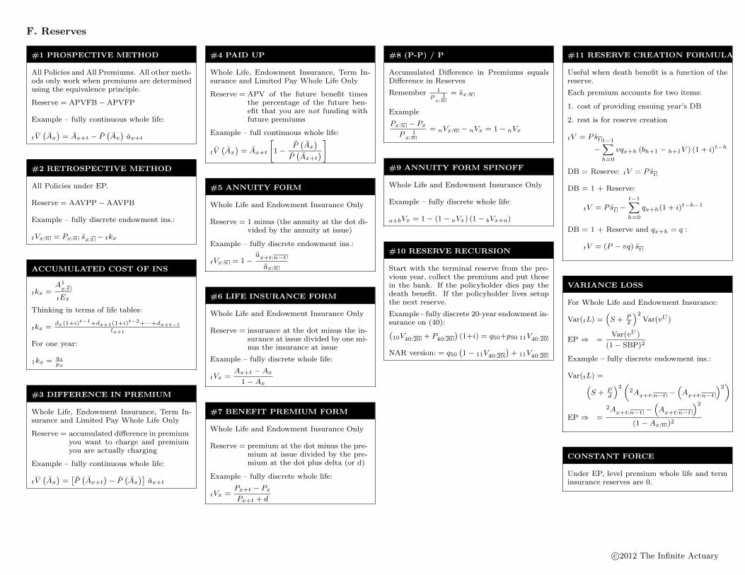
F. Reserves

#1 PROSPECTIVE METHOD

All Policies and All Premiums. All other meth-ods only work when premiums are determinedusing the equivalence principle.

Reserve = APVFB−APVFP

Example – fully continuous whole life:

tV(Ax)

= Ax+t − P(Ax)ax+t

#2 RETROSPECTIVE METHOD

All Policies under EP.

Reserve = AAVPP−AAVPB

Example – fully discrete endowment ins.:

tVx:n = Px:n sx:t − tkx

ACCUMULATED COST OF INS

tkx =A1x:t

tEx

Thinking in terms of life tables:

tkx =dx(1+i)t−1+dx+1(1+i)t−2+···+dx+t−1

lx+t

For one year:

1kx = qxpx

#3 DIFFERENCE IN PREMIUM

Whole Life, Endowment Insurance, Term In-surance and Limited Pay Whole Life Only

Reserve = accumulated difference in premiumyou want to charge and premiumyou are actually charging

Example – fully continuous whole life:

tV(Ax)

=[P(Ax+t

)− P

(Ax)]ax+t

#4 PAID UP

Whole Life, Endowment Insurance, Term In-surance and Limited Pay Whole Life Only

Reserve = APV of the future benefit timesthe percentage of the future ben-efit that you are not funding withfuture premiums

Example – full continuous whole life:

tV(Ax)

= Ax+t

[1−

P(Ax)

P(Ax+t

)]

#5 ANNUITY FORM

Whole Life and Endowment Insurance Only

Reserve = 1 minus (the annuity at the dot di-vided by the annuity at issue)


tVx:n = 1−ax+t:n−tax:n

#6 LIFE INSURANCE FORM


Reserve = insurance at the dot minus the in-surance at issue divided by one mi-nus the insurance at issue

Example – fully discrete whole life:

tVx =Ax+t −Ax

1−Ax

#7 BENEFIT PREMIUM FORM


Reserve = premium at the dot minus the pre-mium at issue divided by the pre-mium at the dot plus delta (or d)


tVx =Px+t − PxPx+t + d

#8 (P-P) / P

Accumulated Difference in Premiums equalsDifference in Reserves

Remember 1

P 1x:n

= sx:n

Example

Px:n − PxP 1x:n

= nVx:n − nVx = 1− nVx

#9 ANNUITY FORM SPINOFF



a+bVx = 1− (1− aVx) (1− bVx+a)

#10 RESERVE RECURSION

Start with the terminal reserve from the pre-vious year, collect the premium and put thosein the bank. If the policyholder dies pay thedeath benefit. If the policyholder lives setupthe next reserve.

Example - fully discrete 20-year endowment in-surance on (40):(10V40:20 + P40:20

)(1+i) = q50+p50 11V40:20

NAR version: = q50

(1− 11V40:20

)+ 11V40:20

#11 RESERVE CREATION FORMULA

Useful when death benefit is a function of thereserve.

Each premium accounts for two items:

1. cost of providing ensuing year’s DB

2. rest is for reserve creation

tV = P st

−t−1∑h=0

vqx+h (bh+1 − h+1V ) (1 + i)t−h

DB = Reserve: tV = P st

DB = 1 + Reserve:

tV = P st −t−1∑h=0

qx+h(1 + i)t−h−1

DB = 1 + Reserve and qx+h = q :

tV = (P − vq) st

VARIANCE LOSS

For Whole Life and Endowment Insurance:

Var(tL) =(S + P

δ

)2Var(vU )

EP ⇒ =Var(vU )

(1− SBP)2


Var(tL) =(S + P

d

)2(

2Ax+t:n−t −(Ax+t:n−t

)2)

EP ⇒ =

2Ax+t:n−t −(Ax+t:n−t

)2

(1−Ax:n )2

CONSTANT FORCE

Under EP, level premium whole life and terminsurance reserves are 0.


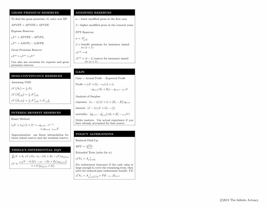
GROSS PREMIUM RESERVES

To find the gross premium, G, solve new EP

APVFP = APVFB + APVFE

Expense Reserves:

kVe = APVFE−APVFL

kVe = AAVPL−AAVPE

Gross Premium Reserve:

kVg = kV

n + kVe

Can also use recursion for expense and grosspremium reserves.

SEMI-CONTINUOUS RESERVES

Assuming UDD

tV(Ax)

= iδ tVx

tV(A1x:n

)= i

δ tV 1x:n

tV(Ax:n

)= i

δ tV 1x:n + tV 1

x:n

INTERIM BENEFIT RESERVES

Exact Method:

(hV + πh) (1 + i)s = sqx+h · v1−s

+spx+h · h+sV

Approximation: use linear interpolation be-tween initial reserve and the terminal reserve.

THIELE’S DIFFERENTIAL EQN

ddt t

V = δt ·tV +Gt−et−(St + Et − tV )µ[x]+t

tV ≈t+hV − h

(Gt − et − (St + Et)µ[x]+t

)1 + h

(µ[x]+t + δt

)

MODIFIED RESERVES

α− lower modified prem in the first year

β−higher modified prem in the renewal years

FPT Reserves:

α = A1x:1

β = benefit premium for insurance issuedto (x+ 1)

1Vm = 0

tVm = (t− 1) reserve for insurance issuedto (x+ 1)

GAIN

Gain = Actual Profit− Expected Profit

Profit = (tV +Gt − et) (1 + i)

−qx+t (St + Et)− px+t · t+1V

Analysis of Surplus:

expenses: (et − e′t) (1 + i) + (Et − E′t) qx+t

interest: (i′ − i) (tV +Gt − e′t)

mortality:(qx+t − q′x+t

)(St + E′t − t+1V )

Order matters. Use actual experience if youhave already accounted for that source.

POLICY ALTERATIONS

Reduced Paid-Up:

RPU = tCVxAx+t

Extended Term (solve for n):

tCVx = A 1x+t:n

For endowment insurance if the cash value islarge enough to cover the remaining term, thensolve for reduced pure endowment benefit, PE

tCVx = A 1x+t:n−t + PE · n−tEx+t


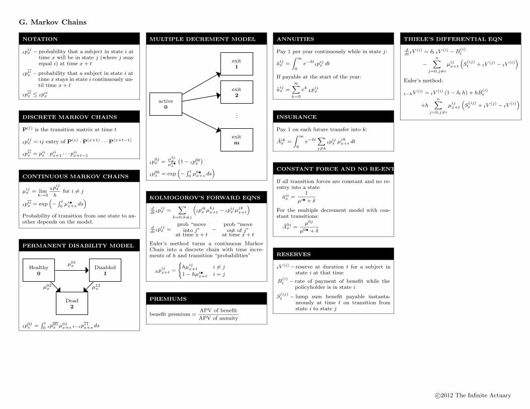
G. Markov Chains

NOTATION

tpijx − probability that a subject in state i at

time x will be in state j (where j mayequal i) at time x+ t

tpiix − probability that a subject in state i attime x stays in state i continuously un-til time x+ t

tpiix ≤ tpiix

DISCRETE MARKOV CHAINS

P(t) is the transition matrix at time t

tpijx = ij entry of P(x) ·P(x+1) · · ·P(x+t−1)

tpiix = piix · piix+1 · · · piix+t−1

CONTINUOUS MARKOV CHAINS

µijx = limh→0

hpijx

hfor i 6= j

tpiix = exp(−∫ t0 µ

i•x+s ds

)Probability of transition from one state to an-other depends on the model.

PERMANENT DISABILITY MODEL

Healthy0

Disabled1

Dead2

µ01x

µ02x µ12x

tp01x =∫ t0 sp

00x µ01x+s t−sp

11x+s ds

MULTIPLE DECREMENT MODEL

active0

exit1

exit2

exitm

tp0jx =

µ0jxµ0•x

(1− tp00x

)tp00x = exp

(−∫ t0 µ

0•x+s ds

)

KOLMOGOROV’S FORWARD EQNS

ddt t

pijx =∑

k=0,k 6=j

(tpikx µ

kjx+t − tp

ijx µ

jkx+t

)ddt t

pijx =prob “move

into j”at time x+ t

−prob “move

out of j”at time x+ t

Euler’s method turns a continuous MarkovChain into a discrete chain with time incre-ments of h and transition “probabilities”

hpijx+t =

{hµijx+t i 6= j

1− hµi•x+t i = j

PREMIUMS

benefit premium =APV of benefit

APV of annuity

ANNUITIES

Pay 1 per year continuously while in state j:

aijx =

∫ ∞0

e−δttpijx dt

If payable at the start of the year:

aijx =

∞∑k=0

vk kpijx

INSURANCE

Pay 1 on each future transfer into k:

Aikx =

∫ ∞0

e−δt∑j 6=k

tpijx µ

jkx+t dt

CONSTANT FORCE AND NO RE-ENTRY

If all transition forces are constant and no re-entry into a state

aiix =1

µi• + δ

For the multiple decrement model with con-stant transitions:

A0jx =

µ0j

µ0• + δ

RESERVES

tV (i)− reserve at duration t for a subject instate i at that time

B(i)t − rate of payment of benefit while the

policyholder is in state i

S(ij)t − lump sum benefit payable instanta-

neously at time t on transition fromstate i to state j

THIELE’S DIFFERENTIAL EQN

ddt t

V (i) = δt tV (i) −B(i)t

−n∑

j=0,j 6=iµijx+t

(S(ij)t + tV

(j) − tV(i))

Euler’s method:

t−hV(i) = tV (i) (1− δt h) + hB

(i)t

+hn∑

j=0,j 6=iµijx+t

(S(ij)t + tV

(j) − tV(i))


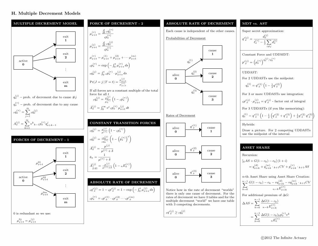
H. Multiple Decrement Models

MULTIPLE DECREMENT MODEL

active0

exit1

exit2

exitm

q(j)x − prob. of decrement due to cause #j

q(τ)x − prob. of decrement due to any cause

tq(τ)x =

m∑j=1

tq(j)x

A(j)x =

∞∑k=1

vkk−1p(τ)x qjx+k−1

FORCES OF DECREMENT - 1

active0

exit1

exit2

exitm

µ01x+t

µ02x+t

µ0mx+t

0 is redundant so we use:

µ0jx+t = µ(j)x+t

FORCE OF DECREMENT - 2

µ(τ)x+t =

ddt t

q(τ)x

tp(τ)x

µ(j)x+t =

ddt t

q(j)x

tp(τ)x

µ(τ)x+t = µ

(1)x+t + µ

(2)x+t + · · ·µ(m)

x+t

tp(τ)x = exp

(−∫ t0 µ

(τ)x+s ds

)tq

(j)x =

∫ t0 sp

(τ)x · µ(j)x+s ds

Pr(J = j |T = t) =µ(j)x+t

µ(τ)x+t

If all forces are a constant multiple of the totalforce for all t

tq(j)x = µ

(j)x

µ(τ)x

(1− tp

(τ)x

)A

(j)x =

∫∞0 vt tp

(τ)x µ

(j)x+t dt

CONSTANT TRANSITION FORCES

tq(j)x = µ(j)

µ(τ)

(1− tp

(τ)x

)tq

(j)x = tq

(j)x

tq(τ)x

(1−

(p(τ)x

)t)A

(j)x =

µ(j)

µ(τ) + δ

ax =1

µ(τ) + δ

A(j)1x:n

= µ(j)

µ(τ)+δ

(1− nE

(τ)x

)

ABSOLUTE RATE OF DECREMENT

tq′(j)x = 1− tp′

(j)x = 1− exp

(−∫ t0 µ

(j)x+s ds

)tp

(τ)x = tp′

(1)x · tp′

(2)x · · · tp′

(m)x

ABSOLUTE RATE OF DECREMENT

Each cause is independent of the other causes.

Probabilities of Decrement

alive0

cause1

cause2

cause3

q(1)x

q(2)x

q(3)x

Rates of Decrement

alive0

cause1

alive0

cause2

alive0

cause3

q′(1)x

q′(2)x

q′(3)x

Notice how in the rate of decrement “worlds”there is only one cause of decrement. For therates of decrement we have 3 tables and for themultiple decrement “world” we have one tablewith 3 competing decrements.

tq′(j)x ≥ tq

(j)x

MDT vs. AST

Super secret approximation:

q′(j)x =d(j)x

`(τ)x − 1

2

∑i6=j

d(i)x

Constant Force and UDDMDT:

p′(j)x =(p(τ)x

)q(j)x /q(τ)x

UDDAST:

For 2 UDDASTs use the midpoint:

q(1)x = q′(1)x

(1− 1

2q′(2)x

)For 3 or more UDDASTs use integration:

tp′(j)x · µ

(j)x+t = q′(j)x - factor out of integral

For 3 UDDASTs (if you like memorizing):

q(1)x = q′(1)x

(1− 1

2

(q′(2)x + q′(3)x

)+ 1

3q′(2)x q′(3)x

)Hybrids:

Draw a picture. For 2 competing UDDASTsuse the midpoint of the interval.

ASSET SHARE

Recursion:

[kAS +G(1− ck)− ek] (1 + i)

= q(d)x+k + q

(w)x+k · k+1CV + p

(τ)x+k · k+1AS

n-th Asset Share using Asset Share Creation:

n−1∑k=0

G(1− ck)− ek − vq(d)x+k − vq

(w)x+k · k+1CV

n−kE(τ)x+k

For additional premium of ∆G:

∆AS =

n−1∑k=0

∆G(1− ck)

n−kE(τ)x+k

=

n−1∑k=0

∆G(1− ck)kp(τ)x vk

nE(τ)x


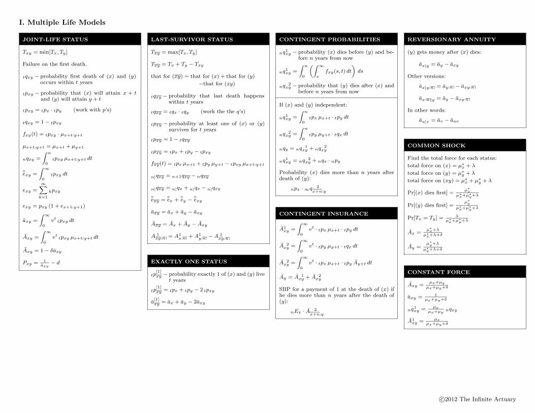
I. Multiple Life Models

JOINT-LIFE STATUS

Txy = min[Tx, Ty ]

Failure on the first death.

tqxy − probability first death of (x) and (y)occurs within t years

tpxy − probability that (x) will attain x + tand (y) will attain y + t

tpxy = tpx · tpy (work with p’s)

tqxy = 1 − tpxy

fxy(t) = tpxy · µx+t:y+t

µx+t:y+t = µx+t + µy+t

nqxy =

∫ n

0tpxy µx+t:y+t dt

◦exy =

∫ ∞0

tpxy dt

exy =∞∑k=1

kpxy

exy = pxy (1 + ex+1:y+1)

axy =

∫ ∞0

vt tpxy dt

Axy =

∫ ∞0

vt tpxy µx+t:y+t dt

Axy = 1 − δaxy

Pxy = 1axy

− d

LAST-SURVIVOR STATUS

Txy = max[Tx, Ty ]

Txy = Tx + Ty − Txy

that for (xy) = that for (x) + that for (y)

−that for (xy)

tqxy − probability that last death happenswithin t years

tqxy = tqx · tqy (work the the q’s)

tpxy − probability at least one of (x) or (y)survives for t years

tpxy = 1 − tqxy

tpxy = tpx + tpy − tpxy

fxy(t) = tpx µx+t + tpy µy+t − tpxy µx+t:y+t

n|qxy = n+1qxy − nqxy

n|qxy = n|qx + n|qx − n|qxy

◦exy =

◦ex +

◦ey − ◦exy

axy = ax + ay − axy

Axy = Ax + Ay − Axy

A 1xy:n = A1

x:n +A1y:n −A 1

xy:n

EXACTLY ONE STATUS

tp[1]xy − probability exactly 1 of (x) and (y) live

t years

tp[1]xy = tpx + tpy − 2 tpxy

a[1]xy = ax + ay − 2axy

CONTINGENT PROBABILITIES

nq1xy − probability (x) dies before (y) and be-fore n years from now

nq1xy =

∫ n

0

(∫ ∞s

fxy(s, t) dt

)ds

nq 2xy − probability that (y) dies after (x) and

before n years from now

If (x) and (y) independent:

nq1xy =

∫ n

0tpx µx+t · tpy dt

nq 2xy =

∫ n

0tpy µy+t · tqx dt

nqy = nq 1xy + nq 2

xy

nq1xy = nq 2xy + nqx · npy

Probability (x) dies more than n years afterdeath of (y):

npx ·∞q 2x+n:y

CONTINGENT INSURANCE

A1xy =

∫ ∞0

vt · tpx µx+t · tpy dt

A 2xy =

∫ ∞0

vt · tpy µy+t · tqx dt

A 2xy =

∫ ∞0

vt · tpx µx+t · tpy Ay+t dt

Ay = A 1xy + A 2

xy

SBP for a payment of 1 at the death of (x) ifhe dies more than n years after the death of(y):

nEx · A 2x+n:y

REVERSIONARY ANNUITY

(y) gets money after (x) dies:

ax|y = ay − axy

Other versions:

ax|y:n = ay:n − axy:n

ax:n |y = ay − axy:n

In other words:

au|v = av − auv

COMMON SHOCK

Find the total force for each status:

total force on (x) = µ∗x + λ

total force on (y) = µ∗y + λ

total force on (xy) = µ∗x + µ∗y + λ

Pr[(x) dies first] =µ∗x

µ∗x+µ∗

y+λ

Pr[(y) dies first] =µ∗y

µ∗x+µ∗

y+λ

Pr[Tx = Ty ] = λµ∗x+µ∗

y+λ

Ax =µ∗x+λ

µ∗x+λ+δ

Ay =µ∗y+λ

µ∗y+λ+δ

CONSTANT FORCE

Axy =µx+µy

µx+µy+δ

axy = 1µx+µy+δ

nq1xy = µxµx+µy

nqxy

A1xy = µx

µx+µy+δ


DE MOIVRE’S LAW

◦exx = ω−x

3

◦exy = y−xpx·

◦eyy +y−xqx·

◦ey

nq 2xy = 1

2 nqxy

A1xy =

ay:ω−x

ω − x


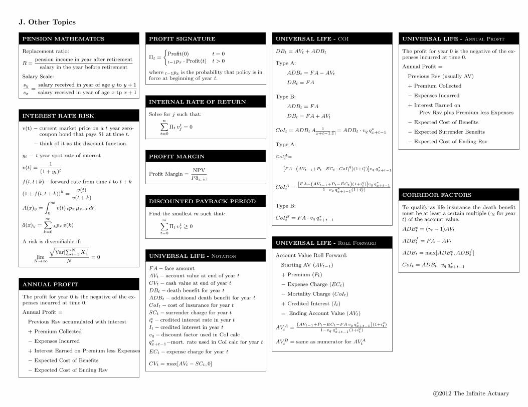
J. Other Topics

PENSION MATHEMATICS

Replacement ratio:

R =pension income in year after retirement

salary in the year before retirement

Salary Scale:

sy

sx=

salary received in year of age y to y + 1

salary received in year of age x tp x+ 1

INTEREST RATE RISK

v(t) − current market price on a t year zero-coupon bond that pays $1 at time t.

− think of it as the discount function.

yt − t year spot rate of interest

v(t) =1

(1 + yt)t

f(t, t+k)− forward rate from time t to t+ k

(1 + f(t, t+ k))k =v(t)

v(t+ k)

A(x)y =

∫ ∞0

v(t) tpx µx+t dt

a(x)y =

∞∑k=0

kpx v(k)

A risk is diversifiable if:

limN→∞

√Var[

∑Ni=1Xi]

N= 0

ANNUAL PROFIT

The profit for year 0 is the negative of the ex-penses incurred at time 0.

Annual Profit =

Previous Rsv accumulated with interest

+ Premium Collected

− Expenses Incurred

+ Interest Earned on Premium less Expenses

− Expected Cost of Benefits

− Expected Cost of Ending Rsv

PROFIT SIGNATURE

Πt =

{Profit(0) t = 0

t−1px · Profit(t) t > 0

where t−1px is the probability that policy is inforce at beginning of year t.

INTERNAL RATE OF RETURN

Solve for j such that:n∑

t=0

Πt vtj = 0

PROFIT MARGIN

Profit Margin =NPV

P ax:n

DISCOUNTED PAYBACK PERIOD

Find the smallest m such that:m∑t=0

Πt vtr ≥ 0

UNIVERSAL LIFE - Notation

FA− face amount

AVt − account value at end of year t

CVt − cash value at end of year t

DBt − death benefit for year t

ADBt − additional death benefit for year t

CoIt − cost of insurance for year t

SCt − surrender charge for year t

ict − credited interest rate in year t

It − credited interest in year t

vq − discount factor used in CoI calc

q∗x+t−1−mort. rate used in CoI calc for year t

ECt − expense charge for year t

CVt = max[AVt − SCt, 0]

UNIVERSAL LIFE - COI

DBt = AVt +ADBt

Type A:

ADBt = FA−AVt

DBt = FA

Type B:

ADBt = FA

DBt = FA+AVt

CoIt = ADBt A 1x+t−1:1

= ADBt · vq q∗x+t−1

Type A:

CoIAt =

[FA−(AVt−1+Pt−ECt−CoIAt )(1+ict )]vq q∗x+t−1

CoIAt =[FA−(AVt−1+Pt−ECt)(1+ict )]vq q∗x+t−1

1−vq q∗x+t−1(1+ict )

Type B:

CoIBt = FA · vq q∗x+t−1

UNIVERSAL LIFE - Roll Forward

Account Value Roll Forward:

Starting AV (AVt−1)

+ Premium (Pt)

− Expense Charge (ECt)

− Mortality Charge (CoIt)

+ Credited Interest (It)

= Ending Account Value (AVt)

AV At =

(AVt−1+Pt−ECt−FAvq q∗x+t−1)(1+ict )

1−vq q∗x+t−1(1+ict )

AV Bt = same as numerator for AV A

t

UNIVERSAL LIFE - Annual Profit

The profit for year 0 is the negative of the ex-penses incurred at time 0.

Annual Profit =

Previous Rsv (usually AV)

+ Premium Collected

− Expenses Incurred

+ Interest Earned on

Prev Rsv plus Premium less Expenses

− Expected Cost of Benefits

− Expected Surrender Benefits

− Expected Cost of Ending Rsv

CORRIDOR FACTORS

To qualify as life insurance the death benefitmust be at least a certain multiple (γt for yeart) of the account value.

ADBct = (γt − 1)AVt

ADBft = FA−AVt

ADBt = max[ADBct , ADB

ft ]

CoIt = ADBt · vq q∗x+t−1


Documents

TIA MLC Formula Sheet