TI™ Calculator Technology Manual to Accompany

Prepared by

Diane Benner Harrisburg Area Community College, Harrisburg, PA

Australia • Brazil • Mexico • Singapore • United Kingdom • United States

Statistics Learning from Data

Roxy Peck California Polytechnic State University,

San Luis Obispo, CA

CG

r

l

Not For Sale

© C

enga

ge L

earn

ing.

All

right

s res

erve

d. N

o di

strib

utio

n al

low

ed w

ithou

t exp

ress

aut

horiz

atio

n.

© 2014 Cengage Learning. All Rights Reserved. May not be copied, scanned, or duplicated, in whole or in part, except for use as permitted in a license distributed with a certain product or service or otherwise on a password-protected website for classroom use.

iii

Contents* Chapter 0 ...........................................................................................................................................

Chapter 1 ...........................................................................................................................................

Chapter 2 ........................................................................................................................................... 9

Chapter ......................................................................................................................................... 2

Chapter 5 ......................................................................................................................................... 36

Chapter .........................................................................................................................................

Chapter ......... .............................................................................................................................. 4

Chapter 1 ....................................................................................................................................... 4

Chapter 1 .......................................................................................................................................

Chapter 1 .......................................................................................................................................

Chapter 1 .......................................................................................................................................

Chapter 1 .......................................................................................................................................

Chapter .........................................................................................................................................

5

6

1

5

3 0

4 28

6 39

9 .. 5

0 9

1 51

2 5

3 58

5 4

* Chapters 7, 8 and 14 have been omitted from this guide since they contain no material relevant to Excel.

Not For Sale

© C

enga

ge L

earn

ing.

All

right

s res

erve

d. N

o di

strib

utio

n al

low

ed w

ithou

t exp

ress

aut

horiz

atio

n.

1

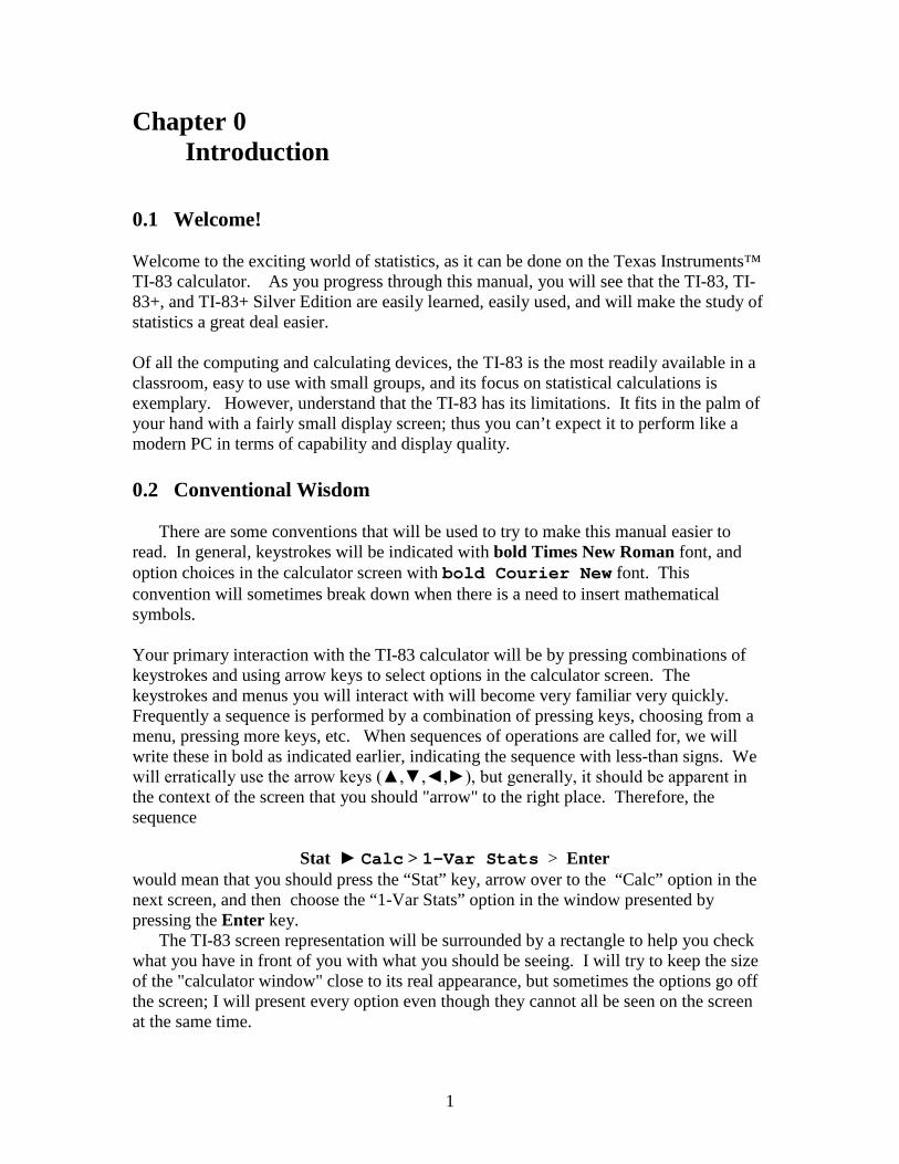
Chapter 0 Introduction 0.1 Welcome! Welcome to the exciting world of statistics, as it can be done on the Texas Instruments™ TI-83 calculator. As you progress through this manual, you will see that the TI-83, TI-83+, and TI-83+ Silver Edition are easily learned, easily used, and will make the study of statistics a great deal easier. Of all the computing and calculating devices, the TI-83 is the most readily available in a classroom, easy to use with small groups, and its focus on statistical calculations is exemplary. However, understand that the TI-83 has its limitations. It fits in the palm of your hand with a fairly small display screen; thus you can’t expect it to perform like a modern PC in terms of capability and display quality. 0.2 Conventional Wisdom

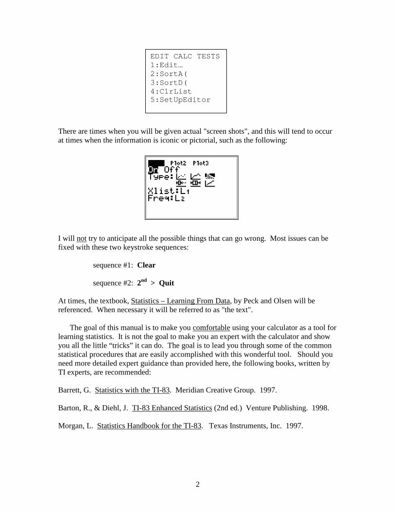
There are some conventions that will be used to try to make this manual easier to read. In general, keystrokes will be indicated with bold Times New Roman font, and option choices in the calculator screen with bold Courier New font. This convention will sometimes break down when there is a need to insert mathematical symbols. Your primary interaction with the TI-83 calculator will be by pressing combinations of keystrokes and using arrow keys to select options in the calculator screen. The keystrokes and menus you will interact with will become very familiar very quickly. Frequently a sequence is performed by a combination of pressing keys, choosing from a menu, pressing more keys, etc. When sequences of operations are called for, we will write these in bold as indicated earlier, indicating the sequence with less-than signs. We will erratically use the arrow keys (▲,▼,◄,►), but generally, it should be apparent in the context of the screen that you should "arrow" to the right place. Therefore, the sequence Stat ► Calc > 1-Var Stats > Enter would mean that you should press the “Stat” key, arrow over to the “Calc” option in the next screen, and then choose the “1-Var Stats” option in the window presented by pressing the Enter key. The TI-83 screen representation will be surrounded by a rectangle to help you check what you have in front of you with what you should be seeing. I will try to keep the size of the "calculator window" close to its real appearance, but sometimes the options go off the screen; I will present every option even though they cannot all be seen on the screen at the same time.

2

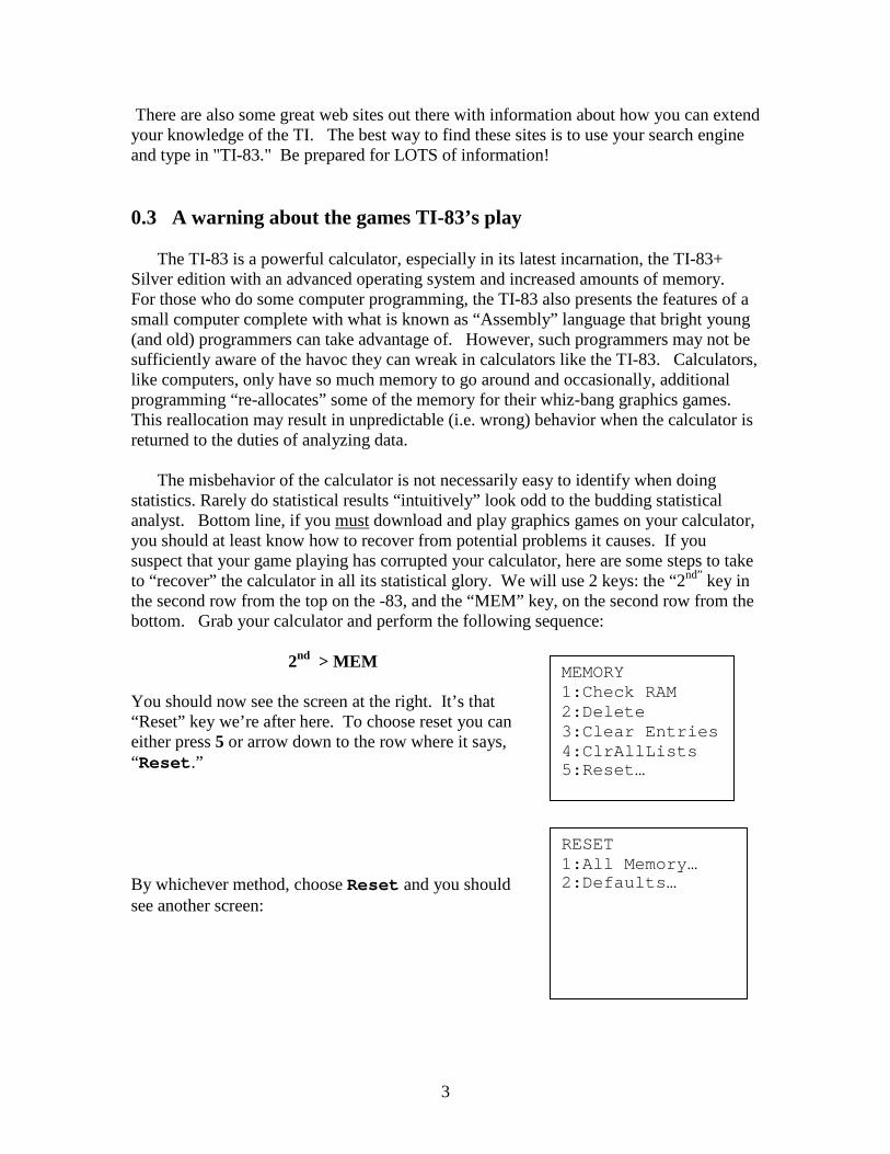
There are times when you will be given actual "screen shots", and this will tend to occur at times when the information is iconic or pictorial, such as the following: I will not try to anticipate all the possible things that can go wrong. Most issues can be fixed with these two keystroke sequences: sequence #1: Clear sequence #2: 2nd > Quit At times, the textbook, Statistics – Learning From Data, by Peck and Olsen will be referenced. When necessary it will be referred to as "the text".

The goal of this manual is to make you comfortable using your calculator as a tool for

learning statistics. It is not the goal to make you an expert with the calculator and show you all the little “tricks” it can do. The goal is to lead you through some of the common statistical procedures that are easily accomplished with this wonderful tool. Should you need more detailed expert guidance than provided here, the following books, written by TI experts, are recommended: Barrett, G. Statistics with the TI-83. Meridian Creative Group. 1997. Barton, R., & Diehl, J. TI-83 Enhanced Statistics (2nd ed.) Venture Publishing. 1998. Morgan, L. Statistics Handbook for the TI-83. Texas Instruments, Inc. 1997.

EDIT CALC TESTS 1:Edit… 2:SortA( 3:SortD( 4:ClrList 5:SetUpEditor

3

MEMORY 1:Check RAM 2:Delete 3:Clear Entries 4:ClrAllLists 5:Reset…

RESET 1:All Memory… 2:Defaults…

There are also some great web sites out there with information about how you can extend your knowledge of the TI. The best way to find these sites is to use your search engine and type in "TI-83." Be prepared for LOTS of information! 0.3 A warning about the games TI-83’s play

The TI-83 is a powerful calculator, especially in its latest incarnation, the TI-83+ Silver edition with an advanced operating system and increased amounts of memory. For those who do some computer programming, the TI-83 also presents the features of a small computer complete with what is known as “Assembly” language that bright young (and old) programmers can take advantage of. However, such programmers may not be sufficiently aware of the havoc they can wreak in calculators like the TI-83. Calculators, like computers, only have so much memory to go around and occasionally, additional programming “re-allocates” some of the memory for their whiz-bang graphics games. This reallocation may result in unpredictable (i.e. wrong) behavior when the calculator is returned to the duties of analyzing data.

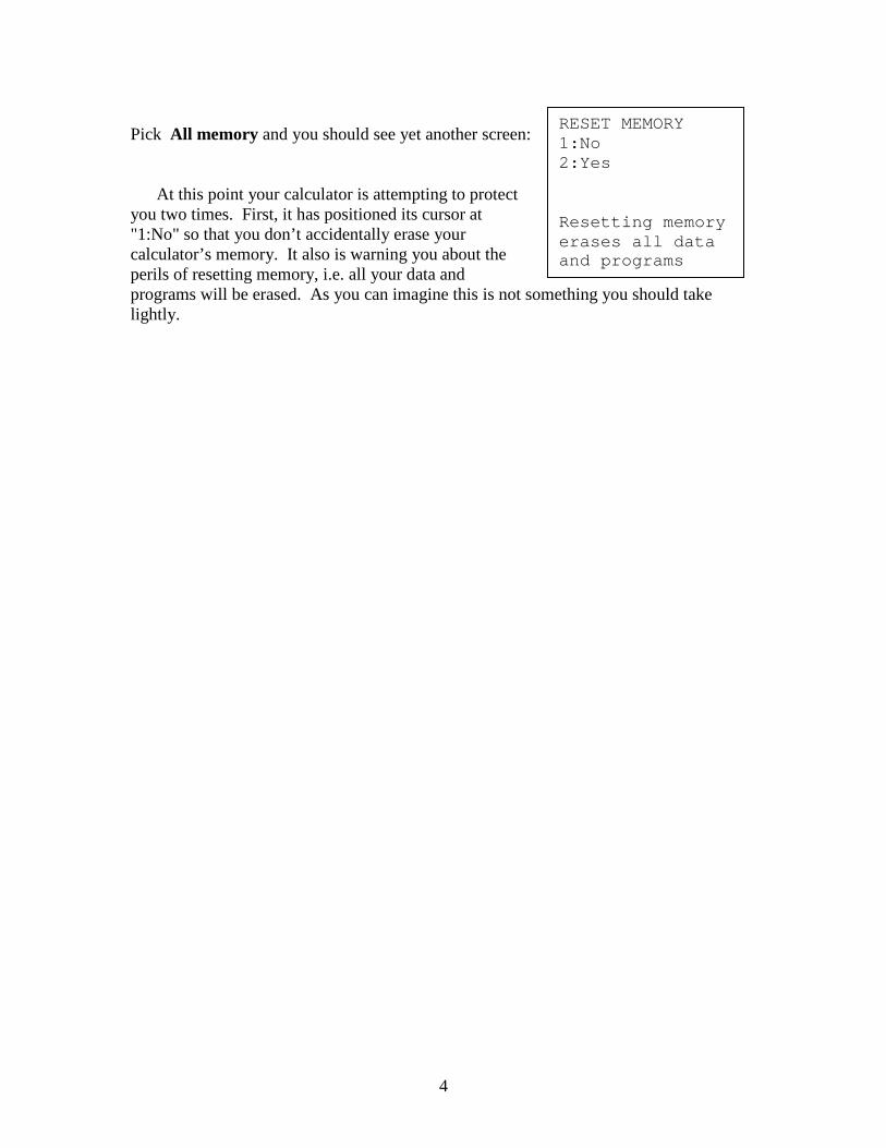
The misbehavior of the calculator is not necessarily easy to identify when doing statistics. Rarely do statistical results “intuitively” look odd to the budding statistical analyst. Bottom line, if you must download and play graphics games on your calculator, you should at least know how to recover from potential problems it causes. If you suspect that your game playing has corrupted your calculator, here are some steps to take to “recover” the calculator in all its statistical glory. We will use 2 keys: the “2nd” key in the second row from the top on the -83, and the “MEM” key, on the second row from the bottom. Grab your calculator and perform the following sequence: 2nd > MEM You should now see the screen at the right. It’s that “Reset” key we’re after here. To choose reset you can either press 5 or arrow down to the row where it says, “Reset.” By whichever method, choose Reset and you should see another screen:

4

RESET MEMORY 1:No 2:Yes Resetting memory erases all data and programs

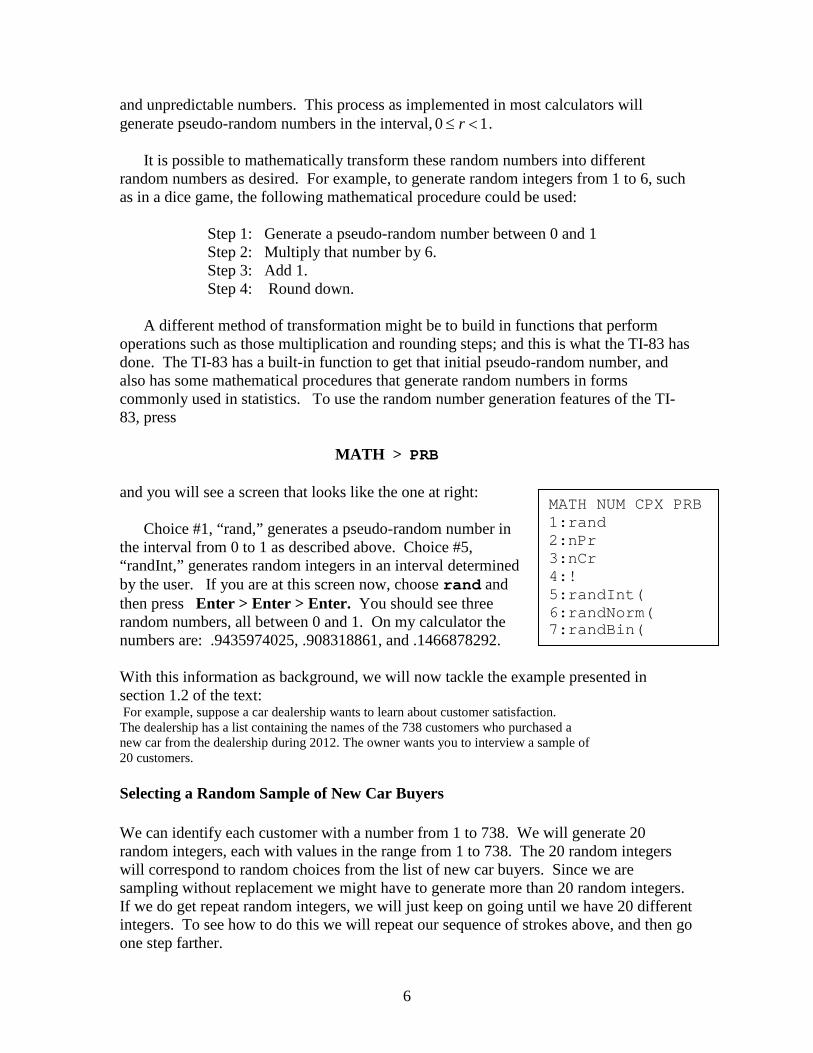
Pick All memory and you should see yet another screen: At this point your calculator is attempting to protect you two times. First, it has positioned its cursor at "1:No" so that you don’t accidentally erase your calculator’s memory. It also is warning you about the perils of resetting memory, i.e. all your data and programs will be erased. As you can imagine this is not something you should take lightly.

5

( )( )( )

1 2 1

1 1 2 2

2 1 2 3

#

# #

# #

seed magicNumber magicNumber pseudoRandom

pseudoRandom magicNumber magicNumber pseudoRandom

pseudoRandom magicNumber magicNumber pseudoRandom

× + →

× + →

× + →

Chapter 1 Collecting Data in Reasonable Ways 1.0 Introduction The topic of chapter 1 is the collection of data. Interpretation of data depends critically on how it was gathered. In some observational studies we may be interested only in describing the characteristics of a sample. In other circumstances the goal of the data gathering is to acquire a sample for the purpose of generalizing to a population. As an example, we may take a sample of high school students and ask the number of hours they spend studying in a typical week. Our purpose is not just to tabulate how many hours the students in the particular sample studied; we wish to generalize beyond the sample to the population of students. In order to make statements about the population, we must select the sample so that it has a good chance of “reflecting” the characteristics of the population. The critical aspect of sampling that enables us to generalize is that the sample is a “random” sample. There are different methods of random sampling, and each of them involves generating random numbers – it is at this stage the TI-83 enters the data gathering picture. 1.1 The random number generating capabilities of the TI-83. It seems odd to talk about computers or calculators generating “random” numbers – everybody knows that calculating machines operate by executing a step of pre-defined instructions. How can calculators generate random numbers? It turns out that calculators don’t actually produce truly random numbers; they produce what are known as “pseudo-random” numbers. The generation of pseudo-random numbers is accomplished by creating a sequence of numbers using a starting number, called a “seed.” The seed is built into the calculator in the factory, and everyone who has a TI-83 will start out in the same place with respect to pseudo-random numbers. (If you have a new TI-83 and have not generated any random numbers yet, find someone else with a new one and check it out.) The process works something like this…. and this sequence of pseudo-numbers continues generating numbers for a very long time before finally repeating itself. For our practical purposes the pseudo-random numbers generated by this process are just as good as actual random numbers. The “magic” numbers are not, of course, magic – they are numbers carefully chosen by mathematicians and computer science experts for the purpose of generating well shuffled

6

MATH NUM CPX PRB 1:rand 2:nPr 3:nCr 4:! 5:randInt( 6:randNorm( 7:randBin(

and unpredictable numbers. This process as implemented in most calculators will generate pseudo-random numbers in the interval, 0 1r≤ < .

It is possible to mathematically transform these random numbers into different random numbers as desired. For example, to generate random integers from 1 to 6, such as in a dice game, the following mathematical procedure could be used: Step 1: Generate a pseudo-random number between 0 and 1 Step 2: Multiply that number by 6. Step 3: Add 1. Step 4: Round down. A different method of transformation might be to build in functions that perform operations such as those multiplication and rounding steps; and this is what the TI-83 has done. The TI-83 has a built-in function to get that initial pseudo-random number, and also has some mathematical procedures that generate random numbers in forms commonly used in statistics. To use the random number generation features of the TI-83, press MATH > PRB and you will see a screen that looks like the one at right: Choice #1, “rand,” generates a pseudo-random number in the interval from 0 to 1 as described above. Choice #5, “randInt,” generates random integers in an interval determined by the user. If you are at this screen now, choose rand and then press Enter > Enter > Enter. You should see three random numbers, all between 0 and 1. On my calculator the numbers are: .9435974025, .908318861, and .1466878292. With this information as background, we will now tackle the example presented in section 1.2 of the text: For example, suppose a car dealership wants to learn about customer satisfaction. The dealership has a list containing the names of the 738 customers who purchased a new car from the dealership during 2012. The owner wants you to interview a sample of 20 customers. Selecting a Random Sample of New Car Buyers We can identify each customer with a number from 1 to 738. We will generate 20 random integers, each with values in the range from 1 to 738. The 20 random integers will correspond to random choices from the list of new car buyers. Since we are sampling without replacement we might have to generate more than 20 random integers. If we do get repeat random integers, we will just keep on going until we have 20 different integers. To see how to do this we will repeat our sequence of strokes above, and then go one step farther.

7

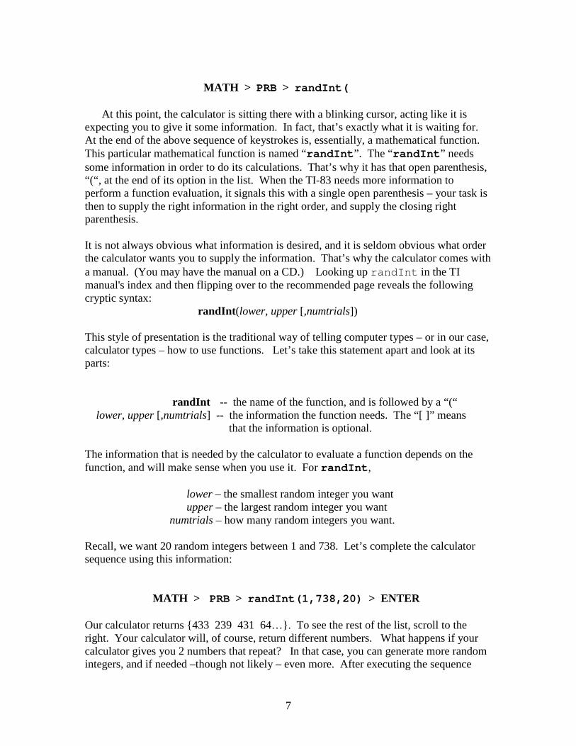
MATH > PRB > randInt(

At this point, the calculator is sitting there with a blinking cursor, acting like it is expecting you to give it some information. In fact, that’s exactly what it is waiting for. At the end of the above sequence of keystrokes is, essentially, a mathematical function. This particular mathematical function is named “randInt”. The “randInt” needs some information in order to do its calculations. That’s why it has that open parenthesis, “(“, at the end of its option in the list. When the TI-83 needs more information to perform a function evaluation, it signals this with a single open parenthesis – your task is then to supply the right information in the right order, and supply the closing right parenthesis. It is not always obvious what information is desired, and it is seldom obvious what order the calculator wants you to supply the information. That’s why the calculator comes with a manual. (You may have the manual on a CD.) Looking up randInt in the TI manual's index and then flipping over to the recommended page reveals the following cryptic syntax: randInt(lower, upper [,numtrials]) This style of presentation is the traditional way of telling computer types – or in our case, calculator types – how to use functions. Let’s take this statement apart and look at its parts: randInt -- the name of the function, and is followed by a “(“ lower, upper [,numtrials] -- the information the function needs. The “[ ]” means that the information is optional. The information that is needed by the calculator to evaluate a function depends on the function, and will make sense when you use it. For randInt, lower – the smallest random integer you want upper – the largest random integer you want numtrials – how many random integers you want. Recall, we want 20 random integers between 1 and 738. Let’s complete the calculator sequence using this information: MATH > PRB > randInt(1,738,20) > ENTER Our calculator returns {433 239 431 64…}. To see the rest of the list, scroll to the right. Your calculator will, of course, return different numbers. What happens if your calculator gives you 2 numbers that repeat? In that case, you can generate more random integers, and if needed –though not likely – even more. After executing the sequence

8

above, you don’t need to redo the whole sequence of keystrokes – just press ENTER again to execute the whole sequence of keystrokes on the TI-83.

At this point we have accomplished our goal – generating a random sample of size 20, from our population of new car buyers. 1.2 Afterword The TI-83 has a whole suite of random number generation capabilities. As you study different parts of probability and statistics, these functions can be very helpful. You might want to just browse in that chapter of your TI manual to see what's there.

9

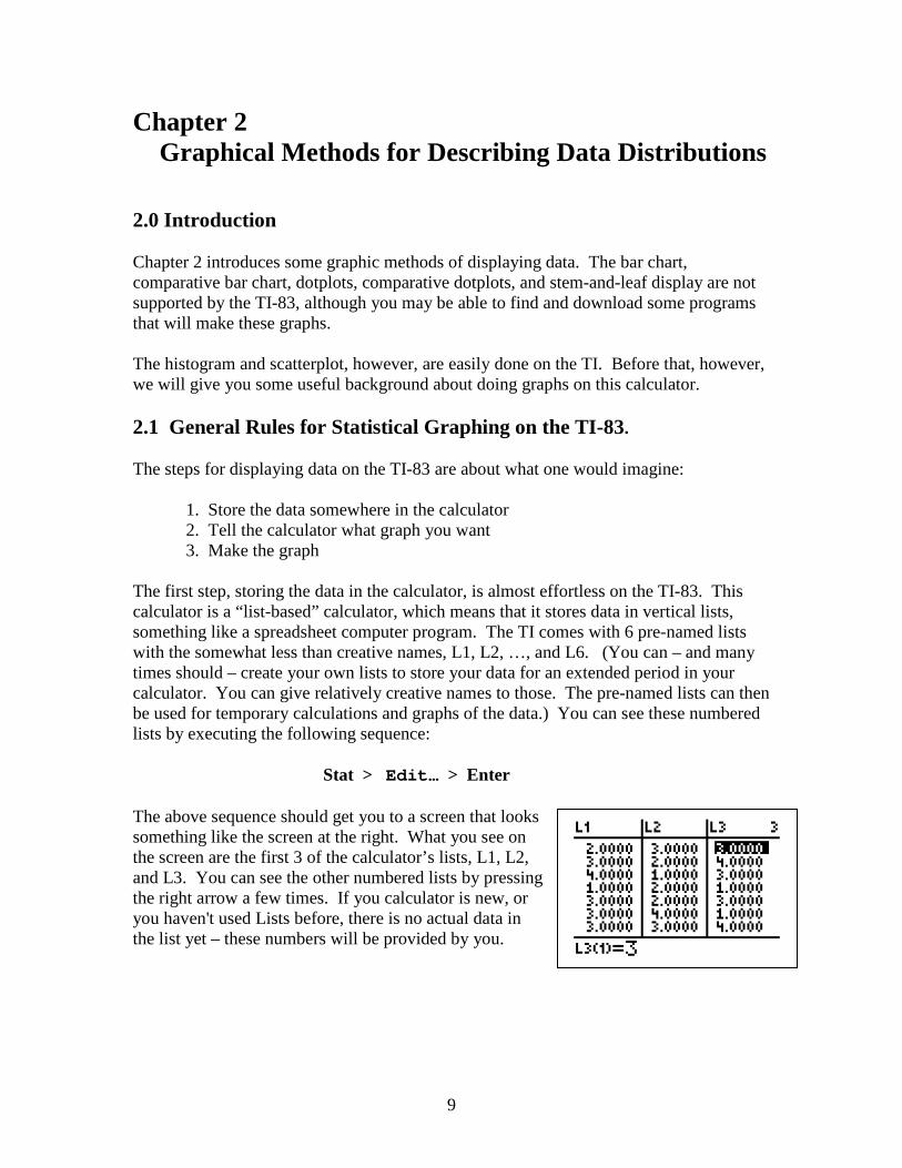
Chapter 2 Graphical Methods for Describing Data Distributions 2.0 Introduction Chapter 2 introduces some graphic methods of displaying data. The bar chart, comparative bar chart, dotplots, comparative dotplots, and stem-and-leaf display are not supported by the TI-83, although you may be able to find and download some programs that will make these graphs. The histogram and scatterplot, however, are easily done on the TI. Before that, however, we will give you some useful background about doing graphs on this calculator. 2.1 General Rules for Statistical Graphing on the TI-83. The steps for displaying data on the TI-83 are about what one would imagine: 1. Store the data somewhere in the calculator 2. Tell the calculator what graph you want 3. Make the graph The first step, storing the data in the calculator, is almost effortless on the TI-83. This calculator is a “list-based” calculator, which means that it stores data in vertical lists, something like a spreadsheet computer program. The TI comes with 6 pre-named lists with the somewhat less than creative names, L1, L2, …, and L6. (You can – and many times should – create your own lists to store your data for an extended period in your calculator. You can give relatively creative names to those. The pre-named lists can then be used for temporary calculations and graphs of the data.) You can see these numbered lists by executing the following sequence: Stat > Edit… > Enter The above sequence should get you to a screen that looks something like the screen at the right. What you see on the screen are the first 3 of the calculator’s lists, L1, L2, and L3. You can see the other numbered lists by pressing the right arrow a few times. If you calculator is new, or you haven't used Lists before, there is no actual data in the list yet – these numbers will be provided by you.

10

2.2 Entering data Example 2.13: Enrollments at Public Universities States differ widely in the percentage of college students who are enrolled in public institutions. The National Center for Education Statistics provided the accompanying data on this percentage for the 50 U.S. states for fall 2007.

Percentage of College Students Enrolled in Public Institutions

96 86 81 84 77 90 73 53 90 96 73 93 76 86 78 76 88 86 87 64 60 58 89 86 80 66 70 90 89 82 73 81 73 72 56 55 75 77 82 83 79 75 59 59 46 50 64 80 82 75

Be very careful here! You should NOT enter the data in rows and columns as you see

them presented here originally. These are data for one variable, and should be entered in one list, top to bottom.

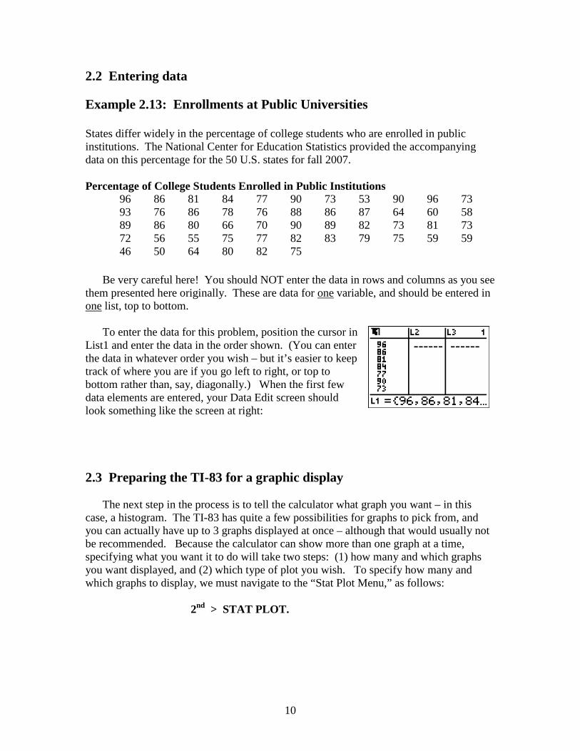
To enter the data for this problem, position the cursor in

List1 and enter the data in the order shown. (You can enter the data in whatever order you wish – but it’s easier to keep track of where you are if you go left to right, or top to bottom rather than, say, diagonally.) When the first few data elements are entered, your Data Edit screen should look something like the screen at right:

2.3 Preparing the TI-83 for a graphic display

The next step in the process is to tell the calculator what graph you want – in this case, a histogram. The TI-83 has quite a few possibilities for graphs to pick from, and you can actually have up to 3 graphs displayed at once – although that would usually not be recommended. Because the calculator can show more than one graph at a time, specifying what you want it to do will take two steps: (1) how many and which graphs you want displayed, and (2) which type of plot you wish. To specify how many and which graphs to display, we must navigate to the “Stat Plot Menu,” as follows: 2nd > STAT PLOT.

11

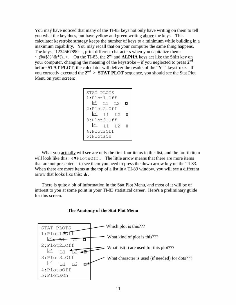
You may have noticed that many of the TI-83 keys not only have writing on them to tell you what the key does, but have yellow and green writing above the keys. This calculator keystroke strategy keeps the number of keys to a minimum while building in a maximum capability. You may recall that on your computer the same thing happens. The keys, `1234567890-=, print different characters when you capitalize them: ~!@#$%^&*()_+. On the TI-83, the 2nd and ALPHA keys act like the Shift key on your computer, changing the meaning of the keystroke – if you neglected to press 2nd before STAT PLOT, the calculator will deliver the results of the “Y=” keystroke. If you correctly executed the 2nd > STAT PLOT sequence, you should see the Stat Plot Menu on your screen:

What you actually will see are only the first four items in this list, and the fourth item will look like this: 4▼PlotsOff. The little arrow means that there are more items that are not presented – to see them you need to press the down arrow key on the TI-83. When there are more items at the top of a list in a TI-83 window, you will see a different arrow that looks like this: ▲.

There is quite a bit of information in the Stat Plot Menu, and most of it will be of interest to you at some point in your TI-83 statistical career. Here's a preliminary guide for this screen.

STAT PLOTS 1:Plot1…Off L1 L2 2:Plot2…Off L1 L2 3:Plot3…Off L1 L2 4:PlotsOff 5:PlotsOn

The Anatomy of the Stat Plot Menu Which plot is this??? What kind of plot is this??? What list(s) are used for this plot??? What character is used (if needed) for dots???

STAT PLOTS 1:Plot1…Off L1 L2 2:Plot2…Off L1 L2 3:Plot3…Off L1 L2 4:PlotsOff 5:PlotsOn

12

Plot1 Plot2 Plot3 On Off Type:

XList: 1L

YList: 2L

Mark:

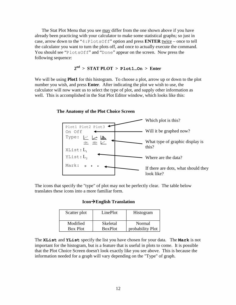
The Stat Plot Menu that you see may differ from the one shown above if you have already been practicing with your calculator to make some statistical graphs; so just in case, arrow down to the “4:PlotsOff” option and press ENTER twice – once to tell the calculator you want to turn the plots off, and once to actually execute the command. You should see “PlotsOff” and “Done” appear on the screen. Now press the following sequence: 2nd > STAT PLOT > Plot1…On > Enter We will be using Plot1 for this histogram. To choose a plot, arrow up or down to the plot number you wish, and press Enter. After indicating the plot we wish to use, the calculator will now want us to select the type of plot, and supply other information as well. This is accomplished in the Stat Plot Editor window, which looks like this: The Anatomy of the Plot Choice Screen The icons that specify the "type" of plot may not be perfectly clear. The table below translates these icons into a more familiar form. IconEnglish Translation

Scatter plot

LinePlot Histogram

Modified Box Plot

Skeletal BoxPlot

Normal probability Plot

The XList and YList specify the list you have chosen for your data. The Mark is not important for the histogram, but is a feature that is useful in plots to come. It is possible that the Plot Choice Screen doesn't look exactly like you see above. This is because the information needed for a graph will vary depending on the "Type" of graph.

Which plot is this? Will it be graphed now? What type of graphic display is this? Where are the data? If there are dots, what should they look like?

13

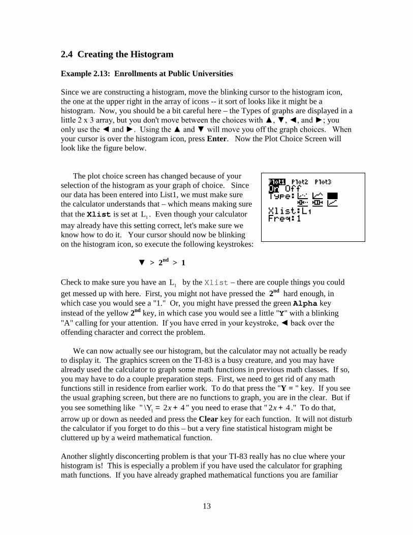
2.4 Creating the Histogram Example 2.13: Enrollments at Public Universities Since we are constructing a histogram, move the blinking cursor to the histogram icon, the one at the upper right in the array of icons -- it sort of looks like it might be a histogram. Now, you should be a bit careful here – the Types of graphs are displayed in a little 2 x 3 array, but you don't move between the choices with ▲, ▼, ◄, and ►; you only use the ◄ and ►. Using the ▲ and ▼ will move you off the graph choices. When your cursor is over the histogram icon, press Enter. Now the Plot Choice Screen will look like the figure below.

The plot choice screen has changed because of your selection of the histogram as your graph of choice. Since our data has been entered into List1, we must make sure the calculator understands that – which means making sure that the Xlist is set at 1L . Even though your calculator may already have this setting correct, let's make sure we know how to do it. Your cursor should now be blinking on the histogram icon, so execute the following keystrokes: ▼ > 2nd > 1 Check to make sure you have an 1L by the Xlist – there are couple things you could get messed up with here. First, you might not have pressed the 2nd hard enough, in which case you would see a "1." Or, you might have pressed the green Alpha key instead of the yellow 2nd key, in which case you would see a little "Y" with a blinking "A" calling for your attention. If you have erred in your keystroke, ◄ back over the offending character and correct the problem.

We can now actually see our histogram, but the calculator may not actually be ready to display it. The graphics screen on the TI-83 is a busy creature, and you may have already used the calculator to graph some math functions in previous math classes. If so, you may have to do a couple preparation steps. First, we need to get rid of any math functions still in residence from earlier work. To do that press the "Y = " key. If you see the usual graphing screen, but there are no functions to graph, you are in the clear. But if you see something like " 1\Y 2 4x= + " you need to erase that " 2 4x + ." To do that, arrow up or down as needed and press the Clear key for each function. It will not disturb the calculator if you forget to do this – but a very fine statistical histogram might be cluttered up by a weird mathematical function. Another slightly disconcerting problem is that your TI-83 really has no clue where your histogram is! This is especially a problem if you have used the calculator for graphing math functions. If you have already graphed mathematical functions you are familiar

14

WINDOW Xmin=46 Xmax=103.14285… Xscl=7.1428571… Ymin=-3.90897 Ymax=15.21 Yscl=1 Xres=1

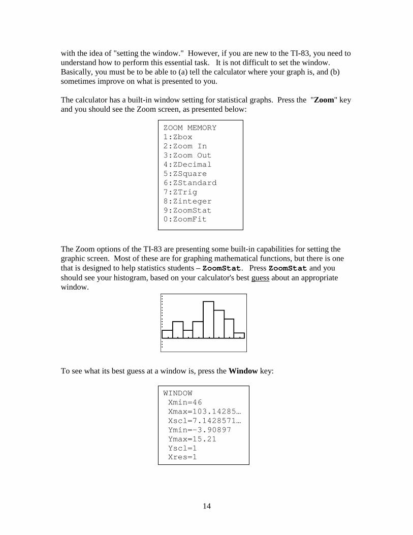
with the idea of "setting the window." However, if you are new to the TI-83, you need to understand how to perform this essential task. It is not difficult to set the window. Basically, you must be to be able to (a) tell the calculator where your graph is, and (b) sometimes improve on what is presented to you. The calculator has a built-in window setting for statistical graphs. Press the "Zoom" key and you should see the Zoom screen, as presented below: The Zoom options of the TI-83 are presenting some built-in capabilities for setting the graphic screen. Most of these are for graphing mathematical functions, but there is one that is designed to help statistics students – ZoomStat. Press ZoomStat and you should see your histogram, based on your calculator's best guess about an appropriate window. To see what its best guess at a window is, press the Window key:

ZOOM MEMORY 1:Zbox 2:Zoom In 3:Zoom Out 4:ZDecimal 5:ZSquare 6:ZStandard 7:ZTrig 8:Zinteger 9:ZoomStat 0:ZoomFit

15

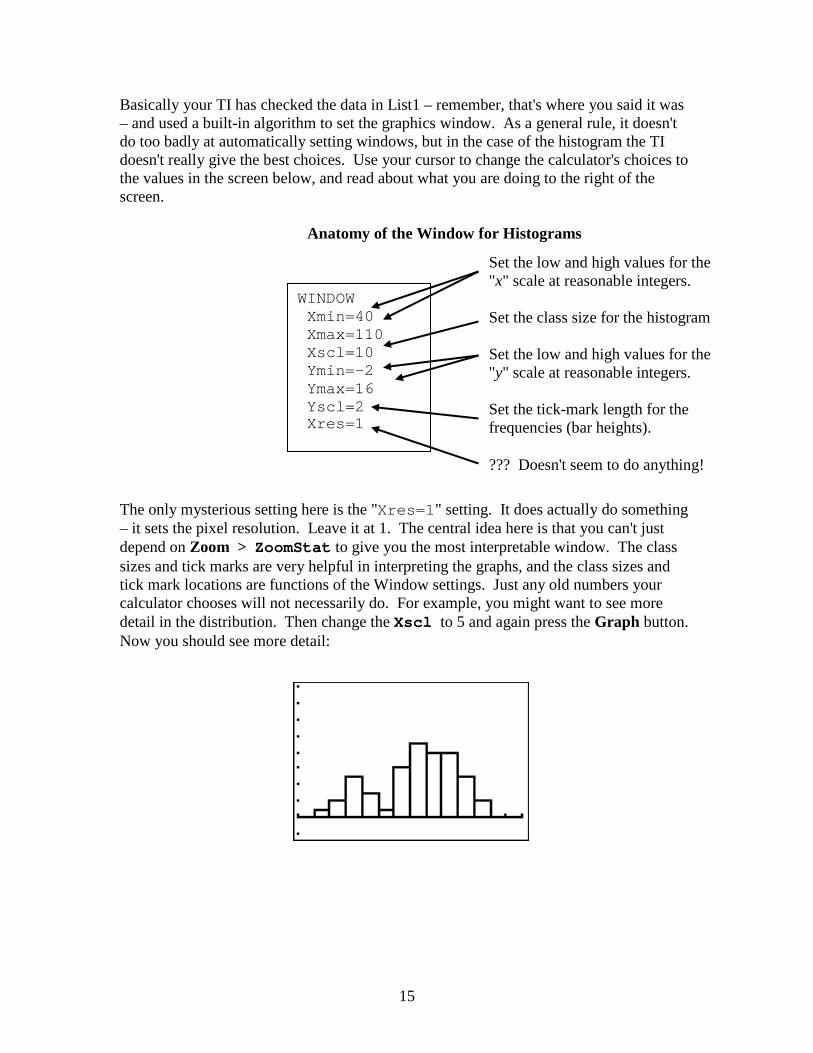
Basically your TI has checked the data in List1 – remember, that's where you said it was – and used a built-in algorithm to set the graphics window. As a general rule, it doesn't do too badly at automatically setting windows, but in the case of the histogram the TI doesn't really give the best choices. Use your cursor to change the calculator's choices to the values in the screen below, and read about what you are doing to the right of the screen. Anatomy of the Window for Histograms The only mysterious setting here is the "Xres=1" setting. It does actually do something – it sets the pixel resolution. Leave it at 1. The central idea here is that you can't just depend on Zoom > ZoomStat to give you the most interpretable window. The class sizes and tick marks are very helpful in interpreting the graphs, and the class sizes and tick mark locations are functions of the Window settings. Just any old numbers your calculator chooses will not necessarily do. For example, you might want to see more detail in the distribution. Then change the Xscl to 5 and again press the Graph button. Now you should see more detail:

WINDOW Xmin=40 Xmax=110 Xscl=10 Ymin=-2 Ymax=16 Yscl=2 Xres=1

Set the low and high values for the "x" scale at reasonable integers. Set the class size for the histogram Set the low and high values for the "y" scale at reasonable integers. Set the tick-mark length for the frequencies (bar heights). ??? Doesn't seem to do anything!

16

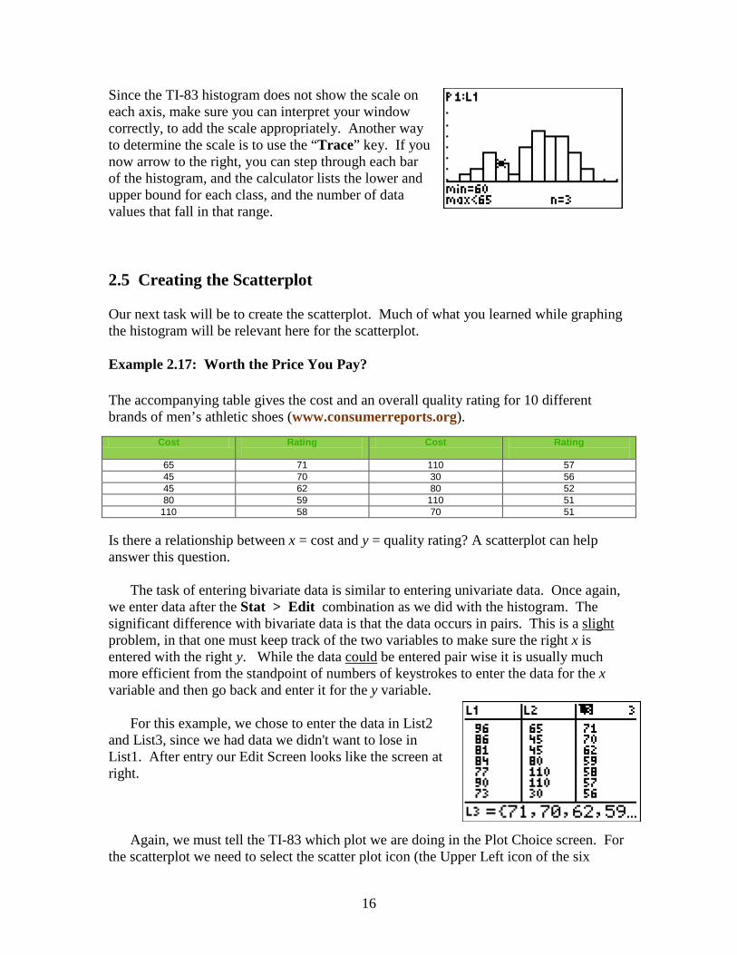
Since the TI-83 histogram does not show the scale on each axis, make sure you can interpret your window correctly, to add the scale appropriately. Another way to determine the scale is to use the “Trace” key. If you now arrow to the right, you can step through each bar of the histogram, and the calculator lists the lower and upper bound for each class, and the number of data values that fall in that range. 2.5 Creating the Scatterplot Our next task will be to create the scatterplot. Much of what you learned while graphing the histogram will be relevant here for the scatterplot. Example 2.17: Worth the Price You Pay? The accompanying table gives the cost and an overall quality rating for 10 different brands of men’s athletic shoes (www.consumerreports.org).

Cost Rating

Cost Rating

65 71 110 57 45 70 30 56 45 62 80 52 80 59 110 51

110 58 70 51 Is there a relationship between x = cost and y = quality rating? A scatterplot can help answer this question.

The task of entering bivariate data is similar to entering univariate data. Once again, we enter data after the Stat > Edit combination as we did with the histogram. The significant difference with bivariate data is that the data occurs in pairs. This is a slight problem, in that one must keep track of the two variables to make sure the right x is entered with the right y. While the data could be entered pair wise it is usually much more efficient from the standpoint of numbers of keystrokes to enter the data for the x variable and then go back and enter it for the y variable.

For this example, we chose to enter the data in List2

and List3, since we had data we didn't want to lose in List1. After entry our Edit Screen looks like the screen at right.

Again, we must tell the TI-83 which plot we are doing in the Plot Choice screen. For

the scatterplot we need to select the scatter plot icon (the Upper Left icon of the six

17

displayed.) Notice that as soon as you do this you must specify two lists: the XList and YList. Since we entered our data in the List2 and List3, these lists will be our choices for the scatterplot. Defining which list is the XList and which is the YList determines which variable will be the horizontal axis variable, and which will be the vertical axis variable. Since our "x" variable is in List2, and "y" variable is in List3, the choices in the Plot Choice screen (2nd > Stat Plot > Plot1…) would be: XList: 2L YList: 3L

We also have another choice at this point, the "Mark" value. The scatter plot is, of course, comprised of dots, and we have some choices as to what we want the dots to look like. Those choices are displayed in the screen by the "Mark:"

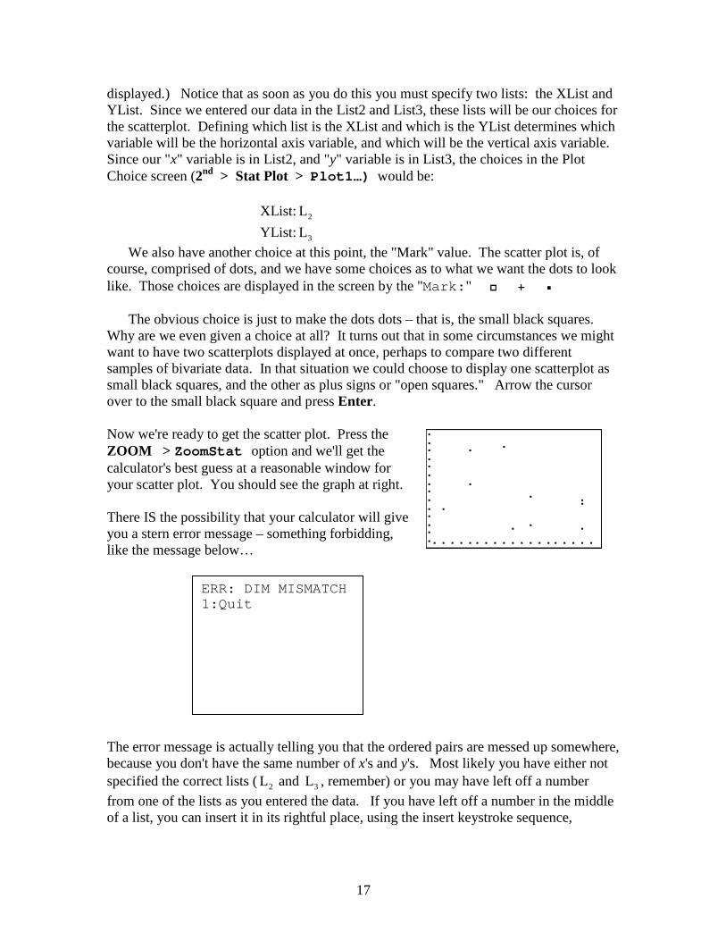
The obvious choice is just to make the dots dots – that is, the small black squares. Why are we even given a choice at all? It turns out that in some circumstances we might want to have two scatterplots displayed at once, perhaps to compare two different samples of bivariate data. In that situation we could choose to display one scatterplot as small black squares, and the other as plus signs or "open squares." Arrow the cursor over to the small black square and press Enter. Now we're ready to get the scatter plot. Press the ZOOM > ZoomStat option and we'll get the calculator's best guess at a reasonable window for your scatter plot. You should see the graph at right. There IS the possibility that your calculator will give you a stern error message – something forbidding, like the message below… The error message is actually telling you that the ordered pairs are messed up somewhere, because you don't have the same number of x's and y's. Most likely you have either not specified the correct lists ( 2L and 3L , remember) or you may have left off a number from one of the lists as you entered the data. If you have left off a number in the middle of a list, you can insert it in its rightful place, using the insert keystroke sequence,

ERR: DIM MISMATCH 1:Quit

18

2nd > INS To use this feature, place the cursor at the right place in the right list where you should have entered the right number. Press the 2nd > INS sequence, and then enter the missing number. At this point we should see the correct scatterplot.

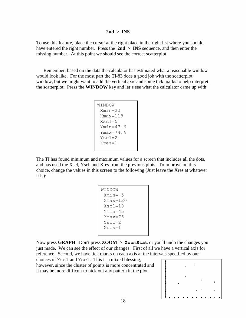
Remember, based on the data the calculator has estimated what a reasonable window would look like. For the most part the TI-83 does a good job with the scatterplot window, but we might want to add the vertical axis and some tick marks to help interpret the scatterplot. Press the WINDOW key and let’s see what the calculator came up with: The TI has found minimum and maximum values for a screen that includes all the dots, and has used the Xscl, Yscl, and Xres from the previous plots. To improve on this choice, change the values in this screen to the following (Just leave the Xres at whatever it is): Now press GRAPH. Don't press ZOOM > ZoomStat or you'll undo the changes you just made. We can see the effect of our changes. First of all we have a vertical axis for reference. Second, we have tick marks on each axis at the intervals specified by our choices of Xscl and Yscl. This is a mixed blessing, however, since the cluster of points is more concentrated and it may be more difficult to pick out any pattern in the plot.

WINDOW Xmin=22 Xmax=118 Xscl=5 Ymin=47.6 Ymax=74.4 Yscl=2 Xres=1

WINDOW Xmin=-5 Xmax=120 Xscl=10 Ymin=45 Ymax=75 Yscl=2 Xres=1

19

In general, these WINDOW choices are a matter of taste and judgment, wisdom guided by experience. 2.6 Conclusion

A great deal of what we did here for producing statistical graphs is merely repeated for future plots. When we make other types of plots, you will already know how to set up the Plot Choice screen, and so all you will really need to know is which icon to use.

20

EDIT CALC TESTS 1:1-Var Stats 2:2-Var Stats 3:Med-Med 4:LinReg(ax+b) 5:QuadReg 6:CubicReg 7:QuartReg 8:LinReg(a+bx) 9:LnReg 0:ExpReg A:PwrReg B:Logistic C:SinReg

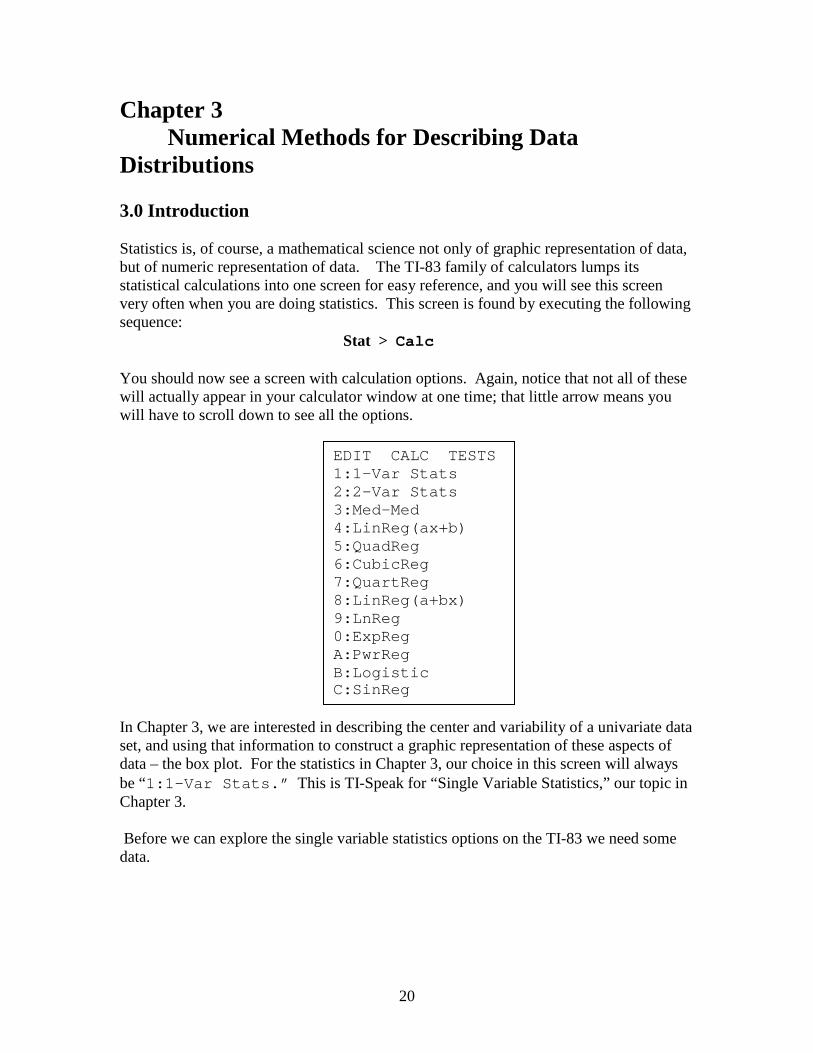
Chapter 3 Numerical Methods for Describing Data Distributions 3.0 Introduction Statistics is, of course, a mathematical science not only of graphic representation of data, but of numeric representation of data. The TI-83 family of calculators lumps its statistical calculations into one screen for easy reference, and you will see this screen very often when you are doing statistics. This screen is found by executing the following sequence: Stat > Calc You should now see a screen with calculation options. Again, notice that not all of these will actually appear in your calculator window at one time; that little arrow means you will have to scroll down to see all the options. In Chapter 3, we are interested in describing the center and variability of a univariate data set, and using that information to construct a graphic representation of these aspects of data – the box plot. For the statistics in Chapter 3, our choice in this screen will always be “1:1-Var Stats.” This is TI-Speak for “Single Variable Statistics,” our topic in Chapter 3. Before we can explore the single variable statistics options on the TI-83 we need some data.

21

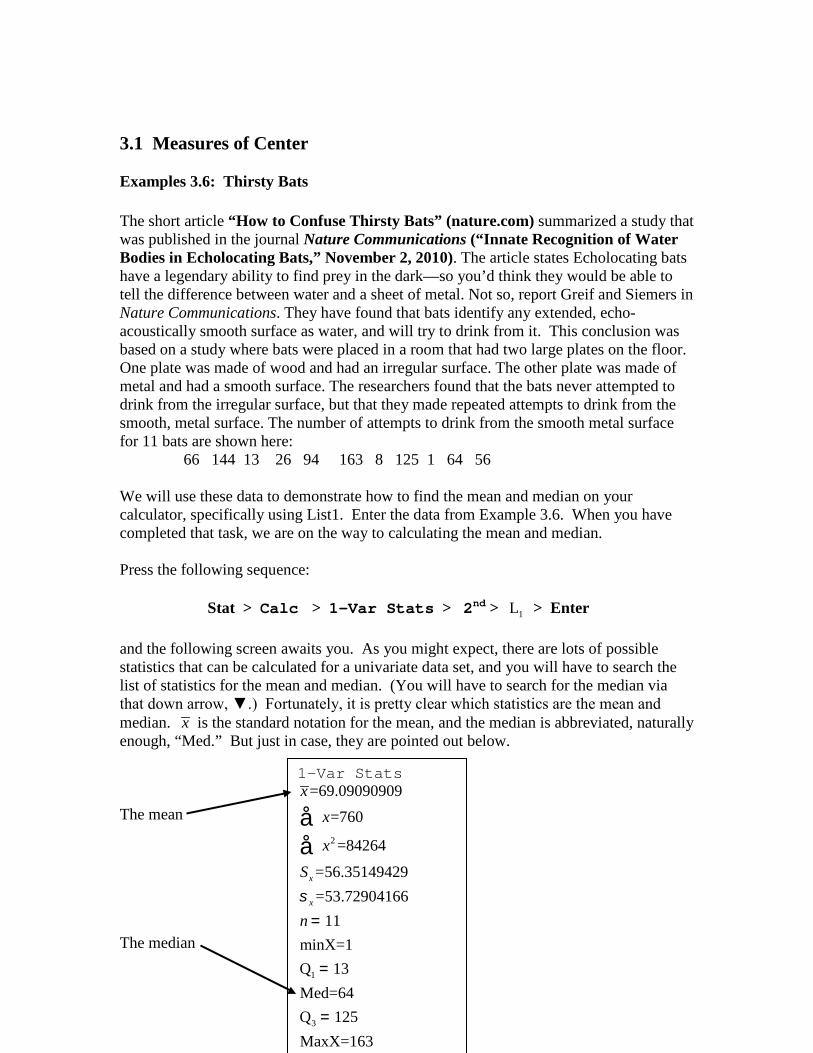
3.1 Measures of Center Examples 3.6: Thirsty Bats The short article “How to Confuse Thirsty Bats” (nature.com) summarized a study that was published in the journal Nature Communications (“Innate Recognition of Water Bodies in Echolocating Bats,” November 2, 2010). The article states Echolocating bats have a legendary ability to find prey in the dark—so you’d think they would be able to tell the difference between water and a sheet of metal. Not so, report Greif and Siemers in Nature Communications. They have found that bats identify any extended, echo-acoustically smooth surface as water, and will try to drink from it. This conclusion was based on a study where bats were placed in a room that had two large plates on the floor. One plate was made of wood and had an irregular surface. The other plate was made of metal and had a smooth surface. The researchers found that the bats never attempted to drink from the irregular surface, but that they made repeated attempts to drink from the smooth, metal surface. The number of attempts to drink from the smooth metal surface for 11 bats are shown here: 66 144 13 26 94 163 8 125 1 64 56 We will use these data to demonstrate how to find the mean and median on your calculator, specifically using List1. Enter the data from Example 3.6. When you have completed that task, we are on the way to calculating the mean and median. Press the following sequence: Stat > Calc > 1-Var Stats > 2nd > 1L > Enter and the following screen awaits you. As you might expect, there are lots of possible statistics that can be calculated for a univariate data set, and you will have to search the list of statistics for the mean and median. (You will have to search for the median via that down arrow, ▼.) Fortunately, it is pretty clear which statistics are the mean and median. x is the standard notation for the mean, and the median is abbreviated, naturally enough, “Med.” But just in case, they are pointed out below. The mean The median

1-Var Stats

2

1

3

=69.09090909=760

=84264

=56.35149429=53.72904166

11minX=1Q 13Med=64Q 125MaxX=163

x

x

xx

x

S

ns

=

=

=

åå

22

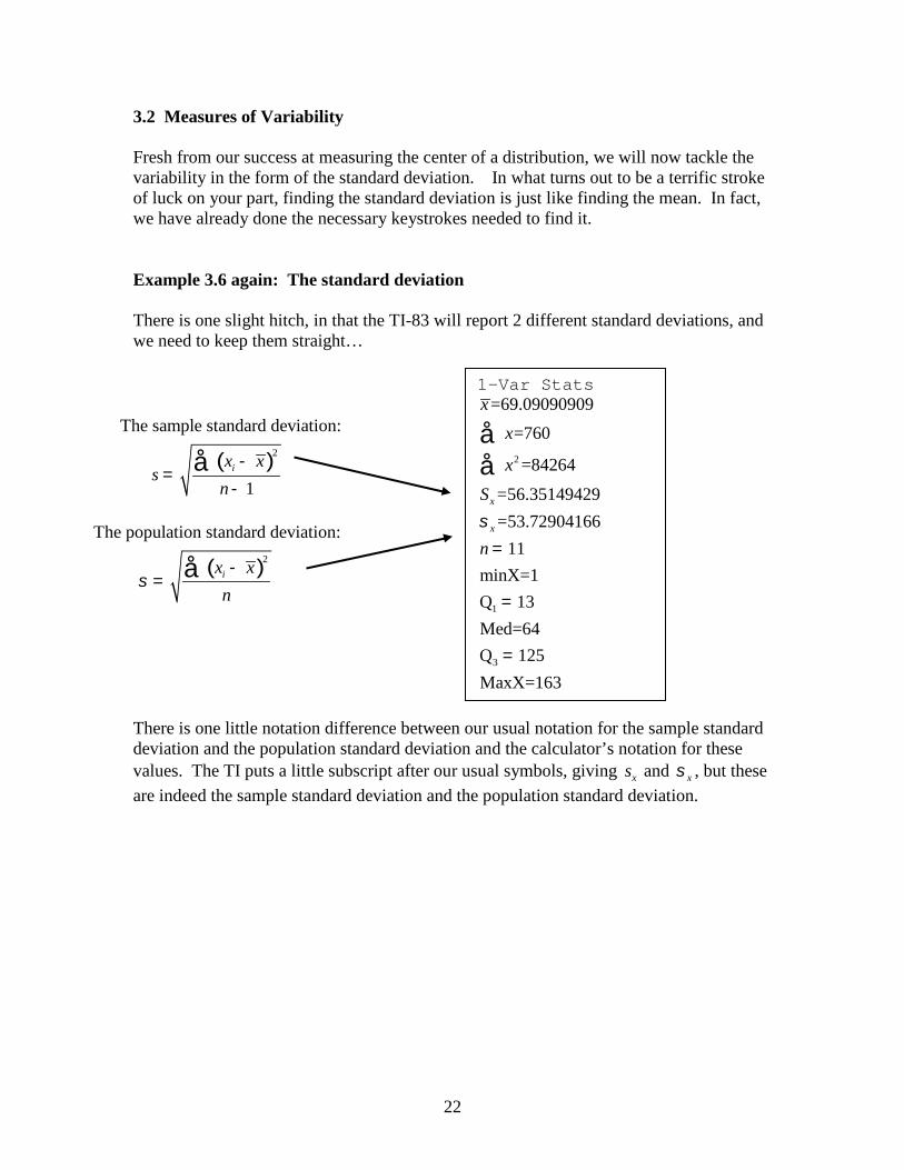
3.2 Measures of Variability Fresh from our success at measuring the center of a distribution, we will now tackle the variability in the form of the standard deviation. In what turns out to be a terrific stroke of luck on your part, finding the standard deviation is just like finding the mean. In fact, we have already done the necessary keystrokes needed to find it. Example 3.6 again: The standard deviation There is one slight hitch, in that the TI-83 will report 2 different standard deviations, and we need to keep them straight… There is one little notation difference between our usual notation for the sample standard deviation and the population standard deviation and the calculator’s notation for these values. The TI puts a little subscript after our usual symbols, giving xs and xs , but these are indeed the sample standard deviation and the population standard deviation.

1-Var Stats

2

1

3

=69.09090909=760

=84264

=56.35149429=53.72904166

11minX=1Q 13Med=64Q 125MaxX=163

x

x

xx

x

S

ns

=

=

=

åå

( )2

The sample standard deviation:

1

ix xs

n-

=-

å

( )2

The population standard deviation:

ix xn

s-

= å

23

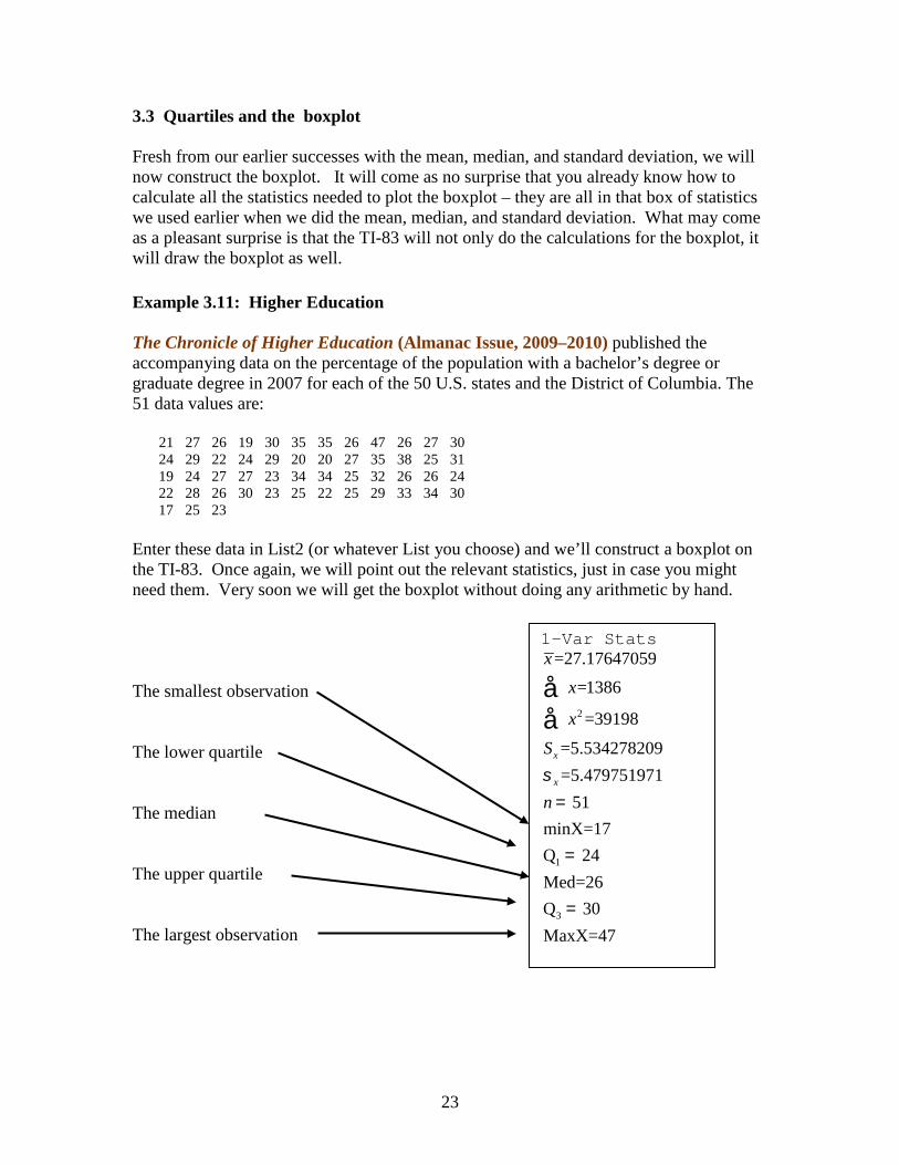
3.3 Quartiles and the boxplot Fresh from our earlier successes with the mean, median, and standard deviation, we will now construct the boxplot. It will come as no surprise that you already know how to calculate all the statistics needed to plot the boxplot – they are all in that box of statistics we used earlier when we did the mean, median, and standard deviation. What may come as a pleasant surprise is that the TI-83 will not only do the calculations for the boxplot, it will draw the boxplot as well. Example 3.11: Higher Education The Chronicle of Higher Education (Almanac Issue, 2009–2010) published the accompanying data on the percentage of the population with a bachelor’s degree or graduate degree in 2007 for each of the 50 U.S. states and the District of Columbia. The 51 data values are:

21 27 26 19 30 35 35 26 47 26 27 30 24 29 22 24 29 20 20 27 35 38 25 31 19 24 27 27 23 34 34 25 32 26 26 24 22 28 26 30 23 25 22 25 29 33 34 30 17 25 23

Enter these data in List2 (or whatever List you choose) and we’ll construct a boxplot on the TI-83. Once again, we will point out the relevant statistics, just in case you might need them. Very soon we will get the boxplot without doing any arithmetic by hand. The smallest observation The lower quartile The median The upper quartile The largest observation

1-Var Stats

2

1

3

=27.17647059=1386

=39198

=5.534278209=5.479751971

51minX=17Q 24Med=26Q 30MaxX=47

x

x

xx

x

S

ns

=

=

=

åå

24

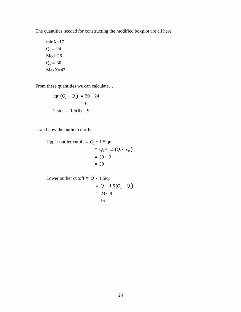
( )3

3 3 1

1

Upper outlier cutoff 1.5iqr 1.5 30 9 39

Lower outlier cutoff 1.5iqr

QQ Q Q

Q

= += + -= +=

= -( )1 3 1 1.5

24 9 16

Q Q Q= - -= -=

The quantities needed for constructing the modified boxplot are all here:

1

3

minX=17Q 24Med=26Q 30MaxX=47

=

=

From these quantities we can calculate…

…and now the outlier cutoffs:

( )3 1iqr 30 24 61.5iqr 1.5(6) 9

Q Q- = -=

= =

25

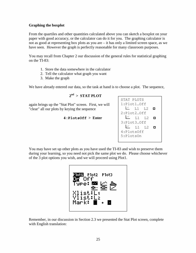
STAT PLOTS 1:Plot1…Off L1 L2 2:Plot2…Off L1 L2 3:Plot3…Off L1 L2 4:PlotsOff 5:PlotsOn

Graphing the boxplot From the quartiles and other quantities calculated above you can sketch a boxplot on your paper with good accuracy, or the calculator can do it for you. The graphing calculator is not as good at representing box plots as you are – it has only a limited screen space, as we have seen. However the graph is perfectly reasonable for many classroom purposes. You may recall from Chapter 2 our discussion of the general rules for statistical graphing on the TI-83: 1. Store the data somewhere in the calculator 2. Tell the calculator what graph you want 3. Make the graph We have already entered our data, so the task at hand is to choose a plot. The sequence, 2nd > STAT PLOT again brings up the "Stat Plot" screen. First, we will "clear" all our plots by keying the sequence 4:PlotsOff > Enter You may have set up other plots as you have used the TI-83 and wish to preserve them during your learning, so you need not pick the same plot we do. Please choose whichever of the 3 plot options you wish, and we will proceed using Plot1. Remember, in our discussion in Section 2.3 we presented the Stat Plot screen, complete with English translation:

26

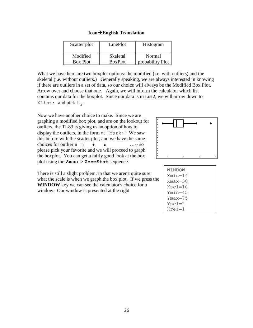
WINDOW Xmin=14 Xmax=50 Xscl=10 Ymin=45 Ymax=75 Yscl=2 Xres=1

IconEnglish Translation

Scatter plot

LinePlot Histogram

Modified Box Plot

Skeletal BoxPlot

Normal probability Plot

What we have here are two boxplot options: the modified (i.e. with outliers) and the skeletal (i.e. without outliers.) Generally speaking, we are always interested in knowing if there are outliers in a set of data, so our choice will always be the Modified Box Plot. Arrow over and choose that one. Again, we will inform the calculator which list contains our data for the boxplot. Since our data is in List2, we will arrow down to XList: and pick 2L . Now we have another choice to make. Since we are graphing a modified box plot, and are on the lookout for outliers, the TI-83 is giving us an option of how to display the outliers, in the form of "Mark:" We saw this before with the scatter plot, and we have the same choices for outlier indicators -- …-- so please pick your favorite and we will proceed to graph the boxplot. You can get a fairly good look at the box plot using the Zoom > ZoomStat sequence. There is still a slight problem, in that we aren't quite sure what the scale is when we graph the box plot. If we press the WINDOW key we can see the calculator's choice for a window. Our window is presented at the right

27

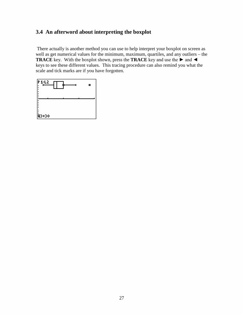
3.4 An afterword about interpreting the boxplot There actually is another method you can use to help interpret your boxplot on screen as well as get numerical values for the minimum, maximum, quartiles, and any outliers – the TRACE key. With the boxplot shown, press the TRACE key and use the ► and ◄ keys to see these different values. This tracing procedure can also remind you what the scale and tick marks are if you have forgotten.

28

Chapter 4 Describing Bivariate Numerical Data 4.0 Introduction In Chapter 4 we address some graphic and numerical descriptions of data when two measures are taken from an individual. In the typical situation we are interested in the question of whether two variables are somehow related, and whether or not the nature of that relationship is linear. That is, can we describe the typical behavior of the variables in the manner of a common algebraic straight line, y mx b= + ? Another description of the data will be numeric – to what extent do our actual data points lie along our straight-line? Our summarizing line is the least squares best fit line, and our numeric description of the degree of "fit" of the line to our data points is Pearson's correlation coefficient. We also assess visually the "goodness" of our fit of the line to the data by considering the residual plot. And the TI-83 will do it all. Let's analyze the data of Example 4.3, the relation between price and quality ratings for bike helmets. 4.1 Pearson's sample correlation coefficient Example 4.3: Does it Pay to Pay More for a Bike Helmet? Are more expensive bike helmets safer than less expensive ones? The accompanying data on x 5 price and y 5 quality rating for 11 different brands of bike helmets is from the Consumer Reports web site (www.consumerreports.org/health). Quality rating was a number from 0 (the worst possible rating) to 100 and was determined using factors that included how well the helmet absorbed the force of an impact, the strength of the helmet, ventilation, and ease of use. We begin, as always, by entering the data after the Stat > Edit sequence. Remember, this data is bivariate so you will have to enter the data in two separate lists. We will use List5 and List6. First, you should analyze your data graphically, by doing the scatterplot (covered in Chapter 2 of this manual). After entering your data in whatever lists you choose, and checking the scatterplot, execute the sequence, Stat > Edit > Calc…

29

EDIT CALC TESTS 1:1-Var Stats 2:2-Var Stats 3:Med-Med 4:LinReg(ax+b) 5:QuadReg 6:CubicReg 7:QuartReg 8:LinReg(a+bx) 9:LnReg 0:ExpReg A:PwrReg B:Logistic C:SinReg

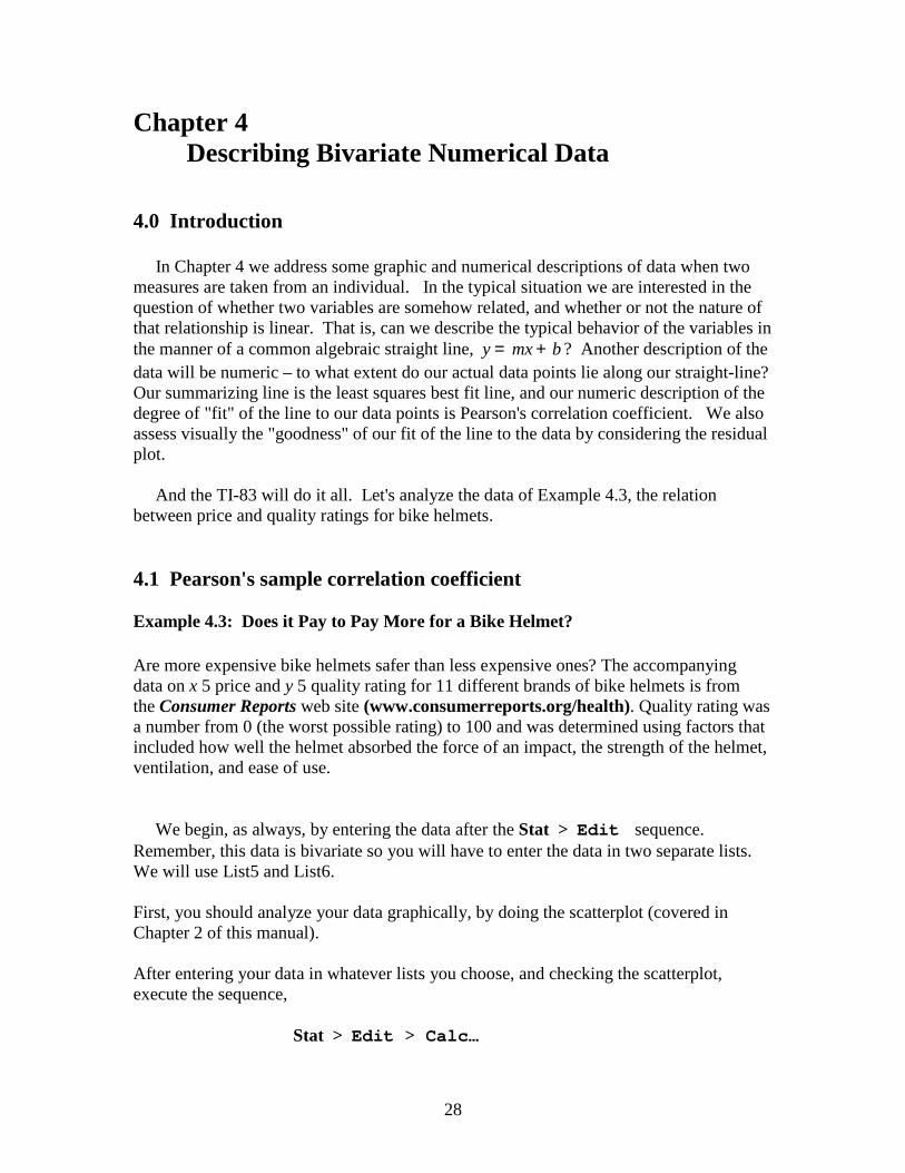
Take a deep breath, and check out these options: One would think one should pick 2:2-Var Stats from the list, and out would pop the Pearson correlation coefficient. Unfortunately, for reasons known only to the TI-83 design engineers, choosing that option gives you all the information you need if you wanted to calculate Pearson's correlation using the formula in Example 4.1 – but doesn't give you the correlation! To get Pearson's r you have to choose a different option, one that is not the most obvious choice. (If you have read Section 4.2 in the text, you will know why this is a reasonable choice, but it still isn't obvious.) The lack of obvious is more than compensated for by the fact that you have two options that are equally adept at presenting the correlation coefficient: 4:LinReg(ax+b) and 8:LinReg(a+bx). Both these options accomplish the same thing, but they use the variables a and b in different roles. In the text the variables are used thus: y a bx= + . It is probably better to use the choice that matches the text, but either way the calculator will give the same numeric values. Now we have some bad news to give you: (a) picking either of these choices will get you information you haven't asked for, and (b) you may not actually get the correlation you are hoping for. But don't lose hope yet. Choose the following sequence: Stat > Calc > 8:LinReg(a+bx) > 5 6L , L > Enter (If your data is anywhere except List1 and List2, you have to tell the TI where they are – hence you need to explicitly add the 5 6L , L .) Here's what we see on our calculator: and then…

8:LinReg(a+bx) 5 6L , L

LinReg y=a+bx a=39.57470349 b=.3122661785

30

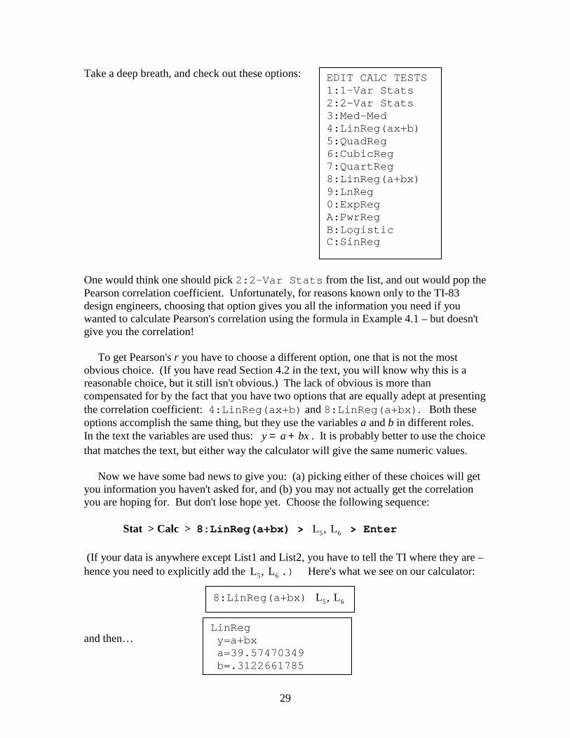
Not only do we have information we didn't ask for, we don't have Pearson's r, which we did ask for. What has gone wrong here is not the extra information; it’s the missing information. For reasons unknown, the TI-83 calculator right out of the box does not present r. Use the following keystroke form: 2nd > CATALOG… Arrow down, down, down, until you get to the D's, and execute this keystroke sequence: DiagnosticOn > Enter > Enter (Yes, press Enter two times) Fortunately this DiagnosticOn set of keystrokes only has to be done once. The DiagnosticOn tells the calculator that Yes, you want to see Pearson's r.

Now let's start at the top… Stat > Calc > 8:LinReg(a+bx) > 5 6L , L > Enter Here's what we see on our calculator at this point: and…

CATALOG ►abs( and angle( ANOVA( Ans (etc.)

8:LinReg(a+bx) 5 6L , L

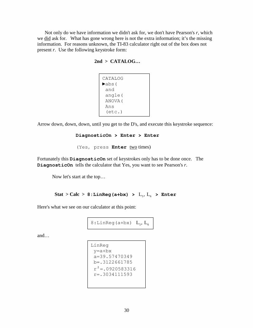
LinReg y=a+bx a=39.57470349 b=.3122661785 r 2 =.0920583316 r=.3034111593

31

We have succeeded in getting Pearson's correlation. 0.303r » . 4.2 The regression line Example 4.6: It May Be a Pile of Debris to You, but It Is Home to a Mouse The accompanying data is a subset of data from a scatterplot that appeared in the paper “Small Mammal Responses to Fine Woody Debris and Forest Fuel Reduction in Southwest Oregon” (Journal of Wildlife Management [2005]: 625–632). The authors of the paper were interested in how the distance a deer mouse will travel for food is related to the distance from the food to the nearest pile of fine woody debris. Distances were measured in meters.

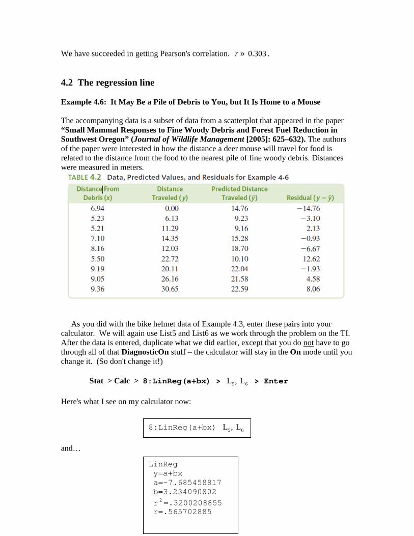
As you did with the bike helmet data of Example 4.3, enter these pairs into your calculator. We will again use List5 and List6 as we work through the problem on the TI. After the data is entered, duplicate what we did earlier, except that you do not have to go through all of that DiagnosticOn stuff – the calculator will stay in the On mode until you change it. (So don't change it!) Stat > Calc > 8:LinReg(a+bx) > 5 6L , L > Enter Here's what I see on my calculator now: and…

8:LinReg(a+bx) 5 6L , L

LinReg y=a+bx a=-7.685458817 b=3.234090802 r 2 =.3200208855 r=.565702885

32

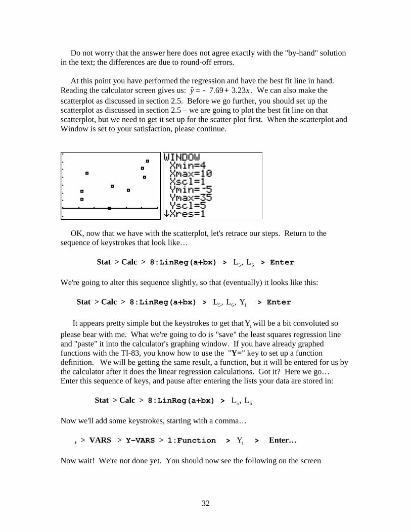
Do not worry that the answer here does not agree exactly with the "by-hand" solution in the text; the differences are due to round-off errors. At this point you have performed the regression and have the best fit line in hand. Reading the calculator screen gives us: ˆ 7.69 3.23y x= - + . We can also make the scatterplot as discussed in section 2.5. Before we go further, you should set up the scatterplot as discussed in section 2.5 – we are going to plot the best fit line on that scatterplot, but we need to get it set up for the scatter plot first. When the scatterplot and Window is set to your satisfaction, please continue.

OK, now that we have with the scatterplot, let's retrace our steps. Return to the sequence of keystrokes that look like… Stat > Calc > 8:LinReg(a+bx) > 5 6L , L > Enter We're going to alter this sequence slightly, so that (eventually) it looks like this: Stat > Calc > 8:LinReg(a+bx) > 5 6 1L , L , Y > Enter

It appears pretty simple but the keystrokes to get that 1Y will be a bit convoluted so please bear with me. What we're going to do is "save" the least squares regression line and "paste" it into the calculator's graphing window. If you have already graphed functions with the TI-83, you know how to use the "Y=" key to set up a function definition. We will be getting the same result, a function, but it will be entered for us by the calculator after it does the linear regression calculations. Got it? Here we go… Enter this sequence of keys, and pause after entering the lists your data are stored in: Stat > Calc > 8:LinReg(a+bx) > 5 6L , L Now we'll add some keystrokes, starting with a comma… , > VARS > Y-VARS > 1:Function > 1Y > Enter… Now wait! We're not done yet. You should now see the following on the screen

33

LinReg y=a+bx a=-7.685458817 b=3.234090802 r 2 =.3200208855 r=.565702885

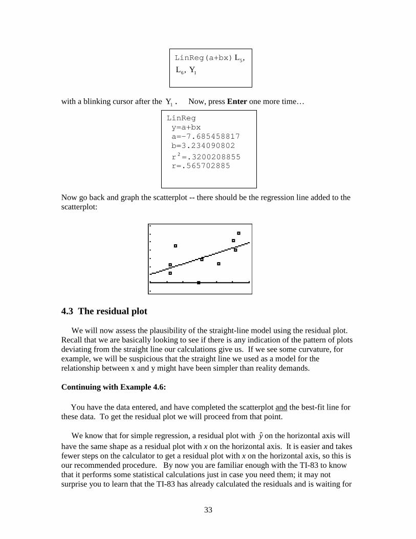
with a blinking cursor after the 1Y . Now, press Enter one more time… Now go back and graph the scatterplot -- there should be the regression line added to the scatterplot: 4.3 The residual plot We will now assess the plausibility of the straight-line model using the residual plot. Recall that we are basically looking to see if there is any indication of the pattern of plots deviating from the straight line our calculations give us. If we see some curvature, for example, we will be suspicious that the straight line we used as a model for the relationship between x and y might have been simpler than reality demands. Continuing with Example 4.6: You have the data entered, and have completed the scatterplot and the best-fit line for these data. To get the residual plot we will proceed from that point. We know that for simple regression, a residual plot with y on the horizontal axis will have the same shape as a residual plot with x on the horizontal axis. It is easier and takes fewer steps on the calculator to get a residual plot with x on the horizontal axis, so this is our recommended procedure. By now you are familiar enough with the TI-83 to know that it performs some statistical calculations just in case you need them; it may not surprise you to learn that the TI-83 has already calculated the residuals and is waiting for

LinReg(a+bx) 5L ,

6 1L , Y

34

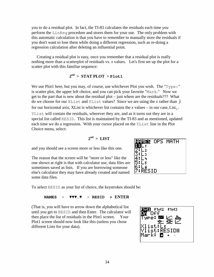
you to do a residual plot. In fact, the TI-83 calculates the residuals each time you perform the LinReg procedure and stores them for your use. The only problem with this automatic calculation is that you have to remember to manually store the residuals if you don't want to lose them while doing a different regression, such as re-doing a regression calculation after deleting an influential point. Creating a residual plot is easy, once you remember that a residual plot is really nothing more than a scatterplot of residuals vs. x values. Let's first set up the plot for a scatter plot with this familiar sequence: 2nd > STAT PLOT > Plot1 We use Plot1 here, but you may, of course, use whichever Plot you wish. The "Type:" is scatter plot, the upper left choice, and you can pick your favorite "Mark." Now we get to the part that is new about the residual plot – just where are the residuals??? What do we choose for our XList and YList values? Since we are using the x rather than y for our horizontal axis, XList is whichever list contains the x values – in our case, 5List . YList will contain the residuals, wherever they are, and as it turns out they are in a special list called RESID. This list is maintained by the TI-83 and as mentioned, updated each time we do a regression. With your cursor placed on the YList line in the Plot Choice menu, select: 2nd > LIST and you should see a screen more or less like this one. The reason that the screen will be "more or less" like the one shown at right is that with calculator use, data files are sometimes saved as lists. If you are borrowing someone else's calculator they may have already created and named some data files. To select RESID as your list of choice, the keystrokes should be: NAMES > ▼▼▼…▼ > RESID > ENTER (That is, you will have to arrow down the alphabetical list until you get to RESID and then Enter. The calculator will then place the list of residuals in the Plot1 screen. Your Plot1 screen should now look like this (unless you chose different Lists for your data).

35

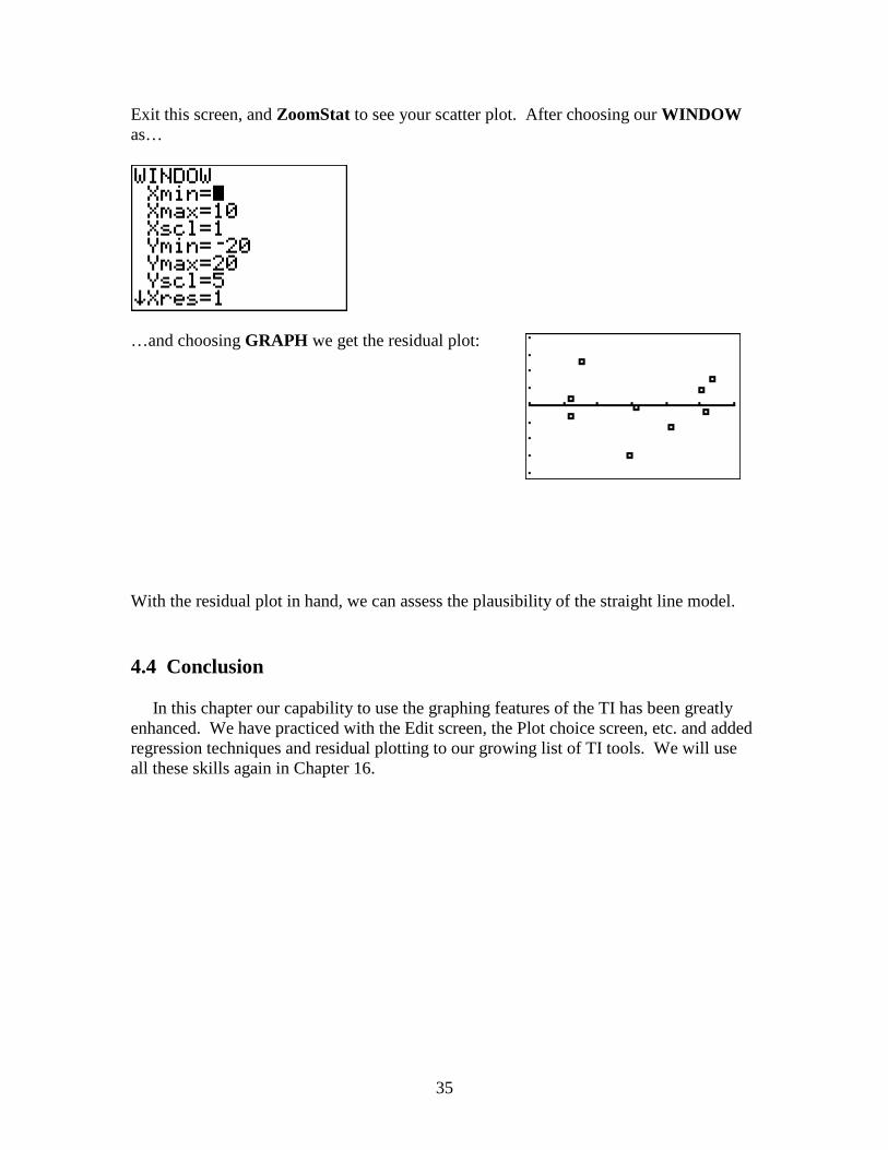
Exit this screen, and ZoomStat to see your scatter plot. After choosing our WINDOW as…

…and choosing GRAPH we get the residual plot: With the residual plot in hand, we can assess the plausibility of the straight line model. 4.4 Conclusion In this chapter our capability to use the graphing features of the TI has been greatly enhanced. We have practiced with the Edit screen, the Plot choice screen, etc. and added regression techniques and residual plotting to our growing list of TI tools. We will use all these skills again in Chapter 16.

36

Chapter 5 Probability 5.0 Introduction In chapter 5 we discover that from the standpoint of arithmetic, probability calculations are fairly routine and the TI-83 performs those calculations without so much as a yawn. Where the TI-83 is a quite helpful is with elementary simulations. (For complicated simulations, one needs a combination of computer and computer programmer.) The TI-83 has built-in functions that generate random numbers and more particularly random numbers that fit certain common statistical situations. If you have even a bit of computer programming experience, you will be able to write programs to do simulations beyond the elementary. Our short introduction here will not require programming, only a few as yet unused keystrokes. Our example for discussion will be the family planning example. 5.1 Simulation Example 5.21: One-Boy Family Planning To help you recall the family planning example, here is a short synopsis:

Suppose that couples who wanted children were to continue having children until a boy is born. Assuming that each newborn child is equally likely to be a boy or a girl, would this behavior change the proportion of boys in the population? We will use simulation to estimate the long-run proportion of boys in the population if families were to continue to have children until they have a boy. This proportion is an estimate of the probability that a randomly selected child from this population is a boy. Note that every sibling group would have exactly one boy.

We will use a single-digit random number to represent a child. The odd digits (1, 3, 5, 7, 9) will represent a male birth, and the even digits will represent a female birth. An observation will be constructed by selecting a sequence of random digits. If the first random number obtained is odd (a boy), the observation is complete. If the first selected number is even (a girl), another digit will be chosen. We continue in this way until an odd digit is obtained. We will use the TI-83 in place of the random number table, but keep the same symbols for the outcomes – odd digits will represent a male birth, even digits a female birth.

37

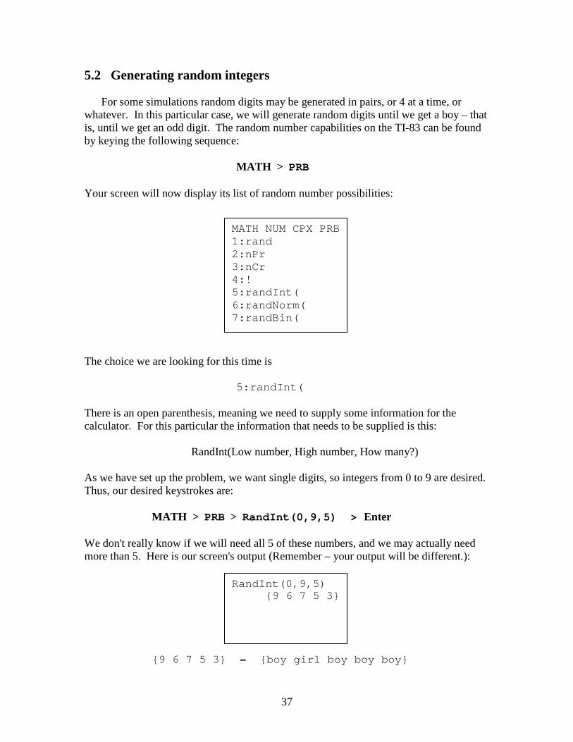
5.2 Generating random integers For some simulations random digits may be generated in pairs, or 4 at a time, or whatever. In this particular case, we will generate random digits until we get a boy – that is, until we get an odd digit. The random number capabilities on the TI-83 can be found by keying the following sequence: MATH > PRB Your screen will now display its list of random number possibilities: The choice we are looking for this time is 5:randInt( There is an open parenthesis, meaning we need to supply some information for the calculator. For this particular the information that needs to be supplied is this: RandInt(Low number, High number, How many?) As we have set up the problem, we want single digits, so integers from 0 to 9 are desired. Thus, our desired keystrokes are: MATH > PRB > RandInt(0,9,5) > Enter We don't really know if we will need all 5 of these numbers, and we may actually need more than 5. Here is our screen's output (Remember – your output will be different.):

{9 6 7 5 3} = {boy girl boy boy boy}

MATH NUM CPX PRB 1:rand 2:nPr 3:nCr 4:! 5:randInt( 6:randNorm( 7:randBin(

RandInt(0,9,5) {9 6 7 5 3}

38

We got a boy with our first try. Of course this wouldn't happen all the time – let's generate some more trials. From where you are now on the screen, press Enter a few times: Enter > Enter > Enter Sibling group 1: {9 6 7 5 3} = { boy girl boy boy boy} Sibling group 2: {2 6 8 1 4} = {girl girl girl boy girl} Sibling group 3: {4 2 8 9 4} = {girl girl girl boy girl} Sibling group 4: {4 2 6 6 8} = {girl girl girl girl girl} No boy yet in that sibling group 4. We'll have to simulate some more births: Enter Sibling group 4 (Cont'd): {7 4 9 6 3} = { boy girl boy girl boy} Since we only needed to get 1 boy, our trial stops after the first new birth. After simulating four sibling groups, we have 4 boys among 15 children. The proportion of boys is 4/19, which is not yet close to the theoretical probability of 0.5. However, continuing the simulation to obtain a large number of observations would be consistent with a probability of half the population being boys under this family planning method. 5.3 Afterword We have only scratched the surface of the simulation possibilities for the TI-83 here. Consult your manual to see what some of those other options for random numbers can do, and try some more complicated simulations. They're actually fun!

RandInt(0,9,5) {9 6 7 5 3} {2 6 8 1 4} {4 2 8 9 4} {4 2 6 6 8}

39

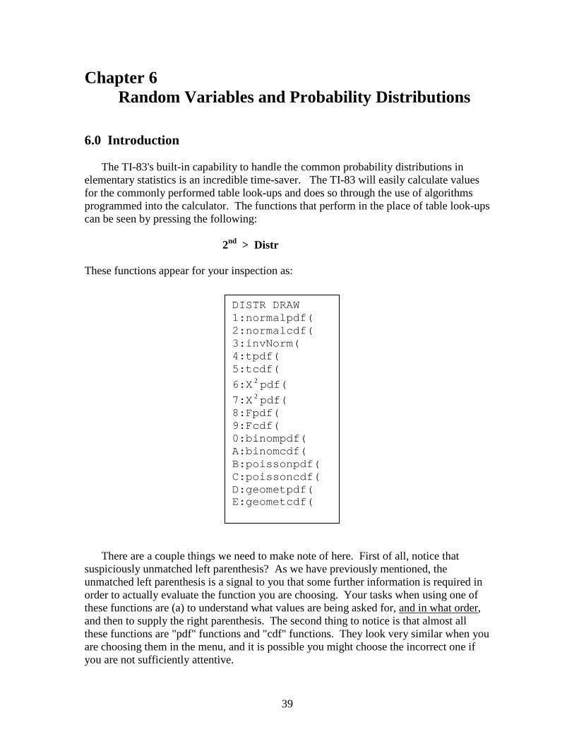
Chapter 6 Random Variables and Probability Distributions 6.0 Introduction The TI-83's built-in capability to handle the common probability distributions in elementary statistics is an incredible time-saver. The TI-83 will easily calculate values for the commonly performed table look-ups and does so through the use of algorithms programmed into the calculator. The functions that perform in the place of table look-ups can be seen by pressing the following: 2nd > Distr These functions appear for your inspection as:

There are a couple things we need to make note of here. First of all, notice that suspiciously unmatched left parenthesis? As we have previously mentioned, the unmatched left parenthesis is a signal to you that some further information is required in order to actually evaluate the function you are choosing. Your tasks when using one of these functions are (a) to understand what values are being asked for, and in what order, and then to supply the right parenthesis. The second thing to notice is that almost all these functions are "pdf" functions and "cdf" functions. They look very similar when you are choosing them in the menu, and it is possible you might choose the incorrect one if you are not sufficiently attentive.

DISTR DRAW 1:normalpdf( 2:normalcdf( 3:invNorm( 4:tpdf( 5:tcdf( 6:X 2 pdf( 7:X 2 pdf( 8:Fpdf( 9:Fcdf( 0:binompdf( A:binomcdf( B:poissonpdf( C:poissoncdf( D:geometpdf( E:geometcdf(

40

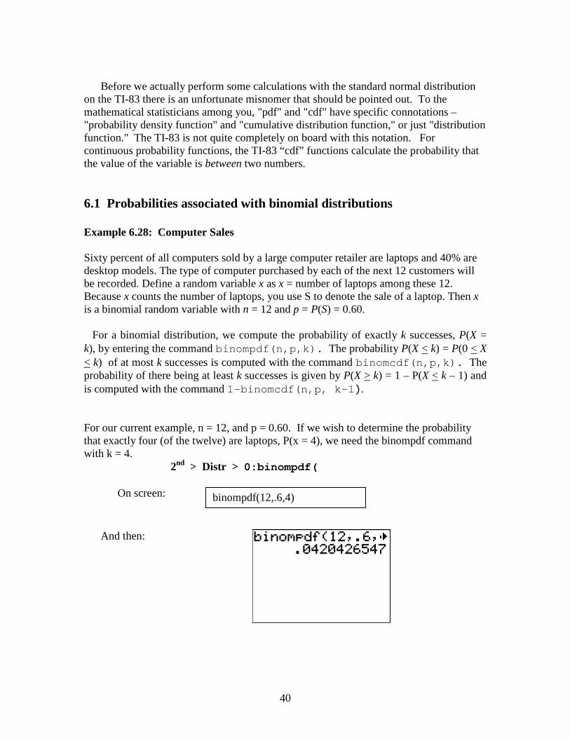
Before we actually perform some calculations with the standard normal distribution on the TI-83 there is an unfortunate misnomer that should be pointed out. To the mathematical statisticians among you, "pdf" and "cdf" have specific connotations – "probability density function" and "cumulative distribution function," or just "distribution function." The TI-83 is not quite completely on board with this notation. For continuous probability functions, the TI-83 “cdf” functions calculate the probability that the value of the variable is between two numbers. 6.1 Probabilities associated with binomial distributions Example 6.28: Computer Sales Sixty percent of all computers sold by a large computer retailer are laptops and 40% are desktop models. The type of computer purchased by each of the next 12 customers will be recorded. Define a random variable x as x = number of laptops among these 12. Because x counts the number of laptops, you use S to denote the sale of a laptop. Then x is a binomial random variable with n = 12 and p = P(S) = 0.60. For a binomial distribution, we compute the probability of exactly k successes, P(X = k), by entering the command binompdf(n,p,k). The probability P(X < k) = P(0 < X < k) of at most k successes is computed with the command binomcdf(n,p,k). The probability of there being at least k successes is given by P(X > k) = 1 – P(X < k – 1) and is computed with the command 1–binomcdf(n,p, k–1). For our current example, n = 12, and p = 0.60. If we wish to determine the probability that exactly four (of the twelve) are laptops, P(x = 4), we need the binompdf command with k = 4. 2nd > Distr > 0:binompdf( On screen: And then:

binompdf(12,.6,4)

41

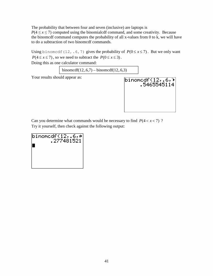
binomcdf(12,.6,7) – binomcdf(12,.6,3)

The probability that between four and seven (inclusive) are laptops is P(4 ≤ x ≤ 7) computed using the binomialcdf command, and some creativity. Because the binomcdf command computes the probability of all x-values from 0 to k, we will have to do a subtraction of two binomcdf commands. Using binomcdf(12,.6,7) gives the probability of (0 7)P x≤ ≤ . But we only want

(4 7)P x≤ ≤ , so we need to subtract the (0 3)P x≤ ≤ . Doing this as one calculator command: Your results should appear as: Can you determine what commands would be necessary to find (4 7)P x< < ? Try it yourself, then check against the following output:

42

6.2 Probabilities associated with normal distributions Example 6.21: Newborn Birth Weights Problem #1: ( )P a x b< < Data from the paper “Fetal Growth Parameters and Birth Weight: Their Relationship to Neonatal Body Composition” (Ultrasound in Obstetrics and Gynecology [2009]: 441–446) suggest that a normal distribution with mean 3500µ = grams and standard deviation s = 600 grams is a reasonable model for the probability distribution of x = birth weight of a randomly selected full-term baby. What proportion of birth weights are between 2,900 and 4,700 grams? To answer this question, you must find P(2,900 < x < 4,700). Because the normal curve we are investigating is not the standard normal curve – and thus does not match the Normal Curve Tables – we have to do a little preliminary work. Translating to an equivalent problem for the standard normal distribution,

2900 3500* 1.00600

4700 3500* 2.00600

aa

bb

µσµ

σ

− −= = = −

− −= = =

Then

(2900 4700) ( 1.00 2.00)( curve area to the left of 2.00) ( curve area to the left of -1.00).9772 .1587.8185

P x P zz z

< < = − < <= −= −=

The TI-83 can take the place of this table lookup and save a great deal of time. The function we will use to find the area between z = -1.00 and 2.00 for the standard normal distribution is the "normalcdf" function. Here's the sequence: 2nd > DISTR > normalcdf( Now we are a bit worried. We know – because of that left parenthesis – that we are supposed to supply some information, and that the order we enter it is important. A brief referral to the TI-83 manual tells us the order: normalcdf (lower bound, upper bound [ , µ, σ] )

43

On the TI-83 you must supply the lower bound and upper bound with the appropriate values for z, and the mean and standard deviation. The square brackets, [ ] tell us the mean and standard deviation are options. In the case of the standard normal distribution, we don't need to fill in those options – we will return to them later. At this point, continue the keystroke entry we began earlier:

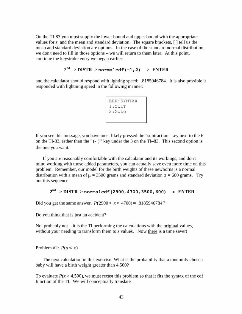
2nd > DISTR > normalcdf(-1,2) > ENTER and the calculator should respond with lighting speed: .8185946784. It is also possible it responded with lightning speed in the following manner: If you see this message, you have most likely pressed the "subtraction" key next to the 6 on the TI-83, rather than the " ( )- " key under the 3 on the TI–83. This second option is the one you want. If you are reasonably comfortable with the calculator and its workings, and don't mind working with those added parameters, you can actually save even more time on this problem. Remember, our model for the birth weights of these newborns is a normal distribution with a mean of µ = 3500 grams and standard deviation σ = 600 grams. Try out this sequence:

2nd > DISTR > normalcdf(2900,4700,3500,600) > ENTER Did you get the same answer, (2900 4700) .8185946784P x< < = ? Do you think that is just an accident? No, probably not – it is the TI performing the calculations with the original values, without your needing to transform them to z values. Now there is a time saver! Problem #2: ( )P a x< The next calculation in this exercise: What is the probability that a randomly chosen baby will have a birth weight greater than 4,500? To evaluate P(x > 4,500), we must recast this problem so that it fits the syntax of the cdf function of the TI. We will conceptually translate

ERR:SYNTAX 1:QUIT 2:Goto

44

( )P a x< into ( )P a x b< < , and think of b as a "very large" number. Just how large a very large number is will depend on the particular normal distribution, but our knowledge of the normal distribution suggests that 10 standard deviations above the mean should be "large enough" so that we haven't missed too much of the probability in the right tail. So let's try this:

2nd > DISTR > normalcdf(4500,3500+10*600,3500,600) > ENTER We are telling the calculator to find the probability of getting a value… 1. 4500,3500+10*600 "between 4500 and 10 standard deviations above the mean, 2. 3500,600 "in a distribution with a mean of 3500 and standard deviation of 600.

And the TI delivers once again! (4500 ) 0.0477903304 0.0478P x< = » . 6.3 Conclusion As can be seen, these probability distribution calculations can be terrific time savers. Just be careful to choose the right function, "pdf" or "cdf", and if you don't want to standardize the distribution to the standard normal, be sure to use those optional parameters carefully.

45

EDIT CALC TESTS 1:Z-Test… 2:T-Test… 3:2-SampZTest… 4:2-SampTTest… 5:1-PropZTest… 6:2-PropZTest… 7:ZInterval… 8:T-Interval… 9:2-SampZInt… 0:2-SampTInt… A:1-PropZInt… B:2-PropZInt… C:X 2 -Test… D:2-SampFTest… E:LinRegTTest… F:ANOVA(

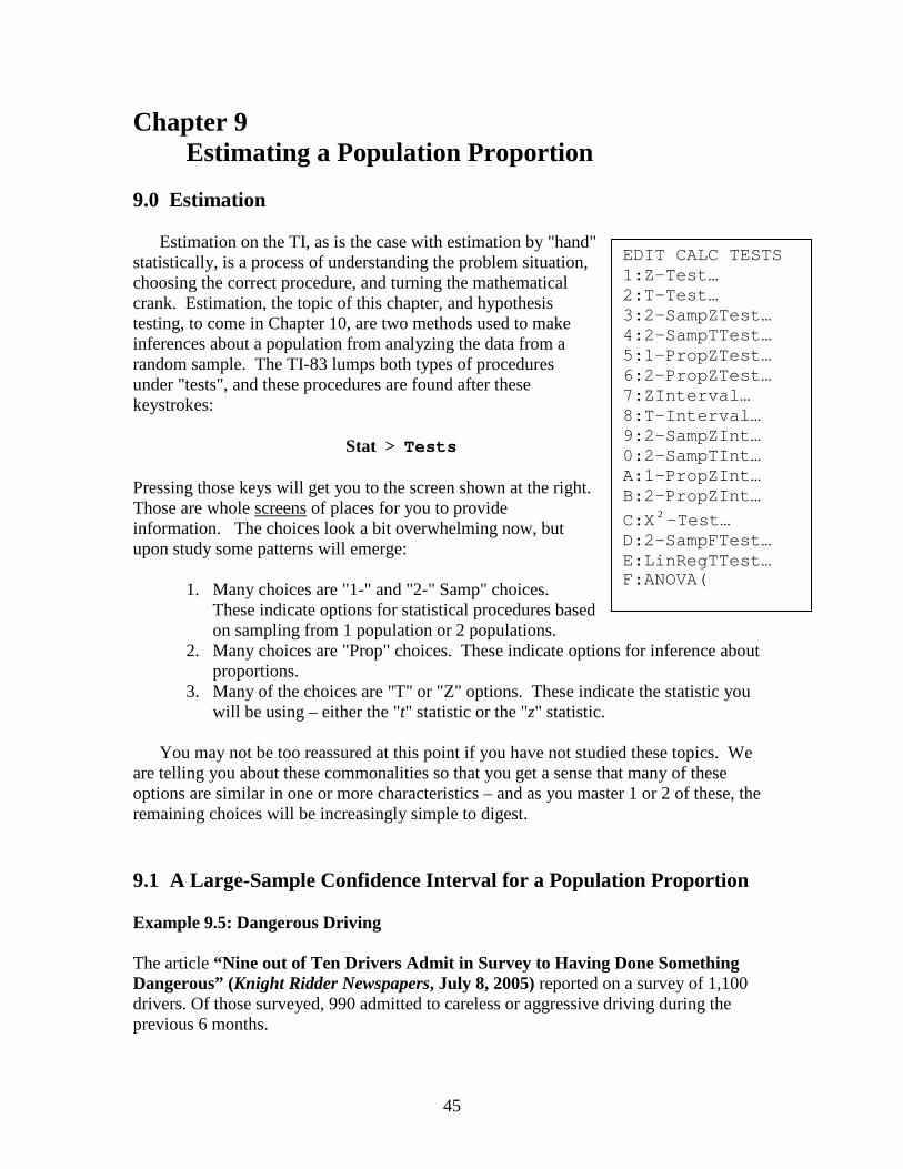
Chapter 9 Estimating a Population Proportion 9.0 Estimation Estimation on the TI, as is the case with estimation by "hand" statistically, is a process of understanding the problem situation, choosing the correct procedure, and turning the mathematical crank. Estimation, the topic of this chapter, and hypothesis testing, to come in Chapter 10, are two methods used to make inferences about a population from analyzing the data from a random sample. The TI-83 lumps both types of procedures under "tests", and these procedures are found after these keystrokes: Stat > Tests Pressing those keys will get you to the screen shown at the right. Those are whole screens of places for you to provide information. The choices look a bit overwhelming now, but upon study some patterns will emerge:

1. Many choices are "1-" and "2-" Samp" choices. These indicate options for statistical procedures based on sampling from 1 population or 2 populations.

2. Many choices are "Prop" choices. These indicate options for inference about proportions.

3. Many of the choices are "T" or "Z" options. These indicate the statistic you will be using – either the "t" statistic or the "z" statistic.

You may not be too reassured at this point if you have not studied these topics. We

are telling you about these commonalities so that you get a sense that many of these options are similar in one or more characteristics – and as you master 1 or 2 of these, the remaining choices will be increasingly simple to digest. 9.1 A Large-Sample Confidence Interval for a Population Proportion Example 9.5: Dangerous Driving The article “Nine out of Ten Drivers Admit in Survey to Having Done Something Dangerous” (Knight Ridder Newspapers, July 8, 2005) reported on a survey of 1,100 drivers. Of those surveyed, 990 admitted to careless or aggressive driving during the previous 6 months.

46

1-PropZInt x:0 n:0 C-Level: .95 Calculate

Assuming that it is reasonable to regard this sample of 1,100 as representative of the population of drivers, you can use this information to construct an estimate of p, the proportion of all drivers who have engaged in careless or aggressive driving in the last 6 months.

990 .91100

p = =

Since 1100(.9) 990n p = = and µ( )1 1100(.1) 110n p- = = are both greater than or equal

to 10, the sample size is large enough to use the formula for a large-sample confidence interval. A 90% confidence interval for p is then

(1 ) (.9)(.1)( critical value) .90 1.6451100

.90 (1.645)(.009)

.90 .015(.885,0.915)

p pp zn−

± = ±

= ±= ±=

Based on this sample data, we can be 90% confident that the true proportion of drivers who engaged in careless or aggressive driving is between .885 and .915. We have used a method to construct this interval estimate that has a 10% error rate. Up front we need to remind you that checking the assumptions is a critical part of the estimation procedure. Then we need to inform you that the TI-83 does not check these – it's your responsibility as the data analyst to do so. After checking necessary conditions, finding the 90% confidence interval on the TI is a matter of just a few keystrokes… Stat > Tests > … Now we are looking in that huge list for something that suggests a single sample, an interval to estimate a proportion, and a z-statistic.

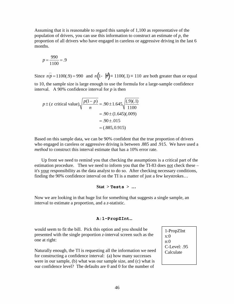
A:1-PropZInt… would seem to fit the bill. Pick this option and you should be presented with the single proportion z-interval screen such as the one at right: Naturally enough, the TI is requesting all the information we need for constructing a confidence interval: (a) how many successes were in our sample, (b) what was our sample size, and (c) what is our confidence level? The defaults are 0 and 0 for the number of

47

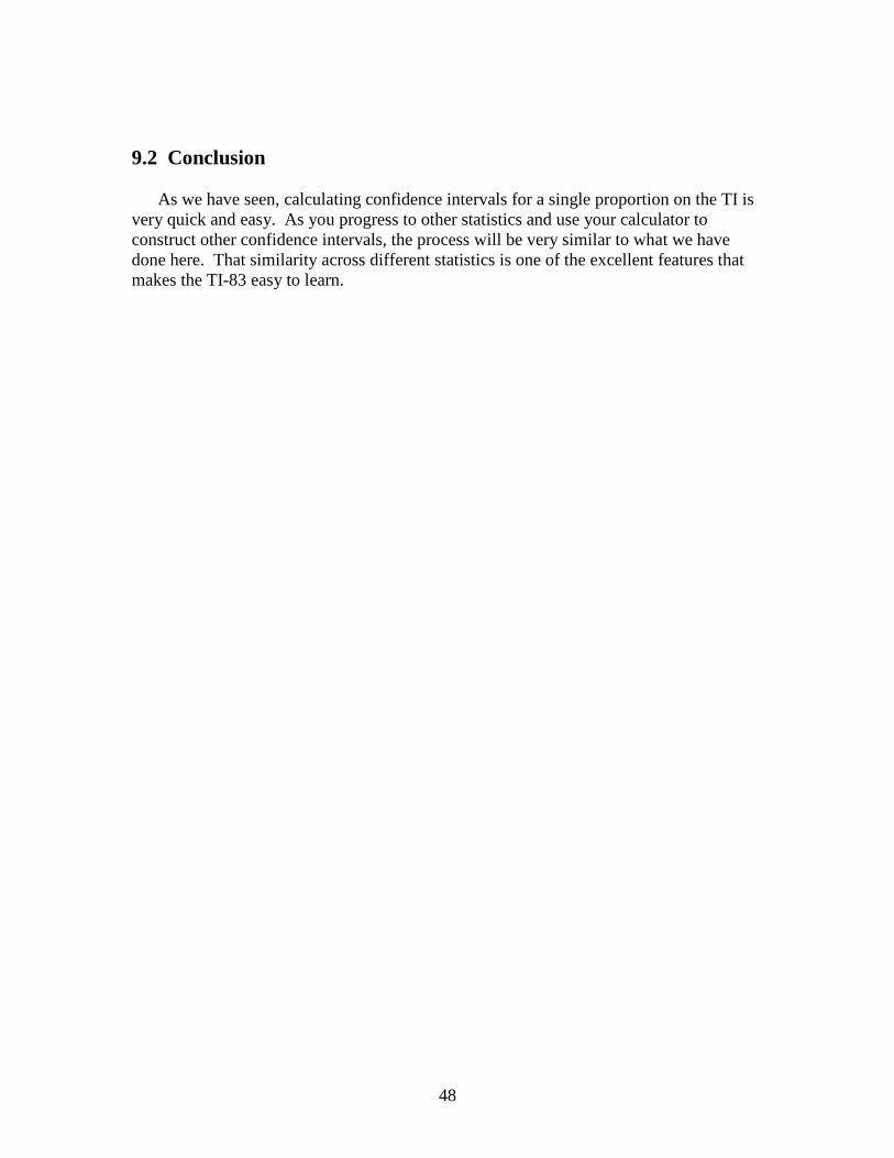
1-PropZInt (.88512,.91488) ˆ .9p = n=1100

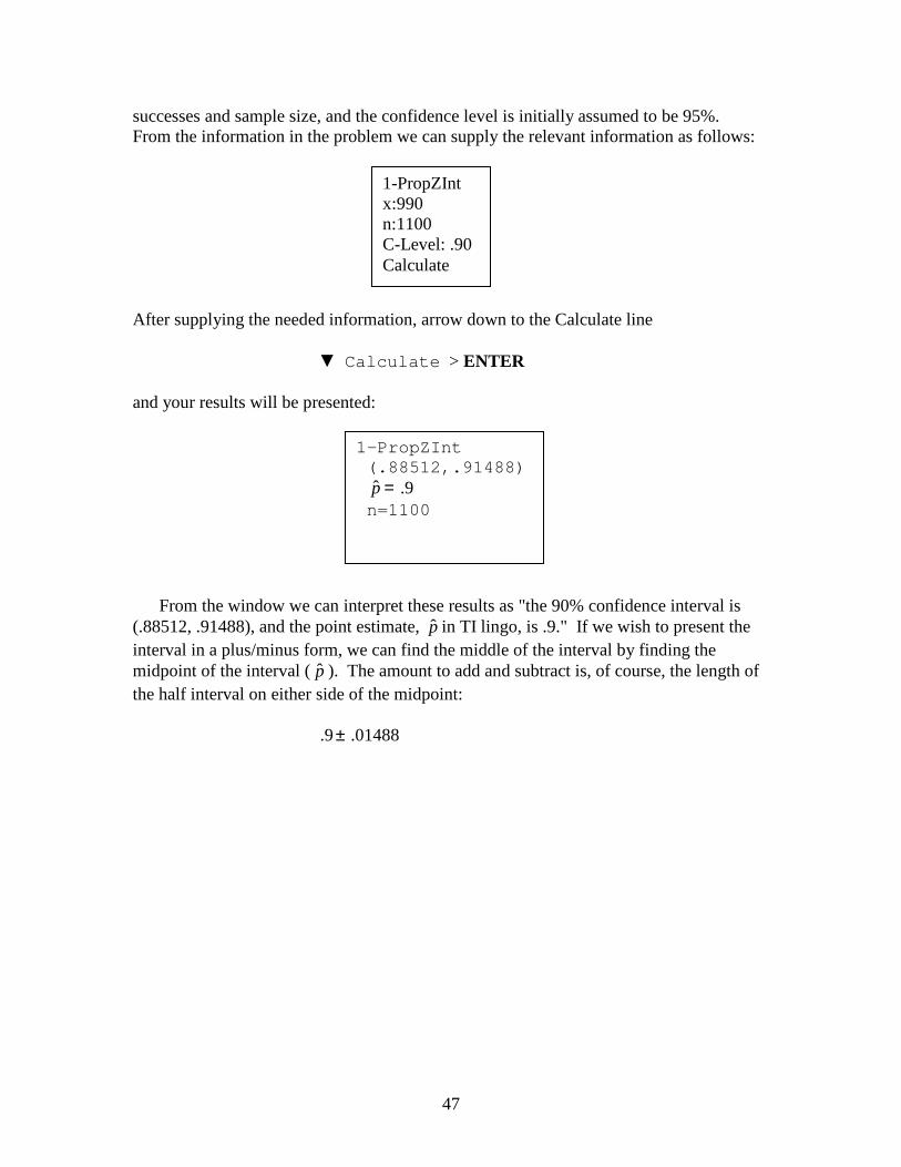
successes and sample size, and the confidence level is initially assumed to be 95%. From the information in the problem we can supply the relevant information as follows: After supplying the needed information, arrow down to the Calculate line ▼ Calculate > ENTER and your results will be presented:

From the window we can interpret these results as "the 90% confidence interval is (.88512, .91488), and the point estimate, p in TI lingo, is .9." If we wish to present the interval in a plus/minus form, we can find the middle of the interval by finding the midpoint of the interval ( p ). The amount to add and subtract is, of course, the length of the half interval on either side of the midpoint: .9 .01488±

1-PropZInt x:990 n:1100 C-Level: .90 Calculate

48

9.2 Conclusion As we have seen, calculating confidence intervals for a single proportion on the TI is very quick and easy. As you progress to other statistics and use your calculator to construct other confidence intervals, the process will be very similar to what we have done here. That similarity across different statistics is one of the excellent features that makes the TI-83 easy to learn.

49

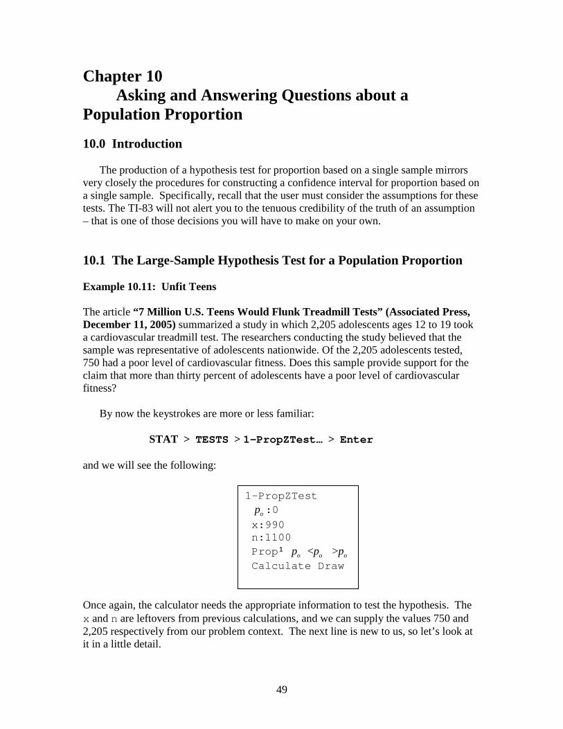
Chapter 10 Asking and Answering Questions about a Population Proportion 10.0 Introduction The production of a hypothesis test for proportion based on a single sample mirrors very closely the procedures for constructing a confidence interval for proportion based on a single sample. Specifically, recall that the user must consider the assumptions for these tests. The TI-83 will not alert you to the tenuous credibility of the truth of an assumption – that is one of those decisions you will have to make on your own. 10.1 The Large-Sample Hypothesis Test for a Population Proportion Example 10.11: Unfit Teens The article “7 Million U.S. Teens Would Flunk Treadmill Tests” (Associated Press, December 11, 2005) summarized a study in which 2,205 adolescents ages 12 to 19 took a cardiovascular treadmill test. The researchers conducting the study believed that the sample was representative of adolescents nationwide. Of the 2,205 adolescents tested, 750 had a poor level of cardiovascular fitness. Does this sample provide support for the claim that more than thirty percent of adolescents have a poor level of cardiovascular fitness? By now the keystrokes are more or less familiar: STAT > TESTS > 1-PropZTest… > Enter and we will see the following: Once again, the calculator needs the appropriate information to test the hypothesis. The x and n are leftovers from previous calculations, and we can supply the values 750 and 2,205 respectively from our problem context. The next line is new to us, so let’s look at it in a little detail.

1-PropZTest op :0 x:990 n:1100 Prop < >o o op p p¹ Calculate Draw

50

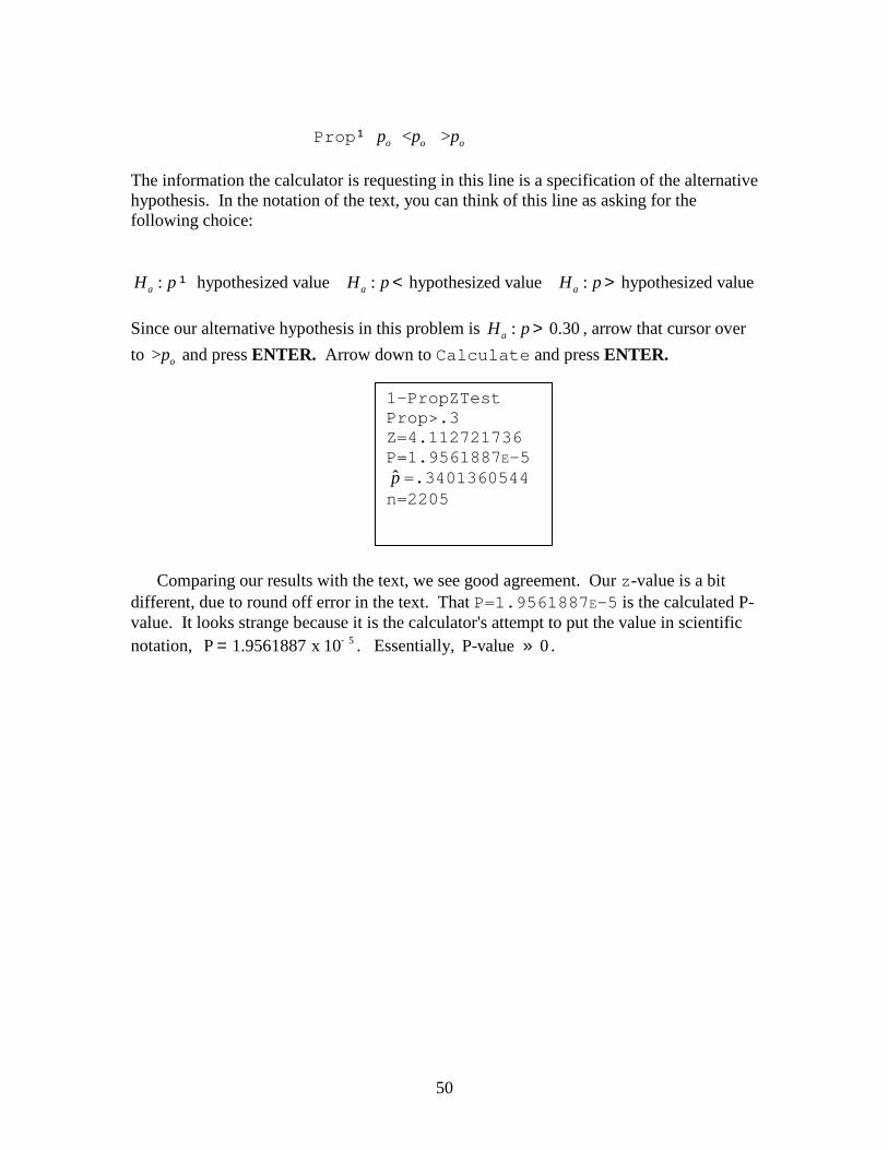
Prop < >o o op p p¹ The information the calculator is requesting in this line is a specification of the alternative hypothesis. In the notation of the text, you can think of this line as asking for the following choice:

: hypothesized value : hypothesized value : hypothesized valuea a aH p H p H p¹ < > Since our alternative hypothesis in this problem is : 0.30aH p > , arrow that cursor over to > op and press ENTER. Arrow down to Calculate and press ENTER. Comparing our results with the text, we see good agreement. Our z-value is a bit different, due to round off error in the text. That P=1.9561887E-5 is the calculated P-value. It looks strange because it is the calculator's attempt to put the value in scientific notation, 5P 1.9561887 x 10-= . Essentially, P-value 0» .

1-PropZTest Prop>.3 Z=4.112721736 P=1.9561887E-5 p =.3401360544 n=2205

51

Chapter 11 Asking and Answering Questions about the Difference in Two Population Proportions 11.0 Introduction Our discussion of the confidence intervals and hypothesis tests for two treatments will seem abbreviated after our earlier discussions. Actually, our discussion will in fact be abbreviated because of our earlier discussions. As mentioned previously, one of the strengths of the TI-83 is that the learning builds as you go. The screens, the requested information, and the output will all be familiar after performing the procedures for one population. 11.1 A Large-Sample Confidence Interval for a Difference in Population Proportions Example 11.1: Cell Phones in Bed “How much greater is the proportion who use a cell phone to stay connected in bed for cell phone users ages 20 to 39 than for those ages 40 to 49?” The study described earlier found that 168 of the 258 people in the sample of 20- to 39-year-olds and 61 of the 129 people in the sample of 40- to 49-year-olds said that they sleep with their cell phones. Based on these sample data, what can you learn about the actual difference in proportions for these two populations? Once again, the actual requirements for inference in the two-sample situation are very much like the requirements for the one-sample inference procedures. We will construct a confidence interval for the difference in proportions using these data. The first steps on the TI-83 for this procedure is: STAT > TESTS After that, the choices differ. However, when we discuss the two different procedures please note how similar the data entry tasks are for both confidence intervals and hypothesis tests. The confidence interval for two population proportions The choice for the confidence interval is the 2-PropZInt… and the results of this choice appear below:

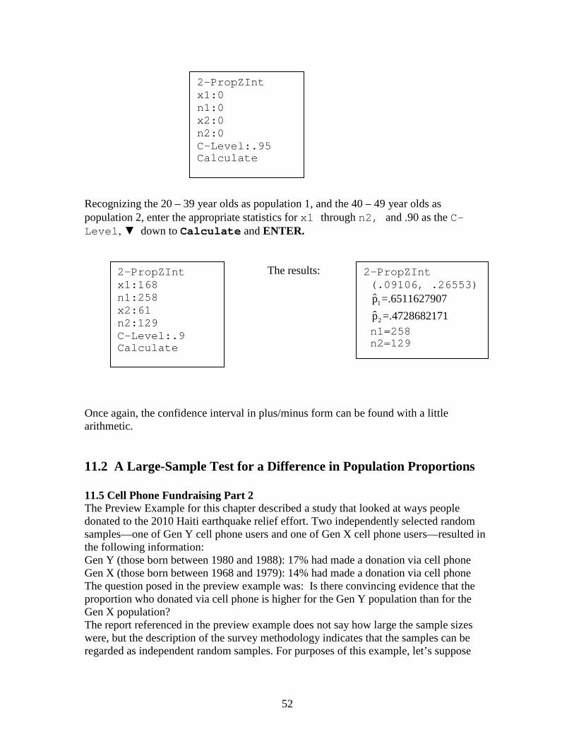
52

2-PropZInt (.09106, .26553)

1

2

p =.6511627907p =.4728682171

n1=258 n2=129

2-PropZInt x1:168 n1:258 x2:61 n2:129 C-Level:.9 Calculate

Recognizing the 20 – 39 year olds as population 1, and the 40 – 49 year olds as population 2, enter the appropriate statistics for x1 through n2, and .90 as the C-Level, ▼ down to Calculate and ENTER.

The results:

Once again, the confidence interval in plus/minus form can be found with a little arithmetic. 11.2 A Large-Sample Test for a Difference in Population Proportions 11.5 Cell Phone Fundraising Part 2 The Preview Example for this chapter described a study that looked at ways people donated to the 2010 Haiti earthquake relief effort. Two independently selected random samples—one of Gen Y cell phone users and one of Gen X cell phone users—resulted in the following information: Gen Y (those born between 1980 and 1988): 17% had made a donation via cell phone Gen X (those born between 1968 and 1979): 14% had made a donation via cell phone The question posed in the preview example was: Is there convincing evidence that the proportion who donated via cell phone is higher for the Gen Y population than for the Gen X population? The report referenced in the preview example does not say how large the sample sizes were, but the description of the survey methodology indicates that the samples can be regarded as independent random samples. For purposes of this example, let’s suppose

2-PropZInt x1:0 n1:0 x2:0 n2:0 C-Level:.95 Calculate

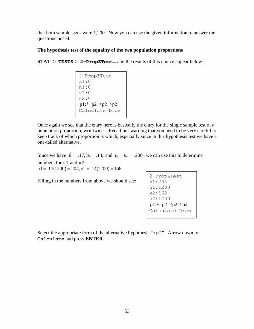
53

that both sample sizes were 1,200. Now you can use the given information to answer the questions posed. The hypothesis test of the equality of the two population proportions STAT > TESTS > 2-PropZTest… and the results of this choice appear below: Once again we see that the entry here is basically the entry for the single sample test of a population proportion, writ twice. Recall our warning that you need to be very careful to keep track of which proportion is which, especially since in this hypothesis test we have a one-tailed alternative. Since we have

1 21 2.17, .14, and 1200p p n n= = = = , we can use this to determine numbers for x1 and x2.

1 .17(1200) 204, 2 .14(1200) 168x x= = = = Filling in the numbers from above we should see: Select the appropriate form of the alternative hypothesis “>p2”. Arrow down to Calculate and press ENTER.

2-PropZTest x1:0 n1:0 x2:0 n2:0 p1: p2 <p2 >p2¹ Calculate Draw

2-PropZTest x1:204 n1:1200 x2:168 n2:1200 p1: p2 <p2 >p2¹ Calculate Draw

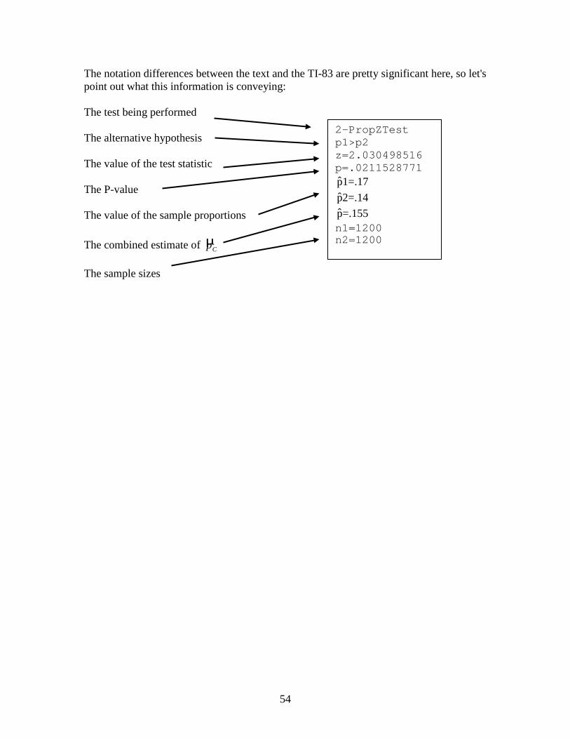
54

2-PropZTest p1>p2 z=2.030498516 p=.0211528771 p1=.17 p2=.14 p=.155 n1=1200 n2=1200

The notation differences between the text and the TI-83 are pretty significant here, so let's point out what this information is conveying: The test being performed The alternative hypothesis The value of the test statistic The P-value The value of the sample proportions The combined estimate of µCp The sample sizes

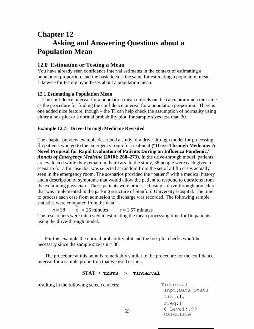
55

Tinterval Inpt:Data Stats List: 1L Freq:1 C-Level:.99 Calculate

Chapter 12 Asking and Answering Questions about a Population Mean 12.0 Estimation or Testing a Mean You have already seen confidence interval estimates in the context of estimating a population proportion, and the basic idea is the same for estimating a population mean. Likewise for testing hypotheses about a population mean. 12.1 Estimating a Population Mean The confidence interval for a population mean unfolds on the calculator much the same as the procedure for finding the confidence interval for a population proportion. There is one added nice feature, though – the TI can help check the assumption of normality using either a box plot or a normal probability plot, for sample sizes less than 30. Example 12.7: Drive-Through Medicine Revisited The chapter preview example described a study of a drive-through model for processing flu patients who go to the emergency room for treatment (“Drive-Through Medicine: A Novel Proposal for Rapid Evaluation of Patients During an Influenza Pandemic,” Annals of Emergency Medicine [2010]: 268–273). In the drive-through model, patients are evaluated while they remain in their cars. In the study, 38 people were each given a scenario for a flu case that was selected at random from the set of all flu cases actually seen in the emergency room. The scenarios provided the “patient” with a medical history and a description of symptoms that would allow the patient to respond to questions from the examining physician. These patients were processed using a drive-through procedure that was implemented in the parking structure of Stanford University Hospital. The time to process each case from admission to discharge was recorded. The following sample statistics were computed from the data:

n = 38 x = 26 minutes s = 1.57 minutes The researchers were interested in estimating the mean processing time for flu patients using the drive-through model. For this example the normal probability plot and the box plot checks won’t be necessary since the sample size is n = 38. The procedure at this point is remarkably similar to the procedure for the confidence interval for a sample proportion that we used earlier: STAT > TESTS > TInterval resulting in the following screen choices:

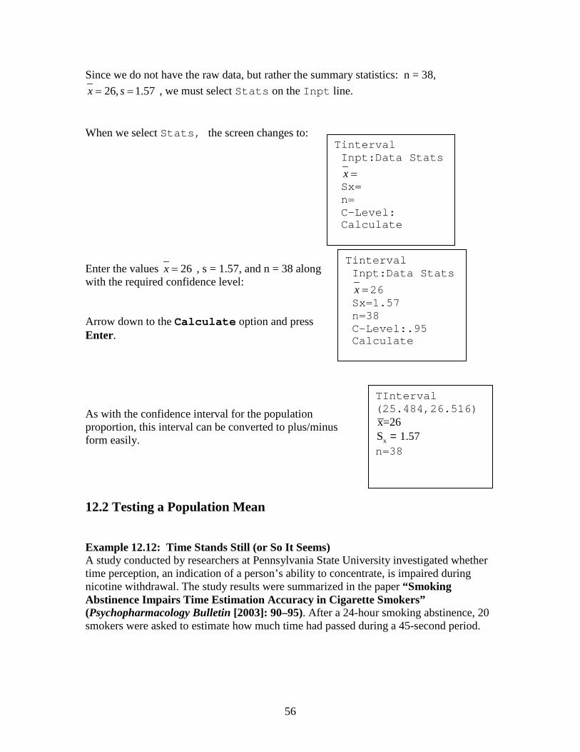
56

TInterval (25.484,26.516) x=26

xS 1.57= n=38

Tinterval Inpt:Data Stats

x = Sx= n= C-Level: Calculate

Tinterval Inpt:Data Stats

x =26 Sx=1.57 n=38 C-Level:.95 Calculate

Since we do not have the raw data, but rather the summary statistics: n = 38, 26, 1.57x s= = , we must select Stats on the Inpt line.

When we select Stats, the screen changes to: Enter the values 26x = , s = 1.57, and n = 38 along with the required confidence level: Arrow down to the Calculate option and press Enter. As with the confidence interval for the population proportion, this interval can be converted to plus/minus form easily. 12.2 Testing a Population Mean Example 12.12: Time Stands Still (or So It Seems) A study conducted by researchers at Pennsylvania State University investigated whether time perception, an indication of a person’s ability to concentrate, is impaired during nicotine withdrawal. The study results were summarized in the paper “Smoking Abstinence Impairs Time Estimation Accuracy in Cigarette Smokers” (Psychopharmacology Bulletin [2003]: 90–95). After a 24-hour smoking abstinence, 20 smokers were asked to estimate how much time had passed during a 45-second period.

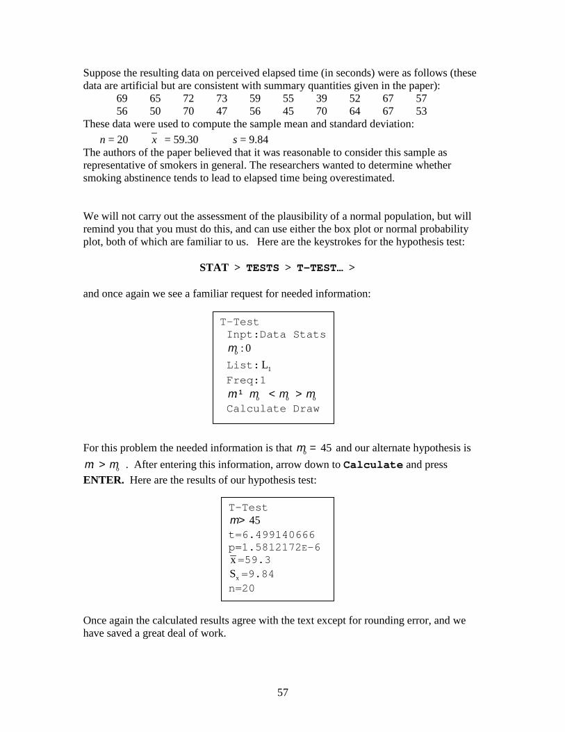
57

Suppose the resulting data on perceived elapsed time (in seconds) were as follows (these data are artificial but are consistent with summary quantities given in the paper):

69 65 72 73 59 55 39 52 67 57 56 50 70 47 56 45 70 64 67 53

These data were used to compute the sample mean and standard deviation: n = 20 x = 59.30 s = 9.84

The authors of the paper believed that it was reasonable to consider this sample as representative of smokers in general. The researchers wanted to determine whether smoking abstinence tends to lead to elapsed time being overestimated. We will not carry out the assessment of the plausibility of a normal population, but will remind you that you must do this, and can use either the box plot or normal probability plot, both of which are familiar to us. Here are the keystrokes for the hypothesis test: STAT > TESTS > T-TEST… > and once again we see a familiar request for needed information: For this problem the needed information is that o 45m = and our alternate hypothesis is

o: m m> . After entering this information, arrow down to Calculate and press ENTER. Here are the results of our hypothesis test: Once again the calculated results agree with the text except for rounding error, and we have saved a great deal of work.

T-Test Inpt:Data Stats : 0om

List: 1L Freq:1 o o o: m m m m¹ < > Calculate Draw

T-Test 45 m>

t=6.499140666 p=1.5812172E-6 x=59.3

xS =9.84 n=20

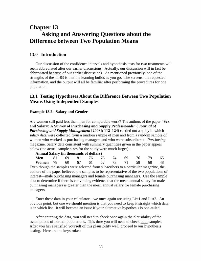
58

Chapter 13 Asking and Answering Questions about the Difference between Two Population Means 13.0 Introduction Our discussion of the confidence intervals and hypothesis tests for two treatments will seem abbreviated after our earlier discussions. Actually, our discussion will in fact be abbreviated because of our earlier discussions. As mentioned previously, one of the strengths of the TI-83 is that the learning builds as you go. The screens, the requested information, and the output will all be familiar after performing the procedures for one population. 13.1 Testing Hypotheses About the Difference Between Two Population Means Using Independent Samples Example 13.2: Salary and Gender Are women still paid less than men for comparable work? The authors of the paper “Sex and Salary: A Survey of Purchasing and Supply Professionals” ( Journal of Purchasing and Supply Management [2008]: 112–124) carried out a study in which salary data were collected from a random sample of men and from a random sample of women who worked as purchasing managers and who were subscribers to Purchasing magazine. Salary data consistent with summary quantities given in the paper appear below (the actual sample sizes for the study were much larger):

Annual Salary (in thousands of dollars) Men 81 69 81 76 76 74 69 76 79 65 Women 78 60 67 61 62 73 71 58 68 48

Even though the samples were selected from subscribers to a particular magazine, the authors of the paper believed the samples to be representative of the two populations of interest—male purchasing managers and female purchasing managers. Use the sample data to determine if there is convincing evidence that the mean annual salary for male purchasing managers is greater than the mean annual salary for female purchasing managers. Enter these data in your calculator – we once again are using List1 and List2. An obvious point, but one we should mention is that you need to keep it straight which data is in which list. It will become an issue if your alternative hypothesis is one-tailed. After entering the data, you will need to check once again the plausibility of the assumptions of normal populations. This time you will need to check both samples. After you have satisfied yourself of this plausibility we'll proceed to our hypothesis testing. Here are the keystrokes:

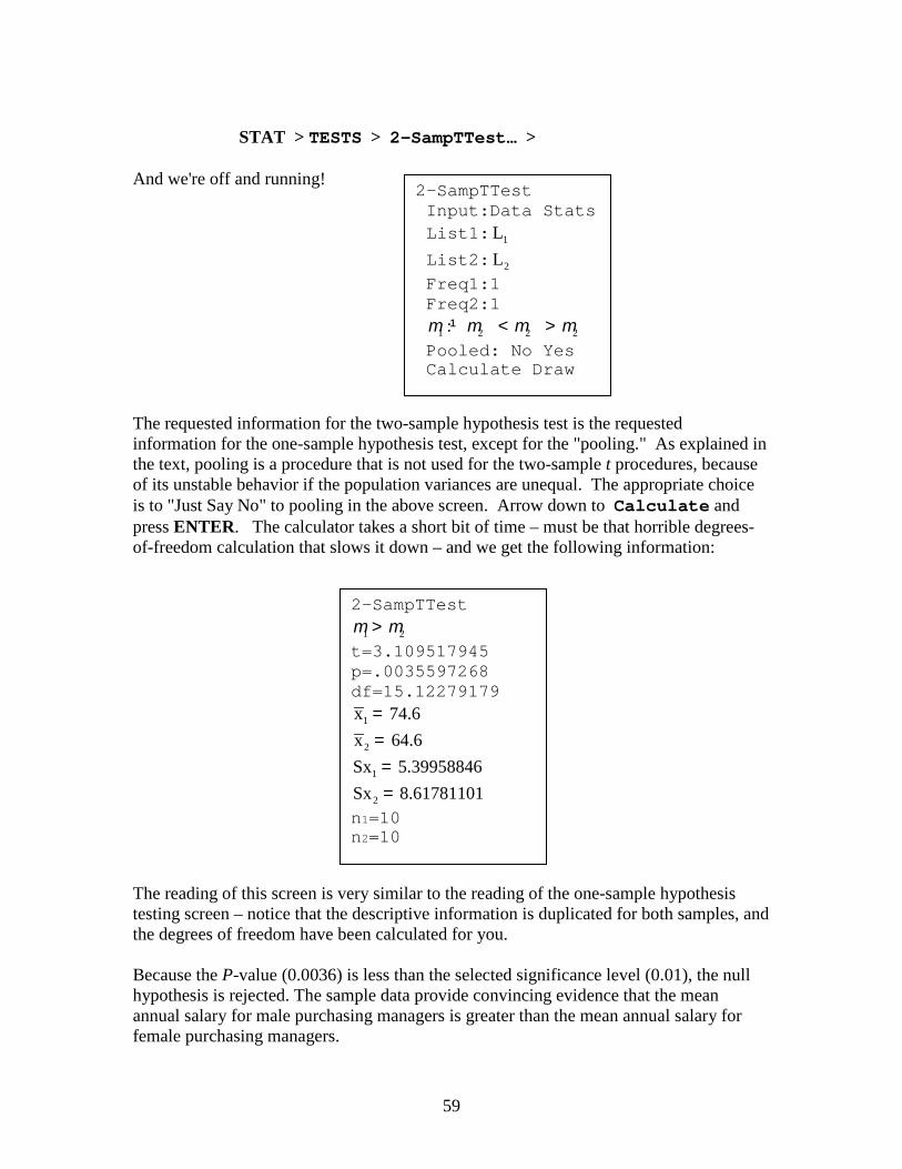
59

STAT > TESTS > 2-SampTTest… > And we're off and running! The requested information for the two-sample hypothesis test is the requested information for the one-sample hypothesis test, except for the "pooling." As explained in the text, pooling is a procedure that is not used for the two-sample t procedures, because of its unstable behavior if the population variances are unequal. The appropriate choice is to "Just Say No" to pooling in the above screen. Arrow down to Calculate and press ENTER. The calculator takes a short bit of time – must be that horrible degrees-of-freedom calculation that slows it down – and we get the following information: The reading of this screen is very similar to the reading of the one-sample hypothesis testing screen – notice that the descriptive information is duplicated for both samples, and the degrees of freedom have been calculated for you. Because the P-value (0.0036) is less than the selected significance level (0.01), the null hypothesis is rejected. The sample data provide convincing evidence that the mean annual salary for male purchasing managers is greater than the mean annual salary for female purchasing managers.

2-SampTTest Input:Data Stats List1: 1L

List2: 2L Freq1:1 Freq2:1 1 2 2 2: m m m m¹ < > Pooled: No Yes Calculate Draw

2-SampTTest

1 2m m> t=3.109517945 p=.0035597268 df=15.12279179

1x 74.6=

2x 64.6=

1Sx 5.39958846=

2Sx 8.61781101= n1=10 n2=10

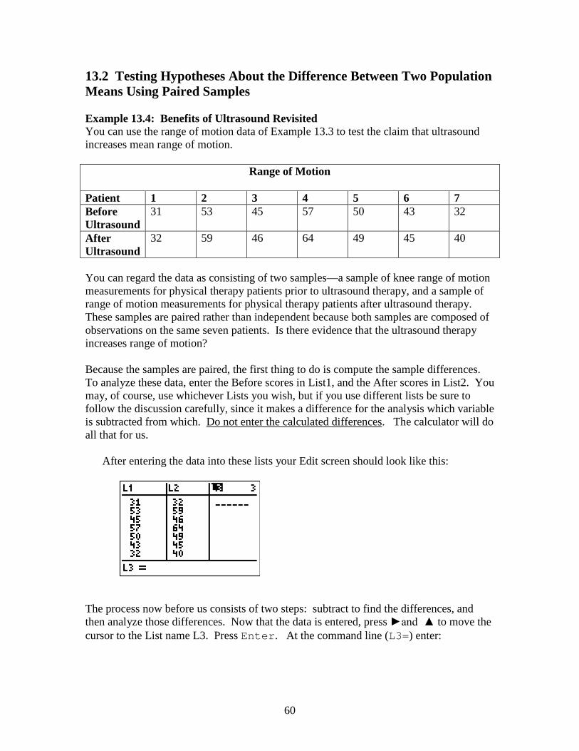
60

13.2 Testing Hypotheses About the Difference Between Two Population Means Using Paired Samples Example 13.4: Benefits of Ultrasound Revisited You can use the range of motion data of Example 13.3 to test the claim that ultrasound increases mean range of motion.

Range of Motion Patient 1 2 3 4 5 6 7 Before Ultrasound

31 53 45 57 50 43 32

After Ultrasound

32 59 46 64 49 45 40

You can regard the data as consisting of two samples—a sample of knee range of motion measurements for physical therapy patients prior to ultrasound therapy, and a sample of range of motion measurements for physical therapy patients after ultrasound therapy. These samples are paired rather than independent because both samples are composed of observations on the same seven patients. Is there evidence that the ultrasound therapy increases range of motion? Because the samples are paired, the first thing to do is compute the sample differences. To analyze these data, enter the Before scores in List1, and the After scores in List2. You may, of course, use whichever Lists you wish, but if you use different lists be sure to follow the discussion carefully, since it makes a difference for the analysis which variable is subtracted from which. Do not enter the calculated differences. The calculator will do all that for us. After entering the data into these lists your Edit screen should look like this:

The process now before us consists of two steps: subtract to find the differences, and then analyze those differences. Now that the data is entered, press ►and ▲ to move the cursor to the List name L3. Press Enter. At the command line (L3=) enter:

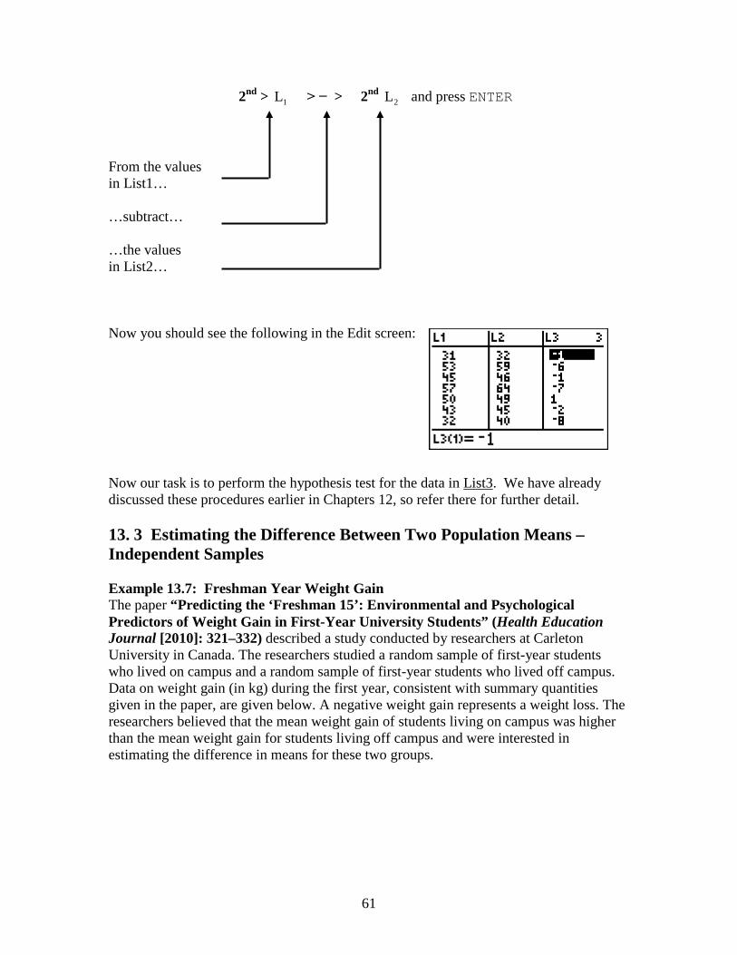
61

2nd > 1L > − > 2nd 2L and press ENTER From the values in List1… …subtract… …the values in List2… Now you should see the following in the Edit screen: Now our task is to perform the hypothesis test for the data in List3. We have already discussed these procedures earlier in Chapters 12, so refer there for further detail. 13. 3 Estimating the Difference Between Two Population Means – Independent Samples Example 13.7: Freshman Year Weight Gain The paper “Predicting the ‘Freshman 15’: Environmental and Psychological Predictors of Weight Gain in First-Year University Students” (Health Education Journal [2010]: 321–332) described a study conducted by researchers at Carleton University in Canada. The researchers studied a random sample of first-year students who lived on campus and a random sample of first-year students who lived off campus. Data on weight gain (in kg) during the first year, consistent with summary quantities given in the paper, are given below. A negative weight gain represents a weight loss. The researchers believed that the mean weight gain of students living on campus was higher than the mean weight gain for students living off campus and were interested in estimating the difference in means for these two groups.

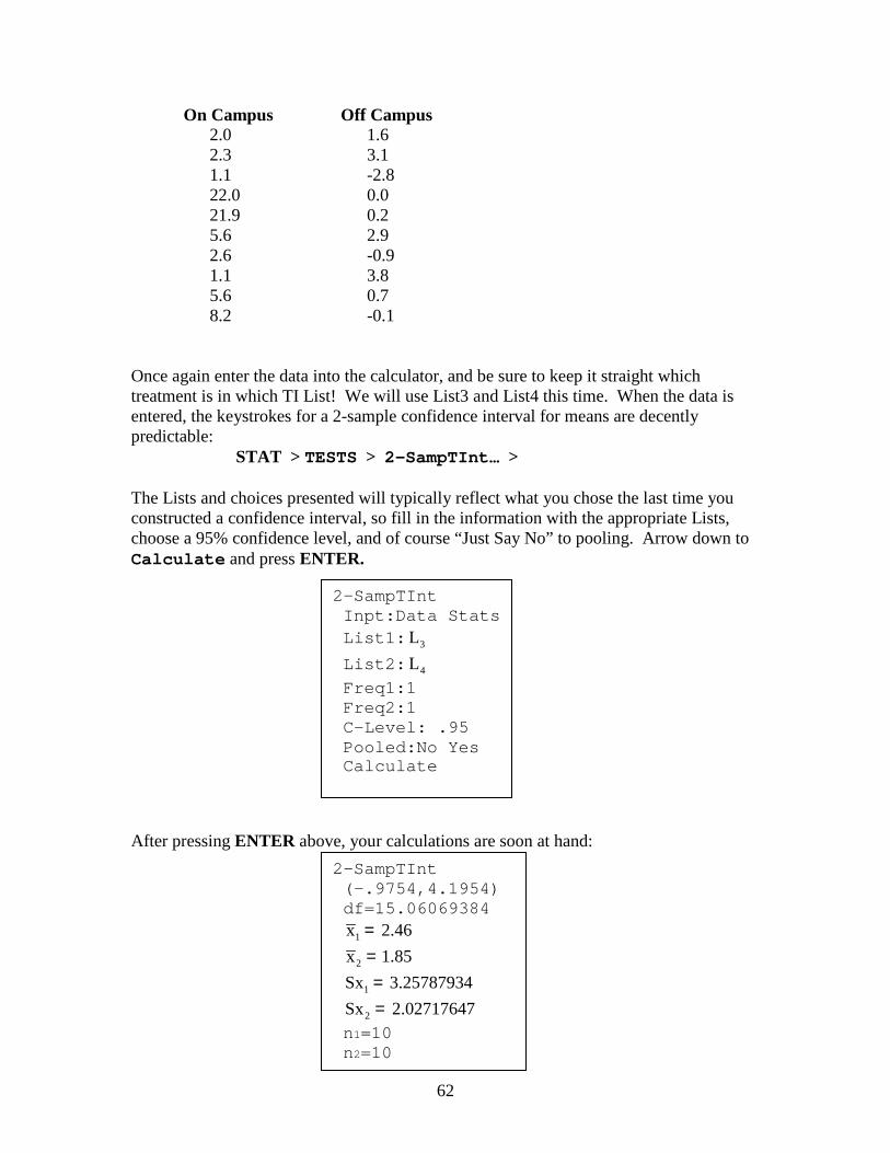
62

On Campus Off Campus 2.0 1.6 2.3 3.1 1.1 -2.8 22.0 0.0 21.9 0.2 5.6 2.9 2.6 -0.9 1.1 3.8 5.6 0.7 8.2 -0.1

Once again enter the data into the calculator, and be sure to keep it straight which treatment is in which TI List! We will use List3 and List4 this time. When the data is entered, the keystrokes for a 2-sample confidence interval for means are decently predictable:

STAT > TESTS > 2-SampTInt… > The Lists and choices presented will typically reflect what you chose the last time you constructed a confidence interval, so fill in the information with the appropriate Lists, choose a 95% confidence level, and of course “Just Say No” to pooling. Arrow down to Calculate and press ENTER. After pressing ENTER above, your calculations are soon at hand:

2-SampTInt Inpt:Data Stats List1: 3L

List2: 4L Freq1:1 Freq2:1 C-Level: .95 Pooled:No Yes Calculate

2-SampTInt (-.9754,4.1954) df=15.06069384 1x 2.46=

2x 1.85=

1Sx 3.25787934=

2Sx 2.02717647= n1=10 n2=10

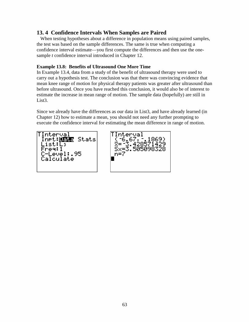
63

13. 4 Confidence Intervals When Samples are Paired When testing hypotheses about a difference in population means using paired samples, the test was based on the sample differences. The same is true when computing a confidence interval estimate—you first compute the differences and then use the one-sample t confidence interval introduced in Chapter 12. Example 13.8: Benefits of Ultrasound One More Time In Example 13.4, data from a study of the benefit of ultrasound therapy were used to carry out a hypothesis test. The conclusion was that there was convincing evidence that mean knee range of motion for physical therapy patients was greater after ultrasound than before ultrasound. Once you have reached this conclusion, it would also be of interest to estimate the increase in mean range of motion. The sample data (hopefully) are still in List3. Since we already have the differences as our data in List3, and have already learned (in Chapter 12) how to estimate a mean, you should not need any further prompting to execute the confidence interval for estimating the mean difference in range of motion.

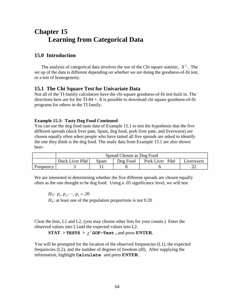
64

Chapter 15 Learning from Categorical Data 15.0 Introduction The analysis of categorical data involves the use of the Chi square statistic, 2X . The set up of the data is different depending on whether we are doing the goodness-of-fit test, or a test of homogeneity. 15.1 The Chi Square Test for Univariate Data Not all of the TI-family calculators have the chi-square goodness-of-fit test built in. The directions here are for the TI-84 +. It is possible to download chi square goodness-of-fit programs for others in the TI family. Example 15.3: Tasty Dog Food Continued You can use the dog food taste data of Example 15.1 to test the hypothesis that the five different spreads (duck liver pate, Spam, dog food, pork liver pate, and liverwurst) are chosen equally often when people who have tasted all five spreads are asked to identify the one they think is the dog food. The study data from Example 15.1 are also shown here:

We are interested in determining whether the five different spreads are chosen equally often as the one thought to be dog food. Using a .05 significance level, we will test

H0: 1 2 5, , , .20p p p = Ha: at least one of the population proportions is not 0.20

Clear the lists, L1 and L2, (you may choose other lists for your counts.) Enter the observed values into L1and the expected values into L2.

STAT > TESTS > 2χ GOF-Test , and press ENTER. You will be prompted for the location of the observed frequencies (L1), the expected frequencies (L2), and the number of degrees of freedom (df). After supplying the information, highlight Calculate and press ENTER.

Spread Chosen as Dog Food Duck Liver Pâté Spam Dog Food Pork Liver Pâté Liverwurst Frequency 3 11 8 6 22

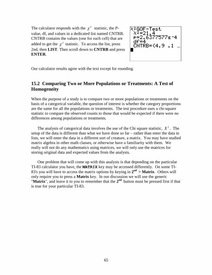
65

The calculator responds with the 2χ statistic, the P-value, df, and values in a dedicated list named CNTRB. CNTRB contains the values (one for each cell) that are added to get the 2χ statistic. To access the list, press 2nd, then LIST. Then scroll down to CNTRB and press ENTER. Our calculator results agree with the text except for rounding. 15.2 Comparing Two or More Populations or Treatments: A Test of Homogeneity When the purpose of a study is to compare two or more populations or treatments on the basis of a categorical variable, the question of interest is whether the category proportions are the same for all the populations or treatments. The test procedure uses a chi-square statistic to compare the observed counts to those that would be expected if there were no differences among populations or treatments. The analysis of categorical data involves the use of the Chi square statistic, 2X . The setup of the data is different than what we have done so far – rather than enter the data in lists, we will enter the data in a different sort of creature, a matrix. You may have studied matrix algebra in other math classes, or otherwise have a familiarity with them. We really will not do any mathematics using matrices, we will only use the matrices for storing original data and expected values from the analysis. One problem that will come up with this analysis is that depending on the particular TI-83 calculator you have, the MATRIX key may be accessed differently. On some TI-83's you will have to access the matrix options by keying in 2nd > Matrix. Others will only require you to press a Matrix key. In our discussion we will use the generic "Matrix", and leave it to you to remember that the 2nd button must be pressed first if that is true for your particular TI-83.

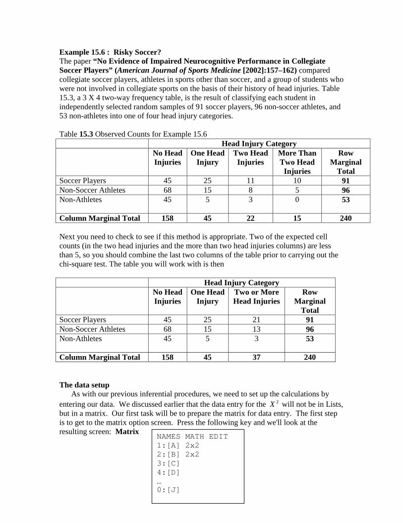
66

Example 15.6 : Risky Soccer? The paper “No Evidence of Impaired Neurocognitive Performance in Collegiate Soccer Players” (American Journal of Sports Medicine [2002]:157–162) compared collegiate soccer players, athletes in sports other than soccer, and a group of students who were not involved in collegiate sports on the basis of their history of head injuries. Table 15.3, a 3 X 4 two-way frequency table, is the result of classifying each student in independently selected random samples of 91 soccer players, 96 non-soccer athletes, and 53 non-athletes into one of four head injury categories. Table 15.3 Observed Counts for Example 15.6 Head Injury Category No Head

Injuries One Head

Injury Two Head

Injuries More Than Two Head

Injuries

Row Marginal

Total Soccer Players 45 25 11 10 91 Non-Soccer Athletes 68 15 8 5 96 Non-Athletes 45 5 3 0 53

Column Marginal Total 158 45 22 15 240 Next you need to check to see if this method is appropriate. Two of the expected cell counts (in the two head injuries and the more than two head injuries columns) are less than 5, so you should combine the last two columns of the table prior to carrying out the chi-square test. The table you will work with is then Head Injury Category No Head

Injuries One Head

Injury Two or More Head Injuries

Row Marginal

Total Soccer Players 45 25 21 91 Non-Soccer Athletes 68 15 13 96 Non-Athletes 45 5 3 53

Column Marginal Total 158 45 37 240 The data setup As with our previous inferential procedures, we need to set up the calculations by entering our data. We discussed earlier that the data entry for the 2X will not be in Lists, but in a matrix. Our first task will be to prepare the matrix for data entry. The first step is to get to the matrix option screen. Press the following key and we'll look at the resulting screen: Matrix

NAMES MATH EDIT 1:[A] 2x2 2:[B] 2x2 3:[C] 4:[D] … 0:[J]

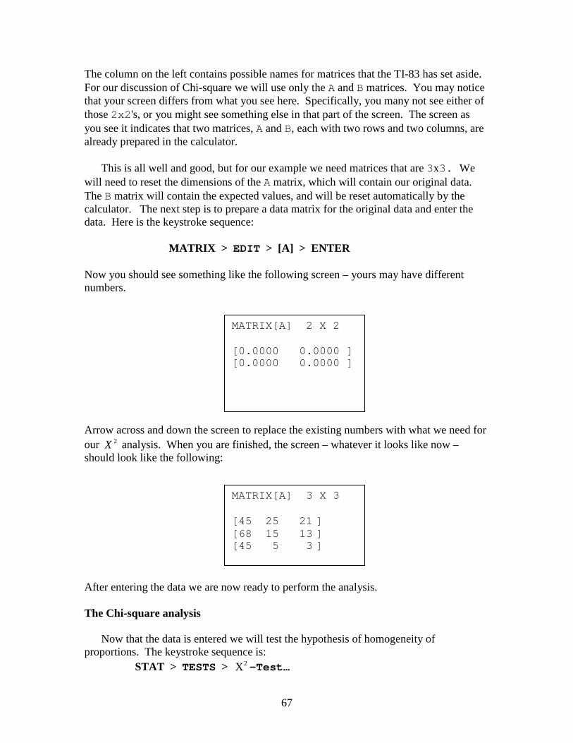
67

The column on the left contains possible names for matrices that the TI-83 has set aside. For our discussion of Chi-square we will use only the A and B matrices. You may notice that your screen differs from what you see here. Specifically, you many not see either of those 2x2's, or you might see something else in that part of the screen. The screen as you see it indicates that two matrices, A and B, each with two rows and two columns, are already prepared in the calculator. This is all well and good, but for our example we need matrices that are 3x3. We will need to reset the dimensions of the A matrix, which will contain our original data. The B matrix will contain the expected values, and will be reset automatically by the calculator. The next step is to prepare a data matrix for the original data and enter the data. Here is the keystroke sequence: MATRIX > EDIT > [A] > ENTER Now you should see something like the following screen – yours may have different numbers. Arrow across and down the screen to replace the existing numbers with what we need for our 2X analysis. When you are finished, the screen – whatever it looks like now – should look like the following: After entering the data we are now ready to perform the analysis. The Chi-square analysis Now that the data is entered we will test the hypothesis of homogeneity of proportions. The keystroke sequence is: STAT > TESTS > 2X -Test…

MATRIX[A] 2 X 2 [0.0000 0.0000 ] [0.0000 0.0000 ]

MATRIX[A] 3 X 3 [45 25 21 ] [68 15 13 ] [45 5 3 ]

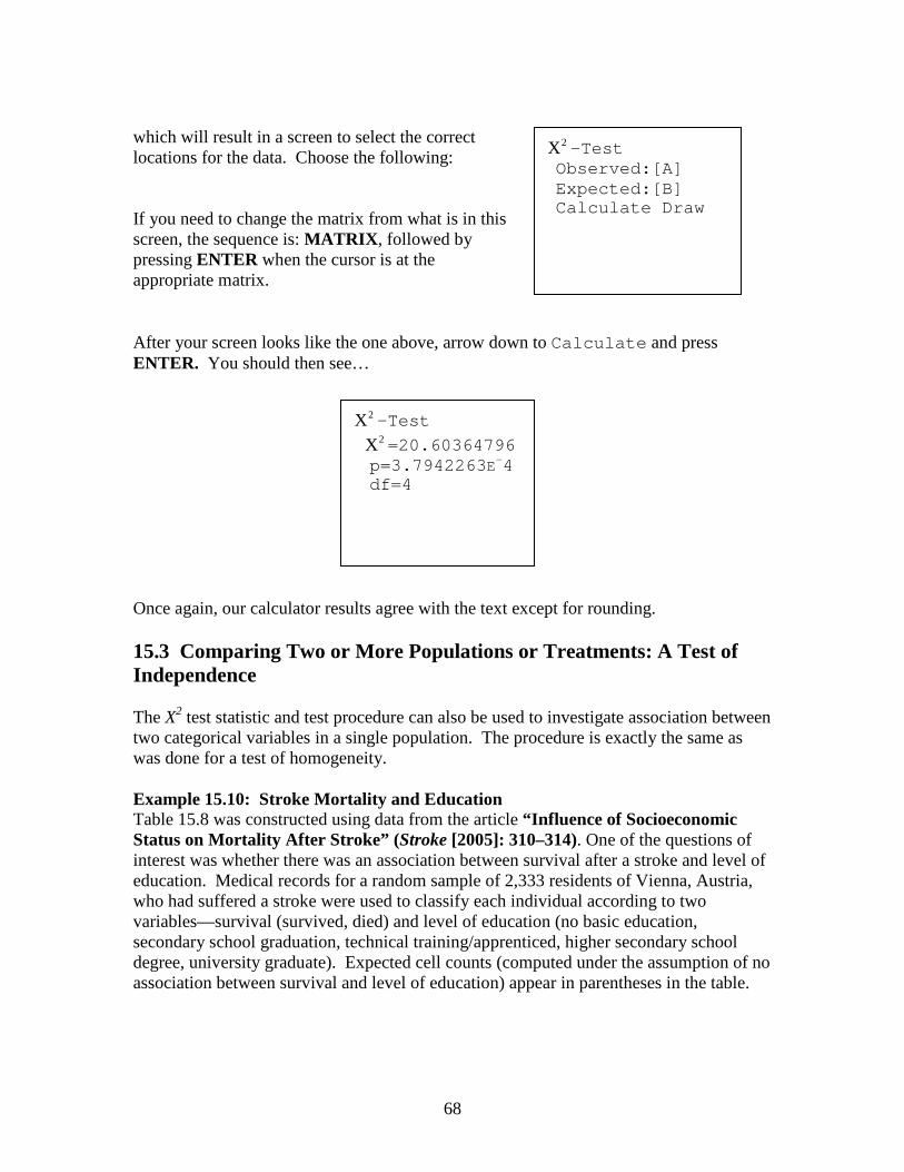
68

2X -Test Observed:[A] Expected:[B] Calculate Draw

which will result in a screen to select the correct locations for the data. Choose the following: If you need to change the matrix from what is in this screen, the sequence is: MATRIX, followed by pressing ENTER when the cursor is at the appropriate matrix. After your screen looks like the one above, arrow down to Calculate and press ENTER. You should then see… Once again, our calculator results agree with the text except for rounding. 15.3 Comparing Two or More Populations or Treatments: A Test of Independence The X2 test statistic and test procedure can also be used to investigate association between two categorical variables in a single population. The procedure is exactly the same as was done for a test of homogeneity. Example 15.10: Stroke Mortality and Education Table 15.8 was constructed using data from the article “Influence of Socioeconomic Status on Mortality After Stroke” (Stroke [2005]: 310–314). One of the questions of interest was whether there was an association between survival after a stroke and level of education. Medical records for a random sample of 2,333 residents of Vienna, Austria, who had suffered a stroke were used to classify each individual according to two variables—survival (survived, died) and level of education (no basic education, secondary school graduation, technical training/apprenticed, higher secondary school degree, university graduate). Expected cell counts (computed under the assumption of no association between survival and level of education) appear in parentheses in the table.

2X -Test 2X =20.60364796 p=3.7942263E-4 df=4

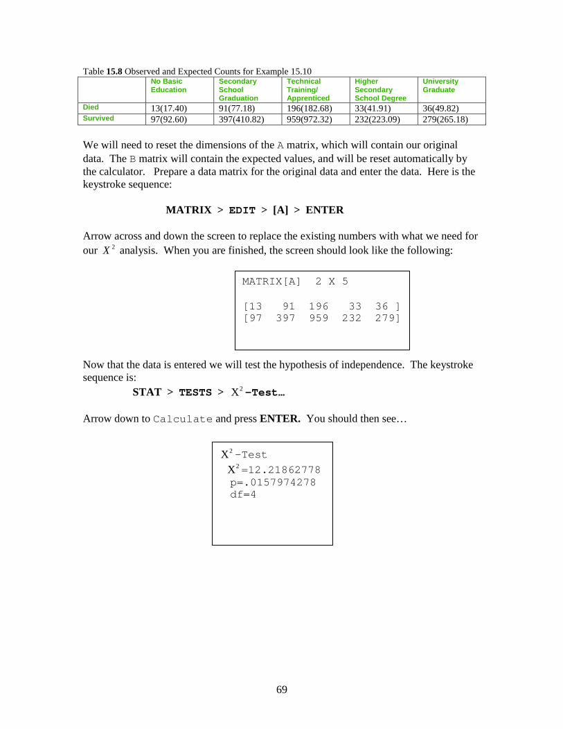
69

MATRIX[A] 2 X 5 [13 91 196 33 36 ] [97 397 959 232 279]

Table 15.8 Observed and Expected Counts for Example 15.10 No Basic

Education Secondary School Graduation

Technical Training/ Apprenticed

Higher Secondary School Degree

University Graduate

Died 13(17.40) 91(77.18) 196(182.68) 33(41.91) 36(49.82) Survived 97(92.60) 397(410.82) 959(972.32) 232(223.09) 279(265.18) We will need to reset the dimensions of the A matrix, which will contain our original data. The B matrix will contain the expected values, and will be reset automatically by the calculator. Prepare a data matrix for the original data and enter the data. Here is the keystroke sequence: MATRIX > EDIT > [A] > ENTER Arrow across and down the screen to replace the existing numbers with what we need for our 2X analysis. When you are finished, the screen should look like the following: Now that the data is entered we will test the hypothesis of independence. The keystroke sequence is: STAT > TESTS > 2X -Test… Arrow down to Calculate and press ENTER. You should then see…

2X -Test 2X =12.21862778 p=.0157974278 df=4