University of ConnecticutOpenCommons@UConn

Doctoral Dissertations University of Connecticut Graduate School

4-20-2017

Three Essays on the Efficiency of Carbon EmissionTrading ProgramsYishu Zhouyishu.zhou@uconn.edu

Follow this and additional works at: https://opencommons.uconn.edu/dissertations

Recommended CitationZhou, Yishu, "Three Essays on the Efficiency of Carbon Emission Trading Programs" (2017). Doctoral Dissertations. 1417.https://opencommons.uconn.edu/dissertations/1417

Three Essays on the Efficiency of Carbon Emission Trading Programs

Yishu Zhou, PhD

University of Connecticut, 2017

Using individual level data from electricity generators, my dissertation empirically inves-

tigates the effectiveness of existing regional environmental policies in the U.S. electricity

wholesale markets aiming to reduce CO2 emissions. Big drop of natural gas price and

limited magnitude and variation of CO2 allowance prices make the contribution of CO2

cap and trade programs questionable. Given the complexity of the electricity markets,

the central of my research is to decompose the co-existing various effects on individual

firms’ emissions and evaluate the performance of current regional regulations. I particu-

larly study the Regional Greenhouse Gas Initiative (RGGI), which regulates power plants

in nine northeastern states of the U.S.. The first chapter measures the impact of carbon

emission regulation on U.S. power plants’ technical efficiency. No evidence of technical

efficiency changes due to the RGGI regime in the RGGI area is found. Using a difference-

in-difference framework in chapter two, we find that overall the RGGI program leads to

7.72 million short tons of CO2 reduction per year in Delaware and Maryland, or about

34.36% of the average total annual emissions in these two states. All utilities respond to

the program by decreasing their heat input per capacity even including natural gas utili-

ties. Chapter 3 studies electricity generators’ production behavior and how the decisions

are altered with CO2 emission regulations. The results show that the RGGI policy has

helped to decrease the total CO2 emissions by at least 4.73% during the sample period.

All other things equal, an additional $1/ton increase in permit price reduce the total CO2

emissions by 1.85%.

Three Essays on the Efficiency of Carbon Emission Trading Programs

Yishu Zhou

B.A., Nanjing University, 2009

M.A., University of Illinois at Urbana-Champaign, 2010

A Dissertation

Submitted in Partial Fulfillment of the

Requirements for the Degree of

Doctor of Philosophy

at the

University of Connecticut

2017

i

Copyright by

Yishu Zhou

2017

ii

APPROVAL PAGE

Doctor of Philosophy Dissertation

Three Essays on the Efficiency of Carbon Emission Trading Programs

Presented by

Yishu Zhou, B.A., M.A.

Major Advisor __________________________________________________________

Ling Huang

Associate Advisor ______________________________________________________

Kathleen Segerson

Associate Advisor ______________________________________________________

Talia Bar

University of Connecticut

2017

iii

TABLE OF CONTENTS

Overview . . . . . . . . . . . . . . . . . . . . . . . . . . . . . . . . . . . . . . . . . . . . . . . . . . . . . . . . . . . . . . . . . . . . . . . . . . . . .1

Chapter One: Have U.S. Power Plants Become Less Technically Efficient? The Impact of

Carbon Emission Regulation. . . . . . . . . . . . . . . . . . . . . . . . . . . . . . . . . . . . . . . . . . . . . . . . . . . . . . . . . . 7

Chapter Two: Carbon Prices and Fuel Switching: A Quasi-experiment in Electricity

Markets . . . . . . . . . . . . . . . . . . . . . . . . . . . . . . . . . . . . . . . . . . . . . . . . . . . . . . . . . . . . . . . . . . . . . . . . . . . . .31

Chapter Three: Emission Responses to Carbon Pricing in Dynamic Electricity Markets . .

. . . . . . . . . . . . . . . . . . . . . . . . . . . . . . . . . . . . . . . . . . . . . . . . . . . . . . . . . . . . . . . . . . . . . . . . . . 69

iv

Overview

Market-based emission trading programs have been widely adopted around the world

since 1990s. The first national emissions cap and trade program in the U.S. is the Acid

Rain Program (ARP), established under Title IV of the 1990 Clean Air Act (CAA) Amend-

ments. It requires power plants to reduce emissions of sulfur dioxide (SO2) and nitro-

gen oxides (NOx), the primary precursors of acid rain. However, similar programs for

greenhouse gas (GHG) emissions were not established until rather recently. European

Union Emissions Trading Scheme (EU ETS) is the first and largest GHG emissions trading

scheme in the world. In the U.S., although lacking of regulations at national level, some

regional programs have been formed, such as the Regional Greenhouse Gas Initiative

(RGGI) and the Western Climate Initiative (WCI). On June 2, 2014, United States Envi-

ronmental Protection Agency (EPA) proposed a nationwide plan to cut carbon pollution

from power plants in all states. The study of existing regional GHG emission trading pro-

grams can provide important guidelines for future regulations, at both regional and federal

levels.

The focus of my dissertation is on RGGI. RGGI is a cooperative effort to reduce CO2

emissions among the states of Connecticut, Delaware, Maine, Maryland, Massachusetts,

New Hampshire, New York, Rhode Island, and Vermont specifically in the electric power

sector.1 Regulated sources are fossil fuel-fired power plants with a capacity of 25 MW

or greater located within the RGGI States. RGGI aims to stabilize and then reduce CO2

emissions within the signatory states. The effort was formally initiated in 2003 and the

compliance started on January 1st, 2009. Every control period lasts three years, at the

end of the third year of a control period, each regulated plant is required to hold one

allowance for each ton of CO2 emitted. During a control period, unused allowances will not

expire and can be banked for future years. If a plant violates the rule, it needs to surrender

a number of allowances equal to three times the number of its excess emissions. More1New Jersey withdrew from the program at the end of year 2011.

1

than 90% of the allowances are sold at RGGI quarterly auctions. Through the end of

2013, RGGI has conducted 22 successful auctions, selling a total of 651 million CO2

allowances for $1.6 billion. Proceeds from the auctions are returned to states and invested

in consumer benefit programs such as energy efficiency and renewable resources. The

annual emission cap, which is the total allowances allocated each year, is decreasing over

time.

According to RGGI (2014), average CO2 emissions from 2010-2012 in RGGI states

decreased by 25.4%, compared with the average from 2006-2008. In addition, the CO2

emission rate (pounds of CO2 per megawatt hour) dropped by 16.7% during the same

period. There are four major methods to reduce CO2 emissions: The first is to reduce

demand of electricity generated by fossil fuel plants, such as energy efficiency programs

and increase use of renewable resources in electricity generation. The second is to use

more natural gas and less coal (fuel switching), given that burning coal generates twice

as much CO2 as burning natural gas when producing the same amount of heat. The third

method is to increase the efficiency in electricity generation, i.e., generate more electricity

with the same set of inputs. Last but not least, The development of carbon capture and

sequestration allows firms to store CO2 underground, which prevents the release of CO2

into the atmosphere.

In this dissertation I explore several issues related with RGGI. First, the effectiveness

of RGGI has been criticized due to its low CO2 allowance price. The CO2 price was

around only $2 per short ton from 2009 to 2013, it was at or very close to the price floor

set by the program. The low permit price was the result of excess supply of CO2 permits

for the first several years of the program. From 2006 to 2008, the average annual CO2

emissions are 163 million short tons. However, the emissions cap set by RGGI was 188

million short tons per year from 2009-2011 and 165 million short tons per year from 2012-

2013. To make the carbon policy more effective, the regulator adjusted cap by decreasing

the number of permits issued each year. For example, the adjusted cap was only 83

2

million short tons in 2014 and 62 million short tons in 2017. Therefore, it is important to

understand how fossil fuel generation and CO2 emissions respond to various allowance

price levels, especially when the price is high.

Second, although CO2 emissions decreased significantly after 2009 in regulated states,

it is still unclear whether the emission reduction is due to the RGGI program. Starting

from 2009, the price of natural gas has plummeted with the development of shale gas

extraction. Decrease of demand or increase of renewable capacity could also lead to

CO2 emission reduction. These effects all drive emissions down. As an evidence, CO2

emissions in both regulated and unregulated states have declined after 2009. In addition,

a general concern of all regional emission trading programs is emission leakage, which

is the increase in emissions in neighboring unregulated states. Last but not least, envi-

ronmental regulations provide power plants with extra incentives to increase production

efficiency, i.e., producing more electricity with less heat. However, RGGI could undermine

power plants’ production efficiency as it is an additional constraint imposed on production

process. If this is true, the decrease in production efficiency cannot be ignored and it

attenuates the effectiveness of the RGGI program. Studies on these topics shed light on

the real impact of RGGI on CO2 emissions and provide important guidelines and caveat

for future regulations at both the state and federal level.

Summary

This dissertation is organized as follows: Chapter 1 estimates power plants’ production

efficiency and evaluates the impact of RGGI policy on the efficiency of coal and natural

gas plants located within both RGGI regulated area and neighboring states. By using

the directional distance function, we find that overall the power sector is highly efficient:

The average technical efficiency scores for coal and natural gas plants are 88.70% and

83.14% respectively. The results show that overtime all power plants become more effi-

cient. There is no clear evidence of RGGI undermining technical efficiency for both fuel

3

types of plants in the RGGI area. However, the policy decreases the technical efficiency

for coal plants within neighboring states. A likely explanation is that since the neigh-

boring states are not regulated by the RGGI policy, plants with lower production cost in

neighboring states, such as coal plants, could produce more than usual due to a spillover

effect. Increased production activities may result in more malfunctions and less frequency

of maintenance, leading to a decreased level of technical efficiency. In RGGI regulated

area, less efficient coal plants exited and more efficient natural gas plants entered after

2009.

Chapter 2 uses difference in difference (DID) estimation to analyze RGGI’s impact on

the electric sector’s fuel switching behavior at both plant and firm levels. We find that

overall the RGGI program leads to 7.72 million short tons of CO2 reduction per year in

Delaware and Maryland, or about 34.36% of the average total annual emissions in these

two states from 2009 to 2013. We find little evidence that utilities adjust their capacities

within five years after program implementation except natural gas-only utilities. All utili-

ties respond to the program by decreasing the utilization rate even including natural gas

utilities. However, the emission reduction achieved through less coal and natural gas gen-

eration in RGGI area is covered by emission leakage instead of fuel switching from dirtier

to cleaner energy sources. The results suggest that the power utilities do respond to the

emission trading program with current carbon prices, but tremendous fuel switching did

not occur before 2013 due to the program as it is less costly to leak the emissions under

the regional regime.

In Chapter 3, I take advantage of the detailed hourly data to investigate how much

of the emission reduction can be attributed to the RGGI policy and how individual firms

respond to more stringent carbon policies. By accounting for the intertemporal production

constraints across hours, I find that the RGGI policy has helped to decrease the total CO2

emissions by at least 4.73% from 2009 to 2013. the relationship between each genera-

tor’s production and the price-cost markup at hourly level and how the producers respond

4

as CO2 price changes. CO2 can be reduced by 23.50% if carbon is priced at $15/ton.

Future Work

The average annual total CO2 emissions of Delaware and Maryland are 42.4 and

29 million short tons from 2006-2008 and 2009-2013 respectively, i.e., after 2009 the

annual emissions have decreased by 46.21% of the average level from 2009-2013. Using

different methods, Chapter 2 and Chapter 3 both examine the effectiveness of the RGGI

policy: How much of the observed emission reduction is attributed to RGGI rather than

the price drop of natural gas? The data used in Chapter 2 are year-round from 2002 to

2013, while chapter 3 only include the data from every September and October of each

year due to the computation burden with detailed hourly data. In both chapters, the data

include the major states in the PJM market, in which only Delaware and Maryland are

regulated by the RGGI program. The treatment group includes power plants in Delaware

and Maryland, while the control group consists of all other plants in the PJM.

Both chapters conclude that the RGGI policy was effective during the sample period

2009-2013. However, there is notable discrepancy in estimates from two models. In

Chapter 2, we find that on average the RGGI program leads to about 34.36% of the

average total annual emissions in Delaware and Maryland from 2009 to 2013, compared

to the conterfactual scenario if there was no RGGI policy. In Chapter 3 I investigate the

same issue with another approach and the emission reduction caused by RGGI in the two

regulated states is only 4.73% from 2009 to 2013. Although the choices of both data and

model differ in the two chapters, this discrepancy is large and deserves more concerns.

Possible explanations for the wide range of estimates need to be further investigated in

the future.

I also plan to adjust the current model in Chapter 3 to accommodate more features in

the electricity markets. Chapter 3 examines how individual firms change production and

emission decisions in response to higher CO2 prices, while keeping other factors constant.

5

An reasonable interpretation is that less profit caused by the extra cost of CO2 permits

provides the electricity industry with more incentives to switch to cleaner fuels. However,

this incentive is weakened if the electricity prices rises along with the CO2 permit prices,

and leaves firms’ profit unchanged. Therefore, the pass-through rate, which measures

how much of the additional emissions cost is passed-through to electricity prices, is an

important part that needs to be added to the existing model (Fabra and Reguant, 2014).

Electricity prices could also be affected by market power. Although Chapter 3 illus-

trates the detailed market power mitigation actions taken by the market regulator and

argues the market is very close to perfect competition, market power is generally an im-

portant concern in many electricity markets. If some big firms are manipulators of the

market clearing prices rather than price takers, then the level of non-fossil fuel generation

would also influence firms fossil-fuel production decisions and market prices. There are

important aspects to explore in the future.

6

Chapter One

Have U.S. Power Plants Become Less Technically Efficient?

The Impact of Carbon Emission Regulation

Yishu Zhou

University of Connecticut

Ling Huang

University of Connecticut

Abstract

We estimate directional distance functions to measure the impact of carbon emission

regulation, the Regional Greenhouse Gas Initiative (RGGI) in particular, on U.S. power

plants’ technical efficiency. The model shows that the average technical efficiency scores

for coal and natural gas plants are 88.70% and 83.14% respectively, indicating a very

technically efficient industry. We find no evidence of technical efficiency changes due

to the RGGI regime in the RGGI area. In the same area, relatively less efficient coal

plants exited the market and slightly more efficient natural gas plants entered, compared

to the incumbent plants. In addition, some evidence of a spillover effect is found. Using

a counterfactual analysis, the RGGI regulation leads to a 1.48% decline in the average

technical efficiency for coal plants within neighboring states of RGGI during 2009-2013.

Keywords: Carbon Emission Regulations; RGGI; Technical Efficiency

7

Introduction

The economic burden of environmental regulations has been debated among economists

and U.S. policy-makers since the beginning of stringent pollution restrictions in the 1970s

(Jaffe et al., 1995). The conventional wisdom is that as partial inputs are diverted to pro-

duce extra environmental goods, environmental regulations can reduce firms’ productivity,

operating efficiency and competitiveness, while other scholars argue a net positive impact

for some industries (Gollop and Roberts, 1983; Jaffe et al., 1995; Berman and Bui, 2001;

Greenstone et al., 2012; Chan et al., 2013). For example, Greenstone et al. (2012) found

that ozone regulations have large negative effects on total factor productivity (TFP) while

carbon monoxide regulations can increase TFP among refineries. The Clean Power Plan,

announced by President Obama and the Environmental Protection Agency (EPA) on Au-

gust 3, 2015 , requires power plants to cut the carbon pollution at the national level. This

new federal regime symbolizes a historic step and will have tremendous impacts on the

electricity industry. The purpose of this paper is to understand the impact of carbon emis-

sion regulations on power plants’ operating efficiency, more specifically, their technical

efficiency.

Technical efficiency is measured by the distance to the technologically possible min-

imum input (or technologically possible maximum output) given the output (or input). A

higher distance indicates a lower technical efficiency level. As with other SO2 or NOx

regulations, carbon emission regulations might alter the efficiency level (van der Vlist et

al., 2007; Fleishman et al., 2009). In the U.S., programs for carbon emissions were not

established until rather recently. Such existing carbon programs make it possible to ex-

amine the impact and provide useful guidelines for the Clean Power Plan. In this paper,

we focus on the Regional Greenhouse Gas Initiative (RGGI) program and investigate how

power plants’ technical efficiency is affected by the RGGI regulations.

Effective on January 1, 2009, the RGGI program regulates fossil fuel-fired power plants

8

with a capacity of 25 MW or greater, located within the states of Connecticut, Delaware,

Maine, Maryland, Massachusetts, New Hampshire, New York, Rhode Island, and Ver-

mont.2 The RGGI program sets an annual cap on the number of available CO2 allowances

that can be bought or sold in quarterly auctions and secondary markets. 3 After the

implementation of RGGI, average CO2 emissions from 2010-2012, in regulated states,

decreased by 25.4% compared to the average from 2006-2008 (RGGI, 2014). However,

very little is known about the impact of regulatory change on plants’ operating efficiency.

We fill this gap by using plant-level data to measure the technical efficiency changes due

to the implementation of RGGI. More specifically, we estimate directional distance func-

tions and use the distance to the output frontier to measure the technical efficiency of

power plants. Because the RGGI program offers data variations across time and space,

it provides a perfect natural experimental setting to study this issue.

As a market-based emission trading program, the RGGI creates incentives for power

plants to reduce emissions or sell allowances to others who have a higher marginal cost of

abatement. However, such regulations may result in substantial loss in terms of technical

efficiency. A growing literature has examined the relevant issues with one strand leading

to negative impacts. Multiple mechanisms are found. First, the operating of emissions

reduction equipment directly reduces production efficiency. For example, Moullec (2012)

found that the most mature technology of carbon capture, which can greatly reduce the

emissions of CO2, caused a significant loss in efficiency. Second, the investment due to

environmental regulations could crowd out other investments, causing efficiency reduc-

tion. For example, the extra cost of CO2 permits economically limits available funds to

improve thermal efficiency (Adair et al., 2014). Last but not least, extra regulations place

constraints on production so that some technologies cannot be flexibly applied, lead-

ing to lower technical efficiency. For example, Burtraw and Woerman (2013) examined2New Jersey withdrew from the program at the end of year 2011.3Regulated plants must surrender one allowance for each ton of CO2 emitted at the end of each three-

year control period. Unused permits will not expire and can be banked for future years.

9

the relationship between flexibility and stringency of tradable performance standards for

Greenhouse Gas Regulations.

In addition to negative impacts, the environmental regulation could cause some am-

biguous impacts. Huang and Zhou (2015) found that fuel switching to natural gas is one

of the most important methods currently used by fossil fuel power plants to reduce CO2.

Whether the fuel switching decreases technical efficiency is, in fact, unclear. If power

plants increase energy efficiency to reduce CO2 emissions, as discussed in Burtraw et

al. (2014) and Sargent & Lundy (2009), the impacts might be positive. Furthermore,

more stringent environmental regulations could cause exit of less efficient plants, thus

increasing the average industry technical efficiency. 4 With the above mixed effects, it is

debatable whether the carbon emission regulation reduces efficiency. We will empirically

measure the impact.

As stated above, we estimate directional distance functions (DDF) to measure tech-

nical efficiency, accommodating both a stochastic frontier for good and bad outputs and

technical inefficiency simultaneously in one empirical model. A similar estimation method

is used in Färe et al. (2005, 2012). We estimate the directional distance functions with

detailed plant-level data from 1191 U.S. fossil fuel plants between 2002 and 2013. The

comprehensive data allow us to analyze the determinants of plant efficiency levels, such

as ownership, plant size, as well as the RGGI cap and trade program. We focus on coal

and natural gas plants only, as they account for more than 98.7% of the heat input among

fossil fuel power plants in our sample. Because plants using alternative fuels are very

likely to have different production functions, we estimate separate directional distance

functions for coal and natural gas plants.

According to our model estimates, on average, the technical efficiency scores for coal

and natural gas plants are 88.70% and 83.14%, respectively, indicating a very efficient in-

dustry. We do not find any evidence that RGGI regulations cause a change in the technical4Huang et al. (2015) found that less efficient vessels exited the fisheries when a new rights-based policy

was implemented.

10

efficiency in the RGGI area. Over time, coal plants became more technically efficient in

all areas. Compared to coal plants in neighboring states of RGGI and other areas, those

in the RGGI area were the least efficient, but their efficiency levels increased the fastest.

Relatively, natural gas plants in the RGGI area and neighboring states became slightly

less efficient over time, while the plants in other areas became slightly more efficient.

We also examine the issue of entry and exit. The extra environmental cost of the RGGI

program might force less efficient plants to exit and also affect plants’ entry decisions. We

find that, at the national level, the number of coal plants decreases slightly, while there

are many new entries of natural gas plants. In the RGGI area only, very few coal plants

entered and very few natural gas plants exited after 2009. Relatively less efficient coal

plants exited the market and slightly more efficient natural gas plants entered.

Another important concern of regional regulations is the spillover effect. The inter-

connected grid network makes electricity transmission possible between the RGGI and

adjacent areas, which makes it possible for the RGGI policy to affect neighboring states.

Burtraw et al. (2015) examined the geographic shift in generation and investment due to

carbon emission regulations. We also consider this spillover effect of production in our

model. We do find some evidence that RGGI leads to a decrease in technical efficiency

levels of coal plants in the neighboring states. Using a counterfactual analysis, we find that

the technical efficiency of coal plants in the RGGI area decreased by 1.48%, on average,

during the period of 2009-2013 due to the RGGI program.

The rest of the paper is organized as follows: Section 2 describes the model specifica-

tion. Section 3 introduces the data. Results of the DDF model are presented in Sections

4 and 5. Section 6 concludes.

11

Methodology

When generating electricity as a good output, plants also jointly produce bad outputs such

as CO2, SO2, and NOx. In theory, we need to account for undesirable outputs: dispos-

ing bad outputs (abatement) is costly, affecting a plant’s ability to produce good outputs.

Therefore, we apply a DDF method to our data due to its approving feature of accommo-

dating bad outputs. DDF models have been applied in the literature to incorporate bad

outputs (e.g. Färe et al. (2005)). Zhang and Choi (2014) and Zhou et al. (2008) pro-

vided surveys on estimation methods of DDF. The production technology of power plants

including bad outputs can be represented by the output set P (x):

P (x) = {(y, b) : x can produce (y, b)},

where (y, b) denotes the set of good and bad outputs. In our context, y is electricity gen-

eration and b is the set of pollutants CO2, SO2, and NOx. The vector of inputs is denoted

as x. For fossil-fuel plants, the inputs are capital and heat 5. The capital is approximated

by a plant’s input capacity. Let g=(gy,−gb) be a directional vector, the directional distance

is defined as

~D0(x, y, b; gy,−gb) = max{β : (y + βgy, b− βgb) ∈ P (x)}. (1)

It measures the maximum possible simultaneous increase in good outputs and decrease

in bad outputs at a certain level of inputs. A higher value of distance means the plant’s

current production profile is further from the frontier, indicating a lower efficiency level.

The directional distance function has to satisfy a few properties from the output possibility

set (Färe et al., 2005). These properties are that the distance, ~D0(x, y, b; gy,−gb), has to

be: (i) non-negative if and only if (y, b) ∈ P (x), and the directional distance takes value

5We do not have labor input information, so it is omitted. Empirically, it is highly correlated with capital.

12

zero for production levels of y and b on the frontier; (ii) monotone in good and bad outputs

but with opposite directions; (iii) of weak disposability in good and bad outputs; and (iv)

concave in (y, b). Furthermore, the DDF also satisfies the translation property (Färe et al.,

2005; Matsushita and Yamane, 2012), which is denoted as:

~D0(x, y + αgy, b− αgb; gy,−gb) = ~D0(x, y, b; gy,−gb)− α. (2)

In the above notation, we omit the subscript i and t for simplicity. DDF models can be

estimated by using either a non-parametric or a parametric method. The popular non-

parametric method is Data Envelopment Analysis (e.g. Färe et al. (1989, 2014)). In

this paper, we employ the parametric estimation. Following Färe et al. (2005, 2012), we

parameterize the DDF with gy = gb = 1 and a quadratic function:6

~D0it(xit, yit, bit; 1,−1) = α′0 +2∑

n=1α′nxnit + 1

2

2∑n=1

2∑n′=1

α′nn′xnitxn′it + β′1yit

+ 12β′2y

2it +

2∑j=1

γ′jbjit + 12

2∑j=1

2∑j′=1

γ′jj′bjitbj′it +2∑

n=1δ′nxnityit +

2∑n=1

2∑j=1

η′njxnitbjit

+2∑

j=1η′jyitbjit +

M∑l=1

d′lDlit + µ′1Aftert + µ′2RGGIi + µ′3Neighbori

+ µ′4Aftert ∗RGGIi + µ′5Aftert ∗Neighbori

(3)

where x1 and x2 are heat input and input capacity respectively, and y is the electricity gen-

eration. Bad outputs, b1 and b2 are the amount of SO2 and NOx, respectively. In addition,

the model also includes a set of control variables, D, to account for other factors affecting

electricity generation, including dummy variables for the North American Electric Reliabil-

ity Corporation (NERC) area, ownership, prime mover types and time trend. Because the

RGGI regulations can also affect production, we add a RGGI policy year dummy, a RGGI

region dummy (whether the power plants are in the RGGI area), a neighboring region

dummy (whether the power plants are in the neighboring states of RGGI), and their inter-6In the literature, the quadratic function is chosen since it satisfies the translation property.

13

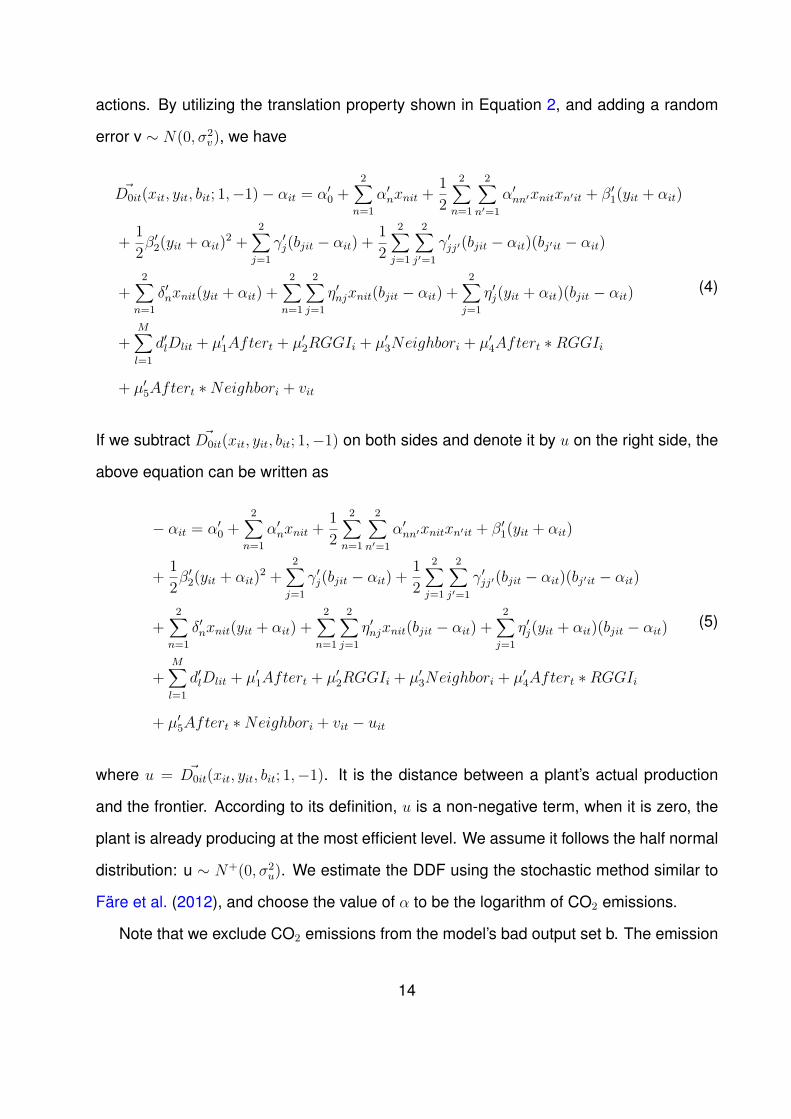
actions. By utilizing the translation property shown in Equation 2, and adding a random

error v ∼ N(0, σ2v), we have

~D0it(xit, yit, bit; 1,−1)− αit = α′0 +2∑

n=1α′nxnit + 1

2

2∑n=1

2∑n′=1

α′nn′xnitxn′it + β′1(yit + αit)

+ 12β′2(yit + αit)2 +

2∑j=1

γ′j(bjit − αit) + 12

2∑j=1

2∑j′=1

γ′jj′(bjit − αit)(bj′it − αit)

+2∑

n=1δ′nxnit(yit + αit) +

2∑n=1

2∑j=1

η′njxnit(bjit − αit) +2∑

j=1η′j(yit + αit)(bjit − αit)

+M∑l=1

d′lDlit + µ′1Aftert + µ′2RGGIi + µ′3Neighbori + µ′4Aftert ∗RGGIi

+ µ′5Aftert ∗Neighbori + vit

(4)

If we subtract ~D0it(xit, yit, bit; 1,−1) on both sides and denote it by u on the right side, the

above equation can be written as

− αit = α′0 +2∑

n=1α′nxnit + 1

2

2∑n=1

2∑n′=1

α′nn′xnitxn′it + β′1(yit + αit)

+ 12β′2(yit + αit)2 +

2∑j=1

γ′j(bjit − αit) + 12

2∑j=1

2∑j′=1

γ′jj′(bjit − αit)(bj′it − αit)

+2∑

n=1δ′nxnit(yit + αit) +

2∑n=1

2∑j=1

η′njxnit(bjit − αit) +2∑

j=1η′j(yit + αit)(bjit − αit)

+M∑l=1

d′lDlit + µ′1Aftert + µ′2RGGIi + µ′3Neighbori + µ′4Aftert ∗RGGIi

+ µ′5Aftert ∗Neighbori + vit − uit

(5)

where u = ~D0it(xit, yit, bit; 1,−1). It is the distance between a plant’s actual production

and the frontier. According to its definition, u is a non-negative term, when it is zero, the

plant is already producing at the most efficient level. We assume it follows the half normal

distribution: u ∼ N+(0, σ2u). We estimate the DDF using the stochastic method similar to

Färe et al. (2012), and choose the value of α to be the logarithm of CO2 emissions.

Note that we exclude CO2 emissions from the model’s bad output set b. The emission

14

abatement technologies for CO2, SO2, and NOx are different. The pollutants of SO2,

and NOx can be scrubbed using scrubber systems. However, CO2 can be only reduced

through reducing inputs, fuel switching, or very expensive carbon sequestration. Unlike

SO2 and NOx, there is no convincing successful end of pipe treatment to effectively abate

CO2. Our data show that CO2 and heat input are correlated with the correlation equal to

99%, indicating that CO2 is fully determined by heat input within both coal and natural gas

groups.

After estimating the model, we can calculate the plant-level technical efficiency value.

Following Battese and Coelli (1993), we define the technical efficiency of the ith plant in

year t as:

TEit = E(e−uit|vit − uit) (6)

The calculation formula can be found in Gronberg et al. (2005); note that the calculated

TE is always within [0, 1].

Data Sources

We use detailed plant-level data from U.S. Environmental Protection Agency (EPA) and

Energy Information Administration (EIA) to estimate the DDF. EPA’s Air Market Program

Data (AMPD) provides information on each power plant’s input capacity, heat input for

electricity generation, gross generation, and air emissions. EIA survey form EIA-860

collects information on individual plant’s location, ownership type, regulatory status and

NERC region code. Form EIA-923 collects data on CHP (Combined Heat and Power)

availability, prime mover type and primary fuel type. Merging all these data, we obtain an

unbalanced panel dataset that consists of 1191 fossil-fuel power plants operating in the

U.S. over a 12-year period from 2002-2013, for a total of 10,742 observations. Among

them, 3649 observations are from plants that use coal as the primary fuel, 7093 are from

natural gas plants.

15

Table 1 reports the descriptive statistics for variables used in the estimation. We fo-

cus only on coal and natural gas plants and exclude petroleum plants from the analysis.

Petroleum is usually used in electricity generation as a supplemental fuel to coal and nat-

ural gas in order to cover demand spikes. In addition, petroleum plants only account for

4% of the observations, and the impact of regulations will be small in magnitude. We only

include relatively purer coal (natural gas) plants which is defined as having more than 98%

of electricity output generated by coal (natural gas). Plants in New Jersey are special in

the sense that they participated RGGI in 2009 and withdrew at the end of year 2012. To

avoid any confusion, we drop these plants.

Table 1 shows that natural gas plants are generally much smaller in capacity than coal

plants. The average input capacity for natural gas plants is less than half of the average

for coal plants. In addition, the gross generation and heat input of a coal plant are more

than five times greater than those of a natural gas plant.

The distributions of input capacity and heat input for each fuel-type plants are shown

in Figure 1. Panel (a) shows that the input capacity for a majority of natural gas plants is

smaller than coal plants. Panel (b) shows that most natural gas plants have small heat

input.

Figure 1: Distribution of Input Capacity and Heat Input

(a) Input Capacity (b) Heat Input

16

Table 1: Plant-level Summary Statistics

Coal Natural gasVariable Unit Notation Mean or Percentage Std. Dev. Mean or Percentage Std. Dev. Source

Gross generation Million MWh y 5.61 5.04 1.01 1.59 AMPDHeat input Million MMBtu x1 55.25 48.34 8.99 13.14 AMPDInput capacity Thousand MMBtu/hr x2 10.84 9.01 4.69 4.23 AMPDCO2 Thousand Tons α 5183.82 4534.62 481.69 709.32 AMPDSO2 Thousand Tons b1 20.37 26.86 0.05 0.30 AMPDNOx Thousand Tons b2 7.72 7.84 0.21 0.56 AMPDRegulatory status Binary regulate 76.76% 46.85% EIA 860

Ownership type:Cooperative Binary owner1 9.43% 6.98% EIA 860Federally-owned Binary owner2 0.66% 0.62% EIA 860Investor-owned Binary owner3 47.22% 25.70% EIA 860Municipally-owned Binary owner4 8.00% 11.24% EIA 860Political Subdivision Binary owner5 1.67% 2.41% EIA 860Independent Power Producer Binary owner6 1.48% 1.10% EIA 860State-owned Binary owner7 11.87% 31.59% EIA 860Other Binary owner8 19.67% 20.36% EIA 860

NERC region:Florida Reliability Coordinating Council Binary nerc1 1.23% 4.38% EIA 860Midwest Reliability Organization Binary nerc2 13.07% 4.26% EIA 860Northeast Power Coordinating Council Binary nerc3 2.82% 10.53% EIA 860ReliabilityFirst Corporation Binary nerc4 32.34% 14.80% EIA 860SERC Reliability Corporation Binary nerc5 27.05% 18.16% EIA 860Southwest Power Pool, RE Binary nerc6 7.40% 10.55% EIA 860Texas Regional Entity Binary nerc7 4.41% 11.76% EIA 860Western Electricity Coordinating Council Binary nerc8 11.67% 25.56% EIA 860

Year 2009 and beyond Binary after 40.83% 48.06% EIA 860RGGI states Binary rggi 4.52% 11.24% EIA 860Neighboring states Binary neighbor 11.40% 4.27% EIA 860CHP Binary chp 0.93% 10.63% EIA 923

Prime mover type:Combined cycle-steam part Binary prime1 0.00% 0.47% EIA 923Combined cycle combustion-turbine part Binary prime2 0.00% 41.38% EIA 923Combustion (gas) turbine Binary prime3 0.00% 34.25% EIA 923Steam turbine Binary prime4 91.86% 15.87% EIA 923Other Binary prime5 8.14% 8.03% EIA 923

No. of observations 3649 7093

17

About 76.76% of coal plants are regulated by local public utilities commissions, while

only less than half of natural gas plants are so regulated. We define Pennsylvania, Vir-

ginia, West Virginia, and District of Columbia as "neighboring states" of RGGI states. In

our sample, 8.96% of total observations are from plants within RGGI states, while 6.69%

are from plants located in neighboring states. RGGI states have more natural gas plants,

while neighboring states have more coal plants. Among natural gas plants, 10.63% have

at least one CHP generator, but this number is only 0.93% for coal plants. We also include

dummy variables that indicate ownership types, NERC regions, and prime mover types

of the generator with the highest generation in one power plant. In Table 1, we list all the

notations for the variables that will be used in the model.

Figure 2 plots the number of plants over time. For the RGGI area, neighboring states

and other areas, the number of coal plants is relatively stable, and has slightly declined in

recent years, while the number of natural gas plants is increasing. It shows that, in recent

years, the newly built plants are mostly natural gas plants for all areas. Compared to other

areas, the gap between number of natural gas plants and number of coal plants is much

bigger in RGGI, indicating that RGGI relies more heavily on the cleaner energy.

Figure 3 further examines gross electricity generation by fuel type and area. The three

panels in the left column illustrate the aggregate generation and show that the use of

natural gas in all three areas increases during the sample period. Generation by natural

gas is even higher than by coal in the RGGI area after 2006, while it is much lower

than coal generation in other two areas. Over time, the aggregate gross generation from

coal plants has declined in all three areas. The three panels in the right column plot

the average gross generation over plants. In the RGGI area, although the aggregate

generation by natural gas plants is much higher than that of coal plants, the average

generation by natural gas plants is still lower than that of coal plants, with a slight increase

over years because there are many more natural gas power plants. Average generation

by natural gas plants increases slightly in neighboring states and other areas as well. The

18

Figure 2: Number of Plants

(a) RGGI

(b) Neighbor

(c) Other

19

Figure 3: Gross Generation by Fuel Type and Area

(a) Aggregate - RGGI (b) Average - RGGI

(c) Aggregate - Neighbor (d) Average - Neighbor

(e) Aggregate - Other (f) Average - Other

20

average generation by coal plants shows a declining trend in the RGGI and neighboring

area, but remains stable in other areas. As natural gas plants are very different from coal

plants, in the next section, we divide all plants into coal plants and natural gas plants, and

then estimate each group’s DDF model.

Determinants of Plant-level Technical Efficiency

We estimate the DDF model (Equation 1) using Equation 5 for coal and natural gas plants

separately. In Equation 5, uit measures the distance to the production frontier, which is the

maximum possible simultaneous increase in good outputs and decrease in bad outputs

given the amount of inputs. A negative coefficient indicates a positive impact on efficiency.

The estimates are presented in Table 2. Using the notation in Table 1, y is the electricity

generation, and x1 and x2 are heat input and input capacity, respectively. The bad outputs,

b1 and b2 are the amount of SO2 and NOx, respectively. Note that we exclude SO2 when

estimating the model for natural gas plants due to the extremely low sulfur content of

natural gas.7 The variable "after" indicates the year dummy for the RGGI policy. For year

2009 and beyond, after = 1, otherwise 0. It captures any change that occurred in 2009

over all geographic areas. If the plants are RGGI power plants, rggi = 1, and if they are

in the states neighboring the RGGI area, neighbor = 1. We also include after ∗ rggi and

after ∗ neighbor to measure the impact of RGGI policies on distance for plants located in

RGGI and neighboring states. Table 2 shows that the coefficients for after are statistically

significant and negative for natural gas plants, but not significant for coal plants. This

indicates that natural gas plants became more efficient after year 2009 due to reasons

other than RGGI policies, and no such change is found for coal plants. The significant

coefficient for RGGI in the result implies that the efficiency of coal plants in the RGGI

area is lower than plants in other areas.7In 2012, the average SO2 emission intensity of a natural gas power plant with combined cycle was

0.2% of that of a coal power plant.

21

Table 2: Estimates of the Directional Distance Function ModelVariable Coal Natural gas Variable Coal Natural gasy -0.921∗∗∗ -0.844∗∗∗ owner1 0.004 -0.016∗∗

(0.015) (0.010) (0.012) (0.007)x1 0.069∗∗∗ 0.058∗∗∗ owner2 0.072∗ 0.031∗

(0.002) (0.006) (0.039) (0.020)x2 -0.044∗∗∗ -0.011∗∗∗ owner3 0.003 -0.006

(0.007) (0.002) (0.008) (0.006)b1 2.530b owner4 -0.009 -0.023∗∗∗

(1.730) (0.012) (0.007)b2 -2.340b -0.274∗∗∗a owner5 -0.025 -0.021∗

(6.430) (0.028) (0.020) (0.011)y2 0.039∗∗∗ 0.038∗∗∗ owner6 -0.011 -0.013

(0.005) (0.003) (0.019) (0.009)x2

1 0.229∗∗∗a -0.691∗∗∗a owner7 -0.032∗∗∗ 0.019∗∗∗

(0.075) (0.142) (0.012) (0.006)x2

2 6.660b 0.243∗a nerc1 0.063∗∗∗ -0.014(36.600) (0.133) (0.020) (0.015)

b21 0.002c nerc2 0.014 0.015∗∗∗

(0.005) (0.011) (0.005)b2

2 -0.109c 5.160c nerc3 0.011 -0.016(0.076) (4.770) (0.025) (0.019)

x1x2 -1.565∗∗∗a 1.128∗∗∗a nerc4 0.059∗∗∗ -0.011(0.286) (0.294) (0.011) (0.007)

b1b2 0.037c nerc5 0.056∗∗∗ 0.003(0.029) (0.009) (0.006)

x1b1 -0.050b nerc6 -0.011 0.012∗∗

(0.055) (0.010) (0.006)x1b2 0.210b -2.760b nerc7 0.053∗∗∗ -0.017∗∗

(0.164) (1.900) (0.015) (0.008)x2b1 -0.118∗∗∗b prime1 -0.046∗∗

(0.040) (0.021)x2b2 0.100b -1.400b prime2 0.001

(0.168) (1.480) (0.008)yx1 -0.006∗∗∗ 0.080a prime3 -0.008

(0.001) (1.155) (0.009)yx2 0.014∗∗∗ -0.005∗∗∗ prime4 -0.009 -0.044∗∗∗

(0.002) (0.001) (0.015) (0.011)yb1 0.294b after 0.009 -0.013∗∗

(0.468) 0.010 (0.007)yb2 -1.170b 0.045∗∗∗a rggi 0.054∗∗∗ 0.005

(1.430) (0.011) (0.021) (0.018)t -0.001 0.016∗∗∗ neighbor 0.028∗∗ 0.024∗

(0.004) (0.003) (0.013) (0.013)chp -0.159∗∗∗ -0.030∗∗∗ after ∗ rggi 0.013 -0.011

(0.025) (0.010) (0.023) (0.012)regulate 0.014 0.009∗ after ∗ neighbor 0.037∗∗ 0.055

(0.010) (0.006) (0.015) (0.039)t2 0.443a -0.669∗∗∗a constant -0.071∗∗∗ 0.179∗∗∗

(0.302) (0.196) (0.024) (0.013)No. of observations 3649 7093

a b c Coefficients are multiplied by 103, 106, 109, respectively.Robust standard errors in parentheses. ***: p < 1%, **: p < 5%, *: p < 10%.

22

We are particularly interested in the coefficient of after ∗ rggi as it is the diff-in-diff

estimator representing the impact of RGGI policies on the directional distance. The results

show that the coefficients of after ∗ rggi are statistically insignificant for both fuel groups,

meaning there is no clear evidence of RGGI undermining technical efficiency for both fuel

types of plants in the RGGI area. The coefficients for after ∗ neighbor show that there

is no policy impact on natural gas plants’ technical efficiency within neighboring states.

However, the policy decreases the technical efficiency for coal plants within neighboring

states. A likely explanation is that since the neighboring states are not regulated by the

RGGI policy, less efficient plants in neighboring states could produce more than usual

due to a spillover effect, then leading to a decreased level of technical efficiency.

However, the magnitude of the spillover effect is found quite small. After estimating

the DDF model, we can calculate TE according to Equation 6. We can then calculate the

average TE for the coal plants within neighboring states and compare it to the TE value

of setting the coefficient for after ∗ neighbor to be zero (no policy scenario). We find that

with policy enforcement, the average TE for the coal plants in the neighboring states after

2009 is 89.35%, while the average without RGGI policy is 90.67%. Therefore the RGGI

policy reduces the technical efficiency for the coal plants in the neighboring states with a

very small amount (1.48%).

Industry Dynamics

Our major finding in the previous section is that RGGI policies reduce TE of neighboring

coal plants, and no such impact is found for both types of RGGI plants and natural gas

plants in neighboring states. Note that the analysis is at the plant level. In this section, we

analyze the change of efficiency at the industry level.

We start by comparing TE averages. Across all areas and years, the average TE for

coal and natural gas plants are 88.70% and 83.14%, respectively. These values suggest

23

that, overall, the power plants are quite efficient. These values are also very similar to the

findings in Hiebert (2002). To examine more details of industrial TE, Figure 4 plots the

average TE scores by year and area. Panel (a) shows that the average TE for coal plants

increases slightly for both RGGI and other areas over time. However, the change in TE

for neighboring coal plants is minimal. Overall, efficiency is very stable and similar in all

three areas. It is between 85% and 92% across all areas and in all years. Like we have

pointed out in the previous section, although the RGGI policy lowers TE of neighboring

coal plants as indicated by Table 1, the change is small and not obvious by examining the

graph.

Figure 4: Average Technical Efficiency by Fuel Type

(a) Coal

(b) Natural Gas

24

Panel (b) in Figure 4 illustrates the changes in TE for natural gas plants. In general,

natural gas plants are less efficient than coal plants. Over time, the average technical

efficiency of natural gas plants in RGGI states and other areas is stable. In contrast,

neighboring natural gas plants show a slight decline in technical efficiency after 2009. The

impact might be due to factors other than RGGI policies, for example, other production

process changes or a structural change through entry or exit, which will be analyzed later.

To clearly show the magnitude of the change, we calculate the average TE for two

periods: 2002-2008 and 2009-2013. The result is reported in Table 3. We find that,

compared to the 2002-2008 average, the 2009-2013 average TE for coal plants increases

by 2.45% in the RGGI area, 0.17% in neighboring states and 1.26% in other areas. Unlike

coal plants in RGGI and other areas, coal plants in neighboring states do not experience

a clear increase in TE. For natural gas plants, the changes vary across areas. The 2009-

2013 average TE increases by 1.18% in other areas, but decreases by 0.93% and 3.57%

in RGGI and neighboring states, respectively. Although the TE of neighboring natural gas

plants decreases more than natural gas plants in other two areas, it is not attributed to

RGGI as indicated in Table 2.

Table 3: Change of Industrial Technical Efficiency

Fuel Type Area Average TE Average TE Change(2002-2008) (2009-2013)

Coal RGGI 0.8771 0.8986 +2.45%Coal Neighbor 0.8920 0.8935 +0.17%Coal Other 0.8818 0.8929 +1.26%Natural Gas RGGI 0.8250 0.8173 -0.93%Natural Gas Neighbor 0.8356 0.8058 -3.57%Natural Gas Other 0.8288 0.8386 +1.18%

Fuel Type Area With Policy Average TE No Policy Average TE Change(2009-2013) (2009-2013)

Coal Neighbor 0.8935 0.9067 +1.48%

The impact of RGGI regulations on TE is of particular interest. As the impact is in-

cluded in the DDF model (Table 2), we are able to calculate the TE level when there is

no RGGI program. The results from the DDF show that the RGGI program affects only

25

neighboring coal plants (which we call it a spillover effect in the previous section), so we

compare the TE with and without RGGI regulations for this group. We have already cal-

culated the TE values for the scenario with the RGGI program. For the scenario without

RGGI, we set the coefficient of after ∗neighbor to be 0 for natural gas plants, and recom-

pute TE. Figure 5 illustrates the counterfactual analysis. The dashed line is with policy in

reality, while the solid line represents the counterfactual scenario when there is no regu-

lation. The trend clearly shows that without policy, the TE level for neighboring coal plants

is higher than it is with the policy. In fact, the RGGI policy enforcement leads to a 1.48%

decline in the 2009-2013 average TE for coal plants in neighboring states. This has been

mentioned in the previous section and also reported in Table 3.

Figure 5: Neighbor Coal Plants: With and Without Regulation

To explore how the plant-level TE changes structurally, we plot the distributions of TE

in Figure 6. As shown in Panel (a) of this figure, for coal plants in the RGGI area, the

distribution shifts rightwards after year 2009, with thinner tails in the neighborhood of low

technical efficiency scores. Coal plants in neighboring states and other areas have higher

peaks after 2009, but the overall increase is not as significant as that of RGGI coal plants.

Panel (b) shows that the average TE of natural gas plants in neighboring states has a

26

notable decrease after 2009, no such evidence is found for the other two groups. All

features found in Figure 6 are consistent with those in Figure 4 and Table 3.

Figure 6: Kernel Density of TE: Before and After 2009

(a) Coal (b) Natural Gas

Two potential mechanisms can explain the changes of the average TE. One is a plant-

level technical efficiency change through a change in production process, e.g. changes

in energy efficiency, extra input for reducing emissions or less flexibility in production.

The other is a structural change through plants’ entry and exit. To isolate these two

27

mechanisms, we separate the entry and exit plants from other plants and examine their

TE separately. In our data, the number of coal plants declined over time, while the number

of natural gas plants increased tremendously in the RGGI area. In fact, there was rarely

entry of coal plants and rarely exit of natural gas power plants. In the RGGI area, only one

coal plant entered and one natural gas plant exited after 2009. Therefore, for coal plants,

we compare TE of exiting and remaining plants, while for natural gas plants, we compare

entry and remaining plants. Figure 7 presents the comparison for RGGI plants.

Figure 7: Kernel Density of TE for RGGI Plants: Change of Incumbent Plants and Entryand Exit

(a) Incumbent Coal Plants: Before and After2009

(b) Incumbent Natural Gas Plants: Beforeand After 2009

(c) Exit and Incumbent Coal Plants: Before2009

(d) Entry and Incumbent Natural Gas Plants:After 2009

For coal plants, we define exit plants as those that produced before 2009, and shut

down after 2009. We call the remaining plants incumbent plants. Panel (a) illustrates the

TE change excluding exit plants and only for incumbent ones, and Panel (c) compares

28

the incumbent and exit plants. According to Panel (a), incumbent plants became more

efficient after 2009. For exit plants, we can only see their TE value before the RGGI

program. Panel (c) shows that exit plants are relatively less efficient than incumbent

ones. Before 2009, the average TE for exit coal plants in the RGGI area is 86.68%, which

is lower than that of the incumbent ones (88.25%). Combining these two effects from

Panel (a) and (c), the coal plants became more efficient after 2009, which is consistent

with the result in Panel (a) of Figure 6.

With regard to natural gas plants, we define entry plants as those that operated after

2009. As shown in Panel (b), incumbent plants have a similar TE distribution before and

after 2009. Panel (d) plots the comparison of entry and incumbent plants, which again

shows similarity in TE between new entry plants and incumbent ones. But in fact, the

entry plants are slightly more efficient (TE is 84.54%) than the incumbent ones (TE is

80.70%) after 2009. Again, these two effects together contribute to the outcome that

technical efficiency levels of RGGI natural gas plants did not change much after 2009.

So far, we have presented three interrelated terms: 1) average TE, 2) entry or exit of

power plants, and 3) RGGI policy impact captured in the DDF model. As the RGGI policy

impact captured in the DDF is at the plant level, it does not capture the effect of entry or

exit of power plants. Therefore 1) is a combination of 2) and 3) and other factors, and is

not necessarily caused by RGGI policies. The before and after increase is due to multiple

reasons. For example, it could be due to many other variables in the DDF model including

time trend, other policies etc. (Table 2) and the RGGI regime is only one of the causes. It

could also be due to entry or exit of power plants.

Concluding Remarks

In this paper, we employ DDF estimation to investigate changes in technical efficiency of

fossil fuel plants due to the implementation of the RGGI program. With detailed plant-

29

level data from coal and natural gas plants in all states, we find no evidence that the

RGGI program changes the technical efficiency of both fuel types of power plants in the

RGGI area. For RGGI coal plants, less efficient plants exited the market, while more ef-

ficient natural gas plants entered compared to the incumbent plants. We also consider

the possibility that the RGGI policy might affect plants in neighboring states through in-

terconnected market, and find that the RGGI regulation leads to a 1.48% decline in the

average technical efficiency for coal plants within neighboring states during 2009-2013

using a counterfactual analysis.

Although we find minor impacts of carbon emission regulation on the technical ef-

ficiency of power plants, they do not undermine the value of our study. The findings

remove the policymakers’ concern about a sudden drop of technical efficiency at least at

the current stage. However, our results should be viewed as being short run and they do

not necessarily eliminate the impacts in the long run. As climate change becomes a more

and more important international issue, and the concern over the economic burdens be-

comes one of the biggest hurdles that prevent countries from taking aggressive actions,

more research is called for in this area.

30

Chapter Two

Carbon Prices and Fuel Switching: A Quasi-experiment in Electricity Markets

Ling Huang

University of Connecticut

Yishu Zhou

University of Connecticut

Abstract

Within the Pennsylvania-New Jersey-Maryland (PJM) electricity market, Delaware and

Maryland participate in the Regional Greenhouse Gas Initiative (RGGI) but other states do

not, providing a quasi-experiment setting to study the effectiveness of the RGGI program.

Using a difference-in-difference framework, we find that overall the RGGI program leads

to 7.72 million short tons of CO2 reduction per year in Delaware and Maryland, or about

34.36% of the average total annual emissions in these two states from 2009 to 2013.

We find little evidence that utilities adjust their capacities within five years after program

implementation except natural gas-only utilities. All utilities respond to the program by

decreasing their heat input per capacity even including natural gas utilities. Counter-

intuitively, the reduction is mainly achieved through reduction of coal and natural gas input

and emission leakage instead of fuel switching from coal to natural gas or from fossil fuel

(coal and natural gas) to non-fossil fuel. The results suggest that the power utilities do

respond to the emission trading program with current carbon prices, but tremendous fuel

switching did not occur before 2013 due to the program as it is less costly to leak the

emissions under the regional regime.

Keywords: Carbon Emission Market, RGGI

31

Introduction

The U.S. Electric power sector accounts for 2,122 million short tons of carbon dioxide

(CO2) emissions in 2015, or about 37% of the total U.S. energy-related CO2 emissions.

8 To address the climate change issues, the power sector is critical. However, the power

sector appears to have a limited option to reduce CO2: phasing out coal power plants

and replacing with cleaner plants, i.e. fuel switching in a general sense. It is far from

easy, though, since emission reduction could force heavy economic burden on the exist-

ing fossil-duel power plants. Therefore, the Clean Power Plan, as the first-ever national

standard to reduce CO2 from power plants, has encountered very strong opposition since

its announcement on August 3, 2015. 9 Understanding fuel switching for fossil-duel power

plants is essential to the success of any future program targeting at reducing CO2.

The Regional Greenhouse Gas Initiative (RGGI) is the first cooperative effort in the

U.S. to reduce CO2 emissions among the states of Connecticut, Delaware, Maine, Mary-

land, Massachusetts, New Hampshire, New York, Rhode Island, and Vermont, specifically

in the electric power sector. 10 RGGI aims to stabilize and then reduce CO2 emissions

within the signatory states. Regulated sources of emissions are fossil fuel-fired power

plants with a capacity of 25 MW or greater, located within the RGGI states. RGGI was for-

mally initiated in 2003 and compliance started on January 1, 2009. 11 According to RGGI8EIA data: http://www.eia.gov/tools/faqs/faq.cfm?id=77&t=11.9The U.S. Supreme Court granted a stay on the implementation of Clean Power Plan because of cases

filed by more than two dozen states and numerous industry groups.10Globally, the carbon emission trading market has been increasing in recent years. After the implementa-

tion of the European Union Emissions Trading Scheme (EU ETS), several domestic and regional initiativesemerged in developed and developing countries including the RGGI (Kossoy and Guigon, 2012). Currently,the United States has altogether three systems related to GHG emission trading: the RGGI, the California,Qubec and the Western Climate Initiative, and the Chicago Climate Exchange (CCX). The first two aremandatory schemes, while the CCX is operated on a voluntary base.Unlike traditional harmful pollutantsexplicitly regulated by the Clean Air Act (SO2 and NOx), CO2 emissions are a new pollution source thatraises many new questions. Reduction of CO2 is regulated under section 111(d) of Clean Air Act whichcovers other unnamed potential pollutants. These pioneering programs can provide very helpful guidelinesfor the future carbon markets in the U.S.

11Every control period lasts three years, and, at the end of the third year of a control period, each regu-lated plant is required to hold one allowance for each ton of CO2 emitted. Unused allowances do not expireand can be banked for future years. If a plant violates the rule, it needs to surrender a number of allowancesequal to three times the number of its excess emissions.

32

(2014), average CO2 emissions from 2010-2012 in RGGI states decreased by 25.4%,

compared with the average from 2006-2008. In addition, the CO2 emission rate (pounds

of CO2 per megawatt hour) dropped by 16.7% during the same period. However, multiple

factors could have triggered the emission decrease. Lower natural gas prices, decrease

of demand or increase of renewable capacity could all lead to CO2 emission reduction.

This paper studies whether the RGGI program leads to the emission reduction.

There are five major ways for fossil-fuel power plants under the system of RGGI to

reduce CO2. The first one is switching to fuel with lower carbon content. 12 Changing from

coal to natural gas, for instance, can reduces a power plant’s carbon emissions by 40-60%

per megawatt hour (Mwh) taking into consideration of efficiency loss (CCES, 2013). The

second option is to switch from fossil fuel to non-fossil fuel. The third option is to improve

energy efficiency during electricity generation. This would include using more efficient

electrical appliances and improvement of technology (e.g. switching to a combined heat

and power system). The fourth method is to sponsor CO2 offset projects, including carbon

capture and sequestration, emission reduction in the building and agriculture sector, etc.

13 The fifth method is to shift the production to non-RGGI areas. Consequently, it causes

emission leakage. Among all these five methods, energy efficiency improvement and

offset projects require much more technological advancement, therefore fuel switching

and emission leakage are the main focus of this paper.

The RGGI program in the Pennsylvania-New Jersey-Maryland (PJM) electricity market

provides a perfect quasi-experiment to study the fuel switching behavior. Within the PJM

territory, Delaware and Maryland participate in the RGGI. Electric utilities from these two

states form the treatment group in the quasi-experiment. 14 Ohio, Pennsylvania, Virginia

and West Virginia, part of Illinois, Indiana, North Carolina and Kentucky are in the PJM12Per million BTU of energy, coal emits around 215 pounds, oil emits 160 pounds and natural gas emits

117 pounds of CO2.13See http://www.rggi.org/market/offsets.14An electric utility is the operating power generation unit, which can have multiple power plants and a

power plant can have multiple generators.

33

market but do not participate in the RGGI. The electric utilities from these states are

treated as the control group. Using a panel data from 2002-2013, we use a difference-in-

difference (DID) framework to isolate the impact of the RGGI program.

Our empirical results show that the RGGI program leads to 7.72 million short tons

of CO2 reduction per year in Delaware and Maryland, or about 34.36% of the average

total annual emissions in these two states from 2009 to 2013. Natural gas-only utilities

increase 5.01% emissions of their own total emissions due to the program through long-

term capacity investment, and decrease emissions by 42.26% through reducing short-

term heat input per capacity (hereafter, called utilization rate). Coal-only utilities, natural

gas capacities within the flexible utilities (with both natural gas and coal capacities) and

coal capacities within the flexible utilities decrease CO2 reduction by 20.34%, 27.14%

and 38.69% of their own emissions due to the program respectively, all through reduction

in utilization rate. The results suggest that the compliance strategies adopted by the

flexible and non-flexible utilities are similar. We implement multiple robustness checks

and confirm that our results hold under different specifications.

Another key concern we need to consider is emission leakage. Emission leakage

refers to emissions shifting outside the jurisdictional area, driven by the enforced emission

costs, which could be substantial and misleading when evaluating the effectiveness of car-

bon trading programs (Cullenward and Wara, 2014; Newell et al., 2014). Interconnected

grid network makes electricity transmission (import and/or export) possible between RGGI

and adjacent areas. Potentially, it is possible that RGGI increases the import of electricity

from non-RGGI areas. In this case, it would appear that emissions in the RGGI area are

reduced, while national emissions stay the same or even increase. We consolidate the

import data for Maryland and Delaware and find that the import did increase significantly

after 2009. In addition, the power generation excluding natural gas and coal generation in

Maryland and Delaware did not change after 2009. The results suggest that the reduction

of coal input has not been replaced by non-fossil sources. Instead, it was covered by

34

leaking the emissions to non-RGGI areas.

We compare our results to studies in the literature. Swinton (1998) estimates the

shadow price of SO2 emissions by modeling the joint production of electricity and sulfur

dioxide. He finds that fuel-switching can also significantly reduce emissions in the short

run. Linn et al. (2014a) examine the operation of coal-fired generating units and find that

a 10% increase in coal prices leads to a 0.2 to 0.5% decrease in heat rate. McKibbin et al.

(2014) compare the effects of emission reduction programs imposed on the power sector

only and economy-wide, and find that the power-sector-only approach requires a carbon

price that is almost twice the economy-wide carbon price to achieve the same cumulative

emission reduction. There is no clear evidence that pollution controls on the electric power

sector will drive up CO2 emissions outside this sector. Hitaj and Stocking (2014) find that

the U.S. SO2 allowance prices did not reflect marginal abatement costs in the early years

after implementation. In terms of reduction reasons, Ellerman and Montero (1998) find

that rail rates for shipping low-sulfur coal, rather than the 1990 Clean Air Act Amendments,

are the principal reason why sulfur dioxide emissions by electric utilities declined from

1985 to 1993. Murray et al. (2014) specifically examine the RGGI impact on CO2 reduction

and find that the emissions in the whole RGGI region would have been 24% higher without

the program. Our study contributes to the literature by specifically estimating the fuel

switching behavior to carbon price signals and examining how emissions are reduced at

a micro-level. In addition, our studies trace the emission reduction back to individual utility

level and take advantage of the quasi-experiment setting.

This paper also contributes to the literature on emission trading programs. A well-

designed emission trading program has been learnt that it can effectively reduce air pol-

lution (Joskow et al., 1998; Stavins, 1998; Ellerman et al., 2000; Stavins, 2003; Sterner,

2003). Many studies examine these programs from different perspectives. For example,

Bovenberg et al. (2005) examine the efficiency costs of choosing particular environmen-

tal permits and taxes. Rubin (1996) develops a framework for modeling emission trading,

35

banking, and borrowing, and uses optimal control theory to derive optimal time paths for

emissions by firms. Subramanian et al. (2007) characterize firms’ compliance strategies

under an emission cap and trade program with a three-stage model of structural deci-

sions on abatement, permit auction, and production. Hart and Ahuja (1996) and Smale

et al. (2006) examine the impact of emission regulations on firm performance. Joskow et

al. (1998) evaluate the economic impacts of the RGGI on ten Northeast and Mid-Atlantic

States and find that the program expenditures benefit the region’s economy. Ruth et al.

(2008) study the economic impact of participation in RGGI on the state of Maryland and

find little net impact. Our paper examines the effectiveness of emission trading programs

from the perspective of firm production decisions.

In addition to the literature on cap and trade program evaluation, our study also con-

tributes to the literature investigating which factors can determine emissions. Vollebergh

et al. (2009) and Holtz-Eakin and Selden (1995) use country-level panel data to regress

the amount of CO2 or/and SO2 emissions on variables such as income and per capita

GDP. Auffhammer and Carson (2008) forecast China’s CO2 emissions using province-

level data, and concluded that emissions in China are unlikely to decrease in the near

future unless substantial changes in energy policies occur. Cole et al. (2013) explore

the factors influencing firms’ CO2 emissions with firm-level data from Japan and found

emissions among firms are spatially correlated. Our study takes the perspective of firm

production and focuses on the input function and examines what factors determine CO2

emissions.

The rest of the paper is organized as follows. Section 2 describes the methodology,

followed by Section 3, which presents the data. Model results and robustness check are

in Section 4 and 5. Section 6 presents the emission reduction quantification and Our

conclusions are finally presented in Section 7.

36

Methodology

There are three fossil fuel types of utilities: coal, natural gas and Petroleum. Since

petroleum is not frequently used and counts only a very small fraction of total heat gen-

erated from fossil fuel combustion, we hence focus on fuel switching between natural gas

and coal among fossil fuel utilities. We define fuel switching between natural gas and

coal as replacing coal heat input by natural gas. It can take multiple hypothetical forms.

At the industry level, if natural gas utilities increase capacity and inputs, while coal util-

ities decrease capacity and inputs, the relative fuel inputs structure of the industry can

change. It is also possible that more natural gas utilities enter the market and more coal

utilities exit. At the utility level, a utility can directly increase their natural gas inputs rel-

ative to coal inputs in the short term. In the long term, they can invest more natural gas

capacity. As different types of utilities have different forms of fuel switching, we divide the

utilities into three excludable categories: 1) non-flexible always-staying utilities; 2) flexible

always-staying utilities; and 3) entry and exit utilities. Entry and exit of utilities can alter

the capacity structure in terms of fuel types. Those utilities who do not enter or exit the

market are always-staying utilities. Among the always-staying utilities, we define flexible

utilities as those having both coal and natural gas power plants. In fact, fuel switching

can occur even at the generator level: some generators can use multiple types of fuel.

15 Non-flexible utilities are natural gas-only and coal-only utilities. 16 In the following, we

analyze response to the RGGI program by each category separately.

For a non-flexible always-staying utility, its heat input can be written as:

Iitx = Zitx ∗Iitx

Zitx

for x = c, n (7)

15See http://www.eia.gov/tools/faqs/faq.cfm?id=65&t=3. For a generator that can use both fuel types,we double count its capacity for natural gas capacity and coal capacity, but count only once for the totalcapacity.

16In our data, some utilities are non-flexible always-staying utilities in some years and flexible always-staying utilities in other years. We categorize them into flexible always-staying utilities.

37

in which Iitx is utility i’s heat input at time t and Z is its capacity. The notation x indicates

its fuel type. While x = n indicates a natural gas utility, x = c indicates a coal utility.

Therefore, the change of heat input can be written as:

4Iitx = 4Zitx ∗Iitx

Zitx

+ Zitx ∗ 4Iitx

Zitx

= 4Zitx ∗ Uitx + Zitx ∗ 4Uitx (8)

Equation 8 states that the change of heat input can be decomposed into a long-term

capacity adjustment 4Zitx and a change in the utilization rate Uitx. Later, we need to

examine whether the RGGI program has led to changes in these two terms.

For a flexible always-staying utility, since it has both natural gas and coal power plants,

a direct way is to treat its natural gas and coal capacities as two separate units and

examine their capacity adjustment and heat input decisions separately. However, within

one single utility, the decisions of capacity adjustment and input decisions of natural gas

and coal are inter-correlated and not independent. Therefore, we write its inputs of natural

gas and coal as the following:

Iitc = (Zitn + Zitc) ∗ Zitc

Zitn+Zitc∗ Iitc

Zitc

Iitn = (Zitn + Zitc) ∗ Zitn

Zitn+Zitc∗ Iitn

Zitn

(9)

in which

Zitx% = Zitx

Zitc + Zitn

for x = c, n

Again, we call Iitc

Zitcas Uitc. Then we can write down the change of heat inputs as:

4Iitc = 4(Zitn + Zitc) ∗ Zitc%Uitc + (Zitn + Zitc) ∗ 4Zitc%Uitc + (Zitn + Zitc) ∗ Zitc%4 Uitc

4Iitn = 4(Zitn + Zitc) ∗ Zitn%Uitn + (Zitn + Zitc) ∗ 4Zitn%Uitn + (Zitn + Zitc) ∗ Zitn%4 Uitn

(10)

Differently from coal-only and natural gas-only utilities, change of inputs can be decom-

38

posed to change of total capacity, percentange change of each fuel type of capacity and

utilization rate. Using this method, we examine four key changes: 4(Zitc + Zitc), 4Zitn%,

4Uitc and 4Uitn.

For entry and exit utilities, we also start with examining their capacity change. We find

that their capacity change is a very small amount. We therefore ignore the impact of the

RGGI program on this category of utilities.

Figure 8: PJM territory served and RGGI

Note: Currently, Connecticut, Delaware, Maine, Maryland, Massachusetts, New Hamp-shire, New York, Rhode Island, and Vermont are in RGGI, in which Delaware and Mary-land are in the PJM territory. Other states in PJM but not regulated by PJM that we includein our analysis are Ohio, Pennsylvania, Virginia and West Virginia, part of Illinois, Indiana,North Carolina and Kentucky.

As noted in the Introduction, we take the advantage of a quasi-experimental setting.

Figure 8 describes the quasi-experiment. Currently, Connecticut, Delaware, Maine, Mary-

39

land, Massachusetts, New Hampshire, New York, Rhode Island, and Vermont participate

in the RGGI. Within the PJM territory, Delaware and Maryland are regulated by the pro-

gram. Utilities from these two states serve as the treatment group. Other states in the

PJM market but not regulated by the RGGI that we include in our analysis are Ohio,

Pennsylvania, Virginia and West Virginia, part of Illinois, Indiana, North Carolina and

Kentucky. Utilities from these states serve as the control group. In other words, within

the Pennsylvania-New Jersey-Maryland (PJM) market, power utilities in Maryland and

Delaware have to purchase CO2 allowances after 2009 under RGGI, while utilities in

other states are free to emit CO2. New Jersey is also in PJM, but they withdrew from the

program at the end of year 2011. So we exclude New Jersey from our analysis.

With the quasi-experimental setting and panel data, we apply a simple DID method

to isolate the impact of RGGI program on each category of utilites. For the non-flexible

always-staying utilities, the corresponding reduced DID regression can be written as:

Yitx =β0 + β1Pitx + β2Pet + β3trendyear + β4Demandt + β5Sit

+ β6Afteryear + β7Afteryear ∗RGGIi + αi + εit for x = c, n

(11)

in which

Yitx = Zitx or Uitx

where Yitx is the dependent variable and it could be Zitx or Uitx. Zitx is the capacity of

natural gas or coal of ith utility in time t and Uitx is the utilization rate. When estimating the

capacity model, the data is yearly, and when estimating the utilization rate model, the data

is monthly. So the time t is different for these two models. For the utilization rate model,

monthly dummies from January to December are added to control for seasonal patterns.

The term Pitx is fuel price across individual utility and time and Pet is electricity price at

time t. The term trend is the yearly time trend. We also include PJM area’s total demand

and regard it exogenous. With higher electricity demand, more natural gas plants need

40

to be brought up online, to serve the peak demand along with the base load coal plants,

thus increasing natural gas usage. The term αi is the time-invariant individual utility fixed

effect and Sit is time-variant characteristics of utilities including capacity, combined heat

and power (CHP) availability and age. After is a dummy variable, which equals to 1 for

the years after 2009 and 0 otherwise. It captures any change before and after 2009 for

the whole PJM area. Dummy of RGGI captures regional differences of natural gas usage

percentage. If the utility is located in the RGGI area, RGGI is equal to 1, 0 otherwise.

The term Afterit ∗ RGGIi is the treatment. After controlling for year 2009 and individual

fixed effects, the coefficient, β7, is expected to reflect the impact of the RGGI program on

Yitx.

For the flexible always-staying utilities, a few things need to be altered:

Yitx =β0 + β1Pitn + β2Pitc + β3Pet + β4trendyear + β5Demandt + β6Sit

+ β7Afteryear + β8Afteryear ∗RGGIi + αi + εit for x = c, n

(12)

in which

Yitx = Zitc + Zitc, logit(Zitc%), Uitc or Uitn

The dependent variables are Zitc + Zitc, logit(Zitc%), Uitc and Uitn. Zitc + Zitc is the total

capacity including natural gas and coal. Zitc% is the percentage of capacity from natural

gas. Since it is a percentage value ranging from 0 to 1, we use its logit transformation.

Uitc and Uitn are the utilization rate of natural gas and coal, respectively. In Equation 12,

we use both fuel prices pitn and pitc as the explanatory variables, which can be considered

by a flexible utility simultaneously.

41

Data

Three major datasets are used. The first one is EIA 860, which collects generator-level

information, including whether the generator has a co-fire function, its capacity, operation

age, fuel type, whether it has a combined heat and power system, region, etc. The sec-

ond dataset is EIA 923, which contains detailed electricity generation data, including heat

content of fuels, quantity of fuels, prime mover, net generation, heat content/fuel cost by

contract, contract type, contract expiration date, fuel cost, abatement expense and abate-

ment investment for all pollution, etc. The third dataset is the Emissions & Generation

Resource Integrated Database (eGRID), provided by the U.S. Environmental Protection

Agency (EPA), which is the main data source on CO2 emissions. Plant identification infor-

mation from PJM’s website is used to match PJM plants with the above three datasets.17

We also acquire state-level fuel costs, demand and generation from EIA’s Electric Power

Monthly issues.18 The data consist of 196 fossil fuel electric facilities from 124 utilities

operating in the PJM area over the 144-month period from 2002-2013, for a total of 14940

observations.19 Because of entry and exit, not every utility appears in all the 144 months.

The average number of observations per utility is 120.5.

Table 4 reports summary statistics of variables used in regressions and data sources.

Fuel prices are averaged over monthly transactions, thus vary across utilities and time.

If a utility’s fuel prices are missing, we replace them with the monthly average state fuel

prices reported in EIA’s Electric Power Monthly issues. Figure 9 plots the average monthly

natural gas price and coal price. Comparing to coal, natural gas has a much higher price

per unit of heat input, about three times as expensive as coal on average. Our data also

show that coal is the dominant fossil fuel in this industry: heat input by coal is about 9

times as high as heat input by natural gas. This is due to the reason that coal plants are17See http://www.pjm.com/documents/reports/eia-reports.aspx.18See http://www.eia.gov/electricity/monthly/.19If an utility has plants in multiple states, we treat them as separate utilities, as they face distinct state-

level regulation policies.

42

often used to serve base load and operate almost constantly. The average coal capacity

is only 240 MW more than the natural gas capacity, indicating a significant potential for

fuel switching even without new investment. We weight the age of generators from the

same utility by capacity to get a utility’s weighted age, and the average is 20 years. For the

utilities we include in our sample, the RGGI regulated areas are Delaware and Maryland,

which encompasses 11.49% of the total electricity generation by natural gas and coal.

Table 4: Summary Statistics

Variables Mean Std. Dev. Source

Natural gas price (¢/MMBtu) 630.23 247.61 EIA 923Coal price (¢/MMBtu) 208.12 70.99 EIA 923Heat input by coal (Million MMBtu) 2.76 5.70 EIA 923Heat input by natural gas (Million MMBtu) 0.32 0.90 EIA 923Dummy of CHP availability (%) 25.62 EIA 923Dummy of after policy year 2009 (%) 42.17 EIA 923

Age (year) 20.44 14.49 EIA 860Coal Capacity (MW) 628.70 1256.03 EIA 860Natural gas Capacity (MW) 390.28 619.68 EIA 860Ownership-Joint (%) 7.95 EIA 860Ownership-Single (%) 74.78 EIA 860Ownership-Other (%) 17.27 EIA 860Dummy of within RGGI area (%) 11.48 EIA 860

PJM monthly load (Million MWh) 53.20 14.80 PJMDelaware (%) 4.66 PJMIllinois (%) 15.68 PJMIndiana (%) 4.58 PJMKentucky (%) 1.93 PJMMaryland (%) 6.83 PJMNorth Carolina (%) 1.93 PJMOhio (%) 8.84 PJMPennsylvania (%) 37.17 PJMVirginia (%) 10.60 PJMWest Virginia (%) 7.79 PJM

43

Figure 9: Monthly Fuel Prices

44

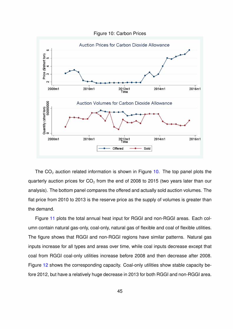
Figure 10: Carbon Prices

The CO2 auction related information is shown in Figure 10. The top panel plots the

quarterly auction prices for CO2 from the end of 2008 to 2015 (two years later than our

analysis). The bottom panel compares the offered and actually sold auction volumes. The

flat price from 2010 to 2013 is the reserve price as the supply of volumes is greater than

the demand.

Figure 11 plots the total annual heat input for RGGI and non-RGGI areas. Each col-

umn contain natural gas-only, coal-only, natural gas of flexible and coal of flexible utilities.

The figure shows that RGGI and non-RGGI regions have similar patterns. Natural gas

inputs increase for all types and areas over time, while coal inputs decrease except that

coal from RGGI coal-only utilities increase before 2008 and then decrease after 2008.

Figure 12 shows the corresponding capacity. Coal-only utilities show stable capacity be-

fore 2012, but have a relatively huge decrease in 2013 for both RGGI and non-RGGI area.

45

Figure 11: Total Annual Heat

(a) RGGI (b) Non-RGGI

Coal capacity from flexible utilities decreases significantly after 2012. Natural gas capac-

ity show a increase over years for both RGGI and non-RGGI areas. We furthermore show

the pattern of utilization rate in Figure 13. We present the average monthly utilization rate

over individual utilities. The coal utilization rate is much higher than the natural gas utiliza-

tion rate for all areas. For the non-RGGI areas, the utilization rate of natural gas has an

increasing pattern and coal has a decreasing pattern. The RGGI area has more noise as

46

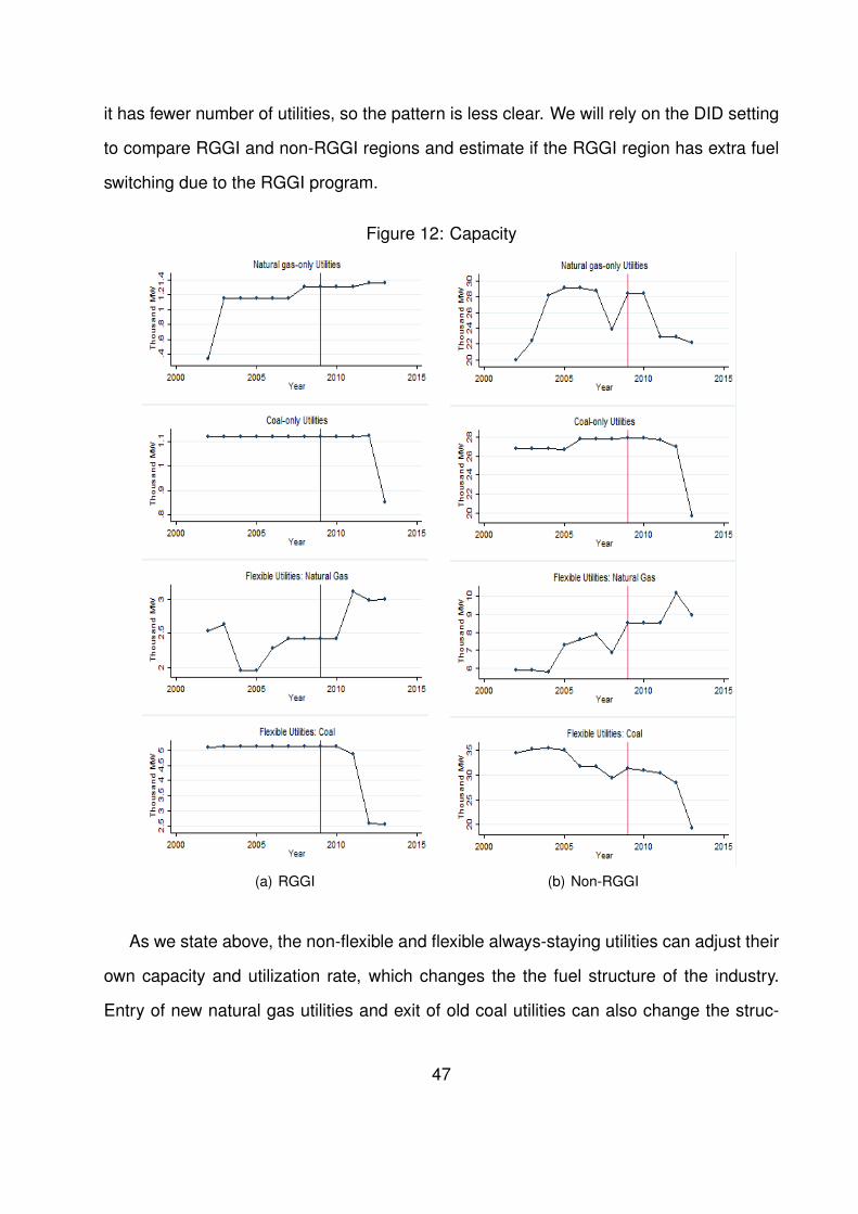
it has fewer number of utilities, so the pattern is less clear. We will rely on the DID setting

to compare RGGI and non-RGGI regions and estimate if the RGGI region has extra fuel

switching due to the RGGI program.

Figure 12: Capacity

(a) RGGI (b) Non-RGGI

As we state above, the non-flexible and flexible always-staying utilities can adjust their

own capacity and utilization rate, which changes the the fuel structure of the industry.

Entry of new natural gas utilities and exit of old coal utilities can also change the struc-

47

Figure 13: Average Utilization Rate

(a) RGGI (b) Non-RGGI

ture. For each category, adjusting utilization rate is regarded as a short-term change,

while capacity adjustment by investing in natural gas plants and divesting in coal plants

is a long-term change. In the following, we divide electricity utilities into three exclusive

categories and evaluate their fuel switching behavior separately.

48

Estimation Results: the Baseline Model

Non-flexible Always-staying Utilities

We first examine the factors that can influence the long-term fuel-switching behavior

of non-flexible always utilities. As seen from our data, natural gas power plants are newly

built and coal plants are retired. According to American Electric Power (AEP), “Simple

cycle natural gas plants are typically constructed in 18 to 30 months and combined cycle

natural gas plants are constructed in about 36 months. These lead times are significantly

less than the average for solid fuel plants (i.e. coal plants), about 72 months.”20 As natural

gas power plants require multiple years to construct, the capacity adjustment cannot occur

instantaneously. Therefore, we estimate lag models by forwarding capacity two years or

three years. Two years might be the minimum year that the capacity can respond to the

emission market. Coal plants require even longer time to construct. Retiring a coal plant

also takes a very long time as it has to be planned ahead for electricity reliability concerns

and approved by regulatory commissions. Our data time frame is not long enough, so

we assume that the coal capacity is not able to be adjusted due to the RGGI program for

simplicity.

Table 5 reports the results for the natural gas capacity adjustment model using yearly

data. The dependent variable for the first two columns is two-year lead capacity. In

Column (1), many variables are insignificant, but the coefficient for the treatment effect

After ∗ RGGI is positive and significant at 1% level. Column (2) and Column (1) are

identical except that it replaces the DID variable After ∗ RGGI with the weighted yearly

CO2 allowance price from transactions recorded by RGGI. For observations of utilities

located in non-RGGI area and year before 2009, we set the CO2 allowance price to be

0. Compared with Column (1), all other variables are quite similar and the coefficient of

CO2 price also positive and significant. The third and fourth columns report the same20See https://www.aep.com/about/IssuesAndPositions/Generation/Technologies/NaturalGas.aspx.

49

two models but with three-year lead capacity as the dependent variable. Column (3) also

shows that the RGGI program can increase the natural gas capacity for the natural gas-

only always-staying utilities three years later. The CO2 price in Column (4), again, shows

a positive and significant effect. Therefore, the natural gas-only always-staying utilities

respond to the program by increasing their capacity more than non-RGGI corresponding

utilities. We use the three-year lag model as the baseline result. Note that for all the

models, we add time-invariant fixed effect to control for unobserved heterogeneity.

Table 5: Natural Gas-Only Utilities: Total CapacityVariable Two-year lead Zitn Three-year lead Zitn

(1) (2) (3) (4)Natural gas price 0.087 0.086 0.042 0.041

(0.061) (0.061) (0.047) (0.047)Electricity price -1.487 -1.472 -0.831 -0.799

(1.294) (1.300) (0.865) (0.869)After 2.478 2.672 -3.610 -3.160

(21.191) (21.221) (15.124) (15.098)After*RGGI 43.137∗∗∗ 38.876∗∗∗

(15.086) (13.876)CO2 price 15.780∗∗ 14.659∗∗

(6.977) (5.756)Trend 0.284 0.381 0.746 0.746

(4.363) (4.361) (3.005) (2.998)CHP 20.710∗∗∗ 14.728∗∗ 16.755∗∗ 13.256∗∗

(7.992) (7.403) (6.985) (6.051)Age -1.219∗ -1.170∗ -0.931 -0.909

(0.700) (0.694) (0.631) (0.627)Ownership-Single -17.793∗∗ -17.204∗∗ -12.619∗ -12.296∗

(7.865) (7.769) (7.354) (7.276)Ownership-Other -12.670 -11.913 -11.768 -11.405

(9.369) (9.270) (8.005) (7.889)PJM annual load a -0.246 -0.258 -0.294 -0.304

(0.492) (0.492) (0.444) (0.444)Constant 1292.754∗∗∗ 1292.565∗∗∗ 1286.386∗∗∗ 1285.513∗∗∗

(60.926) (60.879) (46.375) (46.233)Utility fixed effects Yes Yes Yes YesR2 0.9853 0.9853 0.9873 0.9873Observations 421 421 379 379a Coefficients are multiplied by 107.

Robust standard errors in parentheses. ***: p < 1%, **: p < 5%, *: p < 10%.

In the short-term, utilities can adjust their heat inputs per capacity (utilization rate).

Table 6 reports the results for both natural gas-only and coal-only utilities using monthly

data. For natural gas-only utilities, the fuel price variable is natural gas price, while for

coal-only utilities, it is coal price. Again, Column (2) and (4) are identical to Column (1)

50

and (3), respectively, except replacing dummy variables After ∗RGGI with CO2 price.

For natural gas-only models, the coefficient for fuel price is negative and significant

as expected, suggesting that a higher fuel price decreases inputs. A higher electricity

price also increases heat input. Larger utilities (those with higher capacity) have a higher

utilization rate than smaller utilities. From year to year, the utilization rate has an increas-

ing trend. We also include monthly dummies and find a significant seasonal pattern: the

utilization rate is higher from May to September and December when temperature is high

or low.

We are particularly interested in the variables that are policy relevant. The variable

After captures any change before and after 2009 for all areas. Column (1) shows that

there is a statistically insignificant decrease from pre-2009 to post-2009 controlling other

factors. The coefficients of After ∗RGGI and CO2 price are the DID estimates of RGGI’s

impact on regulated utilities located in Delaware and Maryland. They are negative and

statistically significant for both models, suggesting that the RGGI program does decrease

the natural gas-only utilities’ utilization rate, surprisingly. There are two possible expla-

nations. One is that there is an emission leakage problem that RGGI utilities shift the

production to non-RGGI utilities. The other is that more non-fossil fuel replaces the fossil

fuel in the RGGI area.

For coal-only models, the signs for many coefficients are similar to the results of the

natural gas-only models. The seasonal pattern of coal use is similar that there are a much

higher utilization rate in summer and winter. The coefficients of After ∗ RGGI and CO2

prices are both significant, suggesting that coal-only utilities also decrease their utilization

rate responding to the RGGI program.

Flexible Always-staying Utilities

From the above analysis, we find that the RGGI program increases natural gas ca-

pacity investment among natural gas-only always-staying utilities, which is a relatively

longer-term adjustment. We also find short-term adjustment that both types of non-flexible

51

Table 6: Natural Gas-Only and Coal-Only Utilities: Utilization RateVariable Natural gas-only Uitn Coal-only Uitc

(1) (2) (3) (4)Natural gas price -1.014∗∗∗ -1.014∗∗∗

(0.087) (0.087)Coal price -3.412∗∗∗ -3.545∗∗∗

(0.751) (0.752)Electricity price 12.647∗∗∗ 12.651∗∗∗ 20.858∗∗∗ 20.897∗∗∗

(1.429) (1.431) (2.105) (2.105)After -16.068 -20.841 209.104∗∗ 210.613∗∗

(45.307) (45.279) (102.860) (103.004)After*RGGI -256.228∗∗∗ -578.418∗∗∗

(52.137) (135.512)CO2 price -83.997∗∗∗ -213.408∗∗∗

(20.383) (56.514)Capacity 0.260∗∗∗ 0.250∗∗∗ -5.781∗∗∗ -5.795∗∗∗

(0.059) (0.058) (0.369) (0.370)Trend 44.710∗∗∗ 44.760∗∗∗ -418.170∗∗∗ -415.124∗∗∗

(10.198) (10.197) (44.848) (44.942)CHP 185.483 218.853 1900.774∗∗∗ 1894.540∗∗∗

(163.732) (159.440) (171.776) (171.540)Age 17.851∗∗∗ 17.957∗∗∗ 274.036∗∗∗ 271.664∗∗∗

(3.676) (3.671) (38.285) (38.369)Ownership-Single 69.618 74.183 -811.729∗∗∗ -813.074∗∗∗

(56.206) (55.401) (152.208) (152.210)Ownership-Other -67.944 -63.901 -1297.950∗∗∗ -1293.342∗∗∗

(81.643) (81.060) (178.775) (178.729)PJM monthly load a -4.810∗∗∗ -4.840∗∗∗ 20.100∗∗∗ 20.200∗∗∗

(1.860) (1.860) (3.750) (3.750)Feb. -39.740 -39.101 -507.743∗∗∗ -505.268∗∗∗

(45.712) (45.771) (84.844) (84.924)Mar. -11.749 -11.492 -379.041∗∗∗ -377.299∗∗∗

(44.627) (44.678) (93.006) (93.088)Apr. -78.585 -77.968 -839.121∗∗∗ -835.974∗∗∗

(49.224) (49.259) (99.679) (99.755)May. 78.553 79.175 -1009.563∗∗∗ -1006.760∗∗∗

(60.389) (60.392) (102.342) (102.327)Jun. 220.159∗∗∗ 220.476∗∗∗ -694.894∗∗∗ -694.223∗∗∗

(46.049) (46.075) (94.085) (94.080)Jul. 560.257∗∗∗ 560.750∗∗∗ -286.148∗∗∗ -286.315∗∗∗

(71.386) (71.403) (85.263) (85.247)Aug. 529.754∗∗∗ 530.028∗∗∗ -272.006∗∗∗ -272.086∗∗∗

(62.006) (62.020) (90.735) (90.806)Sept. 162.528∗∗∗ 161.738∗∗∗ -747.984∗∗∗ -747.940∗∗∗

(43.380) (43.411) (94.161) (94.231)Oct. 8.283 7.680 -838.813∗∗∗ -838.116∗∗∗

(45.409) (45.451) (99.598) (99.660)Nov. -18.073 -16.863 -512.871∗∗∗ -508.321∗∗∗

(45.809) (45.847) (101.640) (101.708)Dec. 120.940∗∗∗ 120.544∗∗∗ -121.495 -121.976

(44.781) (44.824) (103.355) (103.447)Constant 539.705∗∗∗ 549.781∗∗∗ 2018.082∗∗∗ 2054.572∗∗∗

(195.720) (195.307) (600.673) (602.289)Utility fixed effects Yes Yes Yes YesR2 0.6036 0.6034 0.6605 0.6604Observations 6240 6240 5364 5364a Coefficients are multiplied by 106.

Robust standard errors in parentheses. ***: p < 1%, **: p < 5%, *: p < 10%.

52

utilities decrease their utilization rate. In this subsection, we investigate whether there is

evidence of short-term or long-term fuel switching for flexible always-staying utilities. We

first examine the total capacity and the percentage of natural gas capacity.

Table 7 reports the regression results using yearly data. We also estimate two-year

and three-year lagged models. Columns (1) to (4) are for the total capacity and Column

(5) to (8) are for the percentage of natural gas capacity. For the capacity percentage of

natural gas, we take logit transformation of the dependent variable. In the table, again,

Columns with even numbers replace the DID estimator After∗RGGI with weighted yearly

CO2 price. As shown in the table, the coefficients for After ∗RGGI and CO2 price are all

insignificant, suggesting that the RGGI program does not induce flexible always-staying

utilities to invest more on natural gas plants than before and other areas.

Although we find no significant change in total capacity and natural gas capacity per-

centage caused by RGGI, with the existence of the program, regulated utilities may use

natural gas plants more often even with the same natural gas capacity. We hence exam-

ine the factors that influence the utilization of capacity. The regression results are shown

in Table 8 using monthly data. The dependent variable is Uitn for Column (1) and (2), Uitc

for Column (3) and (4). The results show that a lower natural gas price leads to more

natural gas heat input per capacity. Coal heat input is not sensitive either coal or natural

gas prices. Utilities with higher total capacity have a lower utilization rate in coal than

those with lower total capacity. Higher monthly total demand in the PJM market leads

to an insignificant change in usage of natural gas but increase in coal use. Again, there

is a clear seasonal pattern. From June to September, natural gas plants are used more

often than other months during a year. Coal plants are used more often in both winter and

summer time. The coefficients for the treatment effects in four models are all significant,

indicating that the RGGI program leads to a lower utilization rate of natural gas and coal,

which is consistent to the response from natural gas-only and coal-only utilities. More

specifically, one unit increase in the CO2 allowance price causes the natural gas utiliza-

53

Table 7: Flexible Utilities: Total Capacity and Natural Gas Capacity PercentageVariable Zitn + Zitc logit(Zitn%)

Two-year lead Three-year lead Two-year lead Three-year lead(1) (2) (3) (4) (5) (6) (7) (8)

Natural gas price a -8.340 -8.530 7.780 -7.364 -0.002 -0.000 -0.003 -0.004(6.010) (6.080) (6.100) (6.132) (0.041) (0.041) (0.036) (0.036)

Coal price 2.567 2.014 5.507∗ 5.295∗ 0.004 0.006 0.003 0.004(2.749) (2.784) (2.782) (2.744) (0.011) (0.011) (0.009) (0.010)

Electricity price 17.241 18.089 4.542 3.438 -0.040 -0.045 0.057 0.061(15.239) (15.464) (13.536) (13.649) (0.067) (0.067) (0.065) (0.065)

After 347.934 324.417 -372.760 -393.224 -1.069 -0.954 1.820 1.907(379.153) (383.439) (342.877) (342.424) (1.766) (1.772) (1.564) (1.567)

After*RGGI -362.780 -459.759 0.673 1.821(298.353) (376.320) (1.280) (1.558)

CO2 price -94.387 -166.902 0.070 0.653(117.520) (152.865) (0.502) (0.635)

Capacity b 0.007 0.008 -0.461 -0.465(0.585) (0.584) (0.577) (0.577)

t -60.784 -55.535 -30.941 -27.545 0.739 0.716 0.255 0.241(101.830) (102.573) (83.710) (83.851) (0.525) (0.525) (0.440) (0.442)

CHP 223.594 188.782 234.752 222.422 1.622∗ 1.739∗ 1.820∗ 1.871∗

(161.188) (150.647) (179.168) (175.633) (0.971) (0.981) (0.981) (0.970)Age -61.818∗∗ -59.855∗∗ -49.584∗∗ -49.010∗∗ -0.235 -0.241 -0.182 -0.185

(28.145) (27.820) (22.839) (22.608) (0.147) (0.147) (0.118) (0.118)Ownership-Single -478.658 -465.856 290.180 294.601 -2.942∗ -2.987∗ -2.985∗ -3.007∗

(626.057) (626.548) (322.451) (322.564) (1.695) (1.703) (1.598) (1.594)Ownership-Other -827.349 -801.592 69.451 77.312 -3.130 -3.213 -3.682∗ -3.720∗

(725.976) (723.795) (300.860) (296.499) (2.143) (2.156) (1.931) (1.935)PJM annual load c 186.000 169.000 145.000 173.000 1.300 1.450 -0.092 -0.197

(866.000) (875.000) (811.000) (817.000) (4.340) (4.340) (4.010) (4.000)Constant 7829.006∗∗∗ 7860.583∗∗∗ 6870.464∗∗∗ 6913.343∗∗∗ 11.094 10.943 7.390 7.250

(2022.899) (2024.064) (1198.228) (1195.583) (11.697) (11.685) (9.837) (9.880)Utility fixed effects Yes Yes Yes Yes Yes Yes Yes YesR2 0.9370 0.9366 0.9443 0.9441 0.7360 0.7355 0.7786 0.7779Observations 163 163 147 147 163 163 147 147a Coefficients are multiplied by 10.b Coefficients are multiplied by 103.c Coefficients are multiplied by 109.

Robust standard errors in parentheses. ***: p < 1%, **: p < 5%, *: p < 10%.

tion rate to decrease by about 120 MMtbu/thousand MW, and causes the coal utilization

rate to decrease by 423 MMtbu/thousand MW. Overall, we find that flexible utilities and

non-flexible utilities have similar emission reduction strategies. They all tend to use the

short-term method by reducing heat input. Only the natural gas-only utilities have been

found also adjusting their capacity, which is a long-term method.

Entry and Exit of Utilities

The last fuel switching behavior between natural gas and fuel we intend to examine

is through entry and exit of fossil fuel utilities. Coal utilities usually exit and natural gas

utilities enter. In our data, there are altogether 124 utilities, 13 of them are located in

54

Table 8: Flexible Utilities: Natural Gas and Coal Utilization RateVariable Uitn Uitc

(1) (2) (3) (4)Natural gas price -0.783∗∗∗ -0.770∗∗∗ -0.148 -0.135

(0.145) (0.144) (0.197) (0.200)Coal price 0.184 -0.041 0.250 -0.887

(0.449) (0.423) (0.874) (0.870)Electricity price 14.628∗∗∗ 14.616∗∗∗ 22.983∗∗∗ 23.545∗∗∗

(4.274) (4.294) (3.367) (3.417)After 569.424∗∗∗ 568.477∗∗∗ 649.493∗∗∗ 610.896∗∗∗

(211.988) (209.851) (147.779) (149.534)After*RGGI -323.897∗∗∗ -1291.242∗∗∗

(94.290) (136.905)CO2 price -119.942∗∗∗ -422.861∗∗∗

(31.510) (60.233)Capacity -0.056 -0.055 -0.339∗∗∗ -0.335∗∗∗

(0.041) (0.041) (0.050) (0.051)t 37.330 40.325∗ -348.802∗∗∗ -333.831∗∗∗

(25.036) (24.401) (36.559) (36.490)CHP 80.346 71.126 -902.782∗∗∗ -971.068∗∗∗

(71.658) (70.802) (135.293) (140.889)Age -76.025∗∗∗ -76.054∗∗∗ 27.677 26.887

(6.777) (6.809) (18.445) (18.359)Ownership-Single 256.398∗∗∗ 257.702∗∗∗ 239.336∗ 249.856∗

(85.801) (86.179) (131.959) (132.637)Ownership-Other 166.013∗ 172.303∗ 480.604∗∗∗ 531.963∗∗∗

(92.374) (91.364) (171.700) (172.318)PJM monthly load a -0.001 -0.001 0.017∗∗∗ 0.017∗∗∗

(0.003) (0.003) (0.005) (0.005)Feb. -15.172 -10.838 -297.028∗∗ -280.721∗∗

(51.745) (51.811) (135.168) (136.856)Mar. 112.258 115.546 -342.326∗∗ -328.719∗∗

(96.748) (97.070) (143.835) (145.242)Apr. 63.978 69.473 -859.920∗∗∗ -837.603∗∗∗

(60.202) (60.533) (146.024) (148.394)May. 153.410∗∗ 159.125∗∗ -896.442∗∗∗ -872.332∗∗∗

(70.883) (71.344) (137.427) (138.854)Jun. 272.021∗∗∗ 275.713∗∗∗ -444.492∗∗∗ -432.488∗∗∗

(93.874) (93.927) (131.756) (133.480)Jul. 590.324∗∗∗ 595.351∗∗∗ -217.770 -205.818

(188.126) (188.544) (138.535) (140.661)Aug. 484.206∗∗∗ 488.432∗∗∗ -295.183∗∗ -284.113∗∗

(144.380) (144.598) (135.747) (137.424)Sept. 214.095∗∗∗ 214.136∗∗∗ -603.077∗∗∗ -600.031∗∗∗

(64.974) (64.974) (128.189) (129.553)Oct. 126.073∗∗ 126.516∗∗ -853.334∗∗∗ -847.067∗∗∗

(58.641) (58.657) (137.790) (138.561)Nov. 109.359∗ 117.663∗ -708.855∗∗∗ -673.701∗∗∗

(61.051) (61.981) (135.867) (137.275)Dec. 72.715 72.627 -418.524∗∗∗ -414.514∗∗∗

(49.773) (49.756) (144.282) (145.375)Constant 2482.944∗∗∗ 2526.304∗∗∗ 2932.554∗∗∗ 3166.971∗∗∗

(279.526) (284.185) (1036.922) (1031.896)Utility fixed effects Yes Yes Yes YesR2 0.1801 0.1801 0.6172 0.6134Observations 2376 2376 2376 2376a Coefficients are multiplied by 103.

Robust standard errors in parentheses. ***: p < 1%, **: p < 5%, *: p < 10%.

55

Delaware and Maryland. During the sample period the exit at utility level is minimal:

Only one utility located in Pennsylvania exited the market before 2009.21 Among the 124

utilities, 9 entered after 2009, and only one of them is within the RGGI region. From 2009

to 2013, the entering capacity counts for 4.43% of the total capacity in the whole PJM

area. Therefore, the RGGI policy impact on utilities’ entry & exit decisions is minimal.

Robustness Check and Causality

The previous baseline models test whether the RGGI program is effective in inducing fuel

switching and how utilities respond. In this section we apply multiple tests to check the

robustness of previous results.

11.1 Specification Check

We first repeat all the previous analyses with logged dependent variables. Since the

utilization rate could be equal to zero, we add 1 to the rate and then take the logarithm

format. All the regression results are reported in Appendix A. We find that with logged

format of dependent variables, all the results are robust to the specification except that

the treatment effect becomes weakly significant for the natural gas utilization rate in the

flexible utilities. We will discuss this more later.

11.2 Falsification Tests

Next we use falsification tests to check if our model specification produces spurious re-

sults. In the tests, we include only utilities in unregulated states (the control group in

previous analysis) in the PJM area, and then create "fake" treatment groups by randomly

assign treatment to half of the sample. Under this scenario, the treatment effects are21Moreover, it exited after year 2004, which was well before the proposition of RGGI.

56

Table 9: Falsification Tests: Random TreatmentNatural gas-only Coal-only Flexible-natural gas Flexible-coal

Variable Three-year lead Zitn Uitn Uitc Uitn Uitc

(1) (2) (3) (4) (5)Natural gas price 0.049 -1.046∗∗∗ -0.719∗∗ -0.533∗∗

(0.062) (0.094) (0.298) (0.242)Coal price -4.193∗∗∗ 3.089∗ -2.914∗

(0.865) (1.859) (1.509)Electricity price -0.850 12.917∗∗∗ 20.048∗∗∗ 16.341∗∗∗ 20.171∗∗∗

(1.149) (1.558) (2.211) (5.151) (4.180)After 1.152 -60.184 324.005∗∗∗ 548.609∗∗ 133.950

(21.275) (50.676) (113.693) (216.882) (175.981)After*RGGI 9.613 -2.703 -38.471 48.212 74.844

(10.558) (34.379) (70.186) (118.135) (95.856)Capacity 0.339∗∗∗ -5.634∗∗∗ -0.103∗∗ -0.410∗∗∗

(0.060) (0.387) (0.052) (0.042)t -0.781 56.199∗∗∗ -438.178∗∗∗ 1.017 -238.176∗∗∗

(4.136) (11.044) (48.845) (43.881) (35.606)CHP 26.656 588.679∗∗ 1878.771∗∗∗ -377.040 -442.126∗∗

(16.346) (272.946) (171.852) (247.242) (200.615)Age -1.195 16.139∗∗∗ 285.549∗∗∗ -73.213∗∗∗ 29.788∗∗∗

(0.809) (3.759) (41.319) (13.186) (10.699)Ownership-Single -15.020 104.406∗ -818.577∗∗∗ 199.523 227.245

(10.369) (60.552) (152.462) (185.081) (150.177)Ownership-Other -15.696 -32.750 -1267.488∗∗∗ 53.565 385.614∗

(11.907) (84.825) (179.270) (262.088) (212.662)PJM load a -6.590 -614.000∗∗∗ 2180.000∗∗∗ -329.000 1370.000∗∗

(6.640) (204.000) (401.000) (676.000) (549.000)Feb. -49.693 -513.533∗∗∗ -20.393 -295.746∗∗

(49.641) (88.748) (185.151) (150.234)Mar. -18.597 -368.761∗∗∗ 130.409 -359.042∗∗

(48.611) (96.440) (185.548) (150.556)Apr. -107.690∗∗ -830.267∗∗∗ 49.621 -899.192∗∗∗

(53.020) (105.398) (193.923) (157.351)May. 66.038 -991.679∗∗∗ 147.974 -826.576∗∗∗

(65.789) (107.905) (187.278) (151.960)Jun. 213.757∗∗∗ -712.164∗∗∗ 263.373 -422.208∗∗∗

(49.883) (99.256) (183.561) (148.943)Jul. 569.332∗∗∗ -304.771∗∗∗ 601.445∗∗∗ -198.154

(77.573) (88.275) (195.993) (159.031)Aug. 541.684∗∗∗ -306.789∗∗∗ 449.173∗∗ -257.456∗

(67.495) (95.939) (192.029) (155.815)Sept. 153.920∗∗∗ -773.711∗∗∗ 154.954 -626.552∗∗∗

(47.154) (99.418) (184.959) (150.078)Oct. 3.519 -856.026∗∗∗ 94.245 -727.887∗∗∗

(49.280) (104.604) (186.441) (151.280)Nov. -20.250 -518.579∗∗∗ 113.988 -686.264∗∗∗

(49.898) (107.515) (186.942) (151.687)Dec. 129.565∗∗∗ -102.618 53.893 -337.826∗∗

(48.592) (109.412) (183.398) (148.811)Constant 1313.903∗∗∗ 533.555∗∗∗ -1082.363 2009.734∗∗ 4930.363∗∗∗

(49.269) (204.117) (1071.766) (830.980) (674.267)Utility fixed effects Yes Yes Yes Yes YesR2 0.9841 0.6028 0.6503 0.1616 0.6211Observations 267 5688 4944 1668 1668a Coefficients are multiplied by 108.

Robust standard errors in parentheses. ***: p < 1%, **: p < 5%, *: p < 10%.

supposed to be zero. If the treatment effects for the "fake" treatment groups are different

from 0, then our previous results are likely to be biased. Table 9 reports the results of

falsification tests for the previous regression models with significant results. As shown in

57

the table, the coefficients of After ∗ RGGI are all not statistically significant. The results

show that since no significant impact of RGGI is found, it is a good sign that our significant

results are not spurious.

11.3 Event Study-Style Model

In the previous DID framework, we have a single coefficient for treatment effect. It does

not allow for heterogeneous effects varying before and after the policy year. In the follow-

ing, we re-estimate event study-style models allowing for heterogeneous effects, the new

model can be written as:

Yitx =β0 + β1Pitx + β2Pet + β3trendyear + β4Demandt + β5Sit

+T∑

year=1dyearDyear +

T∑year=1

γyearDyear ∗RGGIi + αi + εit for x = c, n(13)

The difference between this framework and the previous one is that instead of using

Afteryear, we use dummy variables for each year (Dyear), and instead of using Afteryear ∗

RGGIi, we use Dyear ∗ RGGIi. Therefore, there is a different coefficient each year for

the effect. After obtaining the yearly effect, we test whether there is a break in the yearly

effect due to the policy using the following model:

γyear = r0 + r1Afteryear + r2trendyear + r3Afteryear ∗ trendyear + ζyear (14)

Figure 14 presents the event study graphs of the yearly effect, γyear, from estimating

Equation 13. Panel (a) to (d) show yearly effects on the utilization rate of natural gas-only

utilities, coal-only utilities, flexible utilities-natural gas and flexible utilities-coal respectively.

The year of policy year, 2009, is denoted by zero and marked with a vertical line in all

panels. The Zero effect is noted by a horizontal line.

These figures visually reveal the possible pattern of the policy impact. Except the

58

Figure 14:

(a) (b)

(c) (d)

flexible utilities-natural gas, other utilities have a close to zero impact before policy year,

suggesting that the impact on utilization rate in the RGGI area are similar to non-RGGI

utilities. For the flexible utilities-natural gas, the impact does not start with zero, but with

some negative value meaning that such RGGI utilities have a lower value before 2009

compared to non-RGGI utilities.

Among all utilities, flexible utilities-coal are more likely to have a clear break in the

policy year just by visually examining the graph. More formal tests are reported in Table

10. Column (3) is the full model for Equation 14, while Column (1) only contains a dummy

for After and Column (2) allows for a dummy for After and a time trend. The full model

is more flexible and additionally allows for different trend after 2009. We list the results,

again, by the order of natural gas-only utilities, coal-only utilities, flexible utilities-natural

59

gas and flexible utilities-coal. The results show that if allowing for the maximum flexibility

(Column (3)), natural gas utilities for both flexible and non-flexible utilities do not have a

break in the policy year because both coefficients for After and After ∗ t are not signifi-

cant, suggesting that the RGGI policy impact is not significant. However, the tests for coal

utilities show that there is a clear significant policy impact. Concerning that there are only

11 observations, the evidence is strong that coal utilities respond to the RGGI policy by

reducing their utilization rate.

Table 10: Break Tests For Yearly Effects

Generating Utilities (1) (2) (3)Natural Gas Only Utilities

After -280.336∗∗ -53.471 -45.579(102.679) (118.890) (113.697)

Trend -42.539∗ -25.236(22.742) (22.622)

After*Trend -53.154(66.487)

Constant -28.935 -175.633∗ -115.961(46.423) (79.453) (86.673)

Coal Only Utilities

After -409.771 -1933.216∗∗∗ -1942.225∗∗∗

(378.913) (286.958) (330.957)Trend 273.466∗∗∗ 245.821∗∗∗

(67.377) (47.247)After*Trend 80.522

(173.017)Constant 2.446 972.268∗∗∗ 874.229∗∗∗

(205.322) (228.994) (140.207)Flexible Utilities- Natural Gas

After -250.348 -354.653 -383.146(179.598) (301.934) (338.584)

Trend 18.601 -37.170(50.188) (35.093)

After*Trend 162.720(114.475)

Constant -498.233∗∗∗ -432.935∗ -628.715∗∗∗

(70.612) (216.270) (129.856)Flexible Utilities- Coal

After -1054.226∗∗ -462.933 -485.917(419.054) (891.236) (306.703)

Trend -110.300 132.006∗∗

(148.970) (46.446)After*Trend -688.427∗∗∗

(88.998)Constant 397.250∗∗∗ 10.394 860.236∗∗∗

(121.438) (589.792) (180.232)Observations 11 11 11

60

11.4 Pre-policy Effects

Although the RGGI program is effective on January 1, 2009, the history of the initiative

goes back to 2003 when nine states start the discussion. Early in December of 2005, a

Memorandum of Understanding (MOU) is signed to implement the Regional Greenhouse

Gas Initiative. Delaware signed it in December, 2005, joined by Maryland in 2007. There-

fore, utilities in Delaware and Maryland were aware of their obligation before 2009. So it

is possible for them to respond to the program before 2009. In order to understand the

pre-policy effects, we restrict the year of observations to 2002-2008 only, and set 2006 to

be the first year of agreement (the middle year for Delaware and Maryland) and rerun the

basic analyses for policy impact on utilization rate.

Table 11 reports the results. Column (1) to (4) are models of utilization rate for natural

gas-only utilities, coal-only utilities, flexible utilities-natural gas and flexible utilities-coal

respectively. The results show that the policy announcement does not affect the natural

gas-only utilities while affect others. Specifically, the announcement decreases the utiliza-

tion rate for flexible utilities-natural gas by 203.73 MMtbu/thousand MW, which is lower

than the policy implementation effect (323.90 MMtbu/thousand MW) but with the same

direction. Opposite to the policy impact of implementation, the announcement increases

the utilization rate for coal in both flexible and non-flexible utilities. This suggests that coal

utilities are aware that they need to pay for CO2 emission after 2009 and will reduce coal

use after 2009, so they in fact increase coal use before 2009 and after announcement.

Such evidence of pre-policy effect raises an issue that the impact of policy implemen-

tation identified in the baseline model might be over-estimated for the coal utilities as they

deliberately increased the coal use right before 2009. In the other hand, the estimation

for flexible utilities-natural gas might be under-stated. Unfortunately, we are not able to

isolate the bias, but just document the caveat here.

61

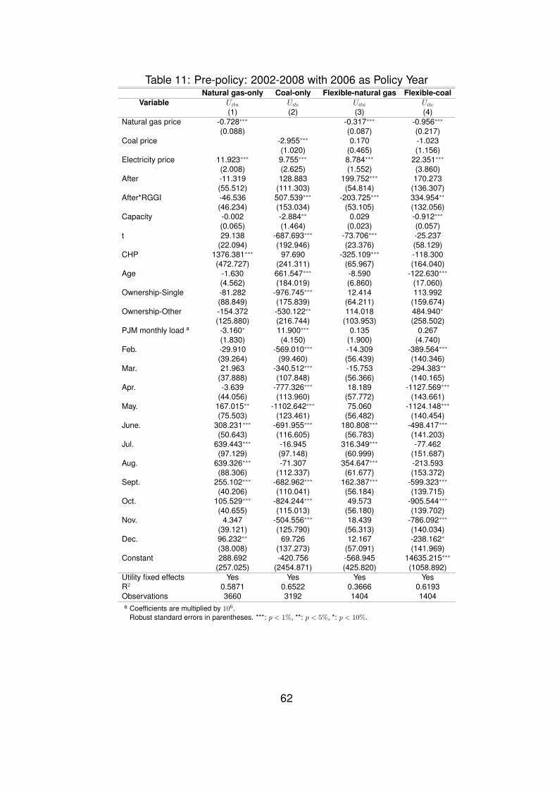
Table 11: Pre-policy: 2002-2008 with 2006 as Policy YearNatural gas-only Coal-only Flexible-natural gas Flexible-coal

Variable Uitn Uitc Uitn Uitc

(1) (2) (3) (4)Natural gas price -0.728∗∗∗ -0.317∗∗∗ -0.956∗∗∗

(0.088) (0.087) (0.217)Coal price -2.955∗∗∗ 0.170 -1.023

(1.020) (0.465) (1.156)Electricity price 11.923∗∗∗ 9.755∗∗∗ 8.784∗∗∗ 22.351∗∗∗

(2.008) (2.625) (1.552) (3.860)After -11.319 128.883 199.752∗∗∗ 170.273

(55.512) (111.303) (54.814) (136.307)After*RGGI -46.536 507.539∗∗∗ -203.725∗∗∗ 334.954∗∗

(46.234) (153.034) (53.105) (132.056)Capacity -0.002 -2.884∗∗ 0.029 -0.912∗∗∗

(0.065) (1.464) (0.023) (0.057)t 29.138 -687.693∗∗∗ -73.706∗∗∗ -25.237

(22.094) (192.946) (23.376) (58.129)CHP 1376.381∗∗∗ 97.690 -325.109∗∗∗ -118.300

(472.727) (241.311) (65.967) (164.040)Age -1.630 661.547∗∗∗ -8.590 -122.630∗∗∗

(4.562) (184.019) (6.860) (17.060)Ownership-Single -81.282 -976.745∗∗∗ 12.414 113.992

(88.849) (175.839) (64.211) (159.674)Ownership-Other -154.372 -530.122∗∗ 114.018 484.940∗

(125.880) (216.744) (103.953) (258.502)PJM monthly load a -3.160∗ 11.900∗∗∗ 0.135 0.267

(1.830) (4.150) (1.900) (4.740)Feb. -29.910 -569.010∗∗∗ -14.309 -389.564∗∗∗

(39.264) (99.460) (56.439) (140.346)Mar. 21.963 -340.512∗∗∗ -15.753 -294.383∗∗

(37.888) (107.848) (56.366) (140.165)Apr. -3.639 -777.326∗∗∗ 18.189 -1127.569∗∗∗

(44.056) (113.960) (57.772) (143.661)May. 167.015∗∗ -1102.642∗∗∗ 75.060 -1124.148∗∗∗

(75.503) (123.461) (56.482) (140.454)June. 308.231∗∗∗ -691.955∗∗∗ 180.808∗∗∗ -498.417∗∗∗

(50.643) (116.605) (56.783) (141.203)Jul. 639.443∗∗∗ -16.945 316.349∗∗∗ -77.462

(97.129) (97.148) (60.999) (151.687)Aug. 639.326∗∗∗ -71.307 354.647∗∗∗ -213.593

(88.306) (112.337) (61.677) (153.372)Sept. 255.102∗∗∗ -682.962∗∗∗ 162.387∗∗∗ -599.323∗∗∗

(40.206) (110.041) (56.184) (139.715)Oct. 105.529∗∗∗ -824.244∗∗∗ 49.573 -905.544∗∗∗

(40.655) (115.013) (56.180) (139.702)Nov. 4.347 -504.556∗∗∗ 18.439 -786.092∗∗∗

(39.121) (125.790) (56.313) (140.034)Dec. 96.232∗∗ 69.726 12.167 -238.162∗

(38.008) (137.273) (57.091) (141.969)Constant 288.692 -420.756 -568.945 14635.215∗∗∗

(257.025) (2454.871) (425.820) (1058.892)Utility fixed effects Yes Yes Yes YesR2 0.5871 0.6522 0.3666 0.6193Observations 3660 3192 1404 1404a Coefficients are multiplied by 106.

Robust standard errors in parentheses. ***: p < 1%, **: p < 5%, *: p < 10%.

62

Emission Reduction

12.1 Emission Reduction and Fuel Switching

In the previous sections, we have examined how the RGGI could potentially induce the

fuel switching behavior and conducted multiple robustness tests. However, only with re-

gression results, we are not clear about the magnitude of emission reduction. In this

section, we will calculate counterfactuals to quantify the emission reduction.

The counterfactual change can be calculated according to the regression results in

Column (3) of Table 5, and Columns (1) and (3) of Table 6 and 8. In fact for the natural

gas-only utilities, the RGGI program effectively increases the capacity by 38.88 MW on

average three years later. The utilization rate decreases by 256.23 MMbtu/thousand MW

for natural-gas only utilities, and 578.42 MMbtu/thousand MW for coal-only utilities. We

can calculate the counterfactuals with and without policy according to Equation 8. For

the flexible utilities, the program induces an average utility to decrease the natural gas

utilization rate by 323.90 MMbtu/thousand MW, and decrease the coal utilization rate by

1291.24 MMbtu/thousand MW. Given the total fossil capacity (Zitn + Zitc) for a regulated

flexible utility, we can calculate its change of fuel use using Equation 10. In the coun-

terfactual scenario when there is no RGGI program, the treatment coefficient is set to

zero.

The changes due to the RGGI program can be read from Table 12. It reports the

annual heat input with and without the RGGI program in Delaware and Maryland. For the

natural gas-only utilities, we consider the capacity adjustment after 2012 (three years after

2009) and consider the adjustment of utilization rate after 2009. The total natural gas heat

input is 48.15 million MMBtu with policy for the period of 2009 to 2013, while if without

policy the input increases by 17.94 million MMBtu. The capacity increase accounts for

2.41 million MMBtu increase in natural gas heat input, while the utilization rate adjustment

accounts for 20.35 million MMBtu decrease in natural gas heat input. So overall the

63

the RGGI program leads to 17.94 million MMBtu reduction in natural gas input, which is

37.26% of their total heat input. In contrast, the natural gas heat input of flexible always-

staying utilities decreases by 49.30 million MMBtu over the period 2009 to 2013, which

is 27.14% of their own total input. The coal heat input of coal-only utilities decreases by

37.05 million MMBtu from 2009 to 2013 in total, or about 20.34% of their total coal input,

while the coal heat input of flexible utilities decreases by 285.40 million MMBtu which is

38.69% of their total coal input.

Table 12: Emission Reduction in RGGI Area : 2009-2013

Generating Utilities 2009 2010 2011 2012 2013 TotalNatural Gas Only UtilitiesWith policy 7.18 10.74 8.41 10.22 11.60 48.15Without policy change-capacity -1.06 -1.35 -2.41Without policy change-utilization +4.01 +4.01 +4.01 +4.16 +4.16 +20.35Without policy change-overall +4.01 +4.01 +4.01 +3.10 +2.81 +17.94Emission Change (Thousand Short Tons) -234.59 -234.59 -234.59 -181.35 -164.39 -1049.49Coal Only UtilitiesWith policy 40.61 43.84 32.78 31.94 33.00 182.17Without policy change +7.78 +7.78 +7.78 +7.81 +5.90 +37.05Emission Change (Thousand Short Tons) -836.35 -836.35 -836.35 -839.58 -634.25 -3982.88Flexible Utilities- Natural GasWith policy 12.73 26.55 40.69 57.17 44.49 181.63Without policy change +9.39 +9.39 +12.10 +11.59 +11.66 +54.13Emission Change (Thousand Short Tons) -549.32 -549.32 -707.85 -678.02 -682.11 -3166.61Flexible Utilities- CoalWith policy 236.76 229.35 112.83 82.37 76.34 737.65Without policy change +79.06 +79.06 +75.16 +40.07 +39.79 +313.04Emission Change (Thousand Short Tons) -8498.95 -8498.95 -8079.70 -4307.53 -4277.43 -33651.80Natural gas heat input percentage 2009 2010 2011 2012 2013 AverageWith policy 6.70% 12.01% 25.22% 37.09% 33.91% 22.98%The Baseline ModelChange due to policy -1.64% -0.36% +2.80% +3.27% +2.45% +1.30%The Event Study-style ModelChange due to policy +1.42% +2.46% +7.10% +7.27% +6.89% +5.03%

Given the information of heat input change, we can directly calculate the emission

change. 22 Overall, the RGGI program leads to 7.72 million short tons of CO2 reduction

per year in Delaware and Maryland, which is about 34.36% of the average total annual

emissions in these two states from 2009 to 2013. However, as discussed in the sections

of “Specification Check” and “Event Study-style Model”, models for natural gas are not22In our data, the correlation between CO2 and heat input is 0.99.

64

as robust as coal models. To be conservative, if we only calculate the emission reduc-

tion through coal utilities only, the fuel switching under the RGGI program causes 6.93

million short tons of CO2 reduction per year, or about 35.06% of the average total annual

emissions.

Table 12 also reports the natural gas input rate change due to the program imple-

mentation. With the baseline model, the program implementation changes the rate from

21.68% to 22.98% on average between 2009 and 2013. If using the results from the event

study-style model, the implementation increases the percentage from 17.96% to 22.98%.

For both cases, natural gas heat input rate increases due to the program.

12.2 Replacement for Reduced Coal in RGGI

In Delaware and Maryland, we observe that coal heat input has decreased and natural

gas input has increased, but the decreased coal input cannot be covered by the increased

coal input. We then need to examine what replaced the gap left by coal reduction. One

potential way is to increase the non-fossil fuel input within the RGGI area. The other way

is simply to shift the production to non-RGGI areas. We use two tests to test these two

hypotheses, which are reported in Table 13. In the first column, we regress the total power

generation in each state of Delaware and Maryland excluding generation from natural

gas and coal23 on the After dummy and other monthly dummies, and find that non-

fossil fuel generation did not increase as the coefficient for After is insignificant. In the

second column, we first define the import of electricity of one state as total consumption

minus total power generation by the utilities located in the state, and then regress the

monthly import on the After dummy and other monthly dummies. We find that the import

increased significantly after 2009. This is, in fact, an evidence for the emission leakage

problem. Two tests combined show that emission reduction in Delaware and Maryland

due to the RGGI program is not achieved by replacing fossil fuel (natural gas and coal) by23The power generation from petroleum is very small.

65

non-fossil, but by leaking emissions to non-RGGI areas. It reveals an important fact that

leaking emissions to other non-RGGI areas is less costly than fuel switching.

Table 13: Replacement for Reduced Coal in RGGI

RGGI States Neighboring StatesOther Generation Import Other Generation Import

After -249.631∗∗∗ 543.888∗∗∗ 258.645∗ 3285.331∗∗∗

(33.525) (64.558) (137.058) (1112.796)Feb. -506.000∗∗∗ 290.833 -1955.250∗∗∗ 1041.500∗

(106.432) (210.635) (324.738) (593.693)Mar. -562.250∗∗∗ 81.333 -2052.250∗∗∗ -1157.333

(114.010) (181.464) (352.750) (2407.507)Apr. -354.083∗∗∗ -350.583∗ -3476.083∗∗∗ -387.333

(104.038) (188.435) (268.032) (2277.857)May. -276.917∗∗ -326.667 -2260.667∗∗∗ 314.250

(116.695) (219.579) (288.443) (543.904)Jun. -269.000∗∗∗ -215.083 -1589.167∗∗∗ -669.750

(99.373) (170.265) (293.909) (504.135)Jul. -202.333∗ -52.917 -353.667 -4182.917∗

(103.313) (165.280) (447.545) (2450.871)Aug. -198.083∗ 126.417 -609.000∗∗∗ -6583.000∗∗

(107.338) (175.692) (215.857) (3298.473)Sept. -328.417∗∗∗ 3.667 -2321.583∗∗∗ 1215.667∗

(94.616) (170.104) (289.774) (630.818)Oct. -233.083∗∗ -447.917∗∗ -2988.667∗∗∗ -6015.083

(103.044) (202.556) (263.426) (3788.471)Nov. -345.000∗∗∗ -374.833∗∗ -2497.333∗∗∗ -1479.083

(93.078) (179.049) (279.665) (2225.681)Dec. -83.417 -126.667 -253.250 -890.833

(106.167) (190.829) (299.333) (643.641)Constant 2018.763∗∗∗ 1835.297∗∗∗ 15898.231∗∗∗ -6389.471∗∗∗

(90.082) (156.320) (197.540) (625.450)R2 0.4663 0.4880 0.6636 0.1717Observations 144 144 144 144

66

Discussion and Conclusion

In this paper, we empirically test the role of fuel switching in a carbon emission market

under the context of the RGGI program. Fuel switching between natural gas and coal in-

cludes long-term capacity adjustment and short-term input adjustment. We find statistical

evidence that the RGGI program is effective in reducing emissions, but mainly through

reduction of coal and natural gas inputs. We find that the program is responsible for 7.72

million short tons of CO2 reduction under the program, which is 34.36% of the average

total annual emissions in Delaware and Maryland from 2009 to 2013. We also find that

flexible and non-flexible utilities have adopted similar reduction strategies. All utilities tend

to decrease utilization rate, except natural gas-only utilities adopt longer-term method

through increasing capacity additionally.

Our major findings are based on comparing treatment and control groups. We have

applied separate DID analyses to different utility categories: natural-gas only and coal-

only utilities and flexible utilities. The separate analyses help prevent the endogeneity

issue of the RGGI program, i.e. states who are easier to fuel switch are more likely to join

the RGGI program. For example, a state with a higher capacity rate of natural gas may

be easier to reduce CO2 emissions. As the treatment and control groups are in the same

category in terms of fuel type, we face a less severe problem.

Although our results show that utilities do respond to the not very high CO2 price in the

emission trading program, we find that the RGGI program leads to neither fuel switching

from coal to natural gas nor from fossil fuel to non-fossil fuel. Instead, emission leakage

occurred. It reveals an important fact that under the CO2 emission trading program, it is

less costly to reduce CO2 by leaking emissions to non-RGGI areas than using more non-

fossil fuel or more natural gas. In the other words, the CO2 emission trading program can

provide incentives for emission reduction. However, under the current regional program,

shifting emissions to other areas is, unfortunately, the first option. Therefore, we need to

67

be conservative about the CO2 emission reduction due to the emission trading program if

the program becomes national in the future.

There are a few caveats to our analyses that should be noted. First, our model does

not control for vertical arrangement. To hedge risk, power plants often sign long-term

contracts with electricity retailers to supply electricity. Such a fixed commitment can af-

fect industry structure (Wolak, 2000) and change producers’ behavior (Fabra and Toro,

2005). Bushnell et al. (2008a) emphasize the importance of accounting for the vertical

arrangement in the electricity price equilibrium model. In addition, power plants also tend

to sign long-term contracts with fuel suppliers (Jha, 2015). All these long-term contracts

are constraints on power firms that are not taken into account in our model. Firm fixed

effects may help alleviate the problem, however. Second, although we account for other

types of pollutants in our profit maximization problem, we do not have sufficient informa-

tion to isolate the empirical influence of regulations on other pollutants. Last but not least,

the impact of the RGGI program may take a long time to fully emerge, and the equilibrium

could change over time. Our results should be viewed as measuring the program’s impact

in the short run.

68

Chapter Three

Emission Responses to Carbon Pricing in Dynamic Electricity Markets

Yishu Zhou

University of Connecticut

Abstract

The Regional Greenhouse Gas Initiative (RGGI) regulates CO2 emissions from the power

sector in the nine northeastern states of the U.S.. The effectiveness of RGGI has long

been criticized due to the low CO2 allowance price and limited price variation. Using a

model that accounts for intertemporal constraints, this paper studies electricity generators’

production behavior and how the decisions are altered with CO2 emission regulations.

The results show that the RGGI policy has helped to decrease the total CO2 emissions

by at least 4.73% during the sample period. All other things equal, an additional $1/ton

increase in permit price reduce the total CO2 emissions by 1.85%. CO2 can be reduced

by 23.50% if carbon is priced at $15/ton. I also find slight evidence of fuel switching from

coal to natural gas.

Keywords: Carbon Emission Market, RGGI, Emission Responses

69

Introduction

To regulate air pollution in the electricity industry, market-based emission trading pro-

grams have been widely adopted around the world since the 1990s. The first national

emissions cap and trade program in the U.S. was the Acid Rain Program (ARP), estab-

lished under Title IV of the 1990 Clean Air Act (CAA) Amendments. It requires power

plants to reduce emissions of sulfur dioxide (SO2) and nitrogen oxides (NOx), the primary

precursors of acid rain. However, similar programs for greenhouse gas (GHG) emis-

sions were not established until rather recently. The European Union Emissions Trading

Scheme (EU ETS) is the first and largest GHG emissions trading scheme in the world.

In the U.S., although lacking of CO2 regulations at the national level, some regional pro-

grams have been formed, such as the RGGI and the Western Climate Initiative (WCI).

On June 2, 2014, the United States Environmental Protection Agency (EPA) proposed a

nationwide plan to cut carbon pollution from power plants in all states. The study of exist-

ing regional GHG emission trading programs can provide important information for future

regulations, at both regional and federal levels.

Using a model that accounts for intertemporal constraints, this paper studies electricity

generators’ production behavior and how the decisions are altered with CO2 emission

regulations. Unlike many other markets, the electricity market is highly complex with

several notable features. Since it is extremely costly to store electricity on a large scale,

and demand and wholesale electricity price fluctuate significantly within a day and across

seasons, firms respond by making distinct production decisions from hour to hour. As

a result, total capacity, which is the maximum electric output in an hour, is high in order

to avoid power outage during peak load times. On the other hand, many generators are

brought offline to match supply with lower demand during off-peak hours.

In this paper I study individual producers separately with hourly data. Many works

studying emissions have been done at the aggregate level. Vollebergh et al. (2009) and

70

Holtz-Eakin and Selden (1995) use country-level panel data to investigate the relation-

ship between emissions and variables such like income and per capita GDP. Auffhammer

and Carson (2008) forecast China’s CO2 emissions by using province-level data. They

conclude that emissions in China are unlikely to decrease in the near future unless sub-

stantial changes in energy policies occur. Using state-level data, Murray et al. (2014)

quantify the emissions reduction due to RGGI with a three-stage model to estimate state

demand, demand by fuel type and emission, respectively. However, aggregate data do

not incorporate the important features of electricity markets into the analysis, and thus

cannot fully explain and predict individual producers’ detailed reaction to the complex

market conditions which could vary from hour to hour.

As Mansur (2008) and Cullen (2015) point out, electricity generation cannot be smoothly

adjusted from zero to full capacity at will due to technology limitations. Ramp rate, which

is the maximum increase or decrease in output per hour, limits how fast a generator can

make adjustment. Furthermore, when a generator is shut down, a start-up cost is in-

curred to bring it back online, which is significant and cannot be ignored (Reguant, 2014).

Minimum load limits how little the production can be for a generator to remain operating

in order to avoid paying the start-up cost. These intertemporal constraints impede out-

put adjustment, and make current production depend heavily on the operating status in

the previous period. Moreover, a generator aiming a high production in the future due to

high expected price may need to start increasing production from now. Therefore, current

production level is correlated with both past and future productions.

Very few studies recognize the importance of intertemporal constraints in the electric-

ity markets. Mansur (2008) examines the welfare loss resulted from market power after

restructuring in electricity markets. He finds that ignoring intertemporal constraints leads

to overestimation of the welfare loss. Cullen (2015) structurally estimates production costs

(including start-up cost), and then compute competitive equilibria under different environ-

mental policies. Instead of causing immediate emission reduction, the results show that

71

carbon pricing influences firms’ profits and affects their long-run investment decisions.

A widely adopted "static" model in the literature ignores the features of electricity mar-

kets described above and assumes production decisions in each period are independent.

For example, Linn et al. (2014b) estimate the marginal costs and potential magnitude

of emissions reductions from improving the production efficiency. Mansur (2013) adds

various regulation mechanisms to the static model and examines welfare implications

of strategic behavior under different policy scenarios. Based on the static assumption,

Godby et al. (2014) create a dispatch model to understand the effects caused by the de-

velopment of wind power energy. However, failing to take dynamics and intertermporal

constraints into consideration is likely to lead to biased conclusions. In this paper, I fol-

low Mansur (2008) by incorporating constraints of production such as start-up cost, ramp

rate, capacity and minimum load with an intertemporal model, and compare the predicted

production decisions to those implicated by the static model.

The paper also adds contribution to the literature on producers’ heterogeneity. Firms in

the electricity market produce the same output (electricity) with different inputs and tech-

nologies, thus cannot be considered as identical. Among fossil-fuel plants, coal plants

have least marginal costs but high start-up costs, thus are used to satisfy base load,

while natural gas plants have higher marginal costs but are less costly to switch on and

off. When a CO2 emission trading program is introduced, it puts a price on carbon and

increases the production costs of all fossil fuel power plants. However, the influence is not

uniform. Compared to coal and oil plants, natural gas plants become more competitive

due to the lower emission rate. Furthermore, prime mover (engine) types and production

efficiency can vary even for plants using the same type of fuel. Therefore, it is impor-

tant to consider individual producers’ decisions separately and how much the production

decisions change when adding carbon price to the picture.

I also contribute to the literature of measuring generation and emission responses to

different market and policy conditions. Several studies have projected how firms respond

72

to different levels of carbon prices (Cullen and Mansur, 2015; Chen, 2009). However, with

limited variation in CO2 permit prices of U.S. regional regulation programs, it is still unclear

how much CO2 emissions can be actually reduced if a more stringent policy is in place.

The evaluation of ongoing regional programs is especially vital given the expectation that

the national Clean Power Plan will effectively take place in the near future.

To the best knowledge of mine, this is the first paper studying how individual firms with

intertemporal constraints react to various levels of CO2 prices in RGGI regulated area.

To conduct the analysis, I use data on the majority of firms operating in Pennsylvania-

New Jersey-Maryland Interconnection LLC (PJM). PJM is a regional transmission orga-

nization (RTO) that coordinates the movement of wholesale electricity in all or parts of

Delaware, Illinois, Indiana, Kentucky, Maryland, Michigan, New Jersey, North Carolina,

Ohio, Pennsylvania, Tennessee, Virginia, West Virginia and the District of Columbia.24

Electricity wholesalers bid in the day-ahead auction which decides the load allocation and

hourly prices of the following day.25 The data include individual characteristics as well as

hourly detailed information of generation and emissions of all fossil fuel firms located in

Delaware, Maryland, Ohio, Pennsylvania, Virginia and West Virginia. The sample con-

tains 10 months, namely, every September and October from 2009 to 2013.

Figure 15 shows the aggregate load and price in the PJM market across hours of a

day. Hour 1 is defined as the hour from midnight to 1 AM, and hour 24 is the last hour

of a day. Within a day, both load and price experience high degree of fluctuations across

hours. The volume for night hours is low and it can double in peak hours. For each hour,

demand and price also vary significantly. Given this feature of significant variation during

a day as well as across days/seasons, large capacity needs to be build in order to satisfy

demand of peak hours, while much of it is then brought offline later in a day.

In the PJM area, only firms located in Delaware and Maryland are regulated by the24See http://www.pjm.com/about-pjm/who-we-are.aspx.25There is also a real-time market which supplements day-ahead auction, but most of the load is deter-

mined in day-ahead auction.

73

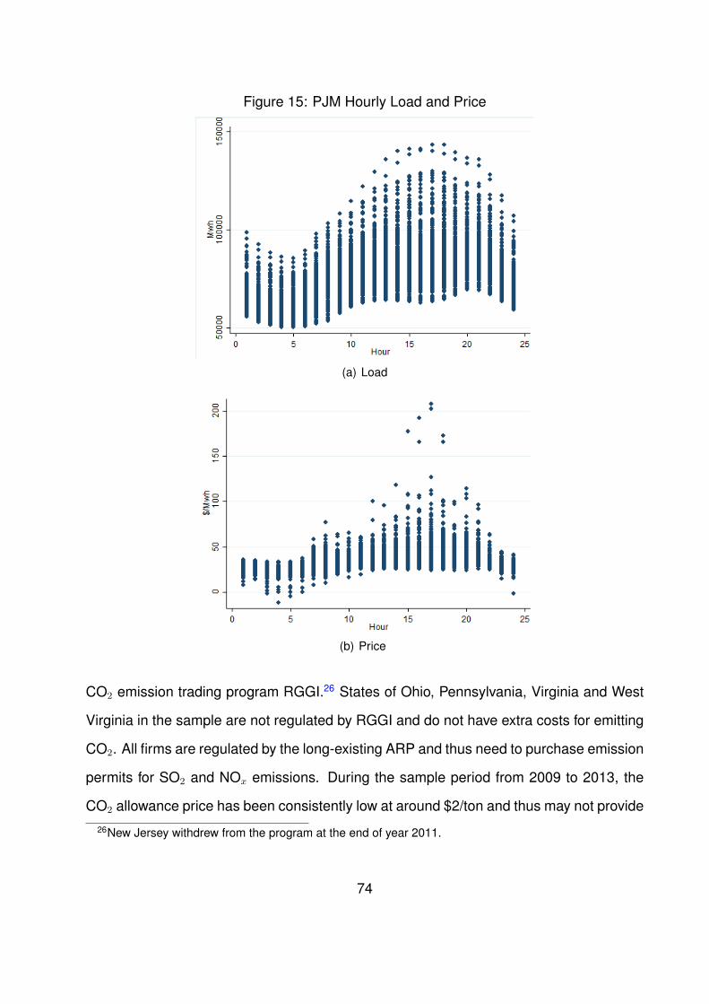
Figure 15: PJM Hourly Load and Price

(a) Load

(b) Price

CO2 emission trading program RGGI.26 States of Ohio, Pennsylvania, Virginia and West

Virginia in the sample are not regulated by RGGI and do not have extra costs for emitting

CO2. All firms are regulated by the long-existing ARP and thus need to purchase emission

permits for SO2 and NOx emissions. During the sample period from 2009 to 2013, the

CO2 allowance price has been consistently low at around $2/ton and thus may not provide26New Jersey withdrew from the program at the end of year 2011.

74

Figure 16: Emission Prices Over Time

(a) SO2 and NOx (b) CO2

enough incentives for firms to make adjustment. The effectiveness of RGGI program has

been long criticized due to its low allowance prices and limited price variation. As a matter

of fact, the annual emission cap in the first control period was loose and allowance price

was at the predetermined price floor (Figure 16). Therefore, whether the carbon price

is sufficiently high and to what extent emissions can be reduced with tighter regulation is

still underexplored. Motivated by this, the paper empirically estimates how individual firms

adjust production (and thus emissions) to various levels of CO2 allowance prices.

I estimate the intertemporal model proposed by Mansur (2008) for each producer sep-

arately. The results validate the findings in Mansur (2008) that both past and future

markups are also related with output decision in the current period. The intertemporal

model predicts actual production better than the static model does, which assumes cur-

rent output only depends on current markup. With the estimated parameters from the

intertemporal model, I examine how each producers’ generation (and thus emissions)

change if a more stringent carbon policy raise the cost of production. The results show

that all other things remain the same, the CO2 emissions decrease as allowance price

increases, but the emission reduction slows down as the permit price of CO2 approaches

$15/ton. For generators located in Delaware and Maryland, the RGGI policy has helped

to decrease the total CO2 emissions by at least 4.73% during the sample period. When

75

the permit price is within the neighborhood of actual data, the reduction in CO2 emissions

due to a $1/ton increase in permit price is 0.304 million tons, or 1.85% of the total CO2

emissions. Emissions can be reduced by 23.50% if carbon is priced at $15/ton.

Fuel switching from coal to natural gas arises as CO2 price increases, i.e., generation

from coal generators decreases and generation from natural gas generators increases.

However, the scale of fuel switching is small due to the limited capacity and generation of

natural gas generators within Delaware and Maryland. I also compare producers’ reac-

tions to higher carbon prices during peak and off-peak hours. When carbon price is rela-

tive low (below $10/ton), the reductions in generation and CO2 are comparable between

peak and off-peak hours. However, as carbon price continues raising, the abatement of

CO2 slows down more in off-peak hours.

The rest of the paper is organized as follows. I introduce the background of RGGI

program in the next section. Section 3 describes a theoretical model of the electricity

market with intertemporal constraints such as start-up cost, ramp rate, capacity and min-

imum load. Section 4 presents the reduced form regression used to empirically estimate

individual generators’ production decisions. Section 5 summarizes the data, and sec-

tion 6 presents regression results of the intertemporal model and predicts generation and

emission responses to different levels of carbon prices. Section 7 concludes.

The RGGI Program

RGGI is a cooperative effort to reduce CO2 emissions among the states of Connecticut,

Delaware, Maine, Maryland, Massachusetts, New Hampshire, New York, Rhode Island,

and Vermont specifically in the electric power sector.27 Regulated sources are fossil fuel-

fired power plants with a capacity of 25 MW or greater located within the RGGI States.

RGGI aims to stabilize and then reduce CO2 emissions within the signatory states. The27See http://rggi.org/rggi.

76

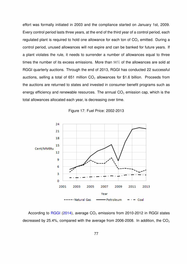
effort was formally initiated in 2003 and the compliance started on January 1st, 2009.

Every control period lasts three years, at the end of the third year of a control period, each

regulated plant is required to hold one allowance for each ton of CO2 emitted. During a

control period, unused allowances will not expire and can be banked for future years. If

a plant violates the rule, it needs to surrender a number of allowances equal to three

times the number of its excess emissions. More than 90% of the allowances are sold at

RGGI quarterly auctions. Through the end of 2013, RGGI has conducted 22 successful

auctions, selling a total of 651 million CO2 allowances for $1.6 billion. Proceeds from

the auctions are returned to states and invested in consumer benefit programs such as

energy efficiency and renewable resources. The annual CO2 emission cap, which is the

total allowances allocated each year, is decreasing over time.

Figure 17: Fuel Price: 2002-2013

According to RGGI (2014), average CO2 emissions from 2010-2012 in RGGI states

decreased by 25.4%, compared with the average from 2006-2008. In addition, the CO2

77

emission rate (pounds of CO2 per megawatt hour) dropped by 16.7%. However, as shown

in Figure 17, natural gas price in the U.S. plummeted during the same period due to the

rapid development of shale gas extraction, led by new applications of hydraulic fracturing

technology and horizontal drilling. This makes natural gas generators more competitive

compared to coal generators, and is a major contributor to the CO2 emission reduction.

Therefore, the effectiveness of RGGI remains questionable and needs to be further ex-

plored.

Although important, RGGI policy is not studied extensively yet. Chen (2009) uses

simulation based on a transmission-constrained electricity market model to address two

issues related to RGGI: CO2 leakage and NOx and SO2 emissions spillover. Shawhan

et al. (2014) model the RGGI regulated plants with a detailed electricity grid. They con-

sider three grid models that have different numbers of transmission nodes. The simulation

results show that impact predictions produced by the model with most nodes differ from

those of the simplified models. Wing and Kolodziej (2009) employ general equilibrium

models to analyze the effectiveness of RGGI. They conclude that RGGI induce power

plants in unconstrained states to generate more electricity and export it to RGGI area,

which results in emission leakage rate of more than 50%. Zhou and Huang (2016) esti-

mate directional distance functions to measure the impact of RGGI on U.S. power plants’

technical efficiency. Ruth et al. (2008) study the impact of participation on the state of

Maryland.

Given that the decrease in natural gas price leads to more use of natural gas gener-

ators which also results in less CO2 emissions, this paper answers the question whether

RGGI is currently effective by analyzing the portion of emission reduction that is attributed

to RGGI carbon pricing with the consideration of intertemporal constraints. In addition, this

paper also contributes to the literature of RGGI by predicting the potential of CO2 reduc-

tion given the characteristics of current regulated fossil fuel generators. The exploration of

both generation and emission responses of individual producers to CO2 allowance price

78

levels not observed in reality also provides insights for policymakers when deciding the

ideal emission cap level.

Electricity Market with Intertemporal Constraints

To illustrate the dynamic decisions in the electricity market, I Follow Mansur (2008) and

Cullen (2015) to construct a profit-maximizing model. The model incorporates dynamic

features of the electricity market into firms’ production decisions. In each hour, firms

maximize the profit given price, cost and intertemporal constraints. I assume firms in PJM

area are price-takers, i.e., they do not strategically manipulate price by altering quantity

of electricity produced, in order to raise profit.

Price taking in electricity market is an important and potentially restrictive assumption,

especially given the extensive studies on market power in electricity markets (Bushnell et

al., 2008b; Holland, 2009; Mansur, 2008; Puller, 2007). However, market power mitigation

actions taken by PJM make this assumption less of a concern, if not perfect. More than

80% of the load is sold in the day-head market, leaving less incentive for firms to raise

price in real-time market. The bids are capped at the reference level to prevent potential

extreme prices. Moreover, a structural screen is performed after bids are submitted in

the day-ahead and real-time markets. PJM implements automatic mitigation of bids from

generating units dispatched for congestion relief if the structural screen is not passed

(Reitzes et al., 2007). In addition, PJM also takes market power mitigation actions in

other markets such as capacity market and ancillary services market. Although there is

occasional local market power as a result of transmission congestion, the overall market

performance is evaluated as competitive (Monitoring Analytics, 2015). The choice of data

also alleviates the concern of market power. I avoid the summer time when demand is at

its peak and firms have the most incentives to exercise market power. Instead, I use data

of each September and October from 2009 to 2013, which approximately represents the

79

average level of demand and generation throughout a year. During the sample period, the

total generation of the firm with the highest aggregate production is only 7.94% of the total

generation of full sample, and the capacity of the largest firm is 4.85% of the aggregate

capacity. 28

With the assumption of price taking, competitive firms maximize profit by maximizing

profit at each generator separately. This is not the case when firms are able to exercise

market power. With market power a firm would consider total production from all genera-

tors that have distinct cost structures. Therefore, throughout the analysis each generator

is regarded as an independent unit maximizing its own profit.

As stated above, Intertemporal constraints such as capacity (CAP ), start-up cost

(START ), ramp rate (R), minimum load (MIN ) impede output adjustment, and make

production decisions in different periods interdependent. These features make the in-

tertemporal model distinct from a "static" model, where generators only care about current

price, and operate at full capacity if price exceeds marginal cost, completely shut down

otherwise. In the "static" model, generators can quickly adjust production with no cost,

the corresponding optimization problem is

Maxqit∈{0,CAPi}

(Pt −mcit) · qit. (15)

where Pt is the electricity price in PJM at time t, andmcit is the marginal cost of production.

I assume each generator has constant marginal cost in each hour, i.e., independent

of production. While the assumption of constant marginal cost might not hold for a firm

or plant that has multiple generators with different characteristics, the marginal genera-

tion cost for a specific physical generating unit is stable. Generator i’s marginal cost of28A firm’s capacity is defined as the largest observed production in an hour.

80

production at time t can be constructed as:

mcit =FuelPrice ∗HeatRateit + SO2Price ∗ SO2Rateit

+NOxPrice ∗NOxRateit + CO2Price ∗ CO2Rateit

(16)

where heat and emission rate are defined as the amount of heat used and pollution emit-

ted in order to produce one megawatt hour (Mwh) of electricity.

By contrast, generating units with non-negligible start-up cost, ramp rate and minimum

load solve a discrete, dynamic decision model. The state variable for generator i in period

t, Sit, is the production level of the previous period

Sit = qit−1

I simplify the process of production adjustment between two periods to a sudden change

at the beginning of each hour, and it is denoted as the choice variable xit: Sit + xit = qit =

Sit+1.

The value function V (Sit), proposed by Mansur (2008), depends on exogenous price

Pt, marginal cost of production mcit, as well as intertemporal variables such as capacity

(CAPi), start up cost (STARTi), ramp rate (Ri) and minimum load (MINi). The Bellman

equation of this dynamic problem can be written as

V (Sit) = Maxxit∈[−Ri,Ri]

{(Pt −mcit) · (Sit + xit)− f(Sit, xit) · STARTi + βV (Sit + xit)

}s.t. : Sit + xit ≥MINi if Sit + xit > 0

and Sit + xit ≤ CAPi,

(17)

where f(Sit, xit) is an indicator variable equals 1 if the generator is turned on from not

81

operating, 0 otherwise:

f(Sit, xit) = 1 if xit > 0 and Sit = 0,

= 0 else.

Note that in the static model maximizing aggregate profit over time is equivalent to

maximizing profit of each period separately, and the production is at full capacity when-

ever price exceeds marginal cost. This however is not the case with the intertemporal

model. With intertemporal constraints generators aim to maximize profit over time by

jointly determine production levels in each period. With a certain level of Sit determined

by past price and limitation imposed by ramp rate, generators may not necessarily be

able to adjust quantity to the level they would have done in the static scenario. Moreover,

in order to achieve a target production level in future periods, they might need to start

increasing or decreasing current output. Therefore, observed quantity of production with

intertemporal constraints could be any number between minimum load and capacity.

Methodology

In the previous section I describe a dynamic model for price taking firms with intertemporal

constraints. However, firms’ expectation of the future path of price needs to be formed

in order to structurally solve the problem (Cullen, 2015). In addition, the calculation of

optimal solution involves extensive computational burden. Instead, this study employs a

reduced form regression developed by Mansur (2008) to empirically investigate how firms’

react to changes in electricity price and marginal cost of production.

With the assumption that firms in PJM behave competitively, each generator can be

regarded as a independent single unit maximizing its own profit. In hour t, generator i’s

82

production, qit, is positively correlated with the current price-cost markup

markupit = Pt −mcit,

where each generator’s marginal cost can be directly calculated from observed heat rate,

fuel price and emission allowance prices. To compare with the static model, a dummy

variable indicating whether the markup is positive (markup_pos) is added to the model.

If the static model fully explains output decisions, then markuppos should be the only

variable which is statistically significant. In addition, as illustrated in the previous section,

generators also take past and future markups into account when choosing qit. This is

mainly due to the existence of intertemporal constraints such as start-up cost and ramp

rate. These constraints make a generator’s production across periods interdependent.

High start-up cost makes generators less willing to change operating status from on

to off, and vice versa. Past markup decides output in past periods, and the past output

level further influences production in current period. For example, if the markup in past

periods is high, the generator was more likely to be operating in the past, and remain

running even with a low current markup, in order to avoid the start up cost. Similarly,

future markup also has an impact on qit. Generators that have a high expectation of

future markup will operate in future periods for sure, thus in current period they might

choose to continue to produce even facing a low current markup, as long as the the loss

from production in current period is less than the start-up cost.

Ramp rate is another intertemporal constraint that makes past and future markups

relevant in deciding current output. Past and future markups are likely to be positively

correlated with past and future production, respectively. With ramp rate, generators’ ability

to adjust quantity is limited, thus how high or low the current production can be depends

heavily on the production level in past periods. Moreover, high future markup provides

incentives for a generator to raise future output. To achieve that target in the future, it

83

might need to start raising production from current period, given that it takes time for a

generator to make adjustment.

To account for these dynamic features, past and future markups are incorporated

into the model. More specifically, I include markups for the past and following hours:

markupit−1 and markupit+1. Furthermore, for generators which are slow to adjust, a high

markupit−1 or markupit+1 itself may not be enough to induce production. For example,

If a generator needs 3 hours to become fully operating from cold status, then it will not

start up knowing that only markup in the following hour (markupit+1) will be high. For this

reason, the average markups of the current (markupit) , previous (markupit−24) and fol-

lowing days (markupit+24) are also included. It is worth noting that although actual future

markup is not yet realized in current period, it is a good proxy for expected future markup

if firms have good knowledge and information of the PJM market. Since the auctions are

repeated on a daily basis, this seems to be a reasonable assumption.

Time-invariant variables such as start-up cost, ramp rate, capacity and minimum load

vary across generators, but can not be separately identified from generator-specific fixed

effects (αi). Moreover, generators respond to various markups differently due to distinct

characteristics. Similar to Mansur (2008), I model each generator’s output decision sepa-

rately. For generator i, the reduced form model is

qit =f(markupit,markupit−1,markupit+1,markupit,markupit−24,markupit+24; βi)

+ αi + γimarkup_posit + εit if qit > 0.(18)

where f(·) is the fifth-order polynomial function and βi is a vector of corresponding

coefficients. The sample included in this regression is a subset of the whole data, which

only includes observations with positive output. The reasons are twofold. First, the com-

prehensive data include many inactive generators which barely operated during sample

period. Moreover, generators with even high aggregate load are not necessarily always

operating, they may switch on and off from hour to hour. Both of the above facts cause the

84

number of observations with zero production to be high. As a matter of fact, the portion

of observations with positive output is only 40.44% of the entire data (Table 14). Includ-

ing many observations with dependent variable at 0 is problematic in an ordinary least

squares regression. The second reason is specific to the electricity market. Due to the

start-up cost, generators need a much higher incentive to raise output from zero to some

positive level. In other words, the increase in markup which causes an output raise from

10 Mwh to 20 Mwh is comparable to that causes a movement from 20 Mwh to 30 Mwh,

which should both be much lower than the markup raise needed to boost production from

0 Mwh to 10 Mwh. For this reason, including observations with zero generation leads to

biased interpretation of the regression results.

Table 14: Number of Observations by Fuel Type

Full Sample qit > 0 Ratio

Coal generators 1,090,656 620,556 56.90%

Natural gas generators 1,137,528 280,605 24.67%

All generators 2,228,184 901,161 40.44%

Another concern is the issue of endogeneity. Since markup is calculated as the gap

between electricity price and marginal cost of production, if either price or marginal cost

could be affected by then output decision, then the estimates are biased. Because of the

assumption of competitive behavior, generators take price as given and cannot influence

electricity price by altering quantities. Equation 18 is regressed at generator level, the

marginal cost of a physical generating unit can be considered as constant in every period.

Heat rate of a generator is also stable once heated up. Therefore, increasing or decreas-

ing production is not likely to have a big impact on marginal cost of a generator. However,

it is worth noting that the assumption of constant marginal cost may not hold at the utility

85

level; The marginal cost of an utility that has multiple generators is a step function.

Data

The majority of generation in PJM Interconnection area is included. More specifically,

the sample contains all firms burning coal or natural gas located in Delaware, Maryland,

Ohio, Pennsylvania, Virginia and West Virginia. I exclude New Jersey from the analysis

as it withdrew from the program at the end of year 2011. Generators using oil as the

primary fuel source are dropped from the analysis due to the limited use. In the sample

generation from oil counts for only 1% of the total fossil fuel generation. Moreover, the

price-cost markup is almost always negative for oil generators due to the high oil price.

Therefore, oil generators are only brought online occasionally to meet retail obligation

during peak load or transmission congestion times.

Spanning from 2009 to 2013, I use hourly detailed data at generator level of every

September and October. The reasons of picking this period rather than summer or winter

are threefold. First, firms’ production activities, such as choices of heat input, generation

are close to year averages in September and October. Therefore, it is a good representa-

tion of firms’ behavior throughout a year. Second, in summer when demand is high, fuel

switching between coal and natural gas might be passive: Firms have to use natural gas

more frequently as coal capacity is well used up. By contrast, the sample in this paper

provides a better study of "voluntary" fuel switching, when demand is moderate and both

coal and natural gas capacities are readily available. Last but not least, an important as-

sumption of this analysis is that firms behave competitively. Firms have more incentives

to raise price and exercise market power when demand is high in summer. This issue is

mitigated with the chosen sample.

Three major datasets are used. The first one is Air Markets Program Data (AMPD)

collected by EPA. AMPD provides hourly, generator-level on heat input, gross generation,

86

fuel and generator type, location and CO2, SO2 and NOx emissions. Net generation is

then approximated as 95% of gross generation. Second, PJM reports hourly electricity

wholesale price and demand.29 The third data source is U.S. Energy Information Admin-

istration (EIA), which reports fuel prices of coal, natural gas. State-specific monthly coal

and natural gas prices are obtained from EIA’s Electric Power Monthly issues. Coal price

is stable and does not have large variation (Figure 17), thus monthly coal price is a good

proxy for daily coal price. Natural gas price varies across time and states, but daily spot

natural gas price is only available at the Henry Hub in Louisiana. I estimate state-specific

daily natural gas prices by comparing monthly average prices of other states to that re-

ported at Henry Hub in Louisiana. Natural gas daily price is available for weekdays only, I

acquire estimates of weekend price by calculating weekday average prices for each week.

Even for generators using the same type of fuel and the same generator operating in

different years, heat rate and emission rate may vary. For this reason, generator-specific

average heat rate and emission rate are calculated for each year. The Acid Rain Program

of EPA regulates all firms in the sample and reports SO2 and NOx prices, while only firms

located in Delaware and Maryland are regulated by RGGI and have extra cost of CO2

emissions. The CO2 allowance price is from RGGI quarterly auctions. The data consist of

344 generators from 78 utilities operating in the PJM area from 2009 to 2013, for a total

of 2,228,184 observations.30

Table 15 reports summary statistics of variables used in regressions and data sources.

During the period from 2009 to 2013, natural gas price has already fallen comparing with

previous years. However, on average natural gas price is still higher than coal price. This

explains why coal is still the dominant fuel choice even though it is dirtier. CO2 emission

rate is much higher than that of SO2 and NOx, but the allowance price is also much lower.

The average hourly wholesale electricity price in PJM is 34.70 $/Mwh. For the generators29The wholesale price and demand from day-ahead and real-time markets are reported separately, I

weight by quantity demanded to get average price.30If an utility has plants in multiple states, I treat them as separate utilities, as they face distinct state-level

regulation policies.

87

Table 15: Summary Statistics

Variables Mean Std. Dev. Source

Coal price ($/MMBtu) 2.74 0.53 EIANatural gas price ($/MMBtu) 4.10 0.93 EIAHeat input (MMBtu) 1178.41 2133.40 EPAGross generation (Mwh) 2.76 5.70 EPACO2 (short ton) 113.67 220.17 EPASO2 (short ton) 0.30 0.98 EPANOx (short ton) 0.10 0.24 EPACO2 price ($/short ton) 2.15 0.34 RGGISO2 price ($/short ton) 21.03 25.17 EPANOx price ($/short ton) 215.13 184.60 EPAPJM hourly price ($/Mwh) 34.70 11.43 PJM

Delaware (%) 1.45 EPAMaryland (%) 7.62 EPAOhio (%) 29.11 EPAPennsylvania (%) 29.11 EPAVirginia (%) 19.05 EPAWest Virginia (%) 13.67 EPA

we include in our sample, the RGGI regulated areas are Delaware and Maryland, which

encompasses 9.07% of the total observations.

Figure 18 plots the distribution of heat input, gross generation and emissions by fuel

type for the observations when generators are operating. No graph for SO2 is included

due to the fact that the volume of SO2 emissions from natural gas generators is almost

negligible, thus the only source of SO2 emissions is coal generators. The data show that

currently coal is still the dominant fossil fuel in this industry: Comparing with coal genera-

tors, natural gas generators are much smaller, with much less heat input, generation and

emissions. This is due to its lower cost so that coal generators are often used to serve

base load and operate almost constantly. Figure 19 shows the total monthly heat input

and gross generation for natural gas and coal generators. Consistent with Figure 18, the

use of coal is about five times as high as the use of natural gas. However, over time there

is fuel switching from coal to natural gas: More electricity is produced from natural gas

88

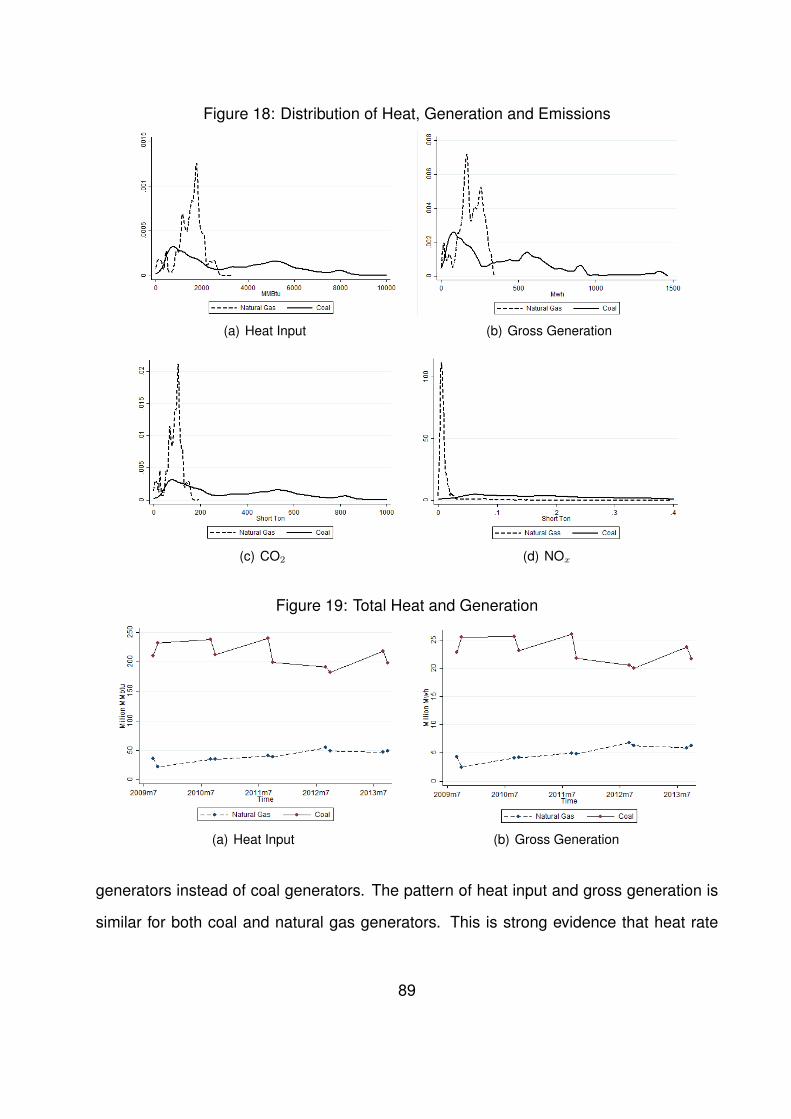
Figure 18: Distribution of Heat, Generation and Emissions

(a) Heat Input (b) Gross Generation

(c) CO2 (d) NOx

Figure 19: Total Heat and Generation

(a) Heat Input (b) Gross Generation

generators instead of coal generators. The pattern of heat input and gross generation is

similar for both coal and natural gas generators. This is strong evidence that heat rate

89

is stable for both types of generators and the assumption of constant marginal cost is

plausible.

Figure 16 illustrates emission allowance prices over time. The allowance prices of

SO2 and NOx have declined significantly. The SO2 price has decreased to a level which is

almost negligible. The price of CO2 allowance price was low and around minimum price

($1.86/ton) between 2010 and 2012, and has increased afterwards. However, the CO2

price level remains low even with the recent increase. As a result, the effectiveness of

RGGI has been widely questioned.

Empirical Analysis

19.1 Regression Results

This section presents the empirical estimation results of Equation 18. As stated above,

only observations with positive outputs are included. Some generators were barely used

during the sample period and are thus dropped from the analysis. In particular, I drop

generators with less than 300 hours of active production. The remaining data consist of

256 generators, for a total of 854,940 observations.

Table 16 reports the summary of coefficients and corresponding standard errors from

256 generator-specific estimations. As expected, the average of coefficients of dummy

variable markup_pos is positive, but only statistically significant for about half genera-

tors. Furthermore, other markups included in the model also have predictive power and

the associated coefficients are significant for many generators. This is strong evidence

that static model is insufficient in explaining production decisions. In practice, firms take

markups in multiple periods into consideration. The average of marginal effects of the six

markups are shown in the last column of Table 16. The marginal effects are calculated

with the estimated parameters and each generator’s specific markup levels. Current and

90

Table 16: Summary of 256 Generator-specific Estimations: Output Decision

Average of Average of # of Significant MarginalVariables Coefficients Std. Dev. Coefficients Effectsfixed effects 228.439 10.550 254markup_pos 3.103 3.873 133markupt 1.366 0.534 148 3.162markupt2 -0.013 0.022 41markupt3a -0.445 0.597 74markupt4b 7.522 8.280 84markupt5c -2.581 4.464 94markupt−1 0.627 0.348 122 0.728markupt−12a 0.678 15.868 69markupt−13a -0.436 0.456 98markupt−14b 6.117 6.632 107markupt−15c -2.674 3.850 115markupt+1 2.517 0.354 224 2.431markupt+12 -0.029 0.017 125markupt+13a -0.570 0.471 140markupt+14a 0.011 0.007 147markupt+15c -4.824 3.860 146markupt -0.324 2.369 155 0.573markupt2 0.335 0.397 126markupt3 -0.053 0.035 143markupt4a 2.172 1.597 140markupt5a 0.018 0.061 147markupt−24 -4.851 2.849 154 0.416markupt−242 0.988 0.470 124markupt−243 -0.087 0.040 130markupt−244a 1.846 1.627 121markupt−245b 59.146 57.419 123markupt+24 -1.370 1.143 141 -1.680markupt+242 -0.715 0.278 128markupt+243 0.276 0.055 148markupt+244a -30.239 5.846 130markupt+245a 1.128 0.224 146a Coefficients are multiplied by 103.b Coefficients are multiplied by 106.c Coefficients are multiplied by 108.

Robust standard errors.Significant at 5% level.

91

the following hour markups have the highest marginal effects, and all the marginal effects

are positive except that of the average markup of the following day, indicating past and

future markups have strong impact on production.

Table 17 illustrates the estimation results by fuel type. Among the 256 generators,

164 are coal generators and 92 are natural gas generators. The coefficients for coal

generators are generally larger than those for natural gas generators due to the larger

size shown in Figure 18. For both groups, most markups have positive relationship with

quantity of production, and current markup and markup in the next hour have the highest

impact. The average markup of current day has a larger impact on coal generators,

while natural gas generators rely more on average markup of the past day when choosing

production level. The estimation results validate the use of intertemporal model over static

model. In this particular industry, production decisions in each period cannot be regarded

as independent, and both past and future periods matter because of the intertemporal

constraints.

19.2 Static vs. Intertemporal

To compare the static and intertemporal model, I obtain utilization rate for each observa-

tion. Utilization rate is defined as the net generation divided by capacity. It measures to

what degree a generator is utilized. The value of utilization is always between 0 and 1, and

thus is comparable across generators with distinct sizes. For all observations, I compute

conditional expectation of utilization rate at various markup levels, E(utilization|markup),

by using the kernel regression. Predicted utilization rate from both static and intertem-

poral models and actual utilization observed in data are all shown in Figure 20. For the

rest of the paper, I include only variables with coefficients significant at 5% level when

calculating fitted value of intertemporal model. To account for production constraints, I

replace predicted output level above capacity by the capacity, and all negative outputs are

replaced by zero.

92

Table 17: Summary of 256 Generator-specific Estimations by Fuel Type: Output Decision164 Coal Generators 92 Natural Gas Generators

Average of Average of # of Significant Marginal Average of Average of # of Significant Marginal

Variables Coefficients Std. Dev. Coefficients Effects Coefficients Std. Dev. Coefficients Effects

fixed effects 278.269 10.550 162 139.605 3.892 92

markup_pos 4.220 3.873 92 1.111 2.666 41

markupt 1.816 0.534 109 4.190 0.565 0.338 39 1.329

markupt2 -0.017 0.022 23 -0.006 0.016 18

markupt3a -0.628 0.597 56 -0.119 0.352 18

markupt4b 10.560 8.280 64 2.106 3.056 20

markupt5c -3.596 4.464 73 -0.770 0.867 21

markupt−1 0.905 0.348 86 0.892 0.132 0.220 36 0.436

markupt−12a 2.562 15.870 44 -2.680 25

markupt−13a -0.657 0.456 71 -0.040 0.286 27

markupt−14b 9.099 6.632 74 0.801 2.726 33

markupt−15c -4.011 3.850 75 -0.290 0.821 40

markupt+1 3.181 0.354 153 3.071 1.335 0.220 71 1.291

markupt+12 -0.029 0.017 73 -0.029 0.012 52

markupt+13a -0.987 0.471 92 0.172 0.286 48

markupt+14b 17.000 7.000 109 0.042 2.520 38

markupt+15c -7.307 3.860 110 -0.397 0.705 36

markupt 0.111 2.369 105 1.270 -1.099 0.704 50 -0.670

markupt2 0.487 0.397 94 0.064 0.097 32

markupt3 -0.085 0.035 115 0.003 0.009 28

markupt4a 3.641 1.597 113 -0.448 0.346 27

markupt5a 0.025 0.061 111 0.005 0.009 36

markupt−24 -7.150 2.849 111 0.036 -0.752 0.701 43 1.094

markupt−242 1.504 0.470 93 0.067 0.097 31

markupt−243 -0.135 0.040 98 -0.001 0.010 32

markupt−244a 2.798 1.627 97 0.150 0.455 24

markupt−245b 88.483 57.419 93 6.849 10.165 30

markupt+24 -2.138 1.143 104 -0.898 -0.002 0.465 37 -3.073

markupt+242 -1.101 0.278 100 -0.027 0.067 28

markupt+243 0.430 0.055 108 0.001 0.005 40

markupt+244a -47.173 5.846 100 -0.053 0.153 30

markupt+245a 1.759 0.224 99 0.002 0.004 37

a Coefficients are multiplied by 103.b Coefficients are multiplied by 106.c Coefficients are multiplied by 108.

Robust standard errors.Significant at 5% level.

In the sample, 99% of the markups range from -$50/Mwh to $100/Mwh. As markup

increases, the expectation of utilization rate increases from 0.4 to around 0.9. Note that

93

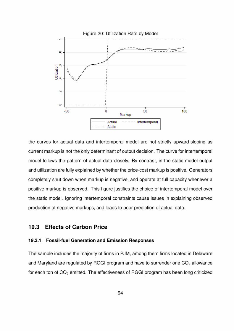
Figure 20: Utilization Rate by Model

the curves for actual data and intertemporal model are not strictly upward-sloping as

current markup is not the only determinant of output decision. The curve for intertemporal

model follows the pattern of actual data closely. By contrast, in the static model output

and utilization are fully explained by whether the price-cost markup is positive. Generators

completely shut down when markup is negative, and operate at full capacity whenever a

positive markup is observed. This figure justifies the choice of intertemporal model over

the static model. Ignoring intertemporal constraints cause issues in explaining observed

production at negative markups, and leads to poor prediction of actual data.

19.3 Effects of Carbon Price

19.3.1 Fossil-fuel Generation and Emission Responses

The sample includes the majority of firms in PJM, among them firms located in Delaware

and Maryland are regulated by RGGI program and have to surrender one CO2 allowance

for each ton of CO2 emitted. The effectiveness of RGGI program has been long criticized

94

due to its low allowance price. This issue is of particular concern during the sample

period: As shown in Figure 16, from 2010 to 2012 the CO2 allowance price was at the

floor ($1.86/ton) due to the loose cap, and the average carbon price is around $2/ton

from 2009 to 2013. Although the CO2 price has increased to around $5/ton recently and

peaked at $7.5/ton in 2015, whether it is sufficiently high and how much emissions can

be reduced with tighter regulation is still underexplored.

To answer this question, I investigate how generators adjust production (and thus

emissions) at various CO2 price levels. Only the 22 generators located in Delaware and

Maryland are included as others are not subject to RGGI regulations. Among the 22

generators, 17 are coal-fired and 5 are natural gas-fired generators. The total number of

observations for RGGI generators is 73,886, which accounts for 8.64% of the full sample.

Markup decreases as CO2 price raises and eventually it is too low so that firms will not

produce and exit in the long run. Therefore, it is unrealistic to set extreme CO2 prices in

practice. Furthermore, when making predictions with estimated parameters, one needs

to be sure that the domain of markups used in the simulation is comparable to that in the

data, otherwise the predictive power of the model is undermined. The relation between

markup and CO2 price is presented in Table 18. As discussed above, observed markups

rage from -$50/Mwh to $100/Mwh, and the average markup is $5.872/Mwh. For the RGGI

area, partly due to the extra cost on carbon, the average markup is -$3.161/Mwh. There-

fore I restrict the range of CO2 price to be under $18/ton, which makes the average markup

to be between -$0.954/Mwh and -$19.521/Mwh for generators located in RGGI area.

Figure 21 plots how aggregate net generation and emissions respond to changes in

CO2 price. At each given CO2 allowance price level, aggregate net generation is obtained

by summing over fitted values of individual observations’ outputs. Along with each gener-

ator’s yearly-specific emission rate, the fitted values of individual outputs are used to con-

struct individual emissions of CO2, SO2 and NOx, respectively. The individual emissions

are then aggregated to get total emissions at each CO2 price level. Note that the response

95

Table 18: Price-cost Markup Under Carbon Pricing in RGGI Area

CO2 Price Average Markup($/ton) ($/Mwh)

0 -0.9541 -1.9862 -3.0173 -4.0494 -5.0805 -6.11210 -11.26915 -16.42620 -21.58330 -31.89840 -42.21350 -52.527

Actual DataFull Sample 5.872RGGI Area -3.161

is not perfectly linear due to the discrepancy of estimated parameters and emission rates

among generators. Moreover, Equation 18 is estimated as fifth-order polynomial function,

thus the marginal effects of carbon price depend on markup levels and vary even for the

same generator across time.

As shown in Figure 21, aggregate net generation in Delaware and Maryland declines

as carbon price raises. The decrease in generation slows down as the permit price of CO2

approaches $15/ton. The response of CO2 shares the similar pattern with the response of

net generation due to the fact that coal is the dominant fuel in RGGI states. Comparison

between coal and natural gas generators will be further explained in the next section.

During the sample period, the average CO2 price is at around $2/ton, and the level of total

CO2 emissions within RGGI area is 16.31 million tons. Without RGGI regulation, total CO2

emissions would have been 17.12 million tons. It is worth noting that observations with

zero production are excluded from the analysis. However, firms may choose to produce in

more periods with the higher markups if there were no CO2 price. Therefore, 17.12 million

tons should be regarded as the lower bound of CO2 emissions without RGGI regulation,

96

Figure 21: Responses to Carbon Pricing in RGGI

(a) Fossil-fuel Generation (b) CO2

(c) SO2 (d) NOx

i.e., the RGGI policy has helped to decrease the total CO2 emissions from RGGI fossil fuel

generators by at least 4.73% during the sample period. When the permit price is within

the neighborhood of actual data, the reductions in net generation and CO2 emissions due

to a $1/ton increase in CO2 price are 0.30 million Mwh and 0.31 million tons, or 1.86% and

1.85% of the total net generation and CO2 emissions, respectively. Although not directly

regulated by RGGI, along with the reduction in fossil fuel generation, the emissions of

SO2 and NOx also decreases with more stringent carbon policy, as shown in Figure 21.

19.3.2 Coal vs. Natural Gas

In the full sample, generation from natural gas is 21.64% of the generation from coal

(Figure 19). However, natural gas generation is only 3.86% of coal generation in the two

97

states regulated by RGGI (Delaware and Maryland). When CO2 allowance price gets

higher, marginal cost of production of both coal and natural gas generators raise, but coal

generators become less competitive than natural gas generators due to the higher emis-

sion rates. As illustrated in Figure 22, generation and CO2 from coal generators decrease

with higher carbon price. However, generation and CO2 from natural gas generators in-

crease with more stringent RGGI policy. This is evidence of fuel switching from coal to

natural gas among fossil-fuel generators. As stated above, coal is still the dominant fuel

in the two states and the scale of fuel switching is small. On average, as the allowance

price raises by $1/ton, CO2 emissions from coal generators decrease by 247.61 thousand

tons, or 1.47% of total CO2 from coal generators. On the other hand, the emissions from

natural generators increase by 0.67 thousand tons, or 0.21% of total CO2 from natural

gas generators.

Although fuel switching from coal to natural gas is observed during the sample period,

the scale is too small to have any meaningful influence. This is primarily due to the limited

natural gas capacity and generation in Delaware and Maryland. The gap between supply

and demand of electricity caused by generation reduction from coal generators could

be filled by generation from energy sources other than fossil fuels , energy efficiency

programs, and import from non-regulated area. However, the estimates provided by this

study are only short run effects. Higher utilization of natural gas generators due to higher

carbon price will lead to new investment in natural gas capacity in the long run.

19.3.3 Peak vs. Off-peak Hours

As indicated by Figure 15, electricity load and price vary significantly during a day, and

generators may respond to carbon pricing differently under distinct market conditions. I

divide sample into two groups: peak hours and off-peak hours. Peak hours are defined

as hour 14 to hour 21, i.e., from 1 PM to 9 PM of each day, and the rest are off-peak

hours. In off-peak hours, only generators with lowest cost of production (usually coal and

98

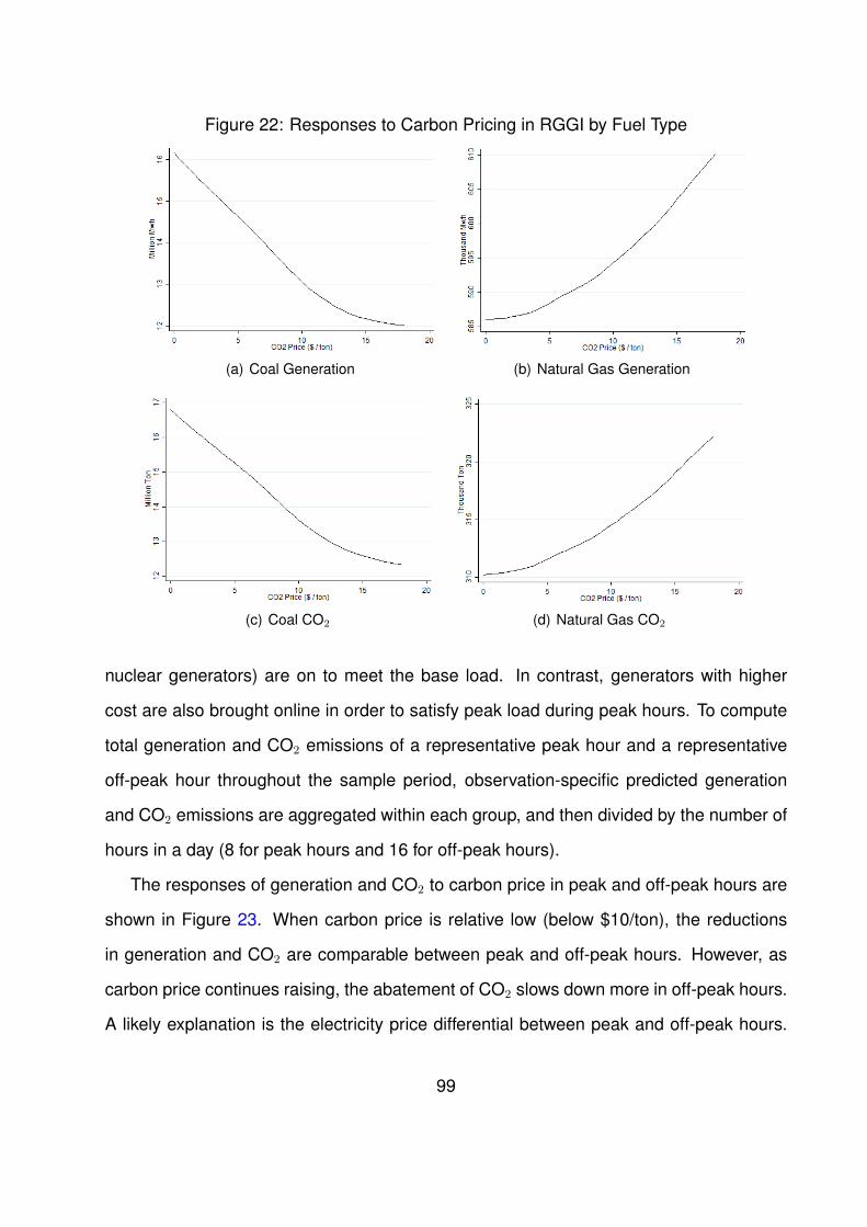
Figure 22: Responses to Carbon Pricing in RGGI by Fuel Type

(a) Coal Generation (b) Natural Gas Generation

(c) Coal CO2 (d) Natural Gas CO2

nuclear generators) are on to meet the base load. In contrast, generators with higher

cost are also brought online in order to satisfy peak load during peak hours. To compute

total generation and CO2 emissions of a representative peak hour and a representative

off-peak hour throughout the sample period, observation-specific predicted generation

and CO2 emissions are aggregated within each group, and then divided by the number of

hours in a day (8 for peak hours and 16 for off-peak hours).

The responses of generation and CO2 to carbon price in peak and off-peak hours are

shown in Figure 23. When carbon price is relative low (below $10/ton), the reductions

in generation and CO2 are comparable between peak and off-peak hours. However, as

carbon price continues raising, the abatement of CO2 slows down more in off-peak hours.

A likely explanation is the electricity price differential between peak and off-peak hours.

99

Producers other than coal and natural gas firms in PJM can be regarded as competitive

fringe suppliers. Generators using other energy sources are likely to be willing to supply

more given higher prices in peak hours, and supply less in off-peak hours when prices are

low. To meet the load obligations, this leaves fossil-fuel generators, especially those using

coal, less room to reduce generation and CO2 emissions even with high carbon price in

off-peak hours.

Figure 23: Fossil-fuel Generation and CO2 in RGGI: Peak vs. Off-peak Hours

(a) Fossil-fuel Generation

(b) CO2

100

19.3.4 Robustness Check

This section tests the robustness of the main results. I use partial data to run the re-

gression Equation 18, then use the estimates to predict firms production in the rest of the

observations. In particular, two robustness checks are performed, with the data of year

2009-2011 and the data of even days only. I examine the predictive power by applying the

estimates to the data of year 2012-2013 and odd days, respectively.

For each regression, I drop observations from generators with less than 300 obser-

vations in the reduced sample. The results are shown in Table 19 and Table 20. Overall

the results are similar to those presented in Table 16. It again validates the important

correlation between production and past and future markups. All markups are statistically

significant for many generators. Most marginal effects are consistent with the main results

except those of average day markups. With the estimates, I compare the predicted kernel

regression of utilization rate with that of the part of actual data not used in the estimation.

As shown in Figure 24, the overall performance of the model is good in predicting utiliza-

tion rate of observations out of the estimation sample. The prediction is very accurate

for low markups ranging from -$50/Mwh to $30/Mwh, but underestimates utilization when

markup gets high.

Conclusion

This paper studies the determinants of electricity firms’ output decisions in a dynamic set-

ting. Consistent with the existing literature, the results validate the use of an intertemporal

model over the static model. Overlooking intertemporal constraints such as start-up cost

and ramp rate leads to biased conclusion, and predicts actual data poorly. The technical

limitations in electricity markets make firms’ output decisions across periods interdepen-

dent. With the estimates of relationship between production and current, past and future

price-cost markups, I investigate the CO2 emission responses to carbon policy which is

101

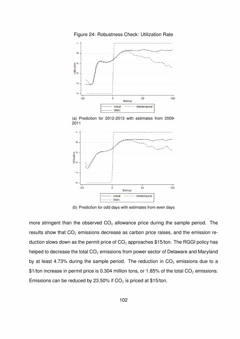
Figure 24: Robustness Check: Utilization Rate

(a) Prediction for 2012-2013 with estimates from 2009-2011

(b) Prediction for odd days with estimates from even days

more stringent than the observed CO2 allowance price during the sample period. The

results show that CO2 emissions decrease as carbon price raises, and the emission re-

duction slows down as the permit price of CO2 approaches $15/ton. The RGGI policy has

helped to decrease the total CO2 emissions from power sector of Delaware and Maryland

by at least 4.73% during the sample period. The reduction in CO2 emissions due to a

$1/ton increase in permit price is 0.304 million tons, or 1.85% of the total CO2 emissions.

Emissions can be reduced by 23.50% if CO2 is priced at $15/ton.

102

Table 19: Robustness Check: Summary of 203 Generator-specific Estimations for 2009-2011

Average of Average of # of Significant MarginalVariables Coefficients Std. Dev. Coefficients Effectsfixed effects 554.443 42.807 200markup_pos 0.636 5.270 97markupt 1.852 0.689 118 5.396markupt2 -0.018 0.027 44markupt3a -1.118 0.976 80markupt4b 0.024 21.500 61markupt5c -0.131 15.400 58markupt−1 0.853 0.465 97 0.700markupt−12a -7.506 21.075 50markupt−13a -0.536 0.766 69markupt−14b 11.700 18.200 57markupt−15c -6.840 14.100 59markupt+1 2.888 0.462 173 2.747markupt+12 -0.032 0.021 108markupt+13a -1.635 0.815 129markupt+14a 0.039 0.019 127markupt+15c -22.200 13.900 108markupt -60.969 11.751 123 -6.640markupt2 9.594 1.919 96markupt3 -0.741 0.160 106markupt4a 25.047 6.657 120markupt5a -0.350 0.142 112markupt−24 -61.946 7.492 113 -0.803markupt−242 10.035 1.235 109markupt−243 -0.787 0.105 109markupt−244a 29.279 4.523 105markupt−245b 382.500 91.000 105markupt+24 -5.556 3.325 127 -0.651markupt+242 0.889 0.614 123markupt+243 -0.055 0.062 124markupt+244a -0.735 4.100 124markupt+245a -0.162 0.174 116a Coefficients are multiplied by 103.b Coefficients are multiplied by 106.c Coefficients are multiplied by 108.

Robust standard errors.Significant at 5% level.

103

Table 20: Robustness Check: Summary of 224 Generator-specific Estimations for EvenDays

Average of Average of # of Significant MarginalVariables Coefficients Std. Dev. Coefficients Effectsfixed effects 248.059 21.281 218markup_pos 0.641 5.514 100markupt 1.656 0.754 111 4.437markupt2 -0.003 0.029 38markupt3a -3.226 0.885 98markupt4b 19.700 14.400 109markupt5c -4.760 9.320 111markupt−1 0.707 0.471 87 0.708markupt−12a -1.773 19.680 44markupt−13a -0.518 0.582 75markupt−14b 8.660 9.140 89markupt−15c -3.140 6.520 100markupt+1 2.788 0.483 198 2.723markupt+12 -0.033 0.021 97markupt+13a -0.645 0.604 121markupt+14a 0.013 0.009 132markupt+15c -4.890 6.970 133markupt 0.382 19.430 115 -0.466markupt2 -0.229 19.765 126markupt3 -0.014 0.067 124markupt4a -0.561 265.121 123markupt5a -0.047 8.411 127markupt−24 -2.607 1.971 122 -1.261markupt−242 0.378 9.997 128markupt−243 -0.009 0.466 130markupt−244a 0.602 0.516 126markupt−245b -27.700 0.046 124markupt+24 -0.010 11.202 118 -0.940markupt+242 -0.077 9.118 122markupt+243 0.072 0.960 120markupt+244a -1.583 0.043 123markupt+245a -0.061 5.991 112a Coefficients are multiplied by 103.b Coefficients are multiplied by 106.c Coefficients are multiplied by 108.

Robust standard errors.Significant at 5% level.

104

Fuel switching from coal to natural gas occurs with carbon pricing. However, the scale

of fuel switching is small due to the limited capacity and generation of natural gas gener-

ators within Delaware and Maryland. When carbon price is relative low (below $10/ton),

the reductions in generation and CO2 are comparable between peak and off-peak hours.

However, as carbon price continues raising, the abatement of CO2 slows down more in

off-peak hours.

There are a few caveats to the analysis that should be noted. First, this paper is a short

run study of carbon effects on firms’ production decisions. In the long run, if CO2 price

is persistently high, existing firms may make investment by adding natural gas capacity

and retiring coal capacity. Carbon regulations can also induce entry/exit if dirtier firms

find it is not profitable to produce and cleaner entrants become more competitive (Cullen,

2015; Ryan, 2012). Second, although the overall PJM market performance is evaluated

as competitive (Monitoring Analytics, 2015), market power could potentially exist in certain

periods. If that is the case, emission reduction resulting from fossil fuel firms strategically

hold production should not be attributed to the carbon regulations. Third, the data used

in the analysis are every September and October from 2009 to 2013. Therefore, one

needs to be cautious when interpreting the estimates of emission response as it may not

well represent firms’ reactions to changes in carbon price during other months, especially

given the fact that both demand and electricity price experience high degree of fluctuations

throughout a year.

105

References

Adair, Sarah K., David C. Hoppock, and Jonas J. Monast, “New Source Review andcoal plant efficiency gains: How new and forthcoming air regulations affect outcomes,”Energy Policy, 2014, 70, 183–192.

Analytics, LLC Monitoring, “State of the Market Report for PJM,” 2015.

Auffhammer, Maximilian and Richard T Carson, “Forecasting the path of China’s CO 2emissions using province-level information,” Journal of Environmental Economics andManagement, 2008, 55 (3), 229–247.

Battese, George E. and Timothy J. Coelli, A Stochastic Frontier Production FunctionIncorporating a Model for Technical Inefficiency Effects Department of Econometrics,University of New England, Armidale. 1993.

Berman, Eli and Linda T. M. Bui, “Environmental Regulation and Productivity: Evidencefrom Oil Refineries,” The Review of Economics and Statistics, 2001, 83 (3), 498–510.

Bovenberg, A Lans, Lawrence H Goulder, and Derek J Gurney, “Efficiency costsof meeting industry-distributional constraints under environmental permits and taxes,”RAND Journal of Economics, 2005, pp. 951–971.

Burtraw, Dallas and Matt Woerman, “Technology Flexibility and Stringency for Green-house Gas Regulations,” 2013. Discussion Paper.

, Joshua Linn, Karen Palmer, and Anthony Paul, “The Costs and Consequences ofClean Air Act Regulation of CO2 from Power Plants,” 2014. Working Paper.

, Karen Palmer, Sophie Pan, and Anthony Paul, “A Proximate Mirror: GreenhouseGas Rules and Strategic Behavior under the US Clean Air Act,” 2015. Working Paper.

Bushnell, James B., Erin T. Mansur, and Celeste Saravia, “Vertical Arrangements,Market Structure, and Competition: An Analysis of Restructured US Electricity Markets,”American Economic Review, 2008, 98 (1), 237–66.

Bushnell, James B, Erin T Mansur, and Celeste Saravia, “Vertical arrangements, mar-ket structure, and competition: An analysis of restructured US electricity markets,” TheAmerican Economic Review, 2008, 98 (1), 237–266.

CCES, “Leveraging Natural Gas to Reduce Greenhouse Gas Emissions,” Technical Re-port, Center for Climate and Energy Solutions 2013.

Chan, Ron, Shanjun Li, and Fan Zhang, “Firm Competitiveness and EU EmissionsTrading System,” Energy Policy, 2013, 63, 1056–1064.

Chen, Yihsu, “Does a regional greenhouse gas policy make sense? A case study ofcarbon leakage and emissions spillover,” Energy Economics, 2009, 31 (5), 667–675.

106

Cole, Matthew A, Robert JR Elliott, Toshihiro Okubo, and Ying Zhou, “The carbondioxide emissions of firms: A spatial analysis,” Journal of environmental economicsand management, 2013, 65 (2), 290–309.

Cullen, Joseph A, “Dynamic Response to Environmental Regulation in the ElectricityIndustry,” 2015.

and Erin T Mansur, “Inferring Carbon Abatement Costs in Electricity Markets: A Re-vealed Preference Approach using the Shale Revolution,” 2015.

Cullenward, Danny and Michael Wara, “Carbon Markets: Effective Policy?,” Science,2014, 344 (6191), 1460.

Ellerman, A. Denny and Juan-Pablo Montero, “The Declining Trend in Sulfur DioxideEmissions: Implications for Allowance Prices,” Journal of Environmental Economicsand Management, 1998, 36, 26–45.

, Paul L. Joskow, Richard Schmalensee, Juan-Pablo Montero, and Elizabeth M.Bailey, Markets for clean air: The US acid rain program, The Press Syndicate of theUniversity of Canbridge, 2000.

Fabra, Natalia and Juan Toro, “Price Wars and Collusion in the Spanish Electricity Mar-ket,” International Journal of Industrial Organization, 2005, 23 (3-4), 155–181.

and Mar Reguant, “Pass-through of emissions costs in electricity markets,” The Amer-ican Economic Review, 2014, 104 (9), 2872–2899.

Färe, Rolf, Shawna Grosskopf, and Carl A Pasurka, “Potential gains from trading badoutputs: The case of US electric power plants,” Resource and Energy Economics, 2014,36 (1), 99–112.

, , C. A. K. Lovell, and Carl Pasurka, “Multilateral productivity comparisons whensome outputs are undesirable: a nonparametric approach,” The Review of Economicsand Statistics, 1989, 71 (1).

, , Carl A Pasurka Jr, and William L Weber, “Substitutability among undesirableoutputs,” Applied Economics, 2012, 44 (1), 39–47.

, , Dong-Woon Noh, and William Weber, “Characteristics of a polluting technology:theory and practice,” journal of Econometrics, 2005, 126 (2), 469–492.

Fleishman, Rachel, Rob Alexander, Stuart Bretschneider, and David Popp, “Doesregulation stimulate productivity? The effect of air quality policies on the efficiency ofUS power plants,” Energy Policy, 2009, 37 (11), 4574–4582.

Godby, Robert, Gregory L Torell, and Roger Coupal, “Estimating the value of additionalwind and transmission capacity in the rocky mountain west,” Resource and EnergyEconomics, 2014, 36 (1), 22–48.

107

Gollop, Frank M. and Mark J. Roberts, “Environmental Regulations and ProductivityGrowth: The Case of Fossil-fueled Electric Power Generation,” Journal of Political Econ-omy, 1983, 91 (4), 654–674.

Greenstone, Michael, John A. List, and Chad Syverson, “The Effects of EnvironmentalRegulation on the Competitiveness of U.S. Manufacturing,” 2012. Working Paper.

Gronberg, Timothy J., Dennis W. Jansen, Lori L. Taylor, and Kevin Booker, SchoolOutcomes and School Costs: A Technical Supplement Texas A&M University 2005.

Hart, Stuart L. and Gautam Ahuja, “Does it pay to be green? An empirical examina-tion of the relationship between emission reduction and firm performance,” Businessstrategy and the Environment, 1996, 5, 30–37.

Hiebert, L. Dean, “The determinants of the cost efficiency of electric generating plants: astochastic frontier approach,” Southern Economic Journal, 2002, pp. 935–946.

Hitaj, Claudia and Andrew Stocking, “Market Efficiency and the U.S. Market for SulfurDioxide Allowances,” January 2014. Working paper.

Holland, Stephen P, “Taxes and trading versus intensity standards: second-best en-vironmental policies with incomplete regulation (leakage) or market power,” TechnicalReport, National Bureau of Economic Research 2009.

Holtz-Eakin, Douglas and Thomas M Selden, “Stoking the fires? CO 2 emissions andeconomic growth,” Journal of public economics, 1995, 57 (1), 85–101.

Huang, Ling and Yishu Zhou, Multiple Price Signals in Carbon Emission Markets Uni-versity of Connecticut 2015.

, Subhash Ray, Kathleen Segerson, and John Walden, Evaluating the Impact of Col-lective Rights-based Fisheries Management: Evidence from the New England Ground-fish Fishery University of Connecticut 2015.

Jaffe, Adam B., Steven R. Peterson, Paul R. Portney, and Robert N. Stavins, “Envi-ronmental Regulation and the Competitiveness of U.S. Manufacturing: What Does theEvidence Tell Us?,” Journal of Economic Literature, 1995, 33 (1), 132–163.

Jha, Akshaya, “Dynamic Regulatory Distortions: Coal Procurement at U.S Power Plants,”March 2015. Working paper.

Joskow, Paul L., Richard Schmalensee, and Elizabeth M. Bailey, “The Marketfor Sul-furDioxide Emissions,” The American Economic Review, 1998, 88 (4), 669–685.

Kossoy, Alexandre and Pierre Guigon, “State and Trends of the Carbon Market 2012,”Technical Report, World Bank 2012.

Linn, Joshua, Erin Mastrangelo, and Dallas Burtraw, “Regulating Greenhouse Gasesfrom Coal Power Plants under the Clean Air Act,” Journal of the Association of Environ-mental and Resource Economists, 2014, 1 (1), 97–134.

108

, , and , “Regulating greenhouse gases from coal power plants under the clean airact,” Journal of the Association of Environmental and Resource Economists, 2014, 1(1/2), 97–134.

Lundy, LLC Sargent &, “Coal-Fired Power Plant Heat Rate Reductions,” Technical Re-port, Chicago: Sargent & Lundy, LLC 2009.

Mansur, Erin T, “Measuring welfare in restructured electricity markets,” The Review ofEconomics and Statistics, 2008, 90 (2), 369–386.

, “Prices versus quantities: environmental regulation and imperfect competition,” Jour-nal of Regulatory Economics, 2013, 44 (1), 80–102.

Matsushita, Kyohei and Fumihiro Yamane, “Pollution from the electric power sector inJapan and efficient pollution reduction,” Energy Economics, 2012, 34 (4), 1124–1130.

McKibbin, Warwick J, Adele C Morris, and Peter J Wilcoxen, “Pricing carbon in theUS: A model-based analysis of power-sector-only approaches,” Resource and EnergyEconomics, 2014, 36 (1), 130–150.

Moullec, Yann Le, “Assessment of carbon capture thermodynamic limitation on coal-fired power plant efficiency,” International Journal of Greenhouse Gas Control, 2012, 7,192–201.

Murray, Brian C, Peter Maniloff, and Evan Murray, “Why Have Greenhouse Emissionsin RGGI States Declined? An Econometric Attribution to Economic, Energy Market,and Policy Factors,” An Econometric Attribution to Economic, Energy Market, and Pol-icy Factors (May 2014). Duke Environmental and Energy Economics Working PaperSeries, No. EE, 2014, pp. 14–01.

Newell, Richard G., William A. Pizer, and Daniel Raimi, “Carbon Market Lessons andGlobal Policy Outlook,” Science, 2014, 343.

Puller, Steven L, “Pricing and firm conduct in California’s deregulated electricity market,”The Review of Economics and Statistics, 2007, 89 (1), 75–87.

Reguant, Mar, “Complementary bidding mechanisms and startup costs in electricity mar-kets,” The Review of Economic Studies, 2014, 81 (4), 1708–1742.

Reitzes, James D, Johannes P Pfeifenberger, Peter Fox-Penner, Gregory NBasheda, José A García, Samuel A Newell, and Adam C Schumacher, “Review ofPJM’s Market Power Mitigation Practices in Comparison to Other Organized ElectricityMarkets,” The Brattle Group, 2007.

RGGI, “CO2 Emissions from Electricity Generation and Imports in the Regional Green-house Gas Initiative: 2012 Monitoring Report,” Technical Report, Regional GreenhouseGas Initiative 2014.

109

Rubin, Jonathan D., “A Model of Intertemporal Emission Trading, Banking, and Borrow-ing,” Journal of Environmental Economics and Management, 1996, 31 (3), 269–286.

Ruth, Matthias, Steven A Gabriel, Karen L Palmer, Dallas Burtraw, Anthony Paul,Yihsu Chen, Benjamin F Hobbs, Daraius Irani, Jeffrey Michael, Kim M Ross et al.,“Economic and energy impacts from participation in the regional greenhouse gas initia-tive: A case study of the State of Maryland,” Energy Policy, 2008, 36 (6), 2279–2289.

Ryan, Stephen P, “The costs of environmental regulation in a concentrated industry,”Econometrica, 2012, 80 (3), 1019–1061.

Shawhan, Daniel L, John T Taber, Di Shi, Ray D Zimmerman, Jubo Yan, Charles MMarquet, Yingying Qi, Biao Mao, Richard E Schuler, William D Schulze et al., “Doesa detailed model of the electricity grid matter? Estimating the impacts of the RegionalGreenhouse Gas Initiative,” Resource and Energy Economics, 2014, 36 (1), 191–207.

Smale, Robin, Murray Hartley, Cameron Hepburn, John Ward, and Michael Grubb,“The impact of CO2 emissions trading on firm profits and market prices,” Climate Policy,2006, 6 (1), 31–48.

Stavins, Robert N., “What Can We Learn from the Grand Policy Experiment? Lessonsfrom SO2 Allowance Trading,” The Journal of Economic Perspectives, 1998, 12 (3),69–88.

, “Chapter 9 – Experience with Market-Based Environmental Policy Instruments,” Hand-book of Environmental Economics, 2003, 1, 355–435.

Sterner, Thomas, Policy Instruments for Environmental and Natural Resource Manage-ment, Resources for the Future, 2003.

Subramanian, Ravi, Sudheer Gupta, and Brian Talbot, “Compliance strategies underpermits for emissions,” Production and Operations Management, 2007, 16 (6), 763–779.

Swinton, John R, “At What Cost dO We Reduce Pollution? Shadow Prices of SOâCCEmissions,” The Energy Journal, 1998, pp. 63–83.

van der Vlist, Arno J., Cees Withagen, and Henk Folmer, “Technical efficiency underalternative environmental regulatory regimes: The case of Dutch horticulture,” Ecologi-cal Economics, 2007, 63 (1), 165–173.

Vollebergh, Herman RJ, Bertrand Melenberg, and Elbert Dijkgraaf, “Identifyingreduced-form relations with panel data: The case of pollution and income,” Journalof Environmental Economics and Management, 2009, 58 (1), 27–42.

Wing, Ian Sue and Marek Kolodziej, “The Regional Greenhouse Gas Initiative: EmissionLeakage and the Effectiveness of Interstate Border Adjustments,” Technical Report,Mimeo 2009.

110

Wolak, Frank A., “An Empirical Analysis of the Impact of Hedge Contracts on BiddingBehavior in a Competitive Electricity Market,” International Economic Journal, 2000, 14(2), 1–39.

Zhang, Ning and Yongrok Choi, “A note on the evolution of directional distance functionand its development in energy and environmental studies 1997-2013,” Renewable andSustainable Energy Reviews, 2014, 33, 50–59.

Zhou, Peng, Ang Beng Wah, and Kim-Leng Poh, “A survey of data envelopment anal-ysis in energy and environmental studies.,” European Journal of Operational Research,2008, 189 (1), 1–18.

Zhou, Yishu and Ling Huang, “Have US power plants become less technically efficient?The impact of carbon emission regulation,” Energy Economics, 2016, 58, 105–115.

111

Appendix A

Table A1: Natural Gas-Only Utilities: Total CapacityVariable Two-year lead log(Zitn) Three-year lead log(Zitn)

(1) (2) (3) (4)Natural gas price a 0.131 0.123 0.098 0.086

(0.115) (0.114) (0.098) (0.097)Electricity price -0.003 -0.003 -0.002 -0.001

(0.003) (0.003) (0.002) (0.002)After -0.048 -0.048 -0.007 -0.004

(0.054) (0.055) (0.045) (0.045)After*RGGI 0.381∗∗∗ 0.371∗∗∗

(0.130) (0.129)CO2 price 0.143∗∗ 0.145∗∗∗

(0.060) (0.054)Trend b 0.104 0.113 -0.001 -0.003

(0.113) (0.115) (0.098) (0.096)CHP 0.157∗ 0.107 0.107 0.076

(0.093) (0.072) (0.089) (0.068)Age -0.003 -0.002 -0.001 -0.001

(0.002) (0.002) (0.001) (0.001)Ownership-Single -0.038∗∗ -0.033∗ -0.022 -0.019

(0.019) (0.018) (0.016) (0.016)Ownership-Other -0.031 -0.025 -0.023 -0.020

(0.021) (0.021) (0.017) (0.017)PJM annual load c -0.029 -0.041 0.041 0.030

(0.128) (0.127) (0.116) (0.116)Constant 7.198∗∗∗ 7.190∗∗∗ 7.139∗∗∗ 7.131∗∗∗

(0.071) (0.071) (0.067) (0.067)Utility fixed effects Yes Yes Yes YesR2 0.9848 0.9844 0.9856 0.9855Observations 421 421 379 379a Coefficients are multiplied by 103.b Coefficients are multiplied by 10.c Coefficients are multiplied by 109.

Robust standard errors in parentheses. ***: p < 1%, **: p < 5%, *: p < 10%.

112

Table A2: Natural Gas-Only and Coal-Only Utilities: Utilization RateVariable Natural gas-only log(Uitn) Coal-only log(Uitc)

(1) (2) (3) (4)Natural gas price -0.002∗∗∗ -0.002∗∗∗

(0.000) (0.000)Coal price -0.000 -0.001

(0.001) (0.001)Electricity price 0.029∗∗∗ 0.029∗∗∗ 0.011∗∗∗ 0.011∗∗∗

(0.003) (0.003) (0.001) (0.001)After 0.026 0.022 0.255∗∗∗ 0.257∗∗∗

(0.113) (0.112) (0.068) (0.068)After*RGGI -0.574∗∗∗ -0.813∗∗∗

(0.133) (0.166)CO2 price -0.217∗∗∗ -0.298∗∗∗

(0.051) (0.067)Capacity -0.001∗∗∗ -0.001∗∗∗ -0.001∗∗∗ -0.001∗∗∗

(0.000) (0.000) (0.000) (0.000)Trend 0.000 0.000 -0.075∗∗∗ -0.070∗∗

(0.026) (0.026) (0.029) (0.029)CHP 0.655∗∗ 0.705∗∗∗ 0.678∗∗∗ 0.669∗∗∗

(0.263) (0.255) (0.139) (0.138)Age 0.040∗∗∗ 0.040∗∗∗ -0.050∗ -0.053∗∗

(0.014) (0.014) (0.026) (0.027)Ownership-Single 0.041 0.047 -0.466∗∗∗ -0.468∗∗∗

(0.236) (0.235) (0.120) (0.120)Ownership-Other -0.474∗ -0.468∗ -0.259∗∗ -0.253∗∗

(0.275) (0.275) (0.116) (0.116)PJM monthly load a 13.200∗∗∗ 13.100∗∗∗ 9.760∗∗∗ 9.930∗∗∗

(4.240) (4.240) (2.180) (2.180)Feb. -0.030 -0.028 -0.076 -0.072

(0.125) (0.125) (0.046) (0.047)Mar. 0.157 0.158 -0.128∗∗ -0.126∗∗

(0.124) (0.124) (0.055) (0.056)Apr. 0.409∗∗∗ 0.411∗∗∗ -0.226∗∗∗ -0.222∗∗∗

(0.130) (0.130) (0.064) (0.064)May. 0.949∗∗∗ 0.950∗∗∗ -0.310∗∗∗ -0.306∗∗∗

(0.122) (0.122) (0.069) (0.069)Jun. 1.513∗∗∗ 1.514∗∗∗ -0.248∗∗∗ -0.247∗∗∗

(0.115) (0.115) (0.062) (0.062)Jul. 1.716∗∗∗ 1.719∗∗∗ -0.158∗∗∗ -0.158∗∗∗

(0.124) (0.124) (0.045) (0.045)Aug. 1.847∗∗∗ 1.849∗∗∗ -0.154∗∗∗ -0.154∗∗∗

(0.117) (0.117) (0.050) (0.050)Sept. 1.218∗∗∗ 1.216∗∗∗ -0.226∗∗∗ -0.226∗∗∗

(0.117) (0.117) (0.059) (0.059)Oct. 0.442∗∗∗ 0.440∗∗∗ -0.351∗∗∗ -0.350∗∗∗

(0.122) (0.122) (0.074) (0.074)Nov. 0.133 0.136 -0.228∗∗∗ -0.221∗∗∗

(0.122) (0.122) (0.066) (0.066)Dec. 0.213∗ 0.211∗ -0.186∗∗∗ -0.187∗∗∗

(0.122) (0.122) (0.065) (0.065)Constant 4.034∗∗∗ 4.044∗∗∗ 8.481∗∗∗ 8.532∗∗∗

(0.623) (0.623) (0.442) (0.447)Utility fixed effects Yes Yes Yes YesR2 0.5781 0.5781 0.2649 0.2640Observations 6240 6240 5364 5364a Coefficients are multiplied by 109.

Robust standard errors in parentheses. ***: p < 1%, **: p < 5%, *: p < 10%.

113

Table A3: Flexible Utilities: Total CapacityVariable log(Zitn + Zitc)

Two-year lead Three-year lead(1) (2) (3) (4)

Natural gas price a -0.219 -0.239 -0.465 -0.420(0.503) (0.506) (0.530) (0.530)

Coal price -0.000 -0.001 0.001 0.001(0.001) (0.001) (0.001) (0.001)

Electricity price 0.008 0.009 0.003 0.002(0.010) (0.010) (0.009) (0.009)

After 0.169 0.153 -0.070 -0.082(0.227) (0.228) (0.245) (0.243)

After*RGGI -0.134 -0.360(0.179) (0.236)

CO2 price -0.024 -0.136(0.068) (0.096)

t 0.031 0.034 0.043 0.045(0.066) (0.066) (0.062) (0.062)

CHP 0.112 0.094 0.180 0.173(0.094) (0.085) (0.109) (0.106)

Age -0.046∗∗ -0.045∗∗ -0.057∗∗ -0.057∗∗

(0.022) (0.022) (0.023) (0.023)Ownership-Single 0.036 0.043 0.304 0.306

(0.331) (0.331) (0.266) (0.266)Ownership-Other -0.107 -0.093 0.221 0.226

(0.339) (0.339) (0.250) (0.248)PJM annual load b -0.317 -0.335 -0.181 -0.155

(0.532) (0.530) (0.534) (0.531)Constant 10.470∗∗∗ 10.491∗∗∗ 10.639∗∗∗ 10.671∗∗∗

(1.225) (1.224) (1.077) (1.082)Utility fixed effects Yes Yes Yes YesR2 0.9217 0.9214 0.9267 0.9264Observations 163 163 147 147a Coefficients are multiplied by 103.b Coefficients are multiplied by 109.

Robust standard errors in parentheses. ***: p < 1%, **: p < 5%, *:p < 10%.

114

Table A4: Flexible Utilities: Natural Gas and Coal Utilization RateVariable log(Uitn) log(Uitc)

(1) (2) (3) (4)Natural gas price a -0.060∗∗∗ -0.060∗∗∗ 0.002∗∗ 0.002∗∗

(0.010) (0.010) (0.001) (0.001)Coal price 0.020∗∗∗ 0.018∗∗∗ 0.001∗ 0.000

(0.004) (0.003) (0.000) (0.000)Electricity price 0.052∗∗∗ 0.054∗∗∗ 0.004∗∗ 0.004∗∗

(0.014) (0.014) (0.002) (0.002)After -0.391 -0.520 0.395∗∗∗ 0.377∗∗∗

(0.468) (0.467) (0.075) (0.076)After*RGGI -2.486∗∗∗ -0.625∗∗∗

(0.437) (0.076)CO2 price -0.727∗∗∗ -0.206∗∗∗

(0.159) (0.032)Capacity b 0.243∗∗∗ 0.244∗∗∗ -0.002 -0.001

(0.016) (0.016) (0.028) (0.003)t 0.387∗∗∗ 0.420∗∗∗ -0.230∗∗∗ -0.222∗∗∗

(0.105) (0.105) (0.019) (0.019)CHP -2.832∗∗∗ -3.014∗∗∗ -0.753∗∗∗ -0.786∗∗∗

(0.704) (0.686) (0.077) (0.080)Age -0.424∗∗∗ -0.426∗∗∗ 0.036∗∗∗ 0.036∗∗∗

(0.038) (0.038) (0.009) (0.009)Ownership-Single 2.980∗∗∗ 3.009∗∗∗ 0.120 0.125

(0.608) (0.612) (0.105) (0.106)Ownership-Other 5.880∗∗∗ 6.020∗∗∗ 0.429∗∗∗ 0.453∗∗∗

(0.825) (0.828) (0.115) (0.116)PJM monthly load c -3.150∗ -3.140∗ 1.420∗∗∗ 1.420∗∗∗

(1.750) (1.750) (0.225) (0.225)Feb. -0.661 -0.631 0.006 0.014

(0.475) (0.477) (0.068) (0.068)Mar. -0.631 -0.604 -0.025 -0.018

(0.471) (0.473) (0.068) (0.069)Apr. -0.782 -0.738 -0.115 -0.104

(0.506) (0.509) (0.070) (0.071)May. -0.283 -0.235 -0.164∗∗ -0.153∗∗

(0.489) (0.491) (0.068) (0.068)Jun. 0.459 0.478 -0.082 -0.076

(0.459) (0.461) (0.065) (0.066)Jul. 0.343 0.353 -0.091 -0.085

(0.500) (0.502) (0.070) (0.071)Aug. 0.449 0.461 -0.098 -0.093

(0.475) (0.477) (0.069) (0.070)Sept. -0.017 -0.007 -0.110∗ -0.109∗

(0.464) (0.465) (0.065) (0.065)Oct. -0.689 -0.670 -0.222∗∗∗ -0.219∗∗∗

(0.480) (0.481) (0.071) (0.071)Nov. -0.213 -0.142 -0.200∗∗∗ -0.183∗∗∗

(0.461) (0.464) (0.070) (0.070)Dec. 0.157 0.172 -0.204∗∗∗ -0.203∗∗∗

(0.451) (0.453) (0.074) (0.075)Constant -4.987∗∗ -4.438∗ 5.195∗∗∗ 5.307∗∗∗

(2.336) (2.322) (0.511) (0.509)Utility fixed effects Yes Yes Yes YesR2 0.6935 0.6919 0.5581 0.5545Observations 2376 2376 2376 2376a Coefficients are multiplied by 10.b Coefficients are multiplied by 100.c Coefficients are multiplied by 108.

Robust standard errors in parentheses. ***: p < 1%, **: p < 5%, *:p < 10%.

115