Embed Size (px)
Citation preview
Three Essays on Credit Risk with a Special Focus on the
Subprime Financial Crisis
Inaugural-Dissertation zur Erlangung des Grades einesDoktors der Wirtschaftswissenschaften
an derWirtschaftswissenschaftlichen Fakultät der
Universität Passau
Betreuer:
Professor Dr. Niklas Wagner
vorgelegt von:
Bastian Breitenfellner
Passau, September 2012

Tag der Disputation: 10. Juli 2013
Referent: Prof. Dr. Niklas Wagner
Korreferent: Prof. Dr. Oliver Entrop

Acknowledgments
During the completion of this dissertation, I received support from many people to whom I
am especially grateful. In particular, I want to thank Prof. Dr. Niklas Wagner, who supervised
this dissertation and co-authored two of the contained essays. The dissertation is the result of
his eorts to introduce me to the interesting eld of credit risk, many inspiring discussion and
countless comments on my essays. All remaining errors are my own. I want to thank Prof.
Dr. Oliver Entrop for agreeing to act as my second supervisor and his helpful comments at
the Doctoral Colloquium at the University of Passau.
I want to thank my former colleagues at the University of Passau for many fruitful discus-
sions. I am especially grateful to Cristoph Riedel, who made many helpful comments on my
essays and supported my considerably during the nalization of this dissertation. I also want to
thank the participants of the Doctoral Colloquia and the Doctoral Seminars at the University
of Passau, who helped me to improve my work by providing helpful suggestions and hints. I
also want to thank several anonymous reveres for providing helpful comments on my essays
which helped to signicantly improve them.
Finally I want to thank my friends and family, in particular my parents, for supporting me
throughout my whole life and making the person I am today.
i
Contents
List of Tables v
List of Figures vii
1 Preface 1
2 Government Intervention in Response to the Recent Financial Crisis: The
Good into the Pot, the Bad into the Crop 8
2.1 Introduction . . . . . . . . . . . . . . . . . . . . . . . . . . . . . . . . . . . 11
2.2 The Tale of Unlimited Risk Transfer . . . . . . . . . . . . . . . . . . . . . . . 13
2.2.1 Securitization . . . . . . . . . . . . . . . . . . . . . . . . . . . . . . 14
2.2.2 The Market for Credit Protection . . . . . . . . . . . . . . . . . . . . 15
2.3 A Rude Awakening . . . . . . . . . . . . . . . . . . . . . . . . . . . . . . . . 16
2.3.1 The Collapse of Credit Markets . . . . . . . . . . . . . . . . . . . . . 16
2.3.2 The CDS-Domino-Eect . . . . . . . . . . . . . . . . . . . . . . . . . 17
2.3.3 The Drying Up of the Interbank Lending Market . . . . . . . . . . . . 18
2.4 Stabilizing the Financial System - Short Term Government Intervention . . . . 21
2.4.1 Are Rescue Packages Appropriate? . . . . . . . . . . . . . . . . . . . 21
2.4.2 A Formal Illustration of Dierent Means of Government Intervention . 22
2.5 Consequences in the Long Term - Lessons
Learned . . . . . . . . . . . . . . . . . . . . . . . . . . . . . . . . . . . . . . 29
2.5.1 The Future Role of Securitization . . . . . . . . . . . . . . . . . . . . 30
2.5.2 The Role of Internal Risk Management . . . . . . . . . . . . . . . . . 31
2.5.3 Long Term Protability versus Short Term Cash Generation . . . . . . 32
2.6 Conclusion and Outlook . . . . . . . . . . . . . . . . . . . . . . . . . . . . . 32
3 Explaining Aggregate Credit Default Swap Spreads 37
3.1 Introduction . . . . . . . . . . . . . . . . . . . . . . . . . . . . . . . . . . . 39
3.2 Literature Review . . . . . . . . . . . . . . . . . . . . . . . . . . . . . . . . 42
ii
3.3 Characteristics of CDS Contracts and CDS Indices . . . . . . . . . . . . . . . 45
3.3.1 The iTraxx Europe Index Family . . . . . . . . . . . . . . . . . . . . . 45
3.3.2 Index Pricing . . . . . . . . . . . . . . . . . . . . . . . . . . . . . . . 46
3.4 Background . . . . . . . . . . . . . . . . . . . . . . . . . . . . . . . . . . . 46
3.4.1 Spread Modeling . . . . . . . . . . . . . . . . . . . . . . . . . . . . . 46
3.4.2 Implications for our Empirical Investigation . . . . . . . . . . . . . . . 47
3.5 Data . . . . . . . . . . . . . . . . . . . . . . . . . . . . . . . . . . . . . . . 48
3.5.1 iTraxx Spread Data . . . . . . . . . . . . . . . . . . . . . . . . . . . 48
3.5.2 Independent Variables . . . . . . . . . . . . . . . . . . . . . . . . . . 51
3.6 Empirical Analysis . . . . . . . . . . . . . . . . . . . . . . . . . . . . . . . . 55
3.6.1 OLS-Regression Results . . . . . . . . . . . . . . . . . . . . . . . . . 56
3.6.2 Quantile Regression Results . . . . . . . . . . . . . . . . . . . . . . . 64
3.6.3 The Lead-Lag Relationship Between the Market for Credit Risk and the
Stock Market . . . . . . . . . . . . . . . . . . . . . . . . . . . . . . 71
3.7 Conclusion . . . . . . . . . . . . . . . . . . . . . . . . . . . . . . . . . . . . 78
4 The Method of Maximum Implied Default Correlation and its Potential
Applications 83
4.1 Introduction . . . . . . . . . . . . . . . . . . . . . . . . . . . . . . . . . . . 85
4.2 Related Literature . . . . . . . . . . . . . . . . . . . . . . . . . . . . . . . . 87
4.3 Correlated Defaults and Implied Bounds for Default Correlation . . . . . . . . 88
4.4 Incorporating Default Correlation into an Intensity-Based Pricing Framework
for Credit Derivatives . . . . . . . . . . . . . . . . . . . . . . . . . . . . . . 91
4.5 Possible Applications for the Method of Maximum Implied Default Correlation 94
4.5.1 General Methodology . . . . . . . . . . . . . . . . . . . . . . . . . . 94
4.5.2 Deriving Bounds for a CDS Subject to Counterparty Risk . . . . . . . 95
4.5.3 Simulation Results . . . . . . . . . . . . . . . . . . . . . . . . . . . . 96
4.5.4 Pricing Nth-to-Default Baskets . . . . . . . . . . . . . . . . . . . . . 98
4.5.5 Simulation Results . . . . . . . . . . . . . . . . . . . . . . . . . . . . 100
4.6 An Alternative Use: Comparing Dierent Dependence Assumptions . . . . . . 107
4.7 Conclusion . . . . . . . . . . . . . . . . . . . . . . . . . . . . . . . . . . . . 109
4.A The Algorithm of Park and Shin (1998) . . . . . . . . . . . . . . . . . . . . . 114
5 Epilog 117
iii


List of Tables
3.1 Descriptive statistics . . . . . . . . . . . . . . . . . . . . . . . . . . . . . . . 50
3.2 Independent variables included in the econometric model . . . . . . . . . . . . 55
3.3 OLS-regression results for the benchmark index . . . . . . . . . . . . . . . . . 58
3.4 OLS-regression results for the HighVol and the Senior Financials index . . . . . 61
3.5 OLS-regression results for the Subordinated Financials and the Non-nancials
index . . . . . . . . . . . . . . . . . . . . . . . . . . . . . . . . . . . . . . . 62
3.6 Quantile regression results for the benchmark index . . . . . . . . . . . . . . . 65
3.7 Quantile regression results for the HighVol index . . . . . . . . . . . . . . . . 66
3.8 Quantile regression results for the Senior Financials index . . . . . . . . . . . 67
3.9 Quantile regression results for the Subordinated Financials index . . . . . . . . 68
3.10 Quantile regression results for the Non-Financials index . . . . . . . . . . . . . 69
3.11 VARX-regression results for the benchmark index . . . . . . . . . . . . . . . . 72
3.12 VARX-regression results for the HighVol index . . . . . . . . . . . . . . . . . 74
3.13 VARX-regression results for the Senior Financials index . . . . . . . . . . . . . 75
3.14 VARX-regression results for the Subordinated Financials index . . . . . . . . . 76
3.15 VARX-regression results for the Non-Financials index . . . . . . . . . . . . . . 77
4.1 Results for scenario 1 . . . . . . . . . . . . . . . . . . . . . . . . . . . . . . 97
4.2 Results for scenario 2 . . . . . . . . . . . . . . . . . . . . . . . . . . . . . . 97
4.3 Results for scenario 3 . . . . . . . . . . . . . . . . . . . . . . . . . . . . . . 98
4.4 Simulation results for the investment grade scenario . . . . . . . . . . . . . . 101
4.5 Simulation Results for the Non-Investment Grade Scenario . . . . . . . . . . . 103
v

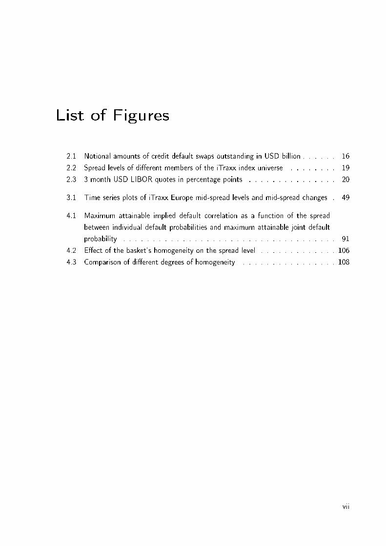
List of Figures
2.1 Notional amounts of credit default swaps outstanding in USD billion . . . . . . 16
2.2 Spread levels of dierent members of the iTraxx index universe . . . . . . . . 19
2.3 3 month USD LIBOR quotes in percentage points . . . . . . . . . . . . . . . 20
3.1 Time series plots of iTraxx Europe mid-spread levels and mid-spread changes . 49
4.1 Maximum attainable implied default correlation as a function of the spread
between individual default probabilities and maximum attainable joint default
probability . . . . . . . . . . . . . . . . . . . . . . . . . . . . . . . . . . . . 91
4.2 Eect of the basket's homogeneity on the spread level . . . . . . . . . . . . . 106
4.3 Comparison of dierent degrees of homogeneity . . . . . . . . . . . . . . . . 108
vii


1 Preface
Crises of dierent magnitude have been part of the nancial services industry since its origin.
However, only few crises, if any, have had the impact of the recent subprime nancial crisis.
After a stage of cheap money pursued by the US Federal Reserve that resulted in a massive
rise of US housing prices, the burst of the consequent bubble triggered widespread distress
throughout banks and insurance companies, which nally distorted the world's economy as a
whole. The current sovereign debt crisis can also be regarded as a direct consequence of the
subprime nancial crisis. Many governments have initiated rescue programs to assist troubled
banks and insurance companies or to prevent their economy from falling into a recession. Due
to their enormous extent, these countermeasures had an massive impact on national budgets.
Additionally, the global economic cooling had a negative eect on national budgets as well.
Besides its enormous impact, what makes the subprime nancial crisis stand out, is its fast
transition over dierent sectors and countries. Having its origin in the US housing market,
the crisis spread quickly and was by no means exclusive to the US or the housing sector. To
give an example, between 01/07/2007 and 04/31/2009, the S&P 500 index dropped by 42%
and the Eurostoxx 50 index, a well-diversied index in Europe, dropped by almost 49 %. The
growing interdependence of nancial markets as a consequence of the ongoing globalization
is one of the reasons for this observations. Others argue that innovations in the nancial
services industry itself favored the quick transition of the crisis throughout dierent sectors.
Among these innovations, the market for credit risk and credit derivatives are particularly under
suspicion.
Credit markets and especially credit derivatives are widely believed to have acted as ac-
celerants during the subprime nancial crisis. The market for credit risk had grown rapidly
before the crisis emerged. It allows to separate the origination of credit risk and bearing the
exposure to such risks, by transferring the risk to a third party. This can be achieved in several
ways. One way is by means of true sale transactions. A bank that grants loans to private
persons or companies, can directly sell the loans to a third party. Another way is by means
of a securitization transaction. In this kind of transaction an originator or a third party that
bought loans in a true sale transaction, pools the loans together and sells securities that are
contingent on the cash ows, the pooled loans generate. A third possible way to transfer
credit risk to a third party is by means of credit derivatives. A bank granting a loan to a large
company can e.g. transfer the credit risk to a third party by insuring against the default of
the company via a credit default swap (CDS) contract or other forms of credit derivatives.
Not only can an originator of credit risk eliminate its exposure to it, third parties with
no expertise in the lending business can obtain exposure to credit risk by the aforementioned
techniques. This is one of the reasons why the subprime nancial crisis was not exclusive to US
2
Savings and Loans Associations, as one might expect, but infected the global nancial services
industry as a whole. Additionally, this circumstance has had an amplifying eect. Since a
broader base of investors had been able to obtain exposure to credit risk, the demand for such
exposure increased signicantly. Therefore, the volume of originated loans and mortgages
increased as well. Nevertheless, as the originators did not have to bare the risk of these loans,
they where not overly concerned with the creditworthiness of their borrowers. This is one of
the reasons why the subprime market grew so rapidly.
Another important issue concerning the recent nancial crisis is the fact that many market
participants underestimated the inherent risks of securitization transactions and credit deriva-
tives, especially for portfolio products, such as nth-to-default baskets and collateralized debt
obligations (CDOs). These products share the common feature that they promise payments,
which are contingent on the solvency of a pool of reference assets. By construction, such
products are very sensitive towards systemic risk, i.e. the joint default of several entities
in their respective reference pool. On the other hand, the pricing models of such products
rely on a joint distribution of defaults for several borrowers, which is highly sensitive towards
the assumptions concerning default dependence. Therefore, underestimating the systemic risk
component, i.e. the default dependence between the reference entities under consideration will
lead to misleading results concerning the risks of portfolio products. Furthermore, the high
complexity of standard models for credit portfolio risk, hampered the assessment of the risks
of structured products, leaving some investors unaware of the actual risk they were exposed
to.
Given the aforementioned setting, it seems natural to investigate the interdependence be-
tween credit markets, credit derivatives and the recent subprime nancial crisis. This investi-
gation is at the core of this dissertation. In particular, it is dedicated to the following research
questions:
• What are the causes of the subprime nancial crisis?
• Which role did credit markets and credit derivatives play during the crisis?
• How might the crisis be resolved?
• What is the impact of the crisis on market participants perception of credit risk?
• How can complex credit derivatives be modeled in a way that allows an understanding
of their inherent risk?
These research questions are addressed in three self-contained essays. The rst essay, co-
authored by Niklas Wagner, is dedicated to examine the causes of the subprime nancial crisis
3
and possible conclusions that can be drawn from it. We discuss instruments such as credit
markets and credit derivatives and how they fostered the instability of the nancial system and
show how the collapse of the nancial system was eventually triggered. Additionally, we discus
possible means of government intervention in oder to resolve the crisis within the nancial
system. We propose a resolution by means of government sponsored purchase programs for
troubled assets. This way of recapitalizing the nancial system has the appealing feature that
it creates a setting, where illiquid, but otherwise solvent, banks are separated from insolvent
banks. Consequently, we address the lessons learned from the subprime nancial crisis by
discussing possible consequences for the design, as well as the regulation of the nancial
system in the future.
The essay adds to the literature on the recent subprime nancial crisis by providing a
thorough discussion of the causes and consequences of the crisis. We put a special focus on
the role of credit markets and credit derivatives as accelerants. Furthermore, we add to the
literature on government intervention by providing a formal illustration of how the design of
government bailout programs can inuence decision making among nancial institutions. For
this purpose, we set up a simple and intuitive model, which helps to illustrate the eects of
typical government bailout programs rather than providing informal arguments in favor of a
certain design. With the help of the model, it can be shown that bailout programs can be
designed in a way such that illiquid but solvent banks behave dierently from insolvent banks.
While not favoring solvent banks in the short run, this provides a valuable signal to outsiders,
including investors as well as government agencies.
The second essay, co-authored by Niklas Wagner, addresses the question how the recent
subprime nancial crisis has altered market participants perceptions concerning the determi-
nants of credit risk, i.e. has the crisis had an impact on the market for credit risk itself? As
the crisis has clearly shown the large vulnerability of the nancial system to systemic risk, one
would expect that market participants have altered their assessment of systematic risk when
pricing credit derivatives. This eect should be particularly pronounced for portfolio products
such as credit indices, as these are, by construction, vulnerable to systemic risk.
To analyze this, we conduct an empirical investigation of the iTraxx Europe index universe
with the recent nancial crisis in focus. We have a special focus on three dierent issues. First,
we analyze the determinants of iTraxx spread changes to learn about the drivers of aggregate
credit risk. We investigate whether the determinants have changed as a consequence of the
recent nancial crisis. If this would have been the case, this would suggest that investors
have adjusted their models of credit risk and have reassessed their assumptions concerning
the systemic component of aggregate credit risk. Second we perform a quantile regression to
4
analyze whether the determinants of iTraxx spreads are suited to explain spread changes in
the upper and lower tail of the empirical distribution, i.e. whether extreme spread changes
are subject to the same factors as changes around the mean or median of the empirical
distribution. Third, we are concerned whether market participants use the iTraxx index as a
source of (additional) information regarding systemic risk. Therefore, we investigate the lead-
lag relationship between the iTraxx index market and equity markets. In case the iTraxx index
market provide valuable information concerning systemic risk, iTraxx spread changes should
not be led by stock market returns.
In order to address the issues outlined above we structure our empirical investigation as
follows. First we examine the determinats of iTraxx spread changes by regressing daily spread
changes of iTraxx Europe index family members on a rich set of explanatory variables. The
set of independent variables comprises factors implied by structural models of credit risk, a
set of liquidity factors and macroeconomic variables. We examine the determinants of the
iTraxx Europe benchmark index, as well as the determinants of the dierent subindices of the
benchmark index. In oder to examine possible changes of the determinants as a consequence of
the recent subprime nancial crisis, we repeat our analysis for dierent subsamples. Our overall
sample ranges from 06/16/2004 to 08/06/2010 and spans the crisis period, as well as a pre-
and a post-crisis period. Hence, we can examine the evolution of credit spread determinants
throughout the nancial crisis. First we estimate our econometric model for the overall sample
and then repeat the estimation for the pre-crisis, crisis and post-crisis subsamples to detect
changes in the set of spread drivers.
In a next step we reestimate our econometric model via a quantile regression. Therefore,
we can examine the performance of our set of explanatory variables in the upper and lower
quantiles of the empirical distribution of spread changes, i.e. to check for the robustness of our
OLS-regression results in dierent quantiles of the empirical distribution of spread changes.
The quantile regression is conducted for all subindices and all subsamples. This allows us
to study the determinants of spread changes in upper and lower quantiles of the empirical
distribution, as well as changes in the determinants in the course of the nancial crisis.
Consequently, to examine whether market participants rely on the iTraxx index as a source of
additional information concerning systemic risk, we examine the lead-lag relationship between
the market for credit risk and stock markets. For this purpose we estimate a vector autore-
gressive model with exogenous variables (VARX-model). The exogenous variables used in the
VARX-model are supposed to jointly determine credit spread changes, as well as stock returns
on a portfolio constructed out of the iTraxx index constituents. We estimate the VARX-model
for all subindices and all respective subsamples to investigate whether the lead-lag relationship
5
has been altered by the recent nancial crisis.
The essay contributes to the existing literature in several ways. First we investigate the
explanatory power of a rich set of independent variables, including proxies for liquidity and
macroeconomic factors. Second, to the best of our knowledge, this is the rst empirical
investigation of the behavior of iTraxx index spreads of the benchmark index and all subindices
with a special focus on changes on credit spread determinants in the course of the recent
subprime nancial crisis. Third, our empirical paper provides deeper insights into the mechanics
of iTraxx spreads by explicitly examining the behavior of credit spread changes at the upper and
lower quantiles of the empirical distribution. Finally, we contribute to the existing literature
by examining the evolution of lead-lag relationships between the iTraxx and stock returns in
the course of the recent nancial crisis, while controlling for several exogenous variables.
In the third essay I address the issue of complexity within portfolio products and credit
derivatives such as nth-to-default baskets and CDSs subject to counterparty risk. During the
recent nancial crisis many of the assumptions behind standard pricing models for portfo-
lio products proved to be myopic. Obviously, many market participants underestimated the
systemic risk component, i. e. the risk associated with the joint default of several entities,
inherent in these portfolio products. Approaches such as the Gaussian copula, which is applied
in latent variable models, do not account for extreme default dependence, i.e. a clustering of
defaults. However, this clustering is a common feature of distressed nancial markets and was
also observed during the recent subprime nancial crisis. Therefore, the market's perception
concerning the inherent risks of portfolio products were not adequate, as common models of
dependent defaults are highly sensitive with respect to assumptions regarding the dependence
structure (Frey and McNeil (2003)).
Models of portfolio credit risk allowing for extreme (possibly asymmetric) dependence of
default are available. However, they are complex and dicult to implement. In this light there
is a pronounced need for concepts allowing to stress test prices of portfolio products, possibly
leading to bounds within the prices (spreads) of such products have to lie in the absence of
arbitrage opportunities and that hold regardless of the actual dependence structures within
the portfolio members. Such concepts allow for a decent understanding of the inherent risk of
portfolio products, as they provide insights concerning the impact of default correlation and
systemic risk on the pricing of such products.
The essay addresses the problem outlined above by introducing the method of maximum
implied default correlation. It contributes to the existing literature by showing that, given the
markets's perception of the stand-alone credit risk of two entities under consideration, it is
possible to derive bounds for the default correlation between them. These bounds hold, as
6

long as no arbitrage opportunities exists. In turn, these bounds can be used to derive upper
and lower bounds for the prices of securities that are subject to credit risk and sensitive to
default correlation via numerical methods. Examples of such securities are credit default swaps
(CDSs) subject to counterparty risk and nth-to-default baskets.
I apply the method of maximum implied default correlation to derive bounds for the prices of
these two types of securities using an intuitive and easy to implement Monte Carlo simulation
algorithm, which is based on a simple intensity model of default. The algorithm involves several
steps. First, implied upper bounds for the default correlation of certain entities are calculated
based on observed market data. Next, the implied upper default correlations are converted
into a variance-covariance matrix of the respective default processes. In a succeeding step
I model the default processes relying on the overlapping sums (OS) method. This involves
expressing the default process of each entity under consideration as a sum of independent
idiosyncratic as well as common default processes. For each entity its respective sum of
default processes is calibrated to match the implied variance-covariance matrix of its default
process. Consequently, the default times of each entity under consideration are simulated,
allowing to derive the upper bound for securities with sensitivity to the default of the entity
under consideration. The respective lower bound can be simulated by assuming that defaults
are independent, i.e. that no default correlation is present. In addition to calculating upper
and lower bounds for nth-to-default baskets and CDSs subject to counterparty risk, I analyze
the sensitivity of the respective spreads concerning changes in the correlation structure of
the underlying entities to provide a better understanding of the potential impact of default
correlation.
The proposed approach allows for the comparison of market spreads for credit derivatives
with model-implied maximum and minimum spreads, without extensive modeling of default
correlations. In the absence of arbitrage opportunities, market quotes have to lie in between
the implied bounds, regardless of the underlying default correlation structure between the
entities contributing to the risk of the security under consideration. Hence, this paper provides
further insights on the impact of default correlation on spreads of credit derivatives sensitive
to default correlation and the eciency of the credit derivatives market as a whole.
7

2 Government Intervention in
Response to the Recent Financial
Crisis: The Good into the Pot, the
Bad into the Crop
Government Intervention in Response to the Subprime
Financial Crisis: The Good into the Pot, the Bad into
the Crop
Bastian Breitenfellner and Niklas Wagner
2010
Published in: International Review of Financial Analysis 19: 289-297
Abstract
The recent global nancial crisis represents a major economic challenge. In order to prevent
such market failure, it is vital to understand what caused the crisis and what are the lessons
to be learned. Given the tremendous bailout packages worldwide, we discuss the role of gov-
ernments as lenders of last resort. In our view, it is important not to suspend the market
mechanism of bankruptcy via granting rescue packages. Only those institutions which are
illiquid but solvent should be rescued, and this should occur at a signicant cost for the re-
spective institution. We provide a formal illustration of a rescue mechanism, which allows
to distinguish between illiquid but solvent and insolvent banks. Furthermore, we argue that
stricter regulation cannot be the sole consequence of the crisis. There appears to be a need
for improved risk awareness, more sophisticated risk management and an alignment of interest
among the participants in the market for credit risk.
9

Keywords: nancial crisis, government intervention, bailout, risk management, credit risk,
credit derivatives, securitization;
10
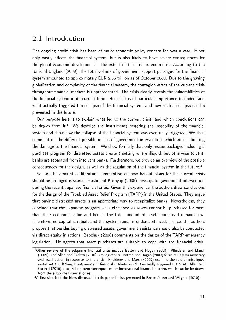
2.1 Introduction
The ongoing credit crisis has been of major economic policy concern for over a year. It not
only vastly aects the nancial system, but is also likely to have severe consequences for
the global economic development. The extent of the crisis is enormous. According to the
Bank of England (2008), the total volume of government support packages for the nancial
system amounted to approximately EUR 5.55 trillion as of October 2008. Due to the growing
globalization and complexity of the nancial system, the contagion eect of the current crisis
throughout nancial markets is unprecedented. The crisis clearly reveals the vulnerabilities of
the nancial system in its current form. Hence, it is of particular importance to understand
what actually triggered the collapse of the nancial system, and how such a collapse can be
prevented in the future.
Our purpose here is to explain what led to the current crisis, and which conclusions can
be drawn from it.1 We describe the instruments fostering the instability of the nancial
system and show how the collapse of the nancial system was eventually triggered. We then
comment on the dierent possible means of government intervention, which aim at limiting
the damage to the nancial system. We show formally that only rescue packages including a
purchase program for distressed assets create a setting where illiquid, but otherwise solvent,
banks are separated from insolvent banks. Furthermore, we provide an overview of the possible
consequences for the design, as well as the regulation of the nancial system in the future.2
So far, the amount of literature commenting on how bailout plans for the current crisis
should be arranged is scarce. Hoshi and Kashyap (2008) investigate government intervention
during the recent Japanese nancial crisis. Given this experience, the authors draw conclusions
for the design of the Troubled Asset Relief Program (TARP) in the United States. They argue
that buying distressed assets is an appropriate way to recapitalize banks. Nevertheless, they
conclude that the Japanese program lacks eciency, as assets cannot be purchased for more
than their economic value and hence, the total amount of assets purchased remains low.
Therefore, no capital is rebuilt and the system remains undercapitalized. Hence, the authors
propose that besides buying distressed assets, government assistance should also be conducted
via direct equity injections. Bebchuk (2008) comments on the design of the TARP emergency
legislation. He agrees that asset purchases are suitable to cope with the nancial crisis,
1Other reviews of the subprime nancial crisis include Batten and Hogan (2009), Peiderer and Marsh(2009), and Allen and Carletti (2010), among others. Batten and Hogan (2009) focus mainly on monetaryand scal action in response to the crisis. Peiderer and Marsh (2009) examine the role of misalignedincentives and lacking transparency in nancial markets, which eventually triggered the crisis. Allen andCarletti (2010) discuss long-term consequences for international nancial markets which can be be drawnfrom the subprime nancial crisis.
2A rst sketch of the ideas discussed in this paper is also presented in Breitenfellner and Wagner (2010).
11

nevertheless he proposes a redesign of the legislation in order to achieve the targets of the
program, i.e. restoring stability in the nancial system, while limiting costs to taxpayers. He
argues that the possibility to overpay for certain assets is not in the interest of taxpayers. In
order to prevent undercapitalization, he rather advocates allowing the purchase of securities
newly issued by troubled institutions. Additionally, he argues that nancial rms should be
required to raise additional capital from their existing shareholders. A potential design of
a government funded asset purchase program is presented by Bebchuk (2009). The author
argues that, rather than setting up a single "Bad Bank", there should be several privately
managed funds which acquire the assets. Their capital should be provided by the government
and by private investors. The fact that several funds compete for the troubled assets assures
that the market for these assets is restored.
Closest to our paper are the papers of Freixas (1999), Gorton and Huang (2004), Diamond
and Rajan (2005), Acharya and Yorulmazer (2008) and Wilson (2010a).
Freixas (1999) compares the costs and benets associated with a bailout of a bankrupt bank.
It is shown that the the optimal bailout policy is determined by the amount of unsecured debt
issued by the respective bank. Nevertheless, the author shows that in equilibrium the lender
of last resort, i.e. the government, will not rescue all banks which have a certain amount of
unsecured debt outstanding, since rescues are costly. Some of these costs are due to moral
hazard at the bank management due to the fact that managers anticipate the chance of being
bailed out. Instead, the lender of last resort optimally follows a mixed bailout strategy, where
she decides case by case whether to rescue a specic bank or not.
Gorton and Huang (2004) claims that the benets of government bailouts depend on the type
of liquidity shock faced by banks. The authors distinguish liquidity shocks from capitalization
shocks. A liquidity shock is an event where banks suddenly need new resources. In contrast,
capitalization shocks stem from a shock to the value of assets on a banks balance sheet.
Government bailouts may be a counterproductive response to banks facing liquidity shocks
as shown by Diamond and Rajan (2002). In case banks face a capitalization shock, Gorton
and Huang (2004) show that government bailouts via asset purchases are feasible, when the
number of assets to be sold is too large to be absorbed by private investors. In this case the
provision of liquidity by the government increases overall welfare.
Acharya and Yorulmazer (2008) provide a formal illustration of the optimal resolution of
bank failures. They show that, in case a suciently large number of banks fail, government
intervention is superior to a private sector resolution of failed banks in terms of social welfare.
They argue that the best way for the government to intervene is through the provision of
liquidity to surviving banks. These funds in turn are used by surviving bank to acquire the
12
assets of failed banks. In contrast to our model, they assume that solvent and insolvent
banks can be separated ex ante. Therefore, their model does not incorporate a mechanism to
distinguish illiquid but solvent and insolvent banks.
A similar approach to ours is followed by Wilson (2010a). The author examines the Public
Private Investment Partnership (PPIP) plan relying on option pricing arguments. In contrast
to our ndings, he concludes, that only solvent banks will be willing to sell distressed assets.3
The reason for the dierent result lies in the fact that the author does not impose an exigent
liquidity need on the banks. Hence, there is no need for the banks to chose the renancing
option which is most favorable for them, as it is the case in our model.
We add to the literature on government intervention by providing a formal illustration of
how the design of government bailout programs can inuence decision making among nancial
institutions. As such, rather than providing informal arguments in favor of a certain design, we
set up a simple and intuitive model, which helps to illustrate the eects of typical government
bailout programs. We show that bailout programs can be designed in a way such that illiquid
but solvent banks behave dierently from insolvent banks. This provides a valuable signal to
outsiders, including investors as well as government agencies.
The remainder of this paper is organized as follows. Section 2.2 briey describes recent
developments in the market for credit risk, which eventually led to the crisis. In Section 2.3,
we discuss why the nancial system broke down and how the crisis spread throughout the
system. Some considerations referring to the use of government bailout programs and our
model are presented in Section 2.4. The lessons learned from the current crisis are discussed
in Section 2.5. Section 2.6 concludes the paper.
2.2 The Tale of Unlimited Risk Transfer
Once upon a time there was a world where banks did not have to bear any risks, as they could
get rid of them in no time. This is an appropriate introduction for a tale about the market for
credit risks. Unfortunately, this is not a tale.
The market for credit risk has grown rapidly since the early 1990's. It seemed to be one of
the biggest success stories in the history of nancial intermediation. The new paradigm was
that underwriting and bearing credit risk could be perfectly separable. As such, credit risk
could be transferred with hardly any constraints by banks to those seeking exposure in certain
credit risks. On the other hand, any player in the nancial system was able to gain exposure
3Wilson (2010b) shows that in some cases even solvent banks might be reluctant to sell toxic assets, as theirshareholders posses an implicit option to put the bank in case of default, which is more valuable if thebank's asset volatility is large.
13
in the credit risk of certain entities, without direct involvement with the respective entity or
even without upfront capital outlays.
The tools for credit risk transfer are numerous, among which Residential Mortgage Backed
Securities (RMBSs) and Credit Default Swaps (CDSs) are the most prominent. The economic
reasoning behind risk transfer is obvious. Financial institutions are able to specialize on certain
segments of the banking landscape. For example, institutions with no expertise in the lending
business are able to gain exposure in any kind of credit risk. On the other hand, originators
are able to eliminate large positions from their books by passing them through to other market
participants. In turn, the relieved capital can be used to grant additional loans. This devel-
opment paves the way for new cash ows to credit markets, allowing the whole economy, as
well as the public to prot from eased funding opportunities, which would not have existed
without the risk transfer. From an economic perspective, it might be questionable whether se-
curitization actually generates additional cash ows to credit markets. Nevertheless, it fosters
an optimal allocation of resources in the credit market, as banks with expertise in the lending
business are best suited to allocate scarce nancial resources among those in need of external
funding.
2.2.1 Securitization
The classic way of transferring credit risk is by means of securitization. In a typical securitiza-
tion transaction, the originator of a credit portfolio sells his credit portfolio to a special purpose
vehicle (SPV), which is renanced via capital markets. Although the assets transferred to the
SPV do no longer occur on the originator's balance sheet, the ties between the originator and
the SPV are manifold, e.g. through swap agreements or guarantees. Securitization transac-
tions have many advantages for the originator. The proceeds from selling the loan portfolio
can readily be used to grant new loans. Therefore, securitization can be regarded as a form
of renancing. Among the other advantages are the transfer of credit risk to the SPV (and
eventually to investors), and lower regulatory capital requirements for the originator.4
Overall, securitization transactions clearly augment lending capacities in the nancial system
and improve allocational eciency of nancial markets concerning both, funds and exposures.
In turn, optimal allocation of resources helps to reduce the cost of credit (see e.g. Due
(2007)). Unfortunately, the number of high quality obligors in the system will be limited.
Hence, the overall proportion of low quality lenders will increase with the volume of lending. At
this point, a disadvantage of securitization becomes obvious. As the originator may eliminate
4Gorton and Souleles (2005) provide a detailed overview of such transactions.
14
all the credit risk associated with the loan portfolio,5 he will not be overly concerned with
the quality of his obligors. Consequently, there will be loans included in the portfolio, which
would not have been granted by the originator, if he still had to account for them. This is
a classic adverse selection problem. The deterioration of the average loan quality is further
amplied by the incentive schemes within the lending business, where employee compensation
largely depends on lending volume rather than on risk-adjusted return (see e.g. Mills and Ki
(2007)).
Additionally, SPVs will typically try to obtain maximal funding from selling securities on
the capital market. In turn, the proceeds are transferred to the originator as a compensation
for acquiring the loan portfolio. Hence, SPVs have an incentive to overstate the quality of
their loan portfolio, again a moral hazard problem, as the investors buying SPV bonds and
commercial papers will typically have an information disadvantage concerning the quality of
the loans contained in the portfolio. The complexity of many securitization transactions adds
to this information asymmetry. The overall quality of the loans underlying the securitization
transaction declines with every new transaction, as the amount of high quality borrowers in the
nancial market is limited. However, the capital inow due to the securitization transaction,
will tempt the originator to grant further loans, despite the lower quality of obligors seeking
debt nancing via loans. These loans are then in turn securitized, creating some sort of vicious
circle.
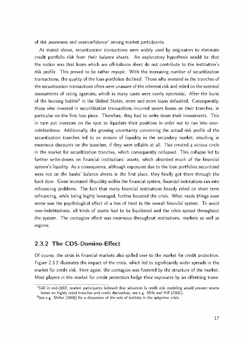
2.2.2 The Market for Credit Protection
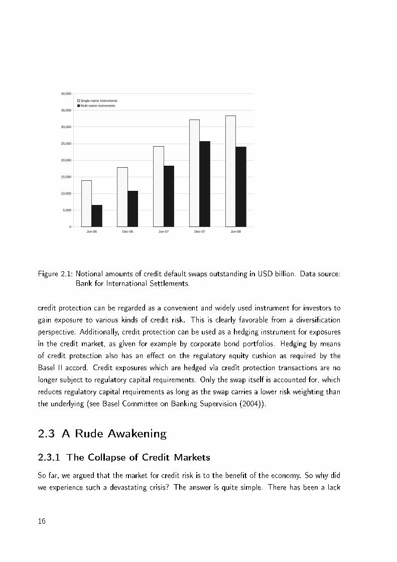
Another segment of the market for credit risk is the market for credit protection. As shown
in Figure 2.2.2, the market for credit protection has grown rapidly in recent years. As of June
2008, it amounted to a total volume of about USD 57.3 trillion of notional principal. Unlike
securitization and credit insurance, buying and selling credit protection in the credit derivatives
market does not require owning the underlying asset. In other words, credit protection is a
synthetic transaction allowing market participants to gain exposure in credit risk with no initial
cash outlay, or without owning the underlying asset.
Among the most common products of the credit protection industry are CDSs and Col-
lateralized Debt Obligations (CDOs).6 Such products compensate the protection buyer for
her losses associated with a credit event related to the underlying asset of the transaction.
Due to the absence of an upfront payment, or the need to actually own the underlying asset,
5At least, this seems to be the case in the rst place. Nevertheless, this is not quite adequate as we discusslater.
6Details on credit derivatives can e.g. be found in Scheicher (2003), who also includes some early warningson nancial stability.
15
0
5,000
10,000
15,000
20,000
25,000
30,000
35,000
40,000
Jun-06 Dec-06 Jun-07 Dec-07 Jun-08
Single-name instruments
Multi-name instruments
Figure 2.1: Notional amounts of credit default swaps outstanding in USD billion. Data source:Bank for International Settlements.
credit protection can be regarded as a convenient and widely used instrument for investors to
gain exposure to various kinds of credit risk. This is clearly favorable from a diversication
perspective. Additionally, credit protection can be used as a hedging instrument for exposures
in the credit market, as given for example by corporate bond portfolios. Hedging by means
of credit protection also has an eect on the regulatory equity cushion as required by the
Basel II accord. Credit exposures which are hedged via credit protection transactions are no
longer subject to regulatory capital requirements. Only the swap itself is accounted for, which
reduces regulatory capital requirements as long as the swap carries a lower risk weighting than
the underlying (see Basel Committee on Banking Supervision (2004)).
2.3 A Rude Awakening
2.3.1 The Collapse of Credit Markets
So far, we argued that the market for credit risk is to the benet of the economy. So why did
we experience such a devastating crisis? The answer is quite simple. There has been a lack
16
of risk awareness and overcondence7 among market participants.
As stated above, securitization transactions were widely used by originators to eliminate
credit portfolio risk from their balance sheets. An explanatory hypothesis would be that
the notion was that loans which are o-balance sheet do not contribute to the institution's
risk prole. This proved to be rather myopic. With the increasing number of securitization
transactions, the quality of the loan portfolios declined. Those who invested in the tranches of
the securitization transactions often were unaware of the inherent risk and relied on the external
assessments of rating agencies, which in many cases were overly optimistic. After the burst
of the housing bubble8 in the United States, more and more loans defaulted. Consequently,
those who invested in securitization transactions incurred severe losses on their tranches, in
particular on the rst loss piece. Therefore, they had to write down their investments. This
in turn put investors on the spot to liquidate their positions in order not to run into over-
indebtedness. Additionally, the growing uncertainty concerning the actual risk prole of the
securitization tranches led to an erosion of liquidity in the secondary market, resulting in
enormous discounts on the tranches, if they were sellable at all. This created a vicious circle
in the market for securitization tranches, which consequently collapsed. This collapse led to
further write-downs on nancial institutions' assets, which absorbed much of the nancial
system's liquidity. As a consequence, although exposures due to the loan portfolios securitized
were not on the banks' balance sheets in the rst place, they nally got there through the
back door. Given increased illiquidity within the nancial system, nancial institutions ran into
renancing problems. The fact that many nancial institutions heavily relied on short term
renancing, while being highly leveraged, further boosted the crisis. What made things even
worse was the psychological eect of a loss of trust in the overall nancial system. To avoid
over-indebtedness, all kinds of assets had to be liquidated and the crisis spread throughout
the system. The contagion eect was enormous throughout institutions, markets as well as
regions.
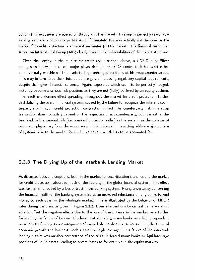
2.3.2 The CDS-Domino-Eect
Of course, the crisis in nancial markets also spilled over to the market for credit protection.
Figure 2.3.2 illustrates the impact of the crisis, which led to signicantly wider spreads in the
market for credit risk. Here again, the contagion was fostered by the structure of the market.
Most players in the market for credit protection hedge their exposures by an osetting trans-
7Still in mid-2007, market participants believed that advances in credit risk modeling would prevent severelosses on highly rated tranches and credit derivatives, see e.g. Mills and Ki (2007).
8See e.g. Shiller (2008) for a discussion of the role of bubbles in the subprime crisis.
17
action, thus exposures are passed on throughout the market. This seems perfectly reasonable
as long as there is no counterparty risk. Unfortunately, this was actually not the case, as the
market for credit protection is an over-the-counter (OTC) market. The nancial turmoil at
American International Group (AIG) clearly revealed the vulnerabilities of the market structure.
Given the setting in the market for credit risk described above, a CDS-Domino-Eect
emerges as follows. In case a major player defaults, the CDS contracts it has written be-
come virtually worthless. This leads to large unhedged positions at his swap counterparties.
This may in turn force them into default, e.g. via increasing regulatory capital requirements,
despite their given nancial solvency. Again, exposures which seem to be perfectly hedged,
instantly become a serious risk position, as they are not (fully) buered by an equity cushion.
The result is a domino-eect spreading throughout the market for credit protection, further
destabilizing the overall nancial system, caused by the failure to recognize the inherent coun-
terparty risk in such credit protection contracts. In fact, the counterparty risk in a swap
transaction does not solely depend on the respective direct counterparty, but it is rather de-
termined by the weakest link (i.e. weakest protection seller) in the system, as the collapse of
one major player may force the whole system into distress. This setting adds a major portion
of systemic risk to the market for credit protection, which has to be accounted for.
2.3.3 The Drying Up of the Interbank Lending Market
As discussed above, disruptions, both in the market for securitization tranches and the market
for credit protection, absorbed much of the liquidity in the global nancial system. This eect
was further emphasized by a loss of trust in the banking system. Rising uncertainty concerning
the nancial health of the banking system led to an increased reluctance among banks to lend
money to each other in the wholesale market. This is illustrated by the behavior of LIBOR
rates during the crisis as given in Figure 2.3.3. Even interventions by central banks were not
able to oset the negative eects due to the loss of trust. Fears in the market were further
fostered by the failure of Lehman Brothers. Unfortunately, many banks were highly dependent
on wholesale funding as a consequence of major balance sheet expansions during the times of
economic growth and business models based on high leverage. This failure of the interbank
lending market was another cornerstone of the crisis. It forced many banks to liquidate large
positions of liquid assets, leading to severe losses as for example in the equity markets.
18
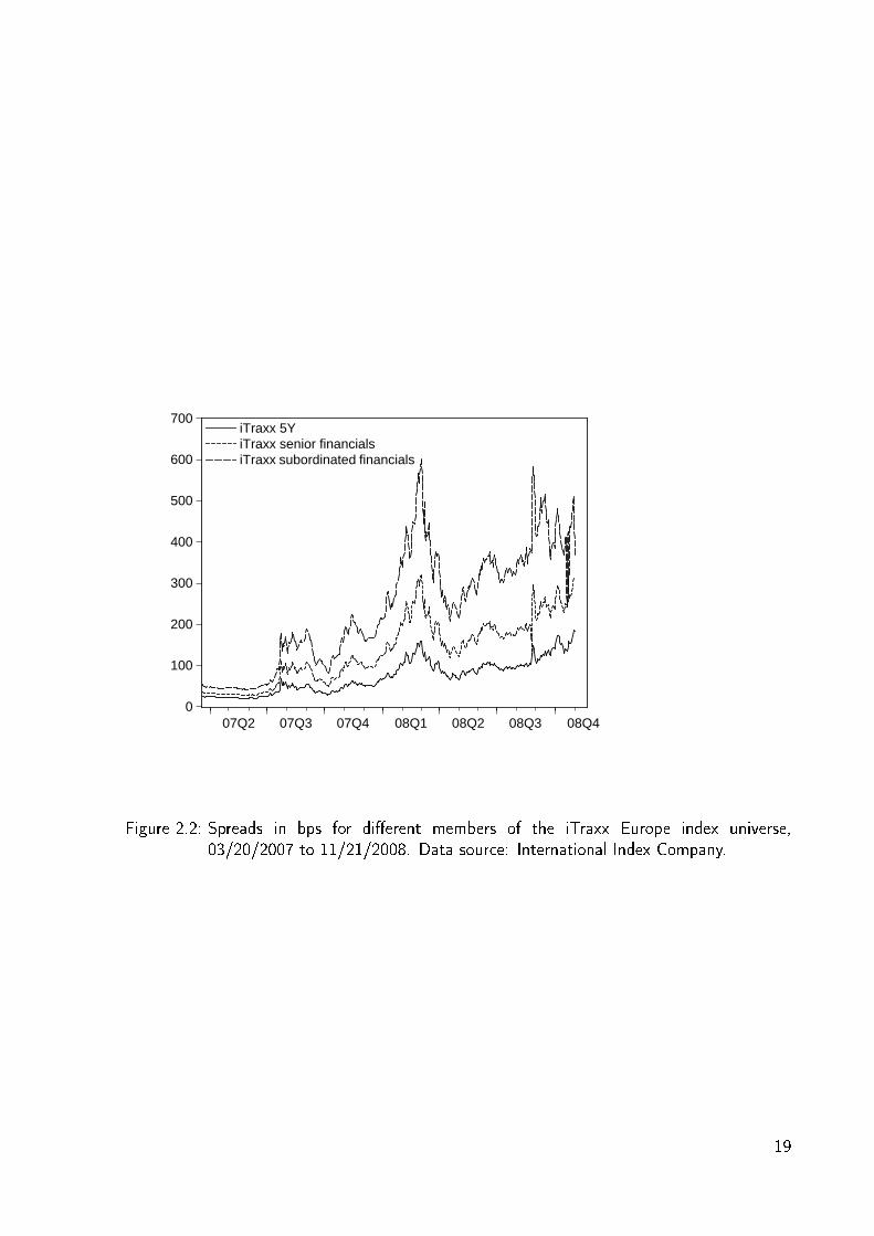
0
100
200
300
400
500
600
700
07Q2 07Q3 07Q4 08Q1 08Q2 08Q3 08Q4
iTraxx 5YiTraxx senior financialsiTraxx subordinated financials
Figure 2.2: Spreads in bps for dierent members of the iTraxx Europe index universe,03/20/2007 to 11/21/2008. Data source: International Index Company.
19
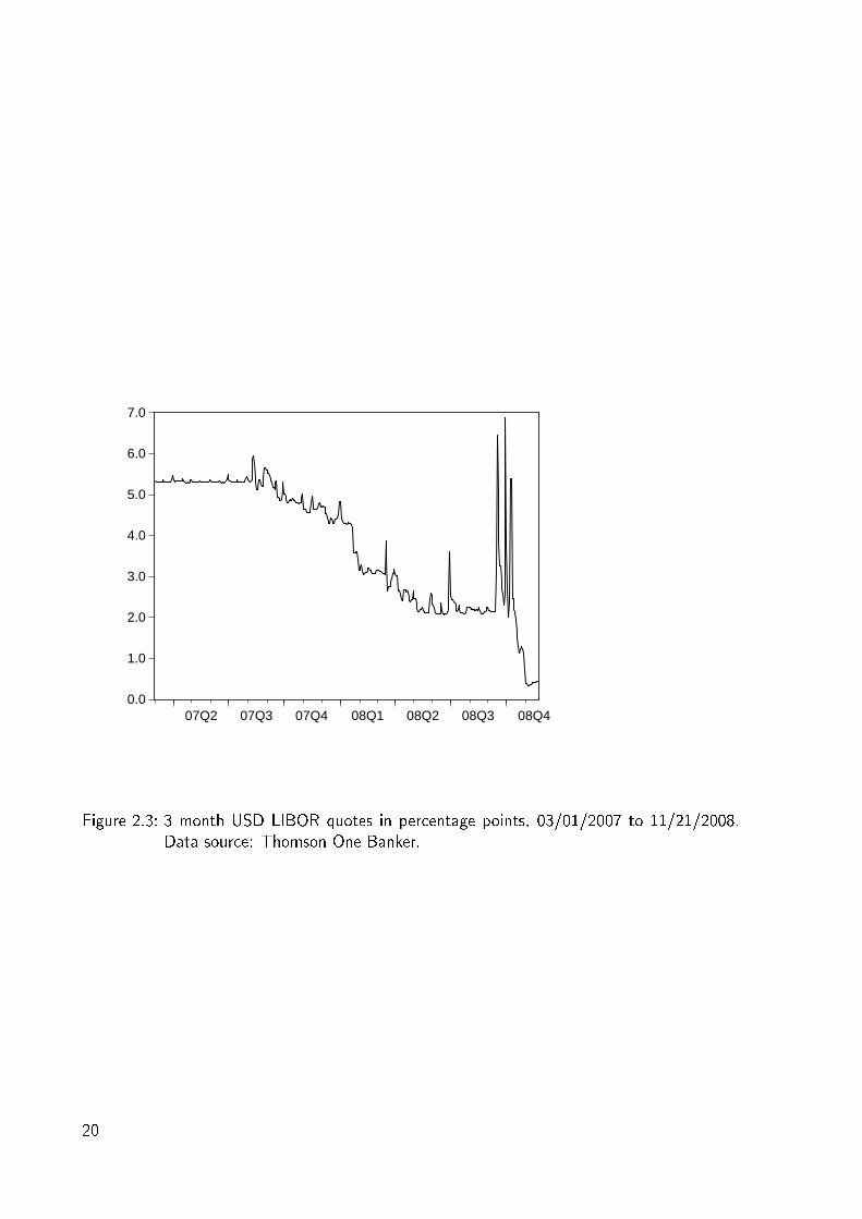
0.0
1.0
2.0
3.0
4.0
5.0
6.0
7.0
07Q2 07Q3 07Q4 08Q1 08Q2 08Q3 08Q4
Figure 2.3: 3 month USD LIBOR quotes in percentage points, 03/01/2007 to 11/21/2008.Data source: Thomson One Banker.
20

2.4 Stabilizing the Financial System - Short Term
Government Intervention
There is no doubt that immediate action has to be taken in order to cope with a crisis of such
magnitude. Otherwise, severe consequences for the nancial system, as well as for the global
economy would be inevitable. Due to the dimension of the subprime crisis, governments seem
to be the only players which can achieve a signicant impact from their interventions. The
general reason behind government intervention and scal policy is subject to ongoing debate
and beyond the scope of this paper. In this section, we focus on the design of short term
government intervention, which aims at stabilizing the nancial system.9
2.4.1 Are Rescue Packages Appropriate?
Governments worldwide have structured rescue packages to support nancial institutions in
distress. This rises an important question: Should distressed nancial institutions be rescued
by the government and consequently by tax payers? On the one hand, rescue measures seem
appropriate given that the bankruptcy costs for the economy would exceed the costs of the
rescue.10 On the other hand, with a government as the lender of last resort, there is little
incentive for nancial institutions to pursue sophisticated risk management strategies. In
contrast, the incentive would be to increase the overall risk prole of the institution in order
to obtain a higher expected payo for shareholders. With a lender of last resort, shareholders
are equipped with a put option written by the government, generating an incentive to increase
the risk prole of the rm at the cost of the government. This again is a classic moral hazard
problem.
In this light, guarantees as sole instrument of government intervention do not seem to
be the appropriate measure to rescue banks. In case a rescue is inevitable, it should be
perused with the help of capital injections rather than guarantees alone in order to avoid
principal agent conicts. Nevertheless, rescue packages should not be used arbitrarily. As
stated above, the presence of a rescue package suspends the important market mechanism
of bankruptcy. This mechanism ensures that only those nancial institutions survive the
crisis, which have pursued sound risk assessment and management. Those institutions with
insucient nancial precautions, in the form of equity buers, should fail in order to ensure
9A long term perspective of government intervention, i.e. deposit insurance, is discussed in Bryant (1980)and Diamond and Dybvig (1983) among others.
10Bankruptcy costs not only comprise direct costs associated with the bankruptcy of a single bank. Addition-ally, the indirect costs of contagion eects within the banking system have to be incorporated, as claimedby Goodfriend and King (1988).
21
the allocational eciency of the nancial system. Therefore, governments should not rescue
nancial institutions, as long as the bankruptcy costs born by the economy do not exceed the
cost of rescue. In case the rescue of a certain nancial institution is inevitable, these measures
of assistance should come at a signicant cost for the respective institution. Otherwise, the
rescue packages could encourage institutions to rely on them as a cheap source of funding.
Given the above, an adequate design of rescue packages appears to be of particular impor-
tance. Among the possible means of government intervention are:
• Government guaranteed debt issuance programs,
• Direct equity injections,
• Purchases of distressed asset by the government.
In general, the design of a government rescue package for the nancial services industry
largely depends on its targets. Among those targets are the stabilization of the nancial
system via recapitalization, taxpayer protection, separation between good and bad management
performance, to name just a few. Unfortunately, some of these targets work in opposite
directions (like recapitalization and tax payer protection). Furthermore, the costs associated
with bank failure are hard to quantify, making it dicult to measure an exact trade-o.
An appropriate rescue package avoids principal agent conicts, while providing immediate
liquidity to institutions which are in the state of distress. Furthermore, the package should only
be to the benet of banks which are illiquid but solvent, or of systemic relevance. At a rst
glance, a superior method to rescue banks is via asset purchases, where nancial institutions
sell with a discount to the economic value of the assets. As the economic value of many of
those assets is above their current market value, this strategy has two major advantages. On
the one hand, only those nancial institutions with severe liquidity problems will be willing
to sell undervalued assets. On the other hand, the government itself can prot from the
expected higher payos from those assets in the future. Nevertheless, banks which need to be
rescued due to their systemic relevance, might not be able to sell distressed assets. Therefore,
combinations of dierent means of recapitalization seem to be necessary.
2.4.2 A Formal Illustration of Dierent Means of Government
Intervention
In this section we formally show how dierent means of government intervention can inuence
decision making within the nancial sector. Our purpose is to illustrate the design of a
rescue package, which allows to distinguish between illiquid but solvent versus insolvent banks.
22
Although this focus might not be in the very best interest of taxpayers in the short run, at
least it allows to identify and reward good management performance. In the long run, this
separation is inevitable for the design of incentive mechanisms, which reward good management
performance. This in turn can prevent future misconduct within the nancial services industry.
In order to illustrate how the dierent means of government rescue packages can inuence
decision making among the nancial services industry, suppose the following setting. There
are two periods. In period t = 0 nancial institutions face a liquidity shortage and decide how
their liquidity need has to be renanced. In t = T the liquidity need vanishes and the capital
obtained in period t = 0 matures. Furthermore, the present value, V0,i, of a future claim is
given by
V0,i = E0[VT,i]e−ri T , (2.1)
where ri is the continuously compounded risk adjusted discount rate for asset i and E0[VT ] is
the time zero expected cash ow due to the claim at maturity.
We next assume that there are two types of banks in the nancial system, good banks and
bad banks, which dier in their default risk. The dierent risk proles of the two types of banks
largely stem from the quality of their balance sheets. Outside investors, including government
authorities, cannot distinguish between the two types, due to information asymmetries.11 The
risk adjusted cost of external funding for good banks is rg and the one for bad banks is rb,
where rg < rb.
Given the probability of ending up with a good bank is pg, 0 < pg < 1 investors will require
a rate of
rl = pgrg + (1− pg)rb (2.2)
for debt capital invested in a bank. Note that, due to asymmetric information, good banks
suer from losses due to higher than necessary renancing costs. To overcome this problem,
they could provide a signal to outside investors and prot from lower renancing rates. How-
ever, as long as bad banks can imitate the signal without incurring signicant costs, the signal
of being either a good or a bad bank is worthless.
Guaranteed Debt Issuance Programs
Suppose now that both types of banks suer from liquidity problems due to a system-wide
nancial crisis and are in need of external debt capital. Both banks can acquire a guarantee for
their debt issuance programs, allowing them to borrow at the risk-free rate rf , where rf < rg.
11This is not a overly restrictive assumption in case the nancial system is in distress. In this case, the focusof the government is more on providing immediate liquidity rather than assessing the risk prole of banksin need of funding.
23
The guarantee comes at a cost at the rate of s, which is the same for both types of lenders, as
the government cannot distinguish between them.12 In this setting, the rate at which a bank
can be renanced is given by
min[pgrg + (1− pg)rb, rf + s]. (2.3)
Banks of both types will rely on the government guarantee as long as the risk-free rate plus the
fee s is lower than their initial renancing costs. This is always true for both banks, since the
good banks cannot provide a credible signal of being in the good cohort. As a consequence,
government support packages will equally favor both types of banks or none of them. In this
case state guarantees are not suited to create a setting where good banks can be separated
from bad ones.
Government assistance in the form of guaranteed debt issuance programs has another im-
portant drawback. As the fee s charged for the state guarantee is a compensation for the
risk of default of the guarantee taker, the government will incur a loss as long as s is too low
relative to the default risk of the guarantee taker. In fact, the government faces the problem
of any other outside investor. Consequently, the fair spread it should charge is given by
s = [pgrg + (1− pg)rb]− rf . (2.4)
The risk-adjusted fee, s, charged for the guarantee is given by the risk-adjusted cost of debt
capital less the risk-free rate. In this setting, the guarantee is either ineective, as it does not
lower the cost of capital for the bank, or it will result in a loss for the government, as the fee
it charges does not cover the expected losses.
Direct Equity Injections
Another way to support distressed nancial institutions is by means of direct equity injections.
This can e.g. be conducted via an increase in share capital, either in the form of common or
preferred stock. The risk adjusted rate of return for preferred stock is rgp for a good bank and
rbp for a bad bank, where rgp < rbp, due to the higher default risk associated with a bad bank.
Accordingly, a good bank is charged a rate of rgc for common equity, and a bad bank is charged
rbc, where rgc < rbc . As equity capital has a lower seniority than debt capital, rg ≤ rgp ≤ rgc
and rb ≤ rbp ≤ rbc must hold. Suppose that the government is willing to obtain preferred or
common shares of a bank. The rate it charges for the equity injection is rf + ip and rf + ic,
12Merton (1977) derives entity specic prices for guarantees using option pricing arguments. However, thisapproach does not seem appropriate for banks, due to the dynamic structure of their assets.
24
respectively, where i represents the risk premium. Again, investors cannot distinguish between
good and bad banks. Thus, any bank can be renanced via preferred shares at a rate of
min[pgrgc + (1− pg)rbp, rf + i], (2.5)
regardless of its risk prole.
The choice between renancing via debt or equity largely depends on the structure of the
respective bank's balance sheet. In general, equity capital is chosen in case the bank aims at
increasing its core capital ratio. In case a bank only seeks for liquidity, as it is otherwise healthy,
it will rather chose to renance via debt capital. Nevertheless, comparing the two possible
cases, it is obvious that the problem faced by banks and investors is nearly the same in both
of them. Both types of banks can renance at the same conditions, regardless of their risk
prole. Additionally, intervention in both cases will either result in a loss for the government
(as long as the risk premium it charges is lower than the expected losses) or, otherwise, it will
be ineective.
Purchases of Distressed Assets
Next suppose that the government, instead of providing guarantees on debt nancing programs,
aims at recapitalizing nancial institutions by buying illiquid assets from their balance sheets.
The purchase of the assets comes at a discount to the (pre-crisis) book value of the assets.
The discount is given by d, d ≥ 0, so the i'th asset is purchased at the time zero price
Pi = Xi(1− d), (2.6)
where Xi is the book value of the asset.
Selling assets to the government has a similar eect on a bank's leverage as being recapital-
ized via an equity injection. Both means of intervention help to decrease the bank's leverage
via increasing its core capital ratio. The dierence between the two lies in the way through
which this decreased leverage is achieved. Asset purchase programs result in reduced balance
sheet totals at the banking sector, while this is not achieved via equity injections.
Combinations of Dierent Means
Most of the government bailout programs launched in the course of the subprime nancial
crisis are a combination of dierent means of government intervention.13 In this section we
13The TARP program is a combination of equity injections and asset distressed asset purchases, while mostEuropean bailout programs combine government guaranteed debt issuance programs with direct equity
25

focus on a combination of debt issuance programs and asset purchases. Nevertheless, our
results generally apply to other combinations as well.
Assume that V0,i is the present value of the expected payo from asset i at maturity. As
long as V0,i ≤ Pi it is rational to sell the asset from the bank's perspective. Furthermore,
for banks with a need for liquidity, selling assets instead of obtaining debt nancing can be
rational even if V0,i ≥ Pi. In any case, the costs of obtaining funding via selling an asset are
given by
V0,i − Pi.
The costs for obtaining external debt nancing amount to
Pi(emin[pgrg+(1−pg)rb, rf+s]T − 1
). (2.7)
In both case we assume a liquidity need of Pi.14 For any bank it is now rational to sell assets
as long as
V0,i − Pi ≤ Pi(emin[pgrg+(1−pg)rb, rf+s]T − 1
). (2.8)
It follows from equation (2.8) that the form of renancing chosen by a bank in our world
depends on the quality of its assets as well as the time horizon of the renancing transaction.
The willingness of the bank to sell assets will decline with a better quality of its assets and a
shorter time horizon of its liquidity needs.
Equilibrium Conditions I
As assumed above, the dierent risk proles of the two types of banks largely stem from
the quality of their balance sheet. The quality of assets held by good banks is likely to be
better than the one of bad banks' assets. Let assets owned by good banks be denoted by
the subscript j and let the ones owned by bad banks carry the subscript k. All banks suer
a liquidity shock and have to obtain liquid funds in order not to default. Both types of banks
face the problem characterized by equation (2.8). Nevertheless, in this setting, the two banks
will behave dierently. As the good banks own high quality assets, they will be reluctant to
sell them and rather chose to be renanced via external debt capital. In contrast, the banks
of the bad cohort will sell a large fraction of their assets.
Furthermore, as the illiquidity of the good banks is caused by a market shock, it is likely to
vanish shortly after its occurrence. Therefore, the time horizon for which good banks have to
injections.14In the special case that the fee equals the fair risk premium, the cost at which any bank may obtain external
funding amounts to Pi(erlT − 1).
26
obtain external capital is short (as they are only subject to the liquidity shock, but otherwise
are solvent). The reverse holds for the bad banks, as their illiquidity is not only due to the
market shock, but also a result of structural issues within the bank.
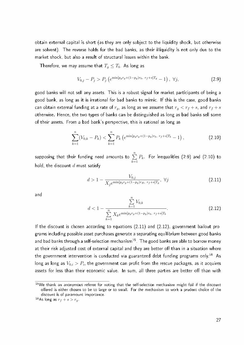
Therefore, we may assume that Tg ≤ Tb. As long as
V0,j − Pj > Pj(emin[pgrg+(1−pg)rb, rf+s]Tg − 1
), ∀j, (2.9)
good banks will not sell any assets. This is a robust signal for market participants of being a
good bank, as long as it is irrational for bad banks to mimic. If this is the case, good banks
can obtain external funding at a rate of rg, as long as we assume that rg < rf + s, and rf + s
otherwise. Hence, the two types of banks can be distinguished as long as bad banks sell some
of their assets. From a bad bank's perspective, this is rational as long as
n∑k=1
(V0,k − Pk) <n∑k=1
Pk(emin[pgrg+(1−pg)rb, rf+s]Tb − 1
), (2.10)
supposing that their funding need amounts ton∑k=1
Pk. For inequalities (2.9) and (2.10) to
hold, the discount d must satisfy
d > 1− V0,jXjemin[pgrg+(1−pg)rB , rf+s]Tg
, ∀j (2.11)
and
d < 1−
n∑k=1
V0,k
n∑k=1
Xkemin[pgrg+(1−pg)rb, rf+s]Tb. (2.12)
If the discount is chosen according to equations (2.11) and (2.12), government bailout pro-
grams including possible asset purchases generate a separating equilibrium between good banks
and bad banks through a self-selection mechanism15. The good banks are able to borrow money
at their risk adjusted cost of external capital and they are better o than in a situation where
the government intervention is conducted via guaranteed debt funding programs only.16 As
long as long as V0,i > Pi, the government can prot from the rescue packages, as it acquires
assets for less than their economic value. In sum, all three parties are better o than with
15We thank an anonymous referee for noting that the self-selection mechanism might fail if the discountoered is either chosen to be to large or to small. For the mechanism to work a prudent choice of thediscount is of paramount importance.
16As long as rf + s > rg.
27

government guarantees only.
Equilibrium Conditions II
In the setting described above, good banks do not hold any assets for which,
V0,j − Pj > Pj(emin[pgrg+(1−pg)rb, rf+s]Tg − 1
). (2.13)
Putting it dierently, we assume that good banks do not hold any distressed assets, which is a
rather restrictive assumption. Nevertheless, this assumption can be relaxed, while we still are
able to separate good and bad banks. This is achieved, as long as selling illiquid assets and
obtaining external debt capital are mutually exclusive.17 In this case, banks are not allowed to
obtain external funding, given that they have sold distressed assets to the government. Good
banks, having a funding need ofm∑j=1
Pj, will not sell any assets as long as
m∑j=1
(V0,j − Pj) >m∑j=1
Pj(emin[pgrg+(1−pg)rb, rf+s]Tg − 1
). (2.14)
Banks will retain assets for which inequality (2.8) holds and they will incur a loss by retaining
assets for which selling is rational. Nevertheless, this loss is outweighed by the loss they would
incur by not being able to rely on external funding, due to the mutual exclusiveness of the two
funding sources. The lower bound for the discount d, for which good banks will be reluctant
to sell any assets, implied by inequality (2.14) is given by
. (2.15)
The upper bound as given by (2.12) remains unchanged. Hence, it can be seen that good and
bad banks still behave dierently in this setting.
A Numerical Example
To illustrate our ndings we provide a small numerical example. Suppose pg = 0.5, rf =
5%, rg = 8%, and rb = 16%. There are two banks, one of either type, which both have a
liquidity need of 100 over the next two months. In the rst case, suppose government assitance
17This can be ensured by restrictive covenants in the purchase agreement. From the government's perspective,this is clearly desirable. Otherwise, banks could use rescue packages as a dump for worthless assets,regardless of their solvency.
28
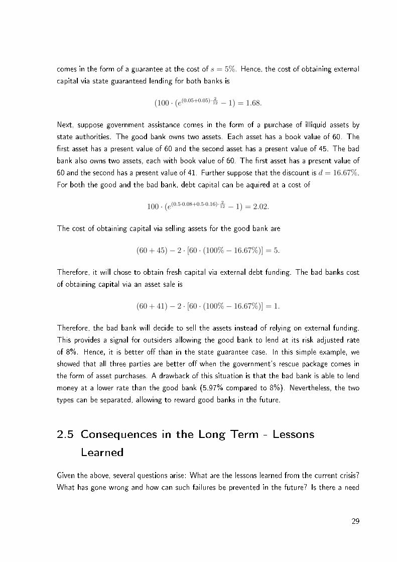
comes in the form of a guarantee at the cost of s = 5%. Hence, the cost of obtaining external
capital via state guaranteed lending for both banks is
(100 · (e(0.05+0.05)· 212 − 1) = 1.68.
Next, suppose government assistance comes in the form of a purchase of illiquid assets by
state authorities. The good bank owns two assets. Each asset has a book value of 60. The
rst asset has a present value of 60 and the second asset has a present value of 45. The bad
bank also owns two assets, each with book value of 60. The rst asset has a present value of
60 and the second has a present value of 41. Further suppose that the discount is d = 16.67%.
For both the good and the bad bank, debt capital can be aquired at a cost of
100 · (e(0.5·0.08+0.5·0.16)· 212 − 1) = 2.02.
The cost of obtaining capital via selling assets for the good bank are
(60 + 45)− 2 · [60 · (100%− 16.67%)] = 5.
Therefore, it will chose to obtain fresh capital via external debt funding. The bad banks cost
of obtaining capital via an asset sale is
(60 + 41)− 2 · [60 · (100%− 16.67%)] = 1.
Therefore, the bad bank will decide to sell the assets instead of relying on external funding.
This provides a signal for outsiders allowing the good bank to lend at its risk adjusted rate
of 8%. Hence, it is better o than in the state guarantee case. In this simple example, we
showed that all three parties are better o when the government's rescue package comes in
the form of asset purchases. A drawback of this situation is that the bad bank is able to lend
money at a lower rate than the good bank (5.97% compared to 8%). Nevertheless, the two
types can be separated, allowing to reward good banks in the future.
2.5 Consequences in the Long Term - Lessons
Learned
Given the above, several questions arise: What are the lessons learned from the current crisis?
What has gone wrong and how can such failures be prevented in the future? Is there a need
29
for stricter regulation in the nancial system? It appears straightforward to blame the nancial
services industry for the crisis and to ask for stricter regulation, but unfortunately, the answer
is not quite as simple as that.
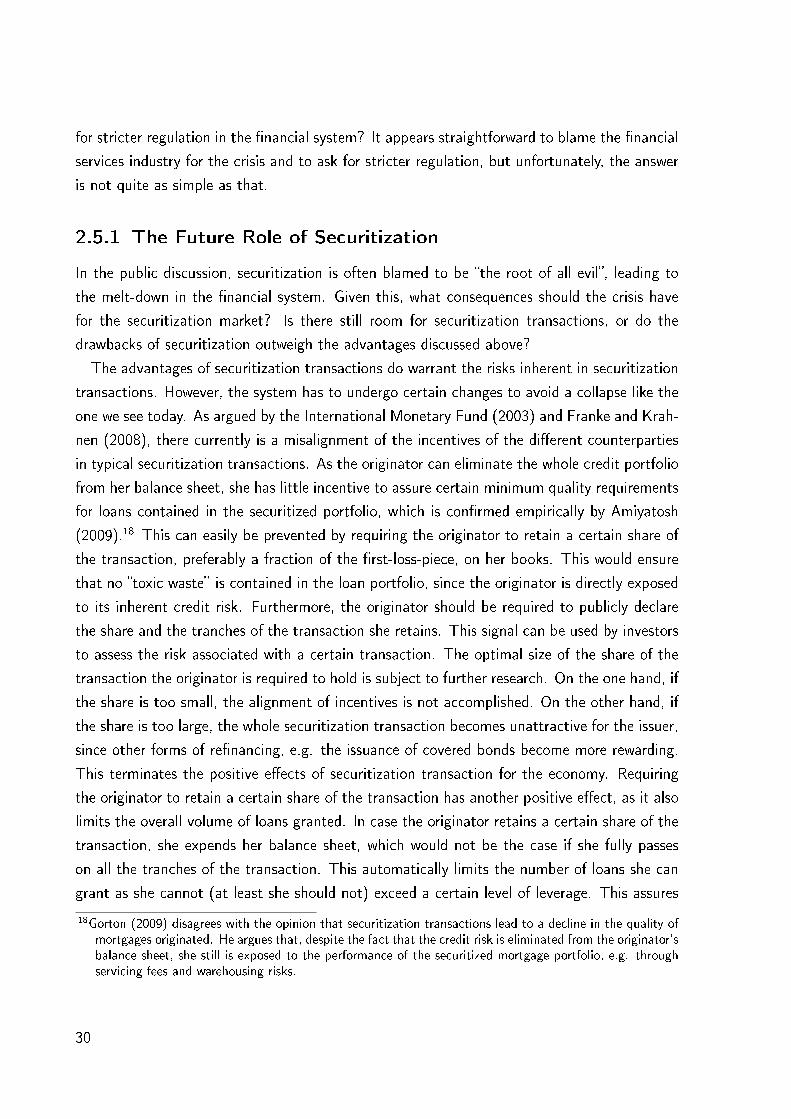
2.5.1 The Future Role of Securitization
In the public discussion, securitization is often blamed to be the root of all evil, leading to
the melt-down in the nancial system. Given this, what consequences should the crisis have
for the securitization market? Is there still room for securitization transactions, or do the
drawbacks of securitization outweigh the advantages discussed above?
The advantages of securitization transactions do warrant the risks inherent in securitization
transactions. However, the system has to undergo certain changes to avoid a collapse like the
one we see today. As argued by the International Monetary Fund (2003) and Franke and Krah-
nen (2008), there currently is a misalignment of the incentives of the dierent counterparties
in typical securitization transactions. As the originator can eliminate the whole credit portfolio
from her balance sheet, she has little incentive to assure certain minimum quality requirements
for loans contained in the securitized portfolio, which is conrmed empirically by Amiyatosh
(2009).18 This can easily be prevented by requiring the originator to retain a certain share of
the transaction, preferably a fraction of the rst-loss-piece, on her books. This would ensure
that no toxic waste is contained in the loan portfolio, since the originator is directly exposed
to its inherent credit risk. Furthermore, the originator should be required to publicly declare
the share and the tranches of the transaction she retains. This signal can be used by investors
to assess the risk associated with a certain transaction. The optimal size of the share of the
transaction the originator is required to hold is subject to further research. On the one hand, if
the share is too small, the alignment of incentives is not accomplished. On the other hand, if
the share is too large, the whole securitization transaction becomes unattractive for the issuer,
since other forms of renancing, e.g. the issuance of covered bonds become more rewarding.
This terminates the positive eects of securitization transaction for the economy. Requiring
the originator to retain a certain share of the transaction has another positive eect, as it also
limits the overall volume of loans granted. In case the originator retains a certain share of the
transaction, she expends her balance sheet, which would not be the case if she fully passes
on all the tranches of the transaction. This automatically limits the number of loans she can
grant as she cannot (at least she should not) exceed a certain level of leverage. This assures
18Gorton (2009) disagrees with the opinion that securitization transactions lead to a decline in the quality ofmortgages originated. He argues that, despite the fact that the credit risk is eliminated from the originator'sbalance sheet, she still is exposed to the performance of the securitized mortgage portfolio, e.g. throughservicing fees and warehousing risks.
30
that the quality of obligors does not decrease arbitrarily.
Another important issue, which led to the nancial crisis is the enormous complexity of
certain products in the market for credit risk. This complexity not only hampered investors'
assessment of the risk associated with the products, even rating agencies were not able to
specify and measure the risk underlying certain transactions. Unfortunately, many investors
relied on external ratings, which were provided by overly optimistic rating agencies. Neverthe-
less, it is astonishing that investors relied on ratings and invested in products they obviously
did not fully understand. The only explanation for this is that sophisticated risk assessment
and management was sacriced on the altar of irrational return expectations.
2.5.2 The Role of Internal Risk Management
The absence of proper risk awareness among market participants is surely among the basic
causes of the current crisis. As argued above, market participants may assume that various
risks can easily be eliminated through instruments like securitization and credit protection.
What has been overseen is the fact that there are risks besides credit risk, which cannot be
eliminated easily, including market risks, liquidity risks, and counterparty risks. The number
of bad loans in the economy does by no means justify the enormous volume of nancial
products which are labeled as toxic waste19during the recent period of market stress. The
essential problem is that there no longer exists a market for these products, due to a lack of
liquidity as well as due to a lack of trust in those products. This fact, in connection with
the fair value accounting principle, causes serious write-downs on investments in those assets,
although these write-downs might only in part be driven by a lack of quality of the product
itself. The possibility of such an erosion of secondary markets has obviously not been taken
into account. This is clearly a failure of internal risk management within nancial institutions.
In this light, one has to discuss the question, whether or not this failure can be prevented
by stricter regulation. A possible solution may be to require nancial institutions to hold an
increased equity cushion in order to absorb losses due to market and liquidity risk.20 On the
other hand, it seems doubtful whether or not this is really an issue for regulators. Normally,
those market participants which had not accounted properly for their exposure to market and
liquidity risks would be wiped out, and those with appropriate risk management systems in
19According to Bank of England (2008) estimates, about 37% of the mark-to-market losses on US subprimeRMBSs can be attributed to discounts for illiquidity and uncertainty rather than actual credit risk.
20Admittedly, it is impossible to hold equity cushions to absorb any potential losses due to market andliquidity risk. The October 2008 market meltdown is clearly some tail event, which cannot be fullyabsorbed. Nevertheless, it seems doubtful that the situation would have spread the way it did, had marketparticipants at least provided enough capital to absorb moderate losses due to market and liquidity risk.
31
charge would prevail. Unfortunately, this market mechanism was suspended by the rescue
packages initiated by governments worldwide.
2.5.3 Long Term Protability versus Short Term Cash Generation
The above discussion leads us to another trigger of the nancial crisis, namely inappropriate
management incentives. Typical performance measures (such as the Return on Equity (ROE),
among others) do not seem to be sound target gures for nancial institutions as they do not
account for risk. Instead of rewarding sophisticated risk management, such measures rather
induce managers to increase leverage and to pursue a more risky business model. This strategy
may yield sound performance gures in the short run, but does not necessarily promote the
long term stability of an institution. This corporate governance issue could be resolved via
shareholders. Unfortunately however, the number of long term investors seems to be steadily
decreasing in the markets. Instead, investors with a short term investment horizon, e.g. hedge
funds, own signicant shares in many nancial institutions. Their focus is frequently on short
term cash generation rather than sustainable growth. This clearly plays a supporting role in a
failure of internal control mechanisms of publicly listed companies. Rather than assuring that
the management acts in the sake of long term stability, via linking compensation to typical
performance ratios, management is oered an incentive to increase short term protability.
2.6 Conclusion and Outlook
The current turmoils in the global nancial system are unprecedented. They highlight the
need for massive structural changes in the nancial services industry. In our view, stricter
regulation is not the sole answer to the problem. In the future, nancial institutions need
to focus on appropriate risk management and risk assessment instead of maximizing short
term protability. In this light, government support packages granted to nancial institutions
have to be seen with prudence, as they may hinder the future development of sound risk
management strategies. Rather than solely providing guarantees, government support should
aim at appropriate capital ratios within the banking system.21 This recapitalization must come
at a signicant cost in order to provide accurate incentives.
An recent interesting issue is why banks seem to be reluctant to rely on government bailout
programs. Most programs are designed in a way that allows nancial institutions to lower their
renancing cost. Hence, it would seem reasonable to rely on government assistance from a
21On March 30, 2010, it was announced that the Irish National Asset Management Agency (NAMA) wouldbuy of risky loans worth EUR 16 billion at a discount of 47%.
32

shareholder value perspective. Nevertheless, the restrictive covenants of the packages (e.g.
caps on management salaries, as well as the stigma of being in need of state assistance), seem
to tempt some managers to proceed without assistance. Furthermore, it remains questionable
whether market participants have learned their lesson from the current crisis. The worldwide
development of treasury bonds since the early 1980's indicates yet another bubble. Time will
tell when and how the nancial system will cope with its future potential crises.
33
Bibliography
Acharya, Viral V. and Tanju Yorulmazer (2008): Cash-in-the-market pricing and optimal res-
olution of bank failures, Review of Financial Studies 21: 27052742.
Allen, Franklin and Elena Carletti (2010): An overview of the crisis: Causes, consequences,
and solutions, International Review of Finance 10: 126.
Amiyatosh, Purnanandam (2009): Originate-to-distribute model and the subprime mortgage
crisis, Working Paper, University of Michigan.
Bank of England (2008): Financial Stability Report October 2008, Bank of England Financial
Stability Reports, Bank of England.
Basel Committee on Banking Supervision (2004): International Convergence of Capital Mea-
surement and Capital Standards: A Revised Framework, Working Paper, Bank for Interna-
tional Settlements.
Batten, Jonathan A. and Warren P. Hogan (2009): Asia-Pacic perspective on the nan-
cial crisis 2007-2010, Working Paper, Hong Kong University of Science & Technology and
University of Technology, Sidney.
Bebchuk, Lucian A. (2008): A plan for addressing the nancial crisis, Working Paper, Harvard
University.
Bebchuk, Lucian A. (2009): Buying troubled assets, Yale Journal on Regulation 26: 343358.
Breitenfellner, Bastian and Niklas Wagner (2010): Coping with the nancial crisis: Illiquidity
and the role of government intervention, in Kolb, Robert, ed., Lessons from the Financial
Crisis: Causes, Consequences, and Our Economic Future (Wiley, Hoboken), p. forthcoming.
Bryant, John (1980): A model of reserves, bank runs, and deposit insurance, Journal of
Banking & Finance 4: 335344.
Diamond, Douglas W. and Philip H. Dybvig (1983): Bank runs, deposit insurance, and liquidity,
Journal of Political Economy 91: 401419.
Diamond, Douglas W. and Raghuram G. Rajan (2002): Bank bailouts and aggregate liquidity,
American Economic Review 92: 3841.
Diamond, Douglas W. and Raghuram G. Rajan (2005): Liquidity shortages and banking crises,
Journal of Finance 60: 615647.
34

Due, Darrell (2007): Innovations in Credit Risk Transfer: Implications for Financial Stability,
Working Paper, Bank for International Settlements.
Franke, Günter and Jan Pieter Krahnen (2008): The future of securitization, Working Paper,
Center for Financial Studies.
Freixas, Xavier (1999): Optimal bail out policy, conditionality and constructive ambiguity,
Working Paper, Universitat Pompeu Fabra.
Goodfriend, Marvin and Robert G. King (1988): Financial deregulation, monetary policy, and
central banking, Working Paper, Federal Reserve Bank of Richmond.
Gorton, Gary (2009): The subprime panic, European Financial Management 15: 1046.
Gorton, Gary and Lixin Huang (2004): Liquidity, eciency, and bank bailouts, American
Economic Review 94: 455483.
Gorton, Gary and Nicholas Souleles (2005): Special Purpose Vehicles and Securitization,
Working Paper, NBER.
Hoshi, Takeo and Anil K Kashyap (2008): Will the U.S. Bank Recapitalization Succeed?
Lessons from Japan, Working Paper, NBER.
International Monetary Fund (2003): Financial Asset Price Volatility: A Source of Instability?,
in Global Financial Stability Report, September 2003, pp. 6288.
Merton, Robert C. (1977): An analytic derivation of the cost of deposit insurance and loan
guarantees - An application of modern option pricing theory, Journal of Banking & Finance
1: 311.
Mills, Paul and John Ki (2007): Money for Nothing and Checks for Free: Recent Develop-
ments in U.S. Subprime Mortgage Markets, Working Paper, International Monetary Fund.
Peiderer, Paul and Terry Marsh (2009): The 2008-2009 nancial crisis: Risk model trans-
parency and incentives, Working Paper, Stanford University and Quantal International Inc.
Scheicher, Martin (2003): Credit Derivatives - Overview and Implications for Monetary Policy
and Financial Stability, in OeNB Financial Stability Report 5, pp. 96111.
Shiller, Robert J. (2008): The Subprime Solution: How Today's Global Financial Crisis Hap-
pened, and What to Do about It (Princeton University Press, Princeton).
35

Wilson, Linus (2010a): A binominal model of Geithner's toxic asset plan, Working Paper,
University of Louisiana at Lafayette.
Wilson, Linus (2010b): The put problem with buying toxic assets, Applied Financial Economics
20: 3135.
36
3 Explaining Aggregate Credit
Default Swap Spreads
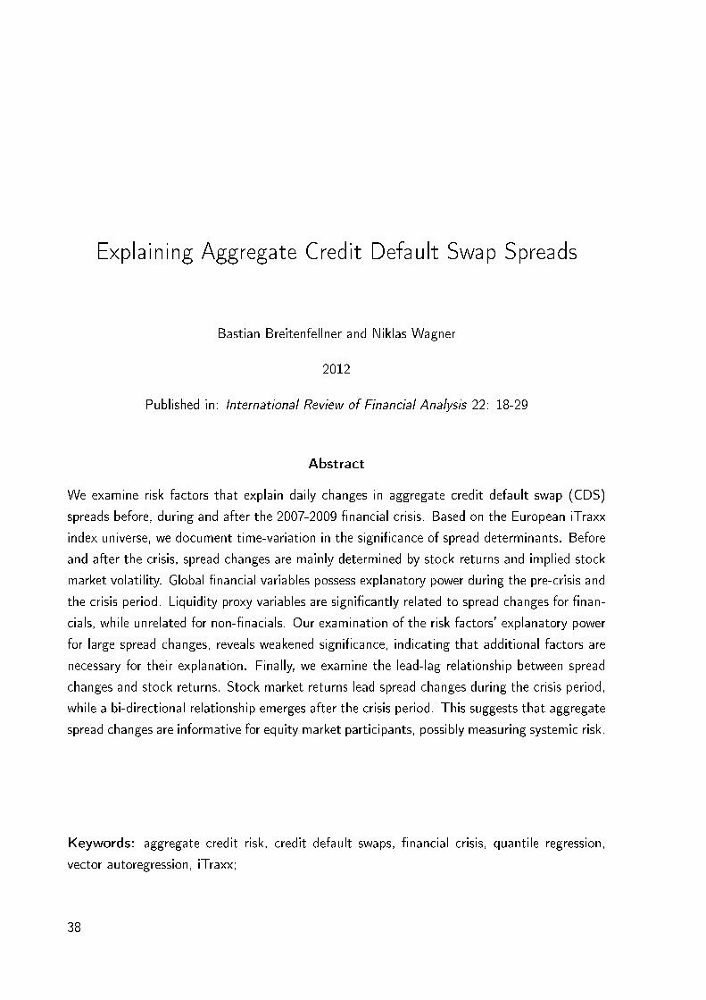
Explaining Aggregate Credit Default Swap Spreads
Bastian Breitenfellner and Niklas Wagner
2012
Published in: International Review of Financial Analysis 22: 18-29
Abstract
We examine risk factors that explain daily changes in aggregate credit default swap (CDS)
spreads before, during and after the 2007-2009 nancial crisis. Based on the European iTraxx
index universe, we document time-variation in the signicance of spread determinants. Before
and after the crisis, spread changes are mainly determined by stock returns and implied stock
market volatility. Global nancial variables possess explanatory power during the pre-crisis and
the crisis period. Liquidity proxy variables are signicantly related to spread changes for nan-
cials, while unrelated for non-nacials. Our examination of the risk factors' explanatory power
for large spread changes, reveals weakened signicance, indicating that additional factors are
necessary for their explanation. Finally, we examine the lead-lag relationship between spread
changes and stock returns. Stock market returns lead spread changes during the crisis period,
while a bi-directional relationship emerges after the crisis period. This suggests that aggregate
spread changes are informative for equity market participants, possibly measuring systemic risk.
Keywords: aggregate credit risk, credit default swaps, nancial crisis, quantile regression,
vector autoregression, iTraxx;
38
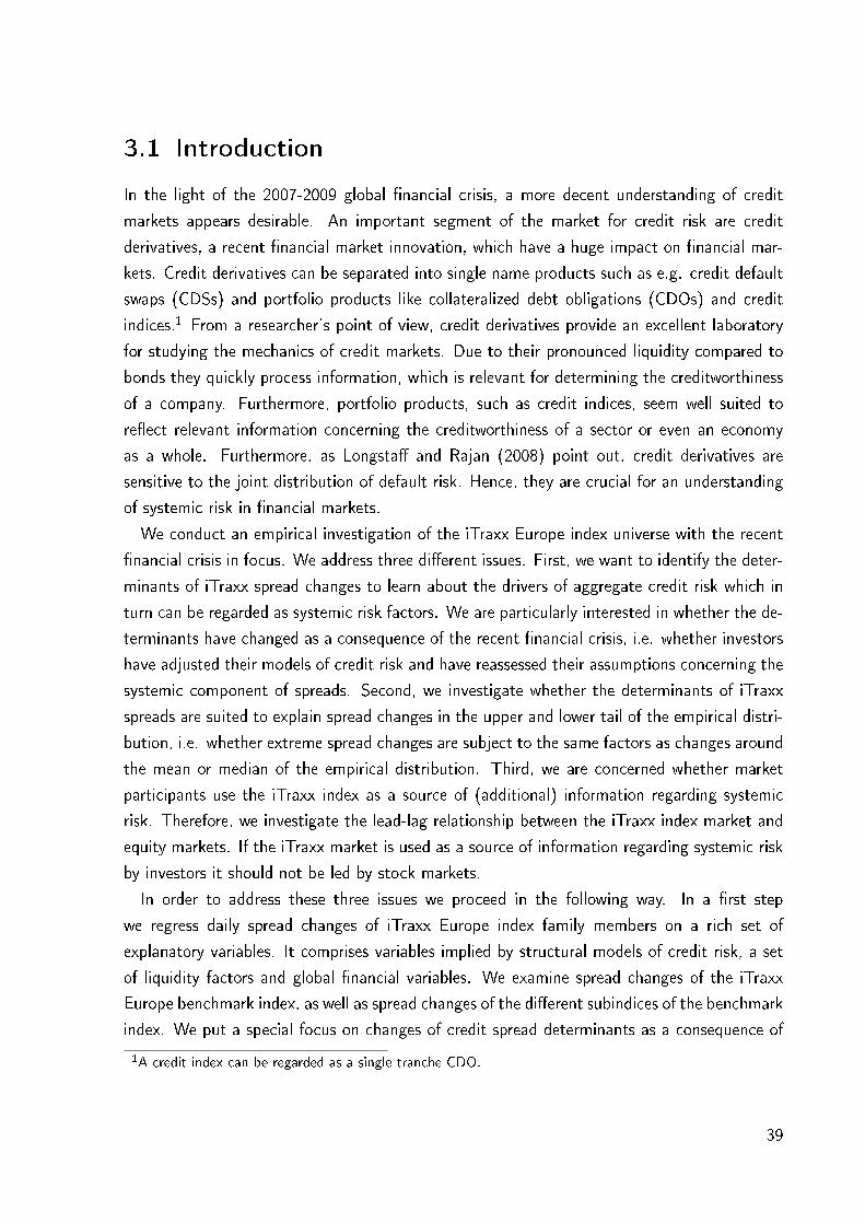
3.1 Introduction
In the light of the 2007-2009 global nancial crisis, a more decent understanding of credit
markets appears desirable. An important segment of the market for credit risk are credit
derivatives, a recent nancial market innovation, which have a huge impact on nancial mar-
kets. Credit derivatives can be separated into single name products such as e.g. credit default
swaps (CDSs) and portfolio products like collateralized debt obligations (CDOs) and credit
indices.1 From a researcher's point of view, credit derivatives provide an excellent laboratory
for studying the mechanics of credit markets. Due to their pronounced liquidity compared to
bonds they quickly process information, which is relevant for determining the creditworthiness
of a company. Furthermore, portfolio products, such as credit indices, seem well suited to
reect relevant information concerning the creditworthiness of a sector or even an economy
as a whole. Furthermore, as Longsta and Rajan (2008) point out, credit derivatives are
sensitive to the joint distribution of default risk. Hence, they are crucial for an understanding
of systemic risk in nancial markets.
We conduct an empirical investigation of the iTraxx Europe index universe with the recent
nancial crisis in focus. We address three dierent issues. First, we want to identify the deter-
minants of iTraxx spread changes to learn about the drivers of aggregate credit risk which in
turn can be regarded as systemic risk factors. We are particularly interested in whether the de-
terminants have changed as a consequence of the recent nancial crisis, i.e. whether investors
have adjusted their models of credit risk and have reassessed their assumptions concerning the
systemic component of spreads. Second, we investigate whether the determinants of iTraxx
spreads are suited to explain spread changes in the upper and lower tail of the empirical distri-
bution, i.e. whether extreme spread changes are subject to the same factors as changes around
the mean or median of the empirical distribution. Third, we are concerned whether market
participants use the iTraxx index as a source of (additional) information regarding systemic
risk. Therefore, we investigate the lead-lag relationship between the iTraxx index market and
equity markets. If the iTraxx market is used as a source of information regarding systemic risk
by investors it should not be led by stock markets.
In order to address these three issues we proceed in the following way. In a rst step
we regress daily spread changes of iTraxx Europe index family members on a rich set of
explanatory variables. It comprises variables implied by structural models of credit risk, a set
of liquidity factors and global nancial variables. We examine spread changes of the iTraxx
Europe benchmark index, as well as spread changes of the dierent subindices of the benchmark
index. We put a special focus on changes of credit spread determinants as a consequence of
1A credit index can be regarded as a single tranche CDO.
39

the recent nancial crisis. Our sample ranges from 06/16/2004 to 08/06/2010 and spans
the crisis period, as well as a pre- and a post-crisis period. This allows us to examine the
evolution of credit spread determinants throughout the nancial crisis. First we estimate our
econometric model for the full sample and then repeat the estimation for the pre-crisis, crisis
and post-crisis subsamples to detect changes in the set of spread drivers.
In a next step we reestimate our econometric model via quantile regression. This allows
us to examine the performance of our set of explanatory variables in the upper and lower
quantiles of the empirical distribution of spread changes, i.e. to check for the robustness of
our OLS-regression results in dierent quantile of the empirical distribution of spread changes.
The quantile regression is conducted for all subindices and all subsamples. This allows us
to study the determinants of spread changes in upper and lower quantiles of the empirical
distribution, as well as changes in the determinants in the course of the nancial crisis.
To examine whether market participants rely on the iTraxx index as a source of additional
information we examine the lead-lag relationship between the market for credit risk and stock
markets. For this purpose we estimate a vector autoregressive model with exogenous variables
(VARX-model). The exogenous variables are supposed to jointly determine credit spread
changes, as well as stock returns on a portfolio constructed out of the iTraxx index constituents.
We estimate the VARX-model for all subindices and all respective subsamples to investigate
whether the lead-lag relationship has been altered by the recent nancial crisis.
Our paper contributes to the existing literature in several ways. First we investigate the
explanatory power of a rich set of independent variables, including proxies for liquidity and
global nancial factors. Second, to the best of our knowledge, this is the rst empirical
investigation of the behavior of iTraxx index spreads of the benchmark index and all subindices
with a special focus on changes on credit spread determinants in the course of the recent
nancial crisis. Third, our empirical paper provides deeper insights into the mechanics of
iTraxx spreads by explicitly examining the behavior of credit spread changes at the upper and
lower quantiles of the empirical distribution. Finally, we contribute to the existing literature
by examining the evolution of lead-lag relationships between the iTraxx and stock returns in
the course of the recent nancial crisis, while controlling for several exogenous variables.
We nd strong evidence of variation in the determinants of credit spread changes in the
course of the recent nancial crisis. This nding suggests that market participants have altered
their models of credit risk as a consequence of the crisis. While the number of factors nec-
essary to explain iTraxx spread changes varies throughout the sample period, the explanatory
power of our set of independent variables rises. The predominant factor determining iTraxx
spread changes for all subsamples and all subindices is the return on an equal-weighted stock
40
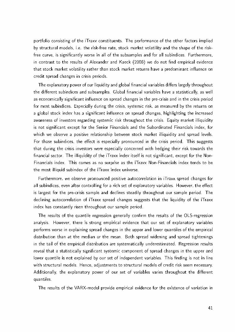
portfolio consisting of the iTraxx constituents. The performance of the other factors implied
by structural models, i.e. the risk-free rate, stock market volatility and the shape of the risk-
free curve, is signicantly worse in all of the subsamples and for all subindices. Furthermore,
in contrast to the results of Alexander and Kaeck (2008) we do not nd empirical evidence
that stock market volatility rather than stock market returns have a predominant inuence on
credit spread changes in crisis periods.
The explanatory power of our liquidity and global nancial variables diers largely throughout
the dierent subindices and subsamples. Global nancial variables have a statistically, as well
as economically signicant inuence on spread changes in the pre-crisis and in the crisis period
for most subindices. Especially during the crisis, systemic risk, as measured by the returns on
a global stock index has a signicant inuence on spread changes, highlighting the increased
awareness of investors regarding systemic risk throughout the crisis. Equity market illiquidity
is not signicant except for the Senior Financials and the Subordinated Financials index, for
which we observe a positive relationship between stock market illiquidity and spread levels.
For those subindices, the eect is especially pronounced in the crisis period. This suggests
that during the crisis investors were especially concerned with hedging their risk towards the
nancial sector. The illiquidity of the iTraxx index itself is not signicant, except for the Non-
Financials index. This comes as no surprise as the iTraxx Non-Financials index tends to be
the most illiquid subindex of the iTraxx index universe.
Furthermore, we observe pronounced positive autocorrelation in iTraxx spread changes for
all subindices, even after controlling for a rich set of explanatory variables. However, the eect
is largest for the pre-crisis sample and declines steadily throughout our sample period. The
declining autocorrelation of iTraxx spread changes suggests that the liquidity of the iTraxx
index has constantly risen throughout our sample period.
The results of the quantile regression generally conrm the results of the OLS-regression
analysis. However, there is strong empirical evidence that our set of explanatory variables
performs worse in explaining spread changes in the upper and lower quantiles of the empirical
distribution than at the median or the mean. Both spread widening and spread tightenings
in the tail of the empirical distribution are systematically underestimated. Regression results
reveal that a statistically signicant systemic component of spread changes in the upper and
lower quantile is not explained by our set of independent variables. This nding is not in line
with structural models. Hence, adjustments to structural models of credit risk seem necessary.
Additionally, the explanatory power of our set of variables varies throughout the dierent
quantiles.
The results of the VARX-model provide empirical evidence for the existence of variation in
41
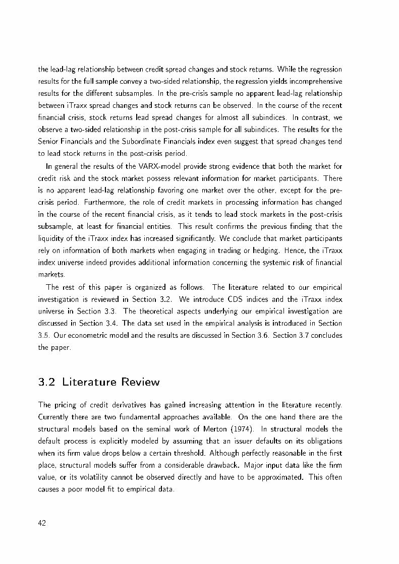
the lead-lag relationship between credit spread changes and stock returns. While the regression
results for the full sample convey a two-sided relationship, the regression yields incomprehensive
results for the dierent subsamples. In the pre-crisis sample no apparent lead-lag relationship
between iTraxx spread changes and stock returns can be observed. In the course of the recent
nancial crisis, stock returns lead spread changes for almost all subindices. In contrast, we
observe a two-sided relationship in the post-crisis sample for all subindices. The results for the
Senior Financials and the Subordinate Financials index even suggest that spread changes tend
to lead stock returns in the post-crisis period.
In general the results of the VARX-model provide strong evidence that both the market for
credit risk and the stock market possess relevant information for market participants. There
is no apparent lead-lag relationship favoring one market over the other, except for the pre-
crisis period. Furthermore, the role of credit markets in processing information has changed
in the course of the recent nancial crisis, as it tends to lead stock markets in the post-crisis
subsample, at least for nancial entities. This result conrms the previous nding that the
liquidity of the iTraxx index has increased signicantly. We conclude that market participants
rely on information of both markets when engaging in trading or hedging. Hence, the iTraxx
index universe indeed provides additional information concerning the systemic risk of nancial
markets.
The rest of this paper is organized as follows. The literature related to our empirical
investigation is reviewed in Section 3.2. We introduce CDS indices and the iTraxx index
universe in Section 3.3. The theoretical aspects underlying our empirical investigation are
discussed in Section 3.4. The data set used in the empirical analysis is introduced in Section
3.5. Our econometric model and the results are discussed in Section 3.6. Section 3.7 concludes
the paper.
3.2 Literature Review
The pricing of credit derivatives has gained increasing attention in the literature recently.
Currently there are two fundamental approaches available. On the one hand there are the
structural models based on the seminal work of Merton (1974). In structural models the
default process is explicitly modeled by assuming that an issuer defaults on its obligations
when its rm value drops below a certain threshold. Although perfectly reasonable in the rst
place, structural models suer from a considerable drawback. Major input data like the rm
value, or its volatility cannot be observed directly and have to be approximated. This often
causes a poor model t to empirical data.
42
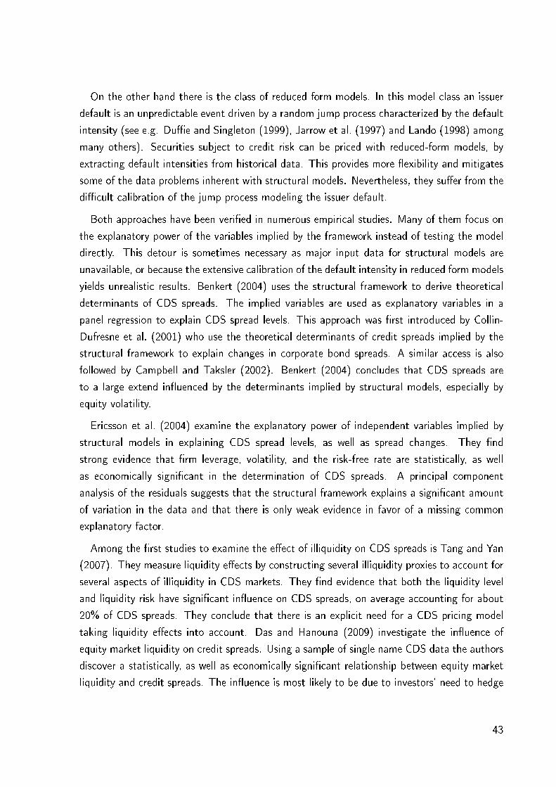
On the other hand there is the class of reduced form models. In this model class an issuer
default is an unpredictable event driven by a random jump process characterized by the default
intensity (see e.g. Due and Singleton (1999), Jarrow et al. (1997) and Lando (1998) among
many others). Securities subject to credit risk can be priced with reduced-form models, by
extracting default intensities from historical data. This provides more exibility and mitigates
some of the data problems inherent with structural models. Nevertheless, they suer from the
dicult calibration of the jump process modeling the issuer default.
Both approaches have been veried in numerous empirical studies. Many of them focus on
the explanatory power of the variables implied by the framework instead of testing the model
directly. This detour is sometimes necessary as major input data for structural models are
unavailable, or because the extensive calibration of the default intensity in reduced form models
yields unrealistic results. Benkert (2004) uses the structural framework to derive theoretical
determinants of CDS spreads. The implied variables are used as explanatory variables in a
panel regression to explain CDS spread levels. This approach was rst introduced by Collin-
Dufresne et al. (2001) who use the theoretical determinants of credit spreads implied by the
structural framework to explain changes in corporate bond spreads. A similar access is also
followed by Campbell and Taksler (2002). Benkert (2004) concludes that CDS spreads are
to a large extend inuenced by the determinants implied by structural models, especially by
equity volatility.
Ericsson et al. (2004) examine the explanatory power of independent variables implied by
structural models in explaining CDS spread levels, as well as spread changes. They nd
strong evidence that rm leverage, volatility, and the risk-free rate are statistically, as well
as economically signicant in the determination of CDS spreads. A principal component
analysis of the residuals suggests that the structural framework explains a signicant amount
of variation in the data and that there is only weak evidence in favor of a missing common
explanatory factor.
Among the rst studies to examine the eect of illiquidity on CDS spreads is Tang and Yan
(2007). They measure liquidity eects by constructing several illiquidity proxies to account for
several aspects of illiquidity in CDS markets. They nd evidence that both the liquidity level
and liquidity risk have signicant inuence on CDS spreads, on average accounting for about
20% of CDS spreads. They conclude that there is an explicit need for a CDS pricing model
taking liquidity eects into account. Das and Hanouna (2009) investigate the inuence of
equity market liquidity on credit spreads. Using a sample of single name CDS data the authors
discover a statistically, as well as economically signicant relationship between equity market
liquidity and credit spreads. The inuence is most likely to be due to investors' need to hedge
43
their credit exposure in equity markets.
While the aforementioned studies focus on single name credit risk, there is a growing amount
of literature covering portfolio products such as CDS indices. In one of the rst empirical
papers with a focus on credit indices Byström (2005) analyzes the relationship between equity
market returns, equity market volatility and iTraxx spreads. He nds strong evidence that
current, as well as lagged stock returns explain much of the variation in CDS index spreads.
Furthermore he discovers signicant correlations between stock markets and CDS markets,
whereas the stock market seems to lead the CDS market in the transmission of rm specic
information. Alexander and Kaeck (2008) introduce a Markov switching model to examine
the determinants of iTraxx Europe index spreads in two dierent regimes. They conrm the
statistically signicant explanatory power of the variables implied by the structural framework.
Additionally, they nd that CDS spreads are more sensitive to stock returns than stock volatility
in normal market conditions. In times of turbulences, spreads are extremely sensitive to stock
volatility. Scheicher (2008) analyzes to what extent the set of explanatory variables governing
iTraxx CDX tranche spreads has changed during the recent global nancial crisis. The author
nds empirical evidence that a decreasing risk appetite of investors, as well as concerns about
market liquidity have contributed to the rising spread levels during the crisis. Furthermore,
the author discovers that the repricing of tranches during the crisis is more pronounced in
the CDX than in the iTraxx index universe. Giammarino and Barrieu (2009) use an adaptive
nonparametric modeling approach to explain iTraxx spreads by tradeable market factors. Their
model allows for dynamic factor sensitivities. The authors nd empirical evidence for signicant
variation in factor sensitivities. During crises, factor sensitivities may be subject to sudden
jumps while showing pronounced time consistency in calm periods.
Lead-lag relationships between the market for credit risk and stock markets have been
addressed in several empirical studies. For example Norden and Weber (2009) analyze the
relationship between CDS, bond and stock markets with a vector autoregressive model. The
authors nd empirical evidence that stock markets lead CDS and bond markets, while CDS
spread changes lead bond spread changes. The co-movement between CDS spreads and bond
returns is especially pronounced for companies with low credit quality or large bond issues.
Fung et al. (2008) examine the relationship between the U.S. stock market and the CDS
markets. The authors discover that the stock market leads the CDS index market in price
discovery. However, CDS markets have a crucial role in the volatility spillover between the
two markets. The authors conclude that both markets provide relevant information for market
participants.
44
3.3 Characteristics of CDS Contracts and CDS Indices
A CDS can be regarded as an insurance against the default of a certain issuer of debt capital,
called reference entity, at the cost of a periodic fee, called spread. In case of an issuer default,
the protection buyer is compensated for his losses due to the default by the protection seller.
Therefore, CDS spreads can be regarded as a measure for the credit risk of the reference
entity, as they represent the compensation an investor has to be oered in order to be willing
to obtain exposure to the reference entity's default risk. In contrast to a classical insurance
contract, an engagement in a CDS contract does not require owning the reference asset.
Credit indices are among the major nancial innovations in the new millennium. In contrast
to single name CDSs they allow to insure a whole portfolio of single name credit risk with a
single transaction. The outcome is similar to buying protection on each of the names in the
portfolio. Hence credit indices can be regarded as an aggregation of single name CDSs.
3.3.1 The iTraxx Europe Index Family
Up to date there exist two major families of credit indices, the Dow Jones CDX index universe,
covering North America and emerging markets, and the iTraxx index universe, with a regional
focus on Europe and Asia. The iTraxx Europe benchmark index consists of 125 European
entities with an investment grade rating (Markit (2011)). Among the subindices of the iTraxx
Europe benchmark index are the iTraxx HighVol, the iTraxx Senior Financials, the iTraxx
Subordinated Financials and the iTraxx Non-Financials index.2 The iTraxx Senior and Subor-
dinated Financial indices comprise the same set of constituents, while oering protection on
dierent (senior vs. subordinated) reference obligations. Within each index, the constituents
are weighted equally. The indices are rolled twice a year. At each role date the constituents
of the respective index are determined according to a liquidity poll, ranking entities based on
the trading volume in the CDS market in the previous six months.3 The sectoral breakdown
of the nal 125 index constituents is as follows:
• 30 Autos & industrials,
• 30 Consumers,
• 20 Energy,
2The iTraxx index family was formed as a result of the merger of the iBoxx and Trac-X indices in June 2004.Each iTraxx index family consists of a benchmark index and further subindices. There had been furthersectoral indices in the past, which are no longer rolled.
3For further details regarding the membership determination details refer to Markit (2011).
45

• 20 TMT (Technology, Media and Telecommunication),
• 25 Financials.
In case one of the index constituents is subject to a credit event, the entity is removed from
the index. The notional of the index is reduced accordingly. The credit event triggers a payout
from the protection seller to the protection buyer. The settlement can either be physical or in
cash.
3.3.2 Index Pricing
Markit calculates both quoted and theoretical index prices and levels. The procedures are
described in Markit (2010b). Quoted index prices and spreads are calculated as the arithmetic
average of prices and spreads quoted by market makers. The calculated spread has to be
based on quotes of at least three dierent market makers. The highest an the lowest quotes
are discarded and do not enter the calculation in order to eliminate outliers.
In addition to the quoted spreads, theoretical spreads are calculated as a benchmark of the
pricing accuracy of market participants. The calculation is based on spread data for each of the
index constituents. The spread data is used to construct a spread curve for each constituent.
Spreads for terms which are not traded are obtained via linear interpolation. The spread
curves are used to calculate the survival probabilities at each coupon payment date for each
index constituent. Then the present value (PV) and the accrued interest (AI) for each index
constituent is calculated.4 These are aggregated to the index PV (PV ) and accrued interest
(AI) by calculating the weighted averages of the constituents's PVs and accrued interest. The
index price is then calculated as
Pindex = 1 + PV − AI. (3.1)
The theoretical index spread is obtained by solving for the at curve that gives PV .
3.4 Background
3.4.1 Spread Modeling
The theoretical framework we rely on for our empirical analysis is based on the ndings of Lando
(1998) and the reduced form pricing framework of Due and Singleton (1999). Reduced form
4An example of how the PV of an constituent is calculated is give in Markit (2010a).
46
models treat default as an unpredictable event driven by a hazard process λt. The mean loss
rate at time t is given by λtLt, where Lt is the expected fractional loss of market value in
case of a default at time t. Given that the mean loss rate process λtLt is exogenous, standard
term structure models are applicable to the pricing of default risky claims, by parameterizing
the risk-adjusted short rate process Rt = rt + λtLt instead of the short rate process rt (see
Lando (1998)).
This nding is used by Due and Singleton (1999) to price contingent claims subject to
credit risk as follows. Suppose an arbitrage-free setting where all claims are priced under the
equivalent martingale measure Q. Next, suppose that a contingent claim is a pair (Z, τ),
where Z is a random variable representing a payment and τ is the time when Z is paid. The
price process V of a given contingent claim (Z, τ) is given by
Vt = EQt
exp
− τ∫t
Rt dt
Z
, t < τ, (3.2)
where EQt represents the risk neutral, conditional expectation at date t given the information
ltration F .Some empirical studies like Berndt et al. (2005) and Pan and Singleton (2005) observe
actual CDS spreads which are systematically higher than those implied by reduced-form pricing
models. In the arbitrage-free setting of this framework we would expect these mispricings to
be fully arbitraged away, which is obviously not the case. A possible explanation for this puzzle
are frictions due to illiquidity eects, which in turn hamper arbitrage.
In order to account for illiquidity eects in the reduced-form pricing framework for contingent
claims subject to credit risk, Due and Singleton (2003) propose that an liquidity premium
should directly be applied in terms of a price discount for the valuation of contingent claims,
such as CDS. Therefore, the risk-adjusted short-rate process is expressed as
Rt = rt + λtLt + `t, (3.3)
where `t represents an liquidity premium, which can be interpreted as the risk-neutral expected
fractional loss due to illiquidity eects.
3.4.2 Implications for our Empirical Investigation
As outlined in the previous section, specifying the risk-adjusted short rate process Rt is essential
for pricing claims subject to credit risk, such as bonds and CDS. Given that a credit index
47

has to be priced, the claim is contingent on the solvency of a portfolio of obligors. Hence,
Rt has to reect the risk of the portfolio of index constituents. Nevertheless, as the index
PV is calculated as the weighted average of the constituents's PVs, there is no fundamental
dierence between the pricing of the iTraxx index and a e.g. a single name CDS. In the
remainder we are concerned with identifying the determinants of Rt. The variables implied
by structural models of credit risk are natural candidates. However, since Rt cannot be fully
explained by these variables, additional factors determining Rt, such as illiquidity components
have to be incorporated.
3.5 Data
In this section we introduce the data set used for our empirical analysis. The iTraxx data is
described in Section 3.5.1 and the independent variables used are introduced in Section 3.5.2.
3.5.1 iTraxx Spread Data
Our dataset consists of daily bid and ask quotes of the rst 13 series of the iTraxx Europe
benchmark index, as well as the subindices of the iTraxx Europe universe. We chose a tenor
of ve years as this is the most liquid maturity available. The sample ranges from June 16th
2004 to August 6th 2010 and comprises 1603 trading days. The sample is also split into three
subsamples. Sample lengths are chosen according to the results of a Chow-breakpoint test with
5% signicance level. Rather than analyzing every roll of the index on its own, we aggregate
the single iTraxx series to form a single time series of iTraxx spreads for each (sub)index.
This may lead to distortions, i.e. jumps in the index levels, as the index constituents change
with every roll. However, the number of changes is moderate, thus there are no large spread
dierences between the single roll dates. The current index mid-spread is calculated as the
arithmetic mean of the bid and ask quotes. The data set is obtained from Open Bloomberg.
We analyze daily spread changes in order to have sucient observations to obtain robust
results, despite the large amount of independent variables and the fact that the sample is
divided into subsamples. In the empirical analysis we focus on spread changes rather than on
spread levels, since spread levels are non-stationary, as conrmed by a unit root test. A time
series plot for both iTraxx spread levels and spread changes is shown in Figure 3.1.
The upper panel of Figure 3.1 illustrates the massive impact of the global nancial crisis on
the iTraxx Europe benchmark index. Since the rst series of the iTraxx Europe index the mid-
spread had declined steadily, besides a peak at May 2005 at about 60 basis points (bps) when
Ford and general Motors were downgraded, from about 45 bps in June 2004 to the all-time
48
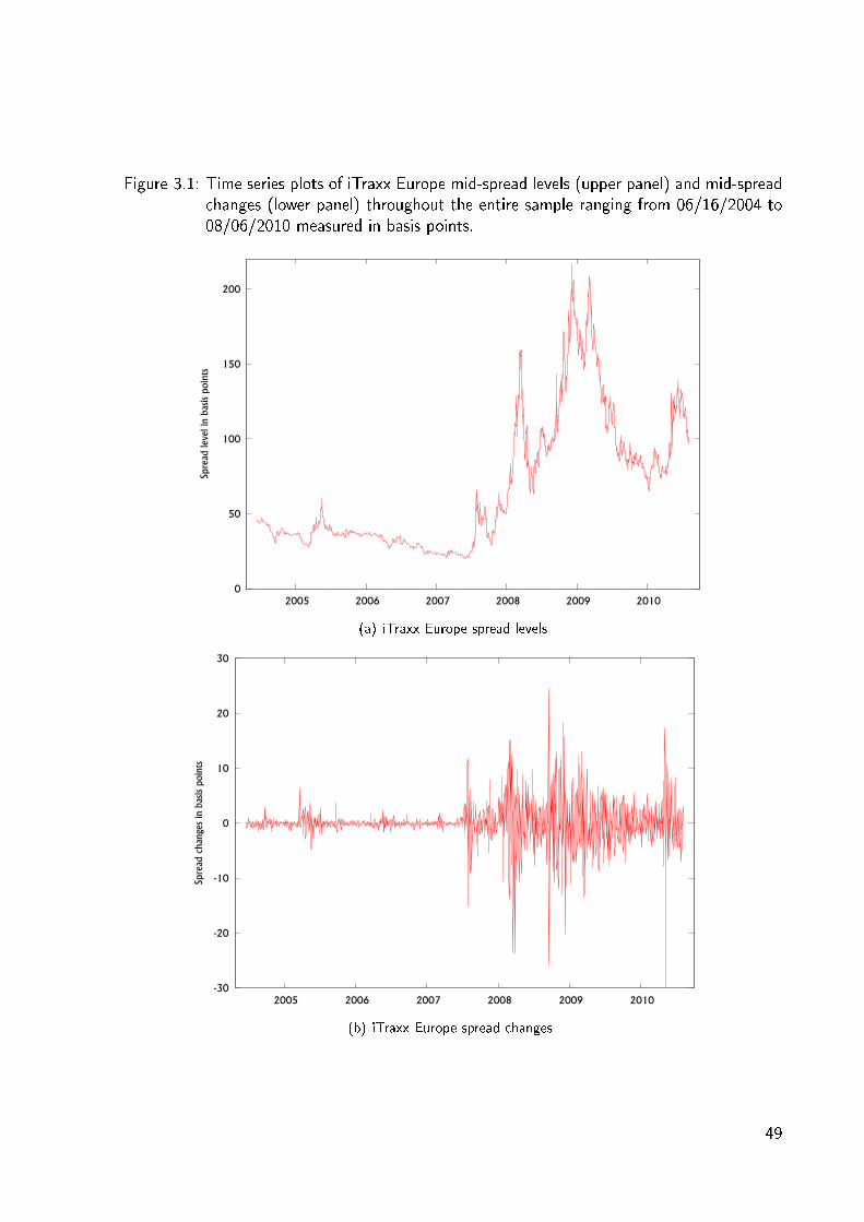
Figure 3.1: Time series plots of iTraxx Europe mid-spread levels (upper panel) and mid-spreadchanges (lower panel) throughout the entire sample ranging from 06/16/2004 to08/06/2010 measured in basis points.
0
50
100
150
200
2005 2006 2007 2008 2009 2010
Spre
ad le
vel i
n ba
sis p
oint
s
(a) iTraxx Europe spread levels
-30
-20
-10
0
10
20
30
2005 2006 2007 2008 2009 2010
Spre
ad c
hang
es in
bas
is po
ints
(b) iTraxx Europe spread changes
49
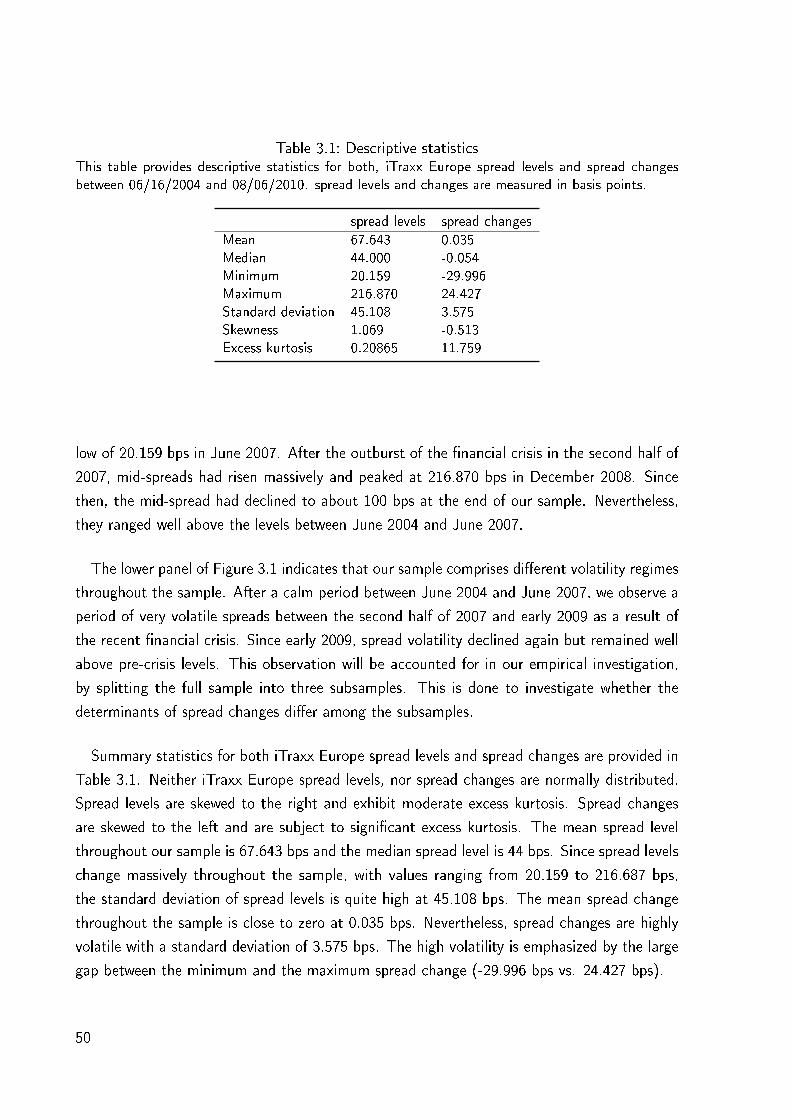
Table 3.1: Descriptive statisticsThis table provides descriptive statistics for both, iTraxx Europe spread levels and spread changesbetween 06/16/2004 and 08/06/2010. spread levels and changes are measured in basis points.
spread levels spread changes
Mean 67.643 0.035Median 44.000 -0.054Minimum 20.159 -29.996Maximum 216.870 24.427Standard deviation 45.108 3.575Skewness 1.069 -0.513Excess kurtosis 0.20865 11.759
low of 20.159 bps in June 2007. After the outburst of the nancial crisis in the second half of
2007, mid-spreads had risen massively and peaked at 216.870 bps in December 2008. Since
then, the mid-spread had declined to about 100 bps at the end of our sample. Nevertheless,
they ranged well above the levels between June 2004 and June 2007.
The lower panel of Figure 3.1 indicates that our sample comprises dierent volatility regimes
throughout the sample. After a calm period between June 2004 and June 2007, we observe a
period of very volatile spreads between the second half of 2007 and early 2009 as a result of
the recent nancial crisis. Since early 2009, spread volatility declined again but remained well
above pre-crisis levels. This observation will be accounted for in our empirical investigation,
by splitting the full sample into three subsamples. This is done to investigate whether the
determinants of spread changes dier among the subsamples.
Summary statistics for both iTraxx Europe spread levels and spread changes are provided in
Table 3.1. Neither iTraxx Europe spread levels, nor spread changes are normally distributed.
Spread levels are skewed to the right and exhibit moderate excess kurtosis. Spread changes
are skewed to the left and are subject to signicant excess kurtosis. The mean spread level
throughout our sample is 67.643 bps and the median spread level is 44 bps. Since spread levels
change massively throughout the sample, with values ranging from 20.159 to 216.687 bps,
the standard deviation of spread levels is quite high at 45.108 bps. The mean spread change
throughout the sample is close to zero at 0.035 bps. Nevertheless, spread changes are highly
volatile with a standard deviation of 3.575 bps. The high volatility is emphasized by the large
gap between the minimum and the maximum spread change (-29.996 bps vs. 24.427 bps).
50

3.5.2 Independent Variables
The set of independent variables used is based on the theoretical methodology outlined in
Section 3.4. Natural candidates to use for the regression analysis are the variables implied by
structural models. Unfortunately not all factors implied by structural models are observable
and therefore have to be proxied by observable factors. Furthermore, additional variables seem
necessary, as variables implied by structural models fail to capture all the variation in credit
spreads. Hence, we augment the set of variables used with liquidity, as well as global nan-
cial variables. In the remainder of this section we introduce the independent variables used
for the empirical analysis and explain their theoretical inuence on iTraxx Europe spread levels.
Variables implied by structural models
Structural models are appealing when it comes to explain the mechanics behind the default
process of a company. Since the factors implied by structural models have a theoretical
underpinning, it is straightforward to include them in an empirical investigation on spread
determinants. The variables included in our econometric models are discussed below.
The risk-free rate
According to structural models the eects of the risk-free rate are twofold. On the one hand,
an increasing risk-free rate leads to an increasing drift rate of the company value. The higher
the drift rate, the more likely the company value is to remain above the default boundary
and thus default risk decreases. On the other hand, a higher risk-free rate refers to a higher
discount rate, which decreases the present value of future cash ows. This eect devalues the
put option of the company's owners. Both eects imply that a rising risk-free rate should lead
to a decrease in credit spreads. In the empirical analysis we use the one year Euribor rate as
a proxy for the risk-free rate.
The company value
Another important factor in structural models is the company value. An increasing company
value raises the distance-to-default of the respective entity. The distance-to-default measures
the number of standard deviations the rm value lies above the default barrier. The higher the
distance-to-default the more unlikely the entity is to hit the barrier, i.e. the lower the credit
risk. Thus, an increasing company value theoretically leads to lower credit spreads. As the
company value is not directly observable and we investigate spread changes rather than spread
levels, we refer to stock returns as a proxy for changes in the company value.
51

To examine the eect of stock returns on iTraxx Europe spread changes we form equal
weighted stock portfolios for every iTraxx series. The portfolio constituents comprise the
constituents of the respective iTraxx series. If an iTraxx constituent has no traded stock or
no stock data is available for the respective entity it is removed from the portfolio and the
portfolio weights are adjusted accordingly. If the iTraxx constituent has no traded equity but
is a subsidiary of a parent with traded equity, the parent is included into the portfolio. All
equity prices are converted to Euro currency to avoid biases due to exchange rate eects. We
calculate the log-return of the portfolios on a daily basis and aggregate the portfolio returns
to a single time series to match the iTraxx time series. The equity data set is obtained from
Thomson One Banker.
The volatility of the company value
Since structural models of credit risk rely on option pricing arguments, the volatility of the
company value is another important driver of credit spreads. The higher the volatility the more
valuable is the put option of the company owners and the less valuable is the value of the
rms debt. Therefore, rising equity volatility leads to an increase of the respective company's
spreads.
As the volatility of the company value is not directly observable stock volatility is used as a
proxy. Therefore we calculate the standard deviation of the equity portfolios described above
using a rolling window containing the preceding 20 return observations. The volatilities then
are aggregated to a time series matching the iTraxx Europe time series.
The slope of the risk-free term structure
When the risk-free rate is assumed to be time-varying, an increasing slope of the yield curve
implies a higher spot rate in the future. This is because an increasing slope causes forward
rates to increase, which are similar to expected future spot rates. Hence, an increasing slope
of the risk-free curve should lower credit spreads. We calculate the slope of the risk-free curve
as the dierence between the one year Euribor and the Eonia overnight rate.
Liquidity variables
In the empirical analysis we account for two possible sources of illiquidity eects. On the
one hand illiquidity in the iTraxx Europe index itself could have a signicant inuence on the
spreads. On the other hand equity market illiquidity is another possible factor priced.
52

Liquidity in the market for credit risk
We use the quoted bid-ask spread changes of the iTraxx Europe index as a proxy for illiquidity
in the market for credit risk. Bid-ask spreads are widely used as liquidity proxies in empirical
studies. Wider bid-ask spreads are a sign for growing illiquidity in the market. This in turn
may be interpreted as a sign of growing market uncertainty and therefore rising risks in the
market, which causes spreads to widen. Additionally, if investors demand a risk premium for
illiquidity, the factor should be priced in iTraxx spreads and growing illiquidity should cause
spreads to widen. Bid and ask quotes for the iTraxx Europe index are obtained from Open
Bloomberg. The spread is calculated as the dierence between the quoted bid and ask spread
of the respective index.
Equity market illiquidity
Equity market illiquidity is another factor, which is believed to be priced in credit spreads. Das
and Hanouna (2009) argue that equity market liquidity is priced in the market for credit risk
due to hedging activities. If investors hedge their positions in the market for credit risk via
equity markets, growing illiquidity causes hedges to be more expensive. This in turn will cause
spreads to rise. Unfortunately, equity market liquidity, especially on a market or portfolio level,
is not directly observable and dicult to proxy. To date several methods to measure market
liquidity have been proposed. We employ the liquidity measure of Amihud (2002)
The measure of Amihud (2002) is based on the idea that in a perfectly liquid market, large
trades should have no impact on prices as long as the trade is not induced by price relevant
information. Therefore, equity market liquidity is expressed by the AILLIQ-measure, which
relates price changes to trading volume. It is calculated as
AILLIQt =1
Nt
Nt∑t=1
|Ri,t|V OLDi,t
, (3.4)
where Nt is the number of stocks at time t, Ri,t is the time t return of stock i, and V OLDi,t
is the daily trading volume in Euro currency (EUR) of stock i at time t.5 Since the AILLIQ-
measure typically yields very small values, we multiply it by 106 to make it more manageable
for our regression analysis.
Global nancial variables
5Note that we do not take a time average of the ratio|Ri,t|
V OLDi,tas it is done by Amihud (2002) to dampen
the eect of outliers. In our case this is achieved by taking the average over our stock portfolio.
53

We include several global nancial variables, which account for macroeconomic eects into
the econometric model. The recent nancial crisis has shown that credit spreads do not seem
to be solely driven by rm-specic data.
The state of the global economy
As a consequence of the globalization the state of the world economy is of rising importance
for companies. A global recession will result in growing default rates around the world and
will lead to higher credit spreads. To proxy for the state of the world economy we include the
MSCI World log index returns as an explanatory variable in our econometric model. The data
is obtained from Thomson One Banker.
Global market risk
Rising perceptions of global market risk, measured by implied stock market volatility, can be
regarded as a sign of growing uncertainty in nancial markets. This in turn will lead to higher
spreads in credit markets, as defaults are more likely in times of market stress. We include the
VStoxx implied volatility index as a measure of market risk. Besides measuring market risk,
the VStoxx index has additional appeal for our empirical analysis, as it can be regarded as a
proxy for the implied volatility of iTraxx constituents. Although we calculate the volatility of
the equity portfolio including the members of the iTraxx index, this measure might not capture
the perceptions of future volatility, which is the case for the VStoxx index.
Crisis indicator
In times of market distress many investors seek to curtail their risk exposure and invest in safe
assets. A classical, so called save harbor, is gold. Therefore we include gold price changes as
a proxy for changes in the risk appetite of investors and the stability of nancial markets. In
times of distress, the risk appetite of investors and the stability of the market declines and
investments such as gold become more popular, leading to rising gold prices. In times of
crisis, defaults are more likely, so rising gold prices should lead to rising iTraxx spread levels.
We employ daily gold price quotes from the London afternoon xing and calculate daily log-
returns of the gold price. The data is download from the website of Deutsche Bundesbank
(www.buba.de).
54

Table 3.2: Independent variables included in the econometric modelThe table contains the explanatory variables used in the empirical analysis as well as the signsof regression coecients as predicted by theory.
Explanatory Variable Description Predicted Sign∆Euribor Change in the Euribor rate -RP Return on the stock portfolio comprising iTraxx in-
dex constituents-
∆V olP Change of the trailing volatility of the stock port-folio comprising iTraxx index constituents
+
∆Steep Change in the steepness of the risk-free curve -∆Spread Change of the bid-ask spread of the iTraxx index +∆AILLIQ Change in the Amihud-Liquidity measure for the
stock portfolio comprising iTraxx index constituents+
RMSCI Return on the MSCI World index -∆V Stoxx Change in the VStoxx volatility index +RGold Return on the gold price +∆iT raxxt−1 Lagged change of the iTraxx spread +/-
Summary
Table 3.2 gives an overview of all variables included in the econometric model and signs of the
regression coecients predicted by theory.
3.6 Empirical Analysis
Our empirical analysis seeks to nd answers to ve research questions:
• What are the determinants of aggregate credit spread cahnges and consequently systemic
risk?
• How do the determinants evolve throughout the recent nancial crisis?
• Do the determinants dier for the single subindices?
• Do the determinants of aggregate credit spread changes dier within the various quantiles
of the empirical distribution?
• Do market participants use information provided by aggregate credit spreads as a measure
of systemic risk?
55
For this purpose we conduct our empirical analysis in the following way. First we examine
the determinants of iTraxx spread changes and their evolution throughout the recent nancial
crisis by estimating an OLS-regression model. We analyze the iTraxx Europe benchmark index,
as well as all of its subindices. Our goal is to achieve a better understanding of the drivers of
systemic risk in nancial markets and their underlying dynamics. The results are presented in
Section 3.6.1. In oder to check for the robustness of the OLS-regression results and to examine
the performance of our set of independent variables in the upper and lower quantiles of the
empirical distribution of spread changes, we additionally provide results for a quantile regression
in Section 3.6.2. Finally, we investigate the lead-lag relationship between the market for credit
risk and the stock market by estimating a VARX-model to assess whether the systematic
risk component contained in iTraxx spreads is actually priced by market participants. If it is,
iTraxx spread changes should not be led by stock returns. The results for the VARX-model
are discussed in Section 3.6.3.
Using daily spread changes leaves us with sucient observations under a division of our
sample into subsamples. We split the sample into three subsamples based on the results of
a Chow (1960) breakpoint test. Our analysis reveals that the null hypothesis of no structural
break at a given date can be rejected at the 5 percent signicance level and with a p-Value of
0.000 for July 2, 2007. The same holds for May 1, 2009 with a p-Value of 0.035. Given these
results and the historical setting as outlined in Section 3.5.1, we label the rst subsample as
"pre-crisis" (June 16, 2004 to July 2, 2007), the second subsample as "crisis" (July 3, 2007
to May 1, 2009) and the nal subsample as "post-crisis" (May 2, 2009 to August 6, 2010)
period.
3.6.1 OLS-Regression Results
In this section we investigate the determinants of iTraxx spread changes. We check for the
explanatory power of a large set of independent variables. Additionally, we investigate the
evolution of spread determinants throughout the recent nancial crisis. We perform the in-
vestigation for the whole sample period, as well as for three subsamples. These comprise
a pre-crisis sample a crisis sample and a post-crisis sample. The sample lengths are chosen
according to a Chow-breakpoint test with a signicance level of 5%. We repeat the anylsis for
the benchmark index, as well as all subindices of the iTraxx index family. For this purpose we
56
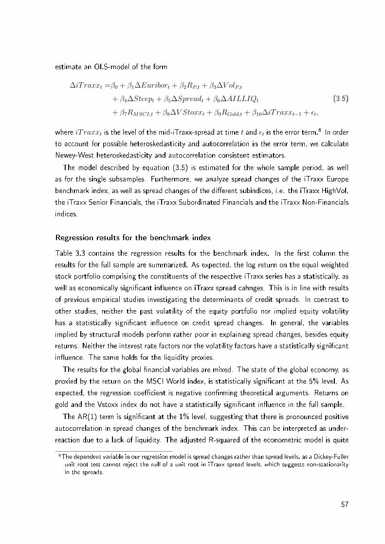
estimate an OLS-model of the form
∆iT raxxt =β0 + β1∆Euribort + β2RP,t + β3∆V olP,t
+ β4∆Steept + β5∆Spreadt + β6∆AILLIQt
+ β7RMSCI,t + β8∆V Stoxxt + β9RGold,t + β10∆iT raxxt−1 + εt,
(3.5)
where iT raxxt is the level of the mid-iTraxx-spread at time t and εt is the error term.6 In order
to account for possible heteroskedasticity and autocorrelation in the error term, we calculate
Newey-West heteroskedasticity and autocorrelation consistent estimators.
The model described by equation (3.5) is estimated for the whole sample period, as well
as for the single subsamples. Furthermore, we analyze spread changes of the iTraxx Europe
benchmark index, as well as spread changes of the dierent subindices, i.e. the iTraxx HighVol,
the iTraxx Senior Financials, the iTraxx Subordinated Financials and the iTraxx Non-Financials
indices.
Regression results for the benchmark index
Table 3.3 contains the regression results for the benchmark index. In the rst column the
results for the full sample are summarized. As expected, the log return on the equal weighted
stock portfolio comprising the constituents of the respective iTraxx series has a statistically, as
well as economically signicant inuence on iTraxx spread cahnges. This is in line with results
of previous empirical studies investigating the determinants of credit spreads. In contrast to
other studies, neither the past volatility of the equity portfolio nor implied equity volatility
has a statistically signicant inuence on credit spread changes. In general, the variables
implied by structural models perform rather poor in explaining spread changes, besides equity
returns. Neither the interest rate factors nor the volatility factors have a statistically signicant
inuence. The same holds for the liquidity proxies.
The results for the global nancial variables are mixed. The state of the global economy, as
proxied by the return on the MSCI World index, is statistically signicant at the 5% level. As
expected, the regression coecient is negative conrming theoretical arguments. Returns on
gold and the Vstoxx index do not have a statistically signicant inuence in the full sample.
The AR(1) term is signicant at the 1% level, suggesting that there is pronounced positive
autocorrelation in spread changes of the benchmark index. This can be interpreted as under-
reaction due to a lack of liquidity. The adjusted R-squared of the econometric model is quite
6The dependent variable in our regression model is spread changes rather than spread levels, as a Dickey-Fullerunit root test cannot reject the null of a unit root in iTraxx spread levels, which suggests non-stationarityin the spreads.
57
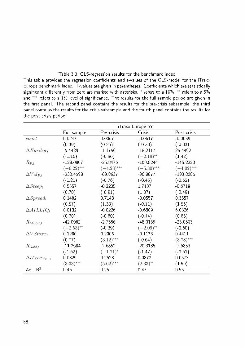
Table 3.3: OLS-regression results for the benchmark indexThis table provides the regression coecients and t-values of the OLS-model for the iTraxxEurope benchmark index. T-values are given in parentheses. Coecients which are statisticallysignicant dierently from zero are marked with asterisks. ∗ refers to a 10%, ∗∗ refers to a 5%and ∗∗∗ refers to a 1% level of signicance. The results for the full sample period are given inthe rst panel. The second panel contains the results for the pre-crisis subsample, the thirdpanel contains the results for the crisis subsample and the fourth panel contains the results forthe post-crisis period.
iTraxx Europe 5YFull sample Pre-crisis Crisis Post-crisis
const 0.0247 0.0067 -0.0617 -0.0039(0.39) (0.26) (-0.30) (-0.03)
∆Euribort -5.4489 -1.1756 -18.2117 25.4492(-1.16) (-0.96) (−2.19)∗∗ (1.42)
RP,t -128.0807 -25.8476 -160.8244 -145.2223(−6.22)∗∗∗ (−4.23)∗∗∗ (−5.30)∗∗∗ (−4.02)∗∗∗
∆V olP,t -230.4598 -69.8637 -96.8877 -193.8085(-1.21) (-0.76) (-0.45) (-0.62)
∆Steept 0.5357 -0.2205 1.7187 -0.6719(0.70) (-0.91) (1.07) (-0.49)
∆Spreadt 0.1482 0.7148 -0.0557 0.3557(0.57) (1.33) (-0.11) (1.56)
∆AILLIQt 0.0132 -0.0226 -0.6809 6.0326(0.20) (-0.80) (-0.14) (0.83)
RMSCI,t -42.0082 -2.7386 -48.0169 -23.0503(−2.53)∗∗ (-0.39) (−2.09)∗∗ (-0.60)
∆V Stoxxt 0.1280 0.2005 -0.1178 0.4411(0.77) (3.12)∗∗∗ (-0.64) (3.78)∗∗∗
RGold,t -11.2684 -2.6852 -20.3185 -7.6853(-1.62) (−1.71)∗ (-1.47) (-0.61)
∆iT raxxt−1 0.0829 0.2528 0.0872 0.0573(3.33)∗∗∗ (5.62)∗∗∗ (2.33)∗∗ (1.50)
Adj. R2 0.46 0.25 0.47 0.55
58

high at 0.46, hence our set of covariates is able to explain a signicant part of the variation
in iTraxx spread changes.
The results for the dierent subsamples provide some further insights into the mechanics
behind credit spread changes. For the pre-crisis subsample the results dier from the full
sample in many respects. Nevertheless, the autocorrelation is even more pronounced in the
pre-crisis sample than in the full sample. Additionally, gold price changes have a statistically, as
well as economically signicant inuence on iTraxx spreads. However, the regression coecient
is negative rather than positive implying that rising cold prices are accompanied by declining
spreads. This contradicts the theoretical arguments discussed in Section 3.4. In contrast to
the full sample results the implied volatility is signicant at the 1% level for the pre-crisis
period. The return on the stock portfolio is again signicant at the 1% level. However, the
absolute value of the regression coecient is lower for the full sample (-128.0807 vs. -25.8476),
suggesting that the sensitivity of spread changes to stock returns is less pronounced in the
pre-crisis period. The adjusted R-squared of the model is signicantly lower for the pre-crisis
sample than for the full sample at 0.25.
Within the crisis sample the inuence of the equity return is much more pronounced than
within the pre-crisis period. The regression coecient is more than six times higher than in the
pre-crisis sample. None of the two volatility factors has a signicant inuence on iTraxx spreads
during the crisis period. The Euribor rate is signicant at the 5% level. The macroeconmic
variables do not have a statistically signicant inuence on spread changes, except for the
MSCI world index. The autocorrelation is still signicant but less pronounced in the crisis
period than in the pre-crisis period. Overall, the independet variables are able to explain about
47% of the variation in iTraxx spread changes during the crisis, almost twice than in the
pre-crisis period. However, the level of determination is largely driven by stock returns.
For the post-crisis sample, the dominant factors are the ones implied by structural models,
i.e. equity returns and equity volatility, although the realized equity volatility again has no
signicant inuence. This may be attributed to the backward-looking manner the volatility is
calculated. The AR(1) term is no longer signicant at common condence levels. The level
of determination for the post-crisis sample is the highest of all subsamples with an adjusted
R-squared of 0.55%.
The main results for the benchmark index can be summarized as follows. Equity returns are
the predominant factor in iTraxx spread changes. The return of the equity portfolio underlying
the iTraxx Europe index is highly signicant, both statistically and economically, throughout all
subsamples. The results for the other variables implied by structural models are less convincing.
Implied equity volatility is signicant in two of the three subsamples, but not during the recent
59

nancial crisis. Liquidity variables do not play a role in the determination of spread changes
of the benchmark index, regardless of the respective subsample. Global nancial variables
are signicant in the pre-crisis and crisis period. Nevertheless, compared to stock s, they
explain only a small share of the variation in iTraxx spread changes. The variables generally
show mixed results and are insignicant in many cases. The same is true for the interest rate
factors. Hence, variables other than equity volatility and equity returns have a limited inuence
on spread changes.
Our analysis provides strong evidence that the determinants of iTraxx spread changes are
varying through time. The factor sensitivities of iTraxx spread changes vary signicantly
throughout the dierent subsamples. Furthermore, there is evidence that the factors priced
change throughout our sample period. Although fewer factors seem to be priced in the post-
crisis period than in the pre-crisis period, the level of determination is much higher for the
post-crisis period. This suggests that market participants alter their models of aggregate credit
risk when economic conditions change. In general, stock returns and stock market volatility
explain most of the variation, especially in the pre- and the post-crisis sample. In the crisis
sample, volatility has no signicant inuence on the spreads. In contrast, the inuence of
stock returns is even more pronounced in the crisis sample than in the other subsamples, while
both volatility factors are not signicant at common levels. Admittedly, this nding might be
a specic feature of the recent nancial crisis, which was characterized by a large systemic
impact leading to high correlations of dierent segments of nancial markets. MSCI world
returns, are economically, as well as statistically signicant in the crisis period, suggesting that
concerns about global stability play a dominant role. The autocorrelation within the spread
changes declines throughout the sample, suggesting that the liquidity of the benchmark index
is generally rising.
Variables other than equity volatility and equity returns have a limited inuence on the
spreads of the benchmark index. Liquidity eects are not priced throughout all subsamples.
The global nancial variables show mixed results and are not signicantly dierent from zero
in many cases. The same is true for the interest rate factors.
Subindices
In a next step, we repeat the analysis conducted for the benchmark index for the dierent
subindices. The results for the iTraxx HighVol and the iTraxx Senior Financials index are
presented in Table 3.4. The results for the iTraxx Subordinated Financials and the Non-
Financials index are presented in Table 3.5.
60
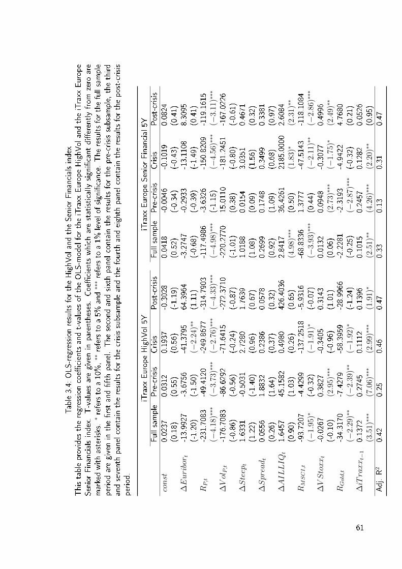
Table3.4:
OLS-regressionresultsfortheHighVol
andtheSeniorFinancialsindex
Thistableprovides
theregression
coe
cients
andt-values
oftheOLS-m
odelfortheiTraxx
EuropeHighVol
andtheiTraxx
Europe
SeniorFinancialsindex.T-values
aregivenin
parentheses.Coe
cients
whicharestatistically
signicantdierentlyfrom
zero
are
markedwithasterisks.∗refersto
a10%,∗∗refersto
a5%
and∗∗∗refersto
a1%
levelof
signicance.Theresultsforthefullsample
periodaregivenin
therstandfthpanel.Thesecondandsixthpanelcontain
theresultsforthepre-crisissubsample,thethird
andseventh
panelcontain
theresultsforthecrisissubsampleandthefourthandeighth
panelcontain
theresultsforthepost-crisis
period.
iTraxx
EuropeHighVol
5YiTraxx
EuropeSeniorFinancial5Y
Fullsample
Pre-crisis
Crisis
Post-crisis
Fullsample
Pre-crisis
Crisis
Post-crisis
const
0.0237
0.0312
0.1937
-0.3028
0.0418
-0.0046
-0.1019
0.0824
(0.18)
(0.55)
(0.56)
(-1.19)
(0.52)
(-0.34)
(-0.43)
(0.41)
∆Euribor t
-13.9927
-3.6756
-41.3795
64.3964
-3.2747
-0.2933
-13.1108
8.3095
(-1.20)
(-1.50)
(−2.
24)∗∗
(1.11)
(-0.68)
(-0.39)
(-1.49)
(0.41)
RP,t
-231.7083
-49.4120
-249.8677
-314.7903
-117.4986
-3.6326
-150.8209
-119.1615
(−4.
18)∗∗∗
(−3.
73)∗∗∗
(−2.
76)∗∗∗
(−4.
33)∗∗∗
(−4.
98)∗∗∗
(-1.15)
(−4.
56)∗∗∗
(−3.
11)∗∗∗
∆VolP,t
-176.7083
-86.6292
-71.6415
-272.3710
-220.2770
15.0110
-181.2451
-167.0226
(-0.86)
(-0.56)
(-0.24)
(-0.87)
(-1.01)
(0.38)
(-0.80)
(-0.61)
∆Steep
t1.6331
-0.5031
2.7280
1.7639
1.0188
0.0154
3.0351
0.4671
(1.22)
(-1.40)
(0.96)
(0.67)
(1.08)
(0.09)
(1.56)
(0.32)
∆Spreadt
0.0556
1.8832
0.2386
0.0578
0.2699
0.1748
0.3499
0.3381
(0.26)
(1.64)
(0.37)
(0.32)
(0.92)
(1.09)
(0.68)
(0.97)
∆AILLIQt
1.6457
45.1582
0.4980
426.4036
2.8417
36.4261
2185.0000
2.6084
(0.90)
(1.03)
(0.26)
(0.65)
(4.9
8)∗∗∗
(0.50)
(1.8
3)∗
(2.3
1)∗∗
RMSCI,t
-93.7207
-4.4299
-137.2518
-5.9316
-68.8336
1.3777
-47.5143
-118.1084
(−1.
95)∗
(-0.32)
(−1.
91)∗
(-0.07)
(−3.
93)∗∗∗
(0.44)
(−2.
11)∗∗
(−2.
86)∗∗∗
∆VStoxxt
-0.0267
0.3827
-0.3405
0.3143
0.0132
0.0948
-0.3077
0.4996
(-0.10)
(2.9
5)∗∗∗
(-0.96)
(1.01)
(0.06)
(2.7
3)∗∗∗
(−1.
75)∗
(2.4
9)∗∗
RGold,t
-34.3170
-7.4279
-58.3959
-28.9966
-2.2281
-2.3193
-4.9422
4.7680
(−2.
29)∗∗
(−2.
39)∗∗
(−1.
92)∗
(-1.24)
(-0.25)
(−2.
87)∗∗∗
(-0.32)
(0.21)
∆iTraxxt−
10.1372
0.2745
0.1112
0.1396
0.1015
0.2457
0.1282
0.0526
(3.5
1)∗∗∗
(7.0
6)∗∗∗
(2.9
9)∗∗∗
(1.9
1)∗
(2.5
1)∗∗
(4.2
6)∗∗∗
(2.2
0)∗∗
(0.95)
Adj.R2
0.42
0.25
0.46
0.47
0.33
0.13
0.31
0.47
61
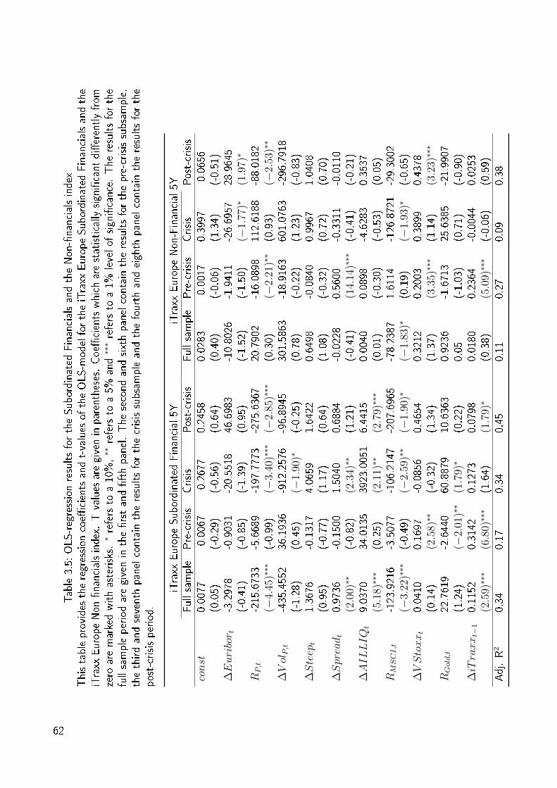
Table3.5:
OLS-regressionresultsfortheSubordinated
FinancialsandtheNon-nancialsindex
Thistableprovides
theregression
coe
cientsandt-values
oftheOLS-m
odelfortheiTraxx
EuropeSubordinated
Financialsandthe
iTraxx
EuropeNon-nancialsindex.T-values
aregiveninparentheses.Coe
cientswhicharestatistically
signicantdierentlyfrom
zero
aremarkedwithasterisks.∗refers
toa10%,∗∗
refers
toa5%
and∗∗∗refers
toa1%
levelof
signicance.Theresultsforthe
fullsampleperiodaregivenin
therstandfthpanel.Thesecondandsixthpanelcontain
theresultsforthepre-crisissubsample,
thethirdandseventh
panelcontaintheresultsforthecrisissubsampleandthefourthandeighth
panelcontain
theresultsforthe
post-crisisperiod.
iTraxx
EuropeSubordinated
Financial5Y
iTraxx
EuropeNon-Financial5Y
Fullsample
Pre-crisis
Crisis
Post-crisis
Fullsample
Pre-crisis
Crisis
Post-crisis
const
0.0077
-0.0067
-0.2677
0.2458
0.0283
-0.0017
0.3997
-0.0656
(0.05)
(-0.29)
(-0.56)
(0.64)
(0.40)
(-0.06)
(1.34)
(-0.51)
∆Euribor t
-3.2978
-0.9031
-20.5518
46.6983
-10.8026
-1.9411
-26.6957
28.9645
(-0.41)
(-0.85)
(-1.39)
(0.95)
(-1.52)
(-1.50)
(−1.
77)∗
(1.9
7)∗
RP,t
-215.6733
-5.6689
-197.7773
-275.6367
20.7902
-16.0898
112.6188
-88.0182
(−4.
45)∗∗∗
(-0.99)
(−3.
40)∗∗∗
(−2.
85)∗∗∗
(0.30)
(−2.
21)∗∗
(0.93)
(−2.
53)∗∗
∆VolP,t
-435.4552
36.1936
-912.2576
-96.8945
301.5863
-18.9163
601.0763
-296.7918
(-1.28)
(0.45)
(−1.
90)∗
(-0.25)
(0.78)
(-0.22)
(1.23)
(-0.83)
∆Steep
t1.3676
-0.1317
4.0659
1.6422
0.6498
-0.0840
0.9967
1.0408
(0.95)
(-0.77)
(1.17)
(0.64)
(1.08)
(-0.32)
(0.72)
(0.70)
∆Spreadt
0.9736
-0.1500
1.5040
0.6884
-0.0228
0.5600
-0.3311
-0.0110
(2.0
0)∗∗
(-0.82)
(2.3
4)∗∗
(1.21)
(-0.41)
(14.
14)∗∗∗
(-0.41)
(-0.21)
∆AILLIQt
9.0370
34.0135
3923.0051
6.4415
0.0040
0.0898
-4.6283
0.3537
(5.1
8)∗∗∗
(0.25)
(2.1
1)∗∗
(2.7
9)∗∗∗
(0.01)
(-0.30)
(-0.53)
(0.05)
RMSCI,t
-123.9216
-3.5077
-106.2147
-207.6965
-78.2387
1.6114
-126.8721
-29.3002
(−3.
22)∗∗∗
(-0.49)
(−2.
59)∗∗
(−1.
90)∗
(−1.
83)∗
(0.19)
(−1.
93)∗
(-0.65)
∆VStoxxt
0.0410
0.1697
-0.0856
0.4654
0.3212
0.2003
0.3899
0.4378
(0.14)
(2.5
8)∗∗
(-0.32)
(1.34)
(1.37)
(3.3
5)∗∗∗
(1.14)
(3.2
3)∗∗∗
RGold,t
22.7619
-2.6440
60.8879
10.6363
0.9236
-1.6713
25.6385
-21.9907
(1.24)
(−2.
01)∗∗
(1.7
9)∗
(0.22)
0.05
(-1.03)
(0.71)
(-0.90)
∆iTraxxt−
10.1152
0.3142
0.1273
0.0798
0.0180
0.2364
-0.0044
0.0253
(2.5
9)∗∗∗
(6.8
0)∗∗∗
(1.64)
(1.7
9)∗
(0.38)
(5.0
9)∗∗∗
(-0.06)
(0.59)
Adj.R2
0.34
0.17
0.34
0.45
0.11
0.27
0.09
0.38
62
The results obtained from the regression analysis for the dierent subindices of the iTraxx
Europe benchmark index are in many respects similar to the ones of the benchmark index.
There is empirical evidence that stock returns are the major determinant of iTraxx spread
changes. Stock market returns prove to be statistically signicant in twelve out of 16 regres-
sions for the dierent subindices. The other factors implied by structural models do not play
such an important role as the stock market factor. Changes in the Euribor rate are signicant
in only three out of 16 cases. The steepness of the risk-free curve has no statistically inu-
ence for all subsamples and subindices. Implied equity volatility has a statistically signicant
inuence in seven out of 16 cases. Again, previous ndings of related empirical studies that
credit spreads are especially sensitive towards volatility in times of crises are not conrmed.
Illiquidity eects are more pronounced for the subindices than for the benchmark index.
Equity market illiquidity is priced in the Senior Financials index, as well as in the Subordinated
Financials index. In contrast, equity market illiquidity has no statistically signicant inuence
on the HighVol and the Non-Financials index. This results suggest that hedging needs of
investors are especially pronounced when credit risk of nancial institutions is borne. In line
with the theoretical arguments provided by Das and Hanouna (2009), rising illiquidity in equity
markets causes credit spreads to rise, as it makes hedging more expensive. The inuence of
equity market illiquidity is stronger within the crisis and post-crisis sample than in the pre-
crisis sample, suggesting that illiquidity had a crucial role in the recent nancial crisis. The
fact that the sensitivity of iTraxx spread changes towards stock market liquidity is even more
pronounced after the crisis suggests that market participants have altered their perception of
the impact of stock liquidity on aggregate credit risk and have therefore altered their models
as a consequence of the crisis. Illiquidity in the market for credit risk, as measured by the
bid-ask spread of the respective index, does not have a signicant inuence except for the
iTraxx Non-Financials index. This conrms that the iTraxx Non-nancials index is generally
the most illiquid of the subindices.
The results for the other independent variables are in line with the results for the benchmark
index. Both the state of the global economy, as measured by the MSCI World index returns
and gold price changes, are signicantly related to credit spread changes. However, the eect
of gold price changes is most pronounced during the pre-crisis period. In general, the additional
explanatory power of the global nancial variables is small compared to the stock returns and
volatility and the gain from including them into a model of aggregate credit risk, which already
accounts for stock returns, is minor.
Similar to the benchmark index the degree of autocorrelation in spread changes declines
throughout the sample for all subindices. In the pre-crisis period, all subindices show statis-
63

tically signicant positive autocorrelation. This suggests that the subindices underreact to
new information, which can be interpreted as a lack of liquidity in the early years of the index
family, which steadily declines as the iTraxx matures. During the post-crisis period only the
iTraxx HighVol index shows signicant autocorrelation. This suggests that the eciency of
the iTraxx index universe has risen signicantly since the start of the index in 2004.
The results for the dierent subindices conrm the presence of variation in the determinants
of iTraxx spread changes. As observed for the benchmark index, the degree of determination
rises throughout the dierent subsamples, reaching the highest levels for the post-crisis period.
In contrast, the number of factors necessary to explain spread changes seems to decline through
time. In the post-crisis samples most of the variation in iTraxx spreads is explained by stock
returns and implied stock market volatility, while other factors have limited or no inuence.
3.6.2 Quantile Regression Results
In order to assess the robustness of the results obtained in the OLS-regression analysis in
the upper and lower quantiles of the empirical distribution of spread changes we perform
a quantile regression.7 This approach allows us to assess the performance of our set of
explanatory variables in predicting spread changes in upper and lower quantiles of the empirical
distribution. In other words, we analyze whether our set of explanatory variables is suited to
predict large spread changes, either positive or negative. For our purpose we estimate the
linear model described by equation (3.5) via quantile regression for the 0.25, the 0.50 and
the 0.75 quantile of the empirical distribution. The results for the dierent subindices and
subsamples are presented in Tables 3.6 to 3.10.
The results of the quantile regression are in many respects similar to the results of the
OLS-regression. The return on the stock portfolio of index constituents is the predominant
determinant of iTraxx spread changes. This result is robust for all quantiles and all subindices
and subsamples, and statistically highly signicant in almost every case. The regression coef-
cient generally is the highest for the upper 0.75 quantile, i.e. large spread widenings, except
for the post-crisis period. This nding suggests that the dependence between asset classes has
asymmetric features and is especially pronounced in downturns.
The results of the quantile regression conrm the results of the OLS-regression concerning
the presence of varying determinants within the complete sample. Comparing the post-crisis
sample results to the ones for pre-crisis sample, there is empirical evidence that dierent
7This approach was introduced by Koenker and Bassett (1978). According to Koenker and Hallock (2001)quantile regression models are models which express quantiles of the conditional distribution of the depen-dent variable as a function of observed covariates.
64
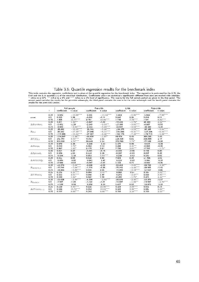
Table 3.6: Quantile regression results for the benchmark indexThis table contains the regression coecients and t-values of the quantile regression for the benchmark index. The regression is performed for the 0.25, the0.50 and the 0.75 quantile (τ) of the empirical distribution. Coecients which are statistically signicantly dierent from zero are marked with asterisks.∗ refers to a 10%, ∗∗ refers to a 5% and ∗∗∗ refers to a 1% level of signicance. The results for the full sample period are given in the rst panel. Thesecond panel contains the results for the pre-crisis subsample, the third panel contains the results for the crisis subsample and the fourth panel contains theresults for the post-crisis period.
Full sample Pre-crisis Crisis Post-crisisτ coecient t-value coecient t-value coecient t-value coecient t-value
0.25 -0.852 −13.69∗∗∗ -0.261 −11.54∗∗∗ -1.816 −5.90∗∗∗ -1.503 −7.88∗∗∗
const 0.5 0.053 1.39 -0.002 -0.11 0.042 0.26 0.016 0.110.75 1.005 15.77∗∗∗ 0.251 10.00∗∗∗ 1.739 7.78∗∗∗ 1.544 8.82∗∗∗
0.25 3.911 1.99∗∗ -0.947 -1.02 -18.443 −1.78∗ 46.490 2.92∗∗∗
∆Euribort 0.5 -2.051 -1.29 -2.240 −2.53∗∗ -17.300 −3.05∗∗∗ -8.007 -0.530.75 -8.868 −4.64∗∗∗ -2.413 −5.24∗∗∗ -23.697 −3.52∗∗∗ -26.360 -1.20
0.25 -85.882 −10.35∗∗∗ -28.341 −5.26∗∗∗ -136.375 −4.53∗∗∗ -95.395 −3.84∗∗∗
RP,t 0.5 -89.192 −17.49∗∗∗ -27.646 −6.11∗∗∗ -144.588 −8.31∗∗∗ -127.206 −6.34∗∗∗
0.75 -113.896 −13.34∗∗∗ -32.302 −6.36∗∗∗ -163.178 −7.49∗∗∗ -128.713 −5.08∗∗∗
0.25 -114.847 −1.98∗∗ -60.438 −1.87∗ 69.974 0.43 369.280 1.40∆V olP,t 0.5 131.754 3.53∗∗∗ 43.914 1.21 116.326 0.81 226.696 1.47
0.75 313.335 4.70∗∗∗ 58.645 1.14 272.783 1.73∗ -77.183 -0.39
0.25 0.578 1.16 -0.338 -1.32 1.179 0.48 -0.625 -0.38∆Steept 0.5 0.610 1.73∗ 0.024 0.12 2.496 2.21∗∗ -0.388 -0.30
0.75 0.862 1.65∗ 0.125 0.64 2.700 2.61∗∗ -2.785 −1.71∗
0.25 0.021 0.37 -0.041 -0.15 -0.330 -0.86 0.135 0.50∆Spreadt 0.5 0.059 1.04 0.114 0.39 -0.207 -0.93 0.037 0.15
0.75 -0.104 -1.19 0.853 5.84∗∗∗ -0.226 -0.93 0.143 0.61
0.25 0.011 0.04 0.018 0.92 7.929 0.35 14.796 1.61∆AILLIQt 0.5 -0.056 -0.55 -0.042 -1.47 -0.123 -0.02 -2.384 -0.35
0.75 -0.088 -0.53 -0.047 -1.07 1.125 0.71 -4.442 -0.36
0.25 -46.574 −5.08∗∗∗ -3.038 -0.55 -59.413 −3.05∗∗∗ -58.733 −2.29∗∗
RMSCI,t 0.5 -37.745 −7.08∗∗∗ -1.318 -0.28 -70.342 −4.49∗∗∗ -29.865 -1.420.75 -49.893 −5.89∗∗∗ 0.039 0.01 -72.059 −3.18∗∗∗ -17.517 -0.66
0.25 0.235 6.21∗∗∗ 0.084 2.31∗∗ -0.090 -0.54 0.397 3.02∗∗∗
∆V Stoxxt 0.5 0.163 4.61∗∗∗ 0.048 1.47 -0.273 −2.47∗∗ 0.430 3.95∗∗∗
0.75 0.100 1.84∗ 0.060 1.56 -0.285 −1.75∗ 0.471 4.44∗∗∗
0.25 -11.018 −2.90∗∗∗ -4.204 −2.84∗∗∗ -35.570 −2.40∗∗ -15.376 -1.17RGold,t 0.5 -3.887 -1.48 -1.422 -1.01 -16.887 −1.98∗∗ -19.957 −2.70∗∗∗
0.75 -4.198 -0.99 -0.390 -0.23 1.427 0.12 -18.871 -1.39
0.25 0.119 9.85∗∗∗ 0.210 22.86∗∗∗ 0.129 3.08∗∗∗ 0.031 0.73∆iTraxxt−1 0.5 0.134 15.72∗∗∗ 0.214 10.04∗∗∗ 0.105 3.96∗∗∗ 0.064 2.00∗∗
0.75 0.107 9.69∗∗∗ 0.242 9.86∗∗∗ 0.100 3.10∗∗∗ 0.100 2.55∗∗
65
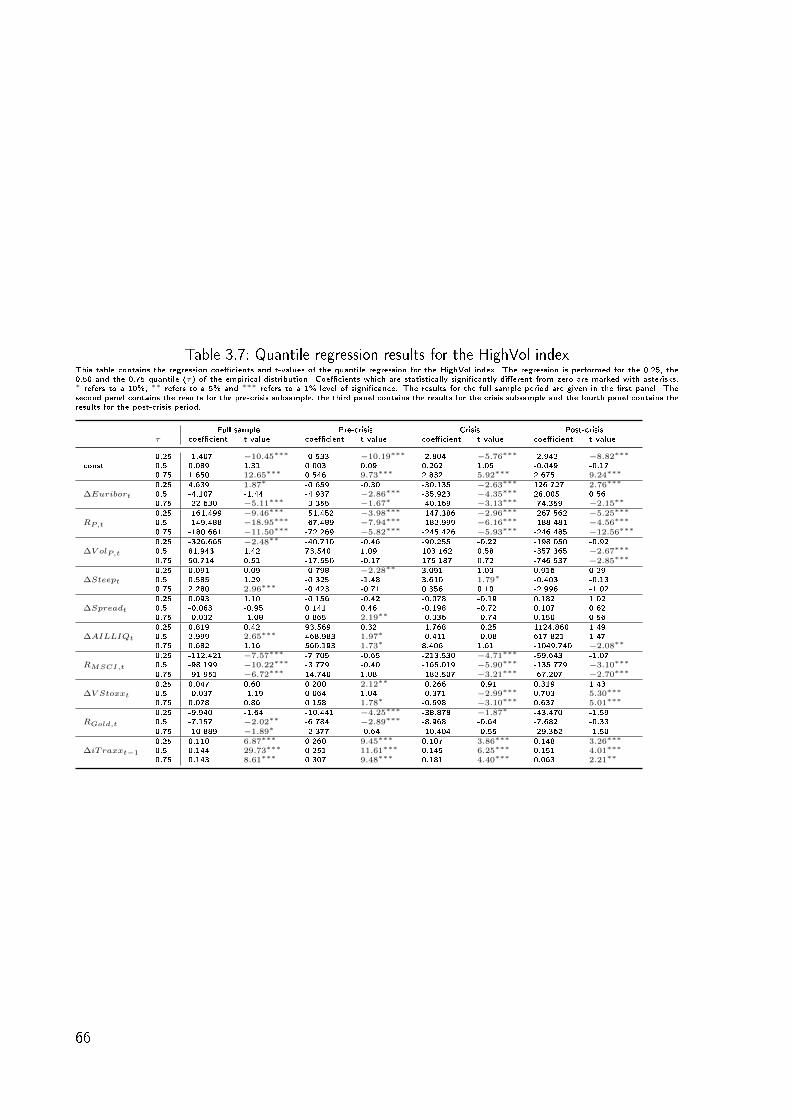
Table 3.7: Quantile regression results for the HighVol indexThis table contains the regression coecients and t-values of the quantile regression for the HighVol index. The regression is performed for the 0.25, the0.50 and the 0.75 quantile (τ) of the empirical distribution. Coecients which are statistically signicantly dierent from zero are marked with asterisks.∗ refers to a 10%, ∗∗ refers to a 5% and ∗∗∗ refers to a 1% level of signicance. The results for the full sample period are given in the rst panel. Thesecond panel contains the results for the pre-crisis subsample, the third panel contains the results for the crisis subsample and the fourth panel contains theresults for the post-crisis period.
Full sample Pre-crisis Crisis Post-crisisτ coecient t-value coecient t-value coecient t-value coecient t-value
0.25 -1.407 −10.45∗∗∗ -0.533 −10.19∗∗∗ -2.804 −5.76∗∗∗ -2.942 −8.82∗∗∗
const 0.5 0.089 1.31 0.003 0.09 0.262 1.05 -0.049 -0.170.75 1.650 12.65∗∗∗ 0.546 9.73∗∗∗ 2.832 5.92∗∗∗ 2.675 9.24∗∗∗
0.25 4.639 1.87∗ -0.659 -0.30 -30.135 −2.63∗∗∗ 126.727 2.76∗∗∗
∆Euribort 0.5 -4.107 -1.44 -4.937 −2.86∗∗∗ -35.923 −4.35∗∗∗ 28.005 0.560.75 -22.630 −5.11∗∗∗ -3.355 −1.67∗ -40.169 −3.13∗∗∗ -74.359 −2.15∗∗
0.25 -161.499 −9.46∗∗∗ -51.452 −3.98∗∗∗ -147.386 −2.96∗∗∗ -267.562 −5.25∗∗∗
RP,t 0.5 -149.488 −18.95∗∗∗ -67.489 −7.94∗∗∗ -182.999 −6.16∗∗∗ -188.481 −4.56∗∗∗
0.75 -180.661 −11.50∗∗∗ -72.269 −5.82∗∗∗ -245.426 −5.93∗∗∗ -246.485 −12.56∗∗∗
0.25 -326.665 −2.48∗∗ -40.710 -0.46 -90.255 -0.22 -198.050 -0.92∆V olP,t 0.5 81.943 1.42 73.540 1.09 103.162 0.58 -357.365 −2.67∗∗∗
0.75 50.714 0.51 -17.550 -0.17 175.187 0.72 -746.537 −2.85∗∗∗
0.25 0.091 0.09 -0.798 −2.28∗∗ 3.091 1.03 0.916 0.29∆Steept 0.5 0.585 1.29 -0.325 -1.48 3.610 1.79∗ -0.403 -0.13
0.75 2.280 2.96∗∗∗ -0.423 -0.71 0.356 0.10 -2.996 -1.02
0.25 0.093 1.10 -0.156 -0.42 -0.078 -0.19 0.182 1.02∆Spreadt 0.5 -0.063 -0.95 0.141 0.46 -0.198 -0.72 0.107 0.62
0.75 -0.032 -1.08 0.865 2.19∗∗ -0.336 -0.74 0.150 0.56
0.25 0.819 0.42 93.569 0.32 -1.768 -0.25 1124.860 1.49∆AILLIQt 0.5 2.999 2.65∗∗∗ 468.983 1.97∗ -0.411 -0.08 617.821 1.47
0.75 0.682 1.16 560.193 1.73∗ 8.406 1.61 -1049.740 −2.08∗∗
0.25 -112.421 −7.57∗∗∗ -7.705 -0.65 -213.530 −4.71∗∗∗ -59.643 -1.07RMSCI,t 0.5 -98.199 −10.22∗∗∗ -3.779 -0.40 -165.019 −5.90∗∗∗ -135.779 −3.10∗∗∗
0.75 -91.951 −6.72∗∗∗ 14.740 1.08 -182.507 −3.21∗∗∗ -67.207 −2.70∗∗∗
0.25 0.047 0.60 0.200 2.12∗∗ -0.266 -0.91 0.319 1.43∆V Stoxxt 0.5 -0.037 -1.19 0.064 1.04 -0.371 −2.99∗∗∗ 0.703 5.30∗∗∗
0.75 0.078 0.86 0.158 1.78∗ -0.698 −3.10∗∗∗ 0.637 5.01∗∗∗
0.25 -9.940 -1.64 -10.441 −4.25∗∗∗ -38.878 −1.87∗ -43.470 -1.59RGold,t 0.5 -7.157 −2.02∗∗ -6.784 −2.89∗∗∗ -8.968 -0.64 -7.682 -0.33
0.75 -10.889 −1.89∗ -2.377 -0.64 -10.404 -0.55 -29.362 -1.50
0.25 0.110 6.87∗∗∗ 0.260 9.45∗∗∗ 0.107 3.86∗∗∗ 0.148 3.26∗∗∗
∆iTraxxt−1 0.5 0.144 29.73∗∗∗ 0.251 11.61∗∗∗ 0.145 6.25∗∗∗ 0.151 4.01∗∗∗
0.75 0.143 8.61∗∗∗ 0.307 9.48∗∗∗ 0.181 4.40∗∗∗ 0.063 2.21∗∗
66
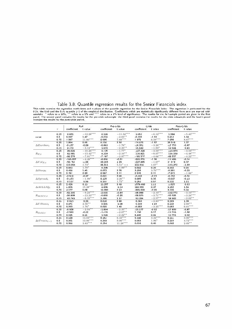
Table 3.8: Quantile regression results for the Senior Financials indexThis table contains the regression coecients and t-values of the quantile regression for the Senior Financials index. The regression is performed for the0.25, the 0.50 and the 0.75 quantile (τ) of the empirical distribution. Coecients which are statistically signicantly dierent from zero are marked withasterisks. ∗ refers to a 10%, ∗∗ refers to a 5% and ∗∗∗ refers to a 1% level of signicance. The results for the full sample period are given in the rstpanel. The second panel contains the results for the pre-crisis subsample, the third panel contains the results for the crisis subsample and the fourth panelcontains the results for the post-crisis period.
Full Pre-crisis Crisis Post-Crisisτ coecient t-value coecient t-value coecient t-value coecient t-value
0.25 -0.851 −12.28∗∗∗ -0.128 −11.34∗∗∗ -2.052 −6.12∗∗∗ -1.566 −5.43∗∗∗
const 0.5 0.057 1.47 -0.016 −2.05∗∗ -0.190 -1.00 0.212 1.180.75 1.067 11.80∗∗∗ 0.099 7.88∗∗∗ 1.970 6.59∗∗∗ 2.056 8.67∗∗∗
0.25 1.994 0.95 0.136 0.30 -14.675 -1.57 26.048 1.37∆Euribort 0.5 -0.157 -0.09 -0.663 −1.76∗ -18.351 −3.28∗∗∗ -17.753 -0.87
0.75 -8.770 −3.12∗∗∗ -1.070 −2.35∗∗ -15.588 −1.93∗ -10.584 -0.65
0.25 -86.028 −10.26∗∗∗ -4.435 −1.77∗ -127.329 −3.59∗∗∗ -114.974 −3.59∗∗∗
RP,t 0.5 -62.981 −13.42∗∗∗ -4.314 −2.10∗∗ -120.621 −8.07∗∗∗ -116.150 −4.48∗∗∗
0.75 -88.579 −7.91∗∗∗ -7.467 −2.97∗∗∗ -160.522 −4.66∗∗∗ -99.557 −4.22∗∗∗
0.25 -160.057 −4.49∗∗∗ -8.806 -0.51 -260.076 -1.36 -14.456 -0.14∆V olP,t 0.5 -50.452 -1.08 20.205 1.29 -227.885 −1.67∗ 34.049 0.37
0.75 113.954 1.73∗ 48.311 5.51∗ ∗ ∗ 222.916 1.67∗ -141.372 -1.59
0.25 0.843 1.70∗ -0.206 −1.99∗∗ 0.503 0.20 0.392 0.16∆Steept 0.5 0.436 1.45 0.072 0.76 3.288 3.70∗∗∗ -0.381 -0.23
0.75 0.491 0.89 0.062 0.41 0.940 0.41 -2.843 −1.86∗
0.25 -0.042 -0.37 0.041 0.66 -0.242 -0.73 -0.132 -0.34∆Spreadt 0.5 -0.153 −1.99∗ 0.125 2.26∗∗ 0.095 0.35 -0.037 -0.13
0.75 -0.117 -0.98 0.107 1.72∗ 0.263 0.57 0.332 1.11
0.25 2.426 0.13 13.257 0.48 1579.460 1.11 -1.025 -0.03∆AILLIQt 0.5 4.896 15.28∗∗∗ -4.096 -0.14 362.955 0.37 3.252 1.54
0.75 2.177 0.09 12.090 0.22 -866.668 -0.66 3.135 0.22
0.25 -62.165 −9.24∗∗∗ -2.015 -0.84 -66.968 −2.10∗∗ -102.772 −3.10∗∗∗
RMSCI,t 0.5 -50.909 −13.33∗∗∗ -0.600 -0.28 -59.870 −3.71∗∗∗ -90.555 −3.24∗∗∗
0.75 -63.743 −6.33∗∗∗ 3.380 1.17 -63.284 −2.57∗∗ -56.883 −2.02∗∗
0.25 -0.013 -0.28 0.016 0.90 -0.393 −2.83∗∗∗ 0.209 1.39∆V Stoxxt 0.5 0.071 2.56∗∗ -0.001 -0.06 -0.104 -1.05 0.232 2.60∗∗
0.75 0.093 1.76∗ 0.025 1.45 -0.383 −3.25∗∗∗ 0.683 6.01∗∗∗
0.25 -6.928 −2.04∗∗ -1.664 −2.35∗∗ -15.177 -0.92 -17.850 -0.87RGold,t 0.5 -0.560 -0.22 -1.418 −2.07∗∗ 1.130 0.17 -14.746 -1.08
0.75 0.935 0.21 -1.928 −2.22∗∗ 6.449 0.44 -13.791 -0.92
0.25 0.129 14.03∗∗∗ 0.167 6.43∗∗∗ 0.146 3.22∗∗∗ 0.114 3.00∗∗∗
∆iTraxxt−1 0.5 0.091 13.06∗∗∗ 0.203 9.06∗∗∗ 0.055 1.96∗ 0.109 4.72∗∗∗
0.75 0.066 3.83∗∗∗ 0.254 11.28∗∗∗ 0.016 0.40 0.068 2.09∗∗
67
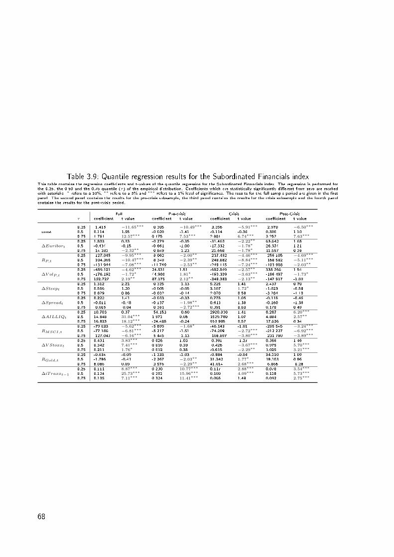
Table 3.9: Quantile regression results for the Subordinated Financials indexThis table contains the regression coecients and t-values of the quantile regression for the Subordinated Financials index. The regression is performed forthe 0.25, the 0.50 and the 0.75 quantile (τ) of the empirical distribution. Coecients which are statistically signicantly dierent from zero are markedwith asterisks. ∗ refers to a 10%, ∗∗ refers to a 5% and ∗∗∗ refers to a 1% level of signicance. The results for the full sample period are given in the rstpanel. The second panel contains the results for the pre-crisis subsample, the third panel contains the results for the crisis subsample and the fourth panelcontains the results for the post-crisis period.
Full Pre-crisis Crisis Post-Crisisτ coecient t-value coecient t-value coecient t-value coecient t-value
0.25 -1.415 −11.65∗∗∗ -0.205 −10.49∗∗∗ -3.256 −5.91∗∗∗ -2.970 −6.50∗∗∗
const 0.5 0.114 1.55 -0.020 -1.41 -0.114 -0.36 0.300 1.100.75 1.761 12.57∗∗∗ 0.175 7.53∗∗∗ 2.881 6.74∗∗∗ 3.252 7.63∗∗∗
0.25 1.803 0.33 -0.279 -0.35 -31.460 −2.22∗∗ 63.642 1.65∆Euribort 0.5 -0.434 -0.15 -0.661 -1.00 -17.332 −1.78∗ 26.374 1.21
0.75 -14.381 −2.32∗∗ -0.849 -1.23 -21.668 −1.78∗ 11.557 0.26
0.25 -127.845 −9.95∗∗∗ -8.062 −2.00∗∗ -237.462 −4.46∗∗∗ -256.105 −4.69∗∗∗
RP,t 0.5 -104.365 −10.47∗∗∗ -8.240 −2.39∗∗ -248.862 −8.84∗∗∗ -168.582 −5.11∗∗∗
0.75 -131.944 −7.08∗∗∗ -11.749 −2.53∗∗ -249.115 −7.24∗∗∗ -103.908 −2.03∗∗
0.25 -459.121 −4.62∗∗∗ 24.531 1.51 -682.849 −2.57∗∗ 335.766 1.54∆V olP,t 0.5 -176.192 −1.72∗ 44.980 1.81∗ -493.309 −3.63∗∗∗ -186.497 −1.73∗
0.75 152.727 2.19∗∗ 87.175 2.12∗∗ -349.383 −2.13∗∗ -147.917 -1.00
0.25 1.312 2.21 -0.225 -1.13 5.225 1.41 2.437 0.70∆Steept 0.5 0.566 1.20 -0.005 -0.05 3.107 1.72∗ -1.023 -0.59
0.75 0.829 0.86 -0.032 -0.14 2.070 0.58 -3.284 -1.10
0.25 0.222 1.41 -0.033 -0.33 0.778 1.05 -0.118 -0.46∆Spreadt 0.5 -0.011 -0.48 -0.137 −1.98∗∗ 0.613 1.38 -0.160 -1.36
0.75 -0.005 -0.04 -0.261 −2.72∗∗∗ 0.391 0.80 0.178 0.49
0.25 10.703 0.37 -54.153 -0.60 2920.830 1.41 8.287 6.20∗∗∗
∆AILLIQt 0.5 14.848 31.04∗∗∗ 1.971 0.06 1529.780 1.07 4.884 2.57∗∗
0.75 16.833 18.12∗∗∗ -24.488 -0.24 910.995 0.57 17.626 0.34
0.25 -79.033 −5.62∗∗∗ -5.699 −1.68∗ -46.143 -1.01 -205.545 −3.24∗∗∗
RMSCI,t 0.5 -77.186 −6.81∗∗∗ -5.217 -1.51 -74.209 −2.72∗∗∗ -212.227 −6.92∗∗∗
0.75 -127.047 −6.16∗∗∗ -5.445 -1.13 -106.897 −3.80∗∗∗ -231.760 −3.89∗∗∗
0.25 0.431 3.83∗∗∗ 0.026 1.03 -0.391 -1.27 0.366 1.46∆V Stoxxt 0.5 0.342 7.41∗∗∗ 0.010 0.39 -0.426 −3.67∗∗∗ 0.975 5.70∗∗∗
0.75 0.211 1.76∗ 0.012 0.38 -0.615 −2.29∗∗ 1.025 3.21∗∗∗
0.25 -0.634 -0.09 -1.233 -1.03 -0.684 -0.04 34.110 1.09RGold,t 0.5 -1.796 -0.41 -2.267 −2.03∗∗ 31.342 1.77∗ 19.103 0.96
0.75 6.066 0.69 -3.576 −2.29∗∗ 41.014 2.68∗∗∗ -6.666 -0.26
0.25 0.111 8.87∗∗∗ 0.230 10.77∗∗∗ 0.117 2.88∗∗∗ 0.078 3.54∗∗∗
∆iTraxxt−1 0.5 0.124 25.73∗∗∗ 0.251 15.96∗∗∗ 0.100 4.09∗∗∗ 0.116 5.73∗∗∗
0.75 0.105 7.11∗∗∗ 0.324 11.41∗∗∗ 0.068 1.49 0.092 2.75∗∗∗
68
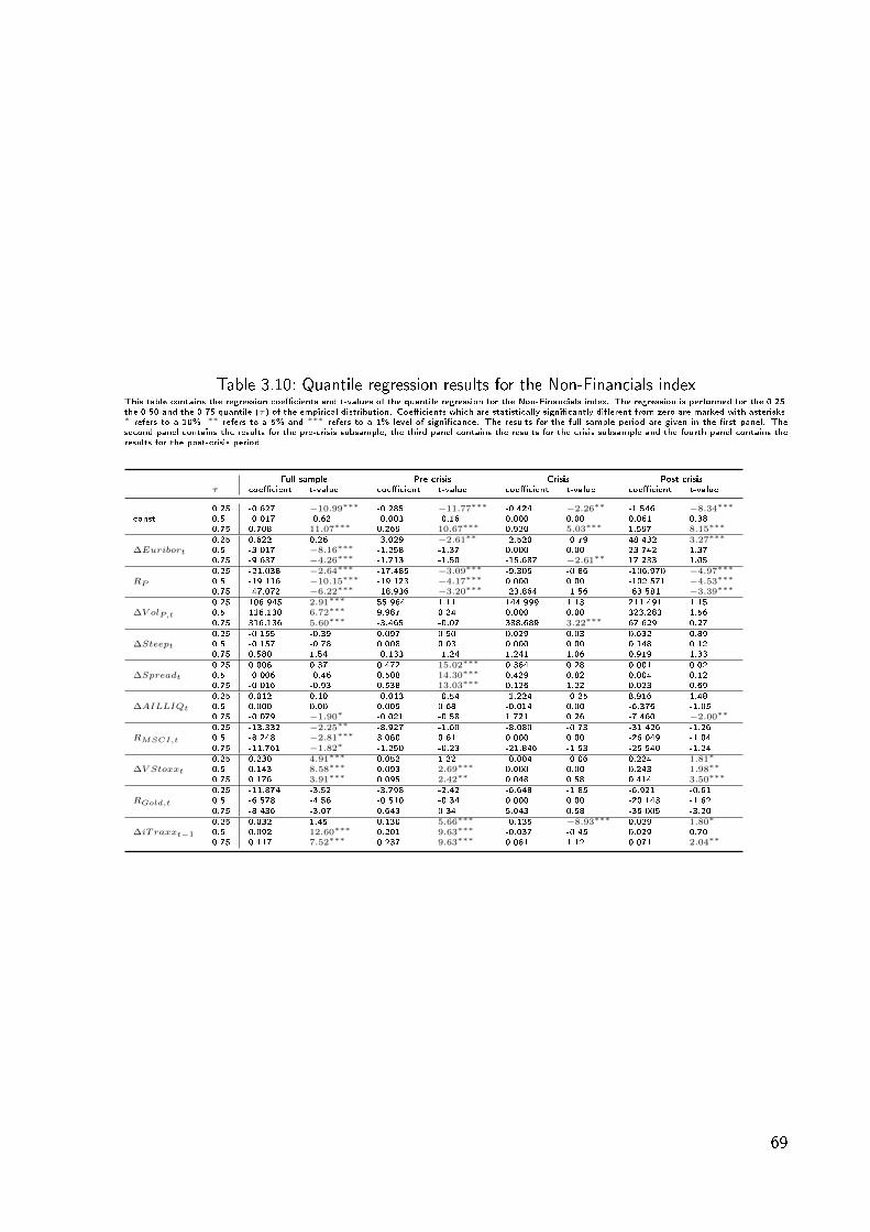
Table 3.10: Quantile regression results for the Non-Financials indexThis table contains the regression coecients and t-values of the quantile regression for the Non-Financials index. The regression is performed for the 0.25,the 0.50 and the 0.75 quantile (τ) of the empirical distribution. Coecients which are statistically signicantly dierent from zero are marked with asterisks.∗ refers to a 10%, ∗∗ refers to a 5% and ∗∗∗ refers to a 1% level of signicance. The results for the full sample period are given in the rst panel. Thesecond panel contains the results for the pre-crisis subsample, the third panel contains the results for the crisis subsample and the fourth panel contains theresults for the post-crisis period.
Full sample Pre-crisis Crisis Post-crisisτ coecient t-value coecient t-value coecient t-value coecient t-value
0.25 -0.627 −10.99∗∗∗ -0.285 −11.77∗∗∗ -0.424 −2.26∗∗ -1.546 −8.34∗∗∗
const 0.5 -0.017 -0.62 -0.003 -0.16 0.000 0.00 0.061 0.380.75 0.708 11.07∗∗∗ 0.269 10.67∗∗∗ 0.920 5.03∗∗∗ 1.597 8.15∗∗∗
0.25 0.622 0.26 -3.029 −2.61∗∗ -2.520 -0.79 48.432 3.27∗∗∗
∆Euribort 0.5 -3.017 −8.16∗∗∗ -1.258 -1.37 0.000 0.00 23.742 1.370.75 -9.637 −4.26∗∗∗ -1.713 -1.50 -15.687 −2.61∗∗ 17.233 1.05
0.25 -21.038 −2.64∗∗∗ -17.485 −3.09∗∗∗ -9.305 -0.86 -106.970 −4.97∗∗∗
RP 0.5 -19.116 −10.15∗∗∗ -19.123 −4.17∗∗∗ 0.000 0.00 -102.571 −4.53∗∗∗
0.75 -47.072 −6.22∗∗∗ -18.936 −3.20∗∗∗ -23.864 -1.56 -63.581 −3.39∗∗∗
0.25 106.945 2.91∗∗∗ 55.964 1.11 144.999 1.13 211.491 1.15∆V olP,t 0.5 116.130 6.72∗∗∗ 9.987 0.24 0.000 0.00 323.283 1.56
0.75 316.136 5.60∗∗∗ -3.465 -0.07 388.689 3.22∗∗∗ 67.629 0.27
0.25 -0.155 -0.39 0.097 0.50 0.029 0.03 0.632 0.89∆Steept 0.5 -0.157 -0.78 0.008 0.03 0.000 0.00 0.148 0.12
0.75 0.580 1.54 -0.133 -1.24 1.241 1.06 0.919 1.33
0.25 0.006 0.37 0.472 15.02∗∗∗ 0.384 0.28 0.001 0.02∆Spreadt 0.5 -0.006 -0.46 0.508 14.30∗∗∗ 0.429 0.82 0.004 0.12
0.75 -0.016 -0.93 0.538 13.03∗∗∗ 0.126 1.22 0.023 0.69
0.25 0.012 0.10 -0.013 -0.54 -1.224 -0.25 8.916 1.48∆AILLIQt 0.5 0.000 0.00 0.009 0.68 -0.014 0.00 -6.376 -1.05
0.75 -0.079 −1.90∗ -0.021 -0.58 1.721 0.26 -7.460 −2.00∗∗
0.25 -13.332 −2.25∗∗ -8.927 -1.60 -8.080 -0.73 -31.426 -1.26RMSCI,t 0.5 -8.248 −2.81∗∗∗ 3.060 0.61 0.000 0.00 -26.049 -1.04
0.75 -11.761 −1.82∗ -1.250 -0.23 -21.846 -1.53 -25.540 -1.24
0.25 0.230 4.91∗∗∗ 0.052 1.22 -0.004 -0.06 0.224 1.81∗
∆V Stoxxt 0.5 0.143 8.58∗∗∗ 0.093 2.69∗∗∗ 0.000 0.00 0.243 1.98∗∗
0.75 0.176 3.91∗∗∗ 0.095 2.42∗∗ 0.048 0.58 0.414 3.50∗∗∗
0.25 -11.874 -3.52 -3.798 -2.42 -6.648 -1.85 -6.921 -0.61RGold,t 0.5 -6.578 -4.56 -0.510 -0.34 0.000 0.00 -20.143 -1.62
0.75 -8.436 -3.07 0.643 0.34 5.043 0.58 -36.005 -3.20
0.25 0.032 1.45 0.130 5.66∗∗∗ -0.135 −8.93∗∗∗ 0.029 1.80∗
∆iTraxxt−1 0.5 0.092 12.60∗∗∗ 0.201 9.63∗∗∗ -0.037 -0.45 0.029 0.700.75 0.117 7.52∗∗∗ 0.237 9.63∗∗∗ 0.081 1.12 0.071 2.04∗∗
69

explanatory variables are signicant in the single subsamples. This points to the fact that
the pricing of the iTraxx by market participants has been reassessed in the light of the recent
credit crisis.
In addition to conrming the major results of the OLS-regression, the quantile regression
reveals some additional insights regarding the mechanics governing iTraxx spread changes. For
example, the volatility of the stock portfolio shows some remarkable results for the quantile
regression. When we look at the results for the full sample period (the rst panel of Tables 3.6-
3.10), there is a switch in the regression coecient between the upper and the lower quantile.
For the lower quantile the regression coecient carries the wrong sign from a theoretical
perspective. In general, the volatility is statistically signicant for several quantiles and seems
to be better suited in explaining large spread widenings than large spread tightenings. Hence,
it provides valuable information for upper and lower quantiles of spread changes, although it
is not signicant in the OLS-regression.
The interest rate factor, proxied by the Euribor rate, shows some nonlinearities as well. The
factor is statistically signicant in the upper quantile in almost all cases, except for the post-
crisis samples. In contrast, its predictive power is worse for the lower quantile, with the wrong
sign of the regression coecient in most cases. Just like the volatility of the equity portfolio,
the Euribor rate has predictive power for large spread widenings, while showing inconsistent
results for large spread tightenings.
The opposite is true for the gold price changes. Their statistical signicance is generally
higher in the lower quantile than in the upper quantile, i.e. gold price changes have higher
explanatory power for large spread tightenings than large spread widenings. However, the sign
of the regression coecient is negative and not in line with theory.
The liquidity variables, especially the proxy for equity market illiquidity, perform best around
the median of spread changes. Surprisingly, their predictive power in the upper and lower
quantiles is statistically not signicant, even for the subsamples and subindices where they
have a statistical signicant inuence in the OLS-regression.
A look at the regression results for the constant reveals another interesting feature of iTraxx
spread changes. In the preceding OLS-regression, the constant is not statistically dierent from
zero for all subsamples and all subindices. In the quantile regression, the picture is dierent.
The constant is statistically signicantly dierent from zero at the 1%-level for all upper and
all lower quantiles. This result is robust for all subsamples and all subindices. In contrast, the
constant is not statistically signicant dierent from zero for all median quantiles. It carries a
negative sign for all lower quantiles and a positive sign for all upper quantiles. This suggests
that our set of explanatory variables systematically underestimates large spread tightenings,
70
as well as large spread widenings.
This empirical nding leads to the conclusion that our set of explanatory variables is not able
to explain a signicant systematic fraction of spread changes in the upper and lower tail of the
empirical distribution. Additional factors seem to be necessary to explain spread changes at
the tails of the empirical distribution that are not implied by structural models. The liquidity
variables, which seem to be natural candidates for predicting extreme spread movements fail
to fulll this task, having no statistically signicant inuence in the upper and lower quantiles.
3.6.3 The Lead-Lag Relationship Between the Market for Credit
Risk and the Stock Market
In order to assess whether market participants use iTraxx Europe spreads as an additional
source of information regarding systemic risk, we examine the lead-lag relationship between
iTraxx spread changes and stock returns on the portfolio consisting of iTraxx constituents.
For this purpose we estimate a VARX-model. The exogenous variables used in the model are
supposed to jointly determine iTraxx spread changes, as well as stock returns. The set of
exogenous variables used in the preceding OLS-regression are natural candidates. As these
variables should in theory determine the creditworthiness of the index constituents, they in
turn should drive stock returns as well. The same is true for the hedging arguments related to
the liquidity variables. Using a VARX- instead of a simple VAR-model has the advantage that
no biases due to omitted variables arise. The econometric representation of the VARX-model
is of the form
∆iT raxxt = c1 +4∑i=1
β1,i∆iT raxxt−i +4∑i=1
γ1,iRP,t−i + λ1,1∆Euribort
+ λ1,2∆V olP,t + λ1,3∆Steept + λ1,4∆Spreadt + λ1,5∆AILLIQt
+ λ1,6RMSCI,t + λ1,7∆V Stoxx+ λ1,8RGold,t + ε1,t
RP,t = c2 +4∑i=1
β2,i∆iT raxxt−i +4∑i=1
γ2,iRP,t−i + λ2,1∆Euribort
+ λ2,2∆V olP,t + λ2,3∆Steept + λ2,4∆Spreadt + λ2,5∆AILLIQt
+ λ2,6RMSCI,t + λ2,7∆V Stoxx+ λ2,8RGold,t + ε2,t.
(3.6)
We choose a lag order of 4 lags, which is the model with the lowest value for the Hannan-
71
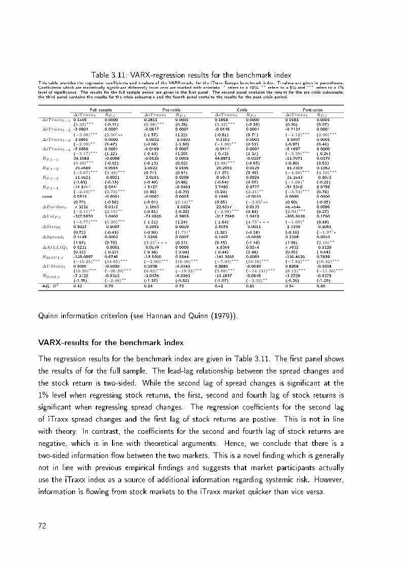
Table 3.11: VARX-regression results for the benchmark indexThis table provides the regression coecients and t-values of the VARX-model for the iTraxx Europe benchmark index. T-values are given in parentheses.Coecients which are statistically signicant dierently from zero are marked with asterisks. ∗ refers to a 10%, ∗∗ refers to a 5% and ∗∗∗ refers to a 1%level of signicance. The results for the full sample period are given in the rst panel. The second panel contains the results for the pre-crisis subsample,the third panel contains the results for the crisis subsample and the fourth panel contains the results for the post-crisis period.
Full sample Pre-crisis Crisis Post-crisis∆iTraxxt RP,t ∆iTraxxt RP,t ∆iTraxxt RP,t ∆iTraxxt RP,t
∆iTraxxt−1 0.1405 0.0000 0.2611 0.0001 0.1858 0.0000 0.0183 0.0001(5.33)∗∗∗ (-0.11) (6.98)∗∗∗ (0.28) (3.42)∗∗∗ (-0.28) (0.36) (0.97)
∆iTraxxt−2 -0.0904 0.0002 -0.0617 0.0002 -0.0449 0.0001 -0.2134 0.0004
(−3.38)∗∗∗ (2.50)∗∗ (-1.57) (1.22) (-0.81) (0.74) (−4.12)∗∗∗ (2.96)∗∗∗
∆iTraxxt−3 -0.0651 0.0000 -0.0022 -0.0003 -0.1153 0.0001 -0.0497 0.0001(−2.39)∗∗ (0.47) (-0.06) (-1.50) (−1.99)∗∗ (0.51) (-0.97) (0.46)
∆iTraxxt−4 -0.0858 0.0001 -0.0169 0.0002 -0.0414 0.0002 -0.1697 0.0000(−3.17)∗∗∗ (1.12) (-0.43) (1.20) (-0.73) (1.37) (−3.29)∗∗∗ (-0.25)
RP,t−1 24.1083 -0.0066 -0.5533 0.0003 44.8871 -0.0207 -11.7071 0.0179(3.49)∗∗∗ (-0.42) (-0.13) (0.02) (2.98)∗∗∗ (-0.65) (-0.80) (0.53)
RP,t−2 -25.4689 0.0555 3.0922 0.0195 -20.2091 0.0129 -61.7319 0.1363(−3.67)∗∗∗ (3.48)∗∗∗ (0.74) (0.91) (-1.32) (0.40) (−4.29)∗∗∗ (4.10)∗∗∗
RP,t−3 -11.5521 -0.0021 -2.0161 0.0209 -8.5873 0.0024 -24.1543 -0.0072(-1.63) (-0.13) (-0.48) (0.98) (-0.54) (0.07) (−1.68)∗ (-0.22)
RP,t−4 -14.8114 0.0444 1.5152 -0.0063 3.7480 0.0727 -54.5310 0.0256(−2.10)∗∗ (2.73)∗∗∗ (0.36) (-0.29) (0.24) (2.21)∗∗ (−3.74)∗∗∗ (0.76)
const 0.0514 -0.0001 -0.0002 0.0003 0.1946 -0.0010 0.0990 0.0000
(0.72) (-0.56) (-0.01) (2.14)∗∗ (0.85) (−2.05)∗∗ (0.60) (-0.05)∆Euribort -7.3211 0.0172 -1.1653 -0.0024 -22.6257 0.0133 45.4544 0.0096
(−2.11)∗∗ (2.15)∗∗ (-0.81) (-0.33) (−2.98)∗∗∗ (0.83) (2.94)∗∗∗ (0.27)∆V olP,t -327.5970 1.0400 -74.6520 0.3903 -317.7549 1.9413 -265.3628 0.1780
(−3.77)∗∗∗ (5.20)∗∗∗ (-1.21) (1.24) (-1.64) (4.75)∗ ∗ ∗ (−1.69)∗ (0.49)∆Steept 0.5027 -0.0007 -0.2953 0.0029 2.5078 -0.0011 -0.2199 -0.0061
(0.71) (-0.43) (-0.90) (1.71)∗ (1.30) (-0.28) (-0.16) (−1.97)∗∆Spreadt 0.1449 0.0002 1.3288 0.0007 0.1467 -0.0008 0.2229 0.0010
(1.04) (0.76) (3.21)∗ ∗ ∗ (0.31) (0.45) (-1.16) (1.05) (2.10)∗∗
∆AILLIQt 0.0211 -0.0001 -0.0179 0.0000 -4.8356 0.0244 4.7632 -0.0128(0.11) (-0.22) (-0.36) (-0.04) (-0.44) (1.06) (0.55) (-0.64)
RMSCI,t -128.0997 0.6746 -18.5060 0.5544 -141.3565 0.6069 -136.4626 0.7839(−15.25)∗∗∗ (34.85)∗∗∗ (−2.80)∗∗∗ (16.39)∗∗∗ (−7.93)∗∗∗ (16.16)∗∗∗ (−7.82)∗∗∗ (19.42)∗∗∗
∆V Stoxxt 0.5000 -0.0030 0.2998 -0.0043 0.3886 -0.0030 0.8358 -0.0028(10.26)∗∗∗ (−26.29)∗∗∗ (6.82)∗∗∗ (−19.23)∗∗∗ (3.88)∗∗∗ (−14.131)∗∗∗ (8.12)∗∗∗ (−11.56)∗∗∗
RGold,t -7.3422 -0.0312 -3.0476 -0.0063 -14.1937 -0.0648 -3.2729 -0.0379(-1.35) (−2.48)∗∗ (-1.28) (-0.52) (-1.07) (−2.32)∗∗ (-0.26) (-1.29)
Adj. R2 0.42 0.79 0.24 0.73 0.42 0.81 0.54 0.80
Quinn information criterion (see Hannan and Quinn (1979)).
VARX-results for the benchmark index
The regression results for the benchmark index are given in Table 3.11. The rst panel shows
the results of for the full sample. The lead-lag relationship between the spread changes and
the stock return is two-sided. While the second lag of spread changes is signicant at the
1% level when regressing stock returns, the rst, second and fourth lag of stock returns is
signicant when regressing spread changes. The regression coecients for the second lag
of iTraxx spread changes and the rst lag of stock returns are postive. This is not in line
with theory. In contrast, the coecients for the second and fourth lag of stock returns are
negative, which is in line with theoretical arguments. Hence, we conclude that there is a
two-sided information ow between the two markets. This is a novel nding which is generally
not in line with previous empirical ndings and suggests that market participants actually
use the iTraxx index as a source of additional information regarding systemic risk. However,
information is owing from stock markets to the iTraxx market quicker than vice versa.
72
In a next step we reestimate the VARX-model to examine the development of the lead-
lag relationship throughout our sample period. The results for the dierent subsamples are
given in panels one to four of Table 3.11. In the pre-crisis subsample, no lead-lag relationship
between iTraxx spread changes and stock returns on the portfolio of iTraxx constituents can
be observed. T-statistics for lagged spread changes are higher than for lagged stock returns,
but do not reach common levels of signicance.
During the crisis subsample stock returns lead spread changes. The rst lag of stock returns
is signicant at the 1% level when regressing iTraxx spread changes, with a postive regression
coecient. The positive regression coecient contradicts theoretical arguments. A possible
explanation might be that shocks in the stock market tempt investors to invest in other asset
classes, especially in crisis periods. Hence corporate bond spreads decline, leading to tighter
iTraxx spread levels. In calm periods no such eect is observed. No other lags are signicant
at standard signicance levels. New information is precessed quickly, as only the rst lag is
signicant.
In the post-crisis period, the results convey a dierent picture. We observe a two-sided
relationship between the iTraxx spread changes and stock returns. The second lag of iTraxx
spread changes is signicant at the 1% level, while the second and fourth lagged stock re-
turns are signicant when regressing iTraxx spread changes at the 1% level. The regression
coecient of the second lag of iTraxx spread changes is not with theoretical predictions. A
possible interpretation of this result might again be that shocks in credit markets tempt in-
vestors to invest in equity markets as a consequnece of increasing hedging needs. In contrast
to the opposite case, this seems to be the case only in calm priods and not during crises. The
coecients of lagged stock returns are in line with theory.
Concerning the exogenous variables, the VARX-results are generally in line with the OLS-
regression results. Throughout the dierent subsamples dierent factors are needed to explain
iTraxx spread changes, while the variation in iTraxx spread changes explained by the exogenous
variables constantly rises throughout the sample.8
The results for the benchmark index lead us to the conclusion that credit and stock markets
both play a role in processing new information, possibly concerning systemic risk. No market
has an obvious lead over the other one. Furthermore, the relationship changes throughout our
sample period. While lead-lag relationship can be observed in the pre-crisis subsample, stock
returns lead spread changes during the recent nancial crisis. In the aftermath of the crisis we
observe a two-sided relationship. Hence, we conclude that the lead-lag relationship is subject
8Note that the explained variation measured in terms of the adjusted R-squared is generally lower than forthe OLS-regression, although the same set of explanatory variables is used. This is due to the fact thatcontemporaneous stock returns are not included in the VARX-model, in contrast to the OLS-model.
73
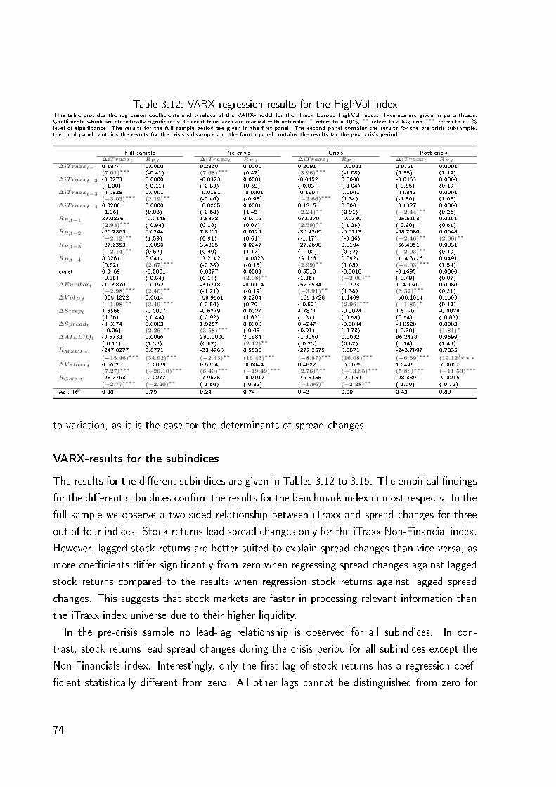
Table 3.12: VARX-regression results for the HighVol indexThis table provides the regression coecients and t-values of the VARX-model for the iTraxx Europe HighVol index. T-values are given in parentheses.Coecients which are statistically signicantly dierent from zero are marked with asterisks. ∗ refers to a 10%, ∗∗ refers to a 5% and ∗∗∗ refers to a 1%level of signicance. The results for the full sample period are given in the rst panel. The second panel contains the results for the pre-crisis subsample,the third panel contains the results for the crisis subsample and the fourth panel contains the results for the post-crisis period.
Full sample Pre-crisis Crisis Post-crisis∆iTraxxt RP,t ∆iTraxxt RP,t ∆iTraxxt RP,t ∆iTraxxt RP,t
∆iTraxxt−1 0.1874 0.0000 0.2860 0.0000 0.2091 -0.0001 0.0725 0.0001(7.01)∗∗∗ (-0.41) (7.68)∗∗∗ (0.47) (3.96)∗∗∗ (-1.08) (1.35) (1.19)
∆iTraxxt−2 -0.0273 0.0000 -0.0323 0.0001 -0.0452 0.0000 -0.0463 0.0000(-1.00) (-0.11) (-0.83) (0.59) (-0.83) (-0.04) (-0.85) (0.19)
∆iTraxxt−3 -0.0838 0.0001 -0.0181 -0.0001 -0.1504 0.0001 -0.0843 0.0001(−3.03)∗∗∗ (2.19)∗∗ (-0.46) (-0.98) (−2.66)∗∗∗ (1.34) (-1.56) (1.08)
∆iTraxxt−4 0.0288 0.0000 -0.0265 0.0001 0.1215 0.0001 -0.1327 0.0000(1.06) (0.88) (-0.68) (1.45) (2.24)∗∗ (0.91) (−2.44)∗∗ (0.26)
RP,t−1 37.0876 -0.0145 1.5378 0.0015 67.0270 -0.0389 -25.5158 0.0161(2.93)∗∗∗ (-0.94) (0.18) (0.07) (2.59)∗∗ (-1.25) (-0.90) (0.51)
RP,t−2 -26.7863 0.0244 7.8001 0.0129 -30.4209 -0.0113 -68.7980 0.0648(−2.12)∗∗ (1.59) (0.91) (0.61) (-1.17) (-0.36) (−2.46)∗∗ (2.06)∗∗
RP,t−3 -27.6353 0.0096 3.4805 0.0247 -27.2698 0.0104 -56.4951 0.0031(−2.14)∗∗ (0.62) (0.40) (1.17) (-1.02) (0.32) (−2.03)∗∗ (0.10)
RP,t−4 8.0267 0.0417 -3.2142 -0.0028 79.1761 0.0527 -114.3776 0.0491(0.62) (2.67)∗∗∗ (-0.38) (-0.13) (2.99)∗∗ (1.65) (−4.03)∗∗∗ (1.54)
const 0.0469 -0.0001 0.0077 0.0003 0.5518 -0.0010 -0.1695 0.0000(0.35) (-0.54) (0.14) (2.08)∗∗ (1.35) (−2.00)∗∗ (-0.49) (0.07)
∆Euribort -19.6870 0.0192 -3.6218 -0.0014 -52.5534 0.0223 114.1309 0.0080(−2.98)∗∗∗ (2.40)∗∗ (-1.21) (-0.19) (−3.91)∗∗ (1.38) (3.32)∗∗∗ (0.21)
∆V olP,t -305.1222 0.6514 -58.9561 0.2284 -165.3728 1.1409 -588.1014 0.1503(−1.98)∗∗ (3.49)∗∗∗ (-0.50) (0.79) (-0.52) (2.96)∗∗∗ (−1.85)∗ (0.42)
∆Steept 1.8566 -0.0007 -0.6279 0.0027 4.7871 -0.0024 1.5120 -0.0028(1.36) (-0.44) (-0.92) (1.63) (1.37) (-0.58) (0.54) (-0.88)
∆Spreadt -0.0074 0.0003 1.9257 0.0000 0.4247 -0.0004 -0.0520 0.0003(-0.06) (2.26)∗∗ (3.58)∗∗∗ (-0.03) (0.91) (-0.78) (-0.30) (1.81)∗
∆AILLIQt -0.5733 0.0086 280.0000 2.1884 -1.8050 0.0082 86.2478 0.9699(-0.11) (1.32) (0.67) (2.12)∗∗ (-0.23) (0.87) (0.14) (1.43)
RMSCI,t -247.0277 0.6771 -33.4760 0.5538 -277.2575 0.6071 -243.7097 0.7835
(−15.46)∗∗∗ (34.92)∗∗∗ (−2.43)∗∗ (16.43)∗∗∗ (−8.87)∗∗∗ (16.08)∗∗∗ (−6.69)∗∗∗ (19.12)∗ ∗ ∗∆V stoxxt 0.6675 -0.0029 0.5834 -0.0044 0.4822 -0.0029 1.2445 -0.0027
(7.27)∗∗∗ (−26.10)∗∗∗ (6.40)∗∗∗ (−19.49)∗∗∗ (2.76)∗∗∗ (−13.85)∗∗∗ (5.88)∗∗∗ (−11.53)∗∗∗
RGold,t -28.7768 -0.0277 -7.9675 -0.0100 -46.3355 -0.0651 -28.8391 -0.0215(−2.77)∗∗∗ (−2.20)∗∗ (-1.60) (-0.82) (−1.96)∗ (−2.28)∗∗ (-1.09) (-0.72)
Adj. R2 0.38 0.79 0.24 0.74 0.43 0.80 0.43 0.80
to variation, as it is the case for the determinants of spread changes.
VARX-results for the subindices
The results for the dierent subindices are given in Tables 3.12 to 3.15. The empirical ndings
for the dierent subindices conrm the results for the benchmark index in most respects. In the
full sample we observe a two-sided relationship between iTraxx and spread changes for three
out of four indices. Stock returns lead spread changes only for the iTraxx Non-Financial index.
However, lagged stock returns are better suited to explain spread changes than vice versa, as
more coecients dier signicantly from zero when regressing spread changes against lagged
stock returns compared to the results when regression stock returns against lagged spread
changes. This suggests that stock markets are faster in processing relevant information than
the iTraxx index universe due to their higher liquidity.
In the pre-crisis sample no lead-lag relationship is observed for all subindices. In con-
trast, stock returns lead spread changes during the crisis period for all subindices except the
Non-Financials index. Interestingly, only the rst lag of stock returns has a regression coef-
cient statistically dierent from zero. All other lags cannot be distinguished from zero for
74

Table 3.13: VARX-regression results for the Senior Financials indexThis table provides the regression coecients and t-values of the VARX-model for the iTraxx Europe Senior Financials index. T-values are given inparentheses. Coecients which are statistically signicantly dierent from zero are marked with asterisks. ∗ refers to a 10%, ∗∗ refers to a 5% and ∗∗∗
refers to a 1% level of signicance. The results for the full sample period are given in the rst panel. The second panel contains the results for the pre-crisissubsample, the third panel contains the results for the crisis subsample and the fourth panel contains the results for the post-crisis period.
Full sample Pre-crisis Crisis Post-crisis∆iTraxxt RP,t ∆iTraxxt RP,t ∆iTraxxt RP,t ∆iTraxxt RP,t
∆iTraxxt−1 0.1588 0.0000 0.2222 0.0000 0.2132 0.0001 0.0601 0.0000(6.11)∗∗∗ (0.17) (6.05)∗∗∗ (0.13) (4.00)∗∗∗ (0.77) (1.16) (-0.58)
∆iTraxxt−2 -0.0949 0.0000 0.0263 0.0002 -0.1063 0.0000 -0.1297 0.0001(−3.61)∗∗∗ (0.91) (0.70) (0.39) (−1.94)∗ (0.23) (−2.62)∗∗∗ (1.77)∗
∆iTraxxt−3 -0.0380 0.0001 0.0191 -0.0003 -0.0415 0.0000 -0.0900 0.0002(-1.41) (2.07∗∗) (0.50) (-0.77) (-0.73) (0.20) (−1.75)∗ (2.30)∗∗
∆iTraxxt−4 -0.1325 0.0000 0.0148 0.0001 -0.0998 0.0001 -0.1446 -0.0001(−4.92)∗∗∗ (-0.08) (0.39) (0.23) (−1.76)∗ (1.04) (−2.82)∗∗∗ (-1.19)
RP,t−1 32.7991 -0.0085 -4.0557 -0.0061 55.3943 -0.0067 6.6538 -0.0249(4.12)∗∗∗ (-0.59) (−2.08)∗∗ (-0.31) (3.51)∗∗∗ (-0.25) (0.33) (-0.77)
RP,t−2 -25.9160 0.0390 1.4735 0.0059 -14.1019 0.0019 -71.9146 0.1069(−3.25)∗∗∗ (2.72)∗∗∗ (0.76) (0.30) (-0.88) (0.07) (−3.84)∗∗∗ (3.50)∗∗∗
RP,t−3 -4.1297 0.0078 -3.7446 0.0311 6.8789 -0.0019 -28.5238 0.0187(-0.51) (0.54) (−1.94)∗ (1.56) (0.42) (-0.07) (-1.50) (0.61)
RP,t−4 -12.6434 0.0321 -1.1761 -0.0165 8.7054 0.0666 -52.0262 0.0070(-1.55) (2.19)∗∗ (-0.61) (-0.83) (0.53) (2.35)∗∗ (−2.70)∗∗∗ (0.22)
const 0.0702 -0.0001 -0.0012 0.0003 0.2372 -0.0010 0.2301 0.0000(0.77) (-0.56) (-0.10) (2.07)∗∗ (0.87) (−2.11)∗∗ (0.97) (-0.04)
∆Euribort -4.7167 0.0182 -0.1676 -0.0013 -16.0948 0.0093 21.4288 0.0273(-1.06) (2.27)∗∗ (-0.23) (-0.17) (−1.76)∗ (0.59) (0.99) (0.78)
∆V olP,t -231.5547 0.6120 6.9056 0.1481 -311.8259 1.6576 -179.9884 -0.0056(−3.69)∗∗∗ (5.42)∗∗∗ (0.25) (0.53) (−1.91)∗ (5.87)∗∗∗ (−1.77)∗ (-0.03)
∆Steept 1.1327 -0.0004 0.0233 0.0030 3.8177 -0.0003 0.5732 -0.0033(1.25) (-0.26) (0.14) (1.80)∗ (1.67)∗ (-0.08) (0.30) (-1.06)
∆Spreadt 0.1408 0.0011 0.1935 -0.0016 0.0713 0.0021 0.3063 0.0003(0.65) (2.87)∗∗∗ (2.06)∗∗ (−1.69)∗ (0.15) (2.55)∗∗ (0.82) (0.56)
∆AILLIQt 4.8699 -0.0109 36.1214 -0.4326 2320.0000 0.0803 4.5440 -0.0117(1.42) (−1.77)∗ (0.59) (-0.69) (1.85)∗ (0.04) (1.05) (−1.66)∗
RMSCI,t -152.5539 0.6750 0.7427 0.5581 -131.3070 0.6051 -207.0969 0.7817(−14.25)∗∗∗ (35.09)∗∗∗ (0.23) (16.53)∗∗∗ (−6.17)∗∗∗ (16.48)∗∗∗ (−8.12)∗∗∗ (18.82)∗∗∗
∆V stoxxt 0.3211 -0.0030 0.1204 -0.0042 0.2068 -0.0031 0.8323 -0.0028(5.13)∗∗∗ (−26.43)∗∗∗ (5.56)∗∗∗ (−19.06)∗∗∗ (1.72)∗ (−15.07)∗∗∗ (5.37)∗∗∗ (−11.00)∗∗∗
RGold,t 1.3125 -0.0333 -2.0667 -0.0061 0.2199 -0.0773 6.0247 -0.0291(0.19) (−2.66)∗∗∗ (−1.75)∗ (-0.50) (0.01) (−2.82)∗∗∗ (0.33) (-0.99)
Adj. R2 0.33 0.79 0.13 0.73 0.30 0.82 0.48 0.80
75
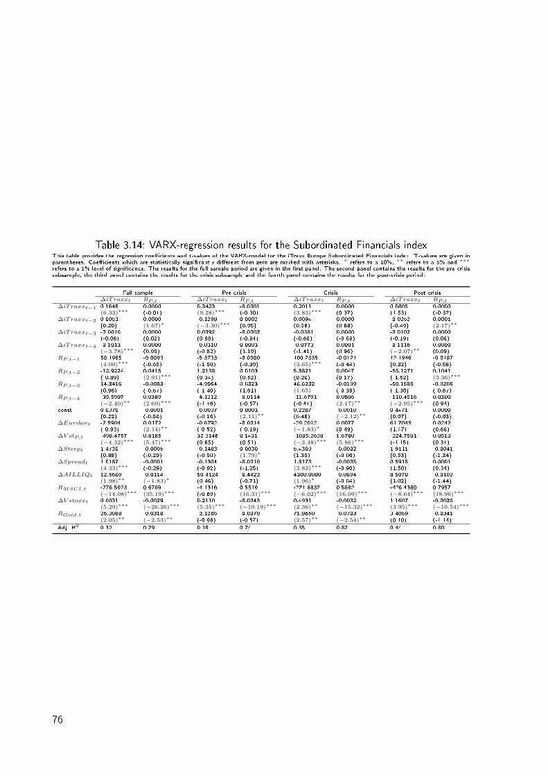
Table 3.14: VARX-regression results for the Subordinated Financials indexThis table provides the regression coecients and t-values of the VARX-model for the iTraxx Europe Subordinated Financials index. T-values are given inparentheses. Coecients which are statistically signicantly dierent from zero are marked with asterisks. ∗ refers to a 10%, ∗∗ refers to a 5% and ∗∗∗
refers to a 1% level of signicance. The results for the full sample period are given in the rst panel. The second panel contains the results for the pre-crisissubsample, the third panel contains the results for the crisis subsample and the fourth panel contains the results for the post-crisis period.
Full sample Pre-crisis Crisis Post-crisis∆iTraxxt RP,t ∆iTraxxt RP,t ∆iTraxxt RP,t ∆iTraxxt RP,t
∆iTraxxt−1 0.1648 0.0000 0.3423 -0.0001 0.2011 0.0000 0.0805 0.0000(6.33)∗∗∗ (-0.01) (9.28)∗∗∗ (-0.30) (3.83)∗∗∗ (0.37) (1.53) (-0.32)
∆iTraxxt−2 0.0053 0.0000 -0.1299 0.0002 0.0094 0.0000 -0.0252 0.0001(0.20) (1.67)∗ (−3.30)∗∗∗ (0.95) (0.18) (0.88) (-0.49) (2.17)∗∗
∆iTraxxt−3 -0.0016 0.0000 0.0392 -0.0002 -0.0381 0.0000 -0.0102 0.0000(-0.06) (0.02) (0.98) (-0.84) (-0.68) (-0.88) (-0.19) (0.08)
∆iTraxxt−4 -0.1013 0.0000 -0.0310 0.0003 -0.0773 0.0001 -0.1116 0.0000(−3.78)∗∗∗ (0.95) (-0.82) (1.19) (-1.41) (0.96) (−2.07)∗∗ (0.09)
RP,t−1 58.1985 -0.0093 -5.3733 -0.0080 100.2335 -0.0121 12.1946 -0.0187(4.00)∗∗∗ (-0.65) (-1.50) (-0.39) (3.65)∗∗∗ (-0.44) (0.32) (-0.58)
RP,t−2 -12.9224 0.0415 1.2138 0.0103 5.5821 0.0047 -55.1271 0.1041(-0.89) (2.91)∗∗∗ (0.34) (0.52) (0.20) (0.17) (-1.52) (3.36)∗∗∗
RP,t−3 14.3416 -0.0083 -4.9964 0.0323 46.6232 -0.0109 -50.1585 -0.0206(0.96) (-0.57) (-1.40) (1.61) (1.65) (-0.39) (-1.38) (-0.67)
RP,t−4 -35.5997 0.0389 -4.1212 -0.0114 -11.6791 0.0606 -110.4516 0.0300(−2.40)∗∗ (2.69)∗∗∗ (-1.16) (-0.57) (-0.41) (2.17)∗∗ (−2.95)∗∗∗ (0.94)
const 0.0370 -0.0001 -0.0037 0.0003 0.2287 -0.0010 0.4471 0.0000(0.22) (-0.56) (-0.16) (2.11)∗∗ (0.48) (−2.12)∗∗ (0.97) (-0.03)
∆Euribort -7.5904 0.0172 -0.6792 -0.0014 -29.2012 0.0077 61.7045 0.0242(-0.93) (2.14)∗∗ (-0.52) (-0.19) (−1.83)∗ (0.49) (1.47) (0.68)
∆V olP,t -498.4757 0.6185 32.2146 0.1431 -1005.2620 1.6760 -224.7501 0.0513(−4.32)∗∗∗ (5.47)∗∗∗ (0.65) (0.51) (−3.48)∗∗∗ (5.86)∗∗∗ (-1.15) (0.31)
∆Steept 1.4730 -0.0005 -0.1483 0.0030 5.4303 -0.0002 1.9111 -0.0041(0.88) (-0.29) (-0.50) (1.79)∗ (1.35) (-0.06) (0.53) (-1.34)
∆Spreadt 1.0187 -0.0001 -0.1304 -0.0010 1.5173 -0.0005 0.5918 0.0001(4.33)∗∗∗ (-0.29) (-0.92) (-1.25) (2.82)∗∗∗ (-0.90) (1.50) (0.34)
∆AILLIQt 12.5600 -0.0114 50.4124 -0.4422 4300.0000 -0.0894 8.5070 -0.0102(1.98)∗∗ (−1.83)∗ (0.46) (-0.71) (1.96)∗ (-0.04) (1.02) (-1.44)
RMSCI,t -276.5923 0.6769 -4.1316 0.5519 -221.8832 0.5882 -426.4380 0.7957(−14.08)∗∗∗ (35.19)∗∗∗ (-0.69) (16.31)∗∗∗ (−6.02)∗∗∗ (16.09)∗∗∗ (−8.64)∗∗∗ (18.96)∗∗∗
∆V stoxxt 0.6031 -0.0029 0.2110 -0.0043 0.4931 -0.0032 1.1607 -0.0026(5.29)∗∗∗ (−26.26)∗∗∗ (5.35)∗∗∗ (−19.19)∗∗∗ (2.36)∗∗ (−15.32)∗∗∗ (3.95)∗∗∗ (−10.54)∗∗∗
RGold,t 26.3088 -0.0318 -2.1285 -0.0070 71.9650 -0.0703 3.4059 -0.0341(2.05)∗∗ (−2.53)∗∗ (-0.98) (-0.57) (2.57)∗∗ (−2.54)∗∗ (0.10) (-1.14)
Adj. R2 0.32 0.79 0.19 0.74 0.35 0.82 0.44 0.80
76
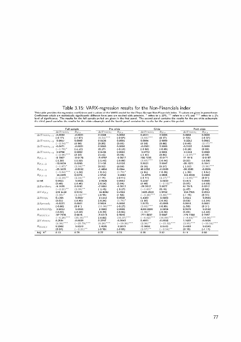
Table 3.15: VARX-regression results for the Non-Financials indexThis table provides the regression coecients and t-values of the VARX-model for the iTraxx Europe Non-Financials index. T-values are given in parentheses.Coecients which are statistically signicantly dierent from zero are marked with asterisks. ∗ refers to a 10%, ∗∗ refers to a 5% and ∗∗∗ refers to a 1%level of signicance. The results for the full sample period are given in the rst panel. The second panel contains the results for the pre-crisis subsample,the third panel contains the results for the crisis subsample and the fourth panel contains the results for the post-crisis period.
Full sample Pre-crisis Crisis Post-crisis∆iTraxxt RP,t ∆iTraxxt RP,t ∆iTraxxt RP,t ∆iTraxxt RP,t
∆iTraxxt−1 -0.0030 -0.0001 0.2229 0.0000 0.2011 0.0000 0.0805 0.0000(-0.12) (-1.62) (6.54)∗∗∗ (-0.02) (3.83)∗∗∗ (0.37) (1.53) (-0.32)
∆iTraxxt−2 -0.0657 0.0000 0.0136 0.0001 0.0094 0.0000 -0.0252 0.0001(−2.54)∗∗ (0.98) (0.39) (0.65) (0.18) (0.88) (-0.49) (2.17)∗∗
∆iTraxxt−3 -0.0471 -0.0001 0.0060 0.0000 -0.0381 0.0000 -0.0102 0.0000(−1.79)∗ (-1.12) (0.17) (-0.14) (-0.68) (-0.88) (-0.19) (0.08)
∆iTraxxt−4 -0.0766 0.0000 0.0498 0.0002 -0.0773 0.0001 -0.1116 0.0000(−2.98)∗∗∗ (0.23) (1.46) (0.93) (-1.41) (0.96) (−2.07)∗∗ (0.09)
RP,t−1 -8.3902 -0.0128 -5.9762 -0.0017 100.2335 -0.0121 12.1946 -0.0187(-1.30) (-1.03) (-1.46) (-0.08) (3.65)∗∗∗ (-0.44) (0.32) (-0.58)
RP,t−2 -12.0634 0.0293 2.1438 0.0120 5.5821 0.0047 -55.1271 0.1041(−1.87)∗ (2.34)∗∗ (0.53) (0.59) (0.20) (0.17) (-1.52) (3.36)∗∗∗
RP,t−3 -25.1629 -0.0162 -1.4866 0.0344 46.6232 -0.0109 -50.1585 -0.0206(−3.84)∗∗∗ (-1.28) (-0.37) (1.70)∗ (1.65) (-0.39) (-1.38) (-0.67)
RP,t−4 -14.3395 0.0274 4.5720 -0.0082 -11.6791 0.0606 -110.4516 0.0300(−2.19)∗∗ (2.16)∗∗ (1.14) (-0.41) (-0.41) (2.17)∗∗ (−2.95)∗∗∗ (0.94)
const 0.0411 -0.0001 -0.0038 0.0003 0.2287 -0.0010 0.4471 0.0000(0.48) (-0.46) (-0.14) (2.04) (0.48) (−2.12)∗∗ (0.97) (-0.03)
∆Euribort -9.1635 0.0192 -2.0861 -0.0012 -29.2012 0.0077 61.7045 0.0242(−2.21)∗∗ (2.39)∗∗ (-1.40) (-0.17) (−1.83)∗ (0.49) (1.47) (0.68)
∆V olP,t 226.3420 0.9222 -34.6043 0.4903 -1005.2620 1.6760 -224.7501 0.0513(1.95)∗ (4.10)∗∗∗ (-0.55) (1.56) (−3.48)∗∗∗ (5.86)∗∗∗ (-1.15) (0.31)
∆Steept 0.4305 -0.0007 -0.1152 0.0030 5.4303 -0.0002 1.9111 -0.0041(0.51) (-0.45) (-0.34) (1.76)∗ (1.35) (-0.06) (0.53) (-1.34)
∆Spreadt -0.0223 0.0001 0.5624 0.0000 1.5173 -0.0005 0.5918 0.0001(-0.66) (0.84) (11.96)∗∗∗ (-0.17) (2.82)∗∗∗ (-0.90) (1.50) (0.34)
∆AILLIQt -0.0033 -0.0001 -0.0082 0.0000 4300.0000 -0.0894 8.5070 -0.0102(-0.02) (-0.18) (-0.20) (-0.06) (1.96)∗ (-0.04) (1.02) (-1.44)
RMSCI,t -62.7936 0.6815 -5.6313 0.5540 -221.8832 0.5882 -426.4380 0.7957(−6.28)∗∗∗ (35.16)∗∗∗ (-0.83) (16.37)∗∗∗ (−6.02)∗∗∗ (16.09)∗∗∗ (−8.64)∗∗∗ (18.96)∗∗∗
∆V stoxxt 0.2534 -0.0029 0.2797 -0.0043 0.4931 -0.0032 1.1607 -0.0026(4.36)∗∗∗ (−25.79)∗∗∗ (6.26)∗∗∗ (−19.30)∗∗∗ (2.36)∗∗ (−15.32)∗∗∗ (3.95)∗∗∗ (−10.54)∗∗∗
RGold,t 0.2902 -0.0279 -1.4285 -0.0079 71.9650 -0.0703 3.4059 -0.0341(0.04) (−2.21)∗∗ (-0.58) (-0.65) (2.57)∗∗ (−2.54)∗∗ (0.10) (-1.14)
Adj. R2 0.13 0.79 0.27 0.73 0.35 0.82 0.44 0.80
77
all subindices. This can be interpreted as a sign that investors are especially sensitive to new
information in times of crises and therefore incorporate new information promptly.
In the post-crisis period we observe a two-sided relationship for all subindices except for the
HighVol index, where stock returns lead spread changes. For the Senior Financials and the
Subordinated Financials index, the predictive power of lagged spread changes when regressed
against stock returns is equal to the predictive power when regressing spread changes against
lagged stock returns or even slightly higher. The lead-lag relationship has shifted in favor
of lagged spread changes in the aftermath of the crisis. This is true for all but one index,
and most pronounced for the two nancial indices. As the nancial sector is widely believed
to contribute signicantly to systemic risk, this actually leads us to the conclusion that the
iTraxx index contains useful information regarding systemic risk that is actually incorporated
by market participants.
Again, there is empirical evidence that there is variation in the lead-lag relationship between
the market for credit risk an stock markets. While stock returns lead spread changes in the
crisis period, no apparent lead-lag relationship between the two can be observed in the pre-
crisis period. In the post crisis period we observe a two-sided relationship between the two
markets. In general, the results suggest that the role of credit markets in processing rm
specic information has strengthened through time. Thus, systemic risk measured in credit
markets is priced in equity markets and it is necessary to rely on information from both markets
when one engages in trading or hedging.
3.7 Conclusion
This paper empirically investigates the behavior of iTraxx Europe spread changes around the
2007-2009 nancial crisis. The iTraxx index universe is of special interest, as iTraxx spreads
can be interpreted as a measure of systemic risk. We examine the determinants of iTraxx
spread changes, as well as changes in these determinants due to the recent nancial crisis. We
nd empirical evidence that iTraxx spread change determinants are subject to variation in the
course of the nancial crisis. While stock returns and implied stock market volatility explain
most of the variation in the post crisis period, global variables have a statistically signicant
inuence in the pre-crisis and crisis period. In general the explanatory power of our set of
independent variables is increasing throughout the sample.
In order to check for the robustness of the regression results we perform a quantile regression.
This approach allows us to assess the explanatory power of our set of independent variable
for spread changes in the upper and lower tail of the empirical distribution. We nd empirical
78

evidence that a signicant systematic fraction of spread changes in the tails of the empirical
distribution is not explained by the independent variables, suggesting that additional factors
have to be incorporated when explaining large spread widenings or large spread tightenings
that are not implied by structural models.
We additionally investigate changes in the lead-lag relationship between iTraxx spread
changes and stock returns during the recent nancial crisis in order to assess whether market
participants rely on the iTraxx index universe as a source of information regarding systemic risk.
We nd empirical evidence that the lead-lag relationship is subject to variation as well. While
stock returns lead spread changes in the crisis period, a two-sided relationship is observed in
the post crisis period.
Our results provide further insights in the mechanics of credit markets. Future research
might focus on the modeling of iTraxx spread changes in the upper and lower tail of the
empirical distributions, since standard models fail to explain large spread changes. Another
interesting approach is whether changes in factor sensitivities of spreads can be observed before
a market turmoil evolves, i.e. whether factor sensitivities can be used as a warning signal in
nancial markets.
79

Bibliography
Alexander, Carol and Andreas Kaeck (2008): Regime dependent determinants of credit default
swap spreads, Journal of Banking & Finance 32: 10081021.
Amihud, Yakov (2002): Illiquidity and stock returns: Cross-section and time-series eects,
Journal of Financial Markets 5: 3156.
Benkert, Christoph (2004): Explaining credit default swap premia, Journal of Futures Markets
24: 7192.
Berndt, Antje, Rohan Douglas, Darrell Due, Mark Ferguson, and David Schranz (2005):
Measuring default risk premia from default swap rates and EDFs, Working Paper 173, Bank
for International Settlements.
Byström, Hans (2005): Credit default swaps and equity prices: The iTraxx CDS index market,
Working paper, Lund University.
Campbell, John and Glen Taksler (2002): Equity volatility and corporate bond yields, Working
paper, Harvard - Institute of Economic Research.
Chow, Greogory (1960): Tests of equality between sets of coecients in two linear regressions,
Econometrica 28: 591605.
Collin-Dufresne, Pierre, Robert Goldstein, and J. Martin (2001): The determinants of credit
spread changes, Journal of Finance 56: 21772207.
Das, Sanjiv R. and Paul Hanouna (2009): Hedging credit: Equity liquidity matters, Journal of
Financial Intermediation 18: 112123.
Due, Darrel and Kenneth Singleton (2003): Credit Risk: Pricing Measurement and Man-
agement (Princeton University Press, Princeton).
Due, Darrell, Leandro Saita, and Ke Wang (2007): Multi-period corporate default prediction
with stochastic covariates, Journal of Financial Economics 83: 635665.
Due, Darrell and Kenneth Singleton (1999): Modeling term structures of defaultable bonds,
Review of Financial Studies 12: 687720.
Ericsson, Jan, Kris Jacobs, and Rodolfo Oviedo-Helfenberger (2004): The determinants of
credit default swap premia, Working paper, Swedish Institute for Financial Research.
80
Fung, Hung-Gay, Gregory Sierra, Jot Yau, and Zhang Gaiyan (2008): Are the U.S. stock
market and credit default swap market related? Evidence from the CDX indices, Working
paper, University of MissouriSt. Louis.
Giammarino, Flavia and Pauline Barrieu (2009): A semiparametric model for the systematic
factors of portfolio credit risk premia, Journal of Empirical Finance 16: 655670.
Hannan, Edward and Barry Quinn (1979): The determination of the order of an autoregression,
Journal of the Royal Statistical Society. Series B (Methodological) 41: 190195.
Jarrow, Robert, David Lando, and Stuart Turnbull (1997): A markov model for the term
structure of credit risk spreads, Review of Financial Studies 10: 481523.
Koenker, Roger and Gilbert Jr. Bassett (1978): Regression quantiles, Econometrica 46(1):
3350.
Koenker, Roger and Kevin F. Hallock (2001): Quantile regression, Journal of Economic Per-
spectives 15: 143156.
Lando, David (1998): On cox processes and credit risky securities, Review of Derivatives
Research 2: 99120.
Longsta, Francis and Arvind Rajan (2008): An empirical analysis of the pricing of collateral-
ized debt obligations, Journal of Finance 63: 529563.
Markit (2010a): Markit credit indices: A primer, Technical report, Markit Group.
Markit (2010b): Markit iTraxx indices: Index level calculation, Technical report, Markit Group.
Markit (2011): Markit iTraxx Europe: Index rules, Technical report, Markit Group.
Merton, Robert (1974): On the pricing of corporate debt: The risk structure of interest rates,
Journal of Finance 29: 449470.
Norden, Lars and Martin Weber (2009): The co-movement of credit default swap, bond and
stock markets: An empirical analysis, European Financial Management 15: 529562.
Pan, Jun and Kenneth Singleton (2005): Default and recovery implicit in the term structure
of sovereign CDS spreads, Working paper, MIT and Stanford.
Scheicher, Martin (2008): How has CDO market pricing changed during the turmoil?, Working
paper, European Central Bank.
81

Tang, Dragon and Hong Yan (2007): Liquidity and credit default swap spreads, Working
paper, University of Hong Kong.
82

4 The Method of Maximum Implied
Default Correlation and its
Potential Applications
The Method of Maximum Implied Default Correlation
and its Potential Applications
Bastian Breitenfellner
2012
Abstract
Default dependence is of paramount importance when portfolio products or credit derivatives
subject to counterparty risk have to be evaluated. Unfortunately, the modeling of default
dependence is non-trivial and very sensitive to the underlying assumptions. In this light, a
method that makes it possible to estimate the potential inuence of default dependence on a
certain nancial instrument is desirable. I introduce the method of maximum implied default
correlation as a potential solution to this problem. It is based on market-implied pairwise
bounds for the default correlation of the entities under consideration. I apply the method
to default swaps subject to counterparty risk and basket credit derivatives to illustrate the
potential inuence of default correlation on the respective spreads. I show that the potential
inuence of assumptions concerning default correlation is especially large for homogeneous
portfolios with investment grade issuers. In general, the bounds for spreads implied by the
method of maximum implied default correlation are wide, in particular for portfolio products,
limiting its practical relevance as a pricing tool. However, although the method seems to have
limited practical relevance as a pricing tool, it is well suited to asses the potential inuence of
assumptions concerning default correlation on nancial securities sensitive to default depen-
dence and as a tool for stress testing.
Keywords: default correlation, counterparty risk, credit derivatives, credit risk
84
4.1 Introduction
The pricing of securities subject to credit risk has gained major attention within nancial market
research in recent years. Usually, this task involves deriving the distribution of default times of
the entities under consideration. In case that securities subject to counterparty risk or portfolio
products have to be priced, joint distributions of default times have to be estimated. If default
times are dependent, i.e. if defaults are correlated, this becomes a complex task. Furthermore,
the results obtained are highly sensitive to assumptions concerning the dependence structure
of the entities' default times.
During the recent nancial crisis many of the assumptions behind standard pricing models
for portfolio products proved to be myopic. Approaches such as the Gaussian copula, which
is applied in latent variable models, do not account for extreme default dependence, i.e. the
clustering of defaults. However, this clustering is a common feature of distressed nancial
markets and was also observed during the recent nancial crisis. Therefore, the market's per-
ception concerning the inherent risks of portfolio products were not adequate, as common
models of dependent defaults are highly sensitive with respect to assumptions regarding the
dependence structure (Frey and McNeil (2003)). Models allowing for extreme (possibly asym-
metric) dependence of default times are available. However, they are complex and dicult to
implement. In this light there is a pronounced need for concepts allowing to stress test prices
of portfolio products, possibly leading to bounds within the prices (spreads) of such products
have to lie in between in the absence of arbitrage opportunities and that hold regardless of the
actual dependence structures within the portfolio members. Such concepts allow for a decent
understanding of the inherent risk of portfolio products as they provide insights concerning
the impact of default correlation on the pricing of these products. Hence, market participants
can assess in which range changes in the assumptions concerning the dependence structure of
entities within the portfolio do aect the fair prices of these securities.
This paper addresses the problem outlined above by introducing the method of maximum
implied default correlation. It contributes to the existing literature by deriving upper and lower
bounds for the default correlation for pairs of entities using market data. These bounds hold
as long as no arbitrage opportunities exist. These bounds in turn can be used to derive upper
and lower bounds for the prices of securities that are subject to credit risk and sensitive to
default correlation. Examples of such securities are credit default swaps (CDS) subject to
counterparty risk and nth-to-default baskets.
I apply the method of maximum implied default correlation to derive bounds for the prices of
these two securities using an intuitive and easy to implement Monte Carlo simulation algorithm,
which is based on an simple intensity model of default. The algorithm involves several steps.
85

First, implied upper bounds for the default correlation of certain entities are calculated based
on observed market data. Next, the implied upper default correlations are converted into a
variance-covariance matrix of the respective default processes. In a succeeding step I model
the default processes relying on the overlapping sums (OS) method. This involves expressing
the default process of each entity under consideration as a sum of independent idiosyncratic
as well as common default processes. For each entity its respective sum of default processes
is calibrated to match the respective implied variance-covariance matrix of its default process.
This is achieved by applying the algorithm of Park and Shin (1998).1 Consequently, the default
times of each entity under consideration are simulated, allowing to derive the upper bound
for securities with sensitivity to the default of the entity under consideration. The respective
lower bound can be simulated by assuming that defaults are independent, i.e. that no default
correlation is present. In addition to calculating upper and lower bounds for nth-to-default
baskets and CDS subject to counterparty risk, I analyze the sensitivity of the respective spreads
concerning changes in the correlation structure of the underlying entities to provide a better
understanding of the potential impact of default correlation.
The proposed approach allows for the comparison of market spreads for credit derivatives
with model-implied maximum and minimum spreads, without extensive modeling of default
correlations. In the absence of arbitrage opportunities, market quotes have to lie in between
the implied bounds, regardless of the underlying default correlation structure between the
entities contributing to the risk of the security under consideration. Hence, this paper provides
further insights on the impact of default correlation on spreads of credit derivatives sensitive
to default correlation and the eciency of the credit derivatives market as a whole.
The remainder of this paper is organized es follows. In Section 4.2 I provide an overview of
models for pricing credit derivatives such as CDS and introduce the intensity model on which
the Monte Carlo simulations are based. In Section 4.3 I discuss the concept of default correla-
tion and show how upper and lower bounds for the default correlation between two issuers can
be implied from market data. The issue of simulating an intensity model incorporating default
correlation is addressed in Section 4.4. Section 4.5 presents the results of the simulations. In
Section 4.6 i present an alternative application for the method of maximum implied default
correlation. Section 4.7 concludes the paper.
1An example how the algorithm works is provided in the appendix.
86
4.2 Related Literature
There are two major classes of models for dependent defaults. The rst class comprises ex-
tensions of the Merton (1974) structural model. In this class of models, default occurs if a
latent variable, usually interpreted as the asset value of the obligor, hits a certain threshold.
Dependence between the defaults of multiple issuers is introduced via dependent latent vari-
ables, e.g. correlated asset value processes. Examples for this class of models are the Moody's
KMV Model or RiskMetrics. The second class of models consists of so called mixture mod-
els. In this class of models the default probability of an obligor is expressed as a function
of certain, possibly economic, factors. Default dependence is introduced if certain obligors
are exposed to similar factors. Conditioning on the factors, defaults of the single obligors are
independent. The CreditRisk+ model is an example of this class of models. According to Frey
and McNeil (2003) both approaches share the feature that they are highly sensitive to the
assumptions regarding the dependence structure between dierent obligors. Mixture models
can be combined with the class of intensity models in the spirit of Jarrow and Turnbull (1995).
This approach has e.g. been applied by Due and Gârleanu (2001). In intensity models,
default is an unpredictable event governed by the rst jump of a Poisson process. The default
probability depends on the respective hazard rate. In this class of models default dependence
can be introduced by correlating the hazard rate processes of dierent entities. However, as
stated by Jarrow and Yu (2001), the default correlation attainable in this class of models is
low unless one allows for large jumps in the default intensities of the surviving entities in case
of an observed default.
For the pricing of securities subject to credit risk, default dependence plays a role in two
distinct ways. One the one hand, default correlation has to be incorporated when portfolio
products, such as collateralized debt obligations (CDO) and nth-to-default swaps, have to be
priced. In both cases the cash ows of the security depend on the solvency of a portfolio of
entities. In case of pronounced default dependence within the portfolio, a clustering of defaults
is possible, i.e. multiple portfolio constituents default almost simultaneously before the security
matures. Several papers address the pricing of portfolio products. Due and Gârleanu (2001),
Longsta and Rajan (2008) and Giesecke and Kim (2011) rely on an intensity framework to
evaluate CDO tranches. Hull and White (2004) and Laurent and Gregory (2005) price CDO
and nth-to-default swaps relying on a mixture model with dierent copula assumptions. Li
(2000) relies on a latent variable model with applications to single name CDSs and rst-to-
default swaps. Jabbour et al. (2009) evaluates nth-to-default swaps with default dependence
governed by Gaussian and Student-t copulas.
On the other hand, default correlation is an issue when credit derivatives subject to counter-
87
party risk, such as over-the-counter (OTC) CDS, have to be evaluated. As credit derivatives
are often OTC products, introducing the concept of counterparty risk is a natural expansion to
the problem of pricing such derivatives. The presence of counterparty risk in CDS markets is
conrmed by Jorion and Zhang (2008), who nd signicant empirical evidence that counter-
party risk is an important driver of CDS spreads. The issue of pricing credit derivatives subject
to counterparty risk has been addressed in numerous papers. Hull and White (2001) rely
on a structural framework, while Jarrow and Yu (2001) and Leung and Kwok (2005) employ
an intensity model to price credit risky securities subject to counterparty risk such as CDSs.
Mashal and Naldi (2005) introduce the concept of bounds for credit derivatives. They derive
upper and lower bounds for swap spreads subject to counterparty risk. Furthermore, Turnbull
(2005) adds to the aforementioned approach and derives upper and lower bounds for prots
and losses due to such default swaps. However, as opposed to the approach proposed in this
paper, these bounds do not hold regardless of the assumptions made concerning the default
correlation between the dierent entities involved.
4.3 Correlated Defaults and Implied Bounds for
Default Correlation
Correlated defaults contribute signicantly to credit risk. Default correlation refers to the case
when the default process of an entity is related to the default process of another or several
other entities. There are several potential sources of default correlation, with some examples
discussed below:
• Several entities are exposed to common systematic factors,
• entities have direct exposures with other entities,
• unhedged protection selling and default of the reference entity,
• regulatory capital requirements due to positions in the CDS market which are hedged
via osetting positions written by a distressed entity.
An exposure to common systematic factors is an obvious reason for default correlation. This is
the case when entities are engaged in the same region, or in the same industry. If the industry
faces a demand shock, all entities will be negatively aected, although to dierent degrees.
Some of the entities in the industry might not survive the shock and hence, their defaults are
correlated due to the common exposure to the demand shock. A direct involvement between
88
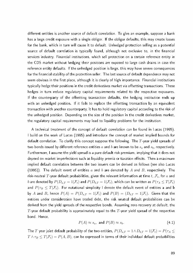
dierent entities is another source of default correlation. To give an example, suppose a bank
has a large credit exposure with a single obligor. If the obligor defaults, this may create losses
for the bank, which in turn will cause it to default. Unhedged protection selling as a potential
source of default correlation is typically found, although not exclusive to, in the nancial
services industry. Financial institutions, which sell protection on a certain reference entity in
the CDS market without hedging their positions are exposed to large cash drains in case the
reference entity defaults. If the unhedged position is large, this may have severe consequences
for the nancial stability of the protection seller. The last source of default dependence may not
seem obvious in the rst place, although it is clearly of high importance. Financial institutions
typically hedge their positions in the credit derivatives market via osetting transactions. These
hedges in turn reduce regulatory capital requirements related to the respective exposures.
If the counterparty of the osetting transaction defaults, the hedging institution ends up
with an unhedged position. If it fails to replace the osetting transaction by an equivalent
transaction with another counterparty, it has to hold regulatory capital according to the risk of
the unhedged position. Depending on the size of the position in the credit derivatives market,
the regulatory capital requirements may lead to liquidity problems for the institution.
A technical treatment of the concept of default correlation can be found in Lucas (1995).
I build on the work of Lucas (1995) and introduce the concept of market implied bounds for
default correlation. To clarify this concept suppose the following. The T -year yield spreads of
two bonds issued by dierent reference entities a and b are known to be sa and sb, respectively.
Furthermore, I assume the yield spread is a pure default risk premium, implying that it does not
depend on market imperfections such as liquidity premia or taxation eects. Then a maximum
implied default correlation between the two issuers can be derived as follows (see also Lucas
(1995)). The default event of entities a and b are denoted by A and B, respectively. The
risk-neutral T -year default probabilities, given the relevant information at time t, Ft, for a andb are denoted by P (Da,T = 1|Ft) and P (Db,T = 1|Ft), which can be written as P (τA ≤ T |Ft)and P (τB ≤ T |Ft). For notational simplicity I denote the default event of entities a and b
by A and B, hence P (A) = P (Da,T = 1|Ft) and P (B) = (Db,T = 1|Ft). Given that the
entities under consideration have traded debt, the risk neutral default probabilities can be
derived from the yield spreads of the respective bonds. Assuming zero recovery at default, the
T -year default probability is approximately equal to the T -year yield spread of the respective
bond. Hence,
P (A) ≈ sa, and P (B) ≈ sb. (4.1)
The T -year joint default probability of the two entities, P (Da,T = 1∧Db,T = 1|Ft) = P (τA ≤T ∧ τB ≤ T |Ft) = P (A,B), can be expressed in terms of their individual default probabilities
89

and their T -year default correlation ρA,B, i.e.
P (A,B) = P (A)P (B) + ρA,B√P (A)(1− P (A))
√P (B)(1− P (B)), (4.2)
where
ρA,B =σA,BσAσB
,
σA =√P (A)(1− P (A)), σB =
√P (B)(1− P (B)),
and
σA,B = E(AB)− E(A)E(B).
As the joint default probability is unobservable, the default correlation between entity a and b
cannot be derived from equation (4.2). Nevertheless, market yield spreads of the two entities
can be used to imply upper and lower bounds for the joint default probability, which in turn can
be used to derive upper and lower bounds for the default correlation between the two entities.
This is because the maximum joint default probability of the two entities cannot exceed the
lower of the two individual default probabilities, whereas the minimum joint default probability
is zero, implying that defaults of the reference entities are mutually exclusive events. Hence,
for the joint default probability P (A,B),
0 ≤ P (A,B) ≤ min[P (A), P (B)] (4.3)
must hold.
Substituting equation (4.3) into equation (4.2) and rearranging terms leaves us with upper
and lower bounds for the default correlation between default events A and B, i.e.
ρA,B ≥−P (A)P (B)√
P (A)(1− P (A))√P (B)(1− P (B))
, (4.4)
and
ρA,B ≤min[P (A), P (B)]− P (A)P (B)√P (A)(1− P (A))
√P (B)(1− P (B))
. (4.5)
From inequalities (4.4) and (4.5) we see that the maximum, as well as the minimum implied
default correlation between two issuers is a function of the individual default probabilities as
well as the maximum attainable joint default probability of the two reference entities. Figure
4.1 illustrates the maximum attainable default correlation as a function of the spread between
the individual default probabilities and the maximum joint default probability. We see that
the maximum attainable default correlation is positively related to the maximum joint default
90
probability and negatively related to the spread between the individual default probabilities of
the two entity under consideration.
Figure 4.1: Maximum attainable implied default correlation as a function of the spread betweenindividual default probabilities and maximum attainable joint default probability
0
0.00
25
0.01
0.02
0.03
0.04
0.05
0.06
0.07
0.08
0.09
0.1
0.00125
0.015
0.035
0.055
0.075
0.095
0
0.2
0.4
0.6
0.8
1
Max
imu
m d
efau
lt c
orr
elat
ion
Spread
Maximum joint default probability
4.4 Incorporating Default Correlation into an
Intensity-Based Pricing Framework for Credit
Derivatives
When it comes to the pricing of securities subject to credit risk, default correlation is of
particular importance if the payments the security promises are contingent to the solvency
of more than one entity. This is for example the case with credit derivatives subject to
counterparty risk or securities with payos contingent on the solvency of a portfolio of entities.
In this case we have to explicitly incorporate the dependence structure between the default
times of the single entities.
Intensity models are commonly used to price securities subject to credit risk. One possible
way to incorporate default correlation between dierent entities into an intensity-based model
91
is by allowing for correlated intensity processes. Nevertheless, as discussed in Hull and White
(2001), the magnitude of default correlation attainable by means of correlated default intensi-
ties is low, even if the processes are perfectly correlated. One way to overcome this problem,
is to allow for large jumps in the default intensity of one entity, if a related entity defaults, as
proposed by Jarrow and Yu (2001).
In this paper I rely on an alternative way to incorporate default correlation in an intensity-
based pricing framework, the overlapping sums (OS) method. The OS method is discussed in
Holgate (1964), among others. The method has been applied by Madsen and Dalthorp (2007)
to simulate correlated count data. The idea behind the OS method is to split the default
processes of the entities under consideration into idiosyncratic and common components. To
illustrate this concept, suppose we are interested in generating correlated Poisson variables
A and B with intensity λA, λB and covariance σA,B, i.e. the default processes of entities a
and b. Suppose that the Poisson variables are constructed as a sum of independent Poisson
variables X, Y, and Z, such that
A = X + Y
and
B = X + Z.
Although X, Y and Z are independent, the processes A and B are correlated via the com-
mon component X. The covariance between the two sums is governed by the overlapping
component, i.e.
σA,B = λX ,
where λX denotes the intensity of the process X. This method can be easily adapted to
the method of maximum implied default correlation described in Section 4.3 by modeling the
default process of each entity under consideration as a sum of overlapping default processes
that yields the desired dependence structure. An example is provided in the appendix.
Using the OS method to model the default process has some intuitive implications. The
default process for each entity is split into an idiosyncratic component, the non-overlapping
Poisson process and a common, or correlation component, the overlapping Poisson process.
Hence, there are two possible reasons for a specic entity to default. Default can be triggered by
the idiosyncratic component, representing a default due to rm specic reasons. Additionally,
an entity can default due to contagion eects. These contagion eects may represent inter-
rm relations between two entities, or a systemic component, where the default of a major
player within a certain industry has negative eect for the nancial stability of other members
of the industry.
92
Due to the nature of the OS method, rms defaulting as a consequence of contagion default
simultaneously. In this case there is no lag between their respective default times, as it would
be likely in the real world. In order to model lagged dependent defaults, a model like the
one of Jarrow and Yu (2001) needs to be applied, where the default of an entity may cause
jumps in the default intensities of its counterparties. Nevertheless, for the evaluation of a
CDS, a lagged dependent default has no inuence on expected payos due to the default of
the reference entity, as long as we assume immediate settlement of the contract as soon as
a credit event occurs. In case portfolio products are under consideration, the simultaneous
defaults become an issue. For my purpose this feature of the OS method is actually desirable,
as I am interested in deriving bounds for the spreads of these securities, and simultaneous
defaults are helpful for describing the worst case scenario.
The OS method is used in the remainder of this paper to generate dependent default times
and examine the eect of default correlation on the prices of securities sensitive to default
dependence via Monte Carlo simulation.2 One drawback of the OS method is that negative
default correlations cannot be attained. However, this is not critical for deriving upper and
lower bounds for CDS prices, as long as we assume that the CDS contract is immediately
closed after one of the three involved parties defaults. In other words, for protection payment
counterparty risk is only an issue, if defaults happen simultaneously. In this case, two special
cases are of interest. In the rst one, the protection seller and the reference entity default
simultaneously, in which case the protection buyer is not compensated for his losses. In
the second one, the protection buyer and the reference entity default simultaneously, and
accordingly the protection seller does not have to compensate the protection buyer. What
happens after the rst credit event, be it a correlated or a single entity default, is of no
relevance for the pricing of the CDS at hand, and therefore negative default correlations do
not have to be accounted for.
When credit derivatives with payos depending on the default processes of a portfolio of
entities are considered, negative default correlation matters. However, the (downside) risk of
the portfolio is clearly determined by positive default correlation. Additionally, there are few
cases where pronounced negative default correlation is observed in reality. Therefore, I do not
consider negative default correlation when simulating the implied bounds for these securities.
2Alternative approaches to simulate dependent default times are discussed in Due and Singelton (1999),Joshi and Kainth (2004), Chen and Glasserman (2008) and Giesecke et al. (2011) among others.
93

4.5 Possible Applications for the Method of Maximum
Implied Default Correlation
4.5.1 General Methodology
For the simulation analysis I rely on the reduced form pricing framework. Therefore, I suppose
that the uncertainty within the economy during the time horizon T can be described by the
ltered probability space (Ω, F , FtTt=0, P ), where F = FT , and P is the equivalent martin-
gale measure under which discounted security prices are martingales. I assume the uniqueness
and existence of P , hence security markets are priced by arbitrage as shown by Harrison and
Kreps (1979) in a discrete time setting and Harrison and Pliska (1981) in continuous time.
The default time of entity i is dened as
τi = inf
t :
∫ t
0
λi,s ds ≥ ξi
, (4.6)
where ξi, i = 1, ..., N is a set of independent unit mean exponential random variables. The
intensity λi,t is predictable under Ft and has right-continuous sample paths. Therefore, the
default time of entity i conditional on the information set Ft is given by the distribution
function
P (τi > t|Ft) = exp
(−∫ t
0
λi,s ds
), t ∈ [0, T ],
and the default process of entity i is dened as
Di,t = 1τi≤t.
The process governing the default intensity λi,t can be modeled in various ways. Lando (1998),
for instance, models the default intensity as a double stochastic Poisson process (Cox process),
driven by set of economic state variables. These state variables are governed by an Rd-valued
state process Xt, where d is the number of the state variables governing the intensity process.
In case default correlation is present λi,t also depends on the default processes of other entities.
Hence, the ltration Ft is generated jointly by the state variables and the default processes,
i.e.
Ft = FX,t ∨ F1,t ∨ ... ∨ FN,t,
where
FX,t = σXs, 0 ≤ s ≤ t and Fi,t = σDi,s, 0 ≤ s ≤ t
represent the ltrations generated by the the processes Xt and Di,t, respectively.
94
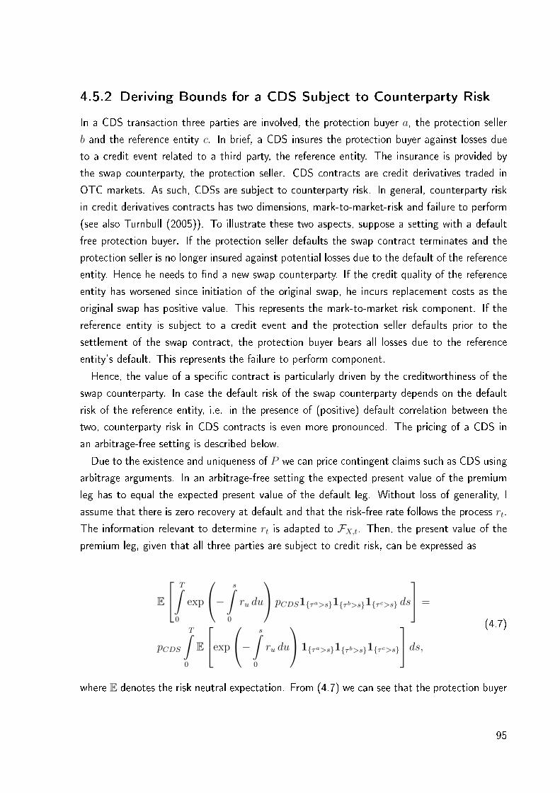
4.5.2 Deriving Bounds for a CDS Subject to Counterparty Risk
In a CDS transaction three parties are involved, the protection buyer a, the protection seller
b and the reference entity c. In brief, a CDS insures the protection buyer against losses due
to a credit event related to a third party, the reference entity. The insurance is provided by
the swap counterparty, the protection seller. CDS contracts are credit derivatives traded in
OTC markets. As such, CDSs are subject to counterparty risk. In general, counterparty risk
in credit derivatives contracts has two dimensions, mark-to-market-risk and failure to perform
(see also Turnbull (2005)). To illustrate these two aspects, suppose a setting with a default
free protection buyer. If the protection seller defaults the swap contract terminates and the
protection seller is no longer insured against potential losses due to the default of the reference
entity. Hence he needs to nd a new swap counterparty. If the credit quality of the reference
entity has worsened since initiation of the original swap, he incurs replacement costs as the
original swap has positive value. This represents the mark-to-market risk component. If the
reference entity is subject to a credit event and the protection seller defaults prior to the
settlement of the swap contract, the protection buyer bears all losses due to the reference
entity's default. This represents the failure to perform component.
Hence, the value of a specic contract is particularly driven by the creditworthiness of the
swap counterparty. In case the default risk of the swap counterparty depends on the default
risk of the reference entity, i.e. in the presence of (positive) default correlation between the
two, counterparty risk in CDS contracts is even more pronounced. The pricing of a CDS in
an arbitrage-free setting is described below.
Due to the existence and uniqueness of P we can price contingent claims such as CDS using
arbitrage arguments. In an arbitrage-free setting the expected present value of the premium
leg has to equal the expected present value of the default leg. Without loss of generality, I
assume that there is zero recovery at default and that the risk-free rate follows the process rt.
The information relevant to determine rt is adapted to FX,t. Then, the present value of the
premium leg, given that all three parties are subject to credit risk, can be expressed as
E
T∫0
exp
− s∫0
ru du
pCDS1τa>s1τb>s1τc>s ds
=
pCDS
T∫0
E
exp
− s∫0
ru du
1τa>s1τb>s1τc>s
ds,(4.7)
where E denotes the risk neutral expectation. From (4.7) we can see that the protection buyer
95
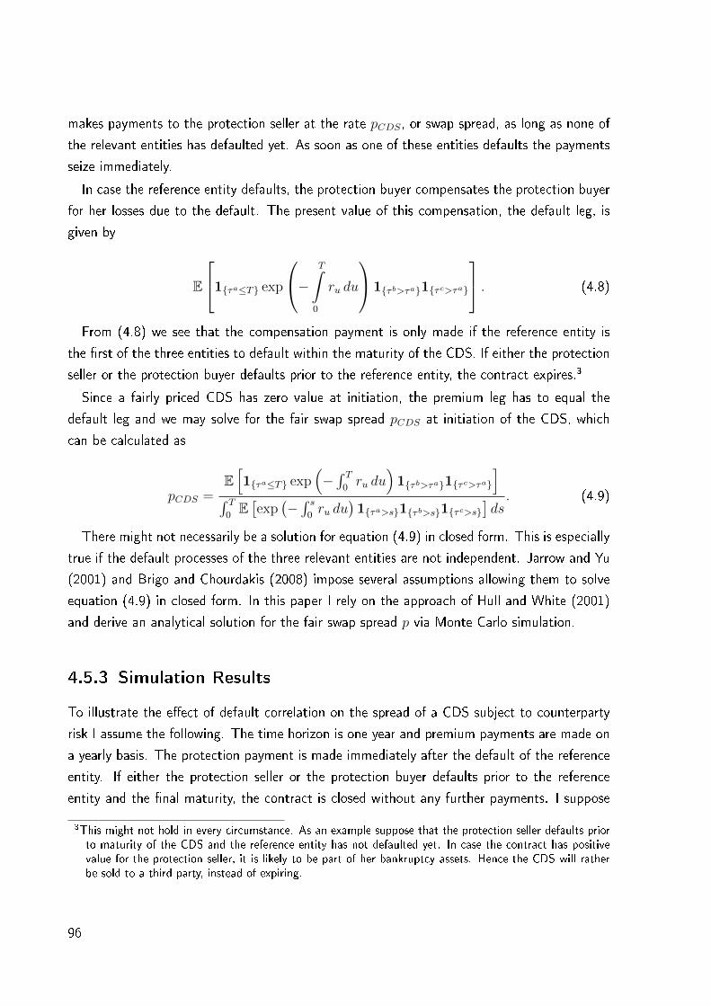
makes payments to the protection seller at the rate pCDS, or swap spread, as long as none of
the relevant entities has defaulted yet. As soon as one of these entities defaults the payments
seize immediately.
In case the reference entity defaults, the protection buyer compensates the protection buyer
for her losses due to the default. The present value of this compensation, the default leg, is
given by
E
1τa≤T exp
− T∫0
ru du
1τb>τa1τc>τa
. (4.8)
From (4.8) we see that the compensation payment is only made if the reference entity is
the rst of the three entities to default within the maturity of the CDS. If either the protection
seller or the protection buyer defaults prior to the reference entity, the contract expires.3
Since a fairly priced CDS has zero value at initiation, the premium leg has to equal the
default leg and we may solve for the fair swap spread pCDS at initiation of the CDS, which
can be calculated as
pCDS =E[1τa≤T exp
(−∫ T0ru du
)1τb>τa1τc>τa
]∫ T0E[exp
(−∫ s0ru du
)1τa>s1τb>s1τc>s
]ds. (4.9)
There might not necessarily be a solution for equation (4.9) in closed form. This is especially
true if the default processes of the three relevant entities are not independent. Jarrow and Yu
(2001) and Brigo and Chourdakis (2008) impose several assumptions allowing them to solve
equation (4.9) in closed form. In this paper I rely on the approach of Hull and White (2001)
and derive an analytical solution for the fair swap spread p via Monte Carlo simulation.
4.5.3 Simulation Results
To illustrate the eect of default correlation on the spread of a CDS subject to counterparty
risk I assume the following. The time horizon is one year and premium payments are made on
a yearly basis. The protection payment is made immediately after the default of the reference
entity. If either the protection seller or the protection buyer defaults prior to the reference
entity and the nal maturity, the contract is closed without any further payments. I suppose
3This might not hold in every circumstance. As an example suppose that the protection seller defaults priorto maturity of the CDS and the reference entity has not defaulted yet. In case the contract has positivevalue for the protection seller, it is likely to be part of her bankruptcy assets. Hence the CDS will ratherbe sold to a third party, instead of expiring.
96
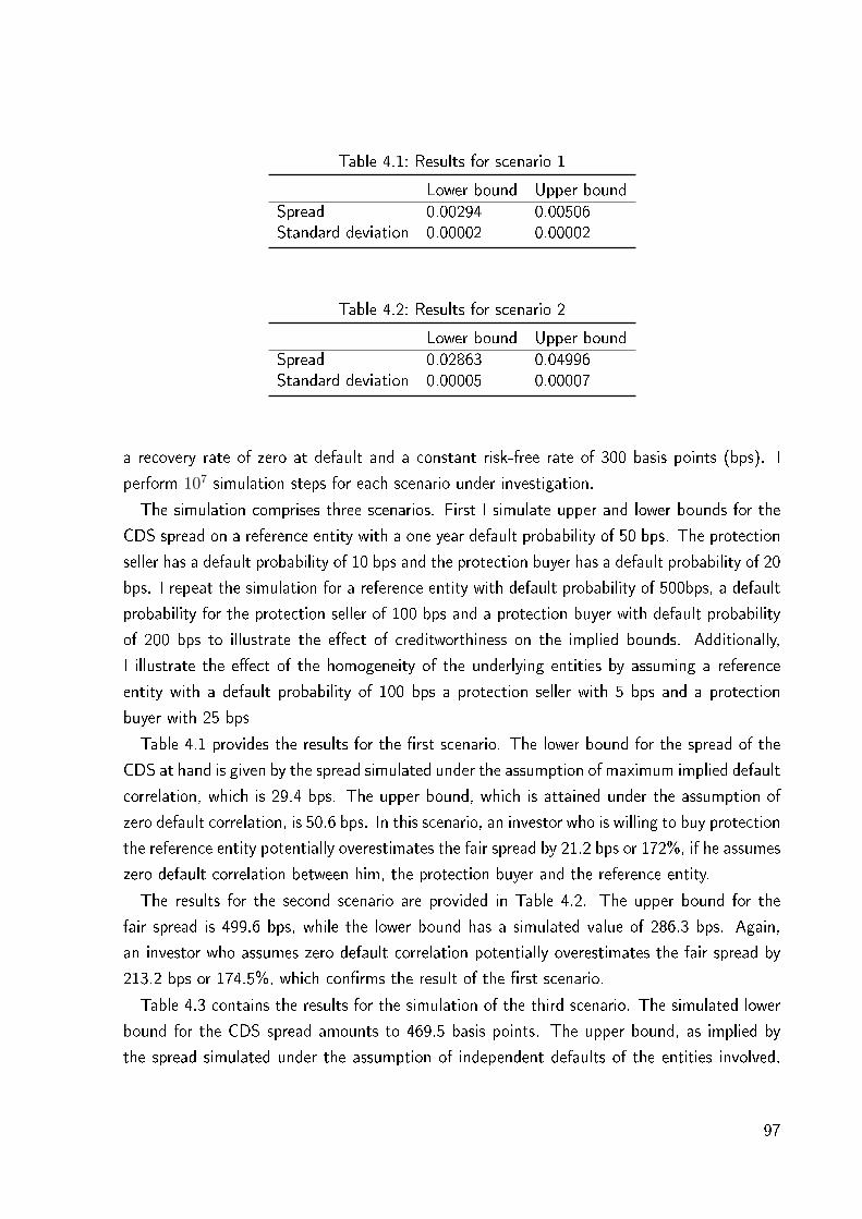
Table 4.1: Results for scenario 1
Lower bound Upper boundSpread 0.00294 0.00506Standard deviation 0.00002 0.00002
Table 4.2: Results for scenario 2
Lower bound Upper boundSpread 0.02863 0.04996Standard deviation 0.00005 0.00007
a recovery rate of zero at default and a constant risk-free rate of 300 basis points (bps). I
perform 107 simulation steps for each scenario under investigation.
The simulation comprises three scenarios. First I simulate upper and lower bounds for the
CDS spread on a reference entity with a one year default probability of 50 bps. The protection
seller has a default probability of 10 bps and the protection buyer has a default probability of 20
bps. I repeat the simulation for a reference entity with default probability of 500bps, a default
probability for the protection seller of 100 bps and a protection buyer with default probability
of 200 bps to illustrate the eect of creditworthiness on the implied bounds. Additionally,
I illustrate the eect of the homogeneity of the underlying entities by assuming a reference
entity with a default probability of 100 bps a protection seller with 5 bps and a protection
buyer with 25 bps
Table 4.1 provides the results for the rst scenario. The lower bound for the spread of the
CDS at hand is given by the spread simulated under the assumption of maximum implied default
correlation, which is 29.4 bps. The upper bound, which is attained under the assumption of
zero default correlation, is 50.6 bps. In this scenario, an investor who is willing to buy protection
the reference entity potentially overestimates the fair spread by 21.2 bps or 172%, if he assumes
zero default correlation between him, the protection buyer and the reference entity.
The results for the second scenario are provided in Table 4.2. The upper bound for the
fair spread is 499.6 bps, while the lower bound has a simulated value of 286.3 bps. Again,
an investor who assumes zero default correlation potentially overestimates the fair spread by
213.2 bps or 174.5%, which conrms the result of the rst scenario.
Table 4.3 contains the results for the simulation of the third scenario. The simulated lower
bound for the CDS spread amounts to 469.5 basis points. The upper bound, as implied by
the spread simulated under the assumption of independent defaults of the entities involved,
97
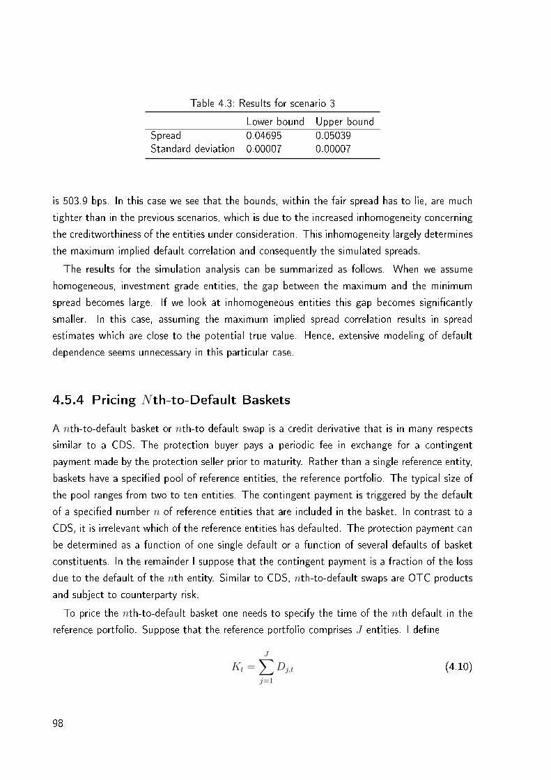
Table 4.3: Results for scenario 3
Lower bound Upper boundSpread 0.04695 0.05039Standard deviation 0.00007 0.00007
is 503.9 bps. In this case we see that the bounds, within the fair spread has to lie, are much
tighter than in the previous scenarios, which is due to the increased inhomogeneity concerning
the creditworthiness of the entities under consideration. This inhomogeneity largely determines
the maximum implied default correlation and consequently the simulated spreads.
The results for the simulation analysis can be summarized as follows. When we assume
homogeneous, investment grade entities, the gap between the maximum and the minimum
spread becomes large. If we look at inhomogeneous entities this gap becomes signicantly
smaller. In this case, assuming the maximum implied spread correlation results in spread
estimates which are close to the potential true value. Hence, extensive modeling of default
dependence seems unnecessary in this particular case.
4.5.4 Pricing Nth-to-Default Baskets
A nth-to-default basket or nth-to default swap is a credit derivative that is in many respects
similar to a CDS. The protection buyer pays a periodic fee in exchange for a contingent
payment made by the protection seller prior to maturity. Rather than a single reference entity,
baskets have a specied pool of reference entities, the reference portfolio. The typical size of
the pool ranges from two to ten entities. The contingent payment is triggered by the default
of a specied number n of reference entities that are included in the basket. In contrast to a
CDS, it is irrelevant which of the reference entities has defaulted. The protection payment can
be determined as a function of one single default or a function of several defaults of basket
constituents. In the remainder I suppose that the contingent payment is a fraction of the loss
due to the default of the nth entity. Similar to CDS, nth-to-default swaps are OTC products
and subject to counterparty risk.
To price the nth-to-default basket one needs to specify the time of the nth default in the
reference portfolio. Suppose that the reference portfolio comprises J entities. I dene
Kt =J∑j=1
Dj,t (4.10)
98

as the number of reference entities that have defaulted up to time t. The point in time of the
nth default is denoted by
τn = inf t : Kt ≥ n . (4.11)
I suppose that there is zero recovery at default. Furthermore, to come up with general results,
I assume that both the protection buyer and the protection seller may default. Every member
of the reference pool has a notional principle of 1. The protection seller continues to make
periodic payments at the rate pBasket unless Kt ≤ n or until maturity T , given that the
protection seller has not yet defaulted. Hence the premium leg can be expressed as
E
T∫0
exp
− s∫0
ru du
pBasket1τn>s1τb>s1τc>s ds
=
pBasket
T∫0
E
exp
− s∫0
ru du
1τn>s1τb>s1τc>s
ds,(4.12)
where E denotes the risk neutral expectation with respect to Ft.
In case the reference entity defaults, the protection buyer compensates the protection seller
for her losses due to the default of entity n, given that both the protection seller and the
protection buyer have survived up to time τn. The present value of this compensation, the
default leg, is given by
E
1τn≤T exp
− T∫0
ru du
1τb>τn1τc>τn
. (4.13)
For the nth-to-default basket to be fairly priced, the present value of the premium leg has
to equal the present value of the default leg. Solving for the fair premium pBasket I obtain
pBasket =E[1τn≤T exp
(−∫ T0ru du
)1τb>τn1τc>τn
]∫ T0E[exp
(−∫ s0ru du
)1τn>s1τb>s1τc>s
]ds. (4.14)
Equation (4.14) represents the most general case as the protection seller as well as the
protection buyer is subject to default risk. Although there might not be a closed form solution
to it, it can easily be solved numerically via Monte Carlo simulation. This is done in the next
section.
99

4.5.5 Simulation Results
In order to illustrate the eects of the maximum implied default correlation concept on the
pricing of nth-to-default basket, I perform several tasks. For computational ease, I examine
a basket with three reference entities and perform simulations for the 1st-, 2nd- and 3rd-to-
default swap of this illustrative basket. For simplicity, I assume that there is no counterparty
risk involved. Throughout the simulations I rely on the assumption that the default probabili-
ties of the reference entities as well as the risk-free rate are constant through time. I choose
a time horizon of one year and yearly premium payments. The default premium is paid imme-
diately after the n-th reference entity defaults. The recovery is set to be zero. I choose a risk
free rate of 300 bps and perform 107 simulation steps for each scenario under investigation.
Although these are restrictive assumptions they allow me to illustrate the eects of default
correlation while keeping computation time in reasonable levels. The simulations focus on
two main aspects. First, I derive the upper and lower bounds for the defaults swaps on the
basket to illustrate the eect of default correlation. Second, I illustrate the eect homogeneity
of entities within the basket has on the pricing of the tranches. For this purpose I vary the
relative spread dierences of the entities included in the basket.
Derivation of Bounds
I simulate fair spreads for the independence case and the maximum implied default correla-
tion case. I start with a basket of investment grade issuers (P(A)=0.00065, P(B) = 0.004,
P(B)=0.007) and repeat the simulation for a basket consisting of non-investment grade issuers
(P (A)=380 bps, P (B)=800 bps, P (C)=1290 bps). In order to provide a better understanding
of the eect of default correlation I also include spread estimates for a given default correlation
of 10% between all basket constituents. This gives a hint of how conservative the bounds are.
100
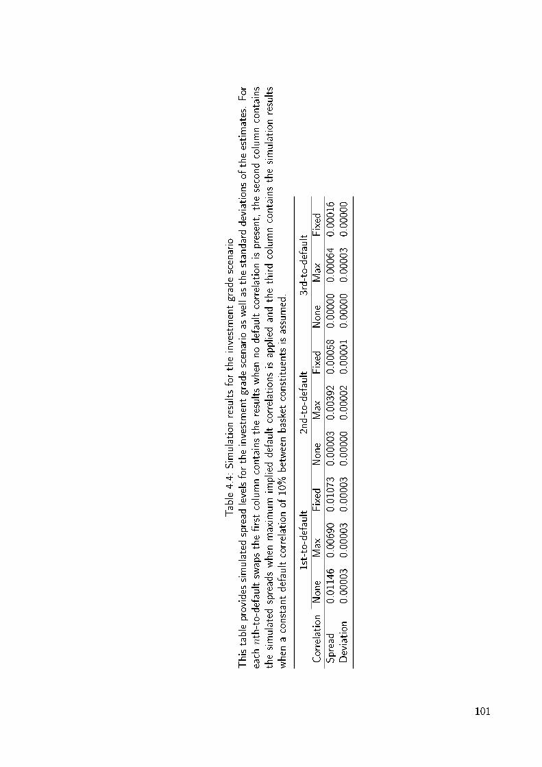
Table4.4:
Simulation
resultsfortheinvestmentgradescenario
Thistableprovides
simulatedspread
levelsfortheinvestmentgradescenarioas
wellas
thestandarddeviationsof
theestimates.For
each
nth-to-defaultswapstherstcolumncontainstheresultswhen
nodefaultcorrelationispresent,thesecondcolumncontains
thesimulatedspreadswhen
maximum
implieddefaultcorrelationsisappliedandthethirdcolumncontainsthesimulation
results
when
aconstantdefaultcorrelationof
10%
betweenbasketconstituents
isassumed.
1st-to-default
2nd-to-default
3rd-to-default
Correlation
None
Max
Fixed
None
Max
Fixed
None
Max
Fixed
Spread
0.01146
0.00690
0.01073
0.00003
0.00392
0.00058
0.00000
0.00064
0.00016
Deviation
0.00003
0.00003
0.00003
0.00000
0.00002
0.00001
0.00000
0.00003
0.00000
101

Table 4.4 contains the bounds for 3rd-, 2nd- and 1st-to default swaps on the basket of
investment grade reference entities. The results for the 3rd-to-default basket, which is most
sensitive to default dependence, show that the upper bound of the spread level is much
higher (6.4 bps) than the spread in the independence case, which is close to zero due to
diversication eects. Obviously the maximum implied default correlation method allows for
only very moderate diversication eects. In fact the fair spread is close to the spread we
would expect on a CDS on the best issuer in the basket. In the independence case the spread
is indistinguishable from zero, i.e. the probability of all three counterparties defaulting within
a one year horizon is close to zero. Hence, the possible impact of default correlation on
our 3rd-to-default swap written on the basket at hand is as large as approximately 6.4 bps,
which is not much in absolute terms but enormous on a relative basis. As expected, the
spread for an assumed default correlation of 10% lies within the bounds manifested by the
zero dependence and the maximum implied correlation case. The simulated spread for a 3rd-
to-default basket amounts to 1.6 bps or 26% of the maximum implied spread. Accordingly an
investor assuming a default correlation of 10% potentially underestimates the true spread by
a factor of approximately four.
The results for the 2nd-to-default swap are similar. Again, the upper spread bound (39bps)
is far from the independence spread (0.3 bps). The simulated spread for the moderate default
correlation (5.8 bps) is also signicantly lower. The potential eect of assumptions concerning
default correlation on the 2nd-to-default swap amount to 38.7 bps. Again, the method of
maximum implied default correlation yields only very limited diversication eects and can be
regarded as a very conservative estimate.
In line with expectations, the results for the 1st-to-default swap are dierent from the pre-
vious ones. In case the eect of maximum implied default correlation works in the opposite
direction, i.e. the probability of observing one or more defaults is lower than in the indepen-
dence case. The maximum implied default correlation spread, which is a lower bound of the
1st-to-default swap spread, amounts to 69.0 bps, while the independence spread is at 114.6
bps, which is 66% higher on a relative basis. The spread for the moderate default correlation
of 10% is in between the bounds and amounts to 107 bps. This conrms that the holders
of tranches absorbing the rst losses actually benet from higher default correlations, while
holding individual default probabilities xed.
102
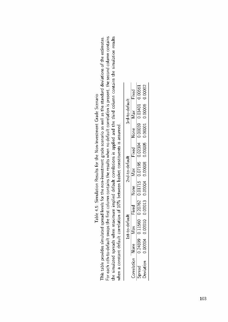
Table4.5:
Simulation
ResultsfortheNon-InvestmentGradeScenario
Thistableprovides
simulatedspread
levelsforthenon-investmentgradescenarioas
wellas
thestandarddeviationsof
theestimates.
For
eachnth-to-defaultswapstherstcolumncontainstheresultswhen
nodefaultcorrelationispresent,thesecondcolumncontains
thesimulatedspreadswhen
maximum
implieddefaultcorrelationsisappliedandthethirdcolumncontainsthesimulation
results
when
aconstantdefaultcorrelationof
10%
betweenbasketconstituents
isassumed.
1st-to-default
2nd-to-default
3rd-to-default
Correlation
None
Max
Fixed
None
Max
Fixed
None
Max
Fixed
Spread
0.24899
0.11560
0.20762
0.01715
0.07195
0.02304
0.00039
0.03401
0.00561
Deviation
0.00004
0.00010
0.00013
0.00004
0.00008
0.00005
0.00001
0.00006
0.00002
103

The results for the non-investment grade issuers are given in table 4.5. In general they
resemble the results of the previous analysis. The simulated upper bound for the 3rd-to-
default basket is 340.1 bps. In case we assume independence of defaults, the simulated spread
amounts to 3.9 bps, which is signicantly lower. In our case the possible range of inuence
concerning assumptions on the default dependence is as large as 337 bps. Put dierently, an
investor assuming zero default correlation between the three entities contained in the basket
potentially underestimates the spread by a factor of almost 100. This result emphasizes
the large inuence default dependence on portfolio products. The simulated spread for an
assumed default correlation lies in between the two bounds, as expected and amounts to 56.1
bps. Assuming a default correlation of 10% increases the spread by a factor of 14.4 compared
to the assumption of independent defaults.
For the 2nd-to-default basket the simulated upper bound of the spread is 719.4 bps, while
under the assumption of independence it amounts to 171.5 bps. This shows that in rela-
tive terms the gap between the two spreads is reduced for the non-investment grade issuers
compared to the investment grade case.
For the 1st-to default swap, the spread obtained under the assumption of maximum implied
default correlation represents the lower bound for the spread level. It amounts to 1156 bps.
The simulated spread for an assumed default correlation of 10% is 207.6 bps almost twice the
lower spread bound.
In general the results point to the fact that the method of maximum implied default cor-
relation provides very conservative spread estimates. As a consequence the upper and lower
bounds of the spreads simulated for the independence and the maximum implied correlation
case are far apart on a relative basis especially for nth-to default spreads with large n. How-
ever, this comes as no surprise since under the assumption of independence a clustering of
defaults is unlikely. Under moderate dependence assumptions, the simulated spreads are closer
to the implied upper bounds, but still signicantly lower. One might argue that for this reason
the method of maximum implied default correlation is of limited use. However, the recent
nancial crisis has shown that default correlations appear to be much higher than previously
estimated. This is especially true if a common factor driving defaults, possibly unobservable, is
not included in the pricing model. Since the method of maximum implied correlation provides
conservative estimates, the danger of underestimating the dependence is signicantly reduced.
Therefore, it can be regarded as a tool for stress testing nancial instruments that are sensitive
to the assumptions concerning default correlation.
Eects of the homogeneity of the reference pool
104

To examine the eects of homogeneity within the reference assets of the 3rd-to-default basket,
I repeat the simulation by xing the default probability of the best reference entity in the basket
and allowing the default probability of the second best and worst entity to increase with every
simulation step. The dierence between the default probability of the second and third entity
is either kept constant or is increased as well. The initial parameters are the same as in the
investment grade scenario.
Figure 4.2 illustrates the eect of varying the homogeneity of the reference entities underlying
the 3rd-to-default basket by xing the default probability of the best entity and xing the
dierence between the second best and the worst entity. The black dots represent the simulated
spread levels and the blue line is the tted spread as a function of the PD-gap between the
best and the second best reference entity. We see that, although the maximum implied spread
correlation between the rst and the second best entity in the basket constantly declines, the
maximum implied spread of the 3rd-to-default basket decreases only slowly. Overall it lies only
slightly below 5 bps, i.e. the diversication eects within the basket are only moderate. In case
we have no correlation between the assets, the spread would decline much more rapidly. We
would expect a similar eect when the default correlation within the basket declines. However,
we do not observe a signicant decline.
The explanation of this result is the following. Although the default correlation between
the best and the second best entity of the basket constantly declines, the diversication eect
is limited. To understand why, think of a simple example. On the one hand we have an
investment grade issuer, which is supposed to default in only very few cases. On the other
hand we have an entity of limited credit quality that will default in a lot of cases. If there is
measurable default correlation between the two, this means that in case the investment grade
issuer defaults, the weaker entity is quite sure to default simultaneously. Otherwise, we would
not be able to measure a signicant default correlation between the two. In our case the
best entity has a default probability of 5 bps, which is approximately the default probability
of an A-rated entity according to historical default rates. The other two entities have default
probabilities up to 400 bps. Hence, in order to have a measurable default correlation between
the entities, a default of the best entity is accompanied almost surely by the default of the
other two entities. This is why diversication eects are not pronounced when calculating
spreads based on the method of maximum implied default correlation. This observation seems
to be restrictive and limits the use of the maximum implied default correlation method. On the
other hand there might be good reasons to accept this restriction. To put it in an economic
context, the method suggests that the default of an entity with very good credit quality will
105
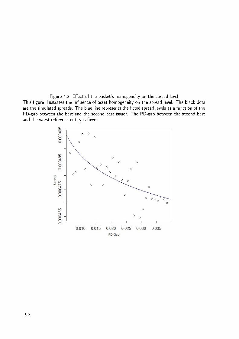
Figure 4.2: Eect of the basket's homogeneity on the spread levelThis gure illustrates the inuence of asset homogeneity on the spread level. The black dotsare the simulated spreads. The blue line represents the tted spread levels as a function of thePD-gap between the best and the second best issuer. The PD-gap between the second bestand the worst reference entity is xed.
106

be accompanied by the default of speculative grade entities. If we suppose that investment
grade AAA obligors only default in case of a systemic crisis, it is not unrealistic to assume that
this crisis will force many speculative grade issuers into default as well.
In a next step I further examine the eect of homogeneity between the reference assets by
xing the default probability of the best asset and letting the default probabilities of the other
two increase. For each simulation step the default probability of the worst entity increases
twice as much as the one of the second best entity. Therefore, the degree of homogeneity
within the pool is lowered for every simulation step.
Figure 4.3 illustrates the eect of homogeneity on the maximum implied spread of the 3rd-
to-default swap on the asset pool. The dots represent the simulated spreads and the blue
line represents the spread level as a function of the PD-gap between the best and the second
best reference entity, when the PD-gap between the second best and worst reference entity is
increased. The red line represents the tted spread level when the PD-gap between the second
best and the worst reference entity is xed, as in the previous example. Again, the method of
maximum implied default correlation hampers diversication eects. However, the additional
heterogeneity introduced by allowing the gap between the default probability of the second
and third best entity to vary, decreases spread levels. Hence, the more heterogeneous the
asset pool is composed, the lower is the maximum implied spread of the nth-to default basket,
for n greater than one. This is because the more heterogeneous the assets are, the lower
are their potential maximum implied default correlations and consequently the probability of
simultaneous defaults.
From the above examples, we see that the method of maximum implied default correlation
accounts for diversication eects. However, the eect is much less pronounced than for other
approaches, e.g. an independence assumption or the Gaussian copula. Therefore the method
yield very conservative estimates concerning the spreads of portfolio products. Nevertheless,
this might be desirable, e.g. to stress test the dependence structures of certain products to
come up with estimates of how large the impact of misspecied default correlations might be.
4.6 An Alternative Use: Comparing Dierent
Dependence Assumptions
Due to the very conservative nature of my approach, the practical relevance besides stress
testing applications seems limited. However, the approach can be used to compare dierent
assumptions concerning the dependence structure of defaults. This is achieved by compar-
ing the spreads generated by the maximum implied default correlation method with spreads
107
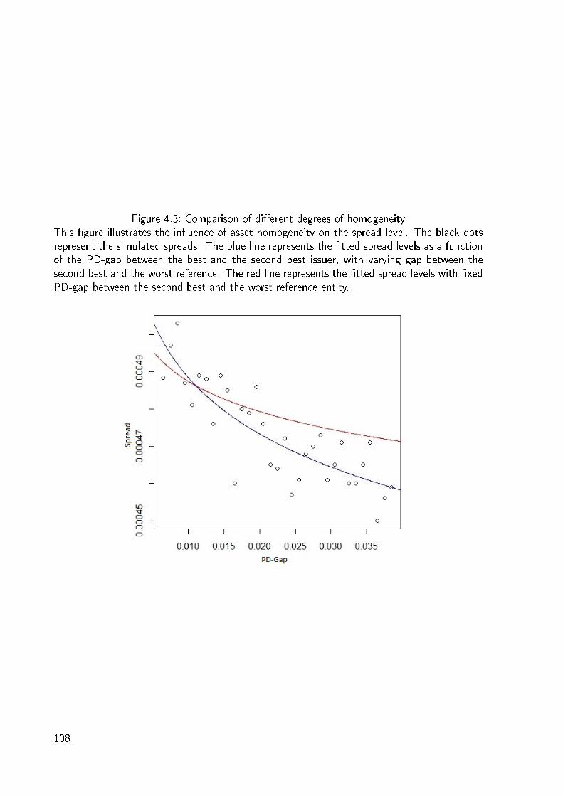
Figure 4.3: Comparison of dierent degrees of homogeneityThis gure illustrates the inuence of asset homogeneity on the spread level. The black dotsrepresent the simulated spreads. The blue line represents the tted spread levels as a functionof the PD-gap between the best and the second best issuer, with varying gap between thesecond best and the worst reference. The red line represents the tted spread levels with xedPD-gap between the second best and the worst reference entity.
108
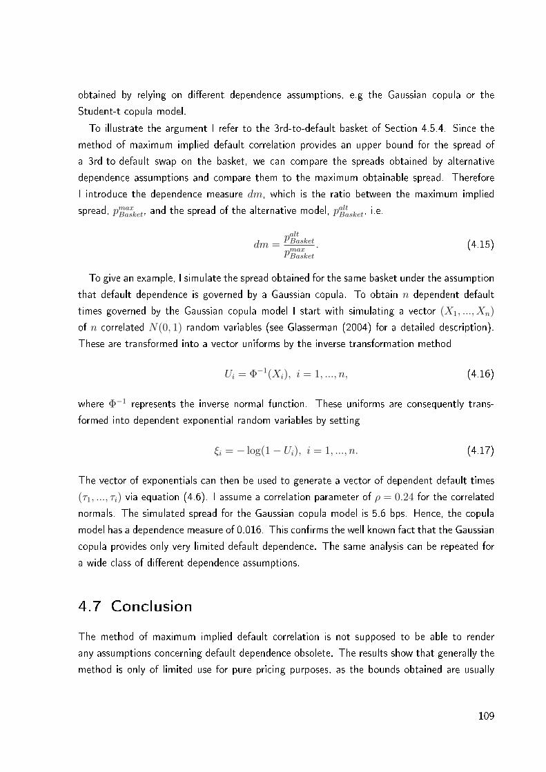
obtained by relying on dierent dependence assumptions, e.g the Gaussian copula or the
Student-t copula model.
To illustrate the argument I refer to the 3rd-to-default basket of Section 4.5.4. Since the
method of maximum implied default correlation provides an upper bound for the spread of
a 3rd-to-default swap on the basket, we can compare the spreads obtained by alternative
dependence assumptions and compare them to the maximum obtainable spread. Therefore
I introduce the dependence measure dm, which is the ratio between the maximum implied
spread, pmaxBasket, and the spread of the alternative model, paltBasket, i.e.
dm =paltBasketpmaxBasket
. (4.15)
To give an example, I simulate the spread obtained for the same basket under the assumption
that default dependence is governed by a Gaussian copula. To obtain n dependent default
times governed by the Gaussian copula model I start with simulating a vector (X1, ..., Xn)
of n correlated N(0, 1) random variables (see Glasserman (2004) for a detailed description).
These are transformed into a vector uniforms by the inverse transformation method
Ui = Φ−1(Xi), i = 1, ..., n, (4.16)
where Φ−1 represents the inverse normal function. These uniforms are consequently trans-
formed into dependent exponential random variables by setting
ξi = − log(1− Ui), i = 1, ..., n. (4.17)
The vector of exponentials can then be used to generate a vector of dependent default times
(τ1, ..., τi) via equation (4.6). I assume a correlation parameter of ρ = 0.24 for the correlated
normals. The simulated spread for the Gaussian copula model is 5.6 bps. Hence, the copula
model has a dependence measure of 0.016. This conrms the well known fact that the Gaussian
copula provides only very limited default dependence. The same analysis can be repeated for
a wide class of dierent dependence assumptions.
4.7 Conclusion
The method of maximum implied default correlation is not supposed to be able to render
any assumptions concerning default dependence obsolete. The results show that generally the
method is only of limited use for pure pricing purposes, as the bounds obtained are usually
109
far apart. Nevertheless, the method seems to be well suited to asses the impact default
correlation can potentially have on a given security. By deriving the upper and lower bounds
for spreads on such products, market participant are able to get an understanding of the actual
risk behind a certain security, without having to rely on a cumbersome modeling approach,
which in turn is likely to be very sensitive concerning its underlying assumptions. The method
of maximum implied default correlation can therefore be understood as a possible way to stress
portfolio products with regards to default correlations within their underlying reference pool.
Furthermore, the method provides a benchmark to assess the degree of default dependence
that is produced by specic assumptions, such as the Gaussian copula, by relating the result
obtained with a certain assumptions to the result of the method of maximum implied default
correlation.
110

Bibliography
Brigo, Damiano and Kyriakos Chourdakis (2008): Counterparty risk for credit default swaps:
Impact of spread volatility and default correlation, Working Paper, Fitch Solutions.
Chen, Zhiyong and Paul Glasserman (2008): Fast pricing of basket default swaps, Operations
Research 56: 286303.
Due, Darrell and Nicolae Gârleanu (2001): Risk and valuation of collateralized debt obliga-
tions, Financial Analysts Journal 57: 4159.
Due, Darrell and Kenneth Singelton (1999): Simulating correlated defaults, Working Paper,
Stanford University.
Frey, Rüdiger and Alexander McNeil (2003): Dependent defaults in models of porfolio credit
risk, Journal of Risk 6: 5992.
Giesecke, Kay and Baeho Kim (2011): Risk analysis of collateralized debt obligations, Opera-
tions Reasearch 59: 3249.
Giesecke, Kay, Baeho Kim, and Shilin Zhu (2011): Monte carlo algorithms for default timing
problems, Working Paper, Standford University and Korea University Business School.
Glasserman, Paul (2004): Monte Carlo Methods in Financial Engeneering (Springer, New
York).
Harrison, J. Michael and David M. Kreps (1979): Martingales and arbitrage in multiperiod
securities markets, Journal of Economic Theory 20: 381408.
Harrison, J. Michael and Stanley R. Pliska (1981): Martingales and stochastic integrals in the
theory of continuous trading, Stochastic Processes and their Applications 11: 215 260.
Holgate, P. (1964): Estimation for the bivariate poisson distribution, Biometrika 51: 241245.
Hull, John and Alan White (2004): Valuation of a CDO and an nth to default CDS without
Monte Carlo simulation, Journal of Derivatives 12: 823.
Hull, John C. and Alan D. White (2001): Valuing credit default swaps II: Modeling default
correlations, Journal of Derivatives 8: 1222.
Jabbour, George, Marat Kramin, and Stephenl Young (2009): nth-to-default swaps: Valuation
and analysis, Managerial Finance 35: 2547.
111
Jarrow, Robert and Stuart Turnbull (1995): Pricing derivatives on nancial securities subject
to credit risk, Journal of Finance 50: 5385.
Jarrow, Robert A. and Fan Yu (2001): Counterparty risk and the pricing of defaultable secu-
rities, Journal of Finance 56: 17651799.
Jorion, Philippe and Gaiyan Zhang (2008): Credit contagion from counterparty risk, Working
Paper, University of California.
Joshi, Mark and Dherminder Kainth (2004): Rapid and accurate developement of prices and
greeks for nth to default credit swaps in the Li model, Quantitative Finance 4: 266275.
Lando, David (1998): On cox processes and credit risky securities, Review of Derivatives
Research 2: 99120.
Laurent, Jean-Paul and Jon Gregory (2005): Basket default swaps, CDO's and factor copulas,
Journal of Risk 7: 103122.
Leung, Seng Y. and Yue K. Kwok (2005): Credit default swap valuation with counterparty
risk, Kyoto Economic Review 74: 2545.
Li, David (2000): On default correlation: A copula function approach, Journal of Fixed Income
9: 4354.
Longsta, Francis and Arvind Rajan (2008): An empirical analysis of the pricing of collateral-
ized debt obligations, Journal of Finance 63: 529563.
Lucas, Douglas J. (1995): Default correlation and credit analysis, Journal of Fixed Income 4:
7687.
Madsen, Lisa and Dan Dalthorp (2007): Simulating correlated count data, Environmental and
Ecological Statistics 14: 129148.
Mashal, Roy and Marco Naldi (2005): Pricing multi-name default swaps with counterparty
risk, Journal of Fixed Income 14: 516.
Merton, Robert (1974): On the pricing of corporate debt: The risk structure of interest rates,
Journal of Finance 29: 449470.
Park, Chul. Gyu and Dong Wan Shin (1998): An algorithm for generating correlated random
variables in a class of innitely divisible distributions, Journal of Statistical Computation
and Simulation 61: 127139.
112

Turnbull, Stuart (2005): The pricing implications of counterparty risk for non-linear credit
products, Journal of Credit Risk 1: 333.
113
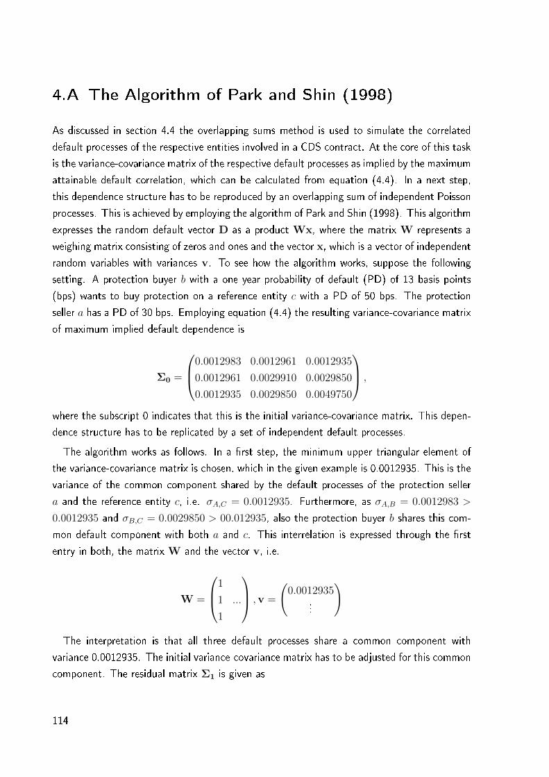
4.A The Algorithm of Park and Shin (1998)
As discussed in section 4.4 the overlapping sums method is used to simulate the correlated
default processes of the respective entities involved in a CDS contract. At the core of this task
is the variance-covariance matrix of the respective default processes as implied by the maximum
attainable default correlation, which can be calculated from equation (4.4). In a next step,
this dependence structure has to be reproduced by an overlapping sum of independent Poisson
processes. This is achieved by employing the algorithm of Park and Shin (1998). This algorithm
expresses the random default vector D as a product Wx, where the matrix W represents a
weighing matrix consisting of zeros and ones and the vector x, which is a vector of independent
random variables with variances v. To see how the algorithm works, suppose the following
setting. A protection buyer b with a one year probability of default (PD) of 13 basis points
(bps) wants to buy protection on a reference entity c with a PD of 50 bps. The protection
seller a has a PD of 30 bps. Employing equation (4.4) the resulting variance-covariance matrix
of maximum implied default dependence is
Σ0 =
0.0012983 0.0012961 0.0012935
0.0012961 0.0029910 0.0029850
0.0012935 0.0029850 0.0049750
,
where the subscript 0 indicates that this is the initial variance-covariance matrix. This depen-
dence structure has to be replicated by a set of independent default processes.
The algorithm works as follows. In a rst step, the minimum upper triangular element of
the variance-covariance matrix is chosen, which in the given example is 0.0012935. This is the
variance of the common component shared by the default processes of the protection seller
a and the reference entity c, i.e. σA,C = 0.0012935. Furthermore, as σA,B = 0.0012983 >
0.0012935 and σB,C = 0.0029850 > 00.012935, also the protection buyer b shares this com-
mon default component with both a and c. This interrelation is expressed through the rst
entry in both, the matrix W and the vector v, i.e.
W =
1
1 ...
1
,v =
(0.0012935
...
)
The interpretation is that all three default processes share a common component with
variance 0.0012935. The initial variance-covariance matrix has to be adjusted for this common
component. The residual matrix Σ1 is given as
114

Σ1 = Σ0 −
0.0012935 0.0012935 0.0012935
0.0012935 0.0012935 0.0012935
0.0012935 0.0012935 0.0012935
=
0.0000048 0.0000026 0
0.0000026 0.0016975 0.0016915
0 0.0016915 0.0036815
.
After the adjustment of the variance-covariance matrix, the rst iteration of the algorithm is
complete. In the next iteration step, again the minimum non-zero upper triangular element of
the matrix Σ1, is chosen. In the the above example this is 0.0000026, which is the variance of
the default component shared by a and b. As the residual covariance σA,C = 0 < 0.0000026, a
and c do not share this component. The matrix W and the vector v are adjusted accordingly,
i.e.
W =
1 1
1 1 · · ·1 0
,v =
0.0012935
0.0000026...
.
The residual matrix Σ2 is calculated as
Σ2 = Σ1 −
0.0000026 0.0000026 0
0.0000026 0.0000026 0
0 0 0
=
0.0000022 0 0
0 0.0016949 0.0016915
0 0.0016915 0.0036815
.
The algorithm continues until there are no more non-zero upper triangular elements in the
residual variance-covariance matrix. The remaining elements on the main diagonal, are the
idiosyncratic default components of the single counterparties. These are not shared by any
other entity. In the above example the algorithm has the nal outcome
W =
1 1 0 1 0 0
1 1 1 0 1 0
1 0 1 0 0 1
,v =
0.0012935
0.0000026
0.0016915
0.0000022
0.0000034
0.0019900
.
115

The interpretation of the above results is straightforward. To simulate the default processes
of the three entities a, b and c with the given maximum implied dependence structure Σ0,
one has to simulate six independent default processes with variances given by the vector v,
of which the rst three are contagious, leading to the simultaneous default of two or more
entities and the last three are completely idiosyncratic. For example, if the default process
with variance given by the rst entry of the vector v is the rst to default, this triggers a
simultaneous default of all three entities. In contrast if the default component with variance
given by the fourth entry of the vector v is the rst to default, this would result in a default
of entity a only.
In order to derive the default times of the entities under consideration according to equa-
tion (4.6), the variances of the default processes are converted into the respective default
probabilities.4 These, in turn, are converted into one year default intensities via
λI = − ln(1− P (I)).
4Since the variance of entity i's default process is calculated as σN = P (I)(1− P (I)), this involves solvinga quadratic equation. Hence, there are two possible solutions for the probability of default, which sum toone by construction. Of the two solutions the one which suits si is chosen. For reasonable choices of sithis will always be the smaller one.
116

5 Epilog
As outlined in section 1, this dissertation is dedicated to several research questions that
were addressed in the preceding three essays. At the core of all three essays is the relationship
between the recent subprime nancial crisis and the market for credit risk. The rst essay is
dedicated to the investigation, which causes are behind the subprime nancial crisis, the role
credit markets and credit derivatives played in the course of the crisis and how the crisis can be
resolved from a government perspective. Several circumstances contributed to the subprime
nancial crisis and credit derivatives clearly played a signicant role as an accelerant for the
transmission of the crisis throughout the nancial services industry.
In the rst essay we discuss several possibilities how the crisis might be resolved by means
of government intervention. Among these are direct recapitalization, state guarantees and
purchase programs for troubled assets. We formally show that only the latter provide the
possibility to establish a mechanism allowing to separate illiquid but solvent and insolvent
banks and therefore to resolve the uncertainty within nancial markets concerning the solvency
of individual banks. If the price oered for the troubled assets is chosen correctly, solvent and
insolvent banks will behave dierently and reveal the state they are actually in to outsiders. In
the end, all banks are better of revealing their true state than trying to mimic a solvent bank.
Given the tremendous impact of the subprime nancial crisis, it is straight forward to raise
the question, how a similar crisis can be prevented in the future. A stricter regulation of credit
markets can not be the sole conclusion drawn out of the crisis. In general the innovations in
the market for credit risk are benecial for the economy. However, it must be assured that
market participants are aware of the risks they are exposed to and act in a reasonable not
solely prot driven way.
The second essay is dedicated to the question what impact the recent subprime nancial
crisis had on market participants' perceptions of credit risk. For this purpose we conduct
an empirical analysis of the determinants of iTraxx spread changes, which can be regarded
as a measure of aggregate credit risk. We nd empirical evidence that the determinants
of iTraxx spread changes have evolved in the course of the subprime nancial crisis. This
nding suggests that market participants have altered their perceptions concerning credit risk
as a consequence of the crisis. In general, during the subprime nancial crisis, determinants
as implied by structural models of credit risk show a weakened explanatory power for iTraxx
spread changes. This is especially true if we examine the determinants of large spread changes.
A quantile regression reveals that factors, as implied by structural models of credit risk, are not
sucient to explain extreme spread changes, indicating that structural models of credit risk
need further improvement. A VARX-model reveals that the role of credit markets in processing
relevant information has changed during the subprime nancial crisis. While stock returns
118

tended to lead iTraxx spread changes before the crisis, there is a tendency of iTraxx spread
changes leading stock returns after the crisis. Hence, we conclude that market participants
rely on iTraxx spreads as a source of information concerning systemic risk in nancial markets.
Consequently, the third essay deals with the question, how complex credit derivatives can
be modeled in a way that allows for an understanding of their inherent risk, while reducing the
complexity of the modeling approach to a necessary minimum. For this purpose I introduce
the method of maximum implied default correlation. The method is based on bounds for the
default correlation of pairs of entities that can be inferred from market prices. The approach
allows for a derivation of bounds for the prices of credit derivatives that hold in the absence of
arbitrage, regardless of the true default correlation between the entities under consideration. I
propose an easy to implement Monte Carlo algorithm that allows to derive a numerical solution
for the bounds of credit derivatives that are sensitive towards default correlation. I apply the
model to two types of credit derivatives that are sensitive towards default correlation, CDSs
subject to counterparty risk and nth-to-default baskets.
While the method of maximum implied default correlation is of limited use when it comes
to the exact pricing of credit derivatives that are sensitive towards default correlation, it
proves to be a useful tool to asses the extend such products are actually exposed to default
correlation. I show that given for some products, the simulated bounds for the prices of some
credit derivatives are far apart from what one might expect given state of the art model of
default correlation, such as the Gaussian copula model. Therefore, the method of maximum
implied default correlation can be used as a benchmark for the conservativeness of dierent
assumptions concerning default correlation.
119

Bibliography
Acharya, Viral and Tanju Yorulmazer (2008): Cash-in-the-market pricing and optimal resolu-
tion of bank failures, Review of Financial Studies 21: 27052742.
Alexander, Carol and Andreas Kaeck (2008): Regime dependent determinants of credit default
swap spreads, Journal of Banking & Finance 32: 10081021.
Allen, Franklin and Elena Carletti (2010): An overview of the crisis: Causes, consequences,
and solutions, International Review of Finance 10: 126.
Amihud, Yakov (2002): Illiquidity and stock returns: Cross-section and time-series eects,
Journal of Financial Markets 5: 3156.
Amiyatosh, Purnanandam (2009): Originate-to-distribute model and the subprime mortgage
crisis, Working Paper, University of Michigan.
Bank of England (2008): Financial Stability Report October 2008, Bank of England Financial
Stability Reports, Bank of England.
Basel Committee on Banking Supervision (2004): International Convergence of Capital Mea-
surement and Capital Standards: A Revised Framework, Working Paper, Bank for Interna-
tional Settlements.
Batten, Jonathan A. and Warren P. Hogan (2009): Asia-Pacic perspective on the nan-
cial crisis 2007-2010, Working Paper, Hong Kong University of Science & Technology and
University of Technology, Sidney.
Bebchuk, Lucian A. (2008): A Plan for Addressing the Financial Crisis, Working Paper, John
M. Olin Center for Law, Economics, and Business.
Bebchuk, Lucian A. (2009): Buying troubled assets, Yale Journal on Regulation 26: 343358.
Benkert, Christoph (2004): Explaining credit default swap premia, Journal of Futures Markets
24: 7192.
Berndt, Antje, Rohan Douglas, Darrell Due, Mark Ferguson, and David Schranz (2005):
Measuring default risk premia from default swap rates and EDFs, Working Paper, Bank for
International Settlements.
120

Breitenfellner, Bastian and Niklas Wagner (2010): Coping with the nancial crisis: Illiquidity
and the role of government intervention, in Kolb, Robert, ed., Lessons from the Financial
Crisis: Causes, Consequences, and Our Economic Future (Wiley, Hoboken), pp. 579 586.
Brigo, Damiano and Kyriakos Chourdakis (2008): Counterparty risk for credit default swaps:
Impact of spread volatility and default correlation, Working Paper, Fitch Solutions.
Bryant, John (1980): A model of reserves, bank runs, and deposit insurance, Journal of
Banking & Finance 4: 335344.
Byström, Hans (2005): Credit default swaps and equity prices: The iTraxx CDS index market,
Working paper, Lund University.
Campbell, John and Glen Taksler (2002): Equity volatility and corporate bond yields, Working
Paper 1945, Harvard - Institute of Economic Research.
Chen, Zhiyong and Paul Glasserman (2008): Fast pricing of basket default swaps, Operations
Research 56: 286303.
Chow, Greogory (1960): Tests of equality between sets of coecients in two linear regressions,
Econometrica 28: 591605.
Collin-Dufresne, Pierre, Robert Goldstein, and J. Martin (2001): The determinants of credit
spread changes, Journal of Finance 56: 21772207.
Das, Sanjiv and Paul Hanouna (2009): Hedging credit: Equity liquidity matters, Journal of
Financial Intermediation 18: 112123.
Diamond, Douglas and Philip Dybvig (1983): Bank runs, deposit insurance, and liquidity,
Journal of Political Economy 91: 401419.
Diamond, Douglas and Raghuram Rajan (2002): Bank bailouts and aggregate liquidity, Amer-
ican Economic Review 92: 3841.
Diamond, Douglas and Raghuram Rajan (2005): Liquidity shortages and banking crises, Jour-
nal of Finance 60: 615647.
Due, Darrel and Nicolae Gârleanu (2001): Risk and valuation of collateralized debt obliga-
tions, Financial Analysts Journal 57: 4159.
Due, Darrel and Kenneth Singleton (2003): Credit Risk: Pricing Measurement and Man-
agement (Princeton University Press, Princeton).
121
Due, Darrell (2007): Innovations in Credit Risk Transfer: Implications for Financial Stability,
Working Paper, Bank for International Settlements.
Due, Darrell, Leandro Saita, and Ke Wang (2007): Multi-period corporate default prediction
with stochastic covariates, Journal of Financial Economics 83: 635665.
Due, Darrell and Kenneth Singelton (1999): Simulating correlated defaults, Working Paper,
Stanford University.
Due, Darrell and Kenneth Singleton (1999): Modeling term structures of defaultable bonds,
Review of Financial Studies 12: 687720.
Ericsson, Jan, Kris Jacobs, and Rodolfo Oviedo-Helfenberger (2004): The determinants of
credit default swap premia, Working Paper 32, Swedish Institute for Financial Research.
Franke, Günter and Jan Pieter Krahnen (2008): The future of securitization, Working Paper,
Center for Financial Studies.
Freixas, Xavier (1999): Optimal bail out policy, conditionality and constructive ambiguity,
Working Paper, Universitat Pompeu Fabra.
Frey, Rüdiger and Alexander McNeil (2003): Dependent defaults in models of porfolio credit
risk, Journal of Risk 6: 5992.
Fung, Hung-Gay, Gregory Sierra, Jot Yau, and Zhang Gaiyan (2008): Are the U.S. stock
market and credit default swap market related? Evidence from the CDX indices, Working
paper, University of MissouriSt. Louis.
Giammarino, Flavia and Pauline Barrieu (2009): A semiparametric model for the systematic
factors of portfolio credit risk premia, Journal of Empirical Finance 16: 655670.
Giesecke, Kay and Baeho Kim (2011): Risk analysis of collateralized debt obligations, Opera-
tions Reasearch 59: 3249.
Giesecke, Kay, Baeho Kim, and Shilin Zhu (2011): Monte Carlo algorithms for default timing
problems, Working Paper, Standford University and Korea University Business School.
Glasserman, Paul (2004): Monte Carlo Methods in Financial Engeneering (Springer, New
York).
Goodfriend, Marvin and Robert King (1988): Financial deregulation, monetary policy, and
central banking, Working Paper, Federal Reserve Bank of Richmond.
122

Gorton, Gary (2009): The subprime panic, European Financial Management 15: 1046.
Gorton, Gary and Lixin Huang (2004): Liquidity, eciency, and bank bailouts, American
Economic Review 94: 455483.
Gorton, Gary and Nicholas Souleles (2005): Special Purpose Vehicles and Securitization,
Working Paper, National Bureau of Economic Research.
Hannan, Edward and Barry Quinn (1979): The determination of the order of an autoregression,
Journal of the Royal Statistical Society. Series B (Methodological) 41: 190195.
Harrison, Michael and David Kreps (1979): Martingales and arbitrage in multiperiod securities
markets, Journal of Economic Theory 20: 381408.
Harrison, Michael and Stanley Pliska (1981): Martingales and stochastic integrals in the theory
of continuous trading, Stochastic Processes and their Applications 11: 215 260.
Holgate, P. (1964): Estimation for the bivariate poisson distribution, Biometrika 51: 241245.
Hoshi, Takeo and Anil K Kashyap (2008): Will the U.S. Bank Recapitalization Succeed?
Lessons from Japan, Working Paper, National Bureau of Economic Research.
Hull, John and Alan White (2001): Valuing credit default swaps II: Modeling default correla-
tions, Journal of Derivatives 8: 1222.
Hull, John and Alan White (2004): Valuation of a CDO and an nth to default CDS without
Monte Carlo simulation, Journal of Derivatives 12: 823.
International Monetary Fund (2003): Financial Asset Price Volatility: A Source of Instability?,
in Global Financial Stability Report, September 2003, pp. 6288.
Jabbour, George, Marat Kramin, and Stephenl Young (2009): Nth-to-default swaps: Valua-
tion and analysis, Managerial Finance 35: 2547.
Jarrow, Robert, David Lando, and Stuart Turnbull (1997): A Markov model for the term
structure of credit risk spreads, Review of Financial Studies 10: 481523.
Jarrow, Robert and Stuart Turnbull (1995): Pricing derivatives on nancial securities subject
to credit risk, Journal of Finance 50: 5385.
Jarrow, Robert and Fan Yu (2001): Counterparty risk and the pricing of defaultable securities,
Journal of Finance 56: 17651799.
123

Jorion, Philippe and Gaiyan Zhang (2008): Credit contagion from counterparty risk, Working
Paper, University of California.
Joshi, Mark and Dherminder Kainth (2004): Rapid and accurate developement of prices and
greeks for nth to default credit swaps in the Li model, Quantitative Finance 4: 266275.
Koenker, Roger and Gilbert Jr. Bassett (1978): Regression quantiles, Econometrica 46(1):
3350.
Koenker, Roger and Kevin F. Hallock (2001): Quantile regression, Journal of Economic Per-
spectives 15: 143156.
Lando, David (1998): On cox processes and credit risky securities, Review of Derivatives
Research 2: 99120.
Laurent, Jean-Paul and Jon Gregory (2005): Basket default swaps, CDO's and factor copulas,
Journal of Risk 7: 103122.
Leung, Seng and Yue Kwok (2005): Credit default swap valuation with counterparty risk,
Kyoto Economic Review 74: 2545.
Li, David (2000): On default correlation: A copula function approach, Journal of Fixed Income
9: 4354.
Longsta, Francis and Arvind Rajan (2008): An empirical analysis of the pricing of collateral-
ized debt obligations, Journal of Finance 63: 529563.
Lucas, Douglas (1995): Default correlation and credit analysis, Journal of Fixed Income 4:
7687.
Madsen, Lisa and Dan Dalthorp (2007): Simulating correlated count data, Environmental and
Ecological Statistics 14: 129148.
Markit (2010a): Markit credit indices: A primer, Technical report, Markit Group.
Markit (2010b): Markit iTraxx indices: Index level calculation, Technical report, Markit Group.
Markit (2011): Markit iTraxx Europe: Index rules, Technical report, Markit Group.
Mashal, Roy and Marco Naldi (2005): Pricing multi-name default swaps with counterparty
risk, Journal of Fixed Income 14: 516.
124
Merton, Robert (1974): On the pricing of corporate debt: The risk structure of interest rates,
Journal of Finance 29: 449470.
Merton, Robert (1977): An analytic derivation of the cost of deposit insurance and loan
guarantees - An application of modern option pricing theory, Journal of Banking & Finance
1: 311.
Mills, Paul and John Ki (2007): Money for Nothing and Checks for Free: Recent Develop-
ments in U.S. Subprime Mortgage Markets, Working Paper, International Monetary Fund.
Norden, Lars and Martin Weber (2009): The co-movement of credit default swap, bond and
stock markets: An empirical analysis, European Financial Management 15: 529562.
Pan, Jun and Kenneth Singleton (2005): Default and recovery implicit in the term structure
of sovereign CDS spreads, Working paper, MIT and Stanford.
Park, Chul. Gyu and Dong Wan Shin (1998): An algorithm for generating correlated random
variables in a class of innitely divisible distributions, Journal of Statistical Computation
and Simulation 61: 127139.
Peiderer, Paul and Terry Marsh (2009): The 2008-2009 nancial crisis: Risk model trans-
parency and incentives, Working Paper, Stanford University and Quantal International Inc.
Scheicher, Martin (2003): Credit derivatives - overview and implications for monetary policy
and nancial stability, in OeNB Financial Stability Report 5, pp. 96111.
Scheicher, Martin (2008): How has CDO market pricing changed during the turmoil?, Working
paper, European Central Bank.
Shiller, Robert J. (2008): The Subprime Solution: How Today's Global Financial Crisis Hap-
pened, and What to Do about It (Princeton University Press, Princeton).
Tang, Dragon and Hong Yan (2007): Liquidity and credit default swap spreads, Working
Paper, University of Hong Kong.
Turnbull, Stuart (2005): The pricing implications of counterparty risk for non-linear credit
products, Journal of Credit Risk 1: 333.
Wilson, Linus (2010a): A binominal model of Geithner's toxic asset plan, Working Paper,
University of Louisiana at Lafayette.
Wilson, Linus (2010b): The put problem with buying toxic assets, Applied Financial Economics
20: 3135.
125

Eidesstattliche Versicherung
Hiermit versichere ich an Eides statt, dass ich die vorliegende Dissertation mit dem Titel
Three Essays on Credit Risk with a Special Focus on the Subprime Financial Crisis selbständig,
ohne unzulässige Hilfe Dritter und ohne Benutzung anderer als der angegebenen Quellen und
Hilfsmittel verfasst habe und dass alle Ausführungen, die wörtlich oder sinngemäÿ übernommen
wurden, als solche gekennzeichnet sind.
Die Arbeit wurde bisher keiner anderen Prüfungsbehörde vorgelegt.
Datum: 20. September 2012
Bastian Breitenfellner