Embed Size (px)
Citation preview
This WEEK:Lab: last 1/2 of manuscript due Lab VII Life Table for Human Pop Bring calculator! Will complete Homework 8 in lab
Next WEEK: Homework 9 = Pop. Growth Problems Start early!
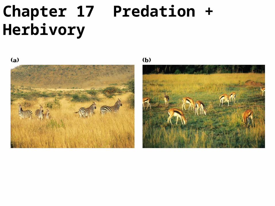
Chapter 17 Predation + Herbivory
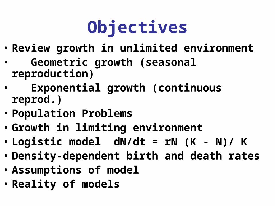
Objectives• Review growth in unlimited environment• Geometric growth (seasonal reproduction)• Exponential growth (continuous reprod.)• Population Problems• Growth in limiting environment• Logistic model dN/dt = rN (K - N)/ K• Density-dependent birth and death rates• Assumptions of model• Reality of models
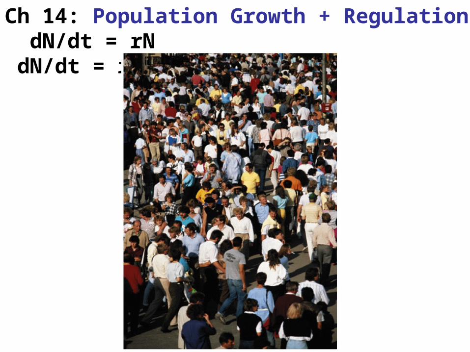
Ch 14: Population Growth + Regulation dN/dt = rN dN/dt = rN(K-N)/K
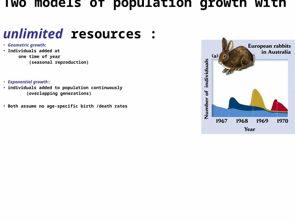
• Geometric growth:• Individuals added at one time of year (seasonal reproduction)
• Exponential growth: • individuals added to population continuously (overlapping generations)
• Both assume no age-specific birth /death rates
Two models of population growth with unlimited resources :
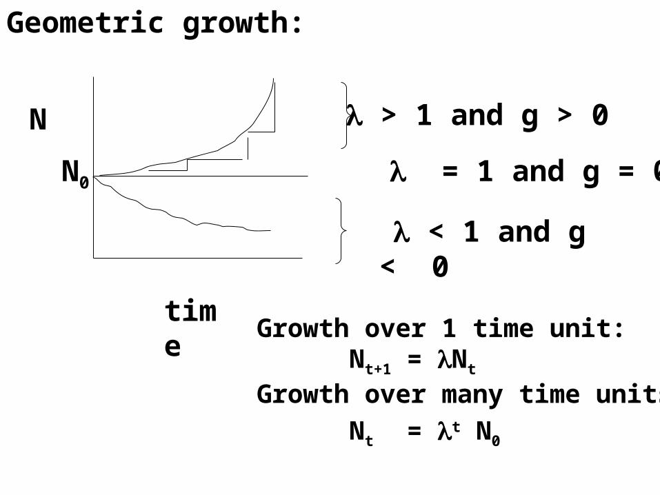
Geometric growth:
N
N0
> 1 and g > 0
= 1 and g = 0
< 1 and g < 0
time Growth over 1 time unit:
Nt+1 = Nt
Growth over many time units:
Nt = t N0
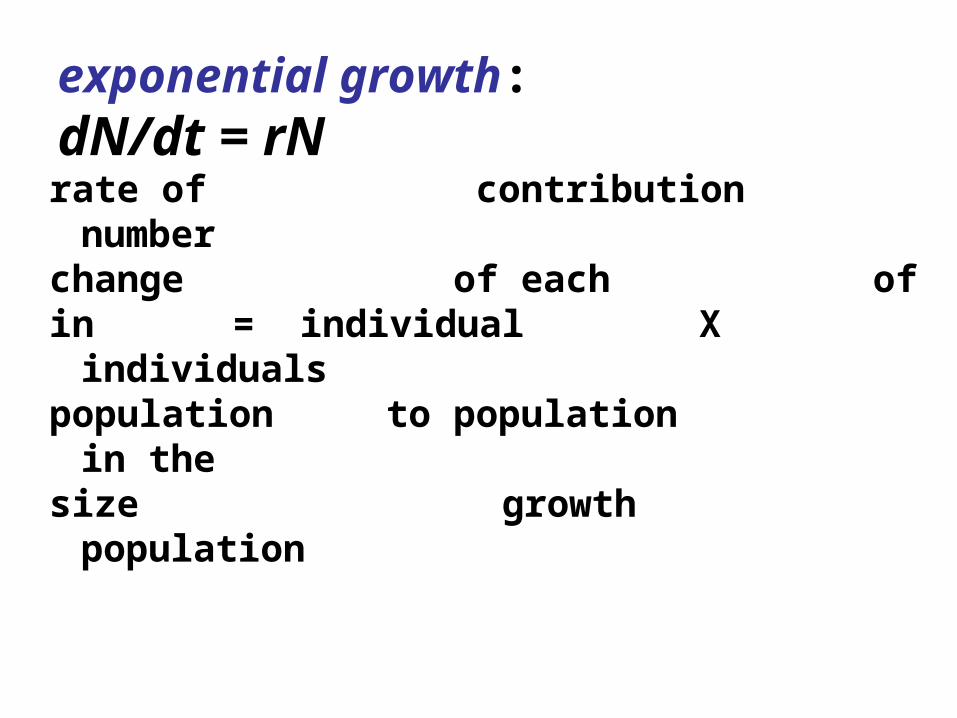
exponential growth:dN/dt = rN
rate of contribution numberchange of each of in = individual X
individualspopulation to population in thesize growth
population
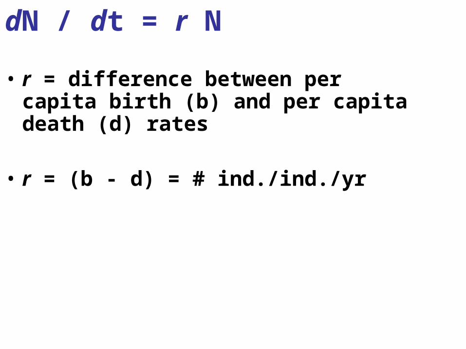
dN / dt = r N
• r = difference between per capita birth (b) and per capita death (d) rates
• r = (b - d) = # ind./ind./yr
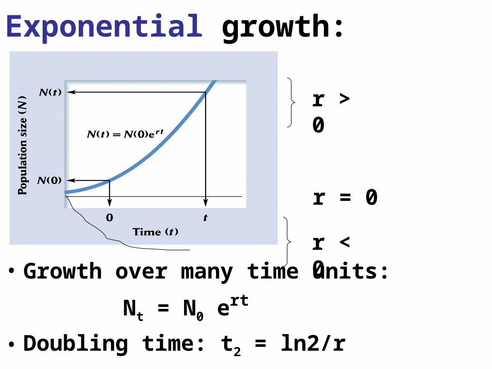
Exponential growth:
• Growth over many time units:
Nt = N0 ert
• Doubling time: t2 = ln2/r
r > 0
r < 0
r = 0
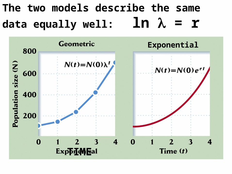
The two models describe the same data
equally well: ln = r
TIME
Exponential
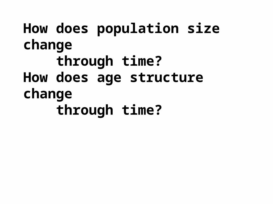
How does population size change through time?How does age structure change through time?
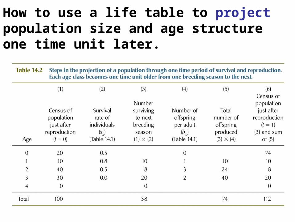
How to use a life table to project population size and age structure one time unit later.
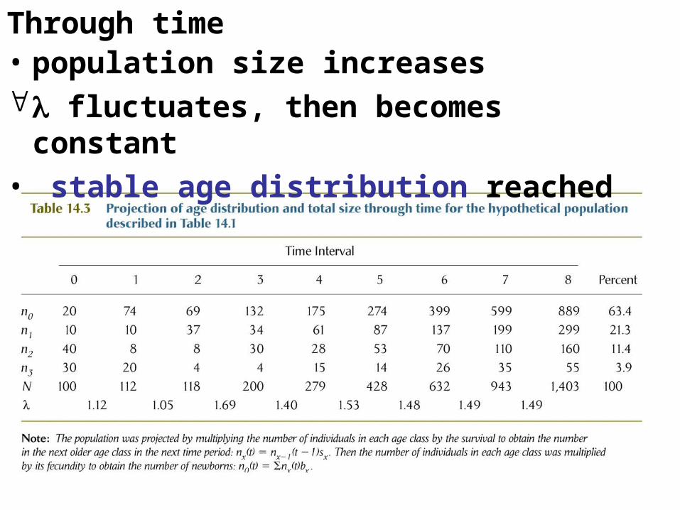
Through time• population size increases fluctuates, then becomes constant
• stable age distribution reached
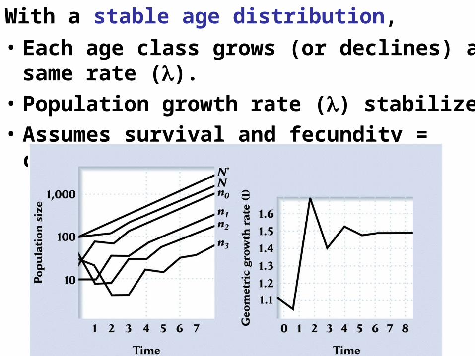
With a stable age distribution,
• Each age class grows (or declines) at same rate ().
• Population growth rate () stabilizes.
• Assumes survival and fecundity = constant.
*** What is a stable age distribution for a population and under what conditions is it reached?
• SAD = pop in which the proportions of individuals in the age classes remain constant through time
• Population can achieve a SAD only if its age-specific schedule of survival and fecundity rates remains constant through time.
• Any change in these will alter the SAD and population growth rate
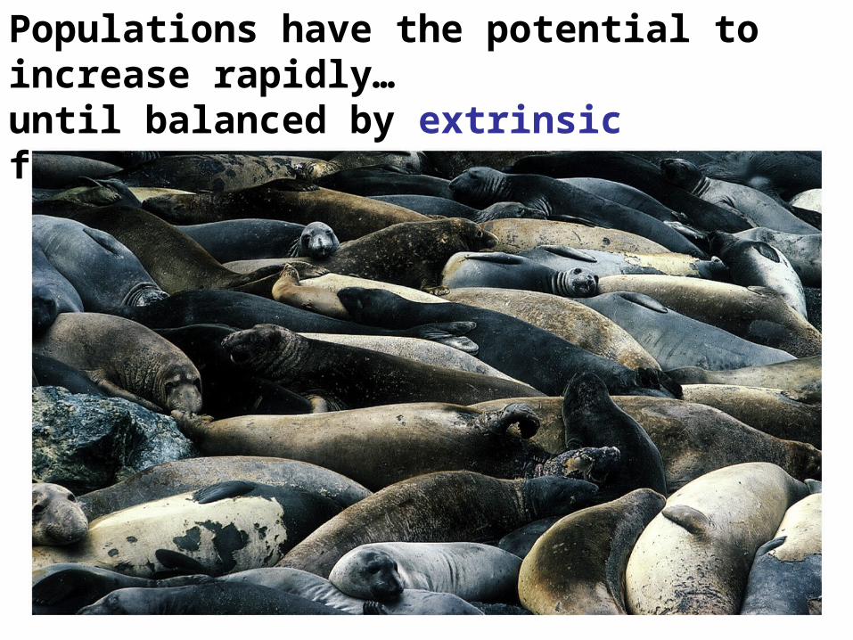
Populations have the potential to increase rapidly…until balanced by extrinsic factors.
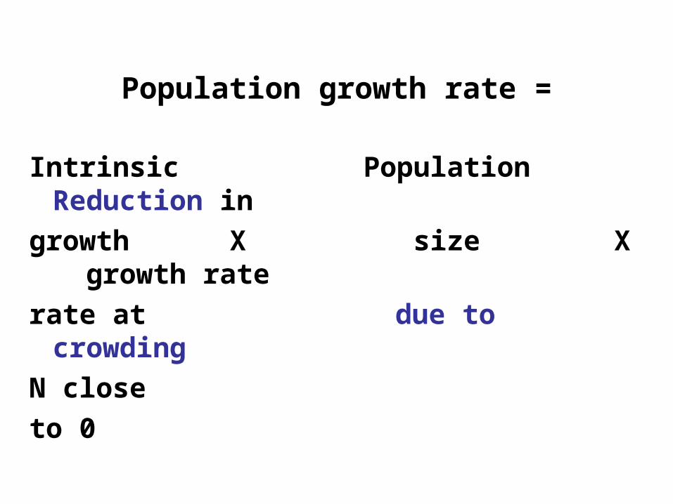
Population growth rate =
Intrinsic Population Reduction in
growth X size X growth rate
rate at due to crowding
N close
to 0
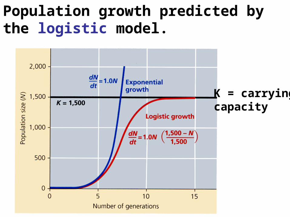
Population growth predicted by the logistic model.
K = carryingcapacity
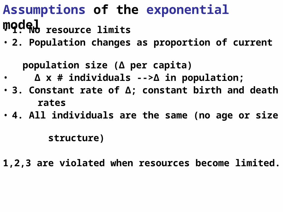
Assumptions of the exponential model
• 1. No resource limits• 2. Population changes as proportion of current
population size (∆ per capita)• ∆ x # individuals -->∆ in population;• 3. Constant rate of ∆; constant birth and death
rates• 4. All individuals are the same (no age or size structure)
1,2,3 are violated when resources become limited.
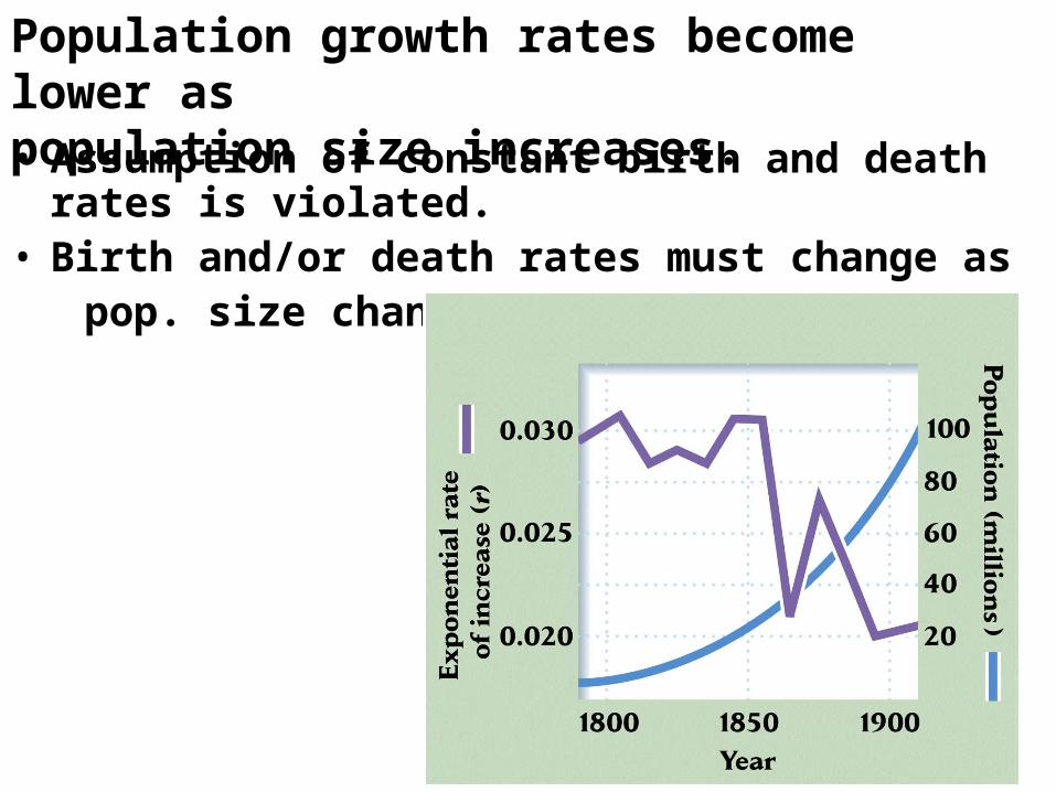
Population growth rates become lower aspopulation size increases.• Assumption of constant birth and death rates is
violated.• Birth and/or death rates must change as pop. size changes.
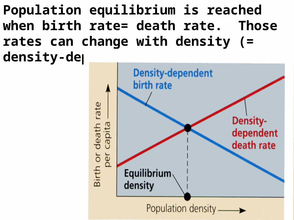
Population equilibrium is reached when birth rate= death rate. Those rates can change with density (= density-dependent).
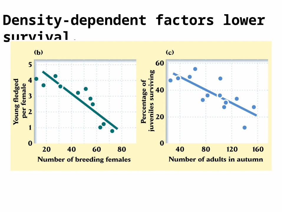
Density-dependent factors lower survival.
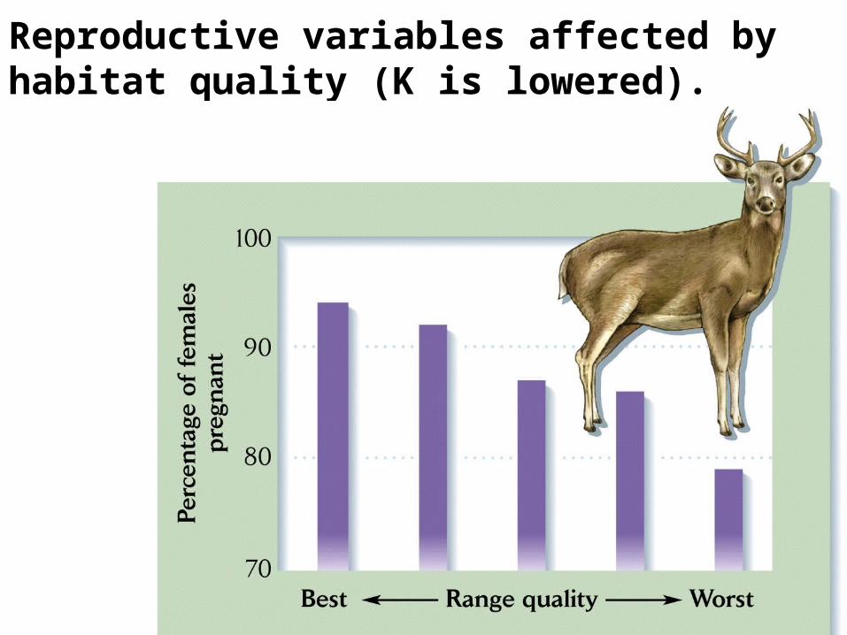
Reproductive variables affected by habitat quality (K is lowered).
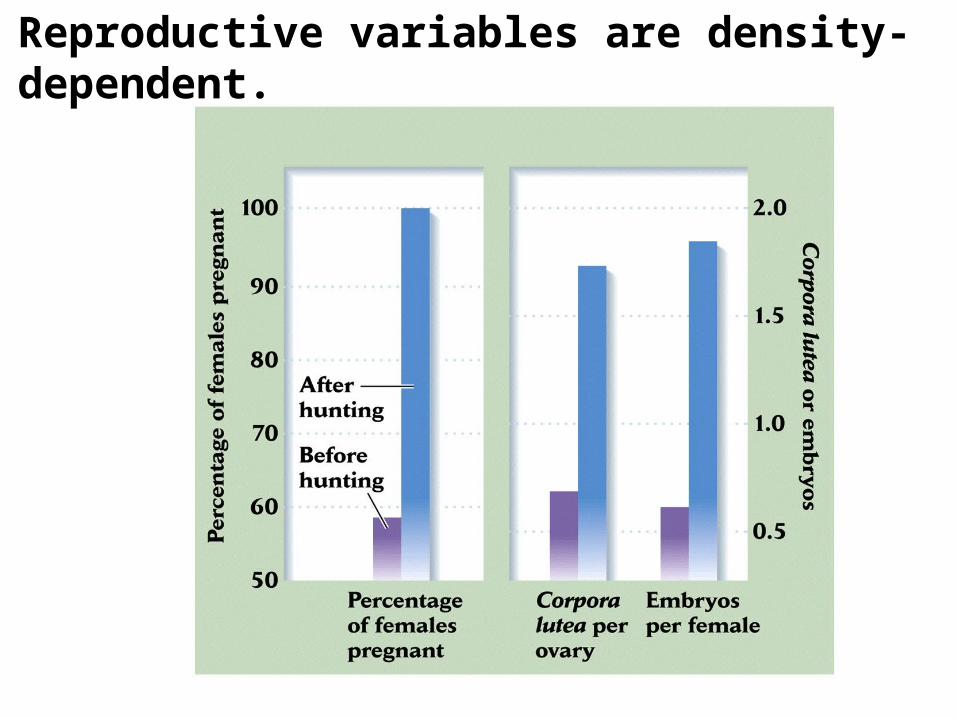
Reproductive variables are density-dependent.
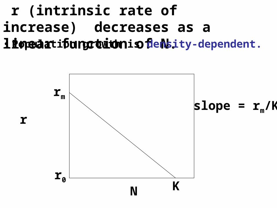
r (intrinsic rate of increase) decreases as a linear function of N.• Population growth is density-dependent.
rm
r
r0
N K
slope = rm/K
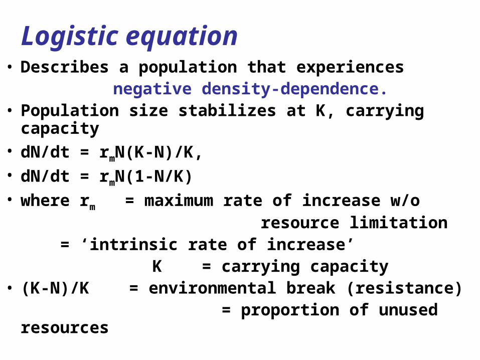
• Describes a population that experiences negative density-dependence.• Population size stabilizes at K, carrying capacity • dN/dt = rmN(K-N)/K,• dN/dt = rmN(1-N/K) • where rm = maximum rate of increase w/o resource limitation
= ‘intrinsic rate of increase’ K = carrying capacity • (K-N)/K = environmental break (resistance) = proportion of unused resources
Logistic equation
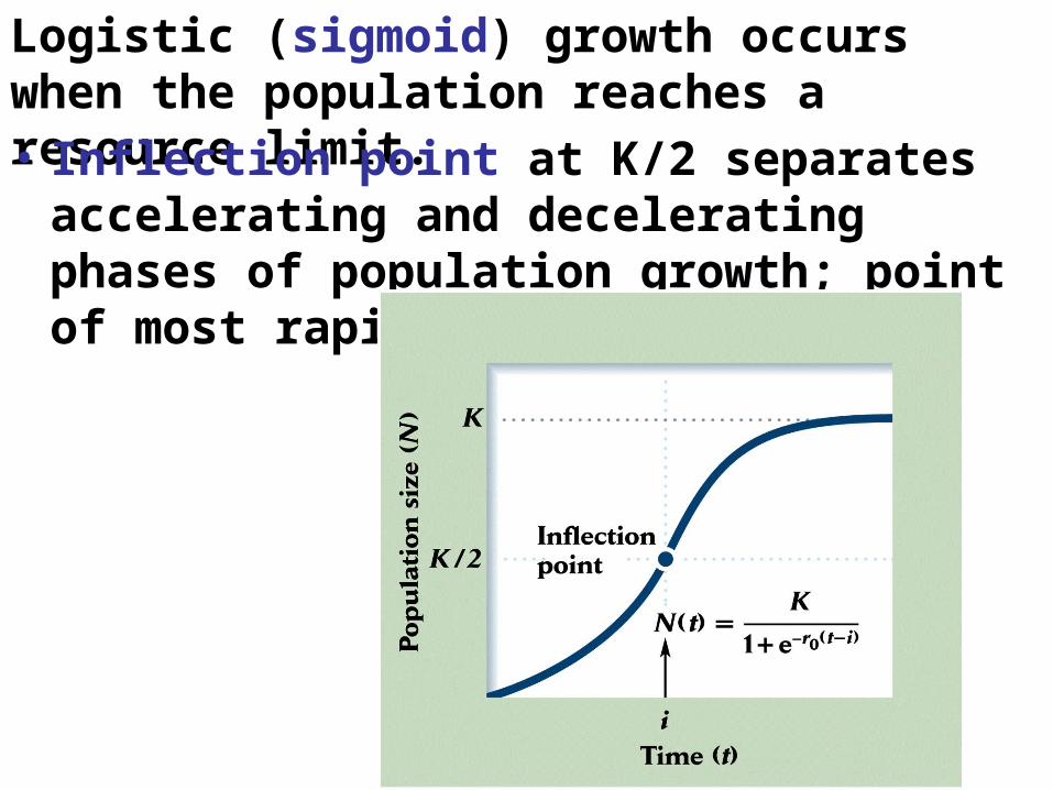
Logistic (sigmoid) growth occurs when the population reaches a resource limit.• Inflection point at K/2 separates
accelerating and decelerating phases of population growth; point of most rapid growth
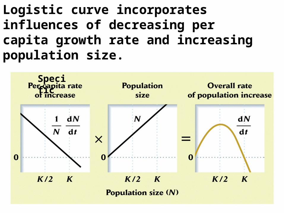
Logistic curve incorporates influences of decreasing per capita growth rate and increasing population size.
Specific
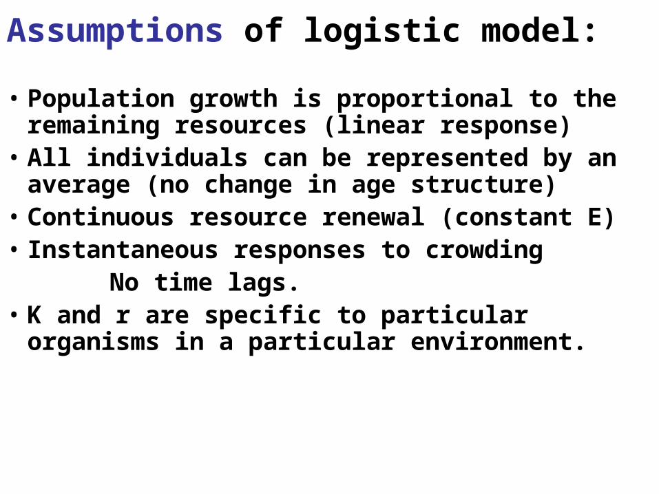
Assumptions of logistic model:
• Population growth is proportional to the remaining resources (linear response)
• All individuals can be represented by an average (no change in age structure)
• Continuous resource renewal (constant E)• Instantaneous responses to crowding No time lags.• K and r are specific to particular organisms
in a particular environment.
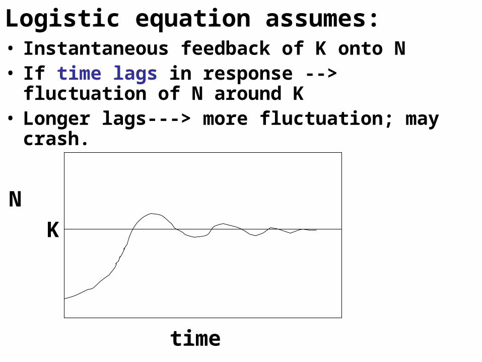
Logistic equation assumes:• Instantaneous feedback of K onto N• If time lags in response --> fluctuation of N
around K• Longer lags---> more fluctuation; may crash.
N
K
time
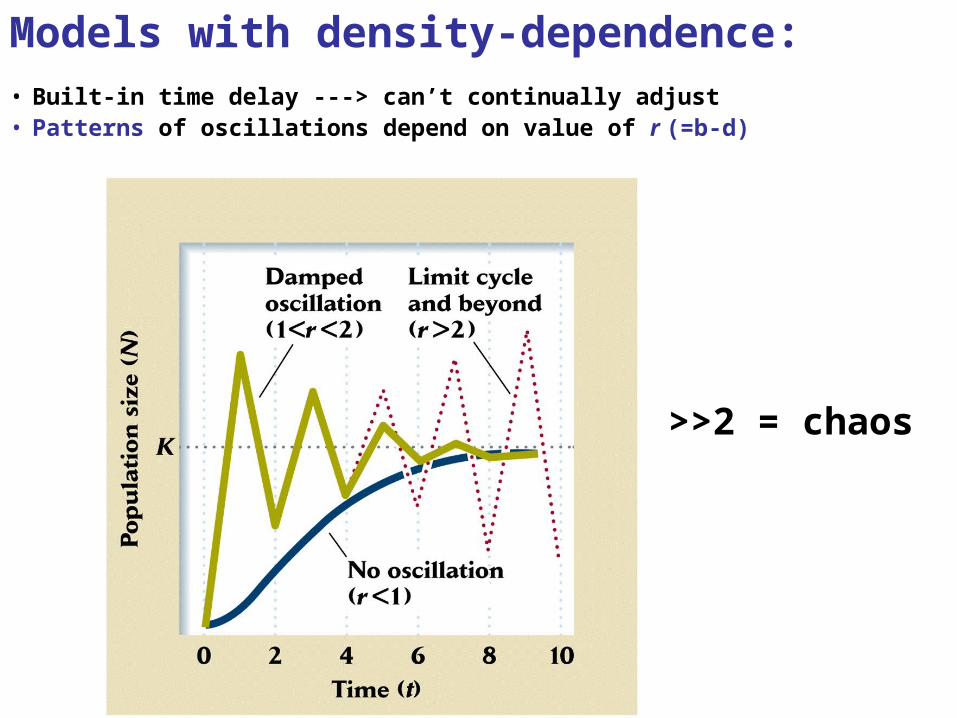
Models with density-dependence:• Built-in time delay ---> can’t continually adjust• Patterns of oscillations depend on value of r (=b-d)
>>2 = chaos
Density-dependent factors drive populations toward equilibrium (stable population size),
• BUT
• they also fluctuate around equilibrium due to:
• changes in environmental conditions
• chance
• intrinsic dynamics of population
responses
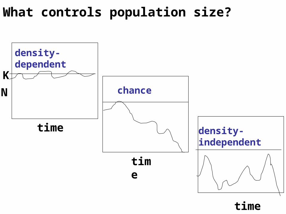
What controls population size?
time
time
time
N
density-dependent
chance
density-independent
K
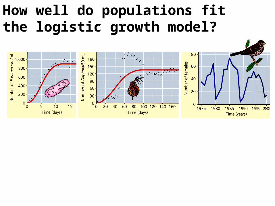
How well do populations fit the logistic growth model?
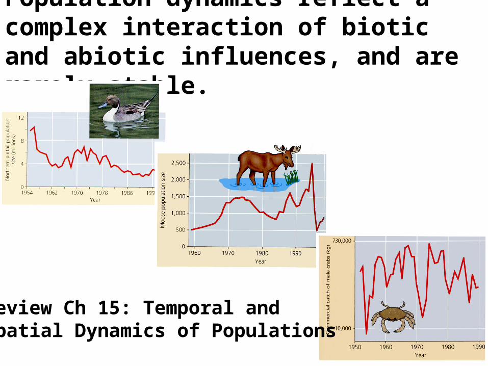
Population dynamics reflect a complex interaction of biotic and abiotic influences, and are rarely stable.
Review Ch 15: Temporal and Spatial Dynamics of Populations
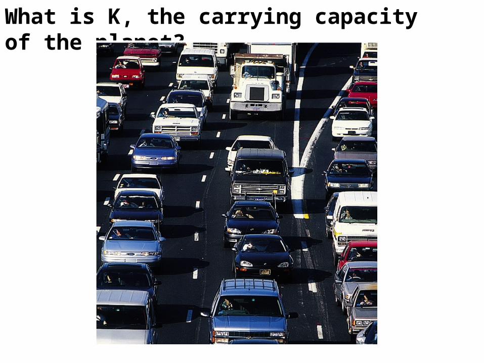
What is K, the carrying capacity of the planet?

Ecological footprints of some nations already exceed available ecological capacity.

Objectives• Review growth in unlimited environment• Geometric growth (seasonal reproduction)• Exponential growth (continuous reprod.)• Population Problems• Growth in limiting environment• Logistic model dN/dt = rN (K - N)/ K• Density-dependent birth and death rates• Assumptions of model• Reality of models
Vocabulary
Chapter 14 Population Growth and Regulation demography exponential growth* geometric growth per capita age structures* stable age distribution life tables fecundity survival survivorship cohort life table static life table* intrinsic rate of increase* net reproductive rate generation time doubling time carrying capacity (K) logistic equation* inflection point density-dependent factors density-independent factors self-thinning curve -3/2 power law r max* arithmetic* geometric* survivorship curves* doubling time model assumptions time lag size hierarchy Leslie matrix projection matrix transition probabilities life cycle figure life expectancy little r lambda (