Embed Size (px)
Citation preview
This is an Open Access document downloaded from ORCA, Cardiff University's institutional
repository: http://orca.cf.ac.uk/66236/
This is the author’s version of a work that was submitted to / accepted for publication.
Citation for final published version:
Xiao, Yi, Wan, Liang, Leung, Chi-Sing, Lai, Yukun and Wong, Tien-Tsin 2013. Example-based
color transfer for gradient meshes. IEEE Transactions on Multimedia 15 (3) , pp. 549-560.
10.1109/TMM.2012.2233725 file
Publishers page: http://dx.doi.org/10.1109/TMM.2012.2233725
<http://dx.doi.org/10.1109/TMM.2012.2233725>
Please note:
Changes made as a result of publishing processes such as copy-editing, formatting and page
numbers may not be reflected in this version. For the definitive version of this publication, please
refer to the published source. You are advised to consult the publisher’s version if you wish to cite
this paper.
This version is being made available in accordance with publisher policies. See
http://orca.cf.ac.uk/policies.html for usage policies. Copyright and moral rights for publications
made available in ORCA are retained by the copyright holders.
ACCEPTED BY IEEE TRANSACTIONS ON MULTIMEDIA 1
Example-based Color Transfer for
Gradient MeshesYi Xiao, Liang Wan, Member, IEEE, Chi-Sing Leung, Member, IEEE,
Yu-Kun Lai, and Tien-Tsin Wong, Member, IEEE
Abstract—Editing a photo-realistic gradient mesh is a toughtask. Even only editing the colors of an existing gradientmesh can be exhaustive and time-consuming. To facilitateuser-friendly color editing, we develop an example-based colortransfer method for gradient meshes, which borrows the colorcharacteristics of an example image to a gradient mesh. Westart by exploiting the constraints of the gradient mesh, andaccordingly propose a linear-operator-based color transfer
framework. Our framework operates only on colors and colorgradients of the mesh points and preserves the topologicalstructure of the gradient mesh. Bearing the framework inmind, we build our approach on PCA-based color transfer.After relieving the color range problem, we incorporate afusion-based optimization scheme to improve color similaritybetween the reference image and the recolored gradient mesh.Finally, a multi-swatch transfer scheme is provided to enablemore user control. Our approach is simple, effective, andmuch faster than color transferring the rastered gradientmesh directly. The experimental results also show that ourmethod can generate pleasing recolored gradient meshes.
Index Terms—Gradient mesh, example-based color transfer,linear operator, PCA-based color transfer
I. INTRODUCTION
GRadient mesh is a powerful vector graphics rep-
resentation offered by Adobe Illustrator and Corel
Coreldraw. Since it is suited to represent multi-colored
objects with smoothly varying colors, many artists use
gradient meshes to create photo-realistic vector arts. Based
on gradient meshes, image objects are represented by one
or more planar quad meshes, each forming a regularly
connected grid. Every grid point has the position, color,
and gradients of these quantities specified. The image rep-
resented by gradient meshes is then determined by bicubic
interpolation of these specified grid information.
A photo-realistic gradient mesh is not easy to be created
manually. It usually takes several hours even days to create
a gradient mesh, because artists have to manually edit the
attributes of each grid point. Even for a small gradient
Copyright (c) 2010 IEEE. Personal use of this material is per-mitted. However, permission to use this material for any other pur-poses must be obtained from the IEEE by sending a request to [email protected]. Xiao and C.S. Leung are with the Department of Electronic En-
gineering, City University of Hong Kong, Hong Kong. E-mail: [email protected], [email protected]. Wan (corresponding author) is with the School of Computer Soft-
ware, Tianjin University. E-mail: [email protected]. Lai is with Cardiff University. E-mail: [email protected]. Wong is with The Chinese University of Hong Kong. E-mail:
mesh with hundreds of grid points, artists may need to
take thousands of editing actions, which is labor intensive.
To relieve this problem, several methods for automatic or
semi-automatic generation of gradient meshes from a raster
image [1], [2] have been developed. Good results can be
obtained with the aid of some user assistances. However,
how to efficiently edit the attributes of gradient meshes is
still an open problem.
In this paper, we apply the idea of color transfer to
gradient meshes. Specifically, we let users change color
appearance of gradient meshes by referring to an example
image. Our application is analogous to color transfer on
images. But it should be pointed out that a gradient mesh
has particular constraints rather than an image. Firstly,
a grid point in a gradient mesh not only has color as
a pixel does in an image, but also has color gradients
defined in parametric domain. Secondly, gradient meshes
have grid structures which may be obtained via labor-
intensive manual creation and should be maintained during
the transfer.
We start our work by analytically investigating the effect
of linear operator on colors and color gradients of gradient
meshes. Based on our findings, a linear-operator-based
color transfer framework is proposed, which allows us
to perform color transfer on grid points only. Thanks to
the framework, we are able to build our approach on
a simple linear color transfer operator, i.e, PCA-based
transfer [3]. We then apply an extended PCA-based transfer
to handle the color range, and propose a minimization
scheme to generate color characteristics more similar to that
of the reference image. Afterwards, a gradient-preserving
algorithm is optionally performed to suppress local color
inconsistency. Finally, we develop a multi-swatch transfer
scheme to provide more user control on color appearance.
An example with two mesh objects is shown in Figure 1.
The main contribution of our work is a feasible color
transfer method that highly exploits the constraints of
gradient meshes. Our method is quite simple, parameter-
free and requires less user interventions. The only user input
is to ask users to specify color swatches. Given an example
image, our method is able to produce convincing recolored
gradient meshes. Note that our approach is performed on
the mesh grids directly. As a result, we can not only
maintain the grid structure of gradient meshes, but also
achieve fast performance due to the small size of mesh
objects.
2 ACCEPTED BY IEEE TRANSACTIONS ON MULTIMEDIA
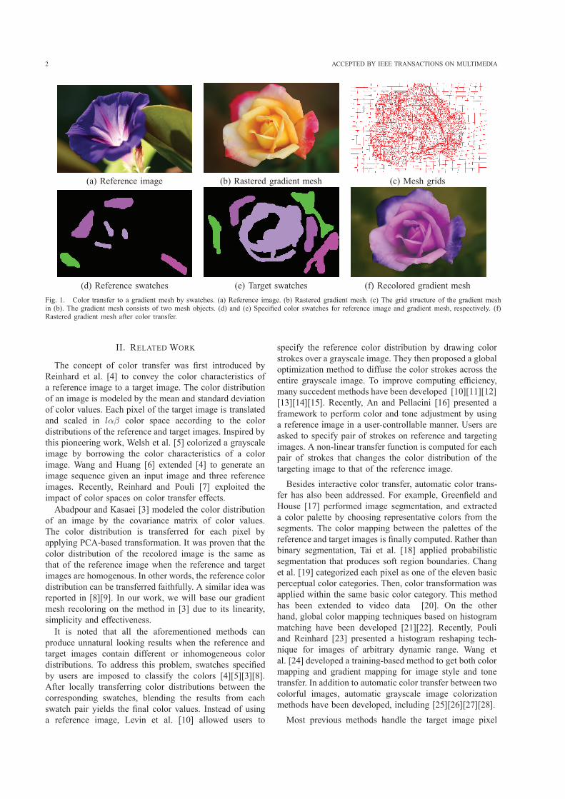
(a) Reference image (b) Rastered gradient mesh (c) Mesh grids
(d) Reference swatches (e) Target swatches (f) Recolored gradient mesh
Fig. 1. Color transfer to a gradient mesh by swatches. (a) Reference image. (b) Rastered gradient mesh. (c) The grid structure of the gradient meshin (b). The gradient mesh consists of two mesh objects. (d) and (e) Specified color swatches for reference image and gradient mesh, respectively. (f)Rastered gradient mesh after color transfer.
II. RELATED WORK
The concept of color transfer was first introduced by
Reinhard et al. [4] to convey the color characteristics of
a reference image to a target image. The color distribution
of an image is modeled by the mean and standard deviation
of color values. Each pixel of the target image is translated
and scaled in lαβ color space according to the color
distributions of the reference and target images. Inspired by
this pioneering work, Welsh et al. [5] colorized a grayscale
image by borrowing the color characteristics of a color
image. Wang and Huang [6] extended [4] to generate an
image sequence given an input image and three reference
images. Recently, Reinhard and Pouli [7] exploited the
impact of color spaces on color transfer effects.
Abadpour and Kasaei [3] modeled the color distribution
of an image by the covariance matrix of color values.
The color distribution is transferred for each pixel by
applying PCA-based transformation. It was proven that the
color distribution of the recolored image is the same as
that of the reference image when the reference and target
images are homogenous. In other words, the reference color
distribution can be transferred faithfully. A similar idea was
reported in [8][9]. In our work, we will base our gradient
mesh recoloring on the method in [3] due to its linearity,
simplicity and effectiveness.
It is noted that all the aforementioned methods can
produce unnatural looking results when the reference and
target images contain different or inhomogeneous color
distributions. To address this problem, swatches specified
by users are imposed to classify the colors [4][5][3][8].
After locally transferring color distributions between the
corresponding swatches, blending the results from each
swatch pair yields the final color values. Instead of using
a reference image, Levin et al. [10] allowed users to
specify the reference color distribution by drawing color
strokes over a grayscale image. They then proposed a global
optimization method to diffuse the color strokes across the
entire grayscale image. To improve computing efficiency,
many succedent methods have been developed [10][11][12]
[13][14][15]. Recently, An and Pellacini [16] presented a
framework to perform color and tone adjustment by using
a reference image in a user-controllable manner. Users are
asked to specify pair of strokes on reference and targeting
images. A non-linear transfer function is computed for each
pair of strokes that changes the color distribution of the
targeting image to that of the reference image.
Besides interactive color transfer, automatic color trans-
fer has also been addressed. For example, Greenfield and
House [17] performed image segmentation, and extracted
a color palette by choosing representative colors from the
segments. The color mapping between the palettes of the
reference and target images is finally computed. Rather than
binary segmentation, Tai et al. [18] applied probabilistic
segmentation that produces soft region boundaries. Chang
et al. [19] categorized each pixel as one of the eleven basic
perceptual color categories. Then, color transformation was
applied within the same basic color category. This method
has been extended to video data [20]. On the other
hand, global color mapping techniques based on histogram
matching have been developed [21][22]. Recently, Pouli
and Reinhard [23] presented a histogram reshaping tech-
nique for images of arbitrary dynamic range. Wang et
al. [24] developed a training-based method to get both color
mapping and gradient mapping for image style and tone
transfer. In addition to automatic color transfer between two
colorful images, automatic grayscale image colorization
methods have been developed, including [25][26][27][28].
Most previous methods handle the target image pixel
XIAO et al. 3
by pixel, and may produce spatially inconsistent artifacts.
To avoid such artifacts, Xiao and Ma [29] suggested
maintaining the fidelity of the target image, i.e., preserv-
ing the original gradients. The similar idea can also be
found in [30], [31], [32], although expressed in different
formulas. As later demonstrated in our paper, we apply a
gradient-preserving technique to reduce artifacts due to the
minimization scheme for color transfer.
III. COLOR TRANSFER FOR GRADIENT MESHES
In this section, we first describe the mathematical repre-
sentation of gradient meshes. Next, we discuss the linear-
operator-based color transfer framework. Afterwards, the
color transfer with single color swatch is presented in detail.
Finally, the color transfer with multiple color swatches is
introduced.
A. Gradient Mesh
A gradient mesh, as defined in [1][2], is a regularly
connected 2D grid. The primitive component of a gradient
mesh is a Ferguson patch [33], which is determined by
four nearby control points. Each control point specifies
three types of information, including position x, y, colorr, g, b and their gradients mu,mv, αmu, βmv, wherem is a component of either position or color. The gradients
mu and αmu (mv and βmv) share the same direction,
maintaining continuity between neighboring patches. A Fer-
guson patch is evaluated via bicubic Hermite interpolation,
given by
m(u, v) = uCQCTvT , (1)
where
Q =
⎡
⎢
⎢
⎣
m0 m2 m0v m2
v
m1 m3 m1v m3
v
m0u m2
u 0 0m1
u m3u 0 0
⎤
⎥
⎥
⎦
, C =
⎡
⎢
⎢
⎣
1 0 0 00 0 1 0−3 3 −2 −12 −2 1 1
⎤
⎥
⎥
⎦
,
the upper script ofm indicates one of the four control points
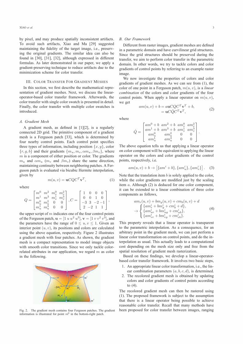
of the Ferguson patch, u = [1 u u2 u3], v = [1 v v2 v3], andthe parameters have the range of 0 ≤ u, v ≤ 1. Given aninterior point (u, v), its positions and colors are calculatedusing the above equation, respectively. Figure 2 illustrates
a gradient mesh with four patches. As shown, the gradient
mesh is a compact representation to model image objects
with smooth color transitions. Since we only tackle color-
related attributes in our application, we regard m as color
in the following.
um
vm
0m
1m
2m
3m
vm
um
Fig. 2. The gradient mesh contains four Ferguson patches. The gradientinformation is illustrated for point m0 in the bottom-right patch.
B. Our Framework
Different from raster images, gradient meshes are defined
in a parametric domain and have curvilinear grid structures.
Since the grid structures should be preserved during the
transfer, we aim to perform color transfer in the parametric
domain. In other words, we try to tackle colors and color
gradients of control points by referring to an example raster
image.
We now investigate the properties of colors and color
gradients of gradient meshes. As we can see from (1), the
color of one point in a Ferguson patch, m(u, v), is a linearcombination of the colors and color gradients of the four
control points. When apply a linear operator on m(u, v),we get
am(u, v) + b = auCQCTvT + b,
= uCQCTvT ,
(2)
where
Q =
⎡
⎢
⎢
⎣
am0 + b am2 + b am0v am2
v
am1 + b am3 + b am1v am3
v
am0u am2
u 0 0am1
u am3u 0 0
⎤
⎥
⎥
⎦
.
The above equation tells us that applying a linear operator
on color component will be equivalent to applying the linear
operator on the colors and color gradients of the control
points, respectively, i.e.
am(u, v) + b →[
ami + b, amiu, am
iv]
. (3)
Note that the translation item b is solely applied to the color,while the color gradients are modified just by the scaling
item a. Although (2) is deduced for one color component,it can be extended to a linear combination of three color
components as follows,
amr(u, v) + bmg(u, v) + cmb(u, v) + d
→
⎧
⎨
⎩
amir + bmi
g + cmib + d,
amiur + bmi
ug + cmiub,
amivr + bmi
vg + cmivb.
(4)
This property reveals that a linear operator is transparent
to the parametric interpolation. As a consequence, for an
arbitrary point in the gradient mesh, we can just perform a
linear color transformation on control points, and do the in-
terpolation as usual. This actually leads to a computational
cost depending on the mesh size only and free from the
spatial resolution of gradient mesh rasterization.
Based on these findings, we develop a linear-operator-
based color transfer framework. It involves two basic steps,
1. An appropriate linear color transformation, i.e., the lin-
ear combination parameters (a, b, c, d), is determined.2. The recolored gradient mesh is obtained by updating
colors and color gradients of control points according
to (4).
The recolored gradient mesh can then be rastered using
(1). The proposed framework is subject to the assumption
that there is a linear operator being possible to achieve
reasonable color transfer. Recall that many methods have
been proposed for color transfer between images, ranging
4 ACCEPTED BY IEEE TRANSACTIONS ON MULTIMEDIA
from simple linear operator [5][3][8] to much complicated
algorithms [20][26][21][15]. On the other hand, gradient
meshes are usually not used to represent natural images
with complex scenes. Therefore, we can safely rely on sim-
ple yet efficient color transfer methods. To be more specific,
we will base our work on PCA-based transformation [3].
C. Single-Swatch Color Transfer
The basic idea of PCA-based color transfer is to estimate
the color characteristics by covariance matrix of colors,
and convert colors from the target into the reference color
distribution via principal component analysis (PCA). How-
ever, using the colors of mesh points alone cannot yield
an accurate estimation of color statistics of the gradient
mesh. It is also infeasible to compute the covariance matrix
analytically. As we always have a raster image It fromgradient meshes for preview, we can estimate the color
mapping between It and the reference image Ir .1) PCA-based Color Transfer Without Scaling: Let Mt
and Mr denote the covariance matrices of It and Ir inRGB color space (other color spaces are also applicable).
PCA can be done by eigenvalue decomposition of covari-
ance matrix as follows,
M = U · Σ · U−1. (5)
where U is an orthogonal matrice composed of eigenvectorsof M , Σ = diag(λR, λG, λB) containing the eigenvaluesof M . Then the PCA of Mt and Mr gives the orthogonal
matrices Ut and Ur. For the color vector ct of a controlpoint, PCA-based color transfer [3] computes the recolored
vector c as
c = UrU−1
t (ct − ηt) + ηr, (6)
where ηt, ηr are the mean color vectors of It and Ir.Recall that in addition to colors, our linear-operator-
based transfer framework also modifies color gradients.
According to (4), the recolored gradient vector of the
control point, ∂c, is computed as
∂c = UrU−1
t ∂ct, (7)
where ∂ct denotes 3-dimensional color gradient vectors ineither u or v direction. Note that each control point has twogradient vectors and both of them should be transformed.
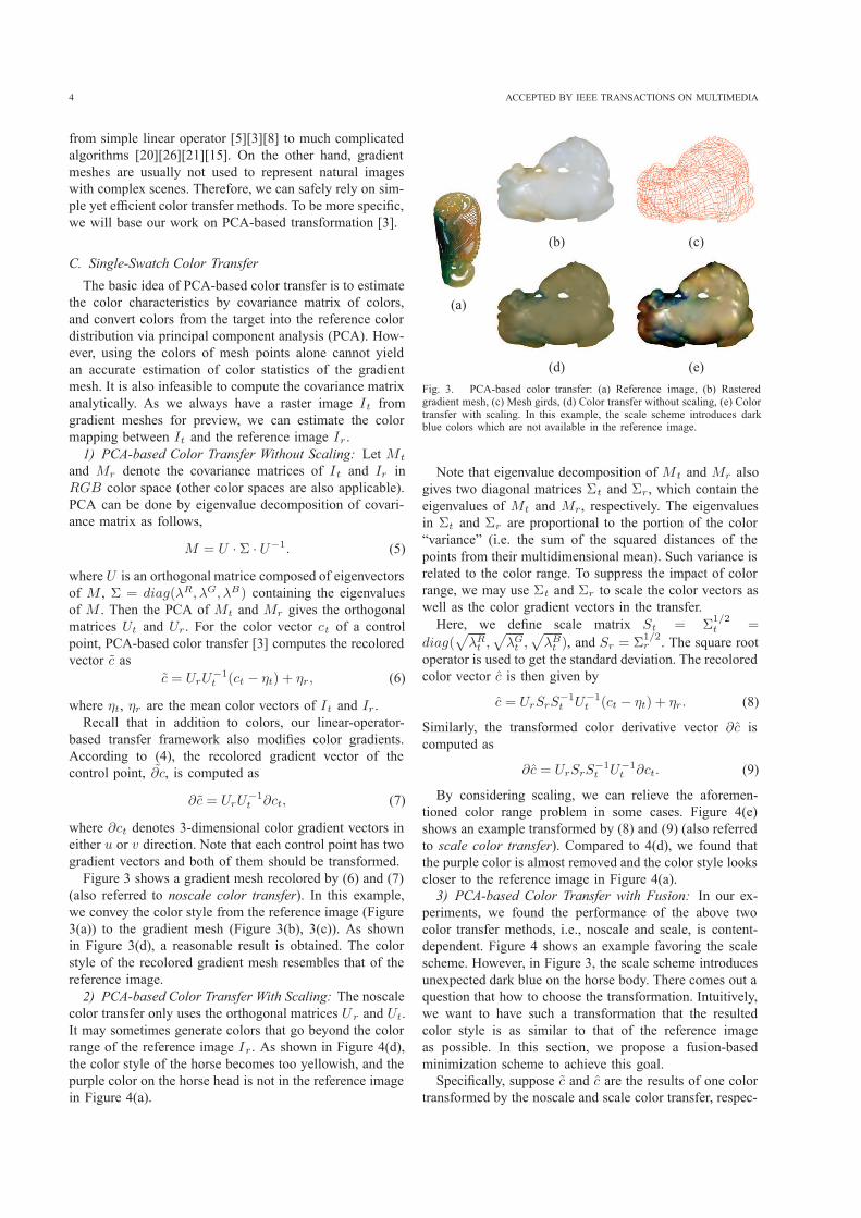
Figure 3 shows a gradient mesh recolored by (6) and (7)
(also referred to noscale color transfer). In this example,
we convey the color style from the reference image (Figure
3(a)) to the gradient mesh (Figure 3(b), 3(c)). As shown
in Figure 3(d), a reasonable result is obtained. The color
style of the recolored gradient mesh resembles that of the
reference image.
2) PCA-based Color Transfer With Scaling: The noscale
color transfer only uses the orthogonal matrices Ur and Ut.
It may sometimes generate colors that go beyond the color
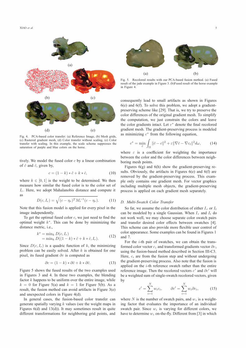
range of the reference image Ir. As shown in Figure 4(d),the color style of the horse becomes too yellowish, and the
purple color on the horse head is not in the reference image
in Figure 4(a).
(a)
(b) (c)
(d) (e)
Fig. 3. PCA-based color transfer: (a) Reference image, (b) Rasteredgradient mesh, (c) Mesh girds, (d) Color transfer without scaling, (e) Colortransfer with scaling. In this example, the scale scheme introduces darkblue colors which are not available in the reference image.
Note that eigenvalue decomposition of M t and Mr also
gives two diagonal matrices Σt and Σr, which contain the
eigenvalues of Mt and Mr, respectively. The eigenvalues
in Σt and Σr are proportional to the portion of the color
“variance” (i.e. the sum of the squared distances of the
points from their multidimensional mean). Such variance is
related to the color range. To suppress the impact of color
range, we may use Σt and Σr to scale the color vectors as
well as the color gradient vectors in the transfer.
Here, we define scale matrix St = Σ1/2t =
diag(√
λRt ,
√
λGt ,
√
λBt ), and Sr = Σ
1/2r . The square root
operator is used to get the standard deviation. The recolored
color vector c is then given by
c = UrSrS−1
t U−1
t (ct − ηt) + ηr. (8)
Similarly, the transformed color derivative vector ∂c iscomputed as
∂c = UrSrS−1
t U−1
t ∂ct. (9)
By considering scaling, we can relieve the aforemen-
tioned color range problem in some cases. Figure 4(e)
shows an example transformed by (8) and (9) (also referred
to scale color transfer). Compared to 4(d), we found that
the purple color is almost removed and the color style looks
closer to the reference image in Figure 4(a).
3) PCA-based Color Transfer with Fusion: In our ex-
periments, we found the performance of the above two
color transfer methods, i.e., noscale and scale, is content-
dependent. Figure 4 shows an example favoring the scale
scheme. However, in Figure 3, the scale scheme introduces
unexpected dark blue on the horse body. There comes out a
question that how to choose the transformation. Intuitively,
we want to have such a transformation that the resulted
color style is as similar to that of the reference image
as possible. In this section, we propose a fusion-based
minimization scheme to achieve this goal.
Specifically, suppose c and c are the results of one colortransformed by the noscale and scale color transfer, respec-
XIAO et al. 5
(a)
(b) (c)
(d) (e)
Fig. 4. PCA-based color transfer: (a) Reference Image, (b) Mesh grids,(c) Rastered gradient mesh, (d) Color transfer without scaling, (e) Colortransfer with scaling. In this example, the scale scheme suppresses thesaturation of purple and blue colors on the horse.
tively. We model the fused color c by a linear combinationof c and c, given by,
c = (1 − k) ∗ c+ k ∗ c, (10)
where k ∈ [0, 1] is the weight to be determined. We thenmeasure how similar the fused color is to the color set of
Ir. Here, we adopt Mahalanobis distance and compute itas
D(c, Ir) =
√
(c− ηr)TM−1r (c− ηr). (11)
Note that this fusion model is applied for every pixel in the
image independently.
To get the optimal fused color c, we just need to find theoptimal weight k∗. This can be done by minimizing the
distance metric, i.e.,
k∗ = mink D(c, Ir)= mink D((1− k) ∗ c+ k ∗ c, Ir).
(12)
Since D(c, Ir) is a quadric function of k, the minimizingproblem can be easily solved. After k is obtained for onepixel, its fused gradient ∂c is computed as
∂c = (1− k) ∗ ∂c+ k ∗ ∂c. (13)
Figure 5 shows the fused results of the two examples used
in Figures 3 and 4. In these two examples, the blending
factor k happens to be uniform over the entire image, whilek = 0 for Figure 5(a) and k = 1 for Figure 5(b). As aresult, the fusion method can avoid artifacts in Figure 3(e)
and unexpected colors in Figure 4(d).
In general cases, the fusion-based color transfer can
generate spatially varying k values (see the weight maps inFigures 6(d) and 13(d)). It may sometimes result in quite
different transformations for neighboring grid points, and
(a) (b)
Fig. 5. Recolored results with our PCA-based fusion method. (a) Fusedresult of the jade example in Figure 3. (b)Fused result of the horse examplein Figure 4.
consequently lead to small artifacts as shown in Figures
6(e) and 6(f). To solve this problem, we adopt a gradient-
preserving scheme like [29]. That is, we try to preserve the
color differences of the original gradient mesh. To simplify
the computation, we just constrain the colors and leave
the color gradients intact. Let c∗ denote the final recoloredgradient mesh. The gradient-preserving process is modeled
as minimizing c∗ from the following equation,
c∗ = minc
∫
Ω
‖c− c‖2 + ε‖∇c−∇ct‖2dω, (14)
where ε is a coefficient for weighting the importancebetween the color and the color differences between neigh-
boring mesh points.
Figures 6(g) and 6(h) show the gradient-preserving re-
sults. Obviously, the artifacts in Figures 6(e) and 6(f) are
removed by the gradient-preserving process. This exam-
ple only contains one gradient mesh. For vector graphics
including multiple mesh objects, the gradient-preserving
process is applied on each gradient mesh separately.
D. Multi-Swatch Color Transfer
So far, we assume the color distribution of either Ir or Itcan be modeled by a single Gaussian. When Ir and It donot work well, we may choose separate color swatch pairs
and transfer desired color effects between swatches [4].
This scheme can also provide more flexible user control of
color appearance. Some examples can be found in Figures 1
and 7.
For the i-th pair of swatches, we can obtain the trans-formed color vector ci and transformed gradients vector ∂c iusing the fusion-based method described in Section III-C3.
Here, ci are from the fusion step and without undergoingthe gradient-preserving process. Also note that the fusion is
applied on the i-th reference swatch rather than the entirereference image. Then the recolored vectors c ′ and ∂c′ willbe a weighted sum of single-swatch recolored vectors, given
by
c′ =
N∑
i=1
wici, ∂c′ =
N∑
i=1
wi∂ci, (15)
where N is the number of swatch pairs, and wi is a weight-
ing factor that evaluates the importance of an individual
swatch pair. Since wi is varying for different colors, we
have to determine wi on-the-fly. Different from [3] in which
6 ACCEPTED BY IEEE TRANSACTIONS ON MULTIMEDIA
(a) (b) (c) (d)
(e) (f) (g) (h)
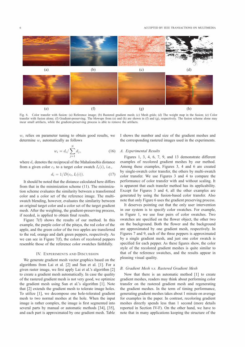
Fig. 6. Color transfer with fusion: (a) Reference image; (b) Rastered gradient mesh; (c) Mesh grids; (d) The weight map in the fusion; (e) Colortransfer with fusion alone; (f) Gradient-preserving; The blowups from (e) and (h) are shown in (f) and (g), respectively. The fusion scheme alone mayincur small artifacts, while the gradient-preserving process is able to remove the artifacts.
wi relies on parameter tuning to obtain good results, we
determine wi automatically as follows
wi = di/
N∑
j=1
dj , (16)
where di denotes the reciprocal of the Mahalonobis distancefrom a given color ct to a target color swatch It(i), i.e.,
di = 1/D(ct, It(i)). (17)
It should be noted that the distance calculated here differs
from that in the minimization scheme (11). The minimiza-
tion scheme evaluates the similarity between a transformed
color and a color set of the reference image. The multi-
swatch blending, however, evaluates the similarity between
an original target color and a color set of the target gradient
mesh. After the weighting, the gradient-preserving process,
if needed, is applied to obtain final results.
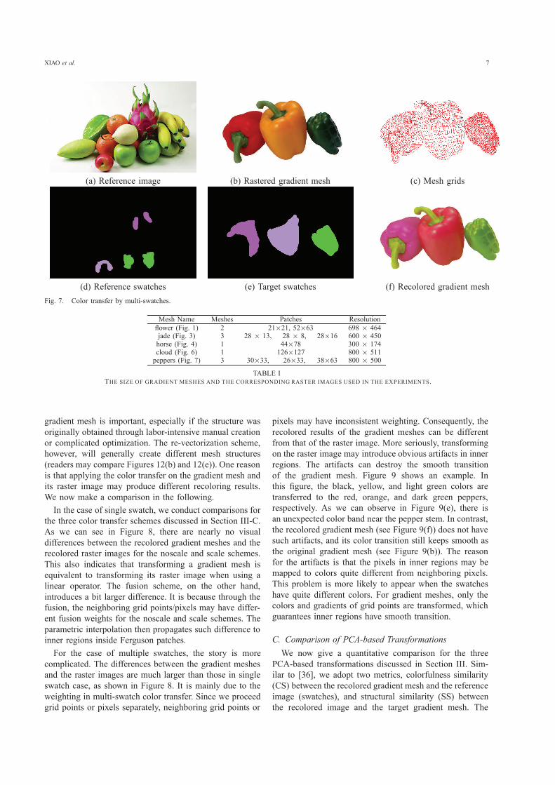
Figure 7(f) shows the results of our method. In this
example, the purple color of the pitaya, the red color of the
apple, and the green color of the two apples are transferred
to the red, orange and dark green peppers, respectively. As
we can see in Figure 7(f), the colors of recolored peppers
resemble those of the reference color swatches faithfully.
IV. EXPERIMENTS AND DISCUSSION
We generate gradient mesh vector graphics based on the
algorithms from Lai et al. [2] and Sun et al. [1]. For a
given raster image, we first apply Lai et al.’s algorithm [2]
to create a gradient mesh automatically. In case the quality
of the rastered gradient mesh is not very good, we optimize
the gradient mesh using Sun et al.’s algorithm [1]. Note
that [2] extends the gradient mesh to tolerate image holes.
To utilize [1], we decompose one hole-tolerated gradient
mesh to two normal meshes at the hole. When the input
image is rather complex, the image is first segmented into
several parts by manual or automatic methods [34], [35],
and each part is approximated by one gradient mesh. Table
I shows the number and size of the gradient meshes and
the corresponding rastered images used in the experiments.
A. Experimental Results
Figures 1, 3, 4, 6, 7, 9, and 13 demonstrate different
examples of recolored gradient meshes by our method.
Among these examples, Figures 3, 4 and 6 are created
by single-swatch color transfer, the others by multi-swatch
color transfer. We use Figures 3 and 4 to compare the
performance of color transfer with and without scaling. It
is apparent that each transfer method has its applicability.
Except for Figures 3 and 4, all the other examples are
generated by using the fusion-based color transfer. Also
note that only Figure 6 uses the gradient preserving process.
It deserves pointing out that the only user intervention
in our system is to specify color swatches. For example,
in Figure 1, we use four pairs of color swatches. Two
swatches are specified on the flower object, the other two
on the background. Both the flower and the background
are approximated by one gradient mesh, respectively. In
Figures 7 and 9, each of the three peppers is approximated
by a single gradient mesh, and just one color swatch is
specified for each pepper. As these figures show, the color
style of the recolored gradient meshes is quite similar to
that of the reference swatches, and the results appear in
pleasing visual quality.
B. Gradient Mesh v.s. Rastered Gradient Mesh
Now that there is an automatic method [1] to create
gradient meshes, readers may think about performing color
transfer on the rastered gradient mesh and regenerating
the gradient meshes. In the term of timing performance,
generating gradient meshes takes about 1 minute on average
for examples in the paper. In contrast, recoloring gradient
meshes directly spends less than 1 second (more details
reported in Section IV-F). On the other hand, we have to
note that in many applications keeping the structure of the
XIAO et al. 7
(a) Reference image (b) Rastered gradient mesh (c) Mesh grids
(d) Reference swatches (e) Target swatches (f) Recolored gradient mesh
Fig. 7. Color transfer by multi-swatches.
Mesh Name Meshes Patches Resolution
flower (Fig. 1) 2 21×21, 52×63 698 × 464jade (Fig. 3) 3 28 × 13, 28 × 8, 28×16 600 × 450horse (Fig. 4) 1 44×78 300 × 174cloud (Fig. 6) 1 126×127 800 × 511peppers (Fig. 7) 3 30×33, 26×33, 38×63 800 × 500
TABLE ITHE SIZE OF GRADIENT MESHES AND THE CORRESPONDING RASTER IMAGES USED IN THE EXPERIMENTS.
gradient mesh is important, especially if the structure was
originally obtained through labor-intensive manual creation
or complicated optimization. The re-vectorization scheme,
however, will generally create different mesh structures
(readers may compare Figures 12(b) and 12(e)). One reason
is that applying the color transfer on the gradient mesh and
its raster image may produce different recoloring results.
We now make a comparison in the following.
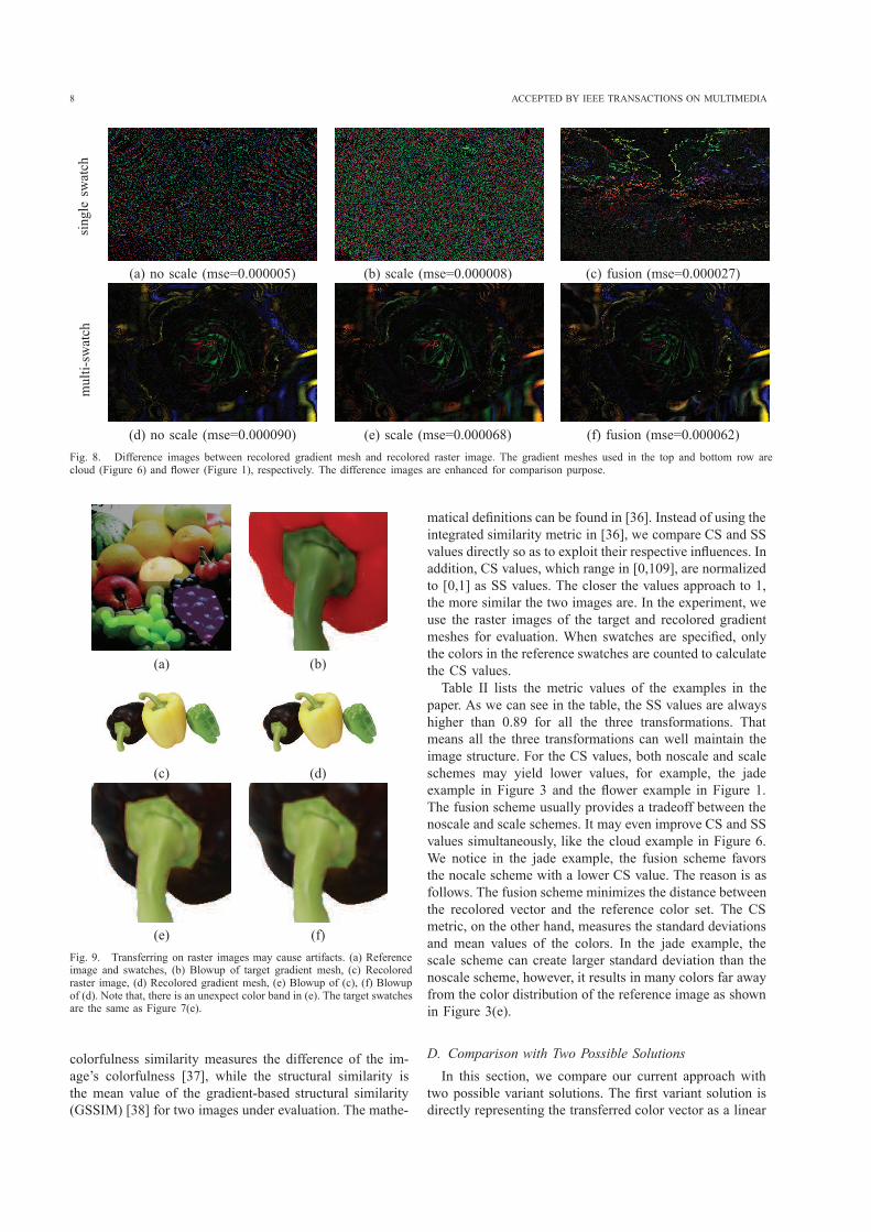
In the case of single swatch, we conduct comparisons for
the three color transfer schemes discussed in Section III-C.
As we can see in Figure 8, there are nearly no visual
differences between the recolored gradient meshes and the
recolored raster images for the noscale and scale schemes.
This also indicates that transforming a gradient mesh is
equivalent to transforming its raster image when using a
linear operator. The fusion scheme, on the other hand,
introduces a bit larger difference. It is because through the
fusion, the neighboring grid points/pixels may have differ-
ent fusion weights for the noscale and scale schemes. The
parametric interpolation then propagates such difference to
inner regions inside Ferguson patches.
For the case of multiple swatches, the story is more
complicated. The differences between the gradient meshes
and the raster images are much larger than those in single
swatch case, as shown in Figure 8. It is mainly due to the
weighting in multi-swatch color transfer. Since we proceed
grid points or pixels separately, neighboring grid points or
pixels may have inconsistent weighting. Consequently, the
recolored results of the gradient meshes can be different
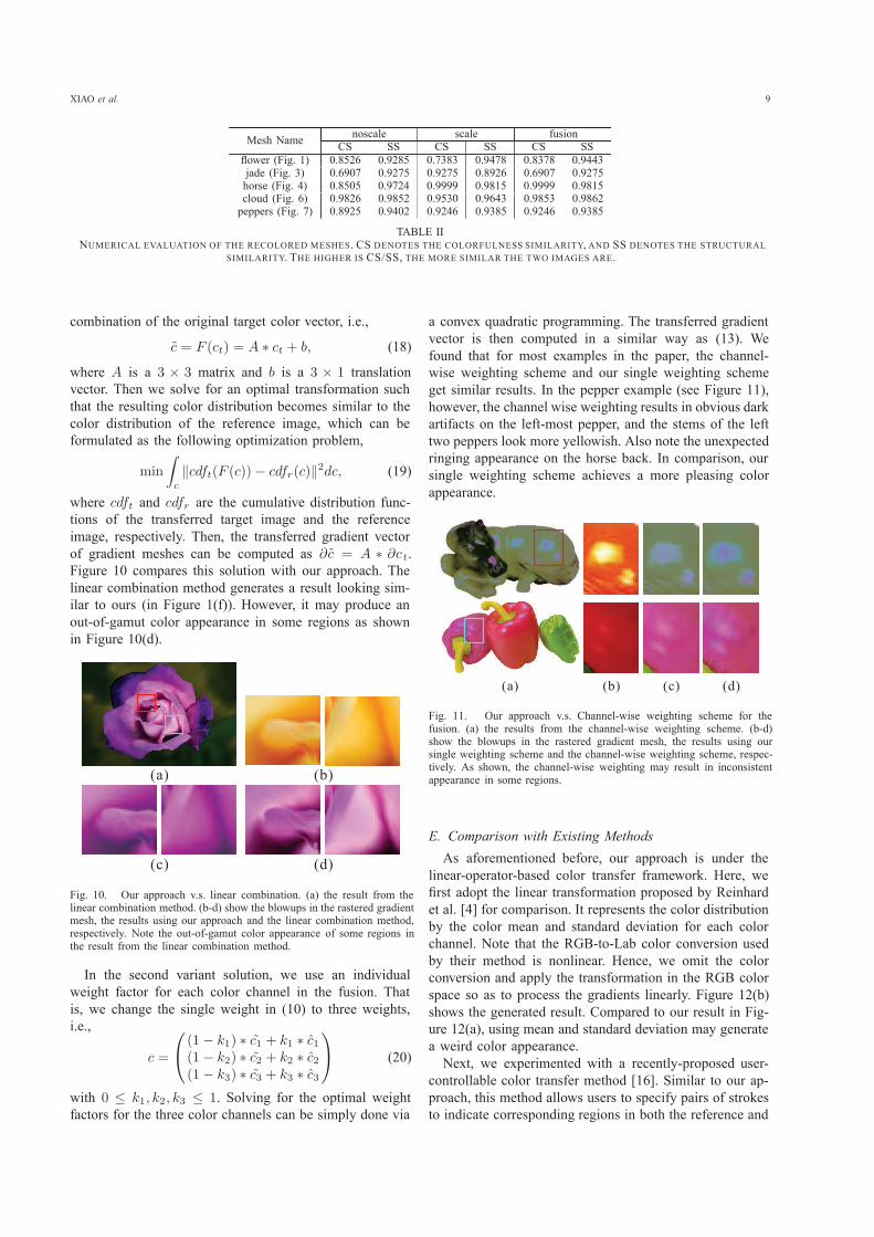
from that of the raster image. More seriously, transforming
on the raster image may introduce obvious artifacts in inner
regions. The artifacts can destroy the smooth transition
of the gradient mesh. Figure 9 shows an example. In
this figure, the black, yellow, and light green colors are
transferred to the red, orange, and dark green peppers,
respectively. As we can observe in Figure 9(e), there is
an unexpected color band near the pepper stem. In contrast,
the recolored gradient mesh (see Figure 9(f)) does not have
such artifacts, and its color transition still keeps smooth as
the original gradient mesh (see Figure 9(b)). The reason
for the artifacts is that the pixels in inner regions may be
mapped to colors quite different from neighboring pixels.
This problem is more likely to appear when the swatches
have quite different colors. For gradient meshes, only the
colors and gradients of grid points are transformed, which
guarantees inner regions have smooth transition.
C. Comparison of PCA-based Transformations
We now give a quantitative comparison for the three
PCA-based transformations discussed in Section III. Sim-
ilar to [36], we adopt two metrics, colorfulness similarity
(CS) between the recolored gradient mesh and the reference
image (swatches), and structural similarity (SS) between
the recolored image and the target gradient mesh. The
8 ACCEPTED BY IEEE TRANSACTIONS ON MULTIMEDIA
singleswatch
(a) no scale (mse=0.000005) (b) scale (mse=0.000008) (c) fusion (mse=0.000027)
multi-swatch
(d) no scale (mse=0.000090) (e) scale (mse=0.000068) (f) fusion (mse=0.000062)
Fig. 8. Difference images between recolored gradient mesh and recolored raster image. The gradient meshes used in the top and bottom row arecloud (Figure 6) and flower (Figure 1), respectively. The difference images are enhanced for comparison purpose.
(a) (b)
(c) (d)
(e) (f)
Fig. 9. Transferring on raster images may cause artifacts. (a) Referenceimage and swatches, (b) Blowup of target gradient mesh, (c) Recoloredraster image, (d) Recolored gradient mesh, (e) Blowup of (c), (f) Blowupof (d). Note that, there is an unexpect color band in (e). The target swatchesare the same as Figure 7(e).
colorfulness similarity measures the difference of the im-
age’s colorfulness [37], while the structural similarity is
the mean value of the gradient-based structural similarity
(GSSIM) [38] for two images under evaluation. The mathe-
matical definitions can be found in [36]. Instead of using the
integrated similarity metric in [36], we compare CS and SS
values directly so as to exploit their respective influences. In
addition, CS values, which range in [0,109], are normalized
to [0,1] as SS values. The closer the values approach to 1,
the more similar the two images are. In the experiment, we
use the raster images of the target and recolored gradient
meshes for evaluation. When swatches are specified, only
the colors in the reference swatches are counted to calculate
the CS values.
Table II lists the metric values of the examples in the
paper. As we can see in the table, the SS values are always
higher than 0.89 for all the three transformations. That
means all the three transformations can well maintain the
image structure. For the CS values, both noscale and scale
schemes may yield lower values, for example, the jade
example in Figure 3 and the flower example in Figure 1.
The fusion scheme usually provides a tradeoff between the
noscale and scale schemes. It may even improve CS and SS
values simultaneously, like the cloud example in Figure 6.
We notice in the jade example, the fusion scheme favors
the nocale scheme with a lower CS value. The reason is as
follows. The fusion scheme minimizes the distance between
the recolored vector and the reference color set. The CS
metric, on the other hand, measures the standard deviations
and mean values of the colors. In the jade example, the
scale scheme can create larger standard deviation than the
noscale scheme, however, it results in many colors far away
from the color distribution of the reference image as shown
in Figure 3(e).
D. Comparison with Two Possible Solutions
In this section, we compare our current approach with
two possible variant solutions. The first variant solution is
directly representing the transferred color vector as a linear
XIAO et al. 9
Mesh Namenoscale scale fusion
CS SS CS SS CS SS
flower (Fig. 1) 0.8526 0.9285 0.7383 0.9478 0.8378 0.9443jade (Fig. 3) 0.6907 0.9275 0.9275 0.8926 0.6907 0.9275horse (Fig. 4) 0.8505 0.9724 0.9999 0.9815 0.9999 0.9815cloud (Fig. 6) 0.9826 0.9852 0.9530 0.9643 0.9853 0.9862peppers (Fig. 7) 0.8925 0.9402 0.9246 0.9385 0.9246 0.9385
TABLE IINUMERICAL EVALUATION OF THE RECOLORED MESHES. CS DENOTES THE COLORFULNESS SIMILARITY, AND SS DENOTES THE STRUCTURAL
SIMILARITY. THE HIGHER IS CS/SS, THE MORE SIMILAR THE TWO IMAGES ARE.
combination of the original target color vector, i.e.,
c = F (ct) = A ∗ ct + b, (18)
where A is a 3 × 3 matrix and b is a 3 × 1 translationvector. Then we solve for an optimal transformation such
that the resulting color distribution becomes similar to the
color distribution of the reference image, which can be
formulated as the following optimization problem,
min
∫
c
‖cdft(F (c))− cdfr(c)‖2dc, (19)
where cdft and cdfr are the cumulative distribution func-tions of the transferred target image and the reference
image, respectively. Then, the transferred gradient vector
of gradient meshes can be computed as ∂c = A ∗ ∂ct.Figure 10 compares this solution with our approach. The
linear combination method generates a result looking sim-
ilar to ours (in Figure 1(f)). However, it may produce an
out-of-gamut color appearance in some regions as shown
in Figure 10(d).
(a) (b)
(c) (d)
Fig. 10. Our approach v.s. linear combination. (a) the result from thelinear combination method. (b-d) show the blowups in the rastered gradientmesh, the results using our approach and the linear combination method,respectively. Note the out-of-gamut color appearance of some regions inthe result from the linear combination method.
In the second variant solution, we use an individual
weight factor for each color channel in the fusion. That
is, we change the single weight in (10) to three weights,
i.e.,
c =
⎛
⎝
(1− k1) ∗ c1 + k1 ∗ c1(1− k2) ∗ c2 + k2 ∗ c2(1− k3) ∗ c3 + k3 ∗ c3
⎞
⎠ (20)
with 0 ≤ k1, k2, k3 ≤ 1. Solving for the optimal weightfactors for the three color channels can be simply done via
a convex quadratic programming. The transferred gradient
vector is then computed in a similar way as (13). We
found that for most examples in the paper, the channel-
wise weighting scheme and our single weighting scheme
get similar results. In the pepper example (see Figure 11),
however, the channel wise weighting results in obvious dark
artifacts on the left-most pepper, and the stems of the left
two peppers look more yellowish. Also note the unexpected
ringing appearance on the horse back. In comparison, our
single weighting scheme achieves a more pleasing color
appearance.
(a) (b) (c) (d)
Fig. 11. Our approach v.s. Channel-wise weighting scheme for thefusion. (a) the results from the channel-wise weighting scheme. (b-d)show the blowups in the rastered gradient mesh, the results using oursingle weighting scheme and the channel-wise weighting scheme, respec-tively. As shown, the channel-wise weighting may result in inconsistentappearance in some regions.
E. Comparison with Existing Methods
As aforementioned before, our approach is under the
linear-operator-based color transfer framework. Here, we
first adopt the linear transformation proposed by Reinhard
et al. [4] for comparison. It represents the color distribution
by the color mean and standard deviation for each color
channel. Note that the RGB-to-Lab color conversion used
by their method is nonlinear. Hence, we omit the color
conversion and apply the transformation in the RGB color
space so as to process the gradients linearly. Figure 12(b)
shows the generated result. Compared to our result in Fig-
ure 12(a), using mean and standard deviation may generate
a weird color appearance.
Next, we experimented with a recently-proposed user-
controllable color transfer method [16]. Similar to our ap-
proach, this method allows users to specify pairs of strokes
to indicate corresponding regions in both the reference and
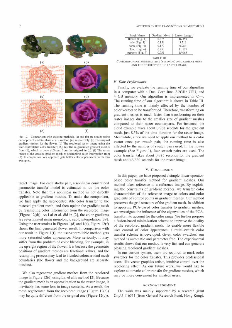
10 ACCEPTED BY IEEE TRANSACTIONS ON MULTIMEDIA
(a) (b)
(c) (d)
(e) (f)
Fig. 12. Comparison with existing methods. (a) and (b) are results usingour approach and Reinhard et al’s method [4], respectively. (c) The originalgradient meshes for the flower. (d) The recolored raster image using theuser-controllable color transfer [16]. (e) The re-generated gradient meshesfrom (d), which is quite different from the original in (c). (f) The rasterimage of the updated gradient mesh by resampling color information from(d). In comparison, our approach gets better color appearances in the twoexamples.
target image. For each stroke pair, a nonlinear constrained
parametric transfer model is estimated to do the color
transfer. Note that this nonlinear method is not directly
applicable to gradient meshes. To make the comparison,
we first apply the user-controllable color transfer to the
rastered gradient mesh, and then update the gradient mesh
by resampling color information from the recolored image
(Figure 12(d)). As Lai et al. did in [2], the color gradients
are re-estimated using monotonoic cubic interpolation [39].
Using the user strokes in Figures 1(d) and 1(e), Figure 12(f)
shows the final generated flower result. In comparison with
our result in Figure 1(f), the user-controllable method gets
more saturated color appearance. More seriously, it may
suffer from the problem of color bleeding, for example, in
the up-right region of the flower. It is because the geometric
positions of gradient meshes are fractional values, and the
resampling process may lead to blended colors around mesh
boundaries (the flower and the background are separate
meshes).
We also regenerate gradient meshes from the recolored
image in Figure 12(d) using Lai el al.’s method [2]. Because
the gradient mesh is an approximation to the raster image, it
inevitably has some loss in image contents. As a result, the
mesh regenerated from the recolored image (Figure 12(e))
may be quite different from the original one (Figure 12(c)).
Mesh Name Gradient Mesh Raster Image
flower (Fig. 1) 0.875 46.359jade (Fig. 3) 0.156 3.719horse (Fig. 4) 0.172 0.984cloud (Fig. 6) 0.953 11.125peppers (Fig. 7) 0.735 15.063
TABLE IIICOMPARISONS OF RUNNING TIME (SECONDS) ON GRADIENT MESH
AND THE CORRESPONDING RASTER IMAGE.
F. Time Performance
Finally, we evaluate the running time of our algorithm
in a computer with a Dual-Core Intel 2.2GHz CPU, and
4 GB memory. Our algorithm is implemented in C++.
The running time of our algorithm is shown in Table III.
The running time is mainly affected by the number of
color vectors to be transformed. Therefore, transforming on
gradient meshes is much faster than transforming on their
raster images due to the smaller size of gradient meshes
compared to their raster counterparts. For instance, the
cloud example takes about 0.953 seconds for the gradientmesh, just 8.5% of the time duration for the raster image.
Meanwhile, since we need to apply our method to a color
vector once per swatch pair, the running time is also
affected by the number of swatch pairs used. In the flower
example (See Figure 1), four swatch pairs are used. The
color transfer takes about 0.875 seconds for the gradientmesh and 46.359 seconds for the raster image.
V. CONCLUSION
In this paper, we have proposed a simple linear-operator-
based color transfer method for gradient meshes. Our
method takes reference to a reference image. By exploit-
ing the constraints of gradient meshes, we transfer color
characteristics of the reference image to colors and color
gradients of control points in gradient meshes. Our method
preserves the grid structure of the gradient mesh. In addition
to applying PCA-based color transfer to gradient meshes,
we investigate the influence of the eigenvalues of the PCA-
transform to account for the color range. We further propose
a fusion-based minimization scheme to improve the quality
of the recolored gradient mesh. To enable more flexible
user control of color appearance, a multi-swatch color
transfer scheme is developed. Given color swatches, our
method is automatic and parameter free. The experimental
results shows that our method is very fast and can generate
pleasing recolored gradient meshes.
In our current system, users are required to mark color
swatches for the color transfer. This provides professional
users, like vector graphics artists, intuitive control over the
recoloring effect. As our future work, we would like to
explore automatic color transfer for gradient meshes, which
may be more convenient for amateur users.
ACKNOWLEDGMENT
The work was mainly supported by a research grant
CityU 116511 (from General Research Fund, Hong Kong).
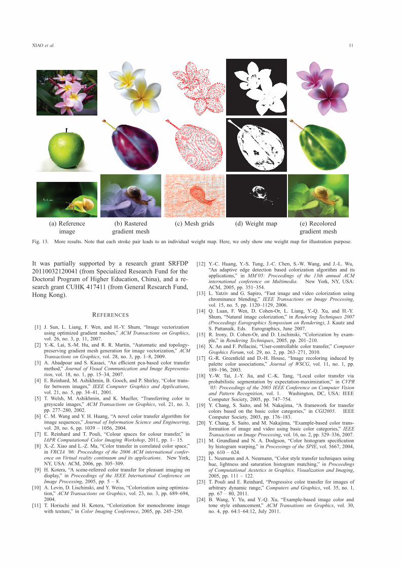
XIAO et al. 11
(a) Reference
image
(b) Rastered
gradient mesh
(c) Mesh grids (d) Weight map (e) Recolored
gradient mesh
Fig. 13. More results. Note that each stroke pair leads to an individual weight map. Here, we only show one weight map for illustration purpose.
It was partially supported by a research grant SRFDP
20110032120041 (from Specialized Research Fund for the
Doctoral Program of Higher Education, China), and a re-
search grant CUHK 417411 (from General Research Fund,
Hong Kong).
REFERENCES
[1] J. Sun, L. Liang, F. Wen, and H.-Y. Shum, “Image vectorizationusing optimized gradient meshes,” ACM Transactions on Graphics,vol. 26, no. 3, p. 11, 2007.
[2] Y.-K. Lai, S.-M. Hu, and R. R. Martin, “Automatic and topology-preserving gradient mesh generation for image vectorization,” ACMTransactions on Graphics, vol. 28, no. 3, pp. 1–8, 2009.
[3] A. Abadpour and S. Kasaei, “An efficient pca-based color transfermethod,” Journal of Visual Communication and Image Representa-tion, vol. 18, no. 1, pp. 15–34, 2007.
[4] E. Reinhard, M. Ashikhmin, B. Gooch, and P. Shirley, “Color trans-fer between images,” IEEE Computer Graphics and Applications,vol. 21, no. 5, pp. 34–41, 2001.
[5] T. Welsh, M. Ashikhmin, and K. Mueller, “Transferring color togreyscale images,” ACM Transactions on Graphics, vol. 21, no. 3,pp. 277–280, 2002.
[6] C. M. Wang and Y. H. Huang, “A novel color transfer algorithm forimage sequences,” Journal of Information Science and Engineering,vol. 20, no. 6, pp. 1039 – 1056, 2004.
[7] E. Reinhard and T. Pouli, “Colour spaces for colour transfer,” inIAPR Computational Color Imaging Workshop, 2011, pp. 1– 15.
[8] X.-Z. Xiao and L.-Z. Ma, “Color transfer in correlated color space,”in VRCIA ’06: Proceedings of the 2006 ACM international confer-ence on Virtual reality continuum and its applications. New York,NY, USA: ACM, 2006, pp. 305–309.
[9] H. Kotera, “A scene-referred color transfer for pleasant imaging ondisplay,” in Proceedings of the IEEE International Conference onImage Processing, 2005, pp. 5 – 8.
[10] A. Levin, D. Lischinski, and Y. Weiss, “Colorization using optimiza-tion,” ACM Transactions on Graphics, vol. 23, no. 3, pp. 689–694,2004.
[11] T. Horiuchi and H. Kotera, “Colorization for monochrome imagewith texture,” in Color Imaging Conference, 2005, pp. 245–250.
[12] Y.-C. Huang, Y.-S. Tung, J.-C. Chen, S.-W. Wang, and J.-L. Wu,“An adaptive edge detection based colorization algorithm and itsapplications,” in MM’05: Proceedings of the 13th annual ACMinternational conference on Multimedia. New York, NY, USA:ACM, 2005, pp. 351–354.
[13] L. Yatziv and G. Sapiro, “Fast image and video colorization usingchrominance blending,” IEEE Transactions on Image Processing,vol. 15, no. 5, pp. 1120–1129, 2006.
[14] Q. Luan, F. Wen, D. Cohen-Or, L. Liang, Y.-Q. Xu, and H.-Y.Shum, “Natural image colorization,” in Rendering Techniques 2007(Proceedings Eurographics Symposium on Rendering), J. Kautz andS. Pattanaik, Eds. Eurographics, June 2007.
[15] R. Irony, D. Cohen-Or, and D. Lischinski, “Colorization by exam-ple,” in Rendering Techniques, 2005, pp. 201–210.
[16] X. An and F. Pellacini, “User-controllable color transfer,” ComputerGraphics Forum, vol. 29, no. 2, pp. 263–271, 2010.
[17] G.-R. Greenfield and D.-H. House, “Image recoloring induced bypalette color associations,” Journal of WSCG, vol. 11, no. 1, pp.189–196, 2003.
[18] Y.-W. Tai, J.-Y. Jia, and C.-K. Tang, “Local color transfer viaprobabilistic segmentation by expectation-maximization,” in CVPR’05: Proceedings of the 2005 IEEE Conference on Computer Visionand Pattern Recognition, vol. 1. Washington, DC, USA: IEEEComputer Society, 2005, pp. 747–754.
[19] Y. Chang, S. Saito, and M. Nakajima, “A framework for transfercolors based on the basic color categories,” in CGI2003. IEEEComputer Society, 2003, pp. 176–183.
[20] Y. Chang, S. Saito, and M. Nakajima, “Example-based color trans-formation of image and video using basic color categories,” IEEETransactions on Image Processing, vol. 16, no. 2, pp. 329–336, 2007.
[21] M. Grundland and N. A. Dodgson, “Color histogram specificationby histogram warping,” in Processings of the SPIE, vol. 5667, 2004,pp. 610 – 624.
[22] L. Neumann and A. Neumann, “Color style transfer techniques usinghue, lightness and saturation histogram matching,” in Proceedingsof Computational Aestetics in Graphics, Visualization and Imaging,2005, pp. 111 – 122.
[23] T. Pouli and E. Reinhard, “Progressive color transfer for images ofarbitrary dynamic range,” Computers and Graphics, vol. 35, no. 1,pp. 67 – 80, 2011.
[24] B. Wang, Y. Yu, and Y.-Q. Xu, “Example-based image color andtone style enhancement,” ACM Transations on Graphics, vol. 30,no. 4, pp. 64:1–64:12, July 2011.
12 ACCEPTED BY IEEE TRANSACTIONS ON MULTIMEDIA
[25] Y. Ji, H.-B. Liu, X.-K. Wang, and Y.-Y. Tang, “Color transfer togreyscale images using texture spectrum,” in Proceedings of theThird International Conference on Machine Learning and Cyber-netics, 2004, pp. 4057 – 4061.
[26] G. Charpiat, M. Hofmann, and B. Scholkopf, “Automatic imagecolorization via multimodal predictions,” in Proceedings of the 10thEuropean Coference on Computer Vision, vol. 3, 2008, pp. 126 –139.
[27] J. Li and P. Hao, “Transferring colours to grayscale images by locallylinear embedding,” in Proceedings of the British Machine VisionConference, 2008, pp. 835 – 844.
[28] Y. Morimoto, Y. Taguchi, and T. Naemura, “Automatic colorizationof grayscale images using multiple images on the web,” in Proceed-ings of Siggraph Posters, 2009, p. 32.
[29] X.-Z. Xiao and L.-Z. Ma, “Gradient-preserving color transfer,”Computer Graphics Forum, vol. 28, no. 7, pp. 1879–1886, 2009.
[30] F. Pitie, A. C. Kokaram, and R. Dahyot, “Automated colour gradingusing colour distribution transfer,” Computer Vision and ImageUnderstanding, vol. 107, no. 1-2, pp. 123–137, 2007.
[31] Q. Luan, F. Wen, and Y.-Q. Xu, “Color transfer brush,” in PG ’07:Proceedings of the 15th Pacific Conference on Computer Graphicsand Applications. Washington, DC, USA: IEEE Computer Society,2007, pp. 465–468.
[32] C.-L. Wen, C.-H. Hsieh, B.-Y. Chen, and M. Ouhyoung, “Example-based multiple local color transfer by strokes,” Computer GraphicsForum, vol. 27, no. 7, pp. 1765–1772, 2008.
[33] J. Ferguson, “Multivariable curve interpolation,” J. ACM, vol. 11,no. 2, pp. 221–228, 1964.
[34] P. F. Felzenszwalb and D. P. Huttenlocher, “Efficient graph-basedimage segmentation,” International Journal of Computer Vision,vol. 59, p. 2004, 2004.
[35] C. Rother, V. Kolmogorov, and A. Blake, “Grabcut: Interactiveforeground extraction using iterated graph cuts,” ACM Transactionson Graphics, vol. 23, pp. 309–314, 2004.
[36] Y. Xiang, B. Zou, and H. Li, “Selective color transfer with multi-source images,” Pattern Recognition Letters, vol. 30, no. 7, pp. 682– 689, 2009.
[37] D. Hasler and S. Susstrunk, “Measuring colorfulness in naturalimages,” in Proc. IS&T/SPIE Electronic Imaging 2003: HumanVision and Electronic Imaging VIII, vol. 5007, 2003, pp. 87–95.
[38] Y. C. X. S. Chen, Guanhao, “Gradient-based structural similarityfor image quality assessment,” in Proc. of 2006 IEEE InternationalConference on Image Processing, 2006, pp. 2929–2932.
[39] G. Wolberg and I. Alfy, “Monotonic cubic spline interpolation,” inProc. of Computer Graphics International, 1999, pp. 188–195.
Yi Xiao received the Bachelor’s degree and Mas-ter’s degree in Mathematics from Sichuan Uni-versity in 2005 and 2008, and the PhD. degree inElectronic Engineering from City University ofHong Kong in 2012. He is currently a Senior Re-search Associate in the Department of ElectronicEngineering, City University of Hong Kong. Hisresearch interests include Neural Networks andComputer graphics.
Liang Wan received the B.Eng and M.Engdegrees in computer science and engineer-ing from Northwestern Polytechnical University,P.R. China, in 2000 and 2003, respectively. Sheobtained a Ph.D. degree in computer scienceand engineering from The Chinese Universityof Hong Kong in 2007. She is currently anAssociate Professor in the School of Com-puter Software, Tianjin University, P. R. China.Her research interest is mainly on computergraphics, including image-based rendering, non-
photorealistic rendering, pre-computed lighting, and image processing.
Chi-Sing Leung received the B.Sci. degree inelectronics, the M.Phil. degree in informationengineering, and the PhD. degree in computerscience from the Chinese University of HongKong in 1989, 1991, and 1995, respectively. Heis currently an Associate Professor in the Depart-ment of Electronic Engineering, City Universityof Hong Kong. His research interests includeneural computing, data mining, and computergraphics. In 2005, he received the 2005 IEEETransactions on Multimedia Prize Paper Award
for his paper titled, “the Plenoptic Illumination Function” published in2002. He is the Program Chair of ICONIP2009. He is also a governingboard member of the Asian Pacific Neural Network Assembly (APNNA).
Yu-Kun Lai received his bachelor’s degree andPhD degree in computer science from TsinghuaUniversity in 2003 and 2008, respectively. Heis currently a lecturer of visual computing inthe School of Computer Science and Informatics,Cardiff University, Wales, UK. His research in-terests include computer graphics, geometry pro-cessing, image processing and computer vision.
Tien-Tsin Wong received the B.Sci., M.Phil.,and Ph.D. degrees in computer science from theChinese University of Hong Kong in 1992, 1994,and 1998, respectively. Currently, he is a Profes-sor in the Department of Computer Science &Engineering, The Chinese University of HongKong. His main research interest is computergraphics, including perception graphics, com-putational manga, image-based rendering, GPUtechniques, natural phenomena modeling, andmultimedia data compression. He received IEEE
Transactions on Multimedia Prize Paper Award 2005, Young ResearcherAward 2004. He is also the awardee of National Thousand Talents Planof China 2011.