This document is downloaded from the Digital Open Access Repository of VTT

VTT http://www.vtt.fi P.O. box 1000 FI-02044 VTT Finland

By using VTT Digital Open Access Repository you are bound by the following Terms & Conditions.

I have read and I understand the following statement:

This document is protected by copyright and other intellectual property rights, and duplication or sale of all or part of any of this document is not permitted, except duplication for research use or educational purposes in electronic or print form. You must obtain permission for any other use. Electronic or print copies may not be offered for sale.

Title On the use of fractional Brownian motion in the theory of connectionless networks

Author(s) Norros, Ilkka Citation IEEE Journal on Selected Areas in

Communications vol. 13(1995):6, pp. 953-962

Date 1995 URL http://dx.doi.org/10.1109/49.400651 Rights Copyright © (1995) IEEE.

Reprinted from IEEE Journal on Selected Areas in Communications. This article may be downloaded for personal use only

IEEE JOURNAL ON SELECTED AREAS IN COMMUNICATIONS, VOL. 13, NO. 6, AUGUST 1995 953

On the Use of Fractional Brownian Motion in the Theory of Connectionless Networks

Ilkka Nomos

Abstrucl- An abstract model for aggregated connectionless traffic, based on the fractional Brownian motion, is presented. Insight into the parameters is obtained by relating the model to an equivalent burst model. Results on a corresponding storage process are presented. The buffer occupancy distribution is ap- proximated by a Weibull distribution. The model is compared with publicly available samples of real Ethernet traffic. The degree of the short-term predictability of the traffic model is studied through an exact formula for the conditional variance of a future value given the past. The applicability and interpretation of the self-similar model are discussed extensively, and the notion of ideal free traffic is introduced.

I. INTRODUCTION N this paper we consider the modeling of traffic phenom- I ena in a connectionless network. The principle of such a

network is that all data is sent in relatively small indepen- dent pieces, packed in so called datagrams labeled with the destination address. No bandwidth needs to be reserved. The emerging available bit rate service in asynchronous transfer mode (ATM) networks has the latter feature also, even though ATM is a connection oriented service, and thus a lot of this paper is applicable to this service as well.

The connectionless transfer makes efficient sharing of re- sources possible in the case that the traffic sources are bursty, i.e., they are not transmitting continuously but have silent or low-activity periods alternating with periods of high activity. This is typical for computer communications. Moreover, the traffic is usually bursty at several timescales. For example, the activity of a person’s workstation depends on the general character of hisher present work and on the particular task, and it consists of several kinds of sessions, which again can contain many short traffic-intensive operations like file transfers.

A condition for the success of connectionless communica- tion is some flexibility of the partners. The performance of the network depends on the unpredictable activity of the other users, and it must be accepted that, for example, file transfer is sometimes slower than normal. There is considerable interest in using the existing connectionless networks and their more effective future counterparts for real-time services like voice and video, and the speed requirements for data traffic are becoming more stringent as well, so the problem of appropriate modeling of connectionless traffic has practical importance.

Modeling is based on understanding what is essential. In our context, one can in fact distinguish between two types of understanding: concrete causal understanding and abstract

Manuscript received September 30, 1994; revised April 1 , 1995. The author is with VTT Telecommunications, 02044 VTT Finland. IEEE Log Number 9412645.

statistical understanding. In the former, one thinks of events like file transfers and sessions and builds the total traffic model by combining element models. In the latter, one finds a stochastic model for the total traffic which is mathematically nice and has some of the essential statistical properties but does not contain models for more elementary events and remains in this sense abstract.

In the case of connectionless traffic, concrete modeling is practically impossible because the traffic consists of so many different elements. Therefore it was a truly great dis- covery when W. Leland’s group in Bellcore found that the multi-timescale burstiness of local area network (LAN) traffic could be well characterized with a very simple notion-self- similarity. In late spring 1992, working within the project RACE 2032 COMBINE, I studied the paper by Fowler and Leland [7] and proposed a three-parameter Gaussian traffic model with self-similar variation. Later I learned that within Leland’s group self-similar models were not only identified as promising but their applicability had been extensively studied with surprisingly positive results. This work has obtained wide publicity, in particular after its presentation in Proc. ACM SIGCOMM I993 [ 151.

The aim of the present paper is to summarize and discuss certain properties of the above mentioned Gaussian model. The three main themes are understanding the parameters of the model, the properties of a queue with self-similar input, and short-term traffic prediction. The paper is organized as follows. The model is introduced and its parameters discussed in Section 11. The properties of a storage with self-similar input are considered in Section 111. Short-term traffic prediction is the theme of Section IV. The problems of the applicability of the model, in particular its relation to the transport layer protocol, are discussed in Section V. Finally, some conclusions are summarized in Section VI.

11. A GAUSSIAN SELF-SIMILAR TRAFFIC MODEL

A. Preliminaries

Let us consider an element of a connectionless network (e.g., an Ethernet section) and denote by At the amount of traffic (in bits, say) offered to it in the time interval [0 , t ) . In particular, we always have A0 = 0. Let At be defined for all t E (-ea, m) and denote the traffic offered in [s . t ) by A(s , t ) = A , - A,. A true cumulating arrival process is of course an increasing process. We shall, however, not emphasize this since below we shall model the traffic with a Gaussian process A, which necessarily has negative increments also.

0733-8716/95$04.00 0 1995 IEEE

954

-0.6;

IEEE JOURNAL ON SELECTED AREAS IN COMMUNICATIONS, VOL. 13, NO. 6, AUGUST 1995

We always assume that the process At has stationary increments, i.e., that for any t E % and s1 < . . . < s, the distribution of

(A(t + SI. t + SZ), . . . , A( t + ~ ~ - 1 , t + s n ) )

is independent of t . We also assume square integrability, i.e., EA: < CO. It follows from the stationarity of the increments that EAt = mt for some constant m, the mean rate, and that, denoting v(t) = VarA+

1 2

CovA,,At = - ( v ( t ) + t f ( ~ ) - v ( t - s ) )

for s < t . Thus, the correlation structure (all so called second- order properties) of At is determined by the variance function v(t) alone.

The process At is called short-range dependent if for any s < t 5 U < v the correlation coefficient between A(as,at) and A ( a u , a v ) converges to zero when the time scale a approaches infinity. Otherwise it is called long- range dependent. If At is short-range dependent, v ( t ) is asymptotically linear. In particular, if At is a process with independent increments, say a Poisson process or a compound Poisson process, then w ( t ) is a linear function.

All traffic models traditionally used in teletraffic theory are short-range dependent. From this point of view it was rather shocking that the accurate and extensive LAN traffic measurements conducted in Bellcore [ 151 gave variance curves where v ( t ) grew rather accurately as a fractional power t p ,

with p taking values strictly between 1 and 2, through half a dozen of orders of magnitude. It became obvious that at least some traffic phenomena had to be studied with long-range dependent models.

The power form v ( t ) = tP is closely related to the fascinat- ing fractal nature of the traffic traces recorded at Bellcore. Indeed, the time-scaled process A,t then has the variance function

V,arAmt = (at)P = aPVarAt

which implies that Aat and apI2At have the same correlation structure, i.e., the centered process At - mt is second-order self-similar. Note that a second-order self-similar process is long-range dependent unless it has uncorrelated increments, and that the (centered) Poisson process is second-order self- similar (with p = 1).

A process Yt is called (strictly) selfsimilar with Hurst parameter (or self-similarity parameter) H if, for any a > 0, the processes Yet and aH& have the same finite-dimensional distributions. Obviously, self-similarity and second-order self- similarity are equivalent for Gaussian processes since their finite dimensional distributions are by definition Gaussian and thus fully characterized by their first and second-order moments. By an important theorem of Lamperti [14], self- similarity is a generic property of wide classes of limit processes. As a general reference to self-similar processes, see, e.g., articles in the collection [5] .

When a model is built on second-order properties alone, a Gaussian process is often the simplest choice. In this paper we shall model the variation of connectionless traffic with a

0 . 2 0 . 4 0 . 6 0 .8 1.0 -0.1

v Fig. 1. A realization of Zt , t E [0,1] with H = 0.8

Gaussian self-similar process, a fractional Brownian motion (FBM). A normalized FBM with Hurst parameter H E [i, 1) is a stochastic process Zt, t E (-m, CO) , characterized by the following properties:

1) 2, has stationary increments; 2) 2, = 0, and EZt = 0 for all t ; 3) EZ? = Jt12H for all t ; 4) Zt has continuous paths; and 5 ) 2, is Gaussian, i.e., all its finite-dimensional marginal

distributions are Gaussian. This process was found by Kolmogorov [12], but relatively little attention was paid to it before the pioneering paper by Mandelbrot and Van Ness [16] (where the FBM also got its present name). In the special case H = l / 2 , Zt is the standard Brownian motion. We have ruled out the other limiting case H = 1 since the respective 2, is a deterministic process with linear paths.

The covariance of the increments in two nonoverlapping intervals is always positive and has the expression

covzt, - zt, , zt, - zt, 1 2

= - ((t4 - t p - (t3 - t p

+(t3 - t 2 y - (t4 - t p )

for tl < t2 5 t 3 < t4. Many features of FBM’s with H > 1/2 are different

from those of most stochastic processes usually appearing in traffic models. They are not Markov processes and not even semimartingales, having nondifferentiable paths with zero quadratic variation. Fig. 1 presents a simulated realization of Zt with H = 0.8, produced with a simple but somewhat inaccurate bisection method given in [17]. Note that the path looks considerably smoother than that of an ordinary Brownian motion.

For the use of the FBM as a traffic model element it is pleasant to note that in spite of the strong correlations, it is ergodic in the sense that the stationary sequence of increments Zn+l - 2, is ergodic (e.g., [2], Theorem 14.2.1).

B. Fractional Brownian TrafJic

model defined as follows. The rest of this paper is devoted to the -study of a traffic

NORROS: ON THE USE OF FRACTIONAL BROWNIAN MOTION 955

Definition 2.1: We call the process

At = mt + G Z , , t E (-x, cm) (2)

where Zt a normalized FBM, fractional Brownian trafic. The process has three parameters m, a and H with the following interpretations: m > 0 is the mean input rate, a > 0 is a variance coefficient, and H E [1/2,1) is the Hurst parameter of 2,. In the special case H = 1/2 we call At Brownian trafic.

Remark 2.2: Z ( t ) is a mathematical object which has no physical dimension and its parameter t is dimensionless as well. Therefore it would be better to write it in the traffic model as Z(t/ t ,) , where t is physical time and tu is the physical time unit. This helps, in particular, to avoid confusion by a change of the time unit. However, we shall not do this in order to keep our notation simple. If work is measured in bits and time in seconds, a has the dimension bit . s. The Hurst parameter H is dimensionless.

The factor fi in (2) is motivated by the following easily verified superposition property: The sum At = A!a) of K independent fractional Brownian traffics with common parameters a and H but individual mean rates mi can be written as At = mt + JmaZt , where m = ma and Zt is a FBM with parameter H . This shows that the roles of the three parameters of the traffic model (1) can be separated so that H and a characterize the “quality” of the traffic in contrast to the long run mean rate m which characterizes its “quantity” alone.

C. Parameter Interpretation with a Burst Model

More insight into the roles of the three parameters can be obtained by relating fractional Brownian traffic to another simple long-range dependent traffic model, namely a fluid burst model where the burst length has infinite variance. Assume that the arriving traffic consists of (“fluid”) bursts that begin according to a Poisson process with parameter A, come with rate T each and have independent total volumes B, with joint distribution F ( z ) = P(B 5 x). The length of burst n in time is then T, = BTL/r , and P(T 5 t ) = F(7-t). This kind of fluid flow models have been widely used in teletraffic theory since Kosten’s seminal paper [13], but the corresponding storage system cannot be analyzed in our case with the Markovian tools usually applied in this context.

Denote the number of bursts going on at time t by Kt. It is then standard knowledge (the system can be considered as an M/G/cm system) that the system can be made stationary if and only if the mean burst size b = EB is finite. Then EK = XET and

COvKt, Kt+h X (1 - F(rs))ds. r Note that any correlation function p(h) such that p(h) \ 0 and p ’ ( h ) \ 0 for h /” cm can be realized by this type of rate process. The system is long-range dependent if

COVKO, Ktdt = ET2 = x I* (this is equivalent to our previous definition, see [3]), i.e., exactly when B has infinite variance.

Denote the fluid arrival rate at time t by Rt = rKt . The mean arrival rate is then m = ER = Ab. A straightforward calculation gives two useful expressions for the variance of the cumulating arrival process At = Ji R,ds

r t r t

= 2Xrb 1 du Jo’ dv P ( U > T U )

: IU

(3)

= A~b(2tE((U/7) A t ) - E ( ( U / r ) A t)’) (4)

where U is a random variable that has the “residual lifetime” distribution corresponding to that of B in the renewal theory sense, i.e.,

P ( U 5 U ) = - (1 - F ( t ) ) d t .

Note that if B has infinite variance, then U has an infinite expectation.

Assume now that the distribution F ( z ) has tail behavior of type xd with /3 E (-2, -1) in the sense that for any t > 0 there exist positive constants y and r such that

yd-t 5 1 - F ( ~ ) 5 r z P + € .

It then follows from (3) that VarAt grows asymptotically (in the above sense) as VarAt N Since p + 3 E (1,2), this is of the same type as by fractional Brownian traffic with H = (0 + 3)/2. Note that H does not depend on the other parameters of the fluid model. This suggests an intuitive understanding of high Hurst parameter values as coming from the distribution of very long bursts (or activity periods, etc.). It has been indeed often observed that activity periods of a traffic source have “heavy-tailed” distributions (see, e.g., [23]).

This connection between long-range dependence, activity periods with infinite variance and self-similarity was estab- lished by Mandelbrot who considered the convergence of aggregations of so called renewal reward processes with heavy-tailed inter-renewal distributions toward an FBM. For exact convergence results on renewal reward processes (which are, however, not quite the same thing as our present fluid model), see [22]. The asymptotic self-similarity of the fluid model considered here was noted, in terms of the M/G/oo system, in [3], and referred to in [15]. A detailed traffic model of this type has been proposed at least in [24].

It remains to study what corresponds to the variance param- eter a of fractional Brownian traffic in an “equivalent” fluid burst model. Equating the variances of At for large t in both models we get the equation

VarAt = 7natZH = X ~ b ( 2 t E ( ( U / r ) A t ) - E ( ( U / T ) A t ) 2 ) .

Substituting m = Ab, dividing by t 2 H , choosing t sufficiently large to make the right hand side approximately independent of it, and denoting then x0 = r t , we finally get

a = r,2H-1.ro2H(2.roE(U A L O ) - E(U A TO)’) (5)

where zo can be considered as a boundary (rather arbitrary upwards) between “small” and “large” bursts. Thus, we can

956 IEEE JOURNAL ON SELECTED AREAS IN COMMUNICATIONS, VOL. 13, NO. 6, AUGUST 1995

TABLE I ESTIMATES FOR m , CL, AND H FROM THE BELLCORE SAMPLE pOct.TL, FROM A SIMULATED REALIZATION OF FRACTIONAL BROWNIAN TRAFFIC WITH PARAMETERS

TAKEN FROM THE pOct.TL COLUMN AND FROM THE SAMPLE 0ctExt.TL

6Mb/s

0 2 0 0 400 600 8 0 0 1000 [sec] (b)

Fig. 2. The variation of the bitrate (b/s, averaged over intervals of 1 s) in the true Ethernet trace pOct.TL (upper graph) and a simulated realization of fractional Brownian traffic with the same parameters (lower graph).

make the following observations on the parameter a in terms of an equivalent fluid burst model:

a is independent of A; when H = l / 2 , a is the index of dispersion (variance over mean) of A, for large t , and it is independent of the burst transmission rate T . Note that H = 1 /2 means that “all bursts are short,” and at a large time scale their arrivals can be considered instantaneous; when H > l / 2 , a is the product of three factors; the first factor rZH-l gives an interesting expression for a’s dependence on the burst transmission rate T ; the first two factors together show that a depends on H through a factor of the form constZH. The remaining factor depends mainly on the truncated distribution of B for “short bursts .”

D. An Experiment with Bellcore Data

Let us compare the FBM traffic model with a trace of actual Bellcore Ethernet traffic data from October 1989 (avail- able with anonymous FTP from jlash.bellcore.com, directory pub/lun_trufJic, file pOct.TL). It contains the time stamps and lengths of 1 000 000 consecutive packets. For convenience, we

200kb/s

150kb/s

lOOkb/s

50kb/s I

Fig. 3. sample of seven daytime hours of external traffic in Bellcore.

The variation of the bitrate (b/s, averaged over intervals of 8 s) in a

restrict to the first 1024 s of the trace (the whole trace it not much longer).

The parameters a and H were estimated by linear regression from the logarithms of the sample variances for 2k s, k = -5: . . . ,4 . A simulated sample of the FBM model was created with the same parameter set (using, in fact, the same method and pseudorandom sequence as in Fig. 1). For a check, the parameters were also estimated from the simulated sample. Both parameter sets are given in Table I. The accuracy of the algorithm is satisfactory for our present purposes. Fig. 2 shows the profiles of both traces. The visual similarity is considerable.

Let us then consider another Bellcore trace (file 0ctExt.TL in the same directory), where only the external traffic between Bellcore and the rest of the world is recorded. This formed only a small portion of the total traffic. The second-order self- similarity was quite strong in both samples in the sense that the above mentioned logarithms of sample variances formed straight lines. Fig. 3 shows the variation of the transmission rate during 7 daytime hours, averaged over intervals of 8 s, and the estimated parameters rn, a and H are given in the rightmost column of Table I. The most obvious difference from the previous sample is that the overall mean rate m is much lower than the mean deviations of averages over intervals even in the order of magnitude of seconds. The distribution of the local rate is thus strongly non-Gaussian, which indicates that the traffic is not aggregated from sufficiently many independent streams to allow the applicability of a Gaussian model. The corresponding fractional Brownian traffic looks essentially similar to that of Fig. 2 and thus has almost half of the total arrivals in the averaging intervals negative.

It is interesting that the parameter a is so much lower and H clearly higher in the latter case. Tentative explana- tions suggested by the findings of Section 11-C could be the lower transmission rates of long-distance data traffic and the dominance of file transfer, respectively.

111. THE QUEUE WITH GAUSSIAN SELF-SIMILAR INPUT

A. Definition of the Storage Process

Let us now turn to the problem of buffering of traffic fluctuations. Assume that fractional Brownian traffic with certain parameters m, a, and H is offered to a link with capacity C > rn that has an unlimited buffer in front of it. The buffer occupancy can be defined in analogy to Reich’s formula

NORROS: ON THE USE OF FRACTIONAL BROWNIAN MOTION 957

In the Brownian case H = 1/2, (8) reduces to

l-p . x = const (9)

with p = 7n/C. Here we may roughly say that reducing the relative free capacity 1 - p by half costs doubling the storage size. Note that the link capacity C does not appear in the equation except within p.

With H > l / Z the situation is different. Let us first write

Pa

(8) in the form of a buffer dimensioning formula - VPC p m - H ) )

(1 - o)H/(l--H) = f - 1 ( t )a1 / (2 (1-H) )C(2H--1) l (2 (1~H))

Fig. 4. connections.

Reduction of VPC's by the use of a CLS instead of pairwise ATM

for the virtual waiting time in a queueing system ([20], cited according to [l]).

Dejinition 3. I : The (stationary) fractional Brownian stor- age with input parameters m, a and H and output capacity C > m is the stochastic process X t defined as

X t SUP (At - A , - C( t - s ) ) , t E (-CO, CO) (6) s s t

where At is the fractional Brownian traffic process with parameters m, n and H . In the special case H = l / Z we call X t the Brownian storage.

The stationarity of X t follows from the stationarity of the increments of A t . That X t is almost surely finite is a consequence of Birkhoff's ergodic theorem. Indeed, the ergodicity of Zt implies that limt,, Zt / t = E21 = 0 a.s., which together with the assumption rn < C yields

lim ( A t - A , - C( t - s ) ) = --x as. Y ' - m

Note that the storage process X t is always nonnegative, although the arrival process has also negative increments.

B. A Scaling Law

The fractional Brownian storage X t obeys an interesting scaling law which is easily deduced from the self-similarity of the FBM. Consider the typical requirement that the probability that the amount of work in system exceeds a certain level x must be small. (The value x is the substitute for the buffer size in our infinite storage model.) If the largest allowed buffer saturation probability (or time congestion probability) is t, then the equation

t = P(X > x) (7)

holds at the maximal allowed load. Now, the self-similarity of Zt allows for deriving from (7) a more explicit relation between the design parameters x (buffer space, or requirement) and C (link capacity) and the traffic parameters m, a and H at the critical boundary.

Theorem 3.2: [ 181 Assuming (7), the following equation holds

where the function

\ V I

(10) It is seen that when H is high, a substantial increase in utiliza- tion, say again halving the free capacity, requires a tremendous amount more storage space. Thus we have a new argument for the widely accepted view that for connectionless packet traffic the utilization factor cannot be practically improved by enlarging the buffers.

The scaling relation (8) can also be written as the bandwidth allocation rule

C = + ~ ~ l ( ~ ) a l / ( 2 H ) x - ( l - H ) / H ~ ~ ~ l / ( z H ) (11)

showing that, for H > l / Z , the link requirement C increases slower than linearly in m so that a multiplexing gain is obtained by using links with higher capacity.

As a practical example where the multiplexing gain plays a central role, compare the use of painvise ATM virtual path connections (VPC's) between n + 1 LAN/ATM intenvorking units (IWU's) with the use of a centralized routing function (connectionless server (CLS)). The essential difference be- tween an ATM switch and a CLS is that the former performs switching purely at the ATM layer whereas the latter looks at the network layer address, found in the payload of the first cell of each datagram. The two alternatives, called in [lo] indirect and direct connectionless service provision over an ATM network, respectively, are depicted in Fig. 4 in the case ri = 3.

Denote the bandwidth needed per IWU with centralized routing by Cdir and the total bandwidth needed per IWU with painvise VPC's by Cindir,n. Assume that a fixed amount x of output buffer space is allocated for any VPC and that all traffic streams between the IWU's are equal. It is then seen from (1 1) that

Cin&r,lL = m + (Cdir - m)711-1 ' (2H) . (12)

Note that this expression for the relative multiplexing gain does not contain the unknown factor f - ' ( t ) .

C. The Approximate Queue Length Distribution

No explicit formula for the distribution of the fractional Brownian storage seems to be known. Instead, we shall approach the distribution of X t through a lower bound.

Theorem 3.3: [ 181 Let X t be the fractional Brownian stor- age with parameters m, a , H and C. Then

depends on H but not on m, a , C or x.

958 IEEE JOURNAL ON SELECTED AREAS IN COMMUNICATIONS, VOL. 13, NO. 6, AUGUST 1995

-1 -2

-3

-4

- 5

- 6

-7

x .t

Fig. 5. Weibull approximation of log,, P(X > .r) with 711 and a as in the Bellcore sample pOct.TL, C = 4.8 Mb/s and H = 0.5, 0.6. 0.7. 0.8, and 0.9.

where r;(H) = ”(1 - H ) l - H and q(y) = P(Z1 > y) is the residual distribution function of the standard Gaussian distribution.

This result is a consequence of the trivial lower bound

P ( X > x) 2 maxP(At > Ct + x) (14)

where the maximum at the right hand side is obtained at t = N z / ( ( l - H ) ( C - m)). It has been recently shown by Duffield and O’Connell [4] with techniques of the theory of large deviations that (16) below is in fact logarithmically accurate for large x. This is in line with the intuitive principle that “rare events occur only in the most probable way.”

t>o

Using further the approximation - W Y ) exP(-Y2/2) (15)

we obtain the expression

Thus, the distribution of Xt can be approximated by a Weibull distribution, in particular as regards the tail behavior.

Remark 3.4: In line with Remark 2.2, the right-hand side of (1 6) can be written in the form

where tu is the physical time unit, making the probability expression explicitly dimensionless.

Fig. 5 shows the residual distribution function of the Weibull distribution (16) with different values of H , m and a being taken from the first column of Table I and C chosen to be 4.8 Mb/s. (Remember, however, that the consideration of Section 11-C indicates that in a practical situation it might not be fully reasonable to consider the effect of changes in H without respective changes in a.)

It is interesting to look at Fig. 5 from the point of view of the distinction between cell and burst scale traffic fluctuations, often emphasized in the analysis of ATM multiplexers with variable bitrate traffic (e.g., [19]). The sharp knee between the cell and burst scale components of the queue length distribution, observed in studies like the one just mentioned, is here replaced by continuous flattening, corresponding to the

7Mbls

5Mb/ s

3Mb/s

I !

/

0 200 400 [kbitsec] Fig. 6. Required link capacity as a function of a with m = 2 Mb/s and H = 0.5, 0.7, and 0.9. The upper three curves (as at the right) correspond to the buffer size 100 kbytes and the lower three to the buffer size 1 Mbyte.

intuitive idea of “burstiness in all time scales.” In particu- lar, the curves don’t have nonzero asymptotic slopes when H > l / 2 .

In the Brownian case H = l /2 , the Weibull distribution (16) reduces to the exponential distribution

It is interesting to note that the lower bound approximation (14) and approximation (15) happen to cancel out each other so that the right-hand side of (17) gives in fact exactly P(X > x) for the Brownian storage [21, ch. 61.

Solving (16) for C we see that P(X > x) = E is achieved approximately when

C = + ( ~ ( ~ j ~ ~ ) ~ ~ ~ a ’ / ~ 2 ” ~ ~ - ~ l - ” ~ / H m l / ~ 2 H ~ .

(18) Note that by the exact scaling relation (1 l), the only approx- imate part of (18) is the coefficient in front of the powers of a, x and m.

For practical use of (18) as a link dimensioning formula, it is interesting to consider its sensitivity on a and H . Fig. 6 depicts the link recommendation with various values of a and H for m = 2 Mb/s, E = lop3 and for the two buffer sizes 100 kbytes and 1 Mbyte. Of course, the same reservation as with the previous figure should be made on the meaningfullness of independent variation of a and H . In any case, it is seen that when the buffer is small, the link requirement depends much less on H than when the buffer is large. It is very difficult for short-range dependent traffic to fill a large buffer!

D. A Further Remark on Weibullian Queue Lengths

The Weibull distribution P ( X > x) = e-y lC2-2H with H > 1/2 is a somewhat “unfriendly” distribution which has finite moments but not a finite moment-generating function (Laplace transform) in any neighborhood of zero. Thus it can be expected that long-range dependent queueing systems sometimes have qualitatively different behavior than corresponding short-range dependent systems. An example of such a difference is provided by the following simplistic consideration of a problem of the type “who causes a typical congestion?’

Assume that connectionless traffic from a large number of sources comes to a multiport router from which it is

NORROS: ON THE USE OF FRACTIONAL BROWNIAN MOTION 959

100 200 3 0 0 4 0 0 5 0 0 600 700 [kbit] 0

- 4 .

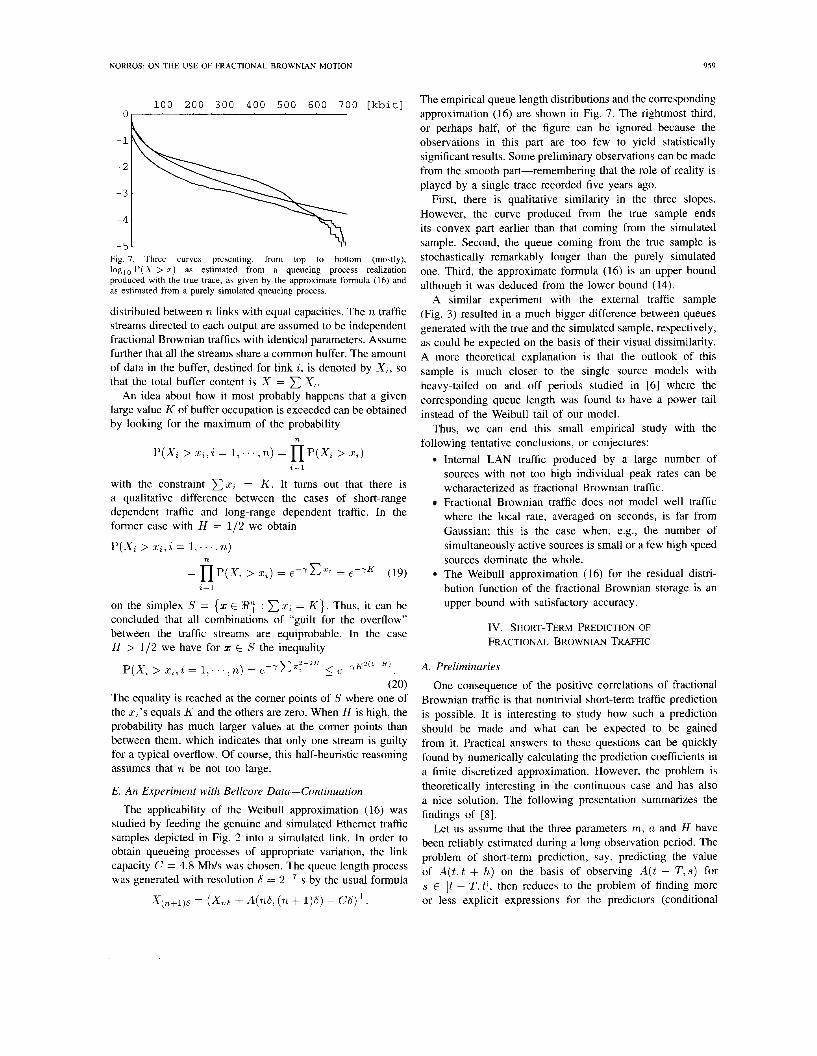
- 5 - Fig. 7. Three curves presenting, from top to bottom (mostly), loglo P(X > .r) as estimated from a queueing process realization produced with the true trace, as given by the approximate formula (16) and as estimated from a purely simulated queueing process.

distributed between n links with equal capacities. The n traffic streams directed to each output are assumed to be independent fractional Brownian traffics with identical parameters. Assume further that all the streams share a common buffer. The amount of data in the buffer, destined for link i , is denoted by X i , so that the total buffer content is X = CXi.

An idea about how it most probably happens that a given large value K of buffer occupation is exceeded can be obtained by looking for the maximum of the probability

n

P(X2 > X 2 , i = 1,. . . , n ) = n P ( X 2 > Xi) i = l

with the constraint Cxi = K . It turns out that there is a qualitative difference between the cases of short-range dependent traffic and long-range dependent traffic. In the former case with H = l / Z we obtain

P(X, > X i r i = 1, ‘ . ’ , n) n

on the simplex S = {z E 87 : 2, = K } . Thus, it can be concluded that all combinations of “guilt for the overflow” between the traffic streams are equiprobable. In the case H > l / Z we have for z E S the inequality

z 2 - 2 H P(X, > x,,i = 1,. . . . n ) = e - c 1

5 e - y K L ( l - H ) .

(20) The equality is reached at the comer points of S where one of the z,’s equals K and the others are zero. When H is high, the probability has much larger values at the corner points than between them, which indicates that only one stream is guilty for a typical overflow. Of course, this half-heuristic reasoning assumes that n be not too large.

E. An Experiment with Bellcore Data-Continuation

The applicability of the Weibull approximation (16) was studied by feeding the genuine and simulated Ethernet traffic samples depicted in Fig. 2 into a simulated link. In order to obtain queueing processes of appropriate variation, the link capacity C = 4.8 Mbls was chosen. The queue length process was generated with resolution b = Z-7 s by the usual formula

X(n+1)6 = ( L 6 + 4 7 1 6 ( n + 1 ) b ) - Cb)+

The empirical queue length distributions and the corresponding approximation (16) are shown in Fig. 7. The rightmost third, or perhaps half, of the figure can be ignored because the observations in this part are too few to yield statistically significant results. Some preliminary observations can be made from the smooth part-remembering that the role of reality is played by a single trace recorded five years ago.

First, there is qualitative similarity in the three slopes. However, the curve produced from the true sample ends its convex part earlier than that coming from the simulated sample. Second, the queue coming from the true sample is stochastically remarkably longer than the purely simulated one. Third, the approximate formula (16) is an upper bound although it was deduced from the lower bound (14).

A similar experiment with the external traffic sample (Fig. 3) resulted in a much bigger difference between queues generated with the true and the simulated sample, respectively, as could be expected on the basis of their visual dissimilarity. A more theoretical explanation is that the outlook of this sample is much closer to the single source models with heavy-tailed on and off periods studied in [6] where the corresponding queue length was found to have a power tail instead of the Weibull tail of our model.

Thus, we can end this small empirical study with the following tentative conclusions, or conjectures:

Internal LAN traffic produced by a large number of sources with not too high individual peak rates can be wcharacterized as fractional Brownian traffic. Fractional Brownian traffic does not model well traffic where the local rate, averaged on seconds, is far from Gaussian; this is the case when, e.g., the number of simultaneously active sources is small or a few high speed sources dominate the whole. The Weibull approximation (16) for the residual distri- bution function of the fractional Brownian storage is an upper bound with satisfactory accuracy.

Iv . SHORT-TERM PREDICTION OF FRACTIONAL BROWNIAN TRAFFIC

A. Preliminaries

One consequence of the positive correlations of fractional Brownian traffic is that nontrivial short-term traffic prediction is possible. It is interesting to study how such a prediction should be made and what can be expected to be gained from it. Practical answers to these questions can be quickly found by numerically calculating the prediction coefficients in a finite discretized approximation. However, the problem is theoretically interesting in the continuous case and has also a nice solution. The following presentation summarizes the findings of [SI.

Let us assume that the three parameters m, a and H have been reliably estimated during a long observation period. The problem of short-term prediction, say, predicting the value of A(t , t + h) on the basis of observing A( t - T, s ) for s E [t - T , t ] , then reduces to the problem of finding more or less explicit expressions for the predictors (conditional

960 IEEE JOURNAL ON SELECTED AREAS IN COMMUNICATIONS, VOL. 13, NO. 6, AUGUST 1995

0 . 6 -

0 . 4

0 . 2

I -1 - 0 . 5 0

The prediction weight function gl(1, t ) for H = 0.9. The function Fig. 8. approaches infinity at both ends of the interval.

~

-

expectations)

Z h , T = E[Zh I z s , S E (-T,0]], h > 0,T E (0, W].

It would be natural to represent the predictors as integrals over the observed part of the process in the form

0

Zh,T = lT gT(hr t)dzt (21)

where gT(h, t) is an appropriate weight function. When the integrand is a smooth deterministic function, an integral w.r.t. 2, can be defined simply as a limit of Riemann sums in L2. As a general treatment on integration with respect to Gaussian processes that are not necessarily semimartingales, the reader is referred to [9]. We note here only the following formula for the covariance of two such integrals: for f,g E L2(W; W ) n L1(Iw; W) we have

0 . 4

0 .

= H(2H - 1) f ( s ) g ( t ) ) s - dtds. (22) Ss

t

B. The Prediction Weight Function

the representation (21) holds with It was shown in [8] that for each h > 0 and T E (0,031,

h + q H - 3 da (23)

for T < 00, and

It is interesting to note that the weight function goes to infinity both at the origin and at -T when T is finite (see Fig. 8). Intuitively, the nonmonotonicity can be understood

0 . 5 0 . 6 0 . 7 0 .8 0 . 9 1 Fig. 9. tion of the self-similarity parameter H .

The relative variance of error Var(Zh - Z,,.m)/\iarZh as a func-

so that the “closest witnesses” to the unobserved past have special weight.

Since any practical prediction formula would be a finite sum with a few terms, the continuous prediction formula is as such only of theoretic interest. However, it can be used to derive other results which give immediately useful information. One such application is the calculation of the variance of the predictor E[Zh I Z,, s E (-T, O ) ] , which is a concrete measure of the statistical unpredictability of fractional Brownian traffic. It was shown in [8] that

= Var(Zh)HIT’hgT/h(l , -s)((l + s ) ~ ~ - ~ - s2H-1)ds.

(25)

Moreover, for T = cc we have a short expression in terms of the gamma function

Var(EIZhIZs, s 5 01)

The relative variance of error Var(Zh - Bh,,)/VarZh is plot- ted in Fig. 9 as a function of H . Note that, as a consequence of self-similarity, this quantity is independent of h. It is seen that the predictive force of the past is not very high unless H is rather large. The past before 0 explains half of the variance of Z h when H is about 0.85, which is a rather typical value for daytime Ethernet traffic according to the Bellcore measurements.

Fig. 10 depicts the relative variance of error VarZl - ZI,T/VarZ1 as a function of T with H = 0.9. It is seen that for the prediction of z h , it makes relatively little difference whether we know Z on (-h,O) or ( -m,O) .

Thus, we have found two rules of thumb for the short term statistical predictability of fractional Brownian traffic:

the past before t explains about half of the variance of any single future value A,, U > t ;

96 I

0 1 0-1 l o o lo1 l o 2

Fig. IO. tion of T . H = 0.9.

The relative variance of error Var(Z1 - Zl,r)/VarZ1 as a func-

one should predict (with the appropriate nonuniform weights) the next second with the latest second, the next minute with the latest minute. etc.

v. ON THE INTERPRETATION OF FRACTIONAL BROWNIAN TRAFFIC

In this section we shall move to the meta-level and discuss the practical usability of fractional Brownian traffic as a model for connectionless traffic. We first consider problems related to traffic characterization, then turn to dimensioning method- ology, and end with a view on connectionless communication as distributed fair queueing.

A. On the Characterization of Connectionless TrafJic

Traffic characterization in teletraffic theory usually means the identification of a statistical law according to which the traffic sources, thought of as insensitive, purely outwards directed beings, put out bits. Then the network is dimensioned so that blocking and/or loss probabilities remain low. A distinguishing feature of data communication is, however, the presence of feedback: The well-designed control functions of transport layer protocols (e.g., [ 111) give the sources flexibility and intelligence in their utilization of the shared network resources.

What does it then mean to have a statistical characterization of connectionless traffic? Obviously, there cannot be a single generally true characterization, since the traffic certainly de- pends both on the application environment and on the network environment. But let us focus on the Bellcore findings and ask: What does it mean that some LAN traffic is found to be close to fractional Brownian traffic with relatively high Hunt param- eter? Can this be a characterization that is strongly conditional on the particular applications, transport layer mechanisms, etc., working over the network where the measurements were made? I have heard this opinion sometimes, and I think that it is based on a misunderstanding of the nature of second-order self-similarity. As already mentioned, self-similarity is in fact a generic feature of limit processes, and Hurst parameter values larger than 1/2 appear together with long-range dependence,

which in turn is intuitively easy to accept as a generic feature of LAN traffic.

On the other hand, it is clear that connectionless traffic arriving to a congested link is not at all similar to fractional Brownian traffic-othenvise, a large portion of the traffic would simply overflow. Therefore, the area of applicability of the model has to be outlined more accurately. Let us define free trafic as an ideal notion for “what the traffic would be if the network resources were unlimited.” Note that this does not mean infinite transmission speeds since it is assumed that the sources and destinations still have only their limited abilities. In fact, internal Ethernet traffic from 1989 should be close to free traffic in the above sense since the 10 Mb/s bandwidth could be considered practically unlimited in traditional LAN application environments. I then propose for discussion the following hypothesis: fractional Brownian traffic is a rather generally applicable model for free traffic aggregated from a large number of independent sources.

Let us make some additional remarks on the three traffic parameters. The mean rate of fractional Brownian traffic has more the character of a “background parameter” than the intensity of a Poisson process-its reliable estimation takes hours when H is high. Thus, the model can also be considered as a model with varying mean rates at several short time scales. The qualitative parameters a and H seem to vary quite a lot between different measurements. By the analysis presented in Section 11-C it can be conjectured that n increases historically, e.g., with the transmission speeds of terminal equipment, whereas H is probably more stable as regards hardware development but may increase e.g., with the sizes of transferred files.

B. On the Dimensioning of Connectionless Networks

When speaking on dimensioning in a connectionless con- text, one should first clearly separate buffer dimensioning and link dimensioning as very different tasks.

As regards buffer dimensioning for network elements like routers, the applicability of a fractional Brownian storage as a mathematical model is problematic even if the cor- responding free traffic would be close to the FBM-based model, the reason being the built-in feedback control of most connectionless communication mentioned above. In particular, the traditional notion of loss probability loses its objective character in the connectionless context since the sources are able to avoid extensive losses by changing their own behavior. Buffer dimensioning should rather be based on different and partly nonstochastic principles. The situation may, however, be somewhat different in the huge information superhighways of the future if their traffic is statistically essentially more stable than in the packet networks of today. The storage dimensioning formula could be applicable also in a context with no delay requirements like the electronic mail service.

Practical link dimensioning has usually been based on user-perceived service quality, and even considerable under- dimensioning has been tolerable. However, if a CL service is to be designed with guaranteed high throughput, low delay and low loss probability (in the sense that retransmissions are seldom needed), then the network has to be dimensioned for

962 IEEE JOURNAL ON SELECTED AREAS IN COMMUNICATIONS, VOL. 13, NO. 6, AUGUST 1995

free traffic so that the congestion control capabilities of the transport layer remain largely in the reserve. In this task, the theory of the fractional Brownian storage can be practically useful.

C. A Global View on a Connectionless Network

Consider a congested bottleneck link in a large connection- less network. As explained above, it can be assumed that the aggregated communication need of the involved traffic sources can be described by fractional Brownian traffic. However, the buffer in front of the link is small and yet the net throughput is high. Where is the tremendous queue predicted by the theory of the fractional Brownian storage? Obviously, a large part of the free traffic waits at the sources, forming thus a global distributed virtual queue. Moreover, the queueing is approximately fair (in the sense of processor sharing) so that no user can observe the total length of the queue as a delay. The huge queue is visible nowhere except in the distribution of saturated periods in the link. This view suggests an interesting task for further study: one could compare the (so far unknown) busy period distribution of the fractional Brownian storage with measurement data on highly loaded links.

VI. CONCLUSIONS Fractional Brownian traffic is an abstract model for aggre-

gated connectionless traffic. Insight into the eventual relation of the model parameters to reality was obtained by relating the model to an equivalent fluid burst process.

The comparison with two publicly available samples from the Bellcore measurements gave as a result that the total, mostly internal LAN traffic was rather accurately described by the model but the much less intense external traffic was not, despite of its high second-order self-similarity. This shows that an approximately Gaussian character of the traffic is crucial for the applicability of the model.

The 1 orresponding queue length process, the fractional Browni ,n storage, was shown to be a tractable mathematical object, in contrast to other long-range dependent queueing models which are generally considered very difficult to study. Exact formulas governing the short-term predictability of fractional Brownian traffic were presented also.

The notion of free traffic was introduced to describe ideal communication with unlimited network capacity, and it was proposed that the fractional Brownian traffic should be inter- preted as a model for aggregated free traffic rather than any aggregated connectionless traffic. Finally, it was suggested that the storage model could be used in the study of busy (satu- rated) periods of highly loaded links of a large connectionless network through the notion of a distributed virtual queue.

ACKNOWLEDGMENT The author wishes to thank colleagues in the RACE COM-

BINE project, Dr. J. Virtamo in particular, and P. Pruthi from KTH, Stockholm, for thorough discussions on the applicability and other aspects of fractional Brownian traffic.

REFERENCES

V. E. Benes, General Stochastic Processes in the Theory of Queues. Reading, MA: Addison-Wesley, 1963. I. P. Cornfeld, Ya. G. Sinai, and S. V. Fomin, Ergodic Theory. Berlin: Springer-Verlag, 1982. D. R. Cox, “Long-range dependence: A review,” in Statistics: An Appraisal, H. A. David and H. T. David, Eds. Ames, IA: The Iowa State University Press, 1984, pp. 55-74. N. G. Duffield and N. O’Connell, “Large deviations and overflow probabilities for the general single-server queue, with applications,” to be published. E. Eberlein and M. S. Taqqu, Eds., Dependence in Probability and Statistics, vol. 11 of Progress in Prob., Stat. Boston, MA: Birkhauser, 1986. A. Erramilli, R. P. Singh, and P. Pruthi, “An application of deterministic chaotic maps to model packet traffic,” to be published. H. J. Fowler and W. E. Leland, “Local area network traffic characteris- tics, with implications for broadband network congestion management,” IEEE J. Select. Areas Commun., vol. 9, no. 7, pp. 1139-1149, 1991. G. Gripenberg and I. Norros, “On the prediction of fractional Brownian motion,” to be published. S. T. Huang and S. Cambanis, “Stochastic and multiple Wiener integrals for Gaussian processes,” Annals Probability, vol. 6, pp. 585-614, 1978. ITU, Recommendation 1.327: B-ISDN Functional Architecture, Nov. 1993. V. Jacobson, “Congestion avoidance and control,” in Proc. ACM SZG- COMM’88, 1988. A. N. Kolmogorov, “Wienersche Spiralen und einige andere interessante Kurven im Hilbertschen Raum”, C.R. (Doklady) Acad. Sci. USSR (N.S.), vol. 26, pp. 115-118, 1940. L. Kosten, “Stochastic theory of a multi-entry buffer ( l ) , “ Delft Progress Rep., vol. 1, pp. 10-18, 1974. J. W. Lamperti, “Semi-stable stochastic processes,” Trans. Am. Math. Soc., vol. 104, pp. 62-78, 1962. W. E. Leland, M. S. Taqqu, W. Willinger, and D. V. Wilson, “On the self-similar nature of Ethernet traffic (extended version),” ZEEE/ACM Trans. Networking, vol. 2, no. 1, pp. 1-15, Feb. 1994. B. B. Mandelbrot and J. W. Van Ness, “Fractional Brownian motions, fractional noises and applications,” SZAM Rev., vol. 10, pp. 422437, 1968. I. Norros, “Studies on a model for connectionless traffic, based on fractional Brownian motion,” Tech. Rep. TD(92)041, COST242, 1992. - , “A storage model with self-similar input,” Queueing Syst., vol.

I. Norros, J. W. Roberts, A. Simonian, and J.T. Virtamo, “The super- position of variable bit rate sources in an ATM multiplexer,” IEEE J. Select. Areas Commun., vol. 9, no. 3, pp. 378-387, Apr. 1991. E. Reich, “On the integrodifferential equation of Takiics I,” Annals Math. Statist., vol. 29, pp. 563-570, 1958. L. Takdcs, Combinatorial Methods in the Theory of Stochastic Processes. New York: Wiley, 1967. M. S. Taqqu and J. B. Levy, “Using renewal processes to generate long- range dependence and high variability,” in E. Eberlein and M. S. Taqqu, Eds., Dependence in Probability and Statistics, vol. 1 1 of Progress in Probability and Statistics, pp. 73-89. D. Veitch, “Novel models of broadband traffic,” in Proc. 7th Australian Teletrafic Res. Seminar, Murray River, Australia, 1992. M. Villen and J. Gamo, “A simple, tentative model for explaining the statistical characteristics of LAN traffic,” Tech. Rep. TD(94)028, COST242, 1994.

16, pp. 387-396, 1994.

Boston: [ Birkhauser], 1986.

Ilkka Norros received the graduate and Ph.D. de- grees from the University of Helsinki, Helsinki, Finland, in 1975 and 1986, respectively.

He was an Assistant in Applied Mathematics at the University of Helsinki from 1977 to 1988, where he studied principally information theory and reliability theory and lectured on these subjects. Since 1988, he has been working on ATM traffic theory at VTT (Technical Research Centre of Fin- land), participating in European telecommunications research projects.