Embed Size (px)
Citation preview

N O T I C E
THIS DOCUMENT HAS BEEN REPRODUCED FROM MICROFICHE. ALTHOUGH IT IS RECOGNIZED THAT
CERTAIN PORTIONS ARE ILLEGIBLE, IT IS BEING RELEASED IN THE INTEREST OF MAKING AVAILABLE AS MUCH
INFORMATION AS POSSIBLE
https://ntrs.nasa.gov/search.jsp?R=19860005863 2018-05-29T13:54:33+00:00Z
it
II
AIV1gl6
Ri CFI V E&
I
Mnift
4%ewes?azL
1
i
JPL PUBLICATION 85-68It
i
A Proposed Technique for theVenus Balloon Telemetry endDoppler Frequency RecoveryRaymond F. JurgensDariush Divsalar
(NASA-1;6-176 4 4 8 ) A p bGFOSEL 1ZLHN1iUE koR N86-iS333
THE VENUS BALLGON 1ELE8 i6Y AbO LCPP -EB
rnEQULhLY BEC;CVEHY ;JEt PropulSioL Lau.)51 p HC A04/[1F AJ 1 CSCL JW uncias
63/17 05159
April 15, '1985
N/SANational Aeronautics andSpace Administration
Jet Propulsion LaboratoryCalifornia Institute cf TechnologyPasadena, California
x
i
I

JPL PUBLiCATION 85-68
A
A Proposed Technique for theVenus Balloon Telemetry andDoppler Frequency Recovery
Raymond F. JurgensDariush Divsalar
F '^
f y
I
April 15, 1985
NASANational Aeronautics andSpace Administration
Jet Propulsion LaboratoryCaMorn a inst,tute of TechnologyPasadera, Cai-fornia
C ^./ ,

The research described in this publication w •3s carried out by the Jet PropulsionLaboratory, California Institute of Technology under a contract with the NationalAeronautics and Space Administration
Reference herein to any specific commercial product process or service by tradename, trademark. manufacturer or otherwise. does not constitute or imply itsendorsement by the United States Government or the Jet Propulsion Laboratory.California Institute. of Technology
'` Ja
l
O:.
TECHNICAL REPORT STANDARD TITLE PAG
JPL 0184 R918
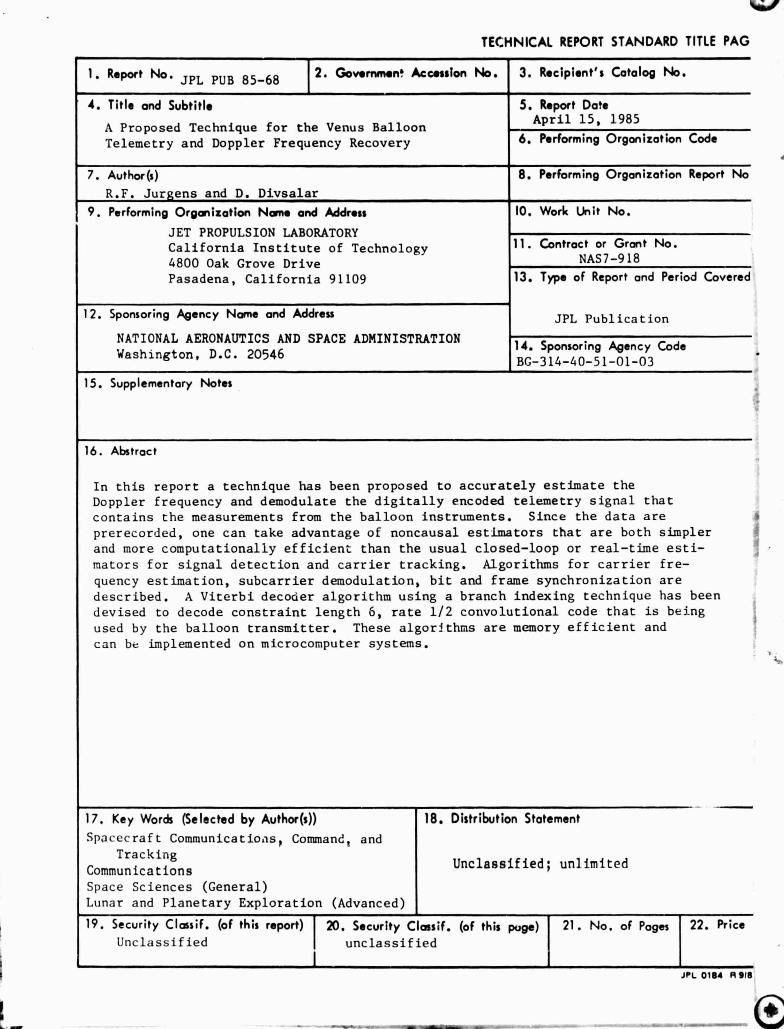
1. Report No. 2. Government Accession No. 3. Recipient ' s Catalog No.JPL PUB 85 -68
4. Title and Subtitle 5. Report DateApril 15, 1985
A Proposed Technique for the Venus Balloon6. Performing Organization CodeTelemetry and Doppler Frequency Recovery
7. Avthor(s) 8. Performing Organization Report No
R.F. Jur ens and D. Divsalar
9. Performing Organization Name and Address 10. Work Unit No.
JET PROPULSION LABORATORY11. Contract or Grant No.California Institute of Technology
4800 Oak Grove Drive NAS7-918
13. Type of Report and Period Covered
JPL Publication
Pasadena, California 91109
12. Sponsoring Agency Name and Address
NATIONAL AERONAUTICS AND SPACE ADMINISTRATION14. Sponsoring Agency Code
Washington, D.C. 20546BC-314-40-51-01-03
15. Supplementary Notes
16. Abstract
In this report a technique has been proposed to accurately estimate theDoppler frequency and demodulate the digitally encoded telemetry signal thatcontains the measurements from the balloon instruments. Since the data are
prerecorded, one can take advantage of noncausal estimators that are both simpler
and more computationally efficient than the usual closed-loop or real-time esti-
mators for signal detection and carrier tracking. Algorithms for carrier fre-
quency estimation, subcarrier demodulation, bit and frame synchronization are
described. A Viterbi decoder algorithm using a branch indexing technique has been
devised to decode constraint length 5, rate 1/2 convolutional code that is being
used by the balloon transmitter. These algorithms are memory efficient and
can be implemented on microcomputer systems.
17. Key Words (Selected by Author(s)) 18. Distribution Statement
Spacecraft Communications, Command, andTracking
CommunicationsUnclassified; unlimited
Space Sciences (General)
Lunar and Planetary Exploration (Advanced)
19. Security Classif. (of this report) 20. Security Classif. (of this puge) 21. No. of Pages 22. Price
Unclassified unclassified
4
.....r..,..,.^-- fir/ ..^
iii
1
1
s
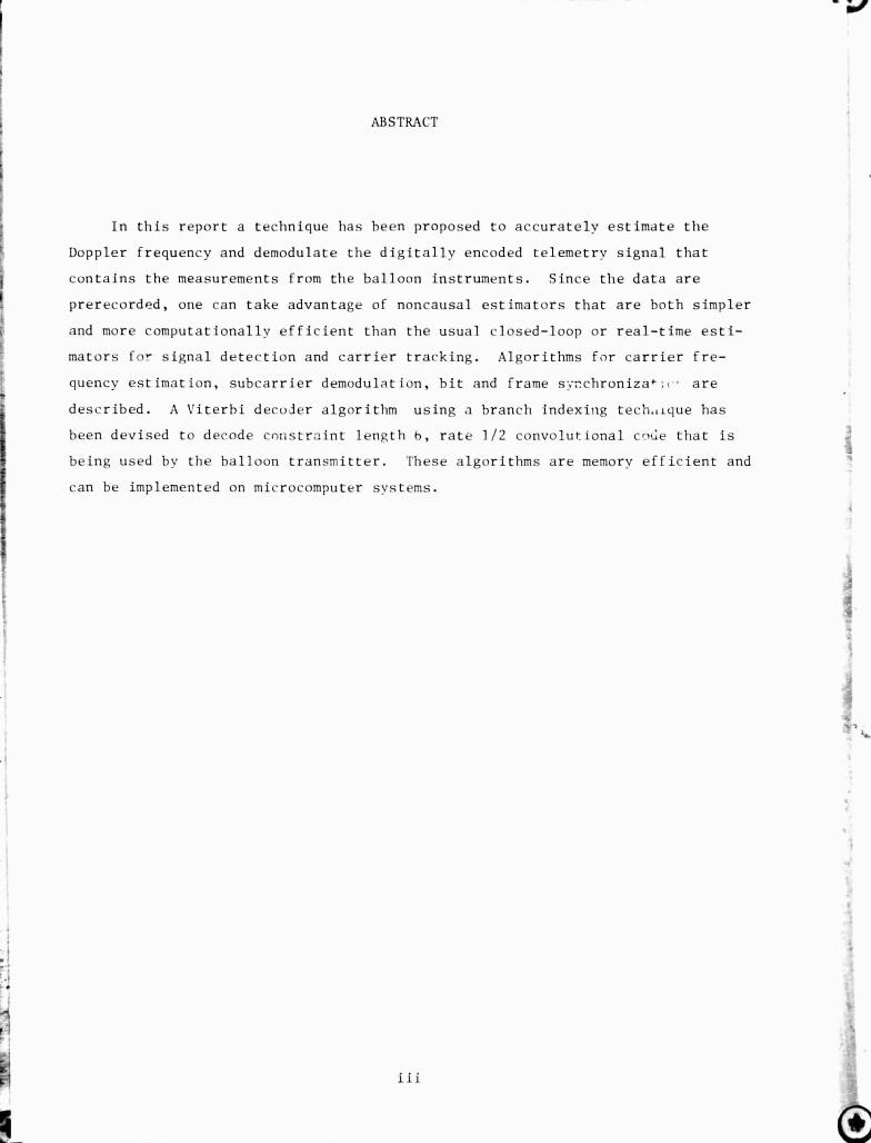
ABSTRACT
In this report a technique has been proposed to accurately estimate the
Doppler frequency and demodulate the digitally encoded telemetr y signal that
contains the measurements from the balloon instruments. Since the data are
prerecorded, one can take advantage of noncausal estimators that are both simpler
and more computationally efficient than the usual closed-loop or real-time esti-
mators for signal detection and carrier tracking. Algorithms for carrier fre-
quency estimation, subcarrier demodulation, bit and frame s_:r.chroniza-; • are
described. A Viterbi deco ,.ier algorithm using a branch indexing tech.,Ique has
been devised to decode constraint length b, rate 112 convolutional co(le that is
being used b y the balloon transmitter. -These algorithms are memory efficient and
can be implemented on microcomputer systems.
i
s
i-1*6
z O

t
t
CONTENTS
! 1. INTRODUCTION . . . . . . . . . . . . . . . . . . . . . . . . . . . . 1
I1. INITIAL. DETECTION TECHNIQUE . . . . . . . . . . . . . . . . . . . . 3
a. Determination of Filter Passband Shape . . . . . . . . . . . . . 3
b. Baseline Removal . . . . . . . . . . . . . . . . . . . . . . . . 4
e c. Threshold Detection . . . . . . . . . . . . . . . . . . . . . . 4
d. Carrier Frequency Estimation . . . . . . . . . . . . . . . . . . 6
III. DOPPLER RECOVERY AND THE EQUATION OF TIM1. . . . . . . . . . . . . . 8
a. Filtering and Data Reduction . . . . . . . . . . . . . . . . . . 8
b. Estimation of J-)puler Model . . . . . . . . . . . . . . . . . . 10
IV. CARRIER DEMODULATION . . . . . . . . . . . . . . . . . . . . . . . . 17
V. St'BCARRIER DEMODULATION . . . . . . . . . . . . . . . . . . . . . . 18
VI. BIT SYNCHRONIZATIoN . . . . . . . . . . . . . . . . . . . . . . . . 19
VII. FRAME SYNCHRONIZATION . . . . . . . . . . . . . . . . . . . . . . . 20
VIII. VITERBI DECODER . . . . . . . . . . . . . . . . . . . . . . . . . . 22
a. Code Structure . . . . . . . . . . . . . . . . . . . . . . . . 22
h. Code State . . . . . . . . . . . . . . . . . . . . . . . . . . . 24
c. Quantization . . . . . . . . . . . . . . . . . . . . . . . . . 24
d. Metric Quantization . . . . . . . . . . . . . . . . . . . . . . 26
e. Unquantized Metric . . . . . . . . . . . . . . . . . . . . . . . 27
f. Viterbi Algorithm . . . . . . . . . . . . . . . . . . . . . . . 28
g. Bit Error Rate Performance . . . . . . . . . . . . . . . . . . . 39
IX. CONCLUSION . . . . . . . . . . . . . . . . . . . . . . . . . . . . . 41
X. REFERENCES . . . . . . . . . . . . . . . . . . . . . . . . . . . . . 42
APPENDIX . . . . . . . . . . . . . . . . . . . . . . . . . . . . . . . . . A-1
^:< .;[?; vG PAGE, BLAND: NOT MMEDv
aI1
- - 0

CONTENTS (continued)
(01
'I
Figures
E ' 1. Baseband Filter for Carrier Separation . . . . . . . . . . . . . . 9
2. Linear Weights for Interpolation of Phase . . . . . . . . . . . 16
4
^3. Subcarrier Demodulator . . . . . . . . . . . . . . . . . . . . . . 18
e
4. Output Sample of Integrators in Subcarrier Demodulator vs. T 18sc
5. Bit S ynchroni-.^r . . . . . . . . . . . . . . . . . . . . . . . . . 19
6. Frame Synchronizer . . . . . . . . . . . . . . . . . . . . . . . . 21
7. Code Structure . . . . . . . . . . . . . . . . . . . . . . . . . . 22
1 8. Uniform I.-Level Quantizer lv'here TN Is Upper 'Threshold oftQuantization . . . . . . . . . . . . . . . . . . . . . . . . . . . 25
_ 9. Integer Code Symbol Metrics for L-Level Quantization . . . . . . . 26
10. Code Symbol Metrics for Unquantized Samples . . . . . . . . . . . 27
11. State Transitions Between Pair of States . . . . . . . . . . . . . 31ti
12. Bit Error hate Performance of Viterbi Decoder . . . . . . . . . . 40 f
a
1. Code Weight Distribution .
2. Typical Values for TH
3. Branch Metrics Computation
4. Branch Metrics Computation
5. State Transitions With Ass
. . . . . . . . . . . . . . . . . . . . 24
. . . . . . . . . . . . . . . . . . . . 26
for L-Level Quantization . . . . . . . 27
for Unquantized Samples . . . . . . . . 28
iciated Branch Indexes . . . . . . . . . 32
vi

nk a
IM
11 n
I. INTRODUCTION
The Venus Balloon (Vega) Mission is a joint French-Soviet-and US project to y
place two balloons on the atmosphere of Venus. The balloons will be tracked by
Very Long Baseline Interferometr y (VLBI) to determine their positions and veloci- to
ties on the disc of Venus. Besides this, the gondola contains an instrumentation
package that sends telemetry data directly to earth using an L-band transmitter.
This mission is described more full y in reference 111.
The scientific data recover y of the Venus Balloon mission requires accurate
estimates of the Doppler frequency of the balloon transmission as well as tits•
demodulation of the digitally encoded telemetry signal that contains the measure-
ments from the balloon instruments. Toward this end, the balloon signal has been
designed to provide an easy method to determine adequate starting; parameters from
this weak signal. Specificall y , an unmodulated carrier wave is transmitted at
the beginning and end of the data transmissions for a period of 30 seconds.
A known bit sequence follows the carrier wave such that the starting time
can be estimated accuratel y . To aid in carrier Lracking, through the frame,
4^' modulati, ,n is used such that h.tlf the transmitted power remains in the
carrier wave. The subcarrier wave is separated far enou}:h from the carrier that
I t
the information spectrum does not approach the carrier frequency; thus, it is
easy to f ilter the carrier out of the signal for accurate Doppler extracti011.
L.
The Doppler shift of the balloon transmission depends upon the balloon's
location in tale atmosphere and upon thv motion of the balloon within the atmos-
phere. As the balloon drifts across the disc of Venus, the Doppler shift should
drift from high to low frequency. The total drift should be constrained within
kHz. The width of the modulation spectrum requires an e:•:Lra 500 Hz. Thus a
total spectral widib of 2.5 kHz needs to be preserved if there is no a priori
knowledge of thu initial frequency. As Lhere is sotre a priori knowledge, probably
it is safe to preserve 2 kHz whi,h requires that rough1v 4k samples per second
*i
a:
be recorded. Eight or twelve bit samples are fully adequate as no appreciable
quantizing errors will exist, since the signal to noise ratio in the 2 kHz
bandwidth is well below unity. Telemetry transmissions occur at a minimum period
of one half hour. The total recorded telemetry data represents less than 109
unprocessed bits.
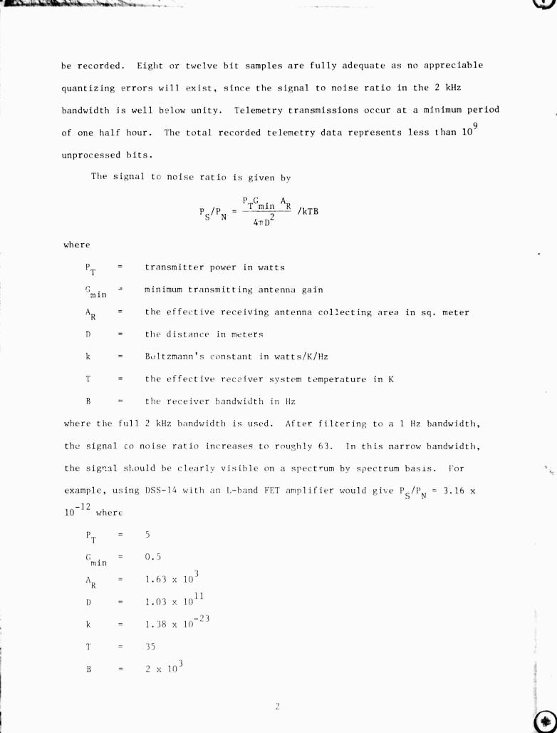
The signal to noise ratio is given by
pSN = [?T( .mi' A^ /
k'I'B
4-n D`
where
PT= transmitter power in watts
C =min minimum transmitting antenna gain
AK= the effective receiving antenna collecting area in sq. meter
P = the distance in meters
k = Boltzmann's constant in watts/K/Hz
T = the effective receiver system temperature in K
B = the receiver bandwidth in Ilz
where the full 2 kHz b;m dwidth is used. After filtering to a 1 Hz bandwidth,
they signal co noise ratio increases to roughly 63. In this narrow bandwidth,
the signal should be clearly visible on a spect rum by spectrum basis. Por
example, using DSS-14 with an I.-band FET amplifier would give 11
/ p' j = 3.16 x
10 -12 where
5
^, = 0.5min
A lj = 1.63 x 10³
U = 1.03 x 10¹¹
k = 1. 38 x I O-23
T - 35
2 x 10³
i
IO,.

r^!
11. INITIAL DETECTION TECHNIQUE
a. Determination of Filter Passband Shape
Prior to the arrival of the actual Balloon signal and periodically while no
signal exists, the receiver passband should be measured accurately. Since the
passband shape is determined by the offset baseband filter and any aliasing due
to the discrete sampling, it is not expected that the shape will vary signifi-
cantly over any time scale of interest to the detection of a single telemetry
frame. An accurate enough passband spectrum can be obtained by averaging 200 sig-
nal free power spectra to get roughly 7% statistics. If each spectrum uses 4096
samples, the time to acquire this average noise spectrum is 200 r, 4096 = 204.8 s or4000
about 3.4 minutes.
Procedure:
Using the signal free region of the recorded data, perform the Real Fourier
Transform (RFT) algorithm. (Details of the theory of the RFT have been supplied
as NASA Tech Brief No. NPO-11649.) The real Fourier transform results in place
of the data array that contained 4096 points. Next form the power spectrum from
these data. The power spectrum will result in N/2 + 1 points (2049) as follows:
The first point in the transformed array is the a 0 term, the second point is the
a N/2 term, the remain-ing N•-2 points are complex, thus a l = d 3 + 1 d4,
a 2 = d 5 + j d6 , a = d 2k+1 + i d2k+2 ..., aN/2-1 Li N-1 + j d N
. a0 = d + 1 01
aN12 = d 2 + 1 0 where a is it complex component of the transformed array and d
are the result of the RFT program.
To begin, clear the power array P which contains N/2+1 points. Next
accumulate 200 spectra points to this array by forming the power from the array,
where
Pn(k) Pn W + a k ak ; k = 0,...,N/2
r'
3

^l
Save the P array to use as a baseline reference to detect the unmodulated
carrier. Note that the standard deviation of the noise spectrum will be about
7% of the mean value.
b. Baseline Removal
Spectra measured during the carrier portion should contain a strong line at
the carrier frequency. Due to acceleration on the balloon, the carrier frequency
could vary by as much as 0.5 Hz/s but rather uniformly for periods as long as the
data transmission period. Thus it is not advisable to accumulate the spectra for
any appreciable period as smearing would result. The signal power spectra should
be determined in the same way as the noise power spectra. Let P s be a signal
spectrum resulting from a single RFT. Then the effects of the passband shape
can be removed by division.
Ps (k) + Ps (k)/Pn (k) k - 0, ...,N/2
C. Threshold Detection
The object of this section is to provide a way to automatically search for
the spectral line and to determine if a spectral line has been detected in the
present data frame. Let k and k .4100
represent the limits of the search where k
could start at zero and k/N
could range to N/2. Let there be M spectra containing
pure carrier. In reality a single spectrum is formed from 1.02 s of data, and
there are 30 s of pure carrier, so there will be roughly 29 such spectra. Let
L(n), 1 - n S M be an array that stores the location of the detected
line for each spectrum.
1
j
4
o^^
1- r- jcedure :
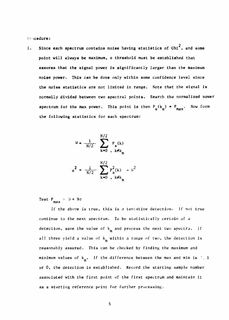
1. Since each spectrum contains noise having statistics of Chi t , and some
point will always be maximum, a threshold must be established that
assures that the signal power is significantly larger than the maximum
noise power. This can be done only within some confidence level since
the noise statistics are not limited in range. Note that the signal is
normally divided between two spectral points. Search the normalized power
spectrum for the max power. This point is then Ps(km) P max . Now form
the following statistics for each spectrum:
N/2
U . N/2 E P 5k-0 , kOkm
N/2
N/-2 1: s
k=0 , kOkm
Test P , U + 90max r•
If the above is true, this is a ten.ative detection. if not true
continue to the next spectrum. To be statistically certain of a
detection, save the value of km and process the next two spectra. ifi
all three yield a value of km within a range of two, the detection is
reasonably assured. This can be checked by finding the maximum and
minimum values of k . if the difference between the max and min is 1m
or 0, the detection is established. Record the starting sample number
associated with the first point of the first spectrum and maintain it
as a starting reference point for further processinV.
5

2. Beginning at this time reference, use the above procedure to fill the
array L(n) with the successive values of km . Process 29 spectra.
d. Carrier Frequency Estimation
The array L(n) contains the trace of the cw line as a function of time. It
is expected that this will form a straight line having a small slope. There is
some probability that bad estimates of k m exist. It is likely that these will be
widely separated from the main sequence of points. Thus it is necessary to
attempt to eliminate the bad points if they exist.
Procedure:
I. Find the mean of L. and mark all points deviating from the mean by
more than 5 by replacinp the value of L(n) with -1.
2. Find a line of regression by linear least squares that represents L(n).
Skip all points containing -1 in this analysis. The result of this
analysis is an equation that gives L - a x + b. In the above analysis,
the values of x should be the sample number. For example, x should
be associated with the center sample number for the first spectrum.
That is, x is sample number 2048 counting from the sample reference
number. In this way the variation of the instantaneous frequency can
be predicted relative to the reference sample number. Thus if i is
the sample number and iref is the reference sample number, the fre-
quency (in frequency number) Is given by
L - a (I - i ref ) + b
and
x (i ref - 1) +2 +nNI
6
v
.i
'i

where n is the spectrum number and L is a measure of frequency cell
number as a function of sample number. It is useful to know both
phase and frequency as a function of sample number where real time is
referenced to the first sample (i ref ). If SR is the sample rate and
N the number of samples in the RFT, then
SLet w(i) = 21 N [( i - i ref ) a + b]
t = (i - i ref )/SR
S
Then w(t) = 27 N [a S R t + b]
(t) =^ SN [a S R t 2 /2 + bt]
2°SR b 2-SK aThus w = N
and w =N —
3. Repeat the above procedure for the end-of-frame cw spectra. This
forms a second equation of frequency versus sample number. Let L A be
the first and L B the second, then some measure of frequency stability
over the data frame can be determined by evaluating the difference of
LA and 1. B at a point near the center of the frame. if this difference
is too large, it may be difficult to track the carrier through the
frame.
R
'.
7
ti
11

III. DOPPLER RECOVERY AND THE EQUATION OF TIME
a. Filtering and Data Reduction
All balloon motion relative to the center of Venus is unmodeled in the
frequency drifting of the first local oscillator. Thus it is important to know
the Doppler shift accurately to know the radial velocity and acceleration of the
balloon as well as to be able to demodulate the carrier wave. LA and LB give a
first order prediction of that Doppler, but furtner prediction may be carried
out by filtering out the sidebands and tracking the carrier through the frame.
The frame consists of 330 seconds of data, and there are 1.32 x 10 6 samples
through the frame. Since this is far too many to store in the computer memory,
it is important to perform some data reduction. We are interested in frequency
departures relative to our initial frequency line of regression. Normally,
departures of more than a few Hz from this line are unexpected (note each
frequency bin has a width of 4000/4096 = 0.9765 Hz). To get some bound upon
this, determine the maximum difference between ILA - LB I over the whole time
span. The width of the filter can be set at twice this value. Call this
bandwidth B. Note that the Nyquist sampling requires only 2B samples per second.
Since B will be only a few Hz, only four or five samples per second are required
to specify the carrier signal. Thus, roughly two thousand memory locations
are needed to store the information for the entire frame. This data reduction is
achieved by heterodyning the input signal ;samples) with a reference carrier
based on LA and filtering. The filter can be a simple running average of 1/2B
seconds of data; however, it is convenient to form complex samples at a rate of
1/B using a complex mixer. Figure 1 below shows the block diagram for a complex
mixer.
8
7

$1 C(i)
Figure 1. Baseband Filter for Carrier Separation
Procedure:
1. Determine B as discussed above.
2. Let T = 1/B. The number of samples to average in the filter is then
4000 T = M.
3. Beginning at the reference sample form the products
S i Cos[27r(wt + 2 t 2 )] t is time
andS i Sin[27r(wt + 2 t 2 ) ]
Then produce the average of M such samples such that
( k+1)2 + iref
C k = Si Cos [2-(wt + 2 t2)]2
+ iref
j L S i Sin [27(wt + 2 t2)]
4. Save C for further analysis.
P 9

b. Estimation of Doppler Model
In this section, we attempt to construct an accurate model of the carrier
wave to be used as a phase coherent reference for demodulation of the subcarrier
signal. This is essential to prevent the true carrier and the estimated local
carrier from forming a beat that modulates the subcarrier amplitude. The phase
coherent local oscillator is constructed from the carrier samples C k. The extent
to which the carrier model M k can represent the data depends upon many factors
such as the signal to noise ratio, the phase stability of the transmitter, the
motion of the balloon, the atmospheric turbulence and many other stochastic
errors and unmodeled effects. Thus it is not possible to know a priori the level
to which coherence can be established. For that reason, it is necessary to know
when the carrier tracking loop is locked as tightly as possible. A simple
criterion is to establish whether the estimated carrier signal has fallen signi-
ficantly below the estimated incoherent power level. Thus we attempt to lock the
carrier model to the carrier samples as tightly as possible by narrowing the
effective bandwidth until the signal level begins to drop. The effective band-
width is controlled by the duration of the data span used in the processing.
Increasing the span to 30s should be possible most of the time unless the balloon
is undergoing severe turbulence or accelerations.
Procedure:
Nonlinear Least Squares Regression
Let the carrier signal model be given by
j(O + wtk - w/2t2"k=Ae
where
A is an amplitude coefficient
10
- 7--- '^ r Mwys^

M^
AV
0 is an initial phase reference
t is the time of the kth sample and k is centered in the span of data
w is the frequency
w is the rate of change of frequency
Let the error between the measured samples and the model be given by
NE = E Wk IOk - Mkl2k--N
where Wk is a set of weights that are normally set equal to the reciprocal of the
noise variance, and 2N+1 is the number of samples in 30 seconds. In this case
the weights can be set equal to unity unless the true covariance matrix is needed.
We desire to minimize E by adjusting A, ^, w, and w. Let x represent the vector
A, 0, w, w and Ax represent a vector of small corrections to x.
Ax = [AAA 0, Aw Aw]
Then
aMk aMk j(^ + wtk + w/2tk)
DA ax - e1
aMk r aMk j(m + wtk + w/2tk)
a¢ ax j A e
aMk aMk j(^ + wtk + w/2tk
aw ax
)
- J A tk e
aMk aMk 2 j(O + wt k + w/2t2
aw = ax4j A tk/2e
11
^ - r

T F
A minimum in a requires that
ac - 0ax
Thus
N a *
E2 Re jWk(Ck - Mk)
axk^• 0 i = 1,...,4
k---Ni 1
Mk may be expanded about the initial value of x. If we substitute only
the linear terms of the series for M k, we arrive at the normal equations. Let
4 aMk
Mk 2' Mok + E axj axj
J - 1 _
I xj xoj
'18
Na * 4 N
Er ^ r r2 Re Wk (Ck Mok) ax • E E
k--N J-1 k--N
evaluate
*aMk aNk
Z Re Wk ax
j ax, AX
'Mk at x•xax o
Then
The normal equation forms four equations with four unknowns where Oxj are
i the unknowns. This solution must be iterated until the Ax are suitably small.
Thus the next estimate of x - x + Ax. The meaning of suitably small is either
defined from the limits of the measurements as defined by the covariance matrix
(the inverse of the normal equation matrix) or by what is reasonable. Reasonable
12

in this case is determined by theoretical limits or by how much error we can stand.
In general a phase error of 10° is about as large as acceptable. This constrains
A# < 0.17, Aw < 0.01 and Aw < 0.0015 for a 30s span. In general, the iteration
should be driven to about a tenth of these values.
Accurate starting estimates are usually required to begin the nonlinear least
squares regression analysis. The prediction equation given by LA should normally
determine the frequency to an accuracy slightly better than 0.5 Hz. In such a
case the maximum integrated phase error approaches 360° in two seconds. The least
squares procedure requires that the phase error be less than 180° and preferably
less than 90° over the data span if convergence is to be assured. Assuring the
phase error is small enough either requires that the preliminary estimates of w
and w are adequate for the time span considered qr that the time span is short
enough. If the time span is too small, the signal to noise ratio will be too
small for adequate detection. Since most of the w term has been heterodyned out
by the LA model, it normally can be initialized to zero. Determination of w can
be dune in several ways, each of which has merit under certain conditions. We
suggest the following possibilities:
1. Under normal conditions, the NLLSR can be used with a short span of
data (about Is). Once convergence is established, the span can be
doubled using the new estimate of w. This can be continued until the
30s span either converges or the estimate of A begins to drop, indicating
inadequacy in the model or phase incoherence of the signal.
2. A sequence of is estimates can be made over the 30s data span using
NLLSR. The resulting w then can be used to form a linear equation of
frequency giving w and w as starting parameters. This procedure has
been tested and works well if the signal to noise ratio is adequate.
13

3. This last procedure may be useful if convergence cannot be obtained
using 1 and 2 above. Use the complex fast Fourier transform (FFT) to
form the power spectrum of the Ck 's. The span of data could extend to
30s giving 1/30 Hz resolution. A peak detection scheme similar to that
of Section IIc can be used to find the maximum power and its location.
This procedure will not work if w is too large, but does work for
smaller signal to noise ratios than procedure 2.
A first estimate of AeJ ^ can be formed by simple correlation of the model
with the data Ck.
1 N
-j (wt + 2 t2
Ao 2N+1 E Ck ek=-N
Thus
A= I oIArctan (Im A/Re A)
As we progress through the data, it is best to determine the starting values from
the results of the previous data. However, A and # can always be computed quickly
from the procedure above.
Experimentation with some carrier models has shown that some procedure for
2detecting nonconvergence is necessary. A suitable estimate is to assure that A
does not fall significantly below the estimated carrier power level. An estimate
of the incoherent power is given by P where
N 2_ 1
P2N+1 ICkI - N
k=-N
N is an estimate of the noise power which can be formed from the original signal
statistics by noting that the power in the 2 kHz band is mostly noise. Thus the
f.
14

.s
15
M
value of N can be related simply to the statistics of S i by noting that M samples
of the original signal were added together and the gain of the complex mixer is
1/2 per side.
K^ 2 1
E 2
N s M es M 2K+1 Sii--K
Here a2 is the variance of the samples, S i in the data span currently being
analyzed. This assumes S i are zero mean and nearly white.
The results of the above analysis provide a series of equations for estimat-
ing 0(t) that are valid over a 30 second strip of data. The 30 second spans are
formed every 15 seconds. These data are intrinsically valuable as scientific
output and are used for the carrier demodulation discussed in the next section.
Clearly, the previous operations provide a great data reduction in specifyingi7i
the phase function since each 30 second strip of data is represented by four b
numbers and there are only 22 such strips over the data frame. f.
The above procedure provides no guarantee that the phase is continuous across
the thirty second boundaries. However, since the equations are valid over a 15i
second period overlapping consecutive strips, it is possible to force the phase toi.
be continuous by using a weighted combination of two adjacent equations to form
the phase function. Figure 2 below shows the form of the weights.C.,

#k+1
e 2. Linear Weights for Interpolation of Phase
Lon is formal as shown in Figure 2 where
.tx_tk
Wk(tx) ati At t
k+l - tk
f(tx )
(1-W k (t X))f k
(t x ) + Wk(tx)^k+l(tx)
^k(tx) ' wktx + 2 t 2x
and wk,wk are from least squares regression. Thus the continuity of phase across
the boundaries is assured.
16

y ^
IV. CARRIER DEMODULATION
The carrier demodulation is easily carried out using the phase function of
the previous section. If we presume that the binary (square wave modulation) is
B(t), then the modulated signal is of the form
j f n 14 B(t) + e(t)]SW - Se
where B(t) - +1 and S is a real amplitude weight. e(t) is presumed to be composed
of drifts in the transmitter and Doppler shift due to balloon motion. e (t) esti-
mates both phase components, thus the recovered modulation r(t) is given by
—j e(t)
r(t) - S e
9(t) ¢(t) + wAt + 2 t2
*Note 1
When 8 - ed is small as it should be,
r(t) m S 2+ j sin 4 B(t)
Note that verification of proper phase demodulation can be checked easily by
simply averaging r(t). Since B(t) is zero mean, only the real part of r(t)
should remain finite. Note that the modulation is contained in the imaginary
part of r(t) and has an amplitude of f2 S.
*Note 1
SW is the original sample set beginning 12 seconds after initial detection,
thus this is 48000 samples past iref'
8(t) is then defined at the total phase
at that time. e(t) must be composed of the original phase due to LA and the
departures from LA given by @(t) where wA and OA are from LA (See page 7).
17

,l
V. SUBCARRIER DEMODULATION
First note that between times 31-3/8 sec and 34-1/4 sec we have an all zero
sequence. Therefore there are no transitions in symbols. (Look at the output
symbol ;rquence of convolutional code for frame sync inputs.) Therefore we can
demodulate the subcarrier and estimate the phase of subcarrier as shown in Fig. 3.
In Figure 4 the output samples of the integrators in subcarrier demodulator are
shown as a function of '[sc.
Sin (YK t1)
32 it, s 34 i^
Nit) r(q do [Y^(►^ - TK)^ Ca (W 8C ^')
Y(')
^ sfi
t
)t' ATs(+K)-C
32 s34
Fig. 3 Subcarrier Demodulator
A TS(T,,) ATK f ^K 1
T 22 1 1I0 1
TK TKI
-A
C A T,(TK) ATK T 3TK1 2 a
TK
.A
Fig. 4 Output Samples of Integrators in Subcarrier Demodulator vs. T ' }sc
18 ^`

IFB?O and C < 0Tm
T5C x C
SC 4(C-B)
TSC (C + 2B)
4
IFB<O and C < 0 TSC^ 4(C+B)
Sc_ (3C - 2B)
IFB<O and C ? 0tSCa
T
4(C-B)
IF B 0 and C > 0TSC -
TSC_(3C + 4B)
4(C+B)
after finding T SC we can shift the whole subcarrier signal by T SC (delay by TSC)'
Then we can demodulate the whole data frame by the subcarrier to get data samples
d(ti).
VI. BIT SYNCHRONIZATION
The bit synchronizer is shown in Fig. 5.
DATA DETECTOR TRANSITIONDETECTOR
kN+N+kxk
+1
•1
rUll
kN+—+tYk Ik ^.
I•kN-N+i+Zk
k0+M
1 ^ ZkM k-k0+1
t
Fig. 5 Bit Synchronizer
Let d(t i ) be data samples. Suppose during one symbol time there are N samples
d(t i ). In upper branch of Fib;. 5, we sum the N samples d(t i ) starting at time
kN + 1 + i (- 2 < - --2). Next we detect the sign of symbol. by passing through
19
i

a sign (-) function
1 ; x > 0
sign (x)
1-1 x < 0
Next we detect the transition in consecutive symbols a by finding one-half of
difference between consecutive detected symbol signs. If I 0 means there is
ro transitions, Ik + 1 means there is a transition. If Ik + 1 then we have
symbol transition from + 1 to - 1 and if I k « - 1, then we have symbol transition
from - 1 to + 1.
In lower branch in Fig. S we sum N samples d(t i ) starting at time kN - 2 + 1
+ 6. The result is sample Y k. Vle multiply Y by I to gat Zk. We repeat this
operation It times (11 a 60), starting at k - k 0 where time k 0 N is roughly at the
beginning of (30 - 42 sec) interval. Next we find the result of the average
of all H samples z as E. Now if c is positive we increase 6; if c is negative
we decrease 6. We repeat the whole operation until we get smallest c possible.
VII. FRAME SYNCHRONIZATION
We get the smallest possible c from bit synch. We store all detected
symbols a in a shift register. Next we compare the pattern of symbols that we
have at the output of encoder with contents of shift register. We shift this
pattern until we match the pattern with the content of shift register with
minimum number of discrepancies. Minimizing a in Fig. 6 can result in frame
sync, where b e(0,1) is related to a by
1 - akb - 2
and ®+ is exclusive OR.
*V
20

0
^, 9
PATTERN
1
i
Fig. 6 Frame Synchronizer
The input frame synchronization bits to the convolutional code during the
time interval (30-42) seconds are
17(0), 5(1), 3(0), 2(1), 1(0), 3(1), 1(0), 1(1), 1(0), 1(1), 4(0), 1(1),
2(0), 1(1), 1(0), 2(1), 2(0).
The corresponding output pattern of frame synchronization symbols of convolutional
code is
10(X), 24(0), 2(1), 2(0), 1(l), 1(0), 1(1), 5(0), 2(1), 1(0), 2(1), 1(0)
2(l), 1(0), 1(1), 1(0), 2(1), 1(0), 3(1), 1(0), 3(1), 7(0), 3(1),
3(0), 3(1), 1(0), 2(1), 1(0), 2(1), 3(0), 2(1), 1(0), 1(1).
Where the number in front of parentheses indicates the number of consecutive
bits shown in parentheses, the X means unknown bit. The contents of encoder
at time 42 is:
IN/UT
0 0 1 1 0 ^
^ JINITIAL STATEor ENCODER
214'

SHIFT REGISTER
T
OUTPUT
+,
VIII. VITERBI DECODER
This section explains the Viterbi decoder algorithm for a constraint length
K - 6, code rate r = 1/2 convolutional code. The code is shown to be a trans-
parent convolutional code. t The weight distribution of the code has been computed
by numerical analysis. The code state table, received sample quantization,
metric quantization, and Viterbi algorithm using a branch indexing technique is
explained in detail. The theoretical bit error performance of the code and the
simulation results of this Viterbi algorithm is given.
a. Code Structure
ConE 'er a K = 6, r = 1/2 convolutional encoder which is illustrated in
Figure 7.
Figure 7. Code Structure
rThe code has been provided by mission as in Fig. 7 without any further inorma-tion. The description of code was not available in the literature.
22
I
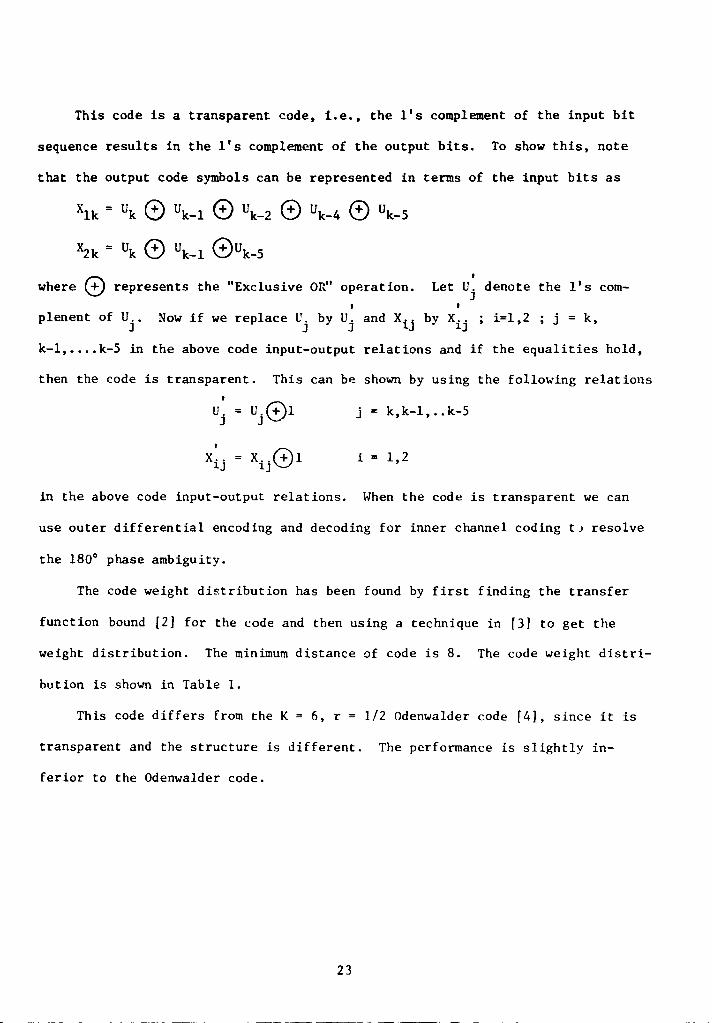
This code is a transparent code, i.e., the 1's complement of the input bit
sequence results in the 1's complement of the output bits. To show this, note 4
that the output code symbols can be represented in terms of the input bits as
Xlk = Uk 6 Uk-1 (D Uk-2 +O Uk-4 +O Uk-5
X2k = Uk O Uk-1 OUk-5
where +D represents the "Exclusive OR" operation. Let U ' the 1's com-
plenent of Uj . Now if we replace U by U and Xij by Xij ; i=1,2 ; j = k,
k-1,....k-5 in the above code input-output relations and if the equalities hold,
then the code is transparent. This can be shown by using the following relations
U = Uj (Dl j = k,k-l,..k-5
Xij = Xi .JOI i = 1,2
in the above code input-output relations. When the code is transparent we can
use outer differential encoding and decoding for inner channel coding tj resolve
the 180° phase ambiguity.
The code weight distribution has been found by first finding the transferr
function bound [2] for the code and then using a technique in [3] to get the
weight distribution. The minimum distance of code is 8. The code weight distri-
bution is shown in Table 1.
This code differs from the K = 6, r = 112 Odenwalder code [4], since it is
transparent and the structure is different. The performance is slightly in-
ferior to the Odenwalder code.
23 ;
y -r 4a -
__ ____
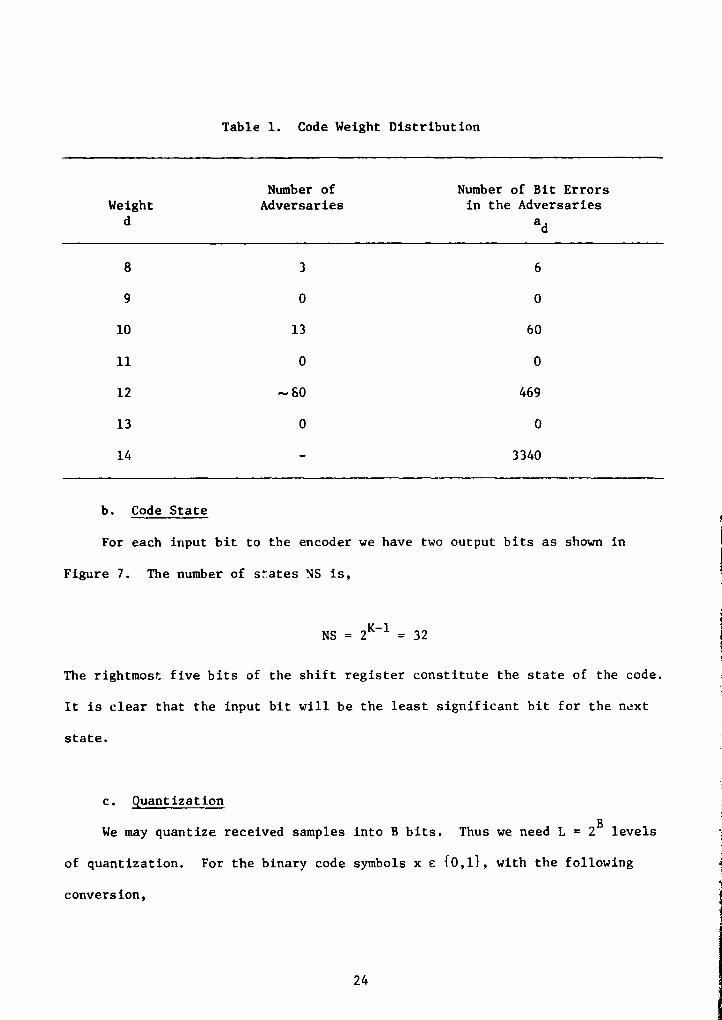
Table 1. Code Weight Distribution
Number of Number of Bit ErrorsWeight Adversaries in the Adversaries
d ad
8 3 6
9 0 0
10 13 60
11 0 0
12 —60 469
13 0 0
14 - 3340
b. Code State
For each input bit to the encoder we have two output bits as shown in
Figure 7. The number of s`:ates NS is,
NS = 2K-1 = 32
The rightmost_ five bits of the shift register constitute the state of the code.
It is clear that the input bit will be the least significant bit for the next
state.
c. Quantization
We may quantize received samples into B bits. Thus we need L = 2 B levels
of quantization. For the binary code symbols x c {0,1), with the following
conversion,
24
^' t

OUTPUT (QUANTIZATION LEVELS)
0 4 1
1 4-1
we can assign integers 0 through L-1 to the quantization levels, as shown in
Figure 8.
- p-
INPUT :r
(RECEIVED SAMPLE)
Figure 8. Uniform L-Level Quantizer Where TH is Upper Threshold of Quantization
25

Table 2 shows some typical values for TH assuming the noise samples are
normalized to have a unit variance.
Table 2. Typical Values for TH
L TH ! (2 - 1)A*
a
2 0
0 1
8 1.7
16 2.3
32 2.7
64 3.1
128 3.5
256 3.8
*A is threshold spacing.
d. Metric Quantization
Figure 3 shows integer code symbol metrics for L-level quantization.
LY QUANTIZATION LEVELSx 0 1 2 ................. . L-2 L-1
0CODESYM80l
1
Figure 9. Integer Code Symbol Metrics for L-Level Quantization
The branch metrics can be computed from Table 3.
R
L-1 L-2 L•3 .................. 1 0
0 1 2 ................... L-2 L-1
26

Table 3. Branch Metrics Computation for L-Level Quantization
Branch Index Branch Code Symbols Branch MetricIB s1 :2 LB
1 0 0 2(L-1) - LY1 - LY2
2 0 1 L-1 - LY1 + LY2
3 1 0 L-1 + LY1 - LY2
4 1 1 LY1 + LY2
The IB's are the branch indexes associated with the various distinct branch
symbols. For example for a branch with code symbols 10, IB - 3.
e. Unquantized Metric
If we do not use quantization for the received samples, then the code
symbol metrics can be computed from Figure 10, and the branch metrics are
t.computed from Table 4.
X RECEIVED SAMPLE
r
01 r
CODE SYMBOL
1 1 -r
Figure 10. Code Symbol Metrics for Unquantized Samples
27
a
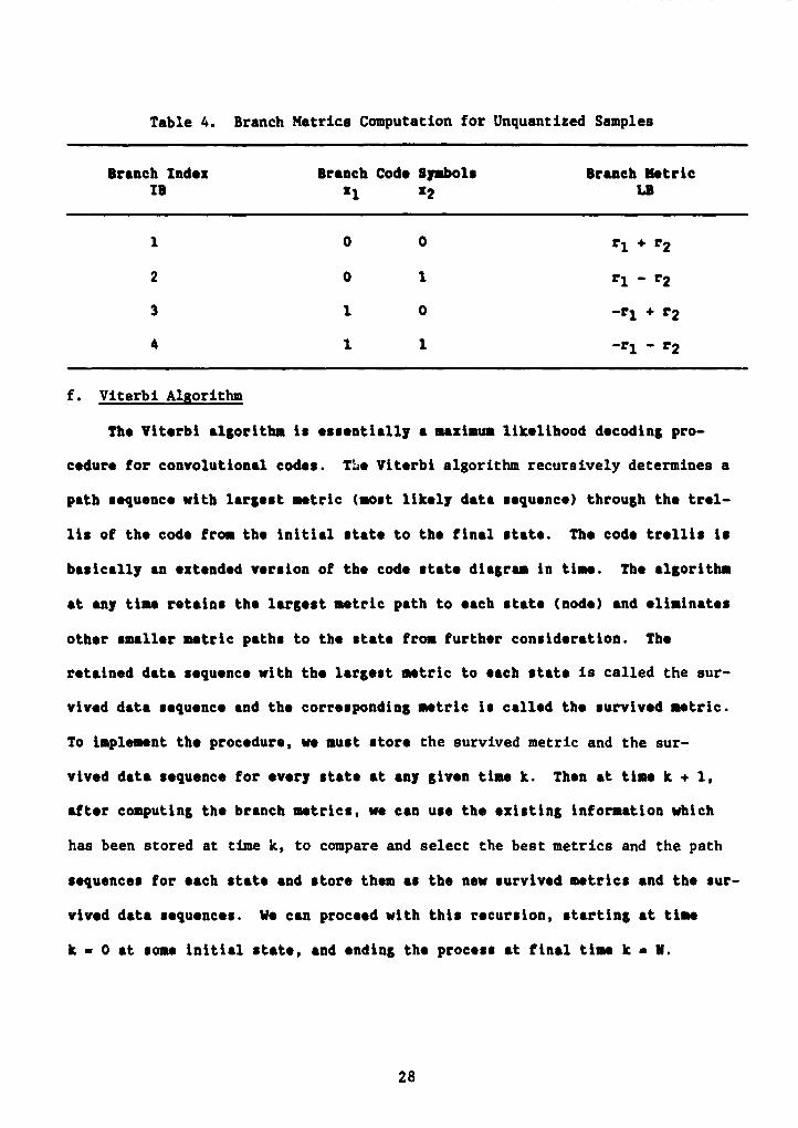
Table 4. Branch Metrics Computation for Unquantized Samples
Branch Index Branch Code Symbols Branch MetricIB xl 12 LB
1 0 0 rl+r2
2 0 1 rl - r2
3 1 0 -rl + r2
4 1 1 -rl - r2
f. Viterbi Algorithm
The Viterbi algorithm is essentially a maximum likelihood decoding pro-
cedure for convolutional codes. TLe Viterbi algorithm recursively determines a
path sequence with largest metric (most likely data sequence) through the trel-
lis of the code from the initial state to the final state. The code trellis is
basically an extended version of the code state diagram in time. The algorithm
at any time retains the largest metric path to each state (node) and eliminates
other smaller metric paths to the state from further consideration. The
retained data sequence with the largest metric to each state is called the sur-
vived data sequence and the corresponding metric is called the survived metric.
To implement the procedure, we must store the survived metric and the sur-
vived data sequence for every state at any given time k. Then at time k + 1,
after computing the branch metrics, we can use the existing information which
has been stored at time k, to compare and select the best metrics and the path
IJsequences for each state and store them as the new survived metrics and the sur-
vived data sequences. We can proceed with this recursion, starting at time
k - 0 at some initial state, and ending the process at final time k - V.
ti
28

4^
Finally we choose the data sequence with largest metric among all states at time
k - N as the decoded data sequence.
In practice since N is usually large, the amount of storage needed to
retain the survived data sequences is large. Therefore if M is very large, it
is necessary to truncate survived sequences to some length m. However it can be
shown that there is a high probability that all survived data sequences at time
k will have identical data bits very far back from the present time k. This
suggests that if the algorithm stores enough of the past data bits of each of
the 32 survived sequences, then the oldest bits on all stored data sequences
will be identical. Our simulation has shown that we only need to store m n 36
most recent bits of the survived data sequences; in this case the effect on per-
formance is negligible. Then the algorithm outputs the oldest bit in the sur-
vived data sequence at state number 1, as the hard decoded bit. Another practi-
cal consideration is metric overflows. Since the survived metrics grow in time,
to prevent a possible overflow, it is necessary to renormalize the survived
metrics from time to time. As follows we explain the algorithm in detail.
I. Definitions:
Hk(J) . Survivor metric at state number J at time k.
Ok. Array containing the survived metrics at time k, i.e.,
Hk=(Mk(1),Mk(2)...... Mk(32))
LB(IB) . Branch metric corresponding to the branch code symbols
x and x2 , indexed by IB
Array of branch metrics, i.e.. ^B .
(LB(1),LB(2),LB(3),LB(4))
Sk(J) : State number J; J = 1. 2,..... 32, at time k
29

^ JIyk' : Array of the m most recent bits of the survived data
sequence, terminating at state J at time k
Mok : 36 x 32 matrix that stores all arrays ^1c
M; J 192,
• 36..., 32 at time k
ak+1 3:o x 32 w-,trix that stores all arrays !lk+1.36W;
J - 1,2,...., 32 at time k+i
Array of all branch indexes from state number J to state
number 2J - 1, for J - 1, 2,...., 16
L1 Array of all branch indexes from state number 16 + J to
state number 2J - 1, for J n 1 9 2,...., 16
Array of all branch indexes from state number 16 + J to
state number 2J, for J - 1, 2....., 16
j,^• Array of all branch indexes from state number J to state
number 2J, for J - 1. 2....., 16
Note that since the first and the last stages of the shift register are
connected to the MOD 2 adders. then
J& - kQ and Ll' - kI
2. State Transitions
For a given J; 1 :S J < 16, the state transitions are shown in
Figure 11, where IB f IB'. All state transitions associated with the branch
indexes are shown in Table 5. Note that when we use branch indexing we need
only to compute 4 metrics each time rather than computing all metric branches.
Therefore branch metric computation is almost independent of number of states.i
30

7W
Figure 11. State Transitions Between Pair of States
I
31
lO

32
Table 5. State Transitions With Associated Branch Indexes
Sk(J) ak^lt?J-1)
Is
1 1 1
2 3 4
3 S 3
4 7 2
S 9 1
6 11 d
7 13 3
a 1S 2
9 17 3
10 19 2
11 21 1
12 23 d
13 25 3
16 27 2
is 29 1
16 31 e
+t1
ItAk
.,
a
i
^a

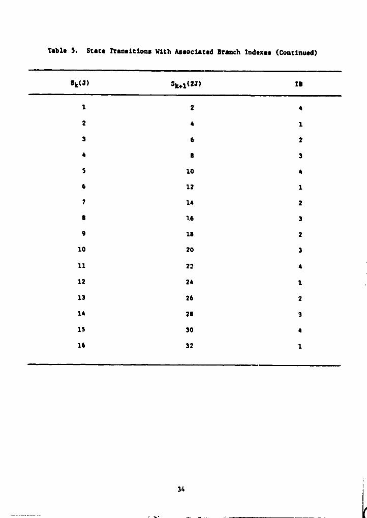
Table S. State Transitions With Associated Branch Indexes (Continued)
A
ak(16+J) Sk♦1(2J-1) is
17 1 4
1e 3 1
19 S 2
20 7 3
21 9 4
22 11 1
23 13 2
24 15 3
25 17 2
26 19 3
27 21 4
28 23 1
29 25 2
30 27 3
31 29 4
32 31 1
33
,+ i
With Associated Branch Indexes (Continued)
sk(J) gk♦1(2J) IB
1 2
2 4 1
3 6 2
s 3
S 10 e
6 12 1
7 14 2
s 16 3
9 is 2
10 20 3
i
22 t Y
24 1 ..
26 2
a.^2s 3
30 4 *,
32 1
34 I
V - jj ^., •AW

Table 5. State Transitions With Associated Branch Indexes (Continued)
14
Sk(16+J) Sk+1(2J)
'j 17 2
is
19 6 3
20 8 2
21 10 1
22 12 4
23 14 3
24 16 2
25 is 3
26 20 2
27 22 1
28 24 4
29 26 3
30 28 2
31 30
32 32 4
47
35
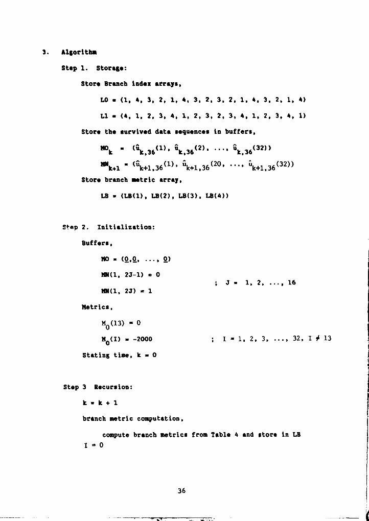
3. Algorithm
Step 1. Storage:
Store Branch index arrays,
LO = (1, 4, 3, 2, 1, 4. 3, 2, 3, 2, 1, 4. 3, 2, 1, 4)
L1 = (4, 1, 2, 3, 4, 1, 2, 3, 2, 3, 4, 1, 2, 3, 4, 1)
Store the survived data sequences in buffers,
no (uk.36(1). ak,36 (2). .... ii k.36
"Nk+l s ("k+1,36(1)' "k+1,36(20' " " k+1,36 (32))
Store branch metric array.
LB = (LB(1). LB(2), LB(3), LB(4))
i
e+ep 2. Initialization:
Buffers,
MO = (0.0. ..., 0)
MM(1, 2J-1) = 0
Mil(1, 2J) = 1
Metrics,
MO (13) 0
MO(I) _ -2000
Stating time, k = 0
; J = 1, 2, ... , 16
; I = 1, 2 9 3, ... , 32, I # 13
Step 3 Recursion:
k = k + 1
branch metric computation,
compute branch metrics from Table 4 and store in LB
I=0
36

Step I=I+1
Survived metrics,
Mk (2I-1) - Max j[Mk-1(I) + LB (LO(I))],
[Mk-1 (16+I) + LB(Ll(I))]^
Mk (2I) - Max j[Mk-1 (I) + LB(Ll(I))],
[Mk-1 (16+I) + LB(LO(I))]^
Select the survtved sequences from MO k-1 , add selected bit "0"
or "1" to it, store in scratch buffer MN
If Mk (2I-1) = Mk-1 ( I) + LB(LO(I))
then MN (J+1, 2I-1) = MOk-1 (J, I) J 1, 2, ..., 35
If Mk (2I-1) - Mk-1 ( 16+I) + LB (LO(I))
then MN (J+1, 2I-1) = MO k-1 (J, 16+I) J = 1, 2, ..., 35
If Mk (2I) = Mk-1 ( I) + LB(Ll(I))
then MN (J+l, 2I) = MO k-1 (J, I) J 1, 2, ..., 35
If Mk (2I) = Mk-1 (I) + LB (LO(I))
then MN (J+l, 2I) = MOk-1 (J, 16+0 J = 1, 2, ..., 35
If I < 16 go to step 4
restore MN into MO
MOk (I,J) = MNk (I, J) I = 1, 2, ..., 36
J = 1, 2, ..., 32
The decoded bit at time k is
MOk (36, 1)
f
4
37

- 1
Normalisation of survived srtriess
Find the largest NO); J - 1. 2s ...s 32 and call it MXH, then
Mk(J) • Mk(J) - M ; J - 1 9 2 9 .... 32
call node synchronisation algorithm and store the result in NOD.
If K < N go to step 3
Otherwise, choose the largest metric among all the survived metrics at
k - N. The corresponding data sequence in the buffer MO is considered
as the final decoded sequence.
38
4W^. _ n';1 `,rte

g. Bit Error Rate Performance
From our analysis using Table 1 for weight distribution of code and then
using union bound we can approximate [3] the bit error rate P b as*
Pb ow 3 erfc 4 Mb + 30 We S Nb + 250 erfc 6 Mb + 1670 We ( 7 N b )
0 0 0 0
where
Eb is bit signal to noise ratio andN 0
2
erfc(s) _ 2 e t
dt
1rfxm
Figure 12 gives the theoretical performance of this algorithm and the
simulation results. The .25 dB loss in simulation with respect to theoretical
result is due to infinite bit quantization that we assumed in theoretical result,
and it is due to path memory truncation and metric quantization in the software
algorithm.
i
1
i
*Theoretical upper bound is [2]
4E dEb
P < 1/2 erfcF
e+ NOEa e 2N
0 )b —
d
where ad are coefficients in tr •nsfer function bound [2]. The first few
are given in Table 1.
39

•^.l
1.00 i.SO e.00 8.50 3.00 3.50 4.00 4.50 5.00 5.50 6.00
`Wn
ccCK
0CKOCW
F-H0
Ile—
BIT SNR (DB)
Figure 12. Bit Error Rate Performance of Viterbi Decoder
40

IX. CONCLUSION
The algorithms and subroutines developed in this study are suggestions for
constructing an actual data processing program and may require some further
optimization.
Simulations of the carrier tracking loop have indicated that the least-
squares procedure for finding w and w may not converge if the starting parameters
are not close enough to the actual w and w, if the noise is too large, or if the
phase fluctuations are so large that the 30 second coherence span is too long.
Normally if the carrier extraction is successful, the subcarrier extraction, bit
and frame synchronization proceed smoothly. Simulations of the decoding algo-
rithm are in good agreement with the theoretical performance. Detailed analyses
of the statistical performance of the subcarrier demodulator has not been carried
out, but the techniques used for signal processing should not produce any signi-
ficant degradation from the theoretical values. For this reason, the major un-
certainty in the decoding is associated with the carrier extraction and the
processes that could cause unmodeled phase modulation of the carrier wave.
41

m.. J0.
X. REFERENCES
[1] P.A., Preston, J.H. Wilcher, and G.T. Stelzried, "The Venus Balloon Project,"
TDA Progress Report 48-80, pp. 195-201, October-December, 1984.
[2] Viterbi, A.J. and Omura, J.K., "Principles of Digital Communication and
Coding," McGraw-Hill, 1979.
[3] Divsalar, D.. "Performance of Mismatched Receivers on Bandlimited Channels,"
Ph.D. dissertation, University of California, Los Angeles, 1978.
[4] Odenwalder, J.P., 'Optimal Decoding of Convolutional Codes," Ph.D. disser-
tation, University of California, Los Angeles, 1970.
Y•
42 1
j fir/ • i

ti
IWO
f:
i
i
APPENDIX
SUBROUTINE SETUPC****w********+►*** SET UP FOR V I TERB I DECODER **+ ►*+►+►****+► +►****CC M IS VECTOR OF STATE METRICS CC LO IS INDEX VECTOR OF ALL STATE TRANSITICNS SUCH AS J->2J-1 CC ;J-1,2,.....,16. CC L1 IS INDEX VECTOR OF ALL STATE TRANSITIONS SUCH AS CC 16+J->2J-1; J-1, 2, ...... 16. CC NOTE :INDEX VECTOR OF ALL STATE TRANSITIONS SUCH AS J->2J CC IS Ll. CC INDEX VECTOR OF ALL STATE TRANSITIONS SUCH AS CC 16+J->2J IS L0. CC MO IS 36*32 MATRIX WHICH STORES ALL BEST PATHS TO 32 STATES,CC IT ONLY KEEPS PATHS WITH LENGTH 36.THE 37TH BIT CAN BE CC REGARDED AS HARD DECODED BIT. CC MN IS 36*32 SCRATCH MATRIX. C
COMMON/LA1/LO(16), Li (16), M(32), MO(36, 32), MN(36, 32)DATA LO/1,4,3,2,1,4,3,2o3,2,1,4,3,2,1,4/DATA L 1 /4, 1, 2, 3, 4, 1, 2, 3, 2, 3, 4, 1, 2, 3, 4, 1
C INITIALIZATIONDO 5 J-1,32DO 5 1-1,36
5 MO( I, J)-0DO 10 1-1,16I1-I+I-1I2-I+IMN(loll)-0
10 MN(1, I2)-1C ASSUME ENCODER IS IN :STATE K 13
DO 20 I-1,3220 M(I)--2000
M(13)-ORETURNEND
CC
SUBROUTINE DECODE(KTMI, LY1, LY2, L, KTMO, KOUT)C THIS SUBROUTINE IS VITERBI DECODING ALGORITHMC KTMI IS INPUT TIMEC KTMO IS OUTPUT TIMEC LY1 AND LY2 ARE QUANTIZER OUTPUTSC L IS NUMBER OF QUANTIZATION LEVELSC KOUT IS DECODE BIT,IF IT IS NOT EQUAL TO 9C MAXN IS THE STATE NUMBER WITH LARGEST SURVIVED METRIC
DIMENSION LB(4),MS(32)COMMON/LA1/LO(16), L1(16), M(32), MO(36, 32), MN(36, 32)
CC COMPUTATION OF BRANCH METRICS
1
A-1

A-2
R
CCALL BRANCH (LY l , LY2, LB, L )
CC SELECTING THE SURVIVED METRICS AND SURVIVED DATA SEQUENCES
DO 10 K=1, 16IJ-K+K-1IL=K+KIK-K+16MTO=M(K)+LB(LO(K))MT1-M(IK)+LB(Ll(K))MT2-M(K)+LB(Ll(K))MT3-M(IK)+LB(LO(K))I F (MTO. OE. MT 1) 00 TO 20MS(IJ)-MT1DO 30 1-1,35I1-I+1
30 MN(I1, IJ)-MO(I, IK)00 TO 40
20 MS(IJ)-MTODO 50 1-1,35Il-I+1
SO MN(I to IJ)-MO(I, K)40 CONTINUE
I F ( MT2. OE. MT3) 00 TO 60MS(IL)=MT3DO 70 1-1,35I1=I+1
70 MN(I1, IL)-MO(I, IK)00 TO 10
60 MS(IL)-MT2DO 80 I-1, 33I1=I+1
80 MN(I1, IL)-MO(I, K)10 CONTINUE
CC NORMALIZE MC
DO 150 1-1,32150 M(I)-MS(I)
CALL MAX(MXM,MAXN)DO 90 I =1, 32
90 M(I)-M(I)—MXMC
DO 100 J-1,32DO 100 1-1,36
100 MO(I,J)-MN(I,J)C OUTPUT TIME AND DECODED BIT
KOUT-9I F (KTM I . GE. 36) KOUT-MO (36, 1 )IF(KTMI.GE.36) KTMO-KTMI-35RETURNEND
CCC
SUBROUTINE BRANCH (LY 1, LY2, LB, L )C THIS SUBROUTINE COMPUTES THE BRANCH METRICS
.. — — ---

_...ter. ^.eY^^, `^A^ Y n
C LY1 AND LY2 ARE QUANTIZER OUTPUTSC L 18 NUMBER OF QUANTIZATION LEVELSC ARRAY LB STORES 4 BRANCH METRICS
DIMENSION LB(i)LB(1)=L+L-2-LY1-LY2LB(2)-L-i-LY1+LY2LB(3)=L-1+LYi-LY2LB(4)-LYi+LY2RETURNEND
CCC
SUBROUTINE MAX(MXM,MAXN)C MXM IS LARGEST SURVIVED METRICC MAXN IS THE STATE NUMBER WITH LARGEST SURVIVED METRIC
COMNMON/LAi/LO(16), Li (16), M(32), MO(36, 32), MN(36, 32)MXM•M(i)MAXN-1DO 10 1-2,32IF(M(I ). GT. MXM) 00 TO 20GO TO 10
20 MXM-M(I)MAXNwI
10 CONTINUERETURNEND
CCC
SUBROUTINE QUANT (R , L, LY, TH )C THIS SUBROUTINE IS L LEVEL QVNTIZERC TH IS UPPER LIMIT OF QUANTIZATIONC R IS RECEIVED SAMPLE AT THE INPUT OF QUANTIZERC LY IS OUTPUT QUANTIZATION LEVEL
SPACE•(TH+TH)/(L-2)IF(R. QT. TH ) LY-OIF(R. LE. TH ) LY-L-1IF(ABS(R). LE. TH ) 00 TO 1000 TO 20
10 LY=(TH-R)/SPACE+120 CONTINUE
RETURNEND
CCC
-a.+.. LA. OW. A-3


![Terminal Embeddings - Columbia Universityarnoldf/papers/thesis9.pdftrees by [AN12]. These embeddings found numerous algorithmic applications, in various settings, see [FRT04,AN12]](https://img.pdfslide.us/doc/110x75/60df302dd99a4a38a802ce20/terminal-embeddings-columbia-arnoldfpapersthesis9pdf-trees-by-an12-these.jpg)